Do physician remuneration schemes matter? The case of Canadian family physicians

1

Do Physician Remuneration Schemes Matter? The Case of Canadian Family Physicians*

Rose Anne Devlin and Sisira Sarma

Accepted Journal of Health Economics

Abstract

Although it is well known theoretically that physicians respond to financial incentives, the empirical evidence is quite mixed. Using the 2004 Canadian National Physician Survey, we analyze the number of patient visits per week provided by family physicians in alternative forms of remuneration schemes. Overwhelmingly, fee-for-service physicians conduct more patient visits relative to four other types of remuneration schemes examined in this paper. We find that family physicians self-select into different remuneration regimes based on their preferences and unobserved characteristics; OLS estimates plus the estimates from an IV GMM procedure are used to tease out the magnitude of the selection and incentive effects. We find a positive selection effect and a large negative incentive effect; the magnitude of the incentive effect increases with the degree of deviation from a fee-for-service scheme. Knowledge of the extent to which remuneration schemes affect physician output is an important consideration for health policy. Key Words: Physician Behaviour; Remuneration; Primary Care; IV GMM; Canada JEL Codes: I10 I12 I18 C31

* Acknowledgements: Two anonymous reviewers of this journal provided excellent comments and suggestions which sharpened our analysis and substantially improved the manuscript. We thankfully acknowledge the comments and suggestions of Lynda Buske, Ted McDonald, Bruce Shearer, Daniel Parent, Sherry Glied, and Gordon Hawley on an earlier version of this paper. Preliminary versions of this paper were presented at the 2007 Canadian Health Economics Study Group Meetings, the 41st Annual Conference of the Canadian Economics Association, University of Saskatchewan (Department of Economics Seminar) and University of Western Ontario (Department of Epidemiology and Biostatistics Seminar). We are grateful to the participants in those conferences and seminars for comments and suggestions. The Microsimulation Modelling and Data Analysis Division of Health Canada provided financial support to cover the administrative fees associated with data access. This study utilizes the 2004 National Physician Survey (NPS) database, part of the National Physician Survey project co-led by the College of Family Physicians of Canada (CFPC), the Canadian Medical Association (CMA) and the Royal College of Physicians and Surgeons of Canada, and supported by the Canadian Institute for Health Information, and Health Canada. The enthusiastic support of Sarah Scott of the CFPC in facilitating our access to this database, as well as the CMA office in Ottawa for providing physical access to the database are gratefully acknowledged. Shelley Martin, Tara Chauhan and Melanie Comeau of the CMA helped with accessing the NPS master files on day-to-day basis. The second author acknowledges financial support from Health Canada. The views expressed in this paper are those of the authors and do not necessarily reflect the views of any organization. The order of authorship is alphabetical.

2

1. Introduction

Increasing health care costs and an aging population pose formidable challenges

to the sustainability of a publicly-funded healthcare delivery system. In response, most

OECD countries are in the process of redesigning their health care systems to be

responsive to the present and perceived future needs of patients, while respecting

budgetary constraints. Although a variety of reform initiatives have been introduced in

the health sector, how they affect the day-to-day decisions of family physicians remain

largely unknown. The question front and centre of much of this reform is: how should

family physicians be remunerated so as to encourage the efficient delivery of health care

services? This paper addresses one part of this question by providing new empirical

evidence on the impact of remuneration schemes on one measure of physician output in

Canada. The Canadian experience is particularly revealing as family physicians are paid

by a variety of means through public funding, and patients pay none of the direct

monetary costs at the point of access.

A fee-for-service (FFS) approach has dominated the Canadian landscape since the

inception of Medicare in 1966. Indeed, as of the mid-1990s, some 89% of family

physicians received the vast majority of their professional income from FFS.1 However,

since then, this mode of remuneration has been on the decline. Estimates from the 2004

National Physician Survey (NPS) reveal that only about one half of family physicians

now receive 90% or more of their professional income from FFS billing. The NPS asks

physicians not only about how they are paid but also about how they would like to be

1 On average, they received 88% of their professional income from FFS in 1997/98 based on the National Family Physician Survey, conducted during 1997/98. For details see http://www.cfpc.ca/English/cfpc/research/janus%20project/nfps/default.asp?s=1 (accessed July 2007).

3

paid. We find some interesting differences between the responses of these two questions.

In 2004, for example, while 52% of family physicians are paid by FFS, only one half of

this number would prefer to be so paid. Moreover, many fewer physicians are paid on a

salary or mixed basis than would like to be.2

While it would appear that FFS is not the most preferred mode of remuneration

from the physicians’ point of view, but what about society’s? To begin to address this

important question, it is first necessary to understand how physicians’ respond to

financial incentives. This paper is an attempt to further such an understanding by

examining how remuneration schemes affect one measure of physician output – the

number of patient consultations. While this is not the only quantity measure influencing

the provision of primary care (indeed a drawback is its inability to measure the quality

content of consultations), the number of patient visits is quantifiable and hence amenable

to empirical investigation.

2. Physician Remuneration and Incentives

A few authors have studied theoretically how physician remuneration could affect

the way in which he or she provides services. Gaynor and Pauly (1990) assume that

physicians are utility maximizing agents who decide about the level of some idiosyncratic

input (referred to as “effort”) affecting productive efficiency. They formalize the

optimization process, and demonstrate that effort rises and falls with the factors that

increase and decrease physician remuneration. This framework clearly suggests that the

remuneration scheme in place and practice characteristics will affect output.

2 Indeed, the share of payments to all physicians under the alternative remuneration schemes has increased from 1.3 billion dollars or 13% of total clinical payments in 2000/01 to about 3 billion dollars, or 21% of total clinical payments, in 2005/06 (CIHI, 2007a).

4

The theoretical work of Zweifel and Breyer (1997) explicitly models the impact

of remuneration schemes on the production of medical services. They find, for instance,

that under a salary scheme, the supply of medical services is independent of price. If

there is an increase in demand for medical services, the net effect under salary payments

would be an increase in the waiting time for patients. Under a FFS payment scheme,

physicians are paid for each unit of service. As a result, any given physician’s supply of

medical services depends upon own hours worked and the corresponding number of

patients treated.

Because FFS physicians in Canada are required to provide only one treatment per

patient visit, Zweifel and Breyer’s (1997) model would predict that FFS physicians

would practice less intensively in comparison to salaried physicians. Thus, the length of

consultation would be lower under the FFS remuneration regime and the number of visits

higher. However, measuring the extent to which remuneration schemes affect output is

complicated by the fact that individual physicians may self-select into particular schemes.

One has to deal with this endogeneity issue in order to obtain an accurate measure of

incentives emanating from remuneration schemes.

A rich empirical literature has studied various aspects of the relationship between

the method of physician remuneration and output.3 On the basis of an extensive literature

review, Gosden et al. (2004) conclude that salary payments are associated with a lower

level of service delivery (such as fewer visits, diagnostic tests and referrals) in

comparison to both FFS and capitation,4 and fewer procedures per patient, longer

3 See, for example, Town et al. (2005), Conrad and Christianson (2004), Gosden et al. (2001), Armour et al. (2001), Chaix-Couturier et al. (2000), Scott (2000), Maynard et al. (1996) and Scott and Hall (1995). 4 Under capitation, a physician is paid an up-front amount per rostered patient, which is subsequently clawed back should the patient visit another physician.

5

consultations and more preventive care compared with FFS alone.5 These conclusions are

echoed by Sørensen and Grytten (2003) who report that physicians paid on a FFS basis

produce a higher number of visits and other patient contacts than salaried physicians, and

conclude that a change in physician payment schemes from salary to FFS would increase

service production in the range of 20% to 40%.

A randomized controlled trial experiment conducted by Hickson et al. (1987), in

which 18 pediatric residents were randomly assigned to either FFS or salaried payment,

concludes that FFS led to 22% more patient visits per physician than did salary payments.

Hemenway et al. (1990), on the basis of 15 physicians in an ambulatory care setting, find

that a change in payment from salary to a bonus-based scheme led to an increase in the

average number of patients seen each month by 12% and an increase in total monthly

charges of 20%.

Several studies have focused on the supplier-induced demand phenomenon in

which FFS physicians are encouraged to provide more services than would be the case

under alternative remuneration arrangements (e.g., Carlsen and Grytten, 2000; McGuire,

2000). Using linked survey and Medicare claims data, Hadley and Reschovsky (2006)

find that Medicare fees in the United States are positively associated with both the

number of patients treated and service intensity. Furthermore, this study also reveals that

physicians with incentives to induce demand appear to manipulate the service-mix to

raise their effective fee, a finding that is corroborated by Reschovsky et al. (2006).

Not all studies support a strong link between payment schemes and output,

however. For instance, using data from Norway Kristiansen and Holtedahl (1993) and

Grytten and Sørensen (2001) conclude that after controlling for patient and GP 5 See, for example, the findings of Hutchinson and Foley (1999) and Kristiansen and Mooney (1993).

6

characteristics the effects of physician remuneration on services are small. Similarly,

Carlsen et al. (2003) find that changes in remuneration have no or a very small effect on

the number of consultations and laboratory tests. This weak or insignificant effect of

volume response to changes in remuneration was also found in Canada (Hurley et al.,

1990; Hurley and Labelle, 1995) and the United States (Holahan et al., 1990; Keeler,

1996). In the context of medical groups in the United States, Conrad et al. (1998, 2002)

find no significant effect of individual physician compensation method on per physician

per year costs, hospital days and patient visits. A systematic review of the randomized

trial literature by Town et al. (2005) reports that all but one study fail to find a positive

relationship between financial incentives and the delivery of preventive care. However,

they warn that while small incentives may not affect physicians’ practice decisions, large

financial incentives will.

We can identify three channels through which the choice of remuneration scheme

may affect physician output or productivity: first, certain kinds of behaviour may be

encouraged or discouraged by virtue of the scheme itself (the “incentive” effect); second,

certain kinds of physicians may be attracted to the scheme in the first place (the

“physician selection” effect); third, certain kinds of patients may be attracted to certain

types of physician practices, which, in turn, are influenced by the type of remuneration

scheme in place (the “patient selection” effect). When trying to ascertain the causal link

between remuneration scheme and physician behaviour, it is important to try to control

for both selection effects. To date, most studies do not account for the possible self-

selection of physicians into different remuneration schemes (e.g., Reschovsky et al.,

2006); one exception is Barro and Beaulieu (2003) who found that more productive

7

physicians were selecting into a profit sharing arrangement at a large, private, US

hospital, rather than staying with a salaried scheme. The self-selection of patients on the

basis of practice or other characteristics has also been recognized in the literature (e.g.,

Luft and Miller, 1988; Manning et al., 1987; Wilensky and Rossiter, 1986), but the

evidence in this regard is quite mixed.

3. The Empirical Framework

The framework in this paper assumes that physicians choose the remuneration

scheme within which to operate. Although not every jurisdiction in Canada offers the

same menu of remuneration options, all jurisdictions offer physicians alternatives to fee-

for-service (CIHI, 2008). Moreover, physicians may choose where to practice. CIHI

(2007b) finds that physicians are even more mobile than the general population, with

about 20% of physicians in their sample of two cohorts spanning the periods 1987-1993

and 1994-2001 moving inter-provincially at least once.

Our empirical strategy assumes that physicians face a choice between two types

of remuneration schemes: FFS and an alternative arrangement. Selection into a particular

remuneration scheme depends on a variety of factors, including the availability of

practice opportunities. A physician evaluates the costs and the expected benefits arising

from each scheme before deciding the preferred mode of remuneration. Once they decide

upon the type of remuneration, physicians take the implied wage structure as given and

choose how many patients to treat. We assume that physicians face a choice between two

types of remuneration schemes: FFS and an alternative remuneration. Selection into a

particular remuneration scheme depends on a variety of factors, including the availability

8

of practice opportunities. A physician evaluates the costs and the expected benefits

arising from each scheme before deciding the preferred mode of remuneration. Once they

decide upon the type of remuneration, physicians take the implied wage structure as

given and choose how many patients to treat.

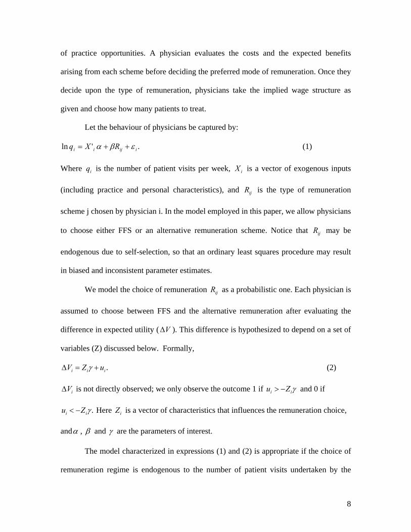
Let the behaviour of physicians be captured by:

.'ln iijii RXq εβα ++= (1)

Where iq is the number of patient visits per week, iX is a vector of exogenous inputs

(including practice and personal characteristics), and ijR is the type of remuneration

scheme j chosen by physician i. In the model employed in this paper, we allow physicians

to choose either FFS or an alternative remuneration scheme. Notice that ijR may be

endogenous due to self-selection, so that an ordinary least squares procedure may result

in biased and inconsistent parameter estimates.

We model the choice of remuneration ijR as a probabilistic one. Each physician is

assumed to choose between FFS and the alternative remuneration after evaluating the

difference in expected utility ( VΔ ). This difference is hypothesized to depend on a set of

variables (Z) discussed below. Formally,

.iii uZV +=Δ γ (2)

iVΔ is not directly observed; we only observe the outcome 1 if γii Zu −> and 0 if

.γii Zu −< Here iZ is a vector of characteristics that influences the remuneration choice,

andα , β and γ are the parameters of interest.

The model characterized in expressions (1) and (2) is appropriate if the choice of

remuneration regime is endogenous to the number of patient visits undertaken by the

9

physician. The econometrics literature suggests two methodological approaches to this

type of problem: an instrumental variable (IV) estimator, and a treatment effects (TE)

estimator (sometimes referred to as the restricted control function approach). The

estimation of the TE model involves a probit regression for equation (2) and an OLS

regression for equation (1) augmented by the hazard function from the probit model

(Heckman and Hotz, 1989; Greene, 2003; Wooldridge, 2002). In the IV approach,

residuals from a linear probability model on the indicator function (equation 2) are

included in the second stage in place of the hazard rate. The TE model assumes that

iiu ε and follow a bivariate normal distribution: it produces consistent and efficient

structural parameters, provided that the probit model is correctly specified. The IV

estimator, by contrast, is free from this distributional assumption, but the estimates are

consistent only if the instruments satisfy certain identification requirements, as discussed

below.6 Vella and Verbeek (1999) demonstrate that if the bivariate normality assumption

is satisfied and no other complications are present, the IV and TE estimators produce

similar results; they recommend comparing the estimated results from both models

(which we do).7

In the context of the TE model, the endogeneity of the remuneration scheme is

captured by the correlation between the residuals ε and u (rho) in equations (1) and (2).

If the estimate of rho is statistically significant, then there are, indeed, important

unobservable factors influencing the choice of remuneration scheme and thus neglecting

6 Note that the IV procedure is inefficient in the presence of heteroscedasticity. A rejection of the null hypothesis of homoscedasticity leads to two possible options. The first option is to use the robust Huber-White sandwich estimator of variance for the IV estimator. The second option is to use a two-step generalized method of moment (GMM) procedure, which is more efficient (Hayashi, 2000). Since we found an unknown form of heteroscedasticity in our data, the GMM estimation procedure is employed. 7 An extensive discussion on the estimation procedures and the statistical properties of the estimators can be found in Madala (1983) and Vella (1998)

10

selectivity issues would likely to give an inaccurate picture of the relative strengths of the

two remuneration regimes.8 In the IV procedure, the endogeneity of the remuneration

scheme can be detected using the Durbin-Wu-Hausman test statistic (Wooldridge, 2002;

Baum et al., 2003).

The TE model is extremely sensitive to the specification of the selection equation

and the structural equation. In order to render the model as robust as possible, it is

necessary to include several variables that affect the remuneration choice but not patient

visits per week; for identification purposes, at least one variable must have this property.

The IV method requires that all variables included in Z satisfy the requirements of

instruments relevance, over identifying restrictions and weak instruments.

Economic theory and the existing literature suggest a number of variables that

may affect the choice of remuneration but not the number of weekly patient visits. These

variables essentially reflect physicians’ preferences towards risk, tastes and the

characteristics of market demand and supply (Conrad et al., 2002; Gaynor and Pauly,

1990; Gaynor and Gertler, 1995). In this paper, four instruments are used to capture

differences in physicians’ preferences, tastes and risk perceptions. Some physicians may

have predisposition towards non-practice related activities, and thus are more likely to

choose a non-FFS scheme. If the physician has a propensity to undertake research, teach

or pursue other non-work related interests, then he or she would be more likely to choose

a salaried practice or other non-FFS modes of remuneration. Three dichotomous

variables, RESEARCH, TEACHING and NON-WORK-INTERESTS capture these

8 The TE model is estimated using the maximum likelihood method rather than the two-step method because it has the desirable properties of consistency and efficiency. We also use the robust Huber-White sandwich estimator of variance to correct for the unknown form of heteroscedasticity present in the data.

11

preferences. Note that these variables are based on responses regarding the factors that

motivated physicians at the beginning of their career, and hence they are exogenous to

the number of patient visits currently undertaken. From an economic perspective, these

tastes and preferences may reflect a lower valuation of direct patient care activities

associated with non-FFS modes of remuneration, or a low marginal utility of professional

income.

Finally, the way the physician prefers to be paid is another instrument governing

physician’s tastes and risk perceptions. Those who have a preference towards fee-for-

service may value leisure less than income and have a tendency to substitute leisure for

work. Although this preference for FFS can also be correlated with the number of office

visits, the maintained hypothesis in this paper is that it influences patient visits through

the manner in which it remunerates the physician. PREFER_FFS is thus a dummy

variable that takes on a value of 1 if the physician is preferred to be paid by FFS and zero

otherwise.9 We demonstrate in the empirical section that the exclusion of this variable

from the patient visit equation is valid.

4. Data and Variable Specifications

The data for this study are drawn mostly from the family physician component of

the 2004 National Physician Survey (NPS). The NPS furnishes a broad range of

information on the family physician’s allocation of time, the number of patient visits,

physician characteristics, practice patterns, type of patient population and method of

remuneration. This survey was sent to all licensed family physicians/general practitioners

9 Several instruments capturing the demand and supply factors were considered in earlier versions of this paper, but the overall results suggested that they contributed very little to explaining the choice of remuneration.

12

in Canada during early 2004 (February to June). Of the 30,903 eligible family

physicians/general practitioners, 11,041 replied to the survey leading to an overall

response rate of 36%. CIHI (2005) analyzed the respondents and non-respondents of this

survey and concluded that those who replied to the survey are representative of the

physician population at large with respect to specialty, age, gender and other

demographic characteristics.10 We deleted 543 records because the source of self-

reported income from all remuneration types did not add up to 100 percent. Direct patient

care hours are missing for about 2000 physicians, 255 physicians spent fewer than 10

hours per week on direct patient care, and some 600 physicians reported seeing fewer

than 10 patients per week. After deleting all missing observations and inappropriate

records, we were left with 7,352 observations suitable for our analysis.

The dependent variable in this study is the natural log of patient visits per week.

We restrict our attention to physicians who conducted at least ten patient visits per week

and who worked 10 to 80 hours per week in direct patient care to eliminate the influence

of outliers in the sample.

While it would be interesting to examine simultaneously the choices facing the

physician, we lack sufficient observations to pursue a selection bias correction based on

the multinomial logit model proposed in the recent literature (e.g., Bourguignon et al.,

2007). Moreover, econometrically, it is much easier to examine binary decisions which

also allows for a straightforward correction of any endogeneity bias in the data. The

paper focuses on four binary remuneration choices: FFS vs. Alternative; FFS vs. Mixed;

10 For detailed response patterns across provinces and analysis pertaining to respondents and non-respondents, see CIHI (2005). Aside from knowing that the respondents have similar demographic characteristics to the physician population, we do not know the extent to which the sample of physicians responding to the questionnaire is biased in some other way.

13

FFS vs. NFFS and FFS vs. Salary. The alternative, mixed, NFFS and salary

classifications are not mutually exclusive rather they are finer subsets of each other, with

the alternative scheme being the most inclusive category and salary being the least.11

The alternative remuneration scheme refers to the situation where family

physicians are paid other than by FFS. Of the 7,352 observations in our data, 4,239 are

categorized as FFS and the remaining 3,113 observations are thus classified as

alternative. These alternative arrangements comprise a mixture of different types of

payment: on average, 38% of income is received from FFS payments, 22.5% from salary,

3.3% from capitation, 23.3% from sessional/hourly payments, 8% from service contracts,

1.3% from incentives and premiums and 3.7% from others venues. A mixed

remuneration refers to the situation where physicians obtain 90% or more of their

professional income from a combination of payment schemes: no physician in this

classification receives 90% or more of his/her professional income from a single payment

scheme. This type of remuneration scheme resembles a blended payment system, except

that it is the physicians themselves who decide upon the blend and not the public

insurer.12 There are 2,187 respondents in our data set whose remuneration can be

classified as mixed, receiving, on average 53% of their income from FFS payments. A

NFFS scheme, by contrast, is defined as when physicians obtain 90% or more of their

professional income from a non-FFS scheme. 926 physicians in our sample are classified

as non-FFS: notice that this figure plus the mixed remuneration physicians comprise the 11 The estimated coefficients were found to be statistically different from each other in the second stage OLS regressions hence we present all four decisions. 12 Blended remuneration terminology refers to a situation where a provincial government signs a contract with physicians to pay in accordance with a predetermined blended formula. Mixed remuneration, on the other hand, refers to a situation where the physician decides on his/her own to practice in multiple remuneration settings. There are some exceptions in Ontario as a formal blended method of remuneration was introduced in 2002, and by 2004 some 400 physicians were working in blended remuneration, so our sample might include a few observations which may not be strictly categorized as mixed.

14

entire alternative payment scheme. Finally, salaried remuneration is when physicians

receive at least 90% of their professional income from salaried payments. 711 of the 926

NFFS physicians are classified as salaried.

Several variables suggested by the existing literature are used in the empirical

model, including physician gender, marital status, experience, and whether or not the

physician is an international medical graduate. Direct patient care hours by the reporting

physician is another important variable included in the visit equation, and it is often

regarded as an effort variable (Gaynor and Pauly, 1990).13 Following Reinhardt (1972),

we include both the natural logarithm of hours (lnH) and the number of hours worked, H,

consistent with a U-shaped average cost curve.

A wide variety of practice characteristics are included in the analysis. A dummy

variable captures if a physician shares patient care with another family physician in the

main patient care setting. A series of dummy variables denote whether or not a

physician’s practice has specialists, nurse practitioners, nurses and/or midwives. Patient-

mix is represented by seven dummy variables reflecting if the practice is comprised of

more than 10% of the following patient populations: individuals with chronic mental

illness or permanent physical disabilities, addicts, people living in poverty, aboriginals,

homeless people, transient or seasonal people, and recent immigrants. Provincial fixed

effects are captured by a series of provincial dummy variables with Ontario as the

reference category.

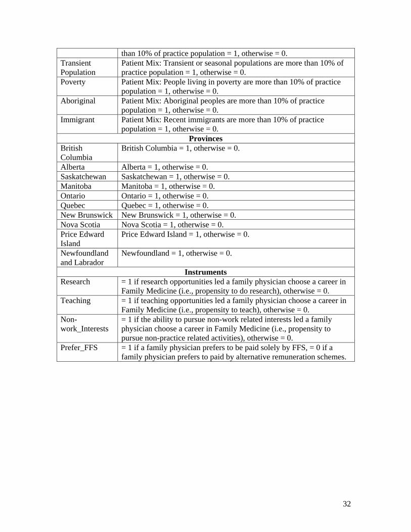
Table 1 describes the list of the dependent, explanatory and selection variables

used in this paper and table 2 presents the corresponding descriptive statistics. Clearly,

13 Direct patient care includes patient care in office/clinic, homecare, patient care in emergency room, hospital based activities and other inpatient care activities in institutions.

15

the average number of patient visits per week is much higher in a fee-for-service practice

than in the non-FFS and salary practices: 134 versus 78 and 72 respectively. Moreover,

FFS physicians are spending less time per patient than those paid by an alternative

method. Women are clearly more drawn to compensation schemes other than FFS when

compared to men; and, if we look at the recent cohort of medical-school graduates, most

of whom are female, we see that younger women graduates are more inclined to practice

in NFFS than in the FFS settings. Finally, FFS practices are different than other practices

in terms of the tendency of their physicians to not work directly with other health-care

specialists, as well as in terms of the characteristics of the patients treated. In other words,

a glance at table 2 reveals clear differences across the different remuneration models –

with the starkest contrast being between FFS and salaried practices.

INSERT Tables 1-2

5. Estimated Results

In an effort to verify the robustness of our results and to ensure that our results are

not an artifact of the sample chosen, we run three different econometric models with four

different samples. The main results discussed in the paper come from the IV GMM

procedure which we believe to be the best way to deal with the physician selection

problem, and are reported in table 3.14 (Notice that each procedure entails estimating four

regressions, one for each of the aforementioned binary choices facing the physician). We

also estimated the model using the TE and OLS procedures: the differences across the IV

14 The estimates from the TE models largely corroborate the main findings of the IV GMM. Moreover, the estimated correlation coefficients (rho’s) across the error terms of the participation decisions and the output decisions are positive and statistically significant, suggesting that these decisions are not independent of each other.

16

GMM and TE approaches are small, while the OLS results are clearly different. For the

sake of brevity, and in order to focus on the variables of interest to this study, table 4

simply reports the estimated coefficients on the remuneration scheme for these alternative

approaches, suppressing all other estimated parameters.

We need to examine whether the estimated impact on patient visits of each

remuneration scheme is robust. It may be that our analysis is unduly affected by the

inclusion of rural and remote practices because provincial governments often use

financial incentives to motivate physicians to work in these jurisdictions. Furthermore,

the choice of remuneration models facing physicians in rural areas is likely to be much

smaller than the choice facing urban practitioners. In order to control for these factors, we

restricted the sample to physicians who practiced in health regions where at least 50% of

the total population is urban according to the 2001 Census.15 The estimated coefficients

for the four different remuneration schemes (again, with FFS as the reference category in

each of the four regressions) with this restricted sample are presented in table 4. We

consider two possibilities in which physicians may be locked into a particular practice

pattern, experiencing significant psychic costs as well as other barriers to switching out of

that pattern. First, older physicians may have higher switching costs. Thus we excluded

physicians aged 60 and over in the sample. Second, FFS physicians who already practice

in a collaborative setting are likely to find it easier to switch to a remuneration scheme

which requires collaboration. We hence restricted the sample to those physicians who

share at least three of the following six items with other physicians: office space,

equipment, expenses, patient records, on-call and staff. Once again, the estimated

coefficients on the remuneration scheme for the four regressions are reported in table 4. 15 The full sample is comprised of 100 health regions while this restricted sample has 66.

17

5.1 Econometric Test Results

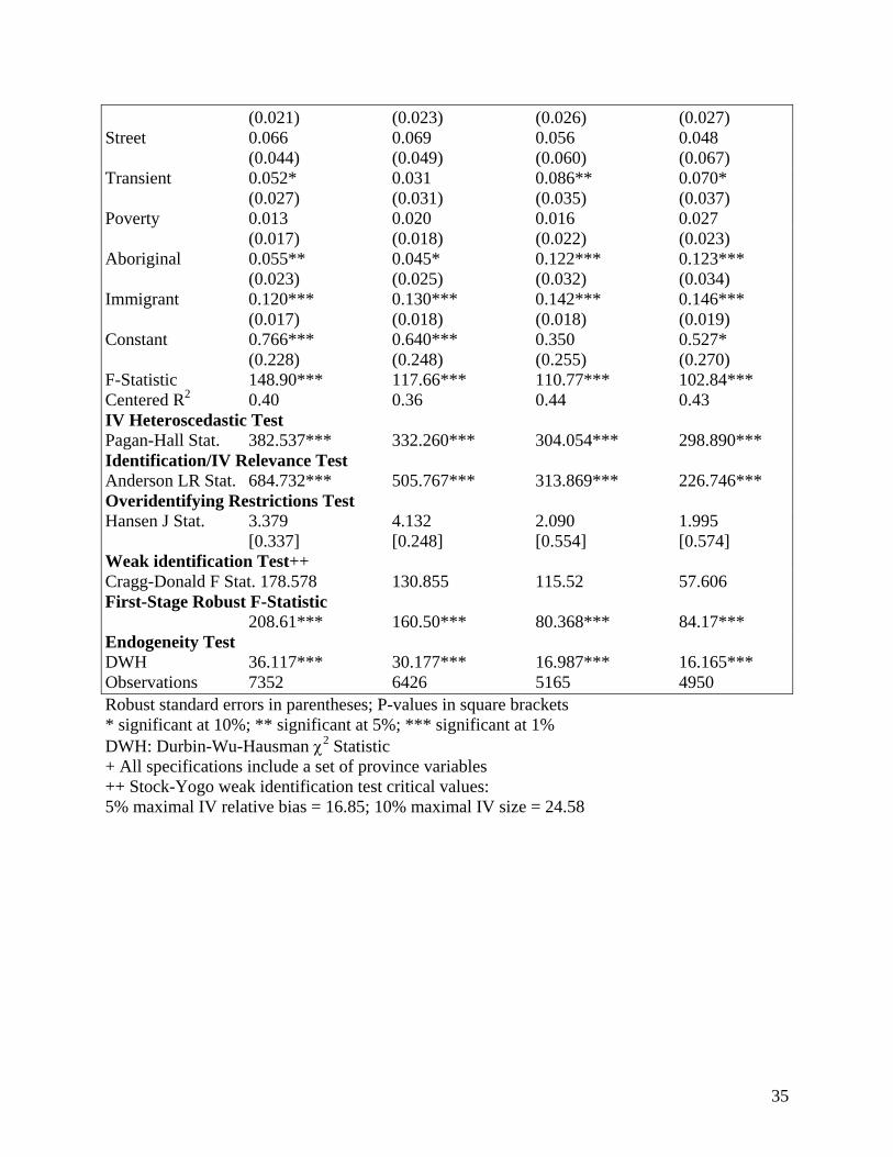
The test results regarding identification for the full sample are presented at the

bottom of table 3 and the results for the restricted samples are presented in table 5. The

estimated coefficients on the four instruments in the first stage of the IV procedure and

the associated test results on exogeneity and instrument redundancy are presented in table

6. In order for an instrument to be valid, it must be correlated with the included

endogenous regressor and orthogonal to the errors (Wooldridge, 2002). Since the

Anderson canonical correlations likelihood ratio test statistic is significant at the 1%

level, we conclude that the instruments are relevant and pass the under identification

requirement. But it is essential to ensure that the instruments also pass over-identification

restrictions. In the context of the IV GMM and the presence of heteroscedasticity, the

Hansen J-statistic test is the relevant test procedure (Baum et al., 2003). A rejection of the

null hypothesis that the instruments are uncorrelated with the error term and they are

correctly excluded from the structural equation raises questions about the validity of

instruments. The Hansen J-statistic is insignificant for all of the estimated models

considered, confirming that our instruments are valid. Since we also hypothesize that

each instrument has certain strength, the C-statistic test is used to test the validity of

subsets of instruments: that is, excluding one instrument from the full set of instruments

and comparing the Hansen J-statistics for the restricted and unrestricted models

(Eichenbaum et al., 1988; Hayashi, 2000; Baum et al., 2003). The C-statistics also

presented in table 5 suggest that all instruments satisfy orthogonality conditions with at

least 5% level of significance. We also conduct likelihood ratio based tests to see if an

18

excluded instrument is redundant in the sense that the asymptotic efficiency of the

estimation is unaffected by using it (Hall and Peixe, 2000). In most instances, the null

hypothesis that the instrument is redundant is rejected at the 1% significance level,

although some instruments are not significant in some models, as presented in table 6.16

It is also necessary to test whether the IV estimates suffer from weak instrument

problems; if the instruments are weak then the IV estimator continues to be biased in the

same direction as ordinary least squares estimator, the distribution of the estimator is non-

normal and the conventional asymptotics fail (Bound et al., 1995). Stock and Yogo

(2005) developed a weak-identification F-statistic procedure to examine the bias

associated with IV estimator. These weak identification test results are presented in table

3 for the IV GMM model. For all models considered in this paper, the bias and size

distortion is small, thus we reject the null hypothesis that the IV estimator is weakly

identified.

The test of whether or not the OLS procedure yields inconsistent estimates is the

Durbin-Wu-Hausman test of the endogeneity of regressors. An examination of the

Durbin-Wu-Hausman Chi-squared test statistic reveals that the null hypothesis that the

remuneration scheme is exogenous is rejected at the 1% level of significance in all

specifications.

5.2 Does Selection Matter?

We begin with the important question of whether controlling for selection bias

matters when it comes to estimating the impact of the remuneration scheme on patient

visits per week. Does correcting for selectivity have an economically important effect? 16 The entire first-stage regression results are available from the corresponding author upon request.

19

To address this question, it is useful to look at the expected value of patient visits if the

physician chose an alternative remuneration scheme (the treatment) versus if he chose

FFS (no treatment). From Greene (2003, 788) we can express the difference in the

expected value of the treatment and non-treatment group as:

( )[ | 1, , ] [ | 0, , ] *( ); 1i i i i i i i i i i iE q R X Z E q R X Z rho A A εβ σ φ⎡ ⎤= − = = + = Φ −Φ⎣ ⎦ (3)

The right-hand-side of expression is the total effect on patient visits per week associated

with choosing the alternative regime over the FFS one, ceteris paribus. We can

decompose this total effect into two parts: the first part, β, may be called the pure

incentive effect arising from the remuneration scheme, while the second part, rho*A is the

selection effect.17 Notice that estimating expression (1) using the OLS procedure is

tantamount to forcing the selection effect to be zero, in which case the entire effect will

be being picked up by the estimated coefficient on the remuneration scheme, namely β.

The empirical results presented in table 4 can be used to estimate the incentive

and selection effects. The estimated coefficients on alternative, mixed, NFFS and salary

remuneration from the OLS procedure are -0.23, -0.18, -0.40 and -0.45, respectively. The

corresponding estimated coefficients from the IV GMM procedure are -0.47, -0.43, -0.73

and -0.86. All of these estimates indicate that family physicians paid other than by FFS

see fewer patients per week compared to those paid by fee-for-service. A glance at table 4

reveals just how robust these estimated effects are. Irrespective of the econometric

17 We have used natural logs of patient visits instead of levels due to skewed nature of the data. As a result, the estimated expected number of patient visits is more complex to compute. One cannot simply reverse this transformation (taking the antilog of the predicted log of patient visits) as this will cause a retransformation bias. One needs to use appropriate smearing estimator to correct for this bias (Duan, 1983; Manning and Mullahy, 2001). Given the complex issues involved in employing suitable smearing estimators for non-linear models, we resorted to the Halvorsen-Palmquist adjustment as an alternative approach (Halvorsen and Palmquist, 1980). We use the percentage interpretation of a dummy variable in the context of a semi-logarithmic model with and without selection effect and decompose the overall remuneration effect into incentive and selection effects.

20

procedure employed and the sample under investigation, salaried physicians always have

fewer patient visits per week relative to all other schemes, and FFS physicians always

have the most.

However, the OLS procedure consistently understates the impact of remuneration

on the number of patient visits. The OLS procedure indicates that the effect of the

alternative remuneration is to reduce the number of patient visits by 20%, while the IV

GMM estimates suggest that the drop is 37%. A similar discrepancy is found when

comparing the impact of choosing a mixed regime using the OLS model versus the IV

GMM approach: 16% compared to 35%. The OLS results indicate that NFFS

remuneration reduces the number of patient visits by 33% in comparison to FFS

remuneration, while the estimate from the IV GMM procedure is a 52% reduction.

Finally, OLS finds a drop in patient visits of 36% when comparing salary to FFS

physicians, as opposed to a 58% difference when correcting for selectivity.

In effect, the OLS results can be interpreted as comprising both the incentive

effect arising from the different remuneration schemes plus any effect stemming from the

fact that physicians are self-selecting into the different schemes. By contrast, the IV

GMM approach corrects for the selection effect and hence the estimated coefficient on

the remuneration scheme variable captures the pure incentive effect. Thus, we can look at

the difference across these two estimated effects to obtain an approximation of the

magnitude of the self-selection effect. For instance, going from a fee-for-service

environment to a salaried one would result in a total fall of 36% of patient visits per week

(from the OLS results) which is comprised of a 58% reduction arising from the negative

incentive effects plus a 22% increase in the number of visits per week stemming from the

21

positive selection effect. Two points should be noted. First, across the board, irrespective

of which remuneration scheme is being compared to FFS, of what procedure is used to

correct for the physician selection bias, and of the data sample employed, the selection

effect is positive. The unobservable characteristics leading individuals to choose schemes

other than FFS would cause them to see more patients per week. The magnitude of

selection effect is in the range of 17% to 27% across the four remuneration schemes in

four samples examined. The second point is that while the selection effect would lead

physicians to conduct more patient visits per week, the incentive effect arising from the

remuneration scheme is large and negative, overwhelming the positive selection effect.

One important implication of our findings is that the alternative remuneration

schemes are not attracting physicians who are innately “less productive” – on the

contrary, they appear to be attracting physicians with desirable characteristics. However,

it is the incentive effects stemming from the schemes themselves that are causing

difficulties. Assuming that a policy objective is for physicians see a larger number of

patients per week, it would seem worthwhile to explore the features of the alternative

remuneration models which appear to be working against this objective.

We can get a sense of what factors are affecting the selection effect by examining

the instruments chosen to capture the remuneration decision. From table 6 we see that all

of the instruments exert a statistically significant influence on the decision to choose the

alternative, mixed, NFFS or salary scheme with the exception of research; furthermore,

the signs of their influence are the same across the four estimations. The two variables

indicating a propensity to undertake non-practice related activities, have positive

estimated coefficients: physicians who had a desire to teach or had strong non-work-

22

related interests, are more likely to choose a remuneration scheme other than FFS. As

expected, a stated preference to be paid by FFS is negatively associated with the choice

of non-FFS remuneration schemes.

5.3 Other Factors Influencing Visits per Week

In addition to remuneration schemes, several other factors influence the number

of patient visits per week. For instance, the number of hours worked by a physician

clearly matters. We see that the estimated coefficient on the natural logarithm of hours

worked is positive, while that on the number of hours worked in levels is negative. Taken

together, these estimates mean that the number of visits per week increases with hours

worked at a decreasing rate, reflecting diminishing marginal productivity of hours – as

expected.

The gender of the physician also matters: females tend to have fewer patient visits

per week, consistent with results found elsewhere. Being married is associated with a

higher number of visits per week, again according with expectations. It does not seem to

matter if the physician obtained his or her medical degree at a foreign institution,

however a concave relationship between age and patient visits is found. The turning point

for age is in the neighborhood of 45 years, which implies that after this point physicians

would tend to see fewer patient visits.

Whether or not the practice is part of a group, be it a group with other family

physicians or with other specialists, matters. Family physicians practicing with other

family physicians tend to have more patient visits per week, while those who practice

with specialists tend to have fewer visits per week. This first result seems quite sensible,

23

while the second requires more thought. One possibility is that physicians who practice

with specialists are more apt to refer their patients to the specialist and hence have fewer

follow-up visits. There is no discernable impact on patient visits from the presence of

midwives.

Several patient characteristics were included as explanatory variables in order to

help capture any selection bias that may arise from patient selection. Unfortunately, the

data set is not ideal in this regard: it provides information on whether the practice has

10% or more of patients with certain characteristics. The 10% threshold may be too small

to capture adequately the impact of having a preponderance of certain kinds of patients in

the practice. Nevertheless, we have to work with what we have. Two characteristics stand

out as having a negative impact on the number of patients seen, across the board:

practices with at least 10% of patients with mental conditions tend to see fewer patients

per week, as do those with at least 10% of patients with addictions. Arguably, when such

patients visit their physicians, they require longer-than-average consultations, hence

fewer visits are possible in any given work week. It is interesting to note that the presence

of people with physical disabilities does not have any perceptible impact on patient visits:

these people do not require any more time than patients without physical disabilities. The

same result holds for street people and poor people. In other words, it is not being poor or

homeless that matters, it is having mental conditions and addictions that command more

physician time. Having a transient population tends to increase the number of visits per

week, which may reflect the fact that the population is transient and hence not likely to

see a physician on a regular basis. The presence of 10% or more Aboriginal people in the

practice is also associated with more visits per week. Finally, we note that a practice with

24

10% or more immigrants also has a positive influence on the number of patients seen per

week. This result may be reflecting the ‘healthy-immigrant’ effect whereby immigrants

who are admitted to Canada may be healthier than the native born.

6. Conclusions and Policy Implications

The main goal of this paper was to examine the extent to which the incentives

embedded in remuneration schemes affect physician output. We were particularly

interested in ensuring that any effects arising from the fact that physicians self-select into

any given remuneration schemes were dealt with so that we could determine how

physicians react to the schemes, per se. For data reasons, and following others in the

literature, we use patient visits per week as our measure of output. Our results corroborate

the finding in the theoretical literature that remuneration schemes generate substantial

incentive effects (e.g., McGuire, 2000). We are able to take this finding even further and

decompose the overall effect into two parts: the pure incentive effect arising from the

remuneration scheme per se, and the selection effect arising from the fact that physicians

who choose alternative remuneration schemes differ systematically relative to those who

choose FFS scheme.

We find a positive selection effect at work. The physicians who choose alternative

remuneration would appear to have characteristics that would result in them seeing more

patients per week, ceteris paribus, relative to FFS physicians. In other words, if we were

able to run an experiment in which physicians could self-select into the remuneration

scheme of their choice, and then, unexpectedly, we constrained all of the schemes to be

25

the same, we would find that those who choose a non-FFS environment engaged in more

patient visits per week than those who choose the FFS scheme.

We also found a large negative incentive effect emanating from the remuneration

schemes once the selection effect is controlled for. FFS schemes appear to strongly

encourage physicians to see many more patients relative to alternative remuneration

schemes. From a measurement perspective, therefore, using a simple OLS procedure can

seriously underestimate the incentives arising from payment schemes.

An important public policy question is whether the incentives emanating from

alternative remuneration schemes are socially desirable, and, if not, how they can be

mitigated. Our results show that the physicians who choose alternative schemes are

clearly capable of seeing more patients. Of course, part of the problem may be that

physicians in salaried and other practices may have more complex patients who cannot be

turned out with the same speed as those in FFS practices. We have tried to control for

patient mix by controlling for patients with certain conditions, but certainly this could be

improved upon. However, it seems unlikely that patient mix alone explains this incentive

effect. Perhaps policy makers will have to mandate that salaried family physicians

undertake a certain number of patient visits per week in order to have a family practice –

akin to the requirement that university professors teach a certain number of hours per

week as part of their appointment.18

18 Universities are becoming increasingly sensitive to the fact that some professors – typically those with high research output – do not teach students. Thus, when one looks at one measure of output, the student-professor ratio, some departments look very good, yet when the actual average class size is measured, these departments fail abysmally.

26

Although physicians remunerated under FFS regime conduct a higher number of

patient visits per week when compared to those paid under alternative schemes, other

considerations are also be important. As our population is aging, and the numbers of

patients with complicated and chronic conditions increase, it may be desirable to

remunerate physicians such that they are encouraged to spend the required amount of

time with their patients rather than being penalized as is effectively the case under the

current FFS regime if a patient takes up too much time. Indeed, one weakness with this

current study is that it focuses solely on family practitioners. A more complete study,

would examine the impact on referral to specialists of having the front-line physicians

paid by FFS versus alternative schemes. One possibility is that spending more time in a

generalist’s office may reduce the amount of time necessary with a specialist – which

may make a lot of sense from the point of view of the public purse.

Our study does not discuss the welfare implications of the impact of moving from

FFS toward alternative forms of remuneration regimes. This would be a fruitful avenue

for additional research. It would be interesting to conduct additional analysis to tease out

the impact of remuneration regimes on physician incomes, costs to the health care system

and patient health improvements and ascertain policy implications for social welfare by

designing appropriate regulatory structure on physician’s behaviour.

References

Armour, B. S., Pitts, M. M., Maclean, C., Cangialose, M., Kishel, M., Imai, H., and Etchason, J. 2001. The effect of explicit financial incentives on physician behaviour. Archives of Internal Medicine 161(10), 1261-1266.

27

Barro, J. R., and Beaulieu, N. R. 2003. Selection and improvement: physician response to financial incentives. NBER Working Paper # 10017. National Bureau of Economic Research, Cambridge, MA.

Baum, C.F., Schaffer, M.E., and Stillman, S. 2003. Instrumental variables and GMM: Estimation and testing. Stata Journal 3, 1-31.

Bound, J, Jaeger, D.A., and Baker, R.M. 1995. Problems with instrumental variables estimation when the correlation between the instruments and the explanatory variables is weak. Journal of the American Statistical Association 90, 443-450.

Bourguignon, F., Fournier, M., and Gurgand, M. 2007. Selection bias corrections based on the multinomial logit model: Monte Carlo comparisons. Journal of Economic Surveys 21(1), 174-205.

Canadian Institute for Health Information. 2008. Physicians in Canada: The Status of Alternative Payment Programs, 2005-2006. Canadian Institute for Health Information, Ottawa.

Canadian Institute for Health Information. 2007a. The status of alternative payment programs for physicians in Canada, 2004-2005 and preliminary information for 2005-2006. Canadian Institute for Health Information, Ottawa.

Canadian Institute for Health Information. 2007b. Distribution and Internal Migration of Canada’s Physician Workforce, Canadian Institute for Health Information, Ottawa.

Canadian Institute for Health Information. 2005. 2004 National Physician Survey response rates and comparability of physician demographic distributions with those of the physician population, Canadian Institute for Health Information, Ottawa.

Carlsen, F. and Grytten, J. 2000. Consumer satisfaction and supplier induced demand. Journal of Health Economics 9, 731-753.

Carlsen F., Grytten, J., and Skau, I. 2003. Financial incentives and the supply of laboratory tests. European Journal of Health Economics 4, 279-285.

Chaix-Couturier, C., Durand-Zalesky, I., Jolly, D., and Durieux, P. 2000. Effects of financial incentives on medical practice: results from a systematic review of the literature and methodological issues. International Journal for Quality in Health Care 12(2), 133-142.

Conrad, D. A., Sales, A., Liang, S., Chaudhuri, A., Maynard, C., Pieper, L., Weinstein, L., Gans, D., and Piland, N. 2002. The impact of financial incentives on physician productivity in medical groups. Health Services Research 37(4), 885-906.

Conrad, D. A., and Christianson, J. B. 2004. Penetrating the ‘black box’: financial incentives for enhancing the quality of physician services. Medical Care Research and Review 61(3), 37S-68S.

Conrad, D. A., Maynard, C., Cheadle, A., Ramsey, S., Marcus-Smith, M., Kirz, H., Madden, C.A., Martin, D., Perrin, E. B., Wickizer, T., Zierler, B., Ross, A., Noren, J., Liang, S.Y. 1988. Primary care physician compensation method in medical groups: does it influence the use and cost of health services for enrollees in managed care organizations? Journal of American Medical Association 279(11), 853-858.

Duan, N. 1983. Smearing estimate: a nonparametric retransformation method. Journal of the American Statistical Association 78(383), 605-610.

28

Eichenbaum, M.S., Hansen, L.P., and Singleton, K.J. 1988. A time series analysis of representative agent models of consumption and leisure. Quarterly Journal of Economics 103, 51–78.

Gaynor, M., and Pauly, M. V. 1990. Compensation and productive efficiency in partnerships: Evidence from medical group practice. Journal of Political Economy 98(3), 544-573.

Gaynor, M., and Gertler, P. 1995. Moral hazard and risk spreading in partnerships. Rand Journal of Economics 26(4), 591-613.

Gosden, T., Forland, F., Kristiansen, I. S., Sutton, M., Leese, B., Giuffrida, A., Sergison, M., and Pederson, L. 2004. Capitation, salary, fee-for-service and mixed systems of payment: effects on the behaviour of primary care physicians [Cochrane review]. In: The Cochrane Library, Issue 2. Chichester, UK: John Wiley & Sons, Ltd.

Gosden, T., Forland, F., Kristiansen, I. S., Sutton, M., Leese, B., Giuffrida, A., Sergison, M., and Pederson, L. 2001. Impact of payment method on behaviour of primary care physicians. Journal of Health Services Research and Policy 6(1), 44-55.

Greene, W. H. 2003. Econometric Analysis, 5th edition, Prentice Hall, New Jersey. Grytten, J., and Sørensen, R. J. 2001. Type of contract and supplier-induced demand for

primary physicians in Norway. Journal of Health Economics 20, 379-393. Hadley, J., and Reschovsky, J. D. 2006. Medicare fees and physician’s medicare service

volume: beneficiaries treated and services per beneficiary. International Journal of Health Care Finance and Economics 6(2), 131-150.

Hall, A.R., and Peixe, F.P.M. 2000. A consistent method for the selection of relevant instruments. Econometric Society World Congress 2000, Contributed Papers, Number 0790. http://ideas.repec.org/p/ecm/wc2000/0790.html

Halvorsen, R, and Palmquist, R. 1980. The interpretation of dummy variables in semilogarihmic equations. American Economic Review 70, 474-475.

Hayashi, F. 2000. Econometrics (1st edn). Princeton University Press, New Jersey. Heckman, J.J., and Hotz, V.J. 1989. Choosing among alternative non-experimental

methods for estimating the impact of social programs: the case of manpower training. Journal of the American Statistical Association 84, 862-874.

Hemenway, D., Killen, A., Cashman, S. B., Parks, C. L., and Bicknell, W.J. 1990. Physicians’ response to financial incentives. The New England Journal of Medicine 322,1059-1063.

Hickson, B., Altemeier, A., and Perrin, M. 1987. Physician reimbursement by salary or fee-for-service: Effect on physician practice behavior in a randomized prospective study. Pediatrics 80(3), 344-350.

Holahan, J., Dor, A., and Zuckerman, S. 1990. Understanding the recent growth in Medicare physician expenditures. Journal of American Medical Association 263(12), 1658-1661.

Hurley, J., Labelle, R., and Rice, T. 1990. The relationship between physician fees and the utilization of medical services in Ontario. Advanced Health Economics and Health Services Research 11, 49-78.

Hurley, J., and Labelle, R., and Rice, T. 1990. Relative fees and the utilization of physicians’ services in Canada. Health Economics 4(6), 419-438.

29

Hutchinson, J. M., and Foley, R. N. 1999. Method of physician remuneration and rates of antibiotic prescription. Canadian Medical Association Journal 160, 1013-1017.

Keeler, E. B. 1996. Equalizing physician fees had little effect on cesarean rates. Medical Care Research Review 53(4), 465-471.

Kristiansen, I. S., and Mooney, G. 1993. The general practitioner’s use of time: Is it influenced by the remuneration system? Social Science & Medicine 37, 393-399.

Kristiansen I., and Holtedahl, K. 1993. The effect of the remuneration system on the general practitioner’s choice between surgery consultations and home visits. Journalof Epidemiology and Community Health 47, 481–484.

Luft, H. S. and Miller, R. H. 1988. Patient selection in a competitive health care system. Health Affairs 7(3), 97-119.

Madala, G.S. 1983. Limited-Dependent and Qualitative Variables in Econometrics. Cambridge: Cambridge University Press.

Manning, W.G., and Mullahy, J. 2001. Estimating log models: to transform or not to transform. Journal of Health Economics 20(4), 461-494.

Manning, W.G., Newhouse, J.P., Duan, N., Keeler, E.B., Leibowitz, A., and Marquis, M.S. 1987. Health insurance and the demand for medical care: Evidence from a randomized experiment. American Economic Review 77, 251-277.

Maynard, A., Marinker, M., and Pereira Gray, D. 1996. The doctor, the patient and their contract III. Alternative contracts: are they viable? British Medical Journal 292, 1438-1440.

McGuire, T. 2000. Physician agency, in The Handbook of Health Economics, ed. A. Cuyler and J. Newhouse. Amsterdam: Elsevier Science.

Reinhardt, U. 1972. A production function for physician services. Review of Economics and Statistics 54, 55-66.

Reschovsky, J. D., Hadley, J., and Landon, B. E. 2006. Effects of compensation methods and physician group structure on physician’s perceived incentives to alter services to patients. Health Services Research 41(4), 1200-1220.

Scott, A. 2000. Economics of general practice, in The Handbook of Health Economics, ed. A. Cuyler and J. Newhouse. Amsterdam: Elsevier Science.

Scott, A., and Hall, J. 1995. Evaluating the effect of GP remuneration: problems and prospects. Health Policy 31, 183-195.

Sørensen, R. J., and Grytten, J. 2003. Service production and contract choice in primary physician services. Health Policy 66, 73-93.

Stock, J.H., and Yogo, M. 2005. Testing for weak instruments in linear IV regression, in DWK Andrews and JH Stock (eds.) Identification and Inference for Econometric Models: Essays in Honor of Thomas Rothenberg. Cambridge: Cambridge University Press, 80–108.

Town, R., Kane, R., Johnson, P., and Butler, M. 2005. Economic incentives and physicians’ delivery of preventive care: A systematic review. American Journal of Preventive Medicine 28(2), 234 – 240.

Vella, F. 1998. Estimating models with sample selection bias: a survey. Journal of Human Resources 33(1), 127-169.

Vella, F., and Verbeek, M. 1999. Estimating and interpreting models with endogeneous treatment effects. Journal of Business and Economic Statistics 17(6), 473–478.

30

Wilensky, G. R and Rossiter, L. F. 1986. Patient self-selection in HMOs. Health Affairs 5(1), 66-80.

Wooldridge, J.M. 2002. Econometric analysis of cross section and panel data. The MIT Press, Massachusetts.

Zweifel, P., and Breyer, F. 1997. Health Economics. Oxford University Press: Oxford.

31

Table 1 Variable Definitions

Variable Definition Dependent Variables

LnQ Natural log of office patient visits/week for reporting physician (>=10 visits).

Remuneration Schemes FFS = 1 if a family physician earns 90%+ of professional income from the

fee-for-service remuneration scheme, otherwise = 0. Alternative = 1 if a family physician does not earn 90%+ of professional income

from the FFS remuneration scheme, = 0 if FFS. Mixed = 1 if a family physician earns 90%+ of professional income from a

combination of a pure remuneration schemes only, = 0 if FFS. NFFS = 1 if a family physician earns 90%+ of professional income from a

non-fee-for-service remuneration scheme, = 0 if FFS. Salary = 1 if a family physician receives at least 90%+ of professional income

from salary or sessional remuneration schemes, = 0 if FFS. Hours Worked

H Weekly input of reporting physician time in hours (>= 10 hours and <= 80 hours) providing direct patient care.

LnH Natural log of H. Physician Characteristics

Female Female = 1, male = 0. Married Married/ living with partner = 1, otherwise = 0. IMG International medical graduate = 1, Canadian medical graduate = 0. Age Age in completed years. Age Squared Square of Age.

Practice Characteristics FP = 1 if a family physician shares patient care with another family

physician in the main patient care setting, otherwise =0. Specialist = 1 if a family physician shares patient care with a specialist in the

main patient care setting, otherwise = 0. Nurse Practitioner

= 1 if a family physician shares patient care with a Nurse Practitioner in the main patient care setting, otherwise = 0.

Nurse = 1 if a family physician shares patient care with a Nurse in the main patient care setting, otherwise = 0.

Midwife = 1 if a family physician shares patient care with a Midwife in the main patient care setting, otherwise = 0.

Mental Patient Mix: Patients with chronic mental illness are more than 10% of practice population = 1, otherwise = 0.

Addiction Patient Mix: Patients with addictions more than 10% of practice population = 1, otherwise = 0.

Disability Patient Mix: Patients with permanent physical disabilities are more than 10% of practice population = 1, otherwise = 0.

Street Patient Mix: Homeless or street people/ transient populations are more

32

than 10% of practice population = 1, otherwise = 0. Transient Population

Patient Mix: Transient or seasonal populations are more than 10% of practice population = 1, otherwise = 0.

Poverty Patient Mix: People living in poverty are more than 10% of practice population = 1, otherwise = 0.

Aboriginal Patient Mix: Aboriginal peoples are more than 10% of practice population = 1, otherwise = 0.

Immigrant Patient Mix: Recent immigrants are more than 10% of practice population = 1, otherwise = 0.

Provinces British Columbia

British Columbia = 1, otherwise = 0.

Alberta Alberta = 1, otherwise = 0. Saskatchewan Saskatchewan = 1, otherwise = 0. Manitoba Manitoba = 1, otherwise = 0. Ontario Ontario = 1, otherwise = 0. Quebec Quebec = 1, otherwise = 0. New Brunswick New Brunswick = 1, otherwise = 0. Nova Scotia Nova Scotia = 1, otherwise = 0. Price Edward Island

Price Edward Island = 1, otherwise = 0.

Newfoundland and Labrador

Newfoundland = 1, otherwise = 0.

Instruments Research = 1 if research opportunities led a family physician choose a career in

Family Medicine (i.e., propensity to do research), otherwise = 0. Teaching = 1 if teaching opportunities led a family physician choose a career in

Family Medicine (i.e., propensity to teach), otherwise = 0. Non-work_Interests

= 1 if the ability to pursue non-work related interests led a family physician choose a career in Family Medicine (i.e., propensity to pursue non-practice related activities), otherwise = 0.

Prefer_FFS = 1 if a family physician prefers to be paid solely by FFS, = 0 if a family physician prefers to paid by alternative remuneration schemes.

33

Table 2: Descriptive Statistics FFS

(N = 4,239) Alternative (N = 3,113)

Mixed (N = 2,187)

NFFS (N = 926)

Salary (N = 711)

Variable Mean Std. Dev. Mean Std. Dev. Mean Std. Dev. Mean Std. Dev. Mean Std. Dev. Q H Female Married IMG Age FP Specialist Nurse Practitioner Nurse Midwife Mental Addiction Disability Street Transient Poverty Aboriginal Immigrant British Columbia Alberta Saskatchewan Manitoba Ontario Quebec New Brunswick Nova Scotia Newfoundland Price Edward Island Research Teaching Non-work_Interests Prefer_FFS

134.244 37.031 0.403 0.870 0.208 48.383 0.791 0.312 0.057 0.325 0.010 0.150 0.054 0.084 0.014 0.032 0.133 0.055 0.132 0.159 0.134 0.030 0.027 0.434 0.150 0.023 0.030 0.011 0.002 0.032 0.094 0.182 0.402

60.257 11.148 0.334 0.337 0.406 10.693 0.406 0.463 0.232 0.468 0.100 0.357 0.225 0.277 0.118 0.175 0.339 0.229 0.338 0.366 0.340 0.172 0.163 0.496 0.357 0.149 0.171 0.106 0.041 0.176 0.292 0.386 0.490

96.980 33.546 0.408 0.853 0.147 45.132 0.844 0.449 0.226 0.606 0.018 0.225 0.115 0.142 0.050 0.060 0.232 0.137 0.091 0.126 0.070 0.028 0.045 0.357 0.262 0.035 0.040 0.028 0.009 0.068 0.211 0.270 0.081

55.768 11.582 0.492 0.354 0.355 9.847 0.363 0.497 0.418 0.489 0.133 0.418 0.319 0.349 0.218 0.238 0.422 0.344 0.287 0.331 0.256 0.164 0.207 0.479 0.440 0.185 0.196 0.165 0.096 0.252 0.408 0.444 0.272

105.030 34.640 0.374 0.869 0.132 45.077 0.851 0.407 0.171 0.530 0.012 0.198 0.101 0.123 0.043 0.053 0.209 0.122 0.083 0.134 0.081 0.016 0.038 0.378 0.254 0.037 0.032 0.022 0.008 0.072 0.203 0.257 0.101

56.394 11.788 0.484 0.338 0.339 9.817 0.356 0.491 0.377 0.499 0.108 0.399 0.301 0.329 0.204 0.223 0.407 0.327 0.276 0.341 0.273 0.126 0.191 0.485 0.435 0.189 0.177 0.147 0.090 0.258 0.403 0.437 0.301

77.969 30.962 0.487 0.816 0.184 45.260 0.825 0.548 0.355 0.785 0.032 0.288 0.148 0.187 0.066 0.078 0.285 0.173 0.109 0.106 0.045 0.055 0.060 0.309 0.282 0.031 0.057 0.042 0.012 0.059 0.230 0.302 0.033

49.320 10.648 0.500 0.387 0.387 9.921 0.380 0.498 0.479 0.411 0.177 0.453 0.355 0.390 0.248 0.268 0.452 0.378 0.312 0.308 0.208 0.228 0.238 0.462 0.450 0.174 0.232 0.201 0.108 0.236 0.421 0.460 0.180

72.105 30.182 0.537 0.810 0.173 44.878 0.844 0.543 0.383 0.803 0.028 0.300 0.132 0.197 0.063 0.072 0.302 0.155 0.107 0.079 0.039 0.049 0.055 0.267 0.346 0.034 0.060 0.055 0.015 0.059 0.224 0.308 0.037

47.153 10.625 0.499 0.392 0.379 9.783 0.363 0.499 0.486 0.398 0.165 0.458 0.339 0.398 0.244 0.258 0.460 0.362 0.309 0.270 0.195 0.216 0.228 0.443 0.476 0.181 0.239 0.228 0.124 0.236 0.417 0.462 0.188

34

Table 3 Family Physician's Patient Visits per Week: IV GMM Estimation+

(Full Sample) (1) (2) (3) (4) Alternative Mixed NFFS Salary Remuneration Scheme Fee-for-service is the reference category Alternative -0.470*** (0.044) Mixed -0.434*** (0.049) NFFS -0.731*** (0.086) Salary -0.861*** (0.111) Hours Worked per Week on Direct Patient Care lnH 1.112*** 1.111*** 1.244*** 1.160*** (0.078) (0.086) (0.089) (0.095) H -0.013*** -0.013*** -0.018*** -0.016*** (0.002) (0.002) (0.003) (0.003) Physician Characteristics Female -0.178*** -0.174*** -0.158*** -0.150*** (0.013) (0.014) (0.014) (0.015) Married 0.030* 0.033* 0.019 0.013 (0.017) (0.019) (0.020) (0.021) IMG -0.018 -0.020 0.021 0.032 (0.017) (0.018) (0.020) (0.020) Age 0.031*** 0.035*** 0.033*** 0.034*** (0.004) (0.005) (0.005) (0.005) Age Squared -0.00035*** -0.00038*** -0.00036*** -0.00037*** (0.00005) (0.00005) (0.00006) (0.00006) FP 0.173*** 0.175*** 0.145*** 0.150*** (0.017) (0.018) (0.021) (0.021) Specialist -0.083*** -0.087*** -0.089*** -0.089*** (0.013) (0.014) (0.016) (0.016) NP -0.013 -0.001 0.091** 0.100** (0.020) (0.023) (0.036) (0.041) Nurse -0.015 -0.014 0.049** 0.057** (0.014) (0.014) (0.021) (0.023) Midwife -0.061 -0.100 -0.055 -0.062 (0.067) (0.080) (0.081) (0.090) Mental -0.078*** -0.090*** -0.077*** -0.072*** (0.018) (0.019) (0.022) (0.023) Addiction -0.120*** -0.117*** -0.152*** -0.160*** (0.030) (0.033) (0.039) (0.042) Disability -0.004 0.022 0.016 0.032

35

(0.021) (0.023) (0.026) (0.027) Street 0.066 0.069 0.056 0.048 (0.044) (0.049) (0.060) (0.067) Transient 0.052* 0.031 0.086** 0.070* (0.027) (0.031) (0.035) (0.037) Poverty 0.013 0.020 0.016 0.027 (0.017) (0.018) (0.022) (0.023) Aboriginal 0.055** 0.045* 0.122*** 0.123*** (0.023) (0.025) (0.032) (0.034) Immigrant 0.120*** 0.130*** 0.142*** 0.146*** (0.017) (0.018) (0.018) (0.019) Constant 0.766*** 0.640*** 0.350 0.527* (0.228) (0.248) (0.255) (0.270) F-Statistic 148.90*** 117.66*** 110.77*** 102.84*** Centered R2 0.40 0.36 0.44 0.43 IV Heteroscedastic Test Pagan-Hall Stat. 382.537*** 332.260*** 304.054*** 298.890*** Identification/IV Relevance Test Anderson LR Stat. 684.732*** 505.767*** 313.869*** 226.746*** Overidentifying Restrictions Test Hansen J Stat. 3.379 4.132 2.090 1.995 [0.337] [0.248] [0.554] [0.574] Weak identification Test++ Cragg-Donald F Stat. 178.578 130.855 115.52 57.606 First-Stage Robust F-Statistic 208.61*** 160.50*** 80.368*** 84.17*** Endogeneity Test DWH 36.117*** 30.177*** 16.987*** 16.165*** Observations 7352 6426 5165 4950 Robust standard errors in parentheses; P-values in square brackets * significant at 10%; ** significant at 5%; *** significant at 1% DWH: Durbin-Wu-Hausman χ2 Statistic + All specifications include a set of province variables ++ Stock-Yogo weak identification test critical values: 5% maximal IV relative bias = 16.85; 10% maximal IV size = 24.58

36

Table 4 Excerpted Estimated Coefficients on Remuneration Scheme Choice from Three Procedures with Four Samples

Full Sample Physicians Aged 60 or Less

At Least 50% Urban Population

Collaborative Physicians

IV GMM

TE OLS IV GMM

TE OLS IV GMM

TE OLS IV GMM

TE OLS

Alternative No. Obs. Mixed No. Obs. NFFS No. Obs. Salary No. Obs.

-0.470 7532 -0.434 6426 -0.731 5165 -0.861 4950

-0.481 -0.565 -0.735 -0.844

-0.227 -0.179 -0.403 -0.446

-0 .486 6587 -0.438 5728 -0.793 4537 -0.910 4343

-0.484 -0.526 -0.734 -0.824

-0.227 -0.176 -0.412 -0.448

-0.464 6815 -0.427 5993 -0.731 4852 -0.867 4660

-0.486 -0.568 -0.741 -0.847

-0.224 -0.175 -0.403 -0.456

-0.511 5550 -0.474 4836 -0.831 3792 -0.977 3633

-0.488 -0.495 -0.649 -0.713

-0.215 -0.169 -0.408 -0.453

Note: Each estimated coefficient represents the estimated coefficient on the given remuneration scheme when faced with a choice between that scheme and the FFS scheme. All of them are statistically significant at 1% or less. The number of observations differs across samples but not across IV and TE estimating procedures.

37

Table 5

IV GMM Test Results (Restricted Samples)

a) Physicians Aged 60 or Less

Alternative Mixed NFFS Salary F-Statistic 134.12*** 106.55*** 96.69*** 90.45*** Centered R2 0.40 0.35 0.43 0.42 IV Heteroscedastic Test Pagan-Hall Stat. 319.746*** 301.821*** 248.106*** 243.765*** Identification/IV Relevance Test Anderson LR Stat. 604.859*** 449.683*** 280.540*** 204.737*** Overidentifying Restrictions Test Hansen J Stat. 4.397 6.519 1.421 1.673 [0.222] [0.089] [0.701] [0.643] Weak identification Test++ Cragg-Donald F Stat. 157.557 116.257 71.807 52.000 First-Stage Robust F-Statistic 186.81*** 145.51*** 105.70*** 78.03*** Endogeneity Test DWH 38.688*** 30.365*** 22.110*** 19.960*** Observations 6587 5728 4537 4343

b) At least 50% Urban Population in the Health Region

Alternative Mixed NFFS Salary F-Statistic 141.58*** 111.74*** 106.23*** 98.87*** Centered R2 0.41 0.36 0.44 0.44 IV Heteroscedastic Test Pagan-Hall Stat. 365.677*** 337.995*** 292.899*** 286.967 *** Identification/IV Relevance Test Anderson LR Stat. 633.087*** 469.657*** 296.581*** 210.640*** Overidentifying Restrictions Test Hansen J Stat. 5.175 5.407 3.046 3.428 [0.159] [0.144] [0.385] [0.330] Weak identification Test++ Cragg-Donald F Stat. 165.029 121.445 75.922 53.475 First-Stage Robust F-Statistic 194.31*** 148.86*** 108.99*** 78.26*** Endogeneity Test DWH 31.754*** 26.619*** 15.279*** 13.931*** Observations 6815 5993 4852 4660

38

c) Sample of Collaborative Physicians

Alternative Mixed NFFS Salary F-Statistic 126.35*** 101.38*** 91.88*** 84.52*** Centered R2 0.43 0.38 0.46 0.45 IV Heteroscedastic Test Pagan-Hall Stat. 271.348*** 232.074*** 195.180*** 185.769*** Identification/IV Relevance Test Anderson LR Stat. 529.955*** 405.550*** 235.372*** 170.706*** Overidentifying Restrictions Test Hansen J Stat. 2.323 1.244 2.048 1.474 [0.508] [0.742] [0.562] [0.688] Weak identification Test++ Cragg-Donald F Stat. 138.169 105.017 60.163 43.286 First-Stage Robust F-Statistic 164.70*** 131.33*** 82.21*** 58.84*** Endogeneity Test DWH 49.857*** 43.718*** 23.958*** 22.149*** Observations 5550 4836 3792 3633 Robust standard errors in parentheses; P-values in square brackets * significant at 10%; ** significant at 5%; *** significant at 1% DWH: Durbin-Wu-Hausman χ2 Statistic + All specifications include a set of province variables ++ Stock-Yogo weak identification test critical values: 5% maximal IV relative bias = 16.85; 10% maximal IV size = 24.58

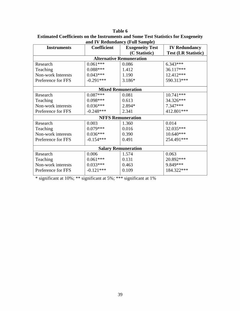
39

Table 6 Estimated Coefficients on the Instruments and Some Test Statistics for Exogeneity

and IV Redundancy (Full Sample) Instruments Coefficient Exogeneity Test

(C Statistic) IV Redundancy

Test (LR Statistic) Alternative Remuneration

Research Teaching Non-work Interests Preference for FFS

0.061*** 0.088*** 0.043*** -0.291***

0.086 1.412 1.190 3.186*

6.343*** 36.117*** 12.412*** 590.313***

Mixed Remuneration Research Teaching Non-work interests Preference for FFS

0.087*** 0.098*** 0.036*** -0.248***

0.081 0.613 2.894* 2.341

10.741*** 34.326*** 7.347*** 412.801***

NFFS Remuneration Research Teaching Non-work interests Preference for FFS

0.003 0.079*** 0.036*** -0.154***

1.360 0.016 0.390 0.491

0.014 32.035*** 10.640*** 254.491***

Salary Remuneration Research Teaching Non-work interests Preference for FFS

0.006 0.061*** 0.033*** -0.121***

1.574 0.131 0.463 0.109

0.063 20.892*** 9.849*** 184.322***

* significant at 10%; ** significant at 5%; *** significant at 1%