Do hedge funds yield greater risk-adjusted rate of returns than ...

DEGREE PROJECT, IN APPLIED MATHEMATICS AND INDUSTRIAL, FIRST LEVELECONOMICS

STOCKHOLM, SWEDEN 2014

Do hedge funds yield greaterrisk-adjusted rate of returns thanmutual funds?

A QUANTITATIVE STUDY COMPARING HEDGEFUNDS TO MUTUAL FUNDS AND HEDGE FUNDSTRATEGIES

OSCAR BÖRJESSON, SEBASTIAN HAQ

KTH ROYAL INSTITUTE OF TECHNOLOGY

SCI SCHOOL OF ENGINEERING SCIENCES

Do hedge funds yield greater risk-adjusted rate of returns than mutual funds? A quantitative study comparing hedge funds to mutual funds and hedge fund strategies

O S C A R B Ö R J E S S O N S E B A S T I A N H A Q

Degree Project in Applied Mathematics and Industrial Economics (15 credits)

Degree Progr. in Industrial Engineering and Management (300 credits) Royal Institute of Technology year 2014

Supervisor at KTH was Camilla Johansson Landén Examiner was Tatjana Pavlenko

TRITA-MAT-K 2014:04 ISRN-KTH/MAT/K--14/04--SE Royal Institute of Technology School of Engineering Sciences KTH SCI SE-100 44 Stockholm, Sweden URL: www.kth.se/sci

Do hedge funds yield greater risk-adjusted rate of returns than mutual funds?A quantitative study comparing hedge funds to mutual funds and hedge fund strategies

Abstract

In recent times, the popularity of hedge funds has un-doubtedly increased. There are shared opinions on whetherhedge funds generate absolute rates of returns and whetherthey provide a strong alternative investment to mutualfunds. This thesis aims to examine whether hedge fundswith different investment strategies create absolute returnsand if certain investment strategies outperform others. Thisthesis compares hedge funds risk-adjusted rate of return to-wards mutual funds, such as mutual funds, to see if certaininvestment strategies are more lucrative than the corre-sponding investments in terms of excess returns to corre-sponding indices. An econometric approach was applied tosearch for significant differences in risk-adjusted returns ofhedge funds in contrast to mutual funds.

Our results show that Swedish hedge funds do not gen-erate as high risk-adjusted returns as Swedish mutual funds.In regard to the best performing hedge fund strategy, theresults are inconclusive. Also, we do not find any evidencethat hedge funds violate the effective market hypothesis.

Keywords: hedge fund, absolute returns, hedge fund strate-gies, regression analysis, mutual funds, risk-adjusted re-turn, Sharpe ratio, Effective market hypothesis

JEL classification: G10; G11; G12; G15; G23

2

Avkastar hedgefonder hogre risk-justerade avkastningar an aktiefonder?En kvantitativ studie som jamfor hedgefonder med aktiefonder och investeringsstrategier

Sammanfattning

Hedgefonder har den senaste tiden okat i popularitet.Samtidigt finns det delade meningar huruvida hedgefondergenererar absolutavkastning och om de fungerar som braalternativ till traditionella fonder. Denna uppsats syftar tillatt undersoka huruvida hedgefonder skapar absolutavkast-ning samt om det finns investeringsstrategier som preste-rar battre an andra. Denna uppsats jamfor hedgefondersriskjusterade avkastning med traditionella fonder, for attpa satt se om en viss investeringsstrategi ar mer lukrativi termer av overavkastning i forhallande till motsvarandeindex. Vi har anvant ekonometriska metoder for att sokaefter statistiskt signifikanta skillnader mellan avkastningenfor hedgefonder och traditionella fonder.

Vara resultat visar att svenska hedgefonder inte gene-rerar hogre risk-justerade avkastningar an svenska aktie-fonder. Vara resultat visar inga signifikanta skillnader vadgaller avkastning mellan olika strategier. Slutligen finner viheller inga bevis for att hedgefonder gar emot den effektivamarknadshypotesen.

Nyckelord: hedgefond, absolutavkastning, hedgefondsstra-tegier, regressionsanalys, aktiefond, riskjusterad avkastning,Sharpekvot, Effektiva marknadsteorin

JEL classification: G10; G11; G12; G15; G23

3

Acknowledgements

We would like to express our outmost gratitude to our supervi-sor Camilla Landen, who supplied us with different viewpointsto sucessfully tackle difficulities. We also would like to take thechance to thank Anna Jerbrant and Anneli Linde for assistingand providing us with guidance during the course of this work.In addition we would like to thank Rickard Olsson for providingus with literature, previous studies and some initial guidelines.

We are also very grateful to Christian Carping, and Ulf Bergand Krister Sjoblom for providing enlightening insights into thehedge funds industry. We were given a contrasted view to thenormally rather stringent academic viewpoint of the finance in-dustry.

Stockholm, 26th May, 2014

4

Contents

1 Introduction 81.1 Problem background . . . . . . . . . . . . . . . . . . . . . . . . . . . . . . 81.2 Problem statement . . . . . . . . . . . . . . . . . . . . . . . . . . . . . . . 81.3 Aim . . . . . . . . . . . . . . . . . . . . . . . . . . . . . . . . . . . . . . . 81.4 Limitations . . . . . . . . . . . . . . . . . . . . . . . . . . . . . . . . . . . 81.5 Methodology . . . . . . . . . . . . . . . . . . . . . . . . . . . . . . . . . . 9

1.5.1 Literature studies . . . . . . . . . . . . . . . . . . . . . . . . . . . . 91.5.2 Interviews . . . . . . . . . . . . . . . . . . . . . . . . . . . . . . . . 91.5.3 Statistical calculations . . . . . . . . . . . . . . . . . . . . . . . . . 9

2 Theoretical framework 102.1 Effective market hypothesis . . . . . . . . . . . . . . . . . . . . . . . . . . 102.2 Sharpe ratio . . . . . . . . . . . . . . . . . . . . . . . . . . . . . . . . . . . 102.3 Jensen’s alpha . . . . . . . . . . . . . . . . . . . . . . . . . . . . . . . . . . 102.4 Benchmark selection . . . . . . . . . . . . . . . . . . . . . . . . . . . . . . 112.5 Difference between hedge funds and mutual funds . . . . . . . . . . . . . . 112.6 Hedge fund investment strategies . . . . . . . . . . . . . . . . . . . . . . . 12

2.6.1 Long/short strategies . . . . . . . . . . . . . . . . . . . . . . . . . 122.6.2 Relative value strategies . . . . . . . . . . . . . . . . . . . . . . . . 122.6.3 Event-driven strategies . . . . . . . . . . . . . . . . . . . . . . . . . 122.6.4 Global macro strategies . . . . . . . . . . . . . . . . . . . . . . . . 12

2.7 Previous studies . . . . . . . . . . . . . . . . . . . . . . . . . . . . . . . . 132.7.1 Hedge funds vs mutual funds . . . . . . . . . . . . . . . . . . . . . 132.7.2 Hedge fund investment strategies . . . . . . . . . . . . . . . . . . . 14

3 Mathematical theory 153.1 Linear regression model . . . . . . . . . . . . . . . . . . . . . . . . . . . . 15

3.1.1 Key assumptions: . . . . . . . . . . . . . . . . . . . . . . . . . . . . 153.1.2 R2 and Adjusted-R2 . . . . . . . . . . . . . . . . . . . . . . . . . . 153.1.3 F-statistic & t-test . . . . . . . . . . . . . . . . . . . . . . . . . . . 16

3.2 Probit model & maximum likelihood . . . . . . . . . . . . . . . . . . . . . 173.2.1 Pseudo-R2 . . . . . . . . . . . . . . . . . . . . . . . . . . . . . . . . 17

3.3 Stepwise regression & backward elimination method . . . . . . . . . . . . 183.3.1 Bayesian Information Criterion (BIC) . . . . . . . . . . . . . . . . 183.3.2 Akaike Information Criterion (AIC) . . . . . . . . . . . . . . . . . 18

3.4 Heteroskedasticity . . . . . . . . . . . . . . . . . . . . . . . . . . . . . . . 183.5 Correction for heteroskedasticity . . . . . . . . . . . . . . . . . . . . . . . 183.6 Multicollinearity . . . . . . . . . . . . . . . . . . . . . . . . . . . . . . . . 193.7 Endogeneity . . . . . . . . . . . . . . . . . . . . . . . . . . . . . . . . . . . 193.8 Shapiro-Wilk test . . . . . . . . . . . . . . . . . . . . . . . . . . . . . . . . 19

4 Data management 204.1 Collection of data . . . . . . . . . . . . . . . . . . . . . . . . . . . . . . . . 204.2 Sample selection . . . . . . . . . . . . . . . . . . . . . . . . . . . . . . . . 204.3 Descriptive statistics . . . . . . . . . . . . . . . . . . . . . . . . . . . . . . 214.4 Variable specification . . . . . . . . . . . . . . . . . . . . . . . . . . . . . . 214.5 Potential biases . . . . . . . . . . . . . . . . . . . . . . . . . . . . . . . . . 23

4.5.1 Survivorship biases . . . . . . . . . . . . . . . . . . . . . . . . . . . 23

5

4.5.2 Self selection bias . . . . . . . . . . . . . . . . . . . . . . . . . . . . 234.5.3 Back-filing bias . . . . . . . . . . . . . . . . . . . . . . . . . . . . . 23

5 Regression models 245.1 Model 1 - Multiple linear regression model . . . . . . . . . . . . . . . . . . 245.2 Model 2 - Improved Multiple Regression model . . . . . . . . . . . . . . . 26

5.2.1 Model 2a . . . . . . . . . . . . . . . . . . . . . . . . . . . . . . . . 265.2.2 Model 2b . . . . . . . . . . . . . . . . . . . . . . . . . . . . . . . . 28

5.3 Model 3 - Final models . . . . . . . . . . . . . . . . . . . . . . . . . . . . . 305.3.1 Model 3a . . . . . . . . . . . . . . . . . . . . . . . . . . . . . . . . 305.3.2 Model 3b . . . . . . . . . . . . . . . . . . . . . . . . . . . . . . . . 31

5.4 Model 4 - Probabilistic regression model . . . . . . . . . . . . . . . . . . . 33

6 Empirical results 34

7 Analysis 367.1 Econometric analysis . . . . . . . . . . . . . . . . . . . . . . . . . . . . . . 367.2 Threats to internal validity . . . . . . . . . . . . . . . . . . . . . . . . . . 37

7.2.1 Sample selection bias . . . . . . . . . . . . . . . . . . . . . . . . . . 377.2.2 Omitted variables bias . . . . . . . . . . . . . . . . . . . . . . . . . 377.2.3 Simultaneous causality bias . . . . . . . . . . . . . . . . . . . . . . 38

8 Adherence to Effective Market Hypothesis 398.1 Empirical findings . . . . . . . . . . . . . . . . . . . . . . . . . . . . . . . 398.2 Inference . . . . . . . . . . . . . . . . . . . . . . . . . . . . . . . . . . . . . 39

9 Preferred investment strategy 419.1 Inferences from interviews . . . . . . . . . . . . . . . . . . . . . . . . . . . 41

10 Conclusions 43

11 Future research 43

References 44

Appendices 45

6

List of Tables

1 Difference hedge funds and mutual funds . . . . . . . . . . . . . . . . . . 112 Descriptive statistics . . . . . . . . . . . . . . . . . . . . . . . . . . . . . . 213 Model 1 fit . . . . . . . . . . . . . . . . . . . . . . . . . . . . . . . . . . . 244 VIF results for Model 1 . . . . . . . . . . . . . . . . . . . . . . . . . . . . 255 Correlation matrix - Key independent variables . . . . . . . . . . . . . . 256 Shapiro-Wilk test Model 1 . . . . . . . . . . . . . . . . . . . . . . . . . . 257 Model 2a fit . . . . . . . . . . . . . . . . . . . . . . . . . . . . . . . . . . 268 VIF results for Model 2a . . . . . . . . . . . . . . . . . . . . . . . . . . . 279 AIC/BIC for Model 2a . . . . . . . . . . . . . . . . . . . . . . . . . . . . 2710 Shapiro-Wilk test Model 2a . . . . . . . . . . . . . . . . . . . . . . . . . . 2711 Model 2b fit . . . . . . . . . . . . . . . . . . . . . . . . . . . . . . . . . . 2812 VIF results for Model 2b . . . . . . . . . . . . . . . . . . . . . . . . . . . . 2913 AIC/BIC for Model 2b . . . . . . . . . . . . . . . . . . . . . . . . . . . . . 2914 Shapiro-Wilk test model 2b . . . . . . . . . . . . . . . . . . . . . . . . . . 2915 KIID Correlation matrix 3a . . . . . . . . . . . . . . . . . . . . . . . . . . 3016 Model 3a fit . . . . . . . . . . . . . . . . . . . . . . . . . . . . . . . . . . 3017 VIF results for Model 3a . . . . . . . . . . . . . . . . . . . . . . . . . . . 3118 Shapiro-Wilk test Model 3a . . . . . . . . . . . . . . . . . . . . . . . . . . 3119 Correlation matrix - KIID . . . . . . . . . . . . . . . . . . . . . . . . . . 3120 Model 3b fit . . . . . . . . . . . . . . . . . . . . . . . . . . . . . . . . . . 3221 VIF results for Model 3b . . . . . . . . . . . . . . . . . . . . . . . . . . . 3222 Shapiro-Wilk test Model 3b . . . . . . . . . . . . . . . . . . . . . . . . . . 3323 Model 4 fit . . . . . . . . . . . . . . . . . . . . . . . . . . . . . . . . . . . 3324 VIF results for Model 4 . . . . . . . . . . . . . . . . . . . . . . . . . . . . 3425 Estimation results - Regression of covariates on Sharpe ratio . . . . . . . 3526 Index for hedge funds and stock market . . . . . . . . . . . . . . . . . . . 3927 Distribution of Hedge fund strategies . . . . . . . . . . . . . . . . . . . . . 4228 Estimation results for Model 1 . . . . . . . . . . . . . . . . . . . . . . . . 4529 Estimation results for Model 2a . . . . . . . . . . . . . . . . . . . . . . . 4630 Estimation results for Model 2b . . . . . . . . . . . . . . . . . . . . . . . 4631 Estimation results for Model 3a . . . . . . . . . . . . . . . . . . . . . . . 4732 Estimation results for Model 3b . . . . . . . . . . . . . . . . . . . . . . . 4733 Estimation results for Model 4 . . . . . . . . . . . . . . . . . . . . . . . . 48

List of Figures

1 Residual plots for Model 1 . . . . . . . . . . . . . . . . . . . . . . . . . . . 482 Residual plots for Model 2a . . . . . . . . . . . . . . . . . . . . . . . . . . 493 Residual plots for Model 2b . . . . . . . . . . . . . . . . . . . . . . . . . . 494 Residual plots for Model 3a . . . . . . . . . . . . . . . . . . . . . . . . . . 505 Residual plots for Model 3b . . . . . . . . . . . . . . . . . . . . . . . . . . 50

7

1 Introduction

↪→ In this section we give the problem background and introduce the problem formulation,i.e. which questions this thesis aims to answer. We then write about the limitations andmethodology.

1.1 Problem background

Hedge funds often use complex investment strategies to succeed in generating absolutereturns1 and have unconstrained allocation rules in contrast to mutual funds. This resultsin fund managers having greater possibilities to take speculative positions on the market.The word “hedge” in hedge funds refers to the fact that hedge funds traditionally tendto use hedging techniques. However hedge funds do not have to engage in these types ofpractices. Hedge funds are often not as regulated as the corresponding mutual funds andthey therefore often bypass different types of licensing requirements that are applicableto other types of funds, such as mutual funds. In recent years, increased popularity ofhedge funds has made it into one of the main investment products and also one of thelargest sources of capital.

1.2 Problem statement

Due to the increased popularity of hedge funds, there are reasons to fully investigatewhether hedge funds in fact does reach their goals of generating stable positive returns.In order to conduct such an investigation, this thesis attempts to answer the followingquestions:

• Does hedge funds yield greater risk-adjusted returns than mutual funds?

• Is there an investment strategy which is used more frequently than others?

• Can Swedish hedge funds’ returns be explained by the effective market hypothesis?

1.3 Aim

This report aims to investigate the difference in risk-adjusted return for hedge funds andmutual funds, what hedge fund strategy is the preferred strategy among Swedish hedgefund managers and also if the effective market hypothesis can be used to explain thereturn of hedge funds. The aim is to provide an insight into the Swedish hedge fundindustry. The results could be used to motivate the use of certain hedge fund strategies.

1.4 Limitations

This thesis will concentrate on funds with Sweden as legal domicile. Furthermore, we havechosen to focus on four dominant hedge fund strategies in such way that other strategiesmight be categorized under our strategies of choice. We have also chosen the time periodbetween 2011 and 2014. This is in order to get results that show how the funds performduring “neutral” market conditions. For hedge funds, an interesting question is of courseif they generate stable and positive returns during financially distressed periods. This ishowever beyond the scope of this thesis, since the question is if hedge funds can outperformmutual funds during ordinary market circumstances.

1http://www.investopedia.com/terms/a/absolutereturn.asp

8

1.5 Methodology

In order to successfully conduct the investigation and analysis, this thesis will use thefollowing three methods:

1.5.1 Literature studies

We have studied scientific literature in order to get a deeper understanding of differenthedge fund strategies. Several studies of hedge funds in relation to mutual funds havebeen made. However, none has been made for Swedish markets. The scientific studies arediscussed in detail in Section 2.7.

The papers used in this thesis were found using the KTH library search function forpublications. The search words were “hedge funds” and ”hedge fund strategies” with thetopics: “hedge funds”, “hedge fund” and “performance” and ”hedge fund strategies” ,”performance” and ”hedge funds”, respectively. The search only included peer-reviewedmaterial and the papers chosen were those considered the most relevant.

1.5.2 Interviews

In order to understand how certain Swedish hedge fund managers allocate capital in dif-ferent funds, we interviewed three fund managers from two different hedge funds. Thisalso provided another point of view, complementing scientific studies, since theoreticaljustifications might be different for practical purposes. The selection of interview candi-dates were made by contacting fund managers through mail, inviting them to meet withus for a interview. The fund managers that responded were interviewed. The interviewswere conducted as open conversations with hedge fund strategies as the only guideline.

1.5.3 Statistical calculations

The statistical methods include calculations that examines whether hedge funds outper-forms mutual funds with the use of regression analysis. We improve on an initial model byusing different criterion. We also use statistical tools that alleviates problems that mightoccur between models. The calculations will be based on the Morningstar database forSwedish mutual and hedge funds.

9

2 Theoretical framework

↪→ This section provides the theoretical framework for understanding the specification ofthe regression model. It consists of theory within the field of corporate finance as well asclassification of different hedge fund strategies and finally previous studies.

2.1 Effective market hypothesis

The efficient market hypothesis states that the price of all securities is fair, based on futurecash flow, given all the information that is available to investors. This means that it isnot possible to constantly outperform corresponding market indices with the informationavailable to all investors. The information available to all investors is information foundin news reports, financial statements, corporate press releases or information from otherdata sources.[1]

The reasoning behind the efficient market hypothesis is that investors are expected tobe very competitive and therefore the market should react instantaneously to new infor-mation concerning a security, meaning that the price of said security should converge tothe “true” price in a short time period.

Eugene Fama is the originator of the EMH and therefore supports passive management,i.e. management through index. He believes that the stock market reacts on all informa-tion at such a fast pace that it is not possible to choose stocks that are better than theaverage. Robert Schiller, on the other hand, agrees with Fama’s theory that the stockmarket is effective on the short run. However, he shows that there are possibilities for anactive manager to beat stock market indices on the long run2.

2.2 Sharpe ratio

The Sharpe ratio is the ratio between the excess return of an asset and the asset’s volatility.The excess return is in this case the return of the asset minus the return of a benchmarkasset e.g. an index or the risk-free interest rate. In other words, the Sharpe ratio de-scribes the compensation investors get for taking a risk. The Sharpe ratio can be usedto compare different assets with a common benchmark asset, the asset with the highestSharpe ratio provides either higher return for the same risk or the same return for lowerrisk. The Sharpe ratio can also be used as an instrument to measure the performance ofan investment [1].

Sharperatio =ExcessReturn

V olatility=E(ra − rf )

σa(1)

According to equation (1) the Sharp ratio is calculated as the difference between the rateof return of the asset and a benchmark asset divided by the standard deviation of thedifference, in accordance with the Morningstar definition.

2.3 Jensen’s alpha

Jensen’s alpha is best described as a risk-adjusted measure of a portfolio’s performance, orreturn on an investment created by active management. Thus, it estimates the contribu-tions to a fund’s return that is actively created by a manager, or the managers predictive

2http://www.kva.se/Documents/Priser/Ekonomi/2013/pop_en_13.pdf

10

abilities. This risk-adjusted measure is used to predict the returns that are created inexcess of a corresponding passively managed portfolio given a certain risk level. In orderto access the relative performance, a benchmark is often subtracted from the performance,in order to achieve Jensen’s alpha [2].

It is normally argued that the expected value of alpha is zero, E(α) = 0, in an effi-cient market. According to this setting, alpha can be used to measure the performance ofan asset based on the risk it has taken. A manager with strong ability to predict markettiming will have a significantly positive α due to consistent positive residuals. In the samemanner, a manager that consistely achivies lower performance will have a significantlynegative α.[1]

2.4 Benchmark selection

Benchmarks can be best described as an objective standard used for the comparisonand evaluation of the performance of an asset. The importance of choosing the correctbenchmark for an asset lies in that it must, in an adequate manner, reflect the particularstyle that an investment manager uses. Since hedge funds does not explictly make use ofbenchmarks as comparison tools for evaluating performance, we choose the risk-free rate ofinterest, 10 year Swedish government bond3. In order to make a fair comparison betweenhedge funds and mutual funds, the risk-free rate of return is used as a benchmark forboth fund types. Since, the two fund types have different aims, the benchmark selectioncan be questioned. However, this will be discussed more in detail in the analysis.

2.5 Difference between hedge funds and mutual funds

The table below describes the common features of hedge funds and mutual funds, thuspresenting the differences of the fund types. Hedge fund placements rules are normally

Table 1: Difference hedge funds and mutual funds

Hedge funds Mutual Funds

Placement rules Free Limited

Return target Absolute return Relative returns

Outlook on risk Lose money Deviate from index

Investment philosophy Limit market risks by combin-ing long and short positions

Market risk by taking longpositions

Measure of success High yield compared to risk Exceed market index

Fee system Fixed and performance-based Fixed

Fund manager investments Very common Uncommon

much more free than mutual funds. Hedge funds can take positions in different financialderivatives in order to increase their returns, whereas mutual funds often subjected tostrict regulations which allows them only to take long positions and therefore the riskexposure normally is in form of market risk.[3]

3http://www.riksbank.se/sv/Rantor-och-valutakurser/

11

2.6 Hedge fund investment strategies

Hedge funds can best be described as investment vehicles that are speculative in natureand designed to take advantage of information that is held by the hedge fund managers.It is in the hands of the fund manager to decide when the information is no longeruseful in terms of making trades, and only then will it not be kept a secret. Hedge fundmanagers are therefore, quite reasonably, also reluctant to revealing information aboutinvestment strategies, since this might turn out to uncover essential information aboutdifferent positions that hedge funds are likely to take. The major investment strategies canbe outlined into four categories based on what type of positions the hedge funds engagein. Independent of the strategy, it is of vast importance that hedge funds have a lowcorrelation with the financial markets. This is essential since hedge funds should remainstable during economic recessions4. The descriptions of the four different strategies beloware based on An Introduction to Hedge Funds, Introductory Guide [4].

2.6.1 Long/short strategies

One of the most common strategies is the long/short strategy. This strategy involvestaking long or short positions, where taking short positions refers to hedge fund managersusing the strategy of selling securities that are not currently possessed by the fund. Thisallows them, unlike mutual funds, to speculate in the price falls. Strategies involvingtaking long and short positions separate market risk from the risk of the individual stock.

2.6.2 Relative value strategies

The relative value strategies are used to exploit arbitrage opportunities. These strategiestrust that mispriced securities will return to their intrinsic value in the long run, howeverwith deviations in the short run that will open up opportunities for profit. There areseveral ways of exploiting arbitrage opportunities, and amongst them are: convertiblearbitrage, capital arbitrage, fixed income arbitrage, yield curve arbitrage and corporatespread arbitrage. The underlying principle is that the market has in some way mispricedan asset or asset class, relative to other assets, and with the assumption that in the longrun the market will move back to equilibrium levels, short-term profits can be made.

2.6.3 Event-driven strategies

Event-driven strategies are highly speculative in nature. They rely on an approach thatis based on events that will influence the market during a short period of time. Examplesof an event that affects the market might be stock buybacks or earnings surprises. Thishedge fund strategy also relies on that hedge fund managers are in possession of superiorinformation that can be exploited in order to make stronger returns. An event drivenstrategy that is commonly used amongst hedge funds are distressed securities investing,which implies that hedge funds takes long positions in securities that are currently ex-periencing financial problems, such as firms that have filed for credit protection or arepriced over their intrinsic value in contrast to counterparts in the same industry.

2.6.4 Global macro strategies

In tactical strategies of trading, the main objective is to forecast the direction of themarket movements and thus forecasting the profits of the securities of a certain industry.

4http://www.brummer.se/sv/Om-oss/Vad-ar-hedgefond/

12

In this type of strategy, the timing of entering certain positions as well as how well thefund manager can predict the price movements in an industry is of great importance.One often-used strategy is the pure macro strategy that involves taking advantage ofmacroeconomic events such as a change in stock market performance, interest rates ormarket trends. Hedge funds that engage in macro strategies extensively use financialderivatives as well as leverage in order to forecast major economic trends and then investin asset classes or certain countries where an investment opportunity can be found.

2.7 Previous studies

2.7.1 Hedge funds vs mutual funds

Due to hedge funds growing popularity, they have been under quite hefty scrutiny. Manyinvestors consider hedge funds an alternative investment to traditional stocks and bonds.Thus, in recent times, the number of articles that discuss whether hedge funds have ahigher risk-adjusted performance than mutual funds has increased drastically.

Ackerman, McEnally, Ravenscraft (1999) compare hedge funds to mutual funds in termsof risk-adjusted performance and Sharpe ratio in their paper The Performance of Hedgefunds: Risk, Return, and Incentives. They find that hedge funds consistently outper-form mutual funds. They also compare hedge funds to standard market indices and theyconclude that market indices are not outperformed. Amongst the conclusions are alsothat hedge funds are more volatile than both market indices and corresponding mutualfunds. Incentive fees can, to some extent, explain hedge fund performance. However theincentive fees cannot explain the total risk taken by the portfolio [5].

Liang (1998) examines in the paper On the Performance of Hedge Funds the perfor-mance and risk of hedge funds during the period 1994-1996, and concludes that hedgefunds show a rather low correlation with financial markets and to other hedge funds. Thisis exemplary good for the diversification of a portfolio. Liang finally concludes that hedgefunds are better investment vehicle than mutual funds. This is because Liang showedthat hedge funds have a higher Sharpe ratio than mutual funds, and they generally showa higher performance rate relative to the remaining financial markets during the periodof examination [6].

Dichev and Yu (2011) compares the investor returns of hedge funds and buy-and-holdfund returns in their paper Higher risk, lower returns: What hedge fund investors reallyearn. Their main finding is that annualized dollar-weighed returns are 3-7% lower thanthe corresponding buy-and-hold funds. Also, using a factor model of risk and the esti-mated dollar-weighted performance gap they come to the conclusion that the real alphaof hedge fund investors is close to zero [7].

Capocci and Hubner (2004) investigate the performance of different hedge fund strate-gies using asset pricing models in their paper Analysis of hedge fund performance. UsingCAPM, Fama-French and Agarwal’s and Naik’s asset pricing models with the additionof a factor taking into account that some hedge funds invest in emerging market bonds,they come to the conclusion that one fourth of all hedge funds deliver significant positiveexcess returns and 10 of 13 strategies offer significantly positive return. They also findthat the best performing funds use momentum strategies, they do not invest in emergingmarkets and they prefer low-book-to-market stocks [8].

13

2.7.2 Hedge fund investment strategies

Brown, Goetzmann and Ibottson (1999) examine in their paper Offshore Hedge Funds:Survival and Performance how successful offshore hedge funds have been in terms ofJensen’s alpha. They categorize 10 different types of funds, and show that all the cate-gories show a positive alpha except short selling. In all cases, the alpha was statisticallysignificant. Since the examined hedge funds had a low correlation with the U.S. stockand bond market, the authors conclude that the hedge funds can be used for portfoliodiversification [9].

Olmo and Sanso-Navarro (2012) predict the relative performance of hedge fund investmentstrategies in their paper Forecasting the performance of hedge fund styles By using time-varying conditional stochastic dominance tests they forecast the return of hedge funds.More specifically they forecast the return of hedge funds during the recent financial crisisand come to the conclusion that global macro strategy outperform the other strategies.They also observe that different factors have more or less influence over the predictionsdepending on the region of the returns distribution and that the Fung and Hsieh factors(asset-based style factors) can be used for hedge fund return density forecasting [10].

Fung and Hsieh (2011) investigates the long/short strategy hedge funds in their paperThe risk in hedge fund strategies: Theory and evidence from long/short equity hedge funds.They find that less than 20% of the 3000 viewed long/short hedge funds were able to de-liver persistent and significant positive alpha. They also find that evidence point to alphadecaying over time. However, they don’t find evidence that support that size has a neg-ative effect on alpha. They also make a comment stating that, even though long/shortstrategies have a small representation of alpha performing funds, they still outperformequity mutual funds [11].

14

3 Mathematical theory

↪→ In this section, we introduce the statistical theory used for conducting the regressionanalysis. We also provide the theory for the methods used for optimizing our regressionmodels.

3.1 Linear regression model

The multiple linear regression model is specified according to:

yi =k∑

j=0

xijβj + ei, i = 1, ..., n (2)

where yi is the dependent random regressand for each observation, wheras the xij arecovariates. The regression coefficients are denoted βj and the error terms are denoted ei,which are assumed to be independent between observations. The multiple linear regressionmodel can compactly be written as:[12]

Y = Xβ + e (3)

where,

Y =

y1...yn

β =

β0...βk

e =

e0...en

X =

x1,0 x1,1 · · · x1,kx2,0 x2,1 · · · x2,k

......

. . ....

xn,0 xn,1 · · · xn,k

3.1.1 Key assumptions:

These assumptions can be found more in detail in Introduction to econometrics [13].

1. The conditional distribution of ei given x1j , ..., xnj has a mean of zero.

2. x1j , ..., xnj for i = 1, 2, ..., .n are i.i.d.

3. Large outliers are unlikely.

4. There is no perfect multicollinearity.

3.1.2 R2 and Adjusted-R2

R2 and Adjusted-R2 are both used as measures of goodness of fit. According to the set-ting below y is the predicted value of y and y is the mean value of y.

15

R2 = 1−

N∑i=0

(yi − yi)

N∑i=0

(yi − yi)(4)

The adjusted-R2 is a modified version of R2 that takes into account the addition of anew variable. It can therefore either decrease or increase when adding a new variable,depending if the variable helps explain Y or not.

R2 = 1− n− 1

n− k − 1

N∑i=0

(yi − yi)

N∑i=0

(yi − yi)(5)

Equation (5) shows that the adjusted-R2 is 1 minus the ratio of the sample variance ofthe OLS residuals (with degree of freedom correction) to the sample variance of Y.[13]

3.1.3 F-statistic & t-test

The t-test is used to test the null hypothesis that an estimated covariate of the regressionmodel is equal to a constant. The t-statistic can be used when testing the null hypothesis,H0 : βi = 0. Under the null hypothesis t belongs to student’s t distribution with n−k−1degrees of freedom, with n being number of observations and k being number of covariatesin the regression model. The t-statistic is given by:

t =βi − βiSE(βi)

(6)

where βi is the estimated covariate, βi is the constant and SE(βi) is the standard errorof the estimated covariate i. The p-value for the null hypothesis is:

p = 2 Pr(T ≥ |t|) (7)

where T ∈ t(n− k − 1).

When testing the null hypothesis that several covariates are zero, the F-test is used.The F-statistic is given by:

F =n− k − 1

r

(|e∗|2

|e|2− 1

)(8)

where |e|2 is the sum of squared residuals for the full model and |e∗|2 is the sum of squaredresiduals for the model with the tested covariates set to zero, n and k is the same as forthe t-test and r is the number of tested covariates. The p-value of the null hypothesis is:

p = Pr(X > F ) (9)

where X ∈ F (r, n− k − 1). [12]

16

3.2 Probit model & maximum likelihood

For the probit model, the dependent variable Yi, i = 1, ..., n, is defined as a binary variable.The probability that Yi = 1, conditional on xi1, ..., xik, is calculated as pi = φ(β0 +β1xi1 + · · · + βkxik). The conditional probability distribution for the ith observation isPr(Yi|xi1, ..., xik) = pyii (1 − pi)1−yi . Assuming that (xi1, ..., xik, Yi) are i.i.d., i = 1, ..., n,the joint probability distribution of Y1, ..., Yn conditional on the covariates is

Pr(Y1 = y1, ..., Yn = yn|xi0, ..., xik, i = 1, ..., n)

= Pr(Y1 = y1|x10, ..., x1k × · · · × Pr(Yn = yn|xn0, ..., xnk)

= py11 (1− p1)1−y1 × · · · × pynn (1− pn)1−yn

(10)

The likelihood function is the joint probability distribution, treated as a function of theunknown coefficient. It is conventional to consider the logarithm of the likelihood.Accordingly, the log-likelihood function is:

ln[fprobit(β0, ..., βk;Y1, ..., Yn|x0i, ..., xki, i = 1, ..., n)]

=

n∑i=1

Yiln[φ(β0 + β1x1i + · · ·+ βkxki)]

+n∑

i=1

(1− yi)ln[1− φ(β0 + β1x1i + · · ·+ βkxki)]

(11)

where this expression incorporates the probit formula for the conditional probabiliy, pi =φ(β0 + β1x1i + · · · + βkxki). The MLE for the probit model maximizes the likelihoodfunction, or equivalently, the logarithm of the likelihood function given in equation above.Because there is no simple formula for the MLE, the probit likelihood function must bemaximized using a numerical algorithm. Under general conditions, maximum likelihoodestimators are consistent and have a normal sampling distribution in large samples.[13]

3.2.1 Pseudo-R2

In probit regression, pseudo R-squared are used, since probit regression does not have enequivalent to the usual R-squared used in OLS regression. Therefore McFadden’s pseudoR-squared is normally used:

R2 = 1−ln(L(Mf ))

ln(L(Mi))(12)

According to this setting, Mf is the model with predictors, and Mi is the model without

predictors, and L is the estimated likelihood. The log-likelihood of the intercept modelis treated as a total sum of squares and the log-likelihood of the full model is treated asthe sum of squared errors.[13]

17

3.3 Stepwise regression & backward elimination method

In order to find a regression model that is optimized for solving our thesis question, we usea stepwise regression method. Specifically will we use the backward elimination method.This method uses the particular procedure:

1. All covariates are included in our intial multiple linear regression model.

2. We test the deletion of each covariate from regression using the criterions.

3. We delete the covariates that improves the model most without losing explanatorypower, and then repeat this process until we cannot further improve our model.

We will use the stepwise regression method by two different criterions, namely theBayesian Information Criterion and teh Akaike Information Criterion.

3.3.1 Bayesian Information Criterion (BIC)

Regression models can be overfitted by having too many covariates. A common testfor this is the BIC (Bayesian Information Criterion) test. One chooses the model thatminimizes:

nln(∣∣e2∣∣) + kln(n) (13)

where k is the number of covariates (including the intercept) and n the number of obser-vations and |e2| is the sum of squares.[12]

3.3.2 Akaike Information Criterion (AIC)

In addition to BIC, there is another way of determining if a covariate should enter theequation, AIC (Akaike Information Criterion). AIC differs from BIC in the second term,where instead of ”ln(n)” there is ”2”. So the preferred model is the one that minimizes:

nln(∣∣e2∣∣) + 2k (14)

where k is the number of covariates (including the intercept), n the number of observationsand |e2| is the sum of squares.[13]

3.4 Heteroskedasticity

Heteroskedasticity is when the variance of the error terms differ between observations.For instance, an example of heterskedasticity is when the variance of the error termsdepend on the values of the covariates. Heteroskedasticity can be detected by plottingthe residuals against every covariate. If there is a correlation, then there are signs ofheteroskedasticity.[12]

3.5 Correction for heteroskedasticity

When computing the regressions in our statistical software, we use a setting allowing us tocorrect for heteroskadasticity. We get heteroscedascity robust standard errors accordingly.This is equivalent to White’s consistent variance estimator, which is defined accordingly:

18

Cov(β) = (XtX)−1XtD(e2)X(XtX)−1

= (XtX)−1

(n∑−1

e2ixtixi

)(XtX)−1

(15)

where D(e2) is the n× n diagonal matrix whose ith diagonal element is e2i .[12]

3.6 Multicollinearity

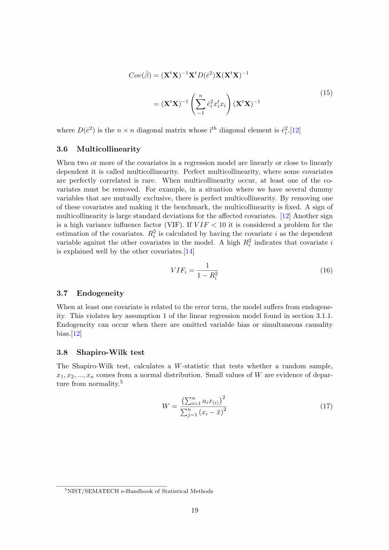
When two or more of the covariates in a regression model are linearly or close to linearlydependent it is called multicollinearity. Perfect multicollinearity, where some covariatesare perfectly correlated is rare. When multicollinearity occur, at least one of the co-variates must be removed. For example, in a situation where we have several dummyvariables that are mutually exclusive, there is perfect multicollinearity. By removing oneof these covariates and making it the benchmark, the multicollinearity is fixed. A sign ofmulticollinearity is large standard deviations for the affected covariates. [12] Another signis a high variance influence factor (VIF). If V IF < 10 it is considered a problem for theestimation of the covariates. R2

i is calculated by having the covariate i as the dependentvariable against the other covariates in the model. A high R2

i indicates that covariate iis explained well by the other covariates.[14]

V IFi =1

1−R2i

(16)

3.7 Endogeneity

When at least one covariate is related to the error term, the model suffers from endogene-ity. This violates key assumption 1 of the linear regression model found in section 3.1.1.Endogeneity can occur when there are omitted variable bias or simultaneous causalitybias.[12]

3.8 Shapiro-Wilk test

The Shapiro-Wilk test, calculates a W -statistic that tests whether a random sample,x1, x2, ..., xn comes from a normal distribution. Small values of W are evidence of depar-ture from normality.5

W =

(∑ni=1 aix(i)

)2∑nj=1 (xi − x)2

(17)

5NIST/SEMATECH e-Handbook of Statistical Methods

19

4 Data management

↪→ In this section we discuss the different data that is used and provide descriptive statis-tics for the dataset used for the regressions. We also discuss the different biases that occurin the dataset, and how they can be countered.

4.1 Collection of data

The data was collected from the Morningstar database, with own modifications such thatrelevant statistical test could be performed.

4.2 Sample selection

The data used in the regression is composed of 79 Swedish hedge funds and 405 Swedishmutual funds for a total of 484 funds, found at the Swedish Morningstar website. Sincethere, in Sweden, are quite few hedge funds, the total amount of data is very limited. Thislimitation affects the possibility to make restrictions when selecting data and therefore, inorder to have a sufficient amount of data, the hedge fund data for this report was selectedwith the sole restriction that they have to be Swedish. Because of limited data for eachfund the amount of hedge funds was reduced to 62 and the amount of mutual funds wasreduced to 291 for a total of 353 funds.

20

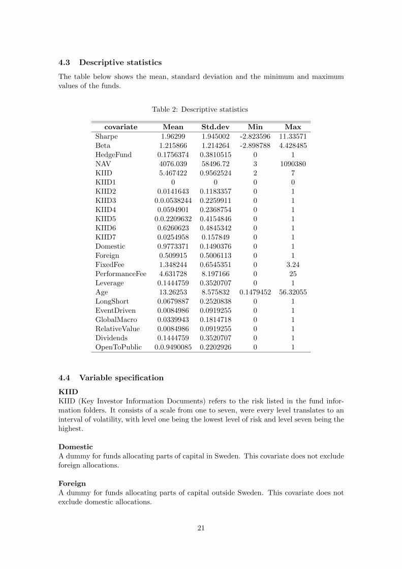
4.3 Descriptive statistics

The table below shows the mean, standard deviation and the minimum and maximumvalues of the funds.

Table 2: Descriptive statistics

covariate Mean Std.dev Min Max

Sharpe 1.96299 1.945002 -2.823596 11.33571Beta 1.215866 1.214264 -2.898788 4.428485HedgeFund 0.1756374 0.3810515 0 1NAV 4076.039 58496.72 3 1090380KIID 5.467422 0.9562524 2 7KIID1 0 0 0 0KIID2 0.0141643 0.1183357 0 1KIID3 0.0.0538244 0.2259911 0 1KIID4 0.0594901 0.2368754 0 1KIID5 0.0.2209632 0.4154846 0 1KIID6 0.6260623 0.4845342 0 1KIID7 0.0254958 0.157849 0 1Domestic 0.9773371 0.1490376 0 1Foreign 0.509915 0.5006113 0 1FixedFee 1.348244 0.6545351 0 3.24PerformanceFee 4.631728 8.197166 0 25Leverage 0.1444759 0.3520707 0 1Age 13.26253 8.575832 0.1479452 56.32055LongShort 0.0679887 0.2520838 0 1EventDriven 0.0084986 0.0919255 0 1GlobalMacro 0.0339943 0.1814718 0 1RelativeValue 0.0084986 0.0919255 0 1Dividends 0.1444759 0.3520707 0 1OpenToPublic 0.0.9490085 0.2202926 0 1

4.4 Variable specification

KIIDKIID (Key Investor Information Documents) refers to the risk listed in the fund infor-mation folders. It consists of a scale from one to seven, were every level translates to aninterval of volatility, with level one being the lowest level of risk and level seven being thehighest.

DomesticA dummy for funds allocating parts of capital in Sweden. This covariate does not excludeforeign allocations.

ForeignA dummy for funds allocating parts of capital outside Sweden. This covariate does notexclude domestic allocations.

21

FixedFeeThe fee the fund charges in order to run the fund. The investor is required to pay thisfee regardless of the fund’s performance. This fee is part of the model because a higherfee should mean a better performance since no one would pay a high fee for a bad product.

PerformanceFeeThe extra fee the fund charges if it outperforms its benchmark. It is listed in the data aspercent of result. This fee is part of the model because a performance fee should func-tion as an incentive for managers, therefore a higher performance fee should give greaterreturn. Also without the greater performance no one would invest in a fund with more fees.

LeverageA dummy variable describing whether the fund is allowed to use borrowed funds or not.Leverage is part of the model since it can enhance the returns of a fund if used wisely.

AgeThe age of the fund, listed in years.

HedgeFundA dummy variable which makes it possible to distinguish between mutual funds and hedgefunds.

LongShortA dummy variable describing if the hedge fund is using a long/short strategy or not.

EventdrivenA dummy variable describing if the hedge fund is using an event driven strategy or not.

GlobalMacroA dummy variable describing if the hedge fund is using a global macro strategy or not.

RelativeValueA dummy variable describing if the hedge fund is using a relative value strategy or not.

DividendDummy variable describing if the fund pays dividends or not. Dividends could help de-scribe the return of a fund because a dividend paying fund use less of its earnings to investin assets and should therefore have a smaller return.

OpenToPublicA dummy variable describing if the fund is open to the public or not. This could helpdescribe the return of a fund because of the difference in management and customer base.

NAVNet Asset Value for the fund, collected 2014-03-15.

MarketCorrA variable describing the market correlation of the funds.

22

StdDev3yThe funds standard deviation for the period 2011-03-15 to 2014-03-15. The variable mea-sures how much the funds performance has deviated in average during the last 36 monthsfrom the average return.

4.5 Potential biases

When collecting data in the fashion stated above there are several sources of potentialbiases. The most general of these, concerns the Morningstar data collection. It is hardto validate that the data collected at Morningstar is legitimate. But since Morningstar isa company with branches in several countries and with a mission to help investors reachtheir financial goals, any potential bias from them is unlikely since it would contradicttheir mission and the image of the company.

4.5.1 Survivorship biases

Survivorship bias is known to cause overstatement of performance because funds thatcease to trade are not included in the analysis, and these funds often have performedpoorly. This creates two problems in the case of hedge funds; fund survivorship and stylesurvivorship. Fund survivorship means overstatement of the true performance of hedgefunds. Style survivorship refers to the problem that the styles of surviving funds aredifferent from the styles of deceased funds.

4.5.2 Self selection bias

Contrary to mutual funds, hedge funds are not under the same regulations and thereforecan choose the start date of historical performance data. The only incentive for hedgefunds to report their performance, is to market their hedge funds. Obviously, hedge fundmanagers, have an incentive not to report data that impairs the image of the hedge fund.The result of self selection bias is then that the performance data shows better resultsthan the actual performance.

4.5.3 Back-filing bias

Another quite common source of bias is the back-filing bias, that essentially is createdwhen a new hedge fund is added to a database and is asked to provide, for instance,historical data for previous years. In cases when the hedge fund has rather averageyields, the hedge fund managers might refuse to supply the complete performance history.Instead, there is a rather strong incentive to hand over a shorter historical data of theperformance. The result is that the hedge fund shows a stronger performance than itactually has. In addition, the risk listed in the KIID is only representative for the lastfive years. This means that for example the financial crisis of 2008 will not be includedin the presented risk.

23

5 Regression models

↪→ In this section, the regression model is discussed as well as methods for evaluating thefit to data. We also show how the variability in the data is taken care of. By improvingour intial model, we will move towards a probit model that will allow us to calculate theprobability of a higher risk-adjusted rate of return given different hedge fund strategies.

5.1 Model 1 - Multiple linear regression model

In our first model, we employ a multiple linear regression model which includes all covari-ates in our dataset. By applying the theory of AIC/BIC we aim to improve the initialmodel, through the use of stepwise regression, more specifically, backward elimination.

Sharpei = β0

+ β1HedgeFund

+ β2StdDev3y

+ β3KIID

+ β4Domestic

+ β5Foreign

+ β6Age

+ β7FixedFee

+ β8PerformanceFee

+ β9Leverage

+ β10LongShorti

+ β11EventDriveni

+ β12GlobalMacroi

+ β13RelativeV aluei

+ β14Dividends

+ β15OpenToPublic

+ β16NAV

+ β17MarketCorr

+ ei

(18)

In Table 4 we see that HedgeFund has a VIF above the threshold of ten and the strategycovariates are slightly below ten. This indicates that there is multicollinearity betweenHedgeFund and the strategy covariates. Since these covariates are essential to our analy-sis this must be resolved. We do this by dividing the model into two separate models, onewith the HedgeFund covariate as well as all the other covariates exluding the strategycovariates and vice versa.

Table 3: Model 1 fit

Model Obs R2 Adjusted-R2 F(17,335) Prob. > F

Model 1 353 0.7714 0.7598 48.39 0.000

24

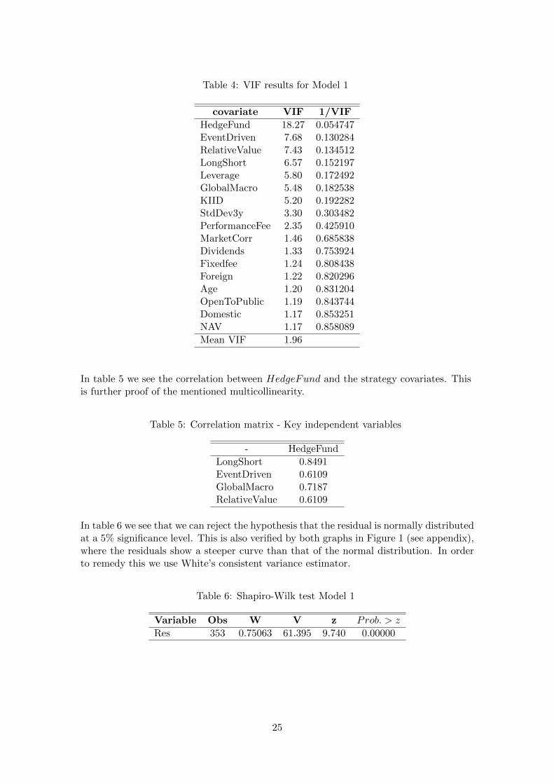
Table 4: VIF results for Model 1

covariate VIF 1/VIF

HedgeFund 18.27 0.054747EventDriven 7.68 0.130284RelativeValue 7.43 0.134512LongShort 6.57 0.152197Leverage 5.80 0.172492GlobalMacro 5.48 0.182538KIID 5.20 0.192282StdDev3y 3.30 0.303482PerformanceFee 2.35 0.425910MarketCorr 1.46 0.685838Dividends 1.33 0.753924Fixedfee 1.24 0.808438Foreign 1.22 0.820296Age 1.20 0.831204OpenToPublic 1.19 0.843744Domestic 1.17 0.853251NAV 1.17 0.858089

Mean VIF 1.96

In table 5 we see the correlation between HedgeFund and the strategy covariates. Thisis further proof of the mentioned multicollinearity.

Table 5: Correlation matrix - Key independent variables

- HedgeFund

LongShort 0.8491EventDriven 0.6109GlobalMacro 0.7187RelativeValue 0.6109

In table 6 we see that we can reject the hypothesis that the residual is normally distributedat a 5% significance level. This is also verified by both graphs in Figure 1 (see appendix),where the residuals show a steeper curve than that of the normal distribution. In orderto remedy this we use White’s consistent variance estimator.

Table 6: Shapiro-Wilk test Model 1

Variable Obs W V z Prob. > z

Res 353 0.75063 61.395 9.740 0.00000

25

5.2 Model 2 - Improved Multiple Regression model

5.2.1 Model 2a

As previously mentioned we do two sets of regression models. In this model the strategycovariates are excluded.

Sharpei = β0

+ β1HedgeFund

+ β2StdDev3y

+ β3KIID

+ β4Domestic

+ β5Foreign

+ β6Age

+ β7FixedFee

+ β8PerformanceFee

+ β9Leverage

+ β10Dividends

+ β11OpenToPublic

+ β12NAV

+ β13MarketCorr

+ ei

(19)

In table 7 we see that both R2 and adjusted-R2 has decreased slightly, this was to beexpected since the model has fewer explaining covariates. In table 8 we see that VIFis below the threshold of ten, for all covariates. This indicates that there is no multi-collinearity.

In table 9 we see that removing Dividends, Age, OpenToPublic, Domestic, Foreign,PerformanceFee and Leverage from the model will improve BIC and in most cases AICas well. Since low AIC and BIC indicate a better model these covariates are removed formodel 3a.

Table 7: Model 2a fit

Model Obs R2 AdjustedR2 F (13,339) Prob. > F

Model 2b 353 0.7611 0.7519 53.75 0.000

26

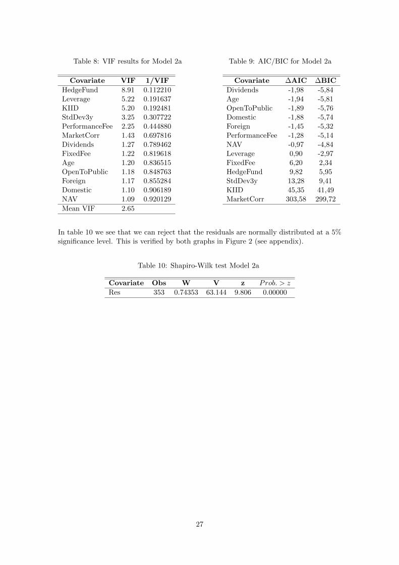
Table 8: VIF results for Model 2a

Covariate VIF 1/VIF

HedgeFund 8.91 0.112210Leverage 5.22 0.191637KIID 5.20 0.192481StdDev3y 3.25 0.307722PerformanceFee 2.25 0.444880MarketCorr 1.43 0.697816Dividends 1.27 0.789462FixedFee 1.22 0.819618Age 1.20 0.836515OpenToPublic 1.18 0.848763Foreign 1.17 0.855284Domestic 1.10 0.906189NAV 1.09 0.920129

Mean VIF 2.65

Table 9: AIC/BIC for Model 2a

Covariate ∆AIC ∆BIC

Dividends -1,98 -5,84Age -1,94 -5,81OpenToPublic -1,89 -5,76Domestic -1,88 -5,74Foreign -1,45 -5,32PerformanceFee -1,28 -5,14NAV -0,97 -4,84Leverage 0,90 -2,97FixedFee 6,20 2,34HedgeFund 9,82 5,95StdDev3y 13,28 9,41KIID 45,35 41,49MarketCorr 303,58 299,72

In table 10 we see that we can reject that the residuals are normally distributed at a 5%significance level. This is verified by both graphs in Figure 2 (see appendix).

Table 10: Shapiro-Wilk test Model 2a

Covariate Obs W V z Prob. > z

Res 353 0.74353 63.144 9.806 0.00000

27

5.2.2 Model 2b

In this model the covariate HedgeFund is excluded and since we only want to find differ-ence in performance caused by strategies, we exclude the mutual fund data. This leaveus with 62 observations.

Sharpei = β0

+ β1StdDev3y

+ β2KIID

+ β3Domestic

+ β4Foreign

+ β5Age

+ β6FixedFee

+ β7PerformanceFee

+ β8Leverage

+ β9LongShorti

+ β10EventDriveni

+ β11GlobalMacroi

+ β12RelativeV aluei

+ β13Dividends

+ β14OpenToPublic

+ β15NAV

+ β16MarketCorr

+ ei

(20)

In table 11 we see that both R2 and adjusted-R2 has decreased, which was expected sincecovariates were removed. In table 12 we see that VIF is well below the threshold for allcovariates and there is no sign of multicollinearity.

In table 13 we see that removing Leverage, Dividends, Foreign, OpenToPublic, NAV ,Domestic, Age and all the strategy covariates will improve BIC and in most cases AICas well. We therefore remove all these with the exception of the strategy covariates, weleave these in the model since they are key variables.

Table 11: Model 2b fit

Model Obs R2 AdjustedR2 F (16,45) Prob. > F

Model 2b 62 0.7387 0.6457 7.11 0.000

28

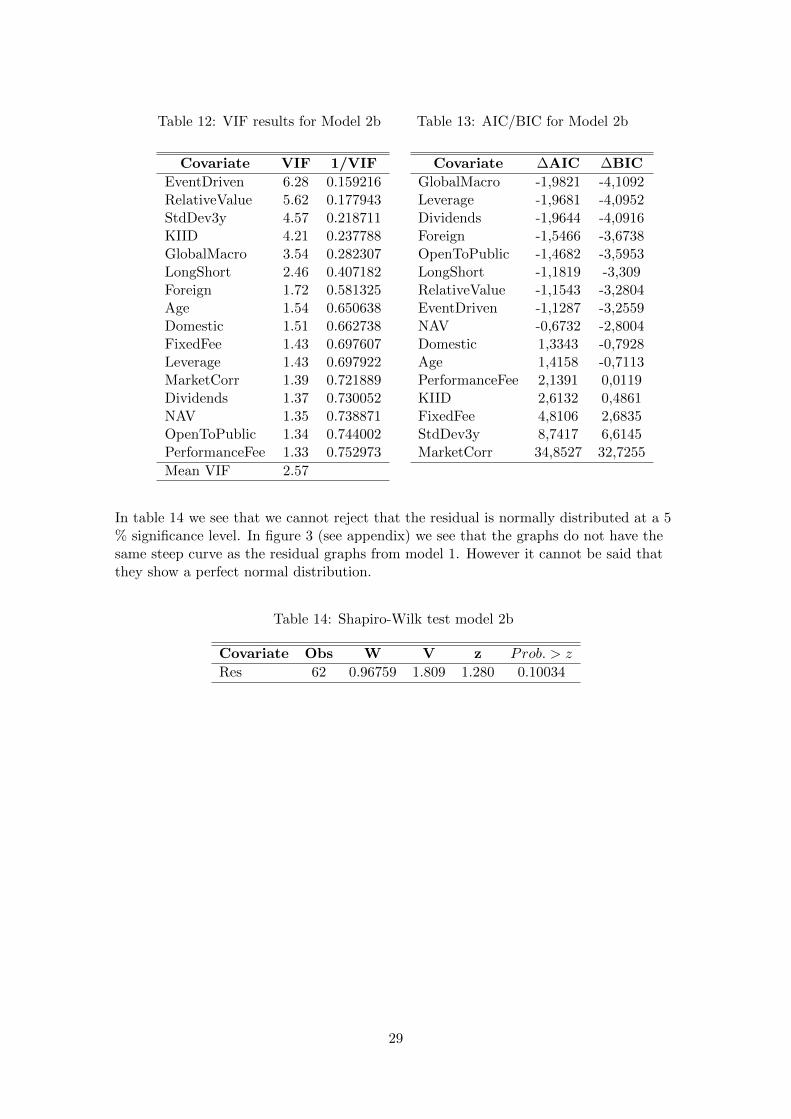
Table 12: VIF results for Model 2b

Covariate VIF 1/VIF

EventDriven 6.28 0.159216RelativeValue 5.62 0.177943StdDev3y 4.57 0.218711KIID 4.21 0.237788GlobalMacro 3.54 0.282307LongShort 2.46 0.407182Foreign 1.72 0.581325Age 1.54 0.650638Domestic 1.51 0.662738FixedFee 1.43 0.697607Leverage 1.43 0.697922MarketCorr 1.39 0.721889Dividends 1.37 0.730052NAV 1.35 0.738871OpenToPublic 1.34 0.744002PerformanceFee 1.33 0.752973

Mean VIF 2.57

Table 13: AIC/BIC for Model 2b

Covariate ∆AIC ∆BIC

GlobalMacro -1,9821 -4,1092Leverage -1,9681 -4,0952Dividends -1,9644 -4,0916Foreign -1,5466 -3,6738OpenToPublic -1,4682 -3,5953LongShort -1,1819 -3,309RelativeValue -1,1543 -3,2804EventDriven -1,1287 -3,2559NAV -0,6732 -2,8004Domestic 1,3343 -0,7928Age 1,4158 -0,7113PerformanceFee 2,1391 0,0119KIID 2,6132 0,4861FixedFee 4,8106 2,6835StdDev3y 8,7417 6,6145MarketCorr 34,8527 32,7255

In table 14 we see that we cannot reject that the residual is normally distributed at a 5% significance level. In figure 3 (see appendix) we see that the graphs do not have thesame steep curve as the residual graphs from model 1. However it cannot be said thatthey show a perfect normal distribution.

Table 14: Shapiro-Wilk test model 2b

Covariate Obs W V z Prob. > z

Res 62 0.96759 1.809 1.280 0.10034

29

5.3 Model 3 - Final models

Since KIID is divided in uneven intervals, (KIID7 represent 25% or more) we trans-form KIID into 7 dummy variables, each representing different KIID-levels. Since weuse different data for the different sets of regression models and we want to avoid multi-collinearity, we use different benchmarks for the different models. If two covariates showhigh correlation in comparison to the others, one of them will be chosen as benchmark.

5.3.1 Model 3a

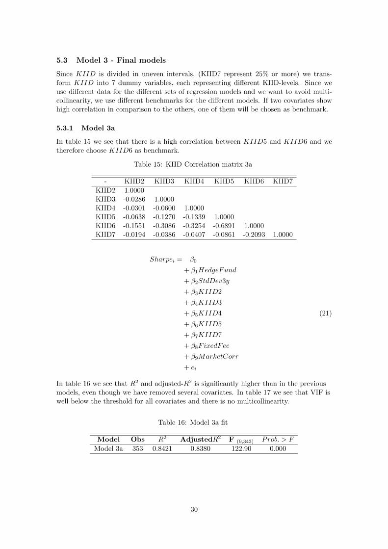
In table 15 we see that there is a high correlation between KIID5 and KIID6 and wetherefore choose KIID6 as benchmark.

Table 15: KIID Correlation matrix 3a

- KIID2 KIID3 KIID4 KIID5 KIID6 KIID7

KIID2 1.0000KIID3 -0.0286 1.0000KIID4 -0.0301 -0.0600 1.0000KIID5 -0.0638 -0.1270 -0.1339 1.0000KIID6 -0.1551 -0.3086 -0.3254 -0.6891 1.0000KIID7 -0.0194 -0.0386 -0.0407 -0.0861 -0.2093 1.0000

Sharpei = β0

+ β1HedgeFund

+ β2StdDev3y

+ β3KIID2

+ β4KIID3

+ β5KIID4

+ β6KIID5

+ β7KIID7

+ β8FixedFee

+ β9MarketCorr

+ ei

(21)

In table 16 we see that R2 and adjusted-R2 is significantly higher than in the previousmodels, even though we have removed several covariates. In table 17 we see that VIF iswell below the threshold for all covariates and there is no multicollinearity.

Table 16: Model 3a fit

Model Obs R2 AdjustedR2 F (9,343) Prob. > F

Model 3a 353 0.8421 0.8380 122.90 0.000

30

Table 17: VIF results for Model 3a

Covariate VIF 1/VIF

KIID3 3.46 0.288833HedgeFund 3.46 0.289012StdDev3y 3.30 0.303277KIID4 3.17 0.315628KIID5 1.91 0.524843KIID2 1.70 0.586574MarketCorr 1.41 0.708054FixedFee 1.27 0.786418KIID7 1.13 0.886676

Mean VIF 2.31

In table 18 we see that we can reject the hypothesis that the residual is normallydistributed. In figure 4 (see appendix) we see that the steepness of the curve hasincreased and is further from normal than the previous model.

Table 18: Shapiro-Wilk test Model 3a

Covariate Obs W V z Prob. > z

Res 353 0.75031 61.475 9.743 0.00000

5.3.2 Model 3b

In table 19 we see that KIID3 and KIID4 has the highest correlation and we thereforechoose KIID3 as benchmark.

Table 19: Correlation matrix - KIID

- KIID2 KIID3 KIID4 KIID5 KIID6

KIID2 1.0000KIID3 -0.1969 1.0000KIID4 -0.2044 -0.4587 1.0000KIID5 -0.1747 -0.3920 -0.4070 1.0000KIID6 -0.0541 -0.1214 -0.1260 -0.1077 1.0000

31

Sharpei = β0

+ β1StdDev3y

+ β2KIID2

+ β3KIID4

+ β4KIID5

+ β5KIID6

+ β6FixedFee

+ β7PerformanceFee

+ β8LongShorti

+ β9EventDriveni

+ β10GlobalMacroi

+ β11RelativeV aluei

+ β12MarketCorr

+ ei

(22)

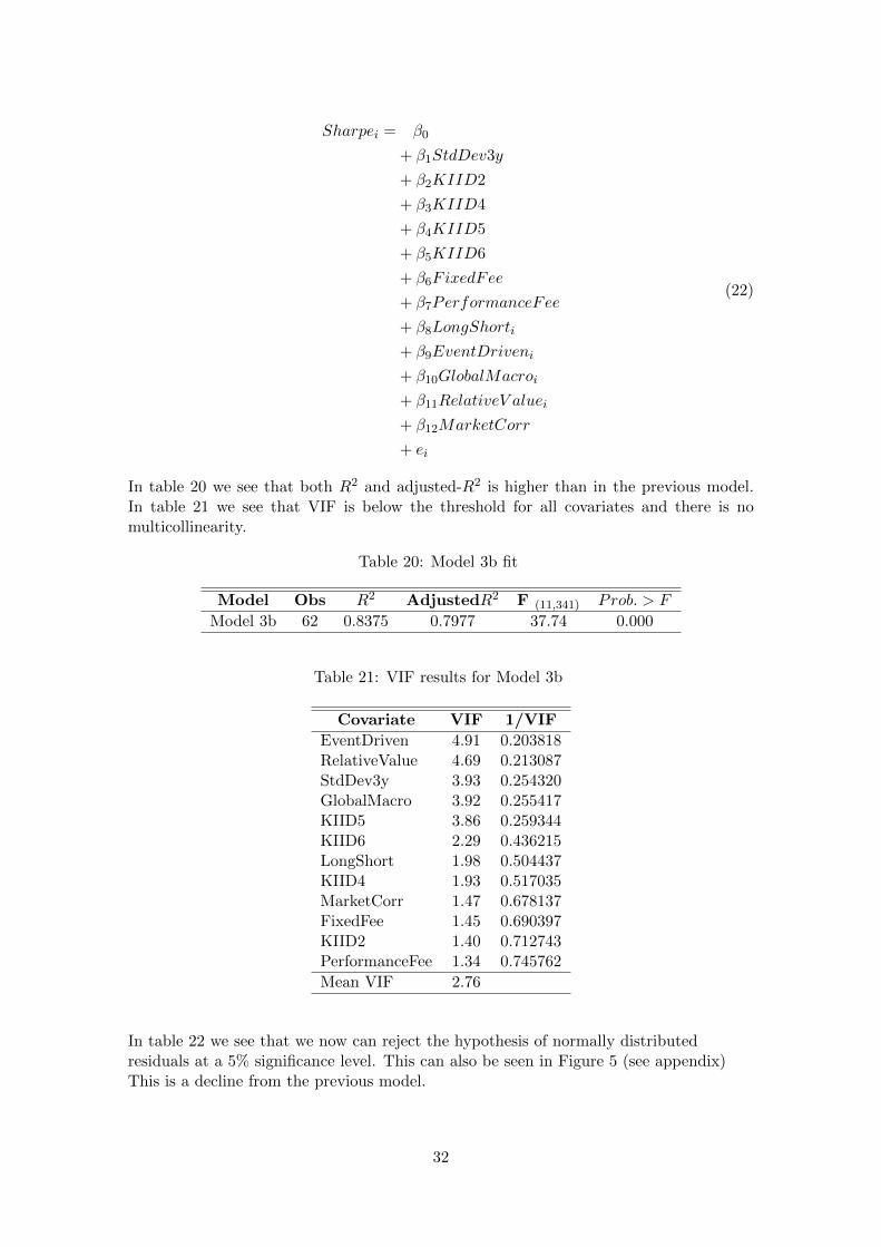
In table 20 we see that both R2 and adjusted-R2 is higher than in the previous model.In table 21 we see that VIF is below the threshold for all covariates and there is nomulticollinearity.

Table 20: Model 3b fit

Model Obs R2 AdjustedR2 F (11,341) Prob. > F

Model 3b 62 0.8375 0.7977 37.74 0.000

Table 21: VIF results for Model 3b

Covariate VIF 1/VIF

EventDriven 4.91 0.203818RelativeValue 4.69 0.213087StdDev3y 3.93 0.254320GlobalMacro 3.92 0.255417KIID5 3.86 0.259344KIID6 2.29 0.436215LongShort 1.98 0.504437KIID4 1.93 0.517035MarketCorr 1.47 0.678137FixedFee 1.45 0.690397KIID2 1.40 0.712743PerformanceFee 1.34 0.745762

Mean VIF 2.76

In table 22 we see that we now can reject the hypothesis of normally distributedresiduals at a 5% significance level. This can also be seen in Figure 5 (see appendix)This is a decline from the previous model.

32

Table 22: Shapiro-Wilk test Model 3b

Covariate Obs W V z Prob. > z

Res 62 0.94798 2.903 2.302 0.01068

5.4 Model 4 - Probabilistic regression model

For the probablistic model, a binary variable is defined, in the following way:

SharpeBin =

{1, if Sharpe ratio above 00, otherwise

Pr(SharpeBini|, β1StdDev3y

, β2KIID2

, β3KIID4

, β4KIID5

, β5KIID6

, β6KIID7

, β7FixedFee

, β8PerformanceFee

, β9LongShorti

, β10EventDriveni

, β11GlobalMacroi

, β12RelativeV aluei

, β13MarketCorr)

(23)

In this model some covariates were able to predict the dependent variable perfectly andthey were therefore omitted, which means that some observations were lost. This problemoccurs commonly in probit models, in our case due to few observations. In other words,there are variables that have same the values for the exact same observations.

Table 23: Model 4 fit

Model Obs Pseudo R2 Wald χ2(8) Prob. > χ2

(12)

Model 4 44 0.2638 275.68 0.000

33

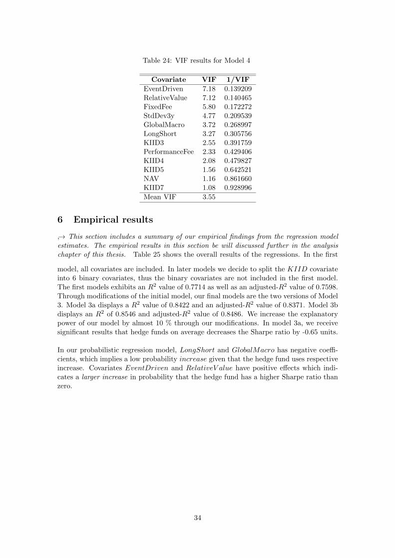
Table 24: VIF results for Model 4

Covariate VIF 1/VIF

EventDriven 7.18 0.139209RelativeValue 7.12 0.140465FixedFee 5.80 0.172272StdDev3y 4.77 0.209539GlobalMacro 3.72 0.268997LongShort 3.27 0.305756KIID3 2.55 0.391759PerformanceFee 2.33 0.429406KIID4 2.08 0.479827KIID5 1.56 0.642521NAV 1.16 0.861660KIID7 1.08 0.928996

Mean VIF 3.55

6 Empirical results

↪→ This section includes a summary of our empirical findings from the regression modelestimates. The empirical results in this section be will discussed further in the analysischapter of this thesis. Table 25 shows the overall results of the regressions. In the first

model, all covariates are included. In later models we decide to split the KIID covariateinto 6 binary covariates, thus the binary covariates are not included in the first model.The first models exhibits an R2 value of 0.7714 as well as an adjusted-R2 value of 0.7598.Through modifications of the initial model, our final models are the two versions of Model3. Model 3a displays a R2 value of 0.8422 and an adjusted-R2 value of 0.8371. Model 3bdisplays an R2 of 0.8546 and adjusted-R2 value of 0.8486. We increase the explanatorypower of our model by almost 10 % through our modifications. In model 3a, we receivesignificant results that hedge funds on average decreases the Sharpe ratio by -0.65 units.

In our probabilistic regression model, LongShort and GlobalMacro has negative coeffi-cients, which implies a low probability increase given that the hedge fund uses respectiveincrease. Covariates EventDriven and RelativeV alue have positive effects which indi-cates a larger increase in probability that the hedge fund has a higher Sharpe ratio thanzero.

34

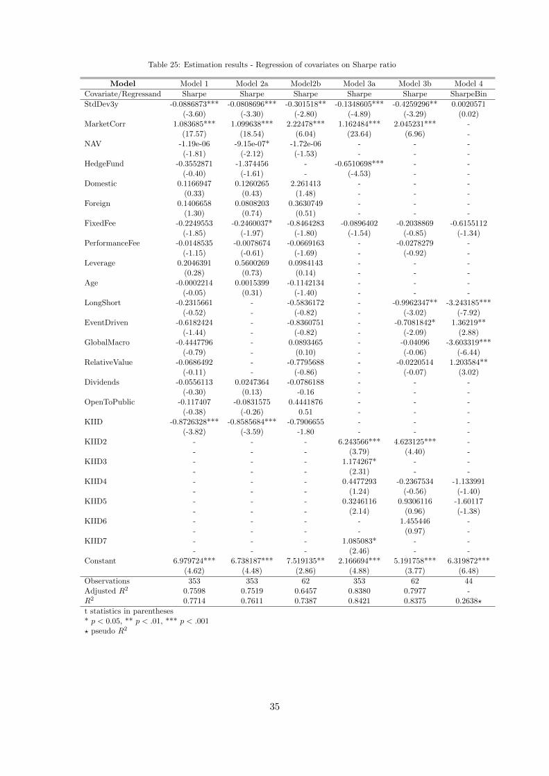
Table 25: Estimation results - Regression of covariates on Sharpe ratio

Model Model 1 Model 2a Model2b Model 3a Model 3b Model 4

Covariate/Regressand Sharpe Sharpe Sharpe Sharpe Sharpe SharpeBin

StdDev3y -0.0886873*** -0.0808696*** -0.301518** -0.1348605*** -0.4259296** 0.0020571(-3.60) (-3.30) (-2.80) (-4.89) (-3.29) (0.02)

MarketCorr 1.083685*** 1.099638*** 2.22478*** 1.162484*** 2.045231*** -(17.57) (18.54) (6.04) (23.64) (6.96) -

NAV -1.19e-06 -9.15e-07* -1.72e-06 - - -(-1.81) (-2.12) (-1.53) - - -

HedgeFund -0.3552871 -1.374456 - -0.6510698*** - -(-0.40) (-1.61) - (-4.53) - -

Domestic 0.1166947 0.1260265 2.261413 - - -(0.33) (0.43) (1.48) - - -

Foreign 0.1406658 0.0808203 0.3630749 - - -(1.30) (0.74) (0.51) - - -

FixedFee -0.2249553 -0.2460037* -0.8464283 -0.0896402 -0.2038869 -0.6155112(-1.85) (-1.97) (-1.80) (-1.54) (-0.85) (-1.34)

PerformanceFee -0.0148535 -0.0078674 -0.0669163 - -0.0278279 -(-1.15) (-0.61) (-1.69) - (-0.92) -

Leverage 0.2046391 0.5600269 0.0984143 - - -(0.28) (0.73) (0.14) - - -

Age -0.0002214 0.0015399 -0.1142134 - - -(-0.05) (0.31) (-1.40) - - -

LongShort -0.2315661 - -0.5836172 - -0.9962347** -3.243185***(-0.52) - (-0.82) - (-3.02) (-7.92)

EventDriven -0.6182424 - -0.8360751 - -0.7081842* 1.36219**(-1.44) - (-0.82) - (-2.09) (2.88)

GlobalMacro -0.4447796 - 0.0893465 - -0.04096 -3.603319***(-0.79) - (0.10) - (-0.06) (-6.44)

RelativeValue -0.0686492 - -0.7795688 - -0.0220514 1.203584**(-0.11) - (-0.86) - (-0.07) (3.02)

Dividends -0.0556113 0.0247364 -0.0786188 - - -(-0.30) (0.13) -0.16 - - -

OpenToPublic -0.117407 -0.0831575 0.4441876 - - -(-0.38) (-0.26) 0.51 - - -

KIID -0.8726328*** -0.8585684*** -0.7906655 - - -(-3.82) (-3.59) -1.80 - - -

KIID2 - - - 6.243566*** 4.623125*** -- - - (3.79) (4.40) -

KIID3 - - - 1.174267* - -- - - (2.31) - -

KIID4 - - - 0.4477293 -0.2367534 -1.133991- - - (1.24) (-0.56) (-1.40)

KIID5 - - - 0.3246116 0.9306116 -1.60117- - - (2.14) (0.96) (-1.38)

KIID6 - - - - 1.455446 -- - - - (0.97) -

KIID7 - - - 1.085083* - -- - - (2.46) - -

Constant 6.979724*** 6.738187*** 7.519135** 2.166694*** 5.191758*** 6.319872***(4.62) (4.48) (2.86) (4.88) (3.77) (6.48)

Observations 353 353 62 353 62 44Adjusted R2 0.7598 0.7519 0.6457 0.8380 0.7977 -R2 0.7714 0.7611 0.7387 0.8421 0.8375 0.2638?

t statistics in parentheses* p < 0.05, ** p < .01, *** p < .001? pseudo R2

35

7 Analysis

↪→ This section contains the analysis of the results, both the analysis of the regressionsresults in terms of numerics, as well as the econometric interpretation. We also discussthe results and connect the results to our theoretical framework, such as how our resultsgo along with the effective market hypothesis and different threats to internal validity ofthe model.

7.1 Econometric analysis

In the first model there was multicollinearity present between the HedgeFund covariateand the strategy covariates. This could be seen in the VIF table where the values of thementioned covariates were above the predetermined threshold, as well as in the correlationmatrix presented in Table 5. Thereby, we decided to do two sets of regression models.One which would include the HedgeFund covariate but not the strategy covariates andvice versa.

In the second model we used a stepwise regression method with the Bayesian InformationCriterion and the Akaike Information Criterion to remove non-explaining covariates. Dueto the fact that BIC penalizes non-explaining covariates harder, we conformed to BIC[15].Initially when including all covariates we received with R2 of 0.7714 and and adjusted-R2

of 0.7598. We also found there was a high multicollinearity between some covariates. Forinstance, we recognized that most hedge funds have a KIID value of either 5 or 6, soaccordingly, parts of the domain of KIID should be highly correlated with the hedge fundcovariate which is a potential cause for multicollinearity. This was solved by dividing theKIID covariate into six different binary covariates, which was possible due to the ratherlimited domain of the KIID covariate. All other covariates were below the predefinedthreshold.

By analyzing the results of the regressions for models 2a and 2b, we could see thatthe covariates domestic and foreign were severely penalized by the BIC as well as whensetting a tolerance p-value at 0.20. We found that this is due to that the covariates are notmutually exclusive. The funds can of course have both domestic and foreign investments.The covariate Age was also penalized by BIC, since removing the covariate generated alower BIC value. We found this results counter-intuitive, since we believed that olderfunds in general should have a higher Sharpe ratio than new funds.

In the third model, we removed the covariates suggested by the BIC and also as pre-viously mentioned divided our KIID covariate into six indicator covariates. We continuedwith two sets of regression models based on model 2. One where HedgeFund acted askey independent covariate, and one where the strategy covariates were the key depen-dent covariates. Since Model 3a has 3 covariates less than Model 3a, we compared theadjusted-R2. Model 3b has a slightly lower R2 value at 0.8375 compared to Model 3a,with a R2 of 0.8421. Since both versions of Model 3 are essential to explain whether hedgefunds provide a higher risk adjusted rate of return in terms of Sharpe ratio, both versionsare considered to be the final versions.

According to Model 3a, hedge funds generate a 0.6511 lower Sharpe ratio comparedto mutual funds. This estimate is statistically significant at a 0.1 % significance level.

36

However, since we used the risk-free rate of return as the benchmark index for both fundtypes, this results can be questioned. The two fund types have different objectives, thusthe results are not completely justified. However, due to lack of better ways to comparethe funds, we use the risk-free rate of return as benchmark for both fund types.

Our fourth model uses a probabilistic regression model. This was our primary idea,since our thesis question aims to answer a yes/no question and we make an extensive useof binary independent covariates. Therefore the probit regression model suits the datasetvery well. In Table 25 we can see that, all strategies are significant at the 1 % significancelevel. The probit estimates are negative for LongShort and GlobalMacro and positivefor EventDriven and RelativeV alue. When applying the probit model, we wanted toconclude whether the probability increases/decreases of a higher Sharpe ratio given a theusage of a certain strategy.

We have throughout the models non-normally distributed residuals. This is most likelyan effect of our limited number of observations. According to the central limit theoremhaving a large number of observations should make the residuals approximately normallydistributed. Model 3a and 3b display more centralized residuals than the previous models.The reason for the steeper residual curve is either the exclusion or inclusion of covariatesbetween the regression models, since these are the only aspects in which the models differ.

7.2 Threats to internal validity

When estimating regression models, there might be several threats to internal validitybut also external validity. The threats that we have recognized are sample selection bias,omitted variables bias as well as simultaneous causality bias.

7.2.1 Sample selection bias

In our case, the sampling scheme was to include the total number of mutual funds, as wellas all hedge funds in Sweden (including those not open to the public). The sample wasbased on the funds available on the 15th of March 2014. The data includes returns andSharpe ratio calculated for the preceding 3 years between 2011 and 2014. We estimatethe Sharpe ratio for mutual funds and hedge funds. The problem that might occur is thatthe sample only includes funds that has survived all three years without defaulting. Thesolution to this problem would be to change the sample population from the funds thatwere available in March 15th to the funds available in the beginning of of 2011, March 15th,including defunct funds. However, due to the fact that failed funds are excluded fromdata, finding data on failed funds is often very hard, there is no simple way of resolvingthis issue. By not including failed funds, both positive and negative biases are possible.There must be data available on whether hedge funds or mutual funds are more prone todefaulting. Only then can we discuss whether the bias is over- or underestimated.

7.2.2 Omitted variables bias

There are few cases where omitted variable bias does not occur. In our regression modelsOVB is a particular issue, due to the fact that hedge funds are generally more reluctantto give out information about holdings, market exposure etc. This makes it harder toestimate why certain hedge funds outperform others. Variables that would improve our

37

model would include a variable explaining market exposures, largest holdings, largestindustry exposure etc.

7.2.3 Simultaneous causality bias

Simultaneous causality bias occurs when there is reverse causal effect from the causal effectthat we are interested in. Such a bias might occur in our model through the correlationof the Sharpe ratio to the KIID covariates. Fund managers decide the classification of thefunds KIID. The classification is based on the volatility of the fund. Therefore one mightassume that the Sharpe ratio can have a causal effect on the KIID covariates. A solutionto this problem would be to use more sophisticated regression methods such as the useof an instrumental variable. However, we strongly believe that the correlation should notbe strong enough for a bias caused by simultaneous causality. The volatility of a fundchanges frequently whereas the KIID stays constant if not an active decision is made onthe core objective of the fund.

38

8 Adherence to Effective Market Hypothesis

↪→ In this section, we discuss how well hedge funds adhere to the effective market hypoth-esis. We compare and contrast our results to previous studies and finally conclude onwhether Swedish hedge funds contradict the EMH.

8.1 Empirical findings

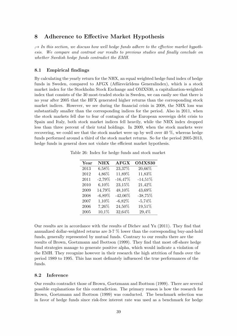
By calculating the yearly return for the NHX, an equal weighted hedge fund index of hedgefunds in Sweden, compared to AFGX (Affarsvarldens Generalindex), which is a stockmarket index for the Stockholm Stock Exchange and OMXS30, a capitalization-weightedindex that consists of the 30 most-traded stocks in Sweden, we can easily see that there isno year after 2005 that the HFX generated higher returns than the corresponding stockmarket indices. However, we see during the financial crisis in 2008, the NHX loss wassubstantially smaller than the corresponding indices for the period. Also in 2011, whenthe stock markets fell due to fear of contagion of the European sovereign debt crisis toSpain and Italy, both stock market indices fell heavily, while the NHX index droppedless than three percent of their total holdings. In 2009, when the stock markets wererecovering, we could see that the stock market were up by well over 40 %, whereas hedgefunds performed around a third of the stock market returns. So for the period 2005-2013,hedge funds in general does not violate the efficient market hypothesis.

Table 26: Index for hedge funds and stock market

Year NHX AFGX OMXS30

2013 6,58% 23,37% 20,66%2012 4,86% 11,89% 11,83%2011 -2,79% -16,47% -14,51%2010 6,10% 23,15% 21,42%2009 14,79% 48,10% 43,69%2008 -6,89% -42,06% -38,75%2007 1,10% -6,82% -5,74%2006 7,26% 24,50% 19,51%2005 10,1% 32,64% 29,4%

Our results are in accordance with the results of Dichev and Yu (2011). They find thatannualized dollar-weighted returns are 3-7 % lower than the corresponding buy-and-holdfunds, generally represented by mutual funds. Contrary to our results there are theresults of Brown, Goetzmann and Ibottson (1999). They find that most off-shore hedgefund strategies manage to generate positive alpha, which would indicate a violation ofthe EMH. They recognize however in their research the high attrition of funds over theperiod 1989 to 1995. This has most definately influenced the true performances of thefunds.

8.2 Inference

Our results contradict those of Brown, Goetzmann and Ibottson (1999). There are severalpossible explanations for this contradiction. The primary reason is how the research forBrown, Goetzmann and Ibottson (1999) was conducted. The benchmark selection wasin favor of hedge funds since risk-free interest rate was used as a benchmark for hedge

39

funds and indices for the mutual funds. Since hedge funds can buy, for example, stocksconnected to any index, hedge funds can in theory have perfect correlation to an index.This would mean that hedge funds performs as a mutual fund but its performance isjudged in relation to the, often significantly lower, risk-free interest rate.

Another reason for this contradiction could be the difference in time periods. Our resultsare based on data over the period 2011-2014, where the severe financial crisis has hada longlasting impact on the financial markets, whereas Brown, Goetzmann and Ibottson(1999) studies off-shore hedge funds based on data over the period 1989-1995. Accordingto our results, we do not find that hedge funds violate the efficient market hypothesis,i.e. we do not find any evidence that hedge funds consistently outperform the market.However, this is not the objective for hedge funds either.

Hedge funds have the objective to generate absolute returns, and perhaps more im-portantly, achieve stable returns to a reasonable risk level, while having a low marketcorrelation. Also, to say that hedge funds in general do not violate the effective markethypothesis is not the same as saying that are not some hedge funds manage to continuouslyoutperform the market, which can be read more in detail in Fung and Hsieh (2011).

40

9 Preferred investment strategy

↪→ In this section, we discuss the preferred investment strategy from a hedge fund man-agers view. We determine the investment strategy most used and discuss underlying rea-sons based on conducted interviews.

In order to answer the question whether there is an investment strategy that is usedmore frequently than others, we conducted two interviews with managers at twodifferent hedge funds, Christian Carping at DNB and Ulf Berg and Krister Sjoblom ateTurn Fonder. Carping is the manager of a multi-strategy hedge fund and therefore hehas an overbridging view of strategies. From his point of view, aside from being stableand profitable, hedge funds should also be market neutral. For him, as a manager of amulti-strategy fund, the correlation between both hedge fund strategies as well asbetween specific funds is important since the purpose of using a multi-strategy is toremove some of the risk by diversifying. Berg and Sjoblom run eTurn, which is acompany with several hedge funds. The funds all use the same strategy, an event drivenstrategy based on quantitative computer models. Since they only use one strategy theyhave a less clasping view of hedge fund strategies and more of an in-depth view of eventdriven strategies. Since they do not have an objective view of strategies, the interviewdid not include questions about their preferred strategy and what they value in astrategy.

9.1 Inferences from interviews

During both interviews it was stated that hedge funds are fairly uncommon in Swedenand Carping states that it is hard to make a diversified multi-strategy fund in Sweden,which would indicate that there is an uneven distribution of hedge fund strategies. Ourdata suggests that long/short strategies are the most common and this is strengthened bythe interview with Carping, in which he stated that Sweden is a “stock country” where itis relatively common for individuals to own stocks. This has, according to him, translatedinto a relatively large amount of mutual funds and it could also help explain the largeamount of hedge funds using long/short strategies we have seen in our data.

Another potential cause for the relatively large amount of long/short hedge funds is that,according to Carping, small thresholds present for starting a stock-based (long/short)hedge fund. Our intution is also strengthened by Berg and Sjoblom who said that theirstrategy is fairly rare in Sweden. This is quite strange since Berg and Sjoblom statesthat Sweden and the Nordic area showcase properties suitable for event driven strategies.Though according to both interviews, event driven strategies, has had a hard time per-forming well since the financial crisis of 2008 when many of the event-driven went reallywell. This is, according to Carping (who decided not to invest in event driven strategies),an effect of the central banks decisions to “terminate” events and pushing down interestrates. Below we have the representation of hedge fund strategies in our dataset. Basedon this the most common strategy is long/short which corresponds to 50.0 % of the hedgefund strategies. Which would indicate that long/short is the preferred strategy of hedgefund managers in Sweden.6

6http://fondbolagen.se/sv/Studier/Studier/Fakta-8-av-10-svenskar-sparar-i-fonder/

41

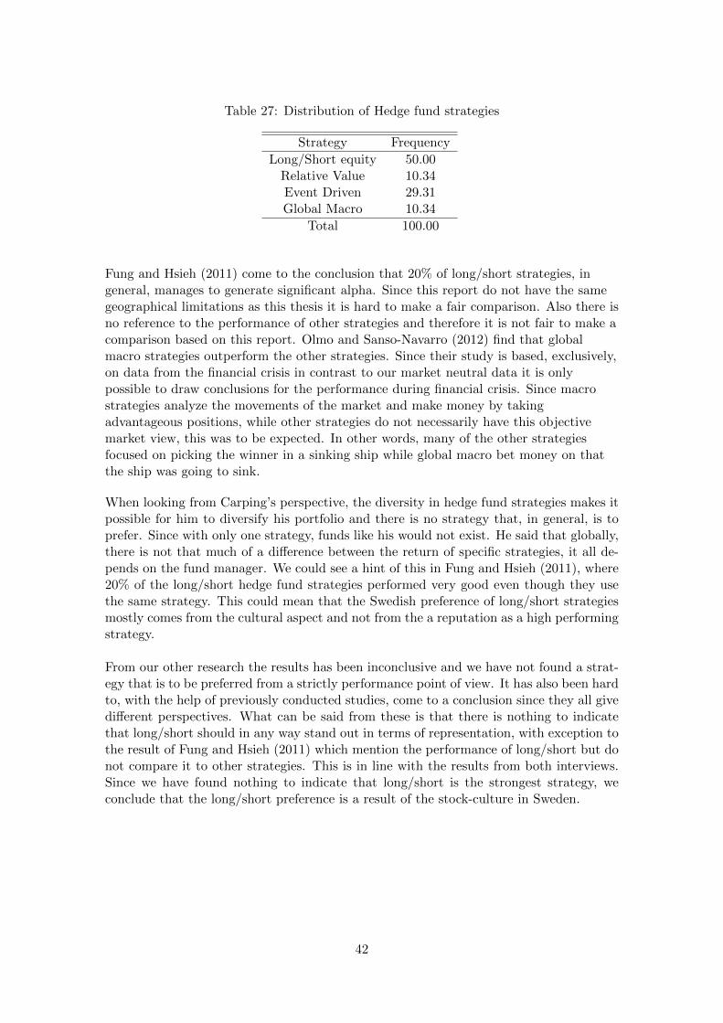
Table 27: Distribution of Hedge fund strategies

Strategy Frequency

Long/Short equity 50.00Relative Value 10.34Event Driven 29.31Global Macro 10.34

Total 100.00

Fung and Hsieh (2011) come to the conclusion that 20% of long/short strategies, ingeneral, manages to generate significant alpha. Since this report do not have the samegeographical limitations as this thesis it is hard to make a fair comparison. Also there isno reference to the performance of other strategies and therefore it is not fair to make acomparison based on this report. Olmo and Sanso-Navarro (2012) find that globalmacro strategies outperform the other strategies. Since their study is based, exclusively,on data from the financial crisis in contrast to our market neutral data it is onlypossible to draw conclusions for the performance during financial crisis. Since macrostrategies analyze the movements of the market and make money by takingadvantageous positions, while other strategies do not necessarily have this objectivemarket view, this was to be expected. In other words, many of the other strategiesfocused on picking the winner in a sinking ship while global macro bet money on thatthe ship was going to sink.

When looking from Carping’s perspective, the diversity in hedge fund strategies makes itpossible for him to diversify his portfolio and there is no strategy that, in general, is toprefer. Since with only one strategy, funds like his would not exist. He said that globally,there is not that much of a difference between the return of specific strategies, it all de-pends on the fund manager. We could see a hint of this in Fung and Hsieh (2011), where20% of the long/short hedge fund strategies performed very good even though they usethe same strategy. This could mean that the Swedish preference of long/short strategiesmostly comes from the cultural aspect and not from the a reputation as a high performingstrategy.

From our other research the results has been inconclusive and we have not found a strat-egy that is to be preferred from a strictly performance point of view. It has also been hardto, with the help of previously conducted studies, come to a conclusion since they all givedifferent perspectives. What can be said from these is that there is nothing to indicatethat long/short should in any way stand out in terms of representation, with exception tothe result of Fung and Hsieh (2011) which mention the performance of long/short but donot compare it to other strategies. This is in line with the results from both interviews.Since we have found nothing to indicate that long/short is the strongest strategy, weconclude that the long/short preference is a result of the stock-culture in Sweden.

42

10 Conclusions

By the use of a multiple linear regression model it has been shown that Swedish hedgefunds do not generate as high risk-adjusted returns as Swedish mutual funds, when usingthe same benchmark. In regards to best performing hedge fund investment strategyin Sweden, the results have been inconclusive. Our results show that the long/shortand global macro strategies tend to have a lower Sharpe ratio, and event driven andrelative value strategies have a higher Sharpe ratio. We believe however that due tothe low number of observations, one cannot fully conclude which strategy is the highestperforming. Though data show that long/short strategies are preferred by Swedish hedgefund managers. The reason for this seems to be the stock culture in Sweden according tointerviews with hedge fund managers. Also, by studying literature and index performancesit has been shown that hedge funds do not violate the effective market hypothesis.

11 Future research

Hedge funds have been around for 50 years and have become more significant in playingthe role of allocating capital in the financial markets in order to make it more efficient.Hedge funds have also become more important on the Swedish market, which can easilybe seen, because of the growth of hedge funds in Sweden have on average been largerthan worldwide. This leads to that in future research, more hedge funds can be includedin order to get a greater reliability, but also validity. In order to successfully examinedifferent investment strategies in contrast to market indices, the future research shouldbe based more on monthly returns rather than yearly. In order to understand Swedishhedge funds more in depth, they should be compared on the global market for hedgefunds, for instance with hedge funds based in New York and London, where hedge fundsare more established. Also the traditional risk-measures for funds cannot be applied tohedge funds as well as to mutual funds. We also think that more research is neededtowards finding appropriate methods for comparing hedge funds to mutual funds.

43

References

[1] Berk, J.,DeMarzo, P., 2013, Corporate Finance 3rd Edition, Prentice Hall.

[2] Jensen, M. C., 1967, The Performance Of Mutual Funds In The Period 1945-1964,The Journal of Finance, Volyme 23, Issue 2, Pages 389-416.

[3] Anderlind, P., Eidolf, E., Holm, M., Sommerlau, P., 2003, Hedgefonder, First edi-tion, Academia Adacta, Lund.

[4] Connor, G., Woo M., 2004, An Introduction to Hedge Funds, Introductory Guide,The London School of Economics and Political Science.

[5] Ackermann, C., Richard McEnally, R., Ravenscraft, D., 1999, The Performance ofHedge Funds: Risk, Return, and Incentives, The Journal of Finance, Volume 54,Issue 3, Pages 833–874.

[6] Liang, B., 1998, On the Performance of Hedge Funds, University of Massachusettsat Amherst, Working Paper Series, Social Science Research Network.

[7] Dicheva, I. D., Yu, G., 2011, Higher risk, lower returns: What hedge fund investorsreally earn, Journal of Financial Economics Volume 100, Issue 2, Pages 248–263.

[8] Capocci, D., Hubner, G., 2004, Analysis of hedge fund performance, Journal ofEmpirical Finance, Volume 11, Issue 1, Pages 55–89.

[9] Brown, S., Goetzmann, W., Ibbotson, R., 1999, Offshore Hedge Funds: Survival andPerformance, 1989-95,The Journal of Business, Volume 72, Issue 1, Pages 91-117.

[10] Olmo, J., Sanso-Navarro, M., 2012, Forecasting the performance of hedge fund stylesJournal of Banking & Finance, Volume 36, Issue 8, Pages 2351–2365.

[11] Fung, W.,Hsieh, D. A., 2011, The risk in hedge fund strategies: Theory and evidencefrom long/short equity hedge funds Journal of Empirical Finance, Volume 18, Issue4, Pages 547–569.

[12] Lang, H., 2013, Topics on Applied Mathematical Statistics, KTH Teknikvetenskap.

[13] Stock, J. H., Watson, M. M., 2012, Introduction to Econometrics, third edition,Global Edition, Pearson Education Limited.

[14] Kennedy, P., 2012, A Guide to Econometrics, 5th edition, Blackwell Publishing.

[15] Dziak, J. J., Coffman, D. L.,Lanza, S. T., Li, R., 2012, Sensitivity and specificity ofinformation criteria, The Pennsylvania State University.

44

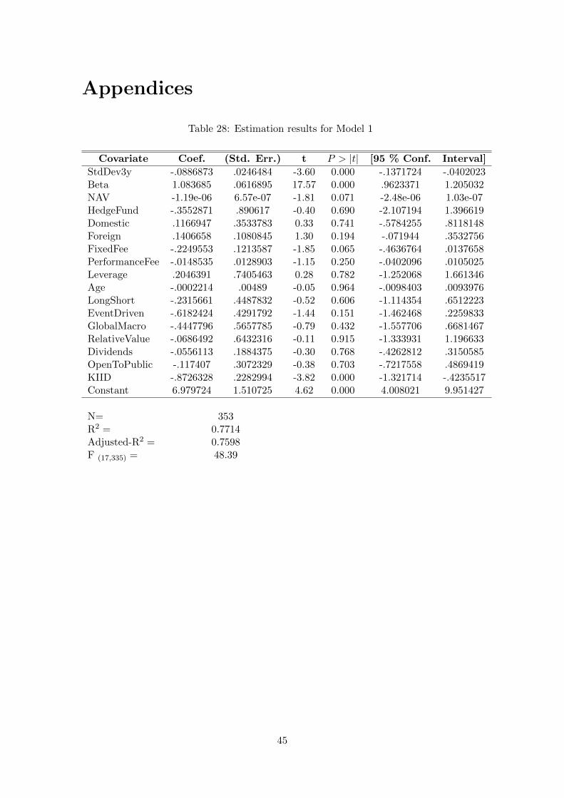
Appendices

Table 28: Estimation results for Model 1

Covariate Coef. (Std. Err.) t P > |t| [95 % Conf. Interval]

StdDev3y -.0886873 .0246484 -3.60 0.000 -.1371724 -.0402023Beta 1.083685 .0616895 17.57 0.000 .9623371 1.205032NAV -1.19e-06 6.57e-07 -1.81 0.071 -2.48e-06 1.03e-07HedgeFund -.3552871 .890617 -0.40 0.690 -2.107194 1.396619Domestic .1166947 .3533783 0.33 0.741 -.5784255 .8118148Foreign .1406658 .1080845 1.30 0.194 -.071944 .3532756FixedFee -.2249553 .1213587 -1.85 0.065 -.4636764 .0137658PerformanceFee -.0148535 .0128903 -1.15 0.250 -.0402096 .0105025Leverage .2046391 .7405463 0.28 0.782 -1.252068 1.661346Age -.0002214 .00489 -0.05 0.964 -.0098403 .0093976LongShort -.2315661 .4487832 -0.52 0.606 -1.114354 .6512223EventDriven -.6182424 .4291792 -1.44 0.151 -1.462468 .2259833GlobalMacro -.4447796 .5657785 -0.79 0.432 -1.557706 .6681467RelativeValue -.0686492 .6432316 -0.11 0.915 -1.333931 1.196633Dividends -.0556113 .1884375 -0.30 0.768 -.4262812 .3150585OpenToPublic -.117407 .3072329 -0.38 0.703 -.7217558 .4869419KIID -.8726328 .2282994 -3.82 0.000 -1.321714 -.4235517Constant 6.979724 1.510725 4.62 0.000 4.008021 9.951427

N= 353R2 = 0.7714Adjusted-R2 = 0.7598F (17,335) = 48.39

45

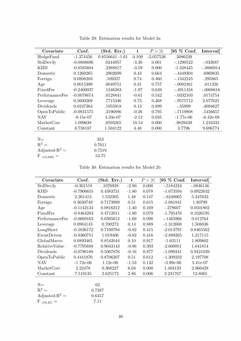
Table 29: Estimation results for Model 2a

Covariate Coef. (Std. Err.) t P > |t| [95 % Conf. Interval]

HedgeFund -1.374456 0.8556641 -1.61 0.109 -3.057536 .3086239StdDev3y -0.0808696 .0244957 -3.30 0.001 -.1290522 -.032687KIID -0.8585684 .2388817 -3.59 0.000 -1.328445 -.3886914Domestic 0.1260265 .2902699 0.43 0.664 -.4449304 .6969835Foreign 0.0808203 .109327 0.74 0.460 -.1342245 .295865Age 0.0015399 .0049751 0.31 0.757 -.0082461 .011326FixedFee -0.2460037 .1246283 -1.97 0.049 -.4911458 -.0008616PerformanceFee -0.0078674 .0128841 -0.61 0.542 -.0332103 .0174754Leverage 0.5600269 .7715346 0.73 0.468 -.9575712 2.077625Dividends 0.0247364 .1955918 0.13 0.899 -.35999 .4094627OpenToPublic -0.0831575 .3196886 -0.26 0.795 -.7119808 .5456657NAV -9.15e-07 4.33e-07 -2.12 0.035 -1.77e-06 -6.42e-08MarketCorr 1.099638 .0593265 18.54 0.000 .9829439 1.216333Constant 6.738187 1.504122 4.48 0.000 3.7796 9.696774

N= 353R2 = 0.7611Adjusted-R2 = 0.7519F (13,339) = 53.75

Table 30: Estimation results for Model 2b

Covariate Coef. (Std. Err.) t P > |t| [95 % Conf. Interval]

StdDev3y -0.301518 .1076928 -2.80 0.008 -.5184224 -.0846136KIID -0.7906655 0.4383731 -1.80 0.078 -1.673594 0.0922632Domestic 2.261413 1.532305 1.48 0.147 -.8248065 5.347633Foreign 0.3630749 0.7173989 0.51 0.615 -1.081841 1.80799Age -0.1142134 0.0816212 -1.40 0.169 -.278607 0.0501802FixedFee -0.8464283 0.4712011 -1.80 0.079 -1.795476 0.1026195PerformanceFee -0.0669163 0.0395612 -1.69 0.098 -.1465966 0.012764Leverage 0.0984143 0.700273 0.14 0.889 -1.312008 1.508836LongShort -0.5836172 0.7100794 -0.82 0.415 -2.013791 0.8465562EventDriven -0.8360751 1.019406 -0.82 0.416 -2.889265 1.217115GlobalMacro 0.0893465 0.8542044 0.10 0.917 -1.63111 1.809802RelativeValue -0.7795688 0.9043143 -0.86 0.393 -2.600951 1.041814Dividends -0.0786188 0.5067876 -0.16 0.877 -1.099341 0.9421039OpenToPublic 0.4441876 0.8706207 0.51 0.612 -1.309332 2.197708NAV -1.72e-06 1.12e-06 -1.53 0.132 -3.99e-06 5.41e-07MarketCorr 2.22478 0.368227 6.04 0.000 1.483133 2.966428Constant 7.519135 2.625172 2.86 0.006 2.231767 12.8065

N= 62R2 = 0.7387Adjusted-R2 = 0.6457F (16,45) = 7.11

46

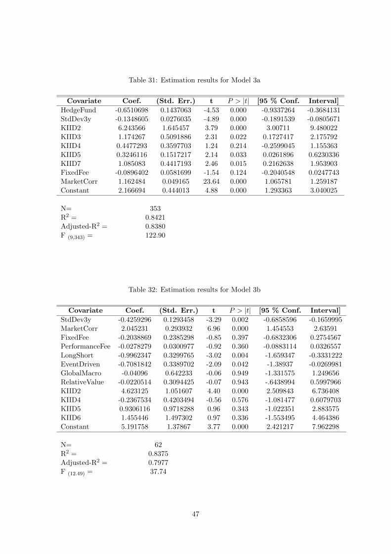
Table 31: Estimation results for Model 3a

Covariate Coef. (Std. Err.) t P > |t| [95 % Conf. Interval]

HedgeFund -0.6510698 0.1437063 -4.53 0.000 -0.9337264 -0.3684131StdDev3y -0.1348605 0.0276035 -4.89 0.000 -0.1891539 -0.0805671KIID2 6.243566 1.645457 3.79 0.000 3.00711 9.480022KIID3 1.174267 0.5091886 2.31 0.022 0.1727417 2.175792KIID4 0.4477293 0.3597703 1.24 0.214 -0.2599045 1.155363KIID5 0.3246116 0.1517217 2.14 0.033 0.0261896 0.6230336KIID7 1.085083 0.4417193 2.46 0.015 0.2162638 1.953903FixedFee -0.0896402 0.0581699 -1.54 0.124 -0.2040548 0.0247743MarketCorr 1.162484 0.049165 23.64 0.000 1.065781 1.259187Constant 2.166694 0.444013 4.88 0.000 1.293363 3.040025

N= 353R2 = 0.8421Adjusted-R2 = 0.8380F (9,343) = 122.90

Table 32: Estimation results for Model 3b

Covariate Coef. (Std. Err.) t P > |t| [95 % Conf. Interval]

StdDev3y -0.4259296 0.1293458 -3.29 0.002 -0.6858596 -0.1659995MarketCorr 2.045231 0.293932 6.96 0.000 1.454553 2.63591FixedFee -0.2038869 0.2385298 -0.85 0.397 -0.6832306 0.2754567PerformanceFee -0.0278279 0.0300977 -0.92 0.360 -0.0883114 0.0326557LongShort -0.9962347 0.3299765 -3.02 0.004 -1.659347 -0.3331222EventDriven -0.7081842 0.3389702 -2.09 0.042 -1.38937 -0.0269981GlobalMacro -0.04096 0.642233 -0.06 0.949 -1.331575 1.249656RelativeValue -0.0220514 0.3094425 -0.07 0.943 -.6438994 0.5997966KIID2 4.623125 1.051607 4.40 0.000 2.509843 6.736408KIID4 -0.2367534 0.4203494 -0.56 0.576 -1.081477 0.6079703KIID5 0.9306116 0.9718288 0.96 0.343 -1.022351 2.883575KIID6 1.455446 1.497302 0.97 0.336 -1.553495 4.464386Constant 5.191758 1.37867 3.77 0.000 2.421217 7.962298

N= 62R2 = 0.8375Adjusted-R2 = 0.7977F (12.49) = 37.74

47

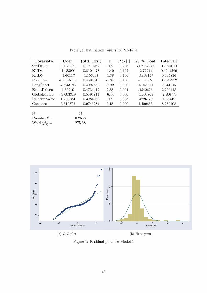
Table 33: Estimation results for Model 4

Covariate Coef. (Std. Err.) z P > |z| [95 % Conf. Interval]

StdDev3y 0.0020571 0.1210962 0.02 0.986 -0.2352872 0.2394013KIID4 -1.133991 0.8104478 -1.40 0.162 -2.72244 0.4544569KIID5 -1.60117 1.156647 -1.38 0.166 -3.868157 0.665816FixedFee -0.6155112 0.4594515 -1.34 0.180 -1.51602 0.2849972LongShort -3.243185 0.4092552 -7.92 0.000 -4.045311 -2.44106EventDriven 1.36219 0.4734412 2.88 0.004 .4342626 2.290118GlobalMacro -3.603319 0.5594714 -6.44 0.000 -4.699863 -2.506775RelativeValue 1.203584 0.3984289 3.02 0.003 .4226779 1.98449Constant 6.319872 0.9746284 6.48 0.000 4.409635 8.230108

N= 44Pseudo R2 = 0.2638Wald χ2

(8) = 275.68

−2

02

46

Resid

uals

−4 −2 0 2 4

Inverse Normal

(a) Q-Q plot

050

100

150

Fre

quency

−2 0 2 4 6

Residuals

(b) Histogram

Figure 1: Residual plots for Model 1

48

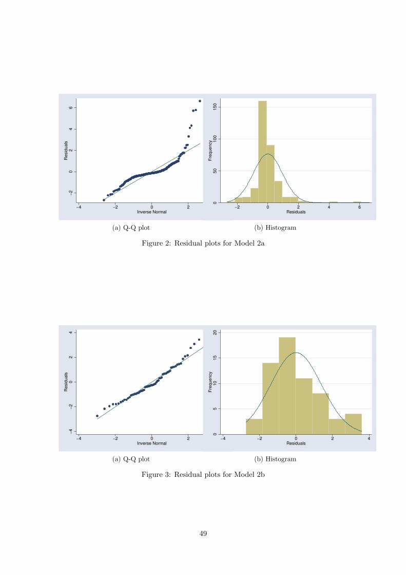
−2

02

46

Resid

uals

−4 −2 0 2 4

Inverse Normal

(a) Q-Q plot

050

100

150

Fre

quency

−2 0 2 4 6

Residuals

(b) Histogram

Figure 2: Residual plots for Model 2a

−4

−2

02

4

Resid

uals

−4 −2 0 2 4

Inverse Normal

(a) Q-Q plot

05

10

15

20

Fre

quency

−4 −2 0 2 4

Residuals

(b) Histogram

Figure 3: Residual plots for Model 2b

49

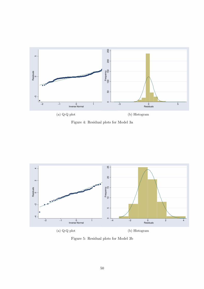
−5

05

Resid

uals

−2 −1 0 1 2

Inverse Normal

(a) Q-Q plot

050

100

150

200

250

Fre

quency

−5 0 5

Residuals

(b) Histogram

Figure 4: Residual plots for Model 3a

−4

−2

02

4

Resid

uals

−2 −1 0 1 2

Inverse Normal

(a) Q-Q plot

05

10

15

20

25

Fre

quency

−4 −2 0 2 4

Residuals

(b) Histogram

Figure 5: Residual plots for Model 3b

50

TRITA -MAT-K 2014:04

ISRN -KTH/MAT/K--14/04-SE

www.kth.se