1 Do Food Scares Explain Supplier Concentration? An Analysis of EU Agri-food Imports § July 2009 Mélise Jaud * Olivier Cadot + Akiko Suwa Eisenmann+ Abstract This paper documents a decreasing trend in the geographical concentration of EU agro- food imports. Decomposing the concentration indices into intensive and extensive margins components, we find that the decrease in overall concentration indices results from two diverging trends: the pattern of trade diversifies at the extensive margin (EU countries have been sourcing their agri-food products from a wider range of suppliers), while geographical concentration increases at the intensive-margin (EU countries have concentrated their imports on a few major suppliers). This leads to an increasing inequality in market shares between a small group of large suppliers and a majority of small suppliers. We then move on to exploit a database of food alerts at the EU border that had never been exploited before. After coding it into HS8 categories, we regress the incidence of food alerts by product on determinants including exporter dummies as well as HS8 product dummies. Coefficients on product dummies provide unbiased estimates of the intrinsic vulnerability of exported products to food alerts, as measured at the EU border. We incorporate the product risk coefficient as an explanatory variable in a regression of geographical concentration and show that concentration is higher for risky products. Keywords: European Union, import concentration, sanitary risk, food, agricultural trade JEL classification codes: F1, O13, Q17, Q18 § Without implicating them, we thank participants to a seminar at the Paris School of Economics, in particular Anne-Célia Disdier and Lionel Fontagné, for helpful comments on a earlier version. * Paris School of Economics + University of Lausanne, CEPR, CERDI and CEPREMAP. + INRA, LEA , Paris School of Economics.

Welcome message from author
This document is posted to help you gain knowledge. Please leave a comment to let me know what you think about it! Share it to your friends and learn new things together.
Transcript

1
Do Food Scares Explain Supplier Concentration?
An Analysis of EU Agri-food Imports§
July 2009
Mélise Jaud∗
Olivier Cadot+
Akiko Suwa Eisenmann+
Abstract
This paper documents a decreasing trend in the geographical concentration of EU agro-food imports. Decomposing the concentration indices into intensive and extensive margins components, we find that the decrease in overall concentration indices results from two diverging trends: the pattern of trade diversifies at the extensive margin (EU countries have been sourcing their agri-food products from a wider range of suppliers), while geographical concentration increases at the intensive-margin (EU countries have concentrated their imports on a few major suppliers). This leads to an increasing inequality in market shares between a small group of large suppliers and a majority of small suppliers. We then move on to exploit a database of food alerts at the EU border that had never been exploited before. After coding it into HS8 categories, we regress the incidence of food alerts by product on determinants including exporter dummies as well as HS8 product dummies. Coefficients on product dummies provide unbiased estimates of the intrinsic vulnerability of exported products to food alerts, as measured at the EU border. We incorporate the product risk coefficient as an explanatory variable in a regression of geographical concentration and show that concentration is higher for risky products. Keywords: European Union, import concentration, sanitary risk, food, agricultural trade
JEL classification codes: F1, O13, Q17, Q18
§ Without implicating them, we thank participants to a seminar at the Paris School of Economics, in particular Anne-Célia Disdier and Lionel Fontagné, for helpful comments on a earlier version. ∗ Paris School of Economics + University of Lausanne, CEPR, CERDI and CEPREMAP. + INRA, LEA , Paris School of Economics.

2
1. Introduction
After a series of highly publicized food scares (bovine spongiform
encephalopathy or dioxin-contaminated chickens to name but two), public-
health concerns have started to loom large in the buying policies of EU foodstuff
distributors. These concerns have the potential to affect the evolution of EU
foodstuff imports, and therefore the access that developing countries—in
particular the poorest ones, who find it most difficult to comply with stringent
sanitary standards—enjoy on EU markets (Maskus et al. 2005). This is
particularly important for products like fruit & vegetables or fisheries products,
which represent a growing share of EU food imports and are also of particular
concern to the least developed countries ( Jaffee et al 2004, World Bank 2005).
The impact of sanitary concerns on industrial-country foodstuff imports has
been studied extensively, essentially by sticking standards as explanatory
variables in gravity equations (see e.g. Moenius 1999, Maskus et al. 2000,
Otzuki and Wilson 2001, Sheperd and Wilson 2007). Estimation of such models
has highlighted the trade restrictiveness of such standards (Fontagné et al 2005,
Disdier, Fontagné et al. 2008).
We differentiate ourselves from the existing literature in two ways. First, we
shift focus from gravity modelling to an analysis of the geographical
concentration of EU foodstuff imports, using conventional and non-
conventional concentration measures (similar approaches can be found in Imbs
and Wacziarg 2003 for production or in Cadot, Carrère and Strauss-Kahn 2007,
and Dutt, Mihov and van Zandt 2008 for exports). We propose a decomposition
of Theil’s entropy index between active and potential suppliers with the
property that variations in the index’s within- and between-group components
map directly into intensive- and extensive-margin variations. We also propose a
variant of Hummels and Klenow’s intensive and extensive margins (which they
developed for the analysis of the product-wise concentration of exports) adapted
to imports and to geographical concentration.
Our product-level analysis shows that, over the last two decades, EU foodstuff
imports have concentrated, geographically, at the intensive margin. That is, on
average, at the product-line (HS8) level, the market shares of active suppliers
have diverged. However, we also observe a trend toward diversification at the
extensive margin. That is, again at the product-line level, the EU sources its
foodstuffs from an increasing number of exporting countries. These two

3
observations appear, at first sight, to be contradictory. Using our adaptation of
Hummels and Klenow’s intensive and extensive margins, we show that the
number of suppliers used by the EU is indeed increasing, but by addition of a
fringe of small-volume exporters. Thus, EU foodstuff imports gradually evolve
toward a two-tier distribution with a small number of increasingly dominant
suppliers and a growing fringe of marginal ones.
Second, we shift focus from standards, which affect trade flows ex-ante, to
alerts, which affect them ex-post. What we call here a “food alert” is the
notification of a contaminated foodstuff shipment at the external border of an
EU member state. Food alerts have the power to alter buyer perceptions of the
quality of particular suppliers. They could either lead to reinforced
concentration if buyers react by eliminating fringe suppliers perceived as
dubious by analogy with the culprit, or, alternatively, to the destruction of
dominant positions if they affect dominant suppliers. This is what we explore,
using an original database constructed from the European Commission’s Rapid
Alert System for Food and Feed (RASSF) database. Technically, the EU
Commission classifies contaminated-shipment notifications into two types:
“informations”, which lead to the destruction or re-routing of the concerned
shipment, or “alerts” stricto sensu which lead to the destruction or re-routing of
all shipments from the same exporting country at all EU borders. Since 2001, all
informations (about 19’000 of them) have been recorded in a detailed database,
which has never been used. We coded that database into HS8 product categories
to make it compatible with trade data, generating a population of events each
defined at the (product × exporter × year) level.
The RASFF database shows substantial heterogeneity in the incidence of food
alerts across exporting countries. This implies that a raw count of alerts by
product cannot give a correct proxy for product-specific sanitary risk. For
instance, a product imported overwhelmingly from a country with weak quality
standards would appear as risky even though other exporters might have
managed to make the product safe. In addition, the incidence of notifications is
likely to be correlated with the frequency of controls. Those controls may not be
purely random: they may reflect a particular exporter’s past performance or
hidden protectionism. Thus, regressing concentration indices on the frequency
of notifications at the product level would say nothing without controlling for
other factors.

4
In order to get an unbiased estimate of product-specific sanitary risk, we rely on
a two-step procedure. In the first step, we estimate product-specific sanitary risk
with a regression of the count of food alerts at EU borders over the sample
period, using an original database described in the next section. The unit of
observation is a product × exporter pair where alerts are summed over all years in the sample period. The regressors are exporting-country characteristics and
product dummies. Estimated coefficients on those product dummies give us an
estimated measure of product risk. In a second step, we regress the evolution of
geographical concentration indices on our measure of product risk and time
dummies.
Overall, we find that except for fisheries products no chapter stands out as
having particularly high risk levels. Incorporating our constructed measure of
product risk as an explanatory variable in a regression of geographical
concentration confirms that product riskiness affects sourcing concentration.
Product riskiness leads to reinforced concentration at the intensive margin and
reinforced diversification at the extensive margin. Thus, the distribution of EU
suppliers for riskiest agrofood imports is converging towards a pattern of
increasingly dominant suppliers with a growing fringe of small-scale ones.
The paper proceeds as follows. The next Section analyses the trend in the
geographical concentration of EU agro-food imports both at the intensive and
extensive margin. We then outline the EU "Food Alerts" Database in Section 3,
contrast it with previous data collection efforts, and present some descriptive
results. Section 3 then explores the impact of product riskiness on the patterns
of concentration. Section 4 concludes.
5
2. Agri-food supplier concentration
2.1 Overall diversification
2.1.1 The data
We use EUROSTAT agri-food import data covering EU-12 member states1
(France, Belgium-Luxembourg, the Netherlands, Germany, Italy, Ireland,
United Kingdom, Denmark, Greece, Portugal and Spain) between 1988 and
2005 at the HS8 level (the highest level of disaggregation available, as Eurostat
does not make 10-digit data available to researchers). Agri-food products,
excluding beverages and animal feed, are in chapters 1 to 21 of the HS system,
which represent 3’073 potential export lines. With 146 partner countries
(exporters) including 122 developing countries, we have a four-dimensional
panel where the unit of observation is a product imported by an EU member
state from an extra-EU partner in a given year.2 For some calculations, however,
we aggregate import data across EU member countries, reducing the panel’s
dimension to three (product × exporter × year).
At the HS8 level, reclassifications are frequent. Five types of reclassification can
be distinguished: (i) creation of a new code corresponding to a new product; (ii)
creation of several new codes by splitting a former one; (iii) creation of a new
code by merging several former ones; (iv) creation of new codes resulting from a
change in the coding system (HS harmonizations in 1988, 1996 and 2002); and
finally (v) termination of old codes. Of the 3’073 HS8 codes available in our
dataset, only 37.7% are unaffected by reclassification between 1988 and 2005.
Of the remainder (62.3%), 1.6% are new products (type i), and 0.7% are
terminated codes (type v). This leaves 60% of reclassifications of “continued”
1 We use this restrictive definition for consistency of time series, as EUROSTAT does not provide data on member states before their accession.
2 We drop intra-EU trade on the ground of the mutual recognition of standard. The principle ensures that a product lawfully produced in one Member State is acceptable without adaptation in another Member State, provided that both states pursue the same general objectives in health

6
products. Among those, half (30%) are type-ii reclassifications (splittings) and
half are type-iv (system changes).
In order to reduce the inconsistencies introduced by type-iii and type-iv
reclassifications to a minimum, we used EUROSTAT’s documentation to re-
reclassify new codes into initial ones; in case (iii), where a new code was made
out of several old ones, we used the first parent’s code in the HS order. This
gives us a consistent database using the initial nomenclature throughout the
sample period.
2.1.2 Trade relationships at the product level
Table 1 shows the evolution of the structure of EU agri-food imports between
1988 and 2005. The share of developing countries, already dominant at 68% at
the start of the sample period (1988), grew even more dominant, reaching 77%
in 2005. Interestingly, this rise is not attributable to a rise in imports of
traditional tropical products (coffee, cocoa, sugar, etc.) which, as a share of
imports from developing countries, shrank from 25.2% to 15.7% over the sample
period. Rather, it is due to a spectacular rise in imports of horticulture and
fisheries products, whose share rose from 21.2% to 30% of EU agri-food imports
from developing countries. This is remarkable given that fisheries and
horticulture products are, in general, fairly sensitive to sanitary and phyto-
sanitary issues, and the ability to meet stringent SPS standards is, in general,
correlated with exporter income.

7
Table 1 Evolution of EU imports structure, between 1988 and 2005
1988 2005 1988 2005 1988 2005
Traditional tropical products
Coffee, tea, mate and spices 16.6% 7.7% 0.1% 0.1% 16.7% 7.8%
Lacs; gums, resins 0.5% 0.7% 0.1% 0.2% 0.7% 0.9%
Sugars and sugar confectionery 3.0% 2.2% 0.3% 0.3% 3.2% 2.5%
Cocoa and cocoa preparations 5.1% 5.1% 0.1% 0.1% 5.2% 5.2%
Subtotal 25.2% 15.7% 0.6% 0.7% 25.8% 16.4%
Tempered zone products
Live animals 0.1% 0.1% 0.5% 0.9% 0.6% 1.0%
Meat and edible meat offal 2.2% 3.3% 2.7% 2.4% 4.9% 5.7%
Dairy produce; birds' eggs; natural honey0.3% 0.3% 1.0% 0.5% 1.3% 0.9%
Products of animal origin nes 1.0% 1.2% 0.7% 0.3% 1.7% 1.5%
Cereals 1.0% 1.9% 2.9% 1.6% 3.9% 3.5%
Subtotal 4.5% 6.8% 7.9% 5.7% 12.5% 12.5%
Fish and Horticulture
Fish and crustaceans 5.6% 10.9% 5.7% 5.0% 11.3% 16.0%
Live trees and other plants 0.5% 1.6% 0.5% 0.4% 1.0% 2.0%
Edible vegetables 5.2% 3.6% 1.3% 1.3% 6.5% 4.9%
Edible fruit and nuts 9.5% 13.7% 3.8% 4.2% 13.3% 17.8%
Vegetable plaiting materials 0.3% 0.2% 0.1% 0.0% 0.4% 0.2%
Subtotal 21.2% 30.0% 11.3% 11.0% 32.5% 41.0%
Others
Products of the milling industry 0.1% 0.1% 0.0% 0.0% 0.1% 0.1%
Oil seeds and oleaginous fruits 5.4% 6.5% 7.6% 2.6% 13.0% 9.1%
Animal or vegetable fats and oils 3.9% 7.0% 1.1% 0.3% 5.0% 7.4%
Preparations of meat, fish or crustaceans3.0% 5.2% 1.6% 0.8% 4.6% 6.0%
Preparations of cereals 0.1% 0.4% 0.2% 0.3% 0.2% 0.7%
Preparations of vegetables, fruit, nuts 4.0% 5.2% 1.5% 0.5% 5.5% 5.7%
Miscellaneous edible preparations 0.5% 0.5% 0.3% 0.7% 0.7% 1.2%
Subtotal 16.9% 25.0% 12.2% 5.2% 29.2% 30.2%
Total 68% 77% 32% 23% 100% 100%
Total imports
Developping
countries
Developped
countries
Figure 1 shows the distribution of EU imports by number of source countries.
The distribution is strikingly skewed, with single-supplier–meaning source
country; there may be several suppliers per exporting country—accounting for
30% of the total number of product lines.
Figure 1 Number of partners, by product
010
2030
Per
cent
0 10 20 30 40# EU suppliers

8
Panel A of Table 2 shows the proportion of products imported from a single
country by HS chapter, and Panel B by importing country. A negative
correlation – as expected —between importer size (total imports value) and
proportion of single-supplier relationship is apparent, suggesting that exporters
have fixed costs by destination market. Panel C shows the evolution over time: a
decreasing trend clearly appears.
Table 2
Share of single-supplier products Panel A Panel B Panel C
Sector HS 2-digit
% of single partner
transactions Importer
% of single partner
transactions Year
% of single partner
transactions
Dairy produce 48.39 Ireland 50.60 1 30.41
Meat and edible meat offal 44.77 Greece 42.20 2 30.66
Products of the milling industry 41.28 Portugal 41.53 3 29.85
Animal or vegetable fats and oils 33.69 Denmark 37.81 4 29.04
Sugars and sugar confectionery 32.49 Bel-Lux 30.75 5 28.20
Live animals 32.47 Spain 27.08 6 28.83
Fish and crustaceans 30.06 Italy 24.37 7 28.48
Cereals 28.65 France 23.57 8 29.25
Cocoa and cocoa preparations 27.63 Netherlands 22.60 9 28.73
Preparations of vegetables, fruit, nuts 27.63 UK 20.42 10 28.78
Preparations of meat, fish or crustaceans 26.13 Germany 20.01 11 28.34
Oil seeds and oleaginous fruits 25.80 Mean 30.99 12 27.29
Lacs; gums, resins 25.61 Median 30.99 13 27.50
Miscellaneous edible preparations 23.73 14 26.73
Edible vegetables 22.46 15 25.65
Preparations of cereals 22.46 16 23.93
Edible fruit and nuts 20.07 17 23.77
Live trees and other plants 19.64 18 22.94
Coffee, tea, mate and spices 17.24 Mean 27.69
Products of animal origin nes 16.81 Median 28.41
Vegetable plaiting materials 12.18
Mean 27.58
Median 26.13
2.1.3 Concentration indices
We now turn to an analysis of the geographical concentration of sourcing,
product by product. Our measures are standard ones: Herfindahl, Theil and
Gini. The Herfindahl index for good k, normalized to range between zero and
one, is
( )2
*1/
1 1/
ik ki
kk
s nH
n
−=
−∑
(1)
where /i ik k ks x x= is the share of origin country i in EU imports of product k and
kn is the total number of countries exporting good k (we will discuss in more
detail below alternative definitions of the set of exporting countries).
Theil’s entropy index (Theil 1972), again for good k, is given by

9
1 1
1 1ln where
k kn ni iik k
k k ki ik k k k
x xT x
n nµ
µ µ= =
= =
∑ ∑ (2)
For Gini indices, we use Brown’s formula; that is, for each product and year, we
first sort exporting countries, indexed by i, by increasing order of trade value x
so that 1i ik kx x +< . Cumulative export shares are
1 1
kniik k kX x x
= =
=∑ ∑ℓ ℓ
ℓ ℓ
(3)
and cumulative shares in the number of exporting countries are simply / ki n .
Brown’s formula for the Gini coefficient is then
( )( )1
11 2 1 .kn i i
k k k kiG X X i n−
== − − −∑ (4)
All three indices are dependent on the definition of kn , the number of “potential
exporters”. Our baseline definition of the set of potential exporters is the
simplest one: it is the set of all countries having exported good k to some
destination in the world (not necessarily EU countries) at least two years in a
row over the sample period. We impose the requirement of two consecutive
years of exports instead of just one in order to ensure that the exporter is a
successful one (Besedes and Prusa 2006a, 2006b show that two years is the
median duration of export spells; only one year might signal failure rather than
the capacity to export). This definition has the advantage of being time- and
importer- invariant. We will discuss alternative definitions and decompositions
in Section 2.2 below.
Table 3 shows some descriptive statistics for the three concentration indices.
The average number of potential suppliers is high, at around 74 suppliers.
Concentration indices are very high, and this is consistent with our earlier
observation that the distribution of the number of active suppliers is highly
skewed. This has to do with the very detailed level of disaggregation. At the HS8
level, a large proportion of product lines are imported from a small number of
suppliers.

10
Table 3 Descriptive statistics
Variable Obs Mean Std. Dev. Min Max
a/ 155'530 77.84 28.39 11 141
b/155'530 4.38 5.44 1 73
Herfindahl 155'530 0.28 0.31 0.000 1.00
Theil 155'530 0.45 0.50 0.000 3.24
Gini 155'530 0.35 0.30 0.000 0.96
Herfindahl 155'468 0.71 0.28 0.052 1.00
Theil 155'468 3.72 0.63 0.520 4.95
Gini 155'468 0.91 0.10 0.005 0.99
α c/ 155'530 0.06 0.07 0.007 2.4
155'530 9.15E+11 6.70E+11 4.86E+10 2.20E+12Importer's GDP pc d/
EUktn
kn
Note: All variables defined at the product (HS8) level. a/ Number of countries having exported product k at least 2 years in a row to any destination during the sample period (time invariant) b/ Number of countries exporting product k to the EU in year t
c/ /EU
kt kn nα =
d/ GDP per capita in 2005 PPP dollars.
Figure 2 shows the evolution of simple averages, over all products, of our three
concentration indices. A clear downward trend (diversification) is apparent for
all indices, in particular after the mid-1990s.
Figure 2 Geographical concentration indices, 1988-2005

11
2.2 Intensive vs. extensive margins
2.2.1 “Raw” margins
We now use the additive decomposability property of Theil’s index to get a first
cut at the respective roles of the intensive and extensive margins in overall
concentration trends. Both margins are defined geographically supplier-wise
instead of product-wise.
In each year, we decompose our sample of EU suppliers into two groups,
holding the importing member-state constant and un-indexed in order to avoid
cluttering the notation. Group 1 is composed of active suppliers, numbering EUktn , and group 0 is made of potential but inactive ones, numbering EU
k ktn n− .
Using this partition, we can decompose Theil’s index into group, between and
within components called respectively 0ktT , 1
ktT , BktT and W
ktT .
The between-groups component of Theil’s index is given by
1
0
lnj j j
B kt kt ktkt
j k k k
nT
n
µ µµ µ=
=
∑ . (5)
That is, it is a weighted average of terms involving only group means (relative to
the population mean). By L’Hôpital’s rule,
0
0 0
0lim ln 0
kt
kt kt
k kµ
µ µµ µ→
=
(6)
so
1 1 1
ln .B kt kt ktkt
k k k
nT
n
µ µµ µ
=
(7)
As ( )1
1 1/ EUkt kt ikti G
n xµ∈
= ∑ , ( )1/k k iktin xµ = ∑ and, by construction,
1ikt ikti G i
x x∈
=∑ ∑ , it follows that
lnB kkt EU
kt
nT
n
=
. (8)

12
As kn is time-invariant, it follows that
, 1 lnB B B EUkt kt k t ktT T T n−∆ = − = −∆ ; (9)
that is, changes in the between-groups components of Theil’s index trace exactly
percentage changes in the extensive margin defined as the number of suppliers.
We now turn to the within-groups component. The within-group Theil index is
defined as
0,1
j jW jkt kt
kt ktj k k
nT T
n
µµ=
= ∑ . (10)
As Theil’s index is zero when all individuals have equal shares, 0 0T = . As for
group 1,
1
1 1lnikt ikt
kt EU EU EUi Gkt kt kt
x xT
n µ µ∈
=
∑ (11)
With 0 0T = , WktT reduces to
1.EU EU
W kt ktkt kt
k k
nT T
n
µµ
= (12)
where /EU EUkt ikt kti
xµ µ=∑ . That is, the within component of Theil’s index is equal
to its group-1 sub-index (concentration among active suppliers).
In other words, given our partition of suppliers, the between-groups and within-
groups components of Theil’s index map directly into the extensive and
intensive margins. Let us start the analysis with the within-groups component.
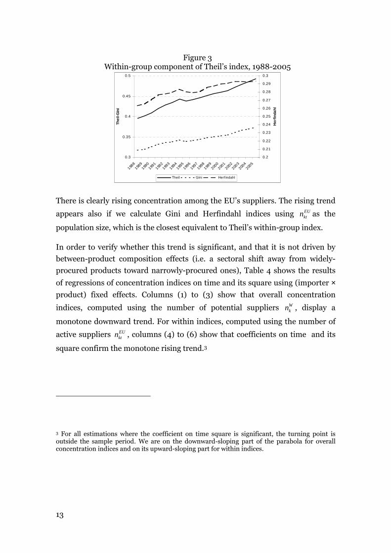
Figure 3 shows the evolution of simple averages over all products of Theil’s
within-group component.
13
Figure 3 Within-group component of Theil’s index, 1988-2005
0.3
0.35
0.4
0.45
0.5
1988
1989
1990
1991
1992
1993
1994
1995
1996
1997
1998
1999
2000
2001
2002
2003
2004
2005
Thei
l-Gin
i
0.2
0.21
0.22
0.23
0.24
0.25
0.26
0.27
0.28
0.29
0.3
Her
finda
hl
Theil Gini Herf indahl
There is clearly rising concentration among the EU’s suppliers. The rising trend
appears also if we calculate Gini and Herfindahl indices using EUktn as the
population size, which is the closest equivalent to Theil’s within-group index.
In order to verify whether this trend is significant, and that it is not driven by
between-product composition effects (i.e. a sectoral shift away from widely-
procured products toward narrowly-procured ones), Table 4 shows the results
of regressions of concentration indices on time and its square using (importer × product) fixed effects. Columns (1) to (3) show that overall concentration
indices, computed using the number of potential suppliers Wkn , display a
monotone downward trend. For within indices, computed using the number of
active suppliers EUktn , columns (4) to (6) show that coefficients on time and its
square confirm the monotone rising trend.3
3 For all estimations where the coefficient on time square is significant, the turning point is outside the sample period. We are on the downward-sloping part of the parabola for overall concentration indices and on its upward-sloping part for within indices.

14
Table 4 Regression results, EU import concentration on time trend
(1) (2) (3) (4) (5) (6)
Theil Overall Hrfal Overall Gini Overall Theil Within Hrfal Within Gini Within
Time 0.001091 0.000992 -0.000778 0.006959 0.002601 0.002866
[1.565] [2.540]** [7.984]*** [11.477]*** [4.836]*** [7.701]***
Time^2 -0.000397 -0.000203 -0.000035 0.000037 -0.000006 0.000088
[11.237]*** [10.268]*** [7.158]*** [1.194] [0.226] [4.675]***
Constant 3.708313 0.724127 0.91898 0.374646 0.258379 0.307514
[1269.443]*** [442.112]*** [2250.572]*** [147.390]*** [114.595]*** [197.090]***
Turning Point 1988 1989 1976 1893 2204 1971
Observations 155290 155290 155290 155334 155334 155334
R-squared 0.768 0.628 0.842 0.71 0.407 0.694
Fixed Effects yes yes yes yes yes yes
How about the extensive margin? Figure 4 shows the evolution of simple
averages over all products of Theil’s between-group component and EU’s
number of suppliers over time.
Figure 4 Extensive margin, 1988-2005
Theil’s index Between component Number of EU countries partners
3.10
3.15
3.20
3.25
3.30
1988
1989
1990
1991
1992
1993
1994
1995
1996
1997
1998
1999
2000
2001
2002
2003
2004
2005
3.5
3.7
3.9
4.1
4.3
4.5
4.7
4.9
1988
1989
1990
1991
1992
1993
1994
1995
1996
1997
1998
1999
2000
2001
2002
2003
2004
2005
NE
Ukt
0.055
0.057
0.059
0.061
0.063
0.065
Alp
ha
NEUkt
Alpha
Note: Simple averages of Theil-between components at the product (HS8) level.
Note: Simple averages of number of exporters to EU at the product (HS8) level.
The downward trend in the between component of the Theil index, along with
the rising number of suppliers, now suggests diversification at the extensive
margin. This is what one would have expected in view of declining
transportation and trade costs (as suggested by the gravity literature), but it is
somewhat conflicting with the rising concentration observed at the intensive
margin.

15
A regression of the between component of the Theil index and the number of
suppliers on a time trend (with, again, importer × product fixed effects) confirms the monotone increase. Table 5 reports the results for pooled and
fixed-effects regressions of the between component of the Theil index and the
number of suppliers to an EU member country on time and its square.
Table 5 Regression results, Theil-between and number of EU suppliers
(1) (2) (3) (4) (5)
Theil Between Theil Between
Nbre Active
Suppliers
Nbre Active
Suppliers
Ln(N Active
Suppliers)
Time -0.000335 -0.005861 0.023829 0.039415 0.0141719
[0.176] [6.575]*** [2.131]** [10.033]*** [66.49]***
Time^2 -0.000315 -0.000434 0.00116 0.001554
[3.267]*** [9.601]*** [2.012]** [7.807]***
Constant 3.265007 3.33285 4.007372 3.808936 0.8659872
[413.271]*** [891.745]*** [87.890]*** [231.277]*** [374.19]***
Turning Point 1986 1980 1977 1974 -
Observations 155334 155334 155334 155334 155334
R-squared 0.001 0.813 0.002 0.899 0.798
Fixed Effects no yes no yes yes
The coefficients in column (5) imply that the number of E.U. suppliers rises by
1,5% a year. This is a slow rise: Given that the average number of suppliers per
product is a little less than 5 for the representative E.U. member, it takes about
14 years for the E.U. to add one more supplier.
So far, thus, we get the following picture: on the one hand, supplier
concentration is rising at the intensive margin, meaning that the largest existing
suppliers get larger relative to the average. On the other hand, concentration is
decreasing at the extensive margin, as more and more suppliers are added—
albeit slowly—to the EU’s portfolio of suppliers. These observations can be
reconciled as follows. Suppose first that a group of three incumbent suppliers
each supply $3 to the E.U., with two more potential suppliers waiting in the
wings with zero exports to the EU. The within Theil index for group 1 (active
suppliers) is zero. Suppose now that one of the two potential suppliers gets in at
a scale of $3. Group 1 enlarges to 4 members, group 0 shrinks to 1 member, and
the within Theil index for group 1 stays at zero.
Consider now a different setup where the three initial incumbents have unequal
export levels; say, $4, $3 and $2 respectively. The group Theil index for group 1
is 0.04. Suppose now that the entrant from group zero enters with exports of
only $1. Then the within Theil index for group 1 rises to 0.2. The reason is that

16
the group is now more unequal, as the largest exporter has 4/2.5 = 1.6 times the
group average instead of 4/3 = 1.33 previously. Thus, there has been
diversification at the extensive margin but the within-group Theil index
calculated on active exporters is showing rising concentration.
That entrants enter small-scale is natural if they are being tested or if they
themselves want to “try the market” small scale before taking big risks (on this,
see e.g. Rauch and Watson 2003). But is it the case that new entrants in the
EU’s portfolio of suppliers are small in world trade? In order to look at this, we
now turn to an adaptation of Hummels and Klenow’s definition of the intensive
and extensive margins.
2.2.2 Using Hummels and Klenow’s decomposition
We use a slightly different definition of the extensive margin due to Hummels
and Klenow (2005, henceforth HK). They defined the intensive and extensive
export margins of country i, product-wise, as
i
i
ikki
Wkk
XIM
X∈ℵ
∈ℵ
=∑∑
(13)
and
i
Wkki
Wkk
XEM
X∈ℵ=
∑∑
(14)
respectively. In words, country i’s intensive margin is its share of world trade in
what it exports (how big it is in what it exports), whereas its extensive margin is
the share in world trade of the products that it exports (how important is what it
exports). The difference between iEM and just counting the active export lines is
that if country 1 exports, say, carrots and potatoes, whereas country 2 exports
cars and computers, they have the same number of active lines, but the
extensive margin measured à la HK would be higher for country 2 because what
it exports is larger in world trade. It is easily verified that multiplying the
extensive margin by the intensive one gives country i’s share in world trade.
We adapt the concept to imports and to a geographical instead of product-wise
measure. In our setting, the equivalents of HK’s intensive and extensive margins
are

17
,
,k
k
i EUki S
k i Wki S
MIM
M∈
∈
=∑∑
(15)
and
,
,k
i Wki S
k i Wki
MEM
M∈=
∑∑
. (16)
That is, product k’s intensive margin for the EU is the EU’s share of its
suppliers’ exports (how big it is in its suppliers’ exports of good k), whereas its
extensive margin is the share of its suppliers in world trade of good k (how
important are its suppliers in good k). Whereas in HK’s case, multiplying the
intensive margin by the extensive margin gives the exporter’s share in world
trade, here it gives the importer’s share in world imports of good k. Our
extensive margin differs from counting the number of supplier countries as
follows. If the EU imports wheat from the US and Australia, and rice from Niger
and the Mali, both products are sourced from two countries. However the US
and Australia are much larger in wheat trade than are Niger and Mali in rice
trade. The extensive margin is, accordingly, higher for wheat than for rice.
Table 6 reports the results of pooled and fixed-effects regressions of the
extensive and intensive margins on time and its square. The negative trend at
the extensive margin is only significant with the introduction of importer × product fixed effects. The decrease in the intensive margin is significant and
robust to the introduction of fixed effects.
Table 6 Regression results, Intensive and Extensive margins of EU country imports
(1) (2) (3) (4)Extensive
Margin
Extensive
Margin
Intensive
Margin
Intensive
Margin
Time -0.000029 -0.007404 -0.020632 -0.020213
[0.024] [10.934]*** [23.982]*** [37.906]***
Time^2 -0.000047 0.000309 0.000777 0.000745
[0.830] [9.884]*** [20.650]*** [30.260]***
Constant 0.537564 0.567948 0.200292 0.200116
[88.946]*** [170.718]*** [44.286]*** [76.385]***
Observations 78665 78665 78665 78665
R-squared 0 0.737 0.019 0.493
Fixed Effects (Importer*product) no yes no yes
* significant at 10%; ** significant at 5%; *** significant at 1%
Absolute value of t statistics in brackets

18
However, econometric results must be interpreted very cautiously here. Figure 5
shows fitted curves corresponding to columns (2) and (4) of Table 6. They head
down only between 1988 and 1994-5, during which the COMTRADE database
was progressively enlarging to new countries. Once COMTRADE reaches
steady-state, there is no trend anymore. We take this to be the correct answer to
our question.
Figure 5 Predicted HK’s intensive and extensive margins, 1988-2005
0 .4 0
0 .4 5
0 .5 0
0 .5 5
0 .6 0
1 9 8 8 1 9 9 0 1 9 9 2 1 9 9 4 1 9 9 6 1 9 9 8 2 0 0 0 2 0 0 2 2 0 0 4
EX
ten
sive
Mar
gin
0 .1 0
0 .1 5
0 .2 0
0 .2 5
0 .3 0
0 .3 5
Inte
nsi
ve M
arg
in
IM E M
The flat trend of the extensive margin over 1995-2005 suggests that the
combined share of EU suppliers in world trade is constant, even though their
number is growing. That is, newcomers into EU supply chains are so small in
world trade that they make no difference in the extensive margin. This confirms
our interpretation of the rise in the group-1 (active-exporters) value of Theil’s
index: inequality is rising among EU suppliers, not because large suppliers
acquire increasingly dominant positions, but because small suppliers keep on
coming on a very small scale.
All in all, in spite of the rise in Theil indices among active suppliers, the picture
we get is one of increasingly diversified geographical sourcing, albeit by
addition of a fringe of very small exporters. We now turn to an analysis of the
relationship between public-health concerns and the concentration and identity
of EU suppliers.

19
3. Do food alerts cause supplier concentration?
Trade theory predicts that if trade costs go down or if productivity rises
exogenously in a pool of potential suppliers with heterogeneous productivity
levels, the number of suppliers will enlarge (Helpman, Melitz and Rubinstein
2008). An exogenous taste for variety, or a desire to limit monopoly positions,
would also lead to a larger number of suppliers, although these forces are static.
In the presence of heterogenous quality, however, the dynamics of
diversification/concentration can be different.
As new exporting countries get on the EU’s list of suppliers of good k, they need
to build a reputation of quality for their products. The value of information on
the level of health risk of a good k drives the search for quality. There is then a
trade-off between concentrating on top quality suppliers and keeping several
suppliers in order to “test” them.
3.1 The food alert data
We use Eurostat’s Rapid Alert System for Food and Feed (RASFF). The RASFF
is a system of notification and information exchange on emergency sanitary
measures taken at the border by EU member states in place since 1979. The
database we use records all notifications (19’000 of them) between 2001 and
2008 with the identity of the importing EU member state, exporting country,
product, hazard, type of notification, and type of measure. Notifications can be
of two types: “information” or “alerts”. In the former case, the hazard is deemed
limited; the importing member state imposes a measure (e.g. destruction of the
shipment) and informs the rest of the Community of the problem, but other
members do not follow suit. In the latter case, the hazard is deemed sufficiently
serious to warrant action at the Community level. Measures are thus taken
simultaneously by all member states against the exporting country for the
product concerned.
The database contains complete information regarding products, but in verbal
form, as products are not coded into the HS system. We painstakingly coded all
incriminated products into HS8 categories over the period 2001-2005 (8’895
observations), and created an entirely new database, which we now briefly
describe.
Figure 6 shows the evolution over time of the number of notifications (including
informations and alerts). Informations outnumber alerts by a ratio of more than

20
four to one, and represent 82% of all notifications. Both informations and alerts
show a sharply rising trend, although somewhat decelerating for informations
after 2003.
Figure 6 Total SPS, Alerts and Information notifications, between 2001-2005
0
500
1000
1500
2000
2500
2001 2002 2003 2004 2005
All
Informations
Alerts
There is substantial prima-facie heterogeneity among notifying EU states in the
frequency of notifications. Germany (25% of observations), Italy (21%) and
Spain (17%) are the top notifying countries, while Ireland accounts for only
0.61% of them. Figure 7 shows that there is also heterogeneity in terms of
products. Fishery products (30%), Fruit and Nuts (23%) and Coffee & Herbs
and spices (10%) rank highest in terms of reported notifications.
Figure 7 Main Sectors concerned by SPS notifications
0%
5%
10%
15%
20%
25%
30%
35%
40%
Meat
Fish
Dairy produce
PAO nes
Vegetables
Fruit & nuts
Coffee, tea
Cereals
Milling industry
Oil seeds
Vegetable plaiting
Animal or vegetable fats
Prep of meat, fish
Sugars
Cocoa
Prep of cereals
Prep of vegetables etc
Miscellaneous
% #
Ale
rts
2001
2005
Avg All years
Note: Simple average of the number of notifications at the product (HS8) level
In terms of hazards, considering all years and importers, the main cause of
notifications for agricultural products is contamination by mycotoxins (mainly

21
aflatoxin), which alone accounts for 40% of the notifications. The second cause
is contamination by residues of veterinary medicinal products
(chloramphenicol, nitrofuran, and tetracycline) which together account for 13%
of the notifications. Then comes the presence of pathogenic micro-organisms
(10%) and contamination by pesticide residues (3%).
The dataset also details the action taken after each notification. Overall, 92.7%
of notified shipments are stopped at the border. In 42.2% of the cases, they are
destroyed. The rest (50.5%) are re-dispatched to other destinations; that is, they
do not penetrate the EU market but will nevertheless end up in somebody’s
mouth. An additional 0.4% of imports are banned (Table 7). Thus, whether
alerts or informations, notifications are extremely restrictive.
Table 7 Main actions taken following notifications, 2001-2005
Info Alert Info Alert Info Alert Info Alert Info Alert Total %
Physical treatment 0 0 1 0 6 0 27 2 61 0 97 1.3%
Product seized &
destroyed 264 66 614 131 616 109 410 222 451 353 3236 42.2%
Product re-dispatched120 31 197 28 1049 29 1189 44 1137 56 3880 50.5%
Ban 0 0 1 2 1 0 4 5 7 12 32 0.4%
Reinforced checking &
screening 9 1 6 5 17 0 5 0 40 4 87 1.1%
Others 6 0 44 6 54 10 106 11 72 36 345 4.5%
Total 399 98 863 172 1743 148 1741 284 1768 461 7677 100%
2001 2005200420032002
The level of sanitary risk associated with imported agri-food products can result
from (i) intrinsic product characteristics, as some products are more vulnerable
than others to contamination, (ii) supplier characteristics, as some producers
are more able than others to apply necessary controls, or a combination of both.
Figure 10 shows a scatter plot of exporter shares in notifications against their
share in EU imports, both in logs and averaged over years and products. Along
the diagonal, China, Turkey and Brazil are most affected by SPS notifications,
but they are also the EU’s largest suppliers. Dispersion around the diagonal is
substantial; countries like Poland, Hungary or the US are large exporters, but
subject to relatively few notifications; at the other end of the spectrum, Vietnam,
India and Indonesia suffer a disproportionate number of notifications given
their relatively lower import shares.

22
Figure 10 Mains exporters concerned by SPS notifications, all years and products
Nor
Swe
Swi
Tur
Est
La t
Pol
Cze
Hun
Rom
BulUkr
Mol
Ru sUzb
Mo r
Tun
Egy
Mau
Ma l
B ur
Sen
Ivo
Gh a
Tog
Ben
Nig
Cam
C on
Tan
Se ySou
Nam
Usa
Pan
SurEcu
Per
B ra
ChiPar Uru
Arg
Cyp
Le b S yr
Ira Isr
Pak
Ind
Ban
Sri
Mya
Th aV ie
Ind
Ma l
Ph i
Chi
SouJap
Hon
Aus
N ew
Fij-8
-6-4
-2Ln
Ale
rt
-8 -6 -4 -2Ln ImpShare
The dispersion around the diagonal suggests that important country-specific
characteristics, over and above their sales volumes, affect the number of times
their exports are affected by notifications. These characteristics include of
course the product composition of their exports, but they may include as well
characteristics of national production systems which must be taken into account
when assessing the level of product-specific sanitary risk.
In the econometric analysis that follows, we combine the RASFF database with
the EUROSTAT data on EU agri-food imports analyzed in the first part of this
paper. The sample period is restricted to 2001-2005 where both trade and
notification data are available.
3.2 Product risk and concentration
As explained in the introduction, we use a two-stage procedure where observed
product riskiness, used as explanatory variable in the second-stage regression, is
estimated in a first-stage auxiliary regression. The procedure goes like this:
Step 1.
For a product k and an exporter i, the dependent variable is ikA , the combined
count of notifications from all EU member states between 2001 and 2005. Thus,
the unit of observation is an exporter × product pair and the regression is cross-sectional. Regressors include ikS , exporter i’s initial share in EU imports of
product k; kτ , the ad-valorem equivalent of the EU’s MFN tariff on product k;

23
kQ , a dummy variable indicating whether product k is affected by a quota
during the sample period; kD , a dummy variable indicating whether product k
has been the object of a dispute at the WTO between the EU and any other
country. Variables kτ , kQ , and kD control for a possible protectionist agenda.
We also include kB , a dummy variable indicating whether exporter i is affected
by a ban on product k during the sample period. kB controls for decreases in the
incidence of notification resulting from reduced imports rather than reduced
risk. Finally, the regression includes product and exporter effects kδ and iδ .
Formally,
( )0 1 2 3 4ik k k k k i k ikA f Q D B uα α τ α α α δ δ= + + + + + + + (17)
where iku is an error term. Because the number of notifications is a count (with a
huge proportion of zeroes), estimation is by Poisson or negative binomial.4
We also control for the initial value of EU imports of product k in the year 2000
(one year before the sample start), as products imported in large volumes are
likely to be inspected (and therefore to fail inspections) more often than others.5
Step 2.
Estimated coefficients on product dummies, k̂δ , are retrieved from Step 1 and
used as explanatory variables in a panel regression of concentration indices,
where the unit of observation is a product × year pair.6 That is, the second-stage equation is
4 This is largely inconsequential, as consistency of second-stage estimates does not depend on the correct specification of the first-stage equation.
5 This is done using the “exposure” option for count models in STATA, which is equivalent to including the initial volume of imports as a regressor with a coefficient constrained to be one.
6 When estimated coefficients were not significant at the 10% level, they were set equal to zero.

24
0 1 2 3 4 5 6ˆ ˆ
kt k k k k t k t ktC Q D vβ β τ β β β δ β δ β δ δ= + + + + + + + (18)
where ktC is a measure of concentration (within- and between-groups
components of Theil’s index, or simple number of suppliers) for good k in year t
and other variables are as before, except for time effects tδ which enter the
equation both linearly and interacted with product-risk estimates from Step 1.
4.2.3 Results
First-step regression results yielded over two thousand estimated product
coefficients. The distribution of significant point estimates is shown in Figure 8.
Figure 8 Distribution of significant point estimates on product dummies
Game fresh or frozen meat
Fresh or chilled pacific salmon
Fresh or chilled fillets f ish
Frozen fillets of cod
Tuna
Frozen shrimps and prawns
Mussels
Sinews or tendons
Dried vegetableswalnuts
pistachios
fruits and nuts
Coffee
Crushed Chili
Soya beans
Ground-nuts
Shelled ground-nuts
Sunflower seeds
Poppy seeds
Crude palm oil
Sesame oil
Bovine meat prep
preserved fish
Crustaceans prepsweets
tablets
Cocoa beans
biscuits
Preserved vegetables
AsparagusOlives
Nuts and other seeds
tomato saucesMustard
Food preparations
02
46
810
coe
ffici
ent N
ega
tive
bino
mia
l
0 1 2 3 4 5 6 7 8 9 10 11 12 13 14 15 16 17 18 19 20 21hs2
It can be seen that no chapter stands out as having particularly high risk levels,
except for fisheries products, with mussels as an unsurprising outlier. It is also
remarkable to see that traditional tropical products such as coffee and cocoa,
whose share in EU foodstuff imports is, as noted, declining, are among the
safest.

25
Second-step regression results are shown in Table 8.
Table 8 Regression results, second stage
(1) (2) (3)
Theil Within Theil Between Nber Suppliers
Product risk a/ 0.044*** -0.128*** 1.638***
(6.427) (-12.033) (13.224)
risk*Time b/ 0.088*** -0.044** 0.796***
(7.345) (-2.340) (3.645)
Tarrif_2005 c/ 0 0 -0.010*
(1.091) (-0.550) (-1.779)
Quota_2005 d/ -0.212*** 0.357*** -2.220***
(-9.853) (10.580) (-5.672)
Ban e/ -0.350*** 0.562*** -5.308***
(-24.094) (24.676) (-20.073)
Dispute f/ -0.093 0.142 -0.901
(-1.369) (1.340) (-0.731)
Imports g/ 6.15e-10*** -9.57e-10*** 1.87e-08***
(13.903) (-13.826) (23.289)
Constant 1.076*** 2.070*** 12.765***
(102.057) (125.346) (66.551)
Observations 7051 7051 7051R-squared 0.219 0.232 0.263
Time fixed effects yes yes yes
t-statistics in parentheses, *** p<0.01, ** p<0.05, * p<0.1
Note: a/Product risk coefficient estimated in step1 b/Interaction term between time variable and a risk dummy variable, that takes the value 1 if for the product risk coefficient is positive c/Ad-valorem equivalent of protection measures for product k in 2005 d/Dummy variable that takes the value 1 if the product was imposed a quota measure in 2005 e/Dummy variable that takes the value 1 if the product was imposed a ban between 2001 and 2005 f/Dummy variable that takes the value 1 if a trade concern was reported for the product between 2001 and 2005 g/ EU imports of product k , in thousand euros
The dependent variable is the within-groups component of the Theil index (the
intensive margin) in column (1), its between-groups component (the extensive
margin) in column (2), and the number of suppliers in column (3). Coefficients
of our constructed measure of product risk are all highly significant (at the 1%
level), confirming that product riskiness seems indeed to affect sourcing
concentration.
Thus, again, the evidence points in conflicting directions. On one hand, column
(1) suggests that concentration is higher at the intensive margin for riskier
products. On the other hand, column (2) suggests that concentration is lower at
the extensive margin for those products, and column (3), that the number of

26
suppliers is higher. We already observed, in Section 2, that the distribution of
EU suppliers was evolving precisely in that direction—concentration at the
intensive margin and diversification at the extensive margin. Thus, combining
our results in Section 2 with those of the present section, it seems that the
distribution of EU suppliers is converging toward the pattern that we observe
for the riskiest products—increasingly dominant suppliers with a growing fringe
of small-scale ones.
Figure 9 shows the first and last quartile import share distribution in 2005 for
risky versus safe products. Risky products are products with a positive risk
coefficient. For the smallest partners ( last quartile of the import share
distribution), the risky products distribution is shifted to the compared safe
products. While for the biggest exporters ( first quartile of the import share
distribution) the curves are very similar and no shift in either direction is
observed. Thus, there is a rising polarization between the bottom and the top of
the distribution for risky products.
Figure 9 Import share distribution for risky and safe products, 2005
Smallest exporters, last quartile Biggest exporters, first quartile
0.0
5.1
.15
.2.2
5kd
ensi
ty ln
Q4
-15 -10 -5 0Ln(4thQuartileImport Share)
Safe ProductRisky Product
02
46
810
kden
sity
lnQ
1
-1.5 -1 -.5 0Ln(1stQuartileImport Share)
Safe ProductRisky Product

27
5 Concluding remarks
This paper establishes a stylized fact on EU import concentration in agro-food
products and a correlation with the degree of product safety. We have shown
that EU imports of agro-food products over 1988-2005 show a pattern of
concentration at the intensive margin and diversification at the extensive
margin, the more so for products that EU deemed risky, as demonstrated by the
number of food alerts that occurred on that product between 2001 and 2005.
While previous empirical work have focused on the ex-ante impact of standards
on trade flows, this paper is, to our knowledge, the first to assess the impact of
standards on trade flows ex-post. Using a new dataset - that has never been
exploited before- on food alerts that can provide information on the effective
(ex-post) implementation of SPS norms by EU importing countries, this paper
contributes to the empirical debate about the evolution of geographical
concentration of agrofood imports across time. The empirical results are clear.
European importers tend to procure their agrofood products from an
increasingly large portfolio of suppliers but large orders are concentrated on few
among this pool of suppliers.
The policy implications of these results are of significant interest. Indeed as EU
foodstuff distributors show growing concerns for food safety, the access to EU
markets developing countries enjoy may be constrained by increasingly
stringent sanitary requirements. While almost all papers address the issue of
developing countries exports opportunities from the exporting country
viewpoint, we consider it from the importer point of view. Developing countries
export opportunities especially for high-value food products -fresh and
processed fruits and vegetables, fish, meat, nuts, and spices- are shaped by
importers requirements. Therefore understanding how the implementation of
sanitary standards may affect importers suppliers selection is of critical
importance for developing countries to maximise the magnitude of these
opportunities.

28
References
Amurgo-Pacheco, Alberto, and M. D. Pierola (2008), "Patterns of Export
Diversification in Developing Countries: Intensive and Extensive Margins",
Policy Research Working Paper No. 4473, The World Bank.
Besedes, T. and T. Prusa (2006a), “Surviving the U.S. Import Market: The Role
of Product Differentiation”, Journal of International Economics 70, 339-358.
− and − (2006b), “Ins, Outs, and the Duration of Trade”, Canadian Journal of
Economics 39, 266-95.
Brenton, Paul, J. Sheehy, and M. Vancauteren (2001), “Technical Barriers to
Trade in the European Union: Importance for Accession Countries”, Journal of
Common Market Studies, 39(2), 265-284.
Carrère, Céline, V. Strauss-Kahn and O. Cadot (2007), “Export Diversification:
What’s Behind the Hump?”; mimeo, University of Lausanne.
Campa, Jose Manuel and L. Goldberg (1997), “The Evolving External
Orientation of Manufacturing Industries: Evidence from Four Countries”;
NBER Working Paper #5919.
Disdier, Anne-Célia, L. Fontagné, and M. Mimouni (2007), “The Impact of
Regulations on Agricultural Trade: Evidence from SPS and TBT Agreements”,
Working Paper No. 2007-04, CEPII.
Ethier, Wilfred (1982), “National and International Returns to Scale in the
Modern Theory of International Trade”; American Economic Review 72, 389-
405.
− (1998), “Regionalism in a Multilateral World” ; Journal of Political Economy
106, 1214-1245.
European Commission (2005), “Guidance Document on certain key questions
related to import requirements and the new rules on food hygiene and on
official food controls.”
European Commission (2000), “Guide to the Implementation of Directives
Based on the New Approach and the Global Approach”,
http://europa.eu.int/comm/enterprise/newapproach/newapproach.htm.

29
Fontagné, L., Mimouni, M., Pasteels, J.M., 2005, “Estimating the Impact of
Environmentally –Related Non-Tariff Measures.” World Economy, 28(10):
1417-1439.
Fujita, Masahiro; P. Krugman and A. Venables (1999), The Spatial Economy;
MIT Press.
Garcia-Martinez, Marian, and N. Poole (2004), The development of private
fresh produce safety standards: implications for developing Mediterranean
exporting countries; Food Policy 29, 229-255.
Hausmann, R. and D. Rodrik (2003), “Economic Development as Self-
Discovery”; Journal of Development Economics 72, 603-633.
−, J. Hwang and D. Rodrik (2005), “What You Export Matters”; NBER working
paper 11905.
Imbs, Jean, and R. Wacziarg, 2003, "The Stages of Diversification", American
Economic Review, 93(1), 63-86.
Jaffee, Steven (2003), “From Challenge to Opportunity: Transforming Kenya’s
Fresh Vegetable Trade in the Context of Emerging Food Safety and Other
Standards in Europe,” Agriculture and Rural Development Discussion Paper 1,
World Bank.
Jaffee, Steven, and S. Henson (2004), “Standards and Agro-Food Exports from
Developing Countries: Rebalancing the Debate,” World Bank Policy Research
Paper No. 3348. World Bank.
Jaffee, Steven, and al. (2005), “Food Safety and Agricultural Health Standards:
Challenges and Opportunities for Developing Country Exports,” Report no.
31207, Poverty Reduction & Economic Management Trade Unit and Agriculture
and Rural Development Department, World Bank.
Klinger, Bailey and D. Lederman (2004), “Discovery and Development: An
Empirical Exploration of ‘New’ Products; mimeo.
− and − (2005), “Diversification, Innovation, and Imitation off the Global
Technology Frontier”; mimeo.
Lorenzo Cappellari & Stephen P. Jenkins, 2004. "Modelling Low Pay Transition
Probabilities, Accounting for Panel Attrition, Non-Response, and Initial
30
Conditions," CESifo Working Paper Series CESifo Working Paper No. , CESifo
GmbH
Maskus, K.E., Wilson, J.S., Otsuki, T. (2000), “Quantifying the Impact of
Technical Barriers to Trade. A framework for Analysis.” Mimeo, World Bank.
Maskus, K.E., Otsuki, T., Wilson, J.S. (2005), "The cost of compliance with
product standards for firms in developing countries: an econometric study."
Policy Research Working Paper Series 3590, The World Bank.
Moenius, Johannes ( 2006), “The Good, the Bad, and the Ambiguous:
Standards and Trade in Agricultural Products”, Paper presented at the IATRC
Summer Symposium, Bonn, May 2006, http://www.agp.uni-
bonn.de/iatrc/iatrc_program/Session%203/Moenius.pdf.
Otsuki, T., Wilson, J.S., Sewadeh, M., (2001), “Saving Two in a Billion:
Quantifying the Trade Effect of European Food Safety Standards on African
exports.” Food Policy, v-26, pp.495-514.
Plaggenhoef, W. van ,M. Batterink and J. H. Trienelkens (2002), “International
Trade and Food Safety: Overview of Legislation and Standards,” Global Food
Network
Rauch, James, and J. Watson (2003), “Starting Small in an Unfamiliar
Environment,” International Journal of Industrial Organization, 21, pp. 1021-
1042.
World Bank (2005), “Food Safety and Agricultural Health Standards:
Challenges and Opportunities for Developing Country Exports”; Poverty
Reduction & Economic Management Trade Unit and Agriculture and Rural
Development Department Report 31207.
Related Documents