Do EU15 countries compete over labour taxes?

FACULTEIT ECONOMIE EN BEDRIJFSKUNDE

TWEEKERKENSTRAAT 2 B-9000 GENT

Tel. : 32 - (0)9 – 264.34.61 Fax. : 32 - (0)9 – 264.35.92

WORKING PAPER

Do EU15 countries compete over labour taxes?

Bruno Merlevede

Glenn Rayp

Stefan Van Parys

Tom Verbeke

October 2011

2011/750

D/2011/7012/55

Do EU15 countries compete over labour taxes?∗

Bruno Merlevede† Glenn Rayp‡ Stefan Van Parys§ Tom Verbeke¶

October 25, 2011

AbstractEmpirical research on international tax competition has mainly considered cor-

porate taxation. Because of the limited international mobility of labour, labour taxcompetition tends to be overlooked. This may be unjustified. The tax base in labourtaxation is the wage mass that depends on employment. While labour is largely in-ternationally immobile, jobs are certainly not because of the international mobilityof goods. Given the higher share of labour tax in government revenues, labour taxcompetition could also have more important welfare consequences than corporate taxcompetition. We model the possibility of labour tax competition using a standardDixit-Stiglitz two-country model with immobile firms and workers and transportationcosts in exporting goods. The model is extended with the assumptions of non-clearinglabour markets and income redistribution by the government, financed by a labour tax.The model results in an empirical specification of the labour tax reaction function inthe form of a spatial lag panel. The tax reaction function is then estimated for theEU15 member states using an instrumental variable approach. Our results point tothe presence of small, but significant labour tax competition within the EU15.

JEL Classification: H0, H25, H77Keywords: tax competition, labour tax, spatial autocorrelation, strategic interactions.

∗This research is part of the ANR project MONDES. Financial support by the ANR is gratefully ac-knowledged†Ghent University and HUBrussel‡Ghent University and SHERPPA§Ghent University¶HUBrussel, Ghent University, and C.E.S. KULeuven

1

1 Introduction

In the past, the empirical research on tax competition almost exclusively considered the local

or regional policy level (see Brueckner, 2003). In the last ten years, however, an increasing

number of studies analyses tax competition between countries, in particular between EU-

members. These studies consider the question whether market integration and the removal

of barriers to factor mobility has induced EU-members to set tax rates strategically.

In line with the definition of Wilson and Wildasin (2004) of tax competition as "...non-

cooperative tax setting by independent governments under which each government’s public

choices influence the allocation of a mobile tax base among ’regions’represented by the gov-

ernments..." in short "competition for mobile factors", empirical research on international

tax competition has almost exclusively considered corporate taxation because of the high

international mobility of firms (capital) relative to workers. Competition in the taxation

of immobile production factors is neglected in almost all theoretical and empirical studies,

with Altshuler and Goodspeed(2003) at the empirical and Andersen (2003) at the theoretical

level as notable exceptions. We see, however, at least three arguments why the analysis of

labour tax competition is important, even if labour is a to a large extent immobile production

factor1.

• While labour may be immobile, because of goods or capital mobility jobs are not.To the extent that jobs’mobility depends on production costs, labour taxation will

influence the allocation of jobs through wage costs.

• Corporate taxation represents only a limited share of government revenue in the in-dustrialised countries. Hence, the effects on the level of provision of public goods or on

the distortion of the tax structure of a suboptimal level of corporate taxation due to

corporate tax competition could be rather small. The welfare consequences of labour

tax competition, on the other hand, could be far more considerable given labour tax’s

weight in government finance.2

• Taxation of immobile production factors is seen as the possible synthesis of the "com-pensation" and the "effi ciency" hypotheses concerning globalization and public spend-

ing (social security spending in particular). Since Rodrik (1997) the relation between

globalization and social protection is considered in terms of two contradicting tenden-

cies. On the one hand, globalization may increase the demand for social spending as

1See also Andersen (2003) for similar arguments2In 2007, at the level of the EU15, taxes on labour represented about 45% of total taxation (based on

European Commission, 2009)

2

compensation for the increased risks of unemployment and income inequality. On the

other hand, globalization may constrain the government in raising the necessary funds

for social compensation because of increased capital mobility. The "synthesis" of the

two hypotheses is therefore a higher taxation of immobile production factors (labour).

This synthesis would be obstructed, however, if globalization induces governments to

set labour tax rates strategically.

We notice two strands in the literature on the empirical relation between economic inte-

gration and tax policy at the national level. The first strand in the literature attempts to

estimate tax reaction functions, while the second analyses the effect of globalization, proxied

by an openness indicator, on tax receipts or public spending in a reduced form regression

framework. This difference almost parallels the distinction in the literature between the

analysis of corporate taxation using the reaction function approach (e.g. Bénassy-Quéré et

al 2007, Casette and Paty 2008, Davies and Voget 2008, Devereux et al. 2008, Redoano

2007) and the analysis of social protection spending using the globalization impact approach

(e.g. Bretscher and Hettich 2002, Dreher 2006, Garrett and Michell 2001, Haufler et al.

2009, Rodrik 1997).

We follow the first approach because of its better theoretical foundation through its link

with a structural model of tax competition. Labour tax reaction functions of the EU15

countries are estimated in a spatial econometrics framework. We focus on the EU for three

reasons. First, the EU is characterised by an unprecedented and far-reaching economic in-

tegration of both goods and capital markets in the last decades (e.g. the Single Market

Program). Second, an EU-focus allows for comparison of our results with existing literature

that has mainly used EU-data to estimate (corporate) tax reaction functions at the coun-

try level. Finally, tax competition and the threat of race-to-the-bottom tax dynamics are

intensively debated and thus highly policy-relevant for the EU.

In the next section, we give a brief presentation of the theoretical model from which

we derive the hypothesis to be tested. The definition of the elements of the spatial weight

matrix in the estimations also follows from our theoretical model. Since Anselin (1988)

the importance of a judicious choice of the weighting scheme, in particular its theoretical

consistency, has been repeatedly stressed (see e.g. Davies and Voget, 2008). In the third

section, we discuss the empirical model specification and the data used for estimation. In

the fourth section, the estimation methodology and the estimation results are dealt with.

Finally, the fifth section concludes.

3

2 Theoretical background

To our knowledge, the theoretical literature on (immobile) labour tax competition is quite

limited, with Andersen (2003) a one of the exceptions. Because of the lack of a standard theo-

retical framework in the literature, we develop the analytical model on which our estimations

are based in this section.

We consider the possibility of labour tax competition using a standard Dixit-Stiglitz two-

country framework with transportation costs in exporting goods and immobile workers and

firms, to which we add the assumption of non-clearing labour markets and the possibility

of equilibrium unemployment. In this framework, tax competition is intuitively conceivable

as follows. Because of unemployment, the government may want to redistribute income by

providing unemployment allowances that are financed by a tax on labour. The labour tax

affects the wage cost and hence the output prices and the market shares of firms. Firms’

market shares determine production and employment. Assuming that the government con-

siders the foreign tax rate as independent from its decisions, it will set a tax rate below the

pareto optimum because it does not take into account the implications of its tax decisions

for foreign social welfare. This results in strategic complementarity of the tax rates.

More formally, based on Rayp and Vanbergen (2009), we use a modified version of the

footloose capital (FC) model of Martin and Rogers (1995) to which we add unemployment

via effi ciency wages and an optimizing government that provides unemployment benefits.

There are two regions, north (N) and south (S), that are symmetric in terms of consumers’

tastes, technology, openness to trade and factor supplies. Each region is endowed with a

fixed number of immobile consumers L. As is custom in a FC-setting, we assume that

each region has half of the worldwide capital endowment (KW ): sK = KKW

= 12. The north

(south) produces nN (nS ) units of differentiated goods under increasing returns to scale

using a linear technology. Because we consider symmetric regions nN = nS = n and hence

sN =nNnW

=nN

(nN + nS)= 1

2. More specifically, we assume that the production of each

variety i requires a fixed amount k (= 1) of capital and a variable unit input requirement

involving1

a(wi)units of labour li. a(wi) indicates the worker’s effort as function of the wage

received. The total output of a firm xi equals a(wi)li and the total cost function for a variety

i is equal to πi + liwi, with πi and wi respectively are equal to the reward to capital and to

labour. The export of goods is inhibited by iceberg type of trade costs which imply that τ

(> 1) units have to be shipped to get one unit at destination. Market clearing implies that

the total production of a (northern) firm xN is equal to the sum of the total consumption of

its good in the north CNN and total consumption in the south CNS multiplied by the trade

costs: xN = CNN + τCNS.

4

2.1 Consumers’choice

The optimization problem for a northern consumer with an expenditure level e who consumes

an amount ci (at the price piN) of a good i is given by:

max (U) = (

∫ nN+nS

0

cσ−1σ

i di) (1)

s.t.∫ nN+nS

0

piNcidi = e.

Standard utility maximization and aggregating the j consumers’demand lead to the following

result for the northern market demand of a variety i

CiN = (piNPN

)−σ(ENPN

). (2)

where EN stands for the total northern expenditures and PN = (∫ nN+nS0

p1−σiN di)1

1−σ is the

northern price index.

2.2 Producers’choice

Under the Chamberlinian large group assumption, profit maximization by a northern firm

leads to the well-known determination of the price the firm applies in the north (south)

pNN (pNS) as a fixed mark-up over marginal labour costs in the north and transportation

costs:

pNN =σ

σ − 1

wNa(wN)

, pNS =σ

σ − 1

wNa(wN)

τ = τpNN . (3)

Similar mill pricing applies for the prices charged by southern firms. Based on these expres-

sions, we can work out the (northern) price index:

PN = αwS

a(wS)(ε+ φ

2)

11−σ = α

wSa(wS)

∆1

1−σN . (4)

with α = σσ−1n

11−σW . φ = τ 1−σ represents the well-known freeness of trade and ε = (wN/a(wN )

wS/a(wS))1−σ

is a function of the relative unit production cost wN/a(wN )wS/a(wS)

. When the north has lower (higher)

production costs than the south, ε is larger (smaller) than 1. So ε can serve as a measure

of the competitiveness of the northern region relative to the southern region. We also intro-

duced the short-hand notation3 ∆N .

3Similarly to ∆N , we also define ∆S = (1 + εφ

2)

5

Next, we determine the sales of a firm in function of the share of expenditures sE. The

total sales of a northern firm SN equals the sum of its sales in the north (pNNCNN) and the

south (pNSCNS). Using (3) and (2) it is easily derived that the northern sales equals:

SN =EWnW

ε

[sE∆N

+φ(1− sE)

∆S

]=EWnW

BN , (5)

This result and our technology assumption lead to a very simple expression for the north-

ern operating profit OPN = SN −wN lN = EWσnW

BN . Since physical capital is only used in the

fixed cost component of industrial production (and k = 1), the operating profit of a typical

variety is also equal to the reward to capital4.

πN =EWσnW

BN =EWσnW

ε

[sE∆N

+φ(1− sE)

∆S

]. (6)

2.3 Labour market and share of expenditures

We introduce unemployment via an effi ciency wage mechanism. In its fair wage form, this

hypothesis has been used in recent work to analyse the impact of labour market imperfections

on the wage and unemployment effects of international trade (e.g. Kreickemeier and Nelson

2006, Helpman and Grossman 2007) or on economic agglomeration (Egger and Seidel, 2008).

Given that worker heterogeneity is not crucial to our analysis, we simplify the analysis by

assuming that the delivered effort by a worker is positively related to the difference between

the net wage wN(1− zN) and some reference wage wR (Stiglitz, 1976; Summers, 1988):

a(wN) = (wN(1− zN)− wR)β, (7)

in which zN represents the tax rate set by the northern government on gross wages wN . The

strength of the productivity enhancing effect of higher wages is characterized by β and lies

between 0 and 1. The reference wage wR represents the outside option for the worker.

(Northern) Firms determine the wage wN employees receive by maximizing their profit.

The first-order condition resulting from this optimization is the well-known Solow condition

(Akerlof and Yellen, 1986) that states that the elasticity of the effi ciency function with

respect to the wage equals one:wN

∂a(wN )∂wN

a(wN)= 1. (8)

The firm keeps hiring additional people as long as the wage per unit of effort is falling.

4Southern capital reward equals πS = EWσnW

BS = EWσnW

[φsE∆N

+ (1−sE)∆S

]

6

Substituting (7) in (8) leads to the wage paid to northern employees wN :

wN =wR

(1− β)(1− zN). (9)

A similar expression holds for the southern region. Net wages are invariant to tax rates

and only depend on the effi ciency enhancing effect and the reference wage. Hence, for

given reference wages and productivity parameter(s), the competitiveness variable ε and the

relative product prices will only depend on the tax decisions of the governments and the

trade freeness φ.

The amount of labour each firm employs is easily derived from the zero pure-profit condi-

tion as lN = (σ−1)πNwN

. Assuming that all inhabitants of a region (inelastically) supply labour

and confining our analysis to situations where labour supply exceeds demand, we can write

the unemployment rate as uN = 1− nlNL, which equals, using the definition of the amount of

labour each firm employs lN and the wage wN :

uN = 1−(σ − 1)(1− β)nW

2

LwR(1− zN)πN . (10)

Next, we determine the share of expenditures sE. There are no savings, which implies

that the total expenditures of a region are equal to its total income. We distinguish two

components of the regional income: the income of the employed and unemployed, and the

total capital reward. The combined (northern) income of labourers and unemployed is equal

to TLRN = nlNwN(1−zN)+(L−nlN)bN , in which bN stands for the northern unemployment

benefit. Applying the balanced budget restriction of the government and the expression for

the employment level in a northern firm, lN = (σ−1)πNwN

, allows us to rewrite TLRN in terms

of the northern capital reward:

TLRN = nlNwN = (σ − 1)nW2πN . (11)

The second component of total regional income is the capital reward that accrues to the

residents of a region. Assuming that half of the capital used in each region belongs to the

northern capital owners regardless of sN (this follows Martin and Rogers, 1995), each unit of

capital earns the world average reward to capital ACRN = TCRN+TCRSKW

, with TCRN = nπN

(TCRS = nπS) the total northern (southern) capital reward. Substituting the expressions

for the capital reward in ACRN and multiplying this with the total number of units of capital

owned by the north, K gives us the following result for total (northern) capital reward:

TCRN =EW2σ

. (12)

7

Given both components of income (or expenditures) in a region and using (6), the share of

expenditure is easily derived as:

sE =TCR + TLR

EW=

1

2σ(1 + (σ − 1)BN). (13)

Substituting BN in (5) and solving for sE gives a closed-form expression for the northern

share of expenditures:

sE =(ε+ φ) ((2σ − 1) εφ+ 1)

2[σ (ε+ φ) (1 + εφ)− ε(σ − 1)(1− φ2)

] . (14)

(14) implies that (for given demand elasticity and effi ciency wage parameters) the expen-

diture share will only depend on the tax rates and the trade freeness. Hence, in particular

from (6) and (10), it follows that all the variables in the model are determined by the taxation

decisions in the two countries and the trade freeness

2.4 Redistribution and tax competition

For simplicity, the amount of taxes is determined by maximizing an ad hoc social welfare

function in which the indirect utility of the unemployed is given a relative weight γ. In our

model there are two individual sources of (real) income: labour income or unemployment

benefits and capital rewards. To simplify the model, we assume that the capital rewards are

evenly distributed between each individual whether he or she is employed or unemployed.

The (northern) social welfare function becomes:

SWN = (1− uN)(wN(1− zN) + ACRN

PN) + γuN(

bN + ACRN

PN) (15)

After substituting the expressions for the northern profit (6), the northern share of ex-

penditures (14), the budget constraint of the government (uNbN = zN(1 − uN)wN) and

ignoring the capital reward part of the indirect utility (since it is a constant), the social

welfare function is just a function of the northern and southern tax rate:

SWN =(1− uN)wN(1 + (γ − 1)zN)

PN(16)

After some straightforward transformations, the optimal northern tax rate follows from

the first order condition:

∂SW

∂zN|zS=cte= 0⇔ (γ − 1) + (1 + (γ − 1)zN)(

1

πN

∂πN∂zN

− 1

PN

∂PN∂zN

) = 0, (17)

8

which represents the northern tax reaction function (in implicit form).

In the case of a symmetricum, i.e. two identical regions such that zN = zS and hence

ε = 1, (17) can be solved explicitly:

z∗ = 1− γ (1− φ+ 2σ2φ)

(γ − 1) (2 + φ ((2σ − 1) (1 + φ) + 2σφ))(18)

It can easily be checked that∂z∗

∂γ> 0 (i.e. the optimal tax rate is monotonically increasing

in the weight of the unemployed in the social welfare function), but that z∗ remains bounded

from above: z∗ < 1, 1 < γ <∞. For a low enough value of γ, z∗ is equal to its lower bound:z∗ = 0.

The slope of the reaction function follows from the total differentiation of (17):

d

(∂SWN

∂zN

)dzS

=∂2SWN

∂z2N

∂zN∂zS

+∂2SWN

∂zN∂zS= 0 ⇐⇒ ∂zN

∂zS= −

∂2SWN

∂zN∂zS∂2SWN

∂z2N

(19)

Whether the tax rates are strategic complements or substitutes will depend on the sign of∂zN∂zS

. For the optimal tax rate, z∗,∂2SWN

∂z2N< 0, therefore sign(

∂zN∂zS

) = sign(∂2SWN

∂zN∂zS)|z=z∗.

Working out this last cross derivative, it can be shown that5:

sign(∂2SWN

∂zN∂zS)|z=z∗ = sign {φ [2− φ− 4σ (1 + σ (1− σ) + φ (σ − 1))]− 1} (20)

We use (20) to define the function:

σT (φ) , {σ| φ ∈ [0, 1] and φ [2− φ− 4σ (1 + σ (1− σ) + φ (σ − 1))]− 1 = 0}.σT (φ)determines a threshold value of the substitution elasticity σ in terms of φ, such

that:

σ < σT ⇐⇒ sign {φ [2− φ− 4σ (1 + σ (1− σ) + φ (σ − 1))]− 1} < 0

σ > σT ⇐⇒ sign {φ [2− φ− 4σ (1 + σ (1− σ) + φ (σ − 1))]− 1} > 0 (21)

σT (φ) defines σ as a non-linear function of φ. However, it is possible to show that σT (φ)

has only one real root, such that σT is uniquely determined. Figure 1 shows the plot of

σT (φ) for the interval on which φ is defined. Given σ > 1, we notice that, in general, σ can

be below as well as above the threshold value σT for each value of φ. However, from very

5Detailed calculations are available upon request

9

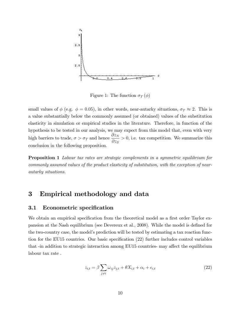
Figure 1: The function σT (φ)

small values of φ (e.g. φ = 0.05), in other words, near-autarky situations, σT ≈ 2. This is

a value substantially below the commonly assumed (or obtained) values of the substitution

elasticity in simulation or empirical studies in the literature. Therefore, in function of the

hypothesis to be tested in our analysis, we may expect from this model that, even with very

high barriers to trade, σ > σT and hence∂zN∂zS

> 0, i.e. tax competition. We summarize this

conclusion in the following proposition.

Proposition 1 Labour tax rates are strategic complements in a symmetric equilibrium for

commonly assumed values of the product elasticity of substitution, with the exception of near-

autarky situations.

3 Empirical methodology and data

3.1 Econometric specification

We obtain an empirical specification from the theoretical model as a first order Taylor ex-

pansion at the Nash equilibrium (see Devereux et al., 2008). While the model is defined for

the two-country case, the model’s prediction will be tested by estimating a tax reaction func-

tion for the EU15 countries. Our basic specification (22) further includes control variables

that -in addition to strategic interaction among EU15 countries- may affect the equilibrium

labour tax rate .

zi,t = β∑j 6=i

ωijzj,t + θXi,t + αi + εi,t (22)

10

where i and j are a country index and t a time index. ωij represent the elements of a weight

matrix ω and Xi,t is a vector of control variables. αi is a fixed effect that captures country

specific time-invariant unobservable determinants such as the Nash equilibrium tax rates or

cross-country differences in the relative preference parameter γ. εi,t is the error term. β and

θ are the parameters to be estimated, together with αi. From the theoretical model, the

hypothesis to be tested is H0 : β ≤ 0, which, in fact, requires a one-sided test.

Based on our reading of the related literature (cf. introduction), we choose the following

variables as elements of Xi,t:

- civil employment;

- the young age dependency ratio;

- the old age dependency ratio;

- the size of the public sector (share of government expenditure in GDP or share of public

in total employment);

- the country share in the OECD GDP (as an indicator of size);

- the country’s GDP per capita;

- the real growth rate of GDP (in purchasing power parities);

- the public debt to GDP ratio;

- the openness rate with respect to the rest of the world (i.e. non-EU15), in terms of

GDP

The public debt to GDP ratio controls for the balanced budget assumption in the model.

The openness rate with respect to non-EU15 countries controls for possible spurious cross-

country correlation between labour tax rates due to common trends in tax policy as a con-

sequence of world economic integration.

Anselin (1988) stresses the crucial importance of a judicious choice of the weighting

scheme for spatially correlated variables because misspecified weight matrices may yield

biased results. Therefore, like Davies and Voget (2008), our weighting scheme of foreign tax

rates builds on the theory that supports the empirical specification. Following the theoretical

model in the previous section the weights are determined by trade freeness, i.e. the distance

between the countries and barriers to trade. As a proxy for the first, we take distances

between major cities. As a simple and exogenous way to account for barriers to trade (or

economic integration) we opt for the number of year of common membership of the EU,

rather than e.g. for trade intensity, which is more subject to endogeneity. With these two

components, we construct four (row normalised) weight matrices with typical elements:

11

ωij,1 =

1dij∑j1dij

; ωij,2 =

(1dij

)2∑

j

(1dij

)2 ;

ωij,3 =

minij(#EUi,#EUj)

dij∑jminij(#EUi,#EUj)

dij

; ωij,4 =

(minij(#EUi,#EUj)

dij

)2∑

j

(minij(#EUi,#EUj)

dij

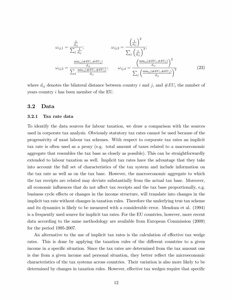
)2 (23)

where dij denotes the bilateral distance between country i and j, and #EUi the number of

years country i has been member of the EU.

3.2 Data

3.2.1 Tax rate data

To identify the data sources for labour taxation, we draw a comparison with the sources

used in corporate tax analysis. Obviously statutory tax rates cannot be used because of the

progressivity of most labour tax schemes. With respect to corporate tax rates an implicit

tax rate is often used as a proxy (e.g. total amount of taxes related to a macroeconomic

aggregate that resembles the tax base as closely as possible). This can be straightforwardly

extended to labour taxation as well. Implicit tax rates have the advantage that they take

into account the full set of characteristics of the tax system and include information on

the tax rate as well as on the tax base. However, the macroeconomic aggregate to which

the tax receipts are related may deviate substantially from the actual tax base. Moreover,

all economic influences that do not affect tax receipts and the tax base proportionally, e.g.

business cycle effects or changes in the income structure, will translate into changes in the

implicit tax rate without changes in taxation rules. Therefore the underlying true tax scheme

and its dynamics is likely to be measured with a considerable error. Mendoza et al. (1994)

is a frequently used source for implicit tax rates. For the EU countries, however, more recent

data according to the same methodology are available from European Commission (2009)

for the period 1995-2007.

An alternative to the use of implicit tax rates is the calculation of effective tax wedge

rates. This is done by applying the taxation rules of the different countries to a given

income in a specific situation. Since the tax rates are determined from the tax amount one

is due from a given income and personal situation, they better reflect the microeconomic

characteristics of the tax systems across countries. Their variation is also more likely to be

determined by changes in taxation rules. However, effective tax wedges require that specific

12

1995 2000 2005 2007Austria 38.5 40.1 40.8 41.0Belgium 43.8 43.9 43.8 42.3Germany 39.4 40.7 38.8 39.0Denmark 40.2 41.0 37.1 37.0Spain 29.0 28.7 30.3 31.6Finland 44.3 44.1 41.5 41.4France 41.2 42.1 41.9 41.3United Kingdom 25.7 25.3 25.5 26.1Greece 38.6 37.8 34.1 33.8Ireland 29.7 28.5 25.4 25.7Italy 38.0 43.7 42.9 44.0the Netherlands 34.6 34.5 31.6 34.3Portugal 26.5 27.0 28.1 30.0Sweden 46.8 47.2 45.0 43.1

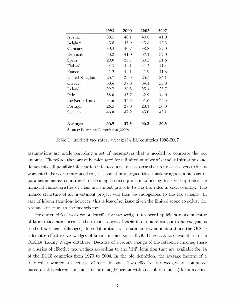
Average 36.9 37.5 36.2 36.5Source: European Commission (2009)

Table 1: Implicit tax rates, averages14 EU countries 1995-2007

assumptions are made regarding a set of parameters that is needed to compute the tax

amount. Therefore, they are only calculated for a limited number of standard situations and

do not take all possible information into account. In this sense their representativeness is not

warranted. For corporate taxation, it is sometimes argued that considering a common set of

parameters across countries is misleading because profit maximising firms will optimise the

financial characteristics of their investment projects to the tax rules in each country. The

finance structure of an investment project will then be endogenous to the tax scheme. In

case of labour taxation, however, this is less of an issue given the limited scope to adjust the

revenue structure to the tax scheme.

For our empirical work we prefer effective tax wedge rates over implicit rates as indicator

of labour tax rates because their main source of variation is more certain to be exogenous

to the tax scheme (changes). In collaboration with national tax administrations the OECD

calculates effective tax wedges of labour income since 1979. These data are available in the

OECDs Taxing Wages database. Because of a recent change of the reference income, there

is a series of effective tax wedges according to the ’old’definition that are available for 14

of the EU15 countries from 1979 to 2004. In the old definition, the average income of a

blue collar worker is taken as reference income. Two effective tax wedges are computed

based on this reference income: i) for a single person without children and ii) for a married

13

wedges

3.pdf

1979 1989 1995 2000 2004Austria 28.5 30.7 34.2 37.2 36.8Belgium 40.3 44.7 48.3 48.4 44.9Germany 35.7 39.7 43.8 42.6 41.5Denmark 35.8 39.5 38.1 37.7 35.7Spain 34.2 33.7 35.9 34.1 34.8Finland 37.0 40.5 46.7 43.6 40.3France 44.3 44.0 43.2United Kingdom 30.6 29.6 29.8 25.8 24.6Greece 17.4 32.9 35.3 36.0 34.9Ireland 27.1 35.3 31.9 22.2 14.9Italy 43.1 47.5 47.6 41.6 41.0the Netherlands 43.7 42.9 39.9 40.3 38.9Portugal 26.2 30.2 30.2 29.9 27.5Sweden 46.6 49.1 45.8 46.0 44.6

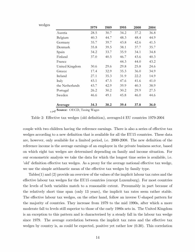
Average 34.3 38.2 39.4 37.8 36.0Source:  OECD, Taxing Wages

Table 2: Effective tax wedges (old definition), averages14 EU countries 1979-2004

couple with two children having the reference earnings. There is also a series of effective tax

wedges according to a new definition that is available for all the EU15 countries. These data

are, however, only available for a limited period, i.e. 2000-2008. The new definition of the

reference income is the average earnings of an employee in the private business sector, based

on which eight tax wedges are determined depending on family and income situation. For

our econometric analysis we take the data for which the longest time series is available, i.e.

’old’definition effective tax wedges. As a proxy for the average national effective tax wedge,

we use the simple arithmetic mean of the effective tax wedges by family type.

Tables(1) and (2) provide an overview of the values of the implicit labour tax rates and the

effective labour tax wedges for the EU15 countries (except Luxemburg). For most countries

the levels of both variables match to a reasonable extent. Presumably in part because of

the relatively short time span (only 13 years), the implicit tax rates seem rather stable.

The effective labour tax wedges, on the other hand, follow an inverse U-shaped pattern for

the majority of countries. They increase from 1979 to the mid 1990s, after which a more

moderate fall to levels still superior to those of the early 1980s sets in. The United Kingdom

is an exception to this pattern and is characterised by a steady fall in the labour tax wedge

since 1979. The average correlation between the implicit tax rates and the effective tax

wedges by country is, as could be expected, positive yet rather low (0.30). This correlation

14

could obviously be biased by the limited number of common years (only 10) for which the

variables are available. Nevertheless the fact that the correlation pattern by country varies

from strongly positive over near zero to strongly negative induces one to question whether

these indicators measure the same underlying variable. Given the possible drawbacks of the

implicit rates discussed above, this strengthens our preference of effective tax wedge rates

over implicit rates as indicator of labour tax rates.

3.2.2 Data of the control variables

Empirical data for most control variables are taken from the following OECD databases: the

National Accounts database (share in the OECD GDP, the GDP per capita and the share

of public expenditure in GDP), the Labour Force Survey database (the activity ratio, the

young and old age dependency ration and the share of public employment) and the Economic

Outlook database (public debt, proxied by the general government gross financial liabilities).

Openness with respect to the rest of the world was determined from the International Trade

by Commodities Statistics database, also from the OECD. The real GDP growth rate was

retrieved from the Penn World Tables.

In the appendix we include the correlation matrix of the independent variables. Overall,

collinearity between the variables is fairly small, except for the old and young age dependency

ratio of which the correlation is -0.78. Given their status as control variables in the empirical

specification, we do not try to correct for this multicollinearity.

3.3 Estimation issues

Spatial interaction effects are typically included in an empirical model at the level of the

explanatory variables (by extending the set of determinants with the spatially lagged de-

pendent variable), at the level of the residual error term, or even at both the level of the

explanatory variables and the error term (the general spatial model). Since the estimation of

the general spatial model in a panel data framework is still in its first stages6, an assumption

has to be made at which level spatial autocorrelation may occur. Given that we derived

our empirical specification in (22) from a theoretical model as a tax reaction function that

includes a spatially lagged dependent variable, we opt for the estimation of a spatial lag

model.

In a panel data framework, the spatial effects are combined with another component of

cross-sectional or spatial heterogeneity, which is typically modelled as a fixed or random

component of the error term, specific for each observation unit. From the theoretical model,

6See Lee and Yu (2010) and Mutl and Pfaffermayer (2008) for recent contributions

15

unobserved country heterogeneity can be linked to differences in inequality aversion (γ) or the

Nash equilibrium tax rate, which are intuitively likely to be fixed components, correlated with

the explanatory variables included in the model. In addition, Elhorst (2009) questions the

appropriateness of the random effects specification in a framework with spatial interaction.

In the commonly considered spatial sample design the population units (i.e. regions, states,

countries,...) are more or less sampled exhaustively and they are not straightforwardly

representative for a larger population. Almost by definition, spatial units are fixed and

inference is conditional on the observed units.

There are two main approaches to estimate a model with spatial correlation: an ap-

proach based on the principle of maximum likelihood (ML) or an instrumental variable (IV)

approach. It is diffi cult to determine the approach that is to be preferred over the other.

Elhorst (2009) mentions that there are indications that the ML-approach of the spatial

lag model (weakly) outperforms the IV-approach, be it in a panel framework without other

sources of cross sectional heterogeneity (random or fixed effects). However, the ML-estimates

may be less consistent than the IV-estimates when the spatial interaction effects are rather

small. In addition, the ML-estimation assumes normality and homoscedasticity of the error

term. Given that we can expect the presence of heteroscedasticity in the error term and

anticipating an at most fairly weak spatial interaction effect, we estimate the model by IV.

Estimating a panel spatial lag model by an instrumental variable approach is a straightfor-

ward extension of the cross-section panel IV-model, using the spatially lagged explanatory

variables as instruments (Anselin et al., 2006). In this approach a heteroscedasticity and

autocorrelation consistent estimate of the error variance-covariance matrix can be obtained

in the lines of White (1980) and Newey and West (1987). This allows to take account of

spatial dependence in the error term in a non-parametric way and can as such constitute an

alternative for a spatial error modellisation (see Anselin, 2006), which, in addition, moder-

ates the consequences of the a priori assignment of the spatial interaction effect to the level

of the explanatory variable, indicated above.

3.4 Results

We estimated equation (22) using effective tax wedges, based on the old reference wage (the

average earnings of a blue collar worker in the manufacturing sector), for the EU15 countries,

with the exception of France and Luxemburg, in the period 1979-2004. Because initially the

effective tax wedges were computed only every two years, we used biennial data for the whole

period. In this way, we obtained a balanced panel of 13 observations in time for 13 countries.

The empirical model was estimated using two sets of instruments for the spatially lagged

16

Variable Coefficient SE Coefficient SE Coefficient SE Coefficient SEW*Y 0.34 ** 0.15 0.16 ** 0.07 0.27 ** 0.13 0.15 ** 0.07Civil employment 0.06 0.11 0.06 0.11 0.06 0.11 0.05 0.11Old age dep.ratio ­0.71 ** 0.30 ­0.73 ** 0.31 ­0.72 ** 0.30 ­0.74 ** 0.31Young age dep. ratio ­0.02 0.17 ­0.03 0.18 ­0.03 0.18 ­0.04 0.18Share public employment 33.84 *** 10.21 34.07 *** 10.15 33.65 *** 10.3 33.75 *** 10.2GDP per capita ­0.49 *** 0.09 ­0.48 *** 0.09 ­0.46 *** 0.09 ­0.47 *** 0.09Share GDP OECD 76.83 52.14 82.1 52.79 75.68 51.85 80.78 51.89Growth rate GDP ­4.61 12.89 ­3.58 13.29 ­5.14 12.86 ­3.96 13.26Public debt ratio 0.14 *** 0.02 0.14 *** 0.02 0.14 *** 0.02 0.14 *** 0.02Openness ROW 23.84 *** 4.87 22.63 *** 4.82 22.6 *** 4.87 22.02 *** 4.84

Number of obs 169 169 169 169Number of countries 13 13 13 13F(10,146) 19.38 *** 19.18 *** 18.95 *** 18.85 ***R² 0.66 0.66 0.66 0.65

Underidentification test   (Kleinbergen­Paap rk LM)

71.35 *** 72.84 *** 70.60 *** 74.21 ***

Weak identification test   (Kleinbergen­Paap rk Wald F)

104.59 *** 113.42 *** 129.25 *** 97.9 ***

Hansen J statistic 9.67 11.5 11.60 12.53

Spatial Weightsωij,1 ωij,2 ωij,3 ωij,4

*, **, and *** indicate significance at the 10%, 5%, and 1% level

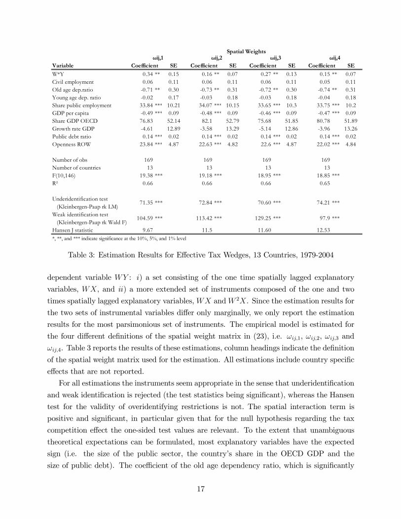
Table 3: Estimation Results for Effective Tax Wedges, 13 Countries, 1979-2004

dependent variable WY : i) a set consisting of the one time spatially lagged explanatory

variables, WX, and ii) a more extended set of instruments composed of the one and two

times spatially lagged explanatory variables,WX andW 2X. Since the estimation results for

the two sets of instrumental variables differ only marginally, we only report the estimation

results for the most parsimonious set of instruments. The empirical model is estimated for

the four different definitions of the spatial weight matrix in (23), i.e. ωij,1, ωij,2, ωij,3 and

ωij,4. Table 3 reports the results of these estimations, column headings indicate the definition

of the spatial weight matrix used for the estimation. All estimations include country specific

effects that are not reported.

For all estimations the instruments seem appropriate in the sense that underidentification

and weak identification is rejected (the test statistics being significant), whereas the Hansen

test for the validity of overidentifying restrictions is not. The spatial interaction term is

positive and significant, in particular given that for the null hypothesis regarding the tax

competition effect the one-sided test values are relevant. To the extent that unambiguous

theoretical expectations can be formulated, most explanatory variables have the expected

sign (i.e. the size of the public sector, the country’s share in the OECD GDP and the

size of public debt). The coeffi cient of the old age dependency ratio, which is significantly

17

Variable Coefficient SEW*Y 0.27 0.40Civil employment 0.04 0.12Old age dep.ratio ­0.67 ** 0.30Young age dep. ratio ­0.03 0.17Share public employment 30.57 *** 10.53GDP per capita ­0.46 *** 0.09Share GDP OECD 74.4 47.96Growth rate GDP ­9.63 12.97Public debt ratio 0.14 *** 0.17Openness ROW 23.60 *** 4.92

Number of obs 169Number of countries 13F(10,146) 19.76 ***R² 0.65

Underidentification test   (Kleinbergen­Paap rk LM)

61.47 ***

Weak identification test   (Kleinbergen­Paap rk Wald F)

53.58 ***

Hansen J statistic 21.66 ****, **, and *** indicate significance at the 10%, 5%, and 1% level

Table 4: Estimation Results for Effective Tax Wedges, Homogenous Weights, 13 Countries,1979-2004

negative, is the most important exception. A similar result is found is some recent estimations

of corporate tax competition (see Devereux et al., 2008, and Davis and Voget, 2010). It

could indicate that countries react to population ageing by lowering the labour tax rate to

encourage people to work.

The positive and significant effect of the spatial interaction term indicates that the labour

tax rates of the considered EU15 countries are strategic complements and suggests the pres-

ence of labour tax competition. From our estimations, the expected direct effect varies

between 0.15 and 0.34, i.e. an average labour tax rate increase of 1 percentage point in the

EU15, induces a single country (directly) to increase its tax rate with 0.2 to 0.3 percentage

points. Hence, though significant and positive, the tax interaction effect does not seem very

strong (which also motivated our choice for IV-estimation rather than ML).

We further explore to what extent we are able to identify the spatial lag mechanism as an

economic integration interaction effect. To this aim we verify if the data are consistent with

an alternative explanation of the spatial lag effect, namely yardstick competition or common

intellectual trends. In line with the literature (see e.g. Devereux et al., 2008), this is done by

re-estimating the model with a spatial weight matrix with uniform elements (ωij =1

(N − 1)).

Table 4 reports the results of the IV-estimation of this model with the effective tax wedges as

18

Variable Coefficient SE Coefficient SE Coefficient SE Coefficient SEW*Y ­0.04 0.11 ­0.02 0.04 ­0.10 0.1 ­0.03 0.04Civil employment 0.37 *** 0.06 0.37 *** 0.05 0.37 *** 0.06 0.37 *** 0.06Old age dep.ratio ­0.90 *** 0.23 ­0.90 ** 0.23 ­0.90 *** 0.23 ­0.90 *** 0.22Young age dep. ratio ­0.47 ** 0.21 ­0.47 ** 0.21 ­0.48 ** 0.22 ­0.48 ** 0.21Share public expenditure 0.01 *** 0.00 0.01 *** 0.00 ­0.01 *** 0.00 0.01 *** 0.00GDP per capita ­0.52 *** 0.09 ­0.52 *** 0.09 ­0.51 *** 0.09 ­0.51 *** 0.09Share GDP OECD ­62.63 *** 19.15 ­61.75 *** 19.58 ­59.15 *** 20.36 ­60.53 *** 20.02Growth rate GDP ­0.01 0.07 ­0.01 0.06 ­0.004 0.07 ­0.01 0.07Public debt ratio 0.02 0.01 0.02 0.01 0.02 0.01 0.02 0.01Openness ROW 11.18 *** 2.54 11.18 *** 2.53 11.22 *** 2.56 11.19 *** 2.53

Number of obs 182 182 182 182Number of countries 14 14 14 14F(10,158) 19.76 *** 19.95 *** 18.95 *** 20.16 ***R² 0.44 0.44 0.43 0.44

Underidentification test   (Kleinbergen­Paap rk LM)

50.72 *** 56.25 *** 48.20 *** 53.41 ***

Weak identification test   (Kleinbergen­Paap rk Wald F)

26.95 *** 66.75 *** 31.71 *** 56.58 ***

Hansen J statistic 5.32 6.04 5.21 7.11*, **, and *** indicate significance at the 10%, 5%, and 1% level

Spatial Weightsωij,1 ωij,2 ωij,3 ωij,4

Table 5: Estimation Results for Implicit Tax Rates, 14 Countries, 1995-2007

dependent variable. Estimation results are very similar to those with bilateral distance (and

number of years of common EU membership) as elements of the weight matrix, except for

the coeffi cient of the spatial lag which is not significantly different from zero. This suggests

that it is unlikely that the observed spatial interaction in labour tax rates can be explained

by common trends or yardstick competition.

In addition to the estimation of (22) using effective tax wedges as data for the labour tax

rates, we estimated the model using implicit tax rates as data for the dependent variable.

With these data a balanced panel was constructed for 14 countries (EU15 less Luxemburg)

and 13 years (the period 1995 to 2007). We report in Table 5 the results of the estimations,

again for the four possible definitions of the weight matrix that we distinguished and using

the same sets of instruments (either WX or the combination of WX and W 2X).

The tests of underidentification and weak identifcation, as well as the test using the overi-

dentifying restriction (Hansen J-test) indicate that the instruments used in these estimations

can be considered as adequate. The coeffi cient estimates vary substantially, however, com-

pared to estimates using effective tax wedges as dependent variable. The spatial interaction

effect turns insignificant, whereas almost all the control variables included are significant,

the public debt to GDP ratio being the surprising exception. Furthermore, except for the

19

public sector size (proxied by the share of public expenditures in GDP), the sign of the

coeffi cients of the significant control variables runs counter to theoretical expectations and

common findings in the literature. All in all, it seems likely that these results for the implicit

tax rate definition suffer from its endogeneity to economic determinants which are unrelated

to the taxation system, economic business cycle effects in particular.

4 Conclusion

In recent years an increasing number of studies has analysed corporate tax competition

between countries, in particular between EU-countries. In this paper we investigate to what

extent tax competition at the national level may also occur for an immobile production

factor, labour in particular.

We derive a tax rate reaction function from a two-country model with transportation

costs in which unemployment is allowed for due to an effi ciency wage mechanism. In our

model a national welfare maximising government is able to redistribute income between the

employed and the unemployed. This is financed by a tax on labour. Bringing the model to

the data, we estimate the labour tax reaction function of EU15-countries and test for the

significance of a positive spatial lag effect. The estimation of a tax reaction function implies

a judicious choice of both the tax rate variable and the weighting scheme for the construction

of the spatially lagged tax rate. As regards the former, our preferred data source is the taxing

wages data of the OECD. As regards the latter, we choose weight matrices with elements

that -in line with the theoretical model- are based on bilateral distance and a simple, but

fairly exogenous indication of economic integration: the number of common years of EU

membership. Our analysis reveals a significant and positive strategic interaction in labour

tax rates. By varying the weighting scheme of the spatial lag matrix, we find no indications

for alternative causal mechanisms, like yardstick competition or common trends. Though

the value of the estimated coeffi cient suggests that the spatial interaction effect is rather

small, we conclude that there are indications that EU-countries take strategic considerations

into account when setting their labour taxes.

20

References

Akerlof, G., Yellen, J., 1986, Effi ciency Wage Models of Labour Market. Cambridge Univer-sity Press, Cambridge.

Altshuler R., Goodspeed T., 2003, Follow the Leader ? Evidence on European and U.S. TaxCompetition, mimeo.

Anselin, L., 1988, Spatial Econometrics: Methods and Models, Kluwer Academic Publishers,Boston.

Anselin, L., 2006, Spatial Econometrics, in: Mills T., Patterson K. (eds.), Palgrave Hand-book of Econometrics. Volume 1: Econometric Theory, 902-958, Palgrave Macmillan,Houndmills Basingstoke.

Anselin, L., Jayet H., Le Gallo J., Spatial Panel Econometrics, in Matyas L, Sevestre P.(eds.), The Econometrics of Panel Data: Fundamentals and Recent Developments inTheory and Practice, 3rd edition, Kluwer, Dordrecht.

Andersen, T.M., 2003, Welfare Policies, Labour Taxation and International Integration,International Tax and Public Finance 10, 43-62.

Bénassy-Quéré A., Gobalraja N., Trannoy A., 2007, Tax and Public Input Competition,Economic Policy, 387-430.

Bretschger L., Hettich F., 2002, Globalisation, capital mobility and tax competition: theoryand evidence for OECD countries, European Journal of Political Economy 18, 695-716.

Brueckner J., 2003, Strategic Interaction Among Governments: An Overview of EmpiricalStudies, International Regional Science Review 26, 175-188.

Casette A., Paty S., 2008, Tax Competition among Eastern and Western European Coun-tries: With Whom Do Countries Compete ?, Economic Systems 32, 307-325.

Davies R., Voget J., 2008, Tax Competition in an Expanding European Union, WorkingPaper 08/30, Oxford Business Centre for Business Taxation, Oxford. Updated versionMarch 2010

Devereux, M., Lockwood B., Redoano M., 2008, Do countries compete over corporate taxrates ? Journal of Public Economics 92, 1210-1235.

Dreher A., 2006, The influence of globalization on taxes and social policy: An empiricalanalysis for OECD countries, European Journal of Political Economy 22, 179-201.

Egger P., Seidel T., 2008, Agglomeration and fair wages, Canadian Journal of Economics,41(1), 271-291.

Elhorst P., 2009, Spatial Panel Data Models, in Fischer M., Getis A. (eds.), Handbook ofApplied Spatial Analysis, 377-407, Springer, Berlin

21

European Commission, 2009, Taxation trends in the European Union. Data for the EU Mem-ber States and Norway, Luxembourg, Offi ce for Offi cial Publications of the EuropeanCommunities.

Garrett G., Mitchell D., 2001, Globalization, government spending and taxation in theOECD, European Journal of Political Research 39, 145-177.

Haufler A., Klemm A., Schjelderup G., 2009, Economic integration and the relationshipbetween profit and wage taxes, Public Choice 138, 423-446.

Helpman E., Grossman G., 2007, Fair Wages and Foreign Sourcing, Working Paper 2008-0045, Weatherhead Center for International Affairs, Harvard University.

Lee L., Yu J., 2010, Estimation of spatial autoregressive panel data models with fixed effects,Journal of Econometrics 154, 165-185.

Kreickemeier U., Nelson D., 2006, Fair wages, unemployment and technological change in aglobal economy, Journal of International Economics, 70, 451-469.

Martin P., Rogers C.A., 1995. Industrial Location and Public Infrastructure, Journal ofInternational Economics 39, 335-357.

Newey W., West K., 1987, A Simple, Positive Semi-Definite Heteroskedasticity and Auto-correlation Consistent Covariance Matrix, Econometrica 55, 703-708.

Mendoza E., Razin A., Tesar L., 1994, Effective tax rates in macroeconomics: cross-countryestimates of tax rates on factor incomes and consumption, Journal of Monetary Eco-nomics 34, 297-323.

Mutl J., Pfaffermayr M., 2008, The Spatial Random Effects and the Spatial fixed EffectsModel: The Hausman Test in a Cliffand Ord Panel Model, Working Paper, 229, Institutefor Advanced Studies, Vienna.

Rayp G., Vanbergen B., 2008, Are Social Welfare States Facing a Race to the Bottom ?A Theoretical Perspective, Working Paper 08/572, Faculty of Economics and BusinessAdministration, Ghent University.

Redoano M., 2007, Fiscal Interactions Among European Countries. Does the EU Matter ?,CESIfo Working Paper 1952, CESIfo.

Rodrik D., 1997, Trade, Social Insurance, and the Limits to Globalization, Working Paper5905, NBER.

Stiglitz, J.E., 1976. The effi ciency wage hypothesis, Surplus Labour and the Distribution ofIncome in L.D.C.’s., Oxford Economic Papers, 28, 185-207.

Summers, L.H., 1988, Effi ciency Wages, Labour Relations and Keynesian Unemployment,American Economic Review 78(2), 383-388

22

White H., 1980, A Heteroskedasticity-Consistent Covariance Matrix Estimator and a DirectTest for Heteroskedasticity, Econometrica 48, 817-838

Wilson, J., Wildasin, D., 2004. Capital Tax Competition: Bane or Boon, Journal of PublicEconomics, 88(6), 1065-1091.

23

Appendix

Civil Youg age Old age Share GDP Share GDP Growth rate Public debtemployment depency ratio depency ratio public employment  per capita  OECD GDP ratio

Young age dep ratio 0.375Old age dep ratio ­0.196 ­0.779Share public employment 0.568 0.423 ­0.274GDP per capita ­0.066 0.296 ­0.358 ­0.053Share GDP OECD 0.387 0.496 ­0.553 0.612 0.128Growth rate GDP ­0.081 ­0.212 0.131 ­0.011 ­0.162 ­0.022Public debt ratio ­0.353 0.182 ­0.145 0.208 ­0.150 0.156 0.159Openess ROW 0.008 ­0.312 0.253 0.341 ­0.147 0.348 0.276 0.214

Table 6: Correlation matrix

24