CLASSIFICATION NOTES NO. 30.4 DET NORSKE VERITAS FOUNDATIONS FEBRUARY 1992 Det Norske Veritas Classification AS VERITASVEIEN 1, N-1322 H0VIK, NORWAY TEL: +47 67 57 99 00 FAX: +47 67 57 99 11

DNV CN 30.4 Foundations
Oct 27, 2014
Welcome message from author
This document is posted to help you gain knowledge. Please leave a comment to let me know what you think about it! Share it to your friends and learn new things together.
Transcript
CLASSIFICATION NOTES NO. 30.4
DET NORSKE VERITAS
FOUNDATIONS
FEBRUARY 1992
Det Norske Veritas Classification AS V E R I T A S V E I E N 1, N - 1 3 2 2 H 0 V I K , N O R W A Y T E L : +47 67 57 9 9 00 F A X : +47 67 57 99 11
FOREWORD
Det norske Veritas is an independent Foundation with the objective of safeguarding life, property and the environ-ment at sea and ashore. Classification, certification and quality assurance of ships, offshore installations and industrial plants, as well as testing and certification of materials and components, are main activities.
Det norske Veritas possesses technological capability in a wide range of fields, backed by extensive research and development efforts. The organization is represented world-wide in more than 100 countries.
Classification Notes are publications which give practical information on classification of ships, offshore installa-tions and other objects. Examples of design solutions, calculation methods, specifications of test procedures, quality assurance and quality control systems as well as acceptable repair methods for some components are given as interpretations of the more general rule requirements. An updated list of Classification Notes available is given in the latest edition of the Introduction-booklets to the «Rules for Classification of Steel Ships», «Rules for Classification of Mobile Offshore Units» and «Rules for Classification of Fixed Offshore Installations)).
© Det norske Veritas 1992 Computer Typesetting by Division Ship and Offshore, Det norske Veritas Classification A/S Printed in Norway by Det norske Veritas
02.92.2000
It is agreed that save as provided below Det norske Veritas, its subsidiaries, bodies, officers, directors, employees and agents shall have no liability for any loss, damage or expense allegedly caused directly or indirectly by their mistake or negligence, breach of warranty, or any other act, omission or error by them, including gross negligence or wilful misconduct by any such person with the exception of gross negligence or wilful misconduct by the governing bodies or senior executive officers of Det norske Veritas. This applies regardless of whether the loss, damage or expense has affected anyone with whom Det norske Veritas has a contract or a third party who has acted or relied on decisions made or information given by or on behalf of Det norske Veritas. • However, if any person uses the services of Det norske Veritas or its subsidiaries or relies on any decision made or information given by or on behalf of them and in consequence suffers a loss, damage or expense proved to be due to their negligence, omission or default, then Det norske Veritas will pay by way of compensation to such person a sum representing his proved loss. * In the event Det norske Veritas or its subsidiaries may be held liable in accordance with the sections above, the amount of compensation shall under no circumstances exceed the amount of the fee, if any, charged for that particular service, decision, advice or information. * Under no circumstances whatsoever shall the individual or individuals who have personally caused the loss, damage or expense be held liable. * In the event that any provision in this section shall be invalid under the law of any jurisdiction, the validity of the remaining provisions shad not in any way be affected.
CONTENTS
1. SOIL INVESTIGATIONS FOR FIXED OFFSHORE STRUCTURES 4
1.1 Introduction 4 1.2 Methods and techniques 4 1.3 Soil investigation for gravity type foundations . 7 1.4 Soil investigation for pile foundations 8 1.5 Soil investigation for jack-up platforms 8 1.6 Soil investigation for pipelines 9
2. AXIAL PILE RESISTANCE 10 2.1 Introduction 10 2.2 Resistance in cohesive soils 10 2.3 Resistance in cohesionless soils 13 2.4 Resistance in calcareous soils 15 2.5 Group effects 15 2.6 Effects of installation procedure 15 2.7 Effects of cyclic loading 15
3. LATERAL PILE RESISTANCE 16 3.1 Introduction 16 3.2 Piles in cohesive soils 16 3.3 Piles in cohesionless soils 18 3.4 Piles in calcareous soils 19 3.5 Modifications of p—y curves 19 3.6 Plastic analysis of piles 20
4. STABILITY OF GRAVITY BASE FOUNDATIONS 20
4.1 Introduction 20 4.2 Soil shear strength 21 4.3 Solution methods 26 4.4 Bearing capacity formulae 28
5. SETTLEMENT OF GRAVITY FOUNDATIONS 31
5.1 Introduction 31 5.2 Stress distribution theories 32 5.3 Settlement calculations 36 5.4 Time rate of consolidation 38
6. PENETRATION RESISTANCE OF SKIRTS 39 6.1 Introduction 39 6.2 Methods of calculation 40
7. SOIL-STRUCTURE INTERACTION 41 7.1 Introduction 41 7.2 Global dynamic foundation stiffness for GBS
type foundation 41 7.3 Soil reaction on structural foundation elements 43
8. FOUNDATION OF JACK-UP PLATFORMS 44 8.1 Introduction 44 8.2 Individual leg supported jack-up platforms . . . 45 8.3 Mat-supported jack-up platforms 49 8.4 Foundation restraints 50
9. REFERENCES 52
4 Classification Notes — No. 30.4
1. Soil Investigations for Fixed Offshore Structures 1.1 Introduction 1.1.1 General 1.1.1.1 Guidelines for determination of soil investi-gation programme for gravity type foundations, piled foundations and foundations of pipelines are given in this Chapter. Brief descriptions of the various methods and techniques to be used in geophysical and geotechnical surveys are given.
1.1.2 Planning
1.1.2.1 The required amount of information with re-spect to soil properties normally changes during a field development. At an early stage the gathered data should be sufficiently detailed to demonstrate the feasibility of a given concept. Also, the information available at this stage facilitates the selection of the most favourable lo-cation for the structure within the development area. At a final stage the soil investigation should provide all nec-essary data for a detailed design of a specific structure at the specific location.
1.1.2.2 The soil investigation necessary for field devel-opment should normally be performed in progressive stages so that structural concepts can be developed with due regard to soil conditions. In order to optimize the extent of the soil investigation, planning should be done based on the results from previous findings. Factors as geological history, uniformity*of foundation deposits, size and type of structure etc. should be reflected in the extent of the site investigation.
1.1.2.3 The sequence of the soil investigation for a platform should be as follows:
• Collection of available geological, geotechnical and foundation performance data for the area.
• Carrying out of a geophysical survey at an early stage of the field development, comprising: - Bathymetry and seabed surveys - Sub-bottom profiling. This is to be supplemented with a feu seabed samples (e.g. gravity cores) and one or two soil borings.
• When the type and location of platform have been determined, a detailed geotechnical investigation and topographical mapping and seabed survey of the ac-tual location should be carried out.
1.2 Methods and techniques
1.2.1 General 1.2.1.1 The soil investigations may be divided in:
• Geological studies • Geophysical surveys • Geotechnical investigations.
Below, brief descriptions of the various survey methods and techniques are given. General sampling recommen-
dations and guidelines for planning of laboratory test programmes are also presented.
1.2.2 Geological studies
1.2.2.1 The geological study should be based on infor-mation about the geological history of the general area of field development. The purpose of such a study is to establish a basis for selection of methods and extent of the site investigation.
1.2.3 Geophysical surveys
1.2.3.1 The main purpose of the geophysical survey should be to extend the more localized information from borings and in situ testing to get an understanding of the seabed topography and the stratification within defined areas. As such, these surveys should give guidelines in se-lection of suitable platform sites within the exploration area.
1.2.3.2 Seabed topography and layering are investigated by means of seismic methods. Geophysical surveys are carried out by towed devices with specifed characteristics.
1.2.3.3 For determination of water depth and sea floor topography, high accuracy echosounders may be used together with vessel movement sensors (surface system). However, use of a towed fish with echosounder and pressure sensor will improve the accuracy significantly. By adding a side-scan sonar device to the towed system, any seabed obstruction or feature may be investigated in more detail by towing closer to the seabed. Manned or unmanned submersibles for visual/video surveys of the actual foundation area will complement the echosounder and sonar profiles. Echosounders with adequate high fre-quency response may detect gas seeps at the sea floor and particularly soft seabed deposits. Steel and iron objects may be detected with a marine proton magnetometer bottle, which measures the total magnetic field intensity along the tow line. Obstacles detected at the sea bottom shall be carefully mapped and identified.
1.2.3.4 The choice of an appropriate geophysical pro-filing system depends upon the required depth of pene-tration, the desired degree of resolution and the seismic response of the shallow formations. The resolution, i.e. the ability to identify the different sub-bottom layers, in-creases as the frequency of the transmitted and received signals increases. However, higher frequencies result in larger absorption losses in the ground and less pene-tration. The basic components of a seismic profiling sys-tem are a sound source, hydrophones and a recording unit. Typical operating characteristics for high energy systems are frequencies in the range 100—400Hz capable of achieving penetrations down to about 300m depth with a resolution of some metres. A high resolution profiling system should contain a set of towed devices having dif-ferent frequency response. The necessary depth to which the investigation should extend depends on the geological formations and the type of structure.
1.2.3.5 Coarse grid surveys may give guidelines in se-lecting the optimum foundation site where detailed sur-veys must be done. By reducing the grid spacing, details of the geologic formations may be obtained for the most interesting area.
Classification Notes — No. 30.4 5
1.2.4 Geotechnical surveys in general
1.2.4.1 The principal methods to be employed in a geo-technical investigation are:
• Sampling for laboratory testing • In-situ testing.
The geotechnical investigation at the actual platform site should secure all data necessary for the foundation de-sign. Options for modifications of the initial site investi-gation program in the course of the survey may be favourable. A qualified geotechnical engineer should therefore be onboard the survey vessel. The soil investi-gation should be tailored to the design methods used. To facilitate the interpretation of the test results, an overlap of information between the various methods em-ployed should be planned. The field and laboratory in-vestigations should establish the detailed soil stratigraphy across the site providing the following types of geotech-nical data for all important layers:
• Data for classification and description of the soil • Parameters required for a detailed and complete foun-
dation design.
1.2.5 Sampling without drilling
1.2.5.1 Grab samplers, gravity corers and bottom oper-ated corers may secure soil samples from the top soil layers. With present equipment these samples have usu-ally been found disturbed and consequently only useful for identification purposes.
1.2.5.2 Gravity corers consist essentially of a heavy torpedo-shaped body with a sampling tube (50—100 mm diameter) attached in front. The basic method of opera-tion is to lower the corer on a wire until it is a few metres above the sea bottom. It is then released and allowed to fall to the bottom. In soft to firm clays the depth of pen-etration is 3—5m while no penetration may be experienced in dense or hard soils.
1.2.5.3 Piston corers look like gravity corers but take longer samples. The piston remains near the top of the sediment by sliding up the sampling tube as the corer penetrates into the seabed. By this method samples ex-ceeding 40m in length have been taken. The tube diameter is 50-100 mm.
1.2.5.4 Vibratory sampling can provide soil samples up to 8m in length in soft to firm clays and loose sands while the length may be limited to 0.5—2m in hard clays. The sampling is carried out from a rig, lowered to the seabed and remotely controlled from the surface. The sampling tube has a diameter of 100—270 mm.
1.2.6 Sampling from a drilled borehole
1.2.6.1 For sampling at greater depths drilling of a bo-rehole is recommended. The sampling device is then low-ered inside the drillstring to the bottom of the borehole at the depth where a sample is taken. The boring is made with a straight flush rotary drilling technique. Drilling mud may be needed to remove the cuttings and to stabi-lize the hole. The top of the drillstring is connected to a motion compensator in the crown of the derrick so that the drillstring is in constant tension. The maximum
available bit pressure is governed by the weight of the drill collars and the tension force required to avoid buckling of the drillstring above mudline.
1.2.6.2 The traditional sampling method is percussion sampling with a wireline tool consisting of a thin-walled tube and a sliding hammer. The percussive action of the falling weight produces clay samples which are signif-icantly disturbed.
1.2.6.3 The sample disturbance is reduced to some ex-tent by push sampling. Different techniques have been developed for this type of sampling:
a) The sample tube is latched into the drillstring and pushed into the soil by the weight of the drillstring (by reducing the tension load).
b) The sample tube is pressed into the soil by hydraulic jacks operating: • either from the sea floor as part of a heavy jacking
unit providing the reaction force • or within the drillstring near the bit with the re-
action force provided by friction between the bore-hole wall and inflatable packers inserted in the drillstring just above the bit.
Wherever possible push sampling should be preferred as compared to percussion sampling, especially in cohesive soils.
1.2.6.4 Rotary sampling tools are generally used for drilling and sampling in hard formations such as rock cemented sand, hard heavily-overconsolidated clays, and boulder type clays. A typical tool of this type is the ma-rine wireline double walled core barrel. Cores are taken by rotating outer barrel, while the non-rotating inner barrel is stationary around the core. After coring is com-pleted the inner tube and the core are recovered to the surface by use of the wireline assembly.
1.2.7 General sampling requirements
1.2.7.1 The sampling tools should be checked for proper operation and should be equipped with undamaged, properly machined sample retainers. Where sampling is carried out from the bottom or a borehole, care must be taken to achieve a clean borehole free from cuttings and debris at the time of sampling. If metallic tubes are used to secure and store «undisturbed» samples, only new tubes with proper cutting edge should be employed. The sampling operation should be conducted in such a way that damage to the sampler and disturbance of the soil samples are avoided.
1.2.8 In-situ testing
1.2.8.1 The cone penetrometer test (CPT) is the most commonly used in-situ testing method in offshore soil in-vestigations. The test is carried out either from an un-derwater rig without drilling of a borehole (e.g. «Seacalf»), from a seafloor-based jacking unit (e.g. «Stingray») or down-the-hole without use of any seafloor unit (e.g. «Wison»). The test is carried out by pushing a 10cm2 cone at a pen-etration rate of 2cm/s into the soil. The cone tip simul-taneously measures the tip (cone) resistance and the
6 Classification Notes — No. 30.4
friction along a sleeve behind the tip. The results provide useful information, both quantitatively and qualitatively about soil strength and stress-strain characteristics. Piezo cone penetrometers, which incorporate also a pressure transducer at the tip to measure the pore pressure, are the most common today in offshore site investigations.
1.2.8.2 The «Seacalf» rig or similar equipment performs remotely controlled static cone penetrometer tests from the seabed using a hydraulic jacking system and a re-action force of 60—260 kN provided by the ballasted frame of the rig. The depth of penetration typically ranges from about 20m in hard clays or dense sands to 30—60m in soft normally consolidated clays. Continuous plots of cone resistance, sleeve friction and excess pore pressure as function of depth may be obtained.
1.2.8.3 The «Stingray» rig or similar equipment is an ocean floor, hydraulically powered drillstring reaction device typically weighing 230 kN. Sampling or in-situ testing can be performed on the seafloor or at any depth. It is designed to operate in water depths down to 900m. Cone testing is carried out in increments of max. 3—6m or until refusal. After each increment the cone is re-trieved by use of the wireline and the drillpipe is advanced to the depth penetrated by the cone. At this depth the cone penetrometer testing is resumed. This procedure is repeated until the complete depth of interest is tested. The «Stingray» is designed to accommodate cone penetrome-ter tests, vane tests, pressure-meter tests, load tests as well as soil sampling.
1.2.8.4 The «Wison» cone penetrometer system enables in-situ tests to be performed from the base of a borehole. The cone penetrometer is lowered inside the drillstring and latches to the drillcollar. The Wison is activated to push the penetrometer into the soil. After reaching maxi-mum depth (about 3m) or earlier if the total thrust ca-pacity is reached, the tool is depressurized. The drillstring is lifted to retract the test rod and the Wison unit subse-quently retrieved. Also the «Wison» CPT, with or without measurement of pore pressure, can be carried out in combination with wireline sampling or push sampling.
1.2.8.5 The Remote Vane is a wireline tool to be used for in-situ measurement of the soil's undrained shear strength. The instrument has two main sections — the tool body and the motion compensating section. The lower portion of the tool body contains the test vane and a reaction vane, both of which are inserted into the soil. The operational sequence for performing a Remote Vane test begins by advancing the borehole to a depth approx-imately lm above the desired test depth and then sus-pending the drillpipe with the drill bit a couple of metres above the bottom of the hole. The tool is then lowered through the drillpipe until it rests on the bottom of the borehole, and the motion compensating unit is approxi-mately 80% retracted. While the tool rests on the bottom with its weight removed from the wireline, the pawls are activated to extend from the tool body. The drillpipe is then lowered until the open-center drill bit bears on the pawls, pushing the vane blade to the desired test depth. The drillpipe is again suspended off bottom and the test is performed. After the test is completed, the tool is re-trieved and the borehole is advanced to the next depth.
1.2.8.6 The pressuremeter is a dilatable cylindrical probe which is generally run into a borehole or sometimes driven into the soil. The test at a given depth consists of measuring the pressure-volume relationship during the dilation phase. Any pressuremeter test includes two suc-cessive operations, i.e. setting the probe in place and then expanding the cell together with data acquisition. This is a process capable of determining the static as well as the dynamic stress-strain characteristics of the soil.
1.2.8.7 Radioactive well logging is carried out by low-ering into a borehole a probe containing radioactive iso-topes. On its way down through the drillstring a recording is done on a paper trace which will give the wet density and/or the moisture content profile through the surveyed depth. The «gamma radiation method» uses a source of gamma rays inserted at a fixed distance from a Geiger type gamma ray detector. The induced gamma rays pass into the soil and the detector records the number of rays which undergo Compton scattering which is a measure of the wet density of the soil. This probe contains a source of high energy neutrons which pass into the surrounding soil and are reduced in energy especially by colliding with hydrogen nuclei. By providing a unit which detects low energy neutrons, a measure is obtained of the moisture concentration.
1.2.8.8 The measurement of in-situ shear wave velocity requires a system comprising a source generating shear waves, receivers, preferably 3-component. a recorder to measure travel times and a triggering system for trigger-ing the recorder. The source may be located either at the seabed with the receivers at different depths below the seabed or in one of two parallel boreholes with the re-ceivers in the other borehole. The former of these tech-niques is the most common for offshore applications. The receivers are located in a cone penetrometer unit which can be lowered by wireline and latched into the bottom of the drillstring. By this device the shear wave velocity can be measured as a function of depth. In a second step the small strain shear modulus (Gmax) of the soil can be calculated. The simultaneous measurement of the cone resistance makes this so-called «seismic cone» a very useful tool.
1.2.8.9 The dilatometer consists of a flat blade which is pushed into the undisturbed soil from the bottom of a borehole or from the seabed. For the offshore dilatome-ter, which is smaller than the onshore Marchetti device to fit inside the standard drillpipe used offshore, oil pres-sure is used to expand the membrane. Readings are taken of the membrane «lift off» pressure (at rest pressure, p0) and the 1-mm expansion pressure (pi). A filter located on the opposite side of the membrane centre allows pore pressure to be measured continuously. The dilatometer can be used to determine the lateral earth pressure in-situ and thus the earth pressure coefficient K(>. Tentative em-pirical relationships are also developed for derivation of other geotechnical design parameters.
1.2.8.10 As a guidance for assessment of a minimum setting depth of conductors, so-called «hydraulic fracture testing» is used. Equipment and procedures for this type of testing are still under development based on practical experience from various prototype testing in connection with offshore soil investigations.
Classification Notes — No. 30.4 7
1.2.9 Laboratory investigations 1.2.9.1 The recovered soil samples should be described both onboard and later in the onshore laboratory. The description should comprise estimates of:
• Grain size distribution • Colour and smell • Consistency • Laminations • Carbonatic reaction • Other relevant information.
1.2.9.2 The samples should be properly cleaned, marked, sealed and stored. Storage, handling and trans-portation of the samples should be as gentle as possible to avoid or limit disturbance.
1.2.9.3 The onboard laboratory testing should normally comprise the following determinations:
• Water content • Unit weight • Undrained shear strength of cohesive samples by me-
ans of pocket penetrometer, torvane, miniature vane, fall cone and UU triaxial test
• Carbonatic reaction • Grain size distribution of selected cohesionless samples • Liquid and plastic limits of selected cohesive samples.
Recently even more advanced laboratory tests, e.g. oe-dometer tests, direct simple shear tests etc. have been performed with success onboard the vessel. An experienced geotechnical engineer or an engineering geologist should be present on board during sampling and laboratory testing.
1.2.9.4 The onshore laboratory testing should be carried out on representative samples which shall as closely as possible be subjected to the same stress conditions as ex-perienced offshore. It is essential that initial stress condi-tions, overconsolidation ratio and stresses induced by the structure and environment are realistically reflected. A combined static/cyclic test programme should allow de-termination of stiffness, damping and strength of the soil under the range of load conditions to be covered by the design. The random nature of wave and earthquake loading re-quires that special attention should be paid to the load simulation technique used in the testing. The chosen procedure should reflect the effect of the stress level and load duration on the development of pore pressure and shear strain. The types of tests which should normally be considered in the planning of a programme are the following:
• Classification and index tests such as: - Unit weight of sample - Unit weight of solid particle - Water content - Liquid and plastic limits - Grain size distribution - Salinity - Carbonate content.
• Permeability tests. • Consolidation tests. • Static tests for determination of shear strength pa-
rameters: - Triaxial tests (UU, ClUa, CAUa, CAUp, oedo-
triax, Kq) - Direct simple shear (CCV).
• Test for determination of remoulded shear strength (type UU, CIU).
• Cyclic tests for determination of strength and stiffness parameters: - Triaxial tests (CIUc, CAUc) - Direct simple shear (CCVc) - Resonant column (ClUrc) - Shear wave velocity measurement.
1.3 Soil investigation for gravity type foundations
1.3.1 General
1.3.1.1 The soil investigation for a gravity type founda-tion should give basis for a complete foundation design comprising evaluations of:
• Stability • Settlements • Penetration and retrieval resistance of skirts • Local contact stresses • Dynamic response of foundation soil.
1.3.2 Geophysical surveys
1.3.2.1 The minimum depth of sub-bottom profiling should correspond to the depth to rock or the width of the largest base dimension. The required accuracy for sea bed topography measurements is normally in the order of ±0.1—0.2m for relative elevations. This is outside the capacity of echosounders operated from the sea surface subject to wave and wind effects. Alternative methods include submarines or remotely controlled underwater vehicles equipped with differential pressure transducers or echosounders. Any obstructions e.g. large boulders discovered during seismic and topographic surveys within the foundation area should be accurately located. A fairly close grid of seismic profiles (50—100m spacing) over the actual area for correlation with other investigation results will reduce the number of borings to a minimum.
1.3.3 Geotechnical surveys
1.3.3.1 As basis for all foundation analyses an extensive investigation of the shallow soil deposits should be per-formed. The minimum depth should be deeper than any possible critical shear surface. Further, all soil layers in-fluenced by the structure from a settlement point of view should be thoroughly investigated.
1.3.3.2 The extent of shallow borings with sampling should be determined based on type and site of structure as well as on general knowledge about the soil conditions in the area of platform installation. Emphasis should be given to the upper layers and potentially weaker layers
8 Classification Notes — No. 30.4
further down. Sampling intervals should not exceed 1.0—1.5m. A number of seabed samples (gravity cores or equivalent) evenly distributed over the area should also be taken for evaluation of scour potential.
1.3.3.3 In addition to the borings, shallow CPTs dis-tributed across the installation area should be carried out. The number of CPTs depends on size and type of struc-ture and soil conditions. If the soil conditions are very irregular across the foundation site, the number of CPTs will have to be increased. The shallow CPTs should give continuous graphs from mudline to the maximum depth of interest.
1.3.3.4 For settlement evaluations and determination of dynamic response of the foundation soil, investigation of the soil to a greater depth is necessary. The depth should not be less than that corresponding to the largest base dimension of the structure. The investigation should consist of one boring with continuous CPT and at least one boring with sampling close to the CPT hole. The sampling interval is to be determined from the CPT re-sults but should not exceed 3m.
1.3.3.5 If, during the course of the soil investigation, a weaker layer is encountered, along which a critical failure surface can be expected, special emphasis should be put on investigation of this layer.
1.3.3.6 Special tests such as plate loading tests, pressu-remeter tests and shear wave velocity measurements should be added where relevant.
1.4 Soil investigation for pile foundations
1.4.1 General
1.4.1.1 The soil investigation for a pile foundation should give basis for a complete foundation design com-prising evaluations of:
• On-bottom stability of unpiled structure • Lateral pile capacity • Axial pile capacity • Pile drivability predictions.
1.4.1.2 The extent of the soil investigation is dependent on type and size of the structure and the consistency and degree of uniformity of the foundation soil.
1.4.2 Geophysical surveys
1.4.2.1 In 1.2.3 the demands to a geophysical survey are described. As for gravity foundations it is essential to carry out a coarse grid geophysical survey at an early stage of the field development. The minimum depth of seismic profiles should be the anticipated depth of pile penetration plus a zone of influence of about ten pile di-ameters.
1.4.2.2 A topographic survey of the selected area should be carried out. Remotely controlled underwater vehicles with video camera and differential pressure transducers will provide data of sufficient accuracy. Any obstructions, within the foundation area, discovered during the seabed surveys shall be accurately mapped.
1.4.3 Geotechnical surveys
1.4.3.1 For on-bottom stability and lateral pile analyses shallow cone penetration tests should be carried out from mudline to 20—30m depth. In addition, shallow borings with sampling should be performed for better determi-nation of characteristics of the individual layers identified by the cone penetration tests. The sampling interval should not exceed 1.0—1.5m.
1.4.3.2 A number of seabed samples (gravity cores or equivalent) evenly distributed over the area should be taken for evaluation of scour potential.
1.4.3.3 For axial pile capacity analysis at least one down-the-hole CPT boring giving a continuous CPT profile and one nearby boring with sampling should be carried out. The minimum depth should be the antic-ipated penetration of the pile plus a zone of influence. The zone of influence should be sufficient for evaluation of the risk of punch through failure. The sampling inter-val should be determined from the CPT results but should not exceed 3m.
1.4.3.4 If no potential end bearing layers or other dense layers which may create driving problems are found, the above scope of sampling and in-situ testing are sufficient.
1.4.3.5 In case potential end bearing layers or other dense layers are found, additional cone penetration test-ing and sampling should be carried out in order to deter-mine the thickness and lateral extension of such layers within the foundation area. Use of rotary sampling tools may be recommended in very hard or dense formations.
1.5 Soil investigation for jack-up platforms
1.5.1 General
1.5.1.1 For general site assessment and evaluation of the foundation behaviour of a jack-up rig, adequate geotech-nical and geophysical information should be available, including information about:
• Seafloor topography and sea bottom features. • Soil stratification and classification. • Characteristics for soil in various strata.
1.5.1.2 The most important soil parameters are the soil shear strength parameters, i.e. undrained shear strength or the effective stress parameters cohesion (alternatively attraction) and angle of internal friction. As found rele-vant in each case, it may also be required to determine other characteristics such as grain size distribution, rela-tive density, unit weight and in-situ small strain shear stiffness Gmax-
1.5.1.3 The soil investigations may be based on a com-bination of the following types of information:
• General geological knowledge about the area • Geophysical investigations (bathymetry, sidescan so-
nar, shallow seismic) • Sampling and laboratory testing • In situ testing, e.g. cone penetration test.
Classification Notes — No. 30.4 9
1.5.2 Geophysical surveys
1.5.2.1 Geophysical investigations required for a site assessment includes bathymetric survey, seabed surveys with side scan sonar or high resolution multibeam echo-sounder and shallow seismic surveys. The various surveys are normally performed in parallel from one survey vessel using multipurpose tow equipment. Shallow seismic with digital recording will have to be performed separately, however. At the selected location, the line spacing should be suffi-ciently small to detect all features of interest, such as seabed irregularities or debrises, variations in subsoil strata including erosion channels etc. Interlining within the area of most interest may be decided based on initial survey of a wider area with coarser spacing. Depending on the general irregularities detected by the first survey, the line spacing for the detailed central survey can be decided. Typical spacings may be 100 x 250m for a coarse grid ana 25 x 50m for a finer grid.
1.5.2.2 The purpose of the seabed survey is to detect seabed irregularities or debrises, as reefs, iceberg plough-marks, pockmarks, wrecks or other debrises. For de-tection of pipelines, cables or other metallic debris at or slightly below the seabed, magnetometer surveys may be required.
1.5.2.3 The purpose of shallow seismic surveys is to de-termine the soil stratigraphy to a depth of interest as in-dicated in 1.5.3.4 and to detect any possible presence of shallow gas concentrations. The determination of soil stratigraphy requires correlation with soil boring data within the surveyed area. Even when a boring is per-formed at the location, a shallow seismic survey should be available to be able to show whether irregularities exist within the foundation area that give other foundation conditions than that determined by the boring, e.g. detect possible erosion channels or general variations in layer thicknesses of importance.
Analog records may be used for determination of soil stratigraphy whereas registration of shallow gas will re-quire digital recording. The equipment characteristics (energy and frequency) should be chosen to fit the ex-pected soil conditions and the correspondingly required depth for determination of soil stratification.
1.5.3 Geotechnical surveys
1.5.3.1 The required extent of the geotechnical surveys is dependent on the variability of the soil conditions in the area, and on possible problems foreseen for the subject jack-up platform at the given location. In the planning for site specific soil investigations, any existing information should be made available, such as general geological knowledge about the area, results from possible previous geophysical investigations, borings and/or in situ testing.
1.5.3.2 As a minimum at each platform location, one should normally provide either one borehole with sampl-ing and laboratory testing, or carry out in-situ testing. Such testing can be omitted provided that:
1) Existing knowledge about the general geology of the area (history of deposits) together with geophysical
surveying can justify extrapolation from documented soil profiles nearby the platform location.
2) It can be documented that, based on a possible range of soil conditions derived from existing soil data, the platform can be safely operated during installation (preload) as well as during normal operations and pull-out phases, see Chapter 8.
1.5.3.3 If the area, within which the platform is to be located shows irregular soil conditions, it may be neces-sary to perform more than one boring/ in-situ testing in order to verify the variations within the foundation area. For such events the uncertainties in positioning should be considered. Special concern should be given to the possibility of bur-ied erosion channels with soft infill material.
1.5.3.4 The design shear strength profile should be es-tablished to a depth below which the soil conditions have no influence on the foundation behaviour. For platforms supported by individual leg foundations (spud cans) the required depth of the documented soil profile will nor-mally be one to two spud-can diameters below the antic-ipated penetration of the spud can. For mat supported foundations, usually only the upper few metres are of in-terest, except at locations with very soft clays where a deepseated failure may be relevant to study, see 8.3.1.4.
1.5.3.5 In areas with high potential of scour, grain size distribution tests should be performed on samples from the upper 2—3m in order to improve evaluations of scour potential.
1.6 Soil investigation for pipelines 1.6.1 General
1.6.1.1 The site investigation for a pipeline typically consists of a shallow seismic profiling survey of the wide lay barge anchoring corridor, a detailed bathymetric sur-vey of the 100—150m wide construction corridor and fi-nally a geotechnical investigation comprising cone penetration tests (CPT), push sampling, vibro coring, gravity coring etc. To define the various soil deposits along a proposed pipeline route, the emphasis is put on the shallow seismic profiling results. In-situ testing and sampling should subsequently be performed for determi-nation of the soil properties in these deposits.
1.6.2 Geophysical surveys
1.6.2.1 Total water depth is needed to determine ex-ternal water pressure on the pipe and wave effects on the bottom sediments. The trenching, laying and burying methods will also be dependent on water depth. The seabed topography will influence the support conditions of the pipe, the formation of free spans and the stability of the seabed itself. Consequently, surveys with precise echosounders and sidescan sonar are usually required. The accuracy of such measurements will directly influence the degree of conservatism in the design of the pipeline itself.
1.6.2.2 Especially in areas of highly variable seabed to-pography, the limitations of the echosounder may neces-sitate more accurate mapping methods. Profiling with
10 Classification Notes — No. 30.4
small submarines may improve the accuracy compared with that of surface vessels. Seismic profiling is necessary to define the extent and variations of the various soil deposits along the pipeline route. The equipment used should give good resolution for the shallow layers down to about 10m depth for definition of erodable materials, applicability of trenching methods and stability of the pipeline itself. Deeper penetration should be recommended for identification of strata out-cropping at other locations along the route.
1.6.3 Geotechnical surveys 1.6.3.1 A sufficient number of samples should be se-cured from each major surface deposit to identify the soil or rock. Several types of shallow sampling techniques are now available for this purpose, see 1.2.5. In addition CPTs and/or vane shear tests should be performed.
1.6.3.2 A laboratory should be available onboard for the necessary soil classification and index testing, see 1.2.9.
1.6.3.3 In special cases the seabed conditions should be documented by use of TV or photos. 1.6.3.4 To complement the above surveys, measure-ments of seawater temperature and currents should be taken.
2. Axial Pile Resistance 2.1 Introduction 2.1.1 General
2.1.1.1 Different methods for axial pile capacity calcu-lations are given in this Chapter. 2.1.1.2 Axial pile resistance is composed of two parts:
• The accumulated skin resistance • The end resistance.
2.1.1.3 Piles carrying their loads mainly through mobi-lized end bearing resistance are called end bearing piles, while the term friction piles is used for piles carrying their loads mainly through mobilized shaft friction. 2.1.1.4 The pile resistance may be assessed using total or effective stress analysis depending on which analysis best represents the actual conditions.
2.1.1.5 Irrespectively of the method applied for calcu-lation of the skin resistance, the effects of factors such as procedure of pile installation (driven or drilled piles), type of drilling mud and grout, length and geometry of pile (cylindrical or with increased base diameter), etc. have to be considered. 2.1.1.6 The axial pile resistance may be determined ac-cording to one or preferably a combination of the fol-lowing methods:
• Load testing of piles • Static pile formulae • Dynamic pile formulae (driven piles only)
• Semi-empirical methods based on in-situ tests.
2.1.1.7 Dynamic pile formulae, herein understood as those based on the wave propagation theory, are not ac-cepted as the only method for determination of pile re-sistance. 2.1.1.8 The axial pile resistance should be calculated in accordance with one or preferably by different methods (see 2.2.1.1).
2.1.1.9 The methods to be applied should be developed based on tests resembling the present situation with re-spect to soil conditions, determination of soil parameters, pile size, loading etc.
2.1.1.10 Where grout is relied upon to transfer loads from one pile element to another or from the pile ele-ments to the foundation soil, the surfaces are to be free from rust scale etc. which can reduce the capacity for load transfer. Furthermore the grout itself is to have stress-strain characteristics permitting the transfer of such loads.
2.2 Resistance in cohesive soils 2.2.1 General
2.2.1.1 The design of offshore piles in cohesive soils is based largely on the experience with onshore piles. The methods developed are empirical and subject to the limi-tations and uncertainties in the database, see /1,2,3,4/.
2.2.1.2 It is generally recognized that the pile pene-trations and axial loads encountered offshore are often greater than those covered by the database. There is also a need to extend the database by conducting field pile tests in soil types more relevant to offshore conditions.
2.2.1.3 During the last decade, considerable research has been put into trying to understand the changes which occur in the soil due to installation of a pile by driving, during reconsolidation of the soil mass after installation, and finally during application of a combination of static and cyclic loads, typical for offshore piles, see e.g. /5,6,7/.
2.2.1.4 The interaction between a driven pile and the surrounding soil during axial loading depends basically on the factors mentioned in 2.2.1.3. The effect of cyclic loading on the shaft friction depends e.g. on:
• The mobilization of soil shear stresses due to the static pile load
• The additional shear stresses in the soil caused by cy-clic loading
• The loading history • The number of cycles at the various load levels • The loading rate compared to the rate in static pile
load testing.
2.2.1.5 For long flexible offshore piles, failure between pile and soil may occur close to mudline even before the soil near the pile tip is mobilized at all. This means that considerable slip between the upper part of the pile and the surrounding soil may occur before the lower part of the pile has reached failure. In a strain softening soil the measured static capacity of a pile will thus be less than the predicted capacity assuming an ideal (rigid) pile, which
11 Classification Notes — No. 30.4
mobilizes the peak skin friction simultaneously down the whole pile shaft, see /3/. This so-called «length effect» is important also with respect to the effect of cyclic loading.
2.2.1.6 The degradation of the skin friction due to cyclic loading becomes significant once relative slip occurs be-tween the pile and the soil, increasing in magnitude and importance with increasing degree of overconsolidation of the soil and particularly when two-way cyclic shear stresses (reversed slip) are imposed on the slip surface.
2.2.1.7 The loading rate during wave loading is about two orders of magnitude greater than during conventional static pile load testing. This relative increase in loading rate may partly compensate for the effect of cyclic de-gradation on the shaft capacity. When cyclic resistance is determined based on cyclic tests, the rate effect is ac-counted for through the use of a realistic cyclic period in the test.
2.2.1.8 No rational analytical design method exists, which can capture the effects of all factors of significance for the prediction of the axial resistance of piles in clay. This has led to the introduction of design philosophies based on extensive use of in-situ testing, including field pile tests, combined with the necessary supporting labo-ratory testing, to assist in the development of site specific pile design parameters. The extrapolation from small scale test results to prototype pile and load conditions may, however, require special considerations, which should be documented in detail in each case.
2.2.1.9 In the following, some methods for prediction of the static axial resistance of driven piles in clay are shortly described. Due to the uncertainties in the predic-tion methods, the pile capacity should normally be pre-dicted based on more than one method. The effect of cyclic loading should be assessed based on the actual loading conditions with due consideration of the soil and pile properties.
2.2.2 Resistance of piles in compression
2.2.2.1 The pile resistance, R, is composed of two parts, one part being the accumulated skin resistance, Rs, and the other part the end resistance, Rp:
soils, i.e. that large diameter piles develop a smaller unit end resistance than do small diameter piles in the same soil. The displacement required to mobilize the unit end resistance will be an order of magnitude greater than that required to mobilize the skin resistance, which should be considered in the pile capacity predictions, especially where the pile end resistance represents a substantial part of the total axial pile resistance. 2.2.2.3 For piles in mainly cohesive soils, the average unit skin friction, fs, may be calculated according to:
• Total stress methods, e.g. the a-method, see /8/. • Effective stress methods, e.g. the jff-method, see /9/. • Combined total/effective stress methods, e.g. the
A-method, see /10,11/.
Existing alternate methods, which are based on sound engineering principles and are consistent with industry experience, may be used in practice. An upper limit of 200 kPa is recommended for the unit skin friction on the basis of previous North Sea experi-ence. Justification of higher values will require special documentation.
2.2.2.4 According to the a-method, in its simplest form, the average unit skin friction in layer i is given by:
fsi = a c u
where
a = a multiplier which is correlated with cu and is equal to or less than 1.0, decreasing with increasing cu and depth of pile penetration.
cu = undrained shear strength based on UU triaxial tests.
2.2.2.5 Based on /8/ the a-factor may be calculated from the equations:
a=0.5^" 0 ' 5 <//< 1.0
a = 0 . 5 \i/~025 ij/>l.O
still with the constraint than a<1.0, where
ij/ = Cu/p'o for the point in question.
d'o = effective overburden pressure in kPa, at the point in question.
These equations should be used with caution for deep penetrating piles.
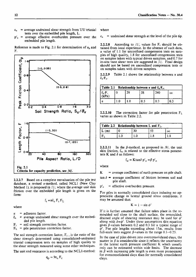
2.2.2.6 A further modification of the equations in 2.2.2.5 is recommended in /4/ by considering the pile length effect in addition to the cu/p'0 ratio. The average unit skin friction along the pil e shaft, fs, is then obtained from the equation:
fs = a p F c u
where
ap = peak friction coefficient, being a function of the ratio Cu/p'o-
F = length factor, being a function of the ratio L/D (D = pile diameter).
2.2.2.2 The unit end resistance, qp, of piles in mainly cohesive soils may as an average be taken equal to 9 times the undrained shear strength of the soil at the level of the pile tip, provided that the installation process has not re-duced the shear strength. The end resistance may, how-ever, be limited by the capacity of an internal soil plug in the pile. Where pile shoes are employed as a means of reducing soil plug friction during driving, an equivalent reduction of internal skin friction should be adopted in the assessment of unit end resistance. Experience indicates that size effects may be of importance also in cohesive
= average unit skin friction along pile shaft in layer i.
= shaft area of pile in layer i. = unit end resistance. = gross end area of pile.
where
12 Classification Notes — No. 30.4
cu = average undrained shear strength from UU triaxial tests over the embedded pile length, L.
p'0 = average effective overburden pressure over the embedded pile length.
Reference is made to Fig. 2.1 for determination of ap and F.
Fig. 2.1 Criteria for capacity prediction, see /4/.
2.2.2.7 Based on a complete reevaluation of the pile test database, a revised a-method, called NCL1 (New Clay Method 1), is proposed in / l / , where the average unit skin friction over the embedded pile length is given on the form:
where
a = adhesion factor. cu = average undrained shear strength over the embed-
ded pile length. FC = soil strength correction factor. F l = pile penetration correction factor.
The soil strength correction factor, FC , is the ratio of the shear strength determined using consolidated-undrained triaxial compression tests on samples of high quality to the shear strength measured using some other techniques. The unit end resistance is according to the NCL1-method:
qP = 9C U F C
where
cu = undrained shear strength at the level of the pile tip.
2.2.2.8 According to /l/ , values for Fc should be ob-tained from local experience. In the absence of such data, a value of 1.1 for unconfined compression tests on sam-ples of high quality, 1.8 for unconfined compression tests on samples taken with typical driven samplers, and 0.7 for in-situ vane shear tests are suggested in /I /. Final design should not be based on unconfined compression tests or on samples taken with driven samplers.
2.2.2.9 Table 2.1 shows the relationship between a and cu-Fc.
Table 2.1 Relationship between a and cuFc. Cu'Fc (kPa)
0 29 58 240 oo
a 1.0 1 . 0 0.5 0.3 0.3
2.2.2.10 The correction factor for pile penetration FL varies as shown in Table 2.2.
Table 2.2 Relationship between L and Fi.. L(m) 0 30 53 oo FL 1.0 1.0 1.8 1.8
2.2.2.11 In the j?-method, as proposed in /9/, the unit skin friction, fsi, is related to the effective stress parame-ters K and 5 as follows:
where
K = average coefficient of earth pressure on pile shaft. tan S = average coefficient of friction between soil and
pile shaft. p'0 = effective overburden pressure.
For piles in normally consolidated clays inducing no ap-preciable change in lateral ground stress conditions, it may be assumed that:
K = 1 — sin <j>'
If it is further assumed that failure takes place in the re-moulded soil close to the shaft surface, the remoulded, drained angle of shearing resistance may be used for q>' along with <5=</>'. Under these assumptions this equation gives jS-values between 0.2 and 0.3 for a typicai range of <£'. For pile lengths exceeding about 15m, results from full-scale tests suggest /^-values in the range 0.1—0.25. In the case of piles driven into overconsolidated clays, the scatter in is considerable since it reflects the uncertainty in the lateral earth pressure coefficient K which usually only can be estimated within wide limits. The decrease in /? with increasing pile length is even more pronounced for overconsolidated clays than for normally consolidated clays.
13 Classification Notes — No. 30.4
2.2.2.12 Other methods where the unit skin friction is considered a function of the effective overburden pressure is proposed in /12,13/.
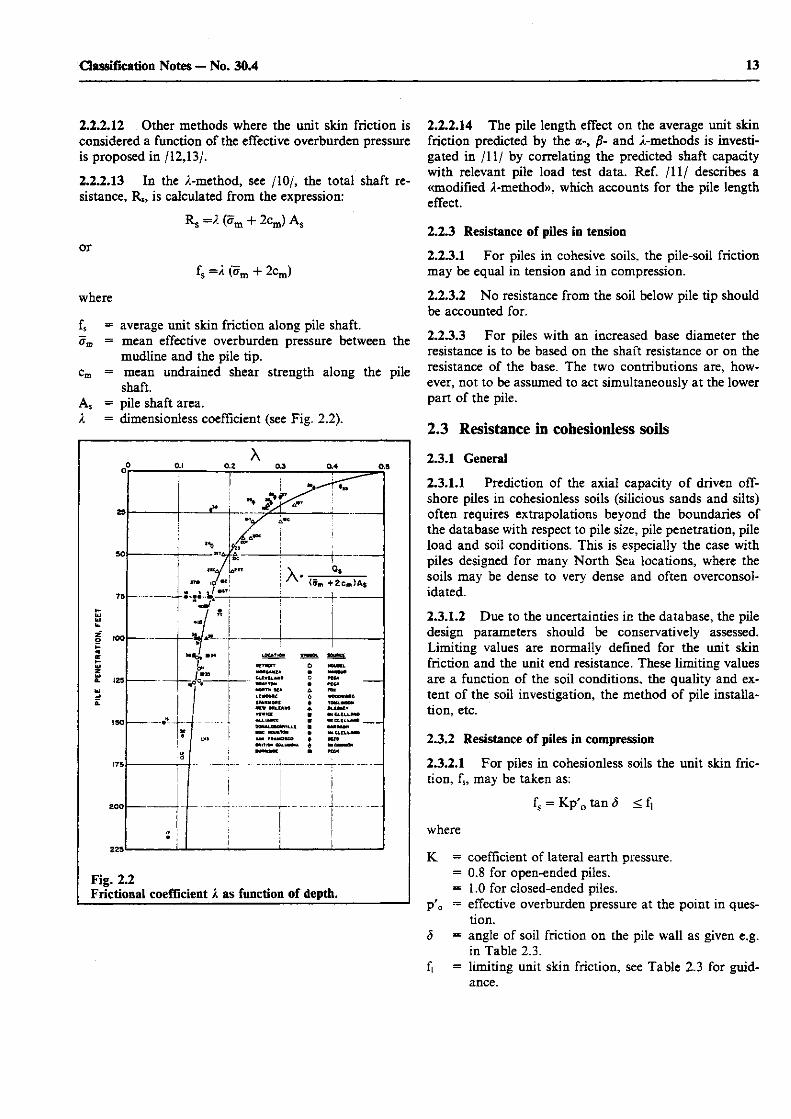
2.2.2.13 In the A-method, see /10/, the total shaft re-sistance, Rs, is calculated from the expression:
Rs=^(^m + 2cm)A s
or
f s + 2cm)
where
fs = average unit skin friction along pile shaft. am = mean effective overburden pressure between the
mudline and the pile tip. cm = mean undrained shear strength along the pile
shaft. As = pile shaft area. A = dimensionless coefficient (see Fig. 2.2).
2.2.2.14 The pile length effect on the average unit skin friction predicted by the a-, /?- and A-methods is investi-gated in / l l / by correlating the predicted shaft capacity with relevant pile load test data. Ref. / I I / describes a «modified A-method», which accounts for the pile length effect.
2.2.3 Resistance of piles in tension
2.2.3.1 For piles in cohesive soils, the pile-soil friction may be equal in tension and in compression.
2.2.3.2 No resistance from the soil below pile tip should be accounted for.
2.2.3.3 For piles with an increased base diameter the resistance is to be based on the shaft resistance or on the resistance of the base. The two contributions are, how-ever, not to be assumed to act simultaneously at the lower part of the pile.
2.3 Resistance in cohesionless soils
Fig. 2.2 Frictional coefficient A as function of depth.
2.3.1 General
2.3.1.1 Prediction of the axial capacity of driven off-shore piles in cohesionless soils (silicious sands and silts) often requires extrapolations beyond the boundaries of the database with respect to pile size, pile penetration, pile load and soil conditions. This is especially the case with piles designed for many North Sea locations, where the soils may be dense to very dense and often overconsol-idated.
2.3.1.2 Due to the uncertainties in the database, the pile design parameters should be conservatively assessed. Limiting values are normally defined for the unit skin friction and the unit end resistance. These limiting values are a function of the soil conditions, the quality and ex-tent of the soil investigation, the method of pile installa-tion, etc.
2.3.2 Resistance of piles in compression
2.3.2.1 For piles in cohesionless soils the unit skin fric-tion, fs, may be taken as:
fs = Kp'0 tan S < fj
where
K = coefficient of lateral earth pressure. = 0.8 for open-ended piles. = 1.0 for closed-ended piles.
p'0 = effective overburden pressure at the point in ques-tion.
<5 = angle of soil friction on the pile wall as given e.g. in Table 2.3.
fi = limiting unit skin friction, see Table 2.3 for guid-ance.
14 Classification Notes — No. 30.4
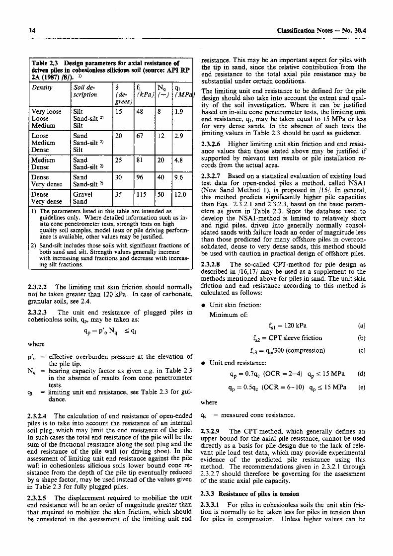
Table 2.3 D< driven piles in 2A (1987) /8/;
>sign parameters for axial resistance of cohesionless silicious soil (source: API RP
Density Soil de-scription
5 (de-grees)
fi (kPa)
Nq
( - ) qi (MPa
Very loose Loose Medium
Silt Sand-silt 2> Silt
15 48 8 1.9
Loose Medium Dense
Sand Sand-silt 2> Silt
20 67 12 2.9
Medium Dense
Sand Sand-silt 2>
25 81 20 4.8
Dense Very dense
Sand Sand-silt 2>
30 96 40 9.6
Dense Very dense
Gravel Sand
35 115 50 12.0
1) The parameters listed in this table are intended as guidelines only. Where detailed information such as in-situ cone penetrometer tests, strength tests on high quality soil samples, model tests or pile driving perform-ance is available, other values may be justified.
2) Sand-silt includes those soils with significant fractions of both sand and silt. Strength values generally increase with increasing sand fractions and decrease with increas-ing silt fractions.
2.3.2.2 The limiting unit skin friction should normally not be taken greater than 120 kPa. In case of carbonate, granular soils, see 2.4.
2.3.2.3 The unit end resistance of plugged piles in cohesionless soils, qp, may be taken as:
<lp = P 'oNq
where
p'o = effective overburden pressure at the elevation of the pile tip.
Nq = bearing capacity factor as given e.g. in Table 2.3 in the absence of results from cone penetrometer tests.
qi = limiting unit end resistance, see Table 2.3 for gui-dance.
2.3.2.4 The calculation of end resistance of open-ended piles is to take into account the resistance of an internal soil plug, which may limit the end resistance of the pile. In such cases the total end resistance of the pile will be the sum of the frictional resistance along the soil plug and the end resistance of the pile wall (or driving shoe). In the assessment of limiting unit end resistance against the pile wall in cohesionless silicious soils lower bound cone re-sistance from the depth of the pile tip eventually reduced by a shape factor, may be used instead of the values given in Table 2.3 for fully plugged piles.
2.3.2.5 The displacement required to mobilize the unit end resistance will be an order of magnitude greater than that required to mobilize the skin friction, which should be considered in the assessment of the limiting unit end
resistance. This may be an important aspect for piles with the tip in sand, since the relative contribution from the end resistance to the total axial pile resistance may be substantial under certain conditions. The limiting unit end resistance to be defined for the pile design should also take into account the extent and qual-ity of the soil investigation. Where it can be justified based on in-situ cone penetrometer tests, the limiting unit end resistance, qi, may be taken equal to 15 MPa or less for very dense sands. In the absence of such tests the limiting values in Table 2.3 should be used as guidance.
2.3.2.6 Higher limiting unit skin friction and end resist-ance values than those stated above may be justified if supported by relevant test results or pile installation re-cords from the actual area. 2.3.2.7 Based on a statistical evaluation of existing load test data for open-ended piles a method, called NSA1 (New Sand Method 1), is proposed in /15/. In general, this method predicts significantly higher pile capacities than Eqs. 2.3.2.1 and 2.3.2.3, based on the basic param-eters as given in Table 2.3. Since the database used to develop the NSA1-method is limited to relatively short and rigid piles, driven into generally normally consol-idated sands with failure loads an order of magnitude less than those predicted for many offshore piles in overcon-solidated, dense to very dense sands, this method should be used with caution in practical design of offshore piles.
2.3.2.8 The so-called CPT-method for pile design as described in /16,17/ may be used as a supplement to the methods mentioned above for piles in sand. The unit skin friction and end resistance according to this method is calculated as follows:
• Unit skin friction: Minimum of:
f s l = 120 kPa (a)
fs2 = CPT sleeve friction (b)
fs3 = qc/300 (compression) (c)
• Unit end resistance: qp = 0.7qc (OCR = 2-4) qp < 15 MPa (d)
qp = 0.5qc (OCR = 6-10) qp < 15 MPa (e)
where
qc = measured cone resistance.
2.3.2.9 The CPT-method, which generally defines an upper bound for the axial pile resistance, cannot be used directly as a basis for pile design due to the lack of rele-vant pile load test data, which may provide experimental evidence of the predicted pile resistance using this method. The recommendations given in 2.3.2.1 through 2.3.2.7 should therefore be governing for the assessment of the static axial pile capacity.
2.3.3 Resistance of piles in tension 2.3.3.1 For piles in cohesionless soils the unit skin fric-tion is normally to be taken less for piles in tension than for piles in compression. Unless higher values can be
15 Classification Notes — No. 30.4
shown to be justified, the coefficient of lateral earth pressure, K in 2.3.2.1, may be taken equal to 0.5 for piles in tension.
2.3.3.2 For piles with an increased base diameter, the resistance is to be based on the shaft resistance or on the resistance of the base. The two contributions are, how-ever, not to be assumed to act simultaneously at the lower part of the pile.
2.4 Resistance in calcareous soils
2.4.1 Driven piles
2.4.1.1 The axial capacity of driven piles in calcareous soils is calculated according to the same principles as adopted for piles in sands, except that the limiting unit skin friction and end resistance values are typically smal-ler. For guidance reference is made to /18/.
2.4.1.2 Factors of importance for assessment of limiting unit end and skin friction values are among others, the degree of cementation, grain crushability, relative density, compressive strength and carbonate content.
2.4.2 Drilled and grouted piles
2.4.2.1 Skin friction of drilled and grouted piles in cal-careous sands is usually higher than the friction mobilized by driven piles in the same formations. For guidance ref-erence is made to /18/.
2.4.2.2 Pile shaft resistance is limited by the shear strength of the pile/grout interface, the soil/grout inter-face or the soil itself
2.4.2.3 For cemented calcareous soil the ultimate shaft shear is often related to the unconfined compressive strength of the cemented soil.
2.4.2.4 Relationship between ultimate shaft shear and rock unconfined compressive strength to be used in ca-pacity calculations should be developed based on general experience from the location or pile load tests.
2.4.2.5 The contribution of the pile tip to the total pile capacity is dependent on a clean bottom hole.
2.5 Group effects
2.5.1 General
2.5.1.1 The group resistance of piles depends on factors such as pile spacing, type and strength of soils, sequence of soil layers, pile installation method, etc. The know-ledge of the behaviour of full-scale pile groups relative to the behaviour of individual piles in the same group is limited and conservative assumptions are therefore re-commended for the calculation of pile group resistance.
2.5.1.2 In estimating pile group resistance from a cal-culated single pile resistance, special considerations are required in each case in order to account for:
• Method of pile installation • Weak deposit underlying a bearing layer of limited
thickness • Negative skin friction along pile shaft.
2.5.1.3 In addition to the possible limitation of the group resistance, closely spaced piles will also influence the displacements of the individual piles which is of im-portance to consider for the interaction between the structure and the pile foundation. This can in principle be done by calculating the displacement of the soil sur-rounding one pile due to the loading from the other piles in the pile group. These displacements may be calculated based on elastic halfspace solutions for constant or steadily increasing shear modulus, ref. e.g. /24/. The un-certainties related to the selection of appropriate equiv-alent soil moduli should be considered, and the choice should be related to the general stress level in the soil volume within and outside the pile group.
2.5.2 Pile groups
2.5.2.1 For a given geometry and number of piles in a group, a transition zone of pile spacing exists within which the failure mechanism gradually changes from «pier» failure at small spacings to individual pile failure at larger spacings.
2.5.2.2 In case of a «pier» failure, the axial resistance of the pile group consists of skin friction along the outer perimeter of the group plus end bearing of the «pier».
2.5.2.3 «Solid» piers enclosing all soil within a pile group envelope (minimum pier circumference) as well as «hollow» piers (minimum pier area) should be considered when relevant. Limitations in tip resistance for the pier due to limitations in allowable displacements should be considered.
2.5.2.4 In the above calculations the unit skin friction fsi can be taken equal to the undrained shear strength cu in clay and tan<£ times in-situ horizontal effective pressure in sand where <f> is the angle of shearing resistance.
2.5.2.5 Full utilization of the end bearing capacity as calculated in 6.2.2 requires large vertical deformations. Thus, the allowable deformations govern the end resist-ance contribution to the total group resistance.
2.5.2.6 The undrained shear strength cu and the angle of shearing resistance <t> to be applied in the above calcu-lations should be carefully chosen. Remoulding of the clay and densification of the sand during pile installation affect these quantities.
2.6 Effects of installation procedure 2.6.1 General
2.6.1.1 Due consideration is to be given to the method of installation when calculating the axial pile capacity. The methods presented herein apply mainly to open-ended driven piles.
2.7 Effects of cyclic loading
2.7.1 General
2.7.1.1 The effects of cyclic loading on the axial pile resistance and displacement should be considered in the design. The main objective is to determine the shear strength degradation along the pile shaft for different loading intensities.
16 Classification Notes — No. 30.4
2.7.1.2 The effects of cyclic loading are most significant for piles in cohesive soils, in cemented calcareous soils and in finegrained cohesionless soils (silt), whereas these effects are much less in medium- to coarsegrained cohe-sionless soils. The remoulding of the soil due to pile in-stallation and the subsequent time dependent reconsolidation of the soil are important factors in the evaluation of the effects of cyclic loading in finegrained soils.
2.7.2 Evaluation of the cyclic effects
2.7.2.1 The most important factors to be considered in modelling of cyclic axial loading of piles are:
• Type of cyclic loading (one-way vs. two-way, load-controlled vs. displacement-controlled) and number of cycles (at various stress levels)
• Soil properties and variation of soil strength and stiff-ness with depth
• Pile flexibility and pile length • Static stress distribution along the pile before cyclic
loading • Compatibility in terms of both cyclic and average dis-
placements and stresses.
See also 2.2.1.4—2.2.1.6.
2.7.2.2 For cohesive soils comprehensive research has been performed with respect to the analysis of piles sub-jected to combined static and cyclic loadings. Reference is made to /6,19/ for guidance on how to assess the effects of cyclic loading. Due to the uncertainties involved in modelling and analyzing the effects of cyclic loading the design methods proposed in the literature are normally based on a theoretical framework, which has been cali-brated against the results from small to large scale pile tests in various types of soil.
2.7.2.3 For calcareous soils the effects of cyclic loading on the capacity of both driven and drilled and grouted piles may be significant and should be evaluated from case to case for local conditions. For guidance, reference is made to /18/.
3. Lateral Pile Resistance 3.1 Introduction
3.1.1 General
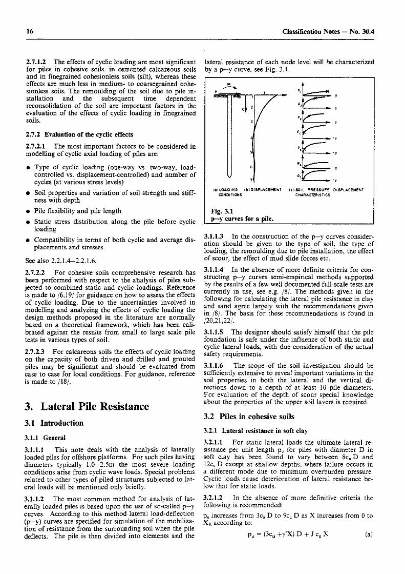
3.1.1.1 This note deals with the analysis of laterally loaded piles for offshore platforms. For such piles having diameters typically 1.0—2.5m the most severe loading conditions arise from cyclic wave loads. Special problems related to other types of piled structures subjected to lat-eral loads will be mentioned only briefly.
3.1.1.2 The most common method for analysis of lat-erally loaded piles is based upon the use of so-called p—y curves. According to this method lateral load-deflection (p-y) curves are specified for simulation of the mobiliza-tion of resistance from the surrounding soil when the pile deflects. The pile is then divided into elements and the
lateral resistance of each node level will be characterized by a p—y curve, see Fig. 3.1.
3.1.1.3 In the construction of the p—y curves consider-ation should be given to the type of soil, the type of loading, the remoulding due to pile installation, the effect of scour, the effect of mud slide forces etc.
3.1.1.4 In the absence of more definite criteria for con-structing p—y curves semi-empirical methods supported by the results of a few well documented full-scale tests are currently in use, see e.g. /8/. The methods given in the following for calculating the lateral pile resistance in clay and sand agree largely with the recommendations given in /8/. The basis for these recommendations is found in /20,21,22/.
3.1.1.5 The designer should satisfy himself that the pile foundation is safe under the influence of both static and cyclic lateral loads, with due consideration of the actual safety requirements.
3.1.1.6 The scope of the soil investigation should be sufficiently extensive to reveal important variations in the soil properties in both the lateral and the vertical di-rections down tc a depth of at least 10 pile diameters. For evaluation of the depth of scour special knowledge about the properties of the upper soil layers is required.
3.2 Piles in cohesive soils 3.2.1 Lateral resistance in soft clay
3.2.1.1 For static lateral loads the ultimate lateral re-sistance per unit length pu for piles with diameter D in soft clay has been found to vary between 8cu D and 12cu D except at shallow depths, where failure occurs in a different mode due to minimum overburden pressure. Cyclic loads cause deterioration of lateral resistance be-low that for static loads.
3.2.1.2 In the absence of more definitive criteria the following is recommended: pu increases from 3ca D to 9cu D as X increases from 0 to XR according to:
Pu = (3cu + / X ) D + J cu X (a)
17 Classification Notes — No. 30.4
and
pu = 9cu D for X > XR (b)
where
pu = ultimate resistance per unit length (kN/m). cu = undrained shear strength for undisturbed clay soil
samples (kPa). D = pile diameter (m). y' = effective unit weight of soil (kN/m3). J = dimensionless empirical coefficient with values in
the range 0.25—0.50. The upper limit holds for soft normally consolidated cohesive soils.
X = depth below soil surface (m). XR = depth below soil surface to bottom of reduced re-
sistance zone in m. For a condition of constant strength with depth Eqs. (a) and (b) are solved si-multaneously to give:
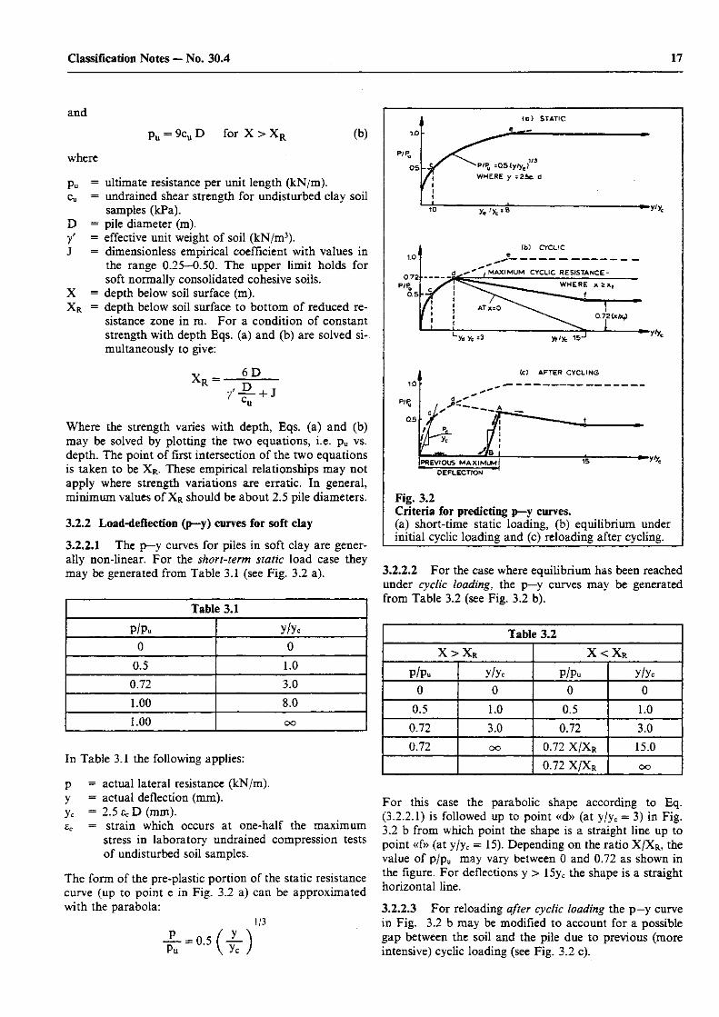
Fig. 3.2 Criteria for predicting p—y curves. (a) short-time static loading, (b) equilibrium under initial cyclic loading and (c) reloading after cycling.
6 D
Where the strength varies with depth, Eqs. (a) and (b) may be solved by plotting the two equations, i.e. pu vs. depth. The point of first intersection of the two equations is taken to be XR. These empirical relationships may not apply where strength variations are erratic. In general, minimum values of XR should be about 2.5 pile diameters.
3.2.2 Load-deflection (p—y) curves for soft clay
3.2.2.1 The p—y curves for piles in soft clay are gener-ally non-linear. For the short-term static load case they may be generated from Table 3.1 (see Fig. 3.2 a).
Table 3.1
P/Pu y/yc 0 0
0.5 1.0 0.72 3.0 1.00 8.0 1.00 oo
In Table 3.1 the following applies:
p = actual lateral resistance (kN/m). y = actual deflection (mm). yc = 2.5 ec D (mm). £c = strain which occurs at one-half the maximum
stress in laboratory undrained compression tests of undisturbed soil samples.
The form of the pre-plastic portion of the static resistance curve (up to point e in Fig. 3.2 a) can be approximated with the parabola:
1/3
= 0.5 ( — ^ Pu \ yc /
3.2.2.2 For the case where equilibrium has been reached under cyclic loading, the p—y curves may be generated from Table 3.2 (see Fig. 3.2 b).
Table 3.2 x > x R x < x R
P/Pu y/yc P/Pu y/yc 0 0 0 0
0.5 1.0 0.5 1.0 0.72 3.0 0.72 3.0 0.72 oo 0.72 X/XR 15.0
0.72 X/XR oo
For this case the parabolic shape according to Eq. (3.2.2.1) is followed up to point «d» (at y/yc = 3) in Fig. 3.2 b from which point the shape is a straight line up to point «f» (at y/yc = 15). Depending on the ratio X/XR, the value of p/pu may vary between 0 and 0.72 as shown in the figure. For deflections y > 15yc the shape is a straight horizontal line.
3.2.2.3 For reloading after cyclic loading the p—y curve in Fig. 3.2 b may be modified to account for a possible gap between the soil and the pile due to previous (more intensive) cyclic loading (see Fig. 3.2 c).
18 Classification Notes — No. 30.4
3.2.3 Lateral resistance in stiff clay
3.2.3.1 For static lateral loads the ultimate unit lateral resistance pu of stiff clay (cu > 100 kPa) would vary be-tween 8cu and 12cu as for soft clay.
3.2.3.2 Due to rapid deterioration under cyclic loadings the ultimate resistance will be reduced to something con-siderably less and should be so considered in cyclic design.
3.2.4 Load-deflection (p—y) curves for stiff clay
3.2.4.1 While stiff clays also have non-linear stress-strain relationships, they are generally more brittle than soft clays. In developing stress-strain curves and subse-quent p—y curves for cyclic loads, good judgement should reflect the rapid deterioration of lateral resistance at large deflections for stiff clays.
3.3 Piles in cohesionless soils
3.3.1 Lateral resistance in sand
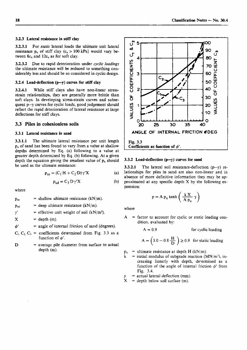
3.3.1.1 The ultimate lateral resistance per unit length pu of sand has been found to vary from a value at shallow depths determined by Eq. (a) following to a value at greater depth determined by Eq. (b) following. At a given depth the equation giving the smallest value of pu should be used as the ultimate resistance:
pus = (C,H + C 2 D ) 7 ' X
pud = C3 Dy'X
(a)
(b)
where
Pus = shallow ultimate resistance (kN/m).
Pud = deep ultimate resistance (kN/m).
/ = effective unit weight of soil (kN/m3).
X = depth (m).
4>' = angle of internal friction of sand (degrees).
Ci, C2, C3 = coefficients determined from Fig. 3.3 as a function of <p
D = average pile diameter from surface to actual depth (m).
p = A pu tanh
where
A =
P u
k
y x
factor to account for cyclic or static loading con-dition, evaluated by:
A = 0.9 for cyclic loading
A = ^3.0 - 0.8 - j j ^ > 0.9 for static loading
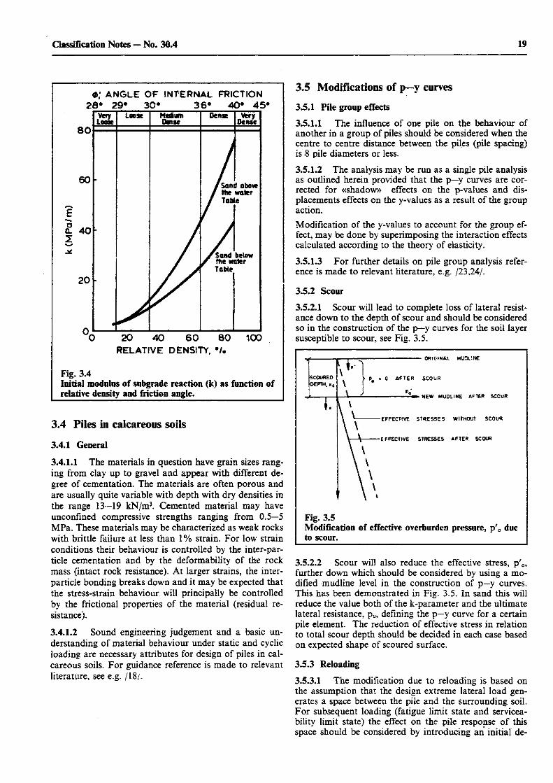
ultimate resistance at depth H (kN/'m). initial modulus of subgrade reaction (MN/m3), in-creasing linearly with depth, determined as a function of the angle of internal friction 4>' from Fig. 3.4. actual lateral deflection (mm), depth below soil surface (m).
3.3.2 Load-deflection (p—y) curves for sand
3.3.2.1 The lateral soil resistance-deflection (p—y) re-lationships for piles in sand are also non-linear and in absence of more definitive information they may be ap-proximated at any specific depth X by the following ex-pression:
19 Classification Notes — No. 30.4
3,5 Modifications of p—y curves 3.5.1 Pile group effects
3.5.1.1 The influence of one pile on the behaviour of another in a group of piles should be considered when the centre to centre distance between the piles (pile spacing) is 8 pile diameters or less.
3.5.1.2 The analysis may be run as a single pile analysis as outlined herein provided that the p—y curves are cor-rected for «shadow» effects on the p-values and dis-placements effects on the y-values as a result of the group action. Modification of the y-values to account for the group ef-fect, may be done by superimposing the interaction effects calculated according to the theory of elasticity.
3.5.1.3 For further details on pile group analysis refer-ence is made to relevant literature, e.g. /23,24/.
3.5.2 Scour
3.5.2.1 Scour will lead to complete loss of lateral resist-ance down to the depth of scour and should be considered so in the construction of the p—y curves for the soil layer susceptible to scour, see Fig. 3.5.
3.4 Piles in calcareous soils
3.4.1 General
3.4.1.1 The materials in question have grain sizes rang-ing from clay up to gravel and appear with different de-gree of cementation. The materials are often porous and are usually quite variable with depth with dry densities in the range 13—19 kN/m3. Cemented material may have unconfined compressive strengths ranging from 0.5—5 MPa. These materials may be characterized as weak rocks with brittle failure at less than 1 % strain. For low strain conditions their behaviour is controlled by the inter-par-ticle cementation and by the deformability of the rock mass (intact rock resistance). At larger strains, the inter-particle bonding breaks down and it may be expected that the stress-strain behaviour will principally be controlled by the frictional properties of the material (residual re-sistance).
3.4.1.2 Sound engineering judgement and a basic un-derstanding of material behaviour under static and cyclic loading are necessary attributes for design of piles in cal-careous soils. For guidance reference is made to relevant literature, see e.g. /18/.
3.5.2.2 Scour will also reduce the effective stress, p'0, further down which should be considered by using a mo-dified mudline level in the construction of p—y curves. This has been demonstrated in Fig. 3.5. In sand this will reduce the value both of the k-parameter and the ultimate lateral resistance, pu, defining the p—y curve for a certain pile element. The reduction of effective stress in relation to total scour depth should be decided in each case based on expected shape of scoured surface.
3.5.3 Reloading
3.5.3.1 The modification due to reloading is based on the assumption that the design extreme lateral load gen-erates a space between the pile and the surrounding soil. For subsequent loading (fatigue limit state and servicea-bility limit state) the effect on the pile response of this space should be considered by introducing an initial de-
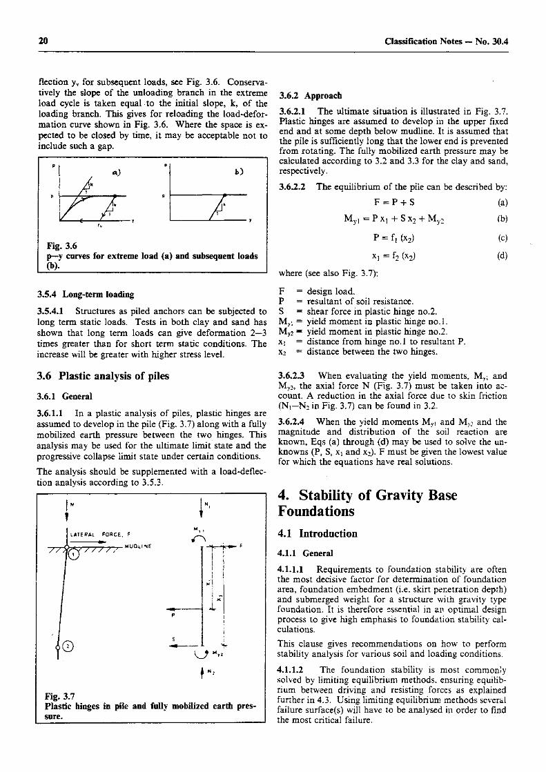
20 Classification Notes — No. 30.4
flection yv for subsequent loads, see Fig. 3.6. Conserva-tively the slope of the unloading branch in the extreme load cycle is taken equal to the initial slope, k, of the loading branch. This gives for reloading the load-defor-mation curve shown in Fig. 3.6. Where the space is ex-pected to be closed by time, it may be acceptable not to include such a gap.
Fig. 3.6 p—y curves for extreme load (a) and subsequent loads (b).
3.5.4 Long-term loading
3.5.4.1 Structures as piled anchors can be subjected to long term static loads. Tests in both clay and sand has shown that long term loads can give deformation 2—3 times greater than for short term static conditions. The increase will be greater with higher stress level.
3.6.2 Approach
3.6.2.1 The ultimate situation is illustrated in Fig. 3.7. Plastic hinges are assumed to develop in the upper fixed end and at some depth below mudline. It is assumed that the pile is sufficiently long that the lower end is prevented from rotating. The fully mobilized earth pressure may be calculated according to 3.2 and 3.3 for the clay and sand, respectively.
3.6.2.2 The equilibrium of the pile can be described by:
F = P + S (a)
My l = P xj + S x2 + My2 (b)
P = fi (x2) (c)
x, = f2 (x2) (d)
where (see also Fig. 3.7):
F = design load. P = resultant of soil resistance. S = shear force in plastic hinge no.2. Myi = yield moment in plastic hinge no.l. My2 = yield moment in plastic hinge no.2. xi = distance from hinge no.l to resultant P. x2 = distance between the two hinges.
3.6 Plastic analysis of piles
3.6.1 General
3.6.1.1 In a plastic analysis of piles, plastic hinges are assumed to develop in the pile (Fig. 3.7) along with a fully mobilized earth pressure between the two hinges. This analysis may be used for the ultimate limit state and the progressive collapse limit state under certain conditions.
The analysis should be supplemented with a load-deflec-tion analysis according to 3.5.3.
J- i-
Fig. 3.7 Plastic hinges in pile and fully mobilized earth pres-sure.
3.6.2.3 When evaluating the yield moments, Myi and My2, the axial force N (Fig. 3.7) must be taken into ac-count. A reduction in the axial force due to skin friction (Ni—N2 in Fig. 3.7) can be found in 3.2.
3.6.2.4 When the yield moments Myi and My2 and the magnitude and distribution of the soil reaction are known, Eqs (a) through (d) may be used to solve the un-knowns (P, S, xi and x2). F must be given the lowest value for which the equations have real solutions.
4. Stability of Gravity Base Foundations 4.1 Introduction 4.1.1 General
4.1.1.1 Requirements to foundation stability are often the most decisive factor for determination of foundation area, foundation embedment (i.e. skirt penetration depth) and submerged weight for a structure with gravity type foundation. It is therefore essential in an optimal design process to give high emphasis to foundation stability cal-culations. This clause gives recommendations on how to perform stability analysis for various soil and loading conditions.
4.1.1.2 The foundation stability is most commonly solved by limiting equilibrium methods, ensuring equilib-rium between driving and resisting forces as explained further in 4.3. Using limiting equilibrium methods several failure surface(s) will have to be analysed in order to find the most critical failure.
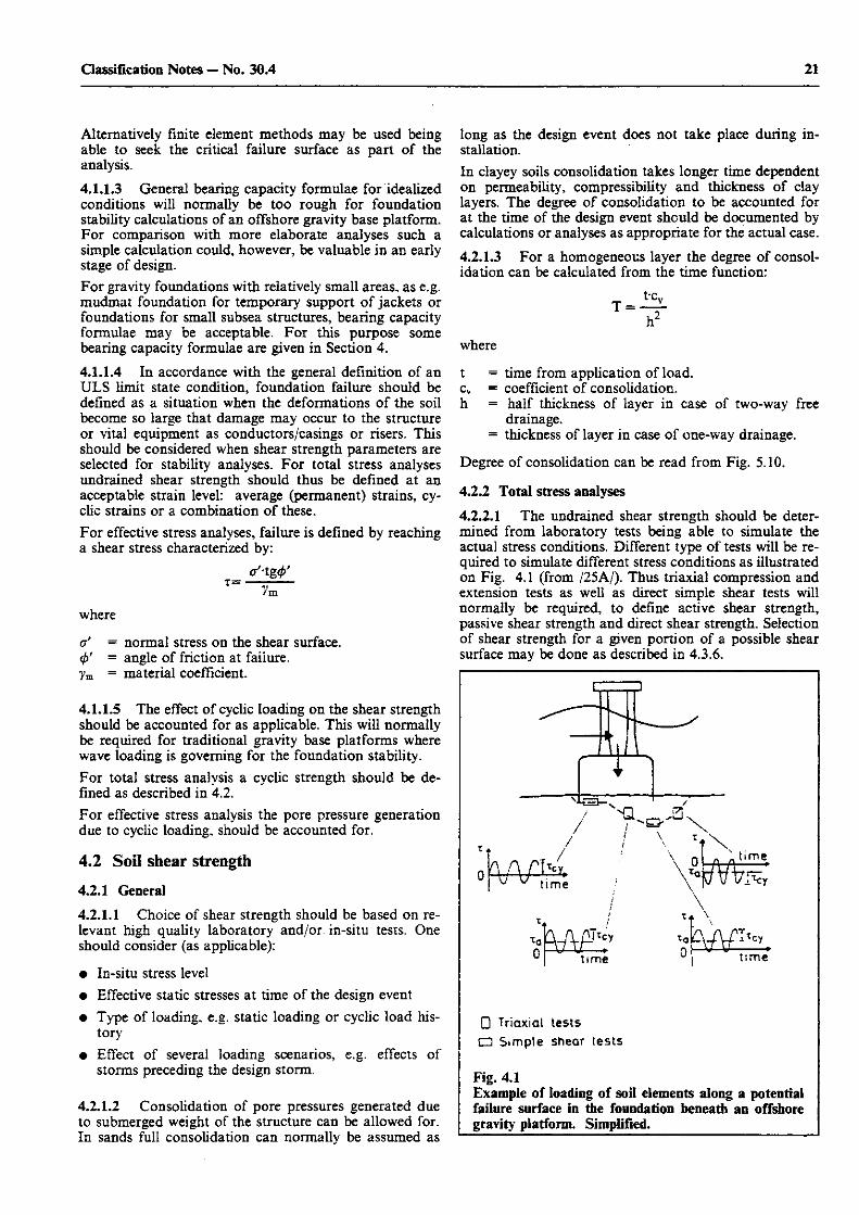
21 Classification Notes — No. 30.4
Alternatively finite element methods may be used being able to seek the critical failure surface as part of the analysis. 4.1.1.3 General bearing capacity formulae for idealized conditions will normally be too rough for foundation stability calculations of an offshore gravity base platform. For comparison with more elaborate analyses such a simple calculation could, however, be valuable in an early stage of design. For gravity foundations with relatively small areas, as e.g. mudmat foundation for temporary support of jackets or foundations for small subsea structures, bearing capacity formulae may be acceptable. For this purpose some bearing capacity formulae are given in Section 4.
4.1.1.4 In accordance with the general definition of an ULS limit state condition, foundation failure should be defined as a situation when the deformations of the soil become so large that damage may occur to the structure or vital equipment as conductors/casings or risers. This should be considered when shear strength parameters are selected for stability analyses. For total stress analyses undrained shear strength should thus be defined at an acceptable strain level: average (permanent) strains, cy-clic strains or a combination of these. For effective stress analyses, failure is defined by reaching a shear stress characterized by:
T = • c'tgP
7m where
long as the design event does not take place during in-stallation. In clayey soils consolidation takes longer time dependent on permeability, compressibility and thickness of clay layers. The degree of consolidation to be accounted for at the time of the design event should be documented by calculations or analyses as appropriate for the actual case.
4.2.1.3 For a homogeneous layer the degree of consol-idation can be calculated from the time function:
T = t-cv
where
& = normal stress on the shear surface. = angle of friction at failure.
ym = material coefficient.
4.1.1.5 The effect of cyclic loading on the shear strength should be accounted for as applicable. This will normally be required for traditional gravity base platforms where wave loading is governing for the foundation stability. For total stress analysis a cyclic strength should be de-fined as described in 4.2. For effective stress analysis the pore pressure generation due to cyclic loading, should be accounted for.
4.2 Soil shear strength 4.2.1 General 4.2.1.1 Choice of shear strength should be based on re-levant high quality laboratory and/or in-situ tests. One should consider (as applicable):
• In-situ stress level • Effective static stresses at time of the design event • Type of loading, e.g. static loading or cyclic load his-
tory • Effect of several loading scenarios, e.g. effects of
storms preceding the design storm.
4.2.1.2 Consolidation of pore pressures generated due to submerged weight of the structure can be allowed for. In sands full consolidation can normally be assumed as
t = time from application of load. cv = coefficient of consolidation, h = half thickness of layer in case of two-way free
drainage.
= thickness of layer in case of one-way drainage.
Degree of consolidation can be read from Fig. 5.10.
4.2.2 Total stress analyses 4.2.2.1 The undrained shear strength should be deter-mined from laboratory tests being able to simulate the actual stress conditions. Different type of tests will be re-quired to simulate different stress conditions as illustrated on Fig. 4.1 (from /25A/). Thus triaxial compression and extension tests as well as direct simple shear tests will normally be required, to define active shear strength, passive shear strength and direct shear strength. Selection of shear strength for a given portion of a possible shear surface may be done as described in 4.3.6.
t:me
• Triaxial tests
• Simple shear tests
Fig. 4.1 Example of loading of soil elements along a potential failure surface in the foundation beneath an offshore gravity platform. Simplified.
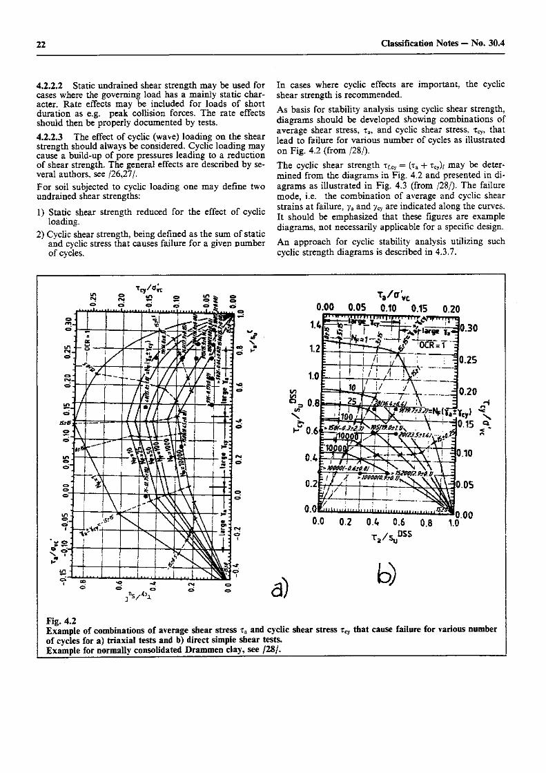
22 Classification Notes — No. 30.4
4.2.2.2 Static undrained shear strength may be used for cases where the governing load has a mainly static char-acter. Rate effects may be included for loads of short duration as e.g. peak collision forces. The rate effects should then be properly documented by tests. 4.2.2.3 The effect of cyclic (wave) loading on the shear strength should always be considered. Cyclic loading may cause a build-up of pore pressures leading to a reduction of shear strength. The general effects are described by se-veral authors, see /26,27/. For soil subjected to cyclic loading one may define two undrained shear strengths:
1) Static shear strength reduced for the effect of cyclic loading.
2) Cyclic shear strength, being defined as the sum of static and cyclic stress that causes failure for a given number of cycles.
In cases where cyclic effects are important, the cyclic shear strength is recommended. As basis for stability analysis using cyclic shear strength, diagrams should be developed showing combinations of average shear stress, ia, and cyclic shear stress, Tcy, that lead to failure for various number of cycles as illustrated on Fig. 4.2 (from /28/). The cyclic shear strength if,cy = (ra -I- Tcy)r may be deter-mined from the diagrams in Fig. 4.2 and presented in di-agrams as illustrated in Fig. 4.3 (from /28/). The failure mode, i.e. the combination of average and cyclic shear strains at failure, ya and ycy are indicated along the curves. It should be emphasized that these figures are example diagrams, not necessarily applicable for a specific design. An approach for cyclic stability analysis utilizing such cyclic strength diagrams is described in 4.3.7.
x
V f f ' v c 0.00 0.05 0.10 0.15 0 20
Mum ii Ulii in
0.0 0.2 0.4 0.6 o 8
T a / S * 5
a) b)
Fig. 4.2 Example of combinations of average shear stress ia and cyclic shear stress rcy that cause failure for various number of cycles for a) triaxial tests and b) direct simple shear tests. Example for normally consolidated Drammen clay, see /28/.
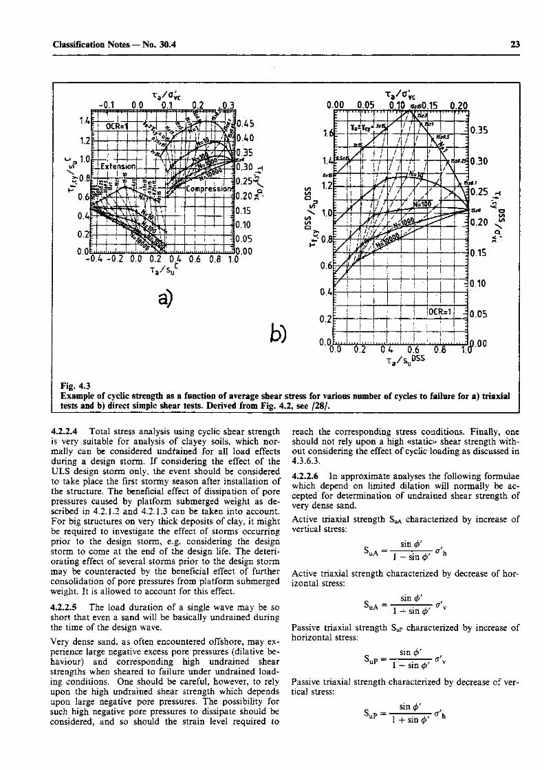
23 Classification Notes — No. 30.4
a)
b) .0 0.2 0.4 0.6 0.8 1.
x / s DSS
Fig. 4.3 Example of cyclic strength as a function of average shear stress for various number of cycles to failure for a) triaxial tests and b) direct simple shear tests. Derived from Fig. 4.2, see /28/.
4.2.2.4 Total stress analysis using cyclic shear strength is very suitable for analysis of clayey soils, which nor-mally can be considered undfained for all load effects during a design storm. If considering the effect of the ULS design storm only, the event should be considered to take place the first stormy season after installation of the structure. The beneficial effect of dissipation of pore pressures caused by platform submerged weight as de-scribed in 4.2.1.2 and 4.2.1.3 can be taken into account. For big structures on very thick deposits of clay, it might be required to investigate the effect of storms occurring prior to the design storm, e.g. considering the design storm to come at the end of the design life. The deteri-orating effect of several storms prior to the design storm may be counteracted by the beneficial effect of further consolidation of pore pressures from platform submerged weight. It is allowed to account for this effect.
4.2.2.5 The load duration of a single wave may be so short that even a sand will be basically undrained during the time of the design wave. Very dense sand, as often encountered offshore, may ex-perience large negative excess pore pressures (dilative be-haviour) and corresponding high undrained shear strengths when sheared to failure under undrained load-ing conditions. One should be careful, however, to rely upon the high undrained shear strength which depends upon large negative pore pressures. The possibility for such high negative pore pressures to dissipate should be considered, and so should the strain level required to
reach the corresponding stress conditions. Finally, one should not rely upon a high «static» shear strength with-out considering the effect of cyclic loading as discussed in 4.3.6.3.
4.2.2.6 In approximate analyses the following formulae which depend on limited dilation will normally be ac-cepted for determination of undrained shear strength of very dense sand. Active triaxial strength SUA characterized by increase of vertical stress:
SuA = sin <\>'
1 — sin <f> 7 ° h
Active triaxial strength characterized by decrease of hor-izontal stress:
_ sin 4>' ^uA - i , - i, ° v 1 4- sin <p
Passive triaxial strength Sup characterized by increase of horizontal stress:
SuP sin ()>'
1 — sin <(>'
Passive triaxial strength characterized by decrease of ver-tical stress:
SuP = " sin <j>'
1 + sin 4V
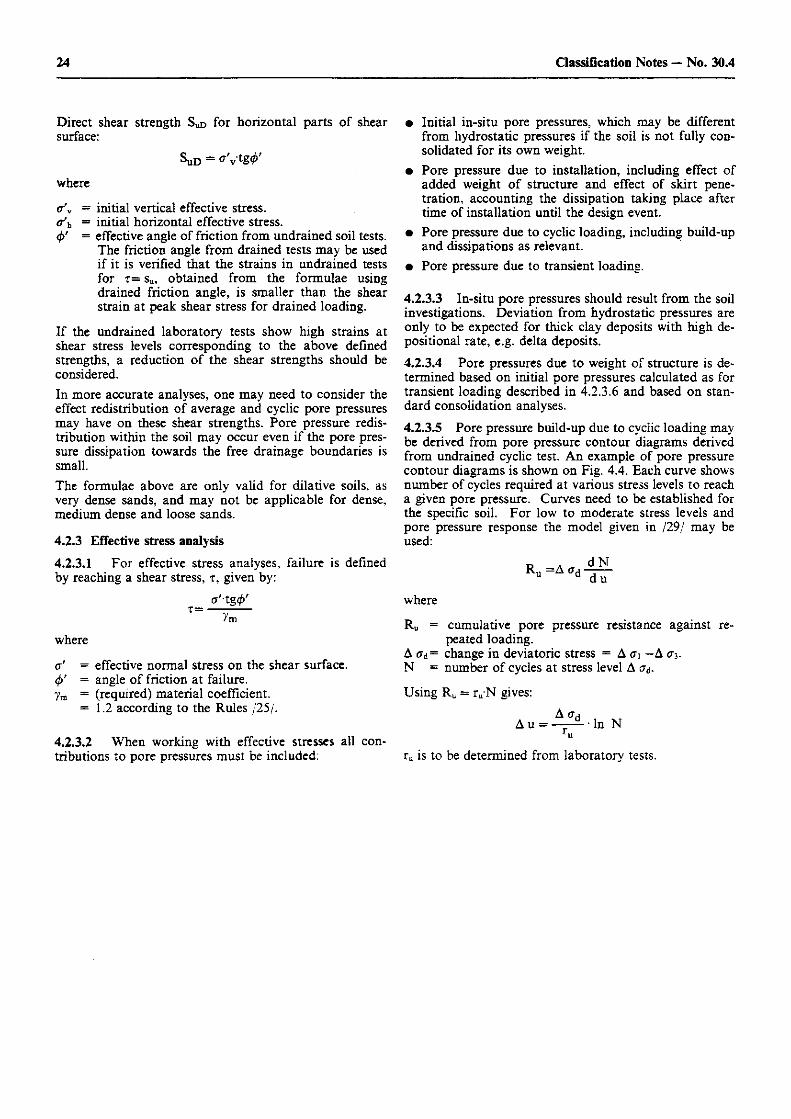
24 Classification Notes — No. 30.4
Direct shear strength SuD for horizontal parts of shear surface:
SUD = ff'vtg^' where
tr'v <r'h
4>'
initial vertical effective stress, initial horizontal effective stress, effective angle of friction from undrained soil tests. The friction angle from drained tests may be used if it is verified that the strains in undrained tests for T== su, obtained from the formulae using drained friction angle, is smaller than the shear strain at peak shear stress for drained loading.
If the undrained laboratory tests show high strains at shear stress levels corresponding to the above defined strengths, a reduction of the shear strengths should be considered. In more accurate analyses, one may need to consider the effect redistribution of average and cyclic pore pressures may have on these shear strengths. Pore pressure redis-tribution within the soil may occur even if the pore pres-sure dissipation towards the free drainage boundaries is small. The formulae above are only valid for dilative soils, as very dense sands, and may not be applicable for dense, medium dense and loose sands.
4.2.3 Effective stress analysis 4.2.3.1 For effective stress analyses, failure is defined by reaching a shear stress, t , given by:
a'-tg<t>' T = •
where
& = effective normal stress on the shear surface. (f>f = angle of friction at failure. 7m = (required) material coefficient.
= 1.2 according to the Rules /25/.
4.2.3.2 When working with effective stresses all con-tributions to pore pressures must be included:
• Initial in-situ pore pressures, which may be different from hydrostatic pressures if the soil is not fully con-solidated for its own weight.
• Pore pressure due to installation, including effect of added weight of structure and effect of skirt pene-tration, accounting the dissipation taking place after time of installation until the design event.
• Pore pressure due to cyclic loading, including build-up and dissipations as relevant.
• Pore pressure due to transient loading.
4.2.3.3 In-situ pore pressures should result from the soil investigations. Deviation from hydrostatic pressures are only to be expected for thick clay deposits with high de-positional rate, e.g. delta deposits. 4.2.3.4 Pore pressures due to weight of structure is de-termined based on initial pore pressures calculated as for transient loading described in 4.2.3.6 and based on stan-dard consolidation analyses.
4.2.3.5 Pore pressure build-up due to cyclic loading may be derived from pore pressure contour diagrams derived from undrained cyclic test. An example of pore pressure contour diagrams is shown on Fig. 4.4. Each curve shows number of cycles required at various stress levels to reach a given pore pressure. Curves need to be established for the specific soil. For low to moderate stress levels and pore pressure response the model given in /29/ may be used:
Ru =A crd d N d u
where
Ru = cumulative pore pressure resistance against re-peated loading.
A <7d= change in deviatoric stress = A G\ —A 03. N = number of cycles at stress level A (7d.
Using Ru = ru N gives: A Oa
A u = — - I n N ru ru is to be determined from laboratory tests.
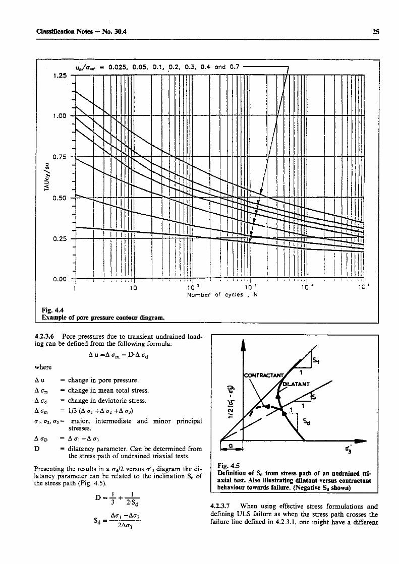
25 Classification Notes — No. 30.4
Fig. 4.4 Example of pore pressure contour diagram.
4.2.3.6 Pore pressures due to transient undrained load-ing can be defined from the following formula:
A u =A <rm — D A ad
where
A u = change in pore pressure. A am = change in mean total stress. A Od = change in deviatoric stress. A crm = 1/3 (A (71 +A cr2 +A <r3) <71,02,03= maJor> intermediate and minor principal
stresses. A <7D = A <J\ —A (73 D = dilatancy parameter. Can be determined from
the stress path of undrained triaxial tests.
Presenting the results in a <7d/2 versus <7'3 diagram the di-latancy parameter can be related to the inclination Sd of the stress path (Fig. 4.5).
D =
SH =
1 1 2-Sh
A(7 J — A<73
2Kc%
Fig. 4.5 Definition of Sd from stress path of an undrained tri-axial test. Also illustrating dilatant versus contractant behaviour towards failure. (Negative Sd shown)
4.2.3.7 When using effective stress formulations and defining ULS failure as when the stress path crosses the failure line defined in 4.2.3.1, one might have a different
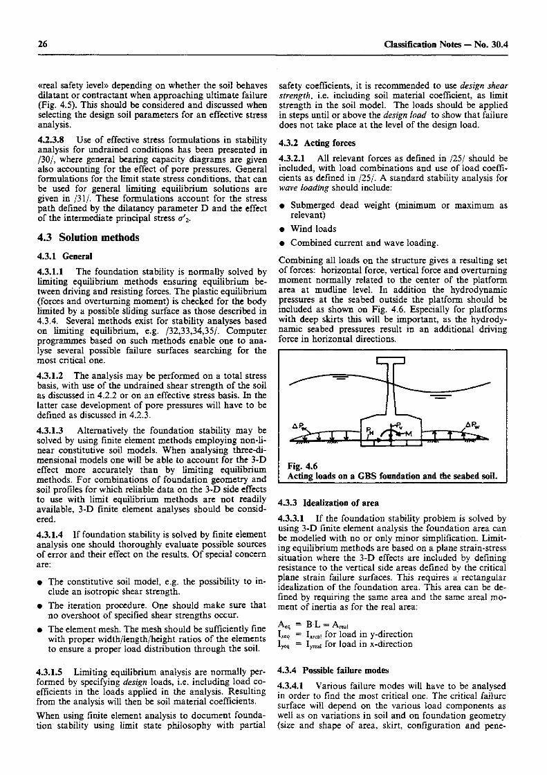
26 Classification Notes — No. 30.4
«real safety ievel» depending on whether the soil behaves dilatant or contractant when approaching ultimate failure (Fig. 4.5). This should be considered and discussed when selecting the design soil parameters for an effective stress analysis.
4.2.3.8 Use of effective stress formulations in stability analysis for undrained conditions has been presented in /30/, where general bearing capacity diagrams are given also accounting for the effect of pore pressures. General formulations for the limit state stress conditions, that can be used for general limiting equilibrium solutions are given in /31/. These formulations account for the stress path defined by the dilatancy parameter D and the effect of the intermediate principal stress <T'2.
4.3 Solution methods 4.3.1 General 4.3.1.1 The foundation stability is normally solved by limiting equilibrium methods ensuring equilibrium be-tween driving and resisting forces. The plastic equilibrium (forces and overturning moment) is checked for the body limited by a possible sliding surface as those described in 4.3.4. Several methods exist for stability analyses based on limiting equilibrium, e.g. /32,33,34,35/. Computer programmes based on such methods enable one to ana-lyse several possible failure surfaces searching for the most critical one.
4.3.1.2 The analysis may be performed on a total stress basis, with use of the undrained shear strength of the soil as discussed in 4.2.2 or on an effective stress basis. In the latter case development of pore pressures will have to be defined as discussed in 4.2.3.
4.3.1.3 Alternatively the foundation stability may be solved by using finite element methods employing non-li-near constitutive soil models. When analysing three-di-mensional models one will be able to account for the 3-D effect more accurately than by limiting equilibrium methods. For combinations of foundation geometry and soil profiles for which reliable data on the 3-D side effects to use with limit equilibrium methods are not readily available, 3-D finite element analyses should be consid-ered.
4.3.1.4 If foundation stability is solved by finite element analysis one should thoroughly evaluate possible sources of error and their effect on the results. Of special concern are:
• The constitutive soil model, e.g. the possibility to in-clude an isotropic shear strength.
• The iteration procedure. One should make sure that no overshoot of specified shear strengths occur.
• The element mesh. The mesh should be sufficiently fine with proper width/length/height ratios of the elements to ensure a proper load distribution through the soil.
4.3.1.5 Limiting equilibrium analysis are normally per-formed by specifying design loads, i.e. including load co-efficients in the loads applied in the analysis. Resulting from the analysis will then be soil material coefficients. When using finite element analysis to document founda-tion stability using limit state philosophy with partial
safety coefficients, it is recommended to use design shear strength, i.e. including soil material coefficient, as limit strength in the soil model. The loads should be applied in steps until or above the design load to show that failure does not take place at the level of the design load.
4.3.2 Acting forces 4.3.2.1 All relevant forces as defined in /25/ should be included, with load combinations and use of load coeffi-cients as defined in /25/. A standard stability analysis for wave loading should include:
• Submerged dead weight (minimum or maximum as relevant)
• Wind loads • Combined current and wave loading.
Combining all loads on the structure gives a resulting set of forces: horizontal force, vertical force and overturning moment normally related to the center of the platform area at mudline level. In addition the hydrodynamic pressures at the seabed outside the platform should be included as shown on Fig. 4.6. Especially for platforms with deep skirts this will be important, as the hydrody-namic seabed pressures result in an additional driving force in horizontal directions.
Acting loads on a GBS foundation and the seabed soil.
4.3.3 Idealization of area 4.3.3.1 If the foundation stability problem is solved by using 3-D finite element analysis the foundation area can be modelled with no or only minor simplification. Limit-ing equilibrium methods are based on a plane strain-stress situation where the 3-D effects are included by defining resistance to the vertical side areas defined by the critical plane strain failure surfaces. This requires a rectangular idealization of the foundation area. This area can be de-fined by requiring the same area and the same areal mo-ment of inertia as for the real area:
Aeq = B L = Areal Ixeq = Ixreai for load in y-direction Iyeq = Iyrcai for load in x-direction
4.3.4 Possible failure modes 4.3.4.1 Various failure modes will have to be analysed in order to find the most critical one. The critical failure surface will depend on the various load components as well as on variations in soil and on foundation geometry (size and shape of area, skirt, configuration and pene-
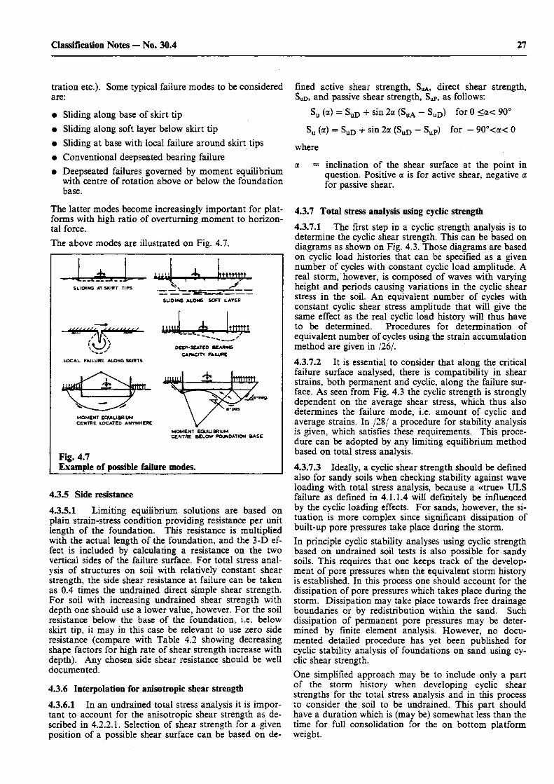
27 Classification Notes — No. 30.4
tration etc.). Some typical failure modes to be considered are:
• Sliding along base of skirt tip • Sliding along soft layer below skirt tip • Sliding at base with local failure around skirt tips • Conventional deepseated bearing failure • Deepseated failures governed by moment equilibrium
with centre of rotation above or below the foundation base.
The latter modes become increasingly important for plat-forms with high ratio of overturning moment to horizon-tal force. The above modes are illustrated on Fig. 4.7.
SLIDING AT SKIRT TIPS
ttump.,
SLIDING ALONG SOFT LAYER
LOCAL FAILURE ALONG SKIRTS
M I SAGA.
DCEP-SEATEO BEARING
CAPACITY FAILURE
MOMENT EQUILIBRIUM CENTRE LOCATED ANYWHERE
MOMENT EQUILIBRIUM CENTRE BELOW FOUNDATION B A S E
Fig. 4.7 Example of possible failure modes.
4.3.5 Side resistance
4.3.5.1 Limiting equilibrium solutions are based on plain strain-stress condition providing resistance per unit length of the foundation. This resistance is multiplied with the actual length of the foundation, and the 3-D ef-fect is included by calculating a resistance on the two vertical sides of the failure surface. For total stress anal-ysis of structures on soil with relatively constant shear strength, the side shear resistance at failure can be taken as 0.4 times the undrained direct simple shear strength. For soil with increasing undrained shear strength with depth one should use a lower value, however. For the soil resistance below the base of the foundation, i.e. below skirt tip, it may in this case be relevant to use zero side resistance (compare with Table 4.2 showing decreasing shape factors for high rate of shear strength increase with depth). Any chosen side shear resistance should be well documented.
4.3.6 Interpolation for anisotropic shear strength
4.3.6.1 In an undrained total stress analysis it is impor-tant to account for the anisotropic shear strength as de-scribed in 4.2.2.1. Selection of shear strength for a given position of a possible shear surface can be based on de-
fined active shear strength, Sua, direct shear strength, SUD> and passive shear strength, Sup, as follows:
Su (a) = Su D + sin 2a (SuA - SuD) for 0 <a< 90°
Su (a) = Su D 4- sin 2a (SuD - SuP) for - 90°<a< 0
where
a = inclination of the shear surface at the point in question. Positive a is for active shear, negative a for passive shear.
4.3.7 Total stress analysis using cyclic strength
4.3.7.1 The first step in a cyclic strength analysis is to determine the cyclic shear strength. This can be based on diagrams as shown on Fig. 4.3. Those diagrams are based on cyclic load histories that can be specified as a given number of cycles with constant cyclic load amplitude. A real storm, however, is composed of waves with varying height and periods causing variations in the cyclic shear stress in the soil. An equivalent number of cycles with constant cyclic shear stress amplitude that will give the same effect as the real cyclic load history will thus have to be determined. Procedures for determination of equivalent number of cycles using the strain accumulation method are given in /26/.
4.3.7.2 It is essential to consider that along the critical failure surface analysed, there is compatibility in shear strains, both permanent and cyclic, along the failure sur-face. As seen from Fig. 4.3 the cyclic strength is strongly dependent on the average shear stress, which thus also determines the failure mode, i.e. amount of cyclic and average strains. In /28/ a procedure for stability analysis is given, which satisfies these requirements. This proce-dure can be adopted by any limiting equilibrium method based on total stress analysis.
4.3.7.3 Ideally, a cyclic shear strength should be defined also for sandy soils when checking stability against wave loading with total stress analysis, because a «true» ULS failure as defined in 4.1.1.4 will definitely be influenced by the cyclic loading effects. For sands, however, the si-tuation is more complex since significant dissipation of built-up pore pressures take place during the storm. In principle cyclic stability analyses using cyclic strength based on undrained soil tests is also possible for sandy soils. This requires that one keeps track of the develop-ment of pore pressures when the equivalent storm history is established. In this process one should account for the dissipation of pore pressures which takes place during the storm. Dissipation may take place towards free drainage boundaries or by redistribution within the sand. Such dissipation of permanent pore pressures may be deter-mined by finite element analysis. However, no docu-mented detailed procedure has yet been published for cyclic stability analysis of foundations on sand using cy-clic shear strength. One simplified approach may be to include only a part of the storm history when developing cyclic shear strengths for the total stress analysis and in this process to consider the soil to be undrained. This part should have a duration which is (may be) somewhat less than the time for full consolidation for the on bottom platform weight.
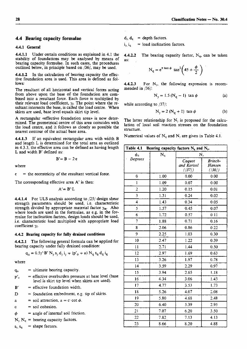
28 Classification Notes — No. 30.4
4.4 Bearing capacity formulae 4.4.1 General
4.4.1.1 Under certain conditions as explained in 4.1 the stability of foundations may be analysed by means of bearing capacity formulae. In such cases, the procedures outlined below, in principle based on /36/, may be used.
4.4.1.2 In the calculation of bearing capacity the effec-tive foundation area is used. This area is defined as fol-lows: The resultant of all horizontal and vertical forces acting from above upon the base of the foundation are com-bined into a resultant force. Each force is multiplied by their relevant load coefficient, The point where the re-sultant intersects the base, is called the load centre. When skirts are used, base level equals skirt tip level. A rectangular «effective foundation area» is now deter-mined. The geometrical centre of this area coincides with the load centre, and it follows as closely as possible the nearest contour of the actual base area.
4.4.1.3 If an equivalent rectangular area with width B and length L is determined for the total area as outlined in 4.3.3, the effective area can be defined as having length L and width B' defined as:
B'= B - 2-e
where
e = the eccentricity of the resultant vertical force.
The corresponding effective area A' is then: A'= B'-L
4.4.1.4 For ULS analysis according to /25/ design shear strength parameters should be used, i.e. characteristic strength divided by appropriate material factor ym. Also where loads are used in the formulae, as e.g. in the for-mulae for inclination factors, design loads should be used, i.e. characteristic load multiplied with appropriate load coefficient yr.
4.4.2 Bearing capacity for fully drained conditions
4.4.2.1 The following general formula can be applied for bearing capacity under fully drained condition:
qu = 0 .5 /B ' Ny Sy dy iy + (p'0 + a) Nq sq dq iq
where
qu = ultimate bearing capacity. p'0 = effective overburden pressure at base level (base
level is skirt tip level when skirts are used). B' = effective foundation width. D = foundation embedment, e.g. tip of skirts. a = soil attraction, a = c- cot <f>. c = soil cohesion. <f> = angle of internal soil friction. Ny, Nq = bearing capacity factors. Sy. sq = shape factors.
dy? dq = depth factors. iv, iq = load inclination factors.
4.4.2.2 The bearing capacity factor, Nq, can be taken as:
Nq = eKtan<f' t a n ^ 4 5 + _ ^
4.4.2.3 For Ny, the following expression is recom-mended in /36/:
Ny = 1.5 (Nq — 1) tan <t> (a)
while according to /37/:
Ny = 2(N q + l) tan cj> (b)
The latter relationship for N7 is proposed for the calcu-lation of local soil reaction stresses on the foundation structure. Numerical values of Nq and Ny are given in Table 4.1.
Table 4.1 Bearing capacity factors N, and N r
<£d Degrees
Nq Ny <£d Degrees
Nq
Caquot and Kerisel
(1371)
Brinch-Hansen (1361)
0 1.00 0.00 0.00 1 1.09 0.07 0.00 2 1.20 0.15 0.01 3 1.31 0.24 0.02 4 1.43 0.34 0.05 5 1.57 0.45 0.07 6 1.72 0.57 Oi l 7 1.88 0.71 0.16 8 2.06 0.86 0.22 9 2.25 1.03 0.30 10 2.47 1.22 0.39 11 2.71 1.44 0.50 12 2.97 1.69 0.63 13 3.26 1.97 0.78 14 3.59 2.29 0.97 15 3.94 2.65 ! .18 16 4.34 3.06 1.43 17 4.77 3.53 1.73 18 5.26 4.07 2.08 19 5.80 4.68 2.48 20 6.40 5.39 2.95 21 7.07 6.20 3.50 22 7.82 7.13 4.13 23 8.66 8.20 4.88
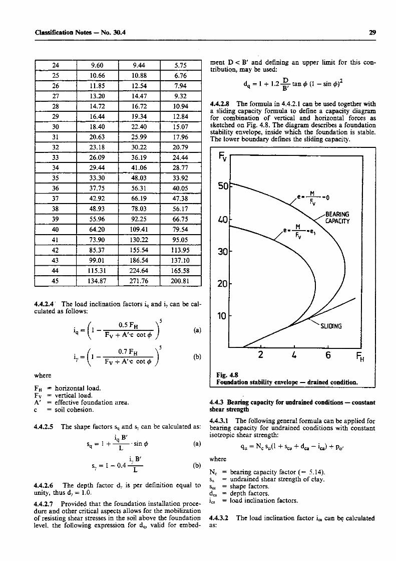
29 Classification Notes — No. 30.4
24 9.60 9.44 5.75 25 10.66 10.88 6.76 26 11.85 12.54 7.94 27 13.20 14.47 9.32 28 14.72 16.72 10.94 29 16.44 19.34 12.84 30 18.40 22.40 15.07 31 20.63 25.99 17.96 32 23.18 30.22 20.79 33 26.09 36.19 24.44 34 29.44 41.06 28.77 35 33.30 48.03 33.92 36 37.75 56.31 40.05 37 42.92 66.19 47.38 38 48.93 78.03 56.17 39 55.96 92.25 66.75 40 64.20 109.41 79.54 41 73.90 130.22 95.05 42 85.37 155.54 113.95 43 99.01 186.54 137.10 44 115.31 224.64 165.58 45 134.87 271.76 200.81
4.4.2.4 The load inclination factors iq and ir can be cal-culated as follows:
_ / 0.5 F H \ 5
- [ l ~ F v + A' c cot (p ) ( a )
/ 0.7 F h \ 5
ly = \ ~ F v t A'-c cot (f> ) ( b )
where
F h = horizontal load. FV ~ vertical load. A' = effective foundation area, c = soil cohesion.
4.4.2.5 The shape factors sq and s? can be calculated as:
iq B'
sq = 1 + —j— • sin 4> (a)
LB' sv = 1 — 0.4 — — (b) > L
4.4.2.6 The depth factor dv is per definition equal to unity, thus d? = 1.0. 4.4.2.7 Provided that the foundation installation proce-dure and other critical aspects allows for the mobilization of resisting shear stresses in the soil above the foundation level, the following expression for dq, valid for embed-
ment D < B' and defining an upper limit for this con-tribution, may be used:
dq = 1 + 1.2-|5-tan 0(1 -sin<£)2 4 B
4.4.2.8 The formula in 4.4.2.1 can be used together with a sliding capacity formula to define a capacity diagram for combination of vertical and horizontal forces as sketched on Fig. 4.8. The diagram describes a foundation stability envelope, inside which the foundation is stable. The lower boundary defines the sliding capacity.
Fig. 4.8 Foundation stability envelope — drained condition.
4.4.3 Bearing capacity for undrained conditions — constant shear strength
4.4.3.1 The following general formula can be applied for bearing capacity for undrained conditions with constant isotropic shear strength:
Qu = Nc su(l + sca + d^ - i^) + pc,
where
Nc = bearing capacity factor (= 5.14). su = undrained shear strength of clay. Sca = shape factors. dca = depth factors. ica = load inclination factors.
4.4.3.2 The load inclination factor ica can be calculated as:
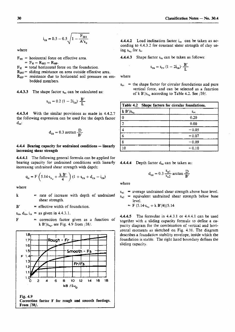
30 Classification Notes — No. 30.4
where
FHI = horizontal force on effective area. = F H — R H O ~ RHP-
Fh = total horizontal force on the foundation. RHO = sliding resistance on area outside effective area. RHP = resistance due to horizontal soil pressure on em-
bedded members.
4.4.3.3 The shape factor Sea can be calculated as:
sca = 0.2 (1 — 2ica)-
4.4.3.4 With the similar provisions as made in 4.4.2.7 the following expression can be used for the depth factor dca :
dca = 0.3 arctan
4.4.4 Bearing capacity for undrained conditions — linearly increasing shear strength
4.4.4.1 The following general formula can be applied for bearing capacity for undrained conditions with linearly increasing undrained shear strength with depth:
qu = F (5.14-sUo + ) (1 + sca + dca - ica)
where
k
1 1 nuui yii " r i ~
Sit raoxn - r s raoxn - r s
Fr/Fs
8 10 12 14 16 18 kB /Siu
Fig. 4.9 Correction factor F for rough and smooth footings. From /38/.
4.4.4.2 Load inclination factor ica can be taken as ac-cording to 4.4.3.2 for constant shear strength of clay us-ing sUo for su.
4.4.4.3 Shape factor Sca can be taken as follows:
B' sca ~~ scv (1 ^ca)' T
where
scv = the shape factor for circular foundations and pure vertical force, and can be selected as a function of k B'/sUo according to Table 4.2. See /39/.
Table 4.2 Shape factors for circular foundations. kB'/s„0 Scv
0 0.20 2 0 . 0 0
4 -0 .05 6 -0 .07 8 -0 .09 10 -0.10
4.4.4.4 Depth factor dca can be taken as:
dca = 0.3 -- arctan ca su2 B'
where
= rate of increase with depth of undrained shear strength.
B' = effective width of foundation.
Sca, dca, ica = as given in 4.4.3.1. F = correction factor given as a function of
k B'/Suo, see Fig. 4.9 from /38/.
sui = average undrained shear strength above base level. su2 = equivalent undrained shear strength below base
level. = F(5.14-sUo + kB'/4)/5.14
4.4.4.5 The formulae in 4.4.3.1 or 4.4.4.1 can be used together with a sliding capacity formula to define a ca-pacity diagram for the combination of vertical and hori-zontal moments as sketched on Fig. 4.10. The diagram describes a foundation stability envelope, inside which the foundation is stable. The right hand boundary defines the sliding capacity.
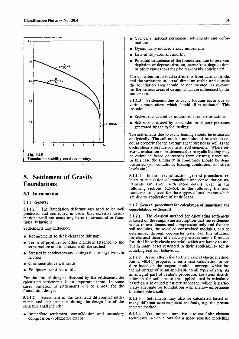
31 Classification Notes — No. 30.4
p. rv
40
30
20
10 ^SLIDING
1 2 3 4 5 6 Fh
Fig. 4.10 Foundation stability envelope — clay.
5. Settlement of Gravity Foundations 5.1 Introduction 5.1.1 General
5.1.1.1 The foundation deformations need to be well predicted and controlled in order that excessive defor-mations shall not cause any harm to structural or func-tional behaviour. Settlements may influence:
• Requirements to deck clearance (air gap) • Tie-in of pipelines or other members attached to the
substructure and in contact with the seabed • Stresses in conductors and casings due to negative skin
friction • Clearance above wellheads • Equipment sensitive to tilt.
For the area of design influenced by the settlements the calculated settlements is an important input. In some cases limitation of settlements will be a goal for the foundation design.
5.1.1.2 Assessment of the total and differential settle-ments and displacements during the design life of the structure shall include:
• Immediate settlement, consolidation and secondary compression (volumetric creep)
• Cyclically induced permanent settlements and defor-mations
• Dynamically induced elastic movements • Lateral displacement and tilt • Potential subsidence of the foundation due to reservoir
depletion or depressurization, permafrost degradation, or other causes that may be reasonably anticipated.
The contribution to total settlements from various depths and the variations in lateral direction within and outside the foundation area should be documented, as relevant for the various areas of design which are influenced by the settlements.
5.1.1.3 Settlements due to cyclic loading occur due to various mechanisms, which should all be evaluated. This includes:
• Settlements caused by undrained shear deformations • Settlements caused by consolidation of pore pressures
generated by the cyclic loading.
The settlements due to cyclic loading should be estimated analytically. The soil models used should be able to ac-count properly for the average shear stresses as well as the cyclic shear stress history in all soil elements. Where rel-evant, evaluation of settlements due to cyclic loading may be estimated based on records from existing structures. In this case the similarity in conditions should be dem-onstrated (soil conditions, loading conditions, soil stress levels etc.).
5.1.1.4 In the next subsection, general procedures re-lated to calculation of immediate and consolidation set-tlements are given, with more details given in the following sections, 5.2—5.4. In the following the term «settlement» is used for these types of settlements which are due to application of static loads.
5.1.2 General procedures for calculation of immediate and consolidation settlements 5.1.2.1 The classical method for calculating settlement is based on the simplifying assumption that the settlement is due to one-dimensional compression only and that the soil modulus, the so-called constrained modulus, can be determined through oedometer tests. For this situation the classical theory of elasticity provides simple formulae for ideal linearly elastic material, which are handy to use, but in many cases restricted in their applicability for si-mulating real soil behaviour.
5.1.2.2 As an alternative to the classical elastic method, Janbu /40,41/ proposed a settlement calculation proce-dure based on the tangent modulus concept, which has the advantage of being applicable to all types of soils. As an integral part of Janbu's procedure, the stress distrib-ution in the soil due to the applied load is calculated based on a so-called plasticity approach, which is partic-ularly adequate for foundations wixh shallow embedment in cohesionless soils.
5.1.2.3 Settlements may also be calculated based on many different semi-empirical methods, e.g. the pressu-remeter method.
5.1.2.4 Yet another alternative is to use finite element techniques, which allows for a more realistic modelling
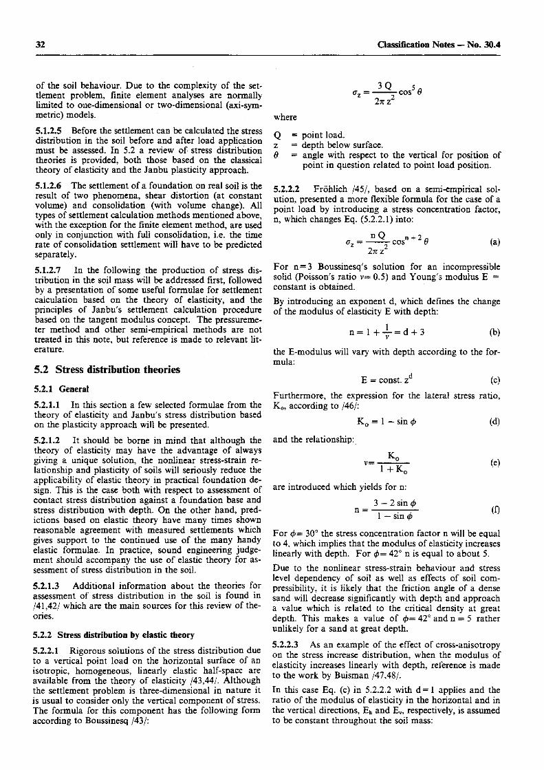
32 Classification Notes — No. 30.4
of the soil behaviour. Due to the complexity of the set-tlement problem, finite element analyses are normally limited to one-dimensional or two-dimensional (axi-sym-metric) models.
5.1.2.5 Before the settlement can be calculated the stress distribution in the soil before and after load application must be assessed. In 5.2 a review of stress distribution theories is provided, both those based on the classical theory of elasticity and the Janbu plasticity approach.
5.1.2.6 The settlement of a foundation on real soil is the result of two phenomena, shear distortion (at constant volume) and consolidation (with volume change). All types of settlement calculation methods mentioned above, with the exception for the finite element method, are used only in conjunction with full consolidation, i.e. the time rate of consolidation settlement will have to be predicted separately.
5.1.2.7 In the following the production of stress dis-tribution in the soil mass will be addressed first, followed by a presentation of some useful formulae for settlement calculation based on the theory of elasticity, and the principles of Janbu's settlement calculation procedure based on the tangent modulus concept. The pressureme-ter method and other semi-empirical methods are not treated in this note, but reference is made to relevant lit-erature.
5.2 Stress distribution theories 5.2.1 General
5.2.1.1 In this section a few selected formulae from the theory of elasticity and Janbu's stress distribution based on the plasticity approach will be presented.
5.2.1.2 It should be borne in mind that although the theory of elasticity may have the advantage of always giving a unique solution, the nonlinear stress-strain re-lationship and plasticity of soils will seriously reduce the applicability of elastic theory in practical foundation de-sign. This is the case both with respect to assessment of contact stress distribution against a foundation base and stress distribution with depth. On the other hand, pred-ictions based on elastic theory have many times shown reasonable agreement with measured settlements which gives support to the continued use of the many handy elastic formulae. In practice, sound engineering judge-ment should accompany the use of elastic theory for as-sessment of stress distribution in the soil.
5.2.1.3 Additional information about the theories for assessment of stress distribution in the soil is found in /41,42/ which are the main sources for this review of the-ories.
5.2.2 Stress distribution by elastic theory
5.2.2.1 Rigorous solutions of the stress distribution due to a vertical point load on the horizontal surface of an isotropic, homogeneous, linearly elastic half-space are available from the theory of elasticity /43,44/. Although the settlement problem is three-dimensional in nature it is usual to consider only the vertical component of stress. The formula for this component has the following form according to Boussinesq /43/:
l ^ C O S 5 * In z
where
Q = point load, z = depth below surface. 0 = angle with respect to the vertical for position of
point in question related to point load position.
5.2.2.2 Frohlich /45/, based on a semi-empirical sol-ution, presented a more flexible formula for the case of a point load by introducing a stress concentration factor, n, which changes Eq. (5.2.2.1) into:
az = —— r̂- cosn + ^ 6 2n z
(a)
For n = 3 Boussinesq's solution for an incompressible solid (Poisson's ratio v= 0.5) and Young's modulus E = constant is obtained. By introducing an exponent d, which defines the change of the modulus of elasticity E with depth:
n = 1 + i - = d + 3 (b)
the E-modulus will vary with depth according to the for-mula:
E = const. zd (c) Furthermore, the expression for the lateral stress ratio, K0, according to /46/:
K0 = 1 — sin <f)
and the relationship:
1 + K n
are introduced which yields for n:
3 — 2 sin </> n = •
1 — sin <j>
(d)
(e)
(0
For </>= 30° the stress concentration factor n will be equal to 4, which implies that the modulus of elasticity increases linearly with depth. For <t>= 42° n is equal to about 5. Due to the nonlinear stress-strain behaviour and stress level dependency of soil as well as effects of soil com-pressibility, it is likely that the friction angle of a dense sand will decrease significantly with depth and approach a value which is related to the critical density at great depth. This makes a value of (j)= 42° and n = 5 rather unlikely for a sand at great depth.
5.2.2.3 As an example of the effect of cross-anisotropy on the stress increase distribution, when the modulus of elasticity increases linearly with depth, reference is made to the work by Buisman /47,48/. In this case Eq. (c) in 5.2.2.2 with d = 1 applies and the ratio of the modulus of elasticity in the horizontal and in the vertical directions, Eh and Ev, respectively, is assumed to be constant throughout the soil mass:
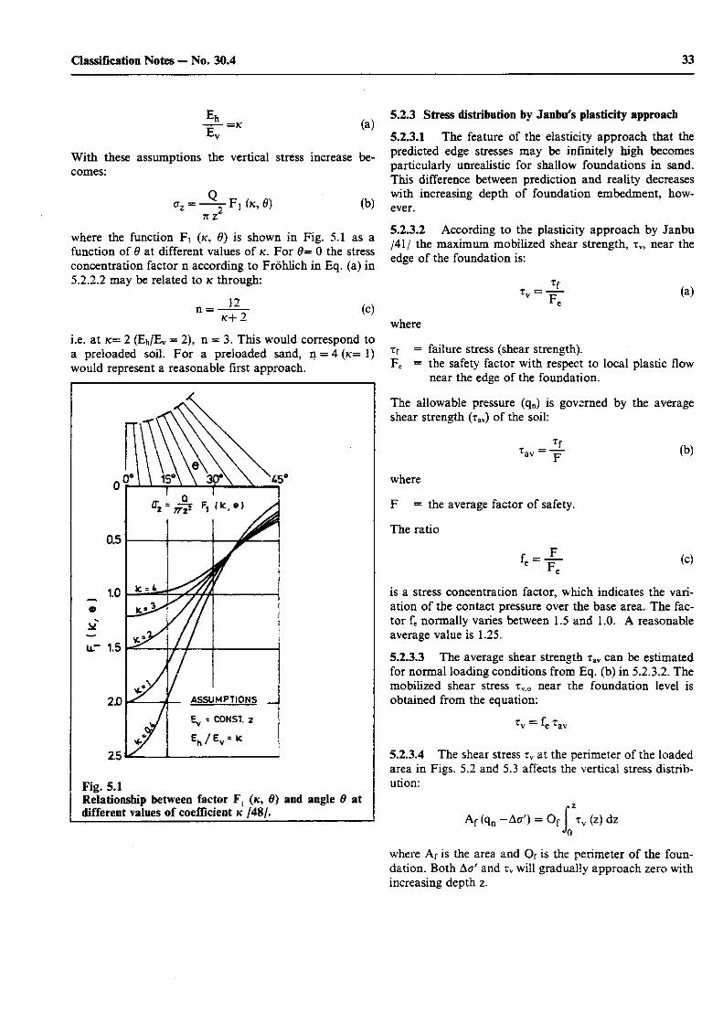
33 Classification Notes — No. 30.4
= 7 C (a)
With these assumptions the vertical stress increase be-comes:
< t z = — 6 ) 71 Z
(b)
where the function Fi (k, 9) is shown in Fig. 5.1 as a function of 9 at different values of K. For 0= 0 the stress concentration factor n according to Frohlich in Eq. (a) in 5.2.2.2 may be related to K through:
n = 12 2
0.5
10
LIT 1.5
2.0
2.5
' ' 1 !1V 7TZ1 P1 —
/! . ASSL IMPTIONS _ A Ey = CONST. 2
j
Fig. 5.1 Relationship between factor F{ (k, 0) and angle 9 at different values of coefficient K /48/.
5.2.3 Stress distribution by Janbu's plasticity approach
5.2.3.1 The feature of the elasticity approach that the predicted edge stresses may be infinitely high becomes particularly unrealistic for shallow foundations in sand. This difference between prediction and reality decreases with increasing depth of foundation embedment, how-ever.
5.2.3.2 According to the plasticity approach by Janbu /41/ the maximum mobilized shear strength, Tv, near the edge of the foundation is:
(c) (a)
where i.e. at K— 2 (Eh/Ev = 2), n = 3. This would correspond to a preloaded soil. For a preloaded sand, n = 4( /c=l) would represent a reasonable first approach.
Tf = failure stress (shear strength). Fe = the safety factor with respect to local plastic flow
near the edge of the foundation.
The allowable pressure (qn) is governed by the average shear strength (tav) of the soil:
T a v - p (b)
where
F = the average factor of safety.
The ratio
f — e Fe (c)
is a stress concentration factor, which indicates the vari-ation of the contact pressure over the base area. The fac-tor fc normally varies between 1.5 and 1.0. A reasonable average value is 1.25.
5.2.3.3 The average shear strength iav can be estimated for normal loading conditions from Eq. (b) in 5.2.3.2. The mobilized shear stress Tv,0 near the foundation level is obtained from the equation:
T = f T L\ Ae lav
5.2.3.4 The shear stress Tv at the perimeter of the loaded area in Figs. 5.2 and 5.3 affects the vertical stress distrib-ution:
Af(q, n -Aa ' ) = Of f Jo
T v (z) dz
where Af is the area and Of is the perimeter of the foun-dation. Both A & and iv will gradually approach zero with increasing depth z.
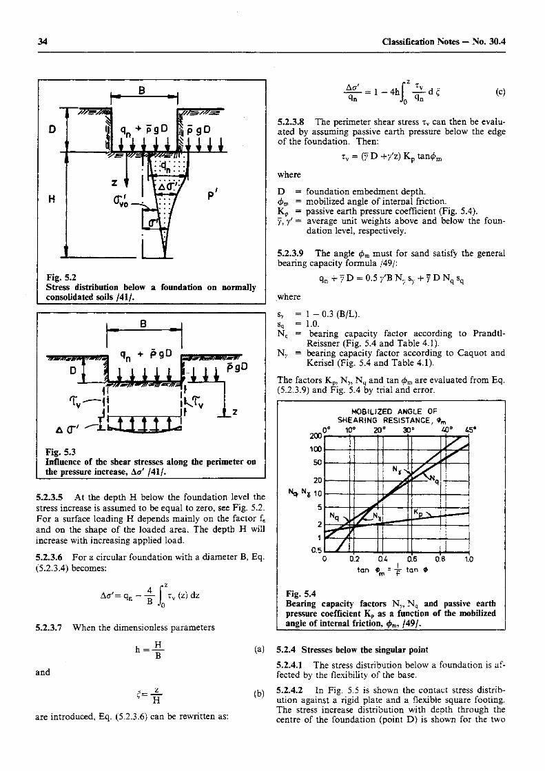
34 Classification Notes — No. 30.4
H
Fig. 5.2 Stress distribution below a foundation on normally consolidated soils /41/.
B
T l u •1 •11 •1P9D
TV (z) dz
5.2.3.7 When the dimensionless parameters
h H
"B"
and
c= z H
(a)
(b)
are introduced, Eq. (5.2.3.6) can be rewritten as:
In Jn <ln (c)
5.2.3.8 The perimeter shear stress Tv can then be evalu-ated by assuming passive earth pressure below the edge of the foundation. Then:
Tv = (y D +y'z) Kp tan<£n
where
D = foundation embedment depth. 4>m = mobilized angle of internal friction. Kp = passive earth pressure coefficient (Fig. 5.4). y, y' = average unit weights above and below the foun-
dation level, respectively.
5.2.3.9 The angle (j>m must for sand satisfy the general bearing capacity formula /49/:
qn + 7D = 0 . 5 / B N 7 s 7 + y D N q s q
where
Sy = 1 - 0.3 (B/L). Sq = 1.0. Nq = bearing capacity factor according to Prandtl-
Reissner (Fig. 5.4 and Table 4.1). N7 = bearing capacity factor according to Caquot and
Kerisel (Fig. 5.4 and Table 4.1).
The factors Kp, N7, Nq and tan <£m are evaluated from Eq. (5.2.3.9) and Fig. 5.4 by trial and error.
Fig. 5.3 Influence of the shear stresses along the perimeter on the pressure increase, &<r' /41/.
5.2.3.5 At the depth H below the foundation level the stress increase is assumed to be equal to zero, see Fig. 5.2. For a surface loading H depends mainly on the factor fe and on the shape of the loaded area. The depth H will increase with increasing applied load.
5.2.3.6 For a circular foundation with a diameter B, Eq. (5.2.3.4) becomes:
200
100 50
20 N̂ 10
5
2 1
0.5
MOBILIZED ANGLE OF SHEARING RESISTANCE, <TM
0° 10° 20° 30° 40° £5°
0.2 (H
i * Q 1 f
J i
X KD
X
p 1 0.6 0.8 1.0
tan * - -r tan 0 m r
Fig. 5.4 Bearing capacity factors N7, Nq and passive earth pressure coefficient Kp as a function of the mobilized angle of internal friction, /49/.
5.2.4 Stresses below the singular point 5.2.4.1 The stress distribution below a foundation is af-fected by the flexibility of the base.
5.2.4.2 In Fig. 5.5 is shown the contact stress distrib-ution against a rigid plate and a flexible square footing. The stress increase distribution with depth through the centre of the foundation (point D) is shown for the two
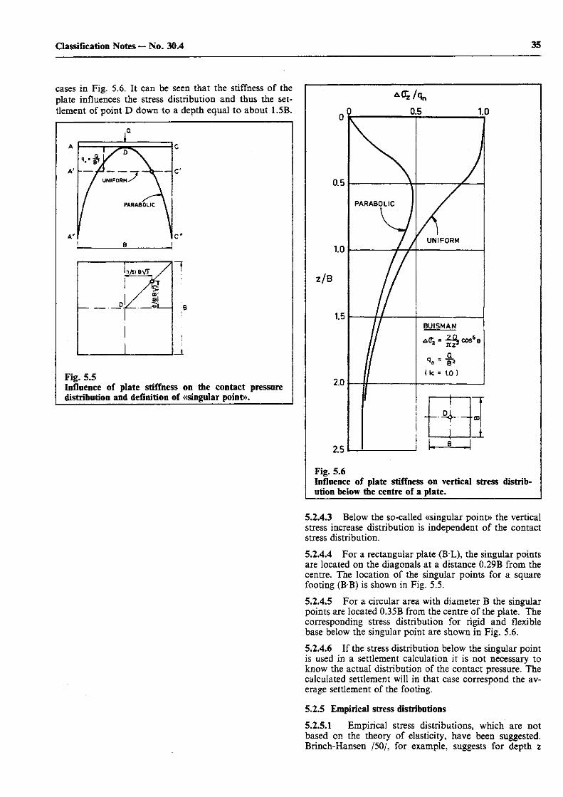
35 Classification Notes — No. 30.4
cases in Fig. 5.6. It can be seen that the stiffness of the plate influences the stress distribution and thus the set-tlement of point D down to a depth equal to about 1.5B.
Fig. 5.5 Influence of plate stiffness on the contact pressure distribution and definition of «singular point».
2.5
(k = 10 )
1
i
•CD
, B
Fig. 5.6 Influence of plate stiffness on vertical stress distrib-ution below the centre of a plate.
5.2.4.3 Below the so-called «singular point» the vertical stress increase distribution is independent of the contact stress distribution.
5.2.4.4 For a rectangular plate (BL), the singular points are located on the diagonals at a distance 0.29B from the centre. The location of the singular points for a square footing (B B) is shown in Fig. 5.5.
5.2.4.5 For a circular area with diameter B the singular points are located 0.35B from the centre of the plate. The corresponding stress distribution for rigid and flexible base below the singular point are shown in Fig. 5.6.
5.2.4.6 If the stress distribution below the singular point is used in a settlement calculation it is not necessary to know the actual distribution of the contact pressure. The calculated settlement will in that case correspond the av-erage settlement of the footing.
5.2.5 Empirical stress distributions
5.2.5.1 Empirical stress distributions, which are not based on the theory of elasticity, have been suggested. Brinch-Hansen /50/, for example, suggests for depth z
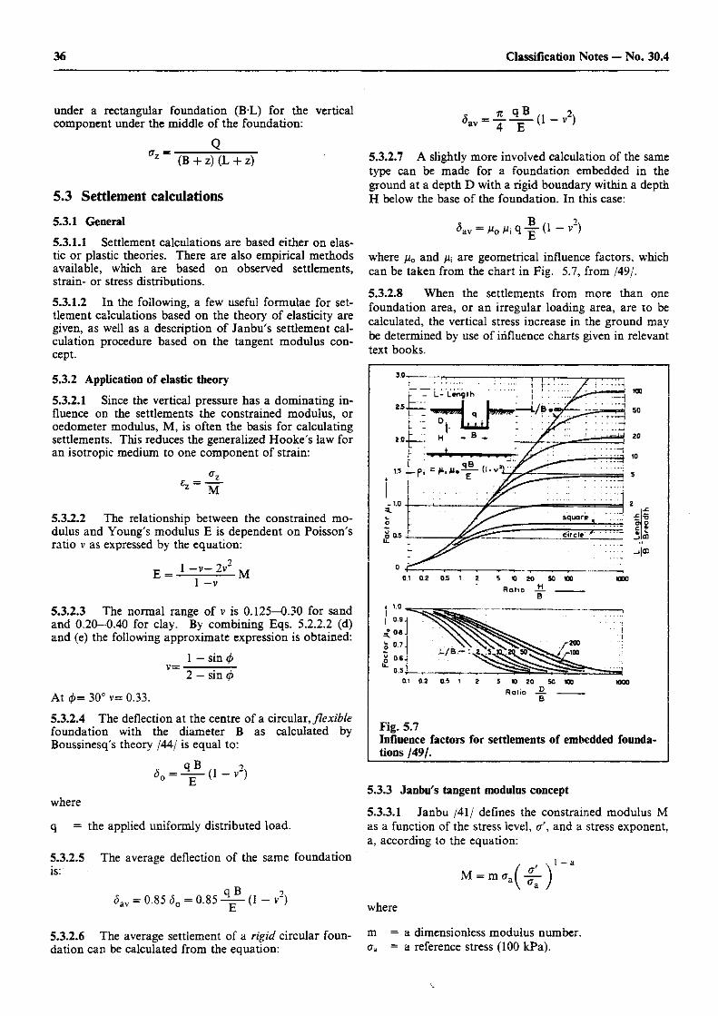
36 Classification Notes — No. 30.4
under a rectangular foundation (B-L) for the vertical component under the middle of the foundation:
Q a z (B + z)(L + z)
5.3 Settlement calculations 5.3.1 General
5.3.1.1 Settlement calculations are based either on elas-tic or plastic theories. There are also empirical methods available, which are based on observed settlements, strain- or stress distributions.
5.3.1.2 In the following, a few useful formulae for set-tlement calculations based on the theory of elasticity are given, as well as a description of Janbu's settlement cal-culation procedure based on the tangent modulus con-cept.
5.3.2 Application of elastic theory
5.3.2.1 Since the vertical pressure has a dominating in-fluence on the settlements the constrained modulus, or oedometer modulus, M, is often the basis for calculating settlements. This reduces the generalized Hooke's law for an isotropic medium to one component of strain:
5.3.2.2 The relationship between the constrained mo-dulus and Young's modulus E is dependent on Poisson's ratio v as expressed by the equation:
E = l ~ v ~ 2 v 2 M 1 —v
5.3.2.3 The normal range of v is 0.125—0.30 for sand and 0.20—0.40 for clay. By combining Eqs. 5.2.2.2 (d) and (e) the following approximate expression is obtained:
_ 1 — sin (j> 2 — sin (f>
At <j)= 30° v= 0.33.
5.3.2.4 The deflection at the centre of a circular, flexible foundation with the diameter B as calculated by Boussinesq's theory /44/ is equal to:
q B ?
Jo-V*1-^ where
q = the applied uniformly distributed load.
5.3.2.5 The average deflection of the same foundation is:
<5av = 0.85 $0 = 0.85 (1 - v 2 )
5.3.2.6 The average settlement of a rigid circular foun-dation can be calculated from the equation:
jj _ 7c q® /, 2\ av T " T i ~ '
5.3.2.7 A slightly more involved calculation of the same type can be made for a foundation embedded in the ground at a depth D with a rigid boundary within a depth H below the base of the foundation. In this case:
B ?
where //0 and fx\ are geometrical influence factors, which can be taken from the chart in Fig. 5.7, from /49/.
5.3.2.8 When the settlements from more than one foundation area, or an irregular loading area, are to be calculated, the vertical stress increase in the ground may be determined by use of influence charts given in relevant text books.
R a t i o - H
0.1 0.2 0.5 1 2 5 10 20 SO 100 1000
R a t i o J L . .
Fig. 5.7 Influence factors for settlements of embedded founda-tions /49/.
5.3.3 Janbu's tangent modulus concept
5.3.3.1 Janbu /41/ defines the constrained modulus M as a function of the stress level, <r', and a stress exponent, a, according to the equation:
M=m<H^r) where
m = a dimensionless modulus number. <xa —a reference stress (100 kPa).
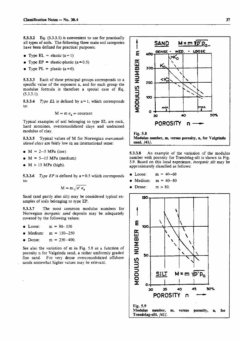
37 Classification Notes — No. 30.4
533.2 Eq. (5.3.3.1) is convenient to use for practically all types of soils. The following three main soil categories have been defined for practical purposes:
• Type EL = elastic (a = 1)
• Type EP = elastic-plastic (a = 0.5)
• Type PL = plastic (a = 0).
5.3.3.3 Each of these principal groups corresponds to a specific value of the exponent a, and for each group the modulus formula is therefore a special case of Eq. (5.3.3.1).
5.3.3.4 to:
M = m <ra = constant
Typical examples of soil belonging to type EL are rock, hard moraines, overconsolidated clays and undrained modulus of clay.
5.3.3.5 Typical values of M for Norwegian overconsol-idated clays are fairly low in an international sense:
• M = 2 - 5 MPa (low)
• M = 5—15 MPa (medium)
• M > 15 MPa (high).
5.3.3.6 Type EP is defined by a = 0.5 which corresponds to:
f S A N D M - m f p ^
& 40Q-
CE ixl CD 300*
Type EL is defined by a = 1, which corresponds
cn
3 D Q O
200
TOO
V \
>
V
\ * \ \ < \ <
\
min. 1.
max 1 _
30 40
P O R O S I T Y n
50%
Fig. 5.8 Modulus number, m, versus porosity, n, for Valgrinda sand, /41/.
M = m^/V a a
Sand (and partly also silt) may be considered typical ex-amples of soils belonging to type EP.
5.3.3.7 The most common modulus numbers for Norwegian inorganic sand deposits may be adequately covered by the following values:
• Loose: m = 80-150
• Medium: m = 150—250
• Dense: m = 250-400.
See also the variation of m in Fig. 5.8 as a function of porosity n for Valgrinda sand, a rather uniformly graded fine sand. For very dense overconsolidated offshore sands somewhat higher values may be relevant.
5.3.3.8 An example of the variation of the modulus number with porosity for Trendelag-silt is shown in Fig. 5.9. Based on this local experience, inorganic silt may be approximately classified as follows:
• Loose: m = 40—60 • Medium: m = 60—80 • Dense: m > 80.
130
TOO* tz 111 m 2
cn 3
Q O 3E
50
\ \
V
k \ \ •A
\ \
>
V \
txj \
S I L r m
L :
\ \
1 :
\
1 30 35 AO 4 5 50T.
P O R O S I T Y n —
Fig. 5.9 Modulus number, m, Trendelag-silt, /41/.
versus porosity, n, for
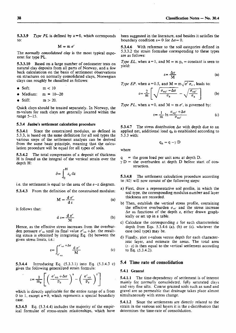
38 Classification Notes — No. 30.4
5.3.3.9 Type PL is defined by a = 0 , which corresponds to:
M = m a '
The normally consolidated clay is the most typical expo-nent for type PL.
5.3.3.10 Based on a large number of oedometer tests on natural clay deposits from all parts of Norway, and a few back calculations on the basis of settlement observations on structures on normally consolidated clays, Norwegian clays can roughly be classified as follows:
• Soft: m < 10 • Medium: m = 10—20 • Stiff: m > 20.
Quick clays should be treated separately. In Norway, the m-values for such clays are generally located within the range 5—15.
5.3.4 Janbu's settlement calculation procedure
5.3.4.1 Since the constrained modulus, as defined in 5.3.3, is based on the same definition for all soil types the various steps of the settlement analysis can be derived from the same basic principle, meaning that the calcu-lation procedure will be equal for all types of soils.
5.3.4.2 The total compression of a deposit of thickness H is found as the integral of the vertical strain over the depth H:
H Jo H
&z dz
i.e. the settlement is equal to the area of the e—z diagram.
5.3.4.3 From the definition of the constrained modulus:
d & M = • d s
it follows that:
d s = d a' M
(a)
(b)
Hence, as the effective stress increases from the overbur-den pressure <j'vo until its final value a \ 0 -fAcr, the result-ing strain is obtained by integrating Eq. (b) between the given stress limits, i.e.:
- I &
been suggested in the literature, and besides it satisfies the boundary condition 0 for Aa= 0.
5.3.4.6 With reference to the soil categories defined in 5.3.3.2 the strain formulae corresponding to these types are as follows: Type EL, when a = 1, and M = m pa = constant is seen to yield:
e= A c t
M
Type EP, when a = 0.5, and M = myjo ' crA, leads to:
2 £ = m
CTV0' +A<7
Type PL, when a = 0, and M = m <j\ is governed by:
1 . * v o ' s= -=- * m Jvor
(a)
(b)
(c)
5.3.4.7 The stress distribution Aa with depth due to an applied net, additional load qn is established according to 5.3.3 with:
qn = q - y D
where
q = the gross load per unit area at depth D. y D = the overburden at depth D before start of con-
struction.
5.3.4.8 The settlement calculation procedure according to 142/ will now consist of the following steps:
a) First, draw a representative soil profile, in which the soil type, the corresponding modulus number and layer thickness are recorded.
b) Then, establish the vertical stress profile, containing the effective overburden ow and the stress increase Ac as functions of the depth z, either drawn graph-ically or set up in a table.
c) Calculate the corresponding c for each characteristic depth from Eqs. 5.3.4.6 (a), (b) or (c). whatever the case (soil type) may be.
d) Finally, plot a-values versus depth for each character-istic layer, and estimate the areas. The total area (e—z) is then equal to the vertical settlement according to Eq. (5.3.4.2).
5.3.4.4 Introducing Eq. (5.3.3.1) into Eq. (5.3.4.3 c) gives the following generalized strain formula:
£ = J _ m *
which is directly applicable for the entire range of a from 0 to 1, except a = 0, which represents a special boundary case.
5.3.4.5 Eq. (5.3.4.4) includes the majority of the empir-ical formulae of stress-strain relationships, which have
5.4 Time rate of consolidation
5.4.1 General
5.4.1.1 The time-dependency of settlement is of interest mainly for normally consolidated, fully saturated clays and very fine silts. Coarse grained soils such as sand and gravel are so permeable that drainage takes place almost simultaneously with stress change.
5.4.1.2 Since the settlements are directly related to the strain in the various soil layers it is the g-distribution that determines the time-rate of consolidation.
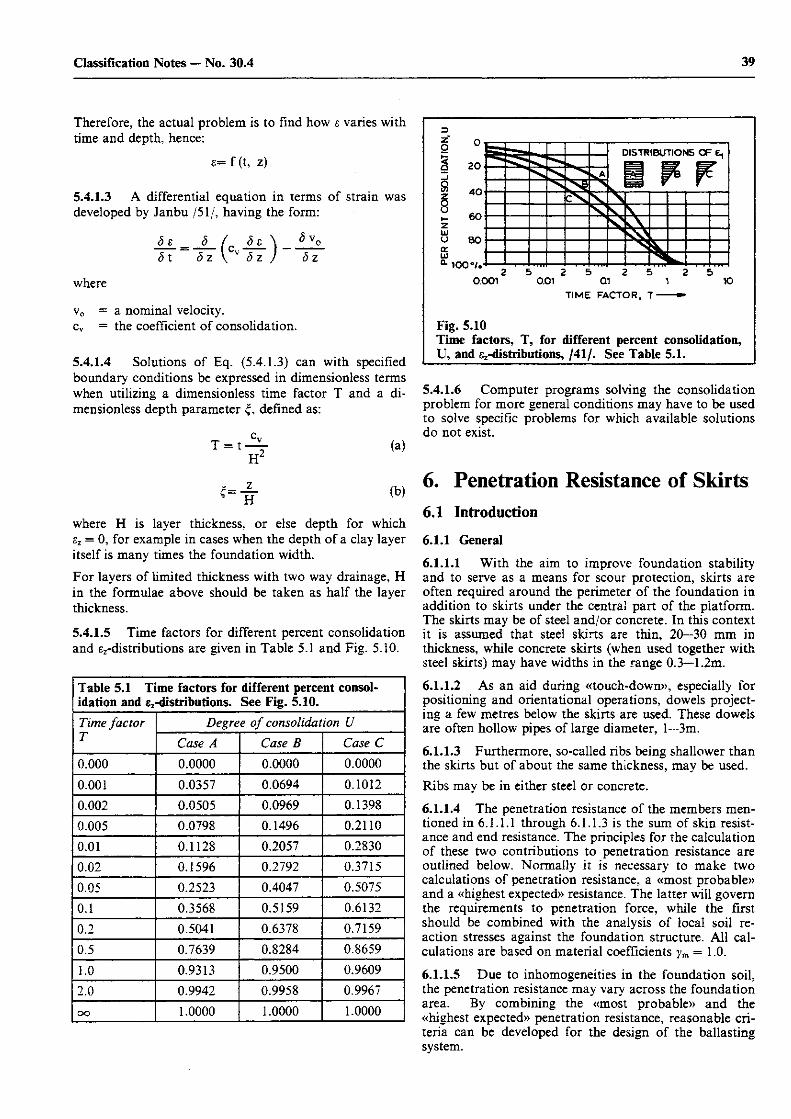
39 Classification Notes — No. 30.4
3 Z 0 1 - J
8 § u H-z Ld U <r UJ CL
0
20
40
60
80
100°/.
DISTRIBUTIONS OF SL
F F SA F F F F
0.001 10 TIME FACTOR, T-
Fig. 5.10 Time factors, T, for different percent consolidation, U, and ^-distributions, /41 /. See Table 5.1.
Therefore, the actual problem is to find how s varies with time and depth, hence:
e= f (t, z)
5.4.1.3 A differential equation in terms of strain was developed by Janbu /51/, having the form:
S e = S f c S e \ < 5 v q
St Sz Sz J S z
where
v0 = a nominal velocity. cv = the coefficient of consolidation.
5.4.1.4 Solutions of Eq. (5.4.1.3) can with specified boundary conditions be expressed in dimensionless terms when utilizing a dimensionless time factor T and a di-mensionless depth parameter defined as:
T = t - \ (a) H 2
where H is layer thickness, or else depth for which £z = 0, for example in cases when the depth of a clay layer itself is many times the foundation width.
For layers of limited thickness with two way drainage, H in the formulae above should be taken as half the layer thickness.
5.4.1.5 Time factors for different percent consolidation and ^-distributions are given in Table 5.1 and Fig. 5.10.
5.4.1.6 Computer programs solving the consolidation problem for more general conditions may have to be used to solve specific problems for which available solutions do not exist.
6. Penetration Resistance of Skirts 6.1 Introduction 6.1.1 General
6.1.1.1 With the aim to improve foundation stability and to serve as a means for scour protection, skirts are often required around the perimeter of the foundation in addition to skirts under the central part of the platform. The skirts may be of steel and/or concrete. In this context it is assumed that steel skirts are thin, 20—30 mm in thickness, while concrete skirts (when used together with steel skirts) may have widths in the range 0.3—1.2m.
6.1.1.2 As an aid during «touch-down», especially for positioning and orientational operations, dowels project-ing a few metres below the skirts are used. These dowels are often hollow pipes of large diameter, 1—3m.
6.1.1.3 Furthermore, so-called ribs being shallower than the skirts but of about the same thickness, may be used. Ribs may be in either steel or concrete.
6.1.1.4 The penetration resistance of the members men-tioned in 6.1.1.1 through 6.1.1.3 is the sum of skin resist-ance and end resistance. The principles for the calculation of these two contributions to penetration resistance are outlined below. Normally it is necessary to make two calculations of penetration resistance, a «most probable» and a «highest expected» resistance. The latter will govern the requirements to penetration force, while the first should be combined with the analysis of local soil re-action stresses against the foundation structure. All cal-culations are based on material coefficients ym = 1.0.
6.1.1.5 Due to inhomogeneities in the foundation soil, the penetration resistance may vary across the foundation area. By combining the «most probable» and the «highest expected» penetration resistance, reasonable cri-teria can be developed for the design of the ballasting system.
Table 5.1 Time factors for different percent consol-idation and ^-distributions. See Fig. 5.10. Time factor T
Degree of consolidation U Time factor T Case A Case B Case C 0.000 0.0000 0.0000 0.0000
0.001 0.0357 0.0694 0.1012 0.002 0.0505 0.0969 0.1398 0.005 0.0798 0.1496 0.2110
0.01 0.1128 0.2057 0.2830 0.02 0.1596 0.2792 0.3715 0.05 0.2523 0.4047 0.5075
0.1 0.3568 0.5159 0.6132
0.2 0.5041 0.6378 0.7159
0.5 0.7639 0.8284 0.8659
1.0 0.9313 0.9500 0.9609
2.0 0.9942 0.9958 0.9967
oo 1.0000 1.0000 1.0000
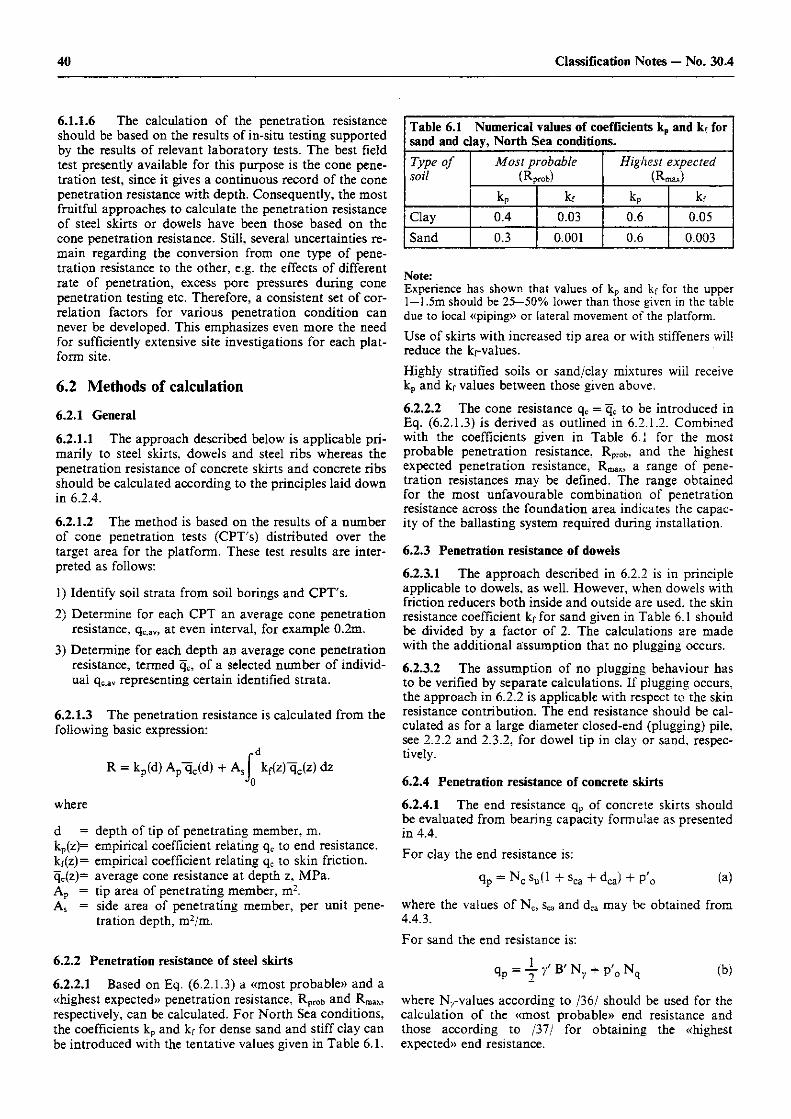
40 Classification Notes — No. 30.4
6.1.1.6 The calculation of the penetration resistance should be based on the results of in-situ testing supported by the results of relevant laboratory tests. The best field test presently available for this purpose is the cone pene-tration test, since it gives a continuous record of the cone penetration resistance with depth. Consequently, the most fruitful approaches to calculate the penetration resistance of steel skirts or dowels have been those based on the cone penetration resistance. Still, several uncertainties re-main regarding the conversion from one type of pene-tration resistance to the other, e.g. the effects of different rate of penetration, excess pore pressures during cone penetration testing etc. Therefore, a consistent set of cor-relation factors for various penetration condition can never be developed. This emphasizes even more the need for sufficiently extensive site investigations for each plat-form site.
6.2 Methods of calculation
6.2.1 General
6.2.1.1 The approach described below is applicable pri-marily to steel skirts, dowels and steel ribs whereas the penetration resistance of concrete skirts and concrete ribs should be calculated according to the principles laid down in 6.2.4.
6.2.1.2 The method is based on the results of a number of cone penetration tests (CPT's) distributed over the target area for the platform. These test results are inter-preted as follows:
1) Identify soil strata from soil borings and CPT's.
2) Determine for each CPT an average cone penetration resistance, qc .av, at even interval, for example 0.2m.
3) Determine for each depth an average cone penetration resistance, termed qc, of a selected number of individ-ual qc,av representing certain identified strata.
6.2.1.3 The penetration resistance is calculated from the following basic expression:
R = kp(d) Ap"qc(d) + As f kKz) qc(z) dz Jo where
d = depth of tip of penetrating member, m. kp(z)= empirical coefficient relating qc to end resistance. kf(z)= empirical coefficient relating qc to skin friction. qc(z)= average cone resistance at depth z, MPa. Ap = tip area of penetrating member, m2. As = side area of penetrating member, per unit pene-
tration depth, m2/m.
6.2.2 Penetration resistance of steel skirts
6.2.2.1 Based on Eq. (6.2.1.3) a «most probable» and a «highest expected» penetration resistance, R p r 0 b and Rm ax ?
respectively, can be calculated. For North Sea conditions, the coefficients kp and kf for dense sand and stiff clay can be introduced with the tentative values given in Table 6.1.
Table 6.1 Numerical values of coefficients kp and kf for sand and clay, North Sea conditions. Type of soil
Most probable (Rprob)
Highest expected (Rmax)
Type of soil
kp kr kp kf
Clay 0 . 4 0 . 0 3 0 . 6 0 . 0 5
Sand 0 . 3 0 . 0 0 1 0 . 6 0 . 0 0 3
Note: Experience has shown that values of kp and kf for the upper 1—1.5m should be 25—50% lower than those given in the table due to local «piping» or lateral movement of the platform. Use of skirts with increased tip area or with stiffeners will reduce the k rvalues. Highly stratified soils or sand/clay mixtures will receive kp and kf values between those given above.
6.2.2.2 The cone resistance qc = qc to be introduced in Eq. (6.2.1.3) is derived as outlined in 6.2.1.2. Combined with the coefficients given in Table 6.1 for the most probable penetration resistance, Rp r 0b, and the highest expected penetration resistance, R m a x , a range of pene-tration resistances may be defined. The range obtained for the most unfavourable combination of penetration resistance across the foundation area indicates the capac-ity of the ballasting system required during installation.
6.2.3 Penetration resistance of dowels
6.2.3.1 The approach described in 6.2.2 is in principle applicable to dowels, as well. However, when dowels with friction reducers both inside and outside are used, the skin resistance coefficient kf for sand given in Table 6.1 should be divided by a factor of 2. The calculations are made with the additional assumption that no plugging occurs.
6.2.3.2 The assumption of no plugging behaviour has to be verified by separate calculations. If plugging occurs, the approach in 6.2.2 is applicable with respect to the skin resistance contribution. The end resistance should be cal-culated as for a large diameter closed-end (plugging) pile, see 2.2.2 and 2.3.2, for dowel tip in clay or sand, respec-tively.
6.2.4 Penetration resistance of concrete skirts
6.2.4.1 The end resistance qp of concrete skirts should be evaluated from bearing capacity formulae as presented in 4.4.
For clay the end resistance is:
Qp = N c s u 0 + s ca + d c a ) + P'o ( a )
where the values of Nc, Sca and dca may be obtained from 4.4.3. For sand the end resistance is:
q p = i - y ' B ' N 7 + p ' 0 N q (b)
where Nv-values according to /36/ should be used for the calculation of the «most probable» end resistance and those according to /37/ for obtaining the «highest expected» end resistance.
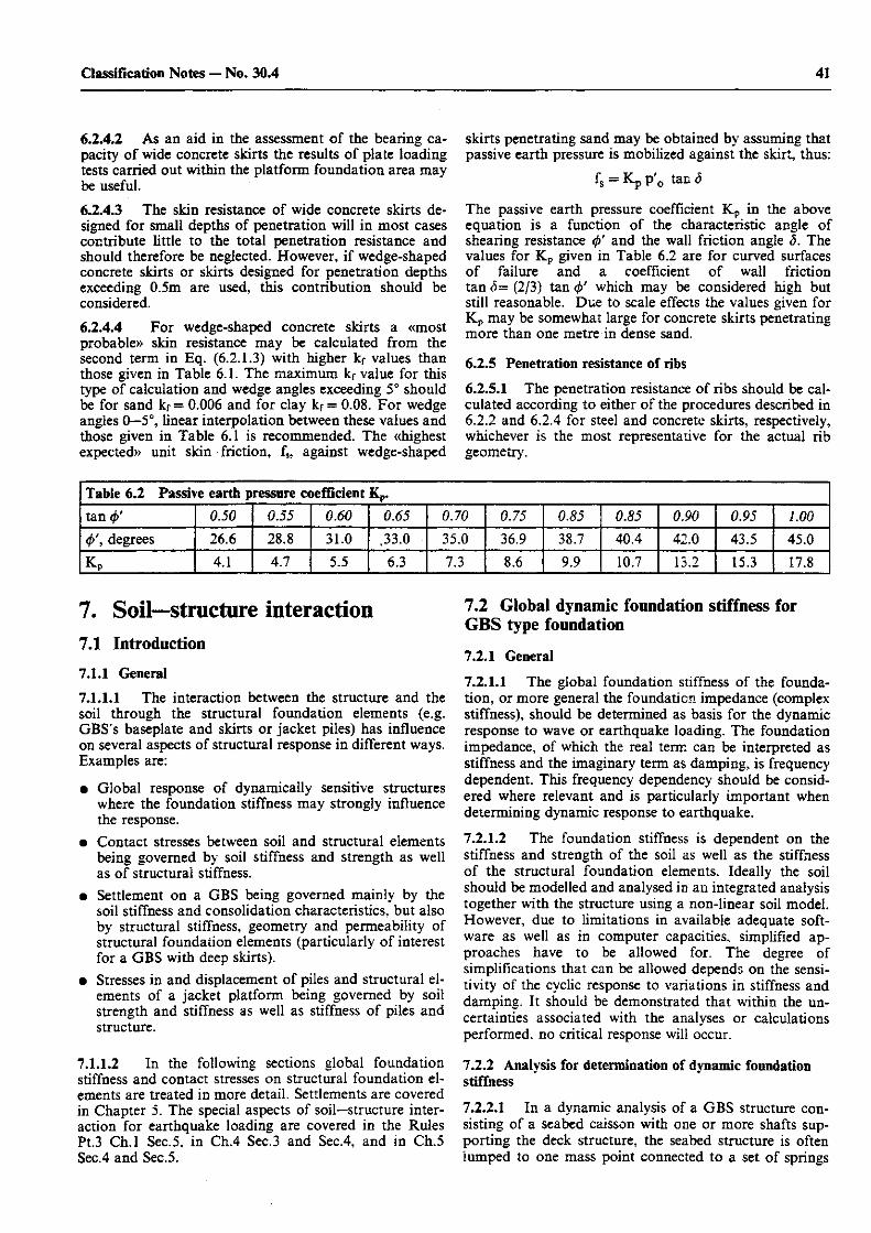
41 Classification Notes — No. 30.4
6.2.4.2 As an aid in the assessment of the bearing ca-pacity of wide concrete skirts the results of plate loading tests carried out within the platform foundation area may be useful. 6.2.4.3 The skin resistance of wide concrete skirts de-signed for small depths of penetration will in most cases contribute little to the total penetration resistance and should therefore be neglected. However, if wedge-shaped concrete skirts or skirts designed for penetration depths exceeding 0.5m are used, this contribution should be considered. 6.2.4.4 For wedge-shaped concrete skirts a «most probable» skin resistance may be calculated from the second term in Eq. (6.2.1.3) with higher kf values than those given in Table 6.1. The maximum kf value for this type of calculation and wedge angles exceeding 5° should be for sand kf = 0.006 and for clay kf = 0.08. For wedge angles 0—5°, linear interpolation between these values and those given in Table 6.1 is recommended. The «highest expected» unit skin friction, fs, against wedge-shaped
7. Soil—structure interaction 7.1 Introduction 7.1.1 General 7.1.1.1 The interaction between the structure and the soil through the structural foundation elements (e.g. GBS s baseplate and skirts or jacket piles) has influence on several aspects of structural response in different ways. Examples are:
• Global response of dynamically sensitive structures where the foundation stiffness may strongly influence the response.
• Contact stresses between soil and structural elements being governed by soil stiffness and strength as well as of structural stiffness.
• Settlement on a GBS being governed mainly by the soil stiffness and consolidation characteristics, but also by structural stiffness, geometry and permeability of structural foundation elements (particularly of interest for a GBS with deep skirts).
• Stresses in and displacement of piles and structural el-ements of a jacket platform being governed by soil strength and stiffness as well as stiffness of piles and structure.
7.1.1.2 In the following sections global foundation stiffness and contact stresses on structural foundation el-ements are treated in more detail. Settlements are covered in Chapter 5. The special aspects of soil—structure inter-action for earthquake loading are covered in the Rules Pt.3 Ch.l Sec.5, in Ch.4 Sec.3 and Sec.4, and in Ch.5 Sec.4 and Sec.5.
skirts penetrating sand may be obtained by assuming that passive earth pressure is mobilized against the skirt, thus:
fs = Kp p'0 tan <5
The passive earth pressure coefficient Kp in the above equation is a function of the characteristic angle of shearing resistance </>' and the wall friction angle S. The values for Kp given in Table 6.2 are for curved surfaces of failure and a coefficient of wall friction tan <5= (2/3) tan 0 ' which may be considered high but still reasonable. Due to scale effects the values given for Kp may be somewhat large for concrete skirts penetrating more than one metre in dense sand.
6.2.5 Penetration resistance of ribs
6.2.5.1 The penetration resistance of ribs should be cal-culated according to either of the procedures described in 6.2.2 and 6.2.4 for steel and concrete skirts, respectively, whichever is the most representative for the actual rib geometry.
7.2 Global dynamic foundation stiffness for GBS type foundation
7.2.1 General
7.2.1.1 The global foundation stiffness of the founda-tion, or more general the foundation impedance (complex stiffness), should be determined as basis for the dynamic response to wave or earthquake loading. The foundation impedance, of which the real term can be interpreted as stiffness and the imaginary term as damping, is frequency dependent. This frequency dependency should be consid-ered where relevant and is particularly important when determining dynamic response to earthquake.
7.2.1.2 The foundation stiffness is dependent on the stiffness and strength of the soil as well as the stiffness of the structural foundation elements. Ideally the soil should be modelled and analysed in an integrated analysis together with the structure using a non-linear soil model. However, due to limitations in available adequate soft-ware as well as in computer capacities, simplified ap-proaches have to be allowed for. The degree of simplifications that can be allowed depends on the sensi-tivity of the cyclic response to variations in stiffness and damping. It should be demonstrated that within the un-certainties associated with the analyses or calculations performed, no critical response will occur.
7.2.2 Analysis for determination of dynamic foundation stiffness
7.2.2.1 In a dynamic analysis of a GBS structure con-sisting of a seabed caisson with one or more shafts sup-porting the deck structure, the seabed structure is often lumped to one mass point connected to a set of springs
Table 6.2 Passive earth pressure coefficient Kp. tan <j>' 0.50 0.55 0.60 0.65 0.70 0.75 0.85 0.85 0.90 0.95 1.00
<f>\ degrees 26.6 28.8 31.0 .33.0 35.0 36.9 38.7 40.4 42.0 43.5 45.0 Kp 4.1 4.7 5.5 6.3 7.3 8.6 9.9 10.7 13.2 15.3 17.8
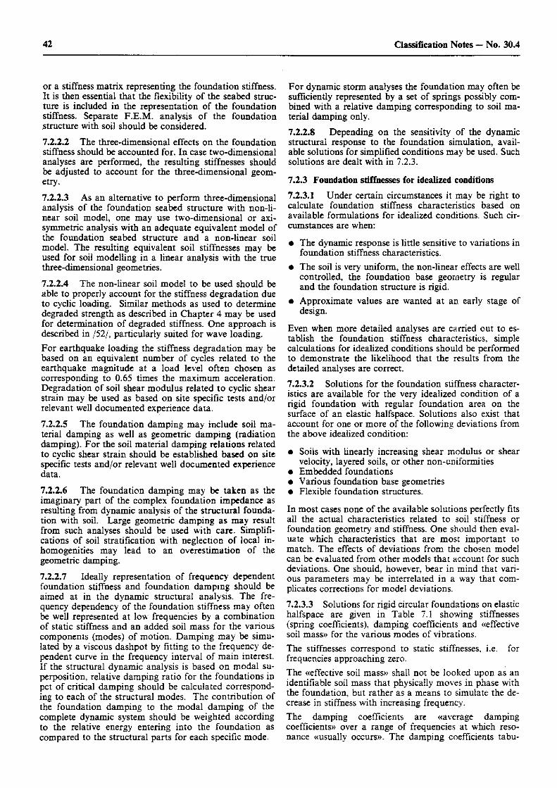
42 Classification Notes — No. 30.4
or a stiffness matrix representing the foundation stiffness. It is then essential that the flexibility of the seabed struc-ture is included in the representation of the foundation stiffness. Separate FJE.M. analysis of the foundation structure with soil should be considered.
7.2.2.2 The three-dimensional effects on the foundation stiffness should be accounted for. In case two-dimensional analyses are performed, the resulting stiffnesses should be adjusted to account for the three-dimensional geom-etry.
7.2.2.3 As an alternative to perform three-dimensional analysis of the foundation seabed structure with non-li-near soil model, one may use two-dimensional or axi-symmetric analysis with an adequate equivalent model of the foundation seabed structure and a non-linear soil model. The resulting equivalent soil stiffnesses may be used for soil modelling in a linear analysis with the true three-dimensional geometries.
7.2.2.4 The non-linear soil model to be used should be able to properly account for the stiffness degradation due to cyclic loading. Similar methods as used to determine degraded strength as described in Chapter 4 may be used for determination of degraded stiffness. One approach is described in /52/, particularly suited for wave loading. For earthquake loading the stiffness degradation may be based on an equivalent number of cycles related to the earthquake magnitude at a load level often chosen as corresponding to 0.65 times the maximum acceleration. Degradation of soil shear modulus related to cyclic shear strain may be used as based on site specific tests and/or relevant well documented experience data.
7.2.2.5 The foundation damping may include soil ma-terial damping as well as geometric damping (radiation damping). For the soil material damping relations related to cyclic shear strain should be established based on site specific tests and/or relevant well documented experience data.
7.2.2.6 The foundation damping may be taken as the imaginary part of the complex foundation impedance as resulting from dynamic analysis of the structural founda-tion with soil. Large geometric damping as may result from such analyses should be used with care. Simplifi-cations of soil stratification with neglection of local in-homogenities may lead to an overestimation of the geometric damping.
7.2.2.7 Ideally representation of frequency dependent foundation stiffness and foundation damping should be aimed at in the dynamic structural analysis. The fre-quency dependency of the foundation stiffness may often be well represented at low frequencies by a combination of static stiffness and an added soil mass for the various components (modes) of motion. Damping may be simu-lated by a viscous dashpot by fitting to the frequency de-pendent curve in the frequency interval of main interest. If the structural dynamic analysis is based on modal su-perposition, relative damping ratio for the foundations in pet of critical damping should be calculated correspond-ing to each of the structural modes. The contribution of the foundation damping to the modal damping of the complete dynamic system should be weighted according to the relative energy entering into the foundation as compared to the structural parts for each specific mode.
For dynamic storm analyses the foundation may often be sufficiently represented by a set of springs possibly com-bined with a relative damping corresponding to soil ma-terial damping only.
7.2.2.8 Depending on the sensitivity of the dynamic structural response to the foundation simulation, avail-able solutions for simplified conditions may be used. Such solutions are dealt with in 7.2.3.
7.2.3 Foundation stiffnesses for idealized conditions 7.2.3.1 Under certain circumstances it may be right to calculate foundation stiffness characteristics based on available formulations for idealized conditions. Such cir-cumstances are when:
• The dynamic response is little sensitive to variations in foundation stiffness characteristics.
• The soil is very uniform, the non-linear effects are well controlled, the foundation base geometry is regular and the foundation structure is rigid.
• Approximate values are wanted at an early stage of design.
Even when more detailed analyses are carried out to es-tablish the foundation stiffness characteristics, simple calculations for idealized conditions should be performed to demonstrate the likelihood that the results from the detailed analyses are correct.
7.2.3.2 Solutions for the foundation stiffness character-istics are available for the very idealized condition of a rigid foundation with regular foundation area on the surface of an elastic halfspace. Solutions also exist that account for one or more of the following deviations from the above idealized condition:
• Soils with linearly increasing shear modulus or shear velocity, layered soils, or other non-uniformities
• Embedded foundations • Various foundation base geometries • Flexible foundation structures.
In most cases none of the available solutions perfectly fits all the actual characteristics related to soil stiffness or foundation geometry and stiffness. One should then eval-uate which characteristics that are most important to match. The effects of deviations from the chosen model can be evaluated from other models that account for such deviations. One should, however, bear in mind that vari-ous parameters may be interrelated in a way that com-plicates corrections for model deviations.
7.2.3.3 Solutions for rigid circular foundations on elastic halfspace are given in Table 7.1 showing stiffnesses (spring coefficients), damping coefficients and «effective soil mass» for the various modes of vibrations. The stiffnesses correspond to static stiffnesses, i.e. for frequencies approaching zero. The «effective soil mass» shall not be looked upon as an identifiable soil mass that physically moves in phase with the foundation, but rather as a means to simulate the de-crease in stiffness with increasing frequency. The damping coefficients are «average damping coefficients» over a range of frequencies at which reso-nance «usually occurs». The damping coefficients tabu-
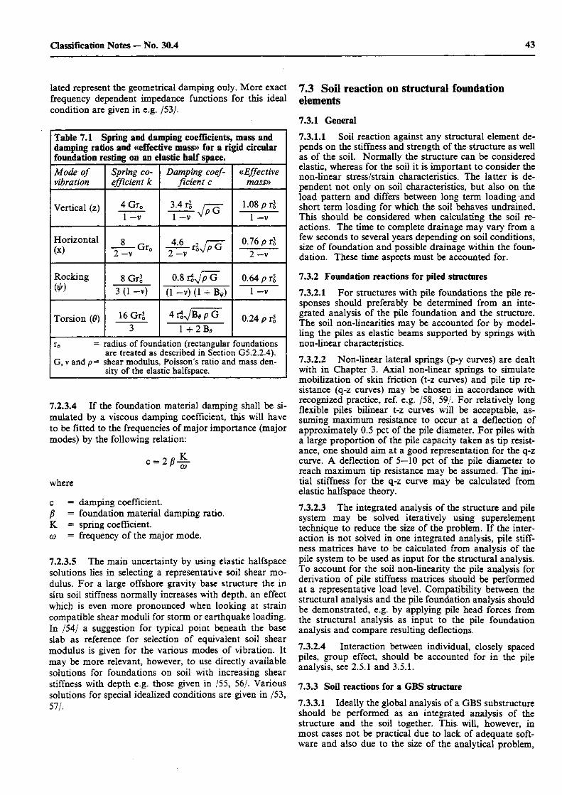
43 Classification Notes — No. 30.4
lated represent the geometrical damping only. More exact frequency dependent impedance functions for this ideal condition are given in e.g. /53/.
Table 7.1 Spring and damping coefficients, mass and damping ratios and «effective mass» for a rigid circular foundation resting on an elastic half space. Mode of vibration
Spring co-efficient k
Damping coef-ficient c
«Effective mass»
Vertical (z) 4 Gr0
1 — V
3.4 xl r-^ 1 - v > G
1.08 pxi 1 - V
Horizontal (x)
8 P r ~ Gr0 2 —v 0.76 p r |
2 - v
Rocking M
8 Grl 0.8 riJp~G 0.64 p 11 Rocking M 3 (1 -v ) (1 -v ) (1 + B,) 1 - V
Torsion (0) 16 Gr£ 3
4 rS^/Bfl p G 1 +2 Be
0.24 p rg
T0 = radius of foundation (rectangular foundations are treated as described in Section G5.2.2.4).
G, v and p= shear modulus, Poisson's ratio and mass den-sity of the elastic halfspace.
7.2.3.4 If the foundation material damping shall be si-mulated by a viscous damping coefficient, this will have to be fitted to the frequencies of major importance (major modes) by the following relation:
c = 2 B — H CO
where
c = damping coefficient. P = foundation material damping ratio. K = spring coefficient. a) = frequency of the major mode.
7.2.3.5 The main uncertainty by using elastic halfspace solutions lies in selecting a representative soil shear mo-dulus. For a large offshore gravity base structure the in situ soil stiffness normally increases with depth, an effect which is even more pronounced when looking at strain compatible shear moduli for storm or earthquake loading. In /54/ a suggestion for typical point beneath the base slab as reference for selection of equivalent soil shear modulus is given for the various modes of vibration. It may be more relevant, however, to use directly available solutions for foundations on soil with increasing shear stiffness with depth e.g. those given in ;55, 56/. Various solutions for special idealized conditions are given in /53, 57/.
7.3 Soil reaction on structural foundation elements 7.3.1 General
7.3.1.1 Soil reaction against any structural element de-pends on the stiffness and strength of the structure as well as of the soil. Normally the structure can be considered elastic, whereas for the soil it is important to consider the non-linear stress/strain characteristics. The latter is de-pendent not only on soil characteristics, but also on the load pattern and differs between long term loading and short term loading for which the soil behaves undrained. This should be considered when calculating the soil re-actions. The time to complete drainage may vary from a few seconds to several years depending on soil conditions, size of foundation and possible drainage within the foun-dation. These time aspects must be accounted for.
7.3.2 Foundation reactions for piled structures
7.3.2.1 For structures with pile foundations the pile re-sponses should preferably be determined from an inte-grated analysis of the pile foundation and the structure. The soil non-linearities may be accounted for by model-ling the piles as elastic beams supported by springs with non-linear characteristics.
7.3.2.2 Non-linear lateral springs (p-y curves) are dealt with in Chapter 3. Axial non-linear springs to simulate mobilization of skin friction (t-z curves) and pile tip re-sistance (q-z curves) may be chosen in accordance with recognized practice, ref. e.g. /58, 59/. For relatively long flexible piles bilinear t-z curves will be acceptable, as-suming maximum resistance to occur at a deflection of approximately 0.5 pet of the pile diameter. For piles with a large proportion of the pile capacity taken as tip resist-ance, one should aim at a good representation for the q-z curve. A deflection of 5—10 pet of the pile diameter to reach maximum tip resistance may be assumed. The ini-tial stiffness for the q-z curve may be calculated from elastic halfspace theory.
7.3.2.3 The integrated analysis of the structure and pile system may be solved iteratively using superelement technique to reduce the size of the problem. If the inter-action is not solved in one integrated analysis, pile stiff-ness matrices have to be calculated from analysis of the pile system to be used as input for the structural analysis. To account for the soil non-linearity the pile analysis for derivation of pile stiffness matrices should be performed at a representative load level. Compatibility between the structural analysis and the pile foundation analysis should be demonstrated, e.g. by applying pile head forces from the structural analysis as input to the pile foundation analysis and compare resulting deflections.
7.3.2.4 Interaction between individual, closely spaced piles, group effect, should be accounted for in the pile analysis, see 2.5.1 and 3.5.1.
7.3.3 Soil reactions for a GBS structure
7.3.3.1 Ideally the global analysis of a GBS substructure should be performed as an integrated analysis of the structure and the soil together. This, will, however, in most cases not be practical due to lack of adequate soft-ware and also due to the size of the analytical problem,
44 Classification Notes — No. 30.4
especially if non-linear soil shall be included. Therefore the normal practice will be to perform independent anal-ysis and evaluations to determine soil reaction load cases for use in the structural global analysis.
7.3.3.2 A realistic distribution of contact stresses against all parts of the foundation (e.g. foundation base and skirts) should be arrived at for all components of relevant types of loading, covering all phases. In the determination of soil reactions one should account for:
• The structural flexibility of the foundation, including «global» flexibility of the caisson with skirts, and «local» flexibility of skirts and baseplate
• The non-linear soil stress/strain characteristics and the change in those with time
• The effects of installation, e.g. skirt penetrations.
7.3.3.3 The following soil reaction, types may be relevant to consider as basis for definition of soil reaction unit load cases:
• Reactions due to static submerged weights in drained and/or undrained condition, as relevant
• Reactions due to any component of global environ-mental loading
• Internal soil reactions not corresponding to global forces.
For each type of soil reaction the distribution of soil re-action against any of the structural elements in contact with the soil should be established, e.g. the sharing of vertical reaction between baseplate (or dome) and skirts tip resistance and wall friction and how these reaction components vary across the foundation area and with time after installation. The uncertainties in reaction dis-tribution resulting from the uncertainties in structural stiffness, in soil stiffness and in analytical procedures may require that more than one solution for reaction distrib-ution are considered for the same load component. Dif-ferent distribution solutions may be critical for different aspects of structural design.
7.3.3.4 The complexity of the issue to determine soil reactions is variable depending mainly on the complexity of the geometry of base and skirts, the importance and complexity of the flexibility of the structural foundation parts and the importance of a good representation of the soil non-linearities. One way to reduce the complexity of the analyses is to initially perform analyses with non-li-near soil based on a simplified model of the foundation structure. The resulting soil shear moduli may be used for an elastic analysis with a more detailed structural model.
7.3.3.5 For preliminary design and low complexity, e.g. in case of a relatively rigid foundation with small skirts available solutions may be used, as e.g. solutions for foundations on elastic soil. In /60/ solutions are given for rigid foundations and for flexible rafts with uniform stiffness. The high concentration of stresses towards the edges of the foundation as resulting from such solutions,
may have to be adjusted based on limitations in the soil shear strengths. Many aspects of soil reactions for offshore gravity plat-forms are dealt with in /61 / based on F.E.M. analyses using models with rigid foundation bases.
7.3.3.6 One type of soil reactions that when integrated does not provide any global force is the horizontal soil pressures against the skirts that arise from vertical loading on the base. This pressure is highest for complete un-drained loading conditions where isotropic pressures should be considered. Similarly the penetration of the skirts during installation may cause high horizontal pressures against the skirts. These pressures may be determined from calculations of horizontal soil pressures at failure, from elastoplastic analysis models or cavity expansion theories as found most relevant in each case. The thickness of the skirts and the constraints by neighbouring skirts should be ac-counted for. It is the pressure differences from one side to another side of the skirts that are important to account for in the structural design, and particularly on both sides of the peripheral skirts. The pressures due to skirt penetration are mainly pore pressures. In addition to a possible initial higher pressure at the inside, the difference between inside and outside may increase with time due to a faster con-solidation at the outside, which should be considered.
7.3.3.7 Pressure differences from one side to another side of a skirt may reduce when considering the flexibility of the skirts. Such reductions should be properly docu-mented if accounted for.
8. Foundation of jack-up platforms 8.1 Introduction
8.1.1 General
8.1.1.1 Prior to installing a self-elevating (jack-up) unit at any location, the foundation behaviour of the unit during all phases from installation to removal should be thoroughly documented.
8.1.1.2 In this appendix general requirements and rec-ommendations are given to evaluation of foundation sta-bility, including penetration into the seabed, foundation fixity and to the soil and seabed investigations required as basis for such evaluations.
8.1.1.3 The need for detailed analyses will depend on the degree to which the platform has previously been checked for similar conditions. When existing analyses are used as basis for verification of foundation behaviour, any de-viation in actual conditions from those used in the ana-lyses should be discussed, and the uncertainties related to such deviations should be taken into account.
8.1.1.4 Evaluations of the foundation behaviour should be based on a detailed knowledge of the soil conditions at the jack-up location. Recommendations to soil investi-gations for jack-up platforms are given in Section 1.5.
45 Classification Notes — No. 30.4
8.2 Individual leg supported jack-up platforms 8.2.1 General
8.2.1.1 The performance of a jack-up platform with in-dividual legs is to a large extent governed by the inter-action between the jack-up structure and the foundation soils, which should be considered for all relevant aspects including leg extension, structural strength, foundation stability etc. Governing parameters are soil conditions, foundation ge-ometry, structural stiffness and loading conditions.
8.2.1.2 A main requirement to the foundation behaviour of a jack-up is that the foundation stability shall be suf-ficient for the operating condition. Requirements to foundation stability are given in 8.2.3 and may result in specific requirements to preloading during installation. Requirements and recommendations to account for proper foundation restraints in the structural analyses are given in 8.4.
8.2.1.3 In areas where jack-up footings are expected to penetrate deeply into clays, considerations should be given to the suitability of the jack-up to achieve a safe pull-out of the footings. The footings should be equipped with jetting systems. At difficult sites, the time required for extraction may be significant. Evaluation of lateral loading when the hull is jacked into the water should be performed. Critical wave heights and required assistance of tugs should be assessed.
8.2.2 Installation
8.2.2.1 The penetration depths of the individual leg foundations (spud cans) should be calculated. Calcu-lations can be based on bearing capacity formulae. In 4.4, such formulae are given for various soil conditions. A range for possible penetrations should be worked out. It should be checked that required hull clearance can be obtained when maximum penetration of spud can occurs.
8.2.2.2 In 8.2.3, requirements to foundation stability in the operating phase are given. Experience shows that foundation failure during installation has been more fre-quent than during operation and has caused a great number of severe and less severe accidents. The main cause for such accidents is probably a combination of lacking knowledge about soil conditions and in founda-tion studies and too little care with respect to installation procedures. Special concern should be given to the possibility of a punch-through failure during preloading, including the preceding phase of jacking the hull out of the water. If studies show that there is a risk of punch-through fail-ures, the hull clearance should be kept as small as possible during preloading. Also the punch-through distance should be evaluated and it should be demonstrated that the jack-up can withstand such punch-through displace-ments. The change in both overturning moment and re-sisting moment due to increase in penetration of one leg should be taken into account.
8.2.2.3 If the soil profile reveals that a possible punch-through will give punch-through displacements which cannot be resisted by the jack-up, a calculated safety fac-
tor against punch-through of at least 1.5 should be dem-onstrated. An approach for calculation of punch-through capacity is given in 8.2.4.
8.2.3 Foundation stability in operating condition
8.2.3.1 Foundation stability failure of gravity type foundations is normally defined as the limit state when the continuous shear failure surface is developed in the soil. For certain conditions, this failure criterion is too strict as soil failure causing limiting displacements of the spudcan may not cause any harm to man, structure, op-eration or environment, which should be a governing cri-terion. This applies e.g. to bearing failure of wedge-shaped spudcans on medium dense or dense sand or on stiff clays, where the spudcans normally do not penetrate to full contact with the soil during installation preloading. A soil failure during storm loading may in this case result in only limited penetrations, which may be accommo-dated by the structure. For this case, allowable pene-trations would be the adequate failure criterion.
8.2.3.2 For other soil conditions, like for soft normally consolidated or underconsolidated clay, or for strong soil overlaying weak soil, the displacements resulting from soil failure would be larger and may be difficult to predict exactly. In these cases initiation of soil failure should be taken as definition of foundation stability failure.
8.2.3.3 Whenever displacements are used as criterion for foundation failure, the allowable displacements to be considered should be well documented.
8.2.3.4 Initiation of sliding of one leg is normally to be considered as foundation failure.
8.2.3.5 A consistent safety level for foundation failure is achieved when applying partial safety factors to various types of loading and to resistance. For bearing capacity failure, the limit state of failure can be defined as follows:
Rd̂ FD or
R C —— > 7f? Fvp + >'fv F w + 7fE F E
' m
where
R d = design resistance to combined vertical and hori-zontal force.
RC = characteristic resistance to combined vertical and horizontal force.
7m = partial safety factor covering uncertainties related to determination of resistance (material coeffi-cient).
F d = design force (combined vertical and horizontal force).
FVp = vertical force reaction on spudcan from character-istic permanent gravity load.
Fw = vertical force reaction on spudcan from variable gravity load.
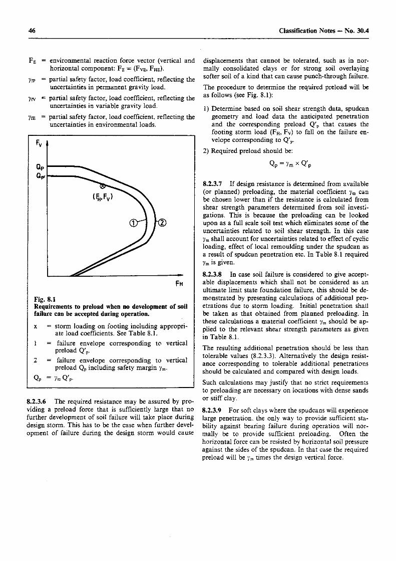
46 Classification Notes — No. 30.4
F e = environmental reaction force vector (vertical and horizontal component: FE = (FVE, FHE).
>vp = partial safety factor, load coefficient, reflecting the uncertainties in permanent gravity load.
yrv = partial safety factor, load coefficient, reflecting the uncertainties in variable gravity load.
7rE = partial safety factor, load coefficient, reflecting the uncertainties in environmental loads.
Fig. 8.1 Requirements to preload when no development of soil failure can be accepted during operation.
x = storm loading on footing including appropri-ate load coefficients. See Table 8.1.
1 = failure envelope corresponding to vertical preload Q'p.
2 = failure envelope corresponding to vertical preload Qp including safety margin ym.
Qp = /mQV
8.2.3.6 The required resistance may be assured by pro-viding a preload force that is sufficiently large that no further development of soil failure will take place during design storm. This has to be the case when further devel-opment of failure during the design storm would cause
displacements that cannot be tolerated, such as in nor-mally consolidated clays or for strong soil overlaying softer soil of a kind that can cause punch-through failure.
The procedure to determine the required preload will be as follows (see Fig. 8.1):
1) Determine based on soil shear strength data, spudcan geometry and load data the anticipated penetration and the corresponding preload Q'p that causes the footing storm load (FH, Fv) to fall on the failure en-velope corresponding to Q'p.
2) Required preload should be:
Qp = 7m x Q , p
8.2.3.7 If design resistance is determined from available (or planned) preloading, the material coefficient ym can be chosen lower than if the resistance is calculated from shear strength parameters determined from soil investi-gations. This is because the preloading can be looked upon as a full scale soil test which eliminates some of the uncertainties related to soil shear strength. In this case ym shall account for uncertainties related to effect of cyclic loading, effect of local remoulding under the spudcan as a result of spudcan penetration etc. In Table 8.1 required ym is given.
8.2.3.8 In case soil failure is considered to give accept-able displacements which shall not be considered as an ultimate limit state foundation failure, this should be de-monstrated by presenting calculations of additional pen-etrations due to storm loading. Initial penetration shall be taken as that obtained from planned preloading. In these calculations a material coefficient ym should be ap-plied to the relevant shear strength parameters as given in Table 8.1.
The resulting additional penetration should be less than tolerable values (8.2.3.3). Alternatively the design resist-ance corresponding to tolerable additional penetrations should be calculated and compared with design loads. Such calculations may justify that no strict requirements to preloading are necessary on locations with dense sands or stiff clay.
8.2.3.9 For soft clays where the spudcans will experience large penetration, the only way to provide sufficient sta-bility against bearing failure during operation will nor-mally be to provide sufficient preloading. Often the horizontal force can be resisted by horizontal soil pressure against the sides of the spudcan. In that case the required preload will be ym times the design vertical force.
47 Classification Notes — No. 30.4
Table 8.1 Partial safety factors for foundation stability checks. Check Load coefficients Material
coeffi-cient ;m
Check }'fp yrv ym
Material coeffi-
cient ;m
Bearing capacity check based on re-quirements to pre-loading
1.0 1.0 # 1.3/1.0 ** 1.1
Bearing capacity check based on available shear strength parameters
1.0 1.0 *
1.3/1.0 ** 1.3/1.2 ***
Sliding check 1.0 1.0 * 1.3/1.0 ** 1.3
* For bearing capacity checks, the characteristic loads should be based on maximum variable load, for sliding checks on minimum variable load. ** A load coefficient of 1.0 may be accepted when the en-vironmental loads are calculated based on a deterministic description of the associated environmental conditions in accordance with the MOU Rules Pt.3 Ch.l Sec.3 B306. *** 1.3 applies to undrained shear strength. 1.2 applies to coefficient of internal soil friction.
8.2.3.10 For the special case of a limited soft layer on top of a stiff layer, a moderate preload may bring the spudcan down to contact with the stiff layer. In this case the failure criterion may be allowable additional pene-tration, using an approach similar to that described in 8.4.8.
8.2.3.11 For the special case of stiff soil overlaying soft soil, the failure mode of punch-through failure will have to be investigated. One should first check whether punch-through failure is likely, by considering contact with full spudcan area on the stiff soil and check the punch-through condition using the shear strength data from soil investigations. In this process one should use the high value of ym from Table 8.1. If this check does not result in sufficient punch-through resistance, the punch-through resistance will have to be obtained by sufficient preload. The required preload can be obtained as de-scribed in 8.2.3.6 using the low value of ym from Table 8.1.
In this case the rig should be able to withstand the punch-through during preloading under controlled con-ditions for the punch-through penetrations in question. If not the rig should be rejected to operate at the partic-ular site. Analysis of punch-through failure is covered in 8.2.4.
8.2.3.12 Formulae that may be used for bearing capac-ity calculations for various idealized soil conditions are given in 4.4. If the soil conditions are difficult to idealize towards those dealt with in 4.4, more elaborate analysis may be required with methods that can account for more complex soil shear strength profiles.
8.2.3.13 For sliding of a leg, the limit state of failure can be defined as follows:
- ^ - ^ A - P H E
where
R h = characteristic horizontal resistance. 7m = partial safety factor related to uncertainties in de-
termination of horizontal resistance. FHE = horizontal force resulting from environmental
loading. 7fE = partial safety factor reflecting uncertainties in en-
vironmental loads.
8.2.3.14 Methods for calculating the horizontal sliding resistance are given in 8.2.5. When determining the sliding resistance as friction due to vertical forces on the spudcan, the vertical force should be taken as:
Fy = yfp FyP + yfy F v v + y^ F V E
where notations are as given in 8.2.3.5. As variable load, the lowest possible load should be used.
8.2.3.15 Requirements to partial safety factors to be used for sliding checks are given in Table 8.1. Normally it is only for foundations on sand where sliding may be critical.
8.2.3.16 If a jack-up is to be located near a depression of the seabed, as e.g. created by a previous jack-up in-stallation, the effect of such depressions on different pen-etration of legs, on stability of individual legs and on the general stability of the jack-up should be considered. The resulting leg deflections of one footing slide into an ex-isting footprint depression, may cause damage to the jack-up.
8.2.3.17 The possibility for scour cf the soil around the foundations should be evaluated. Scour can lead to. un-expected footing penetrations. A programme for in-spection of scour should be available, and criteria should be given for remedial actions if necessary. When sand is overlaying soft clay, penetration of the spudcan due to scour may turn the foundation from being safe to being unsafe against punch-through failure. In such conditions scour protection should be provided.
8.2.3.18 Scour protection may include:
• Gravel dumping prior to or after installation • Installation of artificial seaweed • Installation of gravel bags or grout mattresses after
jack-up installation • Penetration to scour-safe depth by jetting/airlifting for
rigs which are provided with adequate equipment.
8.2.4 Analysis of punch-through failure
8.2.4.1 Analysis of punch-through failure can be per-formed by assuming that the vertical pressure from the foundation area distributes into a wider area as illustrated on Fig. 8.2.
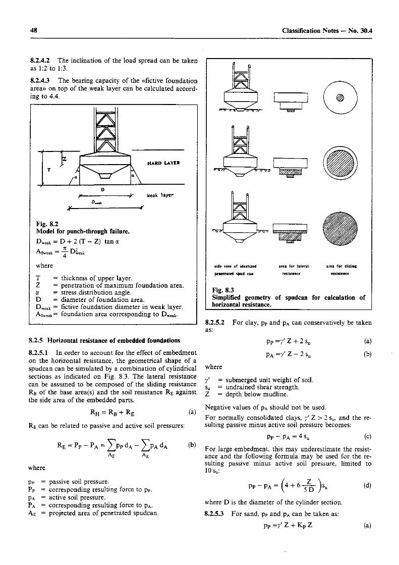
48 Classification Notes — No. 30.4
8.2.4.2 The inclination of the load spread can be taken as 1:2 to 1:3.
8.2.4.3 The bearing capacity of the «fictive foundation area» on top of the weak layer can be calculated accord-ing to 4.4.
Fig. 8.2 Model for punch-through failure. Dweak = D + 2 (T — Z) tan a
Aoweak ~ Dweak
where T = thickness of upper layer. Z = penetration of maximum foundation area. a = stress distribution angle. D = diameter of foundation area. DWeak = Active foundation diameter in weak layer. Aoweak̂ foundation area corresponding to DWeak-
8.2.5 Horizontal resistance of embedded foundations
8.2.5.1 In order to account for the effect of embedment on the horizontal resistance, the geometrical shape of a spudcan can be simulated by a combination of cylindrical sections as indicated on Fig. 8.3. The lateral resistance can be assumed to be composed of the sliding resistance RB of the base area(s) and the soil resistance RE against the side area of the embedded parts.
Rh = Rb + Re (a) R e can be related to passive and active soil pressures:
R E = P P - P A = ] T p P d A - Y f A d A
where
Pp = passive soil pressure. PP = corresponding resulting force to pP. pA = active soil pressure. PA = corresponding resulting force to pA. Ae = projected area of penetrated spudcan.
(b)
T7TVH?
side view of idealized
penetrated spud can
area for lateral
resistance
area for sliding resistance
Fig. 8.3 Simplified geometry of spudcan for calculation of horizontal resistance.
8.2.5.2 For clay, pP and pA can conservatively be taken as:
pP = / Z + 2 su
pA = / Z - 2 su
(a)
(b)
where
y' = submerged unit weight of soil. su = undrained shear strength. Z = depth below mudline.
Negative values of pA should not be used. For normally consolidated clays, / Z > 2 su, and the re-sulting passive minus active soil pressure becomes:
Pp ~ PA = 4 su (c)
For large embedment, this may underestimate the resist-ance and the following formula may be used for the re-sulting passive minus active soil pressure, limited to 10 su:
where D is the diameter of the cylinder section.
8.2.5.3 For sand, pp and pA can be taken as:
pP = / Z + KP Z
(d)
(a)
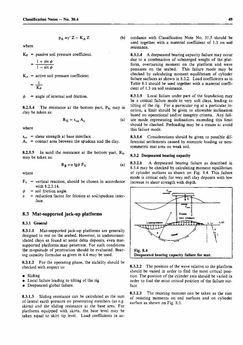
49 Classification Notes — No. 30.4
P A = V ' Z - K A Z (b)
where
Kp = passive soil pressure coefficient.
_ 1 + sin (j> 1 — sin 0
K a = active soil pressure coefficient. = J _
KP
(j> = angle of internal soil friction.
8.2.5.4 The resistance at the bottom part, PB, may in clay be taken as:
r H = suo Ao (a)
where
suo = shear strength at base interface. A0 = contact area between the spudcan and the clay.
8.2.5.5 In sand the resistance at the bottom1 part, RB, may be taken as:
R b =a tg(j> F v (a)
where
Fv = vertical reaction, should be chosen in accordance with 8.2.3.14.
<t> = soil friction angle. a = reduction factor for friction at soil/spudcan inter-
face.
8.3 Mat-supported jack-up platforms
8.3.1 General
8.3.1.1 Mat-supported jack-up platforms are generally designed to rest on the seabed. However, in underconsol-idated clays as found at some delta deposits, even mat-supported platforms may penetrate. For such conditions the magnitude of penetration should be evaluated. Bear-ing capacity formulae as given in 4.4 may be used.
8.3.1.2 For the operating phase, the stability should be checked with respect to:
• Sliding • Local failure leading to tilting of the rig • Deepseated global failure.
8.3.1.3 Sliding resistance can be calculated as the sum of lateral earth pressure on penetrating members (as e.g. skirts) and the sliding resistance at the base area. For platforms equipped with skirts, the base level may be taken equal to skirt tip level. Load coefficients in ac-
cordance with Classification Note No. 31.5 should be used together with a material coefficient of 1.3 on soil resistance.
8.3.1.4 A deepseated bearing capacity failure may occur due to a combination of submerged weight of the plat-form, overturning moment on the platform and wave pressures on the seabed. This failure mode may be checked by calculating moment equilibrium of cylinder failure surfaces as shown in 8.3.2. Load coefficients as in Table 8.1 should be used together with a material coeffi-cient of 1.3 on soil resistance.
8.3.1.5 Local failure under part of the foundation may be a critical failure mode in very soft clays, leading to tilting of the rig. For a particular rig at a particular lo-cation, a limit should be given to allowable inclination based on operational and/or integrity criteria. Any fail-ure mode representing inclinations exceeding this limit should be checked. Preloading may be a means to avoid this failure mode.
8.3.1.6 Considerations should be given to possible dif-ferential settlements caused by eccentric loading or non-symmetric mat area on weak soil.
8.3.2 Deepseated bearing capacity
8.3.2.1 A deepseated bearing failure as described in 8.5.4 may be checked by calculating moment equilibrium of cylinder surfaces as shown on Fig. 8.4. This failure mode is critical only for very soft clay deposits with low increase in shear strength with depth.
8.3.2.2 The position of the wave relative to the platform should be varied in order to find the most critical posi-tion. The position of the cylinder axis should be varied in order to find the most critical position of the failure sur-face.
8.3.2.3 The resisting moment can be taken as the sum of resisting moments on end surfaces and on cylinder surface as shown on Fig. 8.5.
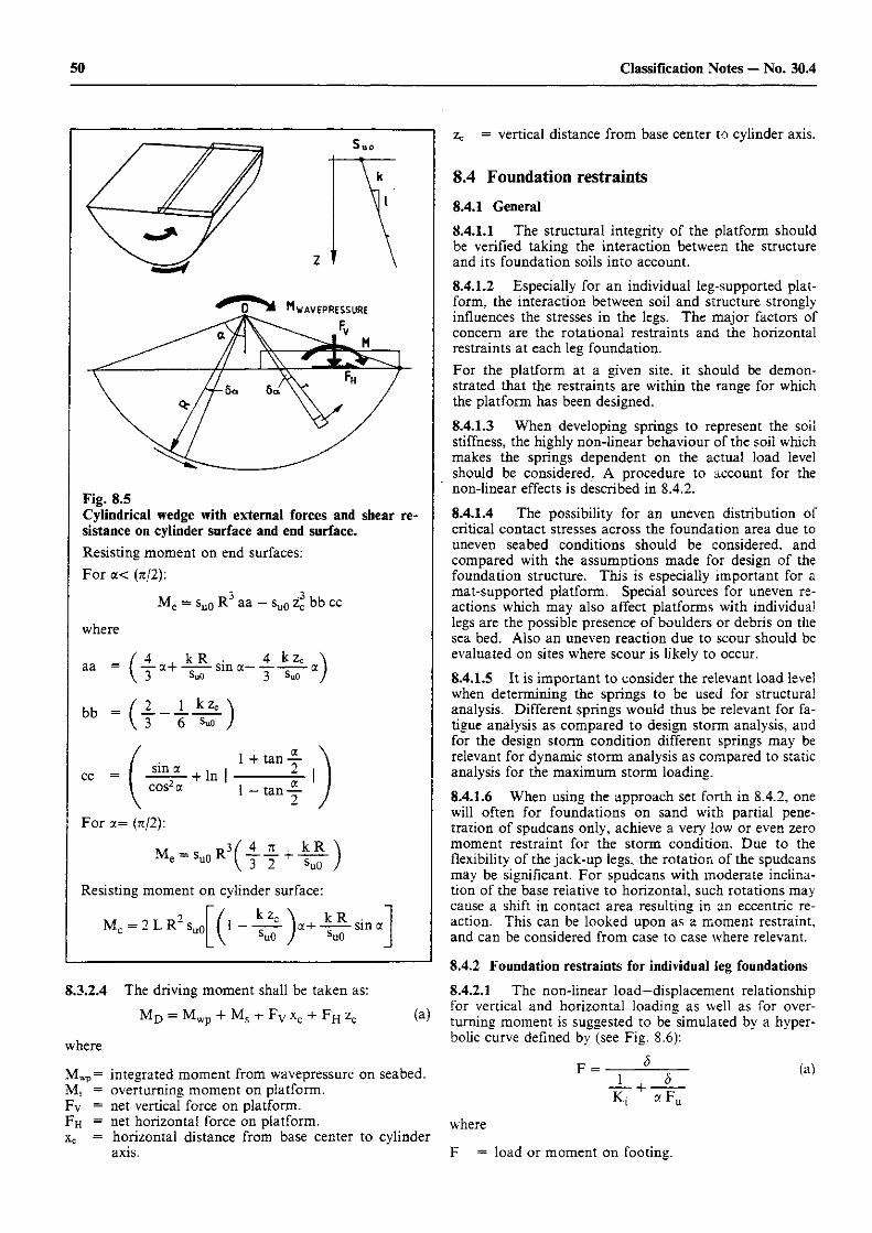
50 Classification Notes — No. 30.4
Fig. 8.5 Cylindrical wedge with external forces and shear re-sistance on cylinder surface and end surface. Resisting moment on end surfaces: For a< (n/2):
3 3 Me = su0 R a a - su0 zc bb cc
where
aa £ a + _kR_ s i n 4_ _kzL a> 3 suo 3 su0 j
bb =
cc =
- ( = ( 2 1 k 2 c \
V 3 6 suo )
sm a cos2 a
+ In 1 + tan 2_ l - t a n - 2 -
For a= (71/2):
\A c 1>3/ 4 7T . k R \
Resisting moment on cylinder surface:
Mc = 2 L R a + 4 - ^ s i n a su0
8.3.2.4 The driving moment shall be taken as: M D = M W P + M S + F V xc -f F H ZC (a)
where
zc = vertical distance from base center to cylinder axis.
8.4 Foundation restraints 8.4.1 General 8.4.1.1 The structural integrity of the platform should be verified taking the interaction between the structure and its foundation soils into account. 8.4.1.2 Especially for an individual leg-supported plat-form, the interaction between soil and structure strongly influences the stresses in the legs. The major factors of concern are the rotational restraints and the horizontal restraints at each leg foundation. For the platform at a given site, it should be demon-strated that the restraints are within the range for which the platform has been designed.
8.4.1.3 When developing springs to represent the soil stiffness, the highly non-linear behaviour of the soil which makes the springs dependent on the actual load level should be considered. A procedure to account for the non-linear effects is described in 8.4.2.
8.4.1.4 The possibility for an uneven distribution of critical contact stresses across the foundation area due to uneven seabed conditions should be considered, and compared with the assumptions made for design of the foundation structure. This is especially important for a mat-supported platform. Special sources for uneven re-actions which may also affect platforms with individual legs are the possible presence of boulders or debris on the sea bed. Also an uneven reaction due to scour should be evaluated on sites where scour is likely to occur.
8.4.1.5 It is important to consider the relevant load level when determining the springs to be used for structural analysis. Different springs would thus be relevant for fa-tigue analysis as compared to design storm analysis, and for the design storm condition different springs may be relevant for dynamic storm analysis as compared to static analysis for the maximum storm loading. 8.4.1.6 When using the approach set forth in 8.4.2, one will often for foundations on sand with partial pene-tration of spudcans only, achieve a very low or even zero moment restraint for the storm condition. Due to the flexibility of the jack-up legs, the rotation of the spudcans may be significant. For spudcans with moderate inclina-tion of the base relative to horizontal, such rotations may cause a shift in contact area resulting in an eccentric re-action. This can be looked upon as a moment restraint, and can be considered from case to case where relevant.
8.4.2 Foundation restraints for individual leg foundations 8.4.2.1 The non-linear load—displacement relationship for vertical and horizontal loading as well as for over-turning moment is suggested to be simulated by a hyper-bolic curve defined by (see Fig. 8.6):
Mwp= integrated moment from wavepressure on seabed. Ms = overturning moment on platform. Fv = net vertical force on platform. Fh = net horizontal force on platform. xc = horizontal distance from base center to cylinder
axis.
F = (a)
K{ + a F„
where
F = load or moment on footing.
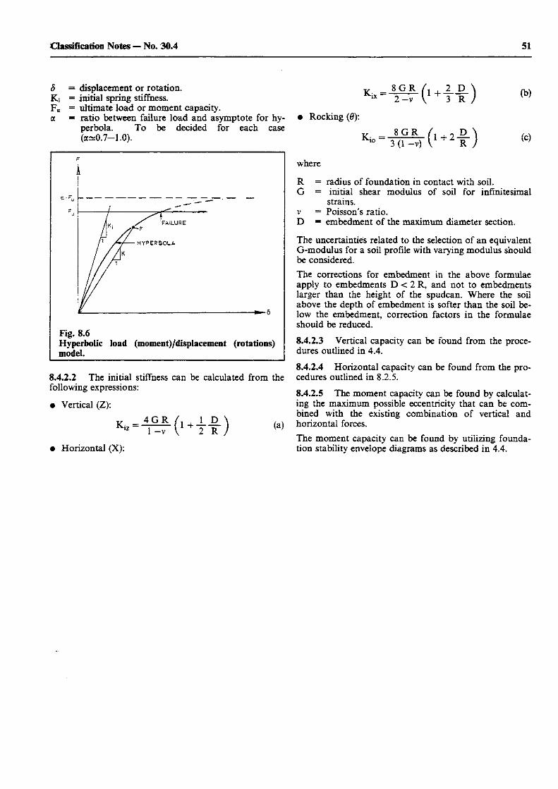
51 Classification Notes — No. 30.4
8 = displacement or rotation. Kj = initial spring stiffness. Fu = ultimate load or moment capacity, a = ratio between failure load and asymptote for hy-
perbola. To be decided for each case (a~0.7-1.0).
r
A
Fig. 8.6 Hyperbolic load (moment)/displacement (rotations) model.
8.4.2.2 The initial stiffness can be calculated from the following expressions:
• Vertical (Z):
^ 4 G R / , 1 D \ , v
• Horizontal (X):
v 8 G R /1 , 2 D \
• Rocking (0):
where
R = radius of foundation in contact with soil. G = initial shear modulus of soil for infinitesimal
strains, v = Poisson's ratio. D = embedment of the maximum diameter section. The uncertainties related to the selection of an equivalent G-modulus for a soil profile with varying modulus should be considered. The corrections for embedment in the above formulae apply to embedments D < 2 R, and not to embedments larger than the height of the spudcan. Where the soil above the depth of embedment is softer than the soil be-low the embedment, correction factors in the formulae should be reduced.
8.4.2.3 Vertical capacity can be found from the proce-dures outlined in 4.4.
8.4.2.4 Horizontal capacity can be found from the pro-cedures outlined in 8.2.5.
8.4.2.5 The moment capacity can be found by calculat-ing the maximum possible eccentricity that can be com-bined with the existing combination of vertical and horizontal forces. The moment capacity can be found by utilizing founda-tion stability envelope diagrams as described in 4.4.
52 Classification Notes — No. 30.4
9. References 11/ Dennis N.D. and Olson R.E. (1983):
«Axial Capacity of Steel Pipe Pipes in Clay», Proc. of the Conference on Geotechnical Practice in Offshore Engineering, Austin, Texas, April.
12/ Kirby R.C., Esrig M.I. and Murphy B.S. (1983): «General Effective Stress Method for Piles in Clay, Part I — Theory», Proc. of the Conference on Geotechnical Practice in Offshore Engineering, Austin, Texas, April.
/3/ Randolph M.F. (1983): «Design Considerations for Offshore Piles», Proc. of the Conference on Geotechnical Practice in Offshore Engineering, Austin, Texas, April.
/4/ Semple R.M. and Rigden W.J. (1984): «Shaft Capacity of Driven Pipe Piles in Clay», Symposium on Analysis and Design of Piled Founda-tions in conjunction with ASCE National Convention, San Francisco.
15/ Kraft L.M., Cox W.R. and Verner E.A. (1981): «Pile Load Tests: Cyclic Loads and Varying Load Rates», Journal of the Geotechnical Division, ASCE, Vol. 107, No.GTl, January.
/6/ Karlsrud K., Nadim F. and Haugen T. (1986): «Piles in Clay under Cyclic Loading)), Proc. of the 3rd International Conference on Numer-ical Methods in Offshore Piling, Nantes.
/7/ Ove Arup and Partners (1986): «Comparison of British and Norwegian Research on the Behaviour of Piles and Anchors for Buoyant Structures)), Offshore Technology Report No. OTH 86218, De-partment of Energy, London.
/8/ American Petroleum Institute, Recommended Practice for Planning, Designing and Constructing Fixed Off-shore Platforms (1987), API RP 2A, April, 17th Edi-tion.
19! Burland J.F. (1973): «Shaft Friction of Piles in Clay — A Simple Funda-mental Approach)), Ground Engineer, Vol.6, No.3.
/10/ Vijayvergiya V.N. and Focht J.A. (1972): «A New Way to Predict the Capacity of Piles in Clay)), Proc. of the Offshore Technology Conference, Vol.2, pp.865—874, Houston.
/II/ Kraft L.M., Focht J.A. and Amerasinghe S.F (1981): «Friction Capacity of Piles Driven into Clay)), Journal of the Geotechnical Division, ASCE, Vol.107, GT11, November.
/12/ Janbu N. (1976): «Static Bearing Capacity of Friction Piles», Geotechnical Division of Norwegian Institute of Technology, Bulletin No.9, Trondheim.
/13/ Flaate K. and Seines P. (1977): «Side Friction of Piles in Clay)), Proc. of the 9th International Conference on Soil Me-chanics and Foundation Engineering, Tokyo.
/14/ American Petroleum Institute, Recommended Prac-tice for Planning, Designing and Constructing Fixed Offshore Platforms (1982), API RP 2A, January, 13th Edition.
/15/ Dennis N.D. and Olson R.E. (1983): «Axial Capacity of Steel Pipe Pipes in Sand)), Proc. of the Conference on Geotechnical Practice in Offshore Engineering, Austin, Texas, April.
/16/ Toolan F.E and Fox D.A. (1977): «Geotechnical Planning of Piled Foundations for Off-shore Platforms)). Institution of Civil Engineers, Proceedings, Part I, Vol.62, May.
/ II / Ruiter J. de and Beringen F.L. (1979): «Pile Foundations for Large North Sea Structures)), Marine Technology, Vol.3, No.3.
/18/ Proc. of the International Conference on Calcareous Sediments (1988), Engineering for Calcareous Sedi-ments, Perth 15—18 March, Volumes 1 and 2.
/19/ Poulos H. (1983): «Cyclic Axial Pile Response — Alternative Analysis)), Proc. of the Conference on Geotechnical Practice in Offshore Engineering, Austin, Texas. April.
120/ Matlock H. (1970): Correlations for Design of Laterally Loaded Piles in Soft Clay)), Proc. of the Offshore Technology Conference, Paper No. OTC 1204, Houston.
/2l/ Reese L.C., Cox W.R. and Koop F.D. (1974): «Analysis of Laterally Loaded Piles in Sand)>, Proc. of the 6th Offshore Technology Conference, Pa-per No. OTC 2080, Houston.
/22/ O'Neill M.W. and Murchinson J.M. (1983): «An Evaluation of p—y Relationships in Sands)), A report to the American Petroleum Institute, May.
/23/ Focht J.A. and Koch J.J. (1973): «Rational Analysis of the Lateral Performance of Offshore Pile Groups)), Proc. of the Offshore Technology Conference, Vol.2, Paper No. 1896, Houston.
/24/ Poulos H.G. and Davis E.H. (1980): «Pile Foundation Analysis and Design)), John Wiley and Sons.
/25/ Det norske Veritas: «Rules for Classification of Fixed Offshore Installations)), Part 3 Structures; Chapter 1 Structural Design, Gen-eral; Section 9 Foundation Design.
/25A/ Eide O. and Andersen K.H. (1984): «Foundation Engineering for Gravity Structures in the Northern Sea)), International Conference on Case Histories in Geo-technical Engineering, St. Louis, USA. May. Also published in NGI publication no. 154.
126/ Andersen K.H. (1976): «Behaviour of Clay Subjected to Undrained Cyclic Loading)), Proc. of the International Conference on the Behavi-our of Offshore Structures (BOSS'76), Vol.1, pp.392—403, Trondheim.
53 Classification Notes — No. 30.4
/27/ Foss I. and Dahlberg R. (1979): «FIP State of Art Report: Foundations of Concrete Gravity Structures in the North Sea», Chapter 3: Foundation Design Methods for Gravity Structures, pp.33—55.
/28/ Andersen K.H. and Lauritzen R. (1988): «Bearing Capacity for Foundations with Cyclic Loads», Journal of Geotechnical Engineering, Vol.114, No. 5, May.
/29/ Janbu N. (1985): «Soil Models in Offshore Engineering)), The 25th Ranking Lecture, Geotechnique, Vol.35, No.3, September.
/30/ Janbu N., Grande L.O. and Eggereide K. (1976): «Effective Stress Stability Analysis for Gravity Structures)), Proc. of Behaviour of Offshore Structures Conference, Trondheim, Vol.1, pp.449—466.
/31/ Tokheim O. (1976): «A model for soil behaviour)), Dr.techn. thesis, Geotechnical Division, Norwegian Institute of Technology.
/32/ Morgenstern N.R. and Price V.E. (1965): «The Analysis of the Stability of General Slip Surfaces)), Geotechnique, Vol. 15, No. 1.
/33/ Janbu N. (1973): «Slope Stability Computations, Embankment-dam Engineering)), Casagrande volume (Ed. R.C. Hirschfeld and S.J. Poulos), John Wiley and Sons Inc., pp.47—86, New York.
/34/ Lauritzen R and Schjetne K. (1976): «Stability Calculations for Offshore Gravity Structures)), Offshore Technology Conference, Paper No. OTC 2431, Houston.
/35/ Clausen C.J.F. (1985): «Bearing 1, a Computer Program for Analysis of the Bearing Capacity of a Foundation on Clay Subjected to Undrained Loading)), Virum, Denmark.
736/ Brinch-Hansen J. (1970): «A Revised and Extended Formula for Bearing Capacity)), Geoteknisk Institut, Bulletin No.28, p.5—11, Copen-hagen.
/37/ Caquot A. and Kerisel J. (1953): «Sur la Terme de Surface dans le Calcul des Fonda-tions en Milieu Pulverult», Proc. of the 3rd International Conference on Soil Me-chanics and Foundation Engineering, Vol.1, Zurich.
/38/ Davis E.H. and Booker J.R. (1973): «The Effect of Increasing Strength with Depth on the Bearing Capacity of Clays)), Geotechnique, Vol.23, No.4.
/39/ Salencon J. and Matar M. (1983): «Bearing Capacity of Circular Shallow Foundations in Foundation Engineering)),
Soil Properties, Foundation Design and Construction, Vol.1, pp.159—168, Presses de 1'Ecole et Nationale des Ponts et Chausees.
/40/ Janbu N. (1963): «Soil Compressibility as Determined by Oedometer and Triaxial Tests)), Proc. of the 3rd European Conference on Soil Me-chanics, Wiesbaden, Vol.1.
/41/ Janbu N. (1967): «Settlement Calculations Based on the Tangent Mo-dulus Concept)), Three guest lectures at Moscow State University, Bul-letin No.2, Soil Mechanics, Norwegian Institute of Technology, Trondheim.
/42/ Dahlberg R. (1975): «Settlement Characteristics of Preconsolidated Natural Sands)), Ph.D. thesis, Soil and Rock Mechanics, Royal Insti-tute of Technology, Document No. Dl:1975, Stock-holm.
/43/ Boussinesq J. (1885): «Application des Potensials a l'Etude de l'Equilibre et du Mouvement des Solids Elastiques)), Gauthier-Villiers, Paris.
/44/ Timoschenko S. and Goodier J.N. (1951): «Theory of Elasticity)), McGraw-Hill Book Company, 2nd Edition, New York.
/45/ Frohlich D.K. (1934): «Druckverteiligung im Baugrunde, mit besonderer Beriicksichtigung der Plastischen Erscheinungen)), Springer, Berlin.
/46/ Jaky J. (1944): «The Coefficient of Earth Pressure at Rest)), J. Soc., Hungarian Architects and Engineers, Buda-pest.
/47/ Buisman A.S.K. (1932): «Drukverdeeling in Bouwgrond in Verband met On-gelijke Samendrukoarheid in Horizontal en Vertikale Richting)), De Ing., Vol.47, Bouw- en Waterbouwkunde.
748/ De Beer E.E. (1970): «Grondmechanica)), Deel II, Funderingen, N.V. Standard Boekhandel, Delft.
/49/ Janbu N., Bjerrum L. and Kj<ernsli B. (1964): «Soil Mechanics Applied to some Engineering Problems)), The Norwegian Geotechnical Institute, Publication No. 16, Oslo.
150/ Brinch-Hansen J. (1966): «Simplified Stress Determination in Soils)), The Danish Geotechnical Institute, Bulletin No.20, Copenhagen.
751/ Janbu N. (1965): Consolidation of Clay Layers based on Non-Linear Stress Strain)), Proc. of the 5th International Conference on Soil Me-chanics and Foundation Engineering, Montreal.
7527 Andersen K.H. (1986):
54 Classification Notes — No. 30.4
«Calculation of Soil Spring Stiffnesses and Cyclic Dis-placements of Offshore Gravity Platforms)), Seminar on «Plattformer til havs — samvirke mellom jord og konstruksjon», NTH, January.
/53/ Gazetas G. (1983): «Analysis of Machine Foundation Vibrations: State of the Art», Soil Dynamics and Earthquake Engineering, Vol. 2, No. 1.
/54/ Whitman R.V. (1976): «Soil—Platform Interaction)), Proc. of the International Conference on the Behavi-our of Offshore Structures (BOSS 76).
155/ Wong H.L. and Luco J.E. (1985): «Tables of Impedance Functions for Square Founda-tions on Layered Media», Soil Dynamics and Earthquake Engineering, Vol. 4, No. 2.
156/ Waas G. and Werkle H. (1984): «Schwingungen von Fundamenten auf inhomogenen Baugrund», VDI Berichte 536.
/57/ Gazetas G. (1991): «Formulas and Charts for Impedance of Surface and Embedded Foundations)), ASCE Journal of Geotechnical Engineering, Vol. 117, No. 9, September.
/58/ Randolph M.F. and Wroth C.P. (1978): «Analysis of Deformation of Vertically Loaded Piles)), ASCE Journal of Geotechnical Engineering, Vol. 104, No. GT12, December.
/59/ Kraft L.M., Ray R.P. and Kagawa T.: (1981): «Theoretical t-z curves)), ASCE Journal of Geotechnical Engineering, Vol. 107, No. GT11, November.
/60/ Poulos H.G. and Davis E.H. (1974): «Elastic Solutions for Soil and Rock Mechanics)), J. Wiley & Sons Inc.
/61/ Lacasse S and D'Orazio T.B. (1988): «Soil Reaction Stresses on Offshore Gravity Platforms)), ASCE Journal of Geotechnical Engineering, Vol. 114, No. 11, November.
Related Documents