DNA Segmentation Through the Bayesian Approach

JOURNAL OF COMPUTATIONAL BIOLOGYVolume 7, Numbers 1/2, 2000Mary Ann Liebert, Inc.Pp. 215–231

DNA Segmentation Through the Bayesian Approach

V.E. RAMENSKY,1 V.JU. MAKEEV,1 M.A. ROYTBERG,2 and V.G. TUMANYAN1

ABSTRACT

We present a new approach to DNA segmentation into compositionally homogeneous blocks.The Bayesian estimator, which is applicable for both short and long segments, is used toobtain the measure of homogeneity. An exact optimal segmentation is found via the dynamicprogramming technique. After completion of the segmentation procedure, the sequence com-position on different scales can be analyzed with � ltration of boundaries via the partitionfunction approach.

Key words: nucleic acids, nucleotide composition, Bayesian statistics, segmentation.

1. INTRODUCTION: COMPOSITIONAL SEGMENTATION OFBIOLOGICAL SEQUENCES

Nucleotide sequences typically display correlations in nucleotide compositions, which are foundboth on small scales (Fickett, 1982; Frank and Makeev, 1997; Kypr and Mrazek, 1986; Mrazek and

Kypr, 1994; Trifonov and Sussman, 1980; see also the literature on Markov chains, e.g., Guigo andFickett, 1995) and on large scales (Sueoka, 1959; Bains, 1993; Bernardi, 1989; Bernardi, 1995; Bernardiet al., 1985; Chechetkin and Lobzin, 1998; D’Onofrio et al., 1991; Karlin and Brendel, 1993; Kypr andMrazek, 1995; Kypr et al., 1989; Li, 1994; Li, 1997; Ossadnik et al., 1994; Peng et al., 1992; Trifonov andSussman, 1980; Tsonis et al., 1991). Several biological issues are believed to be related to these correlations.Among other examples, one can mention the presumption of Bernardi et al. that many genomes of highereukaryotes contain long regions of quasi-uniform composition, the isochores (Bernardi, 1989; Bernardi,1995; D’Onofrio et al., 1991), the compositional difference between exons and introns (Guigo and Fickett,1995; Herzel and Grosse, 1997), simple repeats (e.g., Li and Kaneko, 1992), tracts in splicing sites (Gelfand,1992; Gelfand, 1995), and DNA sites of factor binding (Gelfand and Koonin, 1997).

The local nucleotide composition is taken into account in many algorithms developed for the search ofdifferent patterns in DNA sequences (Krogh et al., 1994(a); Krogh et al., 1994(b); Reese et al., 1997).Algorithms of this kind usually employ a � xed window, the length of which can affect the results. Thepreliminary compositional segmentation, which breaks a DNA sequence into homogeneous subsequences(blocks or segments), can therefore improve the perfomance of the pattern search.

Recently Bernaola-Galvan et. al. (1996) (see also Roman-Roldan et al. (1998)) have put forward asegmentation algorithm, where they used an approach based on the Jensen-Shannon divergence measureemployed in various image-processing applications.The sequence is divided into two adjacent subsequencesif the compositionsof the resulting segments differ at the given level of statistical con� dence. This procedureis repeated for each of the two resulting subsequences until the whole sequence becomes segmented

1Engelhardt Institute of Molecular Biology, Vavilova, 32 Moscow, 117984 Russia.2Institute of Mathematical Problems of Biology, Institutskaya, 4 Puschino, Moscow region 142292 Russia.

215

216 RAMENSKY ET AL.

into domains differing from each other in their composition. The segments so de� ned are neighborhood-dependent.

This technique, although conceptually simple and computationally ef� cient, has two basic disadvantages.First, regardless of the divergence measure chosen, the hierarchical segmentation procedure does not ensurethat the true optimal segmentation will be attained. Indeed, the � rst boundary, which divides the sequenceinto two subsequences, and actually re� ects the compositions averaged over very large distance, is retainedfor the whole subsequent procedure, even if it fails to be appropriate at the later stages of the segmentationprocess when it separates smaller blocks.

Second, this procedure requires a criterion for termination of cutting. To this end, Bernaola-Galvan et al.(1996) use statistical inference. The segmentation thus becomes dependent on the given threshold valueindicating that the compositions of subsequences are signi� cantly different. With the point estimator ofthe frequency of each letter used by Bernaola-Galvan et al. (1996), it is necessary that the segments arelong enough to secure reliable statistics. This critical block length depends on the composition of thesegments. This additional requirements may create dif� culties in comparing the resulting segmentationwith the functional structure of the sequence.

We believe that the optimal segmentation algorithm should be free of both shortcomings, with all possiblecon� gurations of boundaries taken into account and the short segments considered on an equal basis withthe long ones.

Moreover, the very de� nition of homogeneous segments depends on the scoring system. Even such asimple sequence as AAAACACACCCC brings about the question of what segmentation, “AAAA-CACA-CCCC ”or “AAAACA-CACCCC ,” is better. Different scoring systems can yield different answers.

Finally, the necessity to test all possible boundary con� gurations is a serious computational problem,since the number of possible segmentations is exponentially large (if a boundary is to be set between anytwo neighboring letters, this quantity equals 2N ¡ 1, where N is the sequence length). The computationaltime may be reduced with scores of a special type, for which dynamic programming or another similartechnique may be employed.

In the context described, the Bayesian approach turns out to be highly expedient. For the problemdiscussed, it is intuitively very clear. All the integrals involved in constructing the Bayesian estimatorscan be taken analytically, which is a rare case in the practical application of the Bayesian statistics. TheBayesian estimator does not degenerate for short blocks, and one can easily incorporate it into the dynamicprogramming scheme.

In the framework of general Bayesian inference, this problem relates to the multiple-changepoint iden-ti� cation (Chernoff and Zacks, 1964; Smith, 1975; Booth and Smith, 1982). The general theory, withexamples, is presented by Stephens (1994). Segmentations of sequences with the Bayesian approach wasrecently discussed by Liu and Lawrence (1999) (see also Lawrence (1997)). Their paper can also serve asan excellent introduction to the Bayesian approach in bioinformatics. Basically, their technique is free ofthe disadvantages of the approach of Ramon-Roldan et al. and begins with segmentation of the sequenceinto a � xed number of blocks, with subsequent calculation of the boundary probability distribution usinga sampling procedure (see also Stephens (1994)). We discuss the differences of this algorithm with oursin detail in Section 6. The only remark to be made in advance is that we use sets of possible boundariesrather than probability distributions for borders and do not use sampling.

Our algorithm consists of the following two stages: (i) given the sequence, the possible con� gurations ofboundaries between blocks, i.e., the segmentations, are tested. For each segmentation a likelihood functionis calculated. This function is maximized over all possible segmentations via dynamic programming,yielding the optimal segmentation. As a rule, the optimal segments are relatively short. Therefore, toobtain segmentation with larger segment lengths, some neighboring blocks of similar composition shouldbe merged, that is, some boundaries should be � ltered out.

For � ltration (ii), we calculate the probability of every optimal boundary. To this end, we use the partitionfunction of the whole sequence, as well as the partition functions of the subsequences to the right and tothe left of the boundary under evaluation. After � ltration, only boundaries with probabilities higher than agiven threshold are retained, providing the (suboptimal) segmentation with longer segments.

In this paper we also discuss the practical aspects, such as the choice of the prior, the ef� cient algo-rithm, the examples of segmentation of biological sequences, and the possible future applications of themethod.

SEGMENTATION OF DNA SEQUENCES 217

2. BAYESIAN SEGMENTATION. GENERAL CONCEPT ANDCONSTRUCTION OF ESTIMATORS

2.1. The problem

Consider a symbolic sequence written in an alphabet « containing L letters. We are going to approximatethis sequence with a probabilistic model. The sequence is considered as a series of statistically independentand compositionally homogeneous blocks of arbitrary length. These blocks are of multinomial randomnature. For each block, we shall refer to the observed numbers of each letter in it as to the countsn 5 (n1, . . . nL ). These counts serve as arguments of a score function that re� ects the homogeneity ofeach block. We de� ne a segmentation as a set of boundaries separating these blocks and use block countsto estimate their compositions. Since the blocks are assumed to be statistically independent, the score forthe entire segmented sequence is a product of the scores for individual blocks.

With the score function at hand, the sequence is studied with two complementary techniques, whosecombination yields reliable results. The result of applying the � rst technique is a single optimal segmen-tation with the maximal score; the second technique consists in calculating the probabilities of boundarieswith the help of the partition function of all possible segmentations.

2.2. Optimal segmentation

To obtain the optimal segmentation, we employ a dynamic programming algorithm (Finkelstein andRoytberg, 1993), which computes it for the time proportional to the squared sequence length (see Section4). However, several various partitions often yield the same score (e.g., AACAC and A-ACAC for the marginallikelihood score; see Section 2.7) and our algorithm provides only one solution out of the many havingidentical scores.

Moreover, some of the boundaries forming the optimal segmentation are very sensitive to minor changesin the sequence. Although the scores of the optimal segmentation of the changed sequences are close tothe score of the unperturbed one, the segmentation patterns can be rather different.

The second technique can take into account the suboptimal solutions.

Boundary probabilities. Partition function. Determine the partition function of the set of segmentationsof a sequence of length N in a standard way (Finkelstein and Roytberg, 1993) by summing the probabilitiesof all possible partitions:

Z (N ) 5X

q1

X

qN ¡ 1

¦ (q1, . . . qN ¡ 1) (1)

where the indicator qk equals 1 if there is a boundary located after the letter k in the sequence, and 0otherwise; the overall q 5 (q1, . . . , qN ) determines a segmentation which has the probability ¦ (q). Thepartition function can be easily computed via the dynamic programming algorithm (see 4.2 below).

To calculate the probability of the boundary located after the letter k, one needs two partition functionsof subsequences to the left and to the right of this border, Z L and Z R respectively:

¦ (qk 5 1) 5Z L (k)Z R (N ¡ k)

Z (N ). (2)

Boundaries with higher probabilities separate blocks with higher compositional divergence. Therefore,such boundaries tend to be more stable with the sequence undergoing minor changes. The partition functionapproach cannot provide an optimal segmentation of the sequence, but can indicate which boundariesare more statistically signi� cant. Thus, the two techniques complement each other in obtaining a stablesuboptimal segmentation pattern.

In the following sections we obtain the score that re� ects the block homogeneity.

218 RAMENSKY ET AL.

2.3. Blocks of random composition. Probabilistic approach

Denote the set of letter probabilities of a multinomial (Bernoulli) sequence as s 5 fh1, h2, . . . , hL g,which is subject to the normalization condition

LX

k 5 1

hk 5 1. (3)

We shall use s to represent the composition of the block. The objective is to � nd compositions whichprovide a high probability of obtaining the block sequence in a series of random tests.

Given the composition, the probability of the counts is P (njs) 5 N !QL

i 5 1[hn ii =ni !], whereas the likeli-

hood of the individual sequence to occur is

P (S js) 5LY

i 5 1

hni . (4)

Adoption of the simplest frequency-count estimator of the composition hi 5 ni =N results in the trivialsegmentation down to the individual letters which have 100% probability; this is certainly not what weneed. Moreover, the trivial segmentation is statistically unreliable. Thus, the size of the sample should betaken into consideration, especially for very small samples. This is exactly the case for which the Bayesiantechniques excel. The Bayes estimator can be viewed as a way to directly account for the “missinginformation” when the information at hand consists of a � nite data set rather than a full distribution p(s)(Wolpert and Wolf, 1995).

2.4. Composition probability density function

The Bayesian statistics regards all the parameters of the problem as random variables. In the beginning ofthe procedure, these variables have some prior probability distribution,which can be chosen quite arbitrarily.The experimental data allow one to estimate these probability distributions via the Bayes formula. Theresult of the Bayesian estimation is again some probability distribution of the estimated quantity, ratherthan a single value considered in the classical statistics (Rozanov, 1985).

However, Bayesian and classical statistics agree for the large samples. More precisely, if we estimateparameters from large samples, the Bayesian probability distributions converge with probability 1 to thecorrect parameter values for any prior (Rozanov, 1985). Thus, the Bayesian estimators are consistent.However, the choice of prior is much more important for the small quantities of data, which is exactly ourcase, since we also consider very short blocks.

The results of previous estimations may be used as the prior for the next step. This technique is referredto as recurrent estimation and is employed, for instance, in adaptive learning algorithms.

For the composition s 5 fh1, h2, . . . , hL g, write the probability density function p(s), which is a functionde� ned on the simplex ª 5 fs : hk ¶ 0;

PLk 5 1 hk 5 1g satisfying the normalization condition:Z

ªdsp(s) 5 1. (5)

The integral above may be understood in two senses. Wolpert and Wolf regard it as an ordinaryL -dimensional integral over the region extending in each dimension from 0 to 1, whereas the func-tion under integration has support only on the simplex ª. The other point of view assumes it to be a� rst-type surface integral taken over the surface of the simplex. These two cases are different for the

pL !

multiplier related to the total surface of the simplex ª , which isp

L !(L ¡ 1)! (see normalization (3)). In our case,

this multiplier cancels in � nal equations, which thus do not depend on the form of the integral. Furtherthan that, we shall not use this multiplier.

Given some prior distribution p(s), consider a putative segment with sequence S . The Bayes theorembrings about the posterior probability density function p(sjS )

p(sjS ) 5P (S js)p(s)

P (S )(6)


where

P (S) 5

ZdsP (S js)p(s) (7)

is the normalization constant called the marginal likelihood (Stephens, 1994; Liu and Lawrence, 1998).Note, that it is obvious from (4) that the marginal likelihood depends only on the counts n and not on theorder of letters in sequence S. In this paper, we basically use the notation of Wolpert and Wolf (1995),which agrees with a statistical physicist’s intuition. However, we have changed some of their notations tothose more common in computational biology.

2.5. Prior distributions. Informative versus noninformative priors

Since our analysis includes very short blocks as well, the character of the prior distribution is veryimportant. The success of the Bayesian techniques depends dramatically on the prior used, especially forsmall samples, and the proper choice of the prior should be conditioned by the context of the problem, asthere are no formal recipes.

If the prior that the researcher adopts does not match the prior generating the data, the Bayesian estimatorsare far from optimal. The Bayesian approaches are “only as good as the prior.” Other statistical techniques,such as maximum likelihood, have the advantage that their predictions do not depend on the assumptionof a prior. On the other hand, Bayesian statistics is very convenient in optimization problems, where theprobability distribution is also the subject of optimization, such as in adaptive methods. Another advantageof Bayesian techniques is that they make all assumptions explicit, by putting them in the prior (Wolpertand Wolf, 1995).

The simplest prior is a uniform distribution, or noninformative prior (Dunbrack and Cohen, 1997). Inmany problems, priors other than uniform must be used. Several computationally effective priors are knownin the Bayesian statistics, such as the Dirichlet prior and the entropic prior (see the discussions in Wolfand Wolpert (1993, 1995) and Liu and Lawrence (1998).

For the segmentation problem, the choice of the prior actually implies some ideas about the overallcomposition of a polymer. In practice, some statistical observations are made on data banks, or on thecomposition of the same sequence averaged on a larger scale. Thus, some correlation of the sequencecomposition with other sequences or with other parts of the studied sequence is introduced into theinference. This is particularly evident when the Dirichlet prior is used (Liu and Lawrence, 1998), the veryform of which exhibits counts made beforehand. The more complex entropic prior (Wolf and Wolpert,1993, 1995) re� ects the statistical homogeneity of the prior source data.

In other words, the choice of any informative prior means that some “natural” statistical dependencebetween the block compositions is expected, and the blocks appear as members of a greater family ofsequences with determined statistical properties. But this is essentially the subject of the experimental(statistical) testing. It is unjusti� ed to make any guess on the sequence composition before studying thestatistical pattern of the whole data bank. In our opinion, the overall data bank of sequences and evenall parts of a suf� ciently long sequence, especially eukaryotic one, make a complex mixture (Sjolander,1996), the components of which are not very stable with small changes of the data (see D’Onofrio et al.,(1991) for the experimental evidence and Li (1997) for review). Therefore, the best choice for the initialstudies appears to be a noninformative prior, which does not suggest any statistical dependence.

Observations on data banks (Bernardi et al., 1995; Li, 1997) indicate that probably some clusteringin the composition of different sequences take place, and some values of letter frequencies seem to bepreferred. This situation is re� ected by the Dirichlet mixture prior. We believe that this kind of prior islikely to improve the results. However, the parameters of the mixture are to be obtained experimentally,and the technique we use is one of the ways of studying the correlations necessary to construct a bettermixture prior.

2.6. Marginal likelihood. Recurrent estimation

Inspecting (7), one can see that the marginal likelihood is the probability of obtaining the test Bernoulli-type sequence in the experiment with the frequencies s picked up from the ensemble of uniform compo-sition (for the uniform prior). In other words, we pick the composition and then start a Bernoulli series

220 RAMENSKY ET AL.

of N tests. But this is exactly the context in which our problem is formulated: we assume that DNA is aset of segments having unknown but � xed compositions and try to � nd the approximation that agrees bestwith the data (the sequence).

It is easy to calculate the marginal likelihood (7) for the uniform prior:

P (S ) 5 P (n) 5(L ¡ 1)!

(N 1 L ¡ 1)!n1! . . . nL ! (8)

(Liu and Lawrence, 1999).Integration is readily performed using the following expression:

Z

ªdh1 . . . dhLh

n11 . . . hnL

L 5n1! . . . nL !

(n1 1 . . . 1 nL 1 L ¡ 1)!. (9)

This integral may be calculated with different tricks, such as the Laplace transform (Wolpert and Wolf,1995) or change of variables (Grosse, 1996).

Expression (8) also may be obtained by recurrent estimation. Take the � rst letter from the putativeblock. It is considered when no information about the composition of the putative block is available (forthe uniform prior). The probability of � nding each letter is P (1, 0, . . . , 0) 5

Rª dshp(s) 5 1=L , which

looks reasonable. Then we can re-estimate the probability density function: p(sj1, 0, 0, 0) 5 L !h1. Forthe four-letter DNA alphabet, it is easy to check that the probability to obtain the same letter in the nextexperiment will be 2=5, and the probability to obtain another letter will be 1=5. The formula of conditionalprobability P (AB ) 5 P (A )P (B jA ) should be used to obtain the total probability of a two-letter sequence.In the case of the four-letter DNA alphabet, P (AA ) 5 1=4 2=5 5 1=10 . P (A )P (A ) 5 1=16 andP (AC) 5 1=4 1=5 5 1=20 , P (A ) P (C) 5 1=16. Therefore, this estimator, like the extreme likelihoodscore, does not degenerate for the shorter blocks.

In the general case, the probability to obtain the i-th letter knowing that the previously obtained sequencehas counts n can be written as

P (i jn) 5ni 1 1N 1 L

, (10)

(this is the classical Laplace sample size correction estimator, which can be easily calculated directly from(6) (see Dunbrack and Cohen, 1997; Grosse, 1996; Wolf and Wolpert, 1993). For sequences of arbitrarylength, direct integration demonstrates that the estimation procedure depends not on the order of letters, buton the counts n. The overall probability of the sequence can be calculated with the use of the conditionalprobability formula multiplying estimates (10) for each observed letter up to the corresponding N , startingwith 1=L 5

(L ¡ 1)!L ! . The result of recurrent estimation coincides with the marginal likelihood (8). By

de� nition, it is a normalized probability determined on a set of sequences of � xed length N .We refer to this weight as the marginal likelihood weight.Liu and Lawrence (1998) obtained this weight in a more formal manner by considering the segmented

DNA sequence as a subject for direct Bayesian estimation of both the boundary positions and the blockcompositions. Thus, they had to introduce an additional prior of segment boundaries located at the positionsbetween particular letters.

However, in the case of long segments, the marginal likelihood score does not provide a large numberlimit consistent with the segmentation measures obtained from the informational theory approach (seeappendix). Thus, in order to compare our segmentation results with those obtained from informationaltheory, we need another homogeneity measure, which corresponds to the information divergence for largeblocks. This measure is discussed in the next section.

2.7. Extreme likelihood

Another way to obtain the weight of a segment is to average the likelihood function (4) with the estimatedprobability density (6). We shall refer to this score as the extreme likelihood score. It characterizes thelikelihood of the putative block generation in the most favorable case when the composition is estimatedfrom the putative block itself. For the noninformative prior p(s) 5 (L ¡ 1)! the probability density is

p(sjn) 5(N 1 L ¡ 1)!

n1! . . . nL !h

n11 . . . hnL

L . (11)


With this probability density, the extreme likelihood is

L 1 1 (n) 5(N 1 L ¡ 1)!

n1! . . . nL !

(2n1)! . . . (2nL )!

(2N 1 L ¡ 1)!. (12)

The estimator (12) does not degenerate for single-letter blocks. Indeed, for instance, for the four-letter DNA alphabet L 1 1 (A ) 5 2=5; L 1 1 (AA ) 5 (5!4!)=(2!7!) . 4=25; L 1 1 (AC) 5 2=21 , 4=25.Furthermore we shall show that it is a good limit for large N . However, it has some disadvantages.First of all, it tends to overestimate the probabilities of the shorter segments. For instance, the (ACG)n

sequence is naturally expected to be a single block. Closer inspection (using the Stirling formula), however,demonstrates that given this weight, the segmentation of this sequence to individual letters is the best forany N . The second drawback is that the block weights cannot serve as normalized probabilities for allsequences of � xed length: for instance, for L 5 4, N 5 1, L 1 1 (A ) 1 L 1 1 (C) 1 L L 1 1 (G) 1 L 1 1 (T ) . 1.

3. LONG SEGMENTS. COMPARISON WITH INFORMATIONAL APPROACH

We are going to show now that in the case of long segments our results yield the segmentation thatis consistent with the one obtained via the informational technique used, for instance, by Roman-Roldanet al. (1998) and Bernaola-Galvan et al. (1996). When all components of n are suf� ciently large, theStirling approximation n! 5

p2p nnne ¡ n may be used. The extreme likelihood weight thus approximates

(see appendix)

L 1 1 (n) 51

2(L ¡ 1)=2e ¡ NI (n) (13)

where I (n) 5 ¡PL

l5 1 hl ln hl is the information content (multipied by ln 2) and hl 5nlN is an estimator

for the letter i content; frequency count and Bayesian estimations yield close values in the case of largeN (compare with (10)).

Thus, one can see that the segmentation that uses an extreme likelihood score is essentially an entropicsegmentation for large N and may be considered as an extension of the entropic segmentation for thecase of small N . It should be stressed here that if we consider a direct Bayes estimator for the entropy(Grosse, 1996; Wolf and Wolpert, 1993, 1995), the closed form of the result will be different from (12). Thequestion arises whether it is more statistically natural to consider estimators that are reasonable at smalllengths and provide a good large-distance limit, or to try to build estimators of the closed-form entropyfunction on small samples. The results of our preliminary computations (Ramensky et al., 1998) indicatethat the Grassberger estimator for entropy (Grosse, 1996) yields contents even more overly estimated thanthe extreme likelihood weight, thus providing segmentation down to very short blocks. However, thisestimator is known to overestimate the entropy itself.

In the procedure used by Bernaola-Galvan et al. (1996) (see also Roman-Roldan et al., 1998), thesequence is divided into two parts of lengths N and M minimizing the Jensen-Shannon divergence measure(Lin, 1991): I J S (n, m) 5 I (n1 m) ¡ N

N 1 M I (n) ¡ MN 1 M I (m), where n, m, n1 m are vectors of the counts of

sequence parts and the sequence whole, respectively. This term appears in the expression for the likelihoodratio function of the partition in the form

L 1 1 (x1, . . . , xN )L 1 1 (y1, . . . , yM )L 1 1 (x1, . . . , xN , y1, . . . , yM )

¡ ¡ ¡ ¡ ¡ !N ,M !1

1

2(L ¡ 1)=2e ¡ (N 1 M )IJ S (n,m) (14)

Therefore, our technique incorporates the approach of Bernaola-Galvan et al., providing a good small-distance weight.

Roman-Roldan et al. (1998) build a measure of sequence complexity using the function which is subjectto minimization in our Section 2.2.

The marginal likelihood estimator for the large N approximates

P (n) 5

³2p

N

´(L ¡ 1)=2

hn11 1=21 . . . hnL 1 1=2

L 5

³2p

N

´(L ¡ 1)=2 qh1 . . . hL e ¡ N l(n) . (15)

222 RAMENSKY ET AL.

For the problem of partition of a sequence into two segments, this weight yields for large N and M thefollowing likelihood ratio function of the partition:

P (x1, . . . , xN )P (y1, . . . , yM )P (x1, . . . , xM , y1, . . . , yM )

5

³2p NM

N 1 M

´(L ¡ 1)=2vuut h

(N 1 M )1 . . . h (N 1 M )

L

h(N )1 . . . h (N )

L h(M )1 . . . h (M )

L

e ¡ (N 1 M )IJS (n,m). (16)

The Jensen-Shannon divergence measure also appears here in the exponential function, but the pre-exponential multipliers are also dependent on n.

4. ALGORITHM. DYNAMIC PROGRAMMING

Given the score function, the algorithmic part of the segmentation problem is formulated as follows.Consider the sequence S 5 s1s2s3 . . . sN of length N , where si 2 « . For every segment S (a, b) 5sa . . . sb, a 2 b, there is weight W (a, b), which equals ln P (S (a, b)) for the marginal likelihood score, andln L 1 1 (S (a, b)) for the extreme likelihood score.

Any particular segmentation R in m blocks is determined as a set of boundaries R 5 fk0 5 0, k1, . . . ,km ¡ 1, km 5 N g, where ki separates ski and ski 1 1; k0 , k1 , . . . , km ¡ 1 , km . De� ne the weight ofsegmentation R as

F (R ) 5mX

j 5 1

W (k j ¡ 1 1 1, k j ). (17)

4.1. Optimal segmentation

The optimal segmentation R ¤ that maximizes F (R ) is found in the recurrent manner (Finkelstein andRoytberg, 1993). Denote by R ¤(k) the optimal segmentation of the fragment S (1, k), 1 µ k µ N . Calcu-lation of R ¤(1) is trivial. In the case of known optimal segmentations R ¤(1), . . . , R ¤(k ¡ 1), the optimalsegmentation R ¤(k) is found using the following recurrent expression

F (R ¤(k)) 5 maxi 5 0,...k ¡ 1

[F (R ¤(i )) 1 W (i 1 1, k)] (18)

Here, we put F (R ¤(0)) 5 0. Since the building of a segmentation R ¤(k) takes the time ¹ k, the total timecan be estimated as N 2.

4.2. Partition function calculation

For functions determined on the segmentations, we shall also use another set of variables, namely theindicators of the boundary positions qk , k 5 1, . . . , N . By de� nition, qk 5 1 if there exists a segmentboundary after the letter k, otherwise qk 5 0. We shall use both variables, F (R ) and F (q1, . . . , qk ), withoutspecial comments.

Using (17), the partition function (1) may be rewritten as follows (Finkelstein and Roytberg, 1993):

Z (N ) 5X

q1

. . .X

qN ¡ 1

eF (q1, ...qn ¡ 1) . (19)

To calculate the probability of a boundary after the letter k, we need also the partition functions of thesegments to the left and to the right of this boundary:

Z L (k) 5X

q1

. . .X

qk ¡ 1

eF (q1 ,...,qk ¡ 1) (20)

Z R (k) 5X

qk

. . .X

qN ¡ 1

eF (qk , ...,qN ¡ 1) . (21)


The recurrent formulae to calculate Z L (k) and Z R (k) are analogous to (18) and are obtained through theformal substitution of operations. Summation is used instead of taking the maximum, and multiplicationis used instead of summation (Finkelstein and Roytberg, 1993). Then the following relations correspondto (18):

Z L (k) 5k ¡ 1X

j 5 0

eW ( j 1 1,k ¡ 1)Z L ( j) (22)

Z R (k) 5NX

j 5 k

eW (k, j )Z R ( j ) (23)

with the respective boundary conditions

Z L (0) 5 Z R (N 1 1) 5 1; W (k ¡ 1, k) 5 W (N , N 1 1) 5 0. (24)

Note that this problem can be reformulated as an optimal path problem for a corresponding weightedoriented acyclic graph (Finkelstein and Roytberg, 1993; cf. also the Viterbi algorithm, Ryan and Nudd,1993). The graph G has n 1 1 vertices, or states V0, . . . , Vn in terms of Viterbi, where a vertex Vi

corresponds to the boundary between the i th and (i 1 1)st symbols of the given sequence. The edgesconnect all pairs of vertices (Vi, Vj), where i , j . The weight of the edge ViVj is equal to log Wi1 1,j.It is obvious that the path from V0 to Vn having a maximal possible weight corresponds to an optimalsegmentation.

Relations (22, 23) can be obtained straightforwardly, without substitution of operations. To prove (22),divide all partitions of the initial segment S (1, k) into groups according to the last block in the partition.Then each term in the sum (22) corresponds to such a group.

5. EXAMPLES OF SEGMENTATIONS OF GENOMIC SEQUENCES

In this section we discuss the implementations of the algorithm described and correlate the computedchange points with the textual patterns found in genomic sequences with L 5 4. The � rst two examplesillustrate the patterns found in the optimal segmentation without any � ltration. In all examples, we use themarginal likelihood score, which is more consistent with the general Bayesian framework and de� nitelyworks better when the segments are short.

Several preliminary remarks should be made. When the same letters neighbor, they always belong to onesegment. This results from the fact that the log-score is an additive function. The same is true for dimerssuch as ACAC. On the other hand, large number statistics studied in Stirling approximations demonstratesthat long strands containing only one letter or equal shares of two or three letters belong to one block.Conversely, a long strand containing equal shares of all four letters has a score lower than that obtainedfor the individual letters.

This is the result of adopting a uniform prior. If one uses an informative prior with signi� cantly biasedexpected frequencies, then the sequence containing equal shares of all four letters can preferably belongto one block.

The arguments above are illustrated with the � rst example (Fig. 1), which is the optimal segmentation ofthe � rst 1000bp of yeast chromosome I. One can see that the regions with dramatically biased compositionsconstitute individual blocks (shown with bold letters). These are the telomeric region containing only Aand C bases, and another 141bp region starting at position 154 and containing only four occurrences of G.

At the same time, regions with more uniform composition tend to be segmented into much shorterblocks containing only two or three types of letters. There are also plenty of single-letter “segments.”

Short segments containing not all letters of the alphabet can also be of biological interest. This is il-lustrated with Figure 2, which presents the optimal segmentation of human promoter IGFBP4 (EMBLsequence HSIGBP4, (Zazze et al., 1998)). One can easily see that most segments observed are the palin-dromic (or similar) sequences abundant in eukaryotic promoters.

224 RAMENSKY ET AL.

cc

ac

ac

ca

ca

cc

ca

ca

ca

cc

ca

ca

ca

cc

ac

ac

ca

ca

ca

cc

ac

ac

ca

ca

cc

ca

ca

ca

ca

ca

ca

tc

ct

aa

ca

ct

ac

cc

ta

ac

ag

cc

ct

aa

tc

ta

ac

cc

tg

gc

ca

ac

ct

gt

ct

ct

ca

ac

tt

ac

cc

tc

ca

tt

ac

cc

tg

cc

tc

ca

ct

cg

tt

a

cc

ct

gt

cc

ca

ta

ac

ca

ta

cc

ac

tc

cg

aa

cc

ac

ca

tc

ca

tc

cc

tc

ta

ct

ta

ct

ac

ca

ct

ca

cc

ca

cc

gt

ta

cc

ct

cc

aa

tt

ac

cc

at

at

ca

cc

c>

<a

ct

gc

ca

ct

ta

cc

ct

ac

ca

tt

ac

cc

ta

cc

at

cc

ac

ca

tg

ac

ct

ac

tc

ac

ca

ta

ct

gt

tc

tt

ct

ac

cc

ac

ca

ta

ta

aa

cg

ct

aa

ca

aa

tg

at

cg

ta

aa

ta

ac

ac

ac

ac

gt

gc

tt

ac

cc

ta

cc

ac

tt

ta

ta

cc

ac

ca

cc

ac

at

g

cc

at

ac

tc

ac

tc

ac

tt

gt

at

ac

tg

at

tt

ta

cg

ta

cg

ca

ca

cg

ga

tg

ct

ac

ag

ta

ta

ta

cc

at

ct

c

aa

ac

tt

ac

cc

ta

ct

ct

ca

ga

tt

cc

tt

ca

ct

cc

at

gg

cc

ca

tc

tc

tc

ac

tg

aa

tc

ag

ta

cc

aa

a

tg

ca

ct

ca

ca

tc

at

ta

tg

ca

cg

gc

ac

tt

gc

ct

ca

gc

gg

ta

ta

cc

ct

gt

gc

ca

tt

ta

cc

ca

ta

ac

gc

cc

at

c

at

ta

tc

ca

ca

tt

tt

ga

ta

tc

ta

ta

tc

tc

at

tc

gg

cg

gt

cc

ca

aa

tt

gt

at

aa

ct

gc

cc

tt

aa

ta

ca

ta

cg

tt

at

ac

ca

ct

tt

tg

ca

cc

at

at

ac

tt

ac

ca

ct

cc

at

tt

at

at

ac

ac

tt

at

gt

ct

at

ta

ca

ga

aa

aa

tc

cc

ca

ca

aa

aa

tc

ac

ct

aa

ac

at

aa

aa

at

at

tc

ta

ct

tt

tc

aa

ca

at

aa

ta

ca

ta

aa

ca

ta

tt

gt

tg

tg

gt

ag

ca

ac

ac

ta

tc

at

gg

ta

tc

ac

ta

ac

gt

aa

aa

gt

tc

ct

ca

at

at

tg

ca

at

tt

gc

tt

ga

ac

gg

at

gc

ta

tt

tg

aa

ta

tt

tc

gt

ac

tt

ac

ac

ag

gc

ca

ta

ca

tt

ag

aa

ta

at

at

gt

ca

ca

tc

ac

tg

tc

gt

aa

ca

ct

ct

tt

at

tc

ac

cg

ag

ct

aa

ta

cg

gt

ag

tg

gc

tc

aa

ac

tc

at

gc

gg

gt

gc

ta

tg

at

ac

aa

tt

at

at

ct

ta

tt

tc

ca

tt

cc

ca

ta

tg

c

ta

ac

cg

ca

at

cc

ta

aa

ag

ca

ta

ac

tg

at

gc

at

ct

tt

aa

tc

tt

gt

at

gt

ga

ca

ct

ac

tc

at

ac

ga

ag

gg

ac

ta

ta

tc

ta

gt

ca

ag

ac

ta

ct

gt

ga

ta

gg

ta

cg

tt

at

tt

aa

ta

gg

at

ct

at

aa

cg

aa

at

gt

c

aa

at

aa

tt

tt

ac

gg

ta

at

at

aa

ct

ta

tc

ag

cg

gt

at

ac

ta

aa

ac

gg

ac

gt

ta

cg

at

at

tg

t

FIG

.1.

Opt

imal

segm

enta

tion

ofth

e�r

st10

00bp

ofye

ast

chro

mos

ome

I.


cc

tc

aa

at

cc

tt

ca

ct

gc

ca

tc

tg

gg

aa

at

ga

tc

ac

aa

ca

gc

tc

ta

ca

aa

ta

ca

ca

at

ga

tt

ac

aa

gg

aa

tg

gt

gc

cc

ca

ct

gg

ag

tt

gt

tc

aa

cg

ca

aa

ac

tt

gc

ac

at

tg

ca

ag

tg

gc

aa

tc

tc

cc

ag

gc

ct

g

cc

tc

cc

tc

ca

cg

ag

tg

gg

tc

tg

aa

tg

gg

cc

tg

ag

ag

gc

aa

ac

at

cc

aa

ga

ag

ga

gg

aa

ga

gg

ct

cg

gc

gg

ca

cc

tc

cc

tc

cc

cg

gg

ag

tt

ct

gc

tg

at

tc

ca

tc

tt

gg

gg

aa

gc

ag

gg

tg

ga

cc

ag

gg

cc

ca

aa

tg

cg

cc

c

tg

gg

ga

ga

tt

gc

gg

gg

gc

gg

ga

ga

gg

tt

gc

aa

gg

gg

ca

ag

tg

gc

aa

ga

gc

ct

gt

ta

ac

gt

ct

ta

gg

gc

ct

cc

ag

gc

ct

tt

ct

gt

gc

cc

ct

ag

ct

gt

gc

ct

gt

ac

gc

tt

ta

cc

cc

ac

ct

ca

gg

ag

gc

tt

gg

tc

tc

ca

gc

gg

tt

ga

gg

ct

gg

aa

gc

ac

cg

gg

gt

gc

gg

tg

ga

aa

gg

gc

tc

tg

tc

ca

gg

aa

ga

cc

gg

at

cc

gc

ag

ag

cc

gg

ga

gt

cc

gg

gc

ta

gg

aa

gt

cc

ct

tt

ct

cg

gt

gg

ga

ga

ct

ga

gg

cc

gc

ct

tg

gc

gg

gg

cg

gg

ac

ga

ga

ct

cc

tc

cg

ag

gt

cg

gg

aa

ag

gg

gg

cc

cc

gc

ag

ca

gc

cc

ct

tg

gc

tt

cc

ct

tc

tc

cc

tt

gc

ct

cc

cc

tc

cg

gg

gc

tc

cg

gt

tc

ag

ag

g

ca

ct

ct

gg

gc

gc

ct

gc

ta

ca

gc

tt

cc

aa

ac

tg

cg

cc

gc

tt

cc

tt

ct

tc

gg

ca

ga

aa

ag

ga

ct

tt

ca

ga

t

gc

gg

cg

gc

gg

cg

gc

gg

cg

gc

ga

ct

ca

gg

ac

ag

cg

cc

cc

ct

cc

cc

ta

ac

gg

cc

gc

ct

ct

cc

ct

ct

cc

cc

ct

cg

cc

cg

cc

cc

gg

ct

cc

cc

ca

cc

tc

tg

gg

aa

gg

cg

ct

gg

gg

gt

gt

gg

cc

ag

gg

ac

cg

gt

at

aa

ag

tc

cg

gg

gg

ag

cc

gg

tc

cc

gg

g

FIG

.2.

Opt

imal

segm

enta

tion

ofth

ehu

man

IGF

BP

4pr

omot

er.

226 RAMENSKY ET AL.

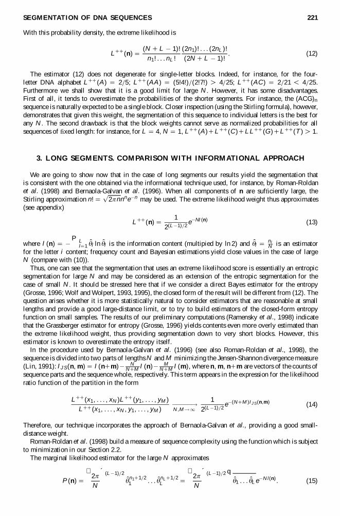
FIG. 3. Histogram of partition probabilities of the E.coli ECCSRASER region.

If one is interested in segmentation on a larger scale, some segments with close compositions should bemerged. In our algorithm, this is done with the help of the partition function.

Generally, the boundaries between long blocks with different compositions correspond to the partitionfunction maxima. However, this probability is a rather smooth function of the sequence position (seediscussion in Section 6), and the inner boundaries of compositionally biased segments close to theirmargins also have relatively high values. Thus, the partition function probabilities should be used withcaution.

In our approach, we calculate the optimal segmentation and then use the partition function to mergeblocks produced by the optimal segmentation. In so doing, the partition function is calculated taking intoaccount only the segmentations obtained by merging the optimal blocks. In this case, the inner boundariesof compositionally biased segments do not obscure the picture.

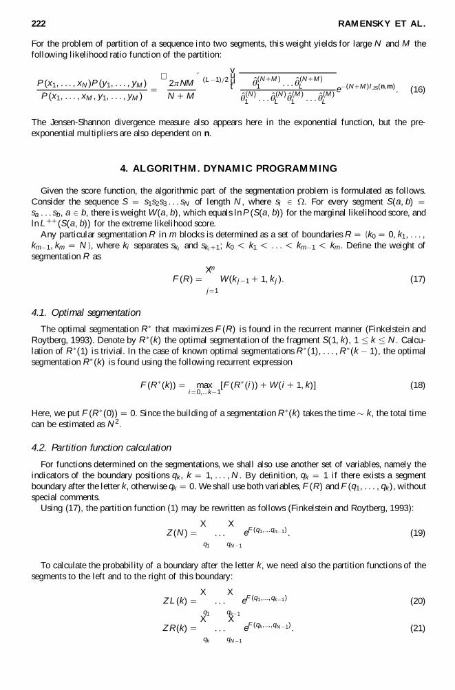
FIG. 4. Histogram of partition probabilities for the boundaries of optimal segmentation of the E. coli ECCSRASERregion.

http://www.liebertonline.com/action/showImage?doi=10.1089/10665270050081487&iName=master.img-000.jpg&w=425&h=218






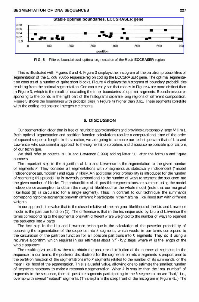
FIG. 5. Filtered boundaries of optimal segmentation of the E.coli ECCRASER region.

This is illustrated with Figures 3 and 4. Figure 3 displays the histogram of the partition probabilities ofsegmentation of the E. coli 708bp sequence region coding the ECCSRASER gene. The optimal segmenta-tion consists of a number of quite short blocks. Figure 4 displays the histogram of boundary probabilitiesresulting from the optimal segmentation. One can clearly see that modes in Figure 4 are more distinct thanin Figure 3, which is the result of excluding the inner boundaries of optimal segments. Boundaries corre-sponding to the points in the right part of the histograms separate long regions of different composition.Figure 5 shows the boundaries with probabilities (in Figure 4) higher than 0.61. These segments correlatewith the coding regions and intergenic elements.

6. DISCUSSION

Our segmentation algorithm is free of heuristic approximations and provides a reasonably large N limit.Both optimal segmentation and partition function calculations require a computational time of the orderof squared sequence length. In this section, we are going to compare our technique with that of Liu andLawrence, who use a similar approach to the segmentation problem, and discuss some possible applicationsof our technique.

We shall refer to objects in Liu and Lawrence (1999) adding letter “L” after the formula and � gurenumbers.

The important step in the algorithm of Liu and Lawrence is the segmentation to the given numberof segments k. They consider all segmentations with k segments as statistically independent (“modelindependence assumption”) and equally likely. An additional prior probability is introduced for the numberof segments; this probability is inversely proportional to the number of ways to segment the sequence intothe given number of blocks. The probabilities of all possible segmentations are summed using the modelindependence assumption to obtain the marginal likelihood for the whole model (note that our marginallikelihood (8) is calculated for a single segment). Thus, in contrast to our technique, the summandscorresponding to the segmentations with different k participate in the marginal likelihood sum with differentweights.

In our approach, the value that is the closest relative of the marginal likelihood of the Liu and Lawrencemodel is the partition function (1). The difference is that in the technique used by Liu and Lawrence theterms corresponding to the segmentations with different k are weighted to the number of ways to segmentthe sequence into k parts.

The � rst step in the Liu and Lawrence technique is the calculation of the posterior probability ofobserving the segmentation of the sequence into k segments, which would in our terms correspond tothe calculation of the partition function for all possible partitions into k segments. They do it using arecursive algorithm, which requires in our estimates about N 2 k=2 steps, where N is the length of thewhole sequence.

The resulting values allow them to obtain the posterior distribution of the number of segments in thesequence. In our terms, the posterior distributions for the segmentation into k segments is proportional tothe partition function of the segmentations into k segments related to the number of its summands, or themean likelihood of the segmentation. This is a useful value, allowing one to estimate the smallest numberof segments necessary to make a reasonable segmentation. When k is smaller than the “real number” ofsegments in the sequence, then all possible segments participating in the k-segmentation are “bad,” i.e.,overlap with several “natural” segments. (This explains the steep front of the histogram in Figure 4L.) The




228 RAMENSKY ET AL.

smooth tail of the distribution appears to be less informative. This agrees with the remark of Stephens(1994), who also considered this problem, that the number of models with different k should be small,and it is generally very dif� cult to make a formal choice between the models. As we do not considerindependent segmentations with different k, we do not calculate this value.

The next value calculated by Liu and Lawrence is the probability that a change point will occur atposition n (19L). Note that probabilities in (19L) are summed without their combinatorial weights, thusthey coincide with our partition functions Z L and Z R , differing only in the normalization.

Using our version of dynamic programming we calculate the numerator much faster (for about k2

(N ¡ k)2 instead of k3 (N ¡ k)3).Moreover, we have observed that probability (2) is of limited use for complicated sequences. The

problem is that expression (2) has high values at all points close to the “true” change point (note thebell-like maxima in Figure 5L). The “true” change points de� nitely correspond to the maxima, but in thecase of a complex sequence, a computer search for the true maxima (excluding probably the several highestones) is rather dif� cult. That is why we use the partition function to � lter the boundaries already producedby the optimal segmentation: the change points between optimal blocks (which as a rule are very short,see Figures 1, 2) are always placed at correct positions as are the change points between the longer blocksafter � ltration.

Liu and Lawrence also obtained several values, such as distribution of boundaries and distribution of thesegmented composition using a sampling procedure. These are important results (especially those related todistribution of the composition). However, it is not clear whether it is possible to obtain reliable samplingresults for a sequence of several thousand base pairs. Since we are more interested in the speci� c positionsof change points rather than in the distributions, we did not use sampling.

We are going now to discuss the possible applications of our segmentation agorithm in biologicalstudies. We believe that it may be applied to every problem in which the nucleic acid composition isimportant. For instance, one can mention the compositional difference between exons and introns, variousdependences in DNA, and RNA composition associated with structural motifs, e.g., loops. Moreover, longeukaryotic genomic regions have been sequenced, so it will be possible to study the isochoric organizationof eukaryotic genes directly. Among other examples of biological problems that can be solved with ourtechnique, we would like to mention the search of gene migration events between genomes with highlydifferent average nucleotide content.

Our technique also may be helpful to calculate the DNA melting curve in thermodynamic experiments.The segmentation obtained can be used for further studies on DNA complexity or fractal structure (Karlin

and Brendel, 1993; Peng et al., 1992). To this end, the distribution of the lengths of homogeneous blocksmay be very informative. Obviously, some, if not a decisive, contribution to the sequence complexitymeasured with various informational measures is explained by the compositional patchiness of the DNAsequence. This patchiness is mostly associated with sense or structural units, exons for instance (Herzel andGrosse, 1997). However, our preliminary studies (Ramensky et al., 1998) indicate that long homogeneoussegments are not necessarily associated with exons and introns and are likely to be of a much broaderorigin. A direct study of the DNA patchiness at the level of full genomes will allow one to understand towhat extent the complexity of DNA is due to compositional patterns, and to what extent it is due to moresubtle correlations.

The investigation of the length distribution of homogeneous segments obtained for long genomic regionswill provide a � nal answer in the discussion on the origin of the fractal dependences in DNA correlationplots (Karlin and Brendel, 1993).

APPENDIX

Marginal and extreme likelihood in the case of large N

Using the Stirling approximation n! 5p

2p nnne ¡ n , it is easy to calculate the form of extreme likelihoodand marginal likelihood for large N . Consider the following fraction:

(N 1 L ¡ 1)!n1! . . . nL !

5(n1 1 . . . 1 nL 1 L ¡ 1)!

n1! . . . nL !. (A1)


The Stirling approximation of the numerator contains the term

(N 1 L ¡ 1)N 1 L ¡ 1 5 N N³

1 1L ¡ 1

N

Ń

(N 1 L ¡ 1)L ¡ 1. (A2)

The second multiplier equals eL ¡ 1 for large N . Then, the direct Stirling approximation of the fraction (A1)is

(N 1 L ¡ 1)!n1! . . . nL !

!

sN L

n1 . . . nL

³N

2p

´(L ¡ 1)=2 ³N

n1

ń1

. . .

³N

nL

ńL

. (A3)

Introducing the point estimator pk 5 nk=N , one can rewrite (A3) as

(N 1 L ¡ 1)!n1! . . . nL !

!³

N

2p

´(L ¡ 1)=2

p ¡ (n11 1=2)1 . . . p ¡ (nL 1 1=2)

L . (A4)

Hence, it is easy to calculate the approximations for the extreme likelihood

(N 1 L ¡ 1)!n1! . . . nL !

(2n1)! . . . (2nL )!

(2N 1 L ¡ 1)!! 2 ¡ (L ¡ 1)=2 pn1

1 . . . pnLL , (A5)

and marginal likelihood.

ACKNOWLEDGMENTS

The authors wish to thank A.M. Leontovich and P.S. Lifanov for their help in the early stage of thiswork, S.R. Sunyaev for useful comments and attention, M.S. Gelfand for his constant interest and fordiscussion on biological applications, D. Haussler for stimulating discussion and for the reference to thework of Liu and Lawrence (1998), and R. Guigo for discussion and for the copy of the proceedings of theHalkidiki (1997) workshop (Lawrence, 1997). The authors thank the anonymous referee for many valuablecomments.

This study has been partially supported by Russian Human Genome Program 18/48 (V.E.R., V.Ju.M.,V.G.T) and 99-0153-F(018) (M.A.R.), RFBR grant N 980448755 and MGRI project 244. M.A.R. is alsosupported by an RFBR Project.

REFERENCES

Bains, W. 1993. Local self-similarity of sequence in mammalian nuclear DNA is modulated by a 180bp periodicity.J. Theor. Biol. 161, 137–143.

Bernaola-Galvan, P., Roman-Roldan, R., and Oliver, J.L. 1996. Compositional segmentation and long-range fractalcorrelation in DNA sequences. Phys. Rev. E. 53(5), 5181–5189.

Bernardi, G. 1989. The isochore organization of the human genome. Ann. Rev. of Gen. 23, 637–661.Bernardi, G. 1995. The human genome: organization and evolutionary history. Ann. Rev. Gen. 29, 445–476.Bernardi, G., Olofson, B., Filipski. J., Zerial. M., Salinas, J. et al. 1985. The mosaic genome of warm-blooded

vertebrate. Science, 228, 953–958.Booth, N.B., and Smith A.F.M. 1992. A Bayesian approach to identi� cation of change-points. J. Econometr. 19, 7–22.Chechetkin, V.R., and Lobzin, V.V. 1998. Study of correlations in segmented DNA sequences: application to structural

coupling between exons and introns. 190, 69–83.Chernoff, H., and Zacks, S. 1964. Estimating the correct mean of a normal distribution which is subjected to a change

in time. Am. Math. Statist., 35, 999–1018.D’Onofrio, G., Mouchiroud D., Aissani B., Gautier C., and Bernardi G. 1991. Correlations between the compositional

properties of human genes, codon usage, and amino acid composition of proteins. J. Mol. Evol. 32, 504–510.Dunbrack, R.L., and Cohen, F.B. 1997. Bayesian statistical analysis of protein side-chain rotamer preferences, Protein

Science, 6, 1661–1681.

230 RAMENSKY ET AL.

Fickett, J.W. 1982. Recognition of protein coding regions in DNA sequences. Nucl. Acid. Res. 10, 5303–5318.Finkelstein, A.V., and Roytberg, M.A. 1993. Computation of biopolymers: A general approach to different problems.

BioSystems, 30, 1–19.Fomin, V.N. 1984. Rekurrentnoe otsenivanie i adaptivnaya � l’tratsiya (Recurrent Inference and Adaptive Filtration).

Moscow, Nauka.Frank, G.K., and Makeev, V.Ju. 1997. G and T nucleotide contents show specie-invariant negative correlation for all

three codon positions. J. Biomol. Str. Dynam. 14, 629–639.Gelfand, M.S. 1992. Statistical analysis and prediction of the exonic structure of human genes. J. Mol. Evol. 35,

239–253.Gelfand, M.S. 1995. Prediction of function in DNA sequence analysis J. Comp. Biol. 2, 87–117.Gelfand, M.S., and Koonin, E.V. 1997. Avoidance of palindromic words in bacterial and archaeal genomes: a close

connection with restriction enzymes. Nucl. Acid. Res. 27, 2430–2439.Grosse, I. 1996. Estimating entropies from � nite samples. Dynamik—Evolution—Strukturen, J. Freund ed., Kosster

Verlag, Berlin, 181–190.Guigo, R., and Fickett, J.W. 1995. Distinctive sequence features in protein coding, genic non-coding and intergenic

human DNA, J. Mol. Biol. 253, 51–60.Herzel, H., and Grosse, I. 1997. Correaltions in DNA sequences: The role of protein coding segments. Phys. Rev. E.

55, 800–810.Karlin, S., and Brendel, V. 1993. Patchiness and correlations in DNA sequences. Science, 259, 677–680.Krogh, A., Brown, M., Mian, S., Sjolander, K., and Haussler, D 1994(a). Protein modeling using hidden Markov

models. J. Mol. Biol. 235, 1501–1531.Krogh, A., Mian, I.S., and Haussler, D. 1994(b). A hidden Markov model that � nds genes in E. coli DNA. Nucl. Acid.

Res. 22, 4768–4778.Kypr, J., and Mrazek, J. 1986. Occurrence of nucleotide triplets in genes and secondary structure of the coded proteins.

Int. J. Biol. Macromol. 9(2), 49–53.Kypr, J., and Mrazek, J. 1995. Middle-range clustering of nucleotides in genomes. Comp. Appl. Bio. Sci. 11, 195–199.Kypr, J., Mrazek, J., and Reich, J. 1989. Nucleotide composition bias and CpG dinucleotide content in the genomes

of HIV and HTLV 1/2. Biochem. Biophys. Acta. 1009, 280–282.Lawrence, C.E. 1997. Bayesian nioinformatics 5th International Conference on Intelligent Systems for Molecular

Biology, Halkidiki-Greece, 1997, 24.Li, W., and Kaneko E. 1992. DNA correlations (scienti� c correspondence) Nature, 360, 635–636.Li, W. 1994. Understanding long-range correlations in DNA sequences. Physica D. 75, 392–416.Li, W. 1997. The study of correlation structure of DNA sequences: A critical review. Computer and Chemistry 21(4),

257–295.Lin, J. 1991. Divergence measures based on the Shannon entropy. IEEE Trans. Inf. Theor. 37, 145–149.Liu, S.L., and Lawrence, C.E. 1998. Bayesian inference on biopolymer models, Stanford Statistical Department

Technical Report (to be published in Journal of Am. Stat. Ass). 24.Liu, S.L., and Lawrence, C.E. 1999 Bayesian inference on biopolymer models, Bioinformatics 15, 38–52.Mrazek, J., and Kypr, J. 1994. Biased distribution of adenine and thymine in gene nucleotide sequences. J. Mol. Evol.

39, 439–447.Ossadnik, S.M., Buldyrev, S.V., Goldberger, A.L., Havlin, S., Mantegna, R.N., Peng, C.-K., Simons, M., and Stanley,

H.E. 1994. Correlation approach to identify coding regions in DNA sequences. Biophysical Journal, 67, 64–70.Peng, C.-K., Buldyrev, S.V., Goldberger, A.L., Havlin, S., Sciortino, F., Simons, M., and Stanley, H.E. 1992. Long-range

correlations in nucleotide sequences. Nature, 356, 168–170.Ramensky, V.E., Makeev, V.Ju., Roitberg, M.A., and Tumanyan, V.G. 1998. Bayesian approach to DNA segmentation.

In: Proceedings of the Theoretical Approach in Biophysics conference. Moscow. Moscow State University.Reese, M.G., Eeckman, F.H., Kulp, D., and Haussler, D. 1997. Improved splice site detection in Genie. J. Comp. Biol.

4:3, 311–323.Roman-Roldan, R., Bernaola-Galvan, P., and Oliver, J.L. 1998. Sequence compositional complexity of DNA through

an entropic segmentation method. Phys. Rev. Lett. 80(4), 1344–1347.Rozanov, Yu.M. 1985. Teoriya veroyatnosti, sluchainye processy i matematicheskaya statistika (Probability Theory,

Stochastic Processes and Mathematical Statistics), Moscow, Nauka.Ryan, M.S., and Nudd, G.R. 1993. The Viterbi algorithm. Warwick Research Report RR238 available via e-mail from

[email protected], K., Karplus, K., Brown, M., Hughey, R., Krogh, A., Mian, I.S., and Haussler, D. 1996. Dirichlet mixtures:

a method for improved detection of weak but signi� cant protein sequence homology. Comput. Appl. Biosci. 12,327–345.

Smith, A.F.M. 1975. A Bayesian approach to inference about a changepoint in a sequence of random variables.Biometrika. 67, 79–84.

Stephens, D.A. 1994. Bayesian retrospective multiple-changepoint identi� cation. Appl. Stat. 43, 159–178.


Sueoka, N. 1959. A statistical analysis of deoxyribonucleic acid distribution in density gradient centrifugation. Proc.Natl. Acad. Sci. 45, 1480–1490.

Trifonov, E.N., and Sussman, J.L. 1980. The pitch of chromatin DNA is re� ected in its nucleotide sequence. Proc.Natl. Acad. Sci. 77(7), 3816–3820.

Tsonis, A.A., Elsner, J.B., and Panagiotis, A. 1991. Periodicity in DNA coding sequences: implication in evolution. J.Theor. Biol. 151, 323–331.

Wolf, D.R., and Wolpert, D.H. 1993. Estimating functions of probability distributions from a � nite set of samples.Part I and II. Los Alamos National Laboratory Report No. LA-UR-93-833 (unpublished). Send emails to [email protected] with subjects “get 9403001” and “get 9403002” to get an encoded postscript version.

Wolpert, D.H., and Wolf, D.R. 1995. Estimating functions of probability distributions from a � nite set of samples.Phys. Rew. E. 52, 6841–6854.

Zazzi, H., Nikosjkov, A., Hall, K., and Luthman, H. 1998. Structural and transcription regulation of the humaninsulin-like growth factor binding protein 4 gene (IGFBP4) Genomics, 49, 401–410

Address correspondence to:V.E. Ramensky

Engelhardt Institute of Molecular BiologyVavilova, 32 Moscow

117984 Russia

E-mail: [email protected]

This article has been cited by:

1. Jie Chen, Ayten Yiğiter, Yu-Ping Wang, Hong-Wen Deng. 2010. A Bayesian Analysis for IdentifyingDNA Copy Number Variations Using a Compound Poisson Process. EURASIP Journal onBioinformatics and Systems Biology 2010, 1-10. [CrossRef]

2. Jonathan M. Keith , Peter Adams , Stuart Stephen , John S. Mattick . 2008. Delineating Slowlyand Rapidly Evolving Fractions of the Drosophila GenomeDelineating Slowly and Rapidly EvolvingFractions of the Drosophila Genome. Journal of Computational Biology 15:4, 407-430. [Abstract][PDF] [PDF Plus]

3. Vivek Thakur, Rajeev Azad, Ram Ramaswamy. 2007. Markov models of genome segmentation.Physical Review E 75:1. . [CrossRef]

4. P L Krapivsky, E Ben-Naim, I Grosse. 2004. Stable distributions in stochastic fragmentation. Journalof Physics A: Mathematical and General 37:8, 2863-2880. [CrossRef]

http://dx.doi.org/10.1155/2010/268513

http://dx.doi.org/10.1089/cmb.2007.0173

http://www.liebertonline.com/doi/pdf/10.1089/cmb.2007.0173

http://www.liebertonline.com/doi/pdfplus/10.1089/cmb.2007.0173

http://dx.doi.org/10.1103/PhysRevE.75.011915

http://dx.doi.org/10.1088/0305-4470/37/8/002

DNA Segmentation Through the Bayesian Approach

Documents