Probabilistic Genotyping Michael D. Coble National Institute of Standards and Technology DNA Mixture Interpretation Webcast April 12, 2013 http://www.nist.gov/oles/forensics/dna-analyst- training-on-mixture-interpretation.cfm http://www.cstl.nist.gov/strbase/mixture.htm

Welcome message from author
This document is posted to help you gain knowledge. Please leave a comment to let me know what you think about it! Share it to your friends and learn new things together.
Transcript

Probabilistic
Genotyping Michael D. Coble
National Institute of Standards and Technology
DNA Mixture Interpretation Webcast
April 12, 2013
http://www.nist.gov/oles/forensics/dna-analyst-
training-on-mixture-interpretation.cfm
http://www.cstl.nist.gov/strbase/mixture.htm

What should we do with discordant data?
• Ignore/drop the locus – this is the “most conservative” option.
A B C
Complainant = AB POI = CD

Curran and Buckleton (2010)
Created 1000 Two-person Mixtures (Budowle et al.1999 AfAm freq.).
Created 10,000 “third person” genotypes.
Compared “third person” to mixture data, calculated PI for included loci,
ignored discordant alleles.

Curran and Buckleton (2010)
30% of the cases had a CPI < 0.01
48% of the cases had a CPI < 0.05
“It is false to think that omitting a locus is
conservative as this is only true if the locus
does not have some exclusionary weight.”

Curran and Buckleton (2010)
POI = C,D
“It is false to think that omitting a locus is conservative as this is
only true if the locus does not have some exclusionary weight.”
A B C D
“Conservative”
Dropping a locus is beneficial to the
“guilty” and detrimental to the “innocent”.

What should we do with discordant
data?
• Ignore/drop the locus – this is the
“most conservative” option.
A B C
Complainant = AB
POI = CD

Suspect
Evidence
Suspect
Evidence
LR 1
2pq =
Suspect
Evidence
“2p”
LR 0
2pq = LR
?
2pq =

Whatever way uncertainty is
approached, probability is the only
sound way to think about it.
-Dennis Lindley
What should we do with discordant
data?
• Continue to use RMNE (CPI, CPE)
• Use the Binary LR with 2p
• Semi-continuous methods with a LR (Drop
models)

Drop Models
• Examine the alleles present and include a Pr(D)
in the LR calculation
A B C
Alleles Present
ABCF

December 2012 Issue of FSI-G

ISFG Recommendations
Pr(D) = Prob. Drop-out (het) Pr(D) = No Prob. Drop-out (het) Pr(D2) = Prob. Drop-out (hom) Pr(D2) = No Prob. Drop-out (hom) Pr(C) = Prob. Drop-in Pr(C) = No Prob. Drop-in

Prosecutor’s Explanation
No Drop-out of the “A” allele The “B” allele dropped out No other Drop-in
Pr(D) Pr(D) Pr(C)

The LR
Pr(D) Pr(D) Pr(C) LR =

Defense Explanation
4 possibilities
(1) The real culprit is a homozygote
pa2Pr(D2) Pr(C)
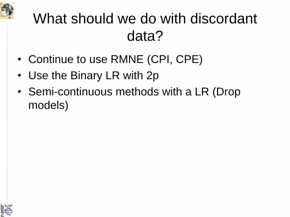
Defense Explanation
4 possibilities
(2) Drop out of a heterozygote (not B) No drop-in of “A”
2papQPr(D)Pr(D)Pr(C)
Q

Defense Explanation
4 possibilities
(3) Drop out of a homozygote (not B) Drop in of “A”
pQ2Pr(D2) Pr(C)pa
Q

Defense Explanation
4 possibilities
(4) Drop out of a homozygote (not AB) Drop in of “A”
2pQpQ’Pr(D)2 Pr(C)pa
Q Q’

The LR
Pr(D) Pr(D) Pr(C) LR =
pa2Pr(D2) Pr(C)
2papQPr(D)Pr(D)Pr(C)
pQ2Pr(D2) Pr(C)pa
2pQpQ’Pr(D)2 Pr(C)pa
+
+
+
Some Drop Model Examples
• LR mix (Haned and Gill)
• Balding and Buckleton (R program)
• FST (NYOCME, Mitchell et al.)
• Kelly et al. (University of Auckland, ESR)
• Lab Retriever (Lohmueller, Rudin and Inman)

What should we do with discordant data?
• Continue to use RMNE (CPI, CPE)
• Use the Binary LR with 2p
• Semi-continuous methods with a LR (Drop models)
• Fully continuous methods with LR

Continuous Models
• Mathematical modeling of “molecular biology” of the profile (mix ratio, PHR (Hb), stutter, etc…) to find optimal genotypes, giving WEIGHT to the results.
A B C
Probable Genotypes AC – 40% BC – 25% CC – 20% CQ – 15%

Some Continuous Model Examples
• TrueAllele (Cybergenetics)
• STRmix (ESR [NZ] and Australia)
• Cowell et al. (FSI-G (2011) 5:202-209)

Challenging Mixture
Michael Donley Dr. Roger Kahn Harris Co. (TX) IFS
CPI = 1 in 1.7*

Challenging Mixture
20, 22 ?
20, 27 ?
20, 20 ? 20, 21 ? ETC…

TrueAllele Results

≈87% major ≈13% minor
Mixture Weight
Bin
Co
un
t

FGA
Inferred – 20,21 Actual – 20,22

Inferred Prob. HWE Suspect
FGA 20, 22 0.1474 0.0543 1
20, 21 0.0722 0.0461 0
20, 26 0.1309 0.0058 0
20, 20 0.0882 0.0156 0
21, 22 0.0056 0.08 0
21, 26 0.0176 0.0085 0
22, 26 0.0077 0.01 0
20, 27 0.0142 0.0008 0
22, 22 0.001 0.0471 0
Statistical Calculation
HP
LR = 0.1474

Inferred Prob. HWE Pr*HWE
FGA 20, 22 0.1474 0.0543 0.008
20, 21 0.0722 0.0461 0.0033
20, 26 0.1309 0.0058 0.0008
20, 20 0.0882 0.0156 0.0014
21, 22 0.0056 0.08 0.0004
21, 26 0.0176 0.0085 0.0001
22, 26 0.0077 0.01 0.0001
20, 27 0.0142 0.0008 0
22, 22 0.001 0.0471 0
0.0143
Statistical Calculation
HD
LR = 0.1474
S
0.0143
LR = 10.33

STRmix


Summary of the Issues
• New kits, new instruments will only increase the
difficulties of interpreting low-level, challenging
samples.
• If we are really serious about properly interpreting low
level and complex mixtures, we must move away from
the RMNE mentality. POPSTATS will not do!!
• Probabilistic methods are the way forward and a
number of software programs are available ranging
from “open source” to commercial packages.

Contact Information
Michael D. Coble
Forensic Biologist
301-975-4330
http://www.cstl.nist.gov/strbase
Thank you for your attention
Additional DNA mixture information available at:
http://www.cstl.nist.gov/strbase/mixture.htm
Related Documents