DKT Dynamic

COMMUNICATIONS IN NUMERICAL METHODS IN ENGINEERINGCommun. Numer. Meth. Engng 2005; 21:651–674Published online 8 June 2005 in Wiley InterScience (www.interscience.wiley.com). DOI: 10.1002/cnm.783

A DKT shell element for dynamic large deformation analysis

Shen Wu1;∗;†, Guangyao Li2 and Ted Belytschko2

1Ford Research Laboratory; Ford Motor Company; 2101 Village Road; SRL-MD 2115;Dearborn; MI 48124; U.S.A.

2Department of Mechanical Engineering; Northwestern University; Evanston; IL 60208; U.S.A.

SUMMARY

The 3-node triangular discrete Kirchho� theory (DKT) element is studied in the context of explicitsoftware for crash analysis. The element uses linear interpolation for the in-plane displacement, quadraticinterpolation for the normal rotations. The transverse displacement has a Hermite cubic interpolationalong element sides. Discrete Kirchho� conditions are imposed at the corner nodes and the sides. Theelement is condensed to �ve degrees-of-freedom per node and can be used with other 3-node and4-node elements. For benchmark example, the DKT element gives good accuracy whereas the 3-nodeC0 element is too sti�. Examples of high-speed component impact analysis demonstrate that DKTelement performs as good as Belytschko–Tsay quadrilateral element, which has been the main elementused for crashworthiness analyses. Copyright ? 2005 John Wiley & Sons, Ltd.

KEY WORDS: discrete Kirchho�; triangular shell element; non-linear �nite element; Reissner–Mindlinplate; explicit �nite element; large deformation

1. INTRODUCTION

Crashworthiness analysis has become an important engineering application of non-linear ex-plicit �nite elements. In most of the applications, the 4-node Belytschko–Tsay quadrilateralelement [1] is used. However, meshing complex shapes such as automobiles with quadri-laterals is often burdensome. Therefore, a considerable incentive exists to develop triangularelements with comparable e�ciency and accuracy. In addition to the meshing di�culties, oneof the drawbacks of the 4-node quadrilateral elements is the modelling of warping. Warpedelements generally occur in any complex geometry. Furthermore, during large bending de-formation, folding may occur along the diagonals of part of the quadrilateral elements andresult in warping, and leads to deterioration in accuracy. On the other hand, for folding along

∗Correspondence to: Shen R. Wu, Ford Research Laboratory, Ford Motor Company, 2101 Village Road, SRL-MD2115, Dearborn, MI 48124, U.S.A.

†E-mail: [email protected]

Received 23 August 2004Revised 5 January 2005

Copyright ? 2005 John Wiley & Sons, Ltd. Accepted 4 March 2005

652 S. WU, G. LI AND T. BELYTSCHKO

one diagonal, the nodal distance along the other diagonal can decrease signi�cantly. Thiseventually causes signi�cant decrease in the stable time step in explicit computations andincrease of computer time. Triangular meshes provide an alternative to avoid these shortcom-ings. However, the direct application of Reissner–Mindlin theory to 3-node C0 shell such asthe LSDYNA triangular element, described in Reference [2], with linear interpolation for allcomponents of displacements and normal rotations, leads to an element that is too sti� andunacceptable except in small areas.As can be seen from linear studies in References [2, 3], among various triangular elements,

the 3-node discrete Kirchho� triangular (DKT) element appears most attractive. The discreteKirchho� approach involves approximations for the normal rotations within the element andindependent description of the transverse displacement on the element boundary. Early de-velopment and application of the discrete Kirchho� theory date back to late 1960s, e.g. seeReferences [4–7]. The DKT element was considered, at that time, as an e�ective elementamong the class of 9-DOF triangular plate bending elements that converge to the Kirchho�thin plate solution. A decade later, in an assessment of plate bending elements with 3-DOFat the corner nodes only, Batoz et al. [8] concluded that the DKT element was still the moste�cient and reliable element of this class. Since then, the DKT plate bending element hasbecome more attractive over other triangular elements, and more developments and applica-tions with DKT elements have been reported, e.g. see References [9–20]. The concept of thediscrete Kirchho� constraint has also been applied to other elements, such as the quadrilateralshell element, see References [11, 21]; the axisymmetric shell element, see Reference [22];for examples of non-linear analysis by the DKT shell, see References [9, 23, 24].By combining the DKT plate bending element with a plane element, various thin shell

elements can be constructed. The simplest element in this family is a 3-node triangle, calledDKT-CST, which combines the DKT plate element for bending and constant strain element(CST) for membrane deformation. Linear and non-linear analyses using DKT-CST shell el-ements can be found in References [9, 24], along with comparisons to other higher-orderquadrilateral shells. Another type of DKT-CST shell element is developed in Reference [3]by using the Marguerre theory and a strain projection to improve membrane behaviour. Onlylinear analysis is performed in Reference [3]. In the current study, the DKT-CST thin shell isimplemented in explicit �nite element software to study its performance in non-linear transientdynamics analysis of large elastic–plastic deformation due to impact.In what follows, we discuss the DKT element formulation and its implementation in an

explicit �nite element code in Section 2. Section 3 is devoted to the numerical examples forassessing the element performance with linear and non-linear test examples, and applicationsof component crash analysis, followed by concluding remarks in Section 4.

2. DKT FOR EXPLICIT FINITE ELEMENT

In this section, we describe the 3-node triangular shell element based on the discrete Kirchho�plate theory. The curved shell structure is approximated by piecewise �at surface segments.This element uses co-rotational formulation, described in Reference [25], which is applicableto large displacements, �nite rotation and small strain increment. For illustration, an elementlocal co-ordinate system can be de�ned such that x3 is normal to the element plane, as shownin Figure 1. The following discussion of element formulation will be referred to this local

Copyright ? 2005 John Wiley & Sons, Ltd. Commun. Numer. Meth. Engng 2005; 21:651–674

DKT SHELL ELEMENT 653

4

1

3

6

5

x1

x2 3

1

2

e1

e2

5 4

6

η•

•

••

•

•

•

•

•

••

•

ξ2

Figure 1. Triangular element in a local system and the master element.

v1

2

z

x3

v2

1

x3

ωω

ω

2zω1

Figure 2. Velocity representation of Reissner–Mindlin plate.

system. It is understood that a transformation to a global system is necessary for elementassembly and the formation of the system equations.For the explicit �nite element method, an incremental approach is used. At each time

step, the strain increments are calculated from the gradients of nodal velocities and angularvelocities. Then the stress increments are calculated from strain increments by the constitutivelaws.For the Reissner–Mindlin plate, the velocity components of a generic point in the shell is

represented by the velocities and the normal rotational velocities (the angular velocities) atmid-surface, as shown in Figure 2,

V1 = v1 + z!2

V2 = v2 − z!1

V3 = v3

(1)

where ‘z’ represents the distance from the generic point to the mid-surface. The normal isassumed straight, but is not necessary to keep orthogonal to the mid-surface after deformation.Here, v1, v2, v3, !1 and !2 are functions of (t; x; y). The transverse shear strain rates �13 and�23 depend on the velocity v3 and the normal rotational velocities !1 and !2 only. We alsouse the notation �=!1e1 + !2e2 and S= �13e1 + �23e2. These variables are all expressed inco-rotational components.



The 3-node linear interpolation is employed for the in-plane velocities v1 and v2, e.g. seeReference [26],

’1 = 1− � − �

’2 = �

’3 = �

(2)

A 6-node quadratic interpolation is used for the angular velocities !1 and !2 (2× 6=12unknowns),

!1 =6∑

J=1!J1 J (�; �)

!2 =6∑

J=1!J2 J (�; �)

(3)

On the master (parametric) element, shown in Figure 1, the shape functions are

1 = (1− � − �)(1− 2� − 2�) 2 = �(2� − 1) 3 = �(2� − 1) 4 = 4��

5 = 4�(1− � − �)

6 = 4�(1− � − �)

(4)

For the transversal velocity v3, the element uses 2-node Hermite cubic interpolation alongeach of the three sides (3× 4− 3=9 unknowns). For example, using parameter s from 0 to1 along side 1 with nodes 1 and 2, we have

v3|Side 1 = v13�1 + v23�2 + (v3; S )1�11 + (v3; S )

2�12 (5)

�1 = 1− 3s2 + 2s3

�2 = 3s2 − 2s3

�11 = (s − 2s2 + s3)L (6)

�12 = (−s2 + s3)L

The following discrete Kirchho� constraints are then imposed on a set of speci�c points,similar to what is described in Batoz [10]:

(H1) �13 = �23 = 0 at three corner nodes (2× 3 conditions);(H2) The normal components of the transverse shear strain rate �n=0 at three mid-points

of the sides (3 conditions).



x1

x2

1

2

e1

e2

6

n

s

x1

x3 3

1

2 5

4

6

x2v3

ωn

α

•

••

•

•

•

•

•

•

•

•

Figure 3. Geometry at the side.

In addition, we require(H3) The tangential components of angular velocity !t are linear along three sides

(3 conditions).In fact, condition (H1) is equivalent to the Kirchho� conditions applied to the com-ponents normal to the sides, at both ends on the three sides, illustrated in Figure 3.

So far, we have introduced 21 unknowns in Equations (3) and (5) and imposed 12 con-ditions in (H1–H3) related to the transverse velocity and the angular velocities. Thus, weexpect to have a reduced system with nine independent unknowns, just three per node.As a matter of fact, conditions (H1) and (H2) can be expressed as, with L to be the length

of the side,

!n=@v3@l=

@v3L@s

at s=0; 0:5; 1 of each side (7)

For side 1, with nodes 1, 6, and 2, we have, in view of (6)

!1n =@v3L@s

∣∣∣∣S=0

= (v3; S )1

!2n =

@v3L@s

∣∣∣∣S=1

= (v3; S )2

!6n =@v3L@s

∣∣∣∣S=0:5

= 1:5(v23 − v13)=L − 0:25((v3; S )1 + (v3; S )2)

= 1:5(v23 − v13)=L − 0:25(!1n +!2n)

(8)

Condition (H3) states that the tangential component of the angular velocity at mid-side nodeequal to the average angular velocity of the end nodes, i.e.

!6S =(!1S +!2S)=2 (9)

Using Equations (8) and (9), with the 2-D vector form, we have

�6 =!61e1 +!62e2 =!6SeS +!6nen

=0:5(!1S +!2S)es + (1:5(v23 − v13)=L − 0:25(!1n +!2n))en

=0:5(�1 + �2) + (1:5(v23 − v13)=L − 0:75(!1n +!2n))en (10)



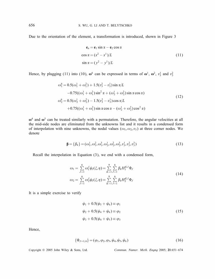
Due to the orientation of the element, a transformation is introduced, shown in Figure 3

en = e1 sin � − e2 cos �cos �= (x2 − x1)=L

sin �= (y2 − y1)=L

(11)

Hence, by plugging (11) into (10), �6 can be expressed in terms of �1, �2, v13 and v23

!61 = 0:5(!11 +!21) + 1:5(v

23 − v13) sin �=L

−0:75((!11 +!21) sin2 �+ (!12 +!22) sin � cos �)

!62 = 0:5(!12 +!22)− 1:5(v23 − v13) cos �=L

+0:75((!11 +!21) sin � cos � − (!12 +!22) cos2 �)

(12)

�4 and �5 can be treated similarly with a permutation. Therefore, the angular velocities at allthe mid-side nodes are eliminated from the unknowns list and it results in a condensed formof interpolation with nine unknowns, the nodal values (!1; !2; v3) at three corner nodes. Wedenote

R= {�k}=(!11; !21; !31; !12; !22; !32; v13; v23 ; v33) (13)

Recall the interpolation in Equation (3), we end with a condensed form,

!1 =6∑

J=1!J1 J (�; �)=

9∑K=1

6∑J=1

�kHKJ1 �J

!2 =6∑

J=1!J2 J (�; �)=

9∑K=1

6∑J=1

�kHKJ2 �J

(14)

It is a simple exercise to verify

1 + 0:5( 5 + 6)≡ ’1

2 + 0:5( 4 + 6)≡ ’2

3 + 0:5( 4 + 5)≡ ’3

(15)

Hence,

{�J=1;6}=(’1; ’2; ’3; 4; 5; 6) (16)



We summarize with the following condensation coe�cients H -matrix:

(HKJ1 )K=1;9; J=1;6 =

⎡⎢⎢⎢⎢⎢⎢⎢⎢⎢⎢⎢⎢⎢⎢⎢⎢⎢⎢⎢⎢⎢⎢⎢⎢⎣

[I3]

⎡⎢⎢⎣

0 −SS2 −SS3

−SS1 0 −SS3

−SS1 −SS2 0

⎤⎥⎥⎦

[O3]

⎡⎢⎢⎣0 SC2 SC3

SC1 0 SC3

SC1 SC2 0

⎤⎥⎥⎦

[O3]

⎡⎢⎢⎣

0 SL2 −SL3

−SL1 0 SL3

SL1 −SL2 0

⎤⎥⎥⎦

⎤⎥⎥⎥⎥⎥⎥⎥⎥⎥⎥⎥⎥⎥⎥⎥⎥⎥⎥⎥⎥⎥⎥⎥⎥⎦

(17a)

(HKJ2 )K=1;9; J=1;6 =

⎡⎢⎢⎢⎢⎢⎢⎢⎢⎢⎢⎢⎢⎢⎢⎢⎢⎢⎢⎢⎢⎢⎢⎣

[O3]

⎡⎢⎢⎣0 SC2 SC3

SC1 0 SC3

SC1 SC2 0

⎤⎥⎥⎦

[I3]

⎡⎢⎢⎣

0 −CC2 −CC3

−CC1 0 −CC3

−CC1 −CC2 0

⎤⎥⎥⎦

[O3]

⎡⎢⎢⎣

0 −CL2 CL3

CL1 0 −CL3

−CL1 CL2 0

⎤⎥⎥⎦

⎤⎥⎥⎥⎥⎥⎥⎥⎥⎥⎥⎥⎥⎥⎥⎥⎥⎥⎥⎥⎥⎥⎥⎦

(17b)

where I3 and O3 are the third-order identity matrix and zero matrix, respectively. Otherparameters are de�ned below, with �i the orientation angle of side i as shown in Figure 3and Li the length of side i,

SSi =0:75 sin2 �i

CCi =0:75 cos2 �i

SCi =0:75 sin �i cos �i

SLi =1:5 sin �i=Li

CLi =1:5 cos �i=Li

(18)



The above su�ces for the implementation in the explicit software, without the need toform a sti�ness matrix. At each time step, we calculate increments of deformation, strain andstress of the element. The nodal force and moment are obtained by numerical integrationsthrough the thickness. Due to the use of higher-order interpolation, quadrature with multipleintegration points for in-plane integration is recommended. As well known, one point (atcentre) scheme can only accurately integrate up to the linear polynomials. A 3-point schemecan accurately integrate up to the complete second-degree polynomials. A 2-point scheme canaccurately integrate up to the linear polynomials, but nearly accurate for the second-degreepolynomials. Preliminary results of DKT elements using 2-point integration are presented inReference [27]. Thus, the membrane part can use one point scheme and the bending part canuse 3-point or 2-point scheme.

3. NUMERICAL EXAMPLES

3.1. Twisted beam

The twisted beam example is often used to verify the ability of the shell element toobtain correct response when the shell is warped, e.g. Reference [28]. The example, de�ned inReference [29], is described in Figure 4 with a 12× 2(× 2) mesh. A speci�ed load is appliedat one end and clamped boundary condition is imposed at the other end. So, it is like acantilever beam. The linear static solution of displacement at the tip is 0.005424, the maxi-mum of dynamic response at the tip is to be double. The computed displacement time historyof the tip point, by using various types of elements with the 12× 2 mesh, is shown inFigure 5(a). It is observed that DKT element and quadrilateral QPH element [30] give thesame accurate results. As described in Reference [30], a drill projection is used for QPH ele-ment. Without this projection, the result will diverge immediately. The 4-node B–T shell withreduced integration [1], commonly used in crashworthiness analysis, does not give answer tothis example. The reason is mainly the hour glassing caused by warping due to quadrilateralmeshing of the curved surface. In this example, warping exists everywhere. It should be noted

Length =12.0 Width =1.1 Thickness = 0.32 E = 2.9e7

F= 1.0

F

clamped

ν = 0.22 ρ = 2.5e-4

Figure 4. Twisted beam.



Figure 5. Displacement at the end point of the twisted beam: (a) solutions from various elements;and (b) solutions from DKT elements with various element sizes.



Radius = 10.0 Thickness = 0.04 E = 6.825e7 ν = 0.3 ρ = 2.5e-4

F = 1.0

F

F

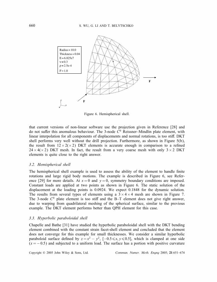
Figure 6. Hemispherical shell.

that current versions of non-linear software use the projection given in Reference [28] anddo not su�er this anomalous behaviour. The 3-node C0 Reissner–Mindlin plate element, withlinear interpolation for all components of displacements and normal rotations, is too sti�. DKTshell performs very well without the drill projection. Furthermore, as shown in Figure 5(b),the result from 12× 2(× 2) DKT elements is accurate enough in comparison to a re�ned24× 4(× 2) DKT mesh. In fact, the result from a very coarse mesh with only 3× 2 DKTelements is quite close to the right answer.

3.2. Hemispherical shell

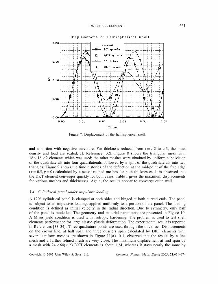
The hemispherical shell example is used to assess the ability of the element to handle �niterotations and large rigid body motions. The example is described in Figure 6, see Refer-ence [29] for more details. At x=0 and y=0, symmetry boundary conditions are imposed.Constant loads are applied at two points as shown in Figure 6. The static solution of thedisplacement at the loading points is 0.0924. We expect 0.1848 for the dynamic solution.The results from several types of elements using a 3× 4× 4 mesh are shown in Figure 7.The 3-node C0 plate element is too sti� and the B–T element does not give right answer,due to warping from quadrilateral meshing of the spherical surface, similar to the previousexample. The DKT element performs better than QPH element for this case.

3.3. Hyperbolic paraboloidal shell

Chapelle and Bathe [31] have studied the hyperbolic paraboloidal shell with the DKT bendingelement combined with the constant strain facet-shell element and concluded that the elementdoes not converge for this example for small thicknesses. We consider a similar hyperbolicparaboloid surface de�ned by z= x2 − y2, [−0:56x; y60:5], which is clamped at one side(x=− 0:5) and subjected to a uniform load. The surface has a portion with positive curvature



Figure 7. Displacement of the hemispherical shell.

and a portion with negative curvature. For thickness reduced from t=e-2 to e-3, the massdensity and load are scaled, cf. Reference [32]. Figure 8 shows the triangular mesh with18× 18× 2 elements which was used; the other meshes were obtained by uniform subdivisionof the quadrilaterals into four quadrilaterals, followed by a split of the quadrilaterals into twotriangles. Figure 9 shows the time histories of the de�ection at the mid-point of the free edge(x=0:5; y=0) calculated by a set of re�ned meshes for both thicknesses. It is observed thatthe DKT element converges quickly for both cases. Table I gives the maximum displacementsfor various meshes and thicknesses. Again, the results appear to converge quite well.

3.4. Cylindrical panel under impulsive loading

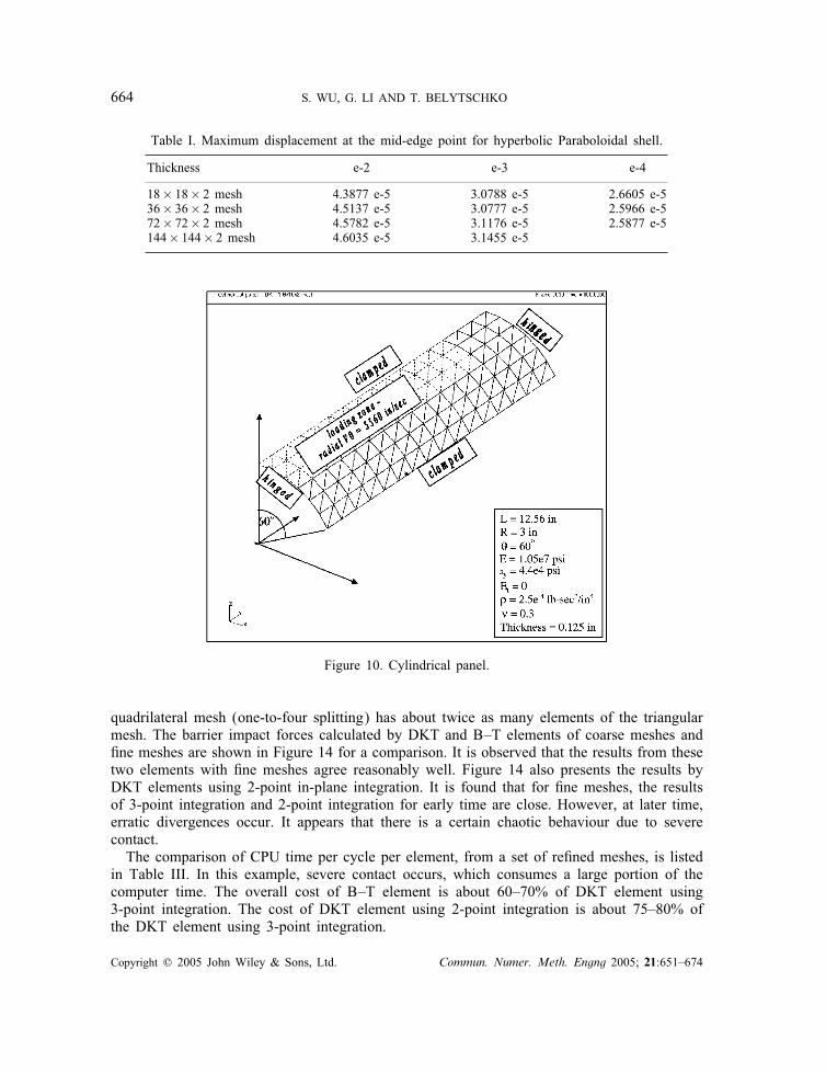
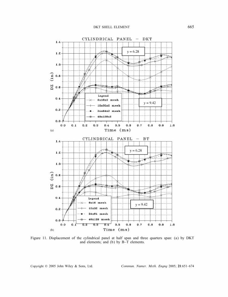
A 120◦ cylindrical panel is clamped at both sides and hinged at both curved ends. The panelis subject to an impulsive loading, applied uniformly to a portion of the panel. The loadingcondition is de�ned as initial velocity in the radial direction. Due to symmetry, only halfof the panel is modelled. The geometry and material parameters are presented in Figure 10.A Mises yield condition is used with isotropic hardening. The problem is used to test shellelements performance for large elastic–plastic deformation. The experimental result is reportedin References [33, 34]. Three quadrature points are used through the thickness. Displacementson the crown line, at half span and three quarters span calculated by DKT elements withseveral uniform meshes are shown in Figure 11(a). It is observed that the results by a �nemesh and a further re�ned mesh are very close. The maximum displacement at mid span bya mesh with 24× 64(× 2) DKT elements is about 1.24, whereas it stays nearly the same by



Figure 8. Triangular mesh for the hyperbolic paraboloid.

a re�ned mesh with 48× 128(× 2) elements. This is close to the experimental data near 1.25,cf. References [33, 34]. The maximum displacement at three quarters span by DKT elementsis about 0.64, whereas the experimental result in Reference [33] is around 0.72. For thisexample, when mesh is �ne, the results by B–T elements, shown in Figure 11(b), are veryclose to those by DKT elements.In this example, large deformation occurs, but without surface contact. The computer time

is almost entirely in nodal force evaluation of the element procedure. The CPU time per cycleper element using DKT elements is compared to B–T quadratic elements in Table II. Theresults are given for a set of re�ned meshes. The cost of B–T element is about 50–70% ofthe DKT element using 3-point in-plane integration. When using 2-point integration, the costof DKT element is reduced to 65–85%.

3.5. Crash can

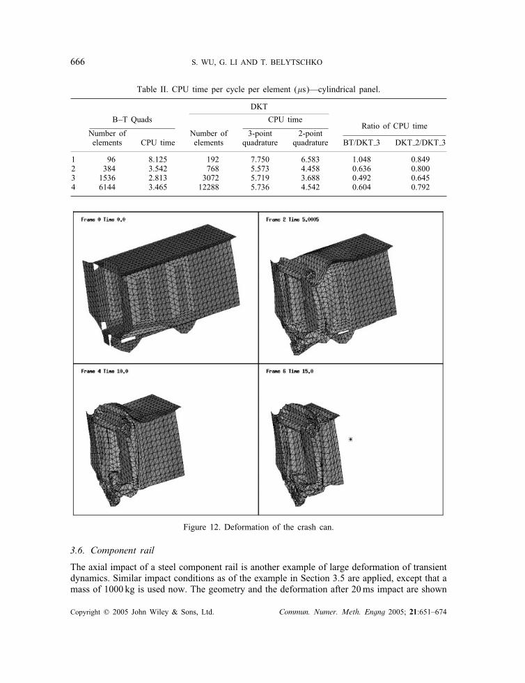
The axial crash simulation for an aluminium component, the crash can, is studied to comparethe performance of DKT elements and quadrilateral elements in dynamic large deformationapplications. The crash can impacts into a rigid barrier with an initial velocity of 15mm=msand an attached mass of 500 kg. Convolutions are designed to lead the large deformationinto a desired progressive collapse mode. The component geometry and the deformationafter 15ms impact are shown in Figure 12. The internal energy calculated from severaluniformly re�ned meshes of DKT elements and B–T quadrilateral elements is shown inFigure 13. When examining the di�erence in internal energy calculated from coarse meshes



Figure 9. Displacement at mid-point of the free edge (x=0:5; y=0): (a) t=e-2; and (b) t=e-3.

and �ne meshes, we observe that the results of DKT elements have less di�erence than those ofB–T elements. Regarding element size, the result of a triangular mesh from split of a quadsmesh is comparable to a quadrilateral mesh from uniform re�nement. In this case, re�ned



Table I. Maximum displacement at the mid-edge point for hyperbolic Paraboloidal shell.

Thickness e-2 e-3 e-4

18× 18× 2 mesh 4.3877 e-5 3.0788 e-5 2.6605 e-536× 36× 2 mesh 4.5137 e-5 3.0777 e-5 2.5966 e-572× 72× 2 mesh 4.5782 e-5 3.1176 e-5 2.5877 e-5144× 144× 2 mesh 4.6035 e-5 3.1455 e-5

Figure 10. Cylindrical panel.

quadrilateral mesh (one-to-four splitting) has about twice as many elements of the triangularmesh. The barrier impact forces calculated by DKT and B–T elements of coarse meshes and�ne meshes are shown in Figure 14 for a comparison. It is observed that the results from thesetwo elements with �ne meshes agree reasonably well. Figure 14 also presents the results byDKT elements using 2-point in-plane integration. It is found that for �ne meshes, the resultsof 3-point integration and 2-point integration for early time are close. However, at later time,erratic divergences occur. It appears that there is a certain chaotic behaviour due to severecontact.The comparison of CPU time per cycle per element, from a set of re�ned meshes, is listed

in Table III. In this example, severe contact occurs, which consumes a large portion of thecomputer time. The overall cost of B–T element is about 60–70% of DKT element using3-point integration. The cost of DKT element using 2-point integration is about 75–80% ofthe DKT element using 3-point integration.



Figure 11. Displacement of the cylindrical panel at half span and three quarters span: (a) by DKTand elements; and (b) by B–T elements.



Table II. CPU time per cycle per element (�s)—cylindrical panel.

DKT

B–T Quads CPU timeRatio of CPU time

Number of Number of 3-point 2-pointelements CPU time elements quadrature quadrature BT/DKT 3 DKT 2/DKT 3

1 96 8.125 192 7.750 6.583 1.048 0.8492 384 3.542 768 5.573 4.458 0.636 0.8003 1536 2.813 3072 5.719 3.688 0.492 0.6454 6144 3.465 12288 5.736 4.542 0.604 0.792

Figure 12. Deformation of the crash can.

3.6. Component rail

The axial impact of a steel component rail is another example of large deformation of transientdynamics. Similar impact conditions as of the example in Section 3.5 are applied, except that amass of 1000 kg is used now. The geometry and the deformation after 20ms impact are shown



Figure 13. Internal energy of the crash can: (a) results from DKT meshes;and (b) results from B–T quads meshes.



Figure 14. Barrier impact force of the crash can: (a) results from the coarse meshes;and (b) results from the �ne meshes.



Table III. CPU time per cycle per element (�s)—crash can.

DKT



1 565 4.497 1027 7.279 5.558 0.618 0.7642 2260 4.655 4108 7.379 5.882 0.631 0.7973 9040 5.111 16432 7.417 5.951 0.689 0.8024 36160 5.258 65728 7.347 5.946 0.716 0.809

Figure 15. Deformation of the rail.

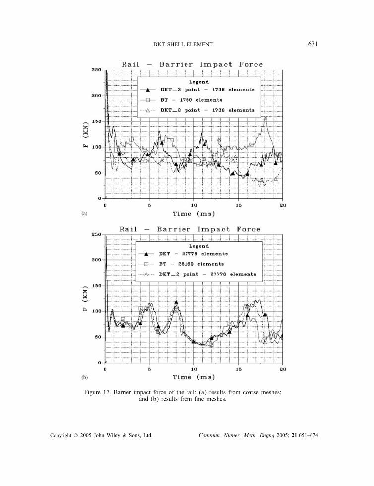
in Figure 15. The internal energy calculated from several re�ned meshes of DKT elementsand B–T quadrilateral elements is shown in Figure 16. The barrier impact force is shownin Figure 17. The coarse triangular mesh used in this example is split from the quadrilateralmesh in a one-to-four cross pattern. All re�ned meshes are generated from the coarse meshes



Figure 16. Internal energy of the rail: (a) results from DKT meshes;and (b) results from B–T quads meshes.

by further splitting one into four. Therefore, the triangular meshes have almost same numberof elements as the correspondingly re�ned quadrilateral meshes. It is observed from Figure 16,for the quadrilateral meshes, the di�erence in internal energy from a coarse mesh and the �nermeshes is signi�cant. The di�erence from triangular meshes is less. On the other hand, for



Figure 17. Barrier impact force of the rail: (a) results from coarse meshes;and (b) results from �ne meshes.



Table IV. CPU time per cycle per element (�s)—rail.

DKT



1 440 4.121 434 7.408 5.984 0.556 0.8082 1760 3.934 1736 6.711 4.991 0.586 0.7443 7040 4.698 6944 6.830 5.425 0.688 0.7944 28160 5.093 27776 6.993 5.701 0.728 0.8155 112640 4.886 111104 6.545 5.337 0.743 0.815

�ne meshes, the di�erences in the results for both internal energy and barrier impact forcefrom quadrilateral mesh and triangular mesh become quite small. Figure 17 also presents theresults by DKT elements using 2-point in-plane integration. It is found, that for �ne meshes,the results of 3-point integration and 2-point integration are close for early time. However, forall cases, late time results do not appear to converge, probably because of e�ects of discretecontact.The comparison of CPU time per cycle per element, from a set of re�ned meshes, is

listed in Table IV. In this example, severe contact happens, which consumes a portion of thecomputer time. The overall cost of B–T element is about 55–70% of DKT element using3-point integration. The cost of DKT element using 2-point integration is about 75–80% ofthe DKT element using 3-point integration.

4. CONCLUDING REMARKS

The implementation of a 3-node discrete Kirchho� element in explicit �nite element softwarewas described. Simpli�ed formulas that reduce computer time are given. It is shown that theresulting element is comparable in running time to the B–T one-point quadrature element.The examples of a twisted beam and a hemispherical shell showed that the DKT element hadaccurate solution whereas the B–T quadrilateral element did not give right solution, due towarping induced by quadrilateral meshing, and the simple 3-node C0 element was too sti�.The example of a hyperbolic paraboloid clamped at one edge, subject to uniform loadingshowed that the DKT element converged quickly, even with reduced thickness. Elastic–plasticdeformation of a cylindrical panel subject to impulsive loading, and two examples of compo-nent axial impact demonstrated the applications of the DKT elements to non-linear dynamicproblems. The comparison with the quadrilateral B–T element showed that, from coarse meshto �ne mesh, the di�erence of the internal energy calculated by DKT elements was lessthan that by B–T quadrilateral elements. It was also observed that the results by �ne meshesof DKT elements, both using 3-point in-plane integration or 2-point integration, and B–Tquadrilateral elements were close.Triangular elements are very attractive to industry because they simplify meshing. The

accuracy of the results is comparable to the Belytschko–Tsay [1] in situations when the later



is convergent, and comparable to the physically stabilized QPH [30]. Running time is onlyslightly greater. Thus, the performance of the element is quite promising.

REFERENCES

1. Belytschko T, Lin JL, Tsay CS. Explicit algorithms for the nonlinear dynamics of shells. Computer Methodsin Applied Mechanics and Engineering 1984; 42:225–251.

2. Carpenter N, Stolarski H, Belytschko T. A �at triangular shell element with improved membrane interpolation.Communications in Applied Numerical Methods 1985; 1:161–168.

3. Carpenter N, Stolarski H, Belytschko T. Improvements in 3-node triangular shell elements. International Journalfor Numerical Methods in Engineering 1986; 23:1643–1667.

4. Wempner GA, Oden JT, Kross DA. Finite element analysis of thin shells. Journal of the Engineering MechanicsDivision, Proceedings of the American Society of Civil Engineers 1968; 94:1273–1294.

5. Stricklin JA, Haisler WE, Tisdale PR, Gunderson R. A rapidly converging triangular plate element. AIAAJournal 1969; 7:180–181.

6. Dhatt G. Numerical analysis of thin shells by curved triangular elements based on discrete Kirchho� hypothesis.Proceedings of the ASCE Symposium on Applications of FEM in Civil Engineering 1969; 13–14.

7. Dhatt D. An e�cient triangular shell element. AIAA Journal 1970; 8:2100–2102.8. Batoz JL, Bathe KJ, Ho LW. A study of three-node triangular plate bending element. International Journal forNumerical Methods in Engineering 1980; 15:1771–1812.

9. Bathe KJ, Ho LW. A simple and e�ective element for analysis of general shell structures. Computers andStructures 1981; 13:673–681.

10. Batoz JL. An explicit formulation for an e�cient triangular plate-bending element. International Journal forNumerical Methods in Engineering 1982; 18:1077–1089.

11. Batoz JL, Tahar MB. Evaluation of a new quadrilateral thin plate bending element. International Journal forNumerical Methods in Engineering 1982; 18:1655–1677.

12. Murthy SS, Gallagher RH. Anisotropic cylindrical shell element based on discrete Kirchho� theory. InternationalJournal for Numerical Methods in Engineering 1983; 19:1805–1823.

13. Jeyachandrabose C, Kirkhope J, Babu CR. An alternative explicit formulation for the DKT plate-bending element.International Journal for Numerical Methods in Engineering 1985; 21:1289–1293.

14. Jeyachandrabose C, Kirkhope J. Construction of new e�cient three-node triangular thin plate bending elements.Computers and Structures 1986; 23:587–603.

15. Batoz JL, Lardeur P. A discrete shear triangular nine D.O.F. element for the analysis of thick to very thin plate.International Journal for Numerical Methods in Engineering 1989; 28:533–560.

16. Fafard M, Dhatt G, Batoz JL. A new discrete Kirchho� plate=shell element with updated procedures. Computersand Structures 1989; 31:591–606.

17. Batoz JL, Katili I. On a simple triangular Reissner–Mindlin plate element based on incompatible modes anddiscrete constrains. International Journal for Numerical Methods in Engineering 1992; 35:1603–1632.

18. Katili I. A new discrete Kirchho�–Mindlin element based on Mindlin–Reissner plate theory and assumed shearstrain �elds—Part I: an extended DKT element for thick-plate bending analysis. International Journal forNumerical Methods in Engineering 1993; 36:1859–1883.

19. Katili I. A new discrete Kirchho�–Mindlin element based on Mindlin–Reissner plate theory and assumed shearstrain �elds—Part II: an extended DKQ element for thick-plate bending analysis. International Journal forNumerical Methods in Engineering 1993; 36:1885–1908.

20. Li KP, Habraken AM, Bruneel H. Simulation of square cup deep drawing with di�erent �nite elements.Proceedings of NUMISHEET’93 Conference, 1993.

21. Jeyachandrabose C, Kirkhope J, Meekisho L. An improved discrete Kirchho� quadrilateral thin-plate bendingelement. International Journal for Numerical Methods in Engineering 1987; 24:635–654.

22. Weeks GE. A �nite element model for shells based on the discrete Kirchho� hypothesis. International Journalfor Numerical Methods in Engineering 1972; 5:3–16.

23. Bathe KJ, Dvorkin E, Ho LW. Our discrete Kirchho� and isoparametric shell elements for nonlinear analysis—anassessment. Computers and Structures 1983; 16:89–98.

24. Wenzel T, Schoop H. A nonlinear triangular curved shell element. Communications in Numerical Methods inEngineering 2004; 20:251–264.

25. Belytschko T, Hsieh BJ. Nonlinear transient �nite element analysis with convected co-ordinates. InternationalJournal for Numerical Methods in Engineering 1973; 7:255–271.

26. Belytschko T, Stolarski H, Carpenter N. A C0 triangular plate element with one-point quadrature. InternationalJournal for Numerical Methods in Engineering 1984; 20:787–802.

27. Li G, Belytschko T, Wu SR. Performance of DKT thin shell element with 2 point integration scheme for largedeformation analysis. Proceedings of the 6th U.S. National Congress of Computational Mechanics, 2001.



28. Belytschko T, Wong BL, Chiang HY. Advances in one-point quadrature shell elements. Computer Methods inApplied Mechanics and Engineering 1992; 96:93–107.

29. MacNeal RH, Harder RL. A proposed standard set of problems to test �nite element accuracy. Finite Elementin Analysis and Design 1985; 1:3–20.

30. Belytschko T, Leviathan I. Physical stabilization of 4-node shell element with one-point quadrature. ComputerMethods in Applied Mechanics and Engineering 1994; 113:321–350.

31. Chapelle D, Bathe KJ. The Finite Element Analysis of Shells—Fundamentals. Springer: Berlin, 2003.32. Wu SR. Reissner–Mindlin plate theory for elastodynamics. Journal of Applied Mathematics 2004; 2004:

179–189.33. Balmer HA, Witmer EA. Theoretical–experimental correlation of large dynamic and permanent deformatins

of impulsively loaded simple structures. Massachusetts Institute of Technology, Aeroelastic and StructuresResearch Laboratory, FDL-TDR-64-108, July 1964.

34. Morino L, Leech JW, Witmer EA. An improved numerical calculation technique for large elastic–plastic transientdeformations of thin shells. Part 2—evaluation and applications. Journal of Applied Mechanics, Transactionsof ASME 1971; 38:429–436.


DKT Dynamic

Documents