Divide and Conquer - courses.cs.washington.edu · 3 Fast Fourier Transform: Applications Applications. Optics, acoustics, quantum physics, telecommunications, control systems, signal

1

Chapter 5 Divide and Conquer

Slides by Kevin Wayne. Copyright © 2005 Pearson-Addison Wesley. All rights reserved.

Addition/modifications by P. Beame, W.L. Ruzzo

5.6 Convolution and FFT

3

Fast Fourier Transform: Applications

Applications.   Optics, acoustics, quantum physics, telecommunications, control

systems, signal processing, speech recognition, data compression, image processing.

  DVD, JPEG, MP3, MRI, CAT scan.   Numerical solutions to Poisson's equation.

The FFT is one of the truly great computational developments of this [20th] century. It has changed the face of science and engineering so much that it is not an exaggeration to say that life as we know it would be very different without the FFT. -Charles van Loan

4

Fast Fourier Transform: Brief History

Gauss (1805, 1866). Analyzed periodic motion of asteroid Ceres. Runge-König (1924). Laid theoretical groundwork. Danielson-Lanczos (1942). Efficient algorithm. Cooley-Tukey (1965). Monitoring nuclear tests in Soviet Union and tracking submarines. Rediscovered and popularized FFT.

Importance not fully realized until advent of digital computers.

5

Polynomials: Coefficient Representation

Polynomial. [coefficient representation]

Add: O(n) arithmetic operations. Evaluate: O(n) using Horner's method. Multiply (convolve): O(n2) using brute force.

€

A(x) = a0 + a1x + a2x2 ++ an−1x

n−1

€

B(x) = b0 +b1x +b2x2 ++ bn−1x

n−1

€

A(x)+ B(x) = (a0 +b0 )+ (a1 +b1)x ++ (an−1 +bn−1)xn−1

€

A(x) = a0 + (x (a1 + x (a2 ++ x (an−2 + x (an−1))))

€

A(x)× B(x) = ci xi

i =0

2n−2∑ , where ci = a j bi− j

j =0

i

∑

6

Polynomials: Point-Value Representation

Fundamental theorem of algebra. [Gauss, PhD thesis] A degree n polynomial with complex coefficients has n complex roots. Corollary. A degree n-1 polynomial A(x) is uniquely specified by its evaluation at n distinct values of x.

x

y

xj

yj = A(xj)

7

Polynomials: Operations on Point-Value Representation

Polynomial. [point-value representation] Add: O(n) arithmetic operations. Multiply: O(n), but need 2n-1 points.

Evaluate: O(n2) using Lagrange's formula.

€

A(x) : (x0, y0 ), …, (xn-1, yn−1) B(x) : (x0, z0 ), …, (xn-1, zn−1)

€

A(x)+ B(x) : (x0, y0 + z0 ),…, (xn-1, yn−1 + zn−1)

€

A(x) = yk

(x − x j )j≠k∏

(xk − x j )j≠k∏k=0

n−1∑

€

A(x) × B(x) : (x0, y0 × z0 ),…, (x2n-1, y2n−1× z2n−1)

8

Converting Between Two Polynomial Representations

Tradeoff. Fast evaluation or fast multiplication. We want both! Goal. Make all ops fast by efficiently converting between two representations.

Coefficient

Representation

O(n2)

Multiply

O(n)

Evaluate

Point-value O(n) O(n2)

€

a0, a1,…, an-1

€

(x0, y0 ), …, (xn−1, yn−1)coefficient representation

point-value representation

9

Converting Between Two Polynomial Representations: Brute Force

Coefficient to point-value. Given a polynomial a0 + a1 x + ... + an-1 xn-1, evaluate it at n distinct points x0, ... , xn-1.

Point-value to coefficient. Given n distinct points x0, ..., xn-1 and values y0, ..., yn-1, find unique polynomial a0 + a1 x + ... + an-1 xn-1 that has given values at given points.

€

y0

y1

y2

yn−1

#

$

% % % % % %

&

'

( ( ( ( ( (

=

1 x0 x02 x0

n−1

1 x1 x12 x1

n−1

1 x2 x22 x2

n−1

1 xn−1 xn−1

2 xn−1n−1

#

$

% % % % % %

&

'

( ( ( ( ( (

a0

a1

a2

an−1

#

$

% % % % % %

&

'

( ( ( ( ( (

Vandermonde matrix is invertible iff xi distinct

O(n3) for Gaussian elimination (O(n2) if you can precompute/save it)

O(n2) for matrix-vector multiply

10

Coefficient to Point-Value Representation: Intuition

Coefficient to point-value. Given a polynomial a0 + a1 x + ... + an-1 xn-1, evaluate it at n distinct points x0, ... , xn-1. Divide. Break polynomial up into even and odd powers.   A(x) = a0 + a1x + a2x2 + a3x3 + a4x4 + a5x5 + a6x6 + a7x7.   Aeven(x) = a0 + a2x + a4x2 + a6x3.   Aodd (x) = a1 + a3x + a5x2 + a7x3.   A(-x) = Aeven(x2) + x Aodd(x2).   A(-x) = Aeven(x2) - x Aodd(x2).

Intuition. Choose two points to be ±1.   A(-1) = Aeven(1) + 1 Aodd(1).   A(-1) = Aeven(1) - 1 Aodd(1). Can evaluate polynomial of degree ≤ n

at 2 points by evaluating two polynomials of degree ≤ ½n at 1 point.

11

Coefficient to Point-Value Representation: Intuition

Coefficient to point-value. Given a polynomial a0 + a1 x + ... + an-1 xn-1, evaluate it at n distinct points x0, ... , xn-1. Divide. Break polynomial up into even and odd powers.   A(x) = a0 + a1x + a2x2 + a3x3 + a4x4 + a5x5 + a6x6 + a7x7.   Aeven(x) = a0 + a2x + a4x2 + a6x3.   Aodd (x) = a1 + a3x + a5x2 + a7x3.   A(-x) = Aeven(x2) + x Aodd(x2).   A(-x) = Aeven(x2) - x Aodd(x2).

Intuition. Choose four points to be ±1, ±i.   A(-1) = Aeven(-1) + 1 Aodd( 1).   A(-1) = Aeven(-1) - 1 Aodd(-1).   A(-i) = Aeven(-1) + i Aodd(-1).   A(-i) = Aeven(-1) - i Aodd(-1).

Can evaluate polynomial of degree ≤ n at 4 points by evaluating two polynomials of degree ≤ ½n at 2 points.

12

Complex Numbers i 2 = -1"

i"a+bi"

• To add complex numbers, add components (like vectors)"

• To multiply complex numbers:"1. add angles"2. multiply lengths"(all lengths = 1 here)"

θ"ϕ"

1"

-i

-1"

c+di"

θ+ϕ"e+fi"

e+fi = (a+bi)(c+di)"

a+bi =cos θ +i sin θ = ei θ

c+di =cos ϕ +i sin ϕ = ei ϕ

e+fi =cos (θ+ϕ) +i sin (θ+ϕ) = ei (θ+ϕ) "

e2πi = 1"eπi = -1"

13

Discrete Fourier Transform

Coefficient to point-value. Given a polynomial a0 + a1 x + ... + an-1 xn-1, evaluate it at n distinct points x0, ... , xn-1. Key idea: choose xk = ωk where ω is principal nth root of unity.

Discrete Fourier transform

€

y0

y1

y2

y3

yn−1

#

$

% % % % % % %

&

'

( ( ( ( ( ( (

=

1 1 1 1 11 ω1 ω2 ω3 ωn−1

1 ω2 ω4 ω6 ω2(n−1)

1 ω3 ω6 ω9 ω3(n−1)

1 ωn−1 ω2(n−1) ω3(n−1) ω(n−1)(n−1)

#

$

% % % % % % %

&

'

( ( ( ( ( ( (

a0

a1

a2

a3

an−1

#

$

% % % % % % %

&

'

( ( ( ( ( ( (

Fourier matrix Fn

14

Roots of Unity

Def. An nth root of unity is a complex number x such that xn = 1. Fact. The nth roots of unity are: ω0, ω1, …, ωn-1 where ω = e 2π i / n. Pf. (ωk)n = (e 2π i k / n) n = (e π i ) 2k = (-1) 2k = 1. Fact. The ½nth roots of unity are: ν0, ν1, …, νn/2-1 where ν = e 4π i / n. Fact. ω2 = ν and (ω2)k = νk.

ω0 = ν0 = 1

ω1

ω2 = ν1 = i

ω3

ω4 = ν2 = -1

ω5

ω6 = ν3 = -i

ω7

n = 8

15

Fast Fourier Transform

Goal. Evaluate a degree n-1 polynomial A(x) = a0 + ... + an-1 xn-1 at nth roots of unity: ω0, ω1, …, ωn-1. Divide. Break polynomial up into even and odd powers.   Aeven(x) = a0 + a2x + a4x2 + … + an/2-2 x(n-1)/2.   Aodd (x) = a1 + a3x + a5x2 + … + an/2-1 x(n-1)/2.   A(x) = Aeven(x2) + x Aodd(x2).

Conquer. Evaluate degree Aeven(x) and Aodd(x) at the ½nth roots of unity: ν0, ν1, …, νn/2-1. Combine.   A(ωk+n) = Aeven(νk) + ωk Aodd(νk), 0 ≤ k < n/2   A(ωk+n/2) = Aeven(νk) - ωk Aodd(νk), 0 ≤ k < n/2

ωk+n/2 = -ωk

νk = (ωk)2 = (ωk+n)2

16

fft(n, a0,a1,…,an-1) { if (n == 1) return a0 (e0,e1,…,en/2-1) ← FFT(n/2, a0,a2,a4,…,an-2) (d0,d1,…,dn/2-1) ← FFT(n/2, a1,a3,a5,…,an-1) for k = 0 to n/2 - 1 { ωk ← e2πik/n yk+n/2 ← ek + ωk dk yk+n/2 ← ek - ωk dk } return (y0,y1,…,yn-1) }

FFT Algorithm

17

FFT Summary

Theorem. FFT algorithm evaluates a degree n-1 polynomial at each of the nth roots of unity in O(n log n) steps. Running time. T(2n) = 2T(n) + O(n) ⇒ T(n) = O(n log n).

assumes n is a power of 2

€

a0, a1,…, an-1

€

(ω0, y0 ), …, (ωn−1, yn−1)

O(n log n)

coefficient representation

point-value representation

18

Recursion Tree

a0, a1, a2, a3, a4, a5, a6, a7

a1, a3, a5, a7 a0, a2, a4, a6

a3, a7 a1, a5 a0, a4 a2, a6

a0 a4 a2 a6 a1 a5 a3 a7

"bit-reversed" order

000 100 010 110 001 101 011 111

perfect shuffle

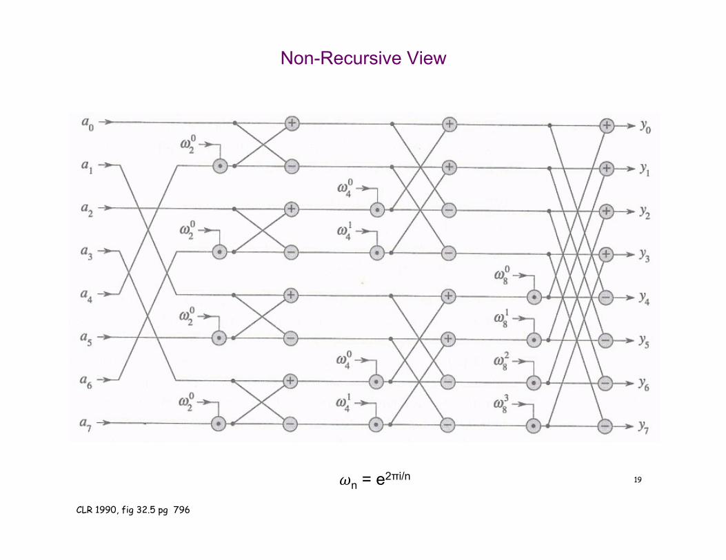
Non-Recursive View

19 𝜔n = e2πi/n

CLR 1990, fig 32.5 pg 796

20

Point-Value to Coefficient Representation: Inverse DFT

Goal. Given the values y0, ... , yn-1 of a degree n-1 polynomial at the n points ω0, ω1, …, ωn-1, find unique polynomial a0 + a1 x + ... + an-1 xn-1 that has given values at given points.

Inverse DFT

€

a0

a1

a2

a3

an−1

#

$

% % % % % % %

&

'

( ( ( ( ( ( (

=

1 1 1 1 11 ω1 ω2 ω3 ωn−1

1 ω2 ω4 ω6 ω2(n−1)

1 ω3 ω6 ω9 ω3(n−1)

1 ωn−1 ω2(n−1) ω3(n−1) ω(n−1)(n−1)

#

$

% % % % % % %

&

'

( ( ( ( ( ( (

−1

y0

y1y2

y3

yn−1

#

$

% % % % % % %

&

'

( ( ( ( ( ( (

Fourier matrix inverse (Fn)-1

21

Claim. Inverse of Fourier matrix is given by following formula. Consequence. To compute inverse FFT, apply same algorithm but use ω-1 = e -2π i / n as principal nth root of unity (and divide by n).

€

Gn =1n

1 1 1 1 11 ω−1 ω−2 ω−3 ω−(n−1)

1 ω−2 ω−4 ω−6 ω−2(n−1)

1 ω−3 ω−6 ω−9 ω−3(n−1)

1 ω−(n−1) ω−2(n−1) ω−3(n−1) ω−(n−1)(n−1)

$

%

& & & & & & &

'

(

) ) ) ) ) ) )

Inverse FFT

22

Inverse FFT: Proof of Correctness

Claim. Fn and Gn are inverses. Pf. Summation lemma. Let ω be a principal nth root of unity. Then Pf.   If k is a multiple of n then ωk = 1 ⇒ sums to n.   Each nth root of unity ωk is a root of xn - 1 =

(x - 1) (1 + x + x2 + ... + xn-1).   if ωk ≠ 1 we have: 1 + ωk + ωk(2) + . . . + ωk(n-1) = 0 ⇒ sums to 0. ▪

€

ω k j

j=0

n−1∑ =

n if k ≡ 0 mod n0 otherwise

& ' (

€

Fn Gn( ) k " k = 1n

ωk j ω− j " k

j=0

n−1∑ = 1

nω(k− " k ) j

j=0

n−1∑ =

1 if k = " k 0 otherwise& ' (

summation lemma

ω0 = 1

ω1

ω2 = i

ω3

ω4 = -1

ω5

ω6 = -i

ω7 n = 8

23

Inverse FFT: Algorithm

ifft(n, a0,a1,…,an-1) { if (n == 1) return a0 (e0,e1,…,en/2-1) ← FFT(n/2, a0,a2,a4,…,an-2) (d0,d1,…,dn/2-1) ← FFT(n/2, a1,a3,a5,…,an-1) for k = 0 to n/2 - 1 { ωk ← e-2πik/n yk+n/2 ← (ek + ωk dk) / n yk+n/2 ← (ek - ωk dk) / n } return (y0,y1,…,yn-1) }

24

Inverse FFT Summary

Theorem. Inverse FFT algorithm interpolates a degree n-1 polynomial given values at each of the nth roots of unity in O(n log n) steps.

assumes n is a power of 2

€

a0, a1,…, an-1

€

(ω0, y0 ), …, (ωn−1, yn−1)

O(n log n)

coefficient representation

O(n log n) point-value representation

25

Polynomial Multiplication

Theorem. Can multiply two degree n-1 polynomials in O(n log n) steps.

€

a0, a1,…, an-1b0, b1,…, bn-1

€

c0, c1,…, c2n-2

€

A(x0),…, A(x2n-1)B(x0 ),…, B(x2n-1)

€

C(x0),C(x1),…,C(x2n-1)O(n)

point-value multiplication

O(n log n) FFT inverse FFT O(n log n)

coefficient representation coefficient

representation

26

FFT in Practice

Fastest Fourier transform in the West. [Frigo and Johnson]   Optimized C library.   Features: DFT, DCT, real, complex, any size, any dimension.   Won 1999 Wilkinson Prize for Numerical Software.   Portable, competitive with vendor-tuned code.

Implementation details.   Instead of executing predetermined algorithm, it evaluates your

hardware and uses a special-purpose compiler to generate an optimized algorithm catered to "shape" of the problem.

  Core algorithm is nonrecursive version of Cooley-Tukey radix 2 FFT.   O(n log n), even for prime sizes.

Reference: http://www.fftw.org

27

Integer Multiplication

Integer multiplication. Given two n bit integers a = an-1 … a1a0 and b = bn-1 … b1b0, compute their product c = a × b.

Convolution algorithm.   Form two polynomials.   Note: a = A(2), b = B(2).   Compute C(x) = A(x) × B(x).   Evaluate C(2) = a × b.   Running time: O(n log n) complex arithmetic steps.

Theory. [Schönhage-Strassen 1971] O(n log n log log n) bit operations. [Fürer, 2007] (n log n ) 2O(log*n) [NB: log*n ≤ 5 for all practical purposes, but the big-O is nasty.] Practice. [GNU Multiple Precision Arithmetic Library] GMP proclaims to be "the fastest bignum library on the planet." It uses brute force, Karatsuba, and FFT, depending on the size of n.

€

A(x) = a0 + a1x + a2x2 ++ an−1x

n−1

€

B(x) = b0 +b1x +b2x2 ++ bn−1x

n−1

28

29

http

://w

ww

.sm

bc-c

omic

s.co

m/c

omic

s/20

1302

01.g

if