Divesting Power

Divesting Power∗

Giulio Federico† and Ángel L. López‡

December 15, 2009

Abstract

We study alternative market power mitigation measures in a model of the electricity mar-ket where a dominant producer faces a competitive fringe with the same cost structure. Wecharacterise the asset divestment by the dominant firm which achieves the greatest reduction inprices (taking the size of the divestment as given). The optimal divestment entails the sale ofassets which are price-setting post-divestment. A divestment of this type can be several timesmore effective in reducing prices than divestments of baseload (or low-cost) assets of the samesize. We also establish that Virtual Power Plant schemes are at best equivalent to baseloaddivestments in terms of their impact on consumer welfare, and cannot replicate the optimaldivestment.

JEL classification codes: D42, L13, L40, L94.Keywords: Divestments, Virtual Power Plants, contracts, market power, electricity, antitrust

remedies.

1 Introduction

Regulatory and antitrust proceedings often require the application of remedies, in order to mitigatethe market power of the affected parties or prevent a reduction in competition from a changein market structure. The appropriate remedy design often plays a critical role in ensuring thatcompetition remains effective in the presence of firms with market power. This paper studies theissue of optimal remedy design in a stylised model that is designed to capture the essential featuresof the wholesale electricity market. Our analysis focuses on the relative impact of different typesof asset divestments, and on the comparison between divestments and financial contracts (in theform of Virtual Power Plants (VPP)). Our framework and results are however applicable also to

∗The authors gratefully acknowledge financial support from the Spanish Ministry of Science and Technology underECO2008-05155/ECON. Ángel López also acknowledges financial support from the Juan de la Cierva Program.We are grateful to Ugur Akgün, Natalia Fabra, Kai-Uwe Kühn, Héctor Pérez, David Rahman, Pierre Régibeau,Patrick Rey, Flavia Roldán and Xavier Vives for their comments. We also received helpful suggestions from seminarparticipants at IESE (SP-SP), European Commission (DG-COMP), Bocconi (IEFE), and conference participants atEEM 2009 (Leuven), EEA 2009 (Barcelona) and EARIE 2009 (Ljubljana). The views expressed in this paper are theauthors’ own, and do not necessarily reflect those of the institutions to which they are affiliated.

†Public-Private Sector Research Center (IESE Business School), Barcelona GSE and Charles River Associates;[email protected]

‡Public-Private Sector Research Center (IESE Business School); [email protected]

1

industries which share some of the basic features of power generation (most notably, a homogenousfinal product and cost asymmetries between different assets).

In electricity generation markets, the divestment of actual and/or virtual capacity owned byproducers with market power is often employed as a remedy by competition authorities and sec-tor regulators to enhance competition. Outright plant divestments and VPP schemes have beenused across Europe in recent times, in the context of merger control proceedings, abuse of domi-nance investigations, and regulatory reviews of market power in electricity markets. Examples ofmergers or joint ventures in the electricity sector where divestments or VPPs have been requiredby the competition authorities include Gas Natural/Union Fenosa (2009), EDF/British Energy(2008), Gas Natural/Endesa (2006), GDF/Suez (2006), Nuon/Reliant (2003), ESB/Statoil (2002)and EDF/EnBW (2000).1 Alleged abuse of dominance cases where divestments of generation ca-pacity or VPPs have been implemented as a remedy include proceedings involving E.On (2008),RWE (2008) and Enel (2006). Divestments of power plants have also been used by regulatorsto mitigate market power of incumbent generators in the UK and Italy in the 1990s, whilst inSpain and Portugal regulatory contracts and more recently VPPs have been employed to make theelectricity market more competitive.

This paper analyses the competitive impact of divestments and of VPPs in a stylised model ofa wholesale electricity market where a dominant producer faces a competitive fringe with the samecost structure. The aim of the paper is two-fold: to study the differential impact of divestmentsdepending on the costs of the generation capacity that is sold by the dominant firm (and therebyidentify the divestment policy which achieves the largest reduction in prices); and to compare theeffectiveness of divestments of generation capacity with that of VPPs.

We find that the position of the divested capacity on the marginal cost curve of the dominantfirm has a strong effect on the impact that a divestment has on market prices. For sufficiently largedivestments, the divestment policy which achieves the greatest reduction in prices (which we defineas the “optimal” divestment) is the one which divests marginal plants, whose range of costs encom-passes the post-divestment equilibrium price (at a given demand level). The optimal divestmentincludes capacity whose highest cost lies below the pre-divestment price (i.e. capacity that is beingstrategically withheld from the market by the dominant firm), but above the competitive price (i.e.whose costs are not ‘too’ low). In particular, unless the divestment is relatively large (i.e. strictlylarger than the output withheld by the dominant firm relative to the competitive equilibrium), thedivestment should not include the cheapest capacity withheld from the market, and should insteadinclude more expensive capacity (as long as it is not too expensive). Only if the divestment isabove a certain size threshold, it should then optimally include the lowest-cost capacity withheldby the dominant firm relative to the competitive benchmark. In this case the optimal divestmentalso achieves the competitive price.

We find that the optimal divestment induces the dominant firm to price on the flatter segment ofits residual demand curve. Depending on the size of the divestment, the most effective divestment

1Divestments of generation capacity were also implemented in the British market in the context of two mergersinvolving the incumbent generators and retail suppliers during the 1990s.

2

can reduce prices several times more than the divestment of baseload plants (i.e. capacity used bythe dominant firm in the pre-divestment equilibrium). We also find that the optimal divestmentalways increases total welfare (or efficiency), whilst this is not the case for all types of divestments.Our results on divestments have implications for the assessment of the impact of independent entry,showing that the entry of marginal plants can be significantly more effective in reducing prices thanthe entry of baseload plants.

The paper compares the optimal divestment policy to VPP arrangements. We abstract in ourmodelling from some of the potential advantages of VPPs, including the fact that they may be easierand faster to implement than plant divestments, and can be reversed once competitive conditionsimprove. We also do not model some of the shortcomings of VPPs which have been identified indynamic settings (e.g. the fact that they may not mitigate market power effectively if VPP auctionsare repeated over time, thereby potentially giving incentives to producers with market power toincrease spot prices to affect future VPP revenues).

We model VPPs as a set of several call options on the output of the dominant firm with differentexercise prices. We establish that VPPs are always weakly less effective than plant divestments inreducing prices and they can at best replicate the impact of a baseload divestment (if the strikeprices are set sufficiently low, implying that the VPP works like a forward contract). This resultimplies that setting the strike prices of a VPP so as to mimic the variable costs of marginal plantsdoes not increase the effectiveness of the remedy. In particular, it does not ensure that the sale ofvirtual plants will be as effective as the corresponding divestment of generating capacity in reducingprices.

There is a relatively limited literature on the impact of divestments and VPPs on market powerin electricity generation markets, and on their relative effectiveness. Green (1996) is a relativelyearly contribution which considers the impact of divestments in a model of supply-function equilib-rium. He focuses on divestments that apply uniformly to the entire portfolio of the larger incumbentgenerators, which can therefore be modelled by simply changing the slope of the respective costcurves. This approach generates analytical convenient results, but cannot be used to analyse di-vestments of assets that are located at different positions on the cost curve of a dominant generator(which is the main focus of our paper).

A significant part of the related academic research to date has focused on the impact of forwardcontracts on market power. This literature is relevant to VPPs since forward contracts can beinterpreted as call options which are exercised by the option holder independently of the spot price(i.e. the options are always “in the money”). This strand of the literature was started by thecontribution by Allaz and Vila (1993), which established that forward contracts can significantlyincrease competition in spot markets in a Cournot duopoly model. Newbery (1998), Green (1999),and Bushnell (2007) extend some of the results established by Allaz and Vila to competition insupply functions and Cournot competition with multiple firms, in the specific context of electricitymarkets.

More recently some papers have noted that the pro-competitive impact of forward contractsin electricity markets may be mitigated in the presence of repeated interaction with or withoutasymmetric information on the costs of the dominant firms (see Schultz, 2007, and Zhang and

3

Zwart, 2006 respectively), or if contracts are not assigned to the largest firms in the market, in amodel with discrete bidding functions (Fabra and de Frutos, 2008). Our paper shows that evenin the absence of these circumstances, contracts and/or VPPs are inferior to divestments as aninstrument to increase competition in electricity markets.

Willems (2006) is more closely related to our paper. Willems compares the effectiveness of“financial” and “physical” VPPs, where the latter are defined as options for capacity that aredirectly bid in the market by the option holder (whilst financial VPPs are simply call options whichare settled once the spot market clears). He finds that the market is more competitive with physicalrather than financial options, due to the assumed impact of physical options on the conjecturesmade by strategic players. The effect identified by Willems is not present in our framework, sincephysical and financial options are equivalent in the absence of strategic interaction (which is thecase for the residual monopoly setting with a competitive fringe that we adopt). Nonetheless wefind that − even in a residual monopoly framework − divestments and VPPs can have a verydifferent impact on market prices, due to the fact that divestments have different properties thanphysical options (as modelled by Willems) and can be significantly more pro-competitive thanoption contracts.

More generally, the results presented in this paper are related to some of the points noted byArmington et al. (2006) and Wolak and McRae (2008). These two articles discuss in qualitativeterms how divestments of generation capacity can be utilised to remedy the expected impact of amerger on prices, using the specific example of the proposed Exelon/PSEG merger in the US in2006. The remedies imposed by the US Department of Justice in that merger focused on divesting‘ability’ assets, whose costs were close to the market clearing price, implying that the merged entityfaced a low opportunity cost of withholding them from the market. By divesting these plants, thecompetition authority sought to reduce the ability and incentives of the merging parties to increaseprices. The results presented in our paper formalise and extend this intuition, identifying exactlywhich ability assets should be divested to maximise the pro-competitive impact of the remedy (fora given level of demand). Our results also provide formal support to the relatively commonly-heldview in the literature and decision practice on electricity markets that ownership of price-settingassets confers greater market power than ownership of baseload plants, even though both types ofassets contribute to the presence of market power (for a discussion see Newbery, 2005, and Federicoet al. 2008; see also OECD, 2005 for some related results).

The structure of the remainder of this paper is as follows. Section 2 describes the set-up ofour model, including a characterisation of the residual monopoly (or pre-divestment) equilibrium.Section 3 solves the case of divestments of intermediate size (which we treat as our benchmarkdivestment scenario). Section 4 presents our results for VPPs, comparing them to those obtainedfor intermediate divestments. Section 5 extends our core results to the cases of small and largedivestments, whilst Section 6 concludes.

4

2 Model set-up

We model a market with a dominant electricity firm facing a competitive fringe that offers all of itsoutput at cost.2 We also assume for simplicity that pre-divestment the dominant firm and the fringehave the same linear and increasing marginal cost function, with slope γ. The marginal cost functioncan be interpreted as the aggregation of production from several atomistic generation plants withdifferent marginal costs, stacked in ‘merit order’, from the cheapest to the most expensive. Wedefine marginal costs for each firm i as ci and output as qi. We also adopt subscript d for thedominant firm and f for the fringe. Our set-up implies that ci = γqi for i = d, f .

We also assume that total demand is perfectly price inelastic and takes a value of µ. We assumea constant willingness to pay for consumers that lies above the pre-divestment equilibrium price.This ensures that total and consumer surplus are finite. The assumption of inelastic demand alsoimplies that consumer welfare decreases monotonically with the market price, and that total welfareincreases if total production costs decrease.

2.1 Pre-divestment equilibrium

For a given price p, the competitive fringe always produce at its marginal cost: p = cf = γqf , whereqf = µ− qd, implying that p = γ(µ− qd).

The dominant firm solves maxp pqd−∫cddq, which is equivalent to solving maxqd γ(µ−qd)qd−

(γ/2)(qd)2. The first-order condition yields:3

q∗d =µ

3; and p∗ =

2

3γµ

where the latter defines the residual monopoly (or pre-divestment) price level.In the pre-divestment equilibrium the dominant firm therefore serves a third of demand, rather

than half of demand as it would in a competitive equilibrium. The quantity between µ2 and µ

3 iswithheld from the market, forcing more expensive generation units owned by the fringe to produce,thereby raising prices and lowering both consumer and total welfare. Note that the competitiveprice (i.e. the price which would result if all production plants in the market were offered at theirmarginal cost) is given by pc = 1

2γµ.

2Whilst this set-up is stylised, it is also a reasonable representation of the competitive structure of a number ofEuropean power markets, including Belgium, France, Ireland, Italy, and Portugal. The results that we present beloware also directly applicable to the competitive residual demand framework proposed by Gilbert and Newbery (2008)for the evaluation of mergers in the electricity sector. Our results can also be applied to oligopoly models whichassume that firms compete with discrete bids. In these models in any given pure-strategy equilibrium only one firmexercises market power and other firms behave as if they offered of all their output at cost (see Fabra and de Frutos,2008). This implies that as long as a given equilibrium continues to exist after the application of a divestment/VPPto the price-setting firm, such equilibrium can be characterised using the model of a dominant firm with a competitivefringe.

3The second-order conditions are satisfied throughout the analysis.

5

2.2 Definition of divestment

We model divestments of generation units that are located contiguously on the marginal costfunction of the dominant firm. The maximum output (or capacity) that can be produced by thedivested units is defined as δ. This parameter describes the ‘size’ of the divestment. We treat δ asan exogenous parameter in our model. This parameter can interpreted as the outcome of a bargainbetween a regulator that seeks to mitigate market power and other groups which oppose suchintervention. In the context of a specific antitrust procedure, the size of the divestment can also bethought of as the smallest intervention required to eliminate the price increase that is associatedwith a competition concern (e.g. a merger, or an abuse of dominance).

We define the marginal cost of the most expensive divested unit as c. This uniquely defines the‘position’ of the divestment on the cost curve of the dominant firm. The marginal cost of the leastexpensive divested unit is therefore given by c = c− γδ . For notational purposes we also define q′

as follows: q′ = cγ.4

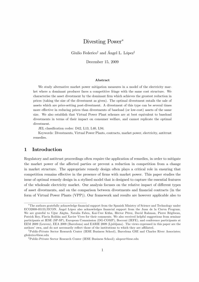
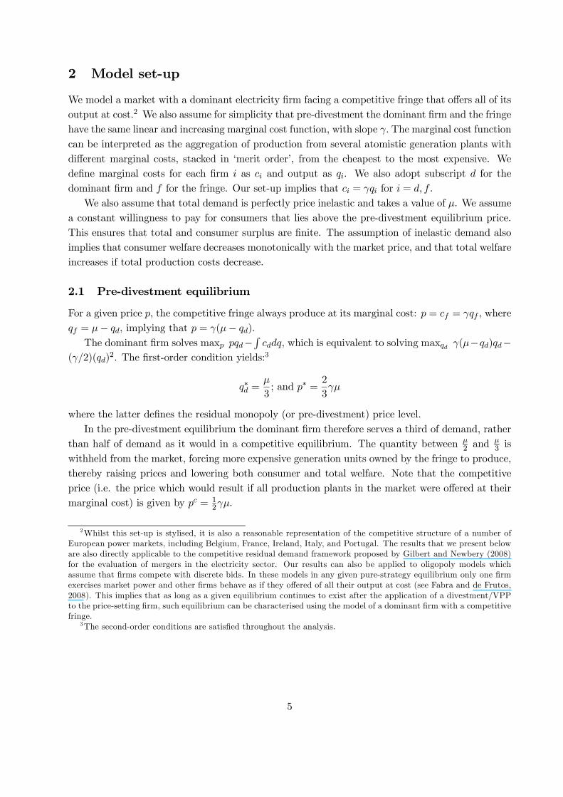
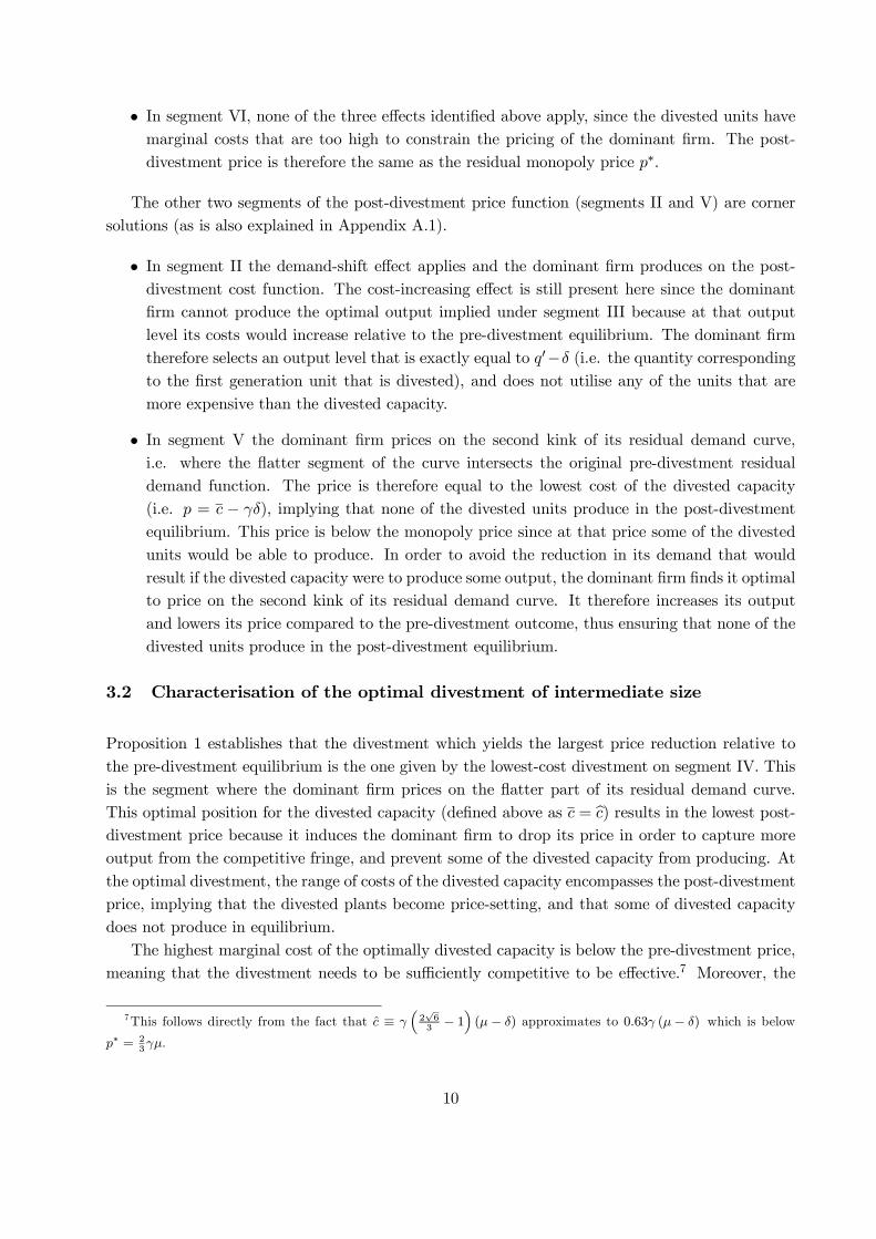
Divested generation units are assigned to the competitive fringe and are therefore offered tothe market at cost in the post-divestment equilibrium.5 Relative to the pre-divestment set-up,post-divestment the marginal cost curve of the dominant firm shifts upwards for cd > c− γδ andits residual demand curve is lower for p > c−γδ . It is also flatter than the pre-divestment residualdemand function for p ∈ (c − γδ, c), whilst for p ≥ c it has the same slope as the pre-divestmentresidual demand function, but it is displaced downwards by the size of the divestment δ. Theimpact of a divestment on the marginal cost and residual demand functions of the dominant firmis illustrated in Figure 1.

The rest of this paper focuses on the impact on market prices (and therefore consumer welfare)of divestments of size δ, depending on their location on the cost curve of the dominant firm (givenby c). We primarily concentrate on consumer welfare rather than total welfare in our assessmentof divestments given that competition authorities and sector regulators are typically concernedwith policies which benefit consumers. We however also comment on the welfare implications ofalternative divestment policies.

We rely on this set-up to model also the impact on prices of VPPs. VPPs are analysed as calloptions that are structured so as to mimic a given plant divestment. That is, we consider a bundleof call options of total size δ with contiguous strike prices ranging from c to c−γδ. This modellingassumption (which is without loss of generality) is set out in more detail in Section 4 below.

4This variable defines the total output that the dominant firm would produce in the pre-divestment set-up if theunit with marginal cost c were its last (or marginal) unit to be offered to the market and accepted for production.It can also be interpreted as a quantity index along the cost curve of the dominant firm, which also describes theposition of the divested segment (in terms of quantities rather than costs).

5We assume that the divested capacity is transferred through a competitive auction process, which determinesa lump-sum payment from the fringe to the dominant firm in exchange for the production capacity. The sameassumption holds for the transfer of the VPP contract.

6

Slope = -

Slope = -

µ'q

γ

2

γ

dqγ

γµ

( )δµγ −

c

γδ−c

δ−'q

Divested capacity

( )δγ +dq

Pre-divestment

residual demand

Pre-divestment

marginal cost

dq

p

δµ−

Slope = -

Slope = -

µ'q

γ

2

γ

dqγ

γµ

( )δµγ −

c

γδ−c

δ−'q

Divested capacity

( )δγ +dq

Pre-divestment

residual demand

Pre-divestment

marginal cost

dq

p

δµ−

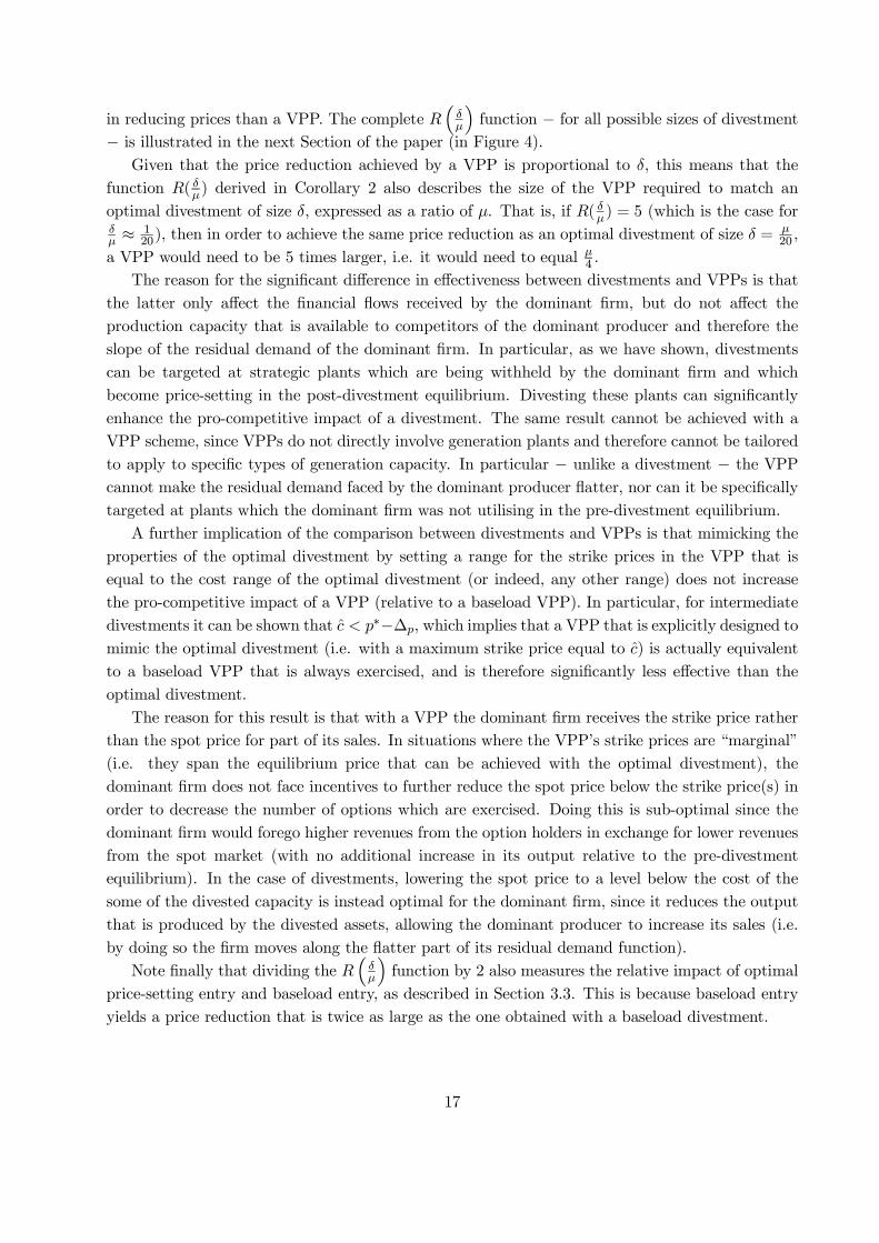
Figure 1: Description of the model set-up and of the impact of a divestment.

3 Divestments of intermediate size

In this section of the paper we model divestments of intermediate size, defined as cases where δ,expressed as a ratio of total demand µ (i.e. δ

µ), lies between two threshold values: 1− 125√6≈ 0.02

and 1 − 2√6≈ 0.18. This is a relative wide range for the divestment, which we feel captures

most realistic divestment scenarios.6 Note that the upper bound of this range strictly exceeds theamount of output withheld by the dominant firm in the pre-divestment equilibrium relative to thecompetitive benchmark (i.e. δ

µ =16). In Section 5 below we extend our results to cases with smaller

and larger divestments.

3.1 Prices with divestments of intermediate size

The following Proposition describes the post-divestment price function for divestments of inter-mediate size, as a function of the position of the divested plants. As we show, a unique optimal

6For example, in the case of the Spanish wholesale electricity market which had average demand in 2007 ofapproximately 30GW, the range for the divestments that we consider here is between 0.6GW and 5.5GW (evaluatedat average demand). As a comparison, the total size of the VPP imposed on the two largest producers (Endesaand Iberdrola) in 2008 and 2009 reached roughly 2.5GW, and that of the plant divestments ordered by the Spanishgovernment in two recent domestic mergers (the proposed merger between Gas Natural and Endesa, and the approvedmerger between Gas Natural and Union Fenosa) were of 4.2GW and 2 GW respectively (see Federico et al. 2008).

Another example of divestments is provided by the merger between EDF and British Energy in the British market,where the European Commission imposed a divestment of 2.8GW of generation capacity in December 2008. This isequivalent to roughly 0.07 of average electricity demand in Great Britain, which is also within the range of intermediatedivestments that we consider.

7

divestment can be identified. The optimal divestment is defined as the one that leads to the lowestprice (and therefore the highest level of consumer welfare) in the post-divestment equilibrium.

Proposition 1 (Intermediate divestments) The post-divestment price function depends on the

position of the plant divestment (denoted by c). For divestments of intermediate size, this function

(defined as p(c)) has 6 distinct segments:

Segment Price Range of c

I (baseload) p∗ −∆p γδ ≤ c < p∗

2 +∆p

II γµ− c p∗

2 +∆p ≤ c <p∗

2 + 2∆p

III p∗ − 2∆p p∗

2 + 2∆p ≤ c < γ(2√63 − 1

)(µ− δ)

IV 38(γ(µ− δ) + c) γ

(2√63 − 1

)(µ− δ) ≤ c < γ(35µ+ δ)

V c− γδ γ(35µ+ δ) ≤ c < p∗ + 3∆pVI p∗ c ≥ p∗ + 3∆p

,

where ∆p ≡ γδ3 .

The optimal divestment is given by setting c = c ≡ γ(2√63 − 1

)(µ− δ) , which defines the lower

bound of segment IV of the post-divestment price function. The optimal divestment achieves the

competitive price pc at the upper end of the range for the size of the divestment considered in this

Proposition (i.e. if δµ = 1− 2√6). Otherwise it yields a price that is between pc and p∗.

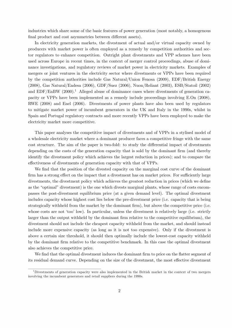
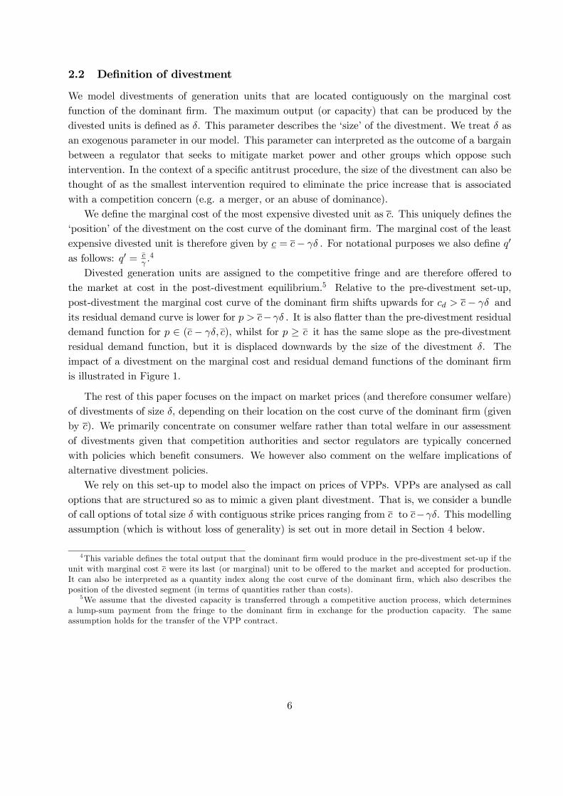
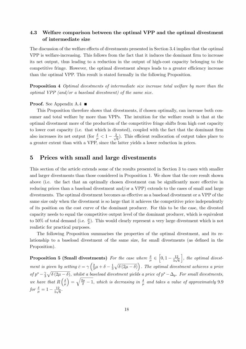
Proof. See Appendix A.1.The post-divestment price function is shown in Figure 2, as a function of the position of the

divestment c. As the figure illustrates this function lies below the pre-divestment price p∗ fordivestments that are sufficiently competitive, which is the case for c sufficiently low (i.e. c <

p∗ + 3∆p).The six segments in the post-divestment price function can be understood by reference to the

impact of a divestment on the cost and demand of the dominant firm. As we noted above, adivestment increases the cost function of the dominant firm above a given marginal cost level(i.e. for cd > c − γδ). This can be defined as a cost-increasing effect. This effect is relevantto equilibrium pricing for divestments of production capacity whose marginal cost is sufficientlylow (implying that the dominant firm is utilising at least part of the divested capacity in the pre-divestment equilibrium). Note that the presence of the cost-increasing effect tends to reduce thepro-competitive impact of a divestment because it induces the dominant firm to set higher prices,ceteris paribus, since its costs are higher.

A divestment also changes the residual demand curve of the dominant firm, introducing a flattersegment, and also displacing it downwards by the size of the divestment δ for sufficiently high pricelevels (i.e. p > c), as it is shown in Figure 1. We term the first demand effect a demand-slopeeffect, whilst the second demand effect is termed a demand-shift effect.

The four segments of the post-divestment price function where interior equilibria exist (theseare segments I, III, IV and VI − see Appendix A.1) display different combinations of these three

8

*p

pp ∆−*

pp ∆− 2*

)(13

62δµγ −

−

+δµγ

5

3p

p ∆+ 3* c

p

I II III IV V VI

( )cp

p

p∆+

2

*

p

p∆+ 2

2

*

*p

pp ∆−*

pp ∆− 2*

)(13

62δµγ −

−

+δµγ

5

3p

p ∆+ 3* c

p

I II III IV V VI

( )cp

p

p∆+

2

*

p

p∆+ 2

2

*

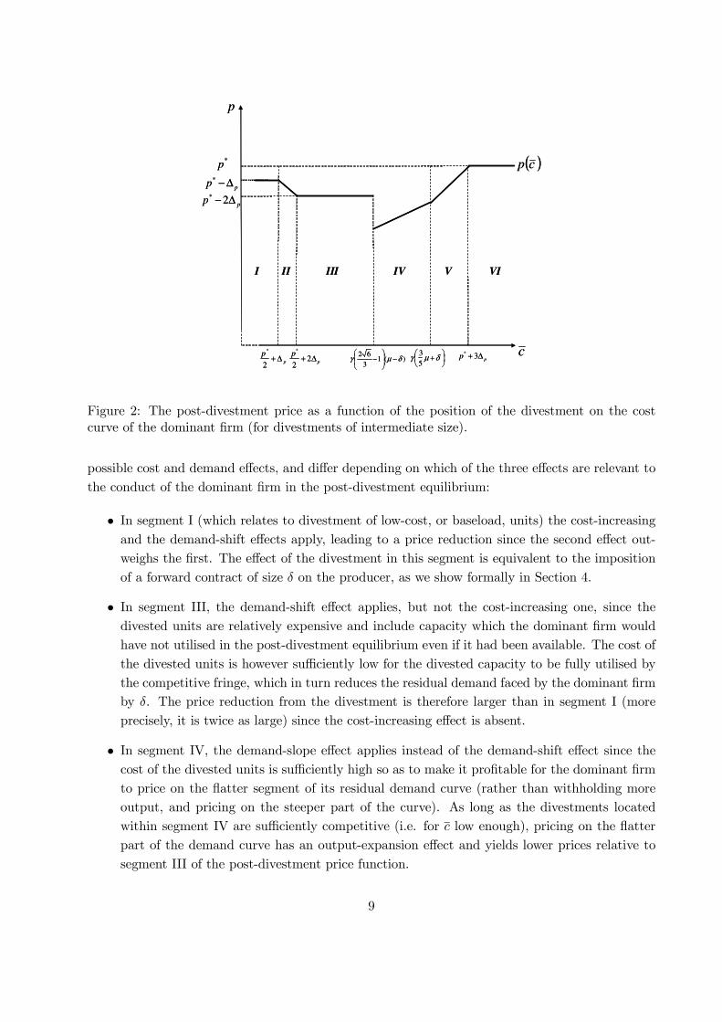
Figure 2: The post-divestment price as a function of the position of the divestment on the costcurve of the dominant firm (for divestments of intermediate size).

possible cost and demand effects, and differ depending on which of the three effects are relevant tothe conduct of the dominant firm in the post-divestment equilibrium:

• In segment I (which relates to divestment of low-cost, or baseload, units) the cost-increasingand the demand-shift effects apply, leading to a price reduction since the second effect out-weighs the first. The effect of the divestment in this segment is equivalent to the impositionof a forward contract of size δ on the producer, as we show formally in Section 4.

• In segment III, the demand-shift effect applies, but not the cost-increasing one, since thedivested units are relatively expensive and include capacity which the dominant firm wouldhave not utilised in the post-divestment equilibrium even if it had been available. The cost ofthe divested units is however sufficiently low for the divested capacity to be fully utilised bythe competitive fringe, which in turn reduces the residual demand faced by the dominant firmby δ. The price reduction from the divestment is therefore larger than in segment I (moreprecisely, it is twice as large) since the cost-increasing effect is absent.

• In segment IV, the demand-slope effect applies instead of the demand-shift effect since thecost of the divested units is sufficiently high so as to make it profitable for the dominant firmto price on the flatter segment of its residual demand curve (rather than withholding moreoutput, and pricing on the steeper part of the curve). As long as the divestments locatedwithin segment IV are sufficiently competitive (i.e. for c low enough), pricing on the flatterpart of the demand curve has an output-expansion effect and yields lower prices relative tosegment III of the post-divestment price function.

9

• In segment VI, none of the three effects identified above apply, since the divested units havemarginal costs that are too high to constrain the pricing of the dominant firm. The post-divestment price is therefore the same as the residual monopoly price p∗.

The other two segments of the post-divestment price function (segments II and V) are cornersolutions (as is also explained in Appendix A.1).

• In segment II the demand-shift effect applies and the dominant firm produces on the post-divestment cost function. The cost-increasing effect is still present here since the dominantfirm cannot produce the optimal output implied under segment III because at that outputlevel its costs would increase relative to the pre-divestment equilibrium. The dominant firmtherefore selects an output level that is exactly equal to q′−δ (i.e. the quantity correspondingto the first generation unit that is divested), and does not utilise any of the units that aremore expensive than the divested capacity.

• In segment V the dominant firm prices on the second kink of its residual demand curve,i.e. where the flatter segment of the curve intersects the original pre-divestment residualdemand function. The price is therefore equal to the lowest cost of the divested capacity(i.e. p = c − γδ), implying that none of the divested units produce in the post-divestmentequilibrium. This price is below the monopoly price since at that price some of the divestedunits would be able to produce. In order to avoid the reduction in its demand that wouldresult if the divested capacity were to produce some output, the dominant firm finds it optimalto price on the second kink of its residual demand curve. It therefore increases its outputand lowers its price compared to the pre-divestment outcome, thus ensuring that none of thedivested units produce in the post-divestment equilibrium.

3.2 Characterisation of the optimal divestment of intermediate size

Proposition 1 establishes that the divestment which yields the largest price reduction relative tothe pre-divestment equilibrium is the one given by the lowest-cost divestment on segment IV. Thisis the segment where the dominant firm prices on the flatter part of its residual demand curve.This optimal position for the divested capacity (defined above as c = c) results in the lowest post-divestment price because it induces the dominant firm to drop its price in order to capture moreoutput from the competitive fringe, and prevent some of the divested capacity from producing. Atthe optimal divestment, the range of costs of the divested capacity encompasses the post-divestmentprice, implying that the divested plants become price-setting, and that some of divested capacitydoes not produce in equilibrium.

The highest marginal cost of the optimally divested capacity is below the pre-divestment price,meaning that the divestment needs to be sufficiently competitive to be effective.7 Moreover, the

7This follows directly from the fact that c ≡ γ(2√6

3− 1

)(µ− δ) approximates to 0.63γ (µ− δ) which is below

p∗ = 23γµ.

10

cost range of the optimal divestment lies above both the costs of the cheapest units withheld bythe dominant firm in the pre—divestment equilibrium, and the competitive price pc.8 If one thinksas the cheapest withheld units as the marginal, or price-setting units, of the dominant firm in thepre-divestment equilibrium (e.g. as would be the case if the dominant producer was constrainedto offer a linear supply function for its output), this condition implies that the optimal divestmentneeds to include units which are bid above the pre-divestment price (i.e. they are outside thecompetitive margin), but which become price-setting post-divestment when they are owned by thecompetitive fringe.

The figure presented in Appendix A.7 provides an illustration of the position of the optimaldivestment for the case of δµ =

120 .

The following Corollary summarises the main characteristics of the optimal divestment.

Corollary 1 (Characteristics of the optimal divestment) For intermediate values of δ, to

achieve an optimal divestment the highest cost of the divested capacity needs to be located between the

competitive and the pre-divestment price, that is: c ∈ (pc, p∗). The costs of the optimal divestmentalso need to encompass the post-divestment price, that is: p (c) ∈ [c− γδ, c).

Marginally cheaper divestments than the optimal divestment have a lower pro-competitive effect(even if they do not include baseload plants, as it is the case in segment III of the post-divestmentprice function). This is due to the fact that the price which the dominant firm would need to acceptto exclude some of the divested capacity from the market is too low. In this case the dominantfirm finds it optimal to set a higher price and accept a larger reduction of its residual demand.Marginally more expensive divestments than the optimal divestment are also less effective, sincethey put less competitive pressure on the dominant firm (i.e. a lower price reduction is required toprevent at least some of the divested capacity from producing).

3.3 Implications for the impact of entry on prices

The price results obtained above also have some implications for the impact of entry by independentfirms on market prices.9 To see this, assume for simplicity that new capacity of size δ belonging tothe competitive fringe can enter the market, with marginal costs ranging from c to c − γδ, alonga linear cost function of slope γ. Entry of this type shifts the residual demand function of thedominant firm in the same way as a divestment but does not affect its cost curve. Its impact onprices is therefore the same as that obtained with a divestment, as long as the dominant firm priceson its pre-divestment cost function (i.e. its costs do not increase relative to the pre-divestmentequilibrium). This is the case in segments III to VI of the post-divestment price function.

Proposition 1 therefore effectively establishes that entry of low-cost (or baseload plants) ofcapacity δ leads to a price reduction equal to the one given in segment III, since in this segment ofthe post-divestment price function the residual demand faced by the dominant firm shifts by δ and

8The former follows from the fact that c ≥ γ(µ3 + δ) (which is shown in Appendix A.1). The latter derives from

the fact that c > γµ

2, which is the case for δ

µ< 4

√6−9

4√6−6 (which is satisfied in the case of intermediate divestments).

9This discussion assumes that entry decisions and the cost of new capacity are exogenous.

11

the dominant firm does not price on the flatter part of its residual demand. Entry can thereforebe defined as baseload in our set-up as long as the highest cost of the new capacity entering themarket is strictly below c. However, entry can also replicate the impact of the optimal divestment ifthe highest cost of new capacity of size δ equals exactly c.10 Proposition 1 therefore indicates thatmarginal (or price-setting) entry is more effective than baseload entry in constraining market prices,assuming the cost of the new capacity is determined by the same cost function as the dominantfirm.

3.4 Welfare analysis of intermediate divestments

Our assumption of perfectly inelastic demand implies that divestments increase total welfare (orefficiency) if they reduce the total costs of producing the fixed level of output µ. A divestmentaffects total costs by leading to three distinct output effects: (i) a reduction in the output ofhigh-cost capacity owned by the fringe (which takes place as long as the divestment leads to areduction in prices); (ii) an increase in the output by the divested units (which occurs as long asthe divestment is price-reducing and the dominant firm is not using all of the divested capacityin the pre-divestment equilibrium); and (iii) a change in the net output of the dominant firm (i.e.output net of any part of the divested capacity which was being utilised by the dominant firm in thepre-divestment equilibrium). These three output effects necessarily sum to 0, given the assumptionof inelastic aggregate demand.

Using the case of the optimal divestment to illustrate the impact of these three output effects,the change in welfare from the optimal divestment can therefore be expressed as follows:11

∆W (c) =

23µ∫

p(c)γ

γxdx

︸ ︷︷ ︸cost saving

competitive fringe

−

p(c)γ∫

q−δ

γxdx

︸ ︷︷ ︸additional costdivested units

−

µ+q−δ4∫

µ3

γxdx

︸ ︷︷ ︸

.

additional costdominant firm

Divestments are welfare-increasing as long as they do not induce the dominant firm to reduceits net output (as defined above). This follows from the assumption of increasing marginal costs,which in turns implies that both the output increase by the divested capacity in the post-divestmentequilibrium and any net output increase by the dominant firm have lower marginal costs than thecapacity of the competitive fringe that no longer produces post-divestment.

The following Proposition summarises the welfare effects of divestments of intermediate size.

10Note of course that entry of capacity with highest cost equal to c will not be all used in the market for a givendemand level µ. If demand is fixed at µ therefore it will not be profitable to build such capacity. If demand is variablehowever, then it may be profitable to invest capacity that is price-setting at low or medium demand levels, and thatis infra-marginal during high demand levels.

11Recall from Proposition 1 that c = γ(2√6

3 − 1)(µ− δ) and that q = c

γ. The proof of Proposition 1 also

establishes that µ+q−δ4 is the output of the dominant firm in the case of the optimal divestment.

12

Proposition 2 (Welfare) Divestments of intermediate size are welfare-increasing for all the ranges

of c given in Proposition 1, except for segment III, where c ∈[p∗

2 + 2∆p, γ(2√63 − 1

)(µ− δ)

). In

this range of the costs of the divested units, divestments can reduce welfare for sufficiently small

divestments, i.e. for δµ ∈

(1− 12

5√6, 6√6−14

6√6−7

).

Proof. See Appendix A.2.The result given in Proposition 2 follows from the fact that - for intermediate divestments

- the net output of the dominant firm falls only in the range of costs which applies to segmentIII of the post-divestment price function (as defined in Proposition 1). For this range of costs,the divestment affects capacity that the dominant firm was not utilising pre-divestment, and thedominant firm reduces its output due to a reduction in its residual demand. As it is shown in theproof of Proposition 1, the net output of the dominant firm falls by δ

3 in this case. This creates aproductive inefficiency which can lead to an overall reduction in total welfare, for sufficiently smalldivestments, as Proposition 2 establishes.

The dominant firm’s net output increases for intermediate divestments located other than inthe cost range which applies to segment III of the post-divestment price function. As a result, totalproduction costs are necessarily lower post-divestment in these other cases. Note that Proposition2 also establishes that the optimal divestment from a consumer welfare perspective always increasestotal welfare as well, compared to the pre-divestment outcome.

4 Virtual Power Plants

In this section of the article we describe the impact of financial contracts (modelled as VPPs) onequilibrium prices, in the same model of a dominant firm facing a competitive fringe consideredabove for the case of divestments. VPPs are typically structured as call options that are imposedon a producer for a certain part of its generation output. The option holders have a right toacquire electricity from the generator at a strike (or exercise) price ps, and can re-sell this outputin the spot market to obtain the market price p.12 The option will therefore be exercised wheneverp > ps. We assume that both the volumes associated with these options and the strike prices areset exogenously by a regulator for market power mitigation purposes. In what follows we analysethe impact of VPPs from a static perspective, and abstract from some of potential institutionaladvantages associated with VPPs (as discussed in the Introduction).

For analytical convenience, so as to obtain results which are directly comparable to those derivedabove in relation to divestments, we assume that the VPP scheme entails the sale of a group ofinfinitesimally small call options each with a different strike price.13 The sum of the volumesassociated with the aggregate set of options equals δ. The strike prices associated with each optionare defined along an increasing and continuous linear function that has the same slope (γ) as the

12We assume that multiple players hold the options and do not have any market power when exercising theiroptions.

13This set-up is similar to that employed by Willems (2006) to describe the impact of VPPs.

13

marginal cost function of the dominant firm.14 The VPP scheme that we model is therefore designedto mimic a physical plant divestment of size δ, from a firm with a linear and increasing marginalcost function with slope γ. As in the case of divestments, the highest strike price associated witha VPP can also be expressed as c, implying that the lowest strike price is given by c − γδ. Thisallows for a direct comparison of the relative impact of a VPP and of a divestment that have thesame position on the cost curve of the dominant firm, as measured by c. The restriction on theshape of the VPP does not affect the results on the nature of the optimal VPP (i.e. the VPP whichleads to the largest reduction in spot prices). In particular, as we show below, the effectiveness ofa VPP is maximised by choosing a set of strike prices that are such that the option is exercised inits entirety. This result is independent of the slope of the strike price function that is assumed, andis also obtained with a constant strike price (i.e. setting strike prices according to more complexformulae does not affect this result).

4.1 Prices with VPPs

The following Proposition describes the impact of a VPP on prices, depending on the strike pricesassociated with the scheme.

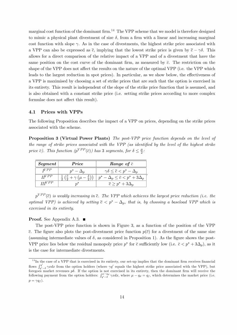
Proposition 3 (Virtual Power Plants) The post-VPP price function depends on the level of

the range of strike prices associated with the VPP (as identified by the level of the highest strike

price c). This function (pV PP (c)) has 3 segments, for δ ≤ µ2 :

Segment Price Range of c

IV PP p∗ −∆p γδ ≤ c < p∗ −∆pIIV PP 1

2

(c2 + γ

(µ− δ

2

))p∗ −∆p ≤ c < p∗ + 3∆p

IIIV PP p∗ c ≥ p∗ + 3∆p

,

pV PP (c) is weakly increasing in c. The VPP which achieves the largest price reduction (i.e. the

optimal VPP) is achieved by setting c < p∗ − ∆p, that is, by choosing a baseload VPP which isexercised in its entirety.

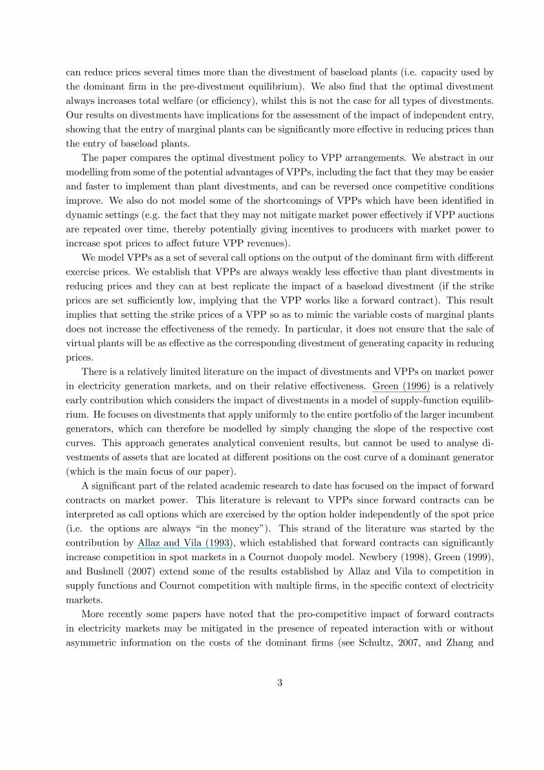
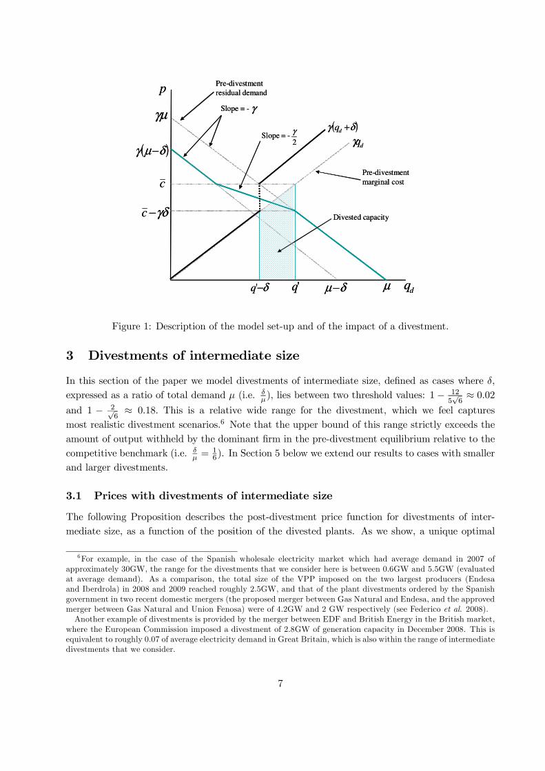
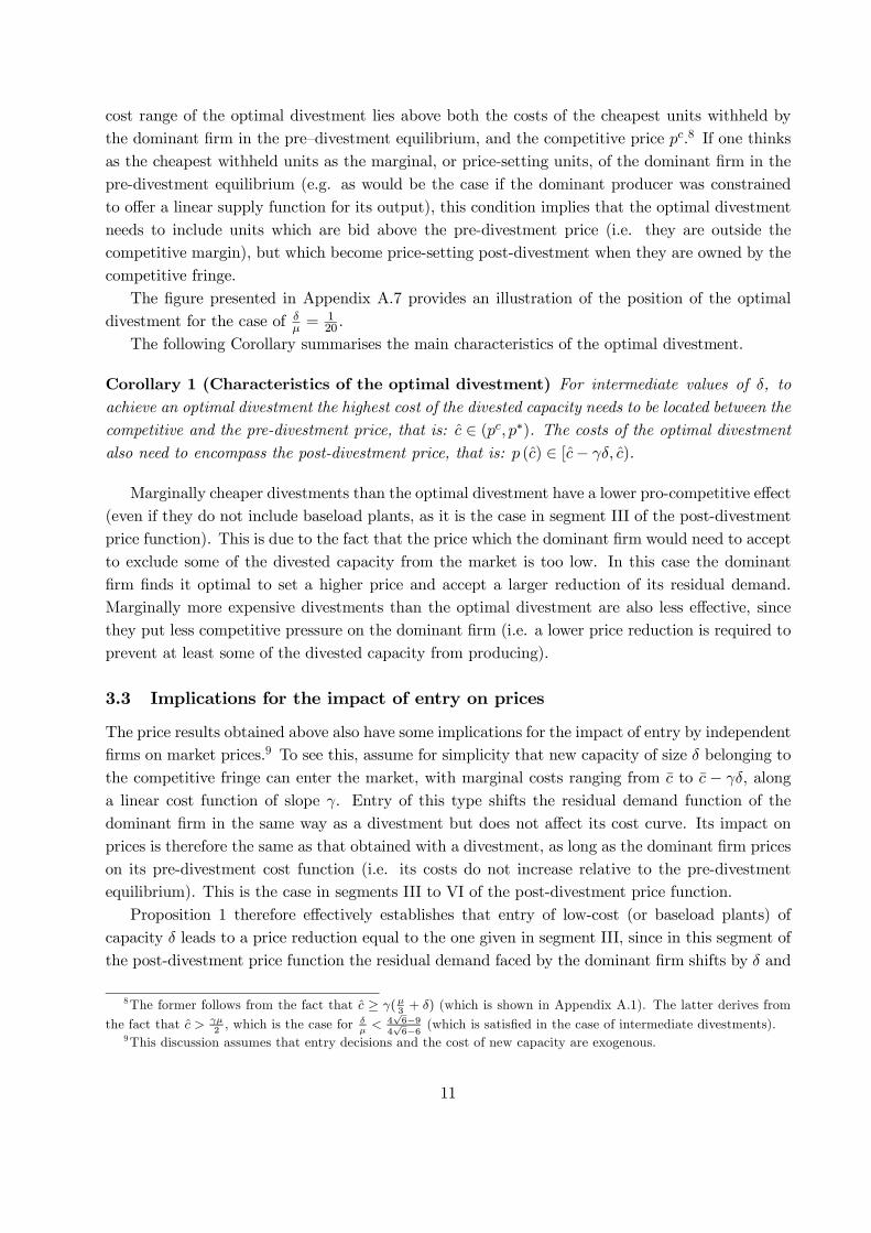
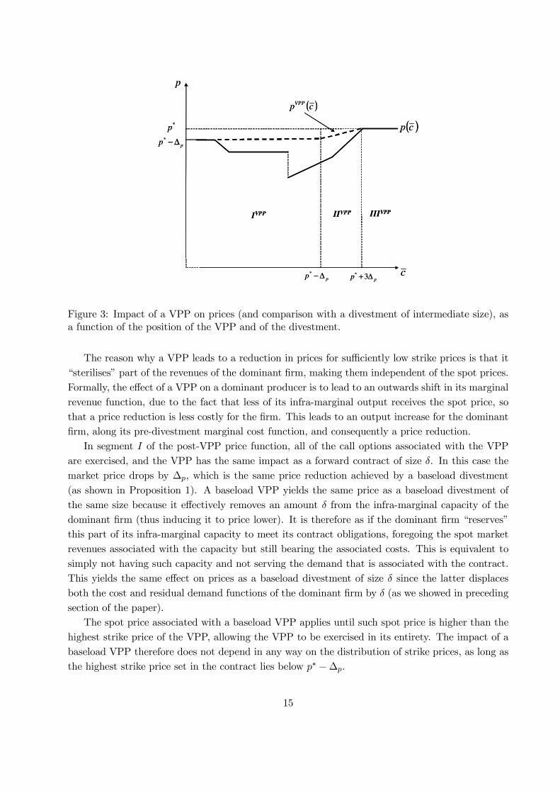
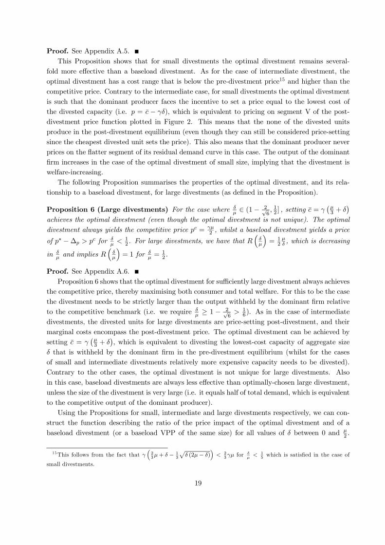
Proof. See Appendix A.3.The post-VPP price function is shown in Figure 3, as a function of the position of the VPP

c. The figure also plots the post-divestment price function p(c) for a divestment of the same size(assuming intermediate values of δ, as considered in Proposition 1). As the figure shows the post-VPP price lies below the residual monopoly price p∗ for c sufficiently low (i.e. c < p∗ +3∆p), as itis the case for intermediate divestments.

14 In the case of a VPP that is exercised in its entirety, our set-up implies that the dominant firm receives financialflows

∫ q′q′−δ γxdx from the option holders (where γq′ equals the highest strike price associated with the VPP), but

foregoes market revenues pδ. If the option is not exercised in its entirety, then the dominant firm will receive thefollowing payment from the option holders:

∫ µ−qdq′−δ γxdx, where µ− qd = qf , which determines the market price (i.e.

p = γqf ).

14

*p

pp ∆−*

c

p

( )cp

pp ∆+ 3*pp ∆−*

IIIVPPIIVPPIVPP

( )cpVPP

*p

pp ∆−*

c

p

( )cp

pp ∆+ 3*pp ∆−*

IIIVPPIIVPPIVPP

( )cpVPP

Figure 3: Impact of a VPP on prices (and comparison with a divestment of intermediate size), asa function of the position of the VPP and of the divestment.

The reason why a VPP leads to a reduction in prices for sufficiently low strike prices is that it“sterilises” part of the revenues of the dominant firm, making them independent of the spot prices.Formally, the effect of a VPP on a dominant producer is to lead to an outwards shift in its marginalrevenue function, due to the fact that less of its infra-marginal output receives the spot price, sothat a price reduction is less costly for the firm. This leads to an output increase for the dominantfirm, along its pre-divestment marginal cost function, and consequently a price reduction.

In segment I of the post-VPP price function, all of the call options associated with the VPPare exercised, and the VPP has the same impact as a forward contract of size δ. In this case themarket price drops by ∆p, which is the same price reduction achieved by a baseload divestment(as shown in Proposition 1). A baseload VPP yields the same price as a baseload divestment ofthe same size because it effectively removes an amount δ from the infra-marginal capacity of thedominant firm (thus inducing it to price lower). It is therefore as if the dominant firm “reserves”this part of its infra-marginal capacity to meet its contract obligations, foregoing the spot marketrevenues associated with the capacity but still bearing the associated costs. This is equivalent tosimply not having such capacity and not serving the demand that is associated with the contract.This yields the same effect on prices as a baseload divestment of size δ since the latter displacesboth the cost and residual demand functions of the dominant firm by δ (as we showed in precedingsection of the paper).

The spot price associated with a baseload VPP applies until such spot price is higher than thehighest strike price of the VPP, allowing the VPP to be exercised in its entirety. The impact of abaseload VPP therefore does not depend in any way on the distribution of strike prices, as long asthe highest strike price set in the contract lies below p∗ −∆p.

15

In segment II of the post-VPP price function the highest strike price rises above p∗ − ∆p,implying that it is not profitable to exercise some of the call options in the VPP. This in turnresults in a higher amount of output for the dominant firm benefitting from spot prices (i.e. a lowerlevel of contract cover), inducing it to set higher level spot prices. The price set in segment IItherefore increases with the level of the highest strike price of the VPP, until none of the optionsare exercised in equilibrium (i.e. until the lowest strike price is above the residual monopoly price).When the latter condition holds, segment III applies and the VPP is ineffective (i.e. the post-VPPspot price is the same as p∗).

Similar results would apply to the case of a VPP with a single strike price. In particular, witha single strike price the baseload VPP would achieve the same outcome as the one described above,whilst the slope and position of the upwards-sloping part of the post-VPP price function would beaffected. The main conclusion that the optimal VPP corresponds to the baseload VPP would beunaltered.

4.2 Price comparison between the optimal VPP and the optimal divestment of

intermediate size

Proposition 3 establishes that VPP are never more effective than divestments of the same size andsame position on the cost curve of the dominant firm, for the intermediate values of δ

µconsidered

in Proposition 1. As noted, divestments and VPPs achieve the same price reduction when they areboth baseload. However, divestments of non-baseload plants can be several-fold more effective inreducing prices than VPPs. In particular, the optimal divestment can be several-fold more effectivethan the optimal VPP (which is in turn equivalent to a baseload divestment).

Corollary 2 below compares the price reduction achieved by the optimal divestment to thatobtained by the optimal VPP (the latter being denoted as ∆p ≡ γδ

3 in Proposition 1 and inProposition 3).

Corollary 2 For divestments of intermediate size, the ratio between the price reduction achieved

by the optimal divestment and the optimal VPP is given by R(δµ

)= p∗−p(c)

∆pwhich can be expressed

as:

R

(δ

µ

)=

(2− 3

√6

4

)µ

δ+3√6

4

This function is decreasing in δµ . At the lower bound of the relevant range of

δµ (i.e.

δµ = 1− 12

5√6),

R(δµ

)≈ 9.9. At the upper bound of the relevant range of δµ (i.e. δ

µ = 1− 2√6), R

(δµ

)≈ 2.7.

Corollary 2 shows that selecting the position of the divestment optimally results in a pricereduction that is larger than that achieved with baseload divestment and/or with the optimalVPP. For relatively small divestments (i.e. at the lower end of the range considered in Proposition1) the price reduction achieved by the optimal divestment is approximately 10 times larger thanthat which a VPP can yield (for a given demand level). At the higher range of the relative size ofthe divestment described in Proposition 1, optimal divestments are close to 3-times more effective

16

in reducing prices than a VPP. The complete R(δµ

)function − for all possible sizes of divestment

− is illustrated in the next Section of the paper (in Figure 4).Given that the price reduction achieved by a VPP is proportional to δ, this means that the

function R( δµ) derived in Corollary 2 also describes the size of the VPP required to match anoptimal divestment of size δ, expressed as a ratio of µ. That is, if R( δµ) = 5 (which is the case forδµ ≈ 1

20), then in order to achieve the same price reduction as an optimal divestment of size δ = µ20 ,

a VPP would need to be 5 times larger, i.e. it would need to equal µ4 .The reason for the significant difference in effectiveness between divestments and VPPs is that

the latter only affect the financial flows received by the dominant firm, but do not affect theproduction capacity that is available to competitors of the dominant producer and therefore theslope of the residual demand of the dominant firm. In particular, as we have shown, divestmentscan be targeted at strategic plants which are being withheld by the dominant firm and whichbecome price-setting in the post-divestment equilibrium. Divesting these plants can significantlyenhance the pro-competitive impact of a divestment. The same result cannot be achieved with aVPP scheme, since VPPs do not directly involve generation plants and therefore cannot be tailoredto apply to specific types of generation capacity. In particular − unlike a divestment − the VPPcannot make the residual demand faced by the dominant producer flatter, nor can it be specificallytargeted at plants which the dominant firm was not utilising in the pre-divestment equilibrium.

A further implication of the comparison between divestments and VPPs is that mimicking theproperties of the optimal divestment by setting a range for the strike prices in the VPP that isequal to the cost range of the optimal divestment (or indeed, any other range) does not increasethe pro-competitive impact of a VPP (relative to a baseload VPP). In particular, for intermediatedivestments it can be shown that c < p∗−∆p, which implies that a VPP that is explicitly designed tomimic the optimal divestment (i.e. with a maximum strike price equal to c) is actually equivalentto a baseload VPP that is always exercised, and is therefore significantly less effective than theoptimal divestment.

The reason for this result is that with a VPP the dominant firm receives the strike price ratherthan the spot price for part of its sales. In situations where the VPP’s strike prices are “marginal”(i.e. they span the equilibrium price that can be achieved with the optimal divestment), thedominant firm does not face incentives to further reduce the spot price below the strike price(s) inorder to decrease the number of options which are exercised. Doing this is sub-optimal since thedominant firm would forego higher revenues from the option holders in exchange for lower revenuesfrom the spot market (with no additional increase in its output relative to the pre-divestmentequilibrium). In the case of divestments, lowering the spot price to a level below the cost of thesome of the divested capacity is instead optimal for the dominant firm, since it reduces the outputthat is produced by the divested assets, allowing the dominant producer to increase its sales (i.e.by doing so the firm moves along the flatter part of its residual demand function).

Note finally that dividing the R(δµ

)function by 2 also measures the relative impact of optimal

price-setting entry and baseload entry, as described in Section 3.3. This is because baseload entryyields a price reduction that is twice as large as the one obtained with a baseload divestment.

17

4.3 Welfare comparison between the optimal VPP and the optimal divestment

of intermediate size

The discussion of the welfare effects of divestments presented in Section 3.4 implies that the optimalVPP is welfare-increasing. This follows from the fact that it induces the dominant firm to increaseits net output, thus leading to a reduction in the output of high-cost capacity belonging to thecompetitive fringe. However, the optimal divestment always leads to a greater efficiency increasethan the optimal VPP. This result is stated formally in the following Proposition.

Proposition 4 Optimal divestments of intermediate size increase total welfare by more than the

optimal VPP (and/or a baseload divestment) of the same size.

Proof. See Appendix A.4This Proposition therefore shows that divestments, if chosen optimally, can increase both con-

sumer and total welfare by more than VPPs. The intuition for the welfare result is that at theoptimal divestment more of the production of the competitive fringe shifts from high cost capacityto lower cost capacity (i.e. that which is divested), coupled with the fact that the dominant firmalso increases its net output (for δ

µ < 1− 2√6). This efficient reallocation of output takes place to

a greater extent than with a VPP, since the latter yields a lower reduction in prices.

5 Prices with small and large divestments

This section of the article extends some of the results presented in Section 3 to cases with smallerand larger divestments than those considered in Proposition 1. We show that the core result shownabove (i.e. the fact that an optimally chosen divestment can be significantly more effective inreducing prices than a baseload divestment and/or a VPP) extends to the cases of small and largedivestments. The optimal divestment becomes as effective as a baseload divestment or a VPP of thesame size only when the divestment is so large that it achieves the competitive price independentlyof its position on the cost curve of the dominant producer. For this to be the case, the divestedcapacity needs to equal the competitive output level of the dominant producer, which is equivalentto 50% of total demand (i.e. µ

2 ). This would clearly represent a very large divestment which is notrealistic for practical purposes.

The following Proposition summarises the properties of the optimal divestment, and its re-lationship to a baseload divestment of the same size, for small divestments (as defined in theProposition).

Proposition 5 (Small divestments) For the case where δµ ∈

[0, 1− 12

5√6

], the optimal divest-

ment is given by setting c = γ(23µ+ δ − 1

3

√δ (2µ− δ)

). The optimal divestment achieves a price

of p∗− γ3

√δ (2µ− δ), whilst a baseload divestment yields a price of p∗−∆p. For small divestments,

we have that R(δµ

)=

√2µδ − 1, which is decreasing in δ

µ and takes a value of approximately 9.9

for δµ= 1− 12

5√6.

18

Proof. See Appendix A.5.This Proposition shows that for small divestments the optimal divestment remains several-

fold more effective than a baseload divestment. As for the case of intermediate divestment, theoptimal divestment has a cost range that is below the pre-divestment price15 and higher than thecompetitive price. Contrary to the intermediate case, for small divestments the optimal divestmentis such that the dominant producer faces the incentive to set a price equal to the lowest cost ofthe divested capacity (i.e. p = c − γδ), which is equivalent to pricing on segment V of the post-divestment price function plotted in Figure 2. This means that the none of the divested unitsproduce in the post-divestment equilibrium (even though they can still be considered price-settingsince the cheapest divested unit sets the price). This also means that the dominant producer neverprices on the flatter segment of its residual demand curve in this case. The output of the dominantfirm increases in the case of the optimal divestment of small size, implying that the divestment iswelfare-increasing.

The following Proposition summarises the properties of the optimal divestment, and its rela-tionship to a baseload divestment, for large divestments (as defined in the Proposition).

Proposition 6 (Large divestments) For the case where δµ ∈ (1− 2√

6, 12 ] , setting c = γ

(µ3 + δ

)

achieves the optimal divestment (even though the optimal divestment is not unique). The optimal

divestment always yields the competitive price pc = γµ2 , whilst a baseload divestment yields a price

of p∗ −∆p > pc for δµ <

12 . For large divestments, we have that R

(δµ

)= 1

2µδ , which is decreasing

in δµ and implies R

(δµ

)= 1 for δ

µ =12 .

Proof. See Appendix A.6.Proposition 6 shows that the optimal divestment for sufficiently large divestment always achieves

the competitive price, thereby maximising both consumer and total welfare. For this to be the casethe divestment needs to be strictly larger than the output withheld by the dominant firm relativeto the competitive benchmark (i.e. we require δ

µ ≥ 1 − 2√6> 1

6). As in the case of intermediatedivestments, the divested units for large divestments are price-setting post-divestment, and theirmarginal costs encompass the post-divestment price. The optimal divestment can be achieved bysetting c = γ

(µ3 + δ

), which is equivalent to divesting the lowest-cost capacity of aggregate size

δ that is withheld by the dominant firm in the pre-divestment equilibrium (whilst for the casesof small and intermediate divestments relatively more expensive capacity needs to be divested).Contrary to the other cases, the optimal divestment is not unique for large divestments. Alsoin this case, baseload divestments are always less effective than optimally-chosen large divestment,unless the size of the divestment is very large (i.e. it equals half of total demand, which is equivalentto the competitive output of the dominant producer).

Using the Propositions for small, intermediate and large divestments respectively, we can con-struct the function describing the ratio of the price impact of the optimal divestment and of abaseload divestment (or a baseload VPP of the same size) for all values of δ between 0 and µ

2 .

15This follows from the fact that γ(23µ+ δ − 1

3

√δ (2µ− δ)

)< 2

3γµ for δ

µ< 1

5which is satisfied in the case of

small divestments.

19

Intermediate

divestmentsLarge

divestments

Small

divestments

µ

δR

µ

δ

µ

δR

( )γµ

cpat optimal divestment

( )γµ

cp

-

1

2

3

4

5

6

7

8

9

10

11

12

13

14

15

16

17

18

19

20

- 0.025 0.050 0.075 0.100 0.125 0.150 0.175 0.200 0.225 0.250 0.275 0.300 0.325 0.350 0.375 0.400 0.425 0.450 0.475 0.500

0.40

0.45

0.50

0.55

0.60

0.65

0.70

Intermediate

divestmentsLarge

divestments

Small

divestments

µ

δR

µ

δ

µ

δR

( )γµ

cpat optimal divestment

( )γµ

cp

-

1

2

3

4

5

6

7

8

9

10

11

12

13

14

15

16

17

18

19

20

- 0.025 0.050 0.075 0.100 0.125 0.150 0.175 0.200 0.225 0.250 0.275 0.300 0.325 0.350 0.375 0.400 0.425 0.450 0.475 0.500

0.40

0.45

0.50

0.55

0.60

0.65

0.70

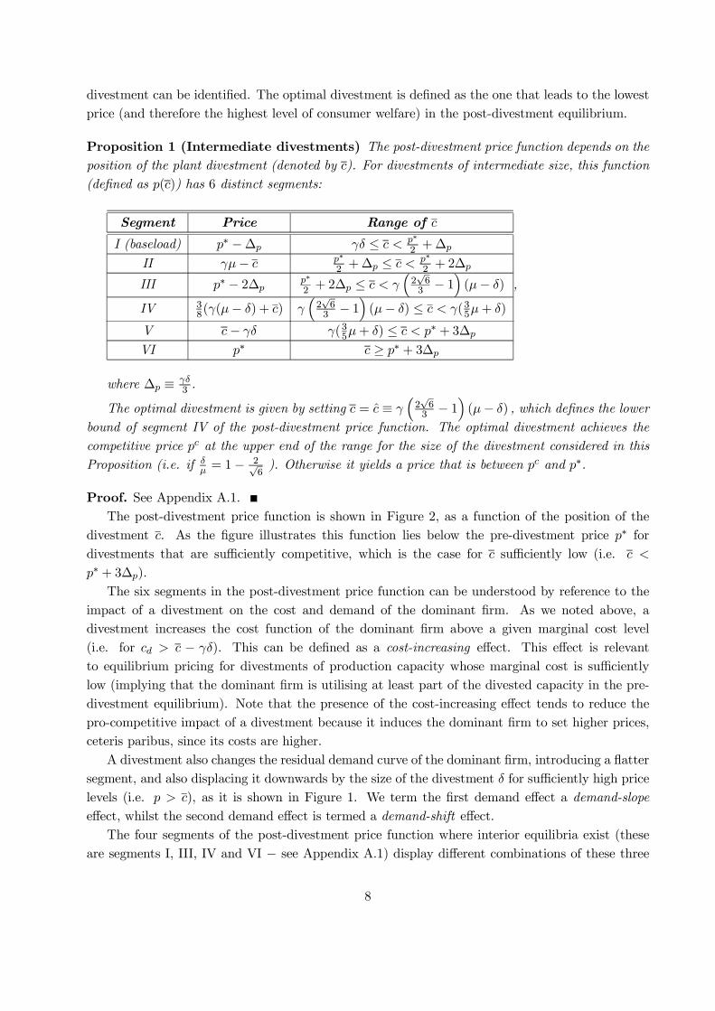
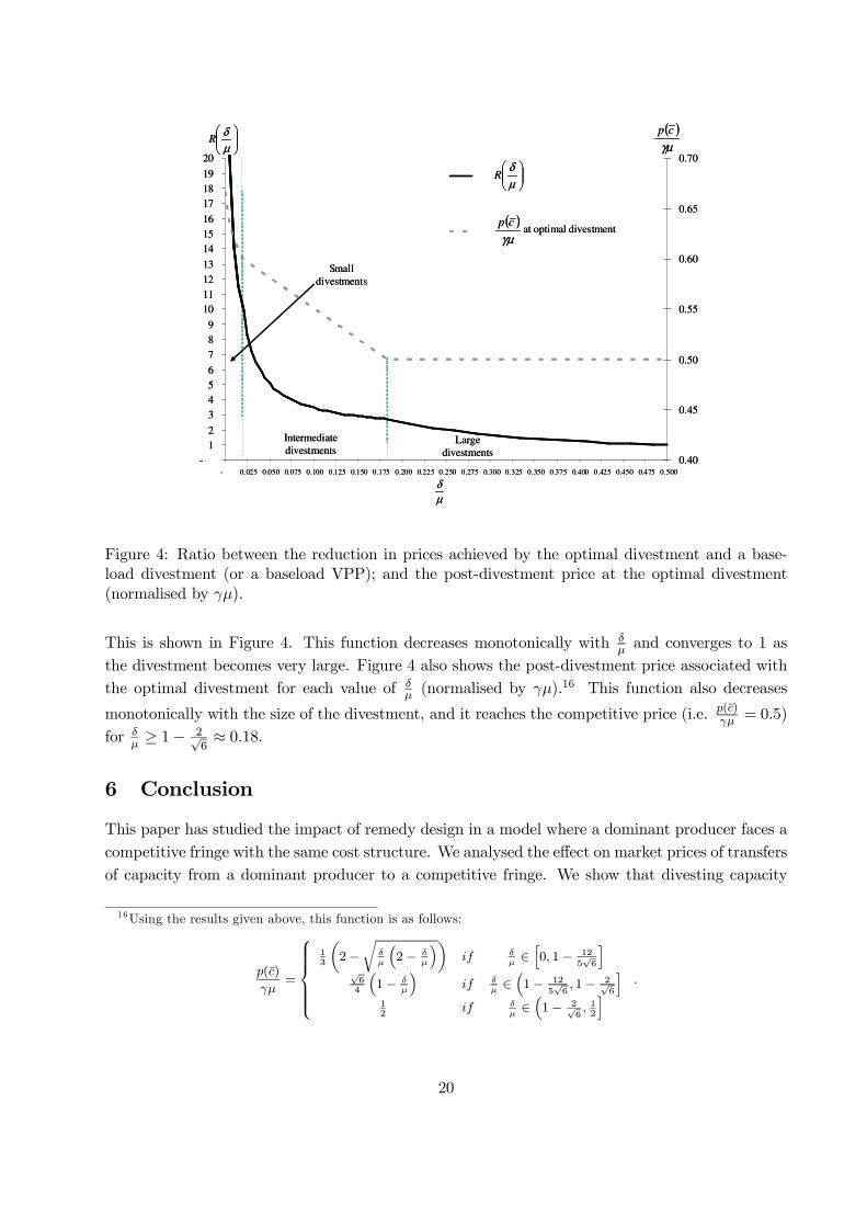
Figure 4: Ratio between the reduction in prices achieved by the optimal divestment and a base-load divestment (or a baseload VPP); and the post-divestment price at the optimal divestment(normalised by γµ).

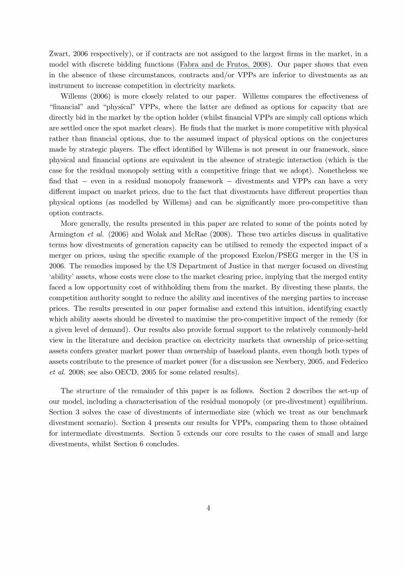
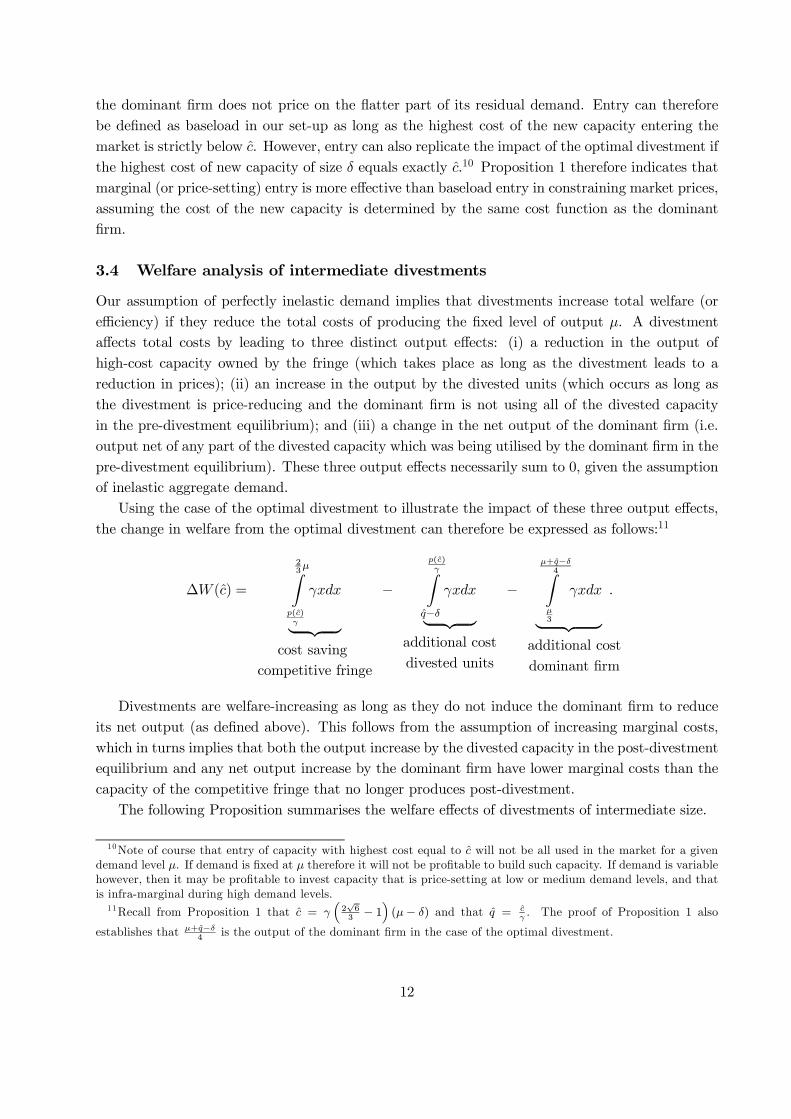
This is shown in Figure 4. This function decreases monotonically with δµand converges to 1 as

the divestment becomes very large. Figure 4 also shows the post-divestment price associated withthe optimal divestment for each value of δ

µ (normalised by γµ).16 This function also decreases

monotonically with the size of the divestment, and it reaches the competitive price (i.e. p(c)γµ

= 0.5)for δ

µ≥ 1− 2√

6≈ 0.18.

6 Conclusion

This paper has studied the impact of remedy design in a model where a dominant producer faces acompetitive fringe with the same cost structure. We analysed the effect on market prices of transfersof capacity from a dominant producer to a competitive fringe. We show that divesting capacity

16Using the results given above, this function is as follows:

p(c)

γµ=

13

(2−

√δµ

(2− δ

µ

))if δ

µ∈

[0, 1− 12

5√6

]

√64

(1− δ

µ

)if δ

µ∈

(1− 12

5√6, 1− 2√

6

]

12

if δµ∈

(1− 2√

6, 12

].

20

that is marginal (or price-setting) in the post-divestment equilibrium can be several fold moreeffective in reducing prices that an equivalent release of baseload capacity. In order to maximisethe effectiveness of the divestment from a consumer welfare perspective, the divested capacityneeds to include assets which are sufficiently competitive to impose a competitive constraint onthe dominant firm but whose costs are not too low so as to induce the dominant producer toaccept a larger loss in its output and keep prices high. In the optimal post-divestment equilibrium(for intermediate and large divestments), the cost range of the divested capacity needs to spanthe post-divestment price (implying that some but not all of the divested capacity produces inequilibrium). We also find that the optimal divestment from the perspective of consumer welfareis always efficiency-increasing.

We have also compared the effectiveness of divestments to that of VPP schemes. We establishedthat the effectiveness of VPPs is maximised when all of the options which are sold are exercised.This is achieved by setting a sufficiently low exercise price. In this case, the VPP reduces prices asmuch as a divestment of baseload generation of the same size. Given that the optimal divestmentis several-fold more effective than a baseload divestment, our findings also imply that divestmentscan be significantly more pro-competitive than VPPs (if the divested plants are selected optimally).Whilst VPPs may be preferred to a divestment because of other reasons (e.g. ease of implementa-tion, divisibility, and reversibility), our results show that relying on VPPs as a remedy instead ofusing divestments can lead to a significant reduction in the effectiveness of the intervention from amarket power mitigation perspective.

Our findings have a direct policy relevance, given that divestments and VPPs are frequentlyaccepted by competition authorities as remedies in antitrust cases relating to the electricity sector.Our results are also relevant to the evaluation of merger effects in power generation markets, sincedivestments are the exact opposite of a merger. The findings of this paper imply that a merger wherea portfolio generator buys price-setting capacity from a smaller competitor can have significantlygreater effect on prices than one where additional baseload capacity is purchased instead. Thiscan be interpreted as meaning that the competitive constraint exercised by price-setting capacityis much greater than that imposed by baseload generation. By the same token, our results indicatethat the price-increasing effect of the acquisition of a given volume of baseload generation by a firmwith market power can be remedied by significantly smaller divestments of price-setting capacity.Finally, our results also imply that the entry of price-setting independent capacity can constrainprices significantly more than the entry of low-cost plants.

Possible extensions of the work presented in this paper include the analysis of cases with variabledemand levels (which is relevant to electricity markets)17, and with oligopoly interaction. Obtaininganalytical results for standard oligopoly models (e.g. Cournot or Supply Function Equilibria) maybe a challenge in our set-up, given the cost discontinuities created by the divestments of generationcapacity. We expect however that the core intuitions developed in this paper would also extend tosuch models, given the general nature of the cost and demand effects that we identify.

Finally, whilst the set-up employed in this paper is developed with the electricity generationmarket in mind, our results also extend to other industries with homogenous products and increasing

17For a discussion of the case with variable demand see Federico and López (2009).

21

cost functions (e.g. mining).

References

[1] Allaz B. and J.-L. Vila, 1993, “Cournot Competition, Forward Markets and Efficiency", Jour-nal of Economic Theory, 59, 1-16.

[2] Armington, E., E. Emch and K. Heyer, 2006, “Economics at the Antitrust Division", Reviewof Industrial Organization, 29, 305-326.

[3] Bushnell, J., 2007, “Oligopoly Equilibria in Electricity Contract Markets", Journal of Regula-tory Economics, 32, 225-245.

[4] Gilbert, R. and D. Newbery, 2008, “Analytical Screens for Electricity Mergers", Review ofIndustrial Organization, 32, 217-239.

[5] Green, R, 1996, “Increasing Competition in the British Electricity Spot Market", The Journalof Industrial Economics, 44, 205-216.

[6] Green, R., 1999, “The Electricity Contract Market in England and Wales", The Journal ofIndustrial Economics, 47, 107-124.

[7] Fabra, N. and M.A. de Frutos, 2008, “On the Impact of Forward Contract Obligations inMulti-Unit Auctions", CEPR Working Paper.

[8] Federico, G., X. Vives and N. Fabra, 2008, Competition and Regulation in the Spanish Gas andElectricity Markets, Reports of the Public-Private Sector Research Centre, 1, IESE BusinessSchool.

[9] Federico, G. and A. L. López, 2009, “Selecting effective divestments in electricity generationmarkets", mimeo, IESE Business School (SP-SP).

[10] Newbery, D., 1998, “Competition, Contracts and Entry in the Electricity Spot Markets", TheRand Journal of Economics, 29, 726-749.

[11] Newbery, D., 2005, “Electricity Liberalisation in Britain: the Quest for a Satisfactory Whole-sale Market Design", Energy Journal, 26, Special Issue, 43-70.

[12] OECD, 2005, “Competition Issues in the Electricity Sector. Background Note", OECD Journalof Competition Law and Policy, 6, 97-162.

[13] Schultz, C., 2007, “Virtual Capacity and Competition", mimeo.

[14] Willems, B., 2006, “Virtual Divestitures, Will they make a Difference?: Cournot Competition,Options Markets and Efficiency", CSEM WP 150.

22

[15] Wolak, F. and S. McRae, 2008, “Merger Analysis in Restructured Electricity Supply Industries:The Proposed PSEG and Exelon Merger (2006)", in J. Kwoka and L. White (eds.), TheAntitrust Revolution: Economics, Competition and Policy, Oxford University Press.

[16] Zhang, Y. and G. Zwart, 2006, “Market Power Mitigation, Contracts and Contract Duration",mimeo.

A Appendix

A.1 Proof of Proposition 1

This Proposition relates to the case where δµ∈

(1− 12

5√6, 1− 2√

6

]. The dominant firm’s post-

divestment marginal cost is defined by the following two-step function:

cd =

{γqd if qd < q

′ − δγ(qd + δ) if qd ≥ q′ − δ

,

while the competitive fringe’s post-divestment marginal cost function is defined by the followingthree-step function:

cf =

γ(µ− qd − δ) if qd < µ− q′ − δγ2 (µ+ q

′ − qd − δ) if µ− q′ − δ ≤ qd ≤ µ− q′ + δγ(µ− qd) if qd > µ− q′ + δ

.

As the model is discontinuous we have to study the firm’s maximization problem in each ofthe regions defined by q′ (and δ). The proof proceeds in two steps. First, we will derive thenecessary and feasibility conditions for the equilibrium existence in each of these regions. A uniquecandidate equilibrium can exist inside each region since the model is linear. Second, we will studythe existence of profitable deviations at each candidate equilibrium and equilibria at the regionswhere the feasibility conditions are not satisfied.

Necessary and feasibility conditions for interior equilibria

Case I (baseload divestment): in this region the dominant firm and the competitive fringeof firms produce, respectively, at a higher and lower marginal cost than in the pre-divestment case,i.e., cd = γ(qd+ δ) and cf = γ(µ− qd−δ). The dominant firm maximises πId = p

IqId− γ2 (q

Id)2−γδqId

with respect to qId and subject to pI = cf , which yields qId = q∗d − 2

3δ, implying that pI = p∗ − γδ3 .

The feasibility conditions are qId < µ− q′− δ and qId > q′− δ, thus q′ < 13 min{2µ− δ, µ+ δ}. Since

δ < µ2 this condition reduces to: q′ < µ+δ

3 .Case III: the dominant firm produces at the pre-divestment marginal cost, while the com-

petitive fringe produces at a lower marginal cost, i.e., cd = γqd and cf = γ(µ − qd − δ). Thus,pIII = γ(µ− qd− δ) and πIIId = pIIIqIIId − γ

2 (qIIId )2. The first-order condition yields qIIId = q∗d − δ

3 ,implying that pIII = p∗− 2γδ

3 . The feasibility conditions are qIIId < µ−q′−δ and qIIId ≤ q′−δ, whichfor δ < µ

4 (which is the case for the range of δ that we consider) boil down to: µ+2δ3 ≤ q′ < 2(µ−δ)

3 .

Conversely, if δ ≥ µ4 , no equilibrium exists in the region of Case III.

23

Case IV : the dominant firm produces at the pre-divestment marginal cost, while the com-petitive fringe produces at the flatter part of its marginal cost function, i.e., cd = γqd andcf =

γ2 (µ + q

′ − qd − δ). Thus, pIV = γ2 (µ + q

′ − qd − δ) and πIVd = pIV qIVd − γ2 (q

IVd )2. From

the first-order condition we obtain qIVd = µ+q′−δ4 , so pIV = 3

8(γ(µ− δ) + c). The feasibility condi-tion µ − q′ − δ ≤ qIVd ≤ µ − q′ + δ can be rewritten as (3/5)(µ − δ) ≤ q′ ≤ (3/5)µ + δ, and thefeasibility condition qIVd ≤ q′ − δ can be rewritten as q′ ≥ δ + µ/3.

Notice that 35(µ − δ) ≥ δ +

µ3 if δ ≤ µ

6 . In such a case the feasibility conditions boil down to:35(µ− δ) ≤ q′ ≤ 3

5µ+ δ.

Conversely, if δ > µ6 , the feasibility conditions reduce to: δ + µ

3 ≤ q′ ≤ 35µ+ δ.

Case V I: the dominant firm and the competitive fringe of firms produce at the pre-divestmentmarginal cost, i.e., ci = γqi for i = d, f . Thus, the first-order condition yields the same result as inthe pre-divestment case: qV Id = q∗d and p

V I = p∗. Here, the feasibility conditions are qV Id > µ−q′+δor, equivalently, q′ > 2

3µ + δ, and qV Id ≤ q′ − δ, or, equivalently, q′ ≥ µ

3 + δ. Thus, we have that:q′ > 2

3µ+ δ.

Infeasible cases or sub-optimal cases

Case i: cd = γ(qd + δ) and cf =γ2 (µ + q

′ − qd − δ). The first-order condition yields qd =14(µ+ q

′−3δ). The feasibility condition µ− q′− δ ≤ qd ≤ µ− q′+ δ implies that 3µ−δ5 ≤ q′ ≤ 3µ+7δ5 ,

while the feasibility condition qd > q′ − δ implies that q′ < µ+δ3 . Since µ+δ

3 < 3µ+7δ5 , the two

conditions reduce to 3µ−δ5 ≤ q′ < µ+δ

3 . However µ+δ3 > 3µ−δ

5 holds only if δ > µ2 .

Case ii: cd = γ(qd + δ) and cf = γ(µ− qd). From the first-order condition we have qd =µ−δ3 .

The condition qd > µ− q′+ δ can be rewritten as q′ > 23(µ+2δ), while qd > q

′− δ can be rewrittenas q′ < µ+2δ

3 . Therefore, we have that 23(µ+ 2δ) < q

′ < µ+2δ3 , which is a contradiction.

Case iii: the post-divestment marginal cost curve passes through the second jump of themarginal revenue curve. If so, the higher value of the marginal revenue function at qd = µ−q′+δ, i.e.,γ2 (µ+q

′−δ)−γ(µ−q′+δ), must be higher than the corresponding marginal cost: γ(µ−q′+δ+δ). Thisrequires that q′ > 3µ+7δ

5 . Also, the lower value of the marginal revenue function at qd = µ− q′ + δ,i.e., γ(µ− 2(µ− q′ + δ)), must be lower than marginal cost: γ(µ− q′ + δ + δ). This requires that2µ+4δ3 > q′. Thus, 3µ+7δ5 < q′ < 2

3(µ + 2δ), which holds since δ < µ. In addition, we need thatq′ − δ < µ− q′ + δ, i.e. q′ < µ

2 + δ. Nevertheless,µ2 + δ <

3µ+7δ5 holds, which is a contradiction.

Case iv: the third segment of the marginal revenue curve passes through the jump of themarginal cost curve. This requires that γ((q′ − δ) + δ) > γ(µ− 2(q′ − δ)), i.e., q′ > µ+2δ

3 , and thatγ(µ− 2(q′− δ)) > γ(q′− δ), i.e. q′ < µ

3 + δ. Both conditions can be rewritten as µ+2δ3 < q′ < µ3 + δ.

In addition, we need that q′− δ > µ− q′+ δ, or, equivalently, if q′ > µ2 + δ. However,

µ3 + δ <

µ2 + δ

holds.Case v: The flat part of the marginal revenue curve passes through the jump of the marginal cost

curve. If so, the flat part of the marginal revenue curve at qd = q′−δ, i.e., γ2 (µ+q′−δ)−γ(q′−δ), mustbe lower than the post-divestment marginal cost: γ (qd + δ) = γq′. This requires that q′ > µ+δ

3 .Also, the marginal revenue curve at qd = q′ − δ must be higher than the pre-divestment marginalcost: γ(q′−δ). This requires that q′ < µ

3+δ. In addition, we need that µ−q′+δ < q′−δ < µ−q′+δ,or, equivalently, µ2 < q

′ < µ2 + δ. These four conditions can be rewritten as: max{µ2 ,

µ+δ3 } < q′ ≤

min{µ2 + δ,

µ3 + δ

}or µ

2 < q′ ≤ µ3 + δ provided that δ < µ

2 . Note that µ3 + δ >

µ2 if and only if

24

3

δµ +

3

2δµ +

( )δµµ

δ −≤5

3:

6if

δµµ

δ +≥5

3:

25if

( )δµ −3

2

δµµ

δ +<5

3:

25if

δµ +3

2

Case I Case IICase III

Case IV

3:

6

µδ

µδ +>if

Case V

Case VI

q’3

δµ +

3

2δµ +

( )δµµ

δ −≤5

3:

6if

δµµ

δ +≥5

3:

25if

( )δµ −3

2

δµµ

δ +<5

3:

25if

δµ +3

2

Case I Case IICase III

Case IV

3:

6

µδ

µδ +>if

Case V

Case VI

q’

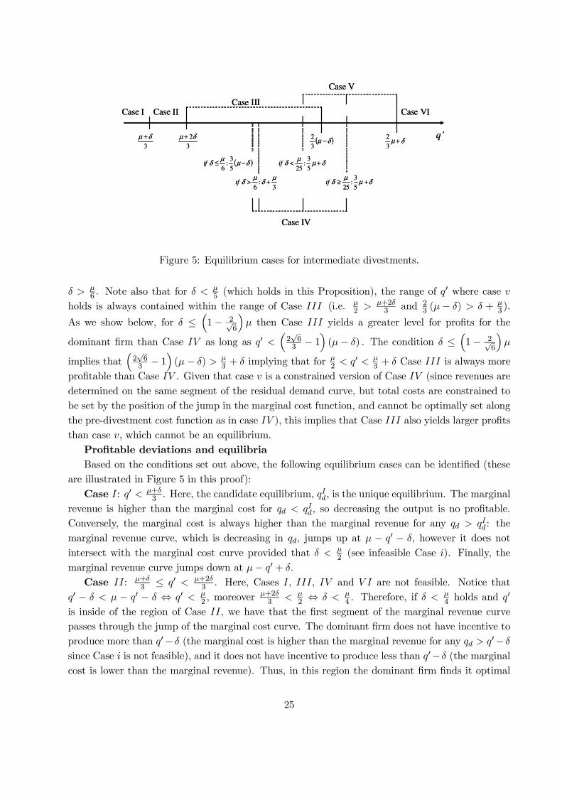
Figure 5: Equilibrium cases for intermediate divestments.

δ > µ6 . Note also that for δ < µ

5 (which holds in this Proposition), the range of q′ where case vholds is always contained within the range of Case III (i.e. µ

2 >µ+2δ3 and 2

3 (µ− δ) > δ + µ3 ).

As we show below, for δ ≤(1− 2√

6

)µ then Case III yields a greater level for profits for the

dominant firm than Case IV as long as q′ <(2√63 − 1

)(µ− δ) . The condition δ ≤

(1− 2√

6

)µ

implies that(2√63 − 1

)(µ− δ) > µ

3 + δ implying that for µ2 < q

′ < µ3 + δ Case III is always more

profitable than Case IV . Given that case v is a constrained version of Case IV (since revenues aredetermined on the same segment of the residual demand curve, but total costs are constrained tobe set by the position of the jump in the marginal cost function, and cannot be optimally set alongthe pre-divestment cost function as in case IV ), this implies that Case III also yields larger profitsthan case v, which cannot be an equilibrium.

Profitable deviations and equilibria

Based on the conditions set out above, the following equilibrium cases can be identified (theseare illustrated in Figure 5 in this proof):

Case I: q′ < µ+δ3 . Here, the candidate equilibrium, qId, is the unique equilibrium. The marginal

revenue is higher than the marginal cost for qd < qId, so decreasing the output is no profitable.Conversely, the marginal cost is always higher than the marginal revenue for any qd > qId: themarginal revenue curve, which is decreasing in qd, jumps up at µ − q′ − δ, however it does notintersect with the marginal cost curve provided that δ < µ

2 (see infeasible Case i). Finally, themarginal revenue curve jumps down at µ− q′ + δ.

Case II: µ+δ3 ≤ q′ < µ+2δ

3 . Here, Cases I, III, IV and V I are not feasible. Notice thatq′ − δ < µ − q′ − δ ⇔ q′ < µ

2 , moreover µ+2δ3 < µ

2 ⇔ δ < µ4 . Therefore, if δ < µ

4 holds and q′

is inside of the region of Case II, we have that the first segment of the marginal revenue curvepasses through the jump of the marginal cost curve. The dominant firm does not have incentive toproduce more than q′− δ (the marginal cost is higher than the marginal revenue for any qd > q′− δsince Case i is not feasible), and it does not have incentive to produce less than q′−δ (the marginalcost is lower than the marginal revenue). Thus, in this region the dominant firm finds it optimal

25

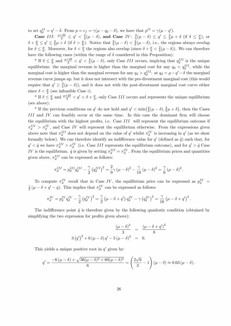
to set qIId = q′ − δ. From p = cf = γ(µ− qd − δ), we have that pII = γ(µ− q′).Case III: µ+2δ

3 ≤ q′ < 23(µ − δ), and Case IV : 3

5(µ − δ) ≤ q′ ≤ 35µ + δ (if δ ≤ µ

6 ), orδ + µ

3 ≤ q′ ≤ 35µ + δ (if δ > µ

6 ). Notice that 35(µ − δ) < 2

3(µ − δ), i.e., the regions always overlapfor δ ≤ µ

6 . Moreover, for δ < µ5 the regions also overlap (since δ+ µ

3 <23(µ− δ)). We can therefore

have the following cases (within the range of δ considered in this Proposition):* If δ ≤ µ

6 and µ+2δ3 < q′ < 3

5(µ − δ), only Case III occurs, implying that qIIId is the uniqueequilibrium: the marginal revenue is higher than the marginal cost for any qd < qIIId , while themarginal cost is higher than the marginal revenue for any qd > qIIId : at qd = µ−q′−δ the marginalrevenue curve jumps up, but it does not intersect with the pre-divestment marginal cost (this wouldrequire that q′ ≥ 3

5(µ − δ)), and it does not with the post-divestment marginal cost curve eithersince δ < µ

2 (see infeasible Case i).* If δ ≤ µ

6 and µ+2δ3 < q′ < δ + µ

3 , only Case III occurs and represents the unique equilibrium(see above).

* If the previous conditions on q′ do not hold and q′ < min{23(µ− δ), 35µ+ δ}, then the CasesIII and IV can feasibly occur at the same time. In this case the dominant firm will choosethe equilibrium with the highest profits, i.e. Case III will represent the equilibrium outcome ifπIIId > πIVd , and Case IV will represent the equilibrium otherwise. From the expressions givenabove note that πIIId does not depend on the value of q′ whilst πIVd is increasing in q′ (as we showformally below). We can therefore identify an indifference value for q′ (defined as q) such that, forq′ < q we have πIIId > πIVd (i.e. Case III represents the equilibrium outcome), and for q′ > q CaseIV is the equilibrium. q is given by setting πIIId = πIVd . From the equilibrium prices and quantitiesgiven above, πIIId can be expressed as follows:

πIIId = pIIId qIIId − γ2

(qIIId

)2=2

9γ (µ− δ)2 − γ

18(µ− δ)2 = γ

6(µ− δ)2 .

To compute πIVd recall that in Case IV , the equilibrium price can be expressed as pIVd =γ2 (µ− δ + q′ − q). This implies that πIVd can be expressed as follows:

πIVd = pIVd qIVd − γ

2

(qIVd

)2=γ

2

(µ− δ + q′

)qIVd − γ

(qIVd

)2=γ

16

(µ− δ + q′

)2 .

The indifference point q is therefore given by the following quadratic condition (obtained bysimplifying the two expression for profits given above):

(µ− δ)23

=(µ− δ + q′)2

8

3(q′)2+ 6 (µ− δ) q′ − 5 (µ− δ)2 = 0.

This yields a unique positive root in q′ given by:

q′ =−6 (µ− δ) +

√36(µ− δ)2 + 60(µ− δ)26

=

(2√6

3− 1

)(µ− δ) ≈ 0.63 (µ− δ) .

26

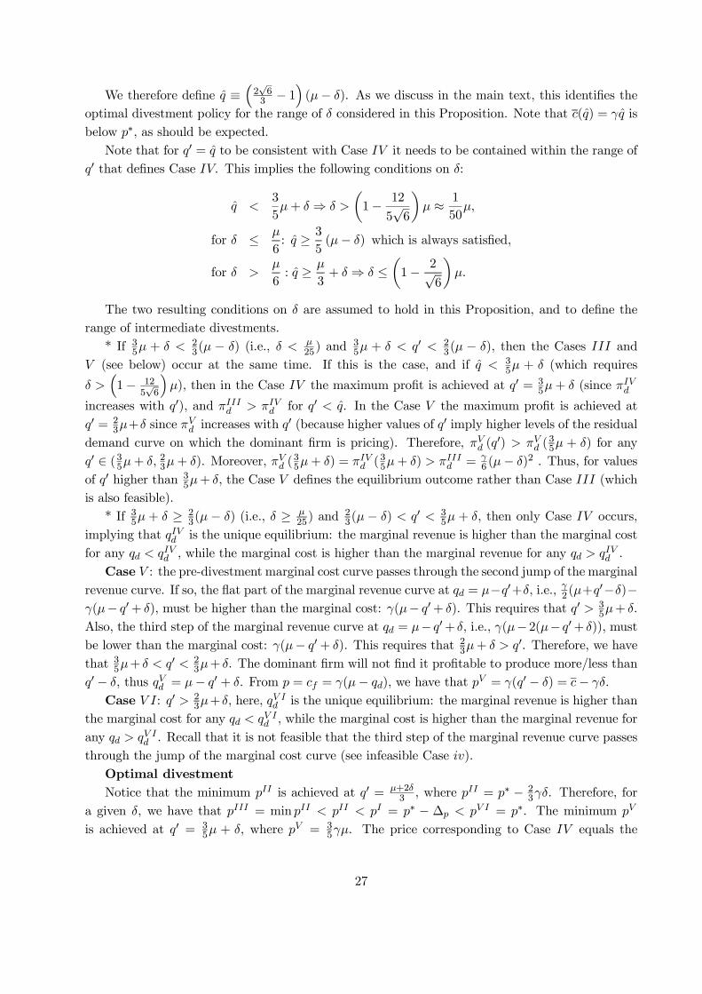
We therefore define q ≡(2√63 − 1

)(µ− δ). As we discuss in the main text, this identifies the

optimal divestment policy for the range of δ considered in this Proposition. Note that c(q) = γq isbelow p∗, as should be expected.

Note that for q′ = q to be consistent with Case IV it needs to be contained within the range ofq′ that defines Case IV. This implies the following conditions on δ:

q <3

5µ+ δ ⇒ δ >

(1− 12

5√6

)µ ≈ 1

50µ,

for δ ≤ µ

6: q ≥ 3

5(µ− δ) which is always satisfied,

for δ >µ

6: q ≥ µ

3+ δ ⇒ δ ≤

(1− 2√

6

)µ.

The two resulting conditions on δ are assumed to hold in this Proposition, and to define therange of intermediate divestments.

* If 35µ + δ <

23(µ − δ) (i.e., δ <

µ25) and 3

5µ + δ < q′ < 23(µ − δ), then the Cases III and

V (see below) occur at the same time. If this is the case, and if q < 35µ + δ (which requires

δ >(1− 12

5√6

)µ), then in the Case IV the maximum profit is achieved at q′ = 3

5µ+ δ (since πIVdincreases with q′), and πIIId > πIVd for q′ < q. In the Case V the maximum profit is achieved atq′ = 2

3µ+δ since πVd increases with q′ (because higher values of q′ imply higher levels of the residual

demand curve on which the dominant firm is pricing). Therefore, πVd (q′) > πVd (

35µ + δ) for any

q′ ∈ (35µ+ δ, 23µ+ δ). Moreover, πVd (35µ+ δ) = π

IVd (

35µ+ δ) > π

IIId = γ

6 (µ− δ)2 . Thus, for valuesof q′ higher than 3

5µ+ δ, the Case V defines the equilibrium outcome rather than Case III (whichis also feasible).

* If 35µ + δ ≥ 23(µ − δ) (i.e., δ ≥

µ25) and 2

3(µ − δ) < q′ < 35µ + δ, then only Case IV occurs,

implying that qIVd is the unique equilibrium: the marginal revenue is higher than the marginal costfor any qd < qIVd , while the marginal cost is higher than the marginal revenue for any qd > qIVd .

Case V : the pre-divestment marginal cost curve passes through the second jump of the marginalrevenue curve. If so, the flat part of the marginal revenue curve at qd = µ−q′+δ, i.e., γ2 (µ+q′−δ)−γ(µ− q′+ δ), must be higher than the marginal cost: γ(µ− q′+ δ). This requires that q′ > 3

5µ+ δ.Also, the third step of the marginal revenue curve at qd = µ− q′+ δ, i.e., γ(µ−2(µ− q′+ δ)), mustbe lower than the marginal cost: γ(µ− q′ + δ). This requires that 2

3µ+ δ > q′. Therefore, we have

that 35µ+ δ < q′ < 2

3µ+ δ. The dominant firm will not find it profitable to produce more/less thanq′ − δ, thus qVd = µ− q′ + δ. From p = cf = γ(µ− qd), we have that pV = γ(q′ − δ) = c− γδ.

Case V I: q′ > 23µ+ δ, here, q

V Id is the unique equilibrium: the marginal revenue is higher than

the marginal cost for any qd < qV Id , while the marginal cost is higher than the marginal revenue forany qd > qV Id . Recall that it is not feasible that the third step of the marginal revenue curve passesthrough the jump of the marginal cost curve (see infeasible Case iv).

Optimal divestment

Notice that the minimum pII is achieved at q′ = µ+2δ3 , where pII = p∗ − 2

3γδ. Therefore, fora given δ, we have that pIII = min pII < pII < pI = p∗ − ∆p < pV I = p∗. The minimum pV

is achieved at q′ = 35µ + δ, where p

V = 35γµ. The price corresponding to Case IV equals the

27

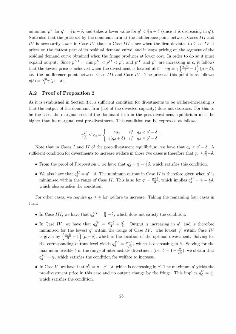
minimum pV for q′ = 35µ+ δ, and takes a lower value for q′ < 3

5µ+ δ (since it is decreasing in q′).Note also that the price set by the dominant firm at the indifference point between Cases III andIV is necessarily lower in Case IV than in Case III since when the firm deviates to Case IV itprices on the flattest part of its residual demand curve, and it stops pricing on the segment of theresidual demand curve obtained when the fringe produces at lower cost. In order to do so it mustexpand output. Since pIII = min pII < pII < pI , and pIV and pV are increasing in c, it followsthat the lowest price is achieved when the divestment is located at c = γq ≡ γ

(2√63 − 1

)(µ− δ),

i.e. the indifference point between Case III and Case IV . The price at this point is as follows:p(c) =

√64 γ (µ− δ).

A.2 Proof of Proposition 2

As it is established in Section 3.4, a sufficient condition for divestments to be welfare-increasing isthat the output of the dominant firm (net of the divested capacity) does not decrease. For this tobe the case, the marginal cost of the dominant firm in the post-divestment equilibrium must behigher than its marginal cost pre-divestment. This condition can be expressed as follows:

γµ

3≤ cd =

{γqd if qd < q

′ − δγ(qd + δ) if qd ≥ q′ − δ

.

Note that in Cases I and II of the post-divestment equilibrium, we have that qd ≥ q′ − δ. Asufficient condition for divestments to increase welfare in those two cases is therefore that qd ≥ µ

3−δ.

• From the proof of Proposition 1 we have that qId =µ3 − 2

3δ, which satisfies this condition.

• We also have that qIId = q′− δ. The minimum output in Case II is therefore given when q′ isminimised within the range of Case II. This is so for q′ = µ+δ

3 , which implies qIId = µ3 − 2

3δ,which also satisfies the condition.

For other cases, we require qd ≥ µ3 for welfare to increase. Taking the remaining four cases in

turn:

• In Case III, we have that qIIId = µ3 − δ

3 , which does not satisfy the condition.

• In Case IV , we have that qIVd = µ−δ4 + q′

4 . Output is increasing in q′, and is thereforeminimised for the lowest q′ within the range of Case IV . The lowest q′ within Case IVis given by

(2√63 − 1

)(µ− δ), which is the location of the optimal divestment. Solving for

the corresponding output level yields qIVd = µ−δ√6, which is decreasing in δ. Solving for the

maximum feasible δ in the range of intermediate divestment (i.e. δ = 1− 2√6), we obtain that

qIVd = µ3 , which satisfies the condition for welfare to increase.

• In Case V , we have that qVd = µ−q′+δ, which is decreasing in q′. The maximum q′ yields thepre-divestment price in this case and no output change by the fringe. This implies qVd =

µ3 ,

which satisfies the condition.

28

• The condition is trivially satisfied in Case V I, where the divestment has no impact on marketoutcomes.

The only case where divestments can lead to a reduction in welfare is therefore Case III. Inthis case, the change in welfare is given by the following expression (recalling that pIII = p∗− 2

3γδ):

∆W III =

23µ∫

23µ− 2

3δ

γxdx+

µ3∫

µ3− δ3

γxdx−q′∫

q′−δ

γxdx.

This simplifies to the following: ∆W III = γδ(29δ +

59µ− q′

), which is decreasing in q′. Substi-

tuting for the highest value of q′ that is feasible in Case III (i.e. q′ =(2√63 − 1

)(µ− δ) ) , yields

the following condition for ∆W III ≥ 0 :

δ

µ≥ 6

√6− 14

6√6− 7

≈ 0.09,

which is within the range of δµconsidered in the case of intermediate divestments. This proves that

for δµ< 6

√6−14

6√6−7 − and q′ high enough − divestments can reduce welfare.

A.3 Proof of Proposition 3

Case I (the option is always exercised)

The profit of the dominant firm is πd = pqd − γ2 (qd)

2 +∫ q′q′−δ γxdx − pδ where p = γ(µ − qd).

Simplifying, we obtainπd = pqd −

γ

2(qd)

2 +γ

2(−δ2 + 2q′δ)− pδ.

The first-order derivative yields qd =µ+δ3 , and therefore p = γ

(2µ−δ3

). The feasibility conditions

are that p > γq′ and q′ ≥ δ. The former implies: q′ < 2µ−δ3 ⇒ c < p∗ − γδ

3 . To satisfy the secondcondition we require δ ≤ µ

2 .

Case II (only part of the option is exercised)

The profit of the dominant firm is πd = pqd − γ2 (qd)

2 +∫ µ−qdq′−δ γxdx− p [(µ− qd)− (q′ − δ)] ,where

we have used that p/γ = qf = µ− qd. Simplifying,

πd = γ(µ− qd)(2qd + q′ − µ− δ) +γ

2(µ2 + 2q′δ − 2µqd − q′ − δ2).

The first-order condition yields qd =µ2 −

(q′−δ4

)and therefore p = γ

(µ2 +

q′−δ4

). For this solution

to be an equilibrium the following two feasibility conditions must hold i) qd > 0, or q′ < 2µ+ δ; ii)γ(q′ − δ) < p < γq′, this condition can be rewritten as

2µ− δ3

< q′ <2µ

3+ δ,

29

which is stricter than condition i. The equivalent condition for c is: p∗ − γδ3 < c < p

∗ + γδ.

A.4 Proof of Proposition 4

The welfare impact of a baseload VPP (which we define as ∆WB) is the same as the one of abaseload divestment. It is given by the reduction in costs faced by the competitive fringe due toits output reduction, minus the increase in cost for the dominant firm, due to its output increase:

∆WB =

23µ∫

23µ− δ

3

γxdx−

µ+δ3∫

µ3

γxdx,

which simplifies to γδ9 (µ− δ).

Recall that at the optimal divestment the price and the output are given by p(c) =√64 γ (µ− δ)

and qIVd = µ−δ√6. These results imply that the welfare impact of the optimal divestment (which we

define as ∆W ) is given by the following expression:

∆W =

23µ∫

√64(µ−δ)

γxdx−

µ−δ√6∫

µ3

γxdx−

√64(µ−δ)∫

(2√6

3−1)(µ−δ)−δ

γxdx

= γ

518µ2 − 11(µ− δ)

2

24+

((2√63 − 1

)(µ− δ)− δ

)

2

= γ

[(119

72− 23

√6

)µ2 +

7

8δ2 −

(7

4− 23

√6

)δµ

].

We have that

∆W −∆WB = γ

[(119

72− 23

√6

)µ2 +

(7

8+1

9

)δ2 −

(7

4− 23

√6 +

1

9

)δµ

]

= γ

[(119

72− 23

√6

)µ2 +

71

72δ2 −

(67

36− 23

√6

)δµ

].

The gradient of ∆W −∆WB is

� (µ, δ) =(d

dµ

(∆W −∆WB

),d

dδ

(∆W −∆WB

)),

with �(0, 0) = 0. The Hessian matrix of ∆W −∆WB is

H(∆W −∆WB) =

[2(11972 − 2

3

√6)−(6736 − 2

3

√6)

−(6736 − 2

3

√6)

2(7172

)],

which is positive definite. Hence, µ = δ = 0 is a global minimum, where ∆W −∆WB = 0. For any

30

positive µ > 0 and δ > 0, we thus have that ∆W −∆WB > 0.

A.5 Proof of Proposition 5

From the proof of Proposition 1 we have that for δµ ∈ (0, 1− 12

5√6) the cases i, ii, iii, iv and v are

not feasible (case v requires that δ > µ/6), whereas Cases I, II, III, IV , V and V I are feasibledepending on the location of q′. Using the proof of Proposition 1, we have that, for a given q′,

• if q′ < µ+δ3 , then qId is the unique equilibrium.

• if µ+δ3 ≤ q′ < µ+2δ3 , then qIId is the unique equilibrium.

• if µ+2δ3 ≤ q′ < 35(µ− δ), then qIIId is the unique equilibrium.

• if 35(µ − δ) ≤ q′ ≤ 35µ + δ, then Cases III and IV overlap. From above, however, we have

that q, which is given by πIIId = πIVd , is not contained in the range of q′ that defines CaseIV . As case i is not feasible, here qIIId is the unique equilibrium.

• if 35µ + δ < q′ < 2

3(µ− δ), then Cases III and V overlap (since δ < µ/25). In this case thedominant firm will choose the equilibrium that yields the highest profit. Thus, Case III isthe equilibrium outcome if πIIId > πVd , and Case V is the equilibrium otherwise. Recall thatπIIId = γ

6 (µ− δ)2, whereas πVd is increasing in q′:

πVd = γ(q′ − δ)(µ− q′ + δ)− γ

2(µ− q′ + δ)2.

Let q′ be a value for q′ so that πIIId = πVd , then for q′ < q′ we have πIIId > πVd , and for q′ > q′

we have πVd > πIIId , provided that 3

5µ+ δ < q′ < 2

3(µ− δ). q′ is thus given by

γ(µ− q′ + δ)[(q′ − δ)− (µ− q

′ + δ)

2

]=γ

6(µ− δ)2,

which can be rewritten as

−3q′2 + 2(3δ + 2µ)q′ − 23(2µ2 + 5δ2 + 5δµ) = 0.

This yields two positive roots in q′, but only one of them is contained in the region whereCase V is feasible:18

q′ = q′ ≡ 2

3µ+ δ − 1

3

√δ(2µ− δ).

This root is contained in the region where Cases III and V overlap. This follows from thefact that πVd > π

IIId at q′ = 2

3(µ−δ), and πIIId > πVd at q′ = 35µ+δ. Since π

IIId is constant and

πVd is increasing in q′, we have that 35µ+δ < q′ < 2

3(µ−δ). The price is given by p = γ(q′−δ),thus for q′ = q′ we have that p(γq′) = p∗ − γ

3

√δ(2µ− δ).

• if 23(µ− δ) < q′ < 23µ+ δ, then only Case V applies, qVd is then the unique equilibrium.

18The second root is above the upper bound of the feasible region, i.e., 23µ+ δ +

13

√δ(2µ− δ) > 2

3 (µ− δ).

31

• if q′ > 23µ+ δ, then q

V Id is the unique equilibrium.

Notice that the minimum pII is achieved at q′ = µ+2δ3 , where pII = p∗ − 2

3γδ, and that theminimum price achieved when Case V is the only case which applies (defined as min pV ) obtainsat q′ = 2

3(µ− δ), where pV = p∗ − 53γδ. Therefore, for a given δ, the minimum prices that can be

achieved in each region satisfy min pV < minpII = pIII < pI = p∗− 13γδ < p

V I = p∗. In the regionwhere Cases III and V overlap, q′ is lower than the lower bound of the region where only CaseV exists and, moreover, pV and πVd increase with q′, thus p(γq′) < min pV . Therefore, the optimal

divestment is located at c = c ≡ γq′. Finally, R( δµ) =p∗−p(γq′)

∆p=√δ(2µ−δ)δ =

√2µδ − 1.

A.6 Proof of Proposition 6

From the proof of Proposition 1 we have that for δµ ∈ (1− 2√

6, 12 ] the Cases i, ii, iii and iv are not

feasible, whereas Cases v, I, II, III, IV , V and V I are feasible. The range where Case v applies isµ2 < q

′ < µ3+δ. As it is shown in the proof of Proposition 1, the output of the dominant firm in Case

v is given by qd = q′ − δ whilst the inverse demand curve is given by p(qd) =γ2

(µ+ q′ − δ − qd

).

This in turn implies that pv = γµ2 ≡ pc. This means that if for a given q′ Case v is the equilibrium

outcome, q′ also represents the optimal position of the divestment (though not necessarily unique),since it delivers the competitive price pc.

Using the proof of Proposition 1, we have that, for a given q′,

• if δ ≥ µ5 , then only the Case v exists, so pv is the unique equilibrium, for q′ ∈

(23 (µ− δ) ,

µ3 + δ

).

• if δ < µ5 , then Cases III and v overlap for µ

2 < q′ ≤ µ

3 + δ.

These conditions imply that if πvd > πIIId at q′ = µ3 + δ, then setting q′ = µ

3 + δ achievesthe optimal divestment. As shown in the proof of Proposition 1, πIIId = γ

6 (µ− δ)2 . Using the

expressions for price and quantity given above we also have that:

πvd =γµ

2

(q′ − δ

)− γ2

(q′ − δ

)2=γ

2

(q′ − δ

) (µ− q′ + δ

).

Setting q′ = µ3+δ we have that π

vd > π

IIId if 19µ

2 > γ6 (µ− δ)

2 , which is equivalent to 23µ2 > (µ− δ)2.

In the range of δ considered here (i.e. for δµ ∈ (1 − 2√

6, 12 ] ) this condition is satisfied, since the

right hand side of the inequality is decreasing in δ, and it equals 23µ2 for δ =

(1− 2√

6

)µ. This

proves that setting q′ = µ3 + δ achieves the optimal divestment in the range of δ

µconsidered in this

Proposition. For all other values of δ contained within the range considered in this Proposition (i.e.for δ >

(1− 2√

6

)µ), there exists a lower value for q′ so that the equilibrium price is the competitive

price. To see this, notice that

dπVddδ

= −dπVd

dq′= pc − γ(q′ − δ),

which implies that for a slight increase in δ, there exists a slight decrease in q′ so that πVd keepsconstant. By contrast, for a slight increase in δ, πIIId decreases. Therefore, for a higher δ, thereexist multiple values for q′ for which pc is the equilibrium outcome (since πVd > π

IIId ).

32

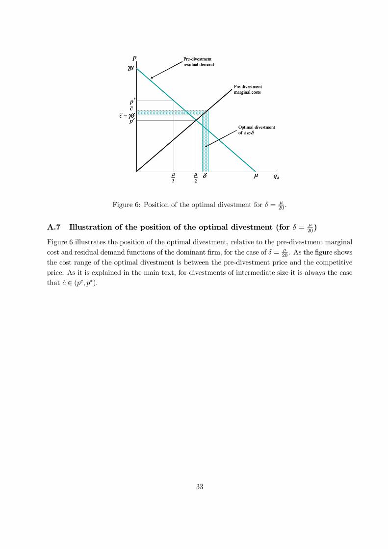
µ

γµ

Optimal divestment

of size

Pre-divestment

residual demand

2

µ

3

µ

*p

cp

Pre-divestment

marginal costs

δ

δ

dq

p

c)

γδ−c)

µ

γµ

Optimal divestment

of size

Pre-divestment

residual demand

2

µ

3

µ

*p

cp

Pre-divestment

marginal costs

δ

δ

dq

p

c)

γδ−c)

Figure 6: Position of the optimal divestment for δ = µ20 .

A.7 Illustration of the position of the optimal divestment (for δ = µ

20)

Figure 6 illustrates the position of the optimal divestment, relative to the pre-divestment marginalcost and residual demand functions of the dominant firm, for the case of δ = µ

20 . As the figure showsthe cost range of the optimal divestment is between the pre-divestment price and the competitiveprice. As it is explained in the main text, for divestments of intermediate size it is always the casethat c ∈ (pc, p∗).

33