Diversity Techniques

7. Diversity Techniques

• References:

1. Schwartz, Bennett, and Stein, “Communication Systems and Techniques”, McGraw Hill, 1966, Chapters 10-11:

- this is a classic for both analog and digital systems.

2. Proakis, “Digital Communications”, 3rd Edition, McGraw Hill, 1995, Section 14-4:

- only a subset of Ref [1] above.

3. M.Z. Win and J.H. Winters, “Exact Error Probability Expression for Hybrid Selection/Maximal-Ratio Combining in Rayleigh Fading: A Virtual Branch Technique”, Proc. IEEE Globecom, Rio de Janeiro, Brazil, Dec. 1999:

- a very interesting paper as it formulates both selection and combining under a

single framework. The receiver performs maximal ratio combining for the L (out of a total of N) branches with the largest instantaneous SNR. This generalized selection/combining strategy can be potentially used in CDMA system where the receiver searches for the L strongest multipaths and perform RAKE combining.

• In Chapters 4-6, we examined the bit error probability (BEP) performance

of BPSK and QPSK in Rayleigh flat fading channels. Generally it was pretty dismal: even with ideal coherent detection, we need a signal-to-noise ratio (SNR) of 24 dB just to hit a BEP of 310eP −= , and decreases only as

. eP

( ) 1/b oE N −

7-1

• The best way to gain major improvement is through diversity and the argument runs like this.

- Suppose you have access to several independent fading channels, each

carrying the same signal

( )s t

1( )g t1( )n t

2 ( )g t2 ( )n t

2 ( )r t

( )Ng t ( )Nn t

•••

( )Nr t

1( )r t - We know that errors on a single channel are associated with deep fades;

roughly speaking the BEP is the probability of being below some “problem SNR”.

- If we have two channels, the probability that they are both below the

problem SNR is 2eP ; with N channels, it’s N

eP .

Thus we might expect behavior like the one shown in the figure below. This would bring huge benefits; e.g., if it takes 40 dB to get 410eP −= with one channel, then only 20 dB for two channels, 10 dB for four channels

7-2

And, in fact, it does behave much like this.

)b oE N

1; slope = 1N = −

2; slope = 2N = −

4; slope = 4N = −

/ (dB

( )log eP

7.1 Sources of Diversity

• With Doppler spread, the complex gain varies with time, so repeat the information after a few multiples of 1/ df . This is time diversity. It consumes extra transmission time.

BPF2 ( )r t%

1( )r t%

LNA

IF

MIX delay

LO

7-3

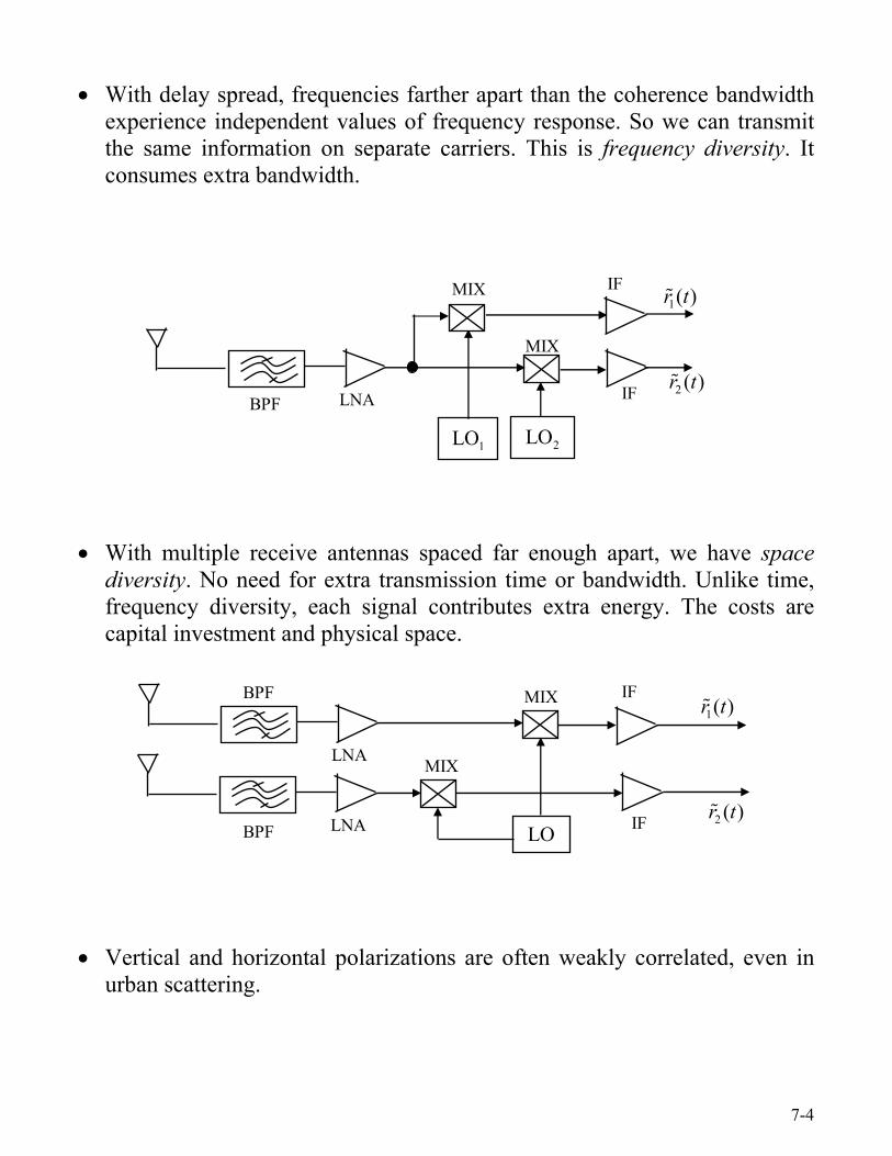
• With delay spread, frequencies farther apart than the coherence bandwidth experience independent values of frequency response. So we can transmit the same information on separate carriers. This is frequency diversity. It consumes extra bandwidth.

LNABPF IF

MIX

2 ( )r t%

1( )r t%

1LO 2LO

MIX IF • With multiple receive antennas spaced far enough apart, we have space

diversity. No need for extra transmission time or bandwidth. Unlike time, frequency diversity, each signal contributes extra energy. The costs are capital investment and physical space.

BPF

MIX

MIX

LNA

1( )r t%

2 ( )r t%LNA IF BPF LO

IF • Vertical and horizontal polarizations are often weakly correlated, even in

urban scattering.

7-4

Combinations of the two are common and the diversity is sometimes implicit.

7.2 Organization of Diversity Receivers

How should the receiver make use of the multiple signals? There are two general approaches:

•

•

•

1. combining, and

2. selection.

Generally, combining requires a receive chain per signal. We can combine before or after detection.

7.2.1 Pre-detection Combining

In pre-detection combining, the receiver first combines coherently the received IF signals and then passes the resultant signal to a detector.

Let the transmitted IF signal be

( )( ) ( )cos 2 ( )cs t A t f t tπ θ= +%

The received IF signals in the diversity branches are:

( )( ) ( ) ( ) cos 2 ( ) ( ) ( ), 1, 2, ,m m c m mr t g t A t f t t t n t mπ θ ψ= + + + =% % L N

7-5

where ( )mg t , ( )m tψ are respectively the magnitude and phase of the fading gain in the m-th channel, and is the channel’s AWGN. Note that ( )mn t%

(( ) ( )mg t t=

( )mg t %

)

•

( )m mg t exp jψ

( )mn t is a zero mean complex Gaussian process. All the

’s and ’s are statistically independent.

The receiver multiplies by ( )mr t%

( )( ) ( )cos 2 ( )m m c mw t a t f t tπ ψ= +% ,

These operations weight the received signals in the different branches, co-phase them, and bring them down to baseband. The low-pass versions are then summed and low-pass-filtered to form the signal . ( )y t

•

( )y t( )r t

( )Nw t%

1( )r t%

2 ( )w t%

1( )w t%

•••

2 ( )r t%

( )Nr t%

DetectorLPF

When the additive noises in the diversity channels are independent and identically distributed (iid), the optimal combining rule is

7-6

( ) ( )m ma t g t=

This choice maximizes the instantaneous SNR at the combiner output and we have a maximum ratio combiner (MRC).

( )y t

Note : the maximization of the instantaneous SNR in the combined signal is closely related to SNR maximization in matched filters

When the noise in the diversity branches are not identically distributed, we can still perform MRC, as long the relative noise levels (also known as the noise power profile) are known. However in this case, the optimal weights will be different from those provided above.

•

•

When the diversity branches are not identical and the noise power profile is not known, the receiver can simply use equal gain combining (EGC). The received signals in different branches will only be co-phased but not amplitude scaled. In other word, the receiver set all

( ) 1ma t =

A pilot-tone (or tones) can be inserted into the transmitted spectrum to assist the MRC and EGC receivers to coherently combined the IF signals in the different branches.

•

Assume that the pilot-tone is located at the center of the transmitted spectrum (this implicitly assumes that the data spectrum has a spectral null). This means the received pilot tone in the channel (in the absence of noise) is of the form

-thm

( )( ) ( ) cos 2 ( ) ,m m c mp t g t f t tπ ψ= +%

7-7

which can be used as a weight in the MRC.

For EGC, the received pilot tone in each channel can be further passed to an automatic gain control (AGC) unit for amplitude normalization before combining. We had, however, seen earlier in Chapter 5 that there are a number of problems associated with pilot-tone assisted modulations.

How about using pilot-symbols instead of pilot-tones? If you use pilot symbols, you will eventually end up with a post-detection coherent combining system.

•

•

Note that the above discussion on pre-detection coherent combining is applicable to both analog and digital communications.

7.2.2 Post-detection Combining

While coherent detection is implicit in pre-detection combining systems, post-detection combining can be used for coherent as well as in-coherent detection. By definition, post-detection combining is done at baseband.

•

•

The received complex envelop in each diversity branch is

( ) ( ) ( ) ( ), 1, 2, ,m m mr t g t s t n t m N= + = K

where ( )s t is the complex envelop of the transmitted signal, is the complex gain in the m-th channel, and is the m-th channel’s additive

( )mg t( )mn t

7-8

noise. All the ’s and ’s are independent zero mean complex Gaussian processes.

( )mg t

k ks= +

( )mn t

1, 2,m K

, ,

,

k m k

N

m k m

ky r w

g w

=

( 2,, ,k kg g

• For post-detection coherent combining of linear modulations (e.g. BPSK),

the general receiver structure is

w

,N kr

2,kr

1,kr

ky

,N ky

2,ky

1,ky

t kT=

t kT=

t kT=

ˆks2 ( )r t

( )Nr t

1( )r t

2,kw

1,kw

•••

MF

MF

MF

Data Detector

where , , ,m k m m kr g n , =

at , t = kT ks is the k-th transmitcomplex Gaussian random variab

’s are the weighting coeffieasily shown that the combiner ou

,m kw

1

1

N

mm

m

=

=

=

∑

∑

For any given pattern of as

1,

,k

=

L

N

,N k

, , are the output of the matched filters ted symbol, and are zero mean les representing fading and noise, and the cients used by the combiner. It can be tput is

,m kg ,m kn

ky

( ), , ,1

, ,1

N

m k k m k m km

N

k m k m km

g s n w

s w n

=

=

+

+

∑

∑

, the instantaneous SNR is defined ),, N kg

7-9

2 2

1, , , ,2

1 1

N N

m k m k m k m km m

g w E w nγ= =

=

∑ ∑

- When the ’s are iid, the set of weights that maximizes the

instantaneous SNR are ,m kn

*

, ,m k m kw g=

In this case, we have post-detection MRC.

- When the combiner only performs co-phasing, i.e. when

*,

,,

m km k

m k

gw

g=

then we have a post-detection EGC.

- Pilot symbols can be used to assist the post-detection MRC and EGC

receivers to determine the weighting coefficients from the received signals.

Exercise: Verify that when noises in the diversity channels are iid, the instantaneous SNR of a post-detection coherent combiner is indeed maximized when *

, ,m k m kw g= .

•

Exercise: Determine the optimal weighting coefficients when noises in the diversity branches are iid (a uniform noise-power profile), but fading gains in different branches, though independent, have different variances (a non-uniform signal-power profile).

•

7-10

•

•

•

)

Exercise: Obtain a general expression(s) for the optimal weighting coefficients of a post-detection coherent combiner when both the signal-power and noise-power profiles are non-uniform.

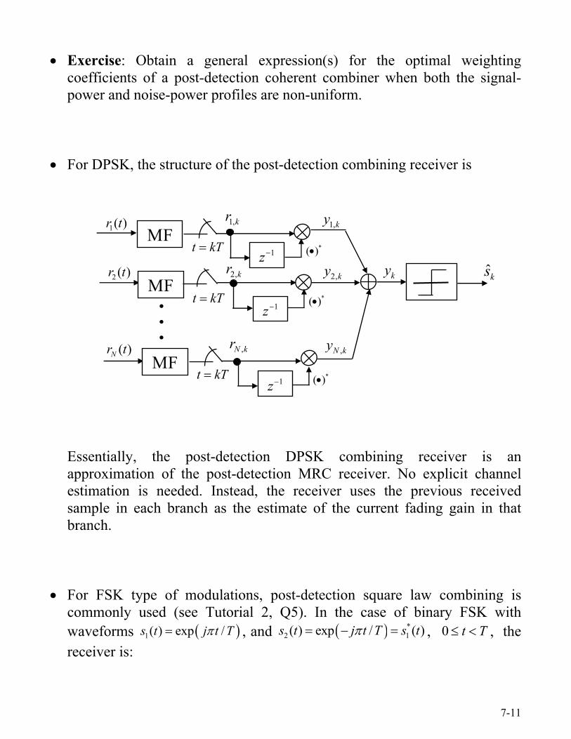
For DPSK, the structure of the post-detection combining receiver is

,N kr

2,kr

1,kr

ky

,N ky

2,ky

1,ky

•••

t kT=

t kT=

t kT=

*( )•

*( )•

*( )•

2 ( )r t

( )Nr t

1( )r tMF

ˆksMF

MF1z−

1z−

1z−

Essentially, the post-detection DPSK combining receiver is an approximation of the post-detection MRC receiver. No explicit channel estimation is needed. Instead, the receiver uses the previous received sample in each branch as the estimate of the current fading gain in that branch.

For FSK type of modulations, post-detection square law combining is commonly used (see Tutorial 2, Q5). In the case of binary FSK with waveforms (1( ) exp /s t j tπ= T , and ( ) *

2 ( ) exp / ( )1s t j t Tπ= − = s t 0 t T≤ <, , the receiver is:

7-11

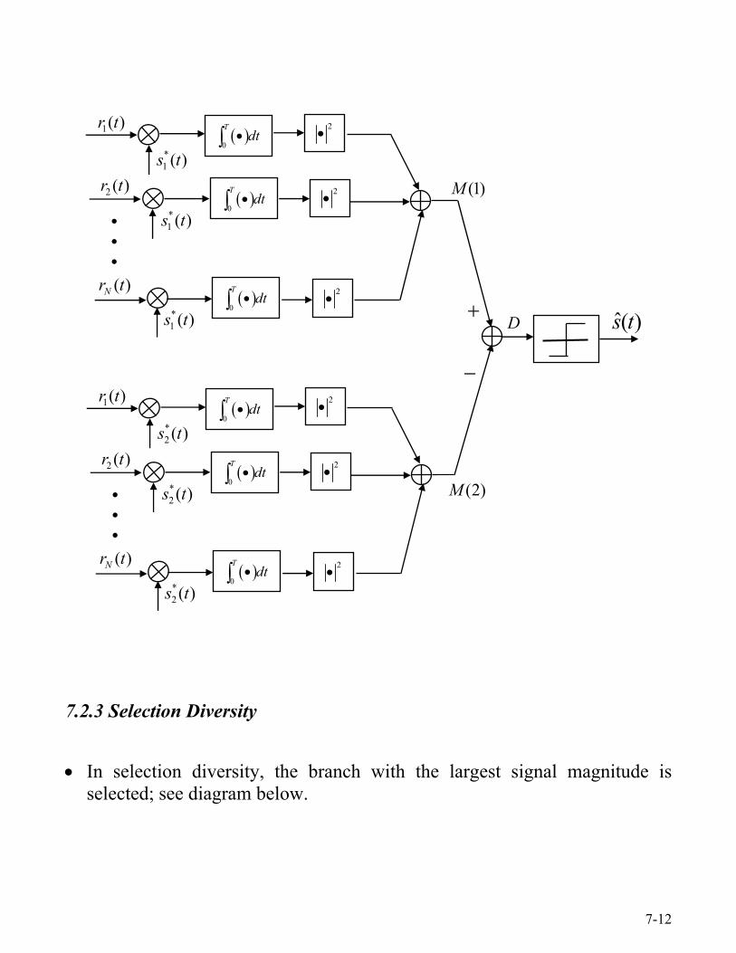
D

(1)M

−

+ ˆ( )s t

•••

*1 ( )s t

*1 ( )s t

2 ( )r t

( )Nr t

1( )r t

*1 ( )s t

2•( )0

Tdt•∫

( )0

Tdt•∫

( )0

Tdt•∫

2•

2•

•••

*2 ( )s t

*2 ( )s t

2 ( )r t

( )Nr t

1( )r t

*2 ( )s t

2•( )0

Tdt•∫

( )0

Tdt•∫

( )0

Tdt•∫

2•

2•

(2)M

7.2.3 Selection Diversity

In selection diversity, the branch with the largest signal magnitude is selected; see diagram below.

•

7-12

MIX

MIXLNA

1( )r t%IF

LO

MIXLNA

2 ( )r t%IF

LNA

( )Nr t%IF

•••

Detect.

Select Largest Magnitude

Selection is done at IF, i.e. pre-detection. Still requires a lot of parallel hardware – or at least a second rapid scanning receiver to check the unused channels. However, compared to pre-detection MRC and EGC, there is no need to perform channel tracking.

•

•

Selection can be done after detection, but not much point, since the receiver might as well just perform post-detection combining.

7-13

7.3 Performance of MRC- BPSK •

•

N

Theoretically, the BEP performance of pre-detection and post-detection MRC are identical, since both assume ideal channel estimation. Consequently, we focus on post-detection MRC in the analysis.

When noises in different branches are iid, the optimal MRC receiver is

,N kr

2,kr

1,kr

ky

,N ky

2,ky

1,ky

t kT=

t kT=

t kT=

ˆks2 ( )r t

( )Nr t

1( )r t

*,N kg

*2,kg

*1,kg

•••

MF

MF

MF

Note the following :

- , is the k-th received sample in the m-th branch.

, , , , 1, 2, ,m k k m k m kr s g n m= + = L

- { }1ks ∈ ± is the k-th transmitted BPSK symbol in all the branches. - Each is a zero mean complex Gaussian random variable with

variance ,m kg

2gσ and the different ’s are independent. ,m kg

7-14

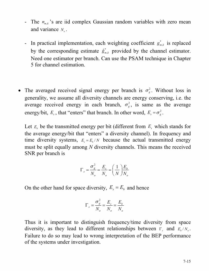
- The ’s are iid complex Gaussian random variables with zero mean and variance .

,m kn

oN

- In practical implementation, each weighting coefficient is replaced

by the corresponding estimate provided by the channel estimator. Need one estimator per branch. Can use the PSAM technique in Chapter 5 for channel estimation.

*,m kg

*,ˆm kg

The averaged received signal energy per branch is 2gσ . Without loss in

generality, we assume all diversity channels are energy conserving, i.e. the average received energy in each branch, 2

gσ , is same as the average energy/bit, sE , that “enters” that branch. In other word, 2

s gE σ= .

•

Let be the transmitted energy per bit (different from bE sE which stands for the average energy/bit that “enters” a diversity channel). In frequency and time diversity systems, /s bE E N= because the actual transmitted energy must be split equally among N diversity channels. This means the received SNR per branch is

2 1g s b

so o o

E EN N N Nσ Γ = = =

On the other hand for space diversity, s bE E= and hence

2g s b

so o o

E EN N Nσ

Γ = = =

Thus it is important to distinguish frequency/time diversity from space diversity, as they lead to different relationships between sΓ and . Failure to do so may lead to wrong interpretation of the BEP performance of the systems under investigation.

/b oE N

7-15

The combiner output can be written as •

( )* *, , , , ,

1 1

2 *, , ,

1 1

N N

k m k m k m k k m km m

N N

m k k m k m km m

k

y r g g s n g

g s g n

zs n

= =

= =

= = +

= +

= +

∑ ∑

∑ ∑

m k

where 2

,1 1

N N

m k mm m

z g z= =

= =∑ ∑

2

,m m kz g= and

*, ,

1

N

m k m km

n g n=

= ∑

If is positive, then the receiver decides that , else it decides that .

Re{ }ky

ks = −

1ks = +

1 We will use TWO different approaches to analyze the BEP performance of the MRC system. Without loss in generality, we set 1ks = . This means an error is made when

is less than zero. Re{ }ky

7.3.1 The Conditional Error Probability Approach

7-16

Consider the noise term *, ,1

Nm k m km

n g n=

= ∑ . Conditioned on the fading gains ’s, is a zero mean complex Gaussian random variable with a variance

of ,m kg n

•

22 * * *1 1 1

, , , , , , , ,2 2 21 1 1 1

2

,1

N N N N

n m k m k j k j k m k j k m k j km j m j

N

o m km

o

E n E g n g n E g g n n

N g

N z

σ= = = =

=

= = = *

=

=

∑ ∑ ∑∑

∑

•

Conditioned on and 1ks = 1 2( , , , )Nz z z=Z K , the probability that is less than zero is

ky

1( )N

mme

n o

zz zP Q Q QN Nσ

= = = =

∑Zo

,

where the term inside the Q-function is the instantaneous SNR at the combiner output. Since (see Section 4.1)

/ oz N

/ 2 2

20

1( ) exp2sin ( )

xQ x dπ

θπ θ

= −

∫ ,

we can express the conditional error probability as

/ 2

210

/ 2

210

1 1( ) exp2 sin ( )

1 exp2 sin ( )

N

e mmo

Nm

m o

P zN

z dN

π

π

dθπ θ

θπ θ

=

=

= −

= −

∑∫

∏∫

Z

7-17

The product form of the integrand makes it quite easy to obtain the unconditional error probability (see below). This is one of the nice features provided by the alternative form of the Q-function. The unconditional error probability is ( ) ( )e e zP P p d= ∫ Z Z Z , where is

the joint pdf of the

( )zp Z2

,m m kz g=

mz

’s. Since the fading gains in the different diversity branches are independent, the ’s are also independent. This means the joint pdf of the ’s is simply the product of the pdf’s of the individual ’s. As shown in Section 4.1, the pdf’s of the ’s are

mz

zmz m

•

2 2

1( ) exp2 2m

mz m

g g

zp zσ σ

= −

(this stems from the fact that each complex gain is zero mean complex Gaussian with a variance of

,m kg2gσ ). Subsequently,

2 21 1

1( ) ( ) exp2 2m

NN N

mz z m

m mg g

zp p zσ σ= =

= = −

∏ ∏Z

and the unconditional error probability becomes

1 0

0

/ 2

12 2 21 10 0

2 2 2

( ) ( )

1 1 exp exp2 2 2 sin ( )

1 1 exp exp2 2 2 sin ( )

N

m

e e z

NN N

m mN

m mg g oz z

m mm

m g g oz

P P p d

z z d dz dzN

z z dzN

π

θ

θσ σ π θ

π σ σ θ

=

=

∞ ∞

= == =

∞

=

= − −

= − −

∫

∏ ∏∫ ∫ ∫

∫

Z Z Z

L L

/ 2

10

/ 2

20

1 1sin

N

Ns

d

d

π

θ

π

θ

θ

θπ θ

==

−

=

Γ = +

∏∫

∫

7-18

where 2 /s g NσΓ = o

•

•

•

is the branch SNR. Except for small diversity order N, it is cumbersome to evaluate the above integral analytically. However, evaluating it numerically is very straight forward.

It is also relatively straight forward to generalize the above error probability expression to the case of a non-uniform signal-power profile (i.e. when the average received signal energy in the different branches are not identical).

When the branch SNR, sΓ , is fixed, the integrand decreases monotonically as N increases. In other word, the error probability for space diversity can be made, in theory, arbitrarily small.

For large branch SNR, i.e. 21 sins θΓ >> > , then •

/ 2 / 222

0 0

1 sin 1 1 sin

1 1 1 3 (2 1) 2 2 4 (2 )

2 11 1 4

NN

e Ns s

Ns

N Ns

P d

NN

NN

π π

θ θ

θ dθ θ θπ π= =

≈ = Γ Γ

−=Γ

− = Γ

∫ ∫L

L

where !!( )!

a ab b a b

= − . This equation is the same as [Proakis, Eqn. 4-4-18]

and it clearly indicates that the error probability decreases at a rate equal to the inverse N-th power of the branch SNR.

7-19

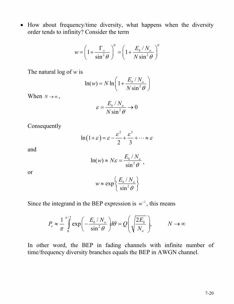
How about frequency/time diversity, what happens when the diversity order tends to infinity? Consider the term

•

2 2

/1 1sin sin

N Ns bE Nw

No

θ θΓ = + = +

The natural log of w is

2

/ln( ) ln 1sinb oE Nw N

N θ = +

When , N →∞

2

/ 0sinb oE N

Nε

θ= →

Consequently

( )2 3

ln 12 3ε εε ε ε+ = − + + ≈L

and

2

/ln( )sin

b oE Nw Nεθ

≈ = ,

or

2

/expsin

b oE Nwθ

≈

Since the integrand in the BEP expression is 1w− , this means

/ 2

20

/ 21 exp , sin

b o be

o

E N EP d QN

π

θπ θ

≈ − = ∫ N →∞

In other word, the BEP in fading channels with infinite number of time/frequency diversity branches equals the BEP in AWGN channel.

7-20

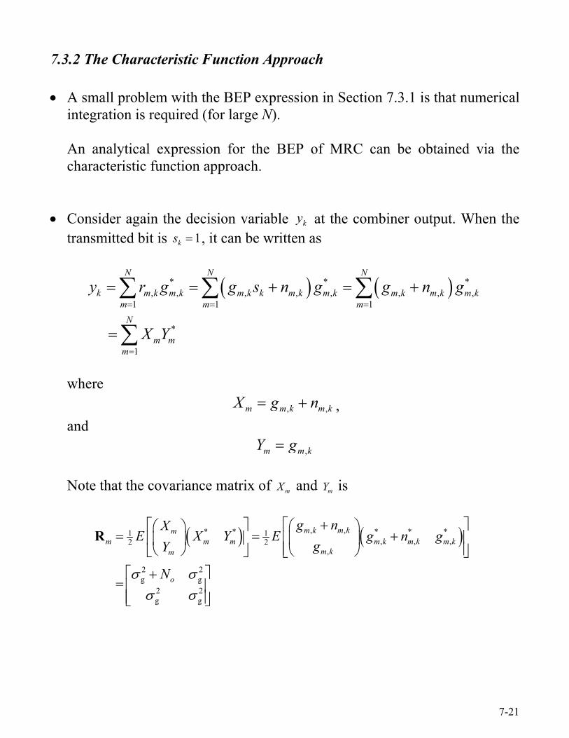
7.3.2 The Characteristic Function Approach •

•

) *g

,k

A small problem with the BEP expression in Section 7.3.1 is that numerical integration is required (for large N).

An analytical expression for the BEP of MRC can be obtained via the characteristic function approach. Consider again the decision variable at the combiner output. When the transmitted bit is , it can be written as

ky1ks =

( ) (* *, , , , , , , ,

1 1 1

*

1

N N N

k m k m k m k k m k m k m k m k m km m m

N

m mm

y r g g s n g g n

X Y

= = =

=

= = + = +

=

∑ ∑ ∑

∑

where

,m m k mX g n= + , and

,m mY kg= Note that the covariance matrix of mX and Y is m

( ) ( ), ,* * * * *1 1, , ,2 2

,

2 2g g

2 2g g

=

m k m kmm m m m k m k

m km

o

g nXE X Y E g n g

gY

Nσ σσ σ

m k

+ = = +

+

R

7-21

•

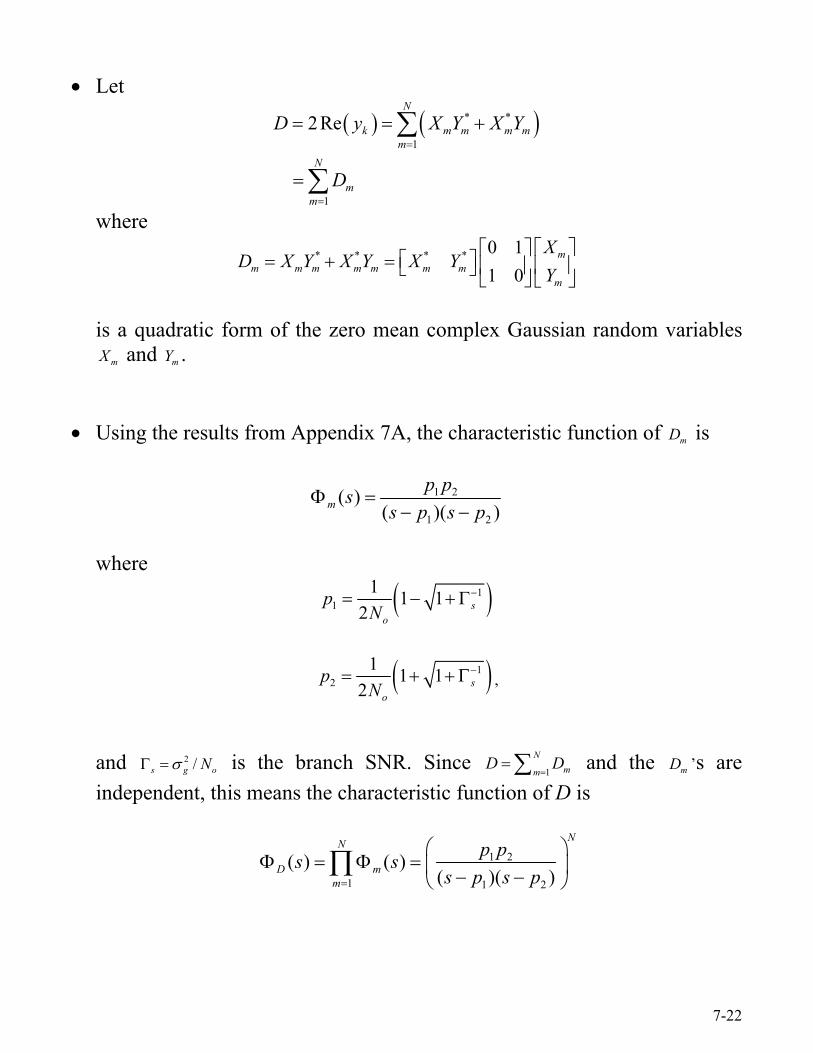
m m

Let

( ) ( )* *

1

1

2Re

N

k m mm

N

mm

D y X Y X

D

=

=

= = +

=

∑

∑

Y

where * * * * 0 1

1 0m

m m m m m m mm

XD X Y X Y X Y

Y = + =

is a quadratic form of the zero mean complex Gaussian random variables

mX and Y . m

Using the results from Appendix 7A, the characteristic function of is mD•

1 2

1 2

( )( )(m

p ps)s p s p

Φ =− −

where

( )11

1 1 12 s

o

pN

−= − + Γ

( )12

1 1 12 s

o

pN

−= + + Γ ,

and 2 /s g NσΓ = o D is the branch SNR. Since 1

Nmm

D=

=∑ and the ’s are independent, this means the characteristic function of D is

mD

1 2

1 1 2

( ) ( )( )( )

NN

D mm

p ps ss p s p=

Φ = Φ = − −

∏

7-22

Since , the receiver makes a wrong a decision if . This error probability can be determined by first taking the inverse Laplace transform of

1ks =

( )

0D <

D sΦ to obtain the pdf of D, and then integrating this pdf from D = −∞ to . From Appendix 7A, 0D =

•

[ ]1

1 2

01 2 2 1

1Pr 0

N jN

j

N jp pDjp p p p

−

=

+ − < = − −

∑ .

Consequently,

[ ]1

1 10

11 1 1 1Pr 0 1 12 21 1

N jN

ejs s

N jP D

j

−

− −=

+ − = < = − + + Γ + Γ ∑

•

Check: For N=1 (no diversity), the result is identical to the one in Section 4.1. Also the result is identical to Eqn. 14-4-5 in [Proakis].

The figures below show the BEP of MRC-BPSK with finite diversity order. Both space and frequency/time diversity techniques are considered. Note: - The BEP of coherent BPSK in AWGN channel is ( )2 /b oNQ E . - Asymptotic slope is ( )/ N

b oE N − as predicted in Section 7.1

- In frequency/time diversity, the split signals are combined with no lost energy.

- In space diversity, additional power from each branch saves tens of dB!

7-23

0 5 10 15 20 25 3010

-8

10-6

10-4

10-2

100

Eb/No (dB)

BE

P o

f MR

C-B

PS

K

BEP of MRC-BPSK with frequency/time diversity. The various curves (from top) are for diversity orders 1, 2, 4, 8, 16, and the AWGN channel.

0 5 10 15 20 25 3010

-8

10-6

10-4

10-2

100

Eb/No (dB)

BE

P

BEP of MRC-BPSK with space diversity. The color curves (from top) are for diversity orders 1, 2, 4, 8, 16. The black curve is for the AWGN channel.

7-24

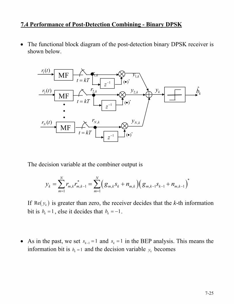
7.4 Performance of Post-Detection Combining - Binary DPSK

•

)

The functional block diagram of the post-detection binary DPSK receiver is shown below.

•••

t kT=

t kT=

t kT=

2 ( )r t

( )Nr t

1( )r tMF

MF

MF

The decision variable at t

*

, , 11

N

k m k m km

y r r −=

= =∑

If is greater than zbit is , else it decide

(Re ky

kb =1

As in the past, we set 1ks −

information bit is b an1k =

•

1,kr

,N kr

2,kr

(•

( )•

*( )•

1z−

1z−

1z−

he combiner out

( ,1

N

m k km

g s n=

+∑

ero, the receives that 1kb = − .

and 1= 1ks = ind the decision v

)− −

1,ky

ky

,N ky

2,ky

*)

*

k̂b

put is

)( *, , 1 1 , 1m k m k k m kg s n− +

r decides that the k-th information

the BEP analysis. This means the ariable becomes ky

7-25

( )( *, , , 1 , 1

1

*

1

N

k m k m k m k m km

N

m mm

y g n g n

X Y

− −=

=

= + +

=

∑

∑

)

k

where

, ,m m k mX g n= + and

, 1 , 1m m k m kY g n− −= +

Using the results from Appendix 4A or Appendix 7A, the covariance matrix of each pair of mX and Y is m

( )

( )

* *12

, , * * * *, , , 1 , 1

, 1 , 1

2 2g g

2 2g g

1 2

=

mm m m

m

m k m km k m k m k m k

m k m k

o

o

XE X Y

Y

g nE g n g

g n

N JJ N

σ σσ σ

− −− −

=

+

= + + + +

R

n

+

where (2 )o dJ J f Tπ , is the zero-order Bessel function, ( )oJ • df is the maximum Doppler frequency, and 1/T is the bit rate.

•

m m

We will use the characteristic function approach to determine the BEP. Let

( ) ( )* *

1

1

2Re

N

k m mm

N

mm

D y X Y X

D

=

=

= = +

=

∑

∑

Y

7-26

where * * * * 0 1

1 0m

m m m m m m mm

XD X Y X Y X Y

Y

= + =

is a quadratic form of the zero mean complex Gaussian random variables

mX and Y . m

Using the results from Appendix 4A (or Appendix 7A), the characteristic function of is mD

•

1 2

1 2

( )( )(m

p ps)s p s p

Φ =− −

where

( )11 1

2 1 (1 )o s

pN J−

=+ + Γ

( )21 1

2 1 (1 )o s

pN J

=+ − Γ

and sΓ is the branch SNR. Since

1

Nmm

D=

= D∑ and the ’s are independent, this means the characteristic function of D is

mD

1 2

1 1 2

( ) ( )( )( )

NN

D mm

p ps ss p s p=

Φ = Φ = − −

∏

Given that the information bit is b 1k = , the receiver makes a wrong a decision if . From Appendix 7A, 0D <

•

7-27

[ ]1

1 2

01 2 2 1

1Pr 0

N jN

j

N jp pDjp p p p

−

=

+ − < = − −

∑ .

Substituting 1p and 2p into the above equation yields

[ ]1

1 10

11 1Pr 0 1 12 1 2 1

N jN

ejs s

N jJ JP Dj

−

− −=

+ − = < = − + + Γ + Γ

∑

•

Check: For N=1 (no diversity), the result is identical to the one in Section 4.3.1.

Results for frequency/time diversity at 0df T = and 0.03df T = are shown in the next two figures.

Note: - BEP of binary DPSK in AWGN channel is /1

2bE Noe− .

- Diversity also improves the error floor.

- Curves for large N are poorer than smaller N at low SNR. The reason:

splitting the power makes SNR per branch very low. This means the reference signals provided by the previous received samples are too noisy to allow a good coherent combination. We don’t recover all the transmitted power.

7-28

0 5 10 15 20 25 3010

-8

10-6

10-4

10-2

100

Eb/No (dB)

BE

P

BEP of binary DPSK combining with time/frequency diversity. The color curves (from top) are for diversity orders 1, 2, 4, 8, 16. The black curve is for the AWGN channel. The fade rate is . 0df T =

0 5 10 15 20 25 3010

-8

10-6

10-4

10-2

100

Eb/No (dB)

BE

P

BEP of binary DPSK combining with time/frequency diversity. The color curves (from top) are for diversity orders 1, 2, 4, 8, 16. The black curve is for the AWGN channel. The fade rate is . 0.03df T =

7-29

Results for space diversity at 0df T = are shown below. As opposed to frequency/time diversity, the different curves do not cross over because the extra power gives a big boost.

•

0 5 10 15 20 25 3010

-8

10-6

10-4

10-2

100

Eb/No (dB)

BE

P

BEP of binary DPSK combining with space diversity. The color curves (from top) are for diversity orders 1, 2, 4, 8, 16. The black curve is for the AWGN channel. The fade rate is 0df T = .

7.5 Space-Time Code – A Transmit Diversity Technique References [1] S. Alamouti, “A simple transmit diversity technique for wireless communications,”

IEEE J. Select. Areas Commun., vol. 16, pp. 1451–1458, Oct. 1998. [2] V. Tarokh, N. Seshadri and A. R. Calderbank, “Space-time codes for high data rate

wireless communication: Performance criterion and code construction,” IEEE Trans. Inform. Theory, vol. 44, pp. 744–765, Mar. 1998.

[3] V. Tarokh, H. Jafarkhani and A. R. Calderbank, “Space-time block codes from

orthogonal designs” IEEE Trans. Inform. Theory, vol. 45, pp. 1456–1467, July 1999.

7-30

[4] V. Tarokh and H. Jafarkhani, “A differential detection scheme for transmit diversity,” IEEE J. Select. Areas Commun., vol. 18, pp. 1169–1174, July 2000.

[5] B. Hughes, “Differential space-time modulation,” IEEE Trans. Inform. Theory, vol.

46, pp. 2567–2578, Nov. 2000. • We considered earlier two transmit diversity techniques o frequency diversity - repeating the information in frequency domain. o time diversity – repeating the information in time.

• Another possibility is to repeat the same information using multiple transmit antennas.

• We focus on space-time (ST) codes with two transmit antennas [1]. For

convenience, we assume only one receive antenna. • The k-th transmitted symbols from the Antenna 1 and Antenna 2 are

denoted by 1,ks and 2,ks respectively, where each , is a MPSK symbol from the signal set

, , 1,2i ks i =

{ }2 / 0,1, , 1j m MS e m Mπ= = −K .

These symbols are generated at a rate of 1/ at each antenna. T

7-31

• The following encoding rules are proposed by Alamouti [1]: o The time-axis is divided into ST encoding interval of width T 2s T= . In

the m-th encoding interval, the symbols transmitted by Antenna 1 and Antenna 2 are and ( )1,2 1,2 1,m ms s + ( )2,2 2,2 1,m ms s + .

o The first symbols in each interval, 1,2 2,2 and m ms s , are chosen randomly

(and independently) from the signal set S (for coherent codes only). o The second symbols must satisfy:

*

1,2 1 2,2

*2,2 1 1,2

,

.m m

m m

s s

s s+

+

= −

= +

• The 4 MPSK symbols transmitted by the two antennas in the m-th interval can be conveniently arranged into the ST symbol matrix

1,2 2,21,2 2,2* *2,2 1,21,2 1 2,2 1

m mm mm

m mm m

s ss ss ss s+ +

= = −

s .

An interesting property of this matrix is that

†22m m =s s I

for any 1,2ms and 2,2ms , where is an identity matrix of size 2. 2I We will call the coding structure an Alamouti ST structure.

7-32

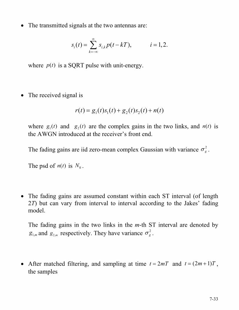
• The transmitted signals at the two antennas are:

,( ) ( ), 1,2.i i kk

s t s p t kT i∞

=−∞

= − =∑

where ( )p t is a SQRT pulse with unit-energy.

• The received signal is

1 1 2 2( ) ( ) ( ) ( ) ( ) ( )r t g t s t g t s t n t= + + where and are the complex gains in the two links, and is the AWGN introduced at the receiver’s front end.

1( )g t 2 ( )g t ( )n t

The fading gains are iid zero-mean complex Gaussian with variance 2

gσ . The psd of is . ( )n t 0N

• The fading gains are assumed constant within each ST interval (of length 2T) but can vary from interval to interval according to the Jakes’ fading model.

The fading gains in the two links in the m-th ST interval are denoted by

and 1,mg 2,mg respectively. They have variance 2gσ .

• After matched filtering, and sampling at time 2t mT= and ,

the samples (2 1)t m= + T

7-33

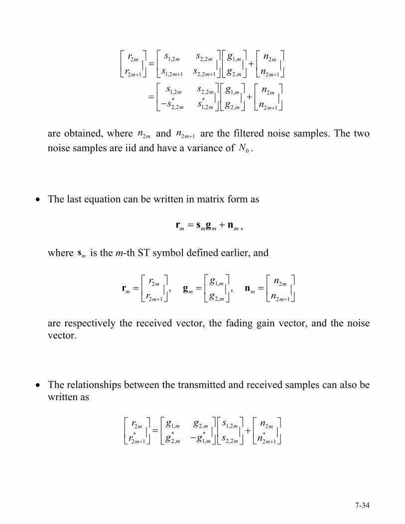
1,2 2,2 1,2 2

1,2 1 2,2 1 2,2 1 2 1

1,2 2,2 1, 2* *2,2 1,2 2, 2 1

m m mm m

m m mm m

m m m m

m m m m

s s gr ns s gr n

s s g ns s g n

+ ++ +

+

= +

= + −

are obtained, where and 2mn 2 1mn + are the filtered noise samples. The two noise samples are iid and have a variance of . 0N

• The last equation can be written in matrix form as

m m m m= +r s g n ,

where is the m-th ST symbol defined earlier, and ms

1,2 2

2,2 1 2 1

, , mm mm m m

mm m

gr ngr n+ +

= = =

r g n

are respectively the received vector, the fading gain vector, and the noise vector.

• The relationships between the transmitted and received samples can also be written as

1, 2, 1,22 2* ** *2, 1, 2,22 1 2 1

m m mm m

m m mm m

g g sr ng g sr n+ +

= + −

7-34

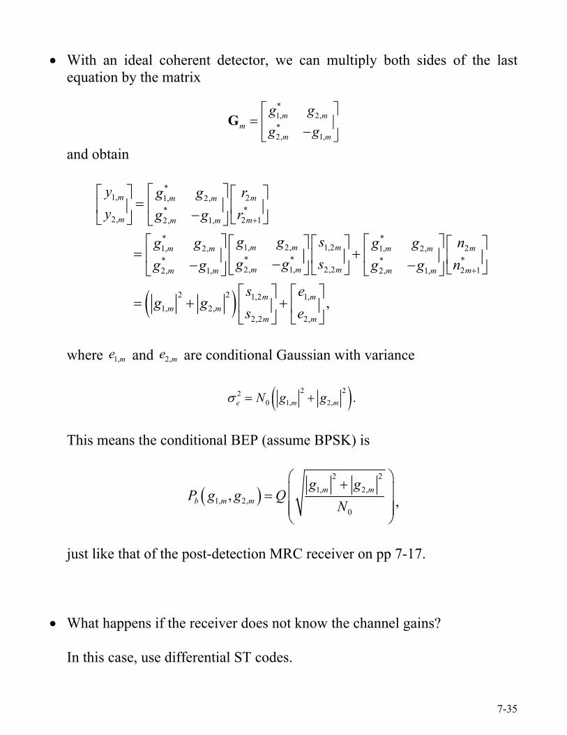
• With an ideal coherent detector, we can multiply both sides of the last equation by the matrix

*1, 2,*2, 1,

m mm

m m

g gg g

= − G

and obtain

( )

*1, 21, 2,

**2, 2 12, 1,

* *1, 2, 1,2 21, 2, 1, 2,* * ** *2, 1, 2,2 2 12, 1, 2, 1,

2 2 1,21, 2,

2

m mm m

m mm m

m m m mm m m m

m m m mm m m m

mm m

y rg gy rg g

g g s ng g g gg g s ng g g g

sg g

s

+

+

= −

= + −− −

= + 1,

,2 2,

,m

m m

ee

+

where and are conditional Gaussian with variance 1,me 2,me

( )2 220 1, 2, .e mN g gσ = + m

This means the conditional BEP (assume BPSK) is

( )2 2

1, 2,1, 2,

0

, m mb m m

g gP g g Q

N

+ =

,

just like that of the post-detection MRC receiver on pp 7-17.

• What happens if the receiver does not know the channel gains?

In this case, use differential ST codes.

7-35

• In a differential ST coding system, the data ST symbol

1, 2,* *2, 1,

m mm

m m

b bb b

= −

b

is differentially encoded into the transmitted ST symbol according to

1m m m−=s b s ,

where (and thus ) has an Alamouti structure. 1m−s ms

• Exercise: Show that if A and B are two 2 by 2 matrices with an Alamouti structure, then their product AB also has an Alamouti structure.

• Example: Full rate differential ST-BPSK code o The data ST symbols are from the set

1 2 3 4

1 0 1 0 0 1 0 1, , ,

0 1 0 1 1 0 1 0bS + − − +

= = = = = + − + − B B B B

while the transmitted ST symbols are from the set

1 2 3 4

1 1 1 1 1 1 1 1, , ,

1 1 1 1 1 1 1 1aS + + − − + − − +

= = = = = − + + − + + − − A A A A .

The detail encoding rule, with bit-assignment, are given in the table below

7-36

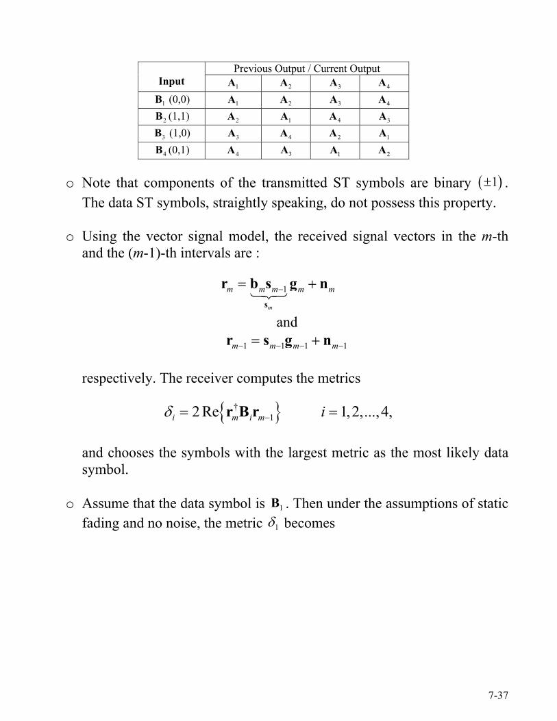
Previous Output / Current Output

Input 1A 2A 3A 4A

1B (0,0) 1A 2A 3A 4A

2B (1,1) 2A 1A 4A 3A

3B (1,0) 3A 4A 2A 1A

4B (0,1) 4A 3A 1A 2A

o Note that components of the transmitted ST symbols are binary ( )1± . The data ST symbols, straightly speaking, do not possess this property.

o Using the vector signal model, the received signal vectors in the m-th

and the (m-1)-th intervals are :

1

m

m m m m− m= +s

r b s g n123

and 1 1 1m m m m 1− − − −= +r s g n

respectively. The receiver computes the metrics

{ }†12 Re 1,2,...,4,i m i m iδ −= =r B r

and chooses the symbols with the largest metric as the most likely data symbol.

o Assume that the data symbol is . Then under the assumptions of static

fading and no noise, the metric 1B

1δ becomes

7-37

( ) ( ){ }( )( ){ }{ }

( )

† † †1 1 1 1

† †1 1

†

2 21, 1,

2 Re

2 Re

4 Re

4

m m m m

m m m m

m m

m mg g

δ − −

− −

=

=

=

= +

g s B B s g

g s s g

g g

1

2 1δ δ= − ,

3 4 10 (for any )mδ δ −= = s .

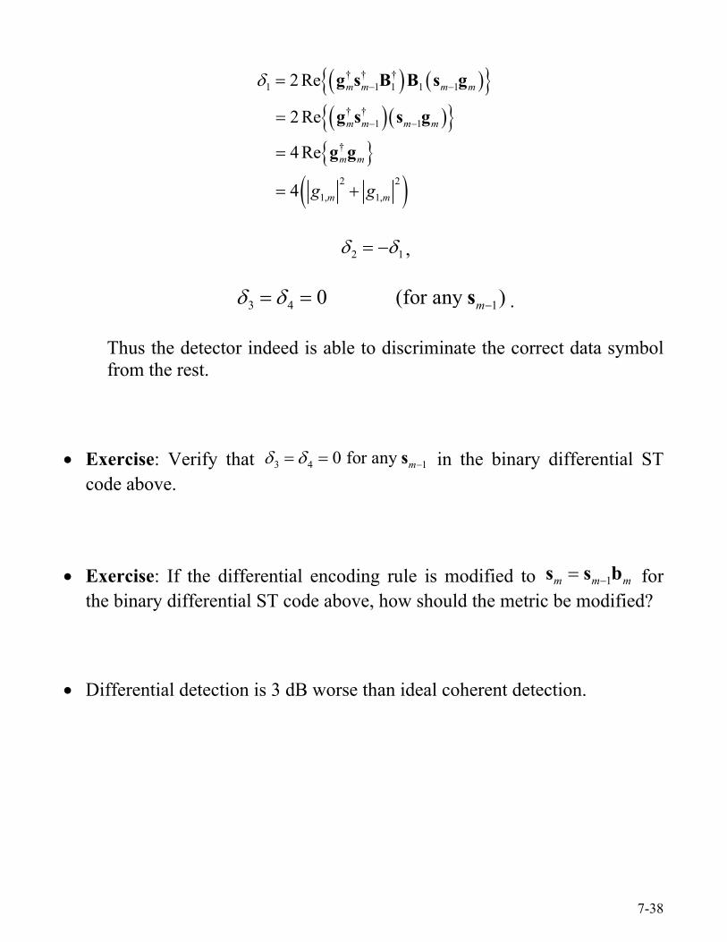
Thus the detector indeed is able to discriminate the correct data symbol from the rest.

• Exercise: Verify that 3 4 0 for any m 1δ δ −= = s in the binary differential ST

code above. • Exercise: If the differential encoding rule is modified to for

the binary differential ST code above, how should the metric be modified? 1m m−=s s bm

• Differential detection is 3 dB worse than ideal coherent detection.

7-38

Appendix 7A: Quadratic Form of Diversity Systems • As shown in Section 2.3 and Appendix 2A, the probability density function

(pdf) of a set of zero mean correlated complex Gaussian random variables

1 2( , , , )tKz z z=z L

is

( )† 112

1( ) exp(2 )z Kpπ

−= −z zR

R z

where †1

2 E = R z z is the covariance matrix of z. In addition, the characteristic function of the quadratic form

†Q = z Fz

is

( ) ( )† 1 †12

1( ) exp exp(2 )

1 2

Q Ks s d

s

π−Φ = − −

=+

∫ z R z z Fz zR

I RF

where it is understood that †=F F . As stated before, the characteristic function is the Laplace transform of the pdf.

• We are interested here in the case of 2K = , a covariance matrix of

( )1 11 12* * *11 2 12 212

2 21 22

( )z

E z zz

φ φφ φ

φ φ

= =

R = ,

and

7-39

0 11 0

=

F

As shown in Assignment 1, Q2,

1 2

1 2

1 2 1 2

1 2 1 2 1 2

( )( )( )

1 1 ( ) (

Qp ps

s p s pp p p p

)p p s p p p s p

Φ =− −

= +− − − −

where

( ) ( ) ( )( )

2 212 12 11 22 12

1 211 22 12

Re Re0

2p

φ φ φ φ φ

φ φ φ

− + − = <

− Left hand pole

( ) ( ) ( )( )

2 212 12 11 22 12

2 211 22 12

Re Re0

2p

φ φ φ φ φ

φ φ φ

+ + − = >

− right hand pole

Furthermore, the pdf of Q, which is the inverse Laplace transform of ( )Q sΦ , is

{ }1 21 2

1 2

( ) ( ) ( )p Q p QQ

p pp Q e U Q e U Qp p

= +−

−

where is the unit step function. We are often interested in evaluating the probability that Q < 0 (as in BEP analysis). In these circumstances, only the second term in the pdf is relevant. Integrating this second term from negative infinity to zero yields

( )U •

[ ] 2

01 2 1

1 2 1 2

Pr 0 p Qp p pQ e dQp p p p−∞

< = =− −∫

7-40

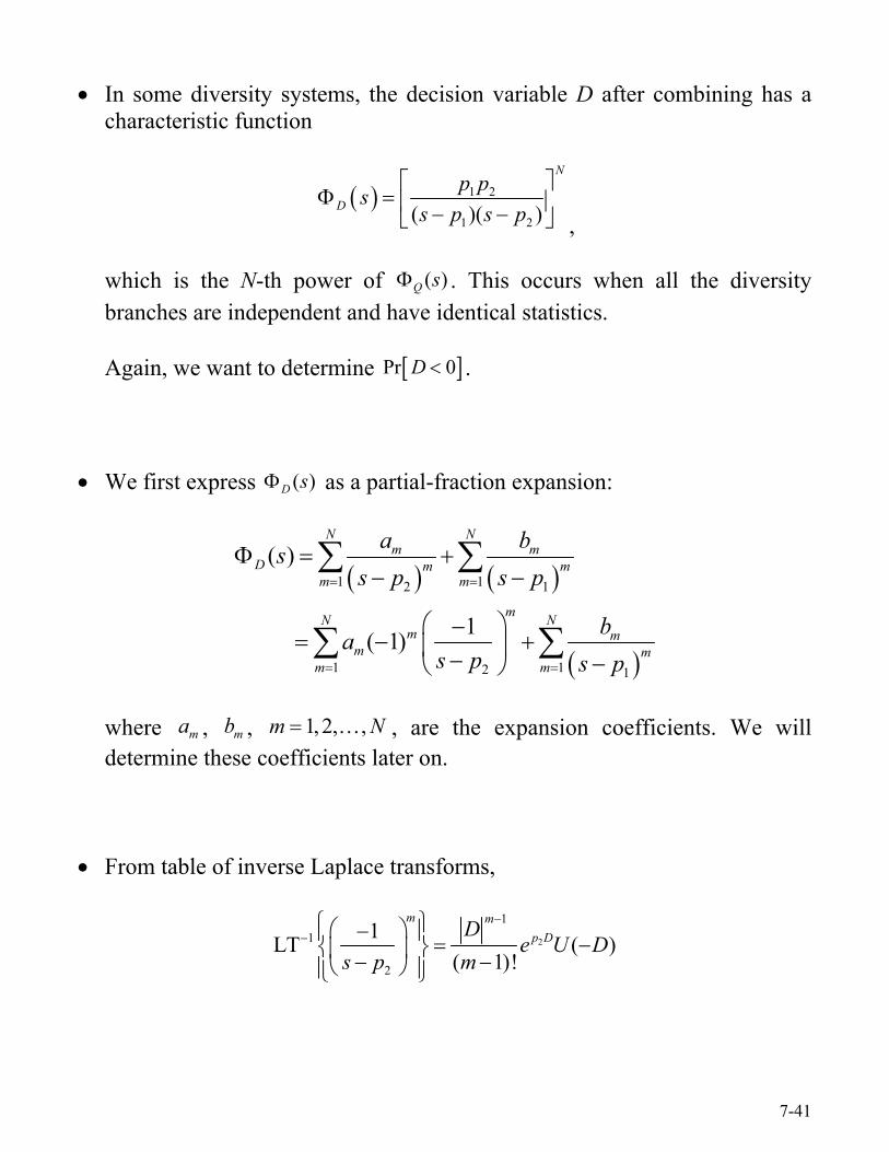
In some diversity systems, the decision variable D after combining has a characteristic function

•

( ) 1 2

1 2( )( )

N

Dp ps

s p s p

Φ = − − ,

which is the N-th power of ( )Q sΦ . This occurs when all the diversity branches are independent and have identical statistics.

Again, we want to determine [ ]Pr 0D < . We first express ( )D sΦ as a partial-fraction expansion: •

( ) ( )

( )

1 12 1

1 12 1

( )

1 ( 1)

N Nm m

D m mm m

mN Nm m

m mm m

a bss p s p

bas p s p

= =

= =

Φ = +− −

−= − + − −

∑ ∑

∑ ∑

where , , , are the expansion coefficients. We will determine these coefficients later on.

ma mb 1, 2, ,m = K N

•

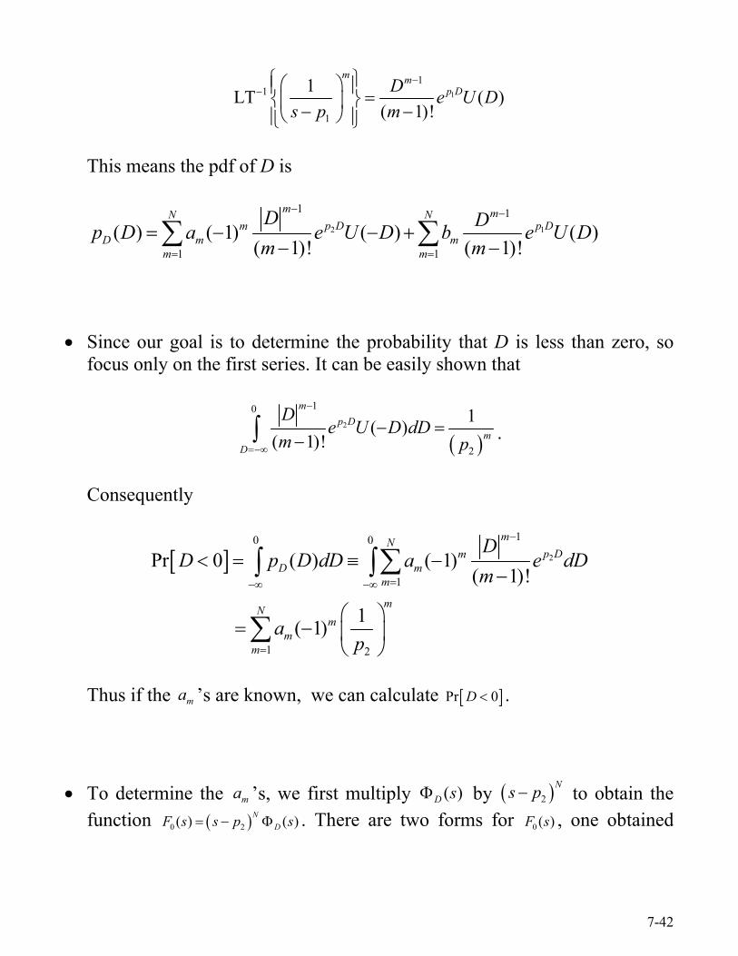
From table of inverse Laplace transforms,

2

11

2

1LT ( )( 1)!

m mp DD

e U Ds p m

−− − = − − −

7-41

1

11

1

1LT ( )( 1)!

m mp DD e U D

s p m

−− = − −

This means the pdf of D is

2 1

1 1

1 1( ) ( 1) ( ) ( )

( 1)! ( 1)!

m mN Np D p Dm

D m mm m

D Dp D a e U D b e U Dm m

− −

= =

= − − +− −∑ ∑

Since our goal is to determine the probability that D is less than zero, so focus only on the first series. It can be easily shown that

•

( )2

10

2

1( )( 1)!

mp D

mD

De U D dD

m p

−

=−∞

− =−∫ .

Consequently

[ ] 2

10 0

1

1 2

Pr 0 ( ) ( 1)( 1)!

1 ( 1)

mNp Dm

D mm

mNm

mm

DD p D dD a e dD

m

ap

−

=−∞ −∞

=

< = ≡ −−

= −

∑∫ ∫

∑

Thus if the ’s are known, we can calculate ma [ ]Pr 0D < . To determine the ’s, we first multiply ma ( )D sΦ by ( 2

N)s p−

0 ( )F s

to obtain the function . There are two forms for , one obtained ( )p0 2( ) ( )N

DF s s s= − Φ

•

7-42

from the original expression of ( )D sΦ , and a second one obtained from its partial fraction expansion:

N

N= =

N m−

1( )N sF− =

0s p=

( )j

j

dds

=

)s

( )1N j

( ) ( )1 2

0 1 21

( ) ( )( )

N Np pF s p p s p

s p−−

− 1

and

( ) ( )( )0 2 2

1 1 1

( )N N

N mm m

m m

bF s a s p s ps p= =

= − + −

− ∑ ∑

From the second expression for , we can easily deduce that 0 ( )F s

20 ( ) , N sa F s == p 2s

2

1 0 ( )s p

da F sds =

= =

p , 2

2

2

2 0 22

1 1 ( ) ( )2 2N s p

s p

da F s F sds− =

=

= =

, or

in general,

•

2

2

1 1 ( ) ( )! !

j

N j j s pj

da F s Fj ds j− == = , 0,1, , 1j N= −Ks

where

0 ( )jF s F s

is the j-th derivative of 0 ( )F s . From the first expression of , we can deduce that 0 (F•

( ) ( ) ( )1 2 1

( 1)!( )( 1)!

Nj

N jF s p p s pN

− ++ −= − −

− j

7-43

This means

( ) ( ) ( )

( ) ( )

2

( )1 2 2 1

1 22 1

2 1

1 ( )!

( 1)! 1!( 1)!

1 1

N j j s p

N j N

Nj j

a F sj

N jp p p pj N

N jp p p pjp p

− =

− +

−

=

+ −= − −

−

+ − = − − −

j

•

Finally, substituting N ja − into the expression for Pr[ 0]D < yields

1m N jN N −−

-

-

[ ]

( ) ( )

1 02 2

11 2

2 10 2 1 2

11 2

01 2 2 1

1 1Pr 0 ( 1) ( 1)

1 1 1 ( 1)

1

m N jm N j

m j

N NNj j N j

j

N N

j

D a ap p

N jp p p pjp p p

N jp pjp p p p

−−

= =

j−−− −

=

−

=

< = − = −

+ − = − − − −

+ − = − −

∑ ∑

∑

∑j

Note that the term in front of the summation operator is simply [ ]Pr 0Q < raised to the N-th power.

It should be emphasized again that the above equation is valid only for independent and identically distributed diversity branches.

7-44