Diurnal tides in mesosphere/low-thermosphere during 2002 at Wuhan (30.6°N, 114.4°E) using canonical correlation analysis

Diurnal tides in mesosphere/low-thermosphere

during 2002 at Wuhan (30.6�N, 114.4�E) usingcanonical correlation analysis

Xianghui Xue,1 Weixing Wan,2 Jiangang Xiong,2 and Xiankang Dou1

Received 8 May 2006; revised 9 September 2006; accepted 1 November 2006; published 17 March 2007.

[1] In this paper, we use canonical correlation analysis (CCA) method to investigate themesosphere/low thermosphere (MLT) diurnal tidal winds during the year 2002observed by a newly installed meteor radar at Wuhan (30.6�N, 114.4�E). In general, sixeffective diurnal tidal pairs of patterns are obtained, which represent over 90% totalvariances of the origin data set. These patterns are expected to correspond to theatmospheric oscillations within diurnal frequency band excited or modulated by differentsources, namely, the seasonal variations and the modulations by semiannual-likevariations, solar 27-day rotation and the planetary wave oscillations. Among all of thepatterns, the first pattern is the most notable, which represents �40% of total variances. Itsamplitudes show maximum values in spring and autumn as well as sudden phase transitnear equinox month, which is in line with the results obtained from traditionalharmonic analysis. The vertical wavelengths (�30 km) suggest the classic tidalmode S(1,1) is dominant, and the preceding phases (�5–6 hours) of the meridionalcomponents of the diurnal tidal wind show right-rotating circular polarization may bethe main characteristic in tidal wind.

Citation: Xue, X., W. Wan, J. Xiong, and X. Dou (2007), Diurnal tides in mesosphere/low-thermosphere during 2002 at Wuhan

(30.6�N, 114.4�E) using canonical correlation analysis, J. Geophys. Res., 112, D06104, doi:10.1029/2006JD007490.

1. Introduction

[2] Atmospheric solar tides are global-scale oscillationswith periods that are subharmonics of a solar day, which areprimarily forced by diurnal variation of heating due toabsorption of solar radiation by atmospheric water vaporand ozone. Tidal oscillations originating in the loweratmosphere and propagating upward are dominant elementsof motion systems observable at heights of MLT. Theiramplitudes are generally the largest of all the atmosphericoscillations (Gravity, Planetary and Tidal Waves), and theyplay an important role in the dynamics of MLT region asthey interact with mean flow and other waves.[3] Theoretical studies of tides in the MLT require inves-

tigation of a number of physical processes beyond thoseconsidered in classical tidal theory [Kato, 1966a, 1966b,1980], including molecular and eddy diffusion of heat andmomentum, Newtonian cooling, electrodynamic forces,radiational and chemical variations, and interactions withbackground winds and meridional temperature gradients.The early progress in tidal modeling was reviewed by Vialand Forbes [1989]. In the past two decades, some newnumerical models have been set up to investigate thedynamics process in MLT. GSWM model is one of them,

which is a 2-D linearized steady-state tidal and planetarywave model [Hagan et al., 1995, 1999, 2001]. GSWMmodel gives solutions to the linearized and extended Navier-Stokes equations for perturbation fields with characteristiczonal wave numbers and periodicities that are assumed apriori along with the zonal mean background atmosphere[Hagan and Forbes, 2002]. Another numerical model isCMAM, a 3-D nonlinear general circulation model thatextends from ground to approximately 100 km [Beagley etal., 1997; McLandress, 1997]. It includes the effects ofrealistic surface topography, planetary boundary-layereffects, a full hydrological cycle and a parameterization ofmoist convective adjustment.[4] Observations from the 1960s accompanied with very

powerful radars provide us a good opportunity to study thedynamic characteristics of tides in MLT. Atmospheric TidesMiddle Atmosphere Program (ATMAP, 1982–1988) wasput forward to research nature of atmosphere tides on aglobal international scale. It was to promote an interactionamong experimentalists, data analysis, theoreticians andmodelers with a view toward delineating the globalmorphology of tides in the middle atmosphere includingtemporal and spatial variability on various scales, and therelationships between tides, gravity waves and zonal meantemperature [Forbes, 1989]. With growth in the numbers ofboth radar and optical observational systems for MLT, itallows for more organized assessments of regional andglobal variations in the dynamical and chemical character-istics of this region [Tsuda et al., 1994, 1997; Lieberman,

JOURNAL OF GEOPHYSICAL RESEARCH, VOL. 112, D06104, doi:10.1029/2006JD007490, 2007

1University of Science and Technology of China, Hefei, China.2Institute of Geology and Geophysics, Chinese Academy of Sciences,

Beijing, China.

Copyright 2007 by the American Geophysical Union.0148-0227/07/2006JD007490

D06104 1 of 13

1997; Vincent et al., 1998; Hocke and Igarashi, 1999].PSMOS (Planetary Scale Mesopause Observing System,1998–2002) has had the major influence in this direction.Some recent papers about tidal oscillations are focused onlongitudinal and latitudinal variations in dynamic character-istics of the MLT, using radar networks in Europe, Russia,Canada and Japan [e.g., Jacobi et al., 1999; Pancheva et al.,2002; Manson et al., 2002, 2004a]. At the same time, withthe help of the scientific instruments mounted on satellites,such as HRDI/UARS, WINDII/UARS, SABER/TIMEDand TIDI/TIMED, tidal dynamics in more large scale aswell as migrating and nonmigrating tides have also beenfurther studied [e.g., Burrage et al., 1994; McLandress etal., 1994; Huang and Reber, 2003; Skinner et al., 2003;Manson et al., 2004b; Oberheide et al., 2005; Zhu et al.,2005; Wu et al., 2006]. However, there is a notable absencein African and Chinese sectors [Hocking, 1997] before 2002and only limited observations of mean winds and tides havebeen made near 30�N latitudes past and present [Zhao et al.,2005]. In such a background, wind observations of themeteor radar at Wuhan (30.6�N, 114.4�E) have been setup and obtained routine observations from 2002 [Xiong etal., 2004]; this is particularly useful for understanding thetidal variations over China.[5] In this paper, we first use the so-called canonical

correlation analysis (CCA) method to study the diurnal tides(DTs) observed at Wuhan. The meteor radar system and abrief introduction to CCA are described in section 2. Theresults from the CCA method for diurnal tides are presentedin section 3. A discussion is given in section 4 and summaryin section 5.

2. Data and Canonical Correlation AnalysisMethod

2.1. Observations and Preprocessing Data

[6] An all-sky interferometric meteor wind radar has beenin operation at Wuhan (30.6�N, 114.4�E), China, with peakpower of 7.5 kW, a duty cycle of 10% at a frequency of38.7 MHz and a height resolution of typically <2 km sinceJanuary 2002. Almost continuous observations have beencarried out from February 2002. The peak counts of meteorechoes near 91 km and almost 24-hour data coverage, whichprovides us to calculate the wind in 84- to 98-km-altituderegion.[7] The data analysis was performed by using hourly

averages of the horizontal wind of the first year observa-tions at Wuhan. The data gaps in hourly data set of a day arefilled with interpolation when the length of gap is less than9 hours. Otherwise, the following analysis does not proceedon that day. All data are passed into a band-pass filter,whose low and high cutoff frequencies are selected accord-ing to the diurnal peak in the Lomb-Scargle periodogram ofinput data, to obtain the diurnal tidal information.

2.2. A Brief Introduction to Canonical CorrelationAnalysis (CCA)

[8] Because the atmospheric oscillations of a certainfrequency may be excited or modulated by differentgeophysical sources, that is to say, when more than onetype of wave structure is present in the same frequencyband, there is a need to determine how many significant

wave structures are present and what is the relativecontribution of each wave type to the variance spectra.As for the same generating source, the correspondingoscillations should have the best correlation, in statisticalpoint of view, we can extract these oscillations apart,which are relative to an/some excited or modulatedsource(s), by studying their correlation characteristicsfrom a long-term data set. Canonical correlation analysis(CCA) is introduced for this intention.[9] CCA, which was first described by Hotelling [1936],

is a technique that is used to study the correlation structureof a pair of random vectors ~x and ~y. It is suitable foranalyzing the correlations of the wave-oscillation motionsespecially for tidal waves, which have fixed periods that aresubharmonics of a solar day. This method can help us todefine the number of significant wave oscillations present incertain frequency intervals and to separate the total oscilla-tion field into individual wave components.[10] To demonstrate the concept we let a vector ~xt

represent the m = 24 hourly (covering the characteristicperiod of tides) observed zonal wind components at time t ata given altitude, here, t = 1, 2, . . ., N (the number of theobservational day), thus the corresponding sample datamatrix can be obtained as X = {~x1, ~x2, . . ., ~xN}. The samedefinitions are carried out to~yt and Y, the only difference isthat they represent the same components (zonal) at anotheraltitude or the other components (meridional) at the samealtitude. For sake of convenience, we remove the meanvalue from~xt (~yt) and rewrite as~xt =~xt � 1

N

PNt¼1~xt (~yt =~yt �

1N

PNt¼1 ~yt).

[11] Considering a pair of sample data matrices X and Y,we try to find a pair of 24-dimensional vectors (~f x

1, ~f y1)

(subject to k~f x1k = k~f y1k = 1), such that the inner products

bx1 = hX, ~f x1i and by1 = hY, ~f y1i have maximum correlation.

The second pair of vectors (~f x2, ~f y

2) is found so that

bx2 = hX, ~f x

2i and by2 = hY, ~f y

2i are the most stronglycorrelated linear combinations of X and Y that are not corre-lated with (bx

1, by1). The derivation can now be repeated to

obtain d = min(rank(X), rank(Y)) pairs of vectors (~f xi , ~f y

i )and d corresponding pairs,

bix ¼ hX ;~f ix i ð1Þ

biy ¼ hY ;~f iy i: ð2Þ

The correlation coefficients between pairs of (bxi , by

i ) areindexed in order of decreasing values and these pairs of

(bxi , by

i ) are uncorrelated. That is, for i 6¼ j, cov(bxi , bx

j) =

cov(byi , by

j) = cov(bxi , by

j) = 0.[12] Then we can totally reconstruct X and Y through

matrices Fx and Fy:

X ¼ Fx~bx

Y ¼ Fy~by;

ð3Þ

where

~bx ¼ hX ;~f 1x i; . . . ; hX ;~f dx i� �T

¼ fTx X

D06104 XUE ET AL.: DTS IN MLT USING CCA METHOD

2 of 13

D06104

and

Fx ¼ Cov X ;Xð Þf x;

where fx is the d d matrix with vector~f xi in its ith column.

The same definition is applied to ~by and Fy. For the details,one can refer to chapter 14 in the book by von Storch andZwiers [1999]. The columns of Fx and Fy, that is, (~Fx

i , ~Fyi ),

are considered as the ith pair of the canonical correlationpatterns (CCPs), and the corresponding (bx

i , byi ) are defined

as canonical variants related with the ith canonicalcorrelation patterns.[13] Please note that equation (3) can also be written as

X ¼P

i bix~Fix

Y ¼P

i biy~Fiy:

ð4Þ

This allows us to see more clearly that equation (4) describesan expansion of X and Y with respect to their correspondingcanonical correlation patterns. It also suggests that it may bepossible to approximate X and Y by truncating thesummation in equation (4). So we define (~X i, ~Y i) as ithpair of the regressive patterns (RPs) relative to the ith CCPs,where ~X i = bx

i ~Fxi and ~Y i = by

i ~Fyi , and the regressive form of

equation (4) at truncate order k (k � d) is

~X ¼Pk

i¼1~X i

~Y ¼Pk

i¼1~Y i:

ð5Þ

[14] Total variances of X (or Y) can be represented byregressive ~X (~Y ) of the first k patterns,

R2 X ; ~X� �

¼tr cov X ;Xð Þ � cov X� ~X ;X� ~X

� �� �tr cov X ;Xð Þð Þ : ð6Þ

3. Results

3.1. CCA of Diurnal Wind Components at a Pair ofTypical Altitudes

[15] To illustrate how the CCA works, we select thefiltered zonal DT data at two typical altitudes, i.e., 86 kmand 90 km, as an example. Before analyzing the data withCCA, we use Hilbert CCA to preprocess the data, whichcombine the original times series X and its Hilbert transformXH into a new complex time series (X + iX H) [von Storchand Zwiers, 1999, chapter 16]. A generalization of thisapproach is to model not only the ’state’ X but also anindicator of its tendency dX, or we can say it allows the

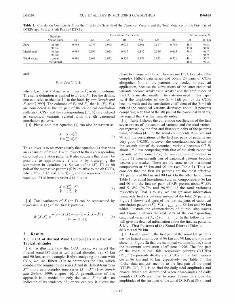
phase to change with time. Then we use CCA to analyze thecomplex Hilbert data series and obtain 24 pairs of CCPsaltogether. Not all the patterns are needed in practicalapplication, because the correlations of the latter canonicalvariants become weaker and weaker and the amplitudes ofthe CCPs are also smaller. The criterion used in this paperis: if the amplitudes of the (k + 1)th pair of the CCPsbecome weak and the correlation coefficient of the (k + 1)thpair of the canonical variants decreases about 10 percentscomparing with that of the kth pair of the canonical variants,we regard that k is the truncate order.[16] Table 1 shows the correlation coefficients of the first

seven orders of the canonical variants and the total varian-ces regressed by the first and first-sixth pairs of the patternsusing equation (4). For the zonal components at 86 km and90 km, the correlations of the first six pairs of patterns arevery good (>0.80); however, the correlation coefficient ofthe seventh pair of the canonical variants becomes 0.719,about 12% less comparing with that of the sixth canonicalvariants, at the same time, the amplitudes (not shown inFigure 1) from seventh pair of canonical patterns becomeweaker and weaker. These are the same to the meridionalcomponents at 86 km and 90 km (see Table 1). Thus weconsider that the first six patterns are the most effectiveDT patterns at 86 km and 90 km. On the other hand, fromTable 1, for zonal (meridional) diurnal components at 86 kmand 90 km, the first six pairs of RPs present about 91.8%and 91.8% (96.7% and 96.9%) of the total variancesrespectively. That is to say, we can get most informationusing only first six patterns instead of the total 24 patterns.Figure 1 shows real parts of the first six pairs of canonicalcorrelation patterns (~Fx

i , ~Fyi )i = 1,2,. . .,6 at 86 km and 90 km

which illustrate the characteristics of diurnal sine wavesand Figure 2 shows the real parts of the correspondingcanonical variants (bx

i , byi )i = 1, 2, . . ., 6. In the following, we

will give the detailed information about the first six patterns.3.1.1. First Patterns of the Zonal Diurnal Tides at86 km and 90 km[17] From Figure 1, the first pair of the zonal DT patterns

has the largest amplitudes at 86 km and 90 km, and it is alsoshown in Figure 2a that the canonical variants (bx

1, by1) have

the maximum correlation coefficient 0.996. The first pairof the zonal diurnal tidal regressive patterns (DTRPs)(~X 1, ~Y 1) represents 46.4% and 37.0% of the total varian-ces at 86 km and 90 km respectively (see Table 1). Thefurther data analysis method to the first pair of the zonalDTRPs (~X 1, ~Y 1) is to find the daily tidal amplitudes andphases, which are determined when phase-angles of dailycomplex DTRPs are fitted to zeros. Figure 3a shows theamplitudes of the first pair of the zonal DTRPs at 86 km and

Table 1. Correlation Coefficients From the First to the Seventh of the Canonical Variants and the Total Variances of the First Pair of

DTRPs and First to Sixth Pairs of DTRPs

RandomVector Pairs

Correlation Coefficients Total Variances, %

1st 2nd 3rd 4th 5th 6th 7th 1st 1st–6th

Zonal 86 km 0.996 0.979 0.948 0.930 0.861 0.847 0.719 46.4 91.890 km 37.0 91.8

Meridional 86 km 0.999 0.990 0.924 0.917 0.887 0.856 0.665 56.8 96.790 km 53.5 96.9

Wind vector zonal 0.996 0.969 0.932 0.910 0.879 0.832 0.731 48.1 92.7meridional 48.8 91.2

D06104 XUE ET AL.: DTS IN MLT USING CCA METHOD

3 of 13

D06104

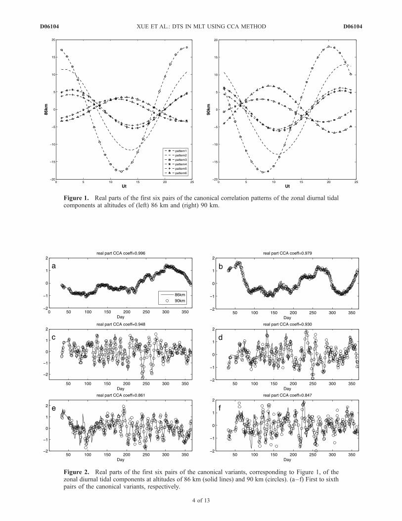
Figure 1. Real parts of the first six pairs of the canonical correlation patterns of the zonal diurnal tidalcomponents at altitudes of (left) 86 km and (right) 90 km.

Figure 2. Real parts of the first six pairs of the canonical variants, corresponding to Figure 1, of thezonal diurnal tidal components at altitudes of 86 km (solid lines) and 90 km (circles). (a–f) First to sixthpairs of the canonical variants, respectively.

D06104 XUE ET AL.: DTS IN MLT USING CCA METHOD

4 of 13

D06104

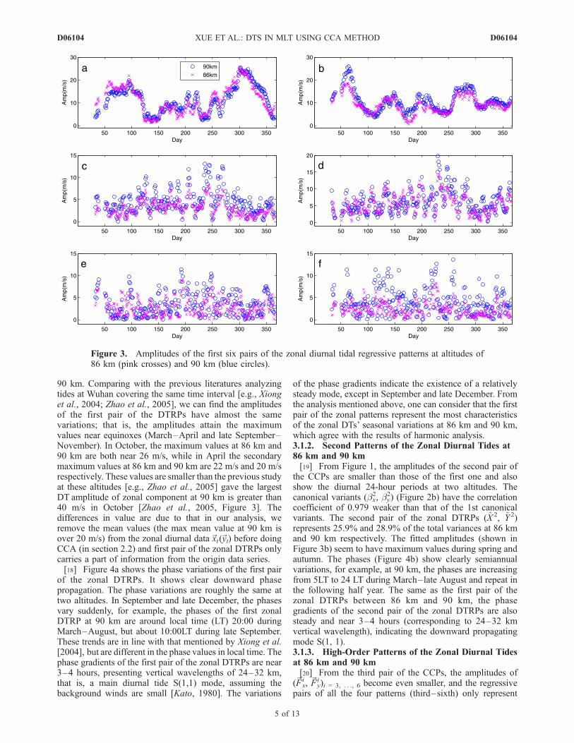
90 km. Comparing with the previous literatures analyzingtides at Wuhan covering the same time interval [e.g., Xionget al., 2004; Zhao et al., 2005], we can find the amplitudesof the first pair of the DTRPs have almost the samevariations; that is, the amplitudes attain the maximumvalues near equinoxes (March–April and late September–November). In October, the maximum values at 86 km and90 km are both near 26 m/s, while in April the secondarymaximum values at 86 km and 90 km are 22 m/s and 20 m/srespectively. These values are smaller than the previous studyat these altitudes [e.g., Zhao et al., 2005] gave the largestDT amplitude of zonal component at 90 km is greater than40 m/s in October [Zhao et al., 2005, Figure 3]. Thedifferences in value are due to that in our analysis, weremove the mean values (the max mean value at 90 km isover 20 m/s) from the zonal diurnal data~xt (~yt) before doingCCA (in section 2.2) and first pair of the zonal DTRPs onlycarries a part of information from the origin data series.[18] Figure 4a shows the phase variations of the first pair

of the zonal DTRPs. It shows clear downward phasepropagation. The phase variations are roughly the same attwo altitudes. In September and late December, the phasesvary suddenly, for example, the phases of the first zonalDTRP at 90 km are around local time (LT) 20:00 duringMarch–August, but about 10:00LT during late September.These trends are in line with that mentioned by Xiong et al.[2004], but are different in the phase values in local time. Thephase gradients of the first pair of the zonal DTRPs are near3–4 hours, presenting vertical wavelengths of 24–32 km,that is, a main diurnal tide S(1,1) mode, assuming thebackground winds are small [Kato, 1980]. The variations

of the phase gradients indicate the existence of a relativelysteady mode, except in September and late December. Fromthe analysis mentioned above, one can consider that the firstpair of the zonal patterns represent the most characteristicsof the zonal DTs’ seasonal variations at 86 km and 90 km,which agree with the results of harmonic analysis.3.1.2. Second Patterns of the Zonal Diurnal Tides at86 km and 90 km[19] From Figure 1, the amplitudes of the second pair of

the CCPs are smaller than those of the first one and alsoshow the diurnal 24-hour periods at two altitudes. Thecanonical variants (bx

2, by2) (Figure 2b) have the correlation

coefficient of 0.979 weaker than that of the 1st canonicalvariants. The second pair of the zonal DTRPs (~X 2, ~Y 2)represents 25.9% and 28.9% of the total variances at 86 kmand 90 km respectively. The fitted amplitudes (shown inFigure 3b) seem to have maximum values during spring andautumn. The phases (Figure 4b) show clearly semiannualvariations, for example, at 90 km, the phases are increasingfrom 5LT to 24 LT during March–late August and repeat inthe following half year. The same as the first pair of thezonal DTRPs between 86 km and 90 km, the phasegradients of the second pair of the zonal DTRPs are alsosteady and near 3–4 hours (corresponding to 24–32 kmvertical wavelength), indicating the downward propagatingmode S(1, 1).3.1.3. High-Order Patterns of the Zonal Diurnal Tidesat 86 km and 90 km[20] From the third pair of the CCPs, the amplitudes of

(~Fxi , ~Fy

i )i = 3, . . ., 6 become even smaller, and the regressivepairs of all the four patterns (third–sixth) only represent

Figure 3. Amplitudes of the first six pairs of the zonal diurnal tidal regressive patterns at altitudes of86 km (pink crosses) and 90 km (blue circles).

D06104 XUE ET AL.: DTS IN MLT USING CCA METHOD

5 of 13

D06104

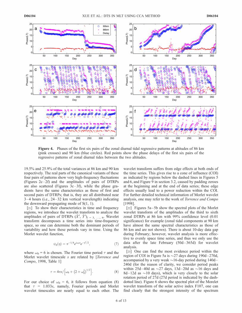
19.5% and 25.9% of the total variances at 86 km and 90 kmrespectively. The real parts of the canonical variants of thesefour pairs of patterns show very high-frequency fluctuations(Figures 2c–2f) and the amplitudes of pairs of DTRPsare also scattered (Figures 3c–3f), while the phase gra-dients have the same characteristics as those of first andsecond pairs of DTRPs; that is, they are all distributed near3–4 hours (i.e., 24–32 km vertical wavelength) indicatingthe downward propagating mode of S(1, 1).[21] To show their characteristics in time and frequency

regions, we introduce the wavelet transform to analyze theamplitudes of pairs of DTRPs (~X i, ~Y i)i = 3, . . ., 6. Wavelettransform decomposes a time series into time-frequencyspace, so one can determine both the dominant periods ofvariability and how these periods vary in time. Using theMorlet wavelet function,

y0 hð Þ ¼ p�1=4eiw0he�h2=2; ð7Þ

where w0 = 6 is chosen. The Fourier time period t and theMorlet wavelet timescale s are related by [Torrence andCompo, 1998, Table 1]

t ¼ 4ps= w0 þ 2þ w20

� �1=2h i: ð8Þ

For our choice of w0 = 6, it follows from equation (8)that t = 1.033s, namely, Fourier periods and Morletwavelet timescales are nearly equal to each other. The

wavelet transform suffers from edge effects at both ends ofthe time series. This gives rise to a cone of influence (COI)as indicated by regions below the dashed lines in Figures 5and 6, and Figure 9 in section 3.2, caused by padding zeroesat the beginning and at the end of data series; these edgeeffects usually lead to a power reduction within the COI.For further detailed technical information of Morlet waveletanalysis, one may refer to the work of Torrence and Compo[1998].[22] Figures 5a–5b show the spectral plots of the Morlet

wavelet transform of the amplitudes of the third to sixthzonal DTRPs at 86 km with 99% confidence level (0.01significance) for example (zonal tidal components at 90 kmhave almost the same spectral characteristics as those of86 km and are not shown). There is about 10-day data gapduring February; however, wavelet analysis is more effec-tive to evenly space time series, and thus we only use thedata after the late February (50d–365d) for waveletanalysis.[23] One can find the most evidence period within the

region of COI in Figure 5a is �27 days during 190d–270d,accompanied by a very weak �16-day period during 140d–240d (for the reason of clarity, we consider period peakswithin 25d–40d as �27 days, 13d–20d as �16 days and8d–12d as �10 days), which is very closely to the solarrotation period of 27d (27d period is indicated by the dash-dotted line). Figure 6 shows the spectral plot of the Moreletwavelet transform of the solar active index F107, one canfind clearly that the strongest intensity of the spectrum

Figure 4. Phases of the first six pairs of the zonal diurnal tidal regressive patterns at altitudes of 86 km(pink crosses) and 90 km (blue circles). Red points show the phase delays of the first six pairs of theregressive patterns of zonal diurnal tides between the two altitudes.

D06104 XUE ET AL.: DTS IN MLT USING CCA METHOD

6 of 13

D06104

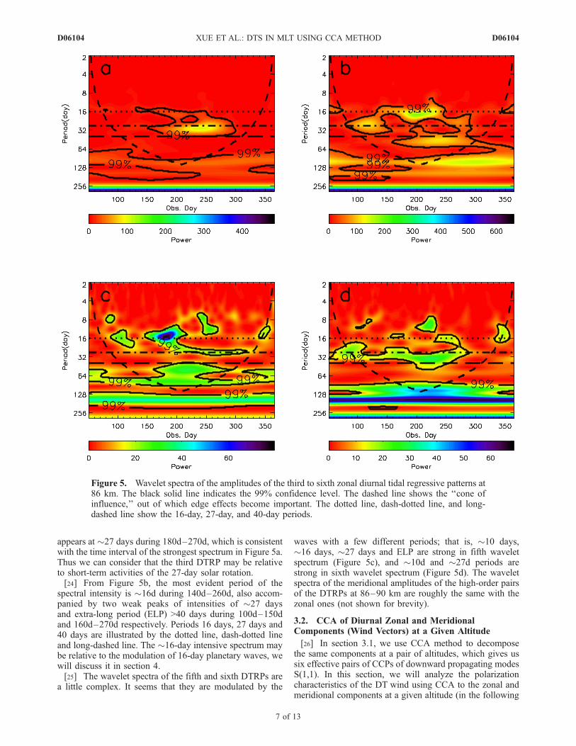
appears at �27 days during 180d–270d, which is consistentwith the time interval of the strongest spectrum in Figure 5a.Thus we can consider that the third DTRP may be relativeto short-term activities of the 27-day solar rotation.[24] From Figure 5b, the most evident period of the

spectral intensity is �16d during 140d–260d, also accom-panied by two weak peaks of intensities of �27 daysand extra-long period (ELP) >40 days during 100d–150dand 160d–270d respectively. Periods 16 days, 27 days and40 days are illustrated by the dotted line, dash-dotted lineand long-dashed line. The �16-day intensive spectrum maybe relative to the modulation of 16-day planetary waves, wewill discuss it in section 4.[25] The wavelet spectra of the fifth and sixth DTRPs are

a little complex. It seems that they are modulated by the

waves with a few different periods; that is, �10 days,�16 days, �27 days and ELP are strong in fifth waveletspectrum (Figure 5c), and �10d and �27d periods arestrong in sixth wavelet spectrum (Figure 5d). The waveletspectra of the meridional amplitudes of the high-order pairsof the DTRPs at 86–90 km are roughly the same with thezonal ones (not shown for brevity).

3.2. CCA of Diurnal Zonal and MeridionalComponents (Wind Vectors) at a Given Altitude

[26] In section 3.1, we use CCA method to decomposethe same components at a pair of altitudes, which gives ussix effective pairs of CCPs of downward propagating modesS(1,1). In this section, we will analyze the polarizationcharacteristics of the DT wind using CCA to the zonal andmeridional components at a given altitude (in the following

Figure 5. Wavelet spectra of the amplitudes of the third to sixth zonal diurnal tidal regressive patterns at86 km. The black solid line indicates the 99% confidence level. The dashed line shows the ‘‘cone ofinfluence,’’ out of which edge effects become important. The dotted line, dash-dotted line, and long-dashed line show the 16-day, 27-day, and 40-day periods.

D06104 XUE ET AL.: DTS IN MLT USING CCA METHOD

7 of 13

D06104

part we regard the zonal and meridional components pair ofDT wind as DT wind vector for short).[27] In the case of 86 km which we select as an example,

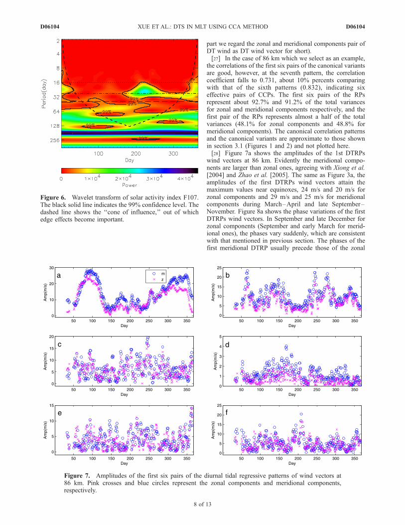
the correlations of the first six pairs of the canonical variantsare good, however, at the seventh pattern, the correlationcoefficient falls to 0.731, about 10% percents comparingwith that of the sixth patterns (0.832), indicating sixeffective pairs of CCPs. The first six pairs of the RPsrepresent about 92.7% and 91.2% of the total variancesfor zonal and meridional components respectively, and thefirst pair of the RPs represents almost a half of the totalvariances (48.1% for zonal components and 48.8% formeridional components). The canonical correlation patternsand the canonical variants are approximate to those shownin section 3.1 (Figures 1 and 2) and not plotted here.[28] Figure 7a shows the amplitudes of the 1st DTRPs

wind vectors at 86 km. Evidently the meridional compo-nents are larger than zonal ones, agreeing with Xiong et al.[2004] and Zhao et al. [2005]. The same as Figure 3a, theamplitudes of the first DTRPs wind vectors attain themaximum values near equinoxes, 24 m/s and 20 m/s forzonal components and 29 m/s and 25 m/s for meridionalcomponents during March–April and late September–November. Figure 8a shows the phase variations of the firstDTRPs wind vectors. In September and late December forzonal components (September and early March for merid-ional ones), the phases vary suddenly, which are consistentwith that mentioned in previous section. The phases of thefirst meridional DTRP usually precede those of the zonal

Figure 6. Wavelet transform of solar activity index F107.The black solid line indicates the 99% confidence level. Thedashed line shows the ‘‘cone of influence,’’ out of whichedge effects become important.

Figure 7. Amplitudes of the first six pairs of the diurnal tidal regressive patterns of wind vectors at86 km. Pink crosses and blue circles represent the zonal components and meridional components,respectively.

D06104 XUE ET AL.: DTS IN MLT USING CCA METHOD

8 of 13

D06104

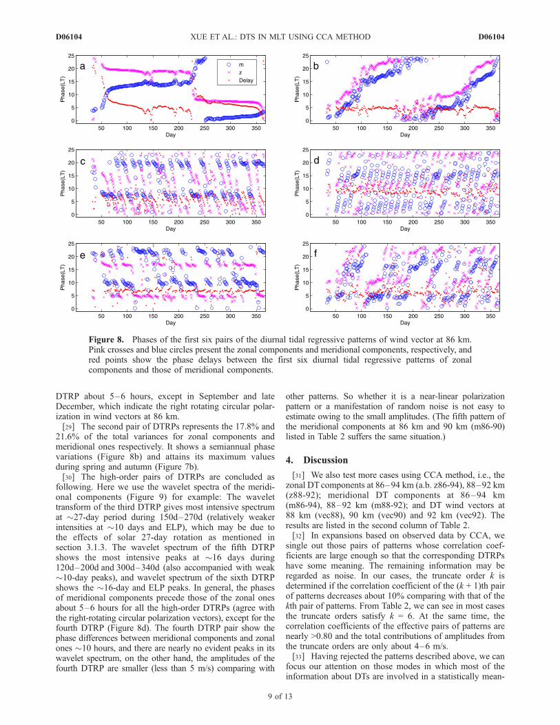
DTRP about 5–6 hours, except in September and lateDecember, which indicate the right rotating circular polar-ization in wind vectors at 86 km.[29] The second pair of DTRPs represents the 17.8% and

21.6% of the total variances for zonal components andmeridional ones respectively. It shows a semiannual phasevariations (Figure 8b) and attains its maximum valuesduring spring and autumn (Figure 7b).[30] The high-order pairs of DTRPs are concluded as

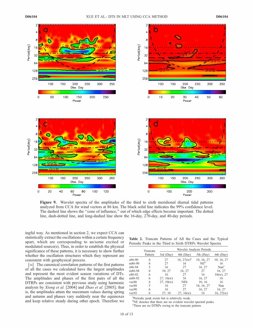
following. Here we use the wavelet spectra of the meridi-onal components (Figure 9) for example: The wavelettransform of the third DTRP gives most intensive spectrumat �27-day period during 150d–270d (relatively weakerintensities at �10 days and ELP), which may be due tothe effects of solar 27-day rotation as mentioned insection 3.1.3. The wavelet spectrum of the fifth DTRPshows the most intensive peaks at �16 days during120d–200d and 300d–340d (also accompanied with weak�10-day peaks), and wavelet spectrum of the sixth DTRPshows the �16-day and ELP peaks. In general, the phasesof meridional components precede those of the zonal onesabout 5–6 hours for all the high-order DTRPs (agree withthe right-rotating circular polarization vectors), except for thefourth DTRP (Figure 8d). The fourth DTRP pair show thephase differences between meridional components and zonalones �10 hours, and there are nearly no evident peaks in itswavelet spectrum, on the other hand, the amplitudes of thefourth DTRP are smaller (less than 5 m/s) comparing with

other patterns. So whether it is a near-linear polarizationpattern or a manifestation of random noise is not easy toestimate owing to the small amplitudes. (The fifth pattern ofthe meridional components at 86 km and 90 km (m86-90)listed in Table 2 suffers the same situation.)

4. Discussion

[31] We also test more cases using CCA method, i.e., thezonal DT components at 86–94 km (a.b. z86-94), 88–92 km(z88-92); meridional DT components at 86–94 km(m86-94), 88–92 km (m88-92); and DT wind vectors at88 km (vec88), 90 km (vec90) and 92 km (vec92). Theresults are listed in the second column of Table 2.[32] In expansions based on observed data by CCA, we

single out those pairs of patterns whose correlation coef-ficients are large enough so that the corresponding DTRPshave some meaning. The remaining information may beregarded as noise. In our cases, the truncate order k isdetermined if the correlation coefficient of the (k + 1)th pairof patterns decreases about 10% comparing with that of thekth pair of patterns. From Table 2, we can see in most casesthe truncate orders satisfy k = 6. At the same time, thecorrelation coefficients of the effective pairs of patterns arenearly >0.80 and the total contributions of amplitudes fromthe truncate orders are only about 4–6 m/s.[33] Having rejected the patterns described above, we can

focus our attention on those modes in which most of theinformation about DTs are involved in a statistically mean-

Figure 8. Phases of the first six pairs of the diurnal tidal regressive patterns of wind vector at 86 km.Pink crosses and blue circles present the zonal components and meridional components, respectively, andred points show the phase delays between the first six diurnal tidal regressive patterns of zonalcomponents and those of meridional components.

D06104 XUE ET AL.: DTS IN MLT USING CCA METHOD

9 of 13

D06104

ingful way. As mentioned in section 2, we expect CCA canstatistically extract the oscillations within a certain frequencyapart, which are corresponding to an/some excited ormodulated source(s). Thus, in order to establish the physicalsignificance of these patterns, it is necessary to show furtherwhether the oscillation structures which they represent areconsistent with geophysical process.[34] The canonical correlation patterns of the first patterns

of all the cases we calculated have the largest amplitudesand represent the most evident season variations of DTs.The amplitudes and phases of the first pairs of all theDTRPs are consistent with previous study using harmonicanalysis by Xiong et al. [2004] and Zhao et al. [2005]; thatis, the amplitudes attain the maximum values during springand autumn and phases vary suddenly near the equinoxesand keep relative steady during other epoch. Therefore we

Figure 9. Wavelet spectra of the amplitudes of the third to sixth meridional diurnal tidal patternsanalyzed from CCA for wind vectors at 86 km. The black solid line indicates the 99% confidence level.The dashed line shows the ‘‘cone of influence,’’ out of which edge effects become important. The dottedline, dash-dotted line, and long-dashed line show the 16-day, 270-day, and 40-day periods.

Table 2. Truncate Patterns of All the Cases and the Typical

Periodic Peaks in the Third to Sixth DTRPs Wavelet Spectra

TruncatePattern

Wavelet Analysis Periods

3rd (Day) 4th (Day) 5th (Day) 6th (Day)

z86-90 6 27 16, 27(w)a 10, 16, 27 10, 16, 27m86-90 6 27 16 NEb 16z86-94 5 16 27 16, 27 Nanc

m86-94 6 10, 27 16, 27 27 16, 27z88-92 6 16 27 16 10(w), 27m88-92 6 27, 16(w) 16 16, 27 16vec86 6 27, 10(w) NEb 10, 16 16vec88 5 16 27 10, 16, 27 Nanvec90 6 16 27 16, 27 16, 27vec92 6 27, 10 27, 16(w) 16 16, 27(w)

aPeriodic peak exists but is relatively weak.bNE denotes that there are no evident wavelet spectral peaks.cThere are no DTRPs owing to the truncate pattern.

D06104 XUE ET AL.: DTS IN MLT USING CCA METHOD

10 of 13

D06104

consider that from the first pattern one can get almost thesame information as the traditional method.[35] It should be noted that the second pairs of DTRPs

represent nearly 20% (or more) total variances, and thephases show clear semi-annual variations. It seems theremay be semiannual-like modulations by some atmosphericprocess. The detail of this process needs to be studiedfurther.[36] The wavelet spectra of the high-order pairs of

DTRPs have peaks at �10 days, �16 days and �27 days,especially at �16 days and �27 days. The third and fourthDTRPs can be separated as 27d-associations or 16d-associations for most cases in Table 2; on the other hand,the fifth and sixth DTRPs become complex intermixed bydifferent periodic components.[37] We consider that �16d periodic peaks may be

associated with the modulations of planetary waves(PWs) on the DTs. Lieberman et al. [2004] documentedevidence for PW-tide interactions as a source of non-migrating tides (W2) using the Nimbus 7 LIMS data.They considered that the amplitudes of W2 were en-hanced when PW penetrated to subtropical latitudes andwhen PW exhibited 16-day amplification cycles. Mansonet al. [2005] also gave an investigation of the mesosphericvariability with PW periods (2–30 days) in diurnal andsemidiurnal tides as well as total ozone and backgroundMLT winds using satellite (TOMS) and MF radar data fromCUJO network. They have shown there were some eventsthat demonstrated oscillations at PW periods (also included16-day period) in both the tides (12 hours, 24 hours) of theMLT. Jacobi et al. [1998] discovered that 16-day PWs tendto occur more frequently in winter than in summer at�95 km at Collm. Williams and Avery [1992], however,reported maximum amplitudes for 16-day PWs in summerat Poker Flat, Alaska. Luo et al. [2000] also analyzed thequasi-16-day oscillations at 60–105 km in Saskatoon,Canada, during 1980–1996 and their results show thestrong 16-day waves exist mostly in late autumn, winterand early spring. In our cases, �16-day peaks in waveletspectra occur often in summer and autumn (winter is out ofthe COI); this may be due to the fact that the backgroundzonal winds at 86 km are nearly eastward in all seasonsduring 2002 (except in April) and strongest in summer[Xiong et al., 2004], in which the 16-day PWs shouldpreferentially propagate with the evidently strong ampli-tudes [Luo, 2002]. Using the daily averaged winds ofWuhan meteor radar, Jiang et al. [2005] found therewere largest values of 16-day PWs during autumn in2002, accompanied with a second peak in summer. The�10-day spectrum peaks may be also due to the modu-lations of 10-day PWs on the DTs, but �10-day peaksare relatively weak and always mixed with other periodiccomponents (Table 2).[38] Ebel et al. [1986] investigated the response of the

middle atmosphere to solar activity oscillations of a quasi-27-day period using the data from the Saskatoon MF radarand radiosondes. They concluded that the main source ofthe 27-day oscillations induced by solar ultraviolet radiationmay be near the stratopause. Pancheva et al. [1991] haveshown some fluctuations of 24–30 days in the ionosphericabsorption of radio waves at 80- to 95-km altitudes andrelated them to variations in the neutral atmosphere with

those periods. Recently, Luo et al. [2001] first detailedassessment of the MLT 20- to 40-day oscillations andcompared these with solar parameters; they suggested thatthe oscillation could be related to the short-term solarrotation period in some way. In our analysis, we found thatthe �27-day oscillations often occur during 150d–280dwhich is very close to the peak value region of the spectrumof the solar active index F107 (Figure 6). This may be areflection of the modulations induced in tides by the solarshort-term activities.[39] Pancheva et al. [2003] assessed the variations

(3–100 days) of the semidiurnal tide observed in the MLTregion by the meteor radar in Sheffield (53�N). They haveshown that during winter the amplitude modulations ofthe semidiurnal tides have periods �10, �16, and�25–28 days, and that similar temporal variations havebeen simultaneously present in the total ozone. These resultsconfirmed the influence of the PWs together with solarshort-term activities on tides.[40] One can also find that some ELPs (usually >40 days)

appear in wavelet spectra of DTRPs (also in F107 spectrum)within the COI. Also, Pancheva et al. [2003] have illus-trated some provisional evidence for a response of thesemidiurnal tide and the total ozone to the variations inthe solar radio flux at intermediate periods of 50–80 days.These may be due to the modulations of the long-term solaractivities.[41] The vertical wavelengths and the polarization char-

acteristics of the DTs can also be attained from the CCA.For the cases of the same components (zonal or meridional)at a pair of altitudes, the corresponding vertical wavelengthsare �30 km, which suggest the dominant of S(1,1) mode.For the cases of the wind vectors at a given altitude, thephases of meridional components precede those of the zonalones near 5–6 hours and illustrate right-rotating circularpolarization in wind vectors.[42] From the above discussion, CCA is different from

traditional harmonic fitting method. Our results show thatwhen more than one oscillation structures is present in aparticular frequency band, CCA can statistically separatethem according to their excited or modulated sources.However, it seems that the migrating and nonmigratingtides are not distinguished from only one station data usingthis method. On the other hand, the vertical wavelengths arenearly the same (�30 km) for all the effective patterns,which suggests that the canonical correlation patterns arethe patterns which may correspond to different excited ormodulated sources of the possible domain mode S(1,1).

5. Summary

[43] In this paper, we use a new method CCA to analyzethe typical patterns of DTs observed at Wuhan. The resultsof the same components at a pair of altitudes as well as thewind vectors at a given altitude are shown in section 3 and adiscussion is given in section 4.[44] In general, we can get six pairs effective patterns,

which represent >90% total variances. The first pair ofcanonical correlation patterns are the most evident patterns,which are in line with the results obtained from thetraditional method. The second pair of patterns may berelative to some semiannual oscillations. The higher-order

D06104 XUE ET AL.: DTS IN MLT USING CCA METHOD

11 of 13

D06104

pairs seem to be modulated by solar ultraviolet radiation,PW activities, or both of two processes. As mentionedabove, the vertical wavelengths are almost the same�30 km and the polarizations show near-right-rotatingcircular characteristics for all the patterns; these illustratethat CCA can help to separate the different oscillationstructures (relate with the domain mode S(1, 1)) accordingto their possible geophysical sources as different DTRPs.[45] As we know, this is the first time using CCA to

analyze the diurnal tide in MLT. However, this method issuitable for analyzing only a pair of variants and incapableof calculating the characteristics in more vertical altitudesand need to be improved in further work.

[46] Acknowledgments. We wish to thank referees for suggesting anumber of substantial improvements in the manuscript and we also thankthe Division of Geomagnetism and Space Physics of Institute of Geologyand Geophysics for providing the Wuhan Meteor radar data. This work issupported by the National Natural Science Foundation of China(40474052), the KIP Pilot Project (KZCX3-SW-144) of Chinese Academyof Sciences, and the Chinese Academy of Sciences under grant KGCX3-SYW-402.

ReferencesBeagley, S. R., J. deGrandpre, J. M. Koshyk, N. A. McFarlane, and T. G.Shepherd (1997), Radiative dynamical climatology of the first generationCanadian middle atmosphere model, Atmos. Ocean, 35(3), 293.

Burrage, M. D., et al. (1994), Validation of winds from the High-ResolutionDoppler Imager on the Upper Atmosphere Research Satellite (UARS),Proc. SPIE Int. Soc. Opt. Eng., 2266, 294.

Ebel, A., M. Dameris, H. Hass, A. H. Manson, C. E. Meek, and K. Petzoldt(1986), Vertical change of the response to solar activity oscillations withperiods around 13 and 27 days in the middle atmosphere, Ann. Geophys.,4, 271.

Forbes, J. M. (1989), Atmospheric tides: A selection of papers presented atInternational Middle Atmosphere Program Symposium, J. Atmos. Terr.Phys., 51, 551.

Hagan, M. E., and J. M. Forbes (2002), Migrating and nonmigratingdiurnal tides in the middle and upper atmosphere excited by latent heatrelease, J. Geophys. Res., 107(D24), 4754, doi:10.1029/2001JD001236.

Hagan, M. E., J. M. Forbes, and F. Vial (1995), On modeling migratingsolar tides, Geophys. Res. Lett., 22, 893.

Hagan, M. E., M. D. Burrage, J. M. Forbes, J. Hackney, W. J. Randel, andX. Zhang (1999), GSWM-98: Results for migrating solar tides, J. Geo-phys. Res., 104, 6813.

Hagan, M. E., R. G. Roble, and J. Hackney (2001), Migrating thermo-spheric tides, J. Geophys. Res., 106, 12,739.

Hocke, K., and K. Igarashi (1999), Diurnal and semidiurnal tide in theupper middle atmosphere during the first year of simultaneous MF radarobservations in northern and southern Japan (45�N and 31�N), Ann.Geophys., 17, 405.

Hocking, W. K. (1997), Recent advances in radar instrumentation andtechniques for studies of the mesosphere, stratosphere and troposphere,Radio Sci., 32, 2241.

Hotelling, H. (1936), Relations between two sets of variants, Biometrika,28, 321.

Huang, F. T., and C. A. Reber (2003), Seasonal behavior of the semidiurnaland diurnal tides, and mean flows at 95 km, based on measurements fromthe High Resolution Doppler Imager (HRDI) on the Upper AtmosphereResearch Satellite (UARS), J. Geophys. Res., 108(D12), 4360,doi:10.1029/2002JD003189.

Jacobi, C., R. Schminder, and D. Kı̈rschner (1998), Planetary wave activityobtained from long-period (2–18 days) variations of mesopause regionwinds over Central Europe (52�N, 15�E), J. Atmos. Solar Terr. Phys., 60,81.

Jacobi, C., et al. (1999), Climatology of the semidiurnal tide at 52�N–56�Nfrom ground-based radar wind measurements 1985–1995, J. Atmos. SolarTerr. Phys., 61, 975.

Jiang, G.-Y., J.-G. Xiong, W.-X. Wan, B.-Q. Ning, and L.-B. Liu (2005),The quasi 16-day waves in the Mesosphere and lower thermosphere atWuhan, Chin. J. Space Sci., 25, 44.

Kato, S. (1966a), Diurnal atmospheric oscillation: 1. Eigenvalues andHough functions, J. Geophys. Res., 71, 3201.

Kato, S. (1966b), Diurnal atmospheric oscillation: 2. Thermal excitation inthe upper atmosphere, J. Geophys. Res., 71, 3211.

Kato, S. (1980), Dynamics of the Upper Atmosphere, Springer, New York.Lieberman, R. S. (1997), Long-term variations of zonal mean winds and(1, 1) driving in the equatorial lower thermosphere, J. Atmos. SolarTerr. Phys., 59, 1483.

Lieberman, R. S., J. Oberheide, M. E. Hagan, E. E. Remsberg, and L. L.Gordley (2004), Variability of diurnal tides and planetary waves duringNovember 1978C May 1979, J. Atmos. Solar Terr. Phys., 66, 517.

Luo, Y. (2002), Influences of planetary waves upon the dynamics of themesosphere and lower thermosphere, Ph.D thesis, Dep. of Phys. and Eng.Phys., Univ. of Saskatchewan, Saskatoon, Sask., Canada.

Luo, Y., A. H. Manson, C. E. Meek, C. K. Meyer, and J. M. Forbes(2000), Quasi 16-day oscillations in the mesosphere and lower thermo-sphere at Saskatoon (52�N, 107�W), 1980–1996, J. Geophys. Res.,105, 2125.

Luo, Y., A. H. Manson, C. E. Meek, K. Igarashi, and C. Jacobi (2001),Extra long period (20–40 day) oscillations in the mesospheric and lowerthermospheric winds: Observations in Canada, Europe and Japan, andconsiderations of possible solar influences, J. Atmos. Solar Terr. Phys.,63, 835.

Manson, A. H., et al. (2002), Seasonal varations of the semi-diurnaland diurnal tides in the MLT: Multi-year MF radar observations from2–70�N, modelled tides (GSWM, CMAM), Ann. Geophys., 20, 661.

Manson, A. H., et al. (2004a), Longitudinal and latitudinal variations indynamic characteristics of the MLT (70–95 km): a study involving theCUJO network, Ann. Geophys., 22, 347.

Manson, A. H., C. E. Meek, M. E. Hagan, X. Zhang, and Y. Luo (2004b),Global distributions of diurnal and semidiurnal tides: Observations fromHRDI-UARS of the MLT region and comparisons with GSWM-02(migrating, nonmigrating components), Ann. Geophys., 22, 1529.

Manson, A. H., C. E. Meek, T. Chshyolkova, S. K. Avery, D. Thorsen, J. W.MacDougall, W. Hocking, Y. Murayama, and K. Igarashi (2005), Waveactivity (planetary, tidal) throughout the middle atmosphere (20–100 km)over the CUJO network: Satellite (TMOS) and medium frequncy (MF)radar observations, Ann. Geophys., 23, 305.

McLandress, C. (1997), Seasonal variability of the diurnal tide: Resultsfrom the Canadian middle atmosphere general circulation model, J. Geo-phys. Res., 102, 29,747.

McLandress, C., Y. Rochon, G. G. Sheperd, B. H. Solheim, G. Thuillier,and F. Vial (1994), The meridional wind component of the thermospherictide observed by WINDII on UARS, Geophys. Res. Lett., 21, 2417.

Oberheide, J., Q. Wu, D. A. Ortland, T. L. Killeen, M. E. Hagan, R. G.Roble, R. J. Niciejewski, and W. R. Skinner (2005), Non-migrating diur-nal tides as measured by the TIMED Doppler interferometer: Preliminaryresults, Adv. Space Res., 35, 1911.

Pancheva, D. N., R. Schminder, and J. Lastovicka (1991), 27-day fluctua-tions in the ionospheric D-region, J. Atmos. Terr. Phys., 53, 1145.

Pancheva, D. N., N. J. Mitchell, and M. E. Hagan (2002), Global-scale tidalstructure in the mesosphere and lower thermosphere during the PSMOScampaign of June–August 1999 and comparisons with the global-scalewave model, J. Atmos. Solar Terr. Phys., 64, 1011.

Pancheva, D., N. Mitchell, H. Middleton, and H. Muller (2003), Variabilityof the semidiurnal tide due to fluctuations in solar activity and totalozone, J. Atmos. Solar Terr. Phys., 65, 1.

Skinner, W. R., et al. (2003), Operational performance of the TIMEDDoppler Interferometer (TIDI), Proc. SPIE Int. Soc. Opt. Eng., 5157, 47.

Torrence, C., and G. P. Compo (1998), A practical guide to wavelet ana-lysis, Bull. Am. Meteorol. Soc., 79, 61.

Tsuda, T., Y. Murayama, H. Wiryosumarto, S. W. B. Harijono, and S. Kato(1994), Radiosonde observations of equatorial atmosphere dynamics overIndonesia: 1. Equatiorial waves and diurnal tides, J. Geophys. Res., 99,10,491.

Tsuda, T., T. Nakamura, A. Shimizu, T. Yoshino, S. W. B. Harijono,T. Sribimawati, and H. Wiryosumarto (1997), Observations of diurnaloscillations with a meteor wind radar and radiosondes in Indonesia,J. Geophys. Res., 102, 26,217.

Vial, F., and J. M. Forbes (1989), Recent progress in tidal modeling,J. Atmos. Solar Terr. Phys., 51, 663.

Vincent, R. A., S. Kovalam, D. C. Fritts, and J. R. Isler (1998), LongtermMF radar observations of solar tides in the low-latitude mesosphere:Interannual variability and comparisons with the GSWM, J. Geophys.Res., 103, 8667.

von Storch, H., and F. W. Zwiers (1999), Statistical Analysis in ClimateResearch, 317 pp., Cambridge Univ. Press, New York.

Williams, C. R., and S. K. Avery (1992), Analysis of long-period wavesusing the mesosphere-stratosphere-troposphere radar at Poker Flat,Alaska, J. Geophys. Res., 97, 20,855.

Wu, Q., T. L. Killeen, D. A. Ortland, S. C. Solomon, R. D. Gablehouse,R. M. Johnson, W. R. Skinner, R. J. Niciejewski, and S. J. Franke(2006), TIMED Doppler interferometer (TIDI) observations of migratingdiurnal and semidiurnal tides, J. Atmos. Solar Terr. Phys., 68, 408.

D06104 XUE ET AL.: DTS IN MLT USING CCA METHOD

12 of 13

D06104

Xiong, J. G., W. Wan, B. Ning, and L. Liu (2004), First results of the tidalstructure in the MLT revealed by Wuhan Meteor Radar (30�400N,114�300E), J. Atmos. Solar Terr. Phys., 66, 675.

Zhao, G., L. Liu, W. Wan, B. Liu, and J. Xiong (2005), Seasonal behaviorof meteor radar winds over Wuhan, Earth Planets Space, 57, 61.

Zhu, X., J.-H. Yee, E. R. Talaat, M. Mlynczak, L. Gordley, C. Mertens, andJ. M. Russell (2005), An algorithm for extracting zonal mean and migrat-ing tidal fields in the middle atmosphere from satellite measurements:

Applications to TIMED/SABER-measured temperature and tidal model-ing, J. Geophys. Res., 110, D02105, doi:10.1029/2004JD004996.

�����������������������X. Dou and X. Xue, School of Earth and Space Sciences, University of

Science and Technology of China, Hefei, AnHui, 230026, China.([email protected])W. Wan and J. Xiong, Institute of Geology and Geophysics, Chinese

Academy of Sciences, Beijing, 100029, China.

D06104 XUE ET AL.: DTS IN MLT USING CCA METHOD

13 of 13

D06104