DISCUSSION PAPER SERIES IZA DP No. 10913 Jeffrey T. Denning Born Under a Lucky Star: Financial Aid, College Completion, Labor Supply, and Credit Constraints JULY 2017

Welcome message from author
This document is posted to help you gain knowledge. Please leave a comment to let me know what you think about it! Share it to your friends and learn new things together.
Transcript

Discussion PaPer series
IZA DP No. 10913
Jeffrey T. Denning
Born Under a Lucky Star: Financial Aid, College Completion, Labor Supply, and Credit Constraints
July 2017

Any opinions expressed in this paper are those of the author(s) and not those of IZA. Research published in this series may include views on policy, but IZA takes no institutional policy positions. The IZA research network is committed to the IZA Guiding Principles of Research Integrity.The IZA Institute of Labor Economics is an independent economic research institute that conducts research in labor economics and offers evidence-based policy advice on labor market issues. Supported by the Deutsche Post Foundation, IZA runs the world’s largest network of economists, whose research aims to provide answers to the global labor market challenges of our time. Our key objective is to build bridges between academic research, policymakers and society.IZA Discussion Papers often represent preliminary work and are circulated to encourage discussion. Citation of such a paper should account for its provisional character. A revised version may be available directly from the author.
Schaumburg-Lippe-Straße 5–953113 Bonn, Germany
Phone: +49-228-3894-0Email: [email protected] www.iza.org
IZA – Institute of Labor Economics
Discussion PaPer series
IZA DP No. 10913
Born Under a Lucky Star: Financial Aid, College Completion, Labor Supply, and Credit Constraints
July 2017
Jeffrey T. DenningBrigham Young University and IZA

AbstrAct
July 2017IZA DP No. 10913
Born Under a Lucky Star: Financial Aid, College Completion, Labor Supply, and Credit Constraints*
Financial aid has been shown to affect student outcomes from enrollment to graduation.
However, effects on graduation can be driven either by marginal students induced to enroll
by financial aid, or by inframarginal students who would have enrolled anyway but received
additional financial aid. This paper identifies the effect of financial aid on inframarginal
students rather than the combined effect on marginal and inframarginal students by
examining a change in financial aid that did not change enrollment. I find that additional
financial aid accelerates graduation for university seniors and increases persistence for
sophomores and juniors. To do this, I examine a discrete change in the amount of federal
financial aid available to financially independent students. I find that financial aid received
by needier students is more likely to positively affect educational outcomes.
JEL Classification: I22, I23
Keywords: financial aid, graduation
Corresponding author:Jeffrey T. DenningBrigham Young UniversityDepartment of Economics165 FOBProvo, UT 84602USA
E-mail: [email protected]
* I would like to thank the Texas Higher Education Coordinating Board and Texas Workforce Commission for providing the data. I also thank Jason Abrevaya, Andrew Barr, Sandra Black, Brian Jacob, Lars Lefgren, Leigh Linden, Dayanand Manoli, and participants at the University of Texas Labor Lunch Seminar, Brigham Young University’s R Squared Seminar, and the Texas Higher Education Coordinating Board internal seminar for their useful feedback. Merrill Warnick provided outstanding research assistance. I acknowledge partial support for this research from the National Academy of Education and the National Academy of Education/Spencer Dissertation Fellowship Program. I also acknowledge support from an Early Career Research Grant from the W.E. Upjohn Institute for Employment Research. The conclusions of this research do not necessarily reflect the opinion or official position of the Texas Higher Education Coordinating Board or the TexasWorkforce Commission. All errors are my own.

1 Introduction
Attending college can have large impacts on students’ earnings as well as many other
dimensions of students’ lives.1 Moreover, students who complete college have substan-
tially higher wages than those who do not (Oreopoulos and Petronijevic, 2013; Ost et al.,
2016). The price of college may play a key role in determining college completion due
to credit constraints and time costs of employment during college. I show that college
graduation is sensitive to the amount of financial aid students receive. I also examine the
effect of the financial aid on earnings and credit constraints while in college.
Additional financial aid may increase college completion for two groups of students.
First, additional financial aid may induce new students to enroll in college, some of whom
go on to complete college. Second, additional financial aid may help students to graduate
whose decision to enroll in college does not change as a result of the additional financial
aid. This second group of inframarginal students will be the focus of this paper.
This study makes two main contributions. The first contribution is that I examine the
effect of additional financial aid on graduation for inframarginal students whose enroll-
ment was not affected by financial aid. Most existing estimates of the effect of financial
aid on college completion are a combination of the effects for students induced to enroll
in college and inframarginal students. Several studies find increases in graduation asso-
ciated with additional financial aid. In the extreme, the observed increases in graduation
could come entirely from inframarginal students who did not change their initial enroll-
ment while all students who were induced to enroll failed to graduate. Most existing
estimates cannot rule out this extreme situation. I am able to separately identify the effect
of financial aid on inframarginal students, and I find that financial aid has a modest effect
on time to degree overall but a larger effect for lower-income students. In order to ex-
amine already enrolled students, I study an increase in financial aid that did not change
1See Hoekstra (2009); Oreopoulos and Salvanes (2011); Zimmerman (2014) for evidence on the effects ofcollege on earnings and other outcomes.
2

student enrollment decisions.2 Because most students do not change their enrollment as
a result of financial aid, the effects of financial aid on inframarginal students are the most
commonly experienced effect of financial aid.
For the second contribution, this study documents some of the mechanisms associated
with decreasing time to degree. I show that financial aid increases credits attempted. I
also present evidence that financial aid eases binding credit constraints, and suggestive
evidence that financial aid reduces earning.
I estimate the effect on already-enrolled students by examining a large change in the
amount of financial aid available to students who are declared financially independent
from their parents. Students must typically report their parents’ income for determin-
ing eligibility for need-based financial aid. However, if students are declared financially
independent, parents’ assets are not included in the calculation of financial aid which in-
creases eligibility for financial aid. Students may become independent for a number of
reasons but this paper focuses on the age cutoff for financial independence. All students
who are 24 years old before January 1 are financially independent for the entire school
year whereas students who turn 24 on or after January 1 are mostly not independent.3
The change in status induced by this age cutoff generates a change of over $900 in grants
and $400 in loans. This change in financial aid induces 1.8 percent of students to graduate
a year earlier, though there is heterogeneity by family resources.
The findings of this paper are relevant for financial independence policy. Financial
independence has heterogeneous impacts on student financial aid packages and educa-
tional outcomes that vary by family income. The additional financial aid arising from
financial independence is poorly targeted. The largest increases in aid occur for students
with wealthier parents. Students from wealthier backgrounds see larger changes in fi-
nancial aid but experience smaller changes in time to degree. This finding suggests that
2The reasons for the null result of financial aid on enrollment will be discussed in Section 4.318.6 percent of students who are 23 to 24 years old are financially independent, authors calculations
2011-12 National Postsecondary Student Aid Survey (National Center for Education Statsitics, 2012)
3

the rules surrounding financial independence could be reworked to improve student out-
comes at no cost simply by improving the targeting of resources to poorer students.
I next consider two mechanisms for the change in educational outcomes: decreases in
student labor supply and easing of binding credit constraints. Financial aid is likely to
reduce student labor supply while enrolled, and this paper estimates the effect of finan-
cial aid on student earnings. Most undergraduates are employed while in college—from
1989 to 2008, roughly 60 percent of undergraduates were employed.4 In fact, roughly 14
million people, or 8 percent of the United States’ total labor force, are both enrolled in
formal postsecondary training and active in the labor market (Carnevale et al., 2015). I
present suggestive evidence that financial aid decreases earnings during college. I also
demonstrate that some students face binding credit constraints.
The change in financial aid studied in this paper occurs for older students, who are
sometimes called “nontraditional” students. However, this label may be misleading.
Older students constitute a large fraction of the college-going population. In the nation-
ally representative 2012 National Postsecondary Student Aid Survey, 51.3 percent of all
undergraduate students were classified as financially independent and 43.8 percent were
24 years or older (U.S. Department of Education, 2013a). Older student are an increasing
share of college students. In 1970, students 25 and older constituted 27.7 percent of all
undergraduate enrollment, and by 2010 they accounted for 42.6 percent (National Center
for Education Statistics, 2013). Despite their growing prominence, the response of older
students to financial aid has rarely been studied. Importantly for policy, financially inde-
pendent students feature prominently among federal aid recipients and made up nearly
60 percent of Pell Grant recipients in 2010–11. (U.S. Department of Education, 2013b).
This paper examines what has increasingly become the “typical” college student by fo-
cusing on older students.
Financial independence has previously been studied in Seftor and Turner (2002). They
4In the estimating sample of this paper, 78 percent of students are employed in the year they are enrolledin college.
4

use the Current Population Survey and find that the additional financial aid arising from
financial independence increases student enrollment. Seftor and Turner (2002) use a
differences-in-differences framework to examine the impact of a change in the age at
which students were classified as independent. They use a single policy change which
requires assumptions that outcomes followed parallel trends and no other contempora-
nous shock was experienced. Moreover, they cannot directly link aid receipt to student
performance. The current paper advances this line of research by using student-level ad-
ministrative data that links student financial aid receipt, educational outcomes including
graduation, and earnings records with a regression discontinuity design. Additionally,
the policy change examined in (Seftor and Turner, 2002) occurs in 1986 and the current
paper examines a more recent cohort.5 Barr (2015) also examines nontraditional students
by studying the Post 9/11 GI Bill and finds that additional aid increases enrollment.
Several papers have examined the effect of financial aid on graduation for new stu-
dents.6 However, far fewer papers have examined the effect of financial aid on enrolled
students. Goldrick-Rab et al. (2016) use a randomized controlled trial to examine the ef-
fect of privately financed aid for freshman in Wisconsin and find that additional financial
aid increased persistence and graduation within four years.7 Murphy and Wyness (2016)
examine financial aid in the United Kingdom that did not affect enrollment and find that
additional financial aid increases the chances of earning a “good” degree. Barr (2016) ex-
amines veteran students enrolled at the time of the expansion of education benefits for
veterans due to the Post 9/11 GI Bill and finds increased persistence. Relative to these
studies, the current paper has the advantage of examining the U.S. federal financial aid
system.8 There is also some evidence that higher expected prices of an additional year of
5Seftor and Turner (2002) also examine the effect on students aged 21 to 23, where the present studyfocuses on students aged 23 and 24.
6See Angrist et al. (2014); Bettinger et al. (2016); Castleman and Long (2016); Cohodes and Goodman(2014); Dynarski (2008); Scott-Clayton (2011); Scott-Clayton and Zafar (2016); Sjoquist and Winters (2012).
7Anderson and Goldrick-Rab (2016) find that additional aid at community colleges did not help enrolledstudents persist or graudate.
8Additionally, Bettinger (2015) discusses the effect of financial aid on enrolled students by making as-sumptions about the behavior of marginal versus inframarginal students.
5

college can decrease time to graduation, which suggests that students may value addi-
tional years in college (Garibaldi et al., 2012).9
This paper lies at the intersection of three trends in higher education in the United
States. The first is a substantial increase in the price students pay for college.10 Sec-
ond, while college enrollment rates have grown since 1970, college completion rates have
declined and time to degree has increased (Bound et al., 2010, 2012). Last, student em-
ployment has increased over this same time frame.11 While these trends would appear to
be related, there is a paucity of evidence that causally ties them together. I find that the
price of college enrollment causally affects time to degree and suggestive evidence that it
affects student labor supply. The results from this paper suggest that some of the growth
in time to degree and student labor supply is likely a result of increases in the price of
college.
The rest of the paper will proceed as follows. Section 2 will discuss the institutional
details of financial independence. Section 3 will introduce the data used, and Section
4 will discuss how the effect of financial aid on already-enrolled students is identified.
Section 5 will present the results of estimation and Section 6 will conclude.
2 Background
The U.S. federal government has several financial programs that are designed to help
students pay for college. A host of factors determine students’ eligibility for these pro-
grams, including income, assets, and family structure. A primary consideration is whether
9Garibaldi et al. (2012) examine Bocconi University in Italy, which is notably a different setting from pub-lic universities in the United States or, specifically, Texas. Moreover, the policies are different, as Garibaldiet al. (2012) examine anticipated discontinuities in tuition and the present study examines changes in finan-cial aid that are likely to be unanticipated. The differences in these settings may lead to different graduationresponses to college price.
10Since 1982, the average amount for total tuition, fees, and room and board has increased by over 350percent after adjusting for inflation (National Center for Education Statistics, 2013).
11The rise in student work has been examined in Scott-Clayton (2012), and the author concludes thatdifferent factors have driven the growth at different times.
6

students’ income and assets are considered separately from their parents—that is, whether
they are financially independent. This distinction between dependent and independent
students does not need to reflect actual financial dependence but rather deals with statutes
governing the amount of financial aid disbursed. There are two broad categories of fed-
eral aid that are affected by financial independence. The first set of programs is adminis-
tered by the U.S. Department of Education, which I will refer to as “federal financial aid.”
The second set of programs is a part of the U.S. tax code, and I will refer to that as “tax
aid.”
Federal financial aid consists of federal grants, student loans, and work study. The
largest federal grant program is the Pell Grant, which is targeted toward low-income stu-
dents. In order to be eligible for need-based financial aid, students must file a Free Appli-
cation for Federal Student Aid (FAFSA). The FAFSA requires information about student
income and assets as well as family income and assets and demographic information
(such as the number of siblings in college). This information is then fed into a complex
formula to compute eligibility for need-based federal financial aid programs. In general,
the federal financial aid awards are calculated yearly and use information from the prior
year.12
Students must include parental information on their FAFSA if they are considered
financially dependent. Undergraduate students may be classified as financially indepen-
dent for several reasons, including being over 24 years old as of January 1 of the school
year, being married, having dependent children, or a few other reasons.13 All else being
equal, independent students qualify for larger amounts of need-based financial aid (both
grants and subsidized loans) than dependent students. Independent students are eligible
for higher annual (and aggregate) federal loan limits.
12This will change in the 2016–2017 school year, when students can use income data for the ”prior-prior-year.” If a life event occurs that would change a student’s Expected Family Contribution (EFC), studentscan amend their FAFSA to reflect the new information and possibly change their eligibility for Pell Grants.
13See http://studentaid.ed.gov/fafsa/filling-out/dependency for all conditions that determine indepen-dent status.
7

The United States tax code gives special treatment to dependent children. Children
can be claimed as dependents as long as they are younger than 19 at the end of the year.
If a child is a full-time student, that child may be claimed as a dependent if she is younger
than 24 at the end of the year and meets certain conditions. 14 If students are dependent
for tax purposes, parents may claim their student children as dependents and receive ex-
emptions and tax credits that reduce taxable income. Additionally, dependent students
may qualify the taxpayer for tax credits like the American Opportunity Credit, the Life-
time Learning Credit, and the Earned Income Tax Credit. During the time period studied
in this paper, the Hope Tax Credit and Tuition Deduction could also be used.15
Changes in tax aid occur at the same January 1 threshold for some students. Ulti-
mately this paper will be able to identify the reduced-form effect of changes in tax aid and
financial aid resulting from financial independence. However, I argue that the changes in
federal financial aid are likely to dominate changes in tax aid for several reasons which
are discussed in Appendix A.1.
3 Data
The primary data for this project come from the Texas Higher Education Coordinating
Board and contain the universe of students who were enrolled in public universities in
the state of Texas from 2002–2003 to 2013–2014. The data contain demographic informa-
tion about the students including race, gender, and birth date. They also contain records
on student enrollment and credits attempted. Importantly, financial aid disbursed by
the university is included.16 Many of the fields from the FAFSA are available, including
14Those conditions are that the child must be a full-time student for at least five months in a year, mustlive with her parents for at least six months of the year, and must receive more than half of her financialsupport from her parents.
15See Dynarski and Scott-Clayton (2015) for a discussion on tax benefits for college.16From 2003-2006 the data include financial aid for students who received any need-based aid, from
2007 to 2009 it includes all students who filed a FAFSA, and from 2010 to present it includes students whoreceived only merit-based or performance based aid are also included.
8

dependency status and Expected Family Contribution (EFC).
Student outcome variables will be defined by academic year. For instance, graduation
in the current year means graduation in the year that a student turns 24. Graduation in
the next year means graduation by the next academic year (the year a student turns 25).
Similarly, yearly earnings are defined as Quarter 4 in year t − 1 and Quarters 1, 2, and 3
in year t which roughly corresponds to the academic year.
I adjust all financial aid and earnings data to be in constant 2013 dollars for compa-
rability. Data from the Texas Workforce Commission’s (TWC) Unemployment Insurance
system are linked to individual student records and contain quarterly earnings.17 Impor-
tantly for this study, students employed by their college or university are not included
in reporting for the Unemployment Insurance system. However, the financial aid data
include total Federal Work-Study compensation, which is added to the UI earnings data.
Furthermore, I winsorize the wages at the ninety-ninth percentile to avoid issues with
outliers. I will discuss the implications of the unavailability of non-work-study earnings
at colleges in Section 5 and in the Appendix A.4.
The primary sample consists of seniors who were enrolled at a public university in
Texas in the year they turned 24. However, students may respond to additional financial
aid in the year they turn 24 by changing enrollment. This is checked in Section 4 and
found not be a concern. The sample is restricted to seniors because graduation within
a given time frame is a key outcome considered, and students with different classifica-
tions would have different relevant time frames for graduation. However, this restriction
keeps the majority of university students turning 24 during the school year, as 71.5 per-
cent are classified as seniors.18 Section 5.1 considers freshman, sophomores, and juniors
17The unemployment insurance records only include employers who pay at least $1,500 in gross wagesto employees in a quarter. Alternatively employers are included if the employer has at least one employeeduring 20 different weeks in a calendar year, regardless of the wages.
18The restriction to seniors is akin to the standard practice of examining rising freshman. It ensures thatthe outcomes considered have a similar meaning. For example graduation within one year is a relevantoutcome for seniors but is not for freshman. Moreover, since over 70 percent of students are seniors it is themost natural group of students to examine. However, examining all students yields very similar results.The effects on graduation are attenuated but still are marginally statistically significant. These results can
9

separately.
Table 1 contains summary statistics for university seniors. University seniors receive a
substantial amount of financial aid, receiving over $2,100 in grant money and taking out
over $4,100 in loans. Graduation is relatively common for these students, as 44 percent
of seniors who turn 24 graduate in that year and 70 percent graduate by the end of the
following year. Also, 30 percent of students received a Pell Grant in the previous year,
and students attempted an average of 22 credits hours within the current year.
I focus on university students in this paper because they see much larger changes in
financial aid resulting from financial independence than do community college students.
This is likely because community college students file the FAFSA at lower rates than uni-
versity students. Results for community college students find no effect on persistence,
graduation, GPA, or earnings in college.19
4 Identification
I leverage the discrete change in the probability of being financially independent aris-
ing due to the January 1 cutoff to examine the effect of additional financial aid on student
outcomes in a regression discontinuity framework. The outcomes considered include
reenrollment, graduation within a certain number of years, credits attempted, financial
aid, any employment, and earnings.
The basic intuition is to compare otherwise similar students, who differ in whether
they are classified as financially independent. Specifically, it is to compare students born
just before January 1 to students just after January 1 in the year they turn 24. In order to
be obtained from the author upon request.19These results are not presented but are available upon request. Detecting economically meaningful
changes in outcomes for community college students is difficult due to the relatively small change in finan-cial aid arising from financial independence.
10
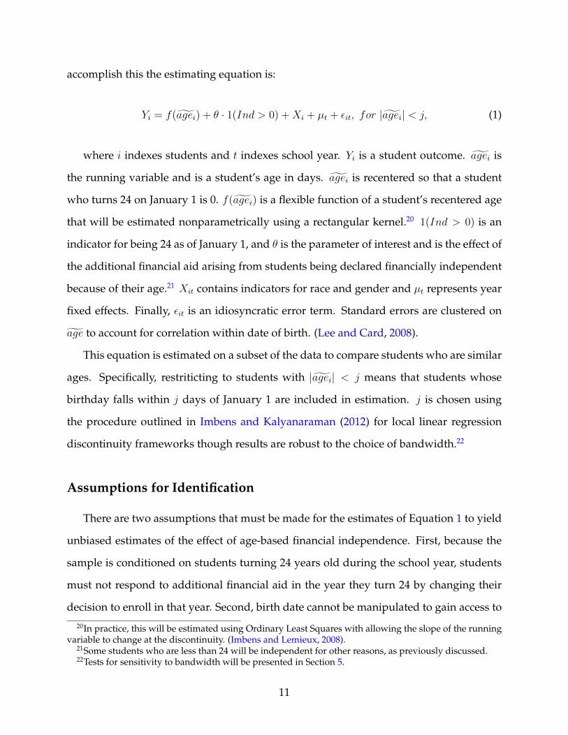
accomplish this the estimating equation is:
Yi = f(agei) + θ · 1(Ind > 0) +Xi + µt + εit, for |agei| < j, (1)
where i indexes students and t indexes school year. Yi is a student outcome. agei is
the running variable and is a student’s age in days. agei is recentered so that a student
who turns 24 on January 1 is 0. f(agei) is a flexible function of a student’s recentered age
that will be estimated nonparametrically using a rectangular kernel.20 1(Ind > 0) is an
indicator for being 24 as of January 1, and θ is the parameter of interest and is the effect of
the additional financial aid arising from students being declared financially independent
because of their age.21 Xit contains indicators for race and gender and µt represents year
fixed effects. Finally, εit is an idiosyncratic error term. Standard errors are clustered on
age to account for correlation within date of birth. (Lee and Card, 2008).
This equation is estimated on a subset of the data to compare students who are similar
ages. Specifically, restriticting to students with |agei| < j means that students whose
birthday falls within j days of January 1 are included in estimation. j is chosen using
the procedure outlined in Imbens and Kalyanaraman (2012) for local linear regression
discontinuity frameworks though results are robust to the choice of bandwidth.22
Assumptions for Identification
There are two assumptions that must be made for the estimates of Equation 1 to yield
unbiased estimates of the effect of age-based financial independence. First, because the
sample is conditioned on students turning 24 years old during the school year, students
must not respond to additional financial aid in the year they turn 24 by changing their
decision to enroll in that year. Second, birth date cannot be manipulated to gain access to
20In practice, this will be estimated using Ordinary Least Squares with allowing the slope of the runningvariable to change at the discontinuity. (Imbens and Lemieux, 2008).
21Some students who are less than 24 will be independent for other reasons, as previously discussed.22Tests for sensitivity to bandwidth will be presented in Section 5.
11

treatment. If either birth date manipulation or differential enrollment occurs, this would
appear as additional students who are 24 years or older as of January 1.
If students anticipate the additional financial aid available to independent students,
they may change their enrollment or reenrollment in response to additional financial aid.
If this occurs and enrollment is affected, then conditioning the sample on students who
turn 24 will yield biased estimates that conflate the effect of additional financial aid on
enrolled students and the change in sample composition arising from additional financial
aid.
Students do not appear to alter their enrollment decisions in the year they turn 24
based on financial independence. To check for this, in Figure 2 and Table 2 I exam-
ine the re-enrollment probabilities of 23-year-old students. Because I focus on seniors,
re-enrollment is how enrollment-induced changes in financial aid would manifest them-
selves. If financial independence altered enrollment decisions, it would appear as a dis-
crete change in the re-enrollment probabilities of 23–year–old students. The estimated
change in re-enrollment probability for students who will receive additional aid financial
is 0.0027 with a standard error of 0.0038. The robustness of this estimate to various band-
widths can be seen in Figure 6 where estimates and 95% confidence intervals are plotted
for bandwidths from 50 days to 150 days. The lack of an enrollment effect is seen in Fig-
ure 2. This can also be seen in Figure 1, Panel B, in which there is no discontinuity in the
density of students enrolling in the year they turn 24.
The lack of a response may be because the age rule governing independent status and
the consequence of financial independence are not widely known. It may also be that
older students who have typically accumulated substantial credits do not change their
reenrollment based on financial aid. Given that there is no measured effect on reenroll-
ment, I continue to condition the sample on enrollment in the year a student turns 24.
This lack of an (re)enrollment effect allows an examination of the effect of financial aid on
student outcomes apart from enrollment effects.
12

A second assumption for identification is that birth date is not manipulated to gain
access to the financial independence. Obviously, a student’s true birth date is not manip-
ulable by the student. Students do have incentives to misreport their birth date to gain
additional dollars, but the reported birth date is verified by comparison with Social Se-
curity Administration records. Students cannot manipulate their birth date, but parents
may manipulate their child’s birth date. There is evidence that birth dates are manip-
ulated around January 1 by parents in response to tax incentives (LaLumia et al., 2015;
Schulkind and Shapiro, 2014). This issue is discussed in Appendix Section A.2 and found
to likely affect only a very small number of students born within a few days of January 1.
To avoid any issues associated with potential retiming of births, the preferred speci-
fication will be a regression discontinuity “donut” estimator (Almond and Doyle, 2011),
in which the three days on either side of January 1 are omitted. The results are quanti-
tatively and qualitatively very similar if those three days are included; these results are
presented in Appendix Table A2. A formal McCrary test, after excluding 3 days around
January 1st, yields a point estimate of -.015 with a standard error of .013. 23
Section A.3 in the Appendix and Table A3 confirm that predetermined student char-
acteristics do not change discontinuously at the threshold.
Because of three qualifying conditions—1) there is no change in reenrollment proba-
bilities for 23-year-olds, 2) students are unable to manipulate their date of birth, and 3)
observed covariates do not vary discretely by eligibility status—the testable assumptions
of the regression discontinuity estimator are met and the results can be interpreted as the
causal impact of age-based financial independence on student outcomes.
23The inclusion of students just in the 3 day window yields an estimate of .054 with a standard error of.010. This discontinuity is clearly seen in Figure 1 but is notably absent when excluding 3 days aroundJanuary 1.
13

5 Results
Educational Outcomes
University students see substantial changes in financial aid arising from financial in-
dependence. This is documented in Figure 3 and Table 3. Students who are financially
independent appear on the right of the figures and receive an additional $966 in grant
dollars, the bulk of which comes in the form of increased Pell Grants ($806). They also
take out an additional $486 in loans. Between grants and loans, this represents a signifi-
cant change to student finances totaling over $1,452. One important caveat is that the data
do not contain private loans but do contain state loans such as the College Access Loan
(CAL Loan). Federal loans typically offer better interest rates than private loans and offer
access to a variety of repayment plans generally unavailable in the private market, in-
cluding income-based repayment, income-contingent repayment, graduated repayment,
or extended repayment. As a result, some of the increase in the amount of federal and
state loans could be students switching from private loans to federal and state loans. Fed-
eral loans are by far the most common type of loans, and private student loans make up
about 10 percent of student debt issued since 2009 (College Board , 2015). If financial inde-
pendence induced switching from private loans to federal and state loans, the estimated
increase in loan aid would overstate the degree to which students borrowed additional
money. Because the increase in federal loans ($864) is smaller than the increase in both
state and federal loans ($485) federal loans do appear to crowd out state loans, but not
completely.
This large change in financial aid allows an examination of whether student outcomes
are affected by financial aid. The effect on student outcomes are presented in Figure 4
and Table 3. Financial independence increases student credit hours attempted by 0.39. In
attempting more credits, students could see their GPA decrease if they do not change the
time devoted to studying. However, despite the larger class load, the student GPAs are
14

unaffected, with an estimated discontinuity of 0.001 and a 95 percent confidence interval
of –0.022 to 0.025. The additional financial aid increased student credits attempted but
did not reduce performance in those credits.
Because seniors are attempting more credits and GPA is unaffected, graduation has the
potential to be affected. This is seen in Figure 4 and in Table 3. Students are 1.8 percentage
points more likely to graduate in the year they turn 24 (in the tables this is designated
“Grad 4yr this year”) as a result of additional financial aid. This discontinuity is clearly
visible in the figure and is statistically different from zero at the 1 percent level. There
is an accompanying dip in the probability of enrolling in the next year, which provides
evidence that financial aid causes some students to graduate and not enroll in the next
year.
The increased graduation in the year of financial aid receipt could either be a result
of retiming graduation by encouraging students to graduate earlier than they otherwise
would have, or it could arise from students graduating who otherwise would not. To
investigate this graduation in either the year students turn 24 or the year afterward is
considered. The estimated coefficient (“Grad 4yr Next Year” in the table) is 0.002, which
suggests that additional financial aid retimed graduations rather than induced gradua-
tion among students who not otherwise have graduated.
While there is a positive effect on graduation in the year the money is received, it is
relatively small. The 1.8 percentage point increase represents a 4 percent increase in the
graduation rate during the school year a student turns 24. The increase comes at a cost of
$966 in grants. Assuming that all of the graduation effects are driven by grants, it costs
$55,234 in grants for one student to graduate one year earlier. The cost would be even
higher after accounting for additional subsidies received for loans. College enrollees in
the sample earn $12,219, and students who graduate in the year they turn 24 earn $26,923
in the year they turn 25. This means that graduating a year earlier corresponds to roughly
a $14,704 difference in earnings. However, for the sample taken as a whole the benefits of
15

an additional year in the labor market do not exceed the costs associated with one student
graduating a year earlier. I will explore whether additional financial aid is cost effective
by exploring students with different levels of income in Section 5.
Mechanisms
I now investigate mechanisms for the increased credits attempted and reduced time
to degree, including reduced time spent working during college and binding credit con-
straints.
Labor Supply during College
Despite the large number of students in the labor force and the large amount of federal
financial aid available, very few studies have attempted to identify the effects of financial
aid on student earnings. Broton et al. (2016) use random assignment of a state need-
based grant to examine student responses to survey questions about work. They find
that students receiving financial aid reduced hours worked by about 14 percent. Scott-
Clayton (2011) examines the effect of a merit scholarship in West Virginia that affected
enrollment and finds that scholarships reduce earnings in some specifications but not in
others.24
Additional financial aid may allow students to reduce time spent working. Using
Unemployment Insurance earnings data, in Figure 5 I explore whether students who are
24The sensitivity Scott-Clayton (2011) to specificaiton may be because the identification strategies mea-sure different local average treatment effects or because there is a bias in one or both of the estimates arisingfrom those strategies. Also, Scott-Clayton and Park (2015) use a regression discontinuity to examine the ef-fect of replacing federal loans with the Pell grants for community college students and find that grantsreduce earnings and increase full-time enrollment. However, there is a discontinuity in the density of therunning variable, which suggests the results may be biased.
In related work, many studies have tried to quantify the effect of working on educational outcomes. Thegeneral finding has been that working in college decreases GPA (Kalenkoski and Pabilonia, 2010; Stine-brickner and Stinebrickner, 2003) and credits accumulated (Darolia, 2014; Triventi, 2014). These studiesmotivate studying the effect of financial aid on labor supply. The financial aid-induced reductions in earn-ings and accelerated graduation results in this paper are consistent with the aforementioned prior studieson the effects of employment on student outcomes.
16

declared financially independent based on age change their earnings in response to the
additional grants and loans they receive. Financially independent university students
do not adjust the probability of positive earnings. The coefficient on whether students
have positive earnings is –0.5 percentage points with a standard error of 0.5 percentage
points. This rules out reasonably small reductions in the probability of earnings up to –1.5
percentage points. Despite no change in the probability of working, there is significant
change in earnings during college seen in Figure 5, Panel B. Students who are financially
independent by age 24 see their earnings decrease by $511. This represents about 35 per-
cent of the increase in grants and loans, or 55 percent of the increase in grants. Financial
aid appears to crowd out earning by reducing labor supply on the intensive margin but
does not seem to affect extensive margin labor supply.
Interpreting the change in earnings requires some caution. In Table A4, I perform a
placebo exercise where I use the same specifications except I examine students turning 21,
22, or 23 during the school year. For the 22 and 23 year old subset, there are discontinuities
of $162 and $220 respectively that are significant at the 5% level. These two placebo
exercises are the only two that are significant at the 5% level and 21-year-old students do
not see reduced earnings at the threshold. Because this occurs for both 22 and 23-year-old
students this is likely to not be the result of gaming eligibility to insure additional grant
aid. This could be the result of chance as there are 18 placebo outcomes considered and 2
significant discontinuities at the 5% level. Moreover, the effects on earnings are somewhat
sensitive to the choice of bandwidth as can be seen in Figure 6, with smaller bandwidths
yielding smaller, insignificant effects on earnings. Given the sensitivity to bandwidth and
the issues in the placebo test, I interpret the evidence on earnings as being suggestive but
not definitive of earnings declines due to additional aid.25
25Interpreting the estimates of the effect of additional financial aid on earnings requires additional cau-tion, because earnings for students employed by the university they attend are not included in UI earn-ings records unless the student is employed as part of the federal work-study program. There is furtherdiscussion of on-campus employment in Appendix Section A.4, but if anything, the lack of on-campus,non-work-study earnings likely results in an underestimate of the effect of financial aid on earnings.
17

Unfortunately, in this setting, it is impossible to completely disentangle the effect of
additional eligibility for student loans from the effect of additional grant money on earn-
ings. In the section on heterogeneous effects by family income, I will examine groups of
students who saw small (or no) increases in grants and larger increases in loans to see if
there are differences by the type of aid received. Given the earlier results on completion,
the suggestive findings on earnings support the idea that working during college slows
down time to degree.
Credit Constraints
Financial aid may reduce time to degree because it eases binding credit constraints.
This paper estimates to what degree increased financial aid eases these constraints. Many
studies have attempted to identify whether binding credit constraints affect college en-
rollment and graduation. Early studies tended to find that credit constraints were not
prevalent (Cameron and Heckman, 1998; Cameron and Taber, 2004; Carneiro and Heck-
man, 2002; Keane and Wolpin, 2001). However, recent studies have shown borrowing
constraints matter for educational investment (Belley and Lochner, 2007; Brown et al.,
2012; Cowan, 2016; Lovenheim, 2011; Stinebrickner and Stinebrickner, 2008).
Independent students have access to higher yearly and aggregate federal student loan
limits than do dependent students. This provides an opportunity to test for credit con-
straints among enrolled college students. Specifically, how does financial independence
affect the number of students borrowing above the amount that would be allowed had
they been born a few days later? Any student, regardless of assessed financial need, may
borrow the maximum amount of federal unsubsidized loans as long as the amount of
loans does not exceed unmet financial need.
Figure 3 and Table 3 investigate this question. Panel C shows that there is a 15% in-
crease in the number of students borrowing more federal loans than the dependent max-
imum. This suggests that 15% of students face binding credit constraints and financial
18

independence eases their credit constraints by raising their borrowing limit. This esimate
is similar in magnitude to Stinebrickner and Stinebrickner (2008).
There are three important caveats for the estimation of the number of students who
are credit constrained– private loans, changes in grant aid, and behavioral factors. As
previously discussed, federal loans are the bulk of the market for student loans and are
more attractive. As a result, students are likely to exhaust their federal loan eligibility
before turning to the private loan market. In the 2012 National Postsecondary Student
Aid Study (NPSAS), 9.6 percent of students who reported taking out less than the statu-
tory maximum of federal student loans reported having taken out private loans, which
suggests that nearly all students will exhaust federal student loan eligibility before taking
out private loans.
Financial independence not only changes the maximum amount of loans students
have access to but increases grants and eligibility for subsidized loans. To partially ad-
dress this issue, I will examine students who had received a Pell Grant or a zero EFC in the
previous year in the section on heterogeneity. These students see smaller (or no) changes
in grants and subsidized loans, and as a result, looking at them can be more informative
of what might happen if subsidized loans and grants were unchanged. The results are
not substantively different for this group of students.
Loan take up has been shown to depend on the amount of loan offer. In the present
setting, the default loan offer increases for students who are independent. Marx and
Turner (2016) use a randomized controlled trial and demonstrate that the default of pack-
aging loan amounts at their maximum affects loan take up. They also show that offering
students their maximum loan they are eligible for affects the number of students taking
the maximum loan for which they are eligible. The results from Marx and Turner (2016)
suggest that the measure of credit constraints in this paper may be imperfect due to be-
havioral responses to loan offers.
19

Heterogeneity
I examine heterogeneity by a measure of parental income, which affects the size of the
change in financial aid. In Table 4, separate discontinuities are estimated for three groups
of students: 1) students who had a zero EFC when they were 23 years old, 2) students
who received a Pell grant when they were 23 years old, and 3) students who did not
receive a Pell Grant when they were 23 years old. These groups are examined separately
because changes in financial aid arising from age-induced financial independence are
quite different based on family income.
Students who previously received a zero EFC are examined in Column 1 of Table 4
and see no change in grants or subsidized loans. These are the neediest students in the
sample, and so the exclusion of parental income and assets does not affect their eligibil-
ity for grants or subsidized loans. However, these students do increase borrowing by
$723. Despite only seeing an increase in student loans, age-induced financial indepen-
dence causes 4 percent of students to speed up graduation by one year. Students who
previously received a zero EFC appear to reduce earnings by roughly the same amount
as the sample as a whole at $495, but this is imprecisely estimated. The reduction in earn-
ings is approximately 65 percent of the increase in loans. The larger effects on educational
outcomes is somewhat surprising given the lack of a change in grants. However, the in-
creased loans are likely to help these students most, as they are the neediest in the sample.
These estimates demonstrate the academic benefits of increased access to student loans
for the poorest students.
Students who previously received a zero EFC can be helpful in understanding how
many students are credit constrained because they experience no change in grants or sub-
sidized loans as a result of age-induced financial independence. Among these students,
age-induced financial independence increases borrowing above the dependent maximum
by 16.2 percentage points which is larger than the sample as a whole
20

The second column examines students who received a Pell Grant when they were 23.26
These students see a $374 increase in grants, a $727 increase in total loans for age-induced
changes in financial independence. They are slightly more likely to graduate than the full
sample as a result of financial aid, with 2.85 percent graduating one year earlier. They
also reduce earnings and appear to be credit constrained at slightly higher rates to the
sample as a whole.
The third column of Table 4 examines students who did not receive a Pell Grant when
they were 23 years old. These students are wealthier, so excluding parental income in-
duces larger changes in need-based financial aid. They see a $1232 increase in grants and
a $370 increase in loans. Despite a much larger change in financial aid, the effect on time
to degree is smaller, with 1.3 percent reducing time to degree by one year though this is
not significant at the 5% level. They reduce earnings by $520 and have a smaller number
of credit constrained students at 13.7 percentage points.
The estimate for the fraction of students constrained does not vary substantially across
student income. However, students who previously did not receive the Pell have a smaller
estimate for the number of constrained students than students who previously had re-
ceived a Pell Grant (13.7 versus 17.4 percentage points).
The heterogeneity analysis shows that the cost of reducing time to degree by one year
varies substantially by family income. For students who had previously received an EFC
of zero, there is no direct cost from grants. The increase in loans for independent students
reduces time to graduation. Essentially, this decreased time to degree (and increased time
in the labor market) comes at cost of administering student loans. For students who had
previously received a Pell Grant, an additional $13,108 in grants decreases time to degree
by one year.27 This is very similar to how much more graduates in the sample make as
compared to students enrolled in college. For students who had previously received a
Pell Grant, additional grant aid is likely to be efficient, as its cost is roughly equal to the
26Students with a zero EFC in the year they turned 23 are a subset of this sample.27This abstracts from the costs of subsidized loans or program administration costs.
21

gain in earnings that a student sees from an additional year in the labor market. For
students who had not previously received a Pell Grant, reducing time to degree costs
$98,536 which is substantially more costly than the benefit of an additional year in the
labor market.
Taken together, the results on heterogeneity by previous Pell receipt suggest a few
things: Financial independence gives more resources to relatively wealthier students. De-
spite this, the reduced time to graduation seems to be larger for needier students. In fact,
aid to students who qualified for the Pell Grant in the year they turned 23 is likely to be
efficient, as the benefits to the students are less than or equal to the costs. These results
on heterogeneity highlight the educational attainment benefits of targeting financial aid
to the neediest students.
5.1 Other Classifications
The focus of this paper is on seniors turning during an academic year. However, the
same change in dependent status occurs for students who are not seniors. These students
are considered in Table 5. There are very few students turning 24 as freshman and the
results presented are imprecise as a result. However, the point estimates for freshman are
positive for hours attempted and reenrollment.
However, sophomores and juniors have more students and there is some increased
precision. In both cases, students are more likely to persist to the next year. Sophomores
are 7.9 percentage points more likely and juniors are 2.6 percentage points more likely. Ju-
niors also attempt .51 more credit hours. Student earnings are not affected for Freshman,
Sophomores, and Juniors.
These students provide further evidence that additional financial aid provide benefits
to students before their senior year. Although 24 year old students are a particular sam-
ple this shows that financial aid affects older students who are not as far along in their
schooling.
22

Robustness
Two additional robustness checks are performed to make sure the results are not spu-
rious. The first is to check the choice of bandwidth and is presented in Figure 6. This
figure considers a main result of the paper, which finds that students who are financially
independent and receive additional financial aid are more likely to graduate in the year
they receive the aid and reduce their earnings. Each of the dots represents an estimated
discontinuity, along with 95 percent confidence intervals for different bandwidth choices.
For graduation in the year students turn 24, the estimate is stable across bandwidths and
is statistically different from zero starting with the bandwidth of 80 days.
For earnings, smaller bandwidths tend to deliver smaller estimates, but once the band-
width includes 90 days it is statistically different from zero. This figure shows that the
effect on earnings is somewhat sensitive to the choice of bandwidth
I also use students turning 21, 22, and 23 as placebo exercises to see if student out-
comes systematically vary at January 1. These results are presented in Table A4 and are
discussed in Appendix Section A.5. If students anticipated the change in financial aid, we
would likely see changes in student outcomes for these students. However, student out-
comes do not significantly differ at this same threshold for other ages with the exception
of earnings as previously discussed.
6 Discussion and Conclusion
This paper links three trends in higher education: 1) higher tuition, 2) increasing time
to degree, and 3) increased earnings in college. In particular, the price of college causally
increases time to degree and I present suggestive evidence that it increases student labor
supply. The effects of college price on inframarginal students are important because they
affect many students and are implicitly included in every financial aid and tuition policy
considered but are rarely measured.
23

Several policy lessons emerge from this paper. First, proposals to change tuition or
financial aid should consider the implications of their decisions on time to degree. In fact,
this may be the bulk of the effect, as changes in price are likely to induce relatively small
changes in enrollment while affecting all enrolled students.
Second, the change in financial aid associated with financial independence is poorly
targeted. The largest increases in aid go to students who come from the most affluent
backgrounds. As a result, the benefits from the change in independence (namely one
additional year in the labor market) do not outweigh the costs for the sample as a whole.
However, for poorer students who see smaller changes in aid, the effects on time to degree
are comparatively larger. For students who had previously had a zero EFC, time to degree
is reduced simply by allowing additional borrowing of unsubsidized loans.
The heterogeneous effects of financial aid by family income underscore how targeting
financial aid to needier students improves student outcomes relative to aid for wealthier
students. This is particularly important for evaluating policy that reduces the price of
college for all students.
24

References
Almond, D. and Doyle, J. J. (2011). After midnight: A regression discontinuity design in
length of postpartum hospital stays. American Economic Journal. Economic Policy, 3(3):1–
34.
Anderson, D. M. and Goldrick-Rab, S. (2016). Aid after enrollment: Impacts of a statewide
grant program at public two-year colleges.
Angrist, J., Autor, D., Hudson, S., and Pallais, A. (2014). Leveling up: Early results from
a randomized evaluation of post-secondary aid. Working Paper No. 20800, National
Bureau of Economic Research, Cambridge, MA.
Barr, A. (2015). From the battlefield to the schoolyard. Journal of Human Resources, 50(3).
Barr, A. (2016). Fighting for education: Veterans and financial aid. Working paper, Uni-
versity of Virginia.
Belley, P. and Lochner, L. (2007). The changing role of family income and ability in deter-
mining educational achievement. Journal of Human Capital, 1(1):37–89.
Bettinger, E. (2015). Need-based aid and college persistence the effects of the ohio college
opportunity grant. Educational Evaluation and Policy Analysis, 37(1 suppl.):102S–119S.
Bettinger, E., Gurantz, O., Kawano, L., and Sacerdote, B. (2016). The long run impacts
of merit aid: Evidence from californias cal grant. Technical report, National Bureau of
Economic Research, Cambridge, MA.
Bound, J., Lovenheim, M. F., and Turner, S. (2010). Why have college completion rates de-
clined? an analysis of changing student preparation and collegiate resources. American
Economic Journal: Applied Economics, 2(3):129–157.
Bound, J., Lovenheim, M. F., and Turner, S. (2012). Increasing time to baccalaureate degree
in the united states. Education Finance and Policy, 7(4):375–424.
25

Broton, K. M., Goldrick-Rab, S., and Benson, J. (2016). Working for college: The causal
impacts of financial grants on undergraduate employment. Educational Evaluation and
Policy Analysis, 38(3):477–494.
Brown, M., Scholz, J. K., and Seshadri, A. (2012). A new test of borrowing constraints for
education. Review of Economic Studies, 79(2):511–538.
Cameron, S. V. and Heckman, J. J. (1998). Life cycle schooling and dynamic selection bias:
Models and evidence for five cohorts of american males. Journal of Political Economy,
106(2):262–333.
Cameron, S. V. and Taber, C. (2004). Estimation of educational borrowing constraints
using returns to schooling. Journal of Political Economy, 112(1):132–182.
Carneiro, P. and Heckman, J. J. (2002). The evidence on credit constraints in post-
secondary schooling. Economic Journal, 112(482):705–734.
Carnevale, A. P., Smith, N., Melton, M., and Price, E. W. (2015). Learning while earning:
The new normal. Technical report.
Castleman, B. L. and Long, B. T. (2016). Looking beyond enrollment: The causal effect
of need-based grants on college access, persistence, and graduation. Journal of Labor
Economics, 34(4):1023–1073.
Cohodes, S. and Goodman, J. (2014). Merit aid, college quality, and college completion:
Massachusetts adams scholarship as an in-kind subsidy. American Economic Journal:
Applied Economics, 6(4):251–285.
College Board (2015). Trends in student aid 2015. College Board, Trends in Higher
Education, New York.
Cowan, B. W. (2016). Testing for educational credit constraints using heterogeneity in
individual time preferences. Journal of Labor Economics, 34(2):363–402.
26

Darolia, R. (2014). Working (and studying) day and night: Heterogeneous effects of work-
ing on the academic performance of full-time and part-time students. Economics of Ed-
ucation Review, 38:38–50.
Dillender, M. (2014). Do more health insurance options lead to higher wages? evidence
from states extending dependent coverage. Journal of Health Economics, 36(1):84–97.
Dynarski, S. (2008). Building the stock of college-educated labor. Journal of Human Re-
sources, 43(3):576–610.
Dynarski, S. and Scott-Clayton, J. (2015). Tax benefits for education: History and
prospects for reform. Technical report.
Garibaldi, P., Giavazzi, F., Ichino, A., and Rettore, E. (2012). College cost and time to com-
plete a degree: Evidence from tuition discontinuities. Review of Economics and Statistics,
94(3):699–711.
Goldrick-Rab, S., Kelchen, R., Harris, D., and Benson, J. (2016). Reducing income inequal-
ity in educational attainment:experimental evidence on the impact of financial aid on
college completion. American Journal of Sociology, 121(6):1762–1817.
Hoekstra, M. (2009). The effect of attending the flagship state university on earnings: A
discontinuity-based approach. Review of Economics and Statistics, 91(4):717–724.
Imbens, G. and Kalyanaraman, K. (2012). Optimal bandwidth choice for the regression
discontinuity estimator. Review of Economic Studies, 79(3):933–959.
Imbens, G. W. and Lemieux, T. (2008). Regression discontinuity designs: A guide to
practice. Journal of Econometrics, 142(2):615–635.
Kalenkoski, C. M. and Pabilonia, S. W. (2010). Parental transfers, student achievement,
and the labor supply of college students. Journal of Population Economics, 23(2):469–496.
27

Keane, M. P. and Wolpin, K. I. (2001). The effect of parental transfers and borrowing
constraints on educational attainment. International Economic Review, 42(4):1051–1103.
LaLumia, S., Sallee, J. M., and Turner, N. (2015). New evidence on taxes and the timing of
birth. American Economic Journal: Economic Policy, 7(2):258–293.
Lee, D. S. and Card, D. (2008). Regression discontinuity inference with specification error.
Journal of Econometrics, 142(2):655–674.
Lovenheim, M. F. (2011). The effect of liquid housing wealth on college enrollment. Journal
of Labor Economics, 29(4):741–771.
Marx, B. M. and Turner, L. J. (2016). Student loan nudges: Experimental evidence on
borrowing and educational attainment. Working Paper.
Murphy, R. and Wyness, G. (2016). Paying for success: The causal effect of financial
assistance on university achievement and completion. Working Paper.
National Center for Education Statistics (2013). Digest of education statistics: 2012.
National Center for Education Statsitics (2012). National postsecondary student aid study
2011-12.
Oreopoulos, P. and Petronijevic, U. (2013). Making college worth it: A review of research
on the returns to higher education. Technical report, National Bureau of Economic
Research.
Oreopoulos, P. and Salvanes, K. G. (2011). Priceless: The nonpecuniary benefits of school-
ing. Journal of Economic Perspectives, 25(1):159–184.
Ost, B., Pan, W., and Webber, D. (2016). The returns to college persistence for marginal
students: Regression discontinuity evidence from university dismissal policies. Tech-
nical Report No. 9799, IZA Discussion Paper, Bonn, Germany.
28

Schulkind, L. and Shapiro, T. M. (2014). What a difference a day makes: Quantifying
the effects of birth timing manipulation on infant health. Journal of Health Economics,
33(C):139–158.
Scott-Clayton, J. (2011). On money and motivation: A quasi-experimental analysis of
financial incentives for college achievement. Journal of Human Resources, 46(3):614–646.
Scott-Clayton, J. (2012). What explains trends in labor supply among u.s. undergraduates?
National Tax Journal, 65(1):181–210.
Scott-Clayton, J. and Minaya, V. (2014). Should student employment be subsidized? con-
ditional counterfactuals and the outcomes of work-study participation. Working Paper
no. 20329, National Bureau of Economic Research.
Scott-Clayton, J. and Park, R. S. (2015). The impact of pell grant eligibility on community
college students financial aid packages, labor supply, and academic outcomes. Paper
Presented at the Association for Education Finanace and Policy Fortieth Annual Con-
ference.
Scott-Clayton, J. and Zafar, B. (2016). Financial aid, debt management, and socioeconomic
outcomes: post-college effects of merit-based aid. Technical report, National Bureau of
Economic Research.
Seftor, N. S. and Turner, S. E. (2002). Back to school: Federal student aid policy and adult
college enrollment. Journal of Human Resources, 37(2):336–352.
Sjoquist, D. L. and Winters, J. V. (2012). Building the stock of college-educated labor
revisited. Journal of Human Resources, 47(1):270–285.
Stinebrickner, R. and Stinebrickner, T. (2003). Working during school and academic per-
formance. Journal of Labor Economics, 21(2):473–491.
29

Stinebrickner, R. and Stinebrickner, T. (2008). The effect of credit constraints on the college
drop-out decision: A direct approach using a new panel study. The American Economic
Review, 98(5):2163–2184.
Triventi, M. (2014). Does working during higher education affect students academic pro-
gression? Economics of education review, 41(C):1–13.
U.S. Department of Education (2013a). 2011-12 national postsecondary student aid study.
Technical report, National Center for Education Statistics, Washington, DC.
U.S. Department of Education (2013b). Student financial assistance fiscal year 2013 budget
request. Technical report, Washington, D.C.
Zimmerman, S. (2014). The returns to four-year college for academically marginal stu-
dents. Journal of Labor Economics, 32(4):711–754.
30

7 Figures and Tables
Figure 1: Density of Birth Dates
(a) 4yr (b) 4yr Donut
NOTE: Panel A plots the number of students born on each day of the year, and PanelB replicates that plot but removes students born within three days of January 1. Thehorizontal axis is recentered age in days such that 0 is 24 years old on January 1. andThe data come from administrative records of the THECB and include the 2002–2003 to2013–2014 school years.
Figure 2: Reenrollment of 23-year-olds
NOTE: This figure plots the fraction of 23-year-olds who re-enroll in the year they turn 24by their recentered birth date. The horizontal axis is recentered age in days such that 0 is24 years old on January 1. The data come from administrative records of the THECB andinclude the 2002–2003 to 2013–2014 school years.
31

Figure 3: Four-Year Colleges, Financial Aid
(a) Grants (b) Loans
(c) Borrow More than Unsub. Max
NOTE: Panel A plots the average amount of grants received by students by their age asof January 1. Panel B plots the amount of loans taken out by the students by their ageas of January 1 and Panel C plots the fraction of students who borrow above the annualfederal maximum for dependent students. The horizontal axis is recentered age in dayssuch that 0 is 24 years old on January 1. Each dot represents the average for a group of10 birth dates. The size of the dot is proportional to the number of students for whichthe average is computed. The data are from administrative records of the THECB andinclude the 2002–2003 to 2013–2014 school years.
32

Figure 4: Four-Year Colleges, Educational Outcomes
(a) Hours Attempted (b) Grad this Year
(c) Re Enroll Next Year (d) Grad Next Year
NOTE: Panel A plots the number of credit hours attempted by student age as of January1. Panel B plots the probability of graduating in the year a student turns 24 by birth date.Panel C plots the probability of reenrolling in the year after a student turns 24 by birthdate. Panel D plots the probability of graduating by the year after a student turns 24 bybirth date. The horizontal axis is recentered age in days such that 0 is 24 years old onJanuary 1. Each dot represents the average for a group of 10 birth dates. The size of thedot is proportional to the number of students for which the average is computed. Thedata are from administrative records of the THECB and include the 2002–2004 to 2013–2014 school years.
33

Figure 5: Four-Year Colleges, Earnings Outcomes
(a) Employment (b) Earnings
NOTE: Panel A plots the fraction of students with nonzero earnings in the year they turn24 by their age as of January 1. Panel B plots earnings by birth date. The size of thedot is proportional to the number of students for which the average is computed. Thehorizontal axis is recentered age in days such that 0 is 24 years old on January 1. The datacome from administrative records of the TWC and include the 2002–2003 to 2013–2014school years.
34
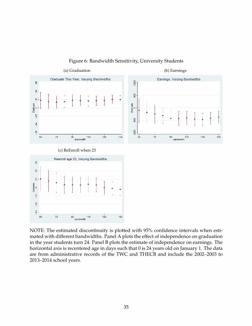
Figure 6: Bandwidth Sensitivity, University Students
(a) Graduation (b) Earnings
(c) ReEnroll when 23
NOTE: The estimated discontinuity is plotted with 95% confidence intervals when esti-mated with different bandwidths. Panel A plots the effect of independence on graduationin the year students turn 24. Panel B plots the estimate of independence on earnings. Thehorizontal axis is recentered age in days such that 0 is 24 years old on January 1. The dataare from administrative records of the TWC and THECB and include the 2002–2003 to2013–2014 school years.
35

Table 1: Summary Stats
Variable Obs Mean Std. Dev.Male 227,848 0.49 0.50White 227,848 0.49 0.50Black 227,848 0.10 0.30Hispanic 227,848 0.30 0.46Asian 227,848 0.05 0.21Hours attempted 227,848 22.09 10.36Enroll next year 227,848 0.46 0.50Graduate current year 227,848 0.44 0.50Graduate next year 227,848 0.70 0.46GPA 227,848 2.70 0.97Borrow at unsub Max 227,848 0.06 0.24Borrow at sub max 227,848 0.12 0.32Borrow more than unsub max 227,848 0.17 0.38Total grants 227,848 2,168.59 3,125.50Pell 227,848 1,449.67 2,111.72Total loans 227,848 4,155.84 5,421.51Received Pell last year 227,848 0.30 0.46Earnings 227,848 12061.83 12424.1Positive earnings 227,848 0.79 0.41
NOTE: Summary statistics for the sample of seniors at Texas public universities from2002-2003 to 2013-2014 who are within 200 days of turning 24 during the school year. Thedata are from administrative records of the THECB and TWC and include the 2003–2004to 2013–2014 school years. Variables that refere to the current year refer to the academicyear in which students turn 24. Variables that refer to ”next year” refer to the academicyear in which students turn 24. Earnings correspond to earnings for the academic year(Q4 in year t-1 and Q1,Q2, and Q3 in year t.
36

Table 2: Reenrollment Probability of 23-Year-Old Students
Re-Enroll 4yr
Discontinuity 0.0027(0.0038)
Mean | Ineligible 0.5
Observations 257,723NOTE: This table estimates the change in the probability of reenrolling in the next schoolyear for students who turn 23 during the current school year. Students born December 29through January 3, are excluded as discussed in the text. The discontinuity is estimatedusing a window of birth dates of 100 days from January 1. Mean | Ineligible is the esti-mated value of the dependent variable at the discontinuity for ineligible students. Theregressions also include controls for gender and race. Standard errors are clustered onrecentered birth date and are in parentheses, with * p<0.1 ** p<0.05 *** p<0.01.
37
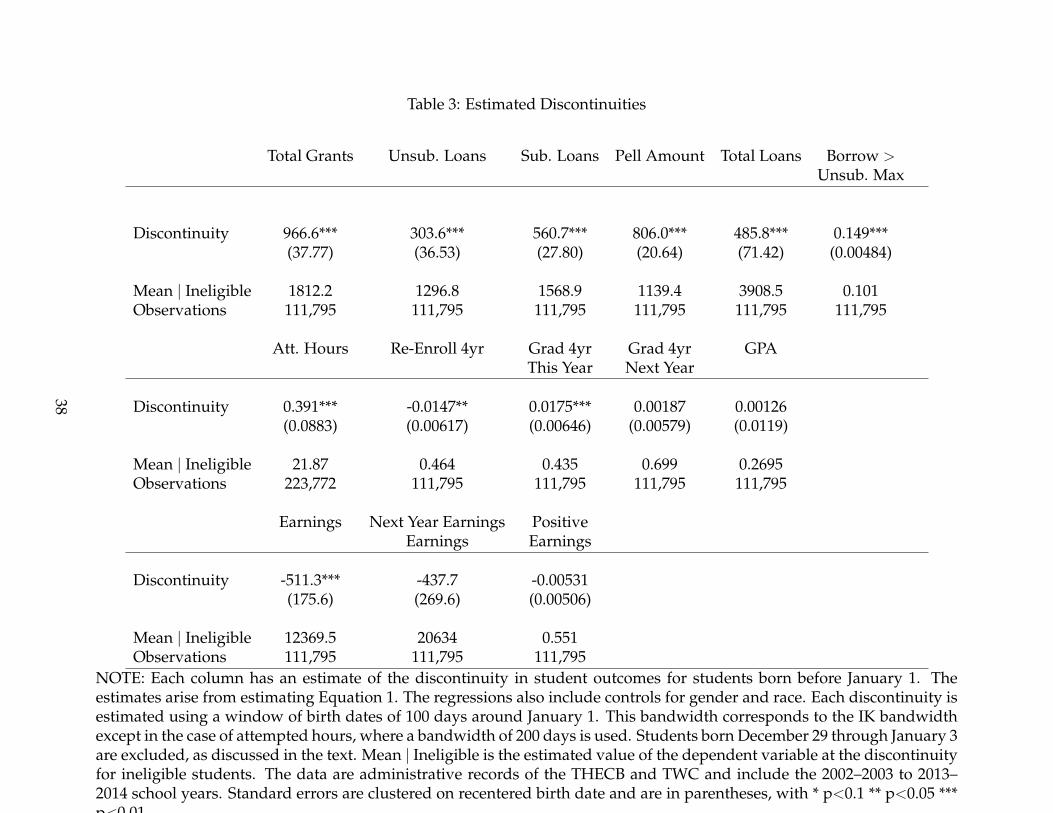
Table 3: Estimated Discontinuities
Total Grants Unsub. Loans Sub. Loans Pell Amount Total Loans Borrow >Unsub. Max
Discontinuity 966.6*** 303.6*** 560.7*** 806.0*** 485.8*** 0.149***(37.77) (36.53) (27.80) (20.64) (71.42) (0.00484)
Mean | Ineligible 1812.2 1296.8 1568.9 1139.4 3908.5 0.101Observations 111,795 111,795 111,795 111,795 111,795 111,795
Att. Hours Re-Enroll 4yr Grad 4yr Grad 4yr GPAThis Year Next Year
Discontinuity 0.391*** -0.0147** 0.0175*** 0.00187 0.00126(0.0883) (0.00617) (0.00646) (0.00579) (0.0119)
Mean | Ineligible 21.87 0.464 0.435 0.699 0.2695Observations 223,772 111,795 111,795 111,795 111,795
Earnings Next Year Earnings PositiveEarnings Earnings
Discontinuity -511.3*** -437.7 -0.00531(175.6) (269.6) (0.00506)
Mean | Ineligible 12369.5 20634 0.551Observations 111,795 111,795 111,795
NOTE: Each column has an estimate of the discontinuity in student outcomes for students born before January 1. Theestimates arise from estimating Equation 1. The regressions also include controls for gender and race. Each discontinuity isestimated using a window of birth dates of 100 days around January 1. This bandwidth corresponds to the IK bandwidthexcept in the case of attempted hours, where a bandwidth of 200 days is used. Students born December 29 through January 3are excluded, as discussed in the text. Mean | Ineligible is the estimated value of the dependent variable at the discontinuityfor ineligible students. The data are administrative records of the THECB and TWC and include the 2002–2003 to 2013–2014 school years. Standard errors are clustered on recentered birth date and are in parentheses, with * p<0.1 ** p<0.05 ***p<0.01.
38

Table 4: Heterogeneity Analysis
Previous 0 EFC Previous pell Previous No PellTotal Grants -129.0 373.6*** 1231.7***
(101.5) (71.31) (33.45)
Mean | Ineligible 4975.2 4411.2 659.1
Total Loans 723.3*** 727.7*** 370.9***(155.1) (121.2) (83.73)
Mean | Ineligible 5256.6 5486.7 3208.4
Grad 4yr in 0y 0.0396*** 0.0285*** 0.0125(0.0137) (0.0108) (0.00762)
Mean | Ineligible 0.406 0.433 0.437
Grad 4yr in 1y 0.0135 0.00871 -0.00122(0.0145) (0.0105) (0.00644)
Mean | Ineligible 0.694 0.712 -0.00122
Earnings -495.0 -507.1* -520.1**(352.9) (261.1) (204.2)
Mean | Ineligible 11368.9 11539 12737.6
Borrow >Unsub. Max 0.162*** 0.174*** 0.137***(0.0129) (0.00997) (0.00481)
Mean | Ineligible 0.19 0.184 0.0643
Observations 18,995 33,844 77,951NOTE: Each entry is an estimate of the discontinuity in student outcomes for studentsborn before January 1. The estimates arise from estimating Equation 1. The rows rep-resent different outcomes and the columns represent different estimating samples basedon student characteristics in the year they turn 23. The regressions also include controlsfor gender and race. Each discontinuity is estimated using a window of birth dates of100 days from January 1. Students born December 29 through January 3 are excluded asdiscussed in the text. Mean | Ineligible is the estimated value of the dependent variableat the discontinuity for ineligible students. The data are administrative records of theTHECB and TWC and include the 2002–2003 to 2013–2014 school years. Standard errorsare clustered on recentered birth date and are in parentheses, with * p<0.1 ** p<0.05 ***p<0.01.
39

Table 5: Other Classifications
Freshman Grants Loans Hours Enroll Next Year EarnDiscontinuity 157.3 303.9 0.280 0.0132 356.2
(145.5) (192.0) (0.349) (0.0306) (757.0)
Mean | Ineligible 1134.1 1741.2 13.94 0.439 10657Observations 4,687 4,687 9,354 4,687 4,687
Sophomore Grants Loans Hours Enroll Next Year EarnDiscontinuity 364.6*** 721.1*** 0.186 0.0794*** 104.4
(103.3) (161.2) (0.242) (0.0191) (491.1)
Mean | Ineligible 1577.3 2664.6 16.22 0.58 11953Observations 11,216 11,216 22,759 11,216 11,216
Junior Grants Loans Hours Enroll Next Year EarnDiscontinuity 510.9*** 609.7*** 0.510*** 0.0264** -116.8
(68.95) (121.8) (0.164) (0.0108) (309.1)
Mean | Ineligible 1688.2 3551 18.94 0.739 12265.3Observations 28,590 28,590 57,809 28,590 28,590
40

A Appendix
A.1 Changes resulting from Tax Aid
There are several reasons that the effects found in this paper are likely driven by fi-
nancial aid rather than tax aid. The first is that tax aid is disbursed for the prior financial
tax year no earlier than February. This date falls after students have made extensive and
intensive margin enrollment decisions for both semesters, which likely limits the extent
to which tax aid can influence student outcomes. Furthermore, a student’s tax liability is
likely to decrease as a result of the change, whereas family tax liability is likely to decrease
making the effect on student finances ambiguous. Last, federal tax aid more than doubled
in 2009. As a robustness check, I show that the results are not substantively different in
the years before or after this increase in tax aid in Table A1. For these reasons, the results
of this study will largely be interpreted as the effects of financial aid rather than of tax
aid.
Dependent status for tax purposes changes for a minority of students. In particular,
students must live at home for at least six months and provide less than half of their own
support. An upper bound on the number of students experiencing a change in depen-
dency status for tax purposes can be gleaned from the 2007–2008 National Postsecondary
Student Aid Study. The NPSAS contains information students’ residence with parents
while they are enrolled. Students at four-year schools in Texas who are from 23.5 to 24.5
years old on January 1 live with their parents 15.0 percent of the time (U.S. Department
of Education, 2013a). This number is an upper bound on the number of students affected
by the change in tax status, because some of those who live at home may receive less than
half of their support from their parents.
If a student is declared independent, all else being equal, the parent’s tax liability will
increase, as they no longer can claim a dependent exemption or any of the education
tax credits. If parents were eligible for the Earned Income Tax Credit (EITC), they are
41

likely to see EITC benefits decrease, as the number of eligible children will be reduced.
The students will have their personal tax liability decrease, as they will be able to use
the education tax credits on their tax return instead of their parents’ using the education
tax credits. In general, the family’s total tax liability will weakly increase as credits or
deductions are shifted from parents with relatively high marginal tax rates to students
with relatively low marginal tax rates.28
Financial independence is associated with (weakly) reduced family tax aid but in-
creased student tax aid. How this affects total resources toward college depends on
how parents and older students split changes in wealth from marginal tax changes. I
am not aware of any studies that examine how families split such tax changes, and data
on within-family transfers would be required to answer the question. Tax aid is never
“disbursed” per se, and households may differ in the timing of realizing tax benefits.
One test for the impact of tax credits for college is to consider the time before the
large expansion of tax credits that occurred in 2009. Tax expenditures increased by 140
percent in 2009. Results from 2002–2003 to 2007–2008 are presented in Table A1 and do
not vary substantially from the results presented for all years, except for the expected loss
for precision. While imperfect, this test shows that more than doubling the generosity of
the tax credits for college does not substantially effect the interpretation of the results.
A.2 Birth Retiming
LaLumia et al. (2015) and Schulkind and Shapiro (2014) find that there is a small
amount of manipulation in response to tax incentives that is less than half the amount
of retiming of births that is typically seen on a weekend. A $1,000 change in taxes leads
to about 1 percent of births being retimed.29 This may be a concern for identification if
28For very high income families who are not eligible for education tax credits, the total tax burden maydecrease, as students will become eligible for tax credits.
29Schulkind and Shapiro (2014) find that the manipulation is due to increased cesarean rates before Jan-uary 1.
42

children of parents who retime their births in response to tax incentives produce children
who systematically respond differently to financial independence 24 years later. It is not
obvious how these students would differ systematically, but it is a possibility.
To explore the amount of retiming of births or differential reenrollment that occurs,
Figure 1 plots the number of students with each birthday among students turning 24 in a
given school year for community college students and university seniors. The panels on
the left include all students. Panels on the right remove students who were born within
three days of January 1, and the distribution is much more smooth through the cutoff.
There is some retiming of births evident, but the distribution appears to be smooth after
removing the three days surrounding January 1.30
A.3 Student Characteristics
If either differential (re)enrollment or birth retiming were an issue, student observed
and unobserved characteristics may discretely vary across the threshold.31 I test for ob-
servable differences by looking for discontinuities in predetermined characteristics like
race, gender, grant aid received in the previous year, and EFC for students who had filed
a FAFSA in the previous year. Results from these checks for balance of the covariates
are found in Table A3. In these regressions there are thirteen discontinuities considered;
one is statistically significant at the 5 percent level, and the estimated discontinuities are
small.
Data on student performance prior to college is also included for students who have it.
This data was obtained through college applications after 2000. Of the analysis sample,
30There does appear to be a decrease in births associated with Christmas, though that is unlikely to beproblematic for the identification strategy.
31There may be unobserved variables that also differ on each side of the age cutoff. One example thatmay be relevant is insurance coverage. In the state of Texas during this time frame employers were requiredto cover dependent children with health insurance until age 25, so insurance status is not likely to varydiscretely at this threshold (Dillender, 2014). Starting in 2011, the Affordable Care Act mandated that allchildren under the age of 26 be eligible for inclusion on their parents’ plans, which would not affect theidentification strategy of this paper.
43

76% have some information via application data. This includes indicators for students
being in the top 10 percent of their high school class and being in the top 11-25. Some
students did not provide testing information such as SAT or ACT which explains the
smaller sample size for those outcomes. Similarly, prior AGI for students and parents
have a smaller sample because that data began being collected in 2007-2008 and is only
available for students who were enrolled and filed a FAFSA in the previous year.
A joint test for significance reveals that the discontinuities in characteristics available
for all students are not jointly different from zero. Overall, the lack of discontinuities in
predetermined covariates suggests that students on either side of the age discontinuity
are similar in observable characteristics.
A.4 On-Campus Employment
Work-study is a need-based federal program in which wage subsidies are offered to
universities to employ students, typically on campus (Scott-Clayton and Minaya, 2014).
Financial independence increases a student’s eligibility for work-study because parents’
income and assets are excluded from need calculations. However, the earnings measure
in this study includes student earnings from work-study, which eliminates this as a con-
cern.32 There is still the issue of non-work-study employment at universities and colleges.
Employment on campus is a small fraction of employment for students age 23.5 to 24.5.
In fact, only 8.1 percent of students at public four-year universities work on campus or
both on and off campus.33
If financial aid displaces non-work-study employment at colleges and universities in
the same way that it does for employment observed in the UI data, then the UI earnings
will understate the true effect of financial aid on earnings. This is because there are ad-
ditional reductions in earnings for students who turn 24 that are not captured by UI and
32There is a very small, positive estimated discontinuity in student earnings from work study.33Author’s calculations based on the 2012 NPSAS. Additionally, 5.4 percent of students work exclusively
on campus, and 2.7 percent work both on an off campus.
44

work-study data. If non-work-study employment by universities is insensitive to finan-
cial aid, then the estimates in the UI data will be accurate. For the estimates presented
to overestimate the effect of financial aid on earnings, an unusual result is required in
which students respond to additional financial aid from turning 24 by reducing hours
worked off campus and increasing non-work-study hours worked on campus. However,
this unusual situation seems less plausible, since work-study earnings are accounted for
and there is no other clear mechanism that would drive student behavior in this way.
A.5 Placebo—21, 22, and 23 years old
One concern is that students born before and after January 1 are unobservably differ-
ent and have differential outcomes as a result of these differences rather than differences
in financial aid. One way to test this is to perform a placebo test with students turning
21, 22, and 23. I perform the same analysis as before, but instead use students who are
turning 21, 22, and 23 in a school year. These students do not experience any differential
change in financial aid if they are 21, 22, or 23 by January 1 and so the students should
have the same outcomes irrespective of where their birthday falls relative to January 1
unless there are some unobserved underlying differences. Table A4 examines 18 different
placebo outcomes and finds 2 to be significant at the 5% level–earnings for 22 and 23 year
olds. These discontinuities are discussed in the main body of the text and I discuss issues
in interpretting earnings results in light of these estimates.
45

Table A1: Results Pre 08
Total Grants Unsub. Loans Sub. Loans
Discontinuity 837.3*** 274.7*** 614.0***(47.88) (37.00) (39.13)
Mean | Ineligible 1445.3 940.2 1485.7Observations 57,613 57,613 57,613
Att. Hours 4yr Grad 4yr in 0y Grad 4yr in 1y Re-Enroll 4yr
Discontinuity 0.210 0.0156* -0.00747 -0.0155*(0.137) (0.00869) (0.00780) (0.00881)
Mean | Ineligible 22.27 0.44 0.704 0.459Observations 114,819 57,613 57,613 57,613
Earnings Positive Earnings Borrow >Unsub. Max
Discontinuity -492.6** -0.00960 0.139***(243.4) (0.00729) (0.00651)
Mean | Ineligible 13199.9 0.815 0.1Observations 57,613 57,613 57,613
NOTE: Each column has an estimate of the discontinuity for a student outcome for stu-dents born before January 1. The sample only includes students in 2003–2004 to 2006–2007, in order to focus on a time with smaller available tax aid. The estimates arisefrom estimating Equation 1. The regressions also include controls for gender and race.Students born December 29 through January 3 are excluded, as discussed in the text.Each discontinuity is estimated using a window of birth dates of 100 days from January1, which corresponds to the IK bandwidth. The data are administrative records of theTHECB and TWC and include the 2002-2003 to 2007-2008 school years. Mean | Ineligibleis the estimated value of the dependent variable at the discontinuity for ineligible stu-dents. Standard errors are clustered on recentered birthdate and are in parentheses, with* p<0.1 ** p<0.05 *** p<0.01.
46
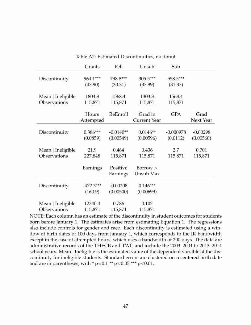
Table A2: Estimated Discontinuities, no donut
Grants Pell Unsub Sub
Discontinuity 964.1*** 798.8*** 305.5*** 558.5***(43.90) (30.31) (37.99) (31.37)
Mean | Ineligible 1804.8 1568.4 1303.3 1568.4Observations 115,871 115,871 115,871 115,871
Hours ReEnroll Grad in GPA GradAttempted Current Year Next Year
Discontinuity 0.386*** -0.0140** 0.0146** -0.000978 -0.00298(0.0859) (0.00549) (0.00596) (0.0112) (0.00560)
Mean | Ineligible 21.9 0.464 0.436 2.7 0.701Observations 227,848 115,871 115,871 115,871 115,871
Earnings Positive Borrow >Earnings Unsub Max
Discontinuity -472.3*** -0.00208 0.146***(160.9) (0.00500) (0.00699)
Mean | Ineligible 12340.4 0.786 0.102Observations 115,871 115,871 115,871
NOTE: Each column has an estimate of the discontinuity in student outcomes for studentsborn before January 1. The estimates arise from estimating Equation 1. The regressionsalso include controls for gender and race. Each discontinuity is estimated using a win-dow of birth dates of 100 days from January 1, which corresponds to the IK bandwidthexcept in the case of attempted hours, which uses a bandwidth of 200 days. The data areadministrative records of the THECB and TWC and include the 2003–2004 to 2013–2014school years. Mean | Ineligible is the estimated value of the dependent variable at the dis-continuity for ineligible students. Standard errors are clustered on recentered birth dateand are in parentheses, with * p<0.1 ** p<0.05 *** p<0.01.
47

Table A3: Covariate Balance
Male White Black Hispanic Asian PreviousGrants
Discontinuity -0.00104 -0.00154 0.000446 0.00938 -0.00552** 16.80(0.00667) (0.00706) (0.00384) (0.00613) (0.00280) 36.04
Mean | Ineligible 0.484 0.483 0.107 0.3 0.0494 1828.8
Observations 111,795 111,795 111,795 111,795 111,795 111,795
SAT ACT Top 10 Top Previous Previous Previous11-25 EFC Student AGI Parent AGI
Discontinuity 1.242 -0.0572 0.00609 -0.00492 -51.13 -15.70 -62.62(5.259) (0.173) (0.00423) (0.00412) (194.5) (247.1) (3694.1)
Mean | Ineligible 1005.9 20.45 0.0926 0.0935 7095.5 7841.8 66088.5
Observations 21,017 10,332 85,413 85,413 64,134 34,892 35,614NOTE: This tests for discontinuities in covariates for students who were born before January 1. Each discontinuity isestimated using a window of birth dates of 100 days from January 1 which corresponds to the IK bandwith. Students bornDecember 29 through January 3 are excluded as discussed in the text. The data are administrative records of the THECBand include the 2002–2003 to 2013–2014 school years. Mean | Ineligible is the estimated value of the dependent variableat the discontinuity for ineligible students. Standard errors are clustered on birthdate are in parentheses, with * p<0.1 **p<0.05 *** p<0.01.
48
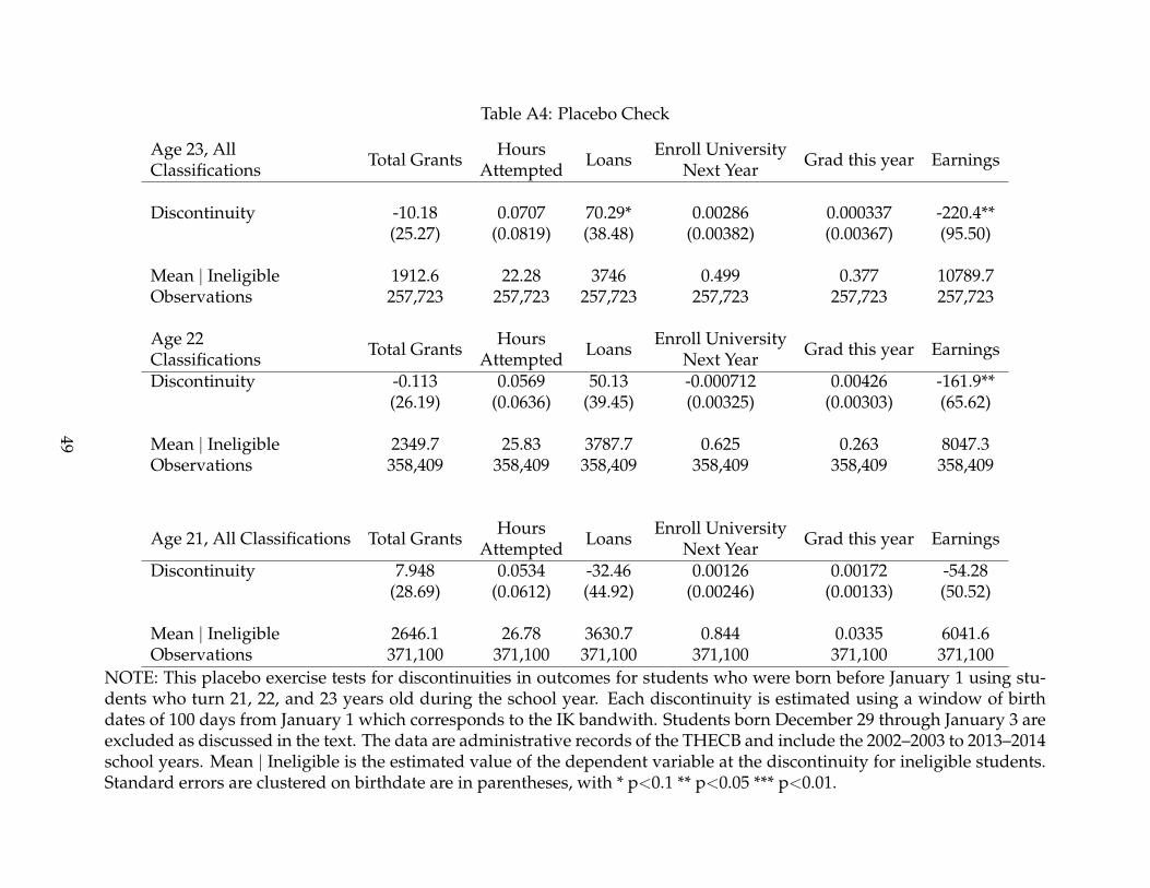
Table A4: Placebo Check
Age 23, AllClassifications Total Grants Hours
Attempted Loans Enroll UniversityNext Year Grad this year Earnings
Discontinuity -10.18 0.0707 70.29* 0.00286 0.000337 -220.4**(25.27) (0.0819) (38.48) (0.00382) (0.00367) (95.50)
Mean | Ineligible 1912.6 22.28 3746 0.499 0.377 10789.7Observations 257,723 257,723 257,723 257,723 257,723 257,723
Age 22Classifications Total Grants Hours
Attempted Loans Enroll UniversityNext Year Grad this year Earnings
Discontinuity -0.113 0.0569 50.13 -0.000712 0.00426 -161.9**(26.19) (0.0636) (39.45) (0.00325) (0.00303) (65.62)
Mean | Ineligible 2349.7 25.83 3787.7 0.625 0.263 8047.3Observations 358,409 358,409 358,409 358,409 358,409 358,409
Age 21, All Classifications Total Grants HoursAttempted Loans Enroll University
Next Year Grad this year Earnings
Discontinuity 7.948 0.0534 -32.46 0.00126 0.00172 -54.28(28.69) (0.0612) (44.92) (0.00246) (0.00133) (50.52)
Mean | Ineligible 2646.1 26.78 3630.7 0.844 0.0335 6041.6Observations 371,100 371,100 371,100 371,100 371,100 371,100
NOTE: This placebo exercise tests for discontinuities in outcomes for students who were born before January 1 using stu-dents who turn 21, 22, and 23 years old during the school year. Each discontinuity is estimated using a window of birthdates of 100 days from January 1 which corresponds to the IK bandwith. Students born December 29 through January 3 areexcluded as discussed in the text. The data are administrative records of the THECB and include the 2002–2003 to 2013–2014school years. Mean | Ineligible is the estimated value of the dependent variable at the discontinuity for ineligible students.Standard errors are clustered on birthdate are in parentheses, with * p<0.1 ** p<0.05 *** p<0.01.
49
Related Documents


