Distributional effects of non-cash incomes in seven European countries

Panos Tsakloglou,1 Tim Callan,2 Kieran Coleman,2 Conchita D'Ambrosio,3 Klaas de Vos,4 Joachim R. Frick,5 Chiara Gigliarano,6 Tim Goedemé,7

Markus M. Grabka,5 Olaf Groh-Samberg,5 Claire Keane,2 Christos Koutsambelas,1 Stijn Lefebure,7 Mattia Makovec,8 Killian Mullan,9 Tim Smeeding,10

Holly Sutherland,9 Gerlinde Verbist,7 and Francesca Zantomio9

Distributional effects of non-cash incomes in seven European countries

AIM-AP Project 1 – Comparative Report

January 2009

1 Athens University of Economics and Business and CERES 2 ESRI, Dublin

3 Università di Milano-Bicocca and DIW, Berlin 4 CentERdata, Tilburg University

5 DIW Berlin 6 Università Politecnica delle Marche, Ancona

7 Centre for Social Policy Herman Deleeck, University of Antwerp 8 Universidad de Chile

9 Institute for Social and Economic Research, University of Essex 10 Luxembourg Income Study and University of Wisconsin-Madison

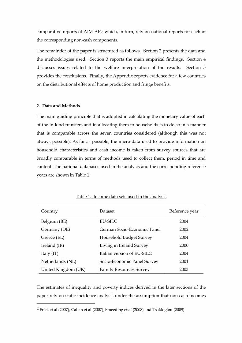
Abstract

Most empirical distributional studies in developed countries rely on distributions of

disposable income. From a theoretical point of view this practice is contentious since

a household‟s command over resources is determined not only by its spending

power over commodities it can buy in the market but also on resources available to

the household members through non-market mechanisms such as the in-kind

provisions of the welfare state and the use of private non-cash incomes. The present

paper examines the combined effects of including three of the most important non-

cash incomes enjoyed by private households in the concept of resources in seven

European countries (Belgium, Germany, Greece, Italy, Ireland, the Netherlands and

the UK). These non-cash incomes are imputed rent, public education services and

public health care services. Further, limited evidence is presented on the likely

distributional effects of home production and fringe benefits. The empirical results

show that, in a framework of static incidence analysis, the inclusion of these non-cash

income components in the concept of resources leads to a substantial decline in the

measured levels of inequality and poverty. The main beneficiaries appear to be

elderly individuals and, to a lesser extent, households with children. Nevertheless,

the inclusion of non-cash incomes in the concept of resources does not lead to either

substantial change in the ranking of the countries according to their level of

inequality or significant changes in the structure of inequality. The welfare

interpretation of some of the findings is not straightforward, especially regarding the

universally provided public health and education services that have a strong life-

cycle pattern. If adjustments are made to the equivalence scales used in the analysis

to take account of differences in needs for health and education services, the

distributional effects of these transfers appear to be far more modest.

1. Introduction

The great majority of empirical studies analyzing cross-national differences in the

levels of inequality and poverty as well as the redistributive effectiveness of welfare

state policies utilize data on the disposable income of the population members. Such

studies focusing in Europe tend to confirm hypotheses about distinct welfare state

regimes in particular sets of countries [Titmus (1958), Esping-Andersen (1990),

Ferrera (1996)] and emphasize the importance of welfare state transfers, particularly

for those segments of the population located close to the bottom of the income

distribution. Scandinavian and Nordic countries are big spenders and reduce

inequality the most; the English speaking countries spend relatively little and reduce

inequality the least; and the continental European countries spend a lot, but achieve

less equality than the Scandinavians. Southern European nations spend the least and

have the highest inequality and poverty [Atkinson et al (1995), Gustafsson and

Johansson (1999), Heady, Mitrakos and Tsakloglou (2001), Alderson and Nielsen

(2002), Dennis and Guio (2003), Moller et al (2003), Kenworthy (2004), Förster and

Mira d'Ercole (2004), Hacker et al (2005)].

Nevertheless, in the developed countries, about half of welfare state transfers consist

of in kind benefits such as education, health insurance, child care, elderly care and

other services. In kind as well as cash transfers reduce inequalities in standards of

living as documented in research within selected countries but only occasionally

cross nationally and never for a large set of rich countries [for notable exceptions, see

Smeeding et al (1993) and Marical et al (2006)]. The theoretical and empirical

importance of valuing in kind benefits has been understood for a long time

[Smeeding (1977, 1982)]. Conceptually it is clear that these benefits are worth some

nontrivial amount to beneficiaries. Therefore, from a theoretical point of view, a

measure that counts in kind transfers is superior to the conventional measure of cash

disposable income as a measure of a household‟s standard of living [Atkinson and

Bourguignon (2000), Atkinson et al (2002), Canberra Group (2001)].

Besides publicly provided in-kind transfers, there are also substantial private non-

cash incomes. The most well known is, probably, imputed rent for owner occupied

accommodation. Of lesser importance for developed market economies but of great

significance in many developing countries, particularly those with large agricultural

sectors, are commodities produced for own consumption or barter without the

intervention of the market mechanism. Finally, for an evaluation of the full concept

of resources available to the household, one should also take into account home

produced and consumed services.

The omission of non-cash incomes from the concept of resources used in

distributional studies may call into question the validity of several comparisons of

distributional outcomes of these studies - both time-series within a particular country

and cross-sectional across countries. For example, inter-temporal comparisons of

inequality or poverty in a particular country ignoring publicly provided services in

general are likely to lead to misleading conclusions at times of considerable

expansion or contraction of the role of the welfare state. Likewise, comparisons of

inequality and poverty levels between groups of countries with dramatically

different welfare state arrangements regarding the provision of particular services

may well lead to erroneous conclusions. For instance, comparing the income

distributions of two countries, one where health services are primarily covered by

private out-of-pocket payments and another where such services are provided free of

charge by the state to the citizens is likely to lead to invalid conclusions and, perhaps,

policy implications.

Existing empirical studies of the distributional effects of both publicly provided and

private non-cash incomes using a variety of imputation methods and national or

cross-country data sets covering developed countries tend to confirm that non-cash

incomes are more equally distributed than monetary incomes.1 The aim of the

present paper is to analyse in detail the aggregate combined distributional effects of

imputed rent, public education services and public health care services using

common methodologies in roughly similar data sets of seven European countries

(Belgium, Germany, Greece, Ireland, Italy, the Netherlands and the United

Kingdom). Some indications of the likely distributional effects of home production

and fringe benefits are given in an appendix. It relies on the four corresponding

1 See, for example, O‟Higgins and Ruggles (1981), Bryant and Zick (1985), James and Benjamin (1987), Lampman (1988), Smeeding et al (1993), Evandrou et al (1993), Meulemans and Cantillon (1993), Yates (1994), Whiteford and Kennedy (1995), McLennan (1996), Steckmest (1996), Jenkins and O‟Leary (1996), Huguenenq (1998), Tsakloglou and Antoninis (1999), Harris (1999), Antoninis and Tsakloglou (2001), Pierce (2001), Sefton (2002), Frick and Grabka (2003), Chung (2003), Saunders and Siminski (2004), Lakin (2004), Caussat et al. (2005), Aaberge et al. (2006), Harding, Lloyd and Warren (2006), Garfinkel et al (2006), Marical et al (2006), Wolff and Zacharias (2006), Frazis and Stewart (2009)

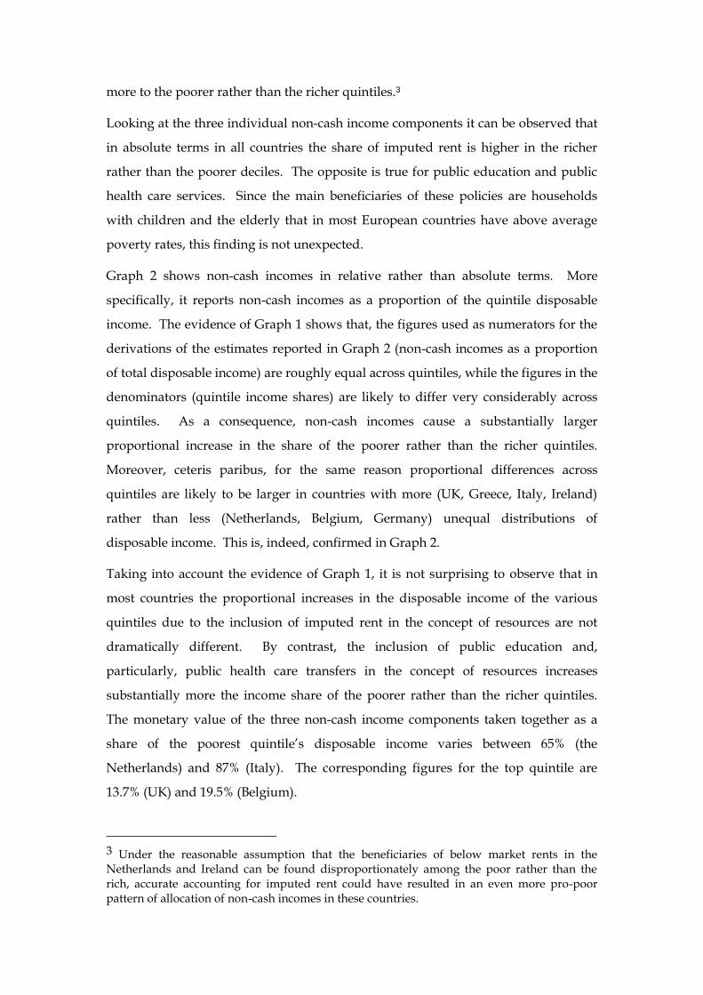
comparative reports of AIM-AP,2 which, in turn, rely on national reports for each of

the corresponding non-cash components.

The remainder of the paper is structured as follows. Section 2 presents the data and

the methodologies used. Section 3 reports the main empirical findings. Section 4

discusses issues related to the welfare interpretation of the results. Section 5

provides the conclusions. Finally, the Appendix reports evidence for a few countries

on the distributional effects of home production and fringe benefits.

2. Data and Methods

The main guiding principle that is adopted in calculating the monetary value of each

of the in-kind transfers and in allocating them to households is to do so in a manner

that is comparable across the seven countries considered (although this was not

always possible). As far as possible, the micro-data used to provide information on

household characteristics and cash income is taken from survey sources that are

broadly comparable in terms of methods used to collect them, period in time and

content. The national databases used in the analysis and the corresponding reference

years are shown in Table 1.

Table 1. Income data sets used in the analysis

Country Dataset Reference year

Belgium (BE) EU-SILC 2004

Germany (DE) German Socio-Economic Panel 2002

Greece (EL) Household Budget Survey 2004

Ireland (IR) Living in Ireland Survey 2000

Italy (IT) Italian version of EU-SILC 2004

Netherlands (NL) Socio-Economic Panel Survey 2001

United Kingdom (UK) Family Resources Survey 2003

The estimates of inequality and poverty indices derived in the later sections of the

paper rely on static incidence analysis under the assumption that non-cash incomes

2 Frick et al (2007), Callan et al (2007), Smeeding et al (2008) and Tsakloglou (2009).

(and, in particular, public transfers in-kind) do not create externalities. No dynamic

effects are considered in the present analysis. In other words, it is assumed that the

recipients of these incomes and the members of their households are the sole

beneficiaries and that these non-cash income components do not create any benefits

or losses to the non-recipients. Moreover, in the cases of public education and public

health care it is assumed that the value of the transfer to the beneficiary is equal to

the average cost of producing the corresponding services. Similar assumptions are

standard practice in the analysis of the distributional impact of publicly provided

services [Smeeding et al (1993), Marical et al (2006)]. The following paragraphs

describe briefly how the estimates of non-cash income were derived for each of the

three components (imputed rent, public education and public health care).

Following the EU Commission regulation (EC) No. 1980/2003 imputed rent is

defined as follows: “The imputed rent refers to the value that shall be imputed for all

households that do not report paying full rent, either because they are owner-occupiers or they

live in accommodation rented at a lower price than the market price, or because the

accommodation is provided rent-free. The imputed rent shall be estimated only for those

dwellings (and any associated buildings such a garage) used as a main residence by the

households. The value to impute shall be the equivalent market rent that would be paid for a

similar dwelling as that occupied, less any rent actually paid (in the case where the

accommodation is rented at a lower price than the market price), less any subsidies received

from the government or from a non-profit institution (if owner-occupied or the

accommodation is rented at a lower price than the market price), less any minor repairs or

refurbishment expenditure which the owner-occupier households make on the property of the

type that would normally be carried out by landlords. The market rent is the rent due for the

right to use an unfurnished dwelling on the private market, excluding charges for heating,

water, electricity, etc.”

Due to data limitations, it was not possible to apply the same methodology to all

seven countries involved in the project. In five of them (Belgium, Germany, Greece,

Italy and UK) the “rental equivalence” (or, “opportunity cost”) method was applied.

There are three stages in its implementation. First, a regression model is estimated

with rent (per square meter) as dependent variable based on the population of

tenants in the private, non-subsidized market, while the explanatory variables

include a wide range of characteristics of the dwelling, occupancy, and so on. Then,

the resulting coefficients are applied to otherwise similar owner-occupiers and

tenants paying below-market rent. The estimates thus derived refer to the gross

imputed rent. Finally, in order to derive estimates of the net imputed rent that can be

used for cross-country comparisons, mortgage interest payments (in the case of

owner occupiers and actual rent paid (in the case of tenants paying below market

rent) and operating and maintenance costs (for both groups) are subtracted from the

gross imputed rent estimate.

In the datasets used in the cases of Ireland and the Netherlands, insufficient

information on (market) rents of tenant households was available and, hence, the

above method could not be applied. However, in both data sets self-reported

information was available on the market value of the accommodation as well as

mortgage interest payments and maintenance costs. Therefore, estimates of imputed

rent were derived using an alternative method, the “capital market approach”. More

specifically, estimates of the gross imputed rent were derived by applying a country-

specific interest rate to the market value of the accommodation and the

corresponding housing specific costs were subtracted in order to derive estimates of

the net imputed rent. Unfortunately, this implies that there is no imputed rent

measure for (subsidized) tenants in those two countries which clearly reduces cross-

country comparability of the distributional effects of imputed rent.

Regarding education, information on spending per student in primary, secondary

and tertiary education is derived from OECD‟s “Education at a glance 2006”. Each

student in a public education institution (or a heavily subsidized private education

institution) identified in the income survey was assigned a public education transfer

equal to the average cost of producing these services in the corresponding level of

education. Then, this benefit was assumed to be shared by all household members.

In other words, it was implicitly assumed that in the absence of public transfers the

students and their families would have to undertake the expenditures themselves.

Because of limitations on the information available on education in some of the

income surveys we focus on three levels of education (primary, secondary and

tertiary), thus leaving aside other levels such as pre-primary and non-tertiary post-

secondary education and suppressing distinctions, such as those between general

and technical secondary education, as well as Type A and Type B tertiary education

which may be important in some countries. R&D expenditures are not included in

the benefit received by tertiary education students, since it is assumed that the

students are not the primary beneficiaries of this type of public spending.

Estimates of public spending per student in primary, secondary and tertiary public

education institutions were derived as follows. Figures from Table X2.5 (p. 434) of

OECD‟s “Education at a glance 2006” (Annual expenditure on educational institutions

per student for all services (2003) in equivalent euros converted using PPP, by level of

education based on full-time equivalents) were multiplied by the estimates of the share of

public expenditures in total educational expenditures (separately for tertiary and

non-tertiary education) reported in Table B2.1b (p. 206) (Expenditure on educational

institutions as a percentage of GDP by level of education (1995, 2000, 2003) from public and

private sources by source of funds and year) and euro PPP conversion rates as reported in

Table X2.2 (p. 431) (Basic reference statistics (reference period: calendar year 2003, 2003

current prices). Then, in order to derive the corresponding estimates for years other

than 2003, these estimates were inflated or deflated using country specific nominal

GDP per capita conversion factors derived from the data of the on-line OECD

database (using real GDP growth rates, GDP deflators and population growth rates).

With respect to public health care services, the risk-related “insurance value

approach” was adopted. More specifically, the „insurance value‟ is the amount that

an insured person would have to pay in each category (in our case, narrowly defined

age group) so that the third party provider (government, employer, other insurer)

would have just enough revenue to cover all claims for such persons. It is based on

the notion that what the public health care services provided is equivalent to funding

an insurance policy where the value of the premium is the same for everybody

sharing the same characteristics, such as age. Then, this value is added to the

resources of each individual belonging to a particular group with the predefined

characteristic(s) and, correspondingly to his/her household.

We calculated per capita expenditures for each age group using the OECD Social

Expenditure database (SOCX), which provides data that are comparable across

countries. The health care expenditures are taken from the OECD Health Data and

include all public expenditure on health care, including among other things,

expenditure on in-patient care, ambulatory medical services, pharmaceutical goods

and prevention. They do not include non-reimbursed individual health expenditures

or cash benefits related to sickness [OECD (2007)]. One restriction of the SOCX

database arises from the fact that existing differences in the use of for health care

between men and women are not considered and there is evidence that spending

patterns differ across sexes [Costello and Bains (2001), Carone et al (2005)]. Another

restriction is that “research and development” (R&D) spending is included, since it

may be argued that this component is not relevant for current welfare. The SOCX

database does not allow the deduction of this component.

For the purposes of the empirical analysis, the non-cash income components are

added to the concept of resources of the baseline distribution (distribution of

disposable monetary income) and comparisons are made. In order to take into

account household economies of scale and differences in needs between adults and

children, in both cases, the total household resources are divided by the household

equivalence scale and the resulting figure is assigned to all household members.

Following EUROSTAT, in the next section the equivalence scales used assign weight

of 1.00, 0.50 and 0.30 to the household head, each of the remaining adults and each

child in the household, respectively.

Table 2. Non-cash income components as a proportion of total disposable income

Country Imputed

Rent Public

Education Public

Health Care All

Belgium (BE) 6.0 13.2 16.3 35.5

Germany (DE) 7.2 7.2 16.5 30.9

Greece (EL) 11.1 7.2 10.3 28.6

Ireland (IR) 9.3 11.9 12.2 33.4

Italy (IT) 10.6 9.5 13.7 33.8

Netherlands (NL) 6.1 10.6 11.2 27.9

United Kingdom (UK) 7.9 10.2 12.7 30.8

3. Empirical results

Table 2 reports the monetary value of the three non-cash income components as a

proportion of the total disposable income of the population in the seven countries

under consideration. As noted above, the estimates of imputed rent for Ireland and

the Netherlands are not strictly comparable with those of the other countries and,

hence, are reported in italics. The figures for these countries underestimate the true

value of imputed rent and, hence, its share as a proportion of disposable monetary

income. Looking at the individual non-cash incomes, cross-country differences are

substantial. They can be attributed to a variety of reasons. In the case of imputed

rent, it seems that the main determinant is likely to be the extent of homeownership

and, particularly, outright home ownership. In the cases of public education and

public health care, the demographic structure of the population is likely to be an

important determinant; ceteris paribus, countries with younger/older populations

are likely to spend more in education/health. Moreover, in these cases, cross-

country differences in the importance of private out-of-pocket payments for

obtaining education and health services can account for a considerable proportion of

cross-country differences.

In the countries under consideration imputed rent is equivalent to between 6.0% and

11.1% of disposable income. The corresponding ranges for public education and

public health care are 7.2%-13.2% and 10.3%-16.5%. When the three non-cash

incomes are put together, cross country differences are still relatively large, but not

very substantial. In Greece and the Netherlands they add up to around 28% of

disposable income, in Germany and the UK a little below 31%, in Ireland and Italy a

little above 33% and in Belgium 35.5%.

For the purposes of our analysis, what is equally, if not even more, important is the

distribution of the non-cash incomes across the distribution of income. Graph 1

provides a picture of the distribution of non-cash income components across

quintiles, when the members of the population are grouped according to their

equivalised disposable income. The pattern is relatively similar across countries.

Non-cash incomes appear to be fairly evenly distributed across quintiles, at least in

four of the countries examined here (Belgium, Germany, Greece and Italy). In the

Netherlands and, to a lesser extent, in the UK and Ireland non-cash incomes accrue

Graph 1. Distribution of non-cash income components across quintiles

(as % of total monetary income)

0

2

4

6

8

1 2 3 4 5

Belgium

0

2

4

6

8

1 2 3 4 5

Germany

0

2

4

6

8

1 2 3 4 5

Greece

0

2

4

6

8

1 2 3 4 5

Ireland

0

2

4

6

8

1 2 3 4 5

Italy

0

2

4

6

8

1 2 3 4 5

Netherlands

0

2

4

6

8

1 2 3 4 5

UK

Public Health Care

Public Education

Imputed Rent

more to the poorer rather than the richer quintiles.3

Looking at the three individual non-cash income components it can be observed that

in absolute terms in all countries the share of imputed rent is higher in the richer

rather than the poorer deciles. The opposite is true for public education and public

health care services. Since the main beneficiaries of these policies are households

with children and the elderly that in most European countries have above average

poverty rates, this finding is not unexpected.

Graph 2 shows non-cash incomes in relative rather than absolute terms. More

specifically, it reports non-cash incomes as a proportion of the quintile disposable

income. The evidence of Graph 1 shows that, the figures used as numerators for the

derivations of the estimates reported in Graph 2 (non-cash incomes as a proportion

of total disposable income) are roughly equal across quintiles, while the figures in the

denominators (quintile income shares) are likely to differ very considerably across

quintiles. As a consequence, non-cash incomes cause a substantially larger

proportional increase in the share of the poorer rather than the richer quintiles.

Moreover, ceteris paribus, for the same reason proportional differences across

quintiles are likely to be larger in countries with more (UK, Greece, Italy, Ireland)

rather than less (Netherlands, Belgium, Germany) unequal distributions of

disposable income. This is, indeed, confirmed in Graph 2.

Taking into account the evidence of Graph 1, it is not surprising to observe that in

most countries the proportional increases in the disposable income of the various

quintiles due to the inclusion of imputed rent in the concept of resources are not

dramatically different. By contrast, the inclusion of public education and,

particularly, public health care transfers in the concept of resources increases

substantially more the income share of the poorer rather than the richer quintiles.

The monetary value of the three non-cash income components taken together as a

share of the poorest quintile‟s disposable income varies between 65% (the

Netherlands) and 87% (Italy). The corresponding figures for the top quintile are

13.7% (UK) and 19.5% (Belgium).

3 Under the reasonable assumption that the beneficiaries of below market rents in the Netherlands and Ireland can be found disproportionately among the poor rather than the rich, accurate accounting for imputed rent could have resulted in an even more pro-poor pattern of allocation of non-cash incomes in these countries.

Graph 2. Non-cash income components as a proportion of the disposable income of quintiles

0

20

40

60

80

100

1 2 3 4 5

Belgium

0

20

40

60

80

100

1 2 3 4 5

Germany

0

20

40

60

80

100

1 2 3 4 5

Greece

0

20

40

60

80

100

1 2 3 4 5

Ireland

0

20

40

60

80

100

1 2 3 4 5

Italy

0

20

40

60

80

100

1 2 3 4 5

Netherlands

0

20

40

60

80

100

1 2 3 4 5

UK

Health

Education

Imputed Rent

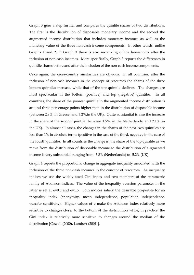
Graph 3 goes a step further and compares the quintile shares of two distributions.

The first is the distribution of disposable monetary income and the second the

augmented income distribution that includes monetary incomes as well as the

monetary value of the three non-cash income components. In other words, unlike

Graphs 1 and 2, in Graph 3 there is also re-ranking of the households after the

inclusion of non-cash incomes. More specifically, Graph 3 reports the differences in

quintile shares before and after the inclusion of the non-cash income components.

Once again, the cross-country similarities are obvious. In all countries, after the

inclusion of non-cash incomes in the concept of resources the shares of the three

bottom quintiles increase, while that of the top quintile declines. The changes are

most spectacular in the bottom (positive) and top (negative) quintiles. In all

countries, the share of the poorest quintile in the augmented income distribution is

around three percentage points higher than in the distribution of disposable income

(between 2.8%, in Greece, and 3.2%,in the UK). Quite substantial is also the increase

in the share of the second quintile (between 1.5%, in the Netherlands, and 2.1%, in

the UK). In almost all cases, the changes in the shares of the next two quintiles are

less than 1% in absolute terms (positive in the case of the third, negative in the case of

the fourth quintile). In all countries the change in the share of the top quintile as we

move from the distribution of disposable income to the distribution of augmented

income is very substantial, ranging from -3.8% (Netherlands) to -5.2% (UK).

Graph 4 reports the proportional change in aggregate inequality associated with the

inclusion of the three non-cash incomes in the concept of resources. As inequality

indices we use the widely used Gini index and two members of the parametric

family of Atkinson indices. The value of the inequality aversion parameter in the

latter is set at e=0.5 and e=1.5. Both indices satisfy the desirable properties for an

inequality index (anonymity, mean independence, population independence,

transfer sensitivity). Higher values of e make the Atkinson index relatively more

sensitive to changes closer to the bottom of the distribution while, in practice, the

Gini index is relatively more sensitive to changes around the median of the

distribution [Cowell (2000), Lambert (2001)].

Graph 3. Differences in quintile income shares between monetary and augmented income distributions

-6

-5

-4

-3

-2

-1

0

1

2

3

4

1 2 3 4 5

Belgium

-6

-5

-4

-3

-2

-1

0

1

2

3

4

1 2 3 4 5

Germany

-6

-5

-4

-3

-2

-1

0

1

2

3

4

1 2 3 4 5

Greece

-6

-5

-4

-3

-2

-1

0

1

2

3

4

1 2 3 4 5

Ireland

-6

-5

-4

-3

-2

-1

0

1

2

3

4

1 2 3 4 5

Italy

-6

-5

-4

-3

-2

-1

0

1

2

3

4

1 2 3 4 5

Netherlands

-6

-5

-4

-3

-2

-1

0

1

2

3

4

1 2 3 4 5

UK

Graph 4. Proportional changes in inequality after the inclusion of non-cash income components in the concept of resources

The evidence of Graph 4 illustrates very clearly that in all countries under

examination, the inclusion of non-cash incomes in the concept of resources reduces

the values of the indices very substantially. In all cases the recorded effects are larger

when the Atkinson index is used, particularly for higher values of the inequality

aversion parameter. The proportional changes are relatively larger in Belgium, UK,

Netherlands and Ireland. The value of the Gini index declines between -19.3%

(Greece) and -23.3% (UK), while the corresponding proportional decline in the value

of A0.5 is between -35.0% (Greece) and 40.5% (UK) and in the value of A1.5 between

-37.0% (Greece) and -53.6% (Belgium).

Graph 5 is the counterpart of Graph 4 for changes in relative poverty after the

inclusion of non-cash incomes in the concept of resources. Following EUROSTAT,

the poverty line is drawn at the level of 60% of the median of the corresponding

distribution. The poverty indices used belong to the parametric family of Foster et al

(1984) (FGT). When the value of the poverty aversion parameter is set at a=0, the

index becomes the widely used “head count” poverty rate, that is the share of the

population falling below the poverty line. When a=1, the index becomes the

normalized income gap ratio, while when a=2 the index satisfies the axioms

proposed by Sen (1976) (anonymity, focus, monotonicity and transfer sensitivity) and

-60

-50

-40

-30

-20

-10

0

BE DE EL IR IT NL UK

Gini

Atkinson0.5

Atkinson1.5

is sensitive not only to the population share of the poor and their average poverty

gap, but also to the inequality in the distribution of resources among the poor.

Graph 5. Proportional changes in poverty after the inclusion of non-cash income

components in the concept of resources

The proportional changes reported in Graph 5 are even larger than those reported in

Graph 4 and, in all cases, the larger the value of the poverty aversion parameter the

larger the recorded decline in relative poverty. The poverty rate (FGT0) declines

between -37.7% (Italy) and -55.9% (Netherlands), the normalised income gap ration

(FGT1) between -53.1% (Italy) and -61.6% (Ireland), while FGT2 declines between -

64.5% (Belgium) and -71.8% (Greece).

Do the changes reported in Graphs 4 and 5 lead to a re-ranking of the countries

regarding their levels of inequality and poverty? An attempt to answer this question

is provided in Table 3. Starting from the upper half of the table, it can be noted that

no re-ranking is taking place regarding the two countries with the lowest level of

inequality (Belgium and the Netherlands). Re-ranking is observed among countries

with medium or high levels of inequality. However, even in this case the re-ranking

is not very substantial, with countries moving only one rank up or down in the

distribution of augmented income vis-à-vis their rank in the distribution of

-80

-70

-60

-50

-40

-30

-20

-10

0

BE DE EL IR IT NL UK

FGT0

FGT1

FGT2

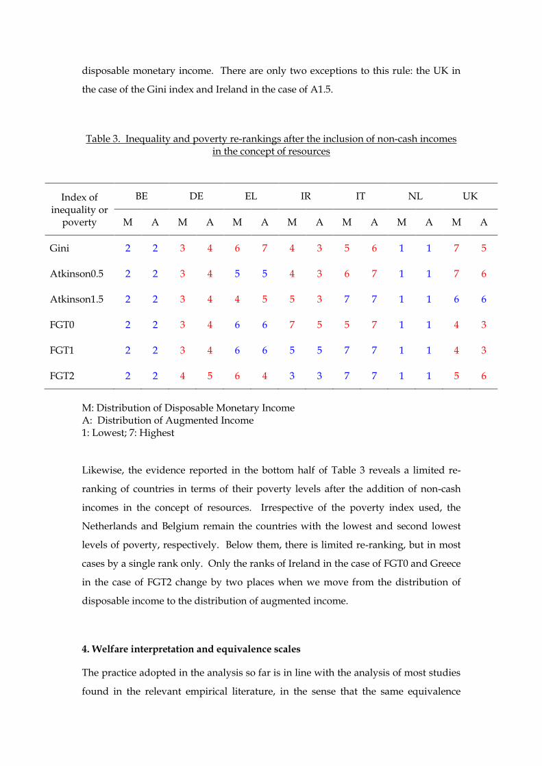
disposable monetary income. There are only two exceptions to this rule: the UK in

the case of the Gini index and Ireland in the case of A1.5.

Table 3. Inequality and poverty re-rankings after the inclusion of non-cash incomes in the concept of resources

Index of inequality or

poverty

BE DE EL IR IT NL UK

M A M A M A M A M A M A M A

Gini 2 2 3 4 6 7 4 3 5 6 1 1 7 5

Atkinson0.5 2 2 3 4 5 5 4 3 6 7 1 1 7 6

Atkinson1.5 2 2 3 4 4 5 5 3 7 7 1 1 6 6

FGT0 2 2 3 4 6 6 7 5 5 7 1 1 4 3

FGT1 2 2 3 4 6 6 5 5 7 7 1 1 4 3

FGT2 2 2 4 5 6 4 3 3 7 7 1 1 5 6

M: Distribution of Disposable Monetary Income A: Distribution of Augmented Income 1: Lowest; 7: Highest Likewise, the evidence reported in the bottom half of Table 3 reveals a limited re-

ranking of countries in terms of their poverty levels after the addition of non-cash

incomes in the concept of resources. Irrespective of the poverty index used, the

Netherlands and Belgium remain the countries with the lowest and second lowest

levels of poverty, respectively. Below them, there is limited re-ranking, but in most

cases by a single rank only. Only the ranks of Ireland in the case of FGT0 and Greece

in the case of FGT2 change by two places when we move from the distribution of

disposable income to the distribution of augmented income.

4. Welfare interpretation and equivalence scales

The practice adopted in the analysis so far is in line with the analysis of most studies

found in the relevant empirical literature, in the sense that the same equivalence

scales – in our case the modified OECD scales used by EUROSTAT– are used for the

distribution of disposable income and for the distribution of augmented income. This

may be problematic, particularly in the case of the two largest universal non-cash

public transfers (public education and public health care) that are also characterized

by strong life-cycle patterns. The reason is that these scales are “conditional” on

existing external arrangements [Pollak and Wales (1979), Blundell and Lewbel (1991),

Radner (1997)]. In other words, they are conditional on the existence of free public

education and free public health care. By introducing the latter in the concept of

resources in the “augmented” income distribution, we treat them like private

commodities to which the households need to devote resources in order to obtain

them. Therefore, the equivalence scales should be modified accordingly. This

argument does not apply in the case of imputed rent (as well as home production

and fringe benefits).

The appropriate modification of the household equivalence scales used in the

analysis is not an easy task. Both education and health care have some rather unique

characteristics. Their consumption is absolutely necessary for the individuals

involved (arguably, more so for health) and their consumption does not involve any

economies of scale at the household level. Therefore, we should adopt a “fixed cost”

approach, assuming that the needs of the recipients of these services are equal to a

specific sum of money. For example, we can assume that the per capita amounts

spent by the state for age-specific population groups on public education and public

health care depict accurately the corresponding needs of these groups. Then, the re-

calculation of equivalence scales is easy, albeit in this case the effects of these public

transfers in kind on measured levels of inequality and poverty should be zero almost

by definition.

In general, assuming that y is household disposable income, k is the amount of extra

needs of the household members for health and education (or each of them

separately), e the OECD scale and e‟ the new scale, the following should be valid for

the household to remain at the same welfare level:

y/e = (y+k)/e‟

and e‟ should be equal to

e‟ = e(y+k)/y

Table 4a. Proportional changes in inequality indices as a result of public education transfers in-kind under alternative concepts of equiv. scales (under the assumption that only persons in compulsory education have education needs)

Belgium Germany Greece Italy UK

G A0.5 A1.5 G A0.5 A1.5 G A0.5 A1.5 G A0.5 A1.5 G A0.5 A1.5

Baseline -6.9 -12.7 -7.8 -7.4 -13.3 -12.1 -6.3 -13.4 -19.4 -9.2 -17.2 -19.0 -7.9 -13.8 -17.8

National -0.8 -2.2 -2.9 -1.8 -3.6 -3.8 -1.9 -3.8 -4.0 -1.8 -3.6 -4.7 -1.0 -2.3 -9.6

EU15 min -2.9 -5.9 -4.7 -3.2 -6.1 -6.2 -3.0 -6.0 -7.8 -4.7 -9.2 -10.8 -2.8 -5.4 -12.1

EU15 average -0.7 -1.9 -2.7 -1.4 -2.7 -2.9 -1.7 -3.4 -3.6 -2.9 -5.8 -7.1 -0.6 -1.6 -9.0

EU15 max 2.0 2.9 -0.3 0.5 0.9 0.6 -0.5 -0.8 0.4 -1.2 -2.5 -3.4 1.5 2.3 -5.7

Table 4b. Proportional changes in inequality indices as a result of public education transfers in-kind under alternative concepts of equiv. scales

(under the assumption that all students have education needs)

Belgium Germany Greece Italy UK

G A0.5 A1.5 G A0.5 A1.5 G A0.5 A1.5 G A0.5 A1.5 G A0.5 A1.5

Baseline -6.9 -12.7 -7.8 -7.4 -13.3 -12.1 -6.3 -13.4 -19.4 -9.2 -17.2 -19.0 -7.9 -13.8 -17.8

National 0.0 0.0 0.0 0.0 0.0 0.0 -0.1 -0.1 0.2 0.0 0.0 0.0 0.2 0.4 0.3

EU15 min -2.5 -4.4 -2.6 -1.9 -3.6 -3.5 -1.3 -2.8 -3.9 -3.3 -6.3 -7.1 -2.0 -3.6 -4.8

EU15 average 0.1 0.3 0.2 0.5 0.9 0.9 0.5 1.1 1.6 -1.0 -1.9 -2.1 0.5 0.8 0.0

EU15 max 3.5 6.6 3.9 3.0 6.1 6.4 2.7 5.7 7.8 1.5 3.3 3.9 3.1 5.9 6.6

Table 5. Proportional changes in inequality indices as a result of public health care transfers in-kind under alternative concepts of equiv. scales

Belgium Germany Greece Italy UK

G A0.5 A1.5 G A0.5 A1.5 G A0.5 A1.5 G A0.5 A1.5 G A0.5 A1.5

Baseline -15.2 -28.9 -55.5 -13.4 -24.7 -25.6 -10.9 -21.4 -29.2 -11.8 -22.1 -28.2 -12.3 -22.0 -27.7

EU15 min -5.0 -9.3 -13.1 -6.3 -12.2 -12.6 -1.5 -3.0 -4.0 -4.0 -7.9 -9.6 -4.5 -8.4 -9.0

EU15 average 0.5 0.9 1.2 -2.3 -4.4 -4.5 3.1 6.3 7.6 0.3 0.5 0.6 -0.3 -0.5 -0.5

EU15 max 5.3 10.3 11.7 1.3 2.5 2.6 6.9 14.4 16.7 3.8 7.7 8.5 3.3 6.5 7.0

Naturally, there will be no single equivalence scale for households with identical

composition – the scale will be higher (smaller economies of scale) in poorer

households and lower (larger economies of scale) in better-off households. This is an

old postulate of equivalence scales theory that was long abandoned in favour of

simplicity and transparency (for comparative and policy purposes).

In democratic societies k and the level of the corresponding public provision is

determined through various forms of negotiation at several levels. It is not cast in

stone and may be affected by numerous factors such as the demographic

composition of the population, short- versus long-term considerations, etc.

Therefore, there is room for sensitivity analysis, using alternative values of k for

specific services (education, health care) and population groups (age specific

cohorts).

Then, there is the question of who has the corresponding needs. In the case of health

care the answer is clear: everybody has health care needs. Not so in the case of

education. Undoubtedly, students in compulsory levels of education have such

needs. Not necessarily so for students in non-compulsory levels that could have

participated in the labour market but opted to stay in the education system instead.

The implications of this alternative approach are explored in the following

paragraphs, exploiting cross-country variations in the level of provision of public

education and health care services as a share of GDP.

Table 4a – as well as the following two tables – is taken from Sutherland and

Tsakloglou (2009) and reports proportional changes in the three inequality indices

used in the paper (Gini, Atkinson(0.5) and Atkinson(1.5)) when public education

services are included in the concept of resources, using alternative equivalence

scales, in five of the countries included in the rest of the paper‟s analysis (all, apart

from Ireland and the Netherlands). For the purposes of this table it is assumed that

only students in ages corresponding to compulsory education have educational

needs. School leaving age varies in the five countries under consideration: 14.5 in

Greece, 15 in Italy, 16 in the UK, 18 in Belgium and Germany (OECD (2006) Education

at a Glance, Table C1.2). All persons below these age thresholds and above the

compulsory primary education enrolment age are considered to have educational

needs (including dropouts and private education students who do not receive any

public transfers), while the rest of the students in non-compulsory stages of the

education system may receive public transfers but are not assumed to have the

corresponding needs.

The first line of the table (“Baseline”) reports the proportional changes of the

inequality indices between the estimates derived from the distribution of disposable

income and the same distribution augmented by the value of in-kind public

education services using the modified OECD scales.4 The second line of the table

(“National”) reports estimates using different sets of equivalence scales for the two

distributions. More specifically, in this line it is assumed that in the case of the

augmented income distribution k is equal to the value provided by the state to

students in compulsory levels of education.

In the last three lines we exploit cross-country spending variations in EU15 and

adjust k accordingly. In these lines the value of k used in the second line is adjusted

in order to be equal as a share of GDP per capita to the minimum, (unweighted)

average and maximum of EU15 in the corresponding educational level using the

information of OECD (2006) Education at a Glance 2006, Table B1.4, p. 192 (“Annual

expenditure on educational institutions per student for all services relative to GDP

per capita”). The choice of EU15 is not accidental. All five countries considered here

are EU member-states and despite cross-country difference, in comparison with the

rest of the world, EU15 countries are pretty homogenous, fully-fledged democracies,

with relatively similar demographic structures and welfare state arrangements and

differences in their standards of living that are not enormous. Therefore, use of EU15

figures (as a share of GDP) can provide reasonable upper and lower bounds as well

as an average yardstick for our calculations. In this respect, cross-country variation

is considerable in EU15. The corresponding rates vary between 14-28%/19-35%/18-

46% of GDP per capita in the cases of primary/secondary/tertiary education, while

on average these percentages are 21%, 27% and 27%, for the three educational levels.

In most cases, spending per student as a share of GDP in the five countries under

consideration are close to the EU15 average, with the exception of Greece where the

corresponding figures are lower (especially regarding spending per student in

tertiary education).

4 These estimates are not strictly comparable to those used in the rest of the paper, since they have been derived using the disposable income distribution obtained from the simulation of the tax-benefit microsimulation model EUROMOD, rather than the income distributions of the datasets included in Table 1. The differences are very small, though.

As anticipated, in all countries the recorded proportional decline in inequality

between the distribution of cash disposable income and the augmented income

distribution is sharply reduced as we move from the first to the second line of the

table. Nevertheless, in all countries the aggregate result of these transfers remains

inequality-reducing. This should be attributed primarily to the transfers to

households with members in the non-compulsory stages of education (that are

assumed to receive transfers in-kind without having corresponding needs). In the

last three lines of the table recorded proportional reductions in inequality decline as

we move from the minimum to the maximum adjustment of needs for educational

services. In fact, when it is assumed that only students in compulsory education

have educational needs but the corresponding needs as a share of GDP per capita are

equal to the highest such figure in the EU15, the transition from the distribution of

cash disposable income to the augmented income distribution is associated with an

increase rather than a decline in inequality in most of the countries under

examination.

Table 4b is similar to Table 4a, but this time we assume that all students have needs

for education services, irrespective of their educational level, as do dropouts below

the official school leaving age of the country under consideration. Naturally, the first

line of the table is the same in both tables, while the second line records no changes

in recorded inequality in the three countries with limited information on students

below the official school leaving age (in other words, it is assumed that the persons

currently in education are compensated justly for their extra needs, which are

assumed to be equal to the corresponding state transfers per educational level). In

Greece and the UK, where detailed information is available for the type of school

attended by the student (public or private) as well as for his/her status as early

school leaver, the corresponding estimates are close to but not exactly zero. The two

forces are likely to operate in opposite directions. Since most private education

students are located close to the top of the distribution, the fact that they do not

receive a subsidy is likely to reduce recorded inequality. On the contrary, since most

dropouts are usually located close to the bottom of the distribution, the

corresponding lack of state transfers to them, despite their needs, is likely to lead to

increases in recorded inequality. The pattern in the last three lines of the table is

similar to the corresponding pattern of Table 4a but the differences across lines are

larger. More specifically, when it is assumed that the real needs of a student in a

particular educational level as a share of GDP per capita is equal to the minimum of

EU15 at this level (third line), educational transfers appear to reduce recorded

inequality – in other words, the households of the students are over-compensated

and since they are disproportionately located close to the bottom of the distribution,

these transfers appear to reduce inequality. Exactly the opposite is observed in the

last line of the table, where it is implicitly assumed that the students are

undercompensated for their extra educational needs. In the fourth line of the table,

where the corresponding needs are assumed to be equal to the EU15 average as a

share of GDP per capita, the recorded changes are small but regressive in all

countries apart from Italy. The result for Italy can be attributed to the fact that

according to this approach and the evidence reported in the aforementioned OECD

publication, Italy appears to overcompensate primary and, to a lesser extent,

secondary education students that are disproportionately represented in lower

income quintiles, while it undercompensates tertiary education students who are, in

most countries, more likely to be found in top quintiles.

Table 5 applies the same methodology to public health care transfers. No “National”

line appears in this table, since if it is assumed that all population members are justly

compensated for their extra health care needs, the result is distributionally neutral by

definition. If no adjustment is made to the equivalence scale, the reduction in the

recorded inequality is enormous and appears to be larger when inequality indices

sensitive to changes close to the bottom of the distribution are employed (such as

Atkinson (1.5)). However, this approach implicitly assumes that population

members with ill health are as equally well off as healthy population members with

similar levels of disposable income. In other words, this approach ignores that

health care needs are likely to be larger at particular life-stages. This inconsistency is

ameliorated in the last three lines of the table, where it is assumed that health care

needs vary according to the age of the population member. Taking as yardsticks the

lowest, average and highest health care spending per age group as a share of GDP,

the recorded changes in inequality are substantially lower. In fact, as anticipated, in

the last line the recorded changes in inequality are positive, and in some cases such

as Greece and Belgium quite substantial, while in the second line these transfers

appear to have a progressive impact only in the cases of Germany and (marginally)

the UK.

It is likely that the approach outlined above can contribute to a better understanding

of the distributional effects of non-cash public transfers. At this stage it may still be

relatively crude but can be improved in several ways. The two most promising

avenues are likely to be in the direction of uncovering variations in the quality of

services directed to particular segments of the population and the identification of

systematic under/over users of such services. For example, in countries with federal

rather than national education and/or health systems it may be possible to identify

regions with higher spending per capita (provided there is evidence that the higher

spending is translated in higher quality of services). In the case of education we can

identify persons who do not use public services such as private education students,

early school leavers, etc and, further we can bring pre-primary education into the

picture. In the case of health care we can differentiate between males and females,

identify private health insurance holders who may systematically underutilise the

public health care system or socioeconomic groups that, ceteris paribus, make

excessive use of the public services [Le Grand and Winter (1985)]. Likewise, we can

also identify persons with severe disabilities whose needs are likely to be higher than

the rest of the population (although they may also receive more expensive public

health care services).

5. Conclusions

The aim of the paper was to provide estimates of the distributional effects of three

large non-cash income components (imputed rent, public education and public

health care services) in seven European countries. In the countries under

examination – Belgium, Germany, Greece. Ireland, Italy, the Netherlands and the UK

– the total monetary value of these non-cash incomes is around one third of the

aggregate disposable income of the population. Using static incidence analysis,

under the assumption that incomes in-kind do not create externalities, it was shown

that non-cash incomes are far more equally distributed than cash incomes and, as a

result, their inclusion in the concept of resources leads to considerable reductions in

the measured levels of inequality and relative poverty. However, the relative

ranking of countries in terms of inequality and/or poverty indicators is affected only

marginally as we move from the distribution of disposable monetary income to the

augmented income distribution that includes cash as well as non-cash incomes.

Nevertheless, it was also pointed out that it is doubtful whether results derived using

the standard approach in the fields of public education and public health care can

have a straightforward welfare interpretation. The reason is that using this approach

we incorporate the value of the public services in the concept of household resources

but ignore the problem of extra needs of public services recipients. Once these needs

are taken into account with appropriate changes in the household equivalence scales

used in the analysis, the results regarding these non-cash income components appear

to be far more modest and, under particular circumstances may even appear to be

inequality-increasing.

REFERENCES

Aaberge R. and Langørgen A. (2006), “Measuring the Benefits from Public Services: The Effects of Local Government Spending on the Distribution of Income in Norway”, Review of Income and Wealth 52, pp. 61-83.

Alderson A.S. and Nielsen F (2002), “Globalization and the Great U-Turn: Income Inequality Trends in Sixteen OECD Countries”, American Journal of Sociology 107, pp. 1244-1299.

Antoninis M. and Tsakloglou P. (2001), “Who benefits from public education in Greece? Evidence and policy implications”, Education Economics 9, pp. 197-222.

Atkinson A.B. and Bourguignon F (2000), “Introduction: Income Distribution and Economics”, in A.B. Atkinson and F. Bourguignon (eds) Handbook of Income Distribution, Elvesier, Amsterdam and New York.

Atkinson A.B., Cantillon B., Marlier E. and Nolan B. (2002), Social indicators: The EU and social inclusion, Oxford University Press, Oxford.

Atkinson A.B., Rainwater M. and Smeeding T. (1995), Income distribution in OECD countries, Social Policy Studies No. 18, OECD, Paris.

Blundell R. and Lewbel A. (1991), "The information content of equivalence scales",

Journal of Econometrics 50, pp. 49-68.

Bryant W.K. and Zick C.D. (1985), “Income distribution implications of rural household production”, Journal of Agricultural Economics 67, pp. 1100-1104.

Callan T., Smeeding T. and Tsakloglou P. (2007), “Distributional effects of public education transfers in seven European countries”, AIM-AP report, University of Essex.

Canberra Group (2001), “Final Report and Recommendations”, The Canberra Group: Expert Group on Household Income Statistics, Ottawa.

Carone G., Costello D., Diez Guardia N., Mourre G., Przywara B. and Salomaki A. (2005), “The economic impact of ageing populations in the EU25 Member States”, European Economy 236.

Caussat L., Le Minez S. and Raynaud D. (2005), "L'assurance-maladie contribue-t-elle à redistribuer les revenus?", Drees, Dossiers solidarité et santé – Études sur les dépenses de santé, La Documentation Francaise, Paris.

Chung W. (2003), “Fringe benefits and inequality in the labor market”, Economic Inquiry 41, pp. 517-529.

Costello D. and Bains M. (2001), “Budgetary challenges posed by ageing populations”, Directorate General for Economic and Financial Affairs of the European Commission, Economic Policy Committee Document EPC/ECFIN/655/01-EN final.

Cowell F.A. (2000), “Measurement of inequality” in A.B. Atkinson and F. Bourguignon, Handbook of Income Inequality, Vol. I, North Holland, Amsterdam.

Dennis I. and Guio A.-C. (2003), “Poverty and social exclusion in the EU after Laeken (Parts 1 and 2)”, Statistics in Focus Theme 3 – 8 and 9/2003 Population and Living Conditions. Luxembourg: Eurostat.

Esping-Andersen G. (1990), The Three Worlds of Welfare Capitalism, Polity Press, Cambridge, UK.

Evandrou M., Falkingham J., Hills J. and Le Grand J. (1993), “Welfare benefits in kind and income distribution”, Fiscal Studies 14, pp. 57-76.

Ferrera M. (1996), “The „Southern model‟ of welfare in Social Europe”, Journal of European Social Policy 6, pp. 17-37.

Förster M. and Mira d'Ercole M. (2004), Distribution and redistribution in OECD nations, Paris, OECD.

Foster J.E., Greer J. and Thorbecke E. (1984), "A class of decomposable poverty measures", Econometrica 52, pp. 761-766.

Frazis H. and Stewart J. (2009), “How does household production affect measured income inequality?”, IZA Discussion Paper No. 4048.

Frick J.R., Grabka M.M., Smeeding T. and Tsakloglou P. (2008), “Distributional effects of imputed rents in seven European countries”, AIM-AP report, University of Essex.

Frick J.R. and Grabka M.M. (2003), “Imputed Rent and Income Inequality: A Decomposition Analysis for the U.K., West Germany, and the USA”, Review of Income and Wealth 49, pp. 513-537.

Garfinkel I., Rainwater L. and Smeeding T. (2006), “A Re-examination of Welfare State and Inequality in Rich Nations: How In-Kind Transfers and Indirect Taxes Change the Story”, Journal of Policy Analysis and Management 25, pp. 855-919.

Gustafsson B. and Johansson M (1999), “In Search of Smoking Guns: What Makes Income Inequality Vary over Time in Different Countries?” American Sociological Review 64, pp. 585-605.

Hacker J., Mettler S. and Pinderhughes D. (2005), “Inequality and Public Policy”, in L. Jacobs and T. Skocpol (eds.), Inequality and American Democracy, Russell Sage Foundation, New York.

Harding A., Lloyd R. and Warren N. (2006), "Moving beyond traditional cash measures of economic well-being: including indirect benefits and indirect taxes", National Centre For Social and Economic Modelling, Discussion Paper no. 61, University of Canberra.

Harris T. (1999), “The Effects of Taxes and Benefits on Household Income, 1997-98”, Economic Trends No. 545.

Heady C., Mitrakos T. and Tsakloglou P. (2001), “The distributional impact of social transfers in the EU: Evidence from the ECHP”, Fiscal Studies 22, pp. 547-565.

Hugounenq R. (1998), “Les Consommations publiques et la redistribution: Le Cas de l‟éducation”, Document de travail, Conseil de l‟emploi, des revenus et de la cohésion sociale (CERC), Paris.

James E. and G. Benjamin (1987), “Educational distribution and income redistribution through education in Japan”, Journal of Human Resources 22, pp. 469-489.

Jenkins S.P. and O' Leary N.C. (1996), "Household income plus household production: The distribution of extended income in the U.K.", Review of Income and Wealth 42, pp. 401-419.

Jones F. (2006), “The effects of taxes and benefits on household income, 2004-05”, Office of National Statistics, London.

Kenworthy L. (2004), Egalitarian Capitalis, Russell Sage Foundation, New York.

Lakin C. (2004), “The effects of taxes and benefits on household income, 2002-2003”, Economic Trends 607.

Lambert P.J. (2001), The distribution and redistribution of income: A mathematical analysis, 3rd edition, Manchester University Press, Manchester.

Lampman R.J. (1984), Social Welfare Spending, Academic Press, New York.

Le Grand J. and Winter D. (1985), "The middle classes and the welfare state under Conservative and Labour governments", Journal of Public Policy 6, pp 399-430.

Marical F., Mira d'Ercole M., Vaalavuo M. and Verbist G. (2006), “Publicly-provided Services and the Distribution of Resources”, OECD Social, Employment and Migration Working Paper No. 45, OECD, Paris.

McLennan W. (1996), “The Effects of Government Benefits and Taxes on Household Income: 1993-94 Household Expenditure Survey Australia” Australian Bureau of Statistics Report No. 6537.0.

Meulemans B. and Cantillon B. (1993), “De geruisloze kering: De nivellering van de intergenerationele welvaartsverschillen (Levelling of Intergenerational Inequality),” Economisch en Sociaal Tijdschrift 3, pp. 421-448.

Moller S., Bradley D., Huber E., Nielsen F., and Stephens J.D. (2003), “Determinants of Relative Poverty in Advanced Capitalist Democracies”, American Sociological Review 68, pp. 22-51.

O‟Higgins M. and Ruggles P. (1981), “The distribution of public expenditures and taxes among households in the United Kingdom”, Review of Income and Wealth 27, pp. 298-326.

Pierce B. (2001), Compensation Inequality, Quarterly Journal of Economics 116, pp. 1493-1525.

Pollak R. and Wales T. (1979), "Welfare comparisons and equivalence scales", American Economic Review 69 (Papers and Proceedings), pp. 216-221.

Radner D.B. (1997), “Noncash income, equivalence scales and the measurement of economic well-being”, Review of Income and Wealth 43, pp. 71-88.

Saunders P. and Siminski P., (2005), “Home Ownership and Inequality: Imputed Rent and Income Distribution in Australia”, SPRC Discussion Paper No.144.

Sefton T. (2002), “Recent changes in the distribution of the social wage”, CASE paper 62, London School of Economics, London.

Sen A.K. (1976), "Poverty: An ordinal approach to measurement", Econometrica 44, pp. 219-231.

Smeeding T., Tsakloglou P. and Verbist G. (2008), “Distributional effects of public health care transfers in seven European countries”, AIM-AP report, University of Essex.

Smeeding T.M. (1977), “The antipoverty effectiveness of in-kind transfers”, Journal of Human Resources 12, pp. 360-378.

Smeeding T.M. (1982), “Alternative Methods for Valuing Selected In-Kind Transfer Benefits and Measuring Their Effect on Poverty”, U.S. Bureau of Census Technical Paper No. 50, U.S. Government Printing Office, Washington DC.

Smeeding T.M., Saunders P., Coder J., Jenkins S.P., Fritzell J., Hagenaars A.J.M., Hauser R. and Wolfson M. (1993), "Poverty, inequality and living standard impacts across seven nations: the effects of non-cash subsidies for health, education and housing", Review of Income and Wealth 39, pp. 229-256.

Steckmest E. (1996), “Noncash benefits and income distribution”, LIS Working Paper No. 100, Luxembourg.

Sutherland H. and Tsakloglou P. (2009), “Accounting for the distributional effects of in-kind public benefits “, paper presented at the Joint OECD/University of Maryland International Conference “Measuring Poverty, Income Inequality, and Social Exclusion: Lessons from Europe”, Paris, 16-17 March.

Titmus R. (1958), Essays on the Welfare State, Allen and Unwin, London.

Tsakloglou P. (2009), “Distributional effects of home production and fringe benefits”, AIM-AP report, University of Essex.

Tsakloglou P. and Antoninis M. (1999), “On the distributional impact of public education: evidence from Greece”, Economics of Education Review 18, pp. 439-452.

Whiteford P. and Kennedy S. (1995), “Incomes and living standards of older people”, Department of Social Security Research Report No 43, HMSO, London.

Wolff E. and Zacharias A. (2006), “An overall assessment of the distributional consequences of government spending and taxation in the United States, 1989 and 2000”, in: D. Papadimitriou (ed.), The Distributional Effects of Government Spending and Taxation, New York, Palgrave/Macmillan, pp.15-68.

Yates J. (1994), “Imputed Rent and Income Distribution,” Review of Income and Wealth 40, pp. 43-66.

APPENDIX

Home production and fringe benefits

Among the aims of AIM-AP was the analysis of the distributional effects of home

production and fringe benefits. This aim was only partially achieved, for the reasons

outlined below.

The items under this general heading of “home production and fringe benefits” can

be grouped into four categories: Consumption of own production of commodities,

consumption of own production of services, company cars and other fringe benefits.

Different methodologies are usually employed for collecting information on these

items.

Regarding consumption of own production of commodities as well as consumption

of commodities obtained through barter with other economic units without the

intervention of the market mechanism, typically such information is collected

through Household Budget Surveys. Households are asked detailed questions about

quantities consumed and the Statistical Services carrying out the survey apply the

relevant prices. The important question is what is the most “relevant price” for such

imputations. Usually, the price applied is the price prevailing in the local market,

but this approach may become problematic if there is no local market for such

commodities or the existing market is very “thin”.

Information on consumption of own production of services is typically collected

through the use of time use surveys. Household members are asked detailed

questions about their use of time in a typical period (usually, a week) and then, for

the activities for which a market exists the corresponding time used is evaluated in

monetary terms. Two important issues arise in this case. First, it is the question of

“where you draw the line”. In other words, there are several activities that are

difficult to classify as productive or leisure activities. A related issue is that of the

maximum number of hours (per day or, better, week) that can be considered as

devoted to productive activities. Further, there is the treatment of leisure. Standard

microeconomic theory suggests that leisure increases welfare and that the shadow

price of leisure is the wage rate. However, this may apply only to voluntary leisure.

It is hard to argue that the leisure time of an involuntarily unemployed worker gives

him the same utility as the consumption of commodities that would be obtained if he

was working. Even after providing a solution to these problems, a very important

question is related to the shadow wage assigned to the non-market productive

activities. It can be plausibly argued that the corresponding shadow wage should be

the typical wage of workers involved in such activities (cleaning, cooking, etc).

However, there is also an alternative view arguing that the shadow wage of a worker

involved in paid or non-paid activities should be the wage rate that he would have

obtained in the labour market (in other words, his opportunity cost). Despite some

theoretical appeal, this valuation method implies that household chores are more

valuable when performed by a highly qualified worker than by his/her less qualified

partner.

In the case of company cars information is usually collected in the framework of

Household Budget Surveys or Income Surveys. Users of company cars are asked

detailed questions both about the specific characteristics of the car (make, year, etc)

and about the use of the car for private rather than work purposes. Then, using

elaborate techniques, members of the Statistical Services carrying out the survey

impute a value for the use of the car corresponding to the specific period of

information collection, so that it is comparable to the figure reported for the

monetary compensation of the employee.

Likewise, in the case of fringe benefits other than company cars, information is

usually collected through Household Budget Surveys or Income Surveys and is self-

reported. However, in this case the imputation methodology corresponds more to

the methodology applied in the case of consumption of household production of

commodities.

It is highly unlikely that a single survey will contain information on all the above

items (consumption of own production of commodities, consumption of own

production of services, company cars and other fringe benefits). Therefore,

researchers interested in estimating the combined distributional effects of the

inclusion of these items in the concept of resources, have to rely on statistical

matching techniques of varying sophistications and accuracy. To our knowledge, no

such attempt can be found so far in the literature.

The information availability regarding these items in the data sets used in the

framework of AIM-AP is shown in Table A1. It is immediately evident that the

information available is not comparable across countries. In two of the national data

sets used (Ireland and the Netherlands) there is no such information at all, in one

case information is available but could not be used in the framework of this project

(UK), in one case there is only information about company cars (Belgium). Only in

the Greek data set there is information about consumption of own production of

commodities, while only in the Italian and German data sets there is information

about time use (and, hence, consumption of own production of services). Therefore,

no comparative analysis was possible.

Table A1. Information availability on consumption of own production and fringe

benefits in AIM-AP surveys

Auto-consumption

(commodities)

Auto-consumption

(services) Company car

Other fringe benefits

Belgium +

Germany + + +

Greece + + +

Ireland

Italy + + +

Netherlands

UK (+)

Graph A1. Non-cash income components as a proportion of total disposable income (including home production and fringe benefits)

0

10

20

30

40

50

60

70

80

BE DE EL IR IT NL UK

Public Health Care

Public Education

Home Prod. & Fringe Ben.

Imputed Rent

Graph A1 provides the picture that emerges regarding the size of total non-cash

incomes vis-à-vis the total disposable income in the seven countries. Clearly, in the

two countries where the value of home production of services can be estimated

(Germany and, particularly, Italy), this component is the largest of all non-cash

income components, thus making cross-country comparisons hard to interpret.

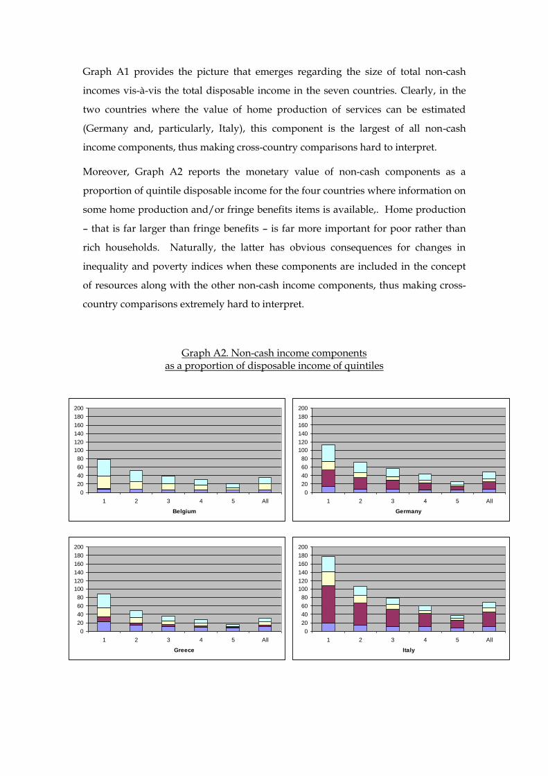
Moreover, Graph A2 reports the monetary value of non-cash components as a

proportion of quintile disposable income for the four countries where information on

some home production and/or fringe benefits items is available,. Home production

– that is far larger than fringe benefits – is far more important for poor rather than

rich households. Naturally, the latter has obvious consequences for changes in

inequality and poverty indices when these components are included in the concept

of resources along with the other non-cash income components, thus making cross-

country comparisons extremely hard to interpret.

Graph A2. Non-cash income components as a proportion of disposable income of quintiles

0

20

40

60

80

100

120

140

160

180

200

1 2 3 4 5 All

Belgium

0

20

40

60

80

100

120

140

160

180

200

1 2 3 4 5 All

Germany

0

20

40

60

80

100

120

140

160

180

200

1 2 3 4 5 All

Greece

0

20

40

60

80

100

120

140

160

180

200

1 2 3 4 5 All

Italy