Distributed Relational Database Performance in Cloud Computing: an Investigative Study Awadh Saad Althwab A thesis submitted to Auckland University of Technology In partial fulfilment of the requirements for the degree of Master of Computer and Information Sciences School of Computer and Mathematical Sciences Auckland, New Zealand 2015

Welcome message from author
This document is posted to help you gain knowledge. Please leave a comment to let me know what you think about it! Share it to your friends and learn new things together.
Transcript

Distributed Relational Database Performance
in Cloud Computing: an Investigative Study
Awadh Saad Althwab
A thesis submitted to Auckland University of Technology
In partial fulfilment of the requirements for the degree of
Master of Computer and Information Sciences
School of Computer and Mathematical Sciences
Auckland, New Zealand 2015
i
Abstract
Although the advancement of Cloud Computing (CC) has revolutionised the way in which
computational resources are employed and managed, it has also introduced performance
challenges for existing systems, such as Relational Database Management Systems
(RDBMS’). This research investigates the performance of RDBMS’ when dealing with large
amounts of distributed data in a CC environment.
This study employs a quantitative approach using positivist reductionist methodology. It
conducts nine experiments on two different RDBMS’ (SQL Server and Oracle) deployed in
CC. Also, this research does not employ any performance measurement tools that were not
specifically developed for CC. Data analysis is carried out using two different approaches: (a)
comparing the experiments’ statistics between the systems and (b) using SPSS software to
look for statistical evidence. Furthermore, this study relies on secondary data that indicate
distributed RDBMS’ generally perform better on n-tier architecture.
The results provide evidence that RDBMS’ create and apply execution plans in a manner that
does not fit CC architecture. Therefore, these systems do not fit well in a CC environment.
Also, the results from this investigation demonstrate that the known issues of distributed
RDBMS’ become worse in CC, indicating that RDBMS’ are not optimised to run on CC
architecture.
The results of this study show that the performance measures of RDBMS’ in CC are
inconsistent, which indicates that is how the public, and shared infrastructure affect
performance. This research shows that RDBMS’ in CC become network-bound in addition to
being I/O bound. Therefore, it concludes that CC creates an environment that negatively
impacts RDBMSs performance in comparison to n-tier architecture.

ii
The findings from this study indicate that the employment of the above-mentioned tools does
not present a complete picture about the performance of RDBMS’ in CC.
The results of this research imply there exists architectural issues with relational data model
thus these issues are worth studying in the future. Further, this study implies that applying
ACID creates a challenge for users who want to have a scalable relational database in a CC
environment because RDBMS should wait for the response over shared cloud network.
This thesis reports cases where serious performance issues were encountered and it
recommends that the design and architecture of RDBMS’ should be altered so that these
systems can fit CC environment.

iii
Table of Contents
Abstract ....................................................................................................................................... i Table of Contents ..................................................................................................................... iii List of Figures ........................................................................................................................... vi List of Tables ............................................................................................................................ xi Declaration ............................................................................................................................... xii Acknowledgements ................................................................................................................ xiii Copyright ................................................................................................................................ xiv
List of Abbreviations ............................................................................................................... xv
List of Acronyms .................................................................................................................... xvi .................................................................................................................................... 1
Introduction ................................................................................................................................ 1
1.0 Research problem ............................................................................................................. 1
1.1 Aim ................................................................................................................................... 1
1.2 Background ...................................................................................................................... 2
1.3 Motivations....................................................................................................................... 3
1.4 Research methodology overview ..................................................................................... 4
1.5 Research contributions ..................................................................................................... 5
1.6 Thesis structure ................................................................................................................ 6
.................................................................................................................................... 8
Literature Review....................................................................................................................... 8
2.0 Introduction ...................................................................................................................... 8
2.1 Definition of Cloud Computing ....................................................................................... 8
2.1.1 Cloud Computing features ......................................................................................... 9
2.2 Relational database management systems...................................................................... 10
2.2.1 Database................................................................................................................... 11
2.2.3 Relational data model .............................................................................................. 12
2.2.3 The role of relational database management system ............................................... 13
2.3 Problem identification .................................................................................................... 15
2.3.1 RDBMS technologies need to change ..................................................................... 17
2.3.2 A new database management system is created that takes cloud technologies into account 19
2.4 Relational database performance in CC ......................................................................... 21
2.4.1 Performance measurement tools .............................................................................. 21
2.4.2 RDBMS’ performance data in Cloud Computing ................................................... 23

iv
2.5 Conclusions .................................................................................................................... 25
.................................................................................................................................. 27
Methodology ............................................................................................................................ 27
3.0 Introduction .................................................................................................................... 27
3.1 Research method selection ............................................................................................. 28
3.2 Methodology selection ................................................................................................... 29
3.3 Methodology design ....................................................................................................... 31
3.3.1 Related studies ......................................................................................................... 31
3.3.2 Research questions and hypotheses ......................................................................... 34
3.3.3 Hypotheses testing ................................................................................................... 36
3.4 Research framework ....................................................................................................... 39
3.4.1 Investigation environment ....................................................................................... 39
3.4.2 Database architecture ............................................................................................... 41
3.5 Experiments descriptions ............................................................................................... 44
3.5.1 Experiment 1............................................................................................................ 44
3.5.2 Experiment 2............................................................................................................ 45
3.5.3 Experiment 3............................................................................................................ 46
3.5.4 Experiment 4............................................................................................................ 46
3.5.5 Experiment 5............................................................................................................ 47
3.5.6 Experiment 6............................................................................................................ 47
3.5.7 Experiment 7............................................................................................................ 48
3.5.8 Experiment 8............................................................................................................ 48
3.5.9 Experiment 9............................................................................................................ 49
3.6 Data collection................................................................................................................ 51
3.7 Data analysis .................................................................................................................. 54
3.7.1 Statistical data analysis ............................................................................................ 55
3.7.1.1 Data preparation ................................................................................................... 55
3.7.1.2 Statistical methods selection ................................................................................. 55
3.8 Theory generation .......................................................................................................... 56
3.9 Conclusions .................................................................................................................... 58
.................................................................................................................................. 59
Results Analysis and Findings ................................................................................................. 59
4.0 Introduction .................................................................................................................... 59
4.1 Pre-Experiment Preparation ........................................................................................... 60
4.2 Results and data analysis ................................................................................................ 62
4.2.1 Experiment 1............................................................................................................ 63
4.2.2 Experiment 2............................................................................................................ 71

v
4.2.3 Experiment 3............................................................................................................ 79
4.2.4 Experiment 4............................................................................................................ 88
4.2.5 Experiment 5............................................................................................................ 95
4.2.6 Experiment 6.......................................................................................................... 100
4.2.7 Experiment 7.......................................................................................................... 108
4.2.8 Experiment 8.......................................................................................................... 115
4.2.9 Experiment 9.......................................................................................................... 127
4.4 Findings ........................................................................................................................ 142
4.3.1 Performance measures in Cloud Computing ......................................................... 143
4.3.2 Performance of RDBMS’ as CDD ........................................................................ 145
4.3.3 Influence of Public Cloud Computing network ..................................................... 150
4.5 Conclusion .................................................................................................................... 153
................................................................................................................................ 156
Discussion .............................................................................................................................. 156
5.0 Introduction .................................................................................................................. 156
5.1 Performance measures in Cloud Computing ................................................................ 157
5.2 Performance of RDBMS’ as CDD ............................................................................... 159
5.3 Influence of Public Cloud Computing network ........................................................... 162
5.4 Cloud architecture VS n-tier architecture..................................................................... 164
5.5 Implications for developers .......................................................................................... 165
5.6 Conclusions .................................................................................................................. 167
................................................................................................................................ 168
Conclusion ............................................................................................................................. 168
6.1 Retrospective analysis .................................................................................................. 168
6.1.1 Performance measure in Cloud Computing ........................................................... 168
6.1.2 Performance of RDMS’ as CDD ........................................................................... 169
6.1.3 Influence of Public Cloud Computing network ..................................................... 170
6.1.4 Cloud architecture vs n-tier architecture ............................................................... 170
6.2 Further work ................................................................................................................. 170
6.3 Research limitations ..................................................................................................... 171
6.4 Conclusion .................................................................................................................... 171
References .............................................................................................................................. 173
Appendices ............................................................................................................................. 189
Appendix A ............................................................................................................................ 189
Appendix B ............................................................................................................................ 205
Appendix C ............................................................................................................................ 207
Appendix D ............................................................................................................................ 210

vi
Appendix E ............................................................................................................................ 213
List of Figures
Figure 1-1: Cloud computing ..................................................................................................... 3
Figure 3-1: Investigation environment ..................................................................................... 43
Figure 3-2: Database ERD ....................................................................................................... 43
Figure 4-1: The number of students enrolled in papers. .......................................................... 61
Figure 4-2: Snap shot of EXP1results ....................................................................................... 63
Figure 4-3: EXP1 local execution plans. ................................................................................... 63
Figure 4-4: EXP1 remote execution plans................................................................................. 64
Figure 4-5: EXP1 remote SQL Server table scan ..................................................................... 65
Figure 4-6: EXP1 duration and CPU time in seconds ............................................................... 66
Figure 4-7: EXP1 CPU time and logical reads ......................................................................... 67
Figure 4-8: EXP1 Physical reads and average I/O latency ........................................................ 67
Figure 4-9: EXP1 SQL Server wait events................................................................................ 69
Figure 4-10: EXP1 Oracle wait events ...................................................................................... 70
Figure 4-11: Snap shot of EXP2 results .................................................................................... 71
Figure 4-12: EXP2 local execution plans .................................................................................. 72
Figure 4-13: EXP2 remote execution plan ................................................................................ 74
Figure 4-14: EXP2 duration and CPU time in seconds ............................................................. 75
Figure 4-15: EXP2 Number of physical reads and average I/O latency ................................... 76
Figure 4-16: EXP2 SQL Server wait events.............................................................................. 77
Figure 4-17 :EXP2 Oracle wait events. ..................................................................................... 78
Figure 4-18: Snap shot of EXP3 results .................................................................................... 79

vii
Figure 4-19: EXP3 local execution plans .................................................................................. 80
Figure 4-20: EXP3 remote execution plans............................................................................... 82
Figure 4-21: EXP3 duration and CPU time in seconds. ............................................................ 83
Figure 4-22: EXP3 physical read and average I/O latency. ...................................................... 85
Figure 4-23: EXP3 SQL Server wait events.............................................................................. 86
Figure 4-24: EXP3 Oracle wait events. ..................................................................................... 87
Figure 4-25: Snap shot of EXP4 results .................................................................................... 88
Figure 4-26: EXP4 local execution plans .................................................................................. 89
Figure 4-27: EXP4 remote execution plans............................................................................... 90
Figure 4-28: EXP4 duration and CPU time in seconds. ............................................................ 91
Figure 4-29: EXP4 logical read and CPU time. ........................................................................ 91
Figure 4-30: EXP4 physical reads and average I/O latency. ..................................................... 92
Figure 4-31 : EXP4 SQL Server wait events............................................................................ 93
Figure 4-32: EXP4 Oracle wait events ...................................................................................... 94
Figure 4-33: Snap shot of EXP5 results .................................................................................... 95
Figure 4-34: EXP5 local execution plans. ................................................................................ 96
Figure 4-35: EXP5 remote execution plans............................................................................... 97
Figure 4-36: EXP5 duration and CPU time in seconds. ............................................................ 97
Figure 4-37: EXP5 physical reads and average I/O latency. .................................................... 98
Figure 4-38: EXP5 SQL Server wait events.............................................................................. 99
Figure 4-39: EXP5 Oracle wait events. ................................................................................... 100
Figure 4-40: Snap shot of EXP6 results .................................................................................. 101
Figure 4-41 : EXP6 local execution plans. ............................................................................. 101
Figure 4-42: EXP6 remote execution plans............................................................................. 102
Figure 4-43: EXP6 duration and CPU time. ............................................................................ 103

viii
Figure 4-44: EXP6 physical operations and average I/O latency. ........................................... 104
Figure 4-45: EXP6 SQL Server wait events............................................................................ 106
Figure 4-46: EXP6 Oracle wait events. ................................................................................... 107
Figure 4-47: Snap shot of EXP7 results ................................................................................. 109
Figure 4-48. EXP7 local Oracle execution plan. ..................................................................... 109
Figure 4-49: EXP7 remote execution plans............................................................................ 111
Figure 4-50: EXP7 duration and CPU time in seconds. .......................................................... 112
Figure 4-51: EXP7 I/O operations and average I/O latency.................................................... 113
Figure 4-52: EXP7 SQL Server wait events............................................................................ 114
Figure 4-53: EXP7 Oracle wait events. ................................................................................... 115
Figure 4-54: Snap shot of EXP8 results .................................................................................. 116
Figure 4-55: EXP8 local SQL Server execution plan. ............................................................ 116
Figure 4-56: EXP8 ORDER BY warning. .............................................................................. 117
Figure 4-57: EXP8 remote SQL Server execution plan. ........................................................ 117
Figure 4-58: EXP8 duration and CPU time in seconds. .......................................................... 118
Figure 4-59: EXP8 logical reads and CPU time. .................................................................... 119
Figure 4-60: EXP8 I/O operations and average I/O latency.................................................... 120
Figure 4-61: EXP8 tempdb I/O operations and average latency ............................................ 120
Figure 4-62: EXP8 SQL Server wait events............................................................................ 121
Figure 4-63: EXP8 Oracle wait events. ................................................................................... 122
Figure 4-64: EXP8 OSA local Oracle execution plan ............................................................ 123
Figure 4-65: EXP8 OSA remote Oracle execution plan. ........................................................ 123
Figure 4-66: EXP8 OSA duration and CPU time in seconds. ................................................. 124
Figure 4-67: EXP8 OSA I/O Operation and average I/O latency. .......................................... 124
Figure 4-68: EXP8 Oracle temp I/O operation and average I/O latency. ............................... 125

ix
Figure 4-69: EXP8 OSA wait events....................................................................................... 126
Figure 4-70: EXP9 local Oracle execution plan. .................................................................... 127
Figure 4-71: EXP9 remote Oracle execution plan. ................................................................. 128
Figure 4-72: EXP9 remote SQL Server execution plan. ........................................................ 128
Figure 4-73: EXP9 table scan .................................................................................................. 129
Figure 4-74: EXP9 segment operation .................................................................................... 129
Figure 4-75: EXP9 sequence project. ...................................................................................... 130
Figure 4-76: EXP9 clustered index insert ............................................................................... 131
Figure 4-77: EXP9 compute scalar. ........................................................................................ 131
Figure 4-78: EXP9 RID lookup operator ................................................................................ 132
Figure 4-79: EXP9 duration and CPU time in seconds. .......................................................... 133
Figure 4-80: EXP9 logical reads and CPU. ............................................................................. 134
Figure 4-81: EXP9 I/O operations and average I/O latency.................................................... 134
Figure 4-82: EXP9 TEMPDB I/O Operations and average latency. ....................................... 135
Figure 4-83: EXP9 SQL Server wait events............................................................................ 136
Figure 4-84: EXP9 Oracle wait events. ................................................................................... 137
Figure 4-85: EXP9 SSSA localSQL Server execution plan. ................................................... 138
Figure 4-86: EXP9 SSSA remote SQL Server execution plan for different approach. ........... 138
Figure 4-87: EXP9 SSSA table scan ....................................................................................... 139
Figure 4-88: EXP9 SSSA duration and CPU time in seconds. ................................................ 139
Figure 4-89: EXP9 SSSA I/O Operations and average latency. ............................................. 140
Figure 4-90: EXP9 SSSA wait events..................................................................................... 141
Figure 4-91: SQL Server duration v. CPU time. ................................................................... 146
Figure 4-92: Oracle duration v. CPU time ............................................................................. 147
Figure 4-93: Duration v. network traffic................................................................................ 152

x
Figure 4-94: Normality of simple linear regression test. ....................................................... 153

xi
List of Tables
Table 3-1: Research environment configurations .................................................................... 40
Table 3-2: Pre-experiment commands in SQL Server. ............................................................ 51
Table 3-3: Pre-experiment commands in Oracle. .................................................................... 51
Table 3-4: Skewness test .......................................................................................................... 55
Table 4-1: Average I/O latency V. number of physical reads. .............................................. 143
Table 4-2: network traffic V. runtime .................................................................................... 144
Table 4-3: T-test Descriptive ................................................................................................. 148
Table 4-4: Independent Samples Test .................................................................................... 148
Table 4-5: Correlation between Duration and Network Traffic ............................................ 151
Table 4-6: simple regression test ........................................................................................... 152

xii
Declaration
I hereby declare that this submission is my own work and that, to the best of my knowledge
and belief, it contains no material previously published or written by another person nor
material which to a substantial extent has been accepted for the qualification of any other
degree or diploma of a university or other institution of higher learning.
--------------------------------------------------
Awadh Althwab

xiii
Acknowledgements
My masters’ journey has come to an end. While I’m feeling great at this point of time, this
work has been very extensive and without the help from My God and then from some people,
it would not have been possible.
I’m thankfully to My God for giving me the strength to finish this thesis.
Dr. Alan, my primary supervisor, there are no words enough to describe my appreciation for
your help, advices and the commitments you made to my work. Thanks for ever.
I thank my secondary supervisor Shoba for your important help and the time you spent for
my masters’ work.
Special thanks to my family back home for standing by me during this journey.
Special thanks for my wife Afaf for your significant and big support and for your
understanding. Also, thanks to my son Saad.
To my mother, I lost you long time ago but you are still and you will always be in my mind.
Finally, thanks very much to my country Saudi Arabia for the very great support during my
journey.

xiv
Copyright
Copyright in text of this thesis rests with the Author. Copies (by any process) either in full, or
of extracts, may be made only in accordance with instructions given by the Author and
lodged in the library, Auckland University of Technology. Details may be obtained from the
Librarian. This page must form part of any such copies made. Further copies (by any process)
of copies made in accordance with such instructions may not be made without the permission
(in writing) of the Author. The ownership of any intellectual property rights which may be
described in this thesis is vested in the Auckland University of Technology, subject to any
prior agreement to the contrary, and may not be made available for use by third parties
without the written permission of the University, which will prescribe the terms and
conditions of any such agreement.
Further information on the conditions under which disclosures and exploitation may take
place is available from the Librarian

xv
List of Abbreviations
Exp: Experiment
ERD: Entity Relationship Diagram
R: Remote

xvi
List of Acronyms
CC: Cloud Computing
PuC: Public Cloud
WAN: Wide Area Network
RDBMS: Relational Database Management System
CDD: Cloud-Distributed Database
IS: Information System
IT: Information Technology
OLTP: Online Transaction Processing
ACID: Atomicity, Consistency, Isolation, Durability
LAN: Local Area Network
DBMS: Database Management Systems
EC2: Amazon Elastic Cloud Computing
SSSA: SQL Server Second Approach
OSA: Oracle Second Approach
AWR: Automatic Workload Repository

Chapter 1 Introduction
1
Introduction
1.0 Research problem
CC environment creates new challenges that can negatively impact the performance of the
deployed technologies. Using virtualization, the underlying hardware such as, CPU and
Memory is shared among multiple users. Therefore, it is important that the performance of
RDBMS is investigated when deployed in a CC platform. This research asks questions which
are detailed in Section 3.3.2, p. 35-36. These questions look to examine the effect of CC on
relational databases in terms of the performance and the query optimisation.
1.1 Aim
Any distributed RDBMS requires a network and nodes. The characteristics of CC
architecture is different from architectures such as n-tier architecture. The differences appear
in that the CC architecture depends on the Internet and relies on virtualisation that abstract
the physical architecture (Ivanov, 2013, Khajeh-Hosseini, Greenwood & Sommerville, 2010).
Also, an n-tier architecture operates on a client/server model and includes a database system
that stores data, while the server application and users access the database system using the
middleware in the n-tier architecture (Frerking et al, 2004; Eriksson, 2015). In CC, the user
may obtain more direct access to data or may access data via a Services Oriented
Architecture (SOA). In n-tier architecture, these nodes exist within a data centre’s networks
between servers and racks but these have significant bandwidth (Benson, Akella & Maltz,
2010) compared to the cloud architecture where limited and shared bandwidth exists, for both

Chapter 1 Introduction
2
internal and external networks (Moens & Turck, 2015). However, distributed RDBMS’ in n-
tier architecture suffer from performance issues related to query optimisation (Chaudhuri,
2012b; Liu & Yu, 1993; Mullins, 1996 & Tewari, 2013). Therefore, since RDBMS’ normally
operate on n-tier architecture (Frerking et al., 2004), the present thesis aims to investigate
RDBMS’ performance operating on a cloud architecture.
1.2 Background
CC appears to have gained more attention in recent years. This is especially important since
the world is increasingly a witness of enormous growth in data volume. For instance, it is
extrapolated that such volume will reach the peak of 7.2 zetabytes by 2015, which is
equivalent to 7.2 trillion gigabytes (Litchfield & Althouse, 2014). Indeed, such a figure
illustrates the fact that there is a continuous need for advancing Database Management
Systems (DBMS) to handle that growth especially when the data that being created are
largely stored in databases. CC can play a central role in hosting these databases because
multiple features are provided by CC including, but not limited to, the ability to control
spending on Information Technology (IT) services (Armbrust et al., 2010).
CC relies heavily on virtual machines (Zhan, Liu, Zhang, Li & Chung, 2015). Virtual
machines (VM) involve computer systems that emulate the processes of real computer
infrastructures. There are many commercial VM products that can support virtualisation, such
as EXC/ESXI server, Microsoft Hyper-V R2 and Proxmox Virtual Environment (Litchfield
& Althouse, 2014). This way virtualisation supports the allocation and delivery of
computation to CC users.

Chapter 1 Introduction
3
Figure 1-1: Cloud computing
This figure is obtained from (Wiggins, 2009)
CC can be thought of as a distributed system because users can access to VMs via Wide Area
Network (WAN). While such characteristics may help for achieving reduction in spending
on IT services, the network between the nodes mostly is the WAN and the loads are
unpredictable and variable (Litchfield & Althouse, 2014). Further, CC offers a method of
accessing to a shared pool of computing resources such as network, disks, servers and storage
(Ferris, 2015; Marcon et al., 2015).
This research considers CC as system with virtual memory and CPU. Moreover, CC
enable users to have more than one node so that users can distribute their system and data
across multiple nodes. CC provides a platform that this research employs to investigate the
performance of RDBMS’ in such environment. Thus this study introduces the term Cloud-
Distributed Database (CDD).
1.3 Motivations
CC provides a platform which can be used for accommodating ever-growing data volume
using any particular DBMS. CC service provider manages configuration and privacy of the
underlying infrastructure while the DBMS is being responsible for database optimisation.
Further, Litchfield and Althouse (2014) carry out a systematic review that implies CC
increasingly becomes a mainstream technology in dealing with large datasets. Moreover,

Chapter 1 Introduction
4
McKendrick’s (2012) shows that 13% of large organisations (>10000 employees) were
currently hosting their DBMS’ on cloud-based server and 18% of them would deploy their
DBMS in CC environment by 2013.
Secondly, RDBMS’ were established on the relational data model (Codd, 1970) and
have now existed for more than four decades. The model has gained wild popularity in the
industry and it is the standard model for business databases (Suciu, 2001). More recently,
McKendrick’s (2012) study indicates that 77% of study’s sample consider structured data as
central to their daily business activities. More importantly, RDBMS’ are still mainstream
technology as means for data management (McKendrick, 2012). The study also shows that
92% of its sample use RDBMS’ compared to 11% who employ NOSQL databases (see
Appendix E, pp. 212 – 213, for extended discussions about NOSQL systems).
In order to identify the extent to which RDBMS’ are affected by influences from
cloud architecture and may result in inadequate performance, this research therefore
undertakes an experimental investigation into RDBMS’ performance in CDD.
1.4 Research methodology overview
Since this research attempts to examine and identify RDBMS’ performance in CDD, it needs
empirical data in order to achieve its purposes. The selection process of methodology
considers many methods and the selection arrives at adapting positivist reductionist approach.
Further, a large dataset is used to help with quantifying RDBMS’ performance in
CDD by executing a variety of experiments on two RDBMS’ namely SQL Server and Oracle.
The experimental scenarios represent real-world uses of RDBMS. However, some real-world
queries, such as arithmetic queries, could not be performed in this study because the dataset
that is used does not contain appropriate data. Of all the queries, some are relatively easy to
process with no large datasets returned, but the majority are either long processing queries

Chapter 1 Introduction
5
with a degree of complexity or the returned result is large. In all experiments, in order to
perform the query the joining of at least two tables is required. However, query conditions
that need to be satisfied are based on the parent or child tables or both of them. The systems
reside on virtual servers located in Auckland, New Zealand and Amsterdam, the Netherlands.
Each system has two VMs, one of which is located in Auckland (remote) and stores MYTABLE
and the other VM is located in Amsterdam (local) and contains the parent tables.
This research assumes the following:
1. That the RDBMS’ are optimised for use in an n-tier architecture.
2. That queries are optimised on the RDBMS to provide high performance output when
data sets are readily available on the server.
3. That large data sets would not normally be widely distributed.
4. Large datasets would normally be replicated rather than distributed.
1.5 Research contributions
The contributions of this research are as follows:
1. This study adds to Information System (IS) literature by demonstrating that current
RDBMS’ do not fit CC environment. RDBMS’ suffer from performance issues in n-
tier architecture and in cloud architecture. That is, they do not efficiently process large
datasets distributed over cloud or public network.
2. This research also verifies that RDBMS’ are optimised to be deployed over n-tier
architecture so that any issues with distributed RDBMS’ are intensified in a Cloud-
based environment.

Chapter 1 Introduction
6
3. This research provides a methodical approach to examining the performance of
RDBMS’ in a CC environment where multiple variables can affect their performance.
Such approach contributes to IS literature by showing that measuring RDBMS
performance in CC using tools that are not originally developed for use in CC does
not give a complete picture.
4. This study contributes to IS literature by showing that RDBMS’ in cloud architecture
are not only I/O bound, but also become network-bound.
1.6 Thesis structure
The thesis consists of six chapters. Chapter 1 (the current chapter) introduces the research by
giving the background of the topic and explaining the motivation behind the research. This
chapter also gives an overview of the methodology employed and concludes by outlining the
study’s contributions and the thesis’s structure.
Chapter 2 provides a review of current and past literature and a critique of the relevant
body of knowledge concerning both CC and RDBMSs. The chapter summarises the main
points of the topic so that research direction is clearly identified. One point indicates that
there is no adequate performance investigation that is related to RDBMS’ deployed in cloud-
based environment and there is a need to identify RDBMS’ performance issues this
environment. The other point indicates that most of RDBMS’ related performance data are
obtained using performance measurement tools that are not originally developed to run in the
Cloud. Therefore, this research avoids these tools and forms its performance measurement
approach which Chapter 3 describes. The conclusion of Chapter 2 specifies the research
questions and establishes its hypotheses.
Chapter 3 discusses the process whereby the methodology is selected. The research
framework is explained by describing the investigation environment where the experiments

Chapter 1 Introduction
7
are conducted and demonstrating the database architecture that is used. Chapter 3 also details
each experiment conducted in this research. The chapter moves on to outline the data
collection steps and how data analysis is conducted. Before the chapter concludes, the
process of theory generation is explained.
Chapter 4 presents the analysis of the experiments described in Chapter 3. Each
experiment is compared between SQL Server and Oracle. The comparisons use the
performance measures identified in Section 3.3.2. Chapter 4 also presents the findings of this
research. The findings section contains statistical analysis to explain these findings in
statistical manner. Moreover, the chapter shows whether or not the stated hypotheses can be
accepted or rejected
Chapter 5 evaluates the findings outlined in Chapter 4. Chapter 5 addresses the
research questions and provides answer to them. The chapter compares and contrasts the
findings with the existing body of knowledge described in the Literature Review chapter.
Chapter 6 concludes the thesis by summarising the findings of the research and also
by describing the study’s limitations. The chapter concludes by proposing some further
research direction.

Chapter 2 Literature Review
8
Literature Review
2.0 Introduction
The goal of this chapter is to critically analyse the existing body of knowledge with regards to
relational database performance issues in CDD. By identifying such issues, the chapter paves
the way to experimentally determine potential impact of CC environment on performance.
Chapter 2 is organised into five sections that provide extended summaries of relevant
key issues and specify potential directions for the research. Section 2.1 defines cloud
computing and describes its relevant features. Section 2.2 defines RDBMS’ and relational
data model and provides a comparison between this model and preceding data models. This
section also explains the role of RDBMS’. Section 2.3 identifies the research’s direction and
illustrates that the literature creates different positions towards data management in CDD.
Section 2.4 offers an overview of works that are similar to this research. Finally, Chapter 2
concludes by providing potential research questions and establishing hypotheses.
2.1 Definition of Cloud Computing
Since this research is conducted to examine relational database performance CC, this section,
explains CC in details and its implications to relational database and large datasets.
Various definitions of CC are observed in the literature that encompass the elements
of CC in a more specific manner, although they differ considerably in which aspect of CC
they cover. For instance, definitions by Geelan (2009) and Buyya, Yeo and Venugopal (2008)
define CC based on economies of scale, especially when allowing users to choose the amount
of resources they can use and therefore reduce the overall cost of utilising cloud

Chapter 2 Literature Review
9
infrastructures. Moreover, they focus on providing service level agreements (SLA) between
service providers and consumers while maintaining a certain level of quality of services.
These definitions also imply that CC features, including scalability and the ability to optimise
the use of resources, play a key role in empowering users to have full control over their
spending on IT services (Vaquero, Rodero-Merino, Caceres & Lindner, 2008).
CC can be defined as: “a large pool of easily usable and accessible virtualised
resources. These resources can be dynamically reconfigured to adjust to a variable load
(scale), allowing also for an optimum resource utilization” (Vaquero, Rodero-Merino,
Caceres & Lindner, 2008, p.52). These resources are typically consumed by a pay-per-use
model and services providers are responsible for guaranteeing the needed infrastructure at an
agreed SLA (Geelan, 2009).
2.1.1 Cloud Computing features
Cloud computing has three models of service, namely public clouds, private clouds, and
hybrid clouds (Geelan, 2009). These models differ in terms of the management of the cloud.
Public Cloud (PuC) involves many customers accessing the cloud from different locations
using the same infrastructure (such as via the Internet). The private cloud in which the
management can either be undertaken by the organisation itself or outsourced. The
implications for an organisation with a private cloud are significant, and this is especially
important because access to its resources is more limited than a PuC. A hybrid cloud on the
other hand, involves combining public and private clouds to facilitate the expansion of the
private cloud using the resources of the public cloud.
One important feature the Cloud-based environment has to offer is a high level of
service availability (Litchfield & Althouse, 2014). This includes data availability and other IT
resources. On the other hand, moving to a cloud platform does not guarantee data to be

Chapter 2 Literature Review
10
always accessible and performance bottlenecks can potentially lead to data unavailability, be
it technical bottlenecks or network insufficiency (Litchfield & Althouse, 2014). Database
locking, lack of storage capacity (such as in Thakar, Szalay, Church and Terzis (2011)) and
cache flushing, for example, can also cause bottlenecks in cloud systems. Network
insufficiency in PuCs is an important cause for performance bottlenecks and data
unavailability especially when data move between cloud nodes within limited bandwidths
(Litchfield & Althouse, 2014).
This research conducts its experiments on PuCs and the effects of PuC use on
performance are important to consider. Li, Yang, Kandula and Zhang (2010) conduct a
comparison between PuCs and conclude that there are considerable differences between PuC
providers and this imposes challenges as to which PuC provider to go with. Further, although
Iosup et al., (2011) PuCs appear to suit small databases and show deficiencies when
employed for heavy workloads coming from the scientific field, Thakar et al. (2011) and
Hashem (2015) disagree with such claim and indicate that PuC such as Amazon Elastic
Cloud Computing (EC2) and Microsoft SQL Azure can be used for scientific tasks.
Gunarathne Wu, Qiu and Fox (2010) add that PuCs can be used in cases (such as big data
tasks) where there are complex queries request intensive computation resources that need to
be performed on high dimensional data residing on heterogeneous databases. But since PuCs
operate on shared infrastructure using VM, such configurations cause I/O performance to be
inconsistent.
2.2 Relational database management systems
The previous section defines and discusses CC. This section explains and discusses RDBMS’
that this research investigates their performance in CDD.

Chapter 2 Literature Review
11
2.2.1 Database
Database in itself implies a collection of data grouped together for at least storage purposes
(Connolly & Begg, 2005). What is stored inside have no meaning until they are put into some
context that is related to purpose of the database. This suggests that a database needs to have
a collection of related data managed by a system such as DBMS. However, this definition
seems general, and hence any related data stored in any random file can be called a database
while in the real-world situation a database reflects some restrictions, and they include the
following points (Connolly & Begg, 2005):
• A database represents a collection of data inherently holding some meaning and put
together in a logical and coherent manner. Therefore, an assortment of random data
does not directly constitute a database.
• A database represents an aspect of a real-world situation, that when changes occur to
this situation the database will reflect these changes, and this implies consistency.
• Database design serves a specific purpose and hence has related data intended to
respond to requests from a known group of users and applications to be used by these
users.
That said, a real-world database has users who are interested in accessing the contents of a
database, and interactions occur between users and the database; in other words, they are
interacting with the real-world situation itself (Connolly & Begg, 2005). Such contents are
usually generated or derived from data sources related to this situation. Thus a database can
be defined as “a shared collection of logically related data, and a description of this data,
designed to meet the information needs of an organisation” (Connolly & Begg, 2005, p. 15).

Chapter 2 Literature Review
12
2.2.3 Relational data model
The relational data model which RDBMS’ are built upon uses operators, namely permutation,
projection and join to derive relationships from other relations. A relation is table where it has
tuples that have attributes and has columns and rows. A relationship exists between two or
relations.
Hawthorn and Stonebraker (1979) examine the performance of the INGRES relational
database from overhead-intensive, data-intensive and multi-relation queries. Overhead-
intensive represents queries with little data to be returned. In this regard, performing such a
query depends on the nature of applications, whether there is a locality of reference or not.
Data-intensive queries represent the time taken to process by the database. It concludes that
buffer size is an important factor for processing queries, and this becomes an issue when the
size of the relation is larger. Bell (1988) agrees with this conclusion and adds that the buffer
manager of the database can lead to overall performance degradation, especially when there
is a divergence between the buffer manager and how the operating system handles the page
placement on the disk. Only by having a larger memory can performance improve; otherwise
it will be subject to a transaction execution requirement such as the size of the relation and
whether there is an update query (Blakely & Martin, 1990). Furthermore, Michels, Mittman
and Carlson (1976) compare the relational and network databases, and acknowledge that the
network database allows more efficient handling of queries because the programmer can
direct the system to the target piece of information, reducing the need to develop algorithms
to determine an efficient execution plan. Additionally, Stonebraker and Held (1970)
demonstrate that despite the complexity in coding optimised queries in hierarchical and
network databases (see Appendix B, pp. 204-205 for description), they have a better
performance compared with the relational database where the user does not have control over
the query optimisation process. Stonebraker et al. (1990) conclude that the complexity of

Chapter 2 Literature Review
13
coding optimised queries has in fact resulted in performance issues. However, while Michels
et al. (1976) agree that the availability of query optimisation techniques has a large influence
on improving the performance of the relational database, implying the benefit from its
mathematical foundation. Another study illustrates that a relational database cannot provide a
solution to every real-world situation and gives practical evidence that a relational database
does not necessarily suit a hierarchical structure of clinical trials data (Helms & McCanless,
1990).
In summary, databases including relational, network and hierarchical put considerable
attention on optimisation. In, network and hierarchical databases, the programmers can
intervene in choosing desirable execution plans but they lead to performance issues.
Relational databases have multiple optimisation methods that RDBMS’ control and they can
improve the performance. These databases are developed before cloud architecture comes
into existence.
2.2.3 The role of relational database management system
RDBMS’ are involved in almost every aspect of life that requires storing or manipulating of
data where the data are to be used to conduct trade, medicine, education and so forth.
RDBMS’ operationalise relational model in which collection of tables is used to store data.
Mostly, each table has a primary key of a group or group of fields that identifies each tuple in
a table, implying that each table is unique and has only one primary key. RDBMS allows the
user to declare the rules by which the relations are to be established where there is a common
attribute (Connolly & Begg, 2005). Further, RDBMS’ put a large emphasis on data integrity
and hence employ multiple concepts such as Atomicity, Consistency, Isolation and Durability
(ACID) properties (Connolly & Begg, 2005). ACID properties include Atomicity, which
means all of a transaction’s operations are successfully done otherwise the transaction will be
rejected. Consistency means that the database moves to a new consistent state on execution of

Chapter 2 Literature Review
14
each transaction. Isolation makes sure no interference occurs between transactions. Durability
ensures that in case of database failure, committed transactions will not be undone (Connolly
& Begg, 2005).
Query optimisation is another important task that RDBMS’ have to perform. Thus
there have been a significant body of knowledge related to providing highly efficient methods
for query optimisation. The choice of an efficient plan appears to be a complex task, since
there are many variables that are computed. For instance, the RDBMS have to estimate
number of tuples that query selects and the number of tuples retrieved by every operation that
the execution plan performs. The RDBMS also needs to estimate the computational resource
required for the execution so that it uses CPU usage, I/O and memory as variable for the
estimation. Moreover, RDBMS may compare plans before it chooses one plan (Chaudhuri,
Dayal, Narasayya, 2011).
Query optimisation approaches enable RDBMS to have many ways by which query
executions can be efficiently carried out (Connolly & Begg, 2005). However, Shao, Liu, Li
and Liu (2015) believe that there appears to be issues with the existing optimisation methods
performance and, the authors present a new optimisation system for SQL Server that is based
on a hierarchical queuing network model. With this model they achieve on average a 16.8%
improvement in the performance of SQL Server compared with existing optimisation
methods, and increases transaction throughput by 40%.
Further, query optimisation in a distributed environment poses challenges that appear
persistent (Chaudhuri, 2012b). Distributed environment adds complexity for query
optimisations since it involves the possibility to move data between location(s) in order “for
intermediate operations in optimizing a query” (Chaudhuri, 1998a, p. 41) and by doing so, the
distributed system adds more variables into the equation of computing best execution plans

Chapter 2 Literature Review
15
(Mullins, 1996; M. Khan, & M. N. A. Khan, 2013). Liu & Yu (1993) recommend that more
investigation is needed in order to determine whether or not the inefficient implementation or
unsuitable execution plans chosen by the RDBMS’ cause long-processing queries. Their
work is about evaluating three algorithms using many parameters such as the number of
processing locations and the amount of data that are to be joined. It concludes, among other
factors, network overhead is observed to be a major influencer, although the study is
conducted on Local Area Network (LAN). More recently though, the issue remains unsolved
and there is a need to revisit the traditional optimisation methods since NOSQL databases
introduce new approaches for query optimisation that appear to be providing a better
performance when these methods are employed for large dataset processing in a distributed
database (Zhang, Yu, Zhang,Wang & Li, 2012; Chaudhuri, 2012b).
2.3 Problem identification
Bell, Hey, & Szalay, (2009) state that “data-intensive science has been slow to develop due to
the subtleties of databases, schemas, and ontologies, and a general lack of understanding of
these topics by the scientific community” p.1298. CC poses challenges related to the
deployments of database systems such as relational databases, which, with the emergence of
CC, have become obstacles in using database management systems in CC (Zhang, Yu,
Zhang, Wang & Li, 2012). That is, the scholarship does not in fact provide a single
exemplary design for a database management system that can fit CC environment (Agrawal,
Das, & El Abbadi, as cited in Litchfield & Althouse, 2014).
Codd (1970) sees an opportunity that instead of storing data in a data bank, they can
be organised into tables and then related based on common data. This also helps to remove
redundancies and keep data in a consistent state. The practice of RDBMS has been on a
client-server model where systems communicate with the computer hardware (see Section

Chapter 2 Literature Review
16
1.0). Revolutionary changes that have occurred in data volume and infrastructure and
platform technology development (cloud computing) lead to revealing that such RDBMS
appear to cope less well with these changes (Zhang, Yu, Zhang,Wang & Li, 2012). The
pattern observed in the literature signals that there are conflicting views as to whether
RDBMS’ can still be used in the era of large datasets. These views indicate that architectural
issues exist with the relational data model that prevent it from being effective in combating
large datasets in CC and these issues erode relational databases’ benefit (Litchfield &
Althouse, 2014). The other view however, states that RDBMS’ are still important for many
stakeholders (banking systems and airline companies) and in order for satisfactory
performance, modifications need to be made to relational databases before deploying them on
cloud systems (Cattell, 2011; Arora & Gupta, 2012). Such changes involve taking into
account ACID properties.
Further, Zheng et al. (2014) demonstrate how the relational data model can be
extended to perform “big data” business tasks. It is proposed that with inspiration of NOSQL
data models such Key-value models (see Appendix E, p. 212-213), relational data model can
overcome performance issues when large datasets are under processing. Durham, Rosen and
Harrison (2014) indicate that large datasets pose challenges in handling them and the data
model can be a significant limiting factor in such handling. Therefore they make the claim
that RDBMS’ do not perform efficiently with “big data”. When dealing with ‘big data’,
pulling the data across the network impacts performance, implying that joins of distributed
tables should be avoided. Instead the database engine, which they believe it is capable of
handling of large datasets, can be leveraged by the use of stored procedures inside the
database (Durham, Rosen & Harrison, 2014).
Therefore, this investigation aims to identify potential performance issues and
proposes methodical assessments in regards to RDBMS’ in CDD. To achieve these goals, the

Chapter 2 Literature Review
17
investigation undertakes an experimental work on a non-optimised system and it employs
approaches including distribution of the RDBMS’ across the WAN so that distributed queries
are undertaken using a large dataset.
This research presents the argument that cloud technologies have introduced many
technical issues that affect relational database performance and these can be attributed to one
of the following propositions.
1. RDBMS technologies need to change
2. A new database management system is created that takes cloud technologies into
account.
In addition to these propositions, this research reveals that there appears inadequate data
concerned with RDBMS’ performance in CDD when a large dataset is being dealt with;
therefore this research identifies the issue and proposes the need for RDBMS performance
data in CDD, using existing measures for comparison.
2.3.1 RDBMS technologies need to change
It is believed that RDBMS’ demonstrate less capability to meet the performance required for
handling ever-growing data in CC, and this issue becomes clearer as the amount of data
increases (Liu, X, Shroff, & Zhang, 2013). However, according to Hacigumus et al. (2010)
RDBMS performance needs further investigation to determine whether or not RDBMS’ are
sufficient to meet the challenge of large datasets. Moreover, RDBMS should not be blamed
for such performance issues; rather it is the operating technology that needs improving so
RDBMS can provide the expected performance (Feuerlicht & Pokorný, 2013). However,
although the denormalisation of relational databases appears to have introduced data
redundancy, it reduces the number of table joins and therefore easing table joining effects on
performance (Sanders & Shin, 2001).

Chapter 2 Literature Review
18
Further, this literature review notices that there is an increasing pattern towards
identifying if there is a role that RDBMS’ play behind performance struggles. For instance,
there is an extensive scholarship concerning query optimisations due to the central role that
they play in performance improvement (Liu & Yu, 1993) and therefore multiples and
different algorithms are developed including but not limited to greedy and approximation
algorithms. However, when it comes to heavy workload, query optimisation methods show
deficiencies (Kalnis & Papadias, 2003). Add to that Batra and Tyagi (2012) think RDBMS’
are no longer applying join as efficiently as required, and the study argues that as the dataset
size grows, the search for matching tuples takes a longer time and, therefore, the join
becomes a performance bottleneck. From these points, it can be concluded that query
optimisation methods in RDBMS’ suffer from shortcomings, although they are deployed over
architecture that is different from cloud architecture.
As previously mentioned, CC poses challenges for the deployment of RDBMS’. Chen
et al. (2010) claim that while the relational data model is widely used, the model negatively
impacts performance in cloud deployment and is replaced by key-value data models that they
recently start to take the attention in data management. Leavitt (2010) adds that even if
powerful hardware is in place to for achieving high performance, the practicality of RDBMS
nearly always involves distributing the database to multiple users that are geographically
distributed, and this is where the struggle in performance emerges due to the type of queries
in which joining of distributed tables is usually necessary. When RDBMS’ deployed over
cloud architecture, the systems need optimisation techniques that fit such architecture and
facture by the ability to detect and adjust to workload fluctuations Mathur, Mathur &
Upadhyay, 2011).
In CC architecture, the lack of suitable optimisation methods can lead to suboptimal
choices made by these approaches and these choices are especially important over large

Chapter 2 Literature Review
19
datasets (Ganapathi, Chen, Fox, Katz & Patterson, 2010). As an example, while subqueries
are common in relational database, they can lead to performance issues if they are not
performed as efficient as required. Certainly, they create performance issues in data
warehouse applications (Kerkad Bellatreche, Richard, Ordonez & Geniet, 2014). Dokeroglu,
Bayir and Cosar (2015) indicate that such overheads can be reduced if subqueries are
executed only once, and propose a set of algorithms to enable cloud relational databases to
make better choices when creating an execution plan. A possible choice is to decide where to
perform the join so that the effect of the network on performance is reduced.
Therefore, current RDBMS’ appear to have significant shortcomings in performing its
key theme in large dataset management in CC, and they need to change.
2.3.2 A new database management system is created that takes cloud
technologies into account
The discussions above present that RDBMS’ appear to have issues that preclude the ordinary
deployment in cloud technologies, thereby necessitating the development of solutions to work
around such issues. However, this section aims to discuss what the literature offers in regards
to providing RDBMS’ that fit cloud technologies.
CC can be considered as a distributed environment that allows users to have their
database distributed and be connected via the Internet, and also the promise that enables users
to add more computational resources when needed (see Section 1.0). There are many designs
that aim to provide an architecture that fits CC; mostly these designs focus on data
partitioning. For instance, inspired by the concept that web-based workloads are mostly
limited to single object access, Das, Agrawal and Abbadi (2009) describe a transactional
database for the CC that complies with ACID properties. These properties apply in this

Chapter 2 Literature Review
20
system in each partition so the system avoids applying them across partitions. In other words,
full consistency can be guaranteed when the sum of all consistent parts are added together.
Curino et al. (2011) propose a relational database for CC in which they aim to reduce
any unnecessary scanning of multiple nodes. Aimed at no more than one node should involve
the execution of queries. They want to avoid I/O overhead and reduce unneeded
communication overhead. The approach partitions the database based on a graph data
algorithm. Such approach works by analysing the complexity of workloads and mapping the
data item to appropriate nodes.
The LogBase (Vo et al., 2012) system aims to exploit the log-only storage approach to
eliminate the write bottleneck. It deploys the log as core data storage in which updates are
appended at the end of the log file; thus there is no need for the updates to be reflected into
other files (such as in any database). The developers of the system use vertical partitioning to
improve I/O performance. That is, the columns of tables are clustered into a group of
columns that are stored separately in varying physical data partition locations in accordance
with the frequency of access requested by the workloads. This helps the LogBase benefit
from the locality of data when executing queries and to avoid the overhead of distributed
transactions. Further, the system applies ACID properties on a single row of data, similar to
some NOSQL systems such as Pnuts (Cooper et al., 2008), Cassandra (Lakshman & Malik,
2010) and HBase (http://hbase.apache.org).
This section presents what the literature has to offer in regard to creating database
management systems that suit cloud technologies. The discussed systems focus in reducing
cloud network overhead be it, when data move between nodes or the I/O overhead.
Moreover, ACID properties can still be conformed but only within data partitions. Therefore,

Chapter 2 Literature Review
21
though there are inconsistencies in their approaches to ACID guarantee, it appears that a new
RDBMS is created that can fit cloud technologies.
2.4 Relational database performance in CC
The above discussions show that RDBMS’ need changes so they can cope with ever-
increasing data volume in CC. This section aims to explore performance-related data that are
concerned with what measuring tools are actually in use and to explain as to whether such
tools are appropriate to CC. The literature offers previous studies in regards to relational
databases in CC and this section therefore outlines them.
2.4.1 Performance measurement tools
The deployment of DBMS over cloud network appears to have introduced challenges towards
measuring the performance of such deployment. The measurements of DBMS performance in
general have been undertaken by benchmarking tools and, as an example, Transaction
Processing Performance Council tools (TPC) (TPC, n.d,). That is, some tools, such as
SPECCpu benchmark, work to evaluate any given computer system and recommend the best
CPU for the workload (Folkerts et al., 2013), while TPC-C evaluates DBMS that suit Online
Transaction Processing (OLTP) applications (Kiefer et al., 2012). Other tools serve different
purposes. For instance, in 1980, a benchmark tool named Wisconsin benchmark is developed
to evaluate and compare different relational database systems (DeWitt, 1993). It consists of
32 queries to test the performance of relational view operations, with the inclusion of
selection, aggregation, deletion and insertion queries. Following this, a tool called the debit-
credit benchmark is specifically developed for evaluating the transaction processing
capabilities of DBMS. This involves applications such as a banking application where
multiple users simultaneously access the database (Carey, 2013). Further, TPC methods cater
for measuring the performance of DBMS as a result of the advances in its underlying

Chapter 2 Literature Review
22
hardware and software. For instance, TPC-C caters for more complex applications such as
inventory management applications (Nambiar, et al., 2012). Other benchmarks are
established specifically to benchmark database systems – for example, OO7 for an object-
oriented database, Sequoia for a scientific database, and XMark for an XML database (Carey,
2013).
This research observes that there is an extensive utilisation of TPC-C to measure the
performance of the database in CC there is little attention is put in place for considering the
characteristics of CC when undertaking the measurement of RDBMS performance. These
tools are used to carry out performance evaluation for commercial cloud services (such as in
Kohler & Specht, 2014). The implications may be significant for the accuracy of these
experiments since the examination tools are developed to cater for the static environment,
which raises concerns as to their appropriateness for CC environment. Curino et al. (2011),
report on (among other features) the performance of relational cloud database scalability.
Interestingly, in Curino et al. (2011) experiment, the TPC-C instances exhibit poor
performance compared with when a relational cloud system is in place. The relational cloud
system scales fine and achieves higher throughput and experiences low latency compared to
TPC-C instances. Therefore, not only is more performance data needed for a greater level of
certainty around the performance of RDBMS in CC, but also it matters which method is used
to measure performance.
This research observes a growing interest in tackling experiments for DBMS
performance in CC using a suitable tool. Study carries out by Binnig, Kossmann, Kraska and
Loesing (2009) indicates that as TPC benchmark tools are originally developed for the static
environment tools they are not adequate for CC. Although they are still relevant to the cloud,
they lack the ability to measure the dynamic systems deployed in the cloud, and also the
feature of CC. In this regard, Yahoo! develops its own benchmarking tool for measuring

Chapter 2 Literature Review
23
cloud database performance. They claim that existing tools such as TPC-C may not match
CC characteristics. Smith (2013) argues, however, that there is a need for a cloud
benchmarking tool and proposes a method that leverages the existing TPC-C and TPC-E to
produce a TPC-VMC. The core design of this method is that the characterisation of database
performance should be based on a limited cloud environment in terms of the number of
servers, hardware footprints or system costs. This determines that the performance of DBMS
in the cloud can be measured using TPC tools but with the limitation of the cloud
environment.
2.4.2 RDBMS’ performance data in Cloud Computing
Further, there appears a pattern in the literature that inadequately demonstrates RDBMS’
performance in CDD. They also focus mainly on testing whether virtualisation technologies
such as VMware have an impact on database performance. For instance, Minhas, Yadav,
Aboulnaga and Salem (2008) examine the performance of a relational database in a
virtualised environment using TPC-H workload. The authors conclude that running a
database over virtualised environment creates I/O disk overhead but that such an overhead
does not have a large impact during the runtime of queries. The study indicates that this
overhead is an average of %10 or less of the runtime. Furthermore, Bose, Mishra,
Sethuraman &Taheri (2009) study the effect of virtualisation technology namely ESX Server
4.0 on Oracle Database 11g R1 and Microsoft SQL Server 2008. The study employs TPC
workloads to make a comparison between the performance of these database system in and
off cloud. It finds out that although these RDBMS’ perform better off cloud, they achieve
between 85% and 92% of native performance in CC and therefore it concludes that CC is
“capable of handling database-intensive workloads” p. 181. However, while Ivanov, Petrov
& Buchmann (2012) conclude that CC is more suitable for read-mostly work and for other

Chapter 2 Literature Review
24
purposes such OLTP applications and data-intensive workloads CC poses challenges;
however they work around such challenges by adding more buffer.
Recent study aims to examine how RDBMS’ perform in CDD. For instance, Kohler
and Specht (2014) conduct comparisons between two RDBMS’ in which both systems have
different configurations. Their approach is to partition a single table across multiple cloud
providers including private and PuC. Performance is generally better when the experiments
are conducted off cloud. For instance, when the experiment returns one tuple, it takes 265 ms
but with network latency the duration reaches as high as 319 ms. Since their data are
partitioned they also notice a high join overhead. However, the present study is different in
1) it does not employ any benchmark tools, 2) it uses large datasets and creates its own
experiments, 3) the used RDBMS’ are installed on identical configurations so that the
investigation becomes comparative.
Further, Thakar et al. (2011) perform analytics work on large databases using two CC
platforms, namely EC2 and Microsoft SQL Azure, and then they compare performance data
with their non-cloud system. Their database stores several TB. However, it is not possible to
migrate the whole database due to limitation on the size these platforms can host. Eventually,
they transfer 100 GB via the cloud to EC2 in this instance and only 10GB to Azure since it is
the maximum limit that an instance can store. Yet the paper reports only a comparison of
experiments conducted on 100 GB in and out of the cloud. Overall, experiments run faster on
n-tier architecture due to a “number of factors, such as the database settings on the EC2
server (memory, recovery model, tempdb size, etc.) as well as the disk speeds”; they also
indicate that “the performance in the cloud can be disappointing unless it can be tuned
properly” (Thakar et al., 2011, p.150) .

Chapter 2 Literature Review
25
2.5 Conclusions
CC platforms are of significance to the database research field and to businesses, as they
provide scalability, elasticity and availability of IT resources. However, they create
RDBMS’ appear to display performance issues and therefore other database systems such as
NOSQL gradually start to grasp the attention in data management. NOSQL avoids complex
queries that involve joining of distributed tables, while in relational databases, such practice
is commonplace. Whether RDBMS’ perform such joining operations a manner efficient that
takes into account the amount of the data is another question.
Multiple “work-around” have emerged to improve RDBMS’ capability to be deployed
in CC. The literature also shows inadequate demonstrations of RDBMS’ performance in CC.
For example, there are performance issues with query optimisation in distributed RDBMS’
deployed in an n-tier architecture. Therefore, this research conducts an experimental
investigation aimed at identifying potential break points that RDBMS’ have when processing
large datasets in CC architecture. The results can be used to develop a database management
system that suits CC or improves the existing RDBMS solutions for clouds.
Performance data for RDBMS in clouds appears to be derived from mostly unsuitable
tools. This research disagree with the use of such tools in CC environment. Therefore, this
research aims to carry out a performance investigation for RDBMS in CDD by using other
methods.
Therefore, this research asks the following questions accompanied with working
hypothetical statements:
RQ1: What are performance measures that can be applied to examine RDBMS’
performance in CC?

Chapter 2 Literature Review
26
RQ2: Are the measures related to Q1 valid for measuring RDBMSs in the clouds
when large datasets are being manipulated?
H1: There is no consistent measure of performance when comparing RDBMSs
operating in CC.
RQ3: What evidence exists that RDBMS’ are creating significant performance issues
in a cloud-computing environment?
H2: RDBMS’s execution of queries does not perform as expected when a large
dataset is distributed on a cloud network.
RQ4: What influence does CC have on relational database performance?
H3: CC impacts RDBMSs due to network incapacities compared to n-tier
architecture.

Chapter 3 Methodology
27
Methodology
In the previous Chapter, the literature review addresses past and current literature on database
and RDBMS in CC.
3.0 Introduction
This chapter, outlines steps that the research follows in order to achieve its purpose. The aim
of this research is to carry out an investigation to determine why RDBMS’ suffer from
performance issues in cloud deployments, and in addition, to produce performance data
concerned with RDNMS’ performance with large datasets. In accomplishing these aims, new
theories are needed to be developed to illustrate the cause behind such events and to compare
performance measures in different environments. As the discussions above present that, CC
requires systems that can fit its characteristics and satisfy the type of transactions performed
in the cloud alongside ever-expanding data. What this research also tries to achieve is to have
the performance of RDBMS’ in CDD determined by using a non-optimised environment. As
such, PuC solutions such as Amazon’s EC2 is considered to conduct the experiments in;
however, since providers such as Amazon specialise in optimisation of their resources, it is
possible that expected measurable effects will be lost if these services are used, so the use of
this option is not pursued.
Chapter 2 identifies four research questions and three hypotheses and they are asked
and established to examine whether RDBMS’ performance is impacted when operating in
CC. From this, RDBMS as means for data management is deployed in CC infrastructure that
features by being different to n-tier infrastructure. Therefore, this research falls into IS
research.

Chapter 3 Methodology
28
This chapter consists of nine sections that detail the research’s methodology. Section
3.1 discusses the selection of research method and addresses what can be influential in
making the selection. This section paves the way for the actual methodology selection that
occurs in section 3.2. The methodology section presents the rationale for choosing the
methodology via a review to of methods and theoretical foundations. Section 3.3 illustrates
the design of the methodology, detailing the relevance of the research questions and how
hypothesis testing is handled. Section 3.4 describes the research environment and explains the
database architecture. Section 3.5 describes the experiments in details. Section 3.6 details
data collection method. Section 3.7 describes data analysis methods used to analyse
performance data. Section 3.8 explains theory generation, and section 3.9 provides a
concluding remark that summarises chapter 3.
3.1 Research method selection
Conducting a quantitative research in IS often poses multiple challenges for researchers. For
instance, Vessey & Ramesh (2002) undertake a review on the IS field and conclude that in
order to explain, especially with regards to organisational and individual realities,
understanding of the methods undertaken in behavioural, social sciences, and psychology and
management fields may be required. With that in mind, this research’s purpose does not in
fact lean towards any organisational or individual facets of IS nor does it examine
behavioural ones.
Typically, how the advance of research in a specific domain determines which
direction a researcher should head in, especially where the theories under research are
mature, creates new areas for researchers to investigate these theories for verification, testing
and modification purposes (Easterbrook, Singer, Storey & Damian, 2008). For instance, this
research tests the performance of RDBMS in CDD by asking what evidence exists that

Chapter 3 Methodology
29
RDBMS’ are involved in creating significant performance issues in a CDD. Such study tends
to check for relationships between many variables and is generally undertaken by quantitative
approach.
The above facets of research methods selection pose an important question as to what
are the most suitable research methods for the purpose of this research. Can one research
method be adequate for this research or should a combination of research methods be used?
Therefore, these issues are taken into account when selecting research methods for this
research and they inform the decision to select a methodology for this research.
3.2 Methodology selection
Section 1.3 indicates that this research is undertaken to reveal potential performance issues of
RDBMS in CDD. Thus for instance, H2 establishes RDBMS’ execute queries in less than
expected manner when large datasets distributed over CC infrastructure. This research also
hypothesises that CC infrastructure negatively impacts RDBMS performance. Initially
research methodologies such as case study and grounded theory are considered to conduct
this research. This research finds out that the use of case study is not suitable to its purpose
and the time required to adopt grounded theory methodology is a limiting factor, therefore
these methodologies are not used.
Also, other research methodologies are considered to carry out this research; these are
interpretivist, design sciences, and positivist approaches. The interpretivist mainly focuses on
the idea that individuals are not independent of existent knowledge, and the understanding of
any phenomena should be based on the debate between the researchers and those with whom
the research interacts (Onwengbuzie & Leech, 2005). The design science approach in IS
research mainly focuses on developing new technological artifacts to solve real world issues.
The model by which the design science approach should be undertaken differs in the

Chapter 3 Methodology
30
literature (Peffers, Tuunanen, Rothenberger & Chatterjee, 2007). For instance, March &
Smith (1995) outline four stages of research, namely build, evaluate, theorise and justify, that
the information system research should go through. Rossi & Sein (2003) adopt the build and
evaluate stages but also add two distinct stages, which are, need identification, and learn and
theorise combined.
Given the type of research questions and hypotheses, the following research methods
are considered not appropriate, as an example, intersections between individuals and the
operating technology of which research is used, may have little or no impact on conducting
the experiments. Design sciences approach does not fit this research because no artifacts are
going to be developed. For these considerations, therefore, both interpretivist and design
sciences approaches are ruled out.
In the positivist approach, knowledge exists if it is based on objective and verifiable
events so that understanding of part of this knowledge may lead to the understanding of the
whole (Onwengbuzie & Leech, 2005). With increasing data volume and the increase in the
use of CC for data management, this research attempts to understand issues regarding
RDBMS performance in CDD and therefore there is a need for empirical data that can be
analysed to derive such understanding. The research tries to observe relational database
performance in CDD when large datasets are processed. This involves experiments that aim
to achieve such observations. Experimentations of this research will first be looking to test
the research’s hypotheses. From these results, RDBMS’ can be further investigated with
performance tests to produce empirical data that can be analysed using statistical methods to
achieve the final conclusions of the research. Such a sequence demonstrates a need for
adopting a theoretical approach that allows this sequence to occur. This research, therefore,
has a positivist reductionist methodology applied.

Chapter 3 Methodology
31
3.3 Methodology design
This section aims to outline the steps that ought to be applied to address the research
questions and to test the hypotheses. In order to choose them in a critical manner, related
works are studied.
3.3.1 Related studies
This section studies previous works conducted in relation to distributed database performance
measurement and CC.
Iosup et al. (2011) undertake performance evaluation of PuC using various
benchmarking tools. Their approach focuses on examining PuC performance for scientific
tasks. They indicate that PC has many independent variables and examine them individually
and determine if they influence each other. As performance measures, the study uses CPU
time, I/O and memory hierarchy.
Jackson et al. (2010) investigate high performance computing applications on PuC by
employing benchmarking tools that represent these applications. Their study is largely
focused on network latency effect on performance. The study is conducted in the United
States and this enables it to determine such effects. Although their VMs are situated in the
same zone, the provider does not guarantee they are close to each other. The study concludes
that network latency is an influential factor on these applications’ performance.
Further, measuring database performance on clouds takes three directions; one as
previously mentioned, to measure the virtualisation effect on their performance, and second
to investigate RDBMS’ partitioned over cloud network such as Kohler and Specht (2014).
The study uses two performance measures including runtime and number of tuples that are
returned upon the experiment’s completion. Their research employs two different RDBMSs,
MySQL and Oracle, and they have different configurations for these systems. The study is

Chapter 3 Methodology
32
conducted on and off cloud and with and without data partitioning. Finally, the literature
shows some works that measure large database performance doing analytical work in CC
such as Thakar et al. (2011). The study uses query runtime as a performance measure.
Further, Lloyd et al. (2013) introduce a statistical model that aims to examine
Infrastructure-as-a-Service for multi-tier applications such as client/server application
deployments. This application includes four components namely the server, database, file
server and the logger (see Appendix B, p. 204 for full description). Thus, it employs multiple
linear regression tests so that it can predict application deployment performance. The study
concludes that CPU time and I/O operations can be used to predict performance when the
performance is middleware-bound in clouds and that their model shows the network traffic is
a weaker performance predictor.
Furthermore, there are approaches for measuring distributed databases in non-cloud
deployment. For instance, Bacelli and Coffmann (1983) use runtime and throughput to
analyse the performance of a distributed database by looking at the effect of services
interruption that involves the update operation that had a pre-emptive privilege over read
operations. Anderson et al. (1998), among other measures, use transaction throughput to
measure the effect of three protocols concerned with serialisation and transaction atomicity to
avoid two-phase commit protocol. Born (1996) employs transaction response time and
transaction throughput as performance measures to examine the implementation of different
strategies for distributed lock management. Moreover, the calculation of transaction response
time is undertaken in more investigations than transaction throughput (Nicola & Jarke, 2000).
Further, Bouras and Spirakis (1996) utilise wait time measure to examine the performance of
timestamp ordering concurrency control. Gray et al. (1996) employs wait time to study
different replication models. Incomplete transaction is also used to measure performance
from different perspectives. For example, Tai and Meyer (1996) study two concurrency

Chapter 3 Methodology
33
control mechanisms and estimated the probability of lost transaction. Thanos et al. (1988),
among different measures, use lost transaction rate to study the effect of two-phase commit
mechanisms on distributed databases.
Nicola and Jarke (2000) do a large survey on the literature concerns with performance
modelling for distributed databases and conclude by proposing a new model for measuring
the performance of a distributed database. The study considers multiple models towards
designing its own methodology such as replication models, database site models, and
communication models. While it acknowledges the need for making assumptions when
characterising a distributed database performance, it believes there is a significant degree of
oversimplification occurs which might have an impact on the reliability of the result. For
instance, the study does not assume to have a full bandwidth; rather it assumes to have
limited one.
Since the aim of research is to examine relational databases in CC, there are multiple
factors related to the relationship between CC and RDBMS’ and resources utilisation.
Moreover, the work of Kohler and Specht, 2014, and Lloyd et al., 2013, appears to be the
most similar work to this research because 1) the former presents the results of investigating
partitioned RDBMS’ performance in clouds, and 2) although the latter does not specifically
examine relational database performance in CC, it presents empirical data that predict the
relationship between resource utilisation and performance. Therefore, the methods of these
works are adopted, although there are significant differences that this research’s direction
requires. The following section outlines these differences and shows what steps are
undertaken to test the hypotheses and to answer the research questions.

Chapter 3 Methodology
34
3.3.2 Research questions and hypotheses
This section aims to identify how research these hypotheses play a central role in leading the
research since each hypothesis will take two directions to shed light on where issues related
to relational database performance in cloud deployments come from. That is, RDBMS causes
such issues and/or the issues emerge because of other factors such as CC internetwork or
communication deficiency. Each hypothesis will therefore have two sides; one side reflects
no observable effect from the examination and vice versa.
Section 3.3.1 lists multiple performance measures of which any given distributed
databases are tested against them. Such as throughput, response time, CPU time, I/O
operations and network traffic. Further, this research requires looking at many variables since
it is conducted on PuC where there are factors that may or may not differ in impacting
RDBMS’ performance.
These performance measures are defined as follows:
1- Runtime: it is the sum of the time taken for the query until completion. This time
includes the processing time plus communication cost. This measure is an indicator
that reflects if an experiment suffers from issues, and, as general rule, the shorter it is,
the fewer issues can be involved. However, a longer duration indicates otherwise and
further investigation is required to determine the cause(s).
2- CPU time: time reported by RDBMS’ that indicates CPU consumption for the
duration of the experiment’s execution. This is an especially important measure since
it plays a central role once data arrive from disk. For instance, it executes what
RDBMSs choose as join operators to join datasets. High CPU time means long
duration.

Chapter 3 Methodology
35
3- Disk operation: the number of physical reads and writes that occur when experiments
are undertaken. Since a relational database is known to be I/O bound, this measure is
employed to observe such effect.
4- Ave I/O latency: this measure tells the average time each I/O operation takes to
finish. Since this research is conducted on a PuC environment, it is expected to reflect
whether there is an effect of disk operation on performance.
5- Logical read: represents number of reads that takes place in memory. This measure
may be partly associated with CPU time so that when there is high CPU consumption,
it is accompanied by a large number of logical reads, although it is not always
necessarily the case. Note, this measure is used when experiments reveal special
cases.
6- Network traffic: this measure means the amount of data that travels the network for
each experiment.
7- Wait events: this measure shows the events which the systems wait for some
operations to finish. As an example can be when the system waits for the cloud
network to complete I/O operation.
By applying these measures on a relational database deployed in the cloud, this
research strives to test the following hypotheses and seeks answers for the questions posed at
the end of Chapter 2:
QR1: What are performance measures that can be applied to examine RDBMS’
performance in CC?
QR2: Are the measures related to Q1 valid for measuring RDBMS’ in the clouds
when a large dataset is being manipulated?
H1: There is no consistent measure of performance when comparing RDBMS’
operating in CC?

Chapter 3 Methodology
36
This study aims to examine relational databases processing large datasets in CDD. Thus,
these questions aim to discover the extent to which the existing issues might need to be tested
by using different performance measures, especially with different environments being used.
Section 3.3.1 shows there are differences that appear in conducting performance
measurements and this shows the importance of identifying performance measures when a
large dataset is involved.
QR3: What evidence exists that RDBMS’ are involved in creating significant
performance issues in a Cloud-based environment?
H2: RDBMS’ execution of queries does not perform as expected when a large dataset
is distributed on a cloud network.
Performance issues will always be apparent because there is no prefect system. Thus, this
question attempts to provide evidence that RDBMS’ do create significant performance
problems in CDD that lead to long-running queries.
QR4: What influence does CC have on relational database performance?
H3: CC network creates an environment in which relational databases are negatively
impacted compared to n-tier architecture.
The aim behind this question is to examine the effect of CC on RDBMS’s performance. More
specifically, there is an associated overhead with communication cost and since this research
uses a large dataset, this cost needs to be quantified. There is also CC environment overhead
associated particularly with I/O latency. However, this research has limitations (see Section
6.3) that prevent it from conducting the experiments off-cloud, and therefore this study relies
on secondary data that show relational databases performance off-cloud is generally better.
3.3.3 Hypotheses testing
This section explains each hypothesis and what aspect of the research it covers.

Chapter 3 Methodology
37
H1: There is no consistent measure of performance when comparing RDBMSs operating in
cloud computing.
This quantification of relational database performance in cloud deployment uses multiple
performance measures (see section 3.3.2). These measures have been in conventional practice
for a long period of time. PuC is a changeable environment because of relying on public and
shared network and every service provider has different infrastructure capabilities that may or
may not affect RDBMS’ performance. By testing this hypothesis, the aim is to examine such
effects on the measurement approach of performance. The testing uses average I/O latency
and network traffic to examine whether performance measures show inconsistencies. This
test therefore assumes that there is a relationship between number of I/O reads and high
average I/O latency. The test also makes an assumption that high network traffic always leads
to produce a long-running query.
H1 is tested by making comparisons between the two cloud service providers to see if
there is a relationship between number of I/O reads and high average I/O. Network traffic is
used to compare SQL Server with Oracle to find out whether high network traffic always lead
to prolong experiment’s runtime. If the assumptions are refuted then then H1 is accepted.
H2: RDBMS’s execution of queries does not perform as expected when a large dataset is
distributed on a cloud network.
H2 aims at verifying whether RDBMS’ experience inadequacies in performance in CDD. In
testing this hypothesis, comparisons between two database systems are carried out that
consider the execution plans as a starting point. Each database system has two instances
where tables are distributed across two geographically distributed nodes and the system
provides a plan that outlines steps taken for the experiment’s execution. These steps are then
described and compared between the two systems. Additionally the steps will be explained as

Chapter 3 Methodology
38
what they mean to performance. For instance, join operators are an important part of
execution plans and therefore they are studied by considering CPU time and comparing these
operators between the two database systems. If comparisons reveal evidence, then statistical
analysis is applied when it is appropriate (see section 3.6).
H3: CC network creates an environment in which relational databases are negatively
impacted compared to n-tier architecture.
The intention of this hypothesis is to investigate whether or not the cloud network influences
RDBMS’ performance. In order to discover this effect, a large dataset is used for not only
measuring how a RDBMS performs under the condition of a large dataset but also for
determining the effect of cloud architecture on RDBMS’.
In testing this hypothesis, the effect of CC network overhead is assessed using
network traffic and wait events to examine whether or not high network traffic produce long-
processing experiments. Each RDBMS has wait events that occur duration query executions.
Of particular interest are the wait events that are related to WAN network and by using them
they can gain an overview of WAN overheads. Statistical methods are also used to determine
if there is a causal relationship between network traffic and runtime.
Further, the effect of CC environment on I/O performance is also examined by H3.
RDBMS’ are I/O bound and since this research is undertaken on PuC then it is important to
test if the effect is significant. Conducting this research on two different PuC providers
enables it to carry out comparisons between them and this is especially important, because for
this research, each provider deals with a different workload. Therefore, average I/O latency
and wait events are used to measure the effect of PuC on RDBMS’ performance in regards to
disk latency.

Chapter 3 Methodology
39
3.4 Research framework
This research investigates to what CC contributes to RDBMS’ performance shortcomings. Up
to this point, the previous discussions have shown how the research is going to be approached
in terms of theoretical basis and how its hypotheses are going to be examined. This section
demonstrates the actual framework of the research; that is, the steps of conducting the
research will be outlined.
3.4.1 Investigation environment
In order to avoid any research bias both human and technology, this investigation employs
three database systems, namely SQL Server 2012, Oracle 11g and MySQL 6.5. However, the
manner in which MySQL distributes the query makes it impossible to run this study’s queries
without more computational resources. For instance, among other options, distributed queries
can be conducted through a federated table, which is the most feasible option for this
research. According to the MySQL documentation, federated tables work by fetching all of
the records of the remote tables and then applying any filtering clauses locally (MySQL,
2015). For instance, at least 18GB of memory is needed to host MYTABLE, and this does not
take into account the time needed for the rows to traverse the network. Given that this
research can only access VM with 8GB of memory, MySQL is therefore ruled out of this
experimental work.
As discussed in Section 1.1, CDD is featured having a distributed database running in
VM and connected through the Internet. This indicates that both systems will have to have
two VMs per each system, and in total this research runs its experiments using 4 VMs (see
Figure 3.1). Moreover, these VM’s identical configurations (see Table 3.1 below) and
identical datasets make the results comparable, and also each VM has its memory and CPU.
Further, this investigation distributes its database across the world so that it creates a real-

Chapter 3 Methodology
40
time environment. Hence, there are two VMs in located in Amsterdam in which parent tables
are stored, and also experiments are run from there so that they are called local. The other
VMs are located in Auckland and they are named as remote. The reason behind such a setup
is that it is not known how long transferring a dataset as large as 18 GBs takes to finish and
also all parents are smaller in size than MYTABLE.
SQL ServerMYTABLE
OracleMYTABLE
Auckland VMs
SQL ServerParent tables
OracleParent tables
Amsterdam VMs
Internet
Figure 3-1: Investigation environment
The characteristics of the environment are as follows:
1- The research uses two database systems, namely Microsoft SQL 2012 and Oracle 11g
to run the series of experiments. Note, the configurations are identical in all VMs.
There is, however, a slight difference in terms of CPU speed between both servers as
shown in table 3.1.
Server locations Virtualisation VMs configurations Amsterdam (local) Xenon, Quad Core x
2.13Ghz • Microsoft Windows 7
64-bit as operating system
• 4 CPU cores • 8GB of RAM • 200GB of disk space
Auckland (remote) Xenon, Quad Core x 2.26Ghz
Table 3-1: Research environment configurations

Chapter 3 Methodology
41
3.4.2 Database architecture
This research attempts to reflect real-world situations in its experiments, what can be
concluded from the experimental conduct can be generalised. The suitability of the datasets to
the investigation poses multiple issues in terms of its size and whether or not it can serve the
intended purpose. The size of the datasets matters and in addition it must be relational data.
This study attempts to reflect real-word situations in its experiments, so that what can
be concluded from experiments can be generalised. While it is not difficult to find a large
dataset, in most cases data costs money (Red-gate, 2015) or the dataset requires normalisation.
For instance, data repositories naturally keep data in un-normalised form so that they can be
used for data mining purposes (Machine Learning Repository, n.d.),
Therefore, a dataset from AUT’s data warehouse is used because it is both large and
relational. The dataset contains anonymised student EFTS records. The obtained dataset has
the following features:
1. The database is made up of 13 tables (see Figure 3.1 for Entity Relationship
Diagram (ERD); table and columns name are provided in appendix A, pp. 188-203.
2. All tables are received as comma separated value (csv) files. While small tables
can be imported directly to both databases, insert scripts are required so that big
tables such as DIM_STUDENT and MYTABLE can be inserted into databases.
3. To write these scripts is time-consuming because some tables are bigger than what
the text editor (Notepad++) can handle, therefore a split tool is used in order to
split these files before scripts can be written.
4. MYTABLE originally contains more than 400 million tuples, a size of 80GB. The
limitation is a time constraint in that the queries are taking too long to process so
the dataset is reduced to 100 million tuples, a size of 18GB.

Chapter 3 Methodology
42
5. MYTABLE has an entry for each paper that a student is enrolled in. For instance, if one
student studies only one paper throughout the academic year, then this means that
there is a tuple for each day of the year for this student. This way projects how many
points each student consumes in the duration of his/her enrolment(s).

Chapter 3 Methodology
43
Mytable
*Dim_Class
Dim_Student
Dim_Month
Dim_Intake
Dim_Enrolment_Type
Dim_Department
*Dim_Programme
Dim_Enrolment_Status
*Dim_Paper
*Dim_TSC_Category
Dim_Classicification
Dim_Date
Student-KeyFK
Class_KeyPK
Student_KeyPK
Month_KeyPK
Teaching_Department_KeyFK
Class_KeyFK
Intake_KeyPK
Enrolment_Type_KeyPK
Department_KeyPK
Programme_KeyPK
Programme_Augemented_Code (BK)
Owner_Budget_Centre
Owner_Campus_Key
Stream_ID (BK)
Enrolment_Status_KeyPK
TSC_Category_KeyPK
Classification_Key PK
Date_KeyPK
Month_KeyFK
Teach_Budget_Centre
Teach_Campus_Key
Owner_Budget_Centre
Owner_Campus_Key
Teach_Budget_Centre
Teach_Campus_Key
Location_Campus_Code
Location_Campus_Desc
*Finance_Campus_Code
*Finance_Campus_Desc
Enrolment_Type_KeyFK
Paper_keyFK
Paper_KeyPK
TSC_Category_KeyFK
Intake_KeyFK
Classification_Key FK
Enrolment_Status_KeyFK
Programme_ KeyFK
Date_ KeyFK
Figure 3-2: Database ERD

Chapter 3 Methodology
44
3.5 Experiments descriptions
This section describes the experiments conducted. When the research encountered some
ambiguities resulting from the different handling of the experiments by both RDBMS’ and
from the network, different approaches are taken in some cases.
3.5.1 Experiment 1
SELECT D.STUDENT_DEMOGRAPHICS_KEY, F.TOTAL_EFTS
FROM DIM_STUDENT D
RIGHT OUTER JOIN MYLINK@MYTABLE F
ON D.STUDENT_DEMOGRAPHICS_KEY = F.STUDENT_DEMOGRAPHICS_KEY
WHERE F.TOTAL_EFTS >0
EXP1 includes a SQL query (above) that aims to join one parent table (DIM_STUDENT) with
MYTABLE to retrieve the students whose TOTAL_EFTS is higher than 0. The dataset also
contains students with a TOTAL_EFTS of zero.
EXP1 joins DIM_STUDENT with MYTABLE based on one condition in the WHERE clause. It
is assumed that both RDBMS’ will undertake a table scan because setting up an index in
MYTABLE for SQL Server is not possible, and while a Bitmap Index is created in the Oracle
table, it is less likely that the optimiser will use this index to execute the query. In carrying
out this query, one would also assume that it does not appear to have a great level of
complexity for two reasons. First, the clause is based on the child table; hence, the optimiser
will perform at least one table scan to look for tuples that fit the joining column and the
WHERE clause condition. Second, only two columns from the MYTABLE are involved in this
query.

Chapter 3 Methodology
45
3.5.2 Experiment 2
SELECT F.STUDENT_DEMOGRAPHICS_KEY,P.PAPER_KEY, D.CALENDAR_YEAR
,E.ENROLMENT_TYPE_KEY, E.ENROLMENT_TYPE_GROUP_DESC,
P.TEACH_DEPT_CODE
FROM DIM_PAPER P, DIM_DATE D ,DIM_ENROLMENT_TYPE E, MYLINK@MYTABLE F
WHERE P.PAPER_KEY = F.PAPER_KEY
AND E.ENROLMENT_TYPE_KEY = F.ENROLMENT_TYPE_KEY
AND D.DATE_KEY = F.DATE_KEY
AND F.PAPER_KEY =13362 AND F.ENROLMENT_TYPE_KEY = 33 AND D.CALENDAR_YEAR
BETWEEN 2000 AND 2013
This experiment aims to investigate the effect of joining four tables and adds a degree of
complexity. That is, three parent tables (DIM_PAPER, DIM_DATE, DIM_ENROLMENT_TYPE)
and MYTABLE. There are four WHERE conditions, two of which are based on the MYTABLE, and
one based on one of the parent tables. EXP2 features with the following : i) because there are
more WHERE conditions and more tables than in EXP1, EXP2 should take longer to run; ii) that
EXP2 should produce more data than EXP2 and that the data will be required to traverse the
network; however iii) the amount of data traversing the network will not be large because
there are two WHERE conditions that are based on MYTABLE, and an AND operator is used
between WHERE conditions so that any tuple in MYTABLE will need to satisfy these conditions.
Tuples will be tested against the condition that is based on the parent table (DIM_DATE).

Chapter 3 Methodology
46
3.5.3 Experiment 3
SELECT D.PAPER_KEY,PAPER_FULL_DESC, COUNT(DISTINCT
F.STUDENT_DEMOGRAPHICS_KEY) AS COUNTOFENROLLEDSTUDENTS FROM
DIM_PAPER D
INNER JOIN MYTABLE F
ON D.PAPER_KEY = F.PAPER_KEY
GROUP BY D.PAPER_KEY,PAPER_FULL_DESC
HAVING COUNT(DISTINCT F.STUDENT_DEMOGRAPHICS_KEY) >=5
ORDER BY COUNTOFENROLLEDSTUDENTS DESC
The aim of EXP3 is to examine, among other uses of the relational database, one common
query that produces an aggregated result set. One can expect this query to run relatively faster
than other experiments, especially when it normally returns a small dataset as its output.
Nonetheless, EXP3 involves a considerable degree of complexity as there are different
relational database operators, namely GROUP BY, HAVING and ORDER BY, in addition to
joining two tables. Thus, it is not assumed that the query will be simple and it turns out that it
is a complex query to run in Oracle. However, in SQL Server EXP3 runs as expected.
3.5.4 Experiment 4
SELECT D.STUDENT_DEMOGRAPHICS_KEY, F.PAPER_KEY, F.DATE_KEY FROM
DIM_STUDENT D
INNER JOIN MYTABLE F
ON D.STUDENT_DEMOGRAPHICS_KEY = F.STUDENT_DEMOGRAPHICS_KEY
In EXP4, this research tries to further investigate the effect of the network’s influence on
performance; therefore, this study focuses on the amount of the data, but with less complexity
in the query. This means that while there is still processing time, the main purpose of EXP4 is
to examine the network’s effect on relational database performance. This involves 100
million tuples from three columns required to traverse the network.
Chapter 3 Methodology
47
3.5.5 Experiment 5
SELECT F.STUDENT_DEMOGRAPHICS_KEY ,D.ENROLMENT_TYPE_KEY,
D.ENROLMENT_TYPE_GROUP_DESC FROM DIM_ENROLMENT_TYPE D
LEFT JOIN MYTABLE F
ON D.ENROLMENT_TYPE_KEY = F.ENROLMENT_TYPE_KEY
WHERE D.ENROLMENT_TYPE_GROUP_DESC = 'INTERNATIONAL STUDENTS';
This experimental work aims to investigate relational database performance in CDD under
different conditions, and this is reflected in previous experiment by testing performance with
different join types and occasionally using WHERE clause. EXP5 intends to left join parent table
(DIM_ENROLMENT_TYPE) with MYTABLE where student are international. This also shows those
students who do not have entry in MYTABLE. It is expected EXP5 is going to take a
considerable time, since there are two columns from child that are involved, suggesting that
the network overhead is may appear.
3.5.6 Experiment 6
SELECT D.STUDENT_DEMOGRAPHICS_KEY, F.PAPER_KEY, F.DATE_KEY,D.AGE,
D.LAST_SECONDARY_SCHOOL_COUNTRY FROM DIM_STUDEN D
INNER JOIN MYTABLE F
ON D.STUDENT_DEMOGRAPHICS_KEY = F.STUDENT_DEMOGRAPHICS_KEY
WHERE D.AGE > 25 AND F.LAST_SECONDARY_SCHOOL_COUNTRY = 'NEW ZEALAND'
In EXP6, two large tables are joined with an AND operator used as filtering condition, and this
condition is based on parent table, so that 100 tuples from three columns of MYTABLE are
returned and then check tuples whether they meet WHERE clause condition. Moreover, the
condition is purposely made to involve a large dataset, and that is the age of students must be
over 25 years and their LAST_SECONDARY_SCHOOL_COUNTRY is New Zealand. Hence, it is
expected that both RDBMS will take a long time to execute.

Chapter 3 Methodology
48
3.5.7 Experiment 7
SELECT F.STUDENT_DEMOGRAPHICS_KEY, F.PAPER_KEY, F.DATE_KEY,
P.PROGRAMME_KEY, P.PROGRAMME_FULL_DESC, I.INTAKE_YEAR
FROM DIM_PROGRAMME P
INNER JOIN MYTABLE F ON P.PROGRAMME_KEY = F.PROGRAMME_KEY INNER JOIN
DIM_INTAKE I ON F.INTAKE_KEY = I.INTAKE_KEY
WHERE P.PROGRAMME_FULL_DESC= 'BACHELOR OF ARTS AND BACHELOR OF BUSINESS
CONJOINT DEGREES'
OR I.INTAKE_YEAR>1990
EXP7 aims is to learn about performance of relational database under different circumstances.
That is, three tables are joined together with condition which uses OR operator between two
different parent tables so that MYTABLE is used to link these tables in order to execute the
query. Thus, five columns for 100 million rows are involved in EXP7, and it is expected that
this experiment will take longer than the previous experiments. Since, there are five columns
retrieved across the network in EXP7 compared to three columns in EXP6, there is more data
that need to travel the network to Amsterdam VMs.
3.5.8 Experiment 8
SELECT D.STUDENT_DEMOGRAPHICS_KEY, F.PAPER_KEY,
F.DATE_KEY,F.ENROLMENT_STATUS_FIRST_DAY
FROM DIM_STUDENT D
FULL JOIN MYTABLE F
ON D.STUDENT_DEMOGRAPHICS_KEY = F.STUDENT_DEMOGRAPHICS_KEY
ORDER BY D.STUDENT_DEMOGRAPHICS_KEY
To demonstrate the effect of the SORT operator in the case of a large dataset in CDD, EXP8 is
undertaken. That is, the largest parent table (DIM_STUDENT) is fully joined with the child
(MYTABLE) table, and then the result is ordered by column (STUDENT_DEMOGRAPHICS_KEY)

Chapter 3 Methodology
49
from DIM_STUDENT table. EXP8 is a complex experiment, not only because of the use of the
full join type, but also because of ORDER BY clause.
EXP8 in Oracle runs three times and never finishes—that is, it crashes three times.
Upon these crashes, Oracle instances report that some kind of timeout has occurred, although
in all of these attempts, EXP6 runs longer than EXP8 before the latter crashes. One issue from
this situation is that most of performance data are lost in the crashes such as network traffic.
Hence, with available information, no complete picture can be drawn; however, they can give
a sense of what happens during EXP8. Additionally, the data size is reduced from 100 million
tuples to 10 million tuples so that a clear picture can be obtained.
3.5.9 Experiment 9
Oracle query text:
UPDATE (SELECT F.PAPER_KEY FROM MYTABLE@MYLINK F WHERE F.PAPER_KEY IN
(SELECT D.PAPER_KEY FROM DIM_PAPER D WHERE D.PAPER_KEY= '13362'))
SET PAPER_KEY = '666666');
SQL Server query:
UPDATE MYTABLE
SET PAPER_KEY = '444444'
WHERE PAPER_KEY IN (SELECT D.PAPER_KEY FROM DIM_PAPER D
WHERE D. PAPER_KEY = '13362');
Note: the difference in query text is because each RDBMS has different requirements in
regards to how update query should be written.
An update operation is a common practice in relational databases; therefore, EXP9 aims to see
how relational databases will cope when two distributed tables are joined in order to perform
the update. It is expected that the query will not take long to finish, because while it updates

Chapter 3 Methodology
50
many tuples, this requires it to join to tables with the WHERE condition that is based on the
DIM_PAPER. However, although the query requirements are not very complicated, it appears
to be problematic, particularly in SQL Server. Oracle treats in a very different manner, which
meets the expectation above. Therefore, EXP9 second approach for SQL Server as follows:
This second approach for SQL Server involves choosing the PAPER_KEY value from
DIM_PAPER table that this experiment wants to update and then sending this value to remote
VMs, where there is an update procedure that is prepared to perform the update. The second
approach query text is as follows:
The local query text is as follows:
DECLARE @PAPER_KEY INT
SET @PAPER_KEY = (SELECT PAPER_KEY FROM DIM_PAPER WHERE PAPER_KEY =
13362)
EXEC MYLINK.UPDATEPRO1 @PAPER_KEY
Remote update procedure text:
DECLARE @PAPER_KEY INT
AS
BEING
UPDATE MYTABLE
SET PAPER_KEY = 555555
WHERE PAPER_KEY = @PAPER_KEY
Once the query runs, it declares a parameter for the integer type to store the value of the
targeted PAPER_KEY, and then the system sets the parameter to obtain this value from the
query performed on the DIM_PAPER table. Last line runs the procedure in the remote VM and
passes the value stored on @PAPER_KEY to remote procedure.

Chapter 3 Methodology
51
3.6 Data collection
This is an important stage of research since it deals with data that can be used to achieve this
research’s purpose. Data collection is conducted in two different ways as result of using two
RDBMS’. Before running an experiment the following commands (see Table 3.2 and Table
2.3) are issued so that databases’ buffers and statistics are cleared; this is to ensure reliability
of data that for analysis. If this is not done then subsequent experiments may benefit from the
cached data, which may impact the results’ reliability.
SQL Server command Function 1. DBCC DROPCLEANBUFFERS 2. DBCC FREEPROCCACHE 3. DBCC SQLPERF
(N'SYS.DM_OS_WAIT_STATS', CLEAR);
4. Restart the instance.
1. “Removes all clean buffers from the buffer pool” (Microsoft, 2015a).
2. “Removes all elements from the plan cache, removes a specific plan from the plan cache by specifying a plan handle or SQL handle, or removes all cache entries associated with a specified resource pool” (Microsoft, 2015g).
3. “In SQL Server it can also be used to reset wait and latch statistics” (Microsoft, 2015r).
Table 3-2: Pre-experiment commands in SQL Server.
Oracle command Function 1. ALTER SYSTEM FLUSH SHARED_POOL 2. ALTER SYSTEM FLUSH
BUFFER_CACHE 3. restart the instance
1. “Let’s [the user] clear all data from the shared pool in the system global area (SGA)” (Oracle, 2015a).
2. “Let’s [the user] clear all data from the buffer cache in the system global area (SGA)” (Oracle, 2015a).
Table 3-3: Pre-experiment commands in Oracle.
Data collection in SQL Server is carried out as follows:
1- SQL Server profiler is first set up in local and remote VMs to capture duration,
CPU time, number of logical reads and number of physical writes. This profiler

Chapter 3 Methodology
52
does not provide the number of physical reads nor does it compute the average I/O
latency.
2- Average I/O latencies are calculated using the code in Appendix D (p. 209).
3- To capture physical reads in both VMs and the execution plan in remote VM, the
following query is used:
SELECT EXECUTION_COUNT,TOTAL_PHYSICAL_READS,QP.QUERY_PLAN FROM
SYS.DM_EXEC_QUERY_STATS QS
CROSS APPLY SYS.DM_EXEC_QUERY_PLAN(QS.PLAN_HANDLE) AS QP
4- Wait events are also captured using the code in Appendix D (pp. 2010-211).
5- Execution plan in local VM is obtained using SQL Server’s feature “show
execution plan”.
6- Network traffic is captured using SQL Server’s feature “show client statistics”.
7- SQL Server uses TEMPDB as in EXP8 and EXP9 and the following steps are
undertaken in order to capture the number of I/O operations:
a. By using the code in Appendix D (I/O statistics, p. 209), it provides
information related to I/O operations that occur in the SQL Server instance
during the runtime of the experiments. This includes all databases the
instance stores such as TEMDB and MASTER.
b. Number of bytes reads that occur in TEMPDB to calculate the number of
physical reads by using the following formulae:
𝑥𝑥 = 𝑦𝑦
1024 This is to covert from bytes to KB.
y = Number of physical reads & x= Number of bytes reads
Then the result is divided by 8KB, which is the default page size in both SQL Server
as follows:

Chapter 3 Methodology
53
Number of physical reads = 𝑥𝑥8
Data collection in Oracle is carried out as follows:
1. Snapshots1 section of Automatic Workload Repository2 (AWR) feature is mainly
used to capture performance statistics. It provides a large volume of performance
data but not all of them are relevant to this research and therefore the following
sections from AWR report are used for data collection:
a. “Top 5 Timed Foreground Events”: This section shows top wait events
that occur during the experiment’s runtime. It also gives information about
the wait classes – such as network and user I/O – that are the most relevant
to the purpose of this research. In addition to providing the percentage of
each wait from the runtime.
b. Foreground Wait Class: This section of AWR report is used to get the
average I/O latency per physical read. If, however, there are physical
writes and I/O operations occurring on TEMPDB, then the section of AWR
report entitled Foreground Wait Events is used.
c. SQL Statistics: This section of AWR report is used to get the runtime and
CPU time.
d. Segment Statistics: This section of the AWR report is used to get the
number of logical reads as well as physical reads and writes.
2. Oracle’s command SET AUTOTRACE ON is used to get the execution plan in the
local instance. It turns out also the command provides performance statistics that
1 “AWR automatically generates snapshots of the performance data once every hour” (Oracle, 2015m). 2 “AWR automatically persists the cumulative and delta values for most of the statistics at all levels except the session level. This process is repeated on a regular time period and the result is called an AWR snapshot. The delta values captured by the snapshot represent the changes for each statistic over the time period” (Oracle, 2015m).

Chapter 3 Methodology
54
are related to the number of I/O operations that happen in TEMPDB files as well as
similar statistics to what AWR provides.
3. The execution plan in remote VM is obtained by querying Oracle’s view
V$SQL_PLAN.
4. Oracle error log is used to collect data that related to whenever an experiment(s)
crashes.
3.7 Data analysis
Once data collection is done, data are analysed using comparisons and statistical methods.
The former is facilitated since this research is undertaken using identical configurations and
also because it uses two different PuC providers that deal with different workloads.
Comparisons are carried out as follows:
1. Explain and compare both local and remote execution plans;
2. Compare runtime between both systems.
3. Compare CPU time and explain its relevance to the chosen execution plans.
4. Number of logical reads is sometimes used if execution plans create high number of
logical read.
5. Number of physical operations is compared between the two RDBMS’, and more
importantly average I/O latency is used to quantify the effect of these operations on
the runtime. Sometimes, comparing this average is also carried out with previous
experiment(s) when appropriate.
6. Wait events explain the wait times that occur during experiments’ runtime.

Chapter 3 Methodology
55
3.7.1 Statistical data analysis
This section outlines statistical methods that are used to test the research’s hypotheses. It also
explains the steps that are undertaken to prepare data for the analysis.
3.7.1.1 Data preparation
Before this analysis is conducted, using SPSS software (IBM, n.d.) normal distributions of
the data are checked and, a skewness test (Martin & Bridgmon, 2012) is undertaken on
duration, CPU time and network traffic as follows:
Performance measures
Skewness Z (Skewness / Std. Error of Skewness)
Duration 1.226/.378= 3.24 CPU 2.097/.378= 5.54 Physical reads 1.793/ .378= 4.74 Network traffic 1.882/.564= 3.33
Table 3-4: Skewness test
According to Cramer and Howitt (2004), the Z score should be between (+/- 1.96) and table
3.4 shows that all the values of Z score are larger than this, therefore the data are positively
skewed. Therefore, data will not be fit for statistical methods, and a logarithm of data is
undertaken to remove the skewness so that parametric tests such as regression analysis can be
carried out (Cramer & Howitt, 2004).
3.7.1.2 Statistical methods selection
The data sample resulting from this research is not large enough to conduct an extensive
statistical analysis including factor analysis and full regression test. This becomes a limiting
factor and in addition there are instances where some tests are less appropriate to use, such as
a correlation test between two variables that are related to each other. For instance, CPU time
is already a part of the runtime so there will be a causal relationship anyway. In this case, the
independent sample test is more suitable than the correlation test to examine the effects of the
choices made in regards to execution plans and their implementation in a CC environment.

Chapter 3 Methodology
56
This is because there are two different CPU times (SQL Server and Oracle) that represent
population samples that are independent of each other (Martin & Bridgmon, 2012). This test
is performed to check whether there is difference between the samples means. These samples
are virtualised using a scatter plots.
Further, the correlation test is the starting point if two variables affect each other, for
instance, if an increase in network traffic causes an increase in runtime. Upon the completion
of this test, SPSS determines the level of significance. If the correlation test shows a
significant causal relationship, a regression test is used as a prediction model that can predict
the relationship between the variables. However, since the results do not produce large data
points and the model relies on only one independent variable, this research employs a simple
regression test. Because Lloyd et al. (2013) uses p-value and R square to determine whether
the model can predict the relationship between the variables using the predictor, this research
employs the same data in addition to using confidence interval to be confident that 95% of
the model covers the samples (Cramer & Howitt, 2004).
3.8 Theory generation
Theory is “a supposition or a system of ideas intended to explain something, especially one
based on general principles independent of the thing to be explained” (Oxford Dictionaries,
2015). Theory is thought to explain a broad theoretical context that may be used to advance
current knowledge (Lewin, 1945). It is not surprising that every theory has a different
purpose and is shaped based on the field for which is generated. As an example, it gives
explanations for the events encountered in natural and physical sciences (Proper, 2005) and in
other disciplines such as social sciences where it aims to test if there exists a relationship
between variables (Doty & Glick, 1994,). Another example is that, theory that comes from
positivist research then it should demonstrate verifiable or realistic standpoints. An

Chapter 3 Methodology
57
interpretivist’s viewpoint, on the other hand, is a theory is derived from the context in which
specific situations occur (Godfrey-Smith, 2009).
Since this research falls into the IS research category, the process of theorising in IS is
followed. For instance, theory in general can lean towards demonstrating its intended purpose
that may lead to creating abstract knowledge from observations, or it may generate a theory
that may take the form of cause and effect, or that may give explanations or predict certain
events. As a result, theory generation in IS can be classified into five categories including
analysis, explanation, prediction, explanation and prediction, and design and action (Gregor,
2006). The author defines this analysis type as theories that provide a description of events,
and this description may include a classification scheme and taxonomies (Gregor, 2006).
Often, such theories serve a purpose when there is no adequate knowledge about a
phenomenal situation (Miles & Huberman, 1994). Furthermore, explanation theory aims to
provide answers for questions such as how and why certain observations take place. Case
study research can generate such theories (Gregor, 2006). Prediction, as the name indicates, is
aimed at predicting events using statistical data analysis methods including but not limited to
a regression test. However, this type of theory does not explain the cause behind specific
patterns. On the other hand, explanation and predication provide answers to questions such as
how, when, and what will be. They fit the aims of researchers to build and test theories.
Lastly, the theories that give a design and action that may solve issues in hand. Such a
category can serve the purpose of software engineering or the approach of systems
development (Gregor, 2006). Von Alan, March, Park, & Ram (2004) state that such theories
can be presented in the form of developing artefacts.
Gregor (2006) adds that multiple theory types can form a body of knowledge. For
instance, in order to provide an explanation about any certain pattern, analysis of this pattern
needs to take place. Therefore, this research needs to analyse the pattern(s) that may or may

Chapter 3 Methodology
58
emerge from conducting experimental work in order to generate theories that are aimed at
providing explanations for the emergent observations.
3.9 Conclusions
The above discussions provide justifications regarding the choice of this research’s
methodology. The chapter also outlines the steps that are applied in order to design the
methodology and how the research questions are going to be answered as well as the testing
of the established hypotheses. Data collection steps are detailed in addition to the details of
environments where this research is conducted. Further, what steps are undertaken for
analysing the results of the experiments are also discussed. This chapter concludes with
explaining the manner that this research follows in order to generate theories. Chapter 4
presents the experiments’ results and analyses these results, and concludes with the research’s
findings.

Chapter 4 Result Analysis and Finding
59
Results Analysis and Findings
It was demonstrated in previous chapters that while CDD involve high data-availability and a
high level of consistent data, performance issues must be considered when one thinks of
deploying relational databases in the cloud. Therefore, a series of experiments was conducted
to investigate these performance issues. It is important to emphasise that this research does
not intend to compare the two database systems for the sake of comparison; rather, it only
investigates relational database performance in CDD. Whether one database system performs
better than the other is not relevant to the purpose of this research, and both systems differ
considerably in the results. For instance, while both systems require a similar time to execute
EXP2 (see Section 4.2.2) there is a significant difference between them in EXP3 (See section
4.2.3). These variations, which will be detailed in Section 4.2, provide evidence of the
multiple challenges of implementing RDBMS’ in a CC environment, including how the
RDBMS’ handle query execution and the resulting effects on performance.
4.0 Introduction
Investigating relational database performance in the cloud involves many complexities
including, but not limited, to the virtualised environment that the database system runs on, the
requirements necessary for RDBMS’ to execute queries, and the round-trip between the
nodes across the network. Many interactions also occur between nodes that are unknown and
therefore uncontrollable.
Chapter 4 contains four main sections. Section 4.1 details the preparatory steps taken
before conducting the experiments such as setup indexes and the approaches taken to work
around the functionality issues of the RDBMSs that otherwise could create barriers for the

Chapter 4 Result Analysis and Finding
60
research. Section 4.2 contains the backbone of the investigation and explains and analyses
experiments’ results in a very detailed manner. Section 4.2 consists of nine subsections
corresponding to the number of experiments performed for this study in addition to
Experiment 8 second approach for Oracle and Experiment 9 second approach for SQL
Server. Section 4.3 details the research’s findings and Section 4.4 concludes the chapter by
summarising the findings. Section 4.5 concludes Chapter 4.
4.1 Pre-Experiment Preparation
This section describes the steps that are applied before conducting the experiments
specifically in relation to index set-up. But also outlining problems related to the functionality
of the RDBMSs that are encountered during this research as well as explaining remedies
applied to them. In order to avoid any vendor bias, three popular RDBMS’ are initially
chosen to use in the experiments, namely SQL Server, Oracle and MySQL, but only two
system are used which are SQL Server and Oracle ( see Section 2.4.1).
As mentioned in Section 3.4.2, MYTABLE contains 100 million records in 35 columns.
Such a large table requires a considerable amount of computational resources to set up an
index. Creating a clustered index or non-clustered index in the child table is not successful
because each VM has only 8 GB of memory, whereas the typical size of a B-tree index table
requires 3–4 times that much (Wu, Otoo & Shoshani, 2004). Therefore, 8 GB of memory is
inadequate to create a clustered index in the used RDBMS’ given that the page size is 8 KB
in them.
However, Oracle has a feature called Bitmap Index that requires few computational
resources and creates an index in seven minutes. However, Oracle’s own documentation
suggests that the greater the number of unique values in a particular row, the less chance
there is that the Bitmap Index will be of benefit from the query’s performance (Oracle,

Chapter 4 Result Analysis and Finding
61
2015i). Further, Oracle’s own experiments demonstrate that the database engine always
chooses to scan the MYTABLE instead of using the index. In fact, Oracle surmises that the
Bitmap Index works optimally for a table that has one million rows with 10000 distinct
values (Oracle, 2015i). In EXP2 – which takes significantly less time to finish than the
others – the RDBMS chose to perform a table scan even though there were Bitmap Indexes
for the joining column and for the column that appears in the WHERE clause. Previous studies
undertaken by Wu et al. (2004, 2006) demonstrate that a Bitmap Index is not effective with
high-cardinality attributes because the index size can grow exponentially. Therefore, these
authors use a compression scheme called Word-Aligned Hybrid Code to store the Bitmap
Index as plain files, and their experimental work shows that a compressed Bitmap Index can
work for high-cardinality attributes with high distinct values. So while the Bitmap Index is
used in this study, its benefit may not affect performance significantly because of the large
proportion of distinct values for most records. For example, as shown in Figure 4.1, student
number 224594 has 11849 distinct records, while student 252254 has 11817 distinct records.
Figure 4-1: The number of students enrolled in papers.
This query is performed on MYTABLE.

Chapter 4 Result Analysis and Finding
62
The RDBMS’ used in this study are limited in regards to the display of results, especially
when queries returned a large dataset. SQL Server and Oracle vary significantly in how their
results are displayed. For instance, when SQL Server runs out of memory, it stops the
execution of the query and returns an error. However, SQL Server provides options to
remedy this limitation, such as sending the results to a file instead of displaying the results on
screen (Microsoft Support, n.d.).
The default output buffer size in Oracle is 20000 bytes, but the maximum size is
unlimited (Oracle, 2015b). Although the buffer size is set to unlimited, no more data are
returned after running EXP6 for 24 hours than those results displaced on screen. One way to
resolve this issue is to spool the results to a file without displaying the results on screen by
including the command SET TERMOUT OFF (Oracle, 2015c) in the query script. When
spooling EXP6, more data results are returned than before the spooling. This may indicate that
the unlimited buffer size may not be functioning. However, this limitation requires more
investigation.
4.2 Results and data analysis
This section provides detailed discussion about the results of the experiments. As Section 3.8
indicates, in order to generate theories from this study, an analysis of the experiments must be
conducted first followed by an explanation of the analysis so that the research questions can
be answered and the study’s hypotheses tested.
This section explains the results of each experiment’ by looking first at the execution
plans to demonstrate how each system approaches the experiments. The execution plans will
then be compared between the two systems to show whether there are any implications for
performance. Secondly, the performance statistics obtained will be outlined and compared.
Finally, wait events will be detailed and compared.

Chapter 4 Result Analysis and Finding
63
4.2.1 Experiment 1
Section 3.5.1 describes EXP1 by mentioning that it aims to join local table (DIM_STUDENT)
with remote table MYTABLE where the value of column TOTAL_EFTS is higher than 0. The
following figures show a snap shot of query results.
Figure 4-2: Snap shot of EXP1results
4.2.1.1 Execution plans
Oracle (O)
Index unique scan(Dim_student).(PK_studnet Key)
R
R
Nested loops (left outer join)
Do tuples meet join condition?
Discarded tuples
No
Select Yes
Clustered index seek(Dim_student). (PK_studnet Key)
SQL Server (S)
Do tuples meet join condtition
?
Nested loops (left outer join)
Select Yes
No
Figure 4-3: EXP1 local execution plans.

Chapter 4 Result Analysis and Finding
64
The following line is obtained from the statistics data returned by the Oracle command (SET
AUTOTRACE) when the query finishes:
(‘d’.‘dim_student_demographics_key’(+)=‘f’.‘student_demographics_key’).
According to the Oracle documentation, + used before = indicates that a right outer
join operator is performed. SQL Server undertakes an identical step in choosing the join
operator, as shown in Figure 3.4.S However, SQL server performs a left outer join. For
optimal NESTED LOOP performance, both SQL Server (SQL Server, 2015b) and Oracle
(Oracle, 2015d) require the inner join table to be indexed. Neither system has either a
clustered index or a non-clustered index on MYTABLE. This situation seems to provoke
performance issues, as MYTABLE does not have indexes.
Remote VMs differ in how they process queries, as shown in Figure 4.4.
SQL Server (S)
Full table scan (child table)
Sort operator
Parallelism(Gather streams) Select
Oracle (O)
Full table scan (child table) Parallelim Select
Figure 4-4: EXP1 remote execution plans
After SQL Server scans MYTABLE to obtain the tuples requested by the query, it then performs
a SORT operation to order these tuples (in ascending order by default), although – in terms of
performance – this operation is an expensive task to execute (SQL Server, 2015b). This is

Chapter 4 Result Analysis and Finding
65
because the optimiser chooses the NESTED LOOPS join operator, thus the incoming data have
to be pre-indexed for better performance. However, MYTABLE is not indexed. It appears that
the optimiser attempts to index the retrieved rows implicitly using the SORT operator.
As Oracle optimiser runs the query in parallel because the query needs at least one
full table scan operation (Oracle, 2015j). Unlike SQL Server, Oracle does not use SORT
operator (see Figure 4.4.O).
The plan in Figure 4.4.S appears to be based on the assumption that there is an index
in the table, which indicates that the scan operator will not scan the entire table.
Figure 4-5: EXP1 remote SQL Server table scan
As there is no index, the table scan will touch all 100 million tuples and will retrieve only
those rows that satisfy the WHERE condition (SQL Server, 2015d).
In summary, to perform the scan for EXP1 both RDBMS’ use nearly identical
execution plans (table scan or parallelism execution). The systems employ NESTED LOOPS
although, for optimal performance, this operator requires data to be indexed. Thus SQL
Server sorts the data to add an index but Oracle does not appear to add an index and does not
employ the SORT operator. Performance implications may be seen in the time taken to run the
query.

Chapter 4 Result Analysis and Finding
66
4.2.1.2 Comparison between RDBMS
The previous section compares the execution plans of the RDBMS and presents a slight
difference where SQL Server employs the SORT operator after the table scan. However, this
section examines the performance data obtained from EXP1. As previously stated (see Section
3.5.1), EXP1 is expected to be relatively simple.
Figure 4-6: EXP1 duration and CPU time in seconds
In terms of total runtime, Oracle ran more slowly than SQL Server (115 seconds compared to
89 seconds respectively, a difference of 26 seconds). Moreover, CPU time consumed nearly
one-third of the runtime in remote instances. Oracle used less CPU time because it did not
use the sort operator as SQL Server did. Figure 4.6 shows that a considerable portion of the
runtime of EXP1 is spent in remote VMs, especially for CPU time. In total, Oracle performed
more logical reads than SQL Server and also consumes slightly more CPU time.
SQL Server Oracle SQL Server Oraclelocal local remote remote
Duration 89 115 79 97CPU Time 0.14 4 21 18
020406080
100120140
Duration CPU Time

Chapter 4 Result Analysis and Finding
67
Figure 4-7: EXP1 CPU time and logical reads
It appears that Oracle spends more runtime in the local VM than SQL Server, indicating that
NESTED LOOPS may perform in a suboptimal manner. However, the use of the SORT operators
by the remote SQL Server VM eliminated a similar situation and led to a gain in
performance. Hence, SQL Server consumed less CPU time than Oracle, although Oracle
received 10 MB from MYTABLE and then joined them.
Figure 4-8: EXP1 Physical reads and average I/O latency
SQL Server Oracle SQL Server Oraclelocal local remote remote
number of logical read 4590 2191245 2439292 2019840CPU Time 0.14 4 21 18
0
5
10
15
20
25
100
500100
1000100
1500100
2000100
2500100
3000100nu
mbe
r of l
ogic
al re
ads
SQL Server Oracle SQL Server Oraclelocal local remote remote
number of physical reads 171 890 2439171 2019545Avg I/O latency ms 12 10 10 6
0
2
4
6
8
10
12
14
0
500000
1000000
1500000
2000000
2500000
3000000
num
ber o
f phy
sica
l rea
ds

Chapter 4 Result Analysis and Finding
68
The comparison between the local VMs on which the parent tables are deployed and the
remote instance that holds MYTABLE is shown in Figure 4.8. The physical read numbers in
remote instances appear to be large and the implications of this phenomenon for performance
are important. For example, disk latency is a factor that can affect performance. When using
the remote disk SQL Server needs 10 ms per read and Oracle needs 6 ms per read on average.
Compare this to local disk latency where the former consumes 12 ms per read and the latter
10 ms per read. Regardless of whether the database engine performs a full table scan, the
amount of time it takes for the disk to complete an I/O operation is equally important. These
figures suggest that either the local service provider has many users using its physical
infrastructure or the provider operates physical infrastructure with reduced capability. This is
in contrast to the remote service provider that carries out I/O operations faster.
In addition, both database engines chose to use an index: INDEX SEEK in SQL Server
and INDEX UNIQUE SCAN in Oracle (see the S and O components of Figure 4.3) The local
SQL Server’s average I/O latency is 12 ms, compared to the average I/O latency of fully
scanning the child table (10 ms). Similarly with local Oracle, the average I/O latency (10 ms)
is higher than the full table scan average I/O latency performed in the local table (6 ms). If
one compares the number of tuples in both tables (parent and child), MYTABLE has more rows
than the parent table (DIM_STUDENT). This reflects the reality of PuC where multitenancy is
common.
In the absence of indexes, the database engine has to scan MYTABLE at least once to
retrieve data and then send the data to buffers prior to processing. Having only 8 GB of
memory for each VM means that each RDBMS will have only 6 GB of memory to use
because the operating system (Windows 7) requires at least 2 GB of memory (Microsoft,
n.d.). This raises a concern about how much memory is allocated to the buffer in both
RDBMS’; but the buffer area is determined dynamically (Oracle, 2015e; SQL Server, 2015e)

Chapter 4 Result Analysis and Finding
69
by these database systems and such a determination is beyond the scope of this research. An
examination of events that occurred during the execution period show that relational
databases present different wait types or events, which indicates where the RDBMS' consume
time.
Figure 4-9: EXP1 SQL Server wait events
Figure 4.9 shows that two wait events are dominant in SQL Server. First, the local VM waits
for almost 14% (OLEDB) of its runtime for the arrival of data. Microsoft defines OLEDB wait as
that “occurs when SQL Server calls the SQL Server Native Client OLE DB Provider”
(Microsoft, 2015f), which means that SQL Server waits for the provider to return data. In the
meantime, the provider waits for the WAN. Second, the remote instance encounters a
PAGEIOLATCH_SH (29.33%) which represents the time taken when the user waits for buffers to
be accessible (Microsoft, 2015f). Likewise, the instance waits (2.44%) for data to be written
into the memory from the disk PAGEIOLATCH_EX (Microsoft, 2015f). This wait suggests that
the buffers are allocated for I/O operations but they cannot be used until the I/O operation is
complete. These periods indicate the effects of PuC environment on the RDBMS’ I/O
performance.

Chapter 4 Result Analysis and Finding
70
Figure 4-10: EXP1 Oracle wait events
Figure 4.10 indicates that Oracle wait events go in the same direction, for example the wait
for the network takes 21% of the runtime compared to 14% for SQL Server. This coincides
with that the SQL Server transfers less data and therefore SQL Server spends less time
waiting for the data. Further, Figure 4.9 shows I/O related wait (PAGEIOLATCH_SH) as the
highest reported wait event and Figure 4.10 exhibits a similar pattern: remote instance waits
for 73.75% of the time for a DIRECT PATH READ and the local instance waits for 4.8% of the
runtime for the DB FILE SEQUENTIAL READ OPERATION. The DRECT PATH READ involves
“A direct read is a physical I/O from a data file that bypasses the buffer cache and reads [one
or many] data block[s] directly into [PGA3 buffer]” (Oracle, 2009). Whereas, DB FILE
SEQUENTIAL READ involves reading one data block into the SGA4 buffer (Oracle, 2009).
Both waits involve waiting for I/O operations to complete.
Further, Figure 4.8 shows that a full table scan can result in a performance bottleneck,
especially when fewer than 20% of the table tuples are returned. For instance, SQL Server
3 Program global area (PGA) “A PGA is a memory region that contains data and control information for a server process. It is non-shared memory created by Oracle Database when a server process is started”. (Oracle, 2015) 4 System global area (SGA) “The SGA is a group of shared memory structures, known as SGA components, that contain data and control information for one Oracle Database instance. The SGA is shared by all server and background processes. Examples of data stored in the SGA include cached data blocks and shared SQL areas”. (Oracle, 2015).

Chapter 4 Result Analysis and Finding
71
returns a total of 170,691 bytes, or the equivalent of 0.171 MB, whereas Oracle returns
10,939,045 bytes, or just over 10 MB.
4.2.2 Experiment 2
As Section 3.5.2 details, EXP2 joins four tables namely DIM_PAPER, DIM_DATE,
DIM_ENROLMENT_TYPE and MYTABLE. The join will occur where conditions are met. Two of
these conditions are based on MYTABLE and the other one is based on DIM_DATE. The
following figure show a snap shot of query results.
Figure 4-11: Snap shot of EXP2 results

Chapter 4 Result Analysis and Finding
72
4.2.2.1 Execution plans
SQL Server (S)
Oracle (O)
Full table scan(Dim_Date)
Do tuples meet join condition?
Buffer sort
Full table scan (Dim_Enrolment_Type)
Index Unique Scan (Dim_Paper).(PK_Dim_Key)
Do tuples meet join condition?
Do tuples meet hash condition?
Clustered index seek (Dim_Paper).(PK_Dim_Key)
Clustered index scan (Dim_Date).( PK_Dim_date)
Nested loops(inner join)
R
Do tuples meet join condition?
Merge join (inner join)
Discarded tuples
No
YesDo tuples meet join condition?
Discarded tuples
No
Merge join (inner join)
Clustered index seek (Dim_Enrolment_Type).(PK_Dim_Enrolment)
Yes
Do tuples meet join condition?
Discarded tuples Select No Yes
R
Nested loops( Left outer
join)
Discarded tuples
No
Hash joinmerge join cartesian
Yes
Discarded tuples
No
Yes
Discarded tuples
No
Select
Yes
Figure 4-12: EXP2 local execution plans
Both plans differ considerably from the plans used in EXP1. More importantly, three different
join operators are used to join the four tables and two of them are joined based on two tuples
values of two columns (PAPER_KEY AND ENROLMENT_TYPE_KEY) from MYTABLE. The last
join is based on a range of values expected back from the DIM_DATE table. The joining have
different types of cardinality: low, when one single tuple is expected back from the join
between DIM_PAPER and DIM_ENROLMENT_TYPE; and high, when more than 5,000 tuples are
returned from DIM_DATE. Thus, both RDBMS’ vary in how they carry out the joining.

Chapter 4 Result Analysis and Finding
73
Figure 4.12.S shows that the join of the two tables DIM_PAPER and
DIM_ENROLMENT_TYPE returns one value. The figure also shows that an INDEX SCAN is
performed to obtain requested tuples from DIM_DATE. Then NESTED LOOP is used as a join
operator between DIM_DATE and DIM_PAPER and the result is joined with the corresponding
rows from the remote table using MERGE JOIN operator. The choice of MERGE JOIN operator
is surprising because both inputs must be ordered and since there are 100 million tuples in
MYTABLE, performance issues arise. However although the table scan touches every tuple in
the table, it only returns those rows that satisfy the WHERE clause. The resulting set is then
joined with DIM_ENROLMENT_TYPE to check whether this set satisfies the conditions that these
joined tables are based on.
Figure 4.12.O shows that Oracle uses an INDEX UNIQUE SCAN to obtain one record
from DIM_PAPER, but it does a full table scan to obtain the other value from
DIM_ENROLMENT_TYPE. As DIM_ENROLMENT_TYPE has only 30 rows, the choice of which
access method is used should not be a problem. Oracle also used a full table scan to access
DIM_DATE. But, Oracle also uses a BUFFER SORT that does not actually sort the data, but
rather moves data between Oracle’s buffers. More specifically, the data obtained in a full
table scan operation are moved from the SGA to the PGA. Oracle states that this helps to
avoid the repeated scanning of data and the optimiser avoids excess logical reads and reduces
resource contention (Oracle, 2015d). So since there is no direct connection between
DIM_DATE and the other parent tables involved in EXP2, Oracle decides to move data to the
PGA area for further processing. This additional processing appears in the execution plan
when the optimiser chooses to use MERGE JOIN CARTESIAN to check that all of the returned
tuples satisfy the query’s conditions. The HASH JOIN operator is then used to join these tuples
with the corresponding rows that have arrived from MYTABLE. Notably, Oracle does not
choose to use the MERGE JOIN operator.

Chapter 4 Result Analysis and Finding
74
It is significant that the difference between the execution plans used by the two
database systems demonstrated variations in performance. For example, logical reads can
create performance overhead. Oracle addresses this and moved data between its buffer areas.
The remote VMs that host MYTABLE treat the query in a similar way to EXP1, but SQL Server
seems to use more resources than are needed in EXP1. As shown below, both engines execute
EXP2.
SQL Server (S)
Full table scan (child table)
Sort operator
Parallelism(Gather streams) Select
Oracle (O)
Full table scan (child table) Parallelism Select
Figure 4-13: EXP2 remote execution plan
Both the S and O components of Figure 4.13 appear identical to EXP1, especially in
regards to what has been done to execute the query. As SQL Server employs MERGE JOIN
operator it creates the need for SORT operator to be used. Oracle, as in EXP1, handled the
execution of the full table scan in parallel. However the following section – which compares
the performance data for both systems – may reveal more evidence as to whether the amount
of data involved in the query leads to the poor performance of relational databases in clouds
or whether this poor performance relates to how the optimiser handles the query in CC.

Chapter 4 Result Analysis and Finding
75
4.2.2.2 Comparison between RDBMS’
From the previous section it may be concluded that as more tables are involved in a query,
the computational cost of its execution increases. Also, the more data a query processes, the
more time it needs to finish.
Figure 4-14: EXP2 duration and CPU time in seconds
Figure 4.14 shows that SQL Server needs nearly six minutes (359 seconds) to run the
experiment compared to just over four minutes (259 seconds) for Oracle, a difference of less
than two minutes. Given EXP2 is conducted on CDD, cloud environment may added
additional complexity to how the RDBMS’ choose best their execution plan. For instance,
SQL Server’s choice to employ a MERGE JOIN operator forces the remote instance to use a
SORT operator to order the data, which adds a performance overhead. Remote CPU times
provide evidence relating to the SORT operator overhead in that, although both databases
process the same number of tuples, there is a considerable difference in CPU consumption:
Oracle spends only 11 seconds, while SQL Server spends 25 seconds.
Although both systems use different join operators they consume an identical amount
of CPU time, indicating that the time needed to join tables increases as the number of them
SQL Server Oracle SQL Server Oraclelocal local remote remote
Duration 359 258 348 210CPU Time 5 5 25 11
0
50
100
150
200
250
300
350
400
time
in se
cond
s

Chapter 4 Result Analysis and Finding
76
increases, not to mention the amount of data. For example in EXP1, SQL Server joined only
two tables with a small amount of data and it consumes a small portion of CPU time (0.14
seconds). However in EXP2, the local SQL Server used two different join operators, namely
MERGE JOIN and NESTED LOOP, producing an increase in CPU time of five seconds. Oracle
on the other hand, shows a relatively high CPU time of four seconds in EXP1, but with a slight
increase to five seconds in CPU time in EXP2. This shows that the NESTED LOOPS in EXP1
perform in a less optimal manner. Although the local Oracle VM employs only one join
operator, NESTED LOOPS, it consumes nearly as much CPU time as in EXP2 in the local
instance where two join operators are used.
Figure 4-15: EXP2 Number of physical reads and average I/O latency
As Figure 4.15 shows there is also a difference in the number of physical reads. There is a
relationship between the number of physical reads and the average time taken to perform the
operation. This is in addition to what has previously been stated in regards to how fast the
disk can perform an I/O request. For instance, the average I/O latency in remote VMs
(MYTABLE) is far less than the average in local VMs (parent tables). In terms of disk latency,
Oracle suffered less than SQL Server. An examination of these I/O averages and the runtime
SQLServer Oracle SQL
Server Oracle
local local remote remotenumber of physical read 2145 1453 2325816 2019474Avg I/O latency ms 27 11 12 8
0
5
10
15
20
25
30
0
500000
1000000
1500000
2000000
2500000
Ave
I/O
late
ncy
num
ber o
f phy
sica
l rea
ds

Chapter 4 Result Analysis and Finding
77
for both systems shows that as the average I/O latency increases the query takes longer to
finish. For instance, Oracle ran for less time than SQL Server and in both the local and
remote VMs, the average I/O latency was 11 ms and 8 ms respectively, whereas the average
I/O latency was 27 ms and 12 ms respectively for SQL Server. While the systems differ in the
query and, if one compares EXP1 and EXP2 from the perspective of average I/O latency, then
SQL Server experiences less disk latency in EXP1 than it does in EXP2, even though it
performs more physical reads and finishes faster in EXP2. Oracle demonstrated the same
pattern with respect to the average I/O latency effect on runtime.
Further, Figure 4.16 the wait events that occur during EXP2 show how CC impacts
RDBMS’ performance. For example, in SQL Server, there is a PAGEIOLATCH_SH (9%) wait
event, which involved users waiting to access buffers after the data was written into them
(Microsoft, 2015f). Similarly, Oracle as shown in Figure 16 waits for 24.65% for a DIRECT
PATH READ that occurs when the data are read from disk into the PGA buffer. These events
indicates that VMs wait for the data to be brought via cloud network and they show the
effects of CC environment on performance.
Figure 4-16: EXP2 SQL Server wait events
34.62
1.98
30.59
9.09
7.08
% runtime local OLEDB
local LCK_M_S
remote CXPACKET
remote PAGEIOLATCH_SH
remoteASYNC_NETWORK_IO

Chapter 4 Result Analysis and Finding
78
EXP2 in both VMs provide different waits, but some are more important than others (see
Figure 4.16). For instance, the local VM spends nearly 35% of its runtime waiting for the
network to deliver data. Further, in a remote instance experience there is a network-related
wait event called ASYNC_NETWORK_IO (7%), and SQL Server defines this wait event as:
“occurs on network writes when the task is blocked behind the network. Verify that the client
is processing data from the server” (Microsoft, 2015f). In a network such as in CC where the
network capacity is not known and given the distance between the two nodes (at two opposite
points on the globe), it can be concluded from the occurrence of this wait event that the
network negatively influences the runtime especially when the VM client from which the
query originated is not busy with other heavy work. This is especially important because
there is a larger dataset (125MB) that this experiment transfers.
Figure 4-17 :EXP2 Oracle wait events.
In contrast to SQL Server, Oracle experiences a higher network wait time although Oracle
transfers less data than SQL Server as shown Figure. 4.17. Local and remote VMs are
delayed by different wait-types, but they amount to the same thing. That is, 68.82% of
runtime in a local VM waiting for more data to arrive from the network and 68.28% of
runtime in a remote VM waiting for the data to reach their final destination. Having both
68.82
20.112.81
68.28
24.65
%runtimeLocal SQL*Net more datafrom dblink
Local SQL*Net message fromdblink
Local db file sequential read
Remote SQL*Net more datato client
Remote direct path read

Chapter 4 Result Analysis and Finding
79
VMs experience such a wait indicates that the network provides a performance bottleneck in
this experiment. Moreover, the local VM waits for messages to arrive from the database link
for 20.11% of the runtime. Oracle defines SQL *Net message from dblink as: “The session
waits while the server process (foreground process) receives messages over a database link
from another server process” (Oracle, 2015f). It is not clear what Oracle seeks to achieve
from this wait type but since it is a message that involves communication between foreground
processes (user process ) it can be said that the wait event is related to the communication
needed to run the experiment (such as checking that tables exist and choosing the execution
plan). Whatever the reason behind the communication, this communication adds a
considerable performance overhead.
Both VMs face a wait for disk activity to finish. The remote VM appears to perform
most of its disk read through a DIRECT PATH READ because it scans a large table. While
24.65% of the remote VM runtime is spent in carrying out disk reads, only 2.81% of local
VM runtime is spent performing a DB FILE SEQUENTIAL READ.
4.2.3 Experiment 3
Aggregation queries are common for RDBMS and EXP3 aims to examine the approach of
RDBMS towards such queries in CDD (see Section 3.5.3). The following figures show a
snapshot of query results.
Figure 4-18: Snap shot of EXP3 results

Chapter 4 Result Analysis and Finding
80
4.2.3.1 Execution plans
SQL Server (S)Do tuples meet join
condition ?
Sort
Oracle (O)
View
Hash Group By
Sort
Clustered index scan (Dim_Paper).( PK_Dim_Paper)
R
Merge join (inner join)
Discarded tuples
No
Yes
Filter
Do tuples meet
“having” condition?
Discarded tuples
Select Yes
NO
Full table scan(Dim_Paper)
R
Do tuples meet hash condition?
Hash Group By
Hash match
No
Yes
Filter
Do tuples meet
“having” condition?
Discarded tuples
Yes
No
Select
Discarded tuples
Figure 4-19: EXP3 local execution plans
By examining the S and O components of Figure 19 one observes that there is a significant
difference in how each RDBMS handled EXP3. This is phenomenal because both systems
have to process the same number of columns and rows. For example, local Oracle instance

Chapter 4 Result Analysis and Finding
81
has more processes than SQL Server, which indicates differences in handling EXP3. These
variations in executing an identical experiment raise the question of why this is the case.
The answer to the above question lies in the way that both RDBMS carry out the
execution. It is also influenced by the nature of the data, as explained in Section 3.4.2.
Therefore, the relational database operator DISTINCT is used in this query to obtain an
accurate count of the number of students enrolled in each paper. If the DISTINCT operator is
not used, the result of the count will be unrealistic. Oracle fetches all of the tuples for the
PAPER_KEY and STUDENT_KEY columns and then proceeds with the execution. This is a
requirement that SQL Server does not impose (Oracle, 2015h). Such a requirement means
that a large dataset needs to travel through the network, which takes a considerable amount of
time. SQL Server, on the other hand, carries out aggregation work such as COUNT (DISTINCT
F.STUDENT_DEMOGRAPHICS_KEY) in the remote instance. This leads to a smaller number of
tuples being returned via the network and consequently reduces processing time. SQL Server
uses the MERGE JOIN operator in contrast to Oracle’s use of the HASH JOIN operator. The
latter join operator involves creating a hash table that consists of a join key for a small table
(DIM_PAPER), and then it scans datasets coming from remote table for matching tuples
(Oracle, 2015d). This is unlike MERGE JOIN, which involves comparing only two tuples if the
joining condition is met, and then the rows are returned and the operator continues until the
end of rows that need processing (SQL Server, 2015c).
Once the joining is finished the systems continue with distinct processes. SQL Server
performs its ORDER BY clause and then it filters the data based on the HAVING clause. The
filtering step is performed last because it is based on the result of the count. However, Oracle
uses a HASH GROUP to aggregate enrolments for each paper and it writes the result to a
temporary view for further processing. As the query requires a DISTINCT COUNT of each
student’s enrolment, Oracle applies the hash group again on the temporary view for the

Chapter 4 Result Analysis and Finding
82
desired result. This is followed by performing the HAVING condition and by sorting the results
based on the count.
As far remote VMs are concerned, a significant variation was observed in the
execution plans as follows:
SQL Server (S)
Full table scan (child table)
Parallelism (Repartition stream)
Hash match(aggregate)
Hash match(aggregate)
Parallelism (Repartition stream)
Sort operator
Stream aggreate(aggregate )
Parallelism (Gather stream)
Oracle (O)
Full table scan (child table) Parallelim
Select
Select
Figure 4-20: EXP3 remote execution plans.
Fig. 4.20.S shows that SQL Server does more work in the remote VM than Oracle. SQL
Server executes EXP3 remotely but Oracle fetches the required data to the local VM and then
continues with its processing. By comparing Figures 4.19 and 4.20 it appears while the steps
Oracle followed to execute this experiment in the local VM, SQL Server undertook them in
the remote VM.
In this query, there are two columns involved in the remote table and the query only
requires a DISTINCT COUNT of each student’s enrolment on each paper. Figure 4.20.S shows
that rows arrive from the table scan at REPARTITION STREAMS (SQL Server, 2015g), which
partitions them based on the PAPER_KEY and STUDENT_KEY columns. SQL Server then uses
the HASH MATCH operator to aggregate the enrolments for each paper. This step aggregates
rows to perform a COUNT operation but, since the DISTINCT COUNT is used in this query, SQL
Server performs another HASH MATCH aggregation to obtain these distinct values. In other

Chapter 4 Result Analysis and Finding
83
words, SQL Server has to aggregate the enrolments for each paper first, and then obtain a
distinct aggregation of enrolments for each paper. However, the SORT operator does appear
before the STREAM AGGREGATE operator, which indicates that it requires sorted rows before
consuming them. This STREAM AGGREGATE is performed to group the results by PAPER_KEY
(SQL Server, 2015p). Only distinct values are going to be counted which means that the
sorting step is less expensive compared to the same step in EXP2, when more rows are sorted.
4.2.3.2 Comparison between RDBMS
The considerable differences in the execution plans for the two systems produce similarly
different sets of performance data. This section presents the case for highlighting the negative
effect of the network on the performance of both systems.
Figure 4-21: EXP3 duration and CPU time in seconds.
In Figure 4.21 there is a significant variation in the runtime and CPU time for both systems.
SQL Server takes less than two minutes to finish EXP3, whereas Oracle takes 290 minutes, or
4.8 hours. Moreover, CPU time shows where most of the work is undertaken. Oracle
consumes more CPU time in the local VM than the remote VM. The local Oracle VM needs
268 seconds to execute EXP3 but the remote Oracle VM needs 28 seconds to perform its part
SQL Server Oracle SQL Server Oraclelocal local remote remote
Duration 111 17420 100 10685CPU Time 0.156 268 106 28
02000400060008000
100001200014000160001800020000
time
in se
cond
s
Duration CPU Time

Chapter 4 Result Analysis and Finding
84
for EXP3. By contrast, SQL Server takes 106 seconds to process EXP3 in the remote VM and
only 0.156 seconds of CPU time is spent in the local SQL Server.
Further, to round out the picture of the effect of processing a large dataset in a
relational database over cloud network, CPU time in EXP3 appears to be high in both
database systems (see Figure 4.21). For instance, both systems need to aggregate the data
twice in order to obtain DISTINCT COUNT. This is evident if one looks at CPU time difference
between remote VMs in both systems in which there is a difference of 78 seconds and,
similarly, the difference is enormous (267.844 seconds) between local VMs. However, if
Oracle executes EXP3 remotely as is the case with SQL Server, Oracle avoids the wait for a
large dataset traversing the network.

Chapter 4 Result Analysis and Finding
85
The above variations indicate that there are significant factors that lead to such
situations and the number of I/O operations is possibly a factor.
Figure 4-22: EXP3 physical read and average I/O latency.
Previous experiments show a correlation between the average I/O latency and duration but
the results of EXP3 show no correlation. Local VMs appear to suffer from high I/O, which
reflects the reality of being in a PuC environment where cloud infrastructure is shared among
many users. SQL Server performed more physical reads in remote VM in EXP3 than it did in
EXP2 and this is accompanied by an increase from 27 ms in EXP2 to 45 ms in EXP3. Despite
this increase, SQL Server finishes faster in EXP3.A similar pattern is observed in Oracle but
leads to a different result; the average I/O latency in EXP3 remote VM (14 ms) is higher than
in EXP2 (8 ms). Also the average I/O latency in the remote SQL Server VM is less than the
average I/O latency for Oracle in this experiment. Therefore, these latencies indicate that disk
activity may be instrumental in poor performance of relational databases in a cloud
environment.
SQLServer Oracle SQL
Server Oracle
local local remote remotenumber of physical read 7523 3786 2325789 2019573Avg I/O latency ms 45 33 10 14
05101520253035404550
0
500000
1000000
1500000
2000000
2500000
Ave
I/o
late
ncy
num
ber o
f phy
sica
l rea
ds

Chapter 4 Result Analysis and Finding
86
Figure 4-23: EXP3 SQL Server wait events.
In regards to wait events, both systems present similar results to previous experiments (see
Figure 4.23). SQL Server transfers 0.244 MB and experiences network related wait (OLEDB)
in EXP3, with 9% of its runtime spent waiting for data to arrive from the remote VM. The disk
related wait event PAGEIOLATCH_SH appears in both SQL Server VMs which accompanies a
higher average I/O latency in local VM. This indicates that the disk becomes overloaded with
I/O requests and therefore buffers have to wait for a longer time before the data arrive. In
EXP2 this wait appears only in the remote instance, which is expected because there are more
data to process.
However, Oracle seems to experience high network wait events constantly as shown
in Figure 4.24 (below).
9
1.92
15.35
11.51
% Runtimelocal OLEDB
local PAGEIOLATCH_SH
remote CXPACKET
remotePAGEIOLATCH_SH

Chapter 4 Result Analysis and Finding
87
Figure 4-24: EXP3 Oracle wait events.
As Figure 4.24 shows, network-related wait events dominated most of EXP3’s runtime
because of Oracle’s requirement that all tuples must first be delivered to the local VM before
the data can be further processed. In EXP3, Oracle reports a higher network traffic (1011MB)
than SQL Server (0.244 MB). The local and remote waits are 91% and 98.9% respectively
for the data to reach the local VM, which provides evidence that the network negatively
influences relational database performance in a CDD. In addition, there are wait times for
replies from the remote VM for checking purposes, such as validating whether the remote
table exists. But disk waits are minimal; for example, 0.61% for the local VM and 1% for the
remote. Therefore, these wait events indicate that network overhead is a contributing factor in
the ineffectiveness of relational databases in a cloud environment.
91.55
4.650.61
98.9
0.53
0.06
0.01
%runtimeLocal SQL*Net more datafrom dblink
Local SQL*Net message fromdblink
Local db file sequential read
Remote SQL*Net more datato client
Remote direct path read
Remote db file sequentialread

Chapter 4 Result Analysis and Finding
88
4.2.4 Experiment 4
Previous experiments have shown that relational databases in CDD can be affected by a
loaded I/O subsystem and network. But the way the RDBMS handles queries in the cloud
environment is a contributing factor to unsatisfactory performance. These points are observed
in the experiments, for example, Oracle’s requirement to bring all data to the originating
instance before the data is processed further (see EXP3). Likewise, SQL Server’s choice to use
the MERGE JOIN operator requires data to be sorted.
This experiment involved the inner joining of DIM_STUDENT with MYTABLE in the
absence of a filtering condition. One hundred million tuples from three columns would go
through the Internet so that WAN overhead is examined in addition to how RDBMS handles
the query over cloud network (see Section 3.5.4). The following figures show a snapshot of
query results.
Figure 4-25: Snap shot of EXP4 results

Chapter 4 Result Analysis and Finding
89
4.2.4.1 Execution plans
Oracle (O)
Index unique scan(Dim_student).(PK_studnet Key)
R
R
Nested loopsDo tuples meet join condition?
Discarded tuples
No
Select Yes
Clustered index scan(Dim_student). (PK_studnet Key)
SQL Server (S)
Do tuples meet join condtition
?
Discarded tuples
Merge join (inner join)
Select Yes
No
Figure 4-26: EXP4 local execution plans
Both Figure 4.26.S and 4.26.O appear different. While Oracle employs NESTED LOOPS as the
join operator (see Fig. 4.26.O), the other uses the MERGE JOIN operator (see Figure 4.26.S.
The former choice appears to be costly because it joins 100 million non-indexed tuples (see
section 4.2.1). The SQL Server’s join operator requires sorted data in order to perform its
function, although this will trigger the use of the SORT operation and, given the number of
tuples in MYTABLE this choice also appears to be costly.

Chapter 4 Result Analysis and Finding
90
The execution plans of the remote VMs’ are as follows:
SQL Server (S)
Full table scan (child table)
Sort operator
Parallelism(Gather streams) Select
Oracle (O)
Full table scan (child table) Parallelim Select
Figure 4-27: EXP4 remote execution plans.
In the S component of Figure 4.27, tuples are being fed to a sorting operator in order to
satisfy the requirement of the MERGE JOIN operator. This means that 100 million tuples are to
be sorted and that these records from three columns will move to the requested VM. This is a
heavy load to be moved through the network. Likewise, Oracle will scan MYTABLE in parallel
to obtain the required tuples and then send the data over the network to the local VM for
further processing.
4.2.4.2 Comparison between RDBMS’
Both systems execute EXP4 in a nearly identical manner and one can assume that the runtime
will be almost the same. However, it appears this is not the case, and SQL Server finishes
faster than Oracle, as shown in Figure 4.28.
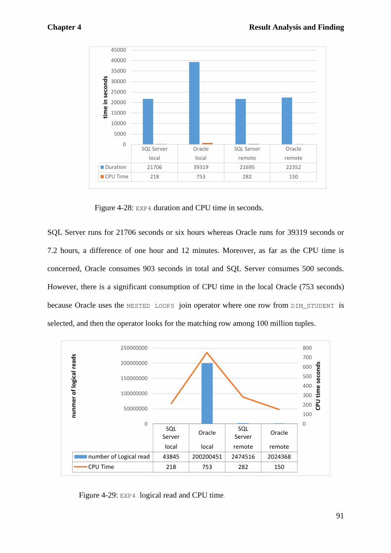
Chapter 4 Result Analysis and Finding
91
Figure 4-28: EXP4 duration and CPU time in seconds.
SQL Server runs for 21706 seconds or six hours whereas Oracle runs for 39319 seconds or
7.2 hours, a difference of one hour and 12 minutes. Moreover, as far as the CPU time is
concerned, Oracle consumes 903 seconds in total and SQL Server consumes 500 seconds.
However, there is a significant consumption of CPU time in the local Oracle (753 seconds)
because Oracle uses the NESTED LOOPS join operator where one row from DIM_STUDENT is
selected, and then the operator looks for the matching row among 100 million tuples.
Figure 4-29: EXP4 logical read and CPU time.
SQL Server Oracle SQL Server Oraclelocal local remote remote
Duration 21706 39319 21695 22352CPU Time 218 753 282 150
0
5000
10000
15000
20000
25000
30000
35000
40000
45000
time
in se
cond
s
SQLServer Oracle SQL
Server Oracle
local local remote remotenumber of Logical read 43845 200200451 2474516 2024368CPU Time 218 753 282 150
0
100
200
300
400
500
600
700
800
0
50000000
100000000
150000000
200000000
250000000
CPU
tim
e se
cond
s
nunm
er o
f log
ical
read
s

Chapter 4 Result Analysis and Finding
92
Figure 4.29 shows a significant difference with respect to logical reads between all VMs.
Accompanied by a high CPU time, the local Oracle outnumbers local SQL Server VM in
terms of logical reads. This situation is caused by the use of the NESTED LOOPS join operator.
If one examines the local SQL Server CPU time and logical reads, the MERGE JOIN operator
is faster than NESTED LOOPS and does not create many logical reads. The CPU consumption
of local SQL Server is still relatively high (218 seconds) compared to the remote CPU time
(282 seconds) where a SORT operator is used. Moreover, when the CPU time of both VMs are
compared, it can be seen that SQL Server consumes more CPU time than Oracle. This is
because Oracle does not use the SORT operator.
The above discussion explains some causes for the performance variations in EXP4.
Physical reads are an important factor to take into consideration as outlined in Figure 4.30.
Figure 4-30: EXP4 physical reads and average I/O latency.
As is the case in previous experiments, physical reads continue to create overhead on EXP4
runtime. Figure 4.30 shows that for EXP4 there are more physical reads than in EXP3, which is
reflected in the average I/O latency in all VMs. This situation is influenced by b the cloud
environment, for example, the local SQL Server experiences more physical reads in EXP4
(44316) than in EXP3 (7523). Therefore the average I/O latency jumps from 45 ms in the
SQL Server Oracle SQL Server Oraclelocal local remote remote
number of physical read 44316 988 2523460 2019541Avg I/O latency ms 56 14 15 15
0
10
20
30
40
50
60
0
500000
1000000
1500000
2000000
2500000
3000000
Ave
I/O
late
ncy
num
ber o
f phy
sica
l rea
ds

Chapter 4 Result Analysis and Finding
93
latter case to 56 ms in the former case. But the local Oracle instance experiences a decreasing
average I/O latency (14 ms) and the number of physical reads is 988 compared to the EXP3
when it has to wait for an average of 33 ms per physical read and the number of its physical
reads is 3786. The same applies to remote VMs. EXP4 also runs for a longer time than EXP3
and the average I/O latency is a contributing factor.
Finally, wait events in EXP4 provide further evidence that network creates
performance issues for RDBMS’ in CDD.
Figure 4-31 : EXP4 SQL Server wait events.
Figure 4.31 illustrates that waiting for the parallelism operation to finish takes longer time
than other waits (65.21%). The increase in the time required means that the parallelism is
accumulating time while waiting for threads to produce tuples. However, part of this wait is
caused by the parallelism manager, which waits for operations and produces CXPACKET5. This
wait would be of concern if it were combined with other larger waits such as
PAGEIOLATCH_SH where threads are waiting for the data to be placed in buffers.
5 “Occurs with parallel query plans when trying to synchronize the query processor exchange iterator” (SQL Server, 2015f).
45.99
65.21
16.24
%runtimelocal OLEDB
Remote CXPACKET
RemoteASYNC_NETWORK_IO
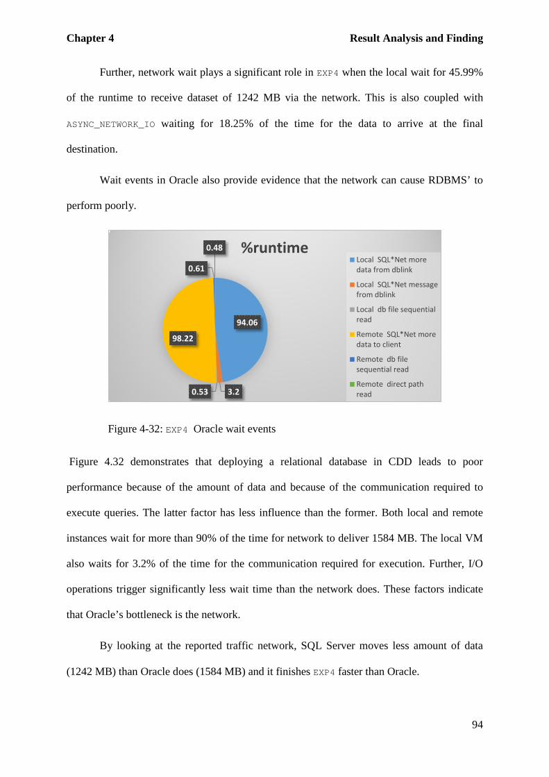
Chapter 4 Result Analysis and Finding
94
Further, network wait plays a significant role in EXP4 when the local wait for 45.99%
of the runtime to receive dataset of 1242 MB via the network. This is also coupled with
ASYNC_NETWORK_IO waiting for 18.25% of the time for the data to arrive at the final
destination.
Wait events in Oracle also provide evidence that the network can cause RDBMS’ to
perform poorly.
Figure 4-32: EXP4 Oracle wait events
Figure 4.32 demonstrates that deploying a relational database in CDD leads to poor
performance because of the amount of data and because of the communication required to
execute queries. The latter factor has less influence than the former. Both local and remote
instances wait for more than 90% of the time for network to deliver 1584 MB. The local VM
also waits for 3.2% of the time for the communication required for execution. Further, I/O
operations trigger significantly less wait time than the network does. These factors indicate
that Oracle’s bottleneck is the network.
By looking at the reported traffic network, SQL Server moves less amount of data
(1242 MB) than Oracle does (1584 MB) and it finishes EXP4 faster than Oracle.
94.06
3.20.53
98.22
0.61
0.48 %runtimeLocal SQL*Net moredata from dblink
Local SQL*Net messagefrom dblink
Local db file sequentialread
Remote SQL*Net moredata to client
Remote db filesequential read
Remote direct pathread

Chapter 4 Result Analysis and Finding
95
4.2.5 Experiment 5
In the experiments above, different factors were observed contributing to the poor
performance of RDBMS in CDD, including network and query execution approaches. EXP1
and EXP2 run for shorter times because the queries are relativity simple and there was less
data to traverse the network. EXP3 was more complicated, particularly in Oracle, since Oracle
required the specified data be brought to local VM before processing them. SQL Server, on
the other hand, performed EXP3 remotely and then sends only the result. Further, although
EXP4 involves joining only two tables with an inner join type without using any filtering
condition, the selected join operators involved in the queries took a long time to run.
Section 3.5.5 established that this experiment aimed to examine the performance of
RDBMS’ in CDD under different join types and also using WHERE clause. The following
figures show a snapshot of query results.
Figure 4-33: Snap shot of EXP5 results

Chapter 4 Result Analysis and Finding
96
4.2.5.1 Execution plans
Oracle (O)
Full table scan (Dim_Enrolment_Type)
SQL Server (S)
Clustered index scan (Dim_Enrolment_Type).(PK_Dim_Enrolment)
R
Hash match outer Do tuples meet hash condition?
Discarded tuples
NO
Select Yes
R
Merge Join(Left outer join)
Do tuples meet join condition?
Discarded tuples
NO
Select Yes
Figure 4-34: EXP5 local execution plans.
Figure 4.34.S shows that SQL Server continued to choose the MERGE JOIN operator, as was
the case in two out of four experiments even though there were 100 million tuples to join.
The implications for performance are significant especially where Oracle chooses the HASH
JOIN operator (see the O component of Figure 4.34.O) to perform the same experiment.
The remote execution plan shown in the S component of Figure 4.35 reveals that, yet
again, SQL Server sorts the data so that the MERGE JOIN operator can be executed. This sort
means that 100 million records will be sorted.

Chapter 4 Result Analysis and Finding
97
SQL Server (S)
Full table scan (child table)
Sort operator
Parallelism(Gather streams) Select
Oracle (O)
Full table scan (child table) Parallelim Select
Figure 4-35: EXP5 remote execution plans.
EXP5 executes in the remote Oracle VM (see Fig. 4.35.O) by scanning the table in parallel
and sending tuples to the requested instance. This scanning is done in full, which means that
same tuples are being touched at least once.
4.2.5.2 Comparison between RDBMS’
Execution plans show differences in terms of how they handle the execution of EXP5. For
instance, Figure 4.35 shows that although SQL Server consumes a higher CPU time in the
local instance, it still takes less time than Oracle. SQL Server needs 14993 seconds (four
hours and 16 minutes) whereas Oracle takes 20268 seconds (six hours and three minutes).
Figure 4-36: EXP5 duration and CPU time in seconds.
SQL Server Oracle SQL Server Oraclelocal local remote remote
Duration 14993 20268 14983 13406CPU Time 142 99 209 52
0
50
100
150
200
250
0
5000
10000
15000
20000
25000
CPU
tim
e
Dura
tion
Duration CPU Time

Chapter 4 Result Analysis and Finding
98
As far as CPU time is concerned, Oracle takes less time than SQL Server. This is because
SQL Server’s choice of MERGE JOIN operator creates the need for SORT operator to be used.
Figure 4.36 shows that SQL Server has high CPU consumption. This pattern also appeared in
EXP4 which indicates that while MERGE JOIN operator is the best choice from the optimiser’s
point of view, it provokes the need for a SORT operator to be used and this consumes more
CPU time than when a HASH JOIN operator is used.
EXP5 shows how both systems carry out the experiment, as well as how they differ in
terms of physical I/O operations, as shown in Figure 4.37.
Figure 4-37: EXP5 physical reads and average I/O latency.
In previous experiments, EXP3 and EXP4, although remote instances conduct high I/O traffic,
their average I/O latency was not as high as in local instances, where there were significantly
fewer I/O operations. This pattern also appears in EXP5 (see Figure 4.37) where it can be
seen that local VMs suffer higher average I/O latency than remote VMs. Conversely, it shows
a correlation between high average I/O latency and duration. EXP4 takes longer to run, and a
contributing factor to the increased runtime is that in the local SQL Server the instance
experiences high average disk response latency (56 ms per read).
SQLServer Oracle SQL
Server Oracle
local local remote remotephysical reads 3 5 2474178 2014059Avg I/O latency ms 25 23 18 15
051015202530
0500000
10000001500000200000025000003000000
Ave
I/O
late
ncy
num
ber o
f phy
sica
l rea
d
physical reads Avg I/O latency ms

Chapter 4 Result Analysis and Finding
99
Wait events differ in both systems, although network-related wait events appear to be
overwhelming.
Figure 4-38: EXP5 SQL Server wait events.
Figure 4.38 shows that SQL Server waits for the network to deliver 823 MB of data in both
instances: the local VM waits for 25% of the runtime whereas the remote instance waits 12%
for data to arrive from the local VM. In EXP4, network-related waits are higher than in EXP5
indicating that the latter receives a smaller amount of data. This is because in EXP4 there are
more columns requested from MYTABLE than in EXP5.
25.39
50.12
12.51
%runtime
local OLEDB
remote CXPACKET
remoteASYNC_NETWORK_IO

Chapter 4 Result Analysis and Finding
100
Also, Oracle waits the longest time for the network, as shown in Figure 4.39.
Figure 4-39: EXP5 Oracle wait events.
A remote instance of Oracle waits for the majority of its time for 1019 MB of data to reach
their final destination (see Figure. 4.41). I/O operations create a decreased wait time in the
instance and, in total, they create less than 1% as waiting time. Likewise, the local instance
waits for the network to deliver data for almost 94% of the runtime. It also waits for 5% of
the time for communication with remote instance.
In EXP5, Oracle moves larger amount of data (1019 MB) than SQL Server and it takes
longer time to finish. Same situation occurs in EXP4.
4.2.6 Experiment 6
The preceding experiments, with complexity ranges from moderate to simple have provided
evidence that the cloud network causes relational database performance to be less than
desirable. This experiment is described in Section 3.5.6 and the following figure show a
snapshot of query results.
93.55
5.030.410.08
98.93
0.660.04
0.01
%runtime
local SQL*Net more datafrom dblink
local SQL*Net messagefrom dblink
local db file sequential read
local db file scattered read
remote SQL*Net more datato client
remote direct path read
remote db file sequentialread

Chapter 4 Result Analysis and Finding
101
Figure 4-40: Snap shot of EXP6 results
4.2.6.1 Execution plans
Oracle (O)
Table access full (Dim_student)
SQL Server (S)
Clustered index scan ( Dim_student).(PK_studnet Key)
R
Hash join Do tuples meet join condition?
Discarded tuples
NO
Select Yes
R
Merge join(inner join)
Do tuples meet join condition?
Discarded tuples
NO
Select Yes
Figure 4-41 : EXP6 local execution plans.
In four out of five experiments, SQL Server chose the MERGE JOIN operator, although the
choice led to sorting 100 million rows. However, Oracle chose to employ a HASH MATCH join.
The remote execution plans for EXP6 show that there is evidence explains how the
execution of queries by RDBMS’ in a cloud environment causes poor performance (see
Figure 4.41).

Chapter 4 Result Analysis and Finding
102
SQL Server (S)
Full table scan (child table)
Sort operator
Parallelism(Gather streams) Select
Oracle (O)
Full table scan (child table) Parallelim Select
Sample table scan (child
table)
Sample table scan (child table)
Full table scan (child table)
Sample table scan (child table)
Full table scan (child table)
Figure 4-42: EXP6 remote execution plans.
The O component of Figure 4.42 shows that a table scan has been performed but more
importantly, the SAMPLE scan in Oracle is carried out three times. This is surprising because
Oracle indicates that SAMPLE scan can only be used when SAMPLE clause is used in the
query, which is not the case here (Oracle, 2011). Looking back at the query text Oracle may
interpret the WHERE condition as SAMPLE clause so that it sends data to the remote VM for
execution, in addition to pulling the all tuples and applying a filtering condition locally. In
fact, local Oracle reports, for the first time in this research, that it has to wait for data that it
sends to reach remote instance. Whether this approach is effective or not, there is at least

Chapter 4 Result Analysis and Finding
103
associated network overhead from applying this method. In the SQL Server execution plan
Figure 42.S, since the SORT operator does not show any kind of warnings such as “OPERATOR
USED TEMPDB TO SPILL DATA….”. This indicates that the sorting occurs in memory.
4.2.6.2 Comparison between RDBMS’
With execution plans showing differences, the collected performance data demonstrate there
are in fact significant variations between both systems.
Figure 4-43: EXP6 duration and CPU time.
The differences are apparent in Figure 4.43. For instance, SQL Server runs faster than Oracle
with more than four hours of difference between them. CPU time in local VMs indicates that
the SQL Server choice of MERGE JOIN consumes more CPU time than does Oracle’s choice
of the HASH MATCH join operator. Moreover, it is clear that the use of the SORT operator leads
to a difference of 25 seconds between remote VMs. Oracle’s consumption of CPU time is
125 seconds, whereas SQL Server consumes 235 seconds of CPU time.
When joining tables, it matters how many tuples are to be joined and the choice of
join operator also matters. For example, in EXP6 the local SQL Server experienced an
SQL Server Oracle SQL Server Oraclelocal local remote remote
Duration 22353 37166 20208 22019CPU Time 226 210 235 125
0
5000
10000
15000
20000
25000
30000
35000
40000
seco
nds
Duration
CPU Time

Chapter 4 Result Analysis and Finding
104
increase in CPU consumption that is six seconds greater than in EXP5; to a large extent,
RDBMS’ appear to suffer from operating over cloud network. For example, SQL Server’s
choice of the MERGE JOIN operator appears to have added performance overhead and this is
especially important when it is a requirement for both inputs to be sorted. This choice occurs
in five out of six experiments. This is also evident when both systems run the same queries,
but Oracle uses the MERGE SORT JOIN operator only once where there was an ORDER BY
clause.
Up to this point, the variations in performance appear to be informing multiple facts
in relation to CC as well as the underlying infrastructure. EXP6 also faces the reality of
accessing shared computing resources, which cause the RDBMS’ to suffer, as shown in
Figure 4.44.
Figure 4-44: EXP6 physical operations and average I/O latency.
Note that the average I/O latency shown in Figure 4.44 reflects the average I/O latency per
read.
SQLServer Oracle SQL
Server Oracle
local local remote remotenumber of physical read 44316 38287 2523554 2019573write 0 0 80 0Avg I/O latency ms 54 27 59 38
0
10
20
30
40
50
60
70
0
500000
1000000
1500000
2000000
2500000
3000000
Ave
I/O
late
ncy
num
ber o
f phy
sica
l ope
ratio
ns

Chapter 4 Result Analysis and Finding
105
The remote SQL Server VM in Figure 4.44, shows that there are 80 physical writes, although
EXP6 does not ask for the updating of any tuples, and the SORT operator does not use a
temporary table on the disk. Therefore, it is difficult say what causes this result. Every write
takes 32 ms to finish on average. The in local SQL Server, the previous five experiments
show that the highest average I/O read latency was recorded in EXP5 as 25 ms but this
increased to 54 ms per read in EXP6. This result was coupled with an increase in the number
of physical reads: 44316 reads in comparison to 3 reads in EXP5.
Similarly, remote Oracle in EXP6 experiences higher average I/O latency: 38 ms
compared to EXP5 (23 ms). There is also an increase in the local VM average I/O latency to
27 ms from 18 ms. This increase occurs, at least partially, because there are more physical
reads in EXP6 than in EXP5. EXP6 runs for a longer time than EXP5, and also EXP6 experiences
higher average I/O latency. However, generally SQL Server experiences higher average I/O
latency than Oracle, but Oracle runs for a longer period of time. Such a situation raises a
legitimate question as to why this is always the case. Wait events may provide an answer.
Both systems wait for similar events as in above experiments. SQL Server especially
waits for the same events. Oracle does the same but there is one new wait event that does not
appear in the preceding experiments.

Chapter 4 Result Analysis and Finding
106
Figure 4-45: EXP6 SQL Server wait events.
In Figure 4.45, the wait for the parallelism operation appears high in the remote VM at
63.32% of the runtime. The remote VM also waits for the network to deliver the data for
nearly 16% of the time. Further, SQL Server transfers 2864 MB and the local instance waits
for a network related wait event, OLEDB, for 43.93%. Moreover, when combining related
network wait events, network-related wait events take 59.7% of the runtime. Figure 4.45
indicates a significant amount of runtime waiting for the network.
Further, EXP6 experienced a higher wait for parallelism in remote instances than
EXP5. This is because although both queries processed the same number of tuples, EXP6
requested more columns than EXP5. Figure 4.45 signals that parallelism is a cause of
performance issues, but in the absence of an index, this wait is treated as unavoidable since it
is possible that both queries would require a longer runtime without parallelism execution,
especially when there are 100 million tuples to process.
In EXP6 the wait events for Oracle also show that the network plays an important role
in degrading the performance of relational databases in CDD.
43.93
63.32
15.77
%runtimelocal OLEDB
remote CXPACKET
remoteASYNC_NETWORK_IO

Chapter 4 Result Analysis and Finding
107
Figure 4-46: EXP6 Oracle wait events.
The graph in Figure 4.48 provides more evidence that the network impacts the performance
of RDBMS’ in a CC environment. For example, the choice to perform the SAMPLE TABLE
operation three times incurs a network overhead of 0.06% of the runtime. Although this
overhead appears insignificant, it creates an associated network overhead as a result of the
communication required to do such table scans. The communication that occurred between
VMs during EXP6 consumes 3.42% of runtime. Such an overhead appears inevitable but the
overhead is not negligible especially, in a cloud network. Further, the wait for 2572 MB of
data to reach the local VM, which accumulates more than 90% of EXP6’s duration. Figure
4.46 also shows that I/O latency does not create such an overwhelming overhead as the one
created by the network. In total, the remote VM waits for only 0.57% of the runtime for I/O
operations to complete. Therefore, Oracle suffers significantly because of the network.
In EXP6, although SQL Server reports a higher network traffic (2864 MB) than
Oracle (2572 MB), it finishes faster than Oracle.such case is reported in EXP4, EXP5 and
EXP6. However, by looking at the data transfer rates collected and reported in Appendix C,
pp. 206-208, they suggest that SQL Server experience higher WAN transfer rate than Oracle.
95.71
3.420.06
99.04
0.51
0.04
0.02
%runtime local SQL*Net more data fromdblinklocal SQL*Net message fromdblinklocal SQL*Net more data toclientremote SQL*Net more data toclientremote direct path read
remote db file sequential read
remote db file scattered read

Chapter 4 Result Analysis and Finding
108
4.2.7 Experiment 7
As is usually the case in relational database practice, with no exception made for CCD, many
tables are joined to obtain result. The previous analyses demonstrate that there are
contributing factors to the effects of the cloud network on RDBMS’ performance. For
instance, in EXP3 Oracle requires the data to be brought from the remote VM to the local VM
so it can process them, but SQL Server does the opposite and runs for a shorter time. That
says, RDBMS’ performance issues increase in a cloud environment particularly when large
datasets are involved.
This experiment is described in Section 3.5.7 and the following figures show a
snapshot of query results.

Chapter 4 Result Analysis and Finding
109
Figure 4-47: Snap shot of EXP7 results
4.2.7.1 Execution plans
SQL Server (S)
Clustered index scan (Dim_Programme).(PK_Programme_Key)
R
Nested loops(inner join)
Do tuples meet join condition?
Discarded tuples
NO
Select
Clustered index scan (Dim_Intake).(PK_Dim_Intake)
Table spool (Lazy spool)
Yes
Merge join(Inner Join)
Do tuples meet join condition?
Yes
Discarded tuples
NO
Table access full (Dim_Intake)
R
Hash matchDo tuples meet hash condition?
Discarded tuples
Table access full (Dim_Programme)
NO
Yes
Hash matchDo tuples meet hash condition?
Discarded tuples
NO
Select Yes
Oracle (O)
Figure 4-48. EXP7 local Oracle execution plan.

Chapter 4 Result Analysis and Finding
110
Oracle used the HASH MATCH join operator twice to execute EXP7. First it joined the remote
table with DIM_INTAKE and then it joined the result with DIM_PROGRAMME using the same
operator. However, SQL Server chose to scan DIM_INTAKE table first to find rows after1990
and store them on a temporary file. According to SQL Server, table spool is created on
memory so that whenever “spool’s parent operator asks for a row, the spool operator gets a
row from its input operator and stores it in the spool, rather than consuming all rows at once”
(Microsoft, 2015h). This file can then be scanned by using NESTED LOOPS to probe for
matches of tuples that come from performing an index scan on DIM_PROGRAMM. The optimiser
thinks that it is better to find matching rows between parent tables first and then join the
result with incoming tuples from the remote table.
Remote execution plans appear to have maintained a similar plan as in previous
experiments. For instance, SQL Server sorts the data because it employs the MERGE JOIN
operator.

Chapter 4 Result Analysis and Finding
111
SQL Server (S)
Full table scan (child table)
Sort operator
Parallelism(Gather streams) Select
Oracle (O)
Full table scan (child table) Parallelism Select
Full table scan (child table)
full table scan (child table)
Figure 4-49: EXP7 remote execution plans.
Similarities appear between EXP6 and EXP7, although they both have different types of
condition operators. However, since an OR operator is used in EXP7, it processes more data.
The next section will discuss whether this difference has any implications.
4.2.7.2 Comparison between RDBMS’
Executing EXP7 was different to EXP5 and EXP6 in relation to how each local optimiser chose
to carry out the execution, as follows.

Chapter 4 Result Analysis and Finding
112
Figure 4-50: EXP7 duration and CPU time in seconds.
Figure 4.50 shows that Oracle appears to be slow in EXP7; it needed 20 hours to run the
experiment while SQL Server needed 10 hours, even though SQL Server consumed more
CPU time than Oracle in both VMs. Further, the CPU time required by SQL Server provides
more evidence that MERGE JOIN is not the best join option. By contrast, Oracle employs HASH
JOIN twice to join the data but burns 369 seconds of CPU time while SQL Server spends 392
seconds on CPU time. This does not mean that the optimiser performs below par but that its
choice of MERGE JOIN is less suitable because, on the one hand there are 100 tuples coming
from the remote instance to join and on the other hand, this operator needs sorted data in
order to function. Hence optimiser uses SORT operator in the remote VM.
As mentioned earlier, and confirmed by this result, the use of the SORT operator has a
significant overhead. It has also been demonstrated on the CPU time of the remote Oracle
VM, which is significantly less than the remote SQL Server CPU time. Overall, SQL Server
is still relatively faster than Oracle. This result can be explained when one examines where
both systems spend most of their time.Although the foregoing discussion has given reasons
for the fact that EXP7 ran for at least 10 hours, it is also important to study the I/O operations.
SQL Server Oracle SQL Server Oraclelocal local remote remote
Duration 34890 72535 34884 38775CPU Time 392 365 443 50
0
10000
20000
30000
40000
50000
60000
70000
80000
seco
nds

Chapter 4 Result Analysis and Finding
113
Figure 4-51: EXP7 I/O operations and average I/O latency.
The average I/O latencies in EXP7 were the highest. The local SQL Server continued its
pattern with a high average I/O latency of 208 ms per read. This contributes to the creation of
a long-running query, although 0 ms is reported as the average I/O latency per write. Its
remote VM experiences less average I/O latency than in EXP6 even though it does more
reads. Clearly the local SQL Server is affected by a poor cloud environment. Such variations
indicate inconsistencies in performance measures of RDBMS’. This conclusion can be
verified by looking at the local Oracle disk latency where Oracle experienced significantly
less average I/O latency than local SQL Server in all the experiments so far, suggesting that
variations in performance can occur within the same PuC service provider. In addition to
remote VMs that seem to always perform more physical reads the average I/O latency never
reached 208 ms.
Further, EXP7 in Oracle showed a different pattern even though it performed a greater
number of I/O in the remote instance than in EXP6 and the average latency per read is less
than in EXP6. The local instance, on the other hand, performed fewer I/O operations than
SQL Server Oracle SQL Server Oraclelocal local remote remote
physical reads 1246 961 2622482 4629901physical writes 20 0 99 0Avg I/O latency ms 208 13 14 16
0
50
100
150
200
250
0500000
100000015000002000000250000030000003500000400000045000005000000
Ave
I/O
late
ncy
num
ber o
f phy
sica
l ope
ratio
ns

Chapter 4 Result Analysis and Finding
114
EXP6 and the avenge latency dropped from 27 ms to 13 ms. This suggests that EXP7 took
longer than EXP6 due to other factors in addition to I/O operation.
Wait events also provide more evidence that cloud network affects RDBMS’. The
network still plays a central role with respect to this outcome.
Figure 4-52: EXP7 SQL Server wait events.
Figure 4.52 clearly shows that the local VM waits for 47% of its time for 8613 MB of data to
arrive through the OLEDB provider. When compared to EXP6 the instance waits for 43.93%,
indicating that there are larger datasets to come in EXP7. There is also wait time associated
with the network in the remote VM when it waits for 16.29% of runtime for the network.
Further, the wait for the parallelism operation appears to be slightly higher than same wait in
EXP6.
Oracle wait events, by contrast, show that the network is the primary cause of the
poor performance of the relational database. Oracle is inconsistent in how it handles the
execution of the query. For instance, Oracle normally requests data to be brought to local VM
before applying any further processing. But this is not always the case since in EXP6 the
optimiser sent data to the remote location for execution and does so in EXP7.
47.09
65.38
16.29
%runtime
local OLEDB
remote CXPACKET
remoteASYNC_NETWORK_IO

Chapter 4 Result Analysis and Finding
115
Figure 4-53: EXP7 Oracle wait events.
Figure 4.53 shows that Oracle sends data to the remote VM and so the system has to wait for
the network 0.1% of the runtime. Yet, Oracle takes 95% of the local instance to obtain 8198
MB it requested to execute EXP7. Such a situation demonstrates the effect of network on the
runtime, that is, the larger the dataset that travels the network, the longer the query will take
to finish. Evidently, the local instance is dominated with network-related wait events.
Similarly, the remote instance faces the same situation when it waits for 93% of runtime for
the data to arrive at local VM. Further, I/O operations consume little from the runtime of both
instances; for example, the local instance (in total) waits for 1.53% for them to complete.
4.2.8 Experiment 8
Up to this point, there have been multiple experiments that have differed in their degree of
complexity but using the same dataset. Foregoing comparisons have shown that, the effects
of cloud network appears to be a significant contributing factor to the poor performance of
RDBMS’ in CDD. Sorting large amounts of data, in particular, is an expensive task, but SQL
Server chooses the MERGE JOIN operator and this requires the data need to be sorted. This
outcome occurred in six out of seven experiments thus far. Experiments that were conducted
94.55
2.60.30.1
92.92
0.78
0.66
0.09
%runtimelocal SQL*Net more data fromdblinklocal SQL*Net message fromdblinklocal db file sequential read
local SQL*Net more data toclientremote SQL*Net more data toclientremote db file sequential read
remote db file scattered read
remote direct path read

Chapter 4 Result Analysis and Finding
116
on Oracle indicate that the use of the HASH JOIN operator requires less time than the MERGE
JOIN operator, suggesting that HASH JOIN is more time efficient than MERGE JOIN. The
following figures show a snapshot of query results.
Figure 4-54: Snap shot of EXP8 results
As described in Section 3.5.8, this experiment aims to fully join two large datasets
over the cloud network and then perform an ORDER BY operation. EXP8 in Oracle did not
complete due to what appeared to a network issue and because of this, the execution plans
were lost.
4.2.8.1 Execution plans
SQL Server (S)
Clustered index scan ( Dim_student).(PK_studnet Key)
R
Merge join(full outer join)
Do tuples meet join condition?
Discarded tuples
NO
Select Yes Sort(Warnings sign)
Figure 4-55: EXP8 local SQL Server execution plan.
As mentioned above there is no local execution plan therefore this section addresses local
SQL Server execution plan.
Figure 4.55 illustrates that SQL Server employs the MERGE JOIN operator. Figure
4.57 also shows that an issue exists in the SORT operator resulting from the request to sort a
large dataset. The warning sign is shown below.

Chapter 4 Result Analysis and Finding
117
Figure 4-56: EXP8 ORDER BY warning.
Figure 4.56 indicates that the available memory is insufficient to perform the ORDER BY
clause and so the disk is used. This leads to a situation where it is necessary to (a) read the
data from disk, (b) bring them into memory, (c) write them again to disk, (d) carry out the
sort there, and (e) then read the data again into memory. This intensifies I/O traffic the over
cloud network.
SQL Server (S)
Full table scan (child table)
Sort operator
Parallelism(Gather streams) Select
Figure 4-57: EXP8 remote SQL Server execution plan.
As previously explained, SQL Server employs the SORT operator to satisfy the requirement of
MERGE JOIN operator. The SORT operator sorts 100 million tuples.
4.2.8.2 Comparison between RDBMS’
This section is different from the previous sections because Oracle crashed in EXP8 and
performance data were lost, especially most of the local instance data. Therefore this section
contains incomplete comparisons. However, the section will also show how Oracle deals with
EXP8 under a different load.

Chapter 4 Result Analysis and Finding
118
Figure 4-58: EXP8 duration and CPU time in seconds.
Figure 4.58 does not indicate that Oracle runs faster than SQL Server; rather, it shows that the
instance crashes at the 44364th second from execution start, and that the CPU consumes 410
seconds in the local VM and 59 seconds in the remote instance. However, SQL Server runs
for the longest time so far and also consumes the highest CPU time. These results show there
is a significant increase in resource consumption. For instance, if one compares CPU time in
EXP7, the local SQL Server with the same VM in EXP8 then there is a considerable jump from
392 seconds to 424 seconds respectively, although ORDER BY is performed on disk. Part of the
reason for this outcome may be a greater number of logical reads in EXP8.
SQL Server Oracle SQL Server Oraclelocal local remote remote
Duration 59118 44364 58015 41373CPU Time 424 410 259 59
050100150200250300350400450
010000200003000040000500006000070000
CPU
tim
e
Dura
tion

Chapter 4 Result Analysis and Finding
119
Figure 4-59: EXP8 logical reads and CPU time.
For the first time in SQL Server, logical reads in the local instance almost reached 500000
reads and this is reflected in CPU time. Figure 4.59 also indicates that despite remote
instances performing more logical reads than local VMs, they consume less CPU time. Then
in the local Oracle instance, zero logical reads indicates there is no information obtained due
to the query crashing. Before this occurred, the instance spent 410 seconds as CPU time,
whereas the remote VM spent 59 seconds as CPU time. As already mentioned, part of this
low CPU consumption is due to the absence of a SORT operator.
It was becoming evident that shared cloud environment is a contributing factor in
situations especially when there is an extensive disk activity for the ORDER BY clause.
SQL Server Oracle SQL Server Oraclelocal local remote remote
number of Logical read 429115 0 2688681 4,049,424CPU Time 424 410 259 59
050100150200250300350400450
0500000
10000001500000200000025000003000000350000040000004500000

Chapter 4 Result Analysis and Finding
120
Figure 4-60: EXP8 I/O operations and average I/O latency.
Note that zeros for Oracle instances indicate no information was collected.
Physical reads as shown in Figure 4.60 are the highest yet, which is a reflection of fully
joining two big tables. The local SQL Server continued to experience high average I/O
latency (111 ms), but not as high as in EXP7 (208 ms). Similarly, the remote instance
performed more physical reads and it saw a small increase in its average latency from 14 ms
to 15 ms in EXP7. Further, remote Oracle VM reads more physical data blocks with a higher
average latency (40), which was higher than in EXP7.
Figure 4-61: EXP8 tempdb I/O operations and average latency
SQLServer Oracle SQL
Server Oracle
local local remote remotephysical reads 54329 0 2808983 4,644,618physical writes 111 0 144 0Avg I/O latency ms 72 9 15 40
01020304050607080
0500000
100000015000002000000250000030000003500000400000045000005000000
Ave
I/O
late
ncy
num
ber o
f phy
sica
l ope
ratio
ns
readtempdb
writetempdb
directpathwritetemp
directpathreadtemp
local SQL server local OracleNumbers 485010 484930 0 0Avg I/O latency ms 49 360 16 10
050100150200250300350400
0100000200000300000400000500000600000
Ave
I/O
late
ncy
num
ber o
f I/o
Ope
ratio
ns
Numbers Avg I/O latency ms

Chapter 4 Result Analysis and Finding
121
It appears that physical operations on the temporary database creates significant performance
bottleneck. As shown in Figure 4.61, the local SQL Server VM takes an average of 360 ms
per physical write and reading the data again takes an average of 49 ms per read. Unlike
Oracle which although number of I/O operations is not obtained, average I/O latency is
significantly less than SQL Server.
In relation to EXP8, the above discussion has shown that, in terms of communication
and query execution relational databases are affected by the network’s inadequacy.
Figure 4-62: EXP8 SQL Server wait events.
Yet, the network appears to consume almost half of EXP8’s time, as is the case when the local
instance spends nearly 48% of the time waiting for 3633 MB of data to come (see Figure
4.62). In the remote instance, the parallelism operation accumulates a high wait period but
given the number of tuples that go parallel, this appears unavoidable, especially when the
parallel manager accumulates a CXPACKET wait while waiting for processors to finish their
assigned work (see Figure 4.62).
The following wait events occurred before the EXP8 crashed in Oracle.
47.79
65.88
16.44
%runtime
local OLEDB
remote CXPACKET
remoteASYNC_NETWORK_IO

Chapter 4 Result Analysis and Finding
122
Figure 4-63: EXP8 Oracle wait events.
Figure 4.63 shows that more than 90% of both VMs time is spent waiting for the data to
move via the network. This is an indication that operating a CDD faces the challenge of an
unknown network and it is overwhelming, even surpassing the I/O latency effect.
When EXP8 crashed, the transaction logs of both instances revealed the following
“ORA-12170: TNS: CONNECT TIMEOUT OCCURRED”. Oracle defines this error in this way:
“The server shut down because connection establishment or communication with a client
failed to complete within the allotted time interval. This may be a result of network or system
delays; or this may indicate that a malicious client is trying to cause a Denial of Service
attack on the server” (Oracle, 2015g). EXP7 ran for a longer time without being timed out. In
addition, both instances reported that the other VM was where the time-out occurred, which
suggests that it does not have control of the network. This event has led to an incomplete
picture of Oracle’s performance in relation to EXP8. In an attempt to obtain data, the size of
the dataset was reduced to 10 million tuples from 100 million.
92.94
1.920.830.43
93.41
0.79
0.5
0.2
%runtimelocal SQL*Net more datafrom dblinklocal SQL*Net message fromdblinklocal direct path write temp
local direct path read temp
remote SQL*Net more datato clientremote db file scatteredreadremote db file sequentialreadremote direct path read

Chapter 4 Result Analysis and Finding
123
4.2.8.3 EXP8 Oracle second approach (OSA)
When Oracle did not finish EXP8, it produced uncertainty with respect to its performance in
this experiment and created a need for undertaking a different approach in order to perform it
on Oracle. The data size employed in the second approach was reduced from 18 GB with 100
million tuples to 10 million so that a smaller amount of data went through the network,
minimising the effect of the network on EXP8.
index fast full scan ( Dim_student).(PK_studnet Key)
R
Hash join(full outer)
Do tuples meet join condition?
Discarded tuples
NO
Select Yes Sort
View
Figure 4-64: EXP8 OSA local Oracle execution plan
In EXP8 OSA, Oracle performed the full join using HASH JOIN operator and the sort took a
place in disk (see Fig. 4.64).
Sample table scan (child table) Parallelism Select
full table scan (child table)
Sample table scan (child table)
full table scan (child table)
Figure 4-65: EXP8 OSA remote Oracle execution plan.

Chapter 4 Result Analysis and Finding
124
The reason behind the sample access type as cited in EXP7 is not known. The optimiser used a
sample table access when SAMPLE clause was not used (see Figure 4.65). Therefore, it was
difficult explain it further without more information.
Figure 4-66: EXP8 OSA duration and CPU time in seconds.
Figure 4.66 shows that OSA finished in 4548 seconds or one hour and 15 minutes. Therefore,
one can extrapolate that, based on this time, the same query with 100 million tuples would
take 140 hours to run, or more than five days.
As the execution plan shows, there is extensive disk activity to sort data, which
influences the runtime as follows.
Figure 4-67: EXP8 OSA I/O Operation and average I/O latency.
local remoteOracle Oracle
Duration 4,548 4,103CPU Time 51 12
0500
1,0001,5002,0002,5003,0003,5004,0004,5005,000
seco
nds
local remoteOracle Oracle
physical reads 901 2,019,546Avg I/O latency ms 16 24
0
5
10
15
20
25
30
0
500000
1000000
1500000
2000000
2500000
Ave
I/O
late
ncy
num
ber o
f phy
sica
l rea
ds

Chapter 4 Result Analysis and Finding
125
Figure 4.67 shows that the remote instance appeared to experience a high average I/O latency
per read of 24 ms, whereas the local instance, which read only the index table, needed 16 ms
per I/O read.
Figure 4-68: EXP8 Oracle temp I/O operation and average I/O latency.
As Figure 4.68 shows disk activity that for the ORDER BY clause. It indicates that each disk
write took an average of 39 ms and, for the read, it took an average of 9 ms to finish.
Although these times contributed to the runtime, they did not provide a complete picture
about the query. Thus, wait events are going to be outlined (See Figure 4.69).
direct path writetemp
direct path readtemp
localNumbers 58275 58287Avg I/O latency ms 39 9
051015202530354045
5826858270582725827458276582785828058282582845828658288
Ave
I/o
late
ncy
num
ber o
f I/O
ope
ratio
ns

Chapter 4 Result Analysis and Finding
126
Figure 4-69: EXP8 OSA wait events.
Oracle still shows that network continues to play a significant role in prolonging the
execution time. Although this wait takes almost 90% of the local instance runtime waiting for
187 MB of data to come via cloud network, it appears that the I/O operation to write to a
temp file play a role that is, DIRECT WRITE TEMP 6creates a wait of nearly 2% of the runtime.
However, reading this data again takes less than 1% of local instance runtime. The I/O read in
the remote instance creates a total wait of 1.35% of the runtime, while the remaining 98.15%
of its runtime is recorded as a wait for the data to reach the local instance. Therefore, the
network appears to be causing a bottleneck, even though the dataset size is reduced. This
constitutes evidence that relational database practices suffer from performance issues if they
are carried out in cloud environment.
6 This wait indicates that the instance is waiting for direct write operation to finish on temp file (Oracle, 2015f).
89.61
3.421.840.37
98.15
1.29 0.06
%runtime local SQL*Net more datafrom dblink
local SQL*Net message fromdblink
local direct path write temp
local direct path read temp
remote SQL*Net more datato client
remote direct path read
remote db file sequentialread

Chapter 4 Result Analysis and Finding
127
4.2.9 Experiment 9
With the aim of investigating relational database performance in CDD, this study has
conducted experiments that have involved a variety of conditions. The systems used perform
less well and this is due to influence from cloud network. Further, the processes of relational
databases where normally more than one table is joined, appear to be challenged, especially
over cloud architecture.
SQL Server appears to have different requirements in regards to update query. For
instance, the pattern observed in the above experiments such as EXP1 and EXP8 demonstrate
that (a) if there is a WHERE condition which is based in the remote table, then SQL Server
returns only those tuples which satisfy the condition, and (b) otherwise it sends all the tuples
for the requested columns to the local instance for further processing. However, SQL Server
handles the update query that is based on sub-query in a manner that leads to a lengthy query.
When this occurs, the query is cancelled and is redone differently.
4.2.9.1 Execution plans
There is no execution plan for the local SQL Server, since the query stopped after running for
24 hours and consequently data were lost. However, the local Oracle execution plan is as
follows:
Table full access (Child table )
R Dim_paper
Nested loops Do tuples meet join condition?
Discarded tuples
NO
Update Yes
Figure 4-70: EXP9 local Oracle execution plan.

Chapter 4 Result Analysis and Finding
128
Figure 4.70 shows that Oracle executed EXP9 in the remote instance, instead of locally as
happened in EXP8 and EXP7. Oracle scanned MYTABLE to obtain the request tuples and
applied NESTED LOOPS as the join operator to check whether they meet the condition that
appears in the subquery, and then Oracle updates them.
The remote execution plans is as follows:
Full table access (child table) Parallelism update
Figure 4-71: EXP9 remote Oracle execution plan.
Figure 4.71 is similar to Figure 4.70 in which MYTABLE was scanned to obtain the requested
rows and updated after they had been checked to ensure they met the condition. However,
SQL Server appeared to approach the process differently, as follows:
Figure 4-72: EXP9 remote SQL Server execution plan.
Please note that this execution was not redrawn using VISIO because it was not practical to
do so.
Figure 4.72 gives a picture as to how the query is handled in SQL Server. The use of the IN
clause means that the subquery is required to return a confirmation that the value of
PAPER_KEY in the tuple was equal to 13362. SQL Server uses KETSET CURSOR which can be

Chapter 4 Result Analysis and Finding
129
described thus: “The keys are built from a set of columns that uniquely identify the rows in
the result set. The keyset is the set of the key values from all the rows that qualified for the
SELECT statement at the time the cursor was opened” (Microsoft, 2015i). However,
MYTABLE does not have a primary key thus SQL Server will have to create primary key in
order to identify those tuples that are to be updated. That is, SQL Server has no alternative
but to create a temporary file with a primary key. Thus, the table scan returns two columns as
follows:
Figure 4-73: EXP9 table scan
The table scan retrieves two columns, which SQL Server renames as BMK1002 and CHK1003.
(See Figure. 4.73). These columns are then used to segment the data as follows:
Figure 4-74: EXP9 segment operation

Chapter 4 Result Analysis and Finding
130
According to SQL Server’s online book, the SEGMENT operation “divides the input set into
segments based on the value of one or more columns” (Microsoft, 2015s). The segmentation
can make tuples uniquely identifiable.
Moreover, SQL Server employs a SEQUENCE PROJECT operator as shown in Figure
4.75 which SQL Server describes as the “[sequence project that] adds columns to perform
computations over an ordered set” (Microsoft, 2015j). One of these computations is the use of
ROW NUMBER FUNCTION, which returns a sequential number to each tuple within a segment
(Microsoft, 2015k). This appears when SQL Server replaces segment 1044 column with a
new column (EXPR1006), as follows:
Figure 4-75: EXP9 sequence project.
Figure 4.76 below shows that tuples are then inserted into the clustered table, which
has a primary key (Microsoft, 2015l). This means that 100 million tuples are to be inserted
again and, with available memory being insufficient, this occurs on disk and creates a
considerable amount of I/O traffic.

Chapter 4 Result Analysis and Finding
131
Figure 4-76: EXP9 clustered index insert
Once the insertion is done, tuples are sent to the COMPUTE SCALAR operator, which appears to
redefine column names to technical names that the SQL Server understands, as follows:
Figure 4-77: EXP9 compute scalar.
The table originally contained 35 columns. However, Figure 4.77 shows there are now 36
columns after adding a primary key. Further, SQL Server employs the POPULATION QUERY
operator and the operator “populates the work table of a cursor when the cursor is opened”
(Microsoft, 2015m). This operator appears to feed the KEYSET cursor with tuples that are
now uniquely identified and need to be updated.

Chapter 4 Result Analysis and Finding
132
Since KEYSET CURSOR contains identifiable tuples, SQL Server needs to retrieve the
remaining columns. Thus, INDEX SEEK is performed on the newly table created and left join
it with the tuple obtained from the LOOKING UP operator (see Figure 4.78).
Figure 4-78: EXP9 RID lookup operator
Once the joining is done, SQL Server uses the FETCH QUERY operator that “retrieves a
specific row from a Transact-SQL server cursor” (Microsoft, 2015n). This appears to deliver
the retrieved tuple(s) to the KEYSET CURSOR. Once the inserting data into KEYSET CURSOR is
done, SQL Server starts to call SP_CURSORFETCH procedure, which fetches one buffer each
time (Microsoft, 2015o) and it does this because SQL Server handles the update row by row
by using KEYSET CURSOR.
The difference between both systems in regards to EXP9 appears significant,
especially for SQL Server, whose approach causes a slow-running query. This will be
discussed further, with evidence, in a later section.
4.2.9.2 Comparison between RDBMS’
EXP9’s execution plans demonstrate that the maintenance of data integrity can be an issue
when a large dataset is involved which suggests that a relational database becomes less
effective in such a situation. However, this is not entirely the case and evidently Oracle
behaves differently and its approach to EXP9 causes fewer complexities than those that occur

Chapter 4 Result Analysis and Finding
133
in SQL Server’s approach. This section therefore outlines data about the performance of both
systems, noting that the data with respect to SQL Server are incomplete.
Figure 4-79: EXP9 duration and CPU time in seconds.
The graph in Figure 4.79 does not indicate that Oracle finished EXP9 faster than SQL Server,
but rather it shows that the SQL Server keeps running for 86557 seconds or 24 hours before
the experiment was cancelled. However, Oracle takes 1357 seconds to run EXP9. Figure 4.78
also shows that the local Oracle instance consumed only 0.009 seconds of CPU time. Local
instance of SQL Server burned 166 seconds as CPU time.
Further, the remote Oracle VM is where the higher consumption of CPU time occurs.
SQL Server also appears to burn a significant amount of CPU time, which is very alarming
but, since the execution plan in Figure 4.72 shows the many steps that the execution goes
through, the increase in CPU time is obvious. Thus, many logical reads were performed as as
result of 87740 calls for a SP_CURSORFETCH procedure in order to carry out EXP9 in the
remote SQL Server VM. These calls occur within 24 hours. In terms of CPU time each call
consumes between zero and 15 ms.
SQL Server Oracle SQL Server Oraclelocal local remote remote
Duration 86554 1,357 0 1352CPU Time 166 0.009 882 239
01002003004005006007008009001000
0100002000030000400005000060000700008000090000
100000
CPU
tim
e
Seco
nds
Duration CPU Time

Chapter 4 Result Analysis and Finding
134
Figure 4-80: EXP9 logical reads and CPU.
Notably, the local SQL Server appeared to undertake a considerable number of logical reads
and it consumed 166 seconds of CPU time. Figure 4.80 illustrates the way EXP9 was carried
out. There appears to be communication occurring to check whether the PAPER_KEY which is
being updated equals the number that appears in WHERE clause. This does not occur in Oracle.
Oracle carried out EXP9 remotely which reduced network overhead on performance.
Physical and write reads can add further insights to understanding the situation of
EXP9, as follows:
Figure 4-81: EXP9 I/O operations and average I/O latency.
SQLServer Oracle SQL
Server Oracle
local local remote remotelogical reads 831865 9 373065421 11,248,000CPU Time 166 0.009 882 239
01002003004005006007008009001000
050000000
100000000150000000200000000250000000300000000350000000400000000
CPU
tim
e in
seco
nds
num
ber o
f log
ical
read
s
logical reads CPU Time
SQLServer Oracle SQL
Server Oracle
local local remote remotephysical reads 0 2 2325815 8582166physical writes 1083 0 360075 2,306,460Avg I/O latency ms 35 8 8 14
0510152025303540
0100000020000003000000400000050000006000000700000080000009000000
10000000
Ave
I/o
late
ncy
num
ber o
f I/O
ope
ratio
n
physical reads physical writes Avg I/O latency ms

Chapter 4 Result Analysis and Finding
135
It is difficult to explain why SQL Server’s local instance has to perform physical writes,
although it is normal practice for a physical write to occur when the update happens. This is
concerning because the subquery returns one tuple from DIM_PAPER table which does not
normally cause any need for a physical write. However, as this instance is where EXP9
originates from, then physical writes are probably because SQL Server keeps a record in its
transaction log of those updates that are occurring in the remote instance. Further, physical
writes that occur in the Oracle remote instance are a result of the update statement (See
Figure 4.81). The same applies to SQL Server when it performed 630075 physical writes
before the cancellation. Moreover, the average I/O latency shown in Figure 4.81 reflects only
an average read latency; average write latency in the remote instance is 26 ms for SQL Server
and 21 ms for Oracle per write.
The approach that SQL Server employs in EXP9 leads to an extensive use of a
temporary database because the data volume is 18 GB. Therefore, it has to use the disk to
insert them into a clustered index table, as follows:
Figure 4-82: EXP9 TEMPDB I/O Operations and average latency.
While the number of physical reads is higher, as shown in Figure 4.82, its average I/O latency
is less than 10 ms. However, physical writes have a high I/O latency per write.
Physical reads Physical writesNumbers 422152 302688Avg I/O latency ms 8 44
05101520253035404550
050000
100000150000200000250000300000350000400000450000
Ave
I/O
late
ncy
num
ber o
f I/O
ope
ratio
ns
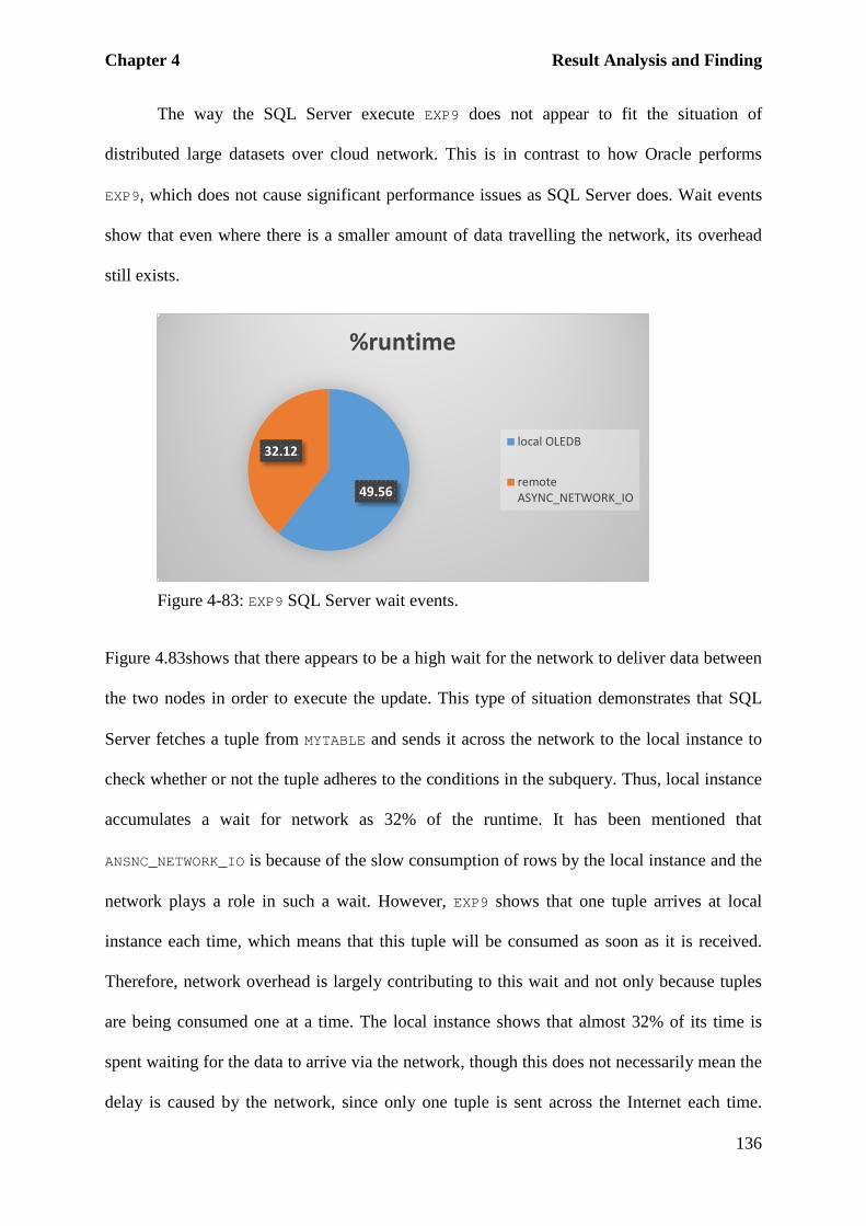
Chapter 4 Result Analysis and Finding
136
The way the SQL Server execute EXP9 does not appear to fit the situation of
distributed large datasets over cloud network. This is in contrast to how Oracle performs
EXP9, which does not cause significant performance issues as SQL Server does. Wait events
show that even where there is a smaller amount of data travelling the network, its overhead
still exists.
Figure 4-83: EXP9 SQL Server wait events.
Figure 4.83shows that there appears to be a high wait for the network to deliver data between
the two nodes in order to execute the update. This type of situation demonstrates that SQL
Server fetches a tuple from MYTABLE and sends it across the network to the local instance to
check whether or not the tuple adheres to the conditions in the subquery. Thus, local instance
accumulates a wait for network as 32% of the runtime. It has been mentioned that
ANSNC_NETWORK_IO is because of the slow consumption of rows by the local instance and the
network plays a role in such a wait. However, EXP9 shows that one tuple arrives at local
instance each time, which means that this tuple will be consumed as soon as it is received.
Therefore, network overhead is largely contributing to this wait and not only because tuples
are being consumed one at a time. The local instance shows that almost 32% of its time is
spent waiting for the data to arrive via the network, though this does not necessarily mean the
delay is caused by the network, since only one tuple is sent across the Internet each time.
49.56
32.12
%runtime
local OLEDB
remoteASYNC_NETWORK_IO

Chapter 4 Result Analysis and Finding
137
This implies that this will accumulate a network wait whether or not the data are actually
travelling the network or the data are not yet on the network.
Oracle demonstrates a similar pattern about network overhead on performance, as
follow:
Figure 4-84: EXP9 Oracle wait events.
In previous experiments, the wait for data to arrive is overwhelming because there is actually
data crossing the network. However in EXP9, the network wait indicates that the local
instance is waiting for acknowledgment from remote VM. This is a normal wait, since Oracle
executes EXP9 remotely and the local instance accumulates time as it waits for the update to
finish. However, by totalling up I/O operation waits in remote VM, it shows that the VM
spends the majority of the runtime (45%) in I/O operations. Therefore, I/O is Oracle’s
bottleneck in EXP9.
However, it is nearly impossible to determine in SQL Server where most performance
issues come from although from the way it handles EXP9, issues exist. A different approach
was undertaken in order to investigate further SQL Server’s approach to updating queries.
This includes removing the subquery and instead choosing the PAPER_KEY value once from
46.23
4.364.16
25.95
17.02
1.91
%runtime local SQL*Net message fromdblink
local db file sequential read
local db file scattered read
remote db file scattered read
remote db file sequential read
remote direct path read

Chapter 4 Result Analysis and Finding
138
DIM_PAPER and passing it to an update procedure located in the remote instance. This ensures
that the two tables are indirectly joined.
4.2.9.3 Exp9 SQL Server second approach (SSSA)
The execution plans for both VMs are as follows:
Figure 4-85: EXP9 SSSA localSQL Server execution plan.
As shown in Figure 4.85, SQL Server performs Clustered Index Seek to get
PAPER_KEY that is to be updated from DIM_PAPER. It appears that SQL Server uses constant
scan operator as holder for the value of the parameter @PAPER_KEY (see Section 3.5.9, p. 64).
Table scan Parallelism
(Gather streams) Table update update
Figure 4-86: EXP9 SSSA remote SQL Server execution plan for different approach.

Chapter 4 Result Analysis and Finding
139
Figure 4-87: EXP9 SSSA table scan
Once the remote VM receives the PAPER_KEY value, SQL Server carries out a table scan to
obtain the requested tuples (See Figure 4.87). In other words, passing the value to table scan
filters out those tuples whose PAPER_KEY value does not correspond to 13362. Such
execution plans suggest that based on this approach, EXP9 will not take long to finish.
To find whether or not EXP9 SSSA is different from EXP9 with sub-query, one needs
to look at the following figure:
Figure 4-88: EXP9 SSSA duration and CPU time in seconds.
This approach results in a significant difference in performance (see Figure 4.88). By
removing the subquery, SQL Server runs for 500 seconds with less work occurring in the
SQL Server SQL Serverlocal remote
Duration 500 498CPU Time 0.03 27
0
5
10
15
20
25
30
497
497.5
498
498.5
499
499.5
500
CPU
in se
cond
s
dura
tion
in se
cond
s

Chapter 4 Result Analysis and Finding
140
local instance, and with only 30 ms of the runtime consumed as CPU time. Moreover, CPU
time in the remote instance shows a dramatic decrease from 884 seconds with the subquery to
only 27 seconds without it.
Figure 4-89: EXP9 SSSA I/O Operations and average latency.
The remote instance appears to handle most of the work in this approach, and it takes 33 ms
on average per read and 48 ms on average per write. The local instance continues to
experience an issue with its cloud environment and, although SQL Server performs only two
physical reads, it took 22 ms on average per read. Figure 4.89 indicates that it is not always
the case that when there are more physical reads, average I/O latency increases, but rather the
PuC plays an important role in affecting the time required for I/O operations to complete.
Such effects can be both negative and positive. For instance, while the remote instance
outnumbers the local instance in terms of the number of physical reads, its average I/O
latency ranges from 8 ms to 59 ms and, in the local instance, it experiences as high as 208 ms
average per read and as low as 12 ms.
This approach shows multiple differences and the wait events that occurred are also
different, as follows:
SQL Server SQL Serverlocal remote
physical reads 2 2325748physical writes 0 920824Avg I/O latency ms 22 33
0
5
10
15
20
25
30
35
0
500000
1000000
1500000
2000000
2500000
Ave
I/O
late
ncy
num
ber o
f I/O
ope
ratio
ns

Chapter 4 Result Analysis and Finding
141
Figure 4-90: EXP9 SSSA wait events
As shown in Figure 4.90, the remote instance waits for different wait events and, as an
example, 25% of runtime is spent on LATCH_EX. However, SQL Server defines this as
occurring “when waiting for an EX (exclusive) latch. This does not include buffer latches or
transaction mark latches,” (Microsoft, 2015f) which indicates that this wait event is not
related to I/O operation or data. Further, the remote instance waits for
ASYNC_IO_COMPLETIONT (14.56%) and, accompanied with PAGEIOLATCH_SH (25.15%), these
waits are disk-related waits because SQL Server defines ASYNC_IO_COMPLETIONT as
occurring “when a task is waiting for I/Os to finish” (Microsoft, 2015f) and PAGEIOLATCH_SH
as waiting for the data to be written into memory (Microsoft, 2015f). Therefore, with this
approach EXP9 is I/O bound.
21.1
21.1
26.04
25.15
15.12
14.56
%runtime
local MSQL_DQ
local OLEDB
remote LATCH_EX
remote PAGEIOLATCH_SH
remote CXPACKET

Chapter 4 Result Analysis and Finding
142
4.4 Findings
The aim of this research is to investigate relational database performance in a CC
environment using a non-optimised environment. Therefore, two RDBMS’ are chosen in
order to find out where the performance breakpoints are. The above analyses demonstrate that
relational databases as a data manipulation approach fall victim to two factors that cause them
to perform in a suboptimal manner. The first factor is the shortcomings in methods used by
RDBMS’ when executing queries over cloud network. These methods sometimes expose the
relational database to unnecessary network overheads. The second factor is that the PuC
environment creates a situation where poor performance observes in the relational database.
In conducting this research, nine experiments are created that any relational database
should be able to execute so that a variety of performance data could be obtained and
compared in an attempt to determine the factors that are involved in relational databases
becoming ineffective in operating in a PuC. Indeed, these experiments reveal significant
findings that are important for a wide range of stakeholders. The following sections outline
these findings.

Chapter 4 Result Analysis and Finding
143
4.3.1 Performance measures in Cloud Computing
The comparisons between both systems demonstrate an inconsistent pattern, as the relational
database performance is being evaluated in CDD. This is important because there are many
factors that play different roles, whether negative or positive.
Experiment System Local physical read
numbers
Local average I/O latency
ms
Remote physical read
numbers
Remote average I/O latency ms
EXP1 SQL Server 171 12 2439171 10 Oracle 890 10 2019840 6
EXP2 SQL Server 2145 27 2325816 12 Oracle 1453 11 2019474 8
EXP3 SQL Server 7523 45 2325789 10 Oracle 3786 33 2019573 14
EXP4 SQL Server 44316 56 2523460 15 Oracle 988 14 2019541 15
EXP5 SQL Server 3 25 2474178 18 Oracle 5 23 2014059 15
EXP6 SQL Server 44316 54 2523,554 59 Oracle 38287 27 2019573 38
EXP7 SQL Server 1246 208 2622482 14 Oracle 916 13 4629901 16
EXP8 SQL Server 54329 72 2808983 15 Oracle N/A N/A 4644618 40
EXP8 OSA Oracle 991 16 2020096 24 EXP9 SQL Server N/A 35 2325815 8
Oracle 2 8 8582166 14 EXP9 SSA SQL Server 2 22 2325748 33
Table 4-1: Average I/O latency V. number of physical reads.
Table 4.1 reflects PuC effect on RDBMS’ performance. RDBMS’ are known to be I/O bound
and in some experiments, such as EXP7, the local SQL Server average I/O latency reaches as
high as 208 ms per read, even though the number of physical reads is not as high as reported
in remote VM. In local instances, such as EXP9 SSSA, the instance undertakes two I/O reads
but the I/O latency is 21 per read. Similarly, the remote Oracle instance in EXP7 performs a
higher number of I/O than it does in EXP6 but average I/O latency is less than in EXP6. Table
4.1 indicates that there is no relationship between number of physical reads and high average
I/O latency in a CC environment.

Chapter 4 Result Analysis and Finding
144
Further, the experiments conducted for this study demonstrate different patterns in
regards to WAN overheads on performance. This results in a situation where both systems
appear to experience different levels of WAN overhead; for example, although SQL Server
transfers a higher volume of data in EXP6, it finishes before Oracle (see Table 4.2 below).
Experiment System Network traffic in MB
Runtime in seconds
EXP1 SQL Server 0.162 89 Oracle 10 115
EXP2 SQL Server 125 359 Oracle 21 258
EXP3 SQL Server 0.244 111 Oracle 1011 17420
EXP4 SQL Server 1242 21706 Oracle 1584 39319
EXP5 SQL Server 823 14,993 Oracle 1019 20268
EXP6 SQL Server 2864 22353 Oracle 2572 37166
EXP7 SQL Server 8613 34890 Oracle 8198 72535
EXP8 SQL Server 3633 59118 Oracle N/A N/A
EXP8 OSA Oracle 187 4548 Table 4-2: network traffic V. runtime
However, this is not always the case: in EXP2, SQL Server transfers a larger dataset and takes
longer time than Oracle. The table also shows that in EXP6 and EXP7, SQL Server transfers
lager datasets than Oracle but runs for a shorter time. In EXP7, SQL Server transfers the
largest datasets that it does in EXP8 but finishes faster. However more importantly, if the
network traffic does not stay under 22 MB, then the relational database will perform poorly.
Table 4.2 provides evidence that high network traffic does not always cause a long-
processing query.
Therefore, the experimental work in this study demonstrates that there is only one
performance measure that is consistent and this is only if the network traffic is 21 MB or less.
Table 4.1 and 4.2 indicate that performance measures that are employed exhibit varying

Chapter 4 Result Analysis and Finding
145
degrees of inconsistency. Therefore, H1 which states that there is no consistent measure of
performance when comparing RDBMS’ operating in CC is accepted.
4.3.2 Performance of RDBMS’ as CDD
This study considers that it is practical to deploy relational databases for large dataset tasks in
CDD. However, if they operate in a non-optimised environment then based on the foregoing
results their performance may not be desirable, especially in commercial environments where
tasks need to be finished in as short a time as possible. This does not appear to be achievable
unless more investments is made to optimise not only the hardware, but also the RDBMS’.
Further, although there is a perception that the database optimiser is smart, the cloud
environment network appears to intensify known difficulties of query optimisation in
distributed RDBMS’. The experiments conducted in this study reveal cases where the
decision-making regarding the choice of join operators leads to longer runtimes, and
significantly so in some cases. This choice of join operator is an important aspect in
improving performance, and EXP1 and EXP4 indicate that while both systems indicate that the
NESTED LOOPS join operator is the best choice if the joined data are not large and indexed,
Oracle employs it even though the incoming data are not indexed. This results in high CPU
consumption and contributes to both experiments taking longer time to run in Oracle than in
SQL Server. Among other factors, although SQL Server uses the SORT operator to index the
data implicitly, it consumes less CPU time and finishes faster.
Further, the results indicate that SQL Server is in favour of using the MERGE JOIN
operator and evidently, this occurs in seven out of nine experiments. That is, it is just EXP1
and EXP9 that SQL server does not use the MERGE JOIN operator. This operator requires all
inputs be sorted, which triggers the need to sort 100 million tuples every time the operator is
chosen. Oracle mostly uses the HASH JOIN operator and it causes Oracle to consume
significantly less CPU time. In addition, SQL Server’s remote instances have higher CPU

Chapter 4 Result Analysis and Finding
146
time than Oracle’s because the use of the SORT operator to satisfy the requirements of using
the MERGE JOIN operator. That indicates issues on the methods of query execution by SQL
Server in CDD.
Further, SQL Server executes EXP9 in a manner that causes a long-running query and
the highest CPU time of all nine experiments. That method does not well fit cloud
architecture. Evidently, when the subquery is removed in SSSA, the system does not display
performance issues. This is in addition to Oracle’s approach to EXP9, when Oracle does not
execute the query in the same way that SQL Server does and finishes in less time.
The findings indicate with known performance issues of distributed RDBMS’, these
shortcomings become magnified when RDBMS’ are deployed in CDD. Hence, multi-variate
data analysis is used to determine whether that there is any statistical evidence to support
these findings. A comparison of the two systems indicates that methods such as join operators
create performance issues in CDD if they are not used appropriately. To demonstrate this, the
following scatter plots are used.
Figure 4-91: SQL Server duration v. CPU time.

Chapter 4 Result Analysis and Finding
147
Figure 4.91 shows that there is a significant correlation between how RDBMS’ execute
queries in a CC environment and the increase in duration. For instance, in the top right of the
Fig 4.88, there is a cluster of 10 data points mostly located on the diagonal. At the bottom of
this cluster are points 9 and 10 (EXP5 local and remote VMs), and at the top of this cluster is
point 15 (local EXP8). All of these points show the effect of the decision made by the SQL
Server to use the MERGE JOIN operator, which triggers the need to use the sort operator.
Further, point 17 represents EXP9, where SQL Server consumes the highest CPU time
because of its implementation of EXP9 using the KEYSET CURSOR over cloud network. Point
19 shows EXP9 SSSA, and a large difference can be observed. Figure 4.92 (following) shows
the same data, but for Oracle.
Figure 4-92: Oracle duration v. CPU time
Figure 4.92 exhibits a different pattern from Figure 4.91, that is, the data points appear to be
randomly scattered around the diagonal. Figure 4.92 also shows that data point 7 (local EXP4)
is the longest CPU time among the experiments. Since the NESTED LOOPS join operator is
performed in non-indexed data, local EXP4 becomes the highest Oracle experiment in terms
of CPU time. Further, Figure 4.92 also shows that, with the MERGE JOIN operator, SQL
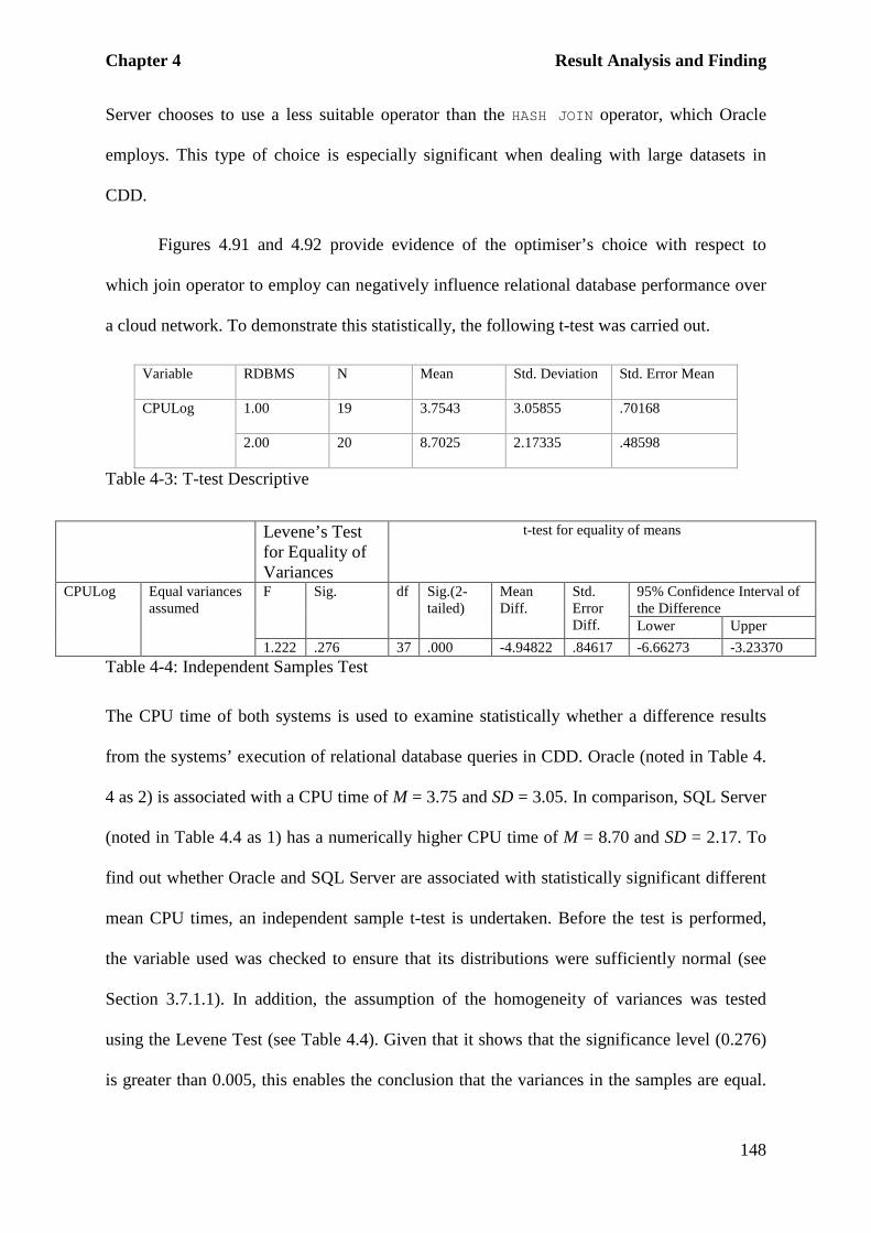
Chapter 4 Result Analysis and Finding
148
Server chooses to use a less suitable operator than the HASH JOIN operator, which Oracle
employs. This type of choice is especially significant when dealing with large datasets in
CDD.
Figures 4.91 and 4.92 provide evidence of the optimiser’s choice with respect to
which join operator to employ can negatively influence relational database performance over
a cloud network. To demonstrate this statistically, the following t-test was carried out.
Variable RDBMS N Mean Std. Deviation Std. Error Mean
CPULog 1.00 19 3.7543 3.05855 .70168
2.00 20 8.7025 2.17335 .48598
Table 4-3: T-test Descriptive
Levene’s Test for Equality of Variances
t-test for equality of means
CPULog Equal variances assumed
F Sig. df Sig.(2-tailed)
Mean Diff.
Std. Error Diff.
95% Confidence Interval of the Difference Lower Upper
1.222 .276 37 .000 -4.94822 .84617 -6.66273 -3.23370 Table 4-4: Independent Samples Test
The CPU time of both systems is used to examine statistically whether a difference results
from the systems’ execution of relational database queries in CDD. Oracle (noted in Table 4.
4 as 2) is associated with a CPU time of M = 3.75 and SD = 3.05. In comparison, SQL Server
(noted in Table 4.4 as 1) has a numerically higher CPU time of M = 8.70 and SD = 2.17. To
find out whether Oracle and SQL Server are associated with statistically significant different
mean CPU times, an independent sample t-test is undertaken. Before the test is performed,
the variable used was checked to ensure that its distributions were sufficiently normal (see
Section 3.7.1.1). In addition, the assumption of the homogeneity of variances was tested
using the Levene Test (see Table 4.4). Given that it shows that the significance level (0.276)
is greater than 0.005, this enables the conclusion that the variances in the samples are equal.

Chapter 4 Result Analysis and Finding
149
Further, the test shows that there is a statistically significant association, t value = -5.84, p =
0.000. The test indicates that SQL Server is associated with a statistically significant higher
CPU time than Oracle.
Further, there are cases where it has been demonstrated that the steps that the
RDBMS’ take to execute queries (for example, EXP9) generate I/O traffic that sometimes
cannot be understood. For instance, in EXP9, although updates occur in the remote instance,
the local SQL Server VM shows a high number of physical writes. Oracle does not cause
such operations, and neither does the second approach to EXP9. Therefore, for SQL Server, if
the updates do not occur in the local instance first, SQL Server keeps a record on the disk of
updates that take place in the remote instance. Even in experiments that do not aim to
perform modifications, SQL Server performs some physical writes. These can be seen in
EXP6, EXP7 and EXP8. Physical writes occur in EXP8’s local SQL Server instance and are
caused by performing ORDER BY clause on disk. However, in remote instances, the cause
behind these operations is not clear because while the SORT operator is in use, there are no
indications that SQL Server has to sort data on the disk. More importantly, these writes
perform in a shared and public cloud network which contribute to increase experiments’
runtime. Oracle, on the other hand, does not show any physical writes except in EXP8 and
EXP9.
In EXP7 and EXP8, Oracle uses SAMPLE table access, even though the SAMPLE clause is
not used. This study does not disagree with such use but it does indicate that this use affects
RDBMS’ performance over the cloud network by adding overhead related to I/O latency.
Oracle’s approach to EXP3 also affects performance since it requires a large dataset to travel
public and shared network in order to execute the query.

Chapter 4 Result Analysis and Finding
150
Therefore, the above discussion shows evidence from both the results side and from
the statistical perspective, that the query execution methods of RDBMS’ cause the systems to
work poorly in CDD when manipulating large datasets. This also leads to H2 which states
that “RDBMS’s execution of queries does not perform as expected when a large dataset is
distributed on a cloud network” being accepted, as the Sig. (2-tailed) value is less than the
significance level.
4.3.3 Influence of Public Cloud Computing network
This research is conducted on two different PuC systems using different workloads which
allows for the identification of their influence. The results indicate PuC environment is a
cause of performance for RDBMS’. For instance, SQL Server in EXP3 totals a wait of 12.43%
of the runtime for I/O operations to complete. Similarly Oracle in EXP2 and EXP9 reports a
total wait of 27.46% and 45% of the runtime for I/O reads to finish respectively. Further, the
local SQL Server instances generally experience a high average I/O latency, although they do
not process as large a dataset as the remote VM. However in this regard, Oracle, by contrast,
does not generally have a high average I/O latency. Sometimes the number of physical
operations in each system is close; however, average I/O latency is still high, as in the case of
EXP7, where the difference in physical reads in local instances is only 285 reads for SQL
Server, and the average I/O latency differs by 193 ms per read when compared to SQL Server
(see Table 4.1, p. 142).
Further, In EXP3, Oracle requires the data to be brought over the network before it
processes the query, although the count operation can be performed on the remote table. That
creates performance issues for RDBMS’ because of a lack of network capacity. Therefore,
EXP3 takes significantly longer to run in Oracle than in SQL Server (see Table 4.2, p. 143).
Further, in other experiments, Oracle demonstrates inconsistency in execution. In EXP7 and
EXP8 in particular, when, in addition to pulling the requested data to the local instance, it

Chapter 4 Result Analysis and Finding
151
sends some data to the remote instance as it does in EXP7. This approach increases CC
(WAN and I/O latency) overhead on performance.
The above results show that both systems wait for the network to deliver the requested
data, although network wait appears overwhelming in Oracle. SQL Server sometimes runs
faster, even when it transfers larger datasets, and this is reflected in wait-related events that
never go beyond 50% of the runtime. In comparison, Oracle never drops below 60%. This
situation is also evident in the 90 samples of DTR (see Appendix C, pp. 206-208), which
suggests that SQL Server uses what appears to be a faster network route.
To demonstrate the WAN effect in a statistical manner, the following tests are carried
out, namely, a correlation and simple regression.
Network traffic Log Duration Log Pearson Correlation .928**
Sig. (2-tailed) .000 N 16
Table 4-5: Correlation between Duration and Network Traffic
(**. Correlation is significant at the 0.01 level (2-tailed)
As Table 4.5 shows, there is a statistically significant correlation between duration and
network traffic. This relationship can be demonstrated as follows:

Chapter 4 Result Analysis and Finding
152
Figure 4-93: Duration v. network traffic.
The scatter plot shows that as network traffic increases, the duration also increases. It also
clusters experiments that transfer a high volume of data. It shows a linear trend, although
there are outliers in the lower left below the diagonal which represent data points where the
traffic size begins to exceed 100 MB (see Figure 4.93).
Further, a simple regression test produced the following result:
Coefficientsa
Model Unstandardised
Coefficients
Standardised
Coefficients
t Sig. 95.0% Confidence Interval for
B
B Std. Error Beta Lower
Bound
Upper Bound
1 (Constant) -4.887 1.462 -3.344 .005 -8.022 -1.753
networktrafficLog .692 .074 .928 9.325 .000 .533 .851
a. Dependent Variable: durationLog
Table 4-6: simple regression test
Table 4.6 indicates that the slope parameter is significantly different from zero at the level of
0.01. Thus, this is an important relationship between network traffic and duration. With 95%
confidence, Table 13 shows that with every unit increase in network traffic, there is an
increase in the duration between 0.533 and 0.851. Figure 4.94 (below) shows no major
departures from the straight line; therefore, the normality assumption is met.

Chapter 4 Result Analysis and Finding
153
Figure 4-94: Normality of simple linear regression test.
The foregoing discussion demonstrates multiple situations where the network overhead
appears and differs in a significant manner; it decreases only if less than 100 MB are
transferred. Also, Table 4.1, p. 142 provides evidence that the effect of PuC environment on
I/O latency is considerable. Therefore, the relational database that processes a large dataset is
constrained by the network, and it appears that the cloud computing environment is not the
best place for relational database deployment. Therefore, H3 is accepted: CC impacts
RDBMS’ due to network incapacities compared to n-tier architecture.
4.5 Conclusion
This research sought to test the following hypotheses:
H1: There is no consistent measure of performance when comparing RDBMSs operating in
cloud computing.
H2: RDBMS’s execution of queries does not perform as expected when a large dataset is
distributed on a cloud network.

Chapter 4 Result Analysis and Finding
154
H3: Cloud computing impacts RDBMSs due to network incapacities compared to n-tier
architecture.
Nine experiments have been conducted to identify potential breakpoints in relational
databases performance in CDD. The experimental scenarios have represented all cases that
the available dataset support. They range from simple (EXP1) to complex (EXP9) queries
which have different applications to the relational database. This range facilitates the
identification of the following break points:
1. RDBMS’ demonstrate inconsistencies in performance measures when operating in
CDD.
2. Both RDBMS’ performed less well than expected when they choose the less
optimal join operators, although SQL Server does this more than Oracle.
Therefore, RDBMS’ perform less adequately in a CC environment.
3. In a large dataset of 100 million tuples, the sort operator causes a significant
performance issue. SQL Server employs the SORT operator when it uses the
MERGE JOIN operator. Therefore, this indicates that the RDBMS’ are involved in
the poor performance of relational databases in CDD.
4. SQL Server executed EXP9 in a suboptimal manner by employing KEYSET CURSOR
in a CC environment and by undertaking physical writes in instances where it
does not have to. This indicates that SQL Server does not perform subqueries
efficiently in CDD. This behaviour is not observed when the subquery is removed.
Therefore, the subquery should not be included in an update query in SQL Server
if a large dataset is hosted in different locations over cloud network.
5. With distributed databases becoming more common in practice, the network
overhead should be kept to a minimum. However, Oracle does not appear to fully
realise this, and it still required a large dataset to traverse the network prior to the

Chapter 4 Result Analysis and Finding
155
execution of the experiments, although Oracle does apply this method in specific
cases (see EXP3). Therefore, methods of query execution by RDBMS’ lead to
poorly performing relational databases in CDD.
6. Network overhead becomes worse when more than100 MB of data travel through
the network. But this does not eventuate when the data volume is 21 or less MB.
7. PuC network is a source of performance issues because many users share the use
of the underlying infrastructure and the access to internal cloud network. This
effect is demonstrated in the difference in average I/O latency between local and
remote instances and I/O wait events. Oracle’s use of SAMPLE table access appears
to intensify such performance overhead.
These points indicate that even if the relational database operates in an optimised system, the
WAN overhead becomes significant and cannot be predicated once the traffic goes over 21
MB. Chapter 5 discusses the significance of these findings.

Chapter 5 Discussion
156
Discussion
5.0 Introduction
Chapter 4 provides detailed explanations for the experimental work that this research
undertakes, aimed at identifying performance issues of RDBMS’ in cloud-distributed
database. Chapter 5 presents the findings of this research in order to show their significance
to the research community and to those who develop RDBMS.
Section 2.3 demonstrates that further investigation is required to enhance
understanding of the application of RDBMS’ in data management. RDBMS’ are an effective
tool for data manipulation however the amount of data needing to be stored continues to
increase rapidly which creates new challenges for them. Relational databases have existed for
nearly 50 years; however, given the way they are implemented, systems such as NOSQL are
able to step in and take the attention in data management (see Section 2.1.2). Therefore, the
primary focus of the present study is to examine the performance of relational databases in
CDD when dealing with large datasets in order to determine whether the deployment of
RDBMS’ in CC leads to poor performance.
Notably, the results show an incremental pattern that indicates there is a main driver
behind this pattern, which is data volume, for example, Section 1.0 provides an extrapolated
data growth of around 7.2 zetabytes by 2015. In order to highlight processing and
management issues that contribute to RDBMS’ performance issues in CDD, nine experiments
have been performed on two RDBMS’ using a large dataset.

Chapter 5 Discussion
157
This research employs 18 GB and observes multiple cases where the performance
does not appear to be satisfactory. The results indicate that network overhead can only be
avoided if the network traffic is low and that the query optimisation implementation
approaches of RDBMS’ in CDD result in reduced performance. In addition the RDBMS’
used in the experiments exhibit varying and different problem areas.
This chapter contains 6 sections. This section which is the introduction of the chapter.
Section 5.1 discusses the findings of this research that are related to performance measure in
CDD. Section 5.2 clarifies on the findings in relation to RDBMS performance as CDD.
Section 5.3 explains the findings that are related to CC effects on RDBMS’ performance.
Section 5.4 provides a discussion of to explain the findings in relation to the difference
between the performance of RDBMS’ in cloud architecture compared to n-tier architecture.
Section 5.6 concludes Chapter 5.
5.1 Performance measures in Cloud Computing
This section discuss the finding that is related to RDBMS’ performance measures in CDD. It
also provides answer to research question 1 and 2.
This research assumes that RDBMS’ are originally developed to operate on n-tier
architecture, and it also assumes that these systems would have high performance if the same
experiments are carried out on such architecture. In this regard, CC creates different
challenges for RDBMS’ and based on the results presented in Chapter 4, they are negatively
affected. For instance, the findings indicate that although the experiments vary in how many
physical reads they require for execution, they differ significantly in average I/O latency. As
seen in EXP7’s local SQL Server, and this average contributes to prolonging the duration (see
Table 4.1, p. 142). I/O latency is a particularly significant factor to consider in relation to
technologies such as RDBMS’ because these systems are I/O bound. Moreover, EXP8 shows

Chapter 5 Discussion
158
extensive disk use, as RDBMS’ have to use it to perform the ORDER BY clause, which orders
100 million tuples in SQL Server (see Section 4.2.8). Even after the number of tuples is
reduced to 10 million rows, RDBMS’ order the data on the disk and, in both cases, this
occurs because of insufficient memory size. While the non-optimised environment is
intentionally used in this research, it reflects the situation of relational databases that have to
use disk/s when the shared, public environment combines to negatively affect performance.
Fortunately, as the remote instances perform higher significantly higher number of physical
reads but they do not experience as high average I/O latency as local instances, indicating
inconsistency between performance measures which is in line with the finding of Gunarathne
et al. (2010). Based on I/O latencies reported in Table 4.1, p. 142, experiments’ runtime
would be longer if remote VMs experience as high average I/O latency as local VMs.
The present study uses seven performance measures runtime, CPU time, disk
operations, average I/O latency, number of logical reads, network traffic and wait events
which enables it to form a more complete picture. These measure enable the research to
investigate the performance of RDBMS’ in CDD that deal with large datasets. For instance,
Kohler and Specht (2014) uses runtime, number of tuples returned as performance measures
and they indicate there is an associated overhead of table joins in a CC environment. Since
this study uses CPU time and compares it between two RDBMS’, it identifies the cause
behind such overhead (see Section 5.2 & Section 5.4 below). Also, the use of wait events,
average I/O and network traffic enables the present study to show the effects of cloud
infrastructure on performance (see Section 5.3 below). Therefore, this provides answers for
Q1: What are performance measures that can be applied to examine RDBMS’ performance in
CC? and Q2: Are the measures related to Q1 valid for measuring RBDMS’ in the cloud when
large datasets are being manipulated.

Chapter 5 Discussion
159
5.2 Performance of RDBMS’ as CDD
This section carries out discussions about the findings related to RDBMS’ performance in
CC, and it provides an answer to Q3.
Aimed at examining the performance of relational databases dealing with large
datasets in clouds, Chapter 2 outlines two propositions that reveal a significant body of
knowledge. They show evidence that either RDBMS’ need change or that new RDBMS’ are
created. However, the work reveals that to a large extent, RDBMS’ are involved in creating
performance issues, and given the current implementation approaches of relational databases,
they are not suitable for processing large datasets in CDD.
Large datasets are a reality and their size continues to increase. In Section 2.1.2 it was
stated that query optimisers do not appear to perform well in a distributed environment.
These results provide further evidence that RDBMS’ are not suitable for large dataset
processing in a distributed, cloud-based environment. Although RDBMS’ should provide the
best execution plan, this experimental work shows otherwise; instead, the chosen plans tend
to increase the performance overhead. If one examines the number of tuples that both systems
deal with in this research, in most cases the RDBMS’ do not provide acceptable performance.
For instance, in six out of nine experiments, SQL Server chooses the MERGE JOIN operator,
which does not appear to improve performance although the RDBMS vendor claims that it is
the fastest join operator. Likewise, Oracle’s choice of NESTED LOOPS in EXP5 appears to
contribute significantly to a long running query, although its choice of the HASH JOIN
operator appears to perform better than the MERGE JOIN operator.
Relational databases usually require two or more tables to be joined in order to
execute the task at hand, which becomes a challenge when a large dataset is involved. Unless
RDBMS’ deal with small datasets, as shown in EXP1 and EXP2, then they have difficulty

Chapter 5 Discussion
160
making joins. An important part of NOSQL design is that it avoids the joining of tables (see
Appendix E), which suggests that table joins create a performance overhead. This research
shows that RDBMS’ operating in CDD make inappropriate decisions that lead to this
overhead.
In addition, RDBMS’ choose execution plans that, instead of providing optimal
performance, these plans contribute significantly to degrading the performance. For both
systems, sorting data is an expensive task. This is important because large datasets are a
reality, and the systems appear to run less efficiently than is required for the purpose of large
dataset processing in a cloud-based environment.
The steps that SQL Server undertakes in EXP9, which uses KEYSET CURSOR (see
Section 2.4.9) indicates that including a sub-query in update statements in SQL Server causes
significant performance in a CC environment. More importantly, SQL Server perform
physical writes where it does not have to, especially when the query does not intend to update
the parent table and a cascade update is not required. Certainly, sub-queries in update
statements are not always an issue if they proceed in a manner that fits CDD as Oracle’s
approach. However, SQL Server’s approach to EXP9 does not fit CDD and this is evident this
appears when the sub-query is removed in EXP9 SSSA.
In EXP3, the system does not execute the aggregation query remotely, Oracle requires
data to be brought via the network from remote instance before continuing with the query.
Such decision becomes problematic in a CC environment since the network impedes the
performance of the systems. Thus, RDBMS’ operating in CDD face the challenge of unstable
Public Cloud network and they appear to cope less well.
This research supports Chen et al.’s (2010) claim that the relational data model
negatively impacts performance, because the findings of this research indicate that any

Chapter 5 Discussion
161
performance weaknesses in RDBMS’ are magnified when the system is installed in the cloud.
Moreover, this research’s findings are consistent with Batra and Tyagi (2012), Kohler and
Specht (2012), Durham, Rosen and Harrison (2014) and Sanders and Shin (2001), who
believe that there is an associated overhead with joining tables in RDBMS’, and that table
RDBMS’ do not efficiently perform table joins in CDD when large datasets are involved.
NOSQL performs better than RDBMS’ when no cross-reference is involved (see Appendix
E). Further, consistent with Kalnis and Papadias (2003) and Chaudhuri (2012b), this research
presents quantitative and statistical evidence that there are issues with the underlying
algorithms that choose the execution plans, and these issues make the systems unfit for the
purpose of processing large distributed datasets in a cloud-based environment.
Liu and Yu (1993) state that there is a need to investigate whether there is a role for
the RDBMS’ in choosing an unsuitable execution plan in distributed databases. The present
study indicates the problem is that execution plans are not optimised for distributed cloud
environments and significantly worsens the situation of RDBMS’ processing large datasets.
Consistent with Dokeroglu, Bayir and Cosar (2015), this research finds that sub-queries
create performance issues in CDD if they are carried out as SQL Server does in EXP9, and
that the way some RDBMS’ implement other queries (such as EXP3 in Oracle) as CDD
indicates that these systems have deficiencies.
These discussions reveal the evidence that (1) there appears to be issues with the
underlying algorithms that choose execution plans. These algorithms do not provide optimal
plans that fit CC environment and (2) there appears to be deficiencies with implementing
these plans in cloud environment. Therefore, Q3 which asks “what evidence exists that
RDBMS’ are creating significant performance issues in a cloud-computing environment” is
answered.

Chapter 5 Discussion
162
These evidence provide that current RDBMS’ are less useful in dealing with large
datasets in CDD. However, RDBMS’ have relatively reasonable performance when there is
no joining of large datasets, and when sub-queries are avoided in SQL Server. If H2 is
rejected, then RDBMS’ perform with no issues as CDD, and manipulating data of any
volume poses no major challenges.
5.3 Influence of Public Cloud Computing network
The results of the examination of RDBMS’ performance indicate that RDBMS’ do not
perform well when dealing with large datasets in a CC environment. Conducting experiments
of CDD using large datasets is a time-consuming task and produces long-running queries.
Importantly, the results reveal that data movements across nodes in a cloud environment
should be kept to a minimum otherwise RDBMS’ performance cannot be predicted.
In line with Kohler and Specht (2014), Durham, Rosen and Harrison (2014) and
Thakar et al. (2011), the network overhead becomes significant as the data size increases.
Further, this research reveals that relational databases do not display performance issues
when the size of the dataset travelling the network is 21 MB or less. This is consistent with
Kohler and Specht (2014) whose dataset is not as large as the data size employed in the
current study. The authors show evidence that they do not observe similar performance issues
when their experimental work is conducted off the cloud.
This research agrees with Hacigumus et al. (2010) in that relational database
deployment in the cloud requires further investigation to solve the issues that lead to the
current situation. It also agrees with Liu, Xia, Shroff and Zhang (2013) in that RDBMS’ do
not fit the purpose of large dataset manipulation in a cloud-based environment. The causal
relationship examined in the present study provides evidence that there is a significant

Chapter 5 Discussion
163
correlation between network traffic and runtime. In addition, a simple regression test shows
that the model explains 0.86 of the data variation.
Businesses usually want to receive a response as soon as possible, and based on the
environments employed in this research, this does not happen. The findings do not agree with
those of Minhas et al. (2008), because although they conclude that there is an overhead in I/O
performance associated with running databases in clouds, such overhead is 10% or less of the
runtime. This research demonstrates that the overhead is quite significant when a large
dataset is being manipulated. For instance, Oracle VMs in EXP2 and EXP9 and SQL Server
in EXP3, the overhead of cloud environment on I/O performance is 27.46%, 45% and 13.43%
of runtime respectively. Table 4.1, p. 142 shows that local SQL Server VM in EXP7
performed 1246 physical reads with an average latency of 208ms per read. This means that
the total average is four minutes. The table also demonstrates that the systems perform over
two million physical reads in EXP6 and the average I/O latency is 59 ms for SQL Server and
38 ms for Oracle. These results are consistent with Thakar et al. (2011) who indicate that PuC
environment affects the performance of RDBMS’ in terms of I/O latency and in line with Li,
Yang, Kandula and Zhang (2010), who find high variations in performance between different
public providers.
Add to that, a number of previous works examine whether virtualisation software
affects the performance of different database systems using benchmarking tools (see Section
2.4.2). The findings of this research indicate that measuring relational database performance
using tools that are not originally developed for CC does not draw a complete picture, which
is in line with the findings of Curino et al. (2011) and Binnig et al. (2009).
Although the present study relies on secondary data because of its limitation in terms
of the difference between performance in and off the cloud, the research indicates CC
negatively influences RDBMS’ manipulation of large datasets and results in significant

Chapter 5 Discussion
164
performance issues when the data travel across the Internet. A shared and PuC environment
also impacts RDBMS’ performance negatively especially when RDBMS’ are I/O bound.
These points therefore, answers Q4 that asks “What influence does CC have on relational
database performance” and provide evidence that RDBMS’ as CDD are not only I/O bound
but also become network bound.
If H3 is rejected then this means that there are no major issues in the cloud network
and that any large dataset can traverse the network with fewer problems and average I/O
latencies are shorter than reported in Table 4.1, p. 142.
5.4 Cloud architecture VS n-tier architecture
This research relies on secondary research that show RDBMS’ generally perform better on n-
tier architecture.
Section 1.0 explains the aim of this thesis; that CC creates a different environment for
RDBMS’ and this work is undertaken to test their performance in such an environment. As
Section 1.0 indicated, distributed RDBMSs normally deploy over n-tier architecture on
specifically designed infrastructure and that they connect their nodes on server(s) using
significant network bandwidths. Despite this, distributed RDBMS’ still suffer from
performance issues and this is before CC existed (see Section 2.2.3). PuC architecture on the
other hand, provides a shared pool of computing resources that provide alternatives to n-tier
architecture and also relies on shared and limited bandwidths, for both internal and external
networks (see Section 1.0 and Section 1.1). Figure 4.91, p. 145 and Figure 4.92, p. 146
represent the performance of the RDBMS’ query execution plan choices and implementations
over the PuC network where they demonstrate significant differences between the systems.
An independent t-test (see Table 4.4, p. 147) also shows that SQL Server is associated with a
higher CPU time than Oracle that is statistically significant. Table 4.1, p. 142 also indicates

Chapter 5 Discussion
165
the effect of public and shared environment on I/O performance using average I/O latency.
The situation observed in Oracle’s handling of EXP3 also points to the difficulties that the
RDBMS’ faced when operating in CDD. Add to that the effect of WAN on performance,
which is represented by the causal relationship between network traffic and the experiments’
runtimes (see Table 4.5, p. 150).
Section 2.3.2 provides proposals aimed at making RDBMS’ fit for cloud deployment.
In line with Thakar et al. (2011), Bose, Mishra, Sethuraman and Taheri (2009), and Kohler
and Specht (2014) whose studies show that RDBMS’ run better on n-tier architecture. And,
consistent with Dokeroglu, Bayir and Cosar (2015) who propose new algorithms to help
cloud relational databases make better choices when creating execution plans, the results of
this investigation indicate that since CC architecture is different from n-tier architecture,
RDBMS’ that appear to have been developed originally to operate on n-tier architecture are
not performing optimally. This explains why any issues with distributed RDBMS’ are
intensified in CDD. This also verifies the assumption made in Section 1.3 that the RDBMS’
are optimised for use in n-tier architecture.
5.5 Implications for developers
The use of relational databases goes back nearly 50 years (see Section 2.1), the present study
identifies some break points that current RDBMS’ experience when dealing with large
datasets in CDD. Before CC came into existence, deploying distributed databases posed a
variety of challenges, such as network overhead and issues relating to optimisation methods
(see Section 2.1.2). The present study provides evidence that these challenges are intensified
in a CC environment and RDBMS’ show deficiencies in both the choice and implementation
of execution plans.

Chapter 5 Discussion
166
Further, together with the appearance of NOSQL systems, there is growing interest in
investigating the relational data model in order to determine whether it is the cause of this
situation of RDBMS’ in CDD. Certainly, joining tables creates a performance overhead;
however, only the RDBMS’ make decisions about which join operators to use and the cloud
network appears to exacerbate the difficulties. Sub-queries are also a cause of performance
issues; however, SQL Server could have avoided these issues and executed EXP9 remotely,
instead of what is observed in EXP9. Nevertheless, consistent with Litchfield and Althouse
(2014), the present study implies that there are issues with the model’s architecture because
no major issues in performance are observed when no joins are performed. This is especially
significant because the present study reveals some issues with RDBMS approaches when
dealing with large datasets in CDD. Section 2.1.2 shows examples of how the management of
relational databases might take place in CC. The examples mostly focus on how to achieve
scalable relational databases by data partitioning, reducing I/O overhead and applying ACID
properties inside the partition. The experiments conducted in this research show the
performance overhead associated with tables join, and Kohler and Specht (2014) describe
how it is the join of data after they are partitioned that is a source of performance overhead.
Further, unless the amount of the data to be joined is small, as in EXP1 and EXP2, then join
overheads appear.
Further, Section 2.1.2 provides suggestions regarding how ACID properties can be
applied in CDD. However, this research implies that choosing a suboptimal join operator not
only causes high CPU time consumption, but also a high number of logical reads. Not only
the join operator that can cause high logical reads, but also the way that a database system
executes a query, and evidently SQL Server’s implementation of EXP9 leads to such a
situation. High logical reads mean that the RDBMS’ are doing more work, therefore
increasing the runtime. They also create latches that may lead to contentious on resource

Chapter 5 Discussion
167
demands. When this situation occurs in CDD then performance degrades further because of
the time that it takes for the RDBMS’ to wait for a response over a network (such a network
as that which exists in a cloud architecture). This is one reason why ACID compliance poses
a challenge for users who want to have a scalable relational database in a CC environment.
5.6 Conclusions
This chapter provides clarification on the findings stated in Chapter 4 by comparing and
contrasting them with the existing body of knowledge outlined in Chapter 2. It also provides
answers to the research questions. Moreover, it shows the implications for developers.
The findings discussed in this chapter reveal some break points in the performance of
RDBMS’ in CDD that indicate issues relating to choosing execution plans and how these
plans are implemented. These issues are a consequence of an RDBMS’ having been
originally optimised for deployment over n-tier architecture, and this is different from a
CDD. This study shows the implications of architectural issues in the relational data model,
with the findings showing that RDBMS’ are involved in poorly performing databases. This
research adds to the knowledge of distributed databases in that, when there is large dataset
being manipulated, one can expect similar issues, especially in a CDD, relating to network
factors or variations in the performance of public cloud providers. However, if these systems
deal with smaller datasets, they do not exhibit significant performance issues. Chapter 6
brings this thesis to a close and provides a summary of the findings discussed in Chapter 5.
The conclusion leads to future research opportunities resulting from this research. For
instance this research implies there exists architectural issues in relational data model that
they are worthy exploration.

Chapter 6 Conclusion
168
Conclusion
This study investigates the performance of RDBMS’ in CDD. Its contributions are posited to
be especially relevant for those researching Information Systems. Chapter 6 provides an
overall conclusion to the study. Section 6.1 offers retrospective analysis for the main findings
that this study reveals. Section 6.2 provides some future research direction. Section 6.3
explains the research limitations. Section 6.4 concludes Chapter 6.
6.1 Retrospective analysis
This section reviews the results of the experiments and the discussions that are presented in
Chapters 4 and 5. Section 6.1.1 provides a summary of the findings related to the research
questions: RQ1 “What are performance measures that can be applied to examine RDBMS’
performance in CC?” and RQ2: “Are the measures related to RQ1 valid for measuring
RDBMSs in the clouds when large datasets are being manipulated?”. These questions were
derived from what was considered to be inadequate research on performance measures of the
deployment of RDBMS’ as CDD. Section 6.1.2, which is largely related to RQ3 “What
evidence exists that RDBMS’ are creating significant performance issues in a cloud-
computing environment?”, summarises the RDBMS’ breakpoints in CDD. Then RQ4 “What
influence does CC have on relational database performance” which is related to the role of
the cloud network on the performance of RDBMS’ is summarised in Section 6.1.3.
6.1.1 Performance measure in Cloud Computing
Seven performance measures are selected which allows this study to consider multiple
variables contributing to the performance of RDBMS’ in a cloud-based environment. For
example the factors that drive CPU time are different from the factors that create I/O latency.

Chapter 6 Conclusion
169
Also, the use of just one performance measure, runtime, is too all-encompassing. Therefore a
more complete picture about the performance issues is drawn from this selection of the
performance measures.
Further, the observed inconsistencies between performance measures reflect the
situation of PuC. They indicate that for RDBMS deployment, PuC negatively impact the
performance of RDBMS’ therefore, unless RDBMS’ adjust to fit PuC, such deployment
should be avoided.
6.1.2 Performance of RDMS’ as CDD
CDD create an environment where RDBMS’ do not fit well. That is because RDBMS’ are
normally run on n-tier architecture and these systems face different challenges in CDD. These
challenges are reflected in how RDBMS’ handle research experiments and the distribution of
the chosen database across the public cloud network helps to identify clearly that with the
current condition of RDBMSs, PuC is not the best environment for them. The use of large
datasets also reveals some issues regarding the way RDBMSs handle queries in PuC.
RDBMS’ are supposed to provide the most optimal execution plans and these plans should
aim first at reducing the communication cost of the network. Instead, they appear to expose
the performance to increased transaction costs. That indicates that RDBMS’ are not
optimised for use in PuC. Further, the query optimisation methods of RDBMS’ suffer from
issues arising from the choice of what join operator to use for joining large relations. Previous
research (see Section 2.4.2) indicates that these systems perform better on n-tier architecture,
and this study shows that PuC makes the RDBMS’ choice of best join operator even harder.
In fact, if these methods are unable to reduce network overhead on performance, they are
necessarily unable to perform satisfactorily as CDD.

Chapter 6 Conclusion
170
6.1.3 Influence of Public Cloud Computing network
As described in Section 2.1 CC features by running in a virtualised environment and its VMs
are generally connected using WAN. This study indicates that the deployment of RDBMS’ in
such an environment should be avoided. That is because firstly, shared computational
resources cause performance issues for RDBMS’ particularly when they are I/O bound. This
research observes a measure as high as 208 ms for average latency per physical read and as
high as 360 ms per physical write. Finally, the network overhead quantified in this research is
significant and therefore RDBMS’ in PuC have become network-bound in addition to being
already I/O bound.
6.1.4 Cloud architecture vs n-tier architecture
Section 1.0 explains the difference between cloud and n-tier architecture which can be
summarised as instead of relying on specifically designed physical hardware such as that
found in distributed RDBMSs’ n-tier architecture the CC environment replaces such
architecture with virtualisation solutions. To function, both architectures need networks but
they differ from one another; n-tier architecture has significant network capability and CC
architecture has a limited and shared network. The reported results reveal that RDBMS’
perform poorly as CDD and that is because these systems are not optimised to run on the
cloud architecture.
6.2 Further work
The findings of this research are a starting point to verify whether the approach of Shao,
Liu, Li and Liu (2015) can lead to improving query optimisation in a distributed environment.
If so, it may be worth extending this to CDD. Although their work is partly motivated by
increasing higher performance requirements and uncertainty about which elements affect the
performance most, their approach would have to deal with even more uncertainty in CDD.

Chapter 6 Conclusion
171
The present study is conducted without using any performance enhancements. This
provides a chance to redo the stated experiments but also with performance enhancements in
and off the cloud so that comparisons between these works can be undertaken. More
importantly, once this research is redone then both results would be useful in determining the
architectural issues with the relational data model. This would also mean conducting the same
experiments on non-relational database systems such as NOSQL so that rigorous
determination can be achieved.
6.3 Research limitations
This thesis faces multiple limiting factors. Firstly, the research originally aimed to use a
larger dataset for the experiments. However, in both systems, most of the experiments took a
long time to run and often they did not finish due to network failures. That means that
experiments could not readily be compared and, therefore, fulfilling the purposes of the study
became even harder. Secondly, time and financial constraints prevent the research from
conducting the experiments on n-tier architecture.
6.4 Conclusion
The present thesis achieves its purpose by demonstrating how RDBMS’ perform as CDD
when processing large datasets. The research conducts 9 experiments on two database
systems and compares the results between these systems. The research also uses statistical
methods to examine its results and finds statistical evidence that supports its findings.
This study clearly indicates the negative impact on performance that current RDBMS’
experience when deploying in a CC environment. That is they do not operate as efficient as
required in such environment. Also, this research concludes any performance weakness with
distributed RDBMS’ are intensified in Cloud-based environment so that current RDBMS are

Chapter 6 Conclusion
172
not optimised to run as CDD. Furthermore, the findings of this investigation indicate the
effects of public and shared environment on RDBMS’ performance are significant.
The results of this research reveal cases where approaches by which queries were
executed led to significant performance struggles as is the case for Oracle in EXP3 and for
SQL Server in EXP9. Therefore this research recommends that the architecture and design of
relational database system should be altered to fit the characteristics of CC. Another
recommendation is that CC is an environment containing many factors that could be
advantageous or disadvantageous for RDBMS’. Some factors cannot be controlled for such
as infrastructure capacity and WAN. Therefore, since RDBMS’ rely on table joins, then they
should be deployed only on private cloud to reduce the overhead of shared computational
resources on performance. If they are distributed databases then WAN should also be avoided
and, instead, the nodes should be connected using a private communication channel.

173
References
Aboulnaga, A., Salem, K., Soror, A. A., Minhas, U. F., Kokosielis, P., & Kamath, S. (2009).
Deploying Database Appliances in the Cloud. IEEE Data Eng. Bull., 32(1), 13-20.
Anderson, T., Breitbart, Y., Korth, H. F., & Wool, A. (1998, June). Replication, consistency,
and practicality: are these mutually exclusive?. In ACM SIGMOD Record (Vol. 27,
No. 2, pp. 484 495). ACM.
Armbrust, M., Fox, A., Griffith, R., Joseph, A. D., Katz, R., Konwinski, A., ... & Zaharia, M.
(2010). A view of cloud computing. Communications of the ACM,53(4), 50-58.
Arora, I., & Gupta, A. (2012). Cloud Databases: A Paradigm Shift in Databases.
.International Journal of Computer Science Issues (IJCSI), 9(4).
Batra, S., & Tyagi, C. (2012). Comparative analysis of relational and graph databases.
International Journal of Soft Computing and Engineering (IJSCE), 2(2), 509
512.Chicago
Bachman, C. W. (1969). Data structure diagrams. ACM Sigmis Database, 1(2), 4-10.
Benson, T., Akella, A., & Maltz, D. A. (2010, November). Network traffic characteristics of
data centers in the wild. In Proceedings of the 10th ACM SIGCOMM conference on
Internet measurement (pp. 267-280). ACM.
Binnig, C., Kossmann, D., Kraska, T., & Loesing, S. (2009, June). How is the weather
tomorrow?: towards a benchmark for the cloud. In Proceedings of the Second
International Workshop on Testing Database Systems (p. 9). ACM.
Bell, G., Hey, T., & Szalay, A. (2009). Beyond the data deluge. Science,323(5919), 1297
1298.

174
Bouras, C. J., & Spirakis, P. G. (1996). Performance modeling of distributed timestamp
ordering: Perfect and imperfect clocks. Performance evaluation,25(2), 105-130.
Bose, S., Mishra, P., Sethuraman, P., & Taheri, R. (2009). Benchmarking database
performance in a virtual environment. In Performance Evaluation and
Benchmarking (pp. 167-182). Springer Berlin Heidelberg.
Buyya, R., Yeo, C. S., & Venugopal, S. (2008, September). Market-oriented cloud
computing: Vision, hype, and reality for delivering it services as computing utilities.
In High Performance Computing and Communications, 2008. HPCC'08. 10th IEEE
International Conference on (pp. 5-13). IEEE.
Carey, M. J. (2013). Bdms performance evaluation: Practices, pitfalls, and possibilities.
In Selected Topics in Performance Evaluation and Benchmarking (pp. 108-123).
Springer Berlin Heidelberg.
Cattell, R. (2011). Scalable SQL and NoSQL data stores. ACM SIGMOD Record, 39(4), 12
27.
Chaudhuri, S. (1998, May). An overview of query optimization in relational systems.
In Proceedings of the seventeenth ACM SIGACT-SIGMOD-SIGART symposium on
Principles of databasesystems (pp. 34-43). ACM.
Chaudhuri, S., Dayal, U., & Narasayya, V. (2011). An overview of business intelligence
technology. Communications of the ACM, 54(8), 88-98.
Chaudhuri, S. (2012, May). What next?: a half-dozen data management research goals for big
data and the cloud. In Proceedings of the 31st symposium on Principles of Database
Systems (pp. 1-4). ACM.

175
Chen, C., Chen, G., Jiang, D., Ooi, B. C., Vo, H. T., Wu, S., & Xu, Q. (2010). Providing
scalable database services on the cloud. In Web Information Systems Engineering
WISE 2010 (pp. 1 19). Springer Berlin Heidelberg.
Codd, E. F. (1970). A relational model of data for large relational database. Communications
of the ACM, 13(2), 377-387.
Cooper, B. F., Ramakrishnan, R., Srivastava, U., Silberstein, A., Bohannon, P., Jacobsen, H.
A., ... & Yerneni, R. (2008). PNUTS: Yahoo!'s hosted data serving
platform. Proceedings of the VLDB Endowment, 1(2), 1277-1288.
Connolly, T. M., & Begg, C. E. (2005). Database systems: a practical approach to design,
implementation, and management. Harlow, England: Pearson Education.
Cramer, D. & Howitt, D. (2004). The Sage dictionary of statistics: a practical resource for
students in the social sciences. Thousand Oaks:Sage.
Curino, C., Jones, E. P., Popa, R. A., Malviya, N., Wu, E., Madden, S., ... & Zeldovich, N.
(2011). Relational cloud: A database-as-a-service for the cloud.
Das, S., Agrawal, D., & El Abbadi, A. (2009). ElasTraS: An elastic transactional data store in
the cloud. USENIX HotCloud, 2.
Dokeroglu, T., Bayir, M. A., & Cosar, A. (2015). Robust heuristic algorithms for exploiting
the common tasks of relational cloud database queries. Applied Soft Computing, 30,
72-82.
Doty, D. H., & Glick, W. H. (1994). Typologies as a unique form of theory building: Toward
improved understanding and modelling. Academy of management review, 19(2), 230
251.

176
Durham, E. E., Rosen, A., & Harrison, R. W. (2014, December). Optimization of relational
database usage involving Big Data a model architecture for Big Data applications.
In Computational Intelligence and Data Mining (CIDM), 2014 IEEE Symposium
on (pp. 454-462). IEEE.
Easterbrook, S., Singer, J., Storey, M. A., & Damian, D. (2008). Selecting empirical methods
for software engineering research. In Guide to advanced empirical software
engineering (pp. 285-311). Springer London.
Eriksson, P. (2015). A new approach for Enterprise Application Architecture for Financial
Information Systems: An investigation of the architectural implications of adopting
serialization and RPC frameworks, NoSQL/hybrid data stores and heterogeneous
computing in Financial Information Systems.
Feuerlicht, G., & Pokorný, J. (2013). Can Relational DBMS Scale Up to the Cloud?.
In Information Systems Development (pp. 317-328). Springer New York.
Ferris, J. M. (2015). U.S. Patent No. 8,984,505. Washington, DC: U.S. Patent and Trademark
Office.
Frerking, G., Blanton, P., Osburn, L., Topham, J., DelRossi, R., & Reisdorph, K. (2004). U.S.
Patent Application 10/935,514.
Ganapathi, A., Chen, Y., Fox, A., Katz, R., & Patterson, D. (2010, March). Statistics-driven
workload modeling for the cloud. In Data Engineering Workshops (ICDEW), 2010
IEEE 26th International Conference on (pp. 87-92). IEEE.
Geelan, J. (2009). Twenty-one experts define cloud computing. Cloud Computing Journal, 4,
1-5.

177
Godfrey-Smith, P. (2009). Theory and reality: An introduction to the philosophy of science.
University of Chicago Press.
Gray, J., Helland, P., O'Neil, P., & Shasha, D. (1996, June). The dangers of replication and a
solution. In ACM SIGMOD Record (Vol. 25, No. 2, pp. 173-182). ACM.
Gregor, S. (2006). The nature of theory in information systems. MIS quarterly, 611-642.
Gunarathne, T., Wu, T. L., Qiu, J., & Fox, G. (2010, November). MapReduce in the Clouds
for Science. In Cloud Computing Technology and Science (CloudCom), 2010 IEEE
Second International Conference on (pp. 565-572). IEEE.
Hacigumus, H., Tatemura, J., Hsiung, W. P., Moon, H. J., Po, O., Sawires, A., ... & Jafarpour,
H. (2010, July). CloudDB: One size fits all revived. In Services (SERVICES-1), 2010
6th World Congress on (pp. 148-149). IEEE.
Hashem, I. A. T., Yaqoob, I., Anuar, N. B., Mokhtar, S., Gani, A., & Khan, S. U. (2015). The
rise of “big data” on cloud computing: review and open research issues. Information
Systems, 47, 98-115.
Hawthorn, P., & Stonebraker, M. (1979, May). Performance analysis of a relational data base
management system. In Proceedings of the 1979 ACM SIGMOD international
Hbase. (2015). Retrieved July 20, 2015 from http://hbase.apache.org.
How to analyse SQL Server performance. (2014). Retrieved July 20, 2015
http://rusanu.com/2014/02/24/how-to-analyse-sql-server-performance/
IBM. (n.d.). SPSS Software. Retrieved July 20, 2015 from http://www
01.ibm.com/software/analytics/spss/

178
Iosup, A., Ostermann, S., Yigitbasi, M. N., Prodan, R., Fahringer, T., & Epema, D. H. (2011).
Performance analysis of cloud computing services for many-tasks scientific
computing. Parallel and Distributed Systems, IEEE Transactions on, 22(6),
931-945.
Ivanov, T., Petrov, I., & Buchmann, A. (2012). A Survey on Database Performance in
Virtualized Cloud Environments. International Journal of Data Warehousing and
Mining (IJDWM), 8(3), 1-26.
Ivanov, I. I. (2013). The Impact of Emerging Computing Models on Organizational Socio
technical System. In Software and Data Technologies (pp. 3-19). Springer Berlin
Heidelberg.
Jackson, K. R., Ramakrishnan, L., Muriki, K., Canon, S., Cholia, S., Shalf, J., ... & Wright,
N. J. (2010, November). Performance analysis of high performance computing
applications on the amazon web services cloud. In Cloud Computing Technology and
Science (CloudCom), 2010 IEEE Second International Conference on (pp. 159
168). IEEE.
Kalnis, P., & Papadias, D. (2003). Multi-query optimization for on-line analytical
processing. Information Systems, 28(5), 457-473.
Kerkad, A., Bellatreche, L., Richard, P., Ordonez, C., & Geniet, D. (2014). A query beehive
algorithm for data warehouse buffer management and query scheduling. International
Journal of Data Warehousing and Mining (IJDWM),10(3), 34-58.
Khajeh-Hosseini, A., Greenwood, D., & Sommerville, I. (2010, July). Cloud migration: A
case study of migrating an enterprise it system to iaas. In Cloud Computing
(CLOUD), 2010 IEEE 3rd International Conference on (pp. 450-457). IEEE.

179
Khan, M., & Khan, M. N. A. (2013). Exploring query optimization techniques in relational
databases. International Journal of Database Theory & Application, 6(3).
Kohler, J., & Specht, T. (2014, November). Vertical query-join benchmark in a cloud
database environment. In Complex Systems (WCCS), 2014 Second World Conference
on (pp. 581-586). IEEE.
Kossmann, D. (2000). The state of the art in distributed query processing. ACM Computing
Surveys (CSUR), 32(4), 422-469.
Lakshman, A., & Malik, P. (2010). Cassandra: a decentralized structured storage
system. ACM SIGOPS Operating Systems Review, 44(2), 35-40.
Leavitt, N. (2010). Will NoSQL databases live up to their promise?. Computer,43(2), 12-14.
Lewin, K. (1945). The Research Centre For Group Dynmaice at Massachusetts Institute of
Technology. Sociometry , 8(2), 126-136.
Litchfield, A., & Althouse, J. (2014). A Systematic Review of Cloud Computing, Big Data
and Databases on the Cloud. Twentieth Americas Conference on Information Systems,
Savannah, USA. AIS.
Li, A., Yang, X., Kandula, S., & Zhang, M. (2010, November). CloudCmp: comparing public
cloud providers. In Proceedings of the 10th ACM SIGCOMM conference on Internet
measurement (pp. 1-14). ACM.
Li, A., Yang, X., Kandula, S., & Zhang, M. (2011). Comparing public-cloud providers. IEEE
Internet Computing, (2), 50-53.
Liu, C., & Yu, C. (1993). In Performance issues in distributed query processing. Parallel and
Distributed Systems, IEEE Transactions on, 4(8), 889-905.

180
Liu, J., Xia, C. H., Shroff, N. B., & Zhang, X. (2013). On distributed computation rate
optimization for deploying cloud computing programming frameworks. ACM
SIGMETRICS Performance Evaluation Review, 40(4), 63-72.
Lloyd, W., Pallickara, S., David, O., Lyon, J., Arabi, M., & Rojas, K. (2013). Performance
implications of multi-tier application deployments on Infrastructure-as-a-Service
clouds: Towards performance modeling. Future Generation Computer Systems, 29(5),
Machine Learning Repository. (n.d.). Retrieved July 20, 2015, from
http://archive.ics.uci.edu/ml/
Marcon, D. S., Neves, M. C., Oliveira, R. R., Bays, L. R., Boutaba, R., Gaspary, L. P., &
Barcellos, M. P. IoNCloud: exploring application affinity to improve utilization and
predictability in datacenters.
Mathur, A., Mathur, M., & Upadhyay, P. (2011). Cloud Based Distributed Databases: The
Future Ahead. International Journal on Computer Science and Engineering, 3(6),
2477-2481.
McKendrick, J. (2012). Big Data, Big Challenges, Big Opportunities: 2012 IOUG Big Data
Strategies Survey. Rep. Oracle. Inc, Sept.
Michaels, A. S., Mittman, B., & Carlson, C. R. (1976). A comparison of the relational and
codasyl approaches to data-base management. ACM Computing Surveys
(CSUR), 8(1), 125-151.254 1264.
Microsoft Support. (n.d.). System out of memory exception. Retrieved July 14, 2015, from
https://support.microsoft.com/en-us/kb/2874903
Microsoft. (n.d.). Windows 7 system requirements. Retrieved July 14, 2015, from
http://windows.microsoft.com/en-NZ/windows7/products/system-requirements
181
Microsoft. (2015). DBCC DROP CLEAN BUFFERS. Retrieved July 20, 2015, from
https://technet.microsoft.com/en-us/library/ms180774(v=sql.105).aspx
Microsoft. (2015). Understanding nested loops joins. Retrieved July 14, 2015, from
https://technet.microsoft.com/en
us/library/ms191318%28v=sql.105%29.aspx?f=255&MSPPError=-2147217396
Microsoft. (2015). Understanding merge joins. Retrieved July 14, 2015, from
https://technet.microsoft.com/en-us/library/ms190967(v=sql.105).aspx
Microsoft. (2015). Table scan showplan operator. Retrieved July 14, 2015, from
https://technet.microsoft.com/en
us/library/ms181129%28v=sql.105%29.aspx?f=255&MSPPError=-2147217396
Microsoft. (2015). Buffer management. Retrieved July 14, 2015, from
https://technet.microsoft.com/en-us/library/aa337525%28v=sql.105%29.aspx
Microsoft. (2015). Sys.dm_os_wait_stats. Retrieved July 14, 2015, from
https://msdn.microsoft.com/en-us/library/ms179984.aspx
Microsoft. (2015). Repartition streams showplan operator. Retrieved July 14, 2015, from
https://technet.microsoft.com/en
us/library/ms190783%28v=sql.105%29.aspx?f=255&MSPPError=-2147217396
Microsoft. (2015). Lazy spool Showplan operator. Retrieved July 14, 2015, from
https://technet.microsoft.com/en-us/library/ms191221%28v=sql.105%29.aspx
Microsoft. (2015). Cursors. Retrieved July 14, 2015, from https://msdn.microsoft.com/en
us/library/ms191179.aspx
Microsoft. (2015). Sequence project Showplan operator. Retrieved July 14, 2015, from
https://technet.microsoft.com/en-us/library/ms187041%28v=sql.105%29.aspx

182
Microsoft. (2015). Row_number. Retrieved July 14, 2015, from
https://msdn.microsoft.com/en-s/library/ms186734.aspx
Microsoft. (2015). Clustered index insert. Retrieved July 14, 2015, from
https://technet.microsoft.com/en-us/library/aa178432%28v=sql.80%29.aspx
Microsoft. (2015 Cursor logical and physical operators. Retrieved July 14, 2015, from
https://technet.microsoft.com/en-us/library/aa178583(v=sql.80).aspx
Microsoft. (2015). Fetch. Retrieved July 14, 2015, from https://msdn.microsoft.com/en
nz/library/ms180152.aspx
Microsoft. (2015). Sp_cursorfetch. Retrieved July 14, 2015, from
https://msdn.microsoft.com/en us/library/ff848736.aspx
Microsoft. (2015). Stream Aggregate Show plan Operator. Retrieved July 20, 2015, from
https://technet.microsoft.com/en-us/library/ms189907(v=sql.105).aspx
Microsoft. (2015). DBCC DROP CLEAN BUFFERS. Retrieved July 20, 2015, from
https://technet.microsoft.com/en-us/library/ms180774(v=sql.105).aspx
Microsoft. (2015). DBCC FREE PROCCACHE. Retrieved July 20, 2015, from
https://msdn.microsoft.com/en-us/library/ms174283.aspx
Microsoft. (2015). DBCC SQLPERF. Retrieved July 20, 2015, from
https://technet.microsoft.com/en-us/library/ms189768 (v=sql.110).aspx
Microsoft. (2015). Segment Showplan Operator. Retrieved from
https://technet.microsoft.com/en us/library/ms180774(v=sql.105).aspx
Miles, M. B., & Huberman, A. M. (1994). Qualitative data analysis: An expanded
sourcebook. Sage.

183
Minhas, U. F., Yadav, J., Aboulnaga, A., & Salem, K. (2008, April). Database systems on
virtual machines: How much do you lose?. In Data Engineering Workshop, 2008.
ICDEW 2008. IEEE 24th International Conference on (pp. 35-41). IEEE.
Moens, H., & De Turck, F. (2015). Shared resource network-aware impact determination
algorithms for service workflow deployment with partial cloud offloading. Journal of
Network and Computer Applications, 49, 99-111.
Mullins, C. S. (1996). Distributed Query Optimization. Technical Support.
MySQL. (2015). Limitations of the federated storage engine. Retrieved July 3, 2014, from
http://dev.mysql.com/doc/refman/5.0/en/federated-limitations.html
Nicola, M., & Jarke, M. (2000). Performance modeling of distributed and replicated
databases. Knowledge and Data Engineering, IEEE Transactions on,12(4), 645-672.
Onwuegbuzie, A. J., & Leech, N. L. (2005). On becoming a pragmatic researcher: The
importance of combining quantitative and qualitative research
methodologies. International Journal of Social Research Methodology, 8(5),
375-387.
Oracle. (2009). Direct path read. Retrieved July 13, 2015, from
https://docs.oracle.com/cd/B16240_01/doc/doc.102/e16282/oracle_database_help/or
cl _database_wait_bottlenecks_direct_path_read_pct.html
Oracle. (2009). DB file sequential read. Retrieved July 13, 2015, from
https://docs.oracle.com/cd/B16240_01/doc/doc.102/e16282/oracle_database_help/or
cl_database_wait_bottlenecks_db_file_sequential_read_pct.html
Oracle. (2011). The query optimizer. Retrieved July 13, 2015, from
http://docs.oracle.com/cd/E25054_01/server.1111/e16638/optimops.htm#i79194

184
Oracle. (2015). Alter system. Retrieved July 26, 2015, from
http://docs.oracle.com/cd/B28359_01/server.111/b28286/statements_2013.htm
Oracle. (2015). DBMS_OUTPUT. Retrieved July 13, 2015, from
http://docs.oracle.com/cd/B19306_01/appdev.102/b14258/d_output.htm#BABJCAJA
Oracle. (2015). SPOOL. Retrieved July 13, 2015, from
http://docs.oracle.com/cd/B19306_01/server.102/b14357/ch12043.htm
Oracle. (2015). Join. Retrieved July 13, 2015, from
https://docs.oracle.com/database/121/TGSQL/tgsql_join.htm#TGSQL244
Oracle. (2015). Tuning the Database Buffer Cache. Retrieved July 13, 2015, from
https://docs.oracle.com/database/121/TGDBA/tune_buffer_cache.htm#TGDBA294
Oracle. (2015). Descriptions of wait events. Retrieved July 13, 2015, from
http://docs.oracle.com/cd/E11882_01/server.112/e40402/waitevents003.htm#REFR
00633
Oracle. (2015). Database Error Messages. Retrieved July 13, 2015, from
https://docs.oracle.com/cd/B19306_01/server.102/b14219/net12150.htm
Oracle. (2015) .Tuning Distributed Queries. Retrieved July 26, 2015, from
http://docs.oracle.com/cd/B28359_01/server.111/b28310/ds_appdev004.htm
Oracle. (2015). Indexes. Retrieved July 13, 2015, from
http://docs.oracle.com/cd/B28359_01/server.111/b28313/indexes.htm
Oracle. (2015). Introduction to parallel execution tuning. Retrieved July 26, 2015,
http://docs.oracle.com/cd/B19306_01/server.102/b14223/usingpe.htm

185
Oracle. (2015). Memory architecture. Retrieved July 26, 2015, from
http://docs.oracle.com/cd/B28359_01/server.111/b28318/memory.htm
Oracle. (2015). Automatic performance statistics. . Retrieved July 26, 2015, from
http://docs.oracle.com/cd/B28359_01/server.111/b28274/autostat.htm
Oxford Dictionaries. (2015). Retrieved July 20, 2015, from
http://www.oxforddictionaries.com/definition/english/theory
Peffers, K., Tuunanen, T., Rothenberger, M. A., & Chatterjee, S. (2007). A design science
research methodology for information systems research.Journal of management
information systems, 24(3), 45-77.
Pokorny, J. (2013). NoSQL databases: a step to database scalability in web
environment. International Journal of Web Information Systems, 9(1), 69-82.
Popper, K. (2005). The logic of scientific discovery. Routledge. Retrieved from
https://books.google.co.nz/books?hl=en&lr=&id=LWSBAgAAQBAJ&oi=fnd&pg=
P&dq=the+logic+of+scientific+discoveray++&ots=pyFjV2YMkM&sig=pM0h53b8
7zkoJ6APzjOi95Q_w#v=onepage&q=the%20logic%20of%20scientific%20discover
y&f=fal
Nambiar, R., Poess, M., Masland, A., Taheri, H. R., Emmerton, M., Carman, F., &
Majdalany, M. (2013). Tpc benchmark roadmap 2012. In Selected Topics in
Performance Evaluation and Benchmarking (pp. 1-20). Springer Berlin Heidelberg.
Red-gate. (2015). Options for purchasing SQL data generator. Retrieved July 20, 2015
http://www.red-gate.com

186
Sanders, G. L., & Shin, S. (2001, January). Denormalization effects on performance of
RDBMS. In System Sciences, 2001. Proceedings of the 34th Annual Hawaii
International Conference on (pp. 9-pp). IEEE.
Shao, J., Liu, X., Li, Y., & Liu, J. (2015). Database Performance Optimization for SQL
Server Based on Hierarchical Queuing Network Model. International Journal of
Database Theory and Application, 8(1), 187-196.
SQLskills. (2015). How to examine IO subsystem latencies from within SQL Server.
Retrieved July 20, 2015, from http://www.sqlskills.com/blogs/paul/how-to-examine
io-subsystem-latencies-from-within-sql-server/
SQLskills. (2015). Wait statistics, or please tell me where it hurts. Retrieved July 20, 2015,
from http://www.sqlskills.com/blogs/paul/wait-statistics-or-please-tell-me-where-it
hurts/
Suciu, D. (2001). On database theory and XML. ACM SIGMOD Record, 30(3), 39-45.
Tai, A. T., & Meyer, J. F. (1996, February). Performability management in distributed
database systems: An adaptive concurrency control protocol. InModeling, Analysis,
and Simulation of Computer and Telecommunication Systems, 1996.
MASCOTS'96. Proceedings of the Fourth International Workshop on (pp. 212
216). IEEE
Thakar, A., Szalay, A., Church, K., & Terzis, A. (2011). Large science databases–are cloud
services ready for them?. Scientific Programming, 19(2-3), 147-159.
Thanos, C., Bertino, E., & Carlesi, C. (1988). The effects of two-phase locking on the
performance of a distributed database management system.Performance
Evaluation, 8(2), 129-157.

187
Tsichritzis, D. C., & Lochovsky, F. H. (1976). Hierarchical data-base management: A survey.
ACM Computing Surveys (CSUR), 8(1), 105-123.
Tewari, P. (2013). Query optimization strategies in distributed databases. International
Journal of Advances in Engineering Sciences, 3(3), 23-29.
Vaquero, L. M., Rodero-Merino, L., Caceres, J., & Lindner, M. (2008). A break in the
clouds: towards a cloud definition. ACM SIGCOMM Computer Communication
Review, 39(1), 50-55.
Vessey, I., & V Ramesh, R. L. (2002). Research in information systems: An empirical study
of diversity in the discipline and its journals. Journal of Management Information
Systems, 19(2), 129-174.
Vo, H. T., Wang, S., Agrawal, D., Chen, G., & Ooi, B. C. (2012). LogBase: a scalable log
structured database system in the cloud. Proceedings of the VLDB Endowment, 5(10),
1004-1015.
Von Alan, R. H., March, S. T., Park, J., & Ram, S. (2004). Design science in information
systems research. MIS quarterly, 28(1), 75-105.
Wada, H., Fekete, A., Zhao, L., Lee, K., & Liu, A. (2011, January). Data Consistency
Properties and the Trade-offs in Commercial Cloud Storage: the Consumers'
Perspective. In CIDR (Vol. 11, pp. 134 143).
Wiggins, A. D. A. M. (2009). SQL databases don't scale. 2012-10-30). http://adam. heroku.
com/past/2OO9/7/6/sql_ databases_dont_scale.
Zheng, Z., Du, Z., Li, L., & Guo, Y. (2014, June). Big Data Oriented Open Scalable
Relational Data Model. In Big Data (BigData Congress), 2014 IEEE International
Congress on (pp. 398 405). IEEE.

188
Zhang, Y., Yu, L., Zhang, X., Wang, S., & Li, H. (2012). Optimizing queries with expensive
video predicates in cloud environment. Concurrency and Computation: Practice and
Experience, 24(17), 2102-2119.
Zhan, Z., Liu, X., Zhang, J., Li, Y., & Chung, S. H. (2015). Cloud computing resource
scheduling and a survey of its evolutionary methods. ACM Computing Surveys.

189
Appendices
Appendix A
This appendix contains the used database tables’ information such table names, columns
names and the size of the table.
Table name Table size Attributes
Dim_Class
58.3 MB
Class_Key
Class_Code
Class_Desc
Class_Name
Stream_ID
Stream_Code
Stream_Abbr_Desc
Stream_Full_Desc
Stream_Name
Stream_Weeks
Payment_Due_Date
Period_Code
Period_Desc
Reporting_Year
Full_Part_Time
Maximum_No
Minimum_No
Location_Code
Location_Full_Desc
Location_Abbr_Desc
Location_Tiny_Desc
Location_Campus_Code
Location_Govt_Code

190
Table name Table size Attributes
Dim_Class
58.3 MB
Row_Effective_Date
Row_Expiry_Date
Row_Current_Flag
Audit_Key
Location_Campus_
Desc Location_Order
Table name Table size Attributes
Dim_Date
44 MB
Date_Key
Full_Date
Day_Full_Name
Day_Abbr_Name
Day_Week_Begin_Date
Day_Week_Begin_Key
Day_Week_End_Date
Day_Week_End_Key
Day_Same_Last_Year_Date
Day_Same_Last_Year_Key
Month_Full_Name
Month_Abbr_Name
Calendar_Day_Of_Year
Calendar_Week_Of_Year
Calendar_Year_Month
Calendar_Month_Of_Year
Calendar_Quarter
Calendar_Semester
Calendar_Year
Fiscal_Day_Of_Year
Fiscal_Week_Of_Year
Fiscal_Year_Month

191
Table name Table size Attributes
Dim_Date 44 MB
Fiscal_Month_Of_Year
Fiscal_Quarter
Fiscal_Semester Fiscal_Year
Number_Day_Of_Week
Number_Day_Of_Month
Number_Calendar_Day_Of_Year
Number_Calendar_Week_Of_Year
Number_Calendar_Month_Of_Year
Number_Fiscal_Day_Of_Year
Number_Fiscal_Week_Of_Year
Number_Fiscal_Month_Of_Year
Is_Work_Day_Flag
Month_Is_Last_Day_Flag
Table name Table size Attributes
Dim_Student
966 MB
Dim_Student_Key
Student_Birth_Date
Age
TEC_Priority_Age_Order
TEC_Priority_Age_Desc
Age_Range_Order
Age_Range_Desc
Gender_Code
Gender_Desc
Disabled_Flag
School_Background_Flag
Tertiary_Background_Flag
Work_Background_Flag

192
Table name Table size Attributes
Dim_Student
966 MB
Secondary_Award_Govt_Code
Secondary_Award_Display_Order
Secondary_Award_Full_Desc
Secondary_Award_Abbr_Desc
Last_Secondary_School_Name
Last_Secondary_School_Order
Last_Secondary_School_Country
Last_Secondary_School_Attended_From_Year
Last_Secondary_School_Attended_To_Year
Partnership_School_Flag
Last_Secondary_School_Decile_Code
Last_Secondary_School_Decile_Desc
Tertiary_Award_Govt_Code
Tertiary_Award_Full_Desc
Tertiary_Award_Abbr_Desc
NZQA_Paid_Flag
Last_Tertiary_Institution_Desc
Last_Tertiary_Years
Last_Tertiary_Course_Desc
Last_Tertiary_Education_Successful_Flag
Last_Tertiary_Country
First_Tertiary_Year
First_Student_Year
Last_Student_Year
Complete_This_Year_Flag
Begin_This_Year_Flag
Language_Desc
Language_Display_Order
First_Language_Desc
Ethnic_Group_Full_Desc

193
Table name Table size Attributes
Dim_Student 966 MB
Ethnic_Group_Abbr_Desc
Ethnic_Group_Order
Ethnic_Group_Full_Desc_2nd
Ethnic_Group_Abbr_Desc_2nd
Ethnic_Group_Order_2nd
Ethnic_Group_Full_Desc_3rd
Ethnic_Group_Abbr_Desc_3rd
Ethnic_Group_Order_3rd
Ethnic_Other_Desc
Country_Of_Origin_Full_Desc
Country_Of_Origin_Abbr_Desc
Country_Of_Origin_Tiny_Desc
Country_Of_Origin_Govt_Code
Country_Of_Origin_Immigration_Code
Citizen_Full_Desc
Citizen_Abbr_Desc
NS_Citizen_Full_Desc
NS_Citizen_Abbr_Desc
Citizen_Display_Order
Citizenship_Type_Code
Citizen_Govt_Code
Citizen_Is_Resident_Flag ,
Row_Effective_Date ,
Row_Expiry_Date ,
Row_Current_Flag ,
Audit_Key
Student_ID_HASHED_old
national_student_number_hashed_old
Student_ID_HASHED
Tertiary_Award_Abbr_Desc

194
Table name Table size Attributes
Dim_Department 114 KB Department_Key
Department_Code
Department_ID
Department_Full_Desc
_Abbr_Desc
Department_Name
Department_Marketing_Desc
Department_Marketing_Order Faculty_Code
Faculty_Full_Desc
Faculty_Abbr_Desc
Faculty_Name
Faculty_Type_Desc
AUT_Code
AUT_Full_Desc
AUT_Abbr_Desc
AUT_Name
Allied_Flag
Academic_Flag
Row_Effective_Date
Row_Expiry_Date
Row_Current_Flag
Audit_Key

195
Table name Table size Attributes
Dim_ Enrolment _Type 32 KB Enrolment_Type_Key
Enrolment_Type_Code
Enrolment_Type_ID
Enrolment_Type_Desc
Enrolment_Type_Name
Enrolment_Type_Govt_Code
Enrolment_Type_Funding_Code
Enrolment_Type_Funding_Desc
Enrolment_Type_Funded_Flag
Enrolment_Type_Order
Enrolment_Type_Category_Desc
Enrolment_Type_Group_Code
Enrolment_Type_Group_Desc
Enrolment_Type_Group_Refund_Policy_Code
Student_Type_Code
Student_Type_Desc
Student_Citizenship_Group_Code
Student_Citizenship_Group_Desc
Row_Effective_Date
Row_Expiry_Date
Row_Current_Flag
Audit_Key
Table name Table size Attributes
Dim_Entrance _ Status
4 KB
Entrance_Status_Key
Entrance_Status_Code
Entrance_Status_Desc
Entrance_Status_Abbr
Row_Effective_Date
Row_Expiry_Date

196
Table name Table size Attributes
Dim_Entrance _ Status 4 KB Row_Current_Flag
Audit_Key
Table name Table size columns
Dim_Intake 1.46 Intake_Key
Intake_Year
Intake_Type_Desc
Intake_Name
Prog_Intake_Year
Prog_Intake_Type_Desc
Prog_Intake_Name
Row_Effective_Date
Row_Expiry_Date
Row_Current_Flag
Audit_Key

197
Table name Table size Attributes
Dim_Paper
70 MB
Paper_Key
Paper_Code
Paper_ID
Version_ID
Version_ID_Latest
Paper_Full_Desc
Paper_Abbr_Desc
Paper_Name
Paper_Alternate_Desc
Paper_Type_Desc
Subject_Code
Subject_Full_Desc
Subject_Abbr_Desc
Min_Ed_Code
PM_Level
Level_Desc
NQF_Level_Code
Emd_Lit_Num
Has_Emd_Lit_Num
EFTS_Weight
Number_Of_Hours
Number_Of_Points
Contact_Hours
Research_Based_Flag
PBRF_Govt_Code
PBRF_Govt_Desc
Is_PBRF_Eligible_Flag
Classification_Code
Classification_Name
Classification_Min_Return_Method_Code

198
Table name Table size Attributes
Dim_Paper
70MB
ISCED_Desc
NZSCED_Full_Code
NZSCED_Detailed_Code
NZSCED_Detailed_Desc
NZSCED_Detailed_Name
NZSCED_Narrow_Code
NZSCED_Narrow_Desc
NZSCED_Narrow_Name
NZSCED_Broad_Code
NZSCED_Broad_Desc
NZSCED_Broad_Name
Stage_Govt_Code
Stage_Govt_Desc
Exam_Code
Exam_Desc
Funding_Code
Funding_Desc
Funding_Name
Method_Desc
Owner_Dept_Code
Owner_Dept_Full_Desc
Owner_Dept_Abbr_Desc
Owner_Faculty_Code
Owner_Faculty_Full_Desc
Owner_Faculty_Abbr_Desc
Teach_Dept_Code
Teach_Dept_Full_Desc
Teach_Dept_Abbr_Desc
Cost_Centre_Code
Cost_Centre_Desc

199
Table name Table size Attributes
Dim_Paper 70 MB E_Learning_Flag
External_Code
Row_Effective_Date
Row_Expiry_Date
Row_Current_Flag
Audit_Key
Version_Start_Date
Version_End_Date
Table name Table size Attributes
Dim_Programme
5 MB
Programme_Key
Programme_Code
Programme_ID
Version_ID
Version_ID_Latest
Programme_Augmented_Code
Programme_Full_Desc
Programme_Abbr_Desc
Programme_Name
Segment2_Code
Segment2_Full_Desc
Segment2_Abbr_Desc
Segment2_Name
Programme_Level
Programme_Level_Full_Desc
Programme_Level_NQF
Owner_Dept_Code
Owner_Dept_Full_Desc
Owner_Dept_Abbr_Desc
Owner_Faculty_Code

200
Table name Table size Attributes
Dim_Programme
5 MB
Owner_Faculty_Full_Desc
Owner_Faculty_Abbr_Desc
Teach_Dept_Code
Teach_Dept_Full_Desc
Teach_Dept_Abbr_Desc
Qualification_Code
Qualification_Full_Desc
Qualification_Order
Qualification_Sub_Category_Full_Desc
Qualification_Sub_Category_Order
Award_Category_Code Award_Category_Full_Desc
Award_Category_Type_Desc
Award_Category_In_SDR_Flag
Award_Category_Is_Formal_Flag
Award_Category_Grouping_Desc
Award_Category_Grouping_Order
Award_Category_Grouping_Certificate_Desc
Award_Category_Grouping_Certificate_Order
Programme_Classification_Code
Programme_Classification_Desc
Programme_Classification_Min_Ret_Method_Code
Academic_Points
Min_Ed_Code
School_Qual_Required
University_Entrance_Required_Flag
Appr_Stud_Loan_Flag
Appr_Stud_Allow_Flag
Full_Time_Part_Time_Code
Full_Time_Part_Time_Desc
Full_Time_Part_Time_Name

201
Table name Table size Attributes
Dim_Programme
5 MB
Programme_Teaching_Weeks
Programme_Total_Weeks
ISCED_Code
ISCED_Desc
ISCED_Sub_Destination_Code
Field_Code
Field_Desc
Sub_Field_Code
Sub_Field_Desc
Cost Centre
Forecast_Programme_Flag
Forecast_Programme_Source_Desc
Uni_Level_Programme_Flag
Uni_Level_Programme_Desc
Latest_Flag
Row_Effective_Date
Row_Expiry_Date
Row_Current_Flag
Audit_Key
ISCED_Code_Admissions
ISCED_Desc_Admissions
Is_Formal_Course_Flag
Is_Short_Course_Flag
Is_Paper_Based_Course
Table name Table size Attributes
Dim_TSC_Category
152 KB
TSC_Category_Key
TSC_Category_Code
TSC_Category_ID
TSC_Reporting_Year

202
Table name Table size Attributes
Dim_TSC_Category 152 KB TSC_Discipline_Code
TSC_Discipline_Desc
TSC_Discipline_Name
TSC_Level_Code
TSC_Level_Desc
TSC_Level_Name
TSC_Study_Right
TSC_Funding_Grouping_Code
TSC_Funding_Grouping_Desc
TSC_Category_Amount
Row_Current_Flag
Audit_Key
Table name Table size Attributes
MYTABLE
18 GB
Month_Key
Date_Key
Intake_Key
Student_Key
Owner_Department_Key Teaching_Department_Key
Enrolment_Type_Key Enrolment_Status_Key
Enrolment_Status_Previous_Key Programme_Key
Tsc_Category_Key Class_Key
Janefts
Febefts
Marefts Aprefts
Mayefts
Junefts
Julefts

203
Table name Table size Attributes
MYTABLE
18 GB Augefts
Sepefts
Octefts Novefts
Decefts Audit_key Total_efts
First_month_int
Last_month_int
Total_months
Efts_Percent Enrolment_Status_First_Day Enrolment_Status_Last_Day
Enrolment_Status_Day_Count Classification_Key
Table name Table size Attributes
Dim_ Classification 8 KB
Classification_Key
Classification_ID
Classification_Code
Classification_Name
Min_Return_Code
Classification_Status
Last_Source_Change_Date
Audit_Key

204
View name View size Attributes
Month_View 124 KB Month_Key
Month_Full_Name
Month_Abbr_Name
Calendar_Month_Of_Year
Calendar_Quarter_Key
Calendar_Quarter

205
Appendix B
Component Description Model Apache Tomcat 6.0.20, Wine 1.0.1, RUSLE2, Object Modeling System
(OMS 3.0) Database Postgresql-8.4, PostGIS 1.4.0-2
Geospatial database consists of soil data (1.7 million shapes, 167 million points), management data (98 shapes, 489k points), and climate data (31k shapes, 3 million points), totaling 4.6 GB for the state of TN.
File server nginx 0.7.62 Serves XML files which parameterize the RUSLE2 model. 57,185 XML files consisting of 305 MB.
Logger Codebeamer 5.5 w/ Derby DB, Tomcat (32-bit) Custom RESTful JSON-based logging wrapper web service. IA-32libs support operation in 64-bit environment
----------------------------------------------------------------------------------------------------------------
The hierarchical data model structures the data according to the schema of the tree-structures
diagram and the parent–child relationship, which implies a 1: N relationship type. Hence, the
parents may have many children whereas the child can only have, and must have, one parent.
This demonstrates the fact that only the one-to-many relationship and the one-to-one
relationship can be represented in the hierarchical data model, though the many-to-many
relationship type can be shown indirectly. Although this model can represent relationships
that naturally show in hierarchical systems, it does not deal easily with situations where a
variety of relationships occurs and therefore has difficulty representing other types of
relationships (Tsichritzis & Lochovsky, 1976).
The network data model represents the data in a manner that allows the modelling of more
representation of the relationship between entities. That is, each record can be in the position
of both parent and child and there are no limits to the number of parents a child can have, so
parent and child can be involved in any number of set types. This implies that a many-to-
many relationship is supported and expressed by introducing the idea of link records.
Eventually, graphical representation of the data is formed.

206
Unlike the hierarchical model, which restricts the child to one parent, this distinction
demonstrates that the hierarchical data model has less modelling capability than the network
model. It is therefore that in real world situation where connections heterogeneously exist
between record of data types are modelled and varied entities are interrelated (Bachman,
1969). .

207
Appendix C
A sample collection is carried out to collect 90 samples of the data transfer rate reported by
Windows 7 for both RDBMS’. These samples are collected at different times of the day
(morning, afternoon and evening). Thirty samples are collected at each time of the day, and
each sample collection takes half an hour. The data transfer rate is noted at the start of each
minute within each period.
SQL Server Oracle sample transfer rate bytes\second transfer rate bytes\second
1 64830 47584 2 63486 35586 3 60797 34304 4 59725 37060 5 60233 35153 6 61391 35280 7 60345 29682 8 60001 34294 9 63245 47618 10 65189 29726 11 66071 40763 12 63202 40876 13 65396 29717 14 65463 35711 15 65607 41781 16 63355 47629 17 62912 35673 18 61426 35664 19 60769 29691 20 60503 44533 21 61284 44765 22 60263 35746 23 60209 35742 24 60550 29729 25 65584 29858 26 65828 35701 27 65161 39429 28 65253 29849 29 64065 29699 30 289613 47546 31 284083 34130

208
SQL Server Oracle sample transfer rate bytes\second transfer rate bytes\second
32 337273 33725 33 356196 34344 34 344798 34330 35 391180 35028 36 358156 31990 37 359170 33946 38 381589 27477 39 345949 32061 40 341741 32017 41 353208 34272 42 324161 34022 43 330239 34191 44 321553 33986 45 332599 34055 46 340961 26126 47 333401 32829 48 335220 34106 49 348998 33302 50 336426 33428 51 323804 33084 52 338961 33975 53 320428 33682 54 343932 31182 55 261707 30474 56 244302 32188 57 257794 33473 58 243429 33912 59 292537 34351 60 234713 34365 61 262407 91149 62 233684 88334 63 206997 90555 64 236885 90001 65 160818 90196 66 198257 89948 67 194905 90646 68 224226 89696 69 248818 90856 70 210198 89334 71 155441 89766 72 241889 90929 73 203188 73302 74 193075 89331 75 213428 89310

209
SQL Server Oracle sample transfer rate bytes\second transfer rate bytes\second
76 233808 90771 77 235712 89709 78 230804 85990 79 203675 90028 80 256233 90310 81 190741 90093 82 211520 90391 83 197525 88483 84 282028 90442 85 207613 89795 86 178336 89710 87 199678 89150 88 223334 86463 89 239911 84147 90 225190 68468

210
Appendix D
I/O STATISTICS
SELECT DB_NAME(IO.DATABASE_ID) AS DATABASE_NAME, MF.PHYSICAL_NAME AS FILE_NAME, IO.* FROM SYS.DM_IO_VIRTUAL_FILE_STATS(NULL, NULL) IO JOIN SYS.MASTER_FILES MF ON MF.DATABASE_ID = IO.DATABASE_ID AND MF.FILE_ID = IO.FILE_ID ORDER BY (IO.NUM_OF_BYTES_READ + IO.NUM_OF_BYTES_WRITTEN) DESC; This code is obtained from How to analyse SQL Server performance (2014) SQL Server I/O latencies SELECT [READLATENCY] = CASE WHEN [NUM_OF_READS] = 0 THEN 0 ELSE ([IO_STALL_READ_MS] / [NUM_OF_READS]) END, [WRITELATENCY] = CASE WHEN [NUM_OF_WRITES] = 0 THEN 0 ELSE ([IO_STALL_WRITE_MS] / [NUM_OF_WRITES]) END, [LATENCY] = CASE WHEN ([NUM_OF_READS] = 0 AND [NUM_OF_WRITES] = 0) THEN 0 ELSE ([IO_STALL] / ([NUM_OF_READS] + [NUM_OF_WRITES])) END, [AVGBPERREAD] = CASE WHEN [NUM_OF_READS] = 0 THEN 0 ELSE ([NUM_OF_BYTES_READ] / [NUM_OF_READS]) END, [AVGBPERWRITE] = CASE WHEN [NUM_OF_WRITES] = 0 THEN 0 ELSE ([NUM_OF_BYTES_WRITTEN] / [NUM_OF_WRITES]) END, [AVGBPERTRANSFER] = CASE WHEN ([NUM_OF_READS] = 0 AND [NUM_OF_WRITES] = 0) THEN 0 ELSE (([NUM_OF_BYTES_READ] + [NUM_OF_BYTES_WRITTEN]) / ([NUM_OF_READS] + [NUM_OF_WRITES])) END, LEFT ([MF].[PHYSICAL_NAME], 2) AS [DRIVE], DB_NAME ([VFS].[DATABASE_ID]) AS [DB], [MF].[PHYSICAL_NAME] FROM SYS.DM_IO_VIRTUAL_FILE_STATS (NULL,NULL) AS [VFS] JOIN SYS.MASTER_FILES AS [MF] ON [VFS].[DATABASE_ID] = [MF].[DATABASE_ID] AND [VFS].[FILE_ID] = [MF].[FILE_ID] -- WHERE [VFS].[FILE_ID] = 2 -- LOG FILES -- ORDER BY [LATENCY] DESC -- ORDER BY [READLATENCY] DESC ORDER BY [WRITELATENCY] DESC; GO
This code is obtained from (SQLskills, 2015a)

211
SQL Server wait events
WITH [WAITS] AS (SELECT [WAIT_TYPE], [WAIT_TIME_MS] / 1000.0 AS [WAITS], ([WAIT_TIME_MS] - [SIGNAL_WAIT_TIME_MS]) / 1000.0 AS [RESOURCES], [SIGNAL_WAIT_TIME_MS] / 1000.0 AS [SIGNALS], [WAITING_TASKS_COUNT] AS [WAITCOUNT], 100.0 * [WAIT_TIME_MS] / SUM ([WAIT_TIME_MS]) OVER() AS [PERCENTAGE], ROW_NUMBER() OVER(ORDER BY [WAIT_TIME_MS] DESC) AS [ROWNUM] FROM SYS.DM_OS_WAIT_STATS WHERE [WAIT_TYPE] NOT IN ( N'BROKER_EVENTHANDLER', N'BROKER_RECEIVE_WAITFOR', N'BROKER_TASK_STOP', N'BROKER_TO_FLUSH', N'BROKER_TRANSMITTER', N'CHECKPOINT_QUEUE', N'CHKPT', N'CLR_AUTO_EVENT', N'CLR_MANUAL_EVENT', N'CLR_SEMAPHORE', N'DBMIRROR_DBM_EVENT', N'DBMIRROR_EVENTS_QUEUE', N'DBMIRROR_WORKER_QUEUE', N'DBMIRRORING_CMD', N'DIRTY_PAGE_POLL', N'DISPATCHER_QUEUE_SEMAPHORE', N'EXECSYNC', N'FSAGENT', N'FT_IFTS_SCHEDULER_IDLE_WAIT', N'FT_IFTSHC_MUTEX', N'HADR_CLUSAPI_CALL', N'HADR_FILESTREAM_IOMGR_IOCOMPLETION', N'HADR_LOGCAPTURE_WAIT', N'HADR_NOTIFICATION_DEQUEUE', N'HADR_TIMER_TASK', N'HADR_WORK_QUEUE', N'KSOURCE_WAKEUP', N'LAZYWRITER_SLEEP', N'LOGMGR_QUEUE', N'ONDEMAND_TASK_QUEUE', N'PWAIT_ALL_COMPONENTS_INITIALIZED', N'QDS_PERSIST_TASK_MAIN_LOOP_SLEEP', N'QDS_CLEANUP_STALE_QUERIES_TASK_MAIN_LOOP_SLEEP', N'REQUEST_FOR_DEADLOCK_SEARCH', N'RESOURCE_QUEUE', N'SERVER_IDLE_CHECK', N'SLEEP_BPOOL_FLUSH', N'SLEEP_DBSTARTUP', N'SLEEP_DCOMSTARTUP', N'SLEEP_MASTERDBREADY', N'SLEEP_MASTERMDREADY', N'SLEEP_MASTERUPGRADED', N'SLEEP_MSDBSTARTUP', N'SLEEP_SYSTEMTASK', N'SLEEP_TASK', N'SLEEP_TEMPDBSTARTUP', N'SNI_HTTP_ACCEPT', N'SP_SERVER_DIAGNOSTICS_SLEEP', N'SQLTRACE_BUFFER_FLUSH', N'SQLTRACE_INCREMENTAL_FLUSH_SLEEP', N'SQLTRACE_WAIT_ENTRIES', N'WAIT_FOR_RESULTS', N'WAITFOR', N'WAITFOR_TASKSHUTDOWN', N'WAIT_XTP_HOST_WAIT', N'WAIT_XTP_OFFLINE_CKPT_NEW_LOG', N'WAIT_XTP_CKPT_CLOSE', N'XE_DISPATCHER_JOIN', N'XE_DISPATCHER_WAIT', N'XE_TIMER_EVENT') AND [WAITING_TASKS_COUNT] > 0 ) SELECT MAX ([W1].[WAIT_TYPE]) AS [WAITTYPE], CAST (MAX ([W1].[WAITS]) AS DECIMAL (16,2)) AS [WAIT_S], CAST (MAX ([W1].[RESOURCES]) AS DECIMAL (16,2)) AS [RESOURCE_S], CAST (MAX ([W1].[SIGNALS]) AS DECIMAL (16,2)) AS [SIGNAL_S], MAX ([W1].[WAITCOUNT]) AS [WAITCOUNT], CAST (MAX ([W1].[PERCENTAGE]) AS DECIMAL (5,2)) AS [PERCENTAGE], CAST ((MAX ([W1].[WAITS]) / MAX ([W1].[WAITCOUNT])) AS DECIMAL (16,4)) AS [AVGWAIT_S],

212
CAST ((MAX ([W1].[RESOURCES]) / MAX ([W1].[WAITCOUNT])) AS DECIMAL (16,4)) AS [AVGRES_S], CAST ((MAX ([W1].[SIGNALS]) / MAX ([W1].[WAITCOUNT])) AS DECIMAL (16,4)) AS [AVGSIG_S] FROM [WAITS] AS [W1] INNER JOIN [WAITS] AS [W2] ON [W2].[ROWNUM] <= [W1].[ROWNUM] GROUP BY [W1].[ROWNUM] HAVING SUM ([W2].[PERCENTAGE]) - MAX ([W1].[PERCENTAGE]) < 95; -- PERCENTAGE THRESHOLD GO This code is obtained from (SQLskills, 2015b)

213
Appendix E
The term NOSQL describes a concept that demonstrates a development in the way that data
management can be handled. That is, fixed tables schema may not be required, NOSQL
system do not support join operations, and typically can scale out more easily than RDBMS’
(Agrawal et al., 2008). The terms also refer to non-relational systems, however this lacks
accuracy since presently there exists middleware appliances such as CloudTPS for Google’s
BigTable and Amazon’s SimpleDB (Wei, Pierre & Chi, 2012), which enable NOSQL
systems to provide full ACID properties.
The implementation of NOSQL can be based on different data models, such as
key/value stores, document stores, object stores, tuple stores, column stores, and graph stores,
and different data structures can be stored and retrieved. NOSQL follows items orientation,
which works by having keys to identify each item and any information related to that item is
stored inside it (Arora & Gupta, 2012). Technically, the data consisting of the key and its
value is hashed into buckets which are then distributed across the network nodes. This also
demonstrates that complex queries are not supported in NOSQL systems since they partition
the row data in a horizontal way. Therefore simple queries, without cross-referencing, work
well for handling large datasets; this also is supported by the relaxation of ACID transactions.
Database management systems such as RDBMSs support complex operations that
involve table joins to take place with ACID transactions. Implications for performance
originate from this approach, with large dataset business occurring in CC. In some cases
NOSQL approaches offer better handling of the data than RDBMS’ (Pokorny, 2013).
However there are systems, such as airline reservation systems, where features of RDBMS
are significant for its performance and integrity.

214
Furthermore, ACID properties are managed differently in NOSQL systems where
weaker consistency is permitted; the implications for this are significant in terms of data
availability, latency and scalability. Though each NOSQL system differs in the way it applies
consistency, some employ the so-called eventual consistent where the updates are eventually
applied in all nodes, and others allow a varied degree of consistency by employing
mechanisms such as multi-version concurrency control (Cattell, 2011). Moreover, other
NOSQL systems do not provide ACID transactions at all. Generally and despite all of these
variations, in CC, such design allows the higher availability of data and low latency
compared with relational systems, and while consistency is applied in a different manner,
experiments show that inconsistency rarely emerges though is still possible (Wada et al.,
2011).
Related Documents


![First Credit Seminar Presentation on 'Privacy and Big … · Distributed Big Data Storing NoSQL database term stands for open source, distributed, and non-relational database[9] Most](https://static.cupdf.com/doc/110x72/5b1fb8b07f8b9acc578b48fa/first-credit-seminar-presentation-on-privacy-and-big-distributed-big-data-storing.jpg)