DISTRIBUTED BY - CiteSeerX

mm mmmm

AD-766 469

STATISTICAL M U LT I PLE - DE C I SION PROCEDURES FOR SOME MULTIVARIATE SELECTION PROBLEMS

Ricardo M. Frischtak

Cornell University

Prepared for:

Office of Naval Research Army Research Of f i ce - Du r h a m

July 1973

DISTRIBUTED BY:

urn National Technical Information Service U. S. DEPARTMENT OF COMMERCE 5285 Port Royal Road, Springfield Va. 22151

..irii...iiii.i n. M ^^^^^^^^^^î^/^ffg^^/^^f^^

^•ifwwo^^^wwm

1

05 CD

DEPARTT1ENT OF OPERATIONS RESEARCH' COLLEGE OF ENGIIIEERING

CORNELL UfJIVERSITY.' ITHACA, NEW YORK

TECHNICAL REPORT NO. 187

July 1973

STATISTICAL MULTIPLE-DECISION PROCEDURES FOR

SOME MULTIVARIATE SELECTION PROBLEMS

by

Ricardo M. Frischtak

^,.3

QK^ Prepared under Contracts

DA-31-124-AR0-D-474, U.S. Army Research Office-Durham

and

^00014-67^-0077-0020, Office of i.'aval Research

Aoproved for Public Release; Distribution Unlimited,

— - i - ,— jjmid^yi I I -- --■-- M .^^...■^^ .,.^.- ....1-i,-_M_i—^r^-â.^^—^

:

HP wmimmmm

THE FINDINGS IN THIS REPORT ARE NOT TO BE CONSTRUED AS AN OFFICIAL DEPARTOENT OF THE ART'Y POSITION, UNLESS SO DESIGNATED BY OTHER AUTHORIZED DOCUMENTS.

... ^ .- - ■- . -. . . . .■-. .. ^ m

^^^mmmmmm'mmmmmmmmm^^mmmmmmmmmmmmi^m^^^^rmmmm^^^^mi^m^mw^^ ■■ mm w , — " " "■ ——wm

TABJ.E OF CONTENTS

Page

ABSTRACT iii

HISTORICAL REMARKS vi

STATEMENT OF PROBLEMS X

CHAPTER 1 - Selection of the Variate with the Largest

Population Mean From a Single Multivariate

Normal Population with Common Known

Variances 1

1.0. Introduction 1

1.1. Preliminaries 2

1.2. Case of Equal Correlations 6

1.3. Case k = 2 7

1.4. Case k=3 8

1.5. Case k > 3 14

1.6. A Conservative Approximation to the

Sample Size 17

1.7. A Sequential Procedure 18

CHAPTER 2 - Selection of the Variate with the Smallest

Population Variance From a Single Multivariate

Normal Population 22

2.0. Introduction 22

2.1. Formulation of the Problem 23

2.2. Case k = 2 25

2.3. Case k ^ 3 29

2.4. A Conservative Approximation to the

Sample Size 32

u ■— mm 1 m—-—■^

mmmmm

Page

CHAPTER 3

CHAPTER 4

A BIBLIOGRAPHY

2.5. Large-sample Theory 32

Selection of a Subclass of Variates with the

Smallest Population Generalized Variance

From a Single Multivariate Normal

Population (Asymptotic Theory) 44


3.1. Selecting the Smallest Population

Generalized Variance (Disjoint

Subclasses,) 44

3.2. Selecting the Smallest Population

Generalized Variance (Intersecting

Subclasses) 52

Selection of Subclasses of Variates or of

Populations Based on Measures of Association

Between Two Subclasses of Variates

(Asymptotic Theory) 60


4.1. Preliminaries 61

4.2. Selecting the Best Out of k

Populations with Respect to the

Population Coefficients of Alienation ... 64

4.3. Selecting the Best Subclass of

Predictors (Single Population) 71

82

ii

—- ■^-— :■- -■-- -—-■■■■ ■

mmmmmmimmmmmmmmmmwr^^mm i w**m^ n mm^mtm

ABSTnACT

In this thesis we are concerned with multiple-decision problems

involving the selection of a variate, or of a set of variates, corres-

ponding to the "best" (in a specified sense) parameter of interest,

in a multivariate statistical context, in the presence of nuisance

parameters. Our main concern is with the rational choice of sample

size, when single-stage procedures are employed; all problems are

treated using the indifference-zone and subset approaches. We require

of these procedures that they guarantee a stipulated probability

requirement. In order to determine the sample size necessary to

achieve this objective using a single-stage procedure, it is first

necessary to minimize the probability of a correct selection associated

with the procedure, with respect to the parameter'- of interest (in a

specified region of the parameter space) and thu nuisance parameters

(for all possible values of these parameters).

Our objective at the outset of research in the present thesis

was to provide a solution to the problem of selecting the best subclass

of predictors for a specified subclass of variates. (This is accomplished

in Chapter 4.) We soon realized that this problem is intimately

connected with other selection problems involving covariance matrices

iii

■ ■ ■■■' -'■■■-■■■■■ ■—'— ■J...„.^.—^.JJ.,..,.-.. -.... ■ „..,■■.—.,.-...,-....^ .,,—-,.„ —_.^___^J..^^_J..^..„_—_^„.

of multivariate normal distributions. Therefore, Chapters 2, 3 and 4

are very closely related, while Chapter 1, although related to these

chapters, treats a different topic.

In Chapter 1, we consider the problem of selecting the

varjate associated with the largest population mean, in a multivariate

iiormal population, with unknown population means, known (unknown)

peculation variances, and unknown population correlations.

in Chapter 2, we consider the problem of selecting the component

associated with the smallest population variance, in a multivariate

normal population, with totally unknown parameters.

The results of Chapter 2 are extended in Chapter 3 to some

selection problems concerning generalized variances in Multivariate

normal populations. The results of this chapter involve large-sample

(asymptotic) theory.

Finally, in Chapter 4, we solve (using asymptotic theory)

two problems which have aroused recent interest in the literature.

The first is that of selecting the multivariate normal population

(among independent populations), with the smallest vector coefficient

of alienation between two sets of components. Gupta and Panchapakesan

(1969) and Rizvi and Solomon (1973) give different formulations and

solutions for this problem.

Secondly, and perhaps more importantly from the viewpoint of

applications, we consider the problem of selecting the best subclass

of predictors for a fixed subclass of variates, each of the contending

subclasses being correlated with the subclass previously specified.

This problem is treated in a .nultivariate normal context, and a

quite general asymptotic solution is displayed. The vector coefficient

iv

r_ ^

of alienation is used as a measure of association. Raraberg (1969) and

Arvensen (1971) obtained partial solutions for related problems. All

asymptotic results of Chapters 2-4 are valid under quite general

families of multivariate distributions, although, for simplicity, we

have stated them under normality assumptions.

■ * ■ .. .. - — -^-^ —^-— -. ^

JünsLlassififid. S**. iifil\ t l.t '.'.i !'i. ,iU- 'ii

DOCUMENT CONTROL DATA • R & D

1 0**i W!N * ' ' Vt* 4 C ^ t v i T * f (.ur/^'fuff oi/f'i^r;

Department of Operations Research College of Engineering, Cornell University Ithaca. New York 14850

W.hEPOMI SCCUKl'f Ct.AiSIf IC A ttOM

Unclassified 26. cr<ouf'

J Hi.lil. ! IlTLt

STATISTICAL MULTIPLE-DECISION PROCEDURES FOR SOME MULTIVARIATE SELECTION PROBLEMS

4 OCSCSiE'live MOTES (Ty/n- ul rt-i'vrt .mc/./JK'/US ivr JjfcsJ

Technical Report, July 1973 5 A u T MO « »S » (T-'ifif na.-m-, mittdlv mttui!. Instnunn

Frischtak, Ricardo M.

6 REPORT LATE

Julv 197.-? 7«. TOTAL NO. OF PAGES

_-cS5l /o.a

76. NO. OF REFS

-S£L 8«. CONTRAC"!" OH GÂNT tj O

DA-31-124-ARO-D-474

NOOO14-67-A-nO77-0n20

9«. ORIGINATOR'S REPORT NUWUE«IS)

Technical Report No. 187

96. OTHER HCPOR i NO(5I (Any other numbers that n:ay be asii^nt'c/ (his report)

10. DISTRIBUTION STATEMENT

Approved for public release; distribution unlimited.

II xxxxxxxxxxxxxxxxx

Sponsoring Military Activity U.S. Army Research Office Durham. N.C. 27706

12. SPONSORING MIL1 T*R¥ ACTIVITY

Logistics and Mathematical Statistics Branch, Office of Naval Research Washington. D.C. 20360

13. ABSTRACT

The following statistical multiple-decision problems are considered for a multivariate normal distribution with unknown (or partially known) covariance matrix, using the indifference-zone and subset approaches: a) selecting the variate with the largest population mean; b) selecting the variate with the smallest population variance; c") selecting the subclass of variates with the smallest population generalized variance; d) selecting the population with the smallest vector coerficient of alienation between two subclasses of variates; e) selecting the best subclass of predictors for a specified subclass of variates. Small-samnle theory is employed in a) and b), while large-sample theory is used in b), c), d) and e).

NATIONAL TECHNICAL INFORMATION SERVICE

I) S DepartmpTil o* Commerce

iii' DD ,'"".,1473 ll'AGI " S/N 0101 -807-631 1

Unclassified Security Clar.silu-iilion

mtiltamimmmmmmmmmmimmimmimimt

A-3

MMMMti

■" .' .■".'■■•Di«« WI-*IIM-'"1.WI'III|I ,. I

Unclassified Sciurily Cl.iSMfu ulion

1 4 KEY «ono»

LINK A LINK B L INK C i

ROLE W T HOLE W T «OLE w r

generalized variances indifference-zone approach mathematical statistics multivariate prediction ranking procedures selection procedures statistical multiple-decision subset approach vector coefficient of alienation

I I i I I I

;<s. ■

f

DD .FNr851473 '^CK) s/N o r o i - 9 o , - 6 j: i

Hnr1a«:gifi«>^ Security ClaKsificiition

i «ITIIIH n —ini.nnniii iiniini n 11 in iliniiiimr«iri

A-:I J

fmrnmummfm MBPHNniMiaMI*

HISTORICAL REMARKS

The birth and development of the idea of treating certain

statistical problems as decision problems is generally credited to

A. Wald. His work culminated with the publication of the book

Statistical Decision Functions (see Wald (19S0)J.

The first instances of multiple-decision problems, with

some bearing on the present thesis, may be traced back to this period.

In particular, we should mention the work of Paulson (1949, 1952a,

1952b) who treated classification schemes, comparison with a control

and the "slippage" problem. Bahadur (1950) and Bahadur and Goodman

(see also Lehmann (1957, 1961, 1966) and Eaton (1967a)), proved

strong optimality properties for "natural" selection procedures, when

the experimenter is interested in selecting the "best" population.

Bechhofer (1954) wrote a pioneering paper in which he defined

precisely several possible ranking and selection goals as alternatives

to classical tests of homogeneity. In this paper, the idea of planning

the sample size using an indifference-zone approach with the purpose

of guaranteeing a specified probability of a correct selection or

ranking was set forth.

Somerville (1954) considered a selection problem, with explicit

reference to the use of the category selected after the decision

process. In planning the initial experiment, he considered loss func-

tions which "take into consideration the amount of use to be made of

VI

IN iiii irinii lllMlllnill■llVl^" •'•■":"'"'*~''~-J'J**aMiJA'

■MM

the result, the cost of making a wrong decision and the cost of sam-

pling". A minimax criterion was used.

W. J. Hall (1958, 1959) introduced the notion of most economical

multiple decision rules (roughly, rules which require the smallest

sample sizes to achieve a certain objective). He then proved the

most economical character of some of Bechhofer's rules.

Dunnett (1960) proposed selection procedures for normal means,

introducing prior distributions on the means, and assuming a known

and particular covariance matrix. After a rather complete analysis

without loss functions, he introduced linear loss functions and

invoked a minimax criterion, as in Somerville (1954), and other

criteria, such as minimizing the maximum regret.

Gupta (1956) introduced the subset selection approach, in

which the experimenter's goal is to select a subset of variates, including

the best one. In many practical situations, these may be regarded

as screening procedures, to be used in the presence of a large number

of variates, before one demands the selection of a best one.

Much of the literature on multiple-decision (selection and

ranking) procedures since then has been concerned with the indifference-

zone and subset approaches. The most important development using

indifference-zone ideas is perhaps the monograph Sequential Identifica-

tion and Ranking Procedures by Bechhofer, Kiefer and Sobel (1968),

in which sequential procedures for ranking parameters of Koopman-

Darmois populations are treated. This book also contains a rather

complete survey of the field. The reader may consult it for references

to practically all of the literature up to 1968.

vii

a mi -• i I --■ '■ -'■■-- '■•• ■ '■'-'---■——"»^^■"«■i'"'- MM maaM

The following papers, using the indifference-zone approach,

are particulaily relevant to the present thesis:

Bechhofer and Sobel (1954) considered the problem of ranking

population variances for independent normal variates;

Bechhofer (1968) studied ranking problems arising in connec-

tion with multiply-classified variances and a multiplicative model

for these variances;

Paulson (1964) gave a closed fully sequential procedure, which

eliminates noncontending populations, for the problem of selecting the

normal population with the largest population mean, when the common

population variance is known or unknown;

Ramberg (1969) considered the problem of finding a best set

of predictors for a specified variate, in a multivariate normal context;

Ri-'-'i and Solomon (1973) considered the problem of selecting

the population with the largest population multiple correlation coef-

ficient between a specified variate and a set of variates.

In the area of subset selection procedures, the reader is

referred to the papers of Gupta (1965) and Gupta and Panchapakesan

(1972) wherein there are given rather broad surveys of the main

results, and many of the important references.

The following papers, using the subset approach, are important

to this thesis:

Gupta and Sobel (1962) considered the problem of selecting a

subset of normal variates containing the variate with the smallest

population variance;

Gupta and Panchapakensan (1969) considered problems of selec-

tion in terms of multiple correlation coefficients and conditional

generalized variances;

viii

in rttitiMtm- 1—I*

i "n < ^^mmr

Arvensen (1971) considered the problem of selecting a subset

of subclasses of variates containing the best predictor subclass,

and used a Bayesian approach.

Finally, there are several papers which employ different

formulations for selection and ranking problems. Among these, we

mention Fabian (1962) and Mahamunulu (1966, 1967), Recently, Gupta and

Santner (1972) proposed a multiple-decision procedure which selects

a subset of size not exceeding a specified upper-bound; their procedure

bridges the indifference-zone and subset approaches.

IX

ii l„mmtmamatmtaammmttm mimmmmmmBMmmmim

STATEMENT OF PRCdLEMS

In this sec;lun we formulate the oroblems of in erest to us

in a general enough framework for our purposes. Let

X = (X,,...,^) be a random vector with distribution function

Fx('|0.*) . where 9 = (e^...^^ and (j. ^ C^,...,* ) , each 9.

and <|>. being unknown scalars. Our major interest is in the 9.

while the 4». are regarded as nuisance parameters. Let 9, , <^ ... £ erui

be the ranked values of the elements of the vector 0 . We will say

that X. is associated with 9. if the marginal distribution of X.

depends on 9. and not on {9., j ^ i} . It is assumed that no

prior knowledge exists concerning the pairing of the 9,., with the

X. (1 < i,j < k) .

Indifference-zone formulation

Our goal, when using the indifference-zone approach, will be

to select the variate X. associated with 9., , . For this goal,

we permit only k possible decisions, namely "X. (1 1 i 5. k) is

associated with 9,. , ." There are many other ranking goals treated

in the literature, but we will consider only this one in the present

thesis. Here correct selection means selection of the variate asso-

ciated with 9ril (or of any one of 9r ,,9, , 1....,9r.1 if [k] 7 [q]' [q+1]' [k]

^^g^^^g^^âa^tmmamtmfmmammmmmmmmmmmmittm

* ■■ ■■PM

e[q] = e[k] ^

The probability requirement associated with this goal is not

completely formulated until a "distance" function ^(8.,9.) , between

the marginal distributions of X. and X. , is adopted. We assume ^

to satisfy:

"Ka.b) > 0 for all pairs Ca,b) ;

Ka.b) =0 iff a = b ;

iHa,b) = *(b.a) ;

iKa.b) is strictly increasing in a for fixed b , and

strictly decreasing in b for fixed a ,

if a ^ b .

The specification of this distance function is fundamental

when using the indifference-zone approach. Bechhofer, Kiefer and

Sobel (.1968) showed that, in certain problems, the adoption of a

particular distance function implies the nonexistence of a single or

multi-stage procedure which will guarantee the probability requirement

(to be defined shortly).

The experimenter specifies real constants {Ö*,P*} , 6* > 0 ,

i/k < P* < 1 , prior to experimentation. For example, if 6. are

location parameters in the marginal distribution of X. (1 _< i < k)),

we may take t|'(a,b)=a-b. If the 6. are scale parameters, we

may use ^(a,b) = log(a/b) .

When there exists a decision Rule R which guarantees the

probability requirement.

XI

■ ■- ■ JBI - M -■--■—■- ^MMMMMHHMMaBMMHMMMMMMMI

inf P0 .(Correct selection using R) > P*

where

n = t(e,*)|^(8[k],e[k_1]) > 6*} ,

we say that R provides a solution to the selection problem relative

to the distance function "^ . n is called the preference zone, and

all parameter points not in Ü arc said to be in the indifference-

zone. When the experimenter adopts this approach he states in effect

that, for all parameter points not in n , he is indifferent as to

which decision is made. Any point (6,41) for which the infimum is

attained is called a least favorable configuration of the parameters.

Usually, we define R = R(N) , a function of the sample

size N . Then we determine the smallest N necessary to guarantee

the above probability requirement when RCN) is employed.

Subset formulation

Another possible goal is to select a subset of variates X.

H 1 i 1 k ) containing a variate associated with 9, , . There are

2-1 possible decisions, namely all nonempty subsets of (X.....X.) ,

When using the so-called subset approach there is no need to consider

distance functions; instead, the experimenter specifies {?*} ,

1/k < P* < 1 before experimentation starts. Then, if correct selection

means selection of a subset of variates containing a variate associated

with 9-, . , Rule R is said to provide a solution to the selection

xii

■MMMMaaaMMi

WM" ^mmvmmmm , wm^gfimmmmm

problem if it guarantees the probability requirement,

inf IV .{Correct selection using R) > f"

In the : nx-. 1 cii' wr t oils i.'.-r, R - ^.^(N) is :i function of the U

sample size N , and .»I J' , whu-h i i specified "yardstick" Our

method will be >io fix ,1* , and then find The smallest N such that the

probability requi remcat i. ûar.ii.Lccd, ^lien R.^lN) is employed. This i

in contra.t witn ttiv >; .;-! i ■■riiu.i i! .HI at such prublems using the subset

approach, where N is fixed and d* is found to guarantee the same

probability requirement. It will be seen that the mathe'natical

problems are equivalent, and our approach is taken just as a matter

of convenience.

A few words about notation, correct selection will always

mean a selection for which the goal under consideration is achieved.

PCS denotes probability of a correct selection. a.d. stands for

asymptotic distribution. PCS denotes PCS ard E the operator a a

expectation, when an a.d. theory is employed.

xm

■ __^__^J_„^__^. .»^»«n. mmmmmmmmlmmmmmmmmai

CHAPTER 1

SELECTION OF THE NORMAL VARIATE WITH THE LARGEST POPULATION

MEAN FROM A SINGLE MULTIVARIATE NORMAL POPULATION

WITH COMMON KNOWN VARIANCES

1.0, Introduction

In most of the present chapter we cor.iider a k-variate normal

population and propose single-stage procedures for selecting the

component with the largest population mean. We assume throughout

that the population variances are common and known.

Section 1.1 gives certain preliminaries including a statement

of an indifference-zone and a subset formulation of the problem, which

we later treat simultaneously. In Section 1.2 we consider, for

k ^ 3 , the simple special case of equal but unknown population

correlations. The case k = 2 is treated in Section 1.3. For

k = 3 , we show in Section 1.4 that the theory is quite involved, but

still tractable; exact small-sample results are obtained. However,

for k > 3 , only tentative results are available; these are given in

Section 1.5. In Section 1.6 we use Bonferroni's inequality to deter-

mine d conservative approximation to the sample size required to

guarantee the probability requirement for the general k ^ 3 case.

Finally, in Section 1.7, we show that Paulson's (1964) sequential

procedure can be modified slightly to apply to the indifference-zone

formulation of the problem described in this chapter.

The most interesting results of the present chapter, when

single-stage procedures are used, are the following: a) The fact

1

■ ■! ■! ■■«■«ii ii i ■■ iinim i iiiiiiiim ■ iMM,tMgM|MltMIMMMMMM|Ha>iMMB^^

mm—mm—

that the least favorable configuration of the correlation matrix

depends on the sample size; b) Using "natural" procedures (i.e.,

the same procedures, based only on sample means, that have been used

for independent components), the probability of a correct selection

can attain values less than 1/k , when the sample size is small;

therefore, these "natural" procedures are not minimax when this

situation obtains.

1.1. Preliminaries

Consider a k-variate normal population X = (X.....,X.) with

population mean vector w = (y.,...,y.) and population covariance

2 2 matrix o R . We assume that a is the common known population

variance, while R = (p..) is the unknown population correlation

matrix. Let u r, i £ •. • £ M r, •• be the ranked values of the y. . We

assume no prior knowledge concerning the values of the u. , or of the

pairing of the Vr-i with the variates X. (1 <_ i,j <_k) .


The experimenter's goal is to select the variate associated

with Pp. •, . The experimenter specifies constants {6*,P*} ,

6* > 0 , 1/k < P* < 1 , prior to the start of experimentation.

Let PCS (y,R) denote the probability of a correct selection using

decision procedure R , when y and R are the unknown set of

parameters. We limit consideration to decision procedures R which

guarantee the probability requirement:

■MMMHMMMHMMaaaBHBHHHHMiaMHBI

mmt^mmmtm

inf PCS0(p,R) >_ P*

whore

il = {(v.Rllup, , - vir, .. > 6* , R a correlation matrix}

Most of the present chapter will be concerned with single-

stage procedures. For such procedures, the experimenter takes a sample

of N independent vector observations, X = (X ,...,X, )

(a = l,...,h) . The following decision rule has been proposed for

this indifference-zone formulation of the problem:

N Rule B: Let X. = T X. /N (1 < j < k) . Then assert that

J a=l J

the variate associated with Xr. , = max{X ,.. . ,X. } has the largest

population mean.

The problem is to determine the smallest value of the integer

N for which the probability requirement is guaranteed if Rule B

is employed.

Bechhofer (1954) introduced the indifference-zone philosophy

when solving the above problem for the case where R " I, , i.e.,

when all components of X are mutually independent. Our objective

is to generalize his result in the multivariate setting.

Subset formulation

If the experimenter's goal is to select a subset of components

of X which will include the component associate with u,-. , , he

specifies {P*} , 1/k < P* < 1 , prior to experimentation. Letting

^^^^^»MMMH^MaaMMMIMMHaaMMM

PCSn(ii,R) be defined as above, we limit consideration to decision

procedures R which guarantee the probability requirement:

inf I'CSoOi.R) > I'*, ii.R K

The following decision rule has been proposed for this subset

formulation of the problem:

Rule G: Include the component associated with X. in the

selected subset if X. ^ X , - d* , where d* > 0 is specified 3 l^ J

in the units of the problem.

Our task is then to determine the smallest integer N for

which the probability requirement is guaranteed when Rule G is used.

This rule was introduced by Gupta (1956), where the subset

approach was first proposed. The problem solved by Gupta (1956)

assumed R = ^ (independent components). Our objective is to genera-

lize his result in the multivariate setting.

In order to obtain solutions to these problems we will first

derive some preliminary results which will be used throughout the

present chapter. We assume, without loss of generality, that

\ 1 Wj (j ^ k) .

Lemma 1.1. Let

Y1

Xi -X1-(Mi-yi)

2^ l/z' ,1/2 d * ^ ] "tr'^-v Then, for each fixed i , the (Y. , j ^ i) have a standard multi-

variate normal distribution with

——~~~-~*—*—m—m

mmmm wnmmim^mmm

corrlY1. .YJ,) 5 YJ-, = - J J J J 2

1-p..-p.. +P...

Proof. The result follows at once from the above definitions,

For simplicity of notation, we now let

Yj ;: YJ , Y^ 2 Y^ (1 li.j Ik - 1) .

Lemma 1.2. Let the (Y. , j ^ k} be as in Lemma 1.1.

(a) If Rule B is used, then in Ü we have

(1.1) PCS 1 P(Y. > - a(N)(l - P..)"172 , j M) J JK

where a(N) = ((5*/a) (N/2)1/2 .

(b) If Rule G is used, then we have

(1.2) PCS > P(Yj > - a(N)(l - P.^'l/2 , j ?* k)

where a(N) = (d*/o) (N/2)1/2 .

Proof. We use Lemma 1.1 and notice that, in (a)

PCS = P(X > x. , j T* k) = P(Y. * J J

(U -y )(N/2)1/2

> -JL-X- ... , j ^ k) a(l-Pjk)

172

while in (b),

(y,-U.+d*)(N/2)1/2

PCS = P(Xk > Xj-d* , j ^ k) = P{Y. > - k J l/2 , j ^ k) . QED a(l-P.k)

r im tl,mtmmmmmmmmmmmmma^^

wmm*^^

Our task for most of the present chapter is to minimize the

right-hand sides of (1.1) and (1.2) with respect to R . Formally,

these are identical problems, and thus we will not make a distinction,

as far as the minimization is concerned, between the indifference-

zone and the subset approach. The expressions (1.1) and (1.2)

depend on ö*/o or d*/a , which may be specified, instead of

IT alone.

Lemma 1.3. Let S be the size of the selected subset associated

with Rule G. Then

(a) E(S|u,R) I PCY' > i=l ■'

(y -y.+d*)(N/2)

1 1/2

1/2

. i M) ad-P..)

where the (Y. , j ^ i) are as in Lemma 1.1,

(b) sup E(s|u,R) = k , which occurs when y. = ... = y. , and all VI, R

elements of R are equal to unity.

Proof. This result is a consequence of previous developments.

1.2. Case of equal correlations

When the off-diagonal elements of R are known to be equal

to a common unknown p (-l/(k-l) f. P f. 1) , the minimization

of (1.1) and (1.2) simplifies considerably. In this case,

Y. . = 1/2 (i / j) , and the minimum occurs when p = - 1/Ck-l) ,

in which case the k-variate distribution of X is degenerate, being

concentrated in a linear subspace of k - 1 dimensions. However,

the distribution of the {Y. , j ^ k} is not degenerate. Therefore,

■-—-^^■"fc

one obtains for either (1.1) or (1.2),

(1.3) inf PCS = ?{Y. > - a(N)(Ck-l)/k)1/2 , j ^ k)

where the (Y . , j ^ k} are as in Lemma 1.1, with

Y.. = 1/2 (i / j) .

The infimum in (1.3) was known to Milton (1963) and Gupta

(1963). They have provided tables for the distribution of the

(Y ■ , j ^ k) , for several values of k . Using these tables, an

experimenter determines h = h(k,P*) > 0 , such that

P(Y • > - h , j ?< k) = P* , and upon equating

a(N)((k-l)/k)1/2 = h ,

a value of N then follows; the experimenter employs the smallest

integer >^ NL .

It should be mentioned that Rule B has many optimum properties

when the correlations are equal. For a large class of "natural"

loss functions, the rule has uniformly smallest risk function among

all symmetrical (invariant under permutation of components) procedures,

being minimax and admissible (cf. Eaton (.1.967a), Lehmann (1966),

Hall (1959)).

1.3. Case k = 2

Although this is a particular case of the preceding section,

we state the result explicitly, so that it may be compared easily

with the results of section 1.4.

^M^^N^^MaaMMMMBM*

mm wmmmmf^vf

Here, since k = 2 , (1.1) and (1.2) reduce to a univariate

normal integral, the minimum of which clearly occurs when P1:> = - 1

Therefore,

(1.4) xnf PCS = P(Y1 > - a(N)2"1/2) ,

where Y. is a standard univariate normal variate,

1.4. Case k = 3

Here the problem is considerably more complicated than for

k = 2 . We wish to minimize the right-hand side of (1.1) and (1.2),

PCS - POTj > - a(N)(l-P13)"1/2 . Y2 > - a(N)(l-P23)"

1/2)

over all permissible values of ':)i2'p13'p23 ' where the ^Yi'Y7^

have a standard bivariate normal distribution with

1"P13"P23+P12 corr(Y1,YJ = Y .- - u '■"''■" 2a-,1S

nv-'2/n ■

The region of Euclidean 3-space where R is positive semi- 2

definite is given by det R ^ 0 , p. . ^ 1 (i / j) . The region

det R ^ 0 is the ellipsoid

Lemma 1.4,

1 + 2p12p13P23-p12-p13-p23^0 *

3 —— r PCS > 0 for P,, / 1 and p0_ t 1

-—^ Mi—■*-*~**^-~^^~~~~-*^*^*~~~*.

Proof. Let ^ (y1,y2) be the p.d.f. of (Y11Y2} . According

to the known relation (of., for example, Plackett (1954)),

fv (y,.yJ = f (y^.y^) , i2 ~yu'l"2J ^y2 \2

wi'y2

3p 12

-PCS = /

■*m. I ■jm.

^m n-p23)1/T

|^r fYi2î.y2)dy1dy2 3^

-{ (■ -a(N)

13^

1/2 .

QE'J

Some of the ideas underlying many proofs in this thesis,

including the one above, derive from a basic paper of Slepian (1962).

It is easy to check that the inf of PCiT does not occur

when either p or p equals unity. Hence, this case is excluded

in the following discussion.

Lemma 1.:, inf PCS occurs when det R = 0 .

Proof. Suppose we fix p.. and p.. . By the previous lemma, we

would set p12 at its smallest possible value, which is the smallest

root of the quadratic equation det R = 0 ; thus we obtain

P12 = p13p23- ^2ll)l,2^22/,2>-- 1 ' QED

We proceed directly to the minimization of PCS . Let us

define the following Lagrangean function,

F = PCS + X det R .

■ ----——i—^n^^^mg^g.—^^^^—^^_^^^Mä^l^^lmämmmmu^^^îM^^

wm^m^^^^^^^^^*-*" -i mat P_*>* ■ ■"-•**< ■

10

The parameter point R , which leads to an infinum of PCS , subject

to the restriction det R = 0 , must satirfy the following equations:

(1.5) 3F 3p 12

J 1

2 ' on . a/2;. n .1/2 2(1-P13) (l-p23)

+ 2X(P13P23 " P^ = 0

0lT+P1'|-PoT-l

( ) **U ^12 ^"^ ' (1-p^)1/2 J 4(1-P23)1/2(1-P13)3/2

2(l-p13)3/2 -a(N) Y12 Cl-p^)^2

(1-P23) /2

+ 2A(P23P12 - P13) = 0 '

(1.7) ¥-- f <lp23 Y

f -Jtm -a(N) ^ P23"P12-p13-1

12 (l-p13) (l-p23) 4(1-Pl3) (1-P23)

a(N) a(N) ^.n 'YJVT-^TIK

^«) f

2(1-P23)^ -MN) Y12 1,(1-P23)1/2

d-P^)172

+ 25:(P12P13 " P23) = 0 '

= det R = 0

By the synunetry of equations (1.6) and (1.7) with respect to

p.. and p-, , one is led to study a solution of the form

P13 = P23 = T

which consequently implies by (1.8) and Lemma 1.4, that

^^MMMMMMMMHMMHaMHMi

,^^^w

11

P12 = 2T - 1 .

Morouver, by substitution, wo Kiiv'c Y,-, = - T . With such a solution,

CH|uations (1.6) and (1.7) become identical, and in order to find

' wc must eliminate the Lagrange multiplier X beLween equations

1.1.5) and (1.6). After simplifications, we arrive at,

(1.9) 3/2

/ f f -aW/ y)dv- lililllf f -a(N) .rM. -^ n^l/2 '>Jdy a(N) f-^T7~l -a(N) (1-T) /2 ' ~ „1/2

(1-T) 172

(l-T)"- (1-T)

Using the factorization f(x,y) = f(y|x)f(x) for the density

inside the integral, and simplifying further still, we obtain.

(1.10) / (2Tr)'1/2exp(-y2/2)dy = (2T.)-1/2(l/b)exp(-b2/2) -b

where

b = a(N)(l + T)1/2/(l-T)

Equation (1.10) has a unique solution, b = .5 , which gives

a(N) = .5(1 - T)(1 . T) -1/2

and

PCS -'»ri^.i-^ (l-T)

= P(Yi > - ■5(1-T) 1/2

(1 + T) TTT i = 1.2)

■- 1 j t^^^^mmm^^mm^mam^^m^^^ ■MMMHUMMMMMI

1?

where corrCY, .Y ,) = - T ,

For numerical evaluations of PCS it is convenient to start

with a fixed value of T (-1 < T < 1) , and then obtain a(N) and

PCS . Some rough numerical calculations are given in Table 1.1.

The purpose of this table is to illustrate the variation of FCS^

;IIK1 ;I(N) with T , rather than to provide the reader with a working

device. Table 1.1 was computed using the National Bureau of Standards

(1959) tables of the bivariate normal integral.

One notes that as a(N) increases so does PCS , as is to

be expected; but as a(N) -*■ 0 , PCS attains values less than 1/3 .

In other words, for small values of a(N) one does better by simply

selecting one of the three components at random rather than by using

Rules B or G- Therefore, for small values of a(N) , these rules are

not minimax (with respect to simple 0-1 loss functions).

Another curious fact is that, for small a(N) , the least

favorable configuration of R is very close to a correlation matrix

all entries of which are equal to unity. However, this is also the

most favorable configuration of R , since then PCS = 1 . In other

words, for a(N) close to zero, the least favorable configuration of

R is "close" to the most favorable configuration of R . One may

interpret this as happening when a is large compared to 6* or

d* , in which case our intuition fails.

We have not been able to prove analytically that the solution

(.1.10) of equations (1.5), (1.6), (1.7) and (1.^) which we selected

is indeed the one which leads to the global minimum of PC. . However,

some limited numerical results do indicate that this is in fact the

global minimum. We recommend that more extensive numerical

•MMaauMMB mmmmimm

13

TABU: 1,1

Values of the Infimum of the Probability of a Correct

Selection as a Function of T (k = 3)

a(N) PCS

-.9

-.7

-.5

-.2

0

.2

.3

.4

.5

.6

.7

.8

.9

.99

3.00

1.55

1.06

.67

.50

.37

.31

.26

.21

.16

.12

.07

.04

= .00

.98

.83

.69

.55

.48

.41

.37

.33

.30

.27

.23

.19

.13

.04

- - - - --- —- mm ———-^ - M

14

computations be carried out in the future, and hope to do so ourselves.

Table 1.1 shows that when aCN) -> » , which may also be thought

of as N -»■ o" , the least favorable configuration is near

P13 = P23 1 , P 12 1 . Another way to see this is to notice that

as a(N) •*■ " , equations (1.5), (1.6), (1.7) and (1.8) become,

2X(P13P23 " P12^ = 0

2*(P23P12 " p13) = 0

2X(p12p13 " P2^ = 0

det R = 0

x M

The only solutions of these equations are P-,-* - P2T 5: PIT = 1 »

the most favorable configuration, and PJT = P7* =s -1 » P12 = 1 .

the least favorable configuration.

1.5. Case k > 3

In this section our results are more tentative than the results

of the previous section, since we have not made any numerical compu-

tations to verify that what we obtain is indeed a least favorable

configuration. The present section could be written in parallel with

the previous one, the basic ideas being the same, except for the much

more involved algebra. Instead, we simply give below the main results,

without proofs. Let

PCS = P(Y. > - a(N)(l - Pjk)"1/2 , j / k)

where the (Y. , j / k} are as in Lemma 1.1.

■Mi

wmmsmnmmmmmmmmmm

15

Lemma 1.6,

9 PCS

3oij > 0 for (1 1 i < j 1 k - 1) if P., t 1 (1 < i < k - 1)

X K

Lemma 1.7. inf PCS occurs when det R = 0 .

Consider the Lagrangean function

F = PCS + X det R

It can be shown that the equations

|f-= 0 (lli<j <k) . ^ = 0 .

admit a solution of the form

Plk= •'• = pk-l.k= T C-K T< 1) ,

'12 Pk-2,k-l = {^k-1)T " iV^"2) •

Moreover, by substitutioi.,

P H Yi;j = {(k - 3) - (k - l)T}/(2(k-2))

In the present context, equation (1.10) is a particular case of (1.11),

when k = 3 .

(1.11) /.../ fr (z1,...,zk_2)dz1...dzk_2

3/2

2(2 (fc-l)(l-0 ' exD( i ^(N)(l-p) i

.)1/2a(N)(l-p2)1/2 Pt 2 (1-)C1+P) }

),..] t-, (.Wj,... ,w, _ _Jdw.... dw, ^ ,

I I I m^MâaMtMMMMM—| «MMMMMMitMgMMjgMHBiaia

mm

16

where the limits of integration in the left-hand size are from

1/2 -1/2 -1/2 - a(N)(l-p) (1-T) (1+p) to » , while the right-hand size

limits of integration are from

- .•I(N)(1-2P)(1+P)1/2

(1-T)"1/2

(1-P)"1/2

C2P+1)"1/2

to » . Moreover,

f (i = 1,2) are the p.d.f.'s of standard multivariatc normal

distributi is witli correlation matrices r. , where F has all its

off-diagonal elements equal to p/(l + p) , while T has all its

off-diagonal elements equal to p/(2p+l) .

(1.11) does not lend itself to an easy solution as did (1.10)

where we found b and consequently computed Table 1.1. Although

we have not pursued numerical computations for k > 3 , we recommend

that (1.11) be used as follows: for fixed values of T

(-1 < T < 1) , (1.11) gives a unique value of a(N) ; then, with T

and a(N) , one computes PCS . As T varies from 1 to -1 ,

a(N) ranges from 0 to ^ , and PCS from 0 to 1 .

Again for k > 3 , the PCS may attain values less than

1/k , if a(N) is sufficiently small. For example, if we take

T = (k - 3)/(k - 1) , implying p = 0 , then

PCS = { / f(z)dz} -a(N)

k-1

where f(z) is a standard univariate normal density. For a(N)

very small.

PCS = 2"(k"1) < 1/k .

MdiäMLii \ I" i -if iifiiniiiiriiiir

P—P^P——i——■» -«^———w^wp—p—■ppwww^——PP^W ■ I I I ■ PWWHWPW i

17

While for k = 3 we were able to show computationally, in a

t"ow cases, that the minimum obtained is indeed a global minimum,

Tor k > 7> these computational results are very difficult to obtain

because of the unavailability of tables of general multivariate normal

integrals of dimension greater than 2 . It may be possible that a

proof exists for the uniqueness of the minimum, but we were unable to

provide it.

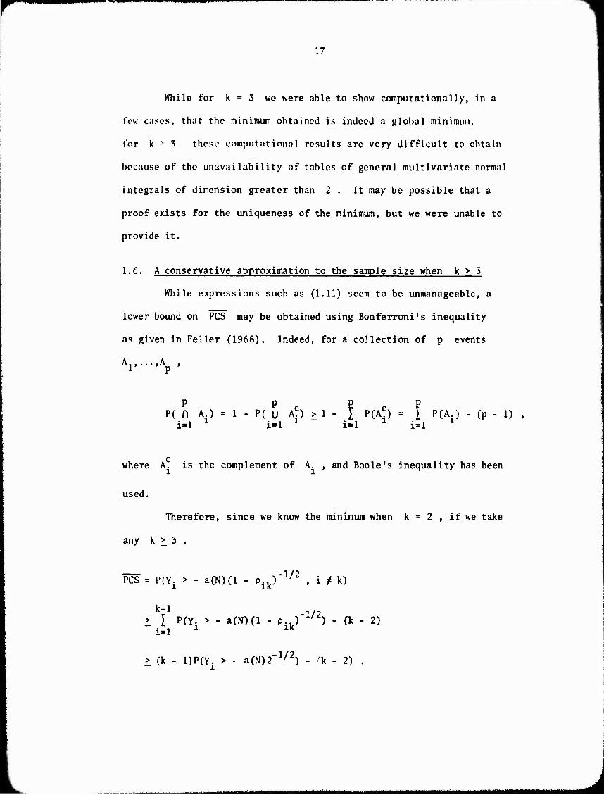
1.6. A conservative approximation to the sample size when k >. 5

While expressions such as (1.11) seem to be unmanageable, a

lower bound on PCS may be obtained using Bonferroni's inequality

as given in Feller (1968). Indeed, for a collection of p events

A^-.-.Ap ,

p PEP P( 0 A ) = 1 - P( U A^) > 1 - I ?(AC) = I P(A ) - (p - l) ,

i=l i=l i=l i=l

Q where A. is the complement of A. , and Boole's inequality has been

used.

Therefore, since we know the minimum when k = 2 , if we take

any k ^ 3 ,

PCS = PfYj > - a(N)(l - Pikr1/2 , i / k)

k-1 1/9 1 I P(Y. > - a(N)(l - P..) ' ) - (k - 2)

i=l 1 1K

> (k - l)P(Yi > - a(N)2"1/2) - 'k - 2) .

■■ ■-■- ■ III InillMIII« I ' ■— '- ■■- .-...»:. —..■.■-.J.-,^^..».-J—^.^ ...^■„^^»»Jû_M-aiMtMM»ÎMt««MUl^^M«-»J»Mll«ia

mmmmmmmmm^**

18

Sn tjnt; the right-hand side equal to P* , one may easily

solve for :' using tables of the standard univariate normal distri-

bution.

It is also possible to use the results we have for k = 3 ,

possibly in conjunction with results for k = 2 , to obtain a Bonfer-

roni approximation. For example, suppose that k = 5 . Then,

PCS iPlYj > - a(N)(l-p15)'1/2 . Y2 > - a(N)(l-p25r

1/2)

+ PCY3 > - a(N)(l-p35)"1/2 . Y4 > - a(N)(l-p45)"

1/2) - 1

> 2P(Yi > - .5(1 - T)1/2(1 + T)"1/2 . i = 1,2) - 1 .

Setting the right-hand side equal to P* , with the aid

of Table 1.1, one determines N .

1.7. A sequential procedure

Paulson (1964) devised a sequential procedure for the problem

of selecting the normal population with the largest population mean,

when the variances are known and equal. This procedure is fully

sequential and truncated, in the sense that populations are eliminated

as sampling proceeds and there is a predetermined upper bound on the

total number of stages. In this section we show how Paulson's

procedure can be slightly modified to handle the problem of correlated

variates, when the variances are known, but not necessarily equal.

Since the proof that this procedure guarantees the PCS over the

preference region parallels Paulson's proof, we prove only what is

strictly necessary and refer the reader to Paulson's paper for the

■.^.■w

19

remaining details. In what follows, we will use, as far as possible,

Paulson's notation.

Let (X. ,...,X. ) s = 1,2,,.. be a sequence of independent

vectors each with a multivariate normal distribution with unknown

population means (M.,...,^.) , known population variances

2 2 (o ,...,a ) , and unknown population correlations p.. = corr(X. ,X. ) . llv XT 15jS

Our objective is to select, with probability at least P* , the com-

ponent with the largest mean, whenever Wr^-i - Pr. , i ^ <5* > 0 .

Let 0 < X < 6* be an arbitrary fixed number, and set

—2 2 o = max (a. + a.) . Next define,

i^j 1 J

ax = [ä2/2(6* - X)] log ((k - !)/(! - P*)) ,

and W. = the largest integer less than a./X . (Note: Our definition

of a is different from Paulson's.) Then Paulson describes his

Rule P.: "At the first stage of the experiment we take one

observation from each variate , obtaining ... (X..,X-,,• .. ,X. .) .

Then we eliminate from further consideration any variate j for

which

X.j < max {X11,X21,...,Xkl} - ax + X

If all but one variate are eliminated after the first stage of the

experiment, we stop the experiment and select the remaining variate

as the best one. Otherwise we go on to the second stage of the

experiment and take one observation on each variate not eliminated

r , ^- '" •'"'

I I 'II

20

after the first stage. Proceeding by induction, at the rth stage

of the experiment (r = 2,3,...,W ) we take one observation on

each variate not eliminated after the (r - 1) stage, and then

eliminate any remaining variate j for which

r r £ X. < max { y X } - a. + rA ,

where the max is taken over all variates left after the (r - 1)

stage. If only one variate is left after the rth stage, the experi-

ment is terminated and the remaining variate is selected, otherwise

we go on to the (r + 1) stage. If more than one variate remains

after the W. stage, the experiment is terminated at the (W. + 1)

stage by selecting the remaining variate for which the sum of the

(W. + 1) observations is a maximum."

Lemma 1.8. For each 0 < X < 6* , Rule P, guarantees the probability

requirement

inf PCVy' R5 lp*

where

fi = {(M.R)|Wrkl - ^n-n 1 ö* . R is a correlation matrix.}

Proof. It follows from the lines at the bottom of p. 176 of Paulson's

paper that in {} ,

k-1 K-i n n P(incorrect selection) < 1 p{ 1 \ * 1 * -a.+nX for some n < »)

v=l s»l1cs s=l vs A

uliiilir.i.irirr ir i ■innillTM i<ilHlllMa^^

21

and,

P( I t\s-\s*V > ax for some n < » )

2(VVX)ax -2{6*-X)a, 1 exp 2 2 ~ - exp I-! fL_

a +0,-20 a p , o +0-2(7 o. p . vk vk^k vk vkvk

■2{6*-A)a1

1 exp 2(6*-A)a

(a +0i,) v v k

— 1 exp Ö2

X 1-P* " 1-k

Therefore,

P(incorrect solution) £ 1 - P* and PCS >_ P* .

In the first inequality above we have used the fact that

the equation

t(Xvs-\s+A) t2 0 = Ee ^ J = exp{t(Mv-Mk+X) + T C^/^ô^p^)}

has the unique nonzero root

tn = - 2(u -p,+X)/(o2+a12-2a a, p , )

0 ' v k -" ^ v k v k vk^ QED

■ - i — --

mmm

CHAFTKR 2

SELECTION OF THE VARIATE WITH THE SMALLEST POPULATION VARIANCE

FROM A SINGLE MULTIVARIATE NORMAL POPULATION

2.0. Introduction

The problem studied in the present chapter was motivated by

the problem posed in Section 4.3 of Chapter 4. The asymptotic solution

provided by Theorem 2.3 will be crucial to the developments of

Chapters 3 and 4.

In this chapter we study single-stage procedures for selecting

the variate with the smallest population variance from a single

k-variate normal distribution. We formulate the general problem in

Section 2.1. In Section 2.2 we obtain exact small-sample results

for k = 2 . However, when k > 2 , it does not seem possible to

extend the analysis for k = 2 , as we point out in Section 2.5. In

Section 2.4 we show how a conservative approxima ion to the single-

stage sample size can be obtained. In Section 2.5 we develop a large-

sample solution for the general case k j> 3 . for k >. 3 , and

arbitrary correlation matrix, it turns out (perhaps surprisingly)

that the least favorable configuration of the correlation matrix

depends on N , the single-stage sample size, in a very complicated

way. This is reminiscent of the results of Chapter 1. The large-

sample results of the present chapter are special cases of the results

of Section 3.1 of Chapter 3. These large-sample results, although

stated in a normal framework, are valid for large classes of multi-

variate distributions, for which Lemma 2.8 is also true.

22

— .^^_^^M^.^_^^^^^,^M,M^-M^,,M,,«,»MM^

mmmm

21

2.1. Formulation of the problem

We consider a k-variate normal population with population

2 2 means (vi.,...,p.) , population variances (a ,...,a.) and population

correlations p.. (1 < i < i •■ k) . We denote the covariance matrix ij — J — '

by E={a..}=aRcr, where 5 = diagCa.,... ,a, ) and R = {p..} IJ 1 K Ij

2 are k >< k matrices. Therefore, a.. = a. are the variances. Let

ii i

2 2 2 the ranked values of the a. be ori, < ... < ari , . The expen- i [1] - - [k]

menter does not have any prior knowledge concerning the values of the

parameters of this multivariate normal population, or of the pairing

2 of the o with the variates.

[i]


The experimenter's goal is to select the variate associated

2 with a,., , the smallest population variance. Two constants

{6*,P*}, e*>l, l/k<P*<l, are specified prior to experimen-

tation. We denote the probability of a correct selection when decision

procedure R is used by PCS«(a,R) , and restrict consideration to

decision procedures which guarantee the probability requirement:

(2.1)

where

inf PCSR(a,R) >_ P*

~ 2 2 ß = ((5,R)|a,-, >^ 0*arii ' R a correlation matrix}

Bechhofer and Sobel (1954) proposed the following decision

MHMHHMMMBi

24

procedure, when considering this problem for the case R = I. . A

sample of N independent vector observations, (X. ,...,)L )

(1 £ a _< N) , is taken and one computes.

N n lii = ^ CXia -*0' where Xi = I hJH (1 1 i 1 k)

a=l '" QI=1

Rule BS: Assert that the component associated with 2

a, , - min{a ., ... ,a,, } has population variance a,., .

Our task is to determine the smallest sample size N necessary

to guarantee the probability requirement (2.1) when Rule BS is used and

R is an unknown correlation matrix.

Subset formulation

In certain situations, the experimenter may be interested in

the selection of a subset of variates, which includes the variate with

the smallest variance. A constant {P*} , 1/k < P* < 1 , is specified

prior to experimentation. Letting PCS-(a,R) be defined as above,

we restrict consideration to decision procedures which guarantee the

probability requirement:

(2.2) inf PCSp(a,R) > P* cf,R ^ -

The following decision procedure, proposed by Gupta and Sobel

(1954), when considering this problem for the case R = I, , will

be used:

Rule GS: Include the variate associated with a.. in the selected ii

subset if a.. <_ d**!.,,, , where d* > 1 is a specified constant.

2b

Our objective is to find the smallest sample size N which

will guarantee the probability requirement (2,2) when Rule GS is

employed and R is an unknown correlation matrix.

Throughout this chapter, we assume, without loss of gene-

2 2 rality, that a < o. Cj ^ 1) . No consideration will be given

to the population means, since their configuration is irrelevant for

our purposes.

2.2. Case k - 2

In this section we consider the case k = 2 , i.e., the parent

population is bivariate normal. Writing p _ = p and

I = (a J) , we have

Lemma 2.1. The joint p.d.f. of a and a is

. n . n . ii }^ JV1 ii

" 2 O") % exp(-a V/2) (2.3) p (y^y,) = I c (P) n i i

aira22 1 ^ j=0 J i=l H+j 2- r(| + j)

y. > o ,

where

J r(|) j! j=o J

Proof. Let A = (a. .) , a.. = T (X. - X.)(X. - X.) . Then A

has a Wishart density. Make the transformation of variables a1 = a. ,

mmmm mrwmm^^mmir^^^m.Mi 11

a22 = a22 ' rl2 = ai2ail a22 ' and then obtain (2-3) as the

marginal p.d.f. of (aâ ) . Note that the joint p.d.f. of

âil,a22'' is a wei8htecl sum of products of gamma densities. QED

Lemma 2.2. Let

v = a22ö a22all

a11a11 aiia22

Then the p.d.f. of v is

(2.4) J4-I

Pv(^ = I c.(p) r(2^n) 2 zJ 2 \l + z)-^+2J)

j*0 J (r(j+n/2))^

I c (p)f (z) , z > 0 j=0 J J

Proof. In (2.3) make the transformation

a22ail a = a.. , v 11 11 a,,o 11 22

then integrate out y , obtaining (2.4) as a final result. The p.d.f.

of v is a weighted sum of central F densities. QED

Lemma 2.3. Define

b = r f.(z)dz . 3 i/e* ^

Then b < b, < b„ < o — 1 — 2 —

Proof. For j > 1 ,

in TriririMir.ilri.ir rii.iiii.il I ' r I ,tMillMtM|||tM|M|M||i||||||M<^^

(2.5) b. - b.., ^^ r ^'\i. 2r(^) n.

(r(j+-2-)ri/0*

dz

LlnilL-ü. r >J-2 (1 + z)-^2j.2)d7

(f(^j-ij)2 i/o*

It is easy to show that, ^f we integrate by parts the first

integral in (2,5), and then twice integrate oy parts the second

integral in (2.5), we obtain,

b. - b. , J J-l

j*?-l

QED

If the experimenter uses Rule BS, we obtain,

Theorem 2.1. The least favorable configuration of the relevant parameters

2 2 is a[2] = 9*a[1] , p = 0 , yielding.

(2.6) inf PCS(5,P) = p -^ z2'\l + z)-ndz .

ü i/e* (r(|j^

Proof. If p = ±1 , we have PCS(a,p) = 1 . Indeed, in this case,

X2a " ^2 = b(Xla " V a-e- H 1 ct < N) ,

where b = oa /a . Hence,

22 I (X a=l 2a

7 ^2 u2 X0) = b a 11 Taii a-e-

resulting in

— - -■■■^■■~ B

28

PCS(ä,p) = P(an <_ a22) = P(a^ 1 a^) = 1

2 2 For other values of p , and a > ö*a ,

PCS(5,p) = P(a11 < a22) = P(v > c^/a2) >_ P(v > 1/9*)

= I c (p)b

Since b- = inf b. , and c„(0) = 1 , it follows that 0 jô J 0

inf rCS(0,p) = hn . QED

Bechhofer and Sobel (1954) provide a table of values of the

integral on the right-hand side of (2.6). For 9* and P* specified,

the experimenter uses the table to determine N = n + 1 .

Lemma 2.4. Consider a loss function L. (a,p) = loss when component

i is selected and (a,p) are the parameters, such that,

2 2 (i) L. (a,p) <^L.(a,p) when a. > 7. ;

2 2 2 2 (ii) 0 1 Lâ.p) = L^.Cw.p) , where ir^.ap = (iraîra ) is any

2 2 permutation of ia.,a ) .

Then Rule BS is minimax and admissible, uniformly minimizing

the risk function among all invariant (under permutations of compo-

nents) procedures.

Proof. Since c.(p) >. 0 for all p , and since the gamma densities

appearing in (2.3) have monotone likelihood ratio, invoking a result

of Eaton (1967a) (a generalization of a theorem of Bahadur and Good-

man (1952)), the conclusion follows at once. QED

„ — 1 1 1 1 ilmlr -' j^^njgnggmiigniK

29

If the experimenter uses Rule GS, we have,

Theorem 2.2. The least favorable configuration of the relevant

parameters is

2 2 aril = ar2l ' p = 0 ' yielding,

2-4 (2.7) inf PCS(5,p) = f* ^"J 2

2 (1 + z)'nd2 1/d* (r(|))^

Proof. The proof parallels that of Theorem 2,1.

Lemma 2.5. If S denotes the size of the selected subset when

Rule GS is employed, then

(a) E(S|5.p) = P(v > jf^-) + P(v > ^-) 1 a 22 11

where v and v are both distributed as in (2.4).

(b) sup E(S|a,p) = 2 , when o, = 09 . P = 1 .

Proof. The result follows easily from previous developments.

2.3. Case k >. 3 .

In this section we develop some preliminary results for the

case k >^ 3 , and outline some o; the difficulties encountered. We

have not been able to obtain definitive general small-sample results

when k ^ 3 . Unfortunately, the method employed for k = 2 in

Section 2.2 fails here. In particular, it is easy to develop similar

results to those given as Lemmas 2.1 and 2.2, but there is very strong

evidence that the least favorable configuration of R depends on N

•—■—"-■ ^MMMMHHMMMMHMIIIHMMai

30

and e*(or d*). This will be seen in Section 2.5, where we develop

complete asymptotic (N + ^ results.

If Rule BS is used, without loss of generality, we assume

2 2 a ■ 1 , a. = 6* , j / 1 , since this is a least favorable con-

figuration of the variances. Indeed, in n , we have,

PCS = Pian < a..,j^l) = P(o2lX

2n(l) < aÛ))

iP(X^(l) < e*x^ü),jî)

where x'(j) (1 1 j < k) are the diagonal elements of a Wishart n

matrix with mean nR .

We define

R =

1 lu an A12

.^l V , A =

A21 '22.

N = I

a=l (xa-x)cxa-x)

where Z . and A are (k-1) x (k-1) symmetric positive definite

matrices. Then, the following lemma is stated in a slightly dif-

ferent form in Johnson and Kotz (1972), p. 223. It provides a con-

venient representation for the distribution function of the diagonal

elements of A,

Lemma 2.6. The conditional distribution of a. given A is

noncentral x_ » with noncentrality parameter

lUl22k22l22hl

2eni-E12^r21)

■.«■■ ■ i»'w^^^mmmnmmrmm^

31

In other woras.

Pa lA (') = ^ ^TT P 2 (')

2fj

If p. (•) denotes the density of the Wishart matrix A22

A,,,, , we have

(2.8) PCS = / P(a < a j/l|A )p (W)dW W>0 J] 22

mm a. .

= / PA (W) I e X 1"E12J:222:21

A *- k' W>0 22 kxO 0

p (u)du dW ,

where W > 0 means W symmecric positive definite.

Using (2.8), a tedious but straightforward computation shows

that

3PCS = 0 (i M). at R = I, 3p. . " ^ r •"• "- ^

One might conjecture, in view of this last result, and the results

of the previous section, that R = Ir. is a least favorable configura-

tion of R . However, we dot believe this to be the case for k > 2 .

In fact, we shall prove in Section 2.5, using asymptotic (N ■*• <*>) distri-

bution theory, that R = Ik can be a saddle-point of the PCS . It

1/2 approaches a global minimum when ceit(n) = (l/2)n log 0* ->■ ~ . When the

. . .1 . I, i i i Bfi^BB^BBtmmmmammmmmmmmmiBtmmtmmmammmmmmmmmmmmmmmmmmmmmm

32

experimenter knows that the off-diagonal elements of R are equal,

then we show in Section 2.5, using asymptotic theory, that R = Iv

is a least favorable configuration, which does not depend on N

and 9* . In other words, we are facing a situation similar to the

one encountered in Chapter 1, where the least favorable configuration

varies with the sample size.

The same remarks are valid when Rule GS is used.

2.4. A conservative approximation to the sample size

In view of the difficulty of determining a least favorable

configuration of R for k >. 3 , the following Bonferroni approxi-

mation (cf. Section 1.6 of Chapter 1) can be used to determine a value

of N , which will be larger than the minimum N required to guarantee

the probability requirement.

Lemma 2.7. If Rule BS is used.

5-1 (2.9) inf PCS(0,R) > (k-1) r ^ j z2 (l+z)"ndz - (k - 2) .

n i/e* crc|)r

Hence Bechhofer and Sobel's (1954) table may be used to

determine a conservative value of N « n + 1 .

If Rul>; GS is used, a similar approximation is available,

replacing 6* by d in (2.9).

2.5. Large-sample theory

In this section we develop a large-sample theory for the

problems considered in Section 2.1. One of the results obtained

(Theorem 2.3) will be used in the next two chapters as an important

m^Bftmm

~mmmmmm^^^^^^^~~~~'^^*^—ma^m^*'^~~** ■■ ■■ ■-— -■■"

33

tool for obtaining large-sample results. We start with a version of

the Central Limit Theorem, stated and proved in Anderson (1958), p. 75,

Lemma 2.8. Let Xa , a = 1,2,..., be a sequence of independent

k-dimensional normal vectors, each with mean vector u and covariance

matrix Z = (o..) . Let

i N _ _ B(n) = (b (n)) = n2{(l/n) £ (Xa - y^ - y1 - z] ,

a=l

where

N Xx ,= I X /N , n = N - 1 .

ci=l

Then the asymptotic (N •*■ «.) distribution (a.d.) of B(n)

if multivariate normal, with zero means, and covariances

E{b. .(n) • b. „(n)} = o.-O., + a. a, ij k£. ik j£ li 3k

Another tool that will be used extensively, is given below as

a lemma, the proof of which may be found, for example, in Rao (1968),

Chapter 6.

Lemma 2.9. Let (Y ,...,Y. ) , n = 1,2,... , be a sequence of not

necessarily independent vector variates, such that.

n1/2rv fl0 Y fl0-» n (Yln - \.--'.\n - ek)

has multivariate normal asymptotic distribution with zero means and

covariance matrix I . Let gj.-.-.g be real functions defined on

i T Bimn - ■- --■-:'- -- ■"—-—— — ^.-^ - .-.-^..^ ^^^^^ .w^: ^„^^„»aaa^M».^.

■ )i"'"'' mm um wmmm^mmmmmmw^^^^ ■■■ > "^ -••l

34

E^ , the k dimensional Euclidean space, which are differentiable in

a neighborhood of 0 = (0 ,...,0 ) , Then the a.d. of

"^^^În-'-^kn3 " S^9?«---'9^) (1 1 j ir) , is multivariate

normal, with zero means, and covariance matrix,

^(6°) ^ (V^ZVg.) .

whore

3g. 9g

1 k 'J (1 1 j ir) ,

if T.(Q'J) is nonsingular.

We shall use the notation introduced in Section 2.1, and assume,

2 2 without loss of generality, that a < a. (j ^ 1) .

Lemma 2.10. The a.d. of

(2.10) Y. = J/2fl°g(a11/a 3-log(aâ^ n u—T-rrr1 i 2(1 -P]/^

a ^ i) .

is standard multivariate normal, with correlations.

corrCY-.Tj) E Y..

,222

2(1-P12i)

1/2(1-Pjj)1/2

(i * j)

Proof. From Lemma 2.8, the a.d. of

n1/2(aii/n - o*) (1 < i < k) ,

rMM^MMMMMm

35

is multivariate normal with zero means, variances equal to 2o. ,

;iiul covarianccs Zo". . Therefore, using a variance stabilizing

transformation (cf. Bartlctt and Kendall (1946) and Lemma 2.91, we

have that

n (log(a../n) - log a.) (1 < i ^ k) ,

has a multivariate normal a.d. with zero means, variances equal to 2 ,

2 and covariances equal to 2p.. . Finally, (2.10) is obtained using

Lemma 2.9 once again. QED

The proof of the above lemma is essentially contained in

Ramberg (1969). Note that (2.10) resembles the distributions of the

previous chapter (cf. Lemma 1.1).

Let PCS denote probability of a correct selection when

an asymptotic (N ->■ oo) distribution function is used. The following

is an important result for our purposes.

Theorem 2.3. If the experimenter uses Rule BS, the asymptotic

(N ■> <*>) least favorable configuration of the relevant parameters is

6*0[U = 0[2] •• = "[k] • Pij = 0 (i ^ »

Therefore,

(2.11) inf PCS (a.R) = ^(Y. <_ n1/2(l/2) log 9* , j / 1) ,

where the (Y.J ^ 1) are distributed as in (2.10) with

Y.j = 1/2 (i / j) .

-'■-'■"■ -■■- >"--"' MMMtMküiHiaMi mmm

3b

Proof. In Ü .if o^ < a^ (j j« 1) ,

l/^,^. 2^2, n'^logCaVaf) l'CS(a.R) = P(a < a j ^ D = p(Y < * , j^l)

> I'CYj < n1/-,(l/2)(Joi. 0*H1 - pp'1/2 , j ^ 1)

*(Y..)(Cü*(n)fl " Pi2rl/2---'co*(n)(1 " Plkrl/2)

wnero,

and

c.Jn) = n1/2(l/2)log 0* ,

CT^) - <trY..)(c2Cn)'--"clc(n))

c.(n)

f(Yi.)^2'

ceJn)(l - P^)"172 (j ^ 1)

.,yk)dy2...dyk .

and f(Y..)(y2'---'yk) is the P-d'f- of the iY j / 1} . Since,

JJ- = 2p,.fl JJ-a 0 8p kÄ

ki an2 8PkÄ

if all p . = 0 , it follows that the correlation matrix R = I. is a k* K

stationary point of $, ^ . We must show that it is a point of

global minimum as cQi(n) -> " .

-- ■ —*■-

wmmm

37

First assume p ^ 1 (j ^ 1) . We will prove that

3^ (Yii)

~ J > 0 C£,m > I) . 9p im

Without loss of generality, consider 1=2, m = 3

(2.12) V.) 8Y

Mi- 23 rC4(n) r

Ck(n^ f f, r , 2 2

aP23 3p23 -CO _oo îj) 2 -3V"^'4' ,yk)dy4...dyk

>0

since

3Y 23

(1/2)(1 - 3p

^■1/2» ^3'-1/2 > o

23

Next, we show that, as c *(n) ->■ » ,

a* (2.13) -^— > 0 (P J« 1)

3p IP

Without loss of generality, take p = 2 . Since p . appears

in the expressions of y ,. .. ,y , , we have

...,....■. -■...-. .— - ^ -■■ . ■-J- ■ ■-"■■ft ■.--^-■.-^■--—^--^ |aa^MM^(i||MjaMa)M|||gyBjg,M|âMM|M||<|^^

«^mnrnap^^ •^mi^^^mw-

38

(2.14) —J^-- I 3p 12 j=3 '2;

p;2 fixed 9p12 3p?2 Y.. fixed

j»3 ap12 -«

3c, (n) ^c^n) .c,(n)

tY..)^""^ j-l' j

yj+1.....yk)dyv..dyk

— /j .../^ fCYi.)(C2(nj'y3'---'yk)dy3---dyk

3p -* -*

k 9Y, ac2(n)

7 . 2 "2j ' 2 ^2 J=3 3p12 9p 12 Q. •

where

9c2(n)

3p c0*(n)(l/2)(l - Pi2r

V2 ^ » as c0Jn) ^ » ; 12

CIS) 3Y9.

3p 12 4(l4)1/2(l-p22)3/2 12j

TTTTfT, 2 ,3/2 4(1^^) (1-P12)

Since M2. > 0 (j >, 3) and Q2 > 0 , we only have to consider

9Y2i situations where —f- < 0 for some j . Suppose, for instance, 3p12

3Y that 23

3p j- < 0 . This is equivalent to X < o . We will show that

12

Q2 - M23 > 0 , which proves (2.13), in view of (2.15).

A straightforward computation leads to

- — ^ 1^— lim^mmmmitimmmilimtigmm^^

■•"^^■w^^w™»"««" "

39

(>4(n)"Y24C2(n) C,k(n)_YPkC7(n)

Q -M = f(c-(n)) /4 24 2 ... /k 2k 2

cr3(n)"Y^3c^n)

i / '' fCz^.---.zk)dz3-f(c3(n)-Y23c2(n),z4,.. .,zk) }

4 k

where

1 C2(n)

f(C2(n)) = ryy exp{ r— } {2-n) ' l

and f is the density of a multivariate normal distribution with

zero means and covariance matrix which depends only on the Y-• (i ^ j)

Since * < 0 , we have

ce*(n)(-X123) c3(n1 - Y23c2(n) =—2 1/2 2 - - as V(n) -» .

2(l-p13) (l-p12)

showing that Q2 " M23 > 0 • This' in turn' implies (2.13)

- ■■'■—-■—"-—•'—^■- «MMMMMiMMMaMaHMIiHIIMlliaHBHHHHMHMMHMHaHHMHHIHaMaailH

PWWwnwwpPW>»WPwwiWFW»wpw

40

Equations (2.12) and (2.13) imply that

*(Yij)(c2Cn) ck(n)) ^*(i/2)(ce*(n)'---'ce*Cn))

This last lower bound is achieved when P.. = 0 (i / i) .

2 proving (2.11) when p . ?* 1 (j j< 1) .

2 Let J = U,,...,jj} , 1 £ J . Assume that p . = 1 , j € J

Using an argument similar to the one employed in the proof of Theorem

2.1, we have,

all = (0l/öj)aJ3 a,e" (j € J)

2 2 Therefore, for such an R , if a < a. (j ^ 1) ,

PCS = P( H (a <a )) = P( n (aJ<oJ) , fl (a. <a..)) j>l 11 JJ J€J 1 J j^J 11 "

Since, for any R ,

P( n (a.. < a )) >.P(n (a < a )) j^J 11 JJ j>l 11 "

_~~— mi-ini i Mi M^MMBMMMMMMMâBMMMMBaaMaaMgMaMMg^^MâiâMa^gaaMMMaiâaaaBMMBMMMlMBM

mmm^mmi*'"!'*'

41

it is seen that p = 1 , j £ J does not lead to the infimum. QED

Theorem 2.4. If the experimenter uses Rule GS, the asymptotic

(N -*■ a') least favorable configuration of the relevant parameters is

'k ' Pi:j = 0 (i / j)

Therefore,

(2.16) inf PCS (5,R) = P(Y < n1/2(l/2) log d* , j M) , ■» J

where the {Y. , j /I} are as in Theorem 2.3.

Proof. The proof is similar to the proof of Theorem 2.3.

Lemma 2.11. If S denotes the size of the selected subset when

Rule (IS is employed, wc have asymptotically (N -^ «O ,

i 1/2 2 .-l/21„„f^ 2. 2, (a) l:a(S|5.R) = I P(Y <n1//{l/2)(l-p^ )"1/Zlog(d*a'/ap , i / j)

where the (Y. , j ^ i} are distributed as in (2.10) with i in

place of 1 .

(b) sup E (S|a,R) = k when a2 = a2 (i ^ j) , R a i j

1 ... 1

1 ... 1

Proof. Consequence of previous developments.

Theorem 2.5. Suppose that p. . = p (i ^ j) , where p is unknown,

Then,

(a) If Rule BS is used, an asymptotic (N + «) least favorable

—~— " ■ ' ~~--~~-~~~-~~~~-~~~~-~-~*~»'m~m***-~m

42

configuration of the relevant parameters is

^[l] =a[2] = '•• =a[k] ' p = 0 '

(2.11) being pertinent;

(b) If Rule GS is used, an asymptotic (N ->. ») least favorable

configuration of the relevant parameters is

2 2 öj = ... =ak , p = 0 ,

(2.16) being true.

Proof. This follows directly from Lemma 2.10, without the need for

further arguments.

There is evidence that the approximation used in Lemma 2.10

is very good, even for small values of N . The reader may consult

Bechhofer and Sobel's (1954) tables where some comparisons are given.

Hence, we would conjecture that Theorem 2.5 provides an excellent

approximation to N , even for relatively small values of N . As

for Theorems 2.3 and 2.4, we have used the fact that N is large

in a stronger manner, but still it is expected that moderate values of

N would provide a very good approximation to the small sample

results. We would expect that the approximation will be an excellent

one if P* and 6* are close to unity. Values of N may be deter-

mined using formulae (2.11) and (2.16) in conjunction with the tables

of Gupta (1963) or Milton (1963).

We next explore the behavior of *, -.in the vicinity of (Y.j)

R = I. . It is easy to compute, from (2.12) and (2.14), that at

R=Ik.

- ■ -■ •"—fM—nafrgygngm^!^

43

:)(, im

> 0 (£,ni > 1)

IM,

"V,, -h R=I.

4 J ••• i f(i/2)(ce*(n)'ce*(n)'y4"--' yk)dy4...dyk

cfl*(

n) c.0*(n) c0 rn) 9* rQ* rQ* ■

' •■• f fr^/7^tC(i*M^y^.^^^>yJdyT■^dy (1/2)^9 kJ '5'

Therefore,

(j > 1)

3* (V^

<

0 if ceJn) = 0 ,

R=I.

and > 0 if r (n) ■+

In other words, if c (n) is sma.1.! enough, *f . has a saddle- lYijJ

point at R = I, , while as c (n) increases it will have a local

minimum there, and eventually a global minimum.

Finally, we show that PCS can be less than 1/k , as was

also the case in Chapter 1. Note that 1/k is the lowest possible

value for the PCS when R = I. . Take k = 2 , k

2 2 P12 = P13 = 1/2 ' P23 = 0 " Then' Y23 = 0 and

PCS c (n) c (n)

/ / Wy^y^y-A,a 1/4 < 1/3 -00 _00 (0)^2^3ÛJf2u/3

if ce*(

n) = 0

. .

mmmmmmmmmmm

CHAPTER 3

SELECTION OF A SUBCLASS OF VARIATES WITH THE SMALLEST POPULATION

GENERALIZED VARIANCE FROM A SINGLE MULTIVARIATE NORMAL

POPULATION (ASYMPTOTIC THEORY)

3.0, Introduction

In this chapter we study selection procedures in terms of

population generalized variances associated with subclasses of variates

from a single multivariate normal population. In Section 3.1 we

consider disjoint subclasses and the results obtained are extensions

of the results of Section 2.5 of Chapter 2. In Section 3.2 we consider

intersecting subclasses. Many other selection problems in terms of

generalized variances may be treated using the ideas of the present

chapter. We decided to restrict consideration to these two particular

problems, since they illustrate well the methods we propose. For

instance, it is easy to extend these results to selection problems

involving subclasses of different sizes. Throughout the entire

chapter, the theory developed is asymptotic (large-samp1e), and could

he stated in a more general framework than normality.

3.1. Selecting the smallest population generalized variance (disjoint

subclasses) .

Consider a kp-variate normal population, with unknown popu-

lation mean vector and unknown population covariance matrix.

44

«Ml^MMMiaM ^^MlMMMMMMMMMMiBHH

r*—~*^m*m

£, E..

T. 7, 21 2

[?:kl };k2

Ik

■2k

where 5". U 1 j £ k) arc p x p .symmetric positive definite

matrices. The quantity det £. is referred to as the population

generalized variance associated with the ith subclass of variates

fl < i -^ k) . Let det 5:f]1 < ... < det T. r. , be the ranked values

of the det I. (1 <^ i < k) . It is assumed that no prior knowledge

exists concerning the values of det Z. H 1 j £ k) , or of the

pairing of det Z... with the subclasses of variates.

Indiffcrcncc-zone formulation

The experimenter's goal is to select the subclass of variates

associated with det Z , . He specifies {9*,P*} , 6* > 1 ,

1/k < 1'* < 1 , prior to the start of experimentation. If PCS (E)

denotes the probability of a correct selection when decision procedure

R is employed, we restrict consideration to procedures R which

satisfy the probability requirement:

inf PCS.m > P* , Q K -

where

fl|det £. > • det E , J ? [1])

In this chapter we propose "natural" single-stage selection

■Ml

mmmmmm

■16

procedures, which associate sample quantities with the corresponding

population parameters.

A sample of N independent kp-vector observations,

X = (X ,...,X. ) (11« 5 N) , is taken, and the sufficient

_ N N statistics (^.S) , XN = £ Xa/N , S = I <i*a - ^ (\ - \) /n ,-

a=l a=l

n = N - 1 , are obtained. Let S be partitioned according to £ ,

in such a way that S. corresponds to T.. (1 <^ j £ k) , and

S. . to E. . (i ^ j) . For this indifference-zone goal, we adopt

the following decision rule:

Rule R„M : Assert that the subclass associated with UV 1

dot S, , s min det S. , has the smallest population generalized

variance, det E r . .

Our objective is to determine the smallest sample size N

such that Rrv will guarantee the probability requirement.

When £..=£* (i j^ j) , R v, is minimax, and also has

uniformly smallest risk for a class of natural (invariant) decision

procedures and loss functions (cf. Eaton (1967b)).

Subset formulation

If the experimenter wishes to select a subset of subclasses

containing the subclass associated with det E. , , he specified

{P*} , 1/k < P* < 1 , prior to the start of experimentation. If

PCSp(I) has the same meaning as above, we restrict consideration

MMHMUtaiaUliMiartMM iiiiiiinr iti<MtMM|igMM|a||g

mmmwM

47

to decision procedures R which satisfy the probability requirement:

inf PCS (>:) > I'*

goa 1:

We propose the following decision procedure for this subset

Rule RpV-,: Include the subclass of variates associated with

S. in the selected subset if det S, < d* det S,,, , where d* > 1

is a specified constant.

Our objective is to find the smallest sample size N which

will guarantee the probability requirement when R„.,0 is employed.

Gnanadesikan and Gupta (1970) studied R ™.- for the case

where 3^. . = 0 (i ^ i) . ij J

We disregard the population means in what follows, since they

.ire irrelevant in our problems. We assume, without loss of generality,

that det E, < det Z. (j ^ 1) ,

The following linearization result, proved in Siotani and

llayakawa (1964), and which goes back to Olkin and Siotani (1964),

will be used extensively in this and the following chapter.

Lemma 3.1. Let Li be as above, Z = (a ) , and f. (S) , j € J ,

.1 a finite set, be real valued functions of S , not algebraically

dependent, having first and second derivatives in a neighborhood of

Z (in the topology inherited from E ° ^ -" ^ ) . Then, the a.d. of

n1/2(f.(S) - f.m) (j 6 J)

i i - ^M—w-iBr ■IMMUHM

48

is multivariate normal with zero means, variances equal to

2 2 2(f.(E)) tr 0.(j:)E) Cj € J) . and covariances equal to

2fj(J:)fi(J:) tr (fjCJ:)E<J.i(E)Z (ij € J) , where

aa3 = (1/2^1 + V^

aß 1 if a =

aß

0 if a ^


1/2 n (det S - det ^.....det S, - det E, ) 1 1 k k'

is multivariate normal, with zero means, variances equal to

2p(det E.) , and covariances 2 det I. det £. tr E. I..E. E.. .

Proof. This lemma is a consequence of Lemma 3.1. Using the notation

peculiar to that lemma, let f.(E) = det E. . Then, it is known

(cf. Anderson (1958), p. 347) that,

^(E) =

,-1 1

0 0

LO 0

0 0

0

OJ

*2(Z)

0 0 cf

0 ^

0

0 0 o_

Noticing that

-- -

49

trCÔOSr = tr

tr ^^1)1^(1)1 = tr

0 0 ..

IP 0 ..

1 Z"1! p 1 12 ••

0 0 ..

0 0

1 IK

0

0 j

0

o J

= p

0 0

2 21 p

Loo

= tr ''IWlhl '

0

E2l!:2k

0

the present lemma follows at once.

Hooper (1959) defined

QED

U .-1, 'u = (1/p) tr VVj'n

as the squared trace correlation coefficient between subclasses

2 2 i and j . If v ,...,v are the canonical correlations (cf.

Anderson (1958)) between the two subclasses, it can be shown that

^= J. v'Vp • wnich implies

0<p.. <1 .


i wo log(det S./det S.)-log(det I./del E.) (3.1) Y! = n1/2{ 1 J 2

1 i- } (j ^ 1) , J 2p1/2(l-pJ.)1/2

i^^M^^^M^MM^üMHMMMMIIMaHMI

50

is standard multivariate normal, with

corr(Yj.YJ)

! ^2 2 2 l-P^-P, .+P. .

13 2(1-0^1 2 OT^ J\l/2 » * » tl-P^)

Proof. This follows using Lemma 2.9 of Chapter 2 and Lemma 3.2 above.

Theorem 3.1. If the experimenter uses Rule R-.. , an asymptotic

(N ->- °°) least favorable configuration of the relevant parameters

is

det Z./det ll = 9* (j / 1) . Z.. = 0 (i / j)

Therefore,

(3.2) inf PCS fZ) = P(Y! < n1/2( 1/2, n a— '(Y. ln^(l/2)p^"-log 9* , j ?« 1)

where the {Y. , j ^ 1} are distributed as in (3.1) with

Yij = 1/2 (i * j) •

Proof. Using Lemma 3.3, we have for det Z . >_ 6* det Z (j ^ 1) ,

PCS (Z) = P(det S < det S. , j ^ 1) a i j

= P(Yj < n1/2(l/2)p":i/2(l-Pj.)"1/2log(det Z./det Zj) . j ^ 1)

LP(Yj < n1/2(l/2)p"1/2(l-p2.)"1/2log 9* , j ^ 1) .

We can now use Theorem 2.3 of Chapter 2, and set p.. = 0 (i ?< j) ,

to obtain a lower bound on PCS (E) . Since the parameter configuration a

det Z = 9* det Zj (j / 1) , Zi. = 0 (i / j) , leads to this

— ^MM^M^M

mmmmmm^mmmmmmmmmmmmmmmiim^^m^^mm

51

lower bound, it is a least favorable configuration.

It is easy to show that ^.. = 0 (i ^ j) , is also necessary

for an asymptotic least favorable configuration. Indeed, if

-> pT. = 0 , then £.. = 0 necessarily, from the definition of squared

trace correlation coefficient QED

Theorem 5.2. If the experimenter uses Rule R^..^, ^n asymptotic

(N -+ co) least favorable configuration of the relevant parameters

is £=...=£,, E.. = 0 (i ^ j) . Therefore,

(3.3) inf PCS fS) = PCvJ < n1/2(l/2)p"1/2log d* , j t I)

where the ^Y. , j ^ 1} are as in Theorem 3.1.

I'roof. The result follows immediately from Theorem 5.1.

I.oimiia 3.4. If S denotes the size of the selected subset of sub-

classes of variatcs when R,^,-, is employed, wo have dV z

(a) Ha(Sll) I P(Yj < n1/2(l/2)p"1/2(l-p2 )'1/2log(d*det E /det Z) , i=l ■' ■> 3

i ^ j)

where the iY. , i ^ j} are distributed as in (3,1) with 1 replaced

by i .

(b) sup E (S|2) = k which occurs when I = E a

I ... I P P

I ... I I P PJ

Proof. The result is a coneequence of previous developments.

mmmm^mtm^tmmamitm

52

It is interesting to note that Theorems 3.1 and 3.2, and Lemma

3.4 reduce to Theorems 2.3 and 2.4, and Lemma 2.11 of Chapter 2,

respectively, when p = 1 .

3,2. Selecting the smallest population generalized variance

(intersecting subclasses).

The last problem of the present chapter is a problem of

intersecting subclasses of variates, where some variates belong to

more that a single subclass. We start by proving a lemma, which will

be basic to what follows.

lomma 3.5. Let X^ = (X^.X^.X^) (1 < ct < N) , be independent

normally distributed (p.+p:,+p-)-vectors, with unknown population

means and unknown population covariance matrix

Z =

A D E

D1 B F

E1 Ft C

where A(p1 x p,) , B(p9 x p.,) and C(p7 * p,) . Define,

Xk<.= 1*\AJ ■ "ka- ^2A »I«!« • N N

:'l2 = ^ X12,a/N ' X23 = \ X23,a/N '

a=l a=l

TT .t ;12= ^ fX12,a-X12^X12.a- X12^/n' "

N - 1 ,

S23 = ^ fX23,a - V^,« - ^^

'12

A D

Du B . X 23

B F

F1 C

53

Then, the a.d. of

1/2 n (det S12 - det I , det S - det Z„)

23 2y

is multivariatc normal, with zero means, variances equal to

1 2 2(P1

+l>2)(det?;i:r and lip^p^) (detZ^) , and covariance

J(p-,+A)dct };j,2Jet 5:^ > where X ^ 0 is defined in the course of the

proof.

Proof. Using the notation of Lemma 3.1, we obtain, f.■(H = det £..

(1 < i < j 1 3) ,

*12m hi o

0 0 *25(Z}

0 0

-1 0 I.

23

The expressions for the variances follow immediately. Now we define.

n--i

hi 'l2(u)

1^1}

fA-mrVr1 -(A-DB^D^^DB"1

1 E12(M

'23

1, .-i Z23^

Vz^

Z23^

(C-F^^F)"1?^"1 (C-FVVi

In order to compute the covariance we must evaluate

— —-—-———"

tr *l2WZ*2?,(Z)l

tr 0 0 0 Ü

E12 l!

' I 0 E^ful^l 1 P1 12,-unF;

ooo o

] 0 L

= tr 1 An^ fPA o i rV^R

0 0

23

0

f A D I:

Et 2i

0 0

0

I P3 J

? = P2 + trV^(u)fF]z-l,

= p2 * tr(A-DB-1Dt)-1(E-DB-1F)(C-FtB"1F)-1(Et-FtB-1Dt)

P2 + X

Hooper (1962) defined

13.2 = VPj ,

as the squared partial trace correlation coefficient between subclasses

X and X conditional on X . If p < p (say) and

2 2 vT.^'-.v are the canonical correlations between X. and X_

1 pj 13

in the conditional distribution of X and X given X , it can

be shown that,

2 * 2 P13.2 = Jj VPl '

which implies,

1—i— 1 ■—*

mmmmmmmmmmmmmmmmmm^^mmmm ■■ mwmm*mm^^^m*îm

O*-^.!*-1 ■

Hence, 0 £ A < p . QED

We note in passing that X = o if D , E and F are zero

matrices.

In this section we consider X =» (X ,..,,X,) a k-variate

normal population, with unknown population mean vector, and unknown

population covariance matrix I. We assume k >_ 3 . Consider all

possible subclasses of specified size t (t < k) of X , whose

total number is U»( J . Let £,...,£ be the covariance matrices

(submatrices of E ) corresponding to these U subclasses, and let

det ^M-I 1 • • • 1 det Erm be the ranked values of det E. (1 1 j 1 U)

It is assumed that the experimenter has no prior knowledge concerning

the values of det E. (1 £ j £ U) , or of the pairing of the

det Er.n with the subclasses of variates. [i]


The experimenter's goal is to select a subclass of t variates

out of the k-variate population, with the smallest population genera-

lized variance, det E . . He specifies {e*,P*} , 6* > 1 ,

1/U < P* < 1 , before experimentation starts. If PCSj,(E) is as

defined in Section 3.1, we restrict consideration to decision procedures

R which guarantee the probability requirement:

inf PCS0(E) > P* o K —

^^mmm^t^^mmttlmgll0mmmmmitimtimtmtmtii

mm

56

where

ü = {j:|e*dct E^, < det I. . j / [1]} .

We propose the following decision procedure for this indif-

ference-zone formulation of the problem;

Rule R^r,: Let S be the sample covariance matrix computed

using a sample of size N from the above population, as in Section

3.1. Let S. (1 £ i £ U) be submatrices of S corresponding to

î (1 £ i £ U) . Then assert that the subclass of t variates

associated with det Sril = min det S. has the smallest population [1] j

generalized variance, det £..., .

Our task is to determine N which will guarantee the proba-

bility requirement when R™,7 is used.

Subset formulation

If the experimenter is interested in selecting a subset of

subclasses of variates, which includes the subclass associated with

det Z , he must specify {P*} , 1/U < P* < 1 , before experimen-

tation starts. If PCSp(E) has the same meaning as a'iove, we

restrict consideration to decision procedures which guarantee the

probability requirement:

inf PCSn(J:) > P* E * -

For this subset formulation, we propose.

înr iiiiinrMir m^H

WOT

57

Rule R~,,: Include the subclass associated with S. GV4 j

U 1 j 1 U) , in the selected subset of subclasses of variates if

dct S. £ d*det S,., , where d* > 1 is a specified constant.

Our task is to determine the smallest sample size N which

will guarantee the probability requirement when Rpy,, is employed.

Due to the symmetry of the present problem, we may assume,

without loss of generality, that det E. = det Iril , Moreover, we

give no consideration to population means in what follows, since

they are irrelevant for our problems.


n1/2(det S - det £,...,det S - det E )

is multivariate normal with zero means, variances equal to

2 2t(det I.) (1 < j < U) , and covariances 2(t. . + X. .)det E. det Z.

H 1 i < j £ U) , where X. . ^ 0 (defined in Lemma 3.5), and

t. . is the number of common variates of subclasses i and j

(corresponding to S. and S. ).

Proof. This result is a consequence of Lemma 3.5.

We define.

P2. = (t. . + X..)/t (i t j) , t../t < p2. < 1 .


i wo log(det S /det S.)-log(det E /det I.) (3.4) Y = n1/2{ 1 l/2

J 2 l/2 l- L- } 0 M) ,

M^ttliailBMti MHMaaaaMMkaaMMMi

58

is standard multivariate normal with

2 2 2

corr(Y .y ) sy = ll ■ ^ ^ 1 ■• 1J 2 2 1/2 2 1/2 (1 ^ J)

Proof. The result follows using Lemma 3.6 and Lemma 2.9 of the

previous chapter.

Theorem 3.3. When one employs R , an asymptotic (N -> <») lower —~——^^ (jV3

bound on the PCS, is given by:

(3.5) inf PCS fE) 1 P(Y^ < n1/2(l/2)t"1/2log 6* , j / 1) Ü a - j

where the (Y. , j ^ 1} are distributed as in (3.4) with y.. = 1/2

(i ^ j) . When t = 1 (resp. t = k - 1 ) lower bound (3.5) is

sharp, and an asymptotic least favorable configuration of the relevant

parameters is E = diag(l,e*,...,9*) (resp. Z = diag(e*,l,...,1)) .

Proof. The proof of this theorem is similar to the proof of Theorem

2.3 of the previous chapter.

Theorem 3.4. When one employs R,-,. , an asymptotic (N -> «0 lower

bound on the PCS is given by:

(3.6) inf PCS (Z) > P(Y^ 1 n1/2(l/2)t'1/2log d* , j ^ 1) Z a 3

where the (Y. , j ^ 1} are as in Theorem 3.3.

When t=l or t = k - 1 , lower bound (3.6) is sharp, and

as asymptotic least favorable configuration of the relevant parameters

is I = diag(l, ...,1) .

■-• —- - --~-^ m^^^m^^mi^^llimmmimijmi^mmm^^

59

Proof. The proof of this theorem is similar to the proof of Theorem

2.3.

Lemma 3.8. If S denotes the size of the selected subset of sub-

classes when R™,. is used, GV4

(a) Ea(S|z) k n1/2log(d*det I./det I.)

I P(Yi ^ 172 2^172 - i=l J 2ti/^l-p' )i/^

, i / j)

where the (Y. , i ^ j} are as in (3.4) with i in place of 1

(b) sup E (Slz) = k which occurs when T. = I a

1 ... 1

1 . .. 1

Proof. The result is a consequence of Lemma 3.7.

- mmilM^m -»^ ^^—miim , ^^^^^^^^^.^^^^^^^^

CHAPTER 4

SLLIiCTlON OF SUBCLASSES OF VARIATES OR OF POPULATIONS

BASED ON MEASURES OF ASSOCIATION BETWEEN TWO

SUBCLASSES OF VARIATES (ASYMPTOTIC THEORY)

■1.0. Introduction

In the present chapter wc consider two problems which have been

studied recently by several investigators. We provide solutions to

these problems using asymptotic theory.

Section 4.1 contains certain preliminaries and definitions

employed in the later sections. In particular, we define a measure

of association known as the vector coefficient of alienation between

two classes of components. Then, in Section 4.2, we consider the

problem of selecting a multivariate nomal population (among independent

populations) with the smallest vector coefficient of alienation be-

tween two classes of components. Gupta and Panchapakesan (1969)

and Rizvi and Solomon (1973) give different formulations for this

problem.

In Section 4.3, we consider the important problem of selecting

the best subclass of predictors for a fixed subclass of variates,

each of the contending subclasses being correlated with the subclass

previously specified. A quite general asymptotic solution is displayed.

The vector coefficient of alienation is used as a measure of asso-

ciation. Ramberg (1969) and Arvensen (1971) obtained partial results

for related problems.

Although the problems are formulated in a multivariate normal

framework, the same asymptotic results are valid for a very general

60

- —^ ^ — ■ ■■■^..^ « ****

mi^^^^*

(.1

class of multivariatc distribution functions.

•J. 1, Preliminaries

In this section wc describe a few properties of certain measures

of association between two sets of variates. For further details

the reader is referred to Hotelling []97<6) and Hooper (1959, 1962).

Let (Y,X) be a (q + p)-dimensional random variable with

covariance matrix

I = y yx

z z I xy xj

2 2 We assume that q ^ p and let v ,, ... ,v be the canonical

correlations (cf. Anderson (1958)) associated with Y and X ,

The conditional generalized variance of Y given X is

det

det Y.

y yx

E E xy x

y«x det T. det(E -E r" E )

y yx x xy

It can be shown that, if X , Y and Z are three vectors

of variates,

det E < det E , yx - y

det E = det(E - E E-1 E 1 yxz yx yz'x Z'x zyx

< det E yx

No single measure of association is sufficient to fully

describe the relation between two sets of variates. A complete

mmr^^r^v

62

description would be based on the set of canonical correlations.

However, as we need in the present development, a single number to

describe such a relation, we shall restrict consideration to real

functions of the canonical correlations. The following are a few

of the measures of association which have been proposed in the

1iterature:

The vector coefficient of alienation between Y and X is

Y , where yx

det I

'yx det I yx det I

det Z det Z y x

It can be shown that,

(i) Y2 = (1 - vV.. (1 - v2) , 0 < Y2 < 1 • yx ^ r v q^ ' - 'yx —

2 2 (n) YVV = 0 iff v = I for some I .

/ A Jo

Y2X = 1 iff v2 = 0 for all I, i.e., Zyx = 0

The vector multiple correlation coefficient between Y and

X is R , where yx

R

0 -Z yx

-, det I Z'1! det Z E 2 _ yx x xy _ [ xy x yx " det Z " det Z det Z

y y x

It can be shown that

■ ■—>.^—— ■MMBiMHM

63

(i) 2 2 2 2

R = v, . . . v , 0 < R < 1 . yx 1 q — yx —

2 2 R =0 iff v = 0 for some £ . yx £

2 2 R = 1 iff v^ = 1 for all i , i.e., Y = BX a.e.

2 2 M 2 M 2 (iii) R + Y = n v0 + n (1 - v„) < 1 ,

yx yx l=l ^ .^ l *J - '

and, in general, inequality holds, except when q = 1 .

The trace correlation coefficient between Y and X is

P , where yx

p2 = (1/q) tr Z l~lZ E-1 yx n yx x xy y

It can be shown that

(i) p2yx = (l/q)(v2 +

(ii) P2

yx-0 iff vl

2 2 V = 1 iff v„ yx 2.

2 2 + v ) , 0 < p < 1

qJ - yx -

0 for all Ä, , i.e., I = 0 ' yx

= 1 for all «. , i.e., Y = BX a.e.

In the problems treated in the present chapter it is mathe-

matically more convenient to study selection procedures in terms of

2 y" . When q = 1 , which is probably the most common case in prac-

2 tice, selecting in terms of y 1S equivalent to selecting in terms

yx

of R' yx

■- i —i i —^^^<—^^^ mmam

64

4.2. S«l(ectin£ the best out of k populations with respect to the

population vector coefficients of alienation

Consider k (q + p.)-variate independent normal populations,

fv1

matrices

, with unknown population means and unknown population covariance

E Z y. y.x. i ii

E E x.y. x. ii i

(1 < i < k)

We assume q £ min p. . Let the population squared vector coefficient

of alienation between Y and X be

det E, Y- i det E det Z (1 < i < k) ,

2 2 2 and let the ranked values of the Y- be Ym < ••■ < Yn i • It

i [1] - - [k]

is assumed that the experimenter has no prior knowledge concerning

? 2 the values of the Y- , or of the pairing of the Yr-i with the

populations

f A 1

x1 (1 < i,j < k)

When q = 1 , selecting in terms of the Y- is equivalent to

selecting in terms of the population squared multiple correlation

coefficients, as indicated in Section 4.1. These selection problems

(q = 1) have been considered by Gupta and Panchapakesan (1969) using

the subset approach, and by Rizvi and Solomon (1973) using the

indifference-zone approach. Both papers provide different treatments

mmtimitmmm mam

65

than ours; in particular, our indifference-zone is distinct from

Rizvi and Solomon's, being perhaps more natural.


The experimenter's goal is to select the population associated

with YQI • He specifies {e*,P*} , G* > 1 , 1/k < P* < 1 ,

before experimentation starts. If PCS ({Z.}^ denotes the probability K 1

of a correct selection when decision rule R is used, we restrict

consideration to decision procedures R which guarantee the proba-

bility requirement:

inf PCS0({E.}) > P* n K i -

where

n = {(z1,....Ek)|e*Y2fl] < Yj , j ^ [i]} .

Single-stage "natural" selection procedures will be used.

We propose the following decision procedure:

A sample of N independent vector observations.

Y1 ^ a Cl < i <_ k) (1 < a < N) ,

is taken from each population and one computes fur (1 j. i £ k) ,

S. = I (W1 - WOCW1 - W.) /n , W. = I W1^ , i L, a iJ y a ii L, a a=l a=l

66

where n = N - 1 , and the sample squared vector coefficient of

alienation,

G. det S.

i det S det S y. x.

Rule R : Select the population associated with ^1_

2 2 2 2 G^., = min {G , ...,G, } , as the one corresponding to Yri-i •

Our task is to t;-i ■ -..^.u the smallest sample size N which

guarantees the probabilit/ requirement when Rr is used.

Subset formulation

If the experimenter's goal is to select a subset of popu-

lations containing the one associated with yf, i . he specifies {P*} ,

1/k < P* < 1 , prior to the start of experimentation. Then if

rcSnCCE.}) has the same meaning as above, we restrict consideration

to decision procedures R which guarantee the probability requirement;

inf PCSp({E.}) > P* Y Y K i —

We propose the following decision procedure:

Rule Rf.»: Include the population associated with G. 2 .

in

the selected subset of populations if G. 1 d*Gr , , where d* > 1

is a specified constant.

Our objective then is to determine the smallest sample size

N which will guarantee the probability requirement when Rr:, is

employed.

rtkMtf

67

It is clear that we may disregard the population means in

what follows. It will be seen (Theorems 4.1 and 4.2) that we may

2 2 assume, without loss of generality, that Y, 1 Y- (j ^ 1) •

Part of the following lemma is proved in Siotani, Chou and

Cong (1971) .

Lemma 4.1. The ;i .d. of

"1/2^ S-k2.

4 is multivariate normal with zero means, variances 4y.i. , and

zero correlations, where.

0 < £. H tr E E E E < q - i y- y-x- x. x.y. — n

î î i i ii

Proof. Since the squared trace correlation between Y. and X.

i. is p y.x.

.i i — , it follows that ()<_£. < q . Using Lemma 3.1 of

Chapter ."5, with the notation introduced there, we have only to compute

the asymptotic variances. The result follows noticing that

det E, MM i' r det E det E

x. i

iiCZi) = {3aß(l0g det Ei ' l08 det E " log êt Z )>

M-1

,-1

0 0

0 0

0 E x. i

tr(* (E )E )2 = 2 tr EÊ l'h = 21. 111 yi Vi Xi î

QED

^^^___M_^.

6 h


1 \n r lo^G;/G?)-lo8(Y?/Y2)

2(Ä1+ij)


t corr(Y .Y^ ^ w = ^ m ^ + ^ '

Proof. This result follows using Lemma 4.1 and Lemma 2.9 of Chapter 2,

Theorem 4.1. If the experimenter uses Rule R ., an asymptotic

(N -^ "j lower bound on the PCS is a

1/2, (4.2) inf PCS >_V{x\ <_n f/!* .UV

Q a -1 2(2q)1/Z

where (Y. , j ^ 1( ij distributed as in (4.1), with w.. = 1/2

ii t j) .

Proof. We shall only outline the proof, since it is very similar to

the proof of Theorem 2.3.

In ft , if Y7 '' Y- (j ^ 1) we have

i/2 2 2 2 2 i n ' l0^y^y^

PCS = P(G; < Gt , j M) = P(Y < —47T- . .1 M) 1 -1 J 2()l1+Äj)

1/2

>-P(Y\ < nl/2iog ;;2. j ^ i) J 2(^ +<l.)

♦ f ':9-("). ce.W ,

I ,Mi,llttllllttllllBIIIIIIIMIIIII,l^^

I" " ■ ■

69

where c ^Cn) = n ""(1/2) log e* , and 6

(w..) ^w..)(c2(n)'---'ck(n))

.dyk.

c.{n) ^.Md^l.) 1/2 Cj t 1) .

ind f )^y2'---'yk) is the P-d-f- of the {Yi • J M) • (w..)

It is easy to check that

3$ (w ) Ü- < o (j M) 3Ä

Let w* = ^1/(£1+q) , c(n] = cQi,ir\)/(i^q) '* . Then it

follows from the signs of the last derivatives that

'(w. .)(c2(n|,'--'Ck(:n)) > V*)^10'-'"^ r V*) '

Now,

(w*) _ V*) 3J, ^w*

£1 fixed ^1 9S w* fixed

3w* (k- )(k-2) Cf(n) C

r(n)

Tl 2 J ••• > f(-w*^cfn).c(n).y4."-.yk)dy4...dyk

3c(n) 3«..

c(nj c(n) ^"^ / ••• / f(w*)(c(n).yv...,yk)dy3...dy>

When c0+(n) »- °° , we have

—

mmmm

70

3$ -Vi<o ni1

Therefore, the infimum of PCS occurs when fc. = q (1 £ i 5 k) . QCD

It is not easy to display an asymptotic least favorable

configuration of the parameters. This is so because when Ä. = q ,

Y = BX a.e., and Z = BE Bt , I = BE , implying that 11 y. x. ' y.x. x. r / s

1 1 'i 1 1

2 yT = 0 . However, it is possible to use a limit argument to show

that the least favorable configuration of these parameters occurs

2 2 2 when Y- "*" 0 and Y-ZY, ■*• 6* •

Theorem 4.2. If RulelL- is used, an asymptotic (N ■> ») lower bound

on the PCS is, a

1/2 (4.4) inf PCS^ iPfY <- l-^S- . j / 1)

{z.} a J ?r7n11/J 1 :(2q)

where (Y. , j ^ 1} is as in the previous theorem.

Proof. The result follows as in the proof of Theorem 4.1.

To obtain an asymptotic least favorable configuration of the

2 2 2 parameters, we must take Y- = Y- (i ^ j) . and let Y- -* 0 for all

i , so that 8,. ->- q , and then (4.4) follows.

Lemma 4.3. If S denotes the size of the selected subset when R

if employed, we have

k n1/2log(d*Y?/Y?) (a) E (S|{E }) = I PCyJ < I 1 . i ^ j)

i=l 3 2Cpi+Pj)1/2

^^^^^—ggH^m-d. ^^mummlmmlmmm^^

71

where the {Y • , i / j} are distributed as in (4.1) with 1 replaced

by i .

(b) sup H (S|{X.}) = k which occurs when Y. = B.X. a.e., and a i ill

i

' B.E B1 B.i: i x. 1 IX.

i i

x. i i

in which case GT = 0 a.e. (1 £ i <^ k)

Proof. The result is a consequence of previous developments.

4.3. Selecting the best subclass of predictors (single population)

Consider a (q+p)-variate normal population, with unknown

population mean vector and unknown population covariance matrix

E =

E E y yx

I xy x

Let XJ (1 1 j £ k) be k subclasses of X of size p. , no one

of which is entirely contained in the other. Let E. be the popu-

lation covariance matrix of X"1 (1 f. j 1 k) . The following is a

possible covariance matrix in the present setting:

72

Denote the covariance matrix of

lA M by 1-

y yj , and

let the population conditional generalized variance of Y given

XJ be

X. = det Z J y.rî "î"

Lot the ordered values of the X. be X... < ... < Xri . . We assume J [1] - - [k]

ues that the experimenter has no prior knowledge concerning the val

of the X. , or of the pairing of the X,., with

Y (1 < ij < k) .

In the present context, selecting in terms of the conditional

generalized variances, X. , is equivalent to selecting in terms of

the squared vector coefficient of alienation between Y and X ,

since Y is a common factor to each pair LX

k- (1 < i < k) . When

q = 1 we are equivalently selecting in terms of the multiple

mm - - ^^^M^^. mmm^^^mmmm^^mm

75

correlation coefficients between Y and X (1 £ i £ k) . Ramberg

(1969) considered the problem (q = 1) of selecting the subclass

X associated with X , for some special cases of I , and deve-

loped lower bounds on PCS , using an indifference-zone approach. a

Our bound (Theorem 4.3) is sharper than any of his, and we show that

it is attained in some important cases.

A particular case cT the theory we develop is the problem

of selecting the "best" (corresponding to ^r-ii) subclass of X of

size t , for which there are (") possible decisions. Arvensen

(1971) devised a Bayesian procedure for a subset approach formulation

of this problem, when q = 1 . He used asymptotic distribution results

of Siotani (1971), but his results are very cumbersome. Theorems

4.5 and 4.6 give a simple counterpart to his theory.


The experimenter's goal is to select the subclass XJ

(1 <_ j £ k) associated with Xr,, . He specifies {6*,?*} , 9* > 1 ,

1/k < P* < 1 , prior to experimentation. Then, if PCS (E) denotes K

the probability of a correct selection when decision procedure R is

employed, we restrict consideration to procedures R which guarantee

the probability requirement:

inf PCSD(Z) > P'

where,

mm

||Ppi|MPIPPPRfl|RPHHHHII«H||Wippil«H1IHVnPltniMMq^m w fmrn " -IPÎ*-PII-P»I

74

fi = f^len^j < xj , j / [i]} .

We propose the use of the following single-stage "natural" selection

procedure for this indifference-zone goal:

A sample of N indepondcnt vector observations.

(1 1 a 1 N)

is taken. Let,

' Y

zj = a

a (I <_ a <_N) (1 <_ j <_ k) correspond to

For each (1 ± j ± k) compute,

01=1

S S . y yj

s. s. i jy 3 )

N

J a=l

where n = N - 1 , and the sampie conditional generalized variances.

V. H det S . = ^L|^ . J yj det S.

Rule RC3: Select the subclass If? (1 1 j 1 k) associated

with V,., = miw {V , ...,V. } , as the subclass corresponding to

[1] *

Our objective is to determine the smallest sample size N

which will guarantee the probability requirement when Rr_ is used.

- .. -_. — —.. — j--^-.

75

Subset formulation

If the experimenter's goal is to select a subset of subclasses

of X , X. (1 1 j 1 k) , which contains the subclass associated

with A , he specifies {P*} , 1/k < P* < 1 , prior to experi-

mentation. Then, if PCSp(Z) is as defined above, we limit considera-

tion to decision procedures R which guarantee the probability

requirement:

inf PCSR(E) > P* . E

We propose the following "natural" procedure for this subset

goal:

Rule RC4: Include the subclass X3 (1 < j < k) in the

selected subset of subclasses if V. £ c^*vrii » where d* > 1 is a

specified constant.

Our objective is to determine the smallest N which will

guarantee the probability requirement, when R . is used.

It is clear that the population means may be ignored in the

following developments. It will follow from Theorems 4.3 and 4.5

below that we may assume, without loss of generality, that

X1 < A. (j / 1) .


"1/2(vi-v-^-v

is multivariate normal, with zero means, variances 2qA. , and

I«II ii it m

76

covariances IX.X.ü.. , where St.. >_Q

Proof. We employ Lemma 3.1 of Chapter 3, with its special notation.

In order to compute the variances, we note that,

f.V)

yn

det i:J/det E. ,

O o(log det Z] - log det Z.)} ats j

C^)"1

0 0

-1 0 z,

3 J

Hence,

tr^.CDE) =tr(l -

Z. Z. I I J 3y Pj j

)2 = q

;uid the variances equal 2qX. (1 £ j £ k) .

The covariances are compuced similarly, since we define.

2XiX tr ^CW.CHE = 2XiXi£..

We have only to show that I. . >_ 0 . Since <{>.(E) can be easily shown

to be symmetric nonnegative definite, it follows that

£.. = tr E4.. (!)£({». (E) ^ 0 . QED


1 1/2 r ^gCVj/V )-iog(X /x ) (4-5) Y. =n^ ( J/l —TTT^ i 0^)

2q*"-(l-£1.)

mmmm

77


1_£ _£ +£

corrCY^.y1) =- Y^ = ^ ^ l/2 (i ^ j)

Proof. One uses Lemma 4.4 and Lemma 2.9 of Chapter 2.

Theorem 4.3. If the experimenter uses Rule Rr_ , an asymptotic

(N •> «) lower bound on the PCS is a

(4.6) inf PCSa > ra]l " iyl *- .i*V. ■x!h 2^

where the (Y. , j ^ 1} are as in (4.5) with y.. = 1/2 (i / j) .

Proof. This theorem is an immediate consequence of Lemma 4.5 and

Theorem 2.3 of Chapter 2.

Lower bound (4.6) turns out to be a sharp bound for a very

wide class of problems. Indeed, the only requirement is that each

subclass X have a variate x. of its own. More precisely, for

d 1 j 1 k) . there exists x. such that x. £ X*1 , but x. ^ X

(i ^ j) . When this is the case, we will display an asymptotic

(N -> ») least favorable configuration of E . In order to do so,

let y be any fixed component of Y and define.

a . = cov(y,x.) , a. . H COV(X,,X.) (1 < i,i < k)

Theorem 4.4. An asymptotic (N -> ">) least favorable configuration

of E , when each XJ has at least one variate of its own, is:

■■ - - ;- ' • ..*.^:.-^.

^mmmmmmtimtmm

78

(i) a =■■..-- 1 (1 < j < k) yy JJ »- - J - ^

"» V-(>-ölir)1/2

(iii) - = (.-f)1/2 U>.)

r' i ir't a _ l-c/k-c/0*k I IVJ

lj Cl-e/k-e/e*k+t-2/e*k?)1/2

fv) l-2E/k ,. • , ,, aij = i^7r Ci.J > 1)

(vi) a^l other diagonal elements o Z equal to 6

(vii) all other diagonal elements of I equal to 1 ,

(viii) all other elements of I equal to zero.

Finally, we take e sufficiently small and let 6 ->■ 0 .

Proof. In order to show that T. so defined is positive semi-definite,

three conditions must be satisfied;

o... ^- l/(k-2) (i,j > 1)

2 a..-a .

1J2 1J 1- l/(k-2) (i,j > 1)

2 2 2 a. .-a .-(a,.-a .a .) /(1-a .) ^ /J ^ y1 v—î- i/ck-2) cij > i) l-a^.-fo-.-a ,0 .)/(l-a ,)

yj lj yl yj" ylJ

A tedious, but straightforward, computation shows that these conditions

are satisfied when e is sufficiently small. Next, we observe that.

6* x, = ^(T^'^ci-o2,) = x. * e'^'îi-a2.) (j > i) 1 l y.r j yj

J

- p _..III J wm

1 79

Finally, another tedious calculation shows that,

I.. = (l-a2,)'1(l-o2.)'1{(q-l)6+(l-a2.-o2.+a .a .a..)2} .

2 2 Since it may be checked that (l-o .-a .+0 .a .a..) = 0 , as S -*■ 0 ,

yi yj yi yj ir

we have I.. -*■ 0 , for all i,j . QEI)

When q = 1 , the limit argument 6 -*• 0 is unnecessary.

Theorem 4.5. If Rule R_4 is used, an asymptotic (N •+ ") lower bound

on the PCS is a

1/2 (4.7) inf PCJ IPIY1 < " \0& d* , j / 1) ,

a J 2q1/J

where the {y. , j ^ 1) are as in Theorem 4.3.

Proof. The proof is similar to the proof of Theorem 4.3.

Theorem 4.6. Using the same notation as in Theorem 4.4, an asymptotic

(N ->■ <») least favorable configuration of Z , when each Xr has

at least one variate of its own, is:

(i) 0yy = ajj = 1 (1 -:i -k)

(ii) ay. = (1 - e/k)1/2 (1 < j < k)

,.... l-2e/k ,. .^ ,. (m) a.. = ■; jf- (i,j > 1) v ' ij 1-e/k J

(iv) all other diagonal elements of I equal to 6 ,

(v) all other diagonal elements of E equal to 1 ,

(vi) all other elements of E equal to zero.

Finally, we take e small and let 6 -»■ 0 .

J

80

Proof. This proof is similar to the proof of Theorem 4.4. The

conditions that Z be positive semi-definite are:

Ojj 1- l/(k-l) (i,j > 1)

7

l-o^. yj

which can be shown to be satisfied when e is sufficiently small,

Moreover,

xj = ö-ÂiV;.) = x. (i M)

Finally, for (i / j) ,

I 1J yi ^ yj' ^M ^ l yl yj yj yj j j .

because (l-o .-a +a .a .o..) = 0 and 6 -♦• 0 . QED yi yj yi yj ir

When q = 1 , the limit argument 6 -> 0 is unnecessary.

Lemma 4.6. If S denotes the size of the selected subset of subclasses

when K is used, we have

(a) E ' k n-'-logCdn /A )

.CSID = I POT < 1/2 J / . i M: i=l J 2q1/2(l-£^)1/2

where the {Y. , i / j) aie distributed as in (4.5) with 1 replaced

by i .

81

(b) sup Ea(S|5:) = k when Y = BX a.e., in which case,

Sy.j = 0 a-e. (1 1 j Ik) .

Proof. Consequence of previous developments.

J

mnimmmi^'^^^

immmmmmm***

BIBLIOGRAPHY

AiuliMson. T.W. (I9SH), An Int roJiKt ion to Mnl t i v.iii;H<.- St.itistic.il Ana lysis, .lohn Wiley ami Sons, New York.

Arvcnscn, J.N. (1971), "A subset selection procedure for selecting the largest multiple correlation coefficient," Dept. Statist. Mimeo. Ser. No. 269, Purdue U., Lafayette, Indiana.

'aha-iur. K.R. ; 1950\ ^n a problem in the theory -f k pcpulatio.-:," Ann. Math. Statist., 21^, pp. 562-375.

Bahadur, R.R., and Goodman, L.A. (1952), "Impartial decision rules and sufficient statistics,'' Ann. Math. Statist., 23, pp. 553-562.

Bartlett, M.S., and Kendall, D.G. (1946), "The statistical analysis of variance-heterogeneity and the logarithm transformation," J. Roy. Statist. Soc. Suppl., 8^, pp. 128-138.

Bechhofer, R.C. (1954), "A single-sample multiple decision procedure for ranking means of normal populations with known variances," Ann. Math. Statist., 25, pp. 16-39.

BechiuMcr, R.l;. (1968), "Single-stage procedures for ranking multiply- classified variances of normal populations," Technomctrics, 10, pp. 693-714.

Bechhofer, R.I;., Kiefer, .1., and Sobel, M. (1968), Sequential Identi- fication and Ranking Procedures, Statistical Research Monographs, Vo 1. Ill, The University of Chicago Press, Chicago.

Bechhofer, R.E., and Sobel, M. (1954), "A single-sample multiple- decision procedure for ranking variances of normal populations," Ann. Math. Statist., 25, pp. 273-289.

Dunnett, C.W. (1960), "On selecting the largest of k normal populations means," J. Roy. Statist. Soc. Ser. B., 22, pp. 1-40.

Haton, M.L. (1967a), "Some optimum properties of ranking procedures," Ann. Math. Statist., 38, pp. 124-137.

Eaton, M.L. (1967b), "The generalized variance: testing and ranking problems," Ann. Math. Statist., 38, pp. 941-943.

Fabian, V. (1962), "On multiple decision methods for ranking popula- ti»n means," Ann. Math. Statist., 33, pp. 248-254.

Feller W. (1968), An Introduction to Probability Theory and Its Applications (3rd Edition), John Wiley ind Sons, New York.

Gnanadesikan, M.R., and Gupta, S.S. (1970), "Selection procedures for multivariate normal distributions in terms of measures of dispersion," Technomctrics, 12, pp. 103-117.

82

83

Gupta, S.S. (1956), "On a decision rule for a problem in ranking means," lust. Stat. Mimeo. Ser, No. 150, Inst, Stat., University of N.C, Chapel Hill, N.C.

(lupta, S.S. (1903), "Probability integrals of mult ivariate norrmil and multivariate t ," Ann. Math. Statist., 34, pp. 792-828.

(■upta, S.S. (19)5), "On some multiple decision (selection and ranking) rules," Technometrics, _7. PP- 225-245.

Gupta, S.S., and Panchapakesan, S. (1969), "Some selection and ranking procedures for multivariate normal populations," in Multivariate Analysis, Vol. 2, Academic Press, New York.

Gupta, S.S., and Panchapakesan, S. (1972), "On multiple decision procedures," Journal Math. Physical Sciences, 6_, pp. 1-72.

Gupta, S.S., and Santner, T. J. (1972), "Sehction of a restricted subset of normal populations containing the one with the largest mean," Dep. Statist. Mimeo. Ser. No. 299, Purdue U., Lafayette, Indiana.

Gupta, S.S., and Sobcl, M. (1962), "On selecting a subset containing the population with the smallest variance," Biomctrik:i, 49, pp. 495-507.

H.ill, W..I. (1958), "Most economical multiple-decision rules," Amu, Math. Statist.. 29, pp. 1079-1094.

Hall, W..J. (1959), "The most economical character of some Bechhofer and Sobel decision rules," Ann. Math. Statist., 30, pp. 964-969.

Hooper, J.W. (1959), "Simultaneous Equations and Canonical Correlation Theory," Hconometrica, 27, pp. 245-256.

Hooper, J.W. (1962), "Partial Trace Correlations," Econometrica, 30, pp. 324-331.

Hotel ling, H. (1936), "Relations between two sets of variates," Biometrika, 28, pp. 321-377.

Johnson, N.L., and Kotz, S. (1972), Distributions in Statistics: Continuous Multivariate Distributions. John Wiley and Sons, New York.

Lehmann, E.L. (1957), "A theory of some multiple decision problems,! and 11,"Ann. Math. Statist., 28^ pp. 1-25 and pp. 547-572.

Lehmann, li. L. (1961), "Some model I problems of selection," Ann. Math. Statist., 52_, pp. 990-1012.

Lehmann, E.L. (1966), "On a theorem of Bahadur and Goodman," Ann. Math. Statist., 37, pp. 1-6.

■ .„,^-CT.I - I-I-.I. . .- »,■ I. II I.I III». ... .■ , I -^~- ■ : -- -.— -, ■-. ■ - "

84

Mnhamunulu, P.M. (1966), "Two properties of a subset selection procedure (Preliminary Report), Abstract, Ann. Math. Statist., 37. p. 1429.

Mahamunulu, P.M. (1967), "Some fixed-sample ranking and selection problems," Ann. Math. Statist.. 38, pp. 1079-1091.

Milton, R.C. (1965), "Tables of the equally correlated multivariate normal 4"obability integral," Tech. Rep. No. 27, Dep. of Stat., Univ. of Minn., Mpls., Minn.

National Bureau of Standards (1959), Tables of Bivariate Normal Distribution and Related Functions, Applied Math. Series 50, U.S. Government Printing Office, Washington.

Olkin, 1., and Siotani, M. (1964), "Asymptotic distribution of functions of a correlation matrix," Tech. Rep. No. 6, Dep. Stat., Stanford U., Stanford, California.

Paulson, H. (1949), "A multiple decision procedure for certain problems in the analysis of variance," Ann. Math. Statist., 20, pp. 95-98. —

Paulson, !.. (1952a), "On the comparison of several experimental categories with a control," Ann. Math. Statist., 23, pp. 259-240.

Paulson, li. (19521)), "An optimum solution to the k -sample slippage problem for the normal distribution," Ann. Math. Statist., 25, pp. 610-616.

Paulson, [.. (1964), "A sequential procedure for selecting the population with the largest mean from k norma' populations," Ann. Math. Statist., 35, pp. 174-180.

Plackett, R. L. (1954), "A reduction formula for normal multivariate integrals," Biometrika, 41, pp. 351-360.

Ramberg, J.S. (1969), "A multiple decision approach to the selection of the best set of predictor variables," Tech. Rep. No. 79, Dep. Operations Research, Cornell U., Ithaca, N.Y.

Rao, C.R. (1968), Linear Statistical Inference and Its Applications, .John Wiley and Sons, New York.

Rizvi, M.H., and Solomon, H. (1973), "Selection of largest multiple correlation coefficient: asymptotic case," Journal Am. Statist. Assoc, 68, pp. 184-188.

Siotani, M., and Hayakawa, T. (1964), "Asymptotic distributions of functions of Wishart matrix," Proc. Inst. Statist. Math., 12, pp. 191-198 (in Japanese with English abstract).

MM

•mmmm'^mmm

85

Siotani, M., Chou, C., and Geng, S. (1971), "Asymptotic joint distributions of vector correlation coefficients and of vector alienation coefficients," Tech Report No. 22, Dept. Statist. Comp. Science, Kansas State U., Manhattan Kansas.

Siotani, M. (U)71), "Asymptotic joint distribution of (j?) multiple correlation coefficients between a certain vnriate and t variatcs among p other variates (t < p)," Tech. Report No. 16, Dept. Statist. Comp. Science, Kansas State U., Manhattan, Kansas.

Slopian, 11. (H>62), "The one-sided barrier problem for Gaussian noise," The Bell System Tech. Journal, 41, pp. 463-501.

Somcrville. P.M. (1954)," Some problems of optimum sampling," Biometrika, 4J_, pp. 420-429.

Wald, A. (1950), Statistical Decision Functions, John Wiley and Sons, New York.

DISTRIBUTED BY - CiteSeerX

Documents