Dissolved Oxygen Balance Model for Neris · We consider a dissolved oxygen balance model for Neris, ... 2 Dissolved Oxygen Balance Model ... The O’Connor-Dobbins and Churchill formulas

105

Nonlinear Analysis: Modelling and Control, 2001, v. 6, No 1, 105-131

Dissolved Oxygen Balance Model for Neris

Gaudenta SakalauskienėInstitute of Mathematics and InformaticsAkademijos 4, 2600 Vilnius, Lithuania

Received: 28.03.2001Accepted: 12.04.2001

AbstractWe consider a dissolved oxygen balance model for Neris, which includesbiochemical oxygen demand, nitrification, sedimentation, algaerespiration and photosynthesis. The load from point sources, tributariesand distributed sources are taken into account. Long-term systematiccomponents such as drift and seasonal components are analysed byapplying time series analysis.

The model is adapted according to the State Environmental Monitoring,and source data of controlled pollution covering the period 1978-1998.

Keywords: water pollution, dissolved oxygen, modelling, time seriesanalysis.

1 Introduction

Dissolved oxygen is one of the key parameters when analysing thewater quality. Dissolved oxygen depends on the biochemical oxygen demand(deoxygenation), nitrification, reaeration, sedimentation, and photosynthesisand on the algae respiration (Fig. 1). These constituents have six effects onoxygen. First, the biochemical oxygen demand (BDS5) is an equivalentindicator rather than a true physical or chemical substance. It measures the totalconcentration of dissolved oxygen that would eventually be demanded aswastewater degrades in the river. Second, the conversion of ammonia to nitratein the nitrification process uses oxygen. Third, the nitrogen can induce plantgrowth. Fourth, the resulting photosynthesis and respiration of plants can addand delete oxygen from the river. Fifth, the demand of oxygen by sediment andbenthic organisms can, in some instances, be a significant fraction of the total

106

oxygen demand. This is particularly true in small rivers. The sixth effect is thereaeration process. If oxygen is removed from the water column and theconcentration falls below the saturation level, there is a tendency to reduce thisdeficit by the transfer of the gas from the atmosphere through the surface intothe stream. If oxygen is added and the water column concentration is greaterthan the saturation level, the supersaturation is reduced by the transfer ofoxygen from the river to the air.

Fig.1. Dissolved oxygen balance.

The mathematical modelling of the river water quality has been and isbeing dealt with by many authors. In 1925, Streeper and Phelps [1] created amodel describing changes in oxygen concentration and its dependence on theorganic substances in water (demand of biochemical oxygen). In 1970-1977 thenitrogen transformation impact on oxygen was assessed. The nitrogentransformation rates in water (transformation of ammonia nitrogen into nitritesand nitrates ( −−+ →→ 324 NONONH ) were first established by O’Connor andother authors [2, 3]. This transformation was analysed in different rivers [4 and5]. Stratton, Bridle and others established the nitrification temperature ratio [4].O’Connor and Di Toro have established the dependence of oxygenconcentration in water on photosynthesis and algae [2, 3]. Di Toro [2, 3]established a relationship among the river depth, light energy and amount ofalgae. The impact of algae on nitrogen transformation was established anddescribed by Thomann, O’Connor and other authors. Thomann and Mueller [6]established the highest algae growth rate within their different populations.

Dissolvedoxygen

(O2)

BDS5NH4+

NO2–

NO3–

SOD

Algae

Atmospheric O2

Nitrification

Deoxygenation

Reaeration

RespirationPhotosynthesis

SedimentOxygenDemand

107

Auer, Canale and Vogel studied the dependence of algae growth on temperature[7, 8].

Daubaras, who studied the demand of biochemical oxygen (BDS5) self-purification of the Neris and the Vilnius city sewage disposal effects [9],applied the Streeper-Phelps model. The study of processes related to change inthe amounts of organic substances (BDS5), to nitrogen transformations in theNemunas was made by Vincevičienė and Staniškis [10]. The study ofbiochemical oxygen demand, nitrification, nitrogen transformations and theload from point sources and tributaries in the Neris was analysed bySakalauskienė [11, 12].

The models of dissolved oxygen described in the literature containmany empirical parameters. Applying a model to a concrete river, theseparameters have to be adjusted according to the specific river conditions and thedata available. This adjustment for Lithuanian rivers is difficult since the statemonitoring measurements are rare (once per month) and asynchronous.Moreover, some important parameters are not measured at all.

In this paper we develop the models described in [11, 12] by modellingthe algae impact and more precise modelling of distributed sources. Moreover,applying tie series analysis, we estimate the drift, seasonal components of themain processes determining the water quality.

The paper contains four sections. Section 2 presents the mass balanceprinciple and governing equations that form the basis for most water qualitymodels used to simulate the key processes of interest. In the section 3 the modeladaptation and some applications to BDS5, NH4

+, NO2−, NO3

– and O2 is given.Section 4 is devoted to the time series analysis and estimating of drift andseasonal components of the main processes determining the water quality.

The following notation is used throughout the paper:co(t) dissolved oxygen concentration (mgO2/l);cos(t) saturation concentration of dissolved oxygen (mgO2/l);cb(t) biochemical oxygen demand (mgO2/l);ca(t) ammonia concentration (mgN/l);ci(t) nitrite-nitrogen concentration (mgN/l);ce(t) nitrate-nitrogen concentration (mgN/l);A(t) algae biomass concentration (mgA/l);ko reaeration rate coefficient (per day = d-1);kb demand of biochemical oxygen decomposition rate coefficient (d-1);ka ammonia oxidation rate coefficient (d-1);ki nitrite oxidation rate coefficient (d-1);µ algae growth rate coefficient (d-1);ρ algae respiration rate coefficient (d-1);Ke light extinction coefficient (m-1);

108

SOD temperature-adjusted rate for sediment oxygen demand (g/m2-d);α1 oxygen consumed in ammonia oxidation to nitrite (mgO/mgN);α2 oxygen consumed in oxidation of nitrite to nitrate (mgO/mgN);β1 oxygen production in photosynthesis per unit of algae biomass

(mgO/mgA);β2 oxygen uptake in respiration per unit of algae biomass (mgO/mgA);F(t) fraction of algae nitrogen uptake from ammonia pool;Pn algae preference factor for ammonia;T temperature (°C);L average period (d);f photoperiod (d);IT total daily solar radiation (cal cm-2 d-1);Is saturating light intensity (cal cm-2 d-1);KN half saturation constant for nitrogen (mgN/l);KP half saturation constant for phosphorus (mgP/l);Ac basin area of the reach being loaded (m2);v flow velocity (m/s);Q river flow (m3/s);Q~ distributed flow (m3/s);c~ distributed source concentration (mg/l);H average river depth (m);t travel time (s);x distance downstream of effluent or monitoring section (m).

2 Dissolved Oxygen Balance Model

Dissolved oxygen depends on the biochemical oxygen demand,nitrification process, reaeration, sedimentation and photosynthesis as well as onthe algae respiration (see fig. 1).

The full dissolved oxygen balance follows the equation (a first orderreaction)

)()()()()()]()([)(

2121 tAtcktckH

SODtcktctckdt

tdciiaabbooso

o ρβµβαα −+−−−−−= (2.1)

with the initial condition00 )( oo ctc = ,

where co(t) and cos(t) is the dissolved oxygen concentration and its saturationconcentration, cb(t) is the BDS5 concentration, ca(t) is the NH4

+ concentration,ci(t) is the NO2

– concentration, A(t) is the algae biomass concentration, ko is thereaeration rate, kb is the BDS5 decomposition rate coefficient, ka is the NH4

+

109

oxidation rate coefficient, ki is the NO2– oxidation rate coefficient, µ is the algae

growth rate coefficient, ρ is the algae respiration rate coefficient, SOD is thetemperature-adjusted rate for SOD, H is the average river depth, α1 is theoxygen consumed in ammonia oxidation to nitrite per unit, α2 is the oxygenconsumed in oxidation of nitrite to nitrate per unit, β1 is the oxygen productionin photosynthesis per unit of algal biomass and β2 is the oxygen uptake inrespiration per unit of algal biomass.

2.1 Reaeration

Oxygen saturation concentration decreases with the increase intemperature and salts at normal pressure (APHA 1992):

)()(Cl81,1)(exp()( aaos TtTtc ψϕ −= (2.2)where

4

11

3

10

2

75 1062,81024,11064,61057,134,139)(aaaa

aTTTT

T ×−×+×−×+−=ϕ ,

2

32 1014,21007,11077,1)(

aaa

TTT ×+×−×= −ψ ,

Ta=T+273,15 is the temperature (K) and Cl(t) is the chloride concentration(mg/l).

If the water is undersaturated ( oso cc < ), then the atmospheric oxygentransfers into the water, partially restoring the equilibrium state of saturation. Ifthe water is oversaturated ( oso cc > ), then this transfer will be inverse.

Many empirical formulas have been suggested for estimating reaerationrate coefficients. Among these, two are commonly used: the O’Connor-Dobbinsformula:

205,15,0 )047,1(93,3),,( −−== Too HvvTHkk (2.3)

and Churchill’s formula2067,1 )047,1(026,5),,( −−== T

oo vHvTHkk . (2.4)Here v is the average river velocity, H is the average river depth and T

is the temperature.The O’Connor-Dobbins and Churchill formulas were developed for

different types of streams. Equation (2.3) is applied for ranges of depth14,93,0 ÷=H m and velocity 49,015,0 ÷=v m/s and equation (2.4) for ranges

35,361,0 ÷=H m and 52,155,0 ÷=v m/s.

110

2.2 Biochemical Oxygen Demand

The steady BDS5 regime in a river is usually described as the first orderreaction, i.e.

)()(

tbcbkdt

tbdc−= (2.5)

with the initial condition00 )( bb ctc = ,

where )(tcb is the BDS5 and kb is the decomposition rate coefficient.Literature data have been compiled to correlate kb with the stream depth

in lieu of any other parameters. The rationale behind this correlation is that thegreater the wetted perimeter, the greater the contact with the biologicalcommunity in the streambed, the most important factor in natural oxidationprocesses. The tendency for this relation to hold is greater rocky streambedsthan for silt beds. However, the general trend appears reasonable up to depths ofabout 1,5 to 3 m.

To calculate the decomposition rate coefficient, we make use of theformula recommended by Chapros [1]:

20434,0 )047,1()]1,4,2

[min(3,0)( −−== THH,Tbkbk (2.6)

In other words, for larger and deeper streams (greater than 3 m), thecharacteristics of the streambed become less of a factor and the level oftreatment would distance the following kb values: primary – 0,4; intermediate –0,3; secondary – 0,2 and advanced – 0,1 (d-1). That is, for increasing levels oftreatment, the residual waste contains a large proportion of refractory organismsand will be less easily oxidised since the treatment processes are designed tooxidise the labile components of the organic matter.

2.3 Nitrification

Nitrification follows two stages: the Nitrosomonas bacteria transform theammonia to nitrites, while the Nitrobacter bacteria transform nitrites to nitrates( −−+ →→ 324 NONONH ), i.e.

+−+ ++→+ 2HOHNO1,5ONH 2224 and −− →+ 322 NO0,5ONO . (2.7)

The process of nitrification depends on the amount of oxygen, flow rate,suspended solids, concentrations of nitrogen and oxygen, pH and water

111

temperature (nitrification is most active, when pH 7 ÷ 9, and the watertemperature greater than 10°C).

The nitrification process in a river is usually described as the followingfirst order reactions:

Ammonia nitrogen ),()()()(

tAtFtckdt

tdcaa

a αµ−−=

Nitrite nitrogen ),()()(

tcktckdt

tdciiaa

i −=

(2.8)

Nitrate nitrogen ),())(1()()(

tAtFtckdt

tdcii

e αµ−−=

with the initial conditions00 )( aa ctc = , 00 )( ii ctc = and 00 )( ee ctc = .

Here ca(t), ci(t) and ce(t) are NH4+, NO2

– and NO3– concentrations,

respectively, A(t) is the algae biomass concentration, α is the nitrogen fractionof algae biomass, µ is the algae growth rate coefficient,

20085,1)( −== Tamaa kTkk is the NH4

+ oxidation rate coefficient,20058,1)( −== T

imii kTkk is the NO2– oxidation rate coefficient.

The fraction of algae nitrogen uptake from ammonia pool follow theformula:

F tP c t

P c t P c tn a

n a n e( )

( )( ) ( ) ( )

=+ −1

(2.9)

where Pn is the algae preference factor for ammonia (Pn≈1 if ca(t)=0 and Pn≈0 ifce(t)=0), kam and kim are specific oxidation rates at 20°C.

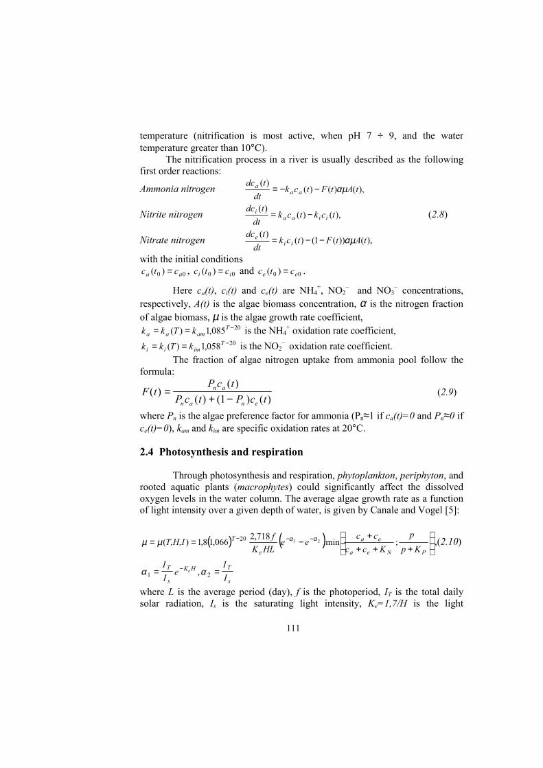
2.4 Photosynthesis and respiration

Through photosynthesis and respiration, phytoplankton, periphyton, androoted aquatic plants (macrophytes) could significantly affect the dissolvedoxygen levels in the water column. The average algae growth rate as a functionof light intensity over a given depth of water, is given by Canale and Vogel [5]:

( ) ( )

+++

+−== −−−

PNea

ea

e

T

Kpp

Kcccc

eeHLK

fT,H,I ;min718,2066,18,1)( 2120 ααµµ ,(2.10)

α α1 2= =−II e

II

T

s

K H T

s

e ,

where L is the average period (day), f is the photoperiod, IT is the total dailysolar radiation, Is is the saturating light intensity, Ke=1,7/H is the light

112

extinction coefficient, KN and KP is the half-saturation constant for nitrogen andphosphorus.

The approximate respiration rate is given by Thomann [2]20)08,1()( −== T

iT ρρρ (2.11)where iρ varies from 0,05 to 0,25. A value of 0,15 is usually used as a firstapproximation.

2.5 Point pollution sources

Applying equation (2.1), we use the standard time-distance change.Suppose that in a river stretch [ ]xx ,0 there is neither point nor distributedpollution sources. If at time t0 a water column with an oxygen concentration 0ocwere at a river section x0, i.e. 000 )()(~

ooo ctcxc == , then this water column willreach a river section x (downstream) at time vxxtt /)( 00 −+= ( v is the averageriver flow velocity in the stretch [ ]xx ,0 ), and its oxygen concentration will be

)(/)(()(~00 tcvxxtcxc ooo =−+= , the solution to equation (2.1) with the initial

condition 00 )( oo ctc = .All the tributaries with significant flow (exceeding a certain chosen

value ε) are regarded as point pollution sources. Calculating the oxygenconcentration after a point source, we assume that the river and tributary flowsare mixed immediately at the location of tributary, i.e. if a point source islocated at a river section x, then the oxygen concentration after the confluence,

)( +xco is given by

QxQQcxQxc

xc ooo ~)(

~~)()()(

+−+−−

=+

(2.12)

where ~Q and 0~c are the tributary flow and its oxygen concentration, while Q(x-

) and co(x-) are the river flow and its oxygen concentration before theconfluence. The same approach is applied to other concentrations.

Hence the point sources are included in the model as the new initialconditions considering river stretches between tributaries.

If there were no effluent discharge from the wastewater treatment plantat the end of first reach, all concentrations calculated at the end of the first reachwould have been used as boundary concentrations for the second reach.Because of the wastewater treatment plant discharge at x, all water qualityconstituent concentrations have to be calculated assuming a complete mixing ofeffluent water with stream water and the new values will be used as boundaryconcentrations to the second reach.

113

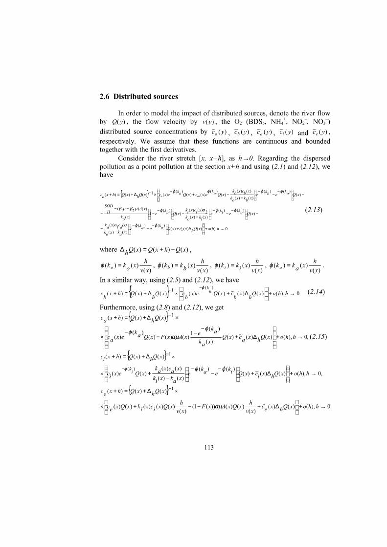
2.6 Distributed sources

In order to model the impact of distributed sources, denote the river flowby )(yQ , the flow velocity by )(yv , the O2 (BDS5, NH4

+, NO2–, NO3

–)distributed source concentrations by )(~ yco , )(~ ycb , )(~ yca , )(~ yci and )(~ yce ,respectively. We assume that these functions are continuous and boundedtogether with the first derivatives.

Consider the river stretch [x, x+h], as h→0. Regarding the dispersedpollution as a point pollution at the section x+h and using (2.1) and (2.12), wehave

{ }

0),()()(~)()()(

)()(1)(

)()()(

)()(2)()(

)()(

1)(

)()21(

)()()(

)()()()(

)()(

)()()(

)(1)()()(

→+

∆+

−−

−−

−

−

−−

−−

−

−−

−−−

−−

−−

−−+

−×−∆+=+

hhoxQhxcxQokeak

exakxok

(x)acαxak

xQokeik

exikxok

xicxikxQok

exok

xAH

SOD

xQokebk

exbkxok

xbcxbkxQok

excxQokexcxQhxQhxoc

o

oso

ϕϕ

ϕϕαϕρβµβ

ϕϕϕϕ

(2.13)

where )()()( xQhxQxQh −+=∆ ,

)()()(

xvhxokko =ϕ ,

)()()(

xvhxbkkb =ϕ ,

)()()(

xvhxikki =ϕ ,

)()()(

xvhxakka =ϕ .

In a similar way, using (2.5) and (2.12), we have

{ } 0),()()(~)()()()()()(1

→+∆+∆+=+

−

×− hhoxQ

hx

bcxQex

bcxQ

hxQhx

bc b

kϕ (2.14)

Furthermore, using (2.8) and (2.12), we get{ }

,0),()()(~)()(

)(1)()()(

)()(

1)()()(

→+

∆+−

−−−

×

×−∆+=+

hhoxQhxacxQxak

akexAxFxQak

exac

xQhxQhxac

ϕαµ

ϕ (2.15)

{ },0),()()(~)(

)()()()(

)()()()(

)()()(

)(

1

→+

∆+

−−

−−

+

∆+=+

−×

×−

hhoxQhxicxQikeak

exakxik

xacxakxQexic

xQhxQhxic

ik ϕϕϕ

{ }.0),()()(~

)()()())(1(

)()()()()()(

)()()( 1

→+

∆+−−+

∆+=+

×

×−

hhoxQhxecxv

hxQxAxFxv

hxQxicxikxQxec

xQhxQhxec

αµ

114

Using Taylor’ expansion and passing to the limit as h→0, we obtain thefollowing first-order differential equations:

[ ] 01)(~2121 =

−−++++−+

′−++′

v(x)ρ)A(x)βμ(β(x)cαk(x)cαk

HSOD(x)ckxck

Q(x)(x)Q(x)c(x)c

v(x)(x)k

(x)c(x)c iiaabbosoooo

oo

[ ] 0)()(

)(~)()()(

)()( =′

−++′xQxQxbcxbc

xvxk

xbcxbc b ,

[ ] ,0)(

1)()()()(

)(~)()()(

)()( =+′

−++′xv

xAxFxQxQxacxac

xvxk

xacxac a αµ (2.16)

[ ] ,0)(

)()(

)()(

)(~)()()(

)()( =−′

−++′xv

xacxak

xQxQxicxic

xvxk

xicxic i

[ ] ( ) .0)(

1)()()())(1()()(

)(~)()( =−−+′

−+′xv

xicxikxAxFxQxQxecxecxec αµ

The flow may be related to river basins area from which all the pointsources are exclude.

Consider the river stretch [ ]10 , xx where there is no point sourceloading. We assume that the river flow and the basin area are described bybounded and continuously differentiable functions )(yf and )(yg , i.e.

))()(()()( 00 xAxAfxQxQ −=− , (2.17))()()( 00 xxgxAxA −=− , [ ]10 , xxx ∈ .

Then( )

))()(()()()()(

)()(

00

00

xAxAfxQxxgxAxAf

xQxQ

−+−′−′

=′ . (2.18)

If we assume that f and g are linear functions, i.e.yyf β=)( , yyg η=)( ,

then

))()(()()()(

00 xxxAxQxQxQ

−++=

′ηβ

βη . (2.19)

Hence, applying a linear approximation to the river stretch [ ]10 , xx , thecoefficients β and η are defined by

)()()(

)()()()(

01

01

01

01

xxxQxQ

xAxAxQxQ

−−

=−−

=η

β

and

01

01 )()(xx

xAxA−−

=η (2.20)

115

We assume that the distributed source and the basin area are describedby bounded and continuously differentiable function )(yh , i.e.

))()(()(~)(~00 xAxAhxcxc −=− . (2.21)

3 Model adaptation

The mathematical model for dissolved oxygen balance (2.16) isinvolved therefore we simplify it. Consider the river stretch [ ]xx ,0 we assumethe initial condition:

constxko ≡)( , constxkb ≡)( , constxki ≡)( , constxka ≡)( , constxv ≡)( ,constxc ≡)(~ .

According to the State Monitoring Programme, BDS5, NH4+, NO2

−, NO3– and O2

are measured in five sections P1-P5 of the Neris and four sections Z1-Z4 ofŽeimena (Fig. 3.1) once per month. The sewage disposal of the townsNemenčinė, Pabradė, Švenčionėliai, Jonava and the city of Vilnius is subjectedto laboratory monitoring.We have analysed seven river stretches, namely, P1-P2, P2-P3, P3-P4, P4-P5,and Z1-Z2, Z2-Z3, Z3-Z4. Stretches P1-P2 and Z1-Z2 are the least affected byanthropogenic activity, and for this reason they serve best for the adaptation of amathematical model and calculation of its coefficients. The mathematical modeladapted for the first stretch is then applied to other stretches.

Fig.3.1. State monitoring sections (1996).

226 km P1

184 km P2

141 km P3

51.5 kmP4

35.5 kmP5Jonava 39 km T4

“Achema” 44 km T3

Vilnius 148 km T2

Nemenčinė 197 km T1

Šventoji 44.5 km

Žeimena 212.6 km

Nemunas

Z4 Z3 Z2 Z178,6 km52,7 km20 km13,7 km

Pabr

adė

19 k

m

Švenči

onėl

iai 5

5 km

Baltarusijos Respublika

116

Model adaptation is the first stage of testing and tuning a model to a setof field data, preferably a set of field data not used in the original modelconstruction. The distributed source, chemical and biological kineticcoefficients may be determined from statistical analysis.

Adapting water quality model, the analyst selectively determines somemodel-input parameters that, when used in the model, yield reasonablesimulations of observed water quality data. Some of these input parameters,such as Q, v , BDS5, NH4

+, NO2–, NO3

–, O2, Cl, T and solar energy are directlymeasured. Other model parameters, such as oxidation rates, reaeration rates,nitrification rates, SOD, distributed source, distributed flow, and algae are notdirectly measured. These parameters are determined by empirical formulas andtheir values are obtained in the process of model adaptation. The decompositionrate coefficient, reaeration rates coefficients, distributed flow, SOD and algaeare determined from empirical formulas. The distributed sources concentrationand oxidation rates coefficients are determined by model adaptation (i.e. interms of the least square deviation)

( )ia kkc

N

iii tctc

,,~1

2 min)(~)( →−∑=

, (3.1)

where )( itc is the measured concentration and )(~itc is the value obtained from

the model, both at time it .Goodness of fit of the model and the field data are measured by the

correlation coefficient

( )( )

( ) ( )∑ ∑

∑

= =

=

−−

−−

=N

i

N

iii

N

iii

ctcctc

ctcctcr

1 1

22

1

)(~)(~

~)(~)(

(3.2)

and the determination coefficient

( )

( )∑

∑

=

=

−

−= N

ii

N

iii

tc

tctcR

1

2

1

2

2

)(

)(~)(

1 (3.3)

where ∑=

=N

iitc

Nc

1

)(1 and ∑=

=N

iitc

Nc

1

)(~1~ .

117

On the basis of long-term hydrological and hydrochemical statemonitoring data for the Neris River and the Žeimena River, the dependence ofdissolved oxygen on the biochemical oxygen demand, nitrification, reaeration,sedimentation, photosynthesis and algae respiration are studied.

Modelling the stretch P1-P2 and assessing the Žeimena River and thetown of Nemenčine, we obtain that the NH4

+ correlation coefficient r is 0,98;NO2

– - 0,98; NO3– – 0,95; BDS5 – 0,94 and O2 – 0,74 (table 3.1).

When data from a winter survey are first used to calibrate a model, thedissolved oxygen balance is not sensitive to the nitrification rate and, therefore,decomposition rate and distributed source can be determined more accurately.During model validation, another set of data collected in the summer months isused. Since the nitrification process is highly sensitive to the temperature, themodelling analysis is able to tune the nitrification rate with greater accuracy.Then, in winter months error of estimate is smaller than in summer months.

Without assessing the BDS5 distributed sources, we obtain that theBDS5 determination coefficient is 1,14 time smaller than for simulation throughthe assessment of distributed sources [11]. The NH4

+ determination coefficientis 1,18 (NO2

– gives 1,22, NO3– gives 1,07) time smaller than for simulation

through the assessment of distributed sources and algae quantity [12].Recall that for the stretch immediately below the discharge, biological

activity is primarily heterotrophic. That is, it is dominated by organisms such asbacteria that obtain their energy by consuming organic matter, and in theprocess, deplete oxygen. Plant growth in this area is suppressed because of anumber of factors, including light extinction due to turbidity.

Further downstream, as the stream begins to recover, levels of nutrientssuch as organic matter (nitrogen, phosphorus) will be high.

Because photosynthesis is light dependent, this effect can haveseasonality.

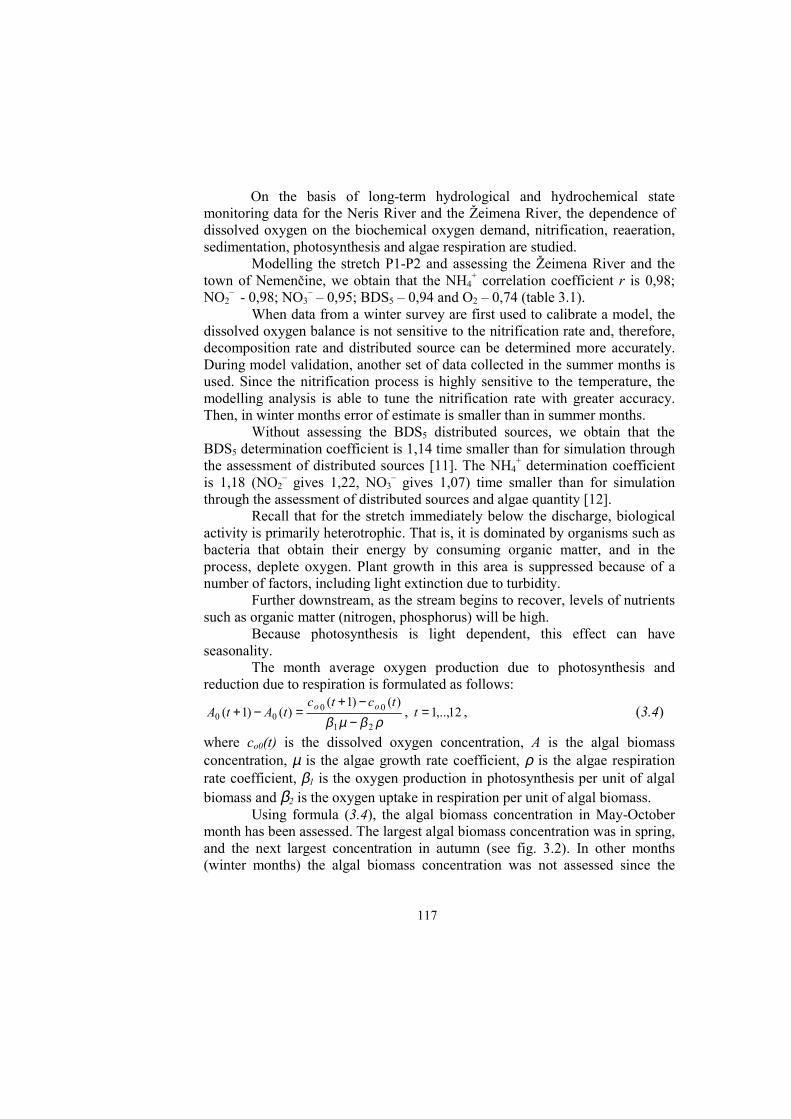
The month average oxygen production due to photosynthesis andreduction due to respiration is formulated as follows:

ρβµβ 21

0000

)()1()()1(

−−+

=−+tctc

tAtA oo , 12,..,1=t , (3.4)

where co0(t) is the dissolved oxygen concentration, A is the algal biomassconcentration, µ is the algae growth rate coefficient, ρ is the algae respirationrate coefficient, β1 is the oxygen production in photosynthesis per unit of algalbiomass and β2 is the oxygen uptake in respiration per unit of algal biomass.

Using formula (3.4), the algal biomass concentration in May-Octobermonth has been assessed. The largest algal biomass concentration was in spring,and the next largest concentration in autumn (see fig. 3.2). In other months(winter months) the algal biomass concentration was not assessed since the

118

water temperature and light energy was lower, which means that algal biomassgrows slowly or even does not grow at all.

There are two peaks in figure 3.2. In winter months algal biomassgrowth is slow, since water temperature and light intensity is low, but there is alarge amount of accumulated organic matter in the water. Water temperatureand light intensity determine the fast algal biomass growth, because biogenicmatter (spring flowering) does not limit them. The fast decrease of organicmatters, determine the end of flowering and accumulation of organic matter inthe water. Then the algal biomass grows fast, i.e. the autumn flowering willcontinue while the limit factor of algal biomass growth appears (lower watertemperature and light intensity).

Fig.3.2. Mean algae concentrations in the section P2 1991-1997 m.(♦ - section P1; ■ - section Z1)

The simulation of O2, without nitrification, algal respiration andphotosynthesis assessment, we obtain 1,13 times smaller correlation coefficient.In particular, the process of nitrification as well as the algal affects dissolvedoxygen during the warmer period, i.e. without assessing nitrification and algaewe have 1,45 times smaller correlation coefficient in May - August.

The NH4+, NO3

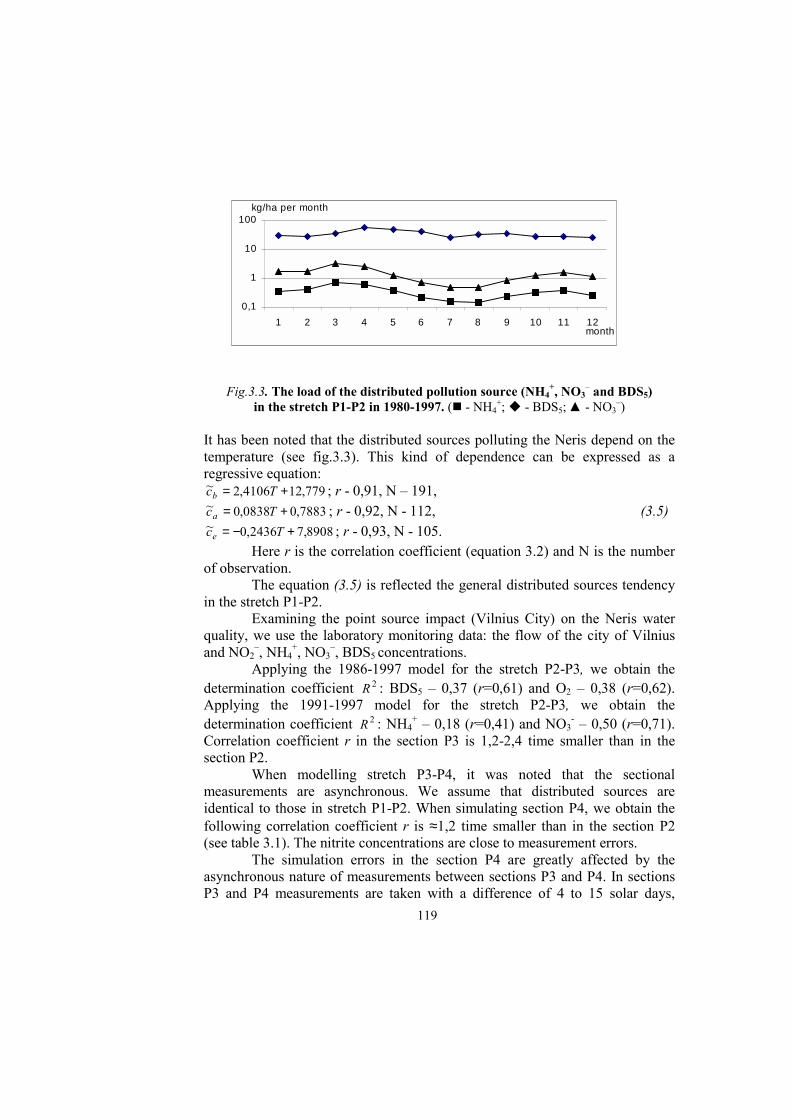
– and BDS5 distributed pollution source has beencalculated according to pollution mass balance formula (2.12) in the stretch P1-P2. The largest load of the distributed NH4

+ (NO3– and BDS5) source is in

March-May. The NH4+ distributed source is 0,74 and 0,63 kgN/ha month (NO3

–-3,17 and 2,52kgN/ha month, BDS5 – 59 and 51 kgO2/ha in month.). Thesmallest load is in July-August (NH4

+ – 0,15 kgN/ha month; NO3– - 0,47 kgN/ha

month; BDS5 – 26 and 32 kgO2/ha month) (Fig. 3.3). The yearly load of thedistributed NH4

+ source is 4,3 kgN/ha year, NO3– - 17 kgN/ha year and BDS5 –

424 kgO2/ha year.

02468

1012

1 2 3 4 5 6 7 8 9 10 11 12

m g/ l

m onth

119

Fig.3.3. The load of the distributed pollution source (NH4+, NO3

– and BDS5)in the stretch P1-P2 in 1980-1997. (! - NH4

+; " - BDS5; ▲ - NO3–)

It has been noted that the distributed sources polluting the Neris depend on thetemperature (see fig.3.3). This kind of dependence can be expressed as aregressive equation:

779,124106,2~ += Tcb ; r - 0,91, N – 191,7883,00838,0~ += Tca ; r - 0,92, N - 112, (3.5)

8908,72436,0~ +−= Tce ; r - 0,93, N - 105.Here r is the correlation coefficient (equation 3.2) and N is the number

of observation.The equation (3.5) is reflected the general distributed sources tendency

in the stretch P1-P2.Examining the point source impact (Vilnius City) on the Neris water

quality, we use the laboratory monitoring data: the flow of the city of Vilniusand NO2

–, NH4+, NO3

–, BDS5 concentrations.Applying the 1986-1997 model for the stretch P2-P3, we obtain the

determination coefficient 2R : BDS5 – 0,37 (r=0,61) and O2 – 0,38 (r=0,62).Applying the 1991-1997 model for the stretch P2-P3, we obtain thedetermination coefficient 2R : NH4

+ – 0,18 (r=0,41) and NO3- – 0,50 (r=0,71).

Correlation coefficient r in the section P3 is 1,2-2,4 time smaller than in thesection P2.

When modelling stretch P3-P4, it was noted that the sectionalmeasurements are asynchronous. We assume that distributed sources areidentical to those in stretch P1-P2. When simulating section P4, we obtain thefollowing correlation coefficient r is ≈1,2 time smaller than in the section P2(see table 3.1). The nitrite concentrations are close to measurement errors.

The simulation errors in the section P4 are greatly affected by theasynchronous nature of measurements between sections P3 and P4. In sectionsP3 and P4 measurements are taken with a difference of 4 to 15 solar days,

0,1

1

10

100

1 2 3 4 5 6 7 8 9 10 11 12

kg/ha per month

month

120

which accounts for the fact that the monitoring data mayn’t reflect actualdynamics (i.e. they mayn’t reflect actual organic pollution dependence betweenthe sections). It is only with the change of the state monitoring system that theparameters could be assessed with a sufficient degree of accuracy (i.e. in respectto distance and flow rate, measurements in the section P4 should be taken afterone to three solar days compared to those in the section P3).

Applying the model for section P5 of the years 1991-1997 in pollutionload assessment for the town of Jonava and for “ACHEMA” company, weobtain the correlation coefficient r in the section P5 is ≈1,6 time smaller than inthe section P2 (see table 3.1).

When modelling the Žeimena River, we obtain the averagedetermination coefficient 2R in the sections Z2-Z4 is NH4

+ - 0,86; NO3– - 0,83;

BDS5 – 0,72 and O2 – 0,68 (Table 3.1). The nitrite concentrations are close tomeasurement errors.

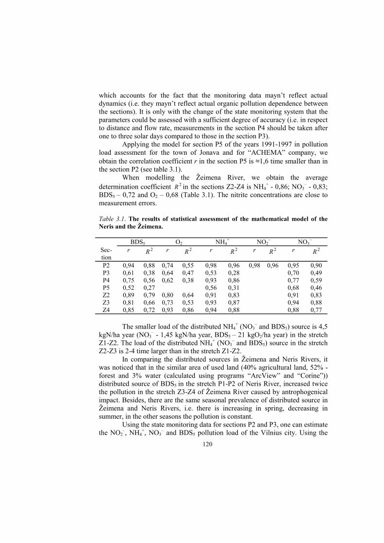
Table 3.1. The results of statistical assessment of the mathematical model of theNeris and the Žeimena.

BDS5 O2 NH4+ NO2

– NO3–

Sec-tion

r 2R r 2R r 2R r 2R r 2R

P2 0,94 0,88 0,74 0,55 0,98 0,96 0,98 0,96 0,95 0,90P3 0,61 0,38 0,64 0,47 0,53 0,28 0,70 0,49P4 0,75 0,56 0,62 0,38 0,93 0,86 0,77 0,59P5 0,52 0,27 0,56 0,31 0,68 0,46Z2 0,89 0,79 0,80 0,64 0,91 0,83 0,91 0,83Z3 0,81 0,66 0,73 0,53 0,93 0,87 0,94 0,88Z4 0,85 0,72 0,93 0,86 0,94 0,88 0,88 0,77

The smaller load of the distributed NH4+ (NO3

– and BDS5) source is 4,5kgN/ha year (NO3

– - 1,45 kgN/ha year, BDS5 – 21 kgO2/ha year) in the stretchZ1-Z2. The load of the distributed NH4

+ (NO3– and BDS5) source in the stretch

Z2-Z3 is 2-4 time larger than in the stretch Z1-Z2.In comparing the distributed sources in Žeimena and Neris Rivers, it

was noticed that in the similar area of used land (40% agricultural land, 52% -forest and 3% water (calculated using programs “ArcView” and “Corine”))distributed source of BDS5 in the stretch P1-P2 of Neris River, increased twicethe pollution in the stretch Z3-Z4 of Žeimena River caused by antrophogenicalimpact. Besides, there are the same seasonal prevalence of distributed source inŽeimena and Neris Rivers, i.e. there is increasing in spring, decreasing insummer, in the other seasons the pollution is constant.

Using the state monitoring data for sections P2 and P3, one can estimatethe NO2

–, NH4+, NO3

– and BDS5 pollution load of the Vilnius city. Using the

121

equation (2.12), we obtain( )

QxQxcQxQxc

c ~)()(~)()(~ 0000 −−−+−+

=,

(3.6)

where Q~ and c~ are the point flow and BDS5 (NH4+, NO2

–, NO3–)

concentration, while Q(x0-), c(x0-) and c(x0+) stand for the river flow, BDS5(NH4

+, NO2–, NO3

–) concentration before the confluence and after it.The calculated NO2

– and NH4+ pollution loads for 1980-1997 differ

about 15%, NO3– about 26% and BDS5 about 18% from the Vilnius sewage

disposal laboratory monitoring data (Fig.3.4) [11, 12].NH4

+ and NO2– oxidation rate coefficients (ka and ki) before and after

the purification plants of the city of Vilnius were fluctuating in the range 0,04-0,29 and 0,1-0,65, 0,84-2,86 and 0,48-1,7 d-1.

Fig.3.4. Estimated BDS5 pollution load brought from the Vilnius city purificationplants in the years 1987-1996.

( - data from the Sewage Laboratory of Vilnius city. ! - model estimates based on themonitoring data in sections P2 and P3)

Using the state monitoring data for sections P4 and P5, may be estimatethe NO2

–, NH4+, NO3

– and BDS5 pollution load of the Jonava city and the“ACHEMA” company.

4 Time series analysis

In order to establish the long-term tendencies of the water qualityparameters, i.e. the concentrations of BDS5, NO3

–, NH4+ and O2, we apply the

standard time series modeltttt YSmX ++= , Nt ,...,1= . (4.1)

Here tm is a deterministic trend, tS is a deterministic seasonalcomponent with the natural period T of 12 months (T=12, Ttt SS += and

0

5 0 0 0

1 0 0 0 0

1 5 0 0 0

2 0 0 0 0t /y ear

122

01

=∑=

+

T

jtjS , t∀ ), tY is a random component, and N is the number of

observations.

When analysing the time series of NH4+ in the Neris River, we replace

tX in (4.1) by)ln( tt XZ = . (4.2)

Since N the number of observations of the time series analysed, iscomparatively small, it is reasonable to use trend models containing only a fewparameters to be identified. We apply a linear model for the trend, i.e.

btamt += , (4.3)where a and b are unknown coefficients.

The coefficients of deterministic components ( tm and tS ) are estimatedby the Ordinary Least-Squares method (OLS).

Denote by tm and tS the estimated trend and seasonal components. Forthe series:

tttt SmXY ˆˆˆ −−= , (4.4)we apply the autoregressive moving average (ARMA) model:

∑∑=

−=

− +=+q

jjtit

p

iitit dYcY

11

ˆˆ εε , ,,...,1,0 Nt = (4.5)

where tε is a white noise series.The coefficients ic and id are estimated using the OLS method

(statistical package STATISTICA 5.0).The p–value is used in the package to evaluate the null hypothesis

validity.Recall that the p–value is the probability that the t-statistic (in the case,

when 0H is true) is not less than the observed value of the t-statistic.Let α denote a significance level and p denote a p–value. The

hypothesis 0H is accepted if α≥p , and is rejected otherwise.For testing the null hypothesis 0=b ( 0H : 0=b ) agains the alternatyve

0≠b ( 1H : 0≠b ) we use t - statistic and standart significance level α=0,05. Forthe BDS5, we obtain that the null hypothesis is accepted (p–value is 9,03,0 ÷ ).

The parameter a is estimated by ∑=

=N

ttX

Na

1

1ˆ .

123

By N we denote the number of complete periods, so that na ,...,1= . Given thisnotation, a sequence tX ( Nt ,...,1= ) can be written as paiX + ( pi ,...,1= ,

na ,...,1= ).The seasonal coefficients is of tS are calculated as follows:

∑=

++ −=n

apaipaii mX

ns

1

)ˆ(1ˆ . (4.6)

In fig. 4.1, the BDS5 time series seasonal coefficients is in the Nerisand the Žeimena are plotted. Statistical analysis shows that the seasonalcoefficients )3P(12s , )4P(9s , )1Z(7s , )1Z(12s , )2Z(2s , )2Z(7s , )3Z(7s , )4Z(2s ,

)4Z(5s , )4Z(6s , )4Z(7s , )4Z(10s , and )4Z(11s are statistically insignificant atthe 0,05 significance level (p–values are 0,42, 0,31, 0,85, 0,69, 0,65, 0,48, 0,12,0,12, 0,15, 0,9, 0,64, 0,6, and 0,45, respectively). The remaining seasonalcoefficients are statistically significant at the 0,05 significance level.

Fig.4.1. The seasonal coefficients is . (◊ in the sections P1, P2, Z1 and Z2; ∆ in thesections P3 and Z3; □ in the sections P4, P5 and Z4, respectively)

In order to test hypothesis about ARMA coefficients significantlyanalysis of ARMA coefficients, we assume that the series tY is Gaussian.

-3

-2

-1

0

1

2

3

4

5

1 2 3 4 5 6 7 8 9 10 11 12

Neris

m onth

m gO 2/ l

-0,8

-0,6

-0,4

-0,2

0

0,2

0,4

0,6

1 2 3 4 5 6 7 8 9 10 11 12

m gO 2/ l Zeimena

m onth

124

For the series tY , we can define its autocorrelation function is definedby:

)(ˆ)(ˆ)(ˆ stYtYEsRY += , t∀ . (4.7)It’s necessary to emphasize, that p-values are calculated according to

supposition, that tY is white Gaussian noise, wich isn’t correct, as it showsfurther statistical analysis.

Statistical analysis of series tY shows that YR ˆ has a positive peak at lag1, i.e. )1(YR is 0,2 in section P1, 0,19 in section P2, 0,27 in section P3, 0,45 insection P4, and 0,26 in section P5 and all them are non zero with thesignificance level α=0,05 (N=96). For the Žeimena, the )1(YR in all sectionsassumes small value in a ranging from 0,08 to 0,14 and can be assumed to bezero (p=0,3). Thus, for the series tY the model is that of AR(1) in the NerisRiver and a pure white noise in the Žeimena River.

Thus, for the series tY , the chosen model is AR(1). For this model theMean Square Error (MSE) is 3,73 in the section P1, 2,93 in the section P2, 6,06in the section P3, 4,35 in the section P4 and 2,87 in the section P5.

Finally, the statistical analysis of the residual series tε shows that)(tRε , 0>t , can be assumed to be zero ( 92,03,0 ÷=p ). Hence, the series tε is

actually a pure white noise.Hence, the estimated model for the BDS5 can be written as:

P1: tit Ys,X ˆ)1P(ˆ313ˆ ++= , ttt εY,Y ˆˆ20ˆ1 =+ − , (4.8)

P2: tit YsX ˆ)2P(ˆ13,3ˆ ++= , ttt εY,Y ˆˆ190ˆ1 =+ − ,

P3: tit YsX ˆ)3P(ˆ42,6ˆ ++= , ttt εY,Y ˆˆ270ˆ1 =+ − ,

P4: tit YsX ˆ)4P(ˆ26,5ˆ ++= , ttt εY,Y ˆˆ450ˆ1 =+ − ,

P5: tit YsX ˆ)5P(ˆ14,4ˆ ++= , ttt εY,Y ˆˆ260ˆ1 =+ − ,

Z1: tit YsX ˆ)1Z(ˆ59,1ˆ ++= , ttY ε=ˆ ,Z2: tit YsX ˆ)2Z(ˆ68,1ˆ ++= , ttY ε=ˆ ,Z3: tit YsX ˆ)3Z(ˆ6,1ˆ ++= , ttY ε=ˆ ,Z4: tit YsX ˆ)4Z(ˆ8,1ˆ ++= , ttY ε=ˆ .

The seasonal coefficients )P1(ˆis , )2P(ˆis , )3P(ˆis , )4P(ˆis , )5P(ˆis ,)1Z(ˆis , )2Z(ˆis , )3Z(ˆis and )4Z(ˆis are given in the table 4.1.

125

Table 4.1. The seasonal coefficients )P1(ˆis - )5P(ˆis and )1Z(ˆis - )4Z(ˆis .Month I II III IV V VI VII VIII IX X XI XII

BDS5

)P1(ˆis -1,86 -1,38 -0,73 -0,90 2,53 1,69 2,54 2,41 -0,54 -0,85 -1,46 -1,45

)2P(ˆis -1,66 -1,67 -0,98 -0,72 2,65 2,29 2,13 2,27 -0,70 -0,93 -1,20 -1,47

)3P(ˆis -2,23 -1,42 -0,50 -1,61 3,75 4,30 1,51 1,23 -0,81 0,19 -1,80 -2,61

)4P(ˆis -2,56 -1,87 -1,16 -1,41 3,30 3,28 3,81 1,96 -0,27 -1,53 -1,15 -2,41

)5P(ˆis -1,83 -1,21 -0,89 -0,68 1,31 3,48 3,67 2,47 -0,50 -1,96 -1,78 -2,07

)1Z(ˆis -0,23 0,45 -0,24 0,07 0,81 0,04 0,08 -0,33 -0,29 -0,04 -0,24 -0,08

)2Z(ˆis -0,29 0,03 -0,24 0,33 0,50 0,51 0,05 -0,53 -0,44 0,17 -0,34 0,25

)3Z(ˆis -0,13 0,41 0,01 0,05 0,35 0,32 -0,08 -0,12 -0,39 -0,32 -0,18 0,08

)4Z(ˆis -0,37 0,04 -0,55 0,32 0,27 0,09 -0,05 0,02 0,08 0,12 -0,05 0,07

NO3–

)P1(ˆis 0,42 0,51 0,33 0,34 -0,31 -0,41 -0,40 -0,32 -0,26 -0,15 0,03 0,22

)2P(ˆis 0,48 0,37 0,22 -0,35 -0,48 -0,46 -0,31 -0,13 -0,08 0,14 0,20 0,41

)3P(ˆis 0,37 0,40 0,32 0,30 -0,39 -0,56 -0,45 -0,39 -0,21 -0,07 0,21 0,48

)4P(ˆis 0,67 0,79 0,76 0,24 -0,55 -0,75 -0,63 -0,76 -0,44 0,09 0,15 0,42

)5P(ˆis 0,79 0,81 0,61 0,26 -0,17 -0,55 -0,78 -0,81 -0,62 -0,26 0,17 0,55

)1Z(ˆis 0,05 0,27 0,18 0,13 -0,04 -0,02 -0,17 -0,16 -0,14 -0,14 -0,01 0,05

)2Z(ˆis 0,18 0,26 0,18 0,11 -0,13 -0,10 -0,17 -0,18 -0,14 -0,08 0,00 0,09

)3Z(ˆis 0,15 0,14 0,26 0,08 -0,12 -0,13 -0,23 -0,17 -0,15 -0,07 0,11 0,13

)4Z(ˆis 0,14 0,12 0,18 0,05 -0,14 -0,08 -0,22 -0,15 -0,14 -0,06 0,06 0,24

NH4+

)P1(ˆis 0,28 0,55 0,65 0,14 -0,61 -0,34 -0,87 -0,58 -0,19 0,71 0,04 0,22

)2P(ˆis 0,89 0,72 0,41 0,00 -0,15 -0,25 -0,76 -0,82 -0,56 -0,29 0,17 0,63

)3P(ˆis 0,68 0,76 0,35 0,16 -0,23 -0,55 -0,53 -0,75 -0,37 -0,14 0,19 0,42

)4P(ˆis 0,43 0,26 0,51 -0,06 0,04 -0,29 -0,34 -0,72 -0,55 0,00 0,33 0,39

)5P(ˆis 0,43 0,26 0,51 -0,06 0,04 -0,29 -0,34 -0,72 -0,55 0,00 0,33 0,39

)1Z(ˆis 0,04 0,01 0,01 -0,01 -0,01 0,01 -0,03 -0,01 -0,03 0,01 0,01 0,01

)2Z(ˆis 0,03 0,04 0,01 -0,01 -0,02 -0,02 -0,02 -0,03 -0,02 0,01 0,01 0,04

)3Z(ˆis 0,02 0,04 0,02 -0,01 -0,03 0,00 -0,03 -0,03 -0,02 0,01 0,02 0,03

)4Z(ˆis 0,03 0,05 0,01 -0,01 -0,02 -0,04 -0,02 -0,04 -0,03 0,01 0,02 0,03

O2

)1Z(ˆis 0,19 0,09 1,26 1,46 0,43 -0,62 -0,57 -1,17 -0,77 -0,52 -0,18 0,40

)2Z(ˆis 0,27 0,15 1,21 0,90 -0,03 -0,52 -1,01 -0,97 -0,42 -0,04 -0,16 0,62

)3Z(ˆis 0,23 0,03 1,30 0,57 -0,14 -0,51 -1,01 -0,51 -0,34 0,06 -0,10 0,43

)4Z(ˆis 0,23 0,06 1,30 0,35 -0,36 -0,41 -1,34 0,03 -0,20 -0,04 0,01 0,38

126

The same statistical analysis for the NO3– shows that the null hypothesis

0H : 0=b is accepted (p–value is 82,012,0 ÷ , α is 0,05). Thus, the trend is

∑=

==N

ttt X

Nam

1

1ˆˆ .

Fig. 4.2 represents the NO3– seasonal coefficients is in the Neris and

the Žeimena. Statistical analysis shows that the seasonal coefficients )2P(10s ,)3P(10s , )5P(10s , )4P(4s , )4P(10s , )4P(11s , )1Z(3s , )1Z(4s , )1Z(10s , )2Z(9s ,)4Z(4s , and )4Z(9s are statistically insignificant at the 0,05 significance level

(p–values are 0,38, 0,36, 0,32, 0,47, 0,28, 0,09, 0,63, 0,89, 0,24, 0,78, 0,09, and0,13, respectively). The remaining seasonal coefficients are statisticallysignificant at the 0,05 significance level.

Fig.4.2. The seasonal coefficients is .(◊ in the sections P1-P3, Z1 and Z2; □ in the sections P4, P5, Z3 and Z4, respectively)

After estimation of the components (trend and seasonal), and thecomputation of the residuals. The series tY autocorrelation function )(ˆ sRY

showed significant peaks at lags 1 at the α=0,05 in the sections P1-P5 and Z3-Z4. The )(ˆ sRY in the sections Z1-Z2 reveals a pure white noise.

For the series tY the model AR(1) can be chosen. For this model theMSE are 0,049 in the section P1, 0,054 in the section P2, 0,04 in the section P3,0,17 in the section P4, 0,2 in the section P5, 0,028 in the section Z3 and 0,023 inthe section Z4. The statistical analysis of the residual series tε shows that

0)( =tRε , 0>t , ( 87,073,0 ÷=p ). Thus, the series tε is actually a pure whitenoise. Hence, the estimated model for the NO3

– can be written as:P1: tit YsX ˆ)P1(ˆ68,0ˆ ++= , ttt YY εˆ46,0ˆ

1 =+ − , (4.9)P2: tit YsX ˆ)P2(ˆ69,0ˆ ++= , ttt YY εˆ36,0ˆ

1 =+ − ,

-0,3

-0,2

-0,1

0

0,1

0,2

0,3

1 2 3 4 5 6 7 8 9 10 11 12

m gN / l Zeimena

m onth

127

P3: tit YsX ˆ)P3(ˆ79,0ˆ ++= , ttt YY εˆ23,0ˆ1 =+ − ,

P4: tit YsX ˆ)P4(ˆ94,0ˆ ++= , ttt YY εˆ54,0ˆ1 =+ − ,

P5: tit YsX ˆ)P5(ˆ04,1ˆ ++= , ttt YY εˆ53,0ˆ1 =+ − ,

Z1: tit YsX ˆ)Z1(ˆ38,0ˆ ++= ttY ε=ˆ ,Z2: tit YsX ˆ)2Z(ˆ42,0ˆ ++= , ttY ε=ˆ ,Z3: tit YsX ˆ)3Z(ˆ47,0ˆ ++= , ttt YY εˆ23,0ˆ

1 =+ − ,Z4: tit YsX ˆ)4Z(ˆ51,0ˆ ++= , ttt YY εˆ22,0ˆ

1 =+ − .The seasonal coefficients )P1(ˆis , )2P(ˆis , )3P(ˆis , )4P(ˆis , )5P(ˆis ,

)1Z(ˆis , )2Z(ˆis , )3Z(ˆis and )4Z(ˆis are given in the table 4.1.When examining the ammonia nitrogen (NH4

+) time series in the NerisRiver (sections P1-P5) we observe that it is difficult to separate the seasonalcomponent from the data. Therefore, we first perform the following datatransformation. For the Žeimena, the NH4

+ time series of sections Z1-Z4 areanalysing by equation (4.1).

For the NH4+ we obtain that 0H : 0=b , 0=c is rejected in sections P1-

P5 and Z4 (the significance level α=0,05 is greater than p-value of 0,002) and isaccepted in sections Z1-Z3 (p≥α, i.e. p=0,1, α=0,05). Thus, we reject the nullhypothesis that the series has a linear trend btamt += (P1-P3, Z4) andparabolic trend 2ctbtamt ++= (P4 and P5).

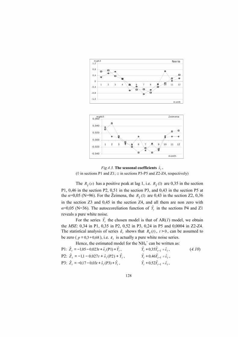
Fig. 4.3 represents the NH4+ time series seasonal coefficients is in the

Neris and the Žeimena. Statistical analysis shows that the seasonal coefficientsfor the Neris )1P(4s , )3P(4s , )3P(9s , )3P(10s , )3P(12s , )4P(9s , )4P(10s ,

)5P(4s , )5P(5s , and )5P(10s are statistically insignificant at the 0,05significance level (p–values are 0,6, 0,16, 0,32, 0,83, 0,06, 0,36, 0,99, 0,94,0,27, and 0,99, respectively). The other seasonal coefficients are statisticallysignificant at the 0,05 significance level. The seasonal coefficients for theŽeimena )2Z(2s , )2Z(8s , )3Z(2s , )4(2 Zs , )4Z(6s , and )4(8 Zs are statisticallysignificant (p–values are 0,02, 0,03, 0,04, 0,04, 0,02, 0,03, and 0,04,respectively), and the other seasonal coefficients are statistically insignificant(p–value is 95,007,0 ÷ ) at the 0,05 significance level.

128

Fig.4.3. The seasonal coefficients is .(◊ in sections P1 and Z1; □ in sections P3-P5 and Z2-Z4, respectively)

The )(ˆ sRY has a positive peak at lag 1, i.e. )1(YR are 0,35 in the sectionP1, 0,46 in the section P2, 0,51 in the section P3, and 0,43 in the section P5 atthe α=0,05 (N=96). For the Žeimena, the )1(YR are 0,43 in the section Z2, 0,36in the section Z3 and 0,45 in the section Z4, and all them are non zero withα=0,05 (N=36). The autoccoreliation function of tY in the sections P4 and Z1reveals a pure white noise.

For the series tY the chosen model is that of AR(1) model, we obtainthe MSE: 0,34 in P1, 0,35 in P2, 0,52 in P3, 0,24 in P5 and 0,0004 in Z2-Z4.The statistical analysis of series tε shows that )(tRε , 0>t , can be assumed tobe zero ( 68,03,0 ÷=p ), i.e. tε is actually a pure white noise series.

Hence, the estimated model for the NH4+ can be written as:

P1: tit Yst,,Z ˆ)P1(ˆ0230051ˆ ++−−= , ttt εY,Y ˆˆ350ˆ1 =−+ , (4.10)

P2: tit Yst,,Z ˆ)P2(ˆ027011ˆ ++−−= , ttt εY,Y ˆˆ460ˆ1 =−+ ,

P3: tit Yst,,Z ˆ)P3(ˆ030170ˆ ++−−= , ttt εY,Y ˆˆ520ˆ1 =−+ ,

- 1,2

- 0,8

- 0,4

0

0,4

0,8

1,2

1 2 3 4 5 6 7 8 9 10 11 12

m gN /l Ne r is

m onth

-0,040

-0,020

0,000

0,020

0,040

0,060

1 2 3 4 5 6 7 8 9 10 11 12

m gN / l Z eim ena

m onth

129

P4: tit Yst,t,,Z ˆ)P4(ˆ00060050062ˆ 2 ++−−−= , ttY ε=ˆ ,P5: tit Yst,t,,Z ˆ)P5(ˆ00040030771ˆ 2 ++−+−= , ttt εY,Y ˆˆ450ˆ

1 =−+ ,

Z1: tit YsX ˆ)Z1(ˆ05,0ˆ ++= , ttY ε=ˆ ,Z2: tit YsX ˆ)2Z(ˆ048,0ˆ ++= , ttt εY,Y ˆˆ430ˆ

1 =−+ ,Z3: tit YsX ˆ)3Z(ˆ044,0ˆ ++= , ttt εY,Y ˆˆ370ˆ

1 =−+ ,Z4: tit YstX ˆ)4Z(ˆ0011,0074,0ˆ ++−= , ttt εY,Y ˆˆ450ˆ

1 =−+ .The seasonal coefficients )P1(ˆis , )2P(ˆis , )3P(ˆis , )4P(ˆis , )5P(ˆis ,

)1Z(ˆis , )2Z(ˆis , )3Z(ˆis and )4Z(ˆis are given in the table 4.1.Further, we consider the time series of dissolved oxygen (O2) in the

Neris River. It has been noted that the time series has no seasonal component( 0≡tS ).

Now, usual t – statistic for 0H : 0=b reveals that the null hypothesiscan be accepted in sections P3-P5 and Z1-Z4 (p–value is 9,014,0 ÷ ) and isrejected in sections P1 and P2 (p–value is 0,006) at the 0,05 significance level.Thus, we have linear trend only in the sections P1 and P2.

Fig. 4.4 represents the O2 seasonal coefficients is in the Žeimena.Statistical analysis shows that the seasonal coefficients )1Z(1s , )1Z(2s , )1Z(11s ,

)2Z(5s , )2Z(10s , )2Z(11s , )3Z(2s , )3Z(5s , )3Z(10s , )3Z(11s , )4Z(2s , and)4Z(8s - )4Z(11s are statistically insignificant at the 0,05 significance level (p–

values are 0,06, 0,28, 0,55, 0,93, 0,64, 0,82, 0,28, 0,25, 0,95, 0,86, 0,22, 0,84,0,06, 0,67, and 0,28, respectively). The remaining seasonal coefficients arestatistically significant at the 0,05 significance level.

Fig.4.4. The seasonal components is in the Žeimena.(◊ in the sections Z1 and Z2; □ in the sections Z3 and Z4)

Comparing of ARMA models, we find that the smallest MSE areobtained for AR(1) models in sections P1, P2 and Z1-Z4 ( 24,2=MSE , 2,24,

-1,5

-1

-0,5

0

0,5

1

1,5

2

1 2 3 4 5 6 7 8 9 10 11 12

m gO 2/ l Zeimena

m onth

130

1,67, 1,55, 1,43 and 1,66, respectively). The best model in the section P3 (P4,P5) is AR(3) (respectively, MA(1), ARMA(1,1)) (MSE are 3,18, 3,35, 2,42).For the Žeimena and the Neris, the autocorrelation function of tY is statisticallysignificant by non zero at the 0,05 significance level. Finally, the statisticalanalysis of the residual series tε shows that 0)( =tRε , 0>t ( 98,073,0 ÷=p ).The series tε is actually a pure white noise. Hence, the estimated model for theO2 can be written as:P1: tt YtX ˆ02,029,11ˆ +−= , ttt YY εˆ39,0ˆ

1 =+ − , (4.11)P2: tt YtX ˆ02,032,11ˆ +−= , ttt YY εˆ56,0ˆ

1 =+ − ,P3: tt YX ˆ04,10ˆ += , ttttt YYYY εˆ16,0ˆ18,0ˆ36,0ˆ

321 =−++ −−− ,P4: tt YX ˆ83,10ˆ += , 1ˆ07,0ˆˆ

−−= tttY εε ,P5: tt YX ˆ03,11ˆ += , 11 ˆ61,0ˆˆ82,0ˆ

−− +=+ tttt YY εε ,Z1: tit YsX ˆ)Z1(ˆ56,9ˆ ++= , ttt YY εˆ37,0ˆ

1 =+ − ,Z2: tit YsX ˆ)2Z(ˆ54,9ˆ ++= , ttt YY εˆ41,0ˆ

1 =+ − ,Z3: tit YsX ˆ)3Z(ˆ76,9ˆ ++= , ttt YY εˆ41,0ˆ

1 =+ − ,Z4: tit YsX ˆ)4Z(ˆ76,9ˆ ++= , ttt YY εˆ34,0ˆ

1 =+ − .The seasonal components )1Z(ˆis , )2Z(ˆis , )3Z(ˆis and )4(Zˆis are given

in the table 4.1.The BDS5, NO3

–, and NH4+ time series are analysed similarly to those

for the Neris and the Žeimena rivers. The time series for BDS5, NO3– and

NH4+ may be written as a trend tm , seasonal component tS with the period

equal to 12 month, and a random component tY . For the series tY , the bestmodel and the smallest MSE is that of AR(1) model.

5 References 1. Steven C. Chapra. Surface water-quality modelling. Boston, WCB, 19962. D. J. O’Conor, R. V. Thomann, D. M. Di Toro. Dynamic water quality

forecasting and management. EPA-660/3-73-009. Washington, DC, 19733. D. J. O’Conor, R. V. Thomann, D. M. Di Toro. Analysis of fate of

chemicals in receiving waters. Phase 1. Washington, DC. Prepared byHydroQual inctruction, 1981

4. Technical guidance manual for developing total maximum daily loads.Book 2. Streams and rivers. Part 1: Biochemical oxygen demand/dissolvedoxygen and nutrients/eutrophication. EPA. Washington, DC, 1997

131

5. Technical guidance manual for performing waste load allocations. Book 2:Streams and Rivers. Part 1. Biochemical oxygen demand/dissolved oxygenand nutrients/eutrophication. EPA. Washington, DC, 1997

6. J. A. Muller. Accuracy of steady-state finite difference solutions.Hydroscience, 1976

7. R. P. Canale, A. H. Vogel. Effects of temperature on phytoplakton growth.Environmental engineering division ASCE 100(EE1), pp. 231-241, 1974

8. Standard methods for the examination of water and wastewater. APHA(American Public Health Association).. Washington, DC, 1994

9. R. Daubaras. Neries baseino upių cheminės sudėties formavimas,hidrocheminė charakteristika ir savaiminis apsivalymas. Chemijos m. k.disertacija, Vilnius, 1968

10. J. Staniškis, V. Vincevičienė. Nemuno baseino užterštumo modelio, skirtosituacijos kompleksiniam vertinimui ir prognozavimui sukūrimas. LRAplinkos ministerija, ataskaita, Vilnius, 1993

11. G. Sakalauskienė. "Vandens organinio užterštumo matematinismodeliavimas Neryje". Aplinkos Tyrimai, Inžinerija ir Vadyba v. 9, Nr.2,pp. 19-25, Vilnius, 1999

12. G. Sakalauskienė. "Nitrification in the Neris river (Lithuania)".Environmental and Chemical Physics v. 21, № 2. pp. 13-21, Vilnius 1999

13. D. Anderson. Time series. Amsterdam, NHPC, 198014. Lietuvos upių vandens kokybės metraštis (1977-1997). LR Aplinkos

ministerija, Vilnius, 199715. Н. И. Дружинин, А. И. Шишкин. Математическое моделирование и

прогнозирование загрязнение поверхностных вод суши. Ленинград,Гидрометеоиздат, 1989

16. О. Ф., Васильев Е. В. Еременко. "Моделирование трансформациисоединений азота‚ для управления качеством воды в водотоках".Водные ресурсы, № 5. pp. 31-36, 1980

17. А. В. Лeoнов. Математическое моделирование трансформации соеди-нений фосфора в пресноводных экосистемах. Москва, Наука, 1986

18. Г. И. Марчук. Математическое моделирование в проблеме окружаю-щей среды. Москва, Наука, 1982

19. И. Г. Журбенко, И. А. Кожевникова. Стохастическое моделированиепроцессов. Москва, Наука, 1990

20. А. И. Шишкин. Основы математического моделирования конвектив-ного переноса примесей. Ленинград, ЛТИ, 1976