ETH Library Dissolution dynamic-nuclear- polarization and its combination with cross polarization Doctoral Thesis Author(s): Batel, Michael Publication date: 2013 Permanent link: https://doi.org/10.3929/ethz-a-010111203 Rights / license: In Copyright - Non-Commercial Use Permitted This page was generated automatically upon download from the ETH Zurich Research Collection . For more information, please consult the Terms of use .

Welcome message from author
This document is posted to help you gain knowledge. Please leave a comment to let me know what you think about it! Share it to your friends and learn new things together.
Transcript

ETH Library
Dissolution dynamic-nuclear-polarization and its combinationwith cross polarization
Doctoral Thesis
Author(s):Batel, Michael
Publication date:2013
Permanent link:https://doi.org/10.3929/ethz-a-010111203
Rights / license:In Copyright - Non-Commercial Use Permitted
This page was generated automatically upon download from the ETH Zurich Research Collection.For more information, please consult the Terms of use.

DISS. ETH NO. 21275
DissolutionDynamic-Nuclear-Polarization and itsCombination with Cross Polarization
A dissertation submitted toETH ZÜRICH
for the degree ofDoctor of Sciences
presented by
MICHAEL BATEL
Diplom-Physiker
Ruprecht-Karls-Universität Heidelberg
born June 25, 1982
citizen of the Federal Republic of Germany
accepted on the recommendation ofProf. Dr. Matthias Ernst, examiner
Prof. Dr. Sebastian Kozerke, co-examinerProf. Dr. Gunnar Jeschke, co-examiner
2013


meiner Familiemojoj obitelji


Contents
Abbreviations and Symbols ix
List of substances xi
Abstract xiii
Zusammenfassung xv
1. Introduction 1
2. Theoretical background 52.1. Magnetic Resonance . . . . . . . . . . . . . . . . . . . . . . . . . . . . . 5
2.1.1. Hamiltonians in NMR and EPR . . . . . . . . . . . . . . . . . . . 52.1.2. Spin ensembles and the density operator . . . . . . . . . . . . . 112.1.3. Sensitivity in NMR . . . . . . . . . . . . . . . . . . . . . . . . . . 13
2.2. Dynamic Nuclear Polarization . . . . . . . . . . . . . . . . . . . . . . . . 152.2.1. The mechanisms of DNP . . . . . . . . . . . . . . . . . . . . . . 152.2.2. The solid effect . . . . . . . . . . . . . . . . . . . . . . . . . . . . 172.2.3. Thermal mixing . . . . . . . . . . . . . . . . . . . . . . . . . . . . 23
2.2.3.1. Concepts of spin-temperature theory . . . . . . . . . . 232.2.3.2. DNP via thermal mixing . . . . . . . . . . . . . . . . . 25
2.3. Nuclear Cross Polarization . . . . . . . . . . . . . . . . . . . . . . . . . . 352.3.1. CP for the isolated spin pair . . . . . . . . . . . . . . . . . . . . . 362.3.2. Thermodynamic description of CP . . . . . . . . . . . . . . . . . 38
3. Instrumentation 413.1. Cryogenic System . . . . . . . . . . . . . . . . . . . . . . . . . . . . . . . 43
3.1.1. Cryogenic performance . . . . . . . . . . . . . . . . . . . . . . . 43
v

vi Contents
3.2. Microwave source . . . . . . . . . . . . . . . . . . . . . . . . . . . . . . . 443.3. NMR spectrometer and rf ciruit . . . . . . . . . . . . . . . . . . . . . . . 453.4. Probe 1: Single-sample DNP probe . . . . . . . . . . . . . . . . . . . . . 47
3.4.1. Microwave guides . . . . . . . . . . . . . . . . . . . . . . . . . . 473.4.2. NMR circuitry . . . . . . . . . . . . . . . . . . . . . . . . . . . . . 483.4.3. Sensor system . . . . . . . . . . . . . . . . . . . . . . . . . . . . . 49
3.5. Probe 2: Multi-sample dissolution DNP probe . . . . . . . . . . . . . . 513.5.1. The revolver . . . . . . . . . . . . . . . . . . . . . . . . . . . . . . 513.5.2. Microwave cavity . . . . . . . . . . . . . . . . . . . . . . . . . . . 533.5.3. Microwave circuit . . . . . . . . . . . . . . . . . . . . . . . . . . 553.5.4. Longitudinal detected EPR . . . . . . . . . . . . . . . . . . . . . 57
3.5.4.1. LOD EPR circuit . . . . . . . . . . . . . . . . . . . . . . 573.5.4.2. LOD detection and sensitivity . . . . . . . . . . . . . . 58
3.5.5. NMR circuitry . . . . . . . . . . . . . . . . . . . . . . . . . . . . . 643.5.6. Sensor system . . . . . . . . . . . . . . . . . . . . . . . . . . . . . 653.5.7. Sample cups and grabber . . . . . . . . . . . . . . . . . . . . . . 683.5.8. Dissolution and shuttling components . . . . . . . . . . . . . . . 703.5.9. Performance results and dissolution procedure . . . . . . . . . . 70
3.6. Thermal heating estimation . . . . . . . . . . . . . . . . . . . . . . . . . 753.7. Control software . . . . . . . . . . . . . . . . . . . . . . . . . . . . . . . . 78
3.7.1. Software sub-units . . . . . . . . . . . . . . . . . . . . . . . . . . 783.8. Discussion . . . . . . . . . . . . . . . . . . . . . . . . . . . . . . . . . . . 83
4. Dissolution DNP-CP 854.1. Aspects of combining DNP with CP . . . . . . . . . . . . . . . . . . . . 85
4.1.1. CP in combination with thermal mixing vs. solid effect . . . . . 864.1.2. Timing of dissolution DNP-CP experiments . . . . . . . . . . . 87
4.2. B1-field calibration . . . . . . . . . . . . . . . . . . . . . . . . . . . . . . 884.3. Adiabatic half-passage pulses . . . . . . . . . . . . . . . . . . . . . . . . 89
4.3.1. CP pulse sequences using AHP and hard-90� pulses . . . . . . . 914.3.2. Efficiency of AHP vs. hard-90� pulses . . . . . . . . . . . . . . . 95
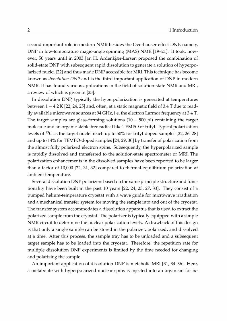
4.4. Results . . . . . . . . . . . . . . . . . . . . . . . . . . . . . . . . . . . . . 984.4.1. DNP-CP using AHP . . . . . . . . . . . . . . . . . . . . . . . . . 984.4.2. Dissolution DNP-CP . . . . . . . . . . . . . . . . . . . . . . . . . 99

Contents vii
4.4.3. Multiple-contact time DNP-CP . . . . . . . . . . . . . . . . . . . 1014.5. Discussion . . . . . . . . . . . . . . . . . . . . . . . . . . . . . . . . . . . 103
5. A spin-thermodynamic model of thermal mixing 1055.1. Model description . . . . . . . . . . . . . . . . . . . . . . . . . . . . . . . 1055.2. Solution of the differential equations and model fitting . . . . . . . . . 1085.3. Results and Discussion . . . . . . . . . . . . . . . . . . . . . . . . . . . . 109
6. The influence of sample parameters on dissolution DNP 1176.1. Pyruvate/trityl-based samples . . . . . . . . . . . . . . . . . . . . . . . 117
6.1.1. Solid-state DNP and T1 . . . . . . . . . . . . . . . . . . . . . . . 1176.1.2. Liquid-state T1 dependence on pH . . . . . . . . . . . . . . . . . 1186.1.3. Results and discussion . . . . . . . . . . . . . . . . . . . . . . . . 118
6.2. TEMPO-based samples . . . . . . . . . . . . . . . . . . . . . . . . . . . . 1226.2.1. Solid-state DNP enhancement . . . . . . . . . . . . . . . . . . . 1226.2.2. CP efficiency . . . . . . . . . . . . . . . . . . . . . . . . . . . . . 1236.2.3. Dissolution efficiency . . . . . . . . . . . . . . . . . . . . . . . . 1236.2.4. Results and discussion . . . . . . . . . . . . . . . . . . . . . . . . 123
Conclusion 129
Outlook 133
Appendices 137
A. Cryogenic heat flow 139A.1. Heat flow through a succession of materials . . . . . . . . . . . . . . . . 143
B. Cavity dimensions 145
Bibliography 149
Acknowledgement 161
Curriculum Vitae 163
List of Publications 165


Abbreviations and Symbols
b Inverse spin temperatureDwe EPR line widthe Polarization enhancementg Gyromagnetic ratiokB Boltzmann constantT1 Spin-lattice relaxation time, longitudinal relaxation timeT2 Spin-spin relaxation time, transverse relaxation timeT1,r Rotating-frame relaxation timeTTM Thermal mixing time1D One dimensionalH Hamilton operatorAHP Adiabatic half-passageCE Cross effectCL Cooling reservoirCP Cross polarizationcw Continuous waveCZ Carbon Zeeman reservoirDNP Dynamic nuclear polarizationDNP-CP Dynamic nuclear polarization in combination with cross polar-
izationDQ Double quantumEPR Electron paramagnetic resonanceFWHM Full width at half maximumhfi Hyperfine interactionHZ Proton Zeeman reservoirif Interaction frameL Lattice
ix

x Abbreviations and Symbols
LOD Longitudinal detected (EPR)MRI Magnetic resonance imagingMRS Magnetic resonance spectroscopymw MicrowaveNMR Nuclear magnetic resonanceNZ non-Zeeman reservoirOE Overhauser effectPTFE Polytetrafluorethylenrf Radio frequencySE Solid effectSL Spin lockSNR Signal-to-noise ratioTM Thermal mixingVI Virtual instrumentZQ Zero quantum

List of substances
The substances used and mentioned in this work have been acquired from:
• [1-13C]pyruvic acid ("pyruvate"): ISOTEC/Sigma Aldrich
• [13C]urea: ISOTEC/Sigma Aldrich
• [1,4-13C]fumaric acid: Sigma Aldrich
• TEMPO: 2,2,6,6-tetramethyl-1-piperidinyloxy, Sigma Aldrich
• trityl: tris (8-carboxyl-2,2,6,6-tetra(2-(1-hydroxyethyl))-benzo[1,2-d;4,5-d’] bis (1,3)dithiole-4-yl) methyl sodium salt, donation
• Glycerol-d3: exchangeable protons of glycerol deuterated in LPC, ETH (by Fa-bienne Arn and Guido Grassi)
• Glycerol-d8: donated by EPR group ETH, Prof. Gunnar Jeschke
• DMSO-d6: Cambridge Isotopes
• D2O: Cambridge Isotopes
• Gd: Gadovist, Bayer HealthCare
xi


Abstract
An important limitation of nuclear magnetic resonance (NMR) applications is thelow intrinsic sensitivity that can be overcome by hyperpolarization techniques suchas dynamic nuclear polarization (DNP). Ardenkjær-Larsen et al. extended the estab-lished solid-state DNP method in 2003 by subsequent dissolution of the hyperpolar-ized sample (dissolution DNP) making it applicable to in-vivo magnetic resonanceimagining (MRI) and spectroscopy (MRS).
The common DNP polarization protocol used in combination with the publishedsingle-sample polarizers allows only low dissolution repetition rates, limited to lessthan one dissolution experiment per hour. Decreasing the minimum repetition timebetween successive dissolution DNP experiments could not only ease the screeningof sample parameters in multi-sample studies, but could allow DNP enhanced MRSexperiments that demand a fast succession of injections of hyperpolarized substances.
To increase the repetition rate of dissolution DNP experiments, two approaches arebeing investigated in this thesis: a) the simultaneous polarization of multiple samplesfollowed by successive dissolutions in a multi-sample dissolution DNP system, andb) the combination of dissolution DNP with Hartmann-Hahn cross polarization (CP)allowing fast polarization of 1H followed by polarization transfer from 1H to 13Cnuclei.
In the Instrumentation section, the design and performance results of a home-builtcryogenic DNP setup are presented with two compatible DNP probes. The first probeis a single-sample probe that allows static heteronuclear solid-state NMR experimentswith high sensitivity and radio frequency (rf) field strengths up to 100 kHz. The sec-ond probe is a dissolution DNP probe with multi-sample functionality. A revolver-style sample changer accommodating up to six samples allows to exchange the sam-ples between different positions during cryogenic operation. A resonant microwavecavity is used to increase the DNP efficiency at low incident microwave power, andNMR and EPR capabilities are included in the polarizer to monitor and characterize
xiii

xiv Abstract
the DNP process.The multi-sample probe has been found to be highly convenient to conduct series
of solid-state DNP experiments with varying sample compositions, since the time-consuming changing of samples in and out of the cold space can be avoided. Al-though simultaneous polarization of all samples is possible, the multi-sample probedoes not allow fast-sequential dissolution DNP experiments in the current setup,since the dissolution of one sample depletes the polarization of the remaining sam-ples.
Using the single-sample probe, the combination of DNP with CP (DNP-CP) wasinvestigated with the aim to reduce the polarization build-up time on 13C. Thisapproach is based on the fact that the polarization time on high-g nuclei, such as1H, is usually shorter than that of low-g nuclei, such as 13C. A modification of theHartmann-Hahn CP is presented using adiabatic half-passage pulses. It allows moreefficient polarization transfer at low rf-field strengths, which is especially importantin the combination with dissolution DNP probes since these usually suffer from alimited rf-field strength. Important aspects for the combination of dissolution DNPwith CP are discussed and the DNP-CP experiment is further improved by applyingmultiple-contact time CP to a suitable sample.
To combine DNP-CP with subsequent dissolution, an additional NMR circuit is in-corporated into the dissolution probe allowing heteronuclear NMR experiments withfield strengths up to 30 kHz. It is shown, that the polarization transfer gained by theCP in the solid state is retained during the dissolution process. With this technique,the polarization is accelerated by a factor larger than two while enhancing the finalpolarization level.
To gain further insight into the dynamics during heteronuclear DNP experiments,a spin-thermodynamic model is applied. It models the dynamics of the 1H and 13Cpolarization levels during heteronuclear DNP experiments for various initial condi-tions of the nuclear polarizations. Finally, the influences of radical concentration andsample pH on the dissolution DNP-CP efficiency are investigated.
In conclusion, this thesis provides technical, methodological, and experimentalcontributions to the advancement of the dissolution DNP technique, amongst oth-ers, towards faster repetition rates. Along the way, it provides the research field ofNMR and MRI at the ETH with a readily available tool for generating hyperpolarizednuclear spins in solution.

Zusammenfassung
Den grösste Nachteil der Kernmagnetresonanz (NMR) stellt deren geringe Sensitivi-tät dar. Diese kann in bestimmten Anwendungen durch Hyperpolarisationsmetho-den wie Dynamic Nuclear Polarization (DNP) verbessert werden. Ardenkær-Larsenhat 2003 gezeigt, dass sich DNP in Festkörpern durch schnelles Auflösen der hyper-polarisierten Substanz für die Magnetresonanz Tomographie (MRT) und Spektrosko-pie (MRS) nutzbar machen lässt (Dissolution DNP).
Die seit 2003 vorgestellten Einzel-Proben-DNP-Systeme und die darin angewand-ten Polarisationsprotokolle erlauben nur geringe Wiederholungsraten aufeinander-folgender Dissolution-DNP-Experimente. Eine Reduktion der Repetitionszeit könntesowohl das Messen von Probenreihen beschleunigen, als auch MRS Studien ermögli-chen, die eine schnelle Abfolge aufeinanderfolgender Applikationen hyperpolarisier-ter Substanzen voraussetzen.
Um die Repetitionszeit zu verkürzen, werden in dieser Dissertation zwei Ansät-ze verfolgt: das gleichzeitige Polarisieren mehrerer Proben sowie die Erweiterungdes Dissolution-DNP-Experiments durch Hartmann-Hahn-Kreuzpolarisation (CP),die das schnellere Hyperpolarisieren von 1H Kernen ausnutzt und anschliessend de-ren Polarisierung auf die 13C Kerne überträgt.
Zunächst werden das Design und die Leistungsmerkmale eines Tieftemperatur-DNP Systems vorgestellt sowie zwei dafür entwickelte DNP-Probenköpfe. Der ersteProbenkopf ist ein statischer Tieftemperatur-NMR-Probenkopf, der für Multikern-NMR-Experimente mit hohen Radiofrequenz (RF)-Feldstärken bis zu 100 kHz op-timiert ist. Der zweite Probenkopf fasst bis zu 6 Proben und ist mit einer Auflöse-vorrichtung ausgestattet. Das revolverartige Skelett des Probenkopfes erlaubt es, dieProben bei allen erreichbaren Temperaturen innerhalb des Probenkopfes zu wech-seln. Ein Mikrowellenresonator ermöglicht dabei bei reduzierter Mikrowellenleist-ung einen effizienten Hyperpolarizationsprozess, der durch Detektionsmöglichkei-ten der EPR und NMR untersucht werden kann.
xv

xvi Zusammenfassung
Der Probenkopf mit Revolvermechanismus erleichtert das Messen der DNP-Ef-fizienz von Probenreihen, da hierbei das zeitaufwändige Wechseln der Proben vomkalten in den warmen Bereich vermieden werden kann. Trotz der Fähigkeit, bis zu6 Proben gleichzeitig zu polarisieren, ermöglicht der Probenkopf derzeit allerdingsnicht die schnelle Abfolge von Dissolution-DNP-Experimenten, da das Auflösen ei-ner Probe die Polarisierung der verbleibenden Proben bedeutend schwächt.
Mittels des Probenkopfes für Multikern-NMR-Experimente wurde die Kombina-tion von DNP mit CP (DNP-CP) erprobt, mit dem Ziel, die Polarisationsdauer der13C Kerne zu reduzieren. Dieser Ansatz nutzt die meist schnellere Polarisation vonKernen mit hohem gyromagnetischem Verhältnis g, etwa 1H, im Vergleich zur Pola-risation von Kernen mit kleinem g, etwa 13C. Eine Modifikation des klassischen CPdurch die Verwendung adiabatischer Pulse wird vorgestellt, durch die die Effizienzdes CP bei niedrigen RF-Feldstärken gesteigert werden kann. Dies ist wichtig bei derAnwendung von CP in Dissolution-DNP-Probenköpfen, die meist nur geringe RF-Feldstärken zulassen. Weitere Aspekte des DNP-CP-Experiments mit Hinblick aufdie Kombination mit anschliessender Auflösung werden diskutiert und die Effizienzdes Experiments wird durch wiederholtes Anwenden des CP gesteigert.
Die Kombination von DNP-CP mit anschliessender Auflösung wird mittels einerErweiterung des Probenkopfes mit Auflösevorrichtung demonstriert, durch die Mul-tikern-NMR-Experimente bis zu 30 kHz RF Feldstärke möglich sind. Es wird gezeigt,dass der im Festkörper erreichte Polarisationstransfer durch den Auflösevorgang indie flüssigen Phase übertragbar ist. Dadurch wird die effektive Polarisationsrate der13C Kerne mehr als verdoppelt bei gleichzeitiger Verstärkung des erreichten Polari-sationsgrades.
Um die Dynamik der Kernpolarisationen während Multikern-DNP-Experimentenzu untersuchen, wird ein Modell basierend auf der Spin-Thermodynamik angewandt.Das vorgestellte Modell erlaubt es, die Dynamik der 1H und 13C Kernpolarisationennach verschiedenen experimentellen Anfangspräparationen vorherzusagen. Zusätz-lich wird die Effizienz des Dissolution-DNP-CP-Experiments in Abhängigkeit derKonzentration der Radikale sowie des pH-Wertes untersucht.
Zusammenfassend leistet diese Dissertation Beiträge zur technischen und metho-dologischen Weiterentwicklung der Dissolution-DNP-Methode mit Fokus auf der Be-schleunigung der möglichen Wiederholungsrate. Zusätzlich stellt der entwickelte ex-perimentelle Aufbau dem NMR- und MRI-Forschungsfeld der ETH Zürich ein Tool

xvii
zur Hyperpolarisation von Kernspins zur Verfügung.


1. Introduction
The inherently low sensitivity is a major drawback of nuclear magnetic resonance(NMR) and magnetic resonance imaging (MRI) and leads to long measurement times.This is a problem, for example, in spatially-resolved magnetic resonance spectroscopy(MRS), where the distribution of metabolic substances in an organism is of interest.The large background of abundant water protons overwhelms the 1H resonances ofpotentially interesting substrates in low endogenous concentrations. Magneticallyactive isotopes other than 1H, e.g., 15N or 13C are difficult to detect with sufficientspatial resolution due to their low natural abundance and lower gyromagnetic ratiog.
Besides increasing the static magnetic field or lowering the temperatures (the so-called brute-force method), various methods have been proposed over the years to in-crease the nuclear spin polarization over the thermal equilibrium. Such hyperpolar-ization techniques include optical pumping of noble gases [1–3], para-hydrogen inducedpolarization [4, 5], the Haupt effect in methyl groups [6–8], chemically-induced dynamicnuclear polarization [9], and dynamic nuclear polarization using free radicals (DNP) [10].
In DNP, electron polarization is transferred to the nuclei under microwave irra-diation of the electron spins. After the first prediction of the effect in metals byOverhauser in 1953 [11] and the experimental verification of this Overhauser effect byCarver and Slichter shortly after [12], experimental and theoretical research on DNPstarted prospering: Jeffries proposed a similar DNP effect in non-conducting solidsat low temperatures [13], which was first demonstrated and named as the solid effectby Abragam and Proctor in 1958 [14]. The theoretical description of the DNP mecha-nisms have been extended to systems with abundant radicals with large line widthsby the work of Provotorov [15], Borgini [16], and Abragam and Goldman [10] in the1960s and 1970s leading to the description of DNP via thermal mixing.
In 1967, Hwang and Hill observed the so-called cross effect [17, 18]. Together withthe developments by Wind and Griffin in the 1980s and 1990s this effect led DNP to its
1
2 1 Introduction
second important role in modern NMR besides the Overhauser effect DNP, namely,DNP in low-temperature magic-angle spinning (MAS) NMR [19–21]. It took, how-ever, 50 years until in 2003 Jan H. Ardenkjær-Larsen proposed the combination ofsolid-state DNP with subsequent rapid dissolution to generate a solution of hyperpo-larized nuclei [22] and thus made DNP accessible for MRI. This technique has becomeknown as dissolution DNP and is the third important application of DNP in modernNMR. It has found various applications in the field of solution-state NMR and MRI,a review of which is given in [23].
In dissolution DNP, typically the hyperpolarization is generated at temperaturesbetween 1� 4.2 K [22, 24, 25] and, often, at a static magnetic field of 3.4 T due to read-ily available microwave sources at 94 GHz, i.e, the electron Larmor frequency at 3.4 T.The target samples are glass-forming solutions (10 � 500 µl) containing the targetmolecule and an organic stable free radical like TEMPO or trityl. Typical polarizationlevels of 13C as the target nuclei reach up to 50% for trityl-doped samples [22, 26–28]and up to 14% for TEMPO-doped samples [24, 29, 30] by transfer of polarization fromthe almost fully polarized electron spins. Subsequently, the hyperpolarized sampleis rapidly dissolved and transferred to the solution-state spectrometer or MRI. Thepolarization enhancements in the dissolved samples have been reported to be largerthan a factor of 10,000 [22, 31, 32] compared to thermal-equilibrium polarization atambient temperature.
Several dissolution DNP polarizers based on the same principle structure and func-tionality have been built in the past 10 years [22, 24, 25, 27, 33]. They consist of apumped helium-temperature cryostat with a wave guide for microwave irradiationand a mechanical transfer system for moving the sample into and out of the cryostat.The transfer system accommodates a dissolution apparatus that is used to extract thepolarized sample from the cryostat. The polarizer is typically equipped with a simpleNMR circuit to determine the nuclear polarization levels. A drawback of this designis that only a single sample can be stored in the polarizer, polarized, and dissolvedat a time. After this process, the sample tray has to be unloaded and a subsequenttarget sample has to be loaded into the cryostat. Therefore, the repetition rate formultiple dissolution DNP experiments is limited by the time needed for changingand polarizing the sample.
An important application of dissolution DNP is metabolic MRI [31, 34–36]. Here,a metabolite with hyperpolarized nuclear spins is injected into an organism for in-

3
vivo tracing of the marker molecule and its metabolic products. This procedure opensunprecedented opportunities in MRI. Like most hyperpolarization techniques, thedissolution DNP method is limited by the fact that the high polarization is availableonly for a time window on the order of T1. Consequently, the technique is restrictedto the detection of hyperpolarized low-g nuclei, which usually have longer relaxationtimes than high-g nuclei. It is found, that the polarization transfer from electrons tolow-g nuclei like 13C is usually slow and requires polarization times often exceeding1 hour. Therefore, the repetition time for multiple dissolution DNP experiments usingsingle-sample polarizers is limited to > 1 hour [22, 30].
Decreasing the minimum repetition time between successive dissolution DNP ex-periments can be important for, e.g., cardiac experiments of repeated ischemia /reperfusion to study conditioning of the heart. Furthermore, the investigation ofthe dependence of the DNP efficiency on various sample parameters requires serialexperiments, which could be simplified by having multiple samples loaded in thepolarizer simultaneously.
It has been shown in the past that the combination of DNP to 1H and Hartmann-Hahn cross polarization (CP) [37] to 13C is a possible way to speed up the DNPprocess and enhance the polarization of low-g nuclei under MAS DNP conditions[20, 38, 39]. Under conditions similar to the ones in dissolution DNP experiments,however, the combination of DNP with CP has not been presented before this work.The obstacles to overcome when realizing such experiments arise mainly from theNMR circuits of dissolution DNP setups with a single radio-frequency channel andrelatively low radio frequency (rf) amplitudes available.
It is the target of this thesis to contribute to technical and methodological develop-ments towards dissolution DNP experiments with an increased repetition rate com-pared to the rates achievable by the published dissolution DNP systems. This goal isapproached from two sites: on the one hand a multi-sample dissolution DNP probehas been developed to investigate the possibility of simultaneous polarization of mul-tiple samples and successive dissolutions. On the other hand, the combination of dis-solution DNP with a modification of the Hartmann-Hahn CP method is presented,which exploits the fast polarization build up of 1H in combination with subsequentpolarization transfer from 1H to 13C to decrease the overall build-up time of the 13Cpolarization.
In chapter 2, the theoretical framework used in this work is introduced and a dis-

4 1 Introduction
cussion is given, helping to answer the question which DNP mechanism is dominantin the experimental data presented. The developed instrumentation is presentedin chapter 3 and performance results of the dissolution DNP system are given. Inchapter 4, the combination of dissolution DNP and CP is introduced. Peculiaritiesof this experiment are discussed, a modification of the cross polarization techniqueis presented exploiting adiabatic half-passage rf pulses, and the first solution-stateresults are presented that have been achieved with this method. In chapter 5, a spin-thermodynamic model is applied to experimental data to gain insight into the dy-namics during heteronuclear DNP experiments. Finally, in chapter 6, the influenceof selected sample parameters on the efficiency of dissolution DNP experiments ispresented.

2. Theoretical background
2.1. Magnetic Resonance
The prerequisite of each DNP mechanism is the interaction of electron spins withnuclear spins in an external magnetic field. The scientific discipline describing nu-clear spins and electron spins in magnetic fields is called Magnetic Resonance (MR).Numerous text books offer comprehensive overviews and in-depth theoretical treat-ments, such as [40–43]. The quantities which are most important for the theoreticaltreatment of DNP will be introduced in the following.
2.1.1. Hamiltonians in NMR and EPR
In the laboratory frame of reference the Hamiltonian of a system of interacting electron-nuclear spins can be written as
H lab = He,Z + Hn,Z + Hh f i + Hee + Hnn + Hmw + Hr f (2.1)
precluding electron spin systems forming group spins with S > 1/2. The interactionsare:
electron Zeeman: He,Z
nuclear Zeeman: Hn,Z
electron-nuclear hyperfine: Hh f i
weak electron-electron: Hee
nuclear-nuclear: Hnn
microwave irradiation: Hmw
radio frequency irradiation: Hr f .
(2.2)
Above, as well as in the following, S and I always stands for the electron and nu-
5

6 2 Theoretical background
clear spin operators, respectively. In the product base, their order will be S I. AllHamiltonians will be given in angular frequency units throughout this work. Thisimplies that, e.g. the spin operator Iz for a spin-1/2 is written as:
Iz =12
1 00 �1
!
and that the energy of a spin system in Joules is calculated via:
E = hhH i.
Interaction-frame representation
It is a common tool of MR to describe the state of a spin systems and its evolution inthe interaction frame with respect to the interaction Hi f . Any operator O is representedin this interaction frame via the transformation:
O0 = eiHi f tOe�iHi f t. (2.3)
It is common practice to truncate the interaction frame Hamiltonians to their sec-ular (time independent) contributions, while dropping the non-secular (time depen-dent) contributions. This can be justified by averaging the Hamiltonian over a timelarger than the periodicity of the non-secular contributions and should be accountedfor by, e.g., an overbar on the Hamiltonian. The latter is usually omitted and in re-turn it is noted that the Hamiltonian is truncated to the secular contributions. Thisinteraction-frame transformation and secular truncation allows a simplification of theHamiltonians and will be used frequently throughout this work.
Electron Zeeman interaction
If electrons are included in the spin system, the electron Zeeman interaction is theleading term, expressed as
He,Z = Âi
µBh~BT
0 giSi (2.4)

2.1 Magnetic Resonance 7
or with ~BT0 = (0, 0, B0)
He,Z = Âi
µBh
B0
⇣
gizxSi
x + gizySi
y + gizzSi
z
⌘
(2.5)
with the Bohr magneton µB, the transposed external magnetic field vector ~BT0 , and
the g-tensor gi of each electron i. For simplicity of subsequent theoretical discussions,the high-field approximation can be applied leaving only the z-component. Conse-quently, the Zeeman Hamiltonian of electron i can be rewritten as:
H ie,Z = weS
iz + Di Si
z (2.6)
with we = µBh giso B0 and Di = wi � we = µB
h B0(gizz � giso). Equation 2.6 implies
the restriction that all electrons have the same isotropic g-value giso and only differ intheir relative orientation to the z-axis. This simplification is reasonable for the systemswith only a single free radical species present.
The Zeeman Hamiltonian in equation 2.6 reveals an on-resonance (first term) andoff-resonance term. The resonance frequency of an electron will thus depend on itsrelative orientation of the g-tensor to the magnetic field (and therefore to the lab-oratory coordinate system). The relative spread of frequencies arising from this g-anisotropy strongly depends on the radical chosen and is in the order of 2.75 ⇥ 10�4
for the trityl radical and 3.6 ⇥ 10�3 for the TEMPO radical used in this work.
Finally, in the electron Zeeman interaction frame with Hi f = weSiz equation 2.6
reduces to its off-resonant term:
H ie,Z = Di Si
z. (2.7)
Nuclear Zeeman interaction
The second important interaction (even though in general not larger than the hy-perfine interaction) is the interaction of the nuclear spins with the external magneticfield:
Hn,Z = �Âj
gj~BT0 Ij = Â
jw
jn Ij
z (2.8)

8 2 Theoretical background
assuming that ~BT0 = (0, 0, B0), with the nuclear Larmor frequency w
jn = �gjB0 and the
nuclear gyromagnetic ration gj of the nuclear spin j. In this work, only chemicallyequivalent nuclei will be treated, so that chemical shift contributions can be neglected.
Electron-nuclear hyperfine interaction
The most important interaction for DNP is the electron-nuclear hyperfine interaction
Hh f i = Âj,i
SiAIj (2.9)
where A is the hyperfine interaction tensor. This tensor contains an isotropic (or Fermicontact) part as well as anisotropic components arising from electron-nuclear dipolarcouplings [43, ch. 3.1.3]. The hyperfine Hamiltonian can thus be separated into
Hh f i = H isoh f i + H aniso
h f i (2.10)
with
H isoh f i = Â
i,jai,jSiIj (2.11)
H anisoh f i = Â
i,j
µ04p
gegnhr3
i,j(Ai,j + Bi,j + Ci,j + Di,j + Ei,j + Fi,j) (2.12)

2.1 Magnetic Resonance 9
with ge ⌘ µBh g and the Fermi-contact interaction strength ai,j (see [43]). The so called
dipolar alphabet is given by
Ai,j = Siz Ij
z
⇣
1 � 3 cos2 qi,j
⌘
Bi,j =⇣
S+i I�j + S�i I+j⌘ 3 cos2 qi,j � 1
4
Ci,j =⇣
S+i Ijz + Si
z I+j⌘ �3 sin qi,j cos qi,je�ifi,j
2
Di,j =⇣
S�i Ijz + Si
z I�j⌘ �3 sin qi,j cos qi,je�ifi,j
2
Ei,j = S+i I+j�3 sin2 qi,je�i2fi,j
4
Fi,j = S�i I�j�3 sin2 qi,jei2fi,j
4.
(2.13)
Above, ri,j, qi,j, and fi,j are the spherical coordinates of the vector connecting the elec-tron i with the coupled nucleus j. The anisotropic hyperfine interaction is caused bydipolar coupling of the electron and nuclear magnetic moments through space. Theisotropic part arises from a non-zero overlap of probability density of the electron andthe nucleus. It is therefore restricted to intramolecular interactions and to electronswith wave functions (at least partially) in the s-orbital.
Electron-electron and nuclear-nuclear interactions
Both, pairs of close-by electrons and pairs of close-by nuclei interact via the dipolarcoupling of their magnetic moments. This coupling has the same formal shape as theanisotropic hyperfine interaction given in equation 2.12 using the dipolar alphabetgiven in equation 2.13.
In the case of the electron-electron interaction, this holds true only for weakly cou-pled electron pairs without orbital overlap [43, ch. 3.1.6]. It is justified to makethis simplification here since in this work only radical dopants are considered with asingle unpaired electron. Otherwise, the zero-field splitting and the exchange couplingwould have to be taken into account.
In the high-field approximation, one can transform into the interaction frames ofthe Zeeman interactions. In this case, both for electron-electron dipolar interactions

10 2 Theoretical background
and homonuclear dipolar interactions equation 2.12 reduces to its secular term andis truncated after the term Bi,j. For heteronuclear interactions one can transform intoa double rotating frame with both Zeeman interactions. In this case equation 2.12simplifies even further by truncation after the term Ai,j (as will be used in section2.3.1).
For nuclear-nuclear interactions additionally an isotropic interaction exists calledJ-coupling or scalar coupling. Since it is usually several orders of magnitude smallerthan the dipolar coupling it is only observed in liquids or in MAS-NMR where thedipolar couplings are averaged out. Therfore it will be neglected in this work.
Microwave and radio-frequency irradiations
The manipulation of the spin system is achieved by applying microwave (mw) irra-diation with a frequency close to the electron Zeeman resonance or radio-frequency(rf) irradiation close to the nuclear Larmor frequency.
The mw irradiation is usually introduced to the sample via a wave guide whilethe rf irradiation is generated by a resonating coil surrounding or in the vicinity ofthe sample. In both cases, the Hamiltonian can be written in analogy to the ZeemanHamiltonian, e.g. for the case of rf irradiation
Hr f = �Âj
gjn~B1Ij (2.14)
with the magnetic component ~B1 of the generated electromagnetic field. The trans-verse component of the rf-field with field strength B1 can be written as
(~B1)? = 2B1 cos(wr f t + f)~ex (2.15)
arbitrarily aligning it with the x-axis of the laboratory frame and allowing for a phasef.
The longitudinal component (~B1)k is usually several orders of magnitude smallerthan B0 and can be neglected. Thus (~B1)? = ~B1 and the Hamiltonians for rf and mw

2.1 Magnetic Resonance 11
irradiation read:
Hr f = Âj�g
jn2Br f
1 cos(wr f t + f) Ijx (2.16)
Hmw = Âi�gi
e2Bmw1 cos(wmwt + j) Si
x. (2.17)
In the interaction frames with respect to the Zeeman interactions the rf and mwHamiltonians become (for single spins)
Hr f = �gn2Br f1
12�
cos((wr f � wn,i f )t + f) + cos((wr f + wn,i f )t + f)�
Ix
Hmw = �ge2Bmw1
�
cos((wmw � we,i f )t + j) + cos((wmw + we,i f )t + j)�
Sx
and if the interaction frame frequencies are chosen equal to the irradiation frequencies(wr f = wn,i f , wmw = we,i f ) reduce further to
Hr f = �gnBr f1 Ix � gnBr f
1 cos(2wr f t) Ix
Hmw = �geBmw1 Sx � geBmw
1 cos(2wmwt) Sx
where j = f = 0 can be defined without losing generality.
If the secular truncation is applied to the interaction-frame irradiation Hamiltoni-ans they finally simplify to
Hr f = w1,n Ix (2.18)
Hmw = w1,e Sx (2.19)
with the nutation frequencies w1,n = �gnBr f1 and w1,e = �geBmw
1 .
2.1.2. Spin ensembles and the density operator
Macroscopic systems with N � 1 spins are treated as "ensembles". If the quantummechanical state of each spin i is written as function of the eigenbase of the Iz operator|ai and |bi as
|yi = c1|ai+ c2|bi (2.20)

12 2 Theoretical background
then the expectation value of any spin operator is a function of the product of thecoefficients cic⇤j . For an ensemble of equivalent spins, the expectation value can bederived from the expectation value of the isolated spin by averaging over all N prod-ucts cic⇤j , therefore the knowledge of cic⇤j for all four combinations of i, j = 1, 2 issufficient to fully characterize the spin system with respect to the spin observables.This motivates the definition of the density operator
r ⌘ |yihy|
which becomes
r =
c1c⇤1 c1c⇤2c2c⇤1 c2c⇤2
!
(2.21)
if written as matrix in the eigenbase of Iz. The density matrix is composed by theproducts of coefficients and it can be shown that the density operator fully character-izes the state of a system. The overbar will be dropped from this point on.
The diagonal entries of the spin density operator 2.21 are called populations of state i(cic⇤i ) while the off-diagonal entries are called coherences. If the spin system is at equi-librium with the surrounding lattice the density operator is diagonal (in the eigenbaseof the Hamiltonian) with a Boltzmann distribution of populations:
r =1
Trn
e�bhHo e�bhH (2.22)
whereb =
1kBT
(2.23)
defines the inverse spin temperature b using the usual terminology (e.g. [10, p. 401])and kB is the Boltzmann constant (for more information see section 2.2.3.1). At ther-mal equilibrium the spin temperature becomes equal to the lattice temperature T =
TL.
To reach equilibrium after a perturbation the coherences decay with the phenomeno-logical time constant T2 (spin-spin relaxation time) while the populations approachthere equilibrium distribution with the time constant T1 (spin-lattice relaxation time).

2.1 Magnetic Resonance 13
2.1.3. Sensitivity in NMR
The detection of nuclear resonances is usually achieved by observing induced volt-ages in the NMR coil. If the coil axis is assumed to be aligned with the x-axis of thecoordinate system, then the induced signal strength S is proportional to the magneti-zation along x:
S µ Mx ⌘ gnNhIxi µ c1c⇤2 + c2c⇤1
using the relation hOi = Tr�
r O
. As shown in the preceding section the coherencesare zero in thermal equilibrium. Therefore, before detection rf pulses are used togenerate detectable coherences. In the Zeeman interaction frame one can assume therf-pulse to rotate the density operator around the y-axis (with Hr f analog to equation2.18 with Iy instead of Ix) such that
r(t) = e�iHr f tr(0)eiHr f t =
cos w12 t � sin w1
2 t
sin w12 t cos w1
2 t
!
c01c0⇤
1 00 c0
2c0⇤2
!
cos w12 t sin w1
2 t
� sin w12 t cos w1
2 t
!
=
c01c0⇤
1 cos2 w12 t + c0
2c0⇤2 sin2 w1
2 t (c01c0⇤
1 � c02c0⇤
2 ) sin w12 t cos w1
2 t
(c01c0⇤
1 � c02c0⇤
2 ) sin w12 t cos w1
2 t c01c0⇤
1 sin2 w12 t + c0
2c0⇤2 cos2 w1
2 t
!
.
The signal strength after the pulse is thus
S µ 2(c01c0⇤
1 � c02c0⇤
2 ) sinw12
t cosw12
t
and becomes maximum for a 90� pulse (w1t = 90�):
S µ (c01c0⇤
1 � c02c0⇤
2 ).
The difference in populations prior to the pulse is therefore determining the signalintensity in NMR experiments. It is called
Polarization P ⌘ (c1c⇤1 � c2c⇤2) (2.24)
and it is the target of DNP to enhance its value above thermal equilibrium.
Corresponding to equation 2.22 the polarization of a spin-1/2 system (with g > 0)

14 2 Theoretical background
reads at thermal equilibrium:
P =ebLh w
2 � e�bLh w2
ebLh w2 + e�bLh w
2= tanh
⇣
bLhw
2
⌘
(2.25)
if the Zeeman interaction (equation 2.8) is the dominant contribution to the Hamilto-nian. In the high-temperature approximation, where bLhw ⌧ 1 this can be simplifiedby truncating after the linear term of the series expansion:
P ⇡ bLhw
2. (2.26)
In the context of this work, the usage of the high-temperature approximation hasto be handled with care since temperatures as low as 1.3 K are reached. For 13Cand 1H at 1.3 K the exact polarization levels are 0.07% and 0.29%, respectively (atthe given field of 3.35 T). Therefore, the relative errors made for the nuclei using thehigh-temperature approximation is negligible. For electrons, however, the relativeerror rises above 1% around 13 K and reaches ⇠ 9% at 4.2 K.

2.2 Dynamic Nuclear Polarization 15
2.2. Dynamic Nuclear Polarization
2.2.1. The mechanisms of DNP
Since Overhauser suggested in 1953 [11] to enhance the nuclear polarization of met-als by saturating their EPR line several similar mechanisms have been proposed allutilizing microwave irradiation. They are today summarized as DNP methods. Thepurpose of this section is to introduce the different DNP mechanisms and to empha-size their differences and circumstances under which they occur with a treatmentsimilar to [19].
While the hyperfine term in equation 2.1 is important for all DNP mechanisms,the electron-electron interactions are relevant for the thermal mixing DNP, which willbe introduced later. They can be described in analogy to the anisotropic part of thehyperfine interaction (equation 2.12, with ge and S substituted for gn and I). Animportant consequence of these interactions is the electron-electron cross relaxation,mediated by the term Bi,j. Another result of Hee is dipolar broadening of the EPRline, referred to as homogenous broadening [43, ch. 3.3.1].
Another reason for EPR line broadening can be a spread of Larmor frequencies wie
of independent electron spins, called inhomogenous broadening. The reason for thiscan be, among others [43, ch. 3.3.2], g-anisotropy or hyperfine interactions to nucleiat different relative electron-nuclear positions. The EPR line width due to both ho-mogenous and inhomogenous broadening will be denoted as Dwe in the following.
The dominating DNP mechanisms, depending mainly on the time dependence ofthe contributions to the overall Hamiltonian in equation 2.1, are:
i) The Overhauser effect (OE) relies on cross relaxation between coupled electron-nucleus pairs while saturating the electron Zeeman transition. For the cross re-laxation to occur, Hh f i has to be time-dependent on a scale similar to w�1
e [19].The OE thus is characteristic for metals (such as Li, in which Carver and Slichterinitially demonstrated the OE [12]) or liquids doped with paramagnetic com-pounds, as was first shown by Abragam in 1955 [44]. In solids with fixed para-magnetic centers the OE therefore does not occur. A theoretical treatment of thiseffect can be found in [45, 46] or in the reviews [47, 48].
ii) The Solid (state) Effect (SE) occurs when the time-average value of H anisoh f i is non-

16 2 Theoretical background
zero, i.e., if there are no modulations averaging the anisotropic hyperfine inter-actions to zero. Furthermore, the EPR line has to be narrow compared to the nu-clear Larmor frequency, i.e., wn > Dwe where Dwe denotes the EPR line width.This restricts the system to non-conducting solids with fixed paramagnetic cen-ters at low concentrations and low g-anisotropy. The SE was proposed by Jeffriesin 1957 [13] and first demonstrated and named by Abragam and Proctor in 1958[14]. A comprehensive review can be found in [49] and in-depth quantum me-chanical treatments are given by the group of Robert Griffin [50] and ShimonVega [51–53].
iii) The Cross Effect (CE) can occur under the same experimental conditions as theSE. However, it is a three-spin {e-e-n} process in which two electrons with
|we,1 � we,2| ⇡ wn
perform a flip-flop and the nucleus flips by taking up the remaining energy. Thisrestricts the effect to solids with an inhomogenous EPR line width Dwe > wn. TheCE was first observed by Hwang and Hill [17, 18] and is nowadays the predom-inant mechanism used in high-field 100 K DNP-MAS experiments. For these,bi-radicals or mixtures of radicals are used rather than mono-radicals so that thechance of finding an electron pair matching the CE condition is larger [54, 55]. Areview on the CE with focus on high magnetic fields is given by Hu [56] and aquantum mechanical treatment can be found in [57].
iv) The Thermal Mixing (TM) effect also occurs if the time-average of H anisoh f i is zero
and if Dwe > wn. In contrast to the CE it can occur even at large electron concen-trations so that the inhomogenously broadened EPR line becomes additionally(partly) homogenously broadened. Most important, for the TM the CE condi-tion can be met not only by the irradiated electron spin packet but by any arbitraryelectron-electron pair. The TM effect is explained by the spin-temperature theorydeveloped by Redfield, Provotorov, Abragam, and others [10, 15, 16, 58, 59] andis understood to be the major mechanism in dissolution DNP experiments.
The experiments presented later in this work utilize DNP at mainly 1.3 to 4.2 Kin amorphous organic solids doped with stable radicals in the range of several tensof mM. For these conditions the above discussion points out that SE, CE, and TM

2.2 Dynamic Nuclear Polarization 17
are possible DNP mechanisms. It will be concluded in this work that the dominantmechanism in all shown TEMPO-based experiments is TM. Note however that at thesame time both the SE and the CE might occur with less intensity.
In the subsequent sections the TM mechanism will be introduced. Beforehand, theSE will be introduced since its understanding gives an intuitive insight into the basicprinciple of DNP.
2.2.2. The solid effect
For a basic understanding of the polarization transfer from electron to nuclear spinsthe case of wn > Dwe will be considered first. In the context of this thesis, the SEis the dominant mechanism only for the case of polarization of 1H via trityl radi-cals. Its polarization efficiency was found to be much lower than the polarizationefficiency observed in samples undergoing TM and thus no corresponding experi-ments are presented. For simplicity, only the direct polarization transfer between asingle electron-nucleus pair will be treated, mainly following [43, ch. 3.5], [19], and[51]. The distribution of polarization to the bulk nuclei can be treated in a separatestep [19]. The following derivation assumes a nucleus with gn > 0 (e.g. 1H or 13C),the derivation for gn < 0 can be carried out by analogy.
In the laboratory frame, the Hamiltonian of a coupled electron-nucleus pair is givenas:
H lab0 = He,Z + Hn,Z + Hh f i = weSz + wn Iz + SAI (2.27)
and after transformation into an interaction frame with respect to wmwSz
H0 = D Sz + wn Iz + S0AI
⇡ D Sz + wn Iz + AzzSz Iz + AzxSz Ix + AzySz Iy (2.28)
with D = we � wmw and the high-field approximation applied in the second line sothat only the secular term (with Azz) and the pseudo-secular terms (with Azx and Azy)remain. To simplify, but without loss of generality, the I-frame is rotated about Iz bythe transformation U = exp(�ifIz) with f = arctan(�Azy/Azx), so that the pseudo-secular interaction lies in the new xz-plane:
H0 = D Sz + wn Iz + A Sz Iz + B Sz Ix (2.29)

18 2 Theoretical background
with A = Azz and B = (A2zx + A2
zy)1/2.
Due to the hyperfine interaction, the product basis set (|aai = |aei ⌦ |ani, |abi,|bai, |bbi) is not an eigenbase of H0 anymore. The diagonalization of H0 can beachieved by the unitary transformation:
H d0 = UH0U�1 (2.30)
with the transformation matrix
U =
0
B
B
B
B
@
cos(ha/2) � sin(ha/2) 0 0sin(ha/2) cos(ha/2) 0 0
0 0 cos(hb/2) � sin(hb/2)0 0 sin(hb/2) cos(hb/2)
1
C
C
C
C
A
(2.31)
that holds the eigenvectors of H0 as rows and with the angles
ha = arctan✓
�BA + 2wn
◆
, hb = arctan✓
�BA � 2wn
◆
. (2.32)
In the eigensystem of H0
|1i = cos(ha/2)|aai � sin(ha/2)|abi l1 =D2+
w122
|2i = cos(ha/2)|abi+ sin(ha/2)|aai l2 =D2� w12
2
|3i = cos(hb/2)|bai � sin(hb/2)|bbi l3 =�D
2+
w342
|4i = cos(hb/2)|bbi+ sin(hb/2)|bai l4 =�D
2� w34
2
(2.33)
the eigenstates are mixtures of the uncoupled product states. The corresponding en-ergy level diagram is sketched in figure 2.1. Since usually |ha,b| ⌧ p/2, the first termsin 2.33 are dominant, while small admixtures of the second terms are added. It is thesesmall admixtures that will make the formerly forbidden transitions |aai $ |bbi (dou-ble quantum (DQ) transition) and |abi $ |bai (zero quantum (ZQ) transition) allowedusing corresponding microwave irradiation or via relaxation processes. In this frame,the nuclear frequencies are

2.2 Dynamic Nuclear Polarization 19
|1> ∼ |αα>
ω13
ω24
ω14
(DQ)
ω23
(ZQ)
|2> ∼ |αβ>
|3> ∼ |βα>
|4> ∼ |ββ>
ω12
ω34
Figure 2.1. Energy level diagram of a coupled electron-nucleus spin pair (S = I = 12 ). The equilibrium
level populations are qualitatively indicated by size and shading of the level boxes. The "allowed"transitions are indicated by solid arrows, the formerly "forbidden" transitions by dashed arrows
w12 =
✓
wn +A2
◆
cos ha �B2
sin ha,
w34 =
✓
wn �A2
◆
cos hb +B2
sin hb.(2.34)
The allowed electron single quantum (SQ) transition frequencies are
w13 = D +w12 � w34
2,
w24 = D � w12 � w342
,(2.35)
and the formerly forbidden transition frequencies
DQ: w14 = D +w12 + w34
2,
ZQ: w23 = D � w12 + w342
.(2.36)
The transitions in equations 2.35 and 2.36 can be driven by microwave irradiationas introduced in 2.17. If the frequency is chosen equal to the frequency used in thetransformation in equation 2.28, one can write the microwave Hamiltonian in the

20 2 Theoretical background
interaction frame (with arbitrarily chosen phase)
Hmw = w1,eSx (2.37)
with the nutation frequency w1,e = �geB1. Applying the transformation in equation2.30 one gets the microwave Hamiltonian in the eigenbase of H0
Hmw =w1,e
4
0
B
B
B
B
@
0 0 cos h � sin h
0 0 sin h cos h
cos h sin h 0 0� sin h cos h 0 0
1
C
C
C
C
A
(2.38)
withh =
ha � hb
2. (2.39)
The microwave Hamiltonian given in equation 2.38 allows to drive SQ, ZQ, andDQ transitions with transition amplitudes given as its off-diagonal entries. The tran-sitions can be selected if wmw is chosen such that in the interaction frame the corre-sponding transition energies li � lk = 0. The ZQ and DQ irradiation frequenciesand transition rates are
ZQ: D =w12 + w34
2WZQ µ |a23|2 µ w2
1 sin2 h
DQ: D = �w12 + w342
WDQ µ |a14|2 µ w21 sin2 h,
(2.40)
with the entries aij of the Hamiltonian in equation 2.38.The generation of nuclear hyperpolarization via the SE relies on the interplay of
microwave induced ZQ or DQ transitions and electron and nuclear spin lattice relax-ation. In the following, both T1 relaxation rates are included as well as the microwaveinduced DQ and ZQ transitions to retain generality. The nuclear and electron polar-ization can be expressed as
Pn =N1 � N2 + N3 � N4
Âi Ni= N1 � N2 + N3 � N4 (2.41)
Pe = N3 � N1 + N4 � N2 (2.42)
with the population Ni of the i-th state and Âi Ni = 1. Furthermore the thermal

2.2 Dynamic Nuclear Polarization 21
equilibrium populations and polarization will be denoted N0i and P0
e,n, respectively.For the derivative of the populations one gets:
ddt
N1 = T�11,e (N3 � N1 � (N0
3 � N01 )) + T�1
1,n (N2 � N1 � (N02 � N0
1 )) + WDQ(N4 � N1)
ddt
N2 = T�11,e (N4 � N2 � (N0
4 � N02 )) + T�1
1,n (N1 � N2 � (N01 � N0
2 )) + WZQ(N3 � N2)
ddt
N3 = T�11,e (N1 � N3 � (N0
1 � N03 )) + T�1
1,n (N4 � N3 � (N04 � N0
3 )) + WZQ(N2 � N3)
ddt
N4 = T�11,e (N2 � N4 � (N0
2 � N04 )) + T�1
1,n (N3 � N4 � (N03 � N0
4 )) + WDQ(N1 � N4)
(2.43)and after some algebra the derivative of the nuclear polarization reads
ddt
Pn = �2T�11,n (Pn � P0
n) + WDQ(Pe � Pn)� WZQ(Pn + Pe). (2.44)
In the steady state equation 2.44 becomes static and one obtains
PDNPn = Pss
n =2T�1
1,n P0n + Pss
e (WDQ � WZQ)
2T�11,n + WDQ + WZQ
. (2.45)
To find the upper limit for Pssn one can introduce the assumptions:
i) fast electron relaxation: T�11,e � WDQ, WZQ, T�1
1,n ,
ii) slow nuclear relaxation: T�11,n ⌧ WDQ, WZQ, T�1
1,e .
Assumption i) leads to a steady-state electron polarization unchanged from equilib-rium: Pss
e ⇡ P0e = � ge
gnP0
n . With this the
DNP enhancement e ⌘ PDNPnP0
n(2.46)
becomes
e =2T�1
1,n
2T�11,n + WDQ + WZQ
� gegn
WDQ � WZQ
2T�11,n + WDQ + WZQ
. (2.47)
Finally, one can choose one of the transitions WDQ or WZQ by selective microwaveirradiation given in equations 2.40 so that WZQ = 0 or WDQ = 0, respectively, and

22 2 Theoretical background
apply assumption ii) to get
eDQ ⇡ � gegn
> 0 eZQ ⇡ gegn
< 0 (2.48)
since ge < 0.
Three important conclusions can be drawn from the derivation above:
i) Equation 2.47 shows the importance to be able to selectively irradiate either oneof the ZQ or DQ transition. This results in the restriction of the SE to systemswith narrow EPR line widths, i.e. the SE condition:
Dwe < wn. (2.49)
ii) The transition rates given in equation 2.40 can be approximated for small hyper-fine couplings where A, B ⌧ wn. In this case
ha = arctan✓
�BA + 2wn
◆
⇡ � B2wn
, hb = arctan✓
�BA � 2wn
◆
⇡ B2wn
(2.50)
andh =
ha � hb
2⇡ � B
2wn. (2.51)
With this the DQ and ZQ transition rates can be approximated to
WDQ,ZQ µ sin2✓
�B2wn
◆
⇡✓
B2wn
◆2. (2.52)
Since B is solely composed of off-diagonal elements of the hyperfine coupling itreflects the dipolar coupling between the electrons and the nucleus. With thisone gets
B µ gn ) WDQ,ZQ µg2
nw2
n. (2.53)
This result shows that the DQ and ZQ transition rates are independent of thetype of nucleus if all other parameters remain equal. Furthermore, it shows thatthe rate of the SE will decrease with increasing magnetic field if w1,e in equation2.38 remains constant. This decrease in polarization rate translates to a lower

2.2 Dynamic Nuclear Polarization 23
steady-state polarization enhancement in equation 2.47 if the nuclear relaxationrate remains constant.
iii) Together with the independence of the DQ and ZQ transition rates on the typeof nucleus, equation 2.48 shows that the enhancement via the SE is inverse pro-portional to gn.
2.2.3. Thermal mixing
The conditions in dissolution DNP experiments usually do not fulfill the restrictionnecessary for the SE. By far most dissolution DNP experiments are done with a tritylradical polarizing 13C nuclei [22, 47] or with derivatives of the TEMPO radical polar-izing 1H and 13C nuclei [29]. In both cases, the condition 2.49 is not met. Similarly,in the early years of DNP the polarization of solid doped alcohols [60] could not beexplained by the SE anymore. It was the spin temperature theory that allowed todescribe DNP in these conditions within a spin-thermodynamic framework.
In the following, an introduction will be given to the concept of spin temperaturetheory as reviewed by Abragam and Goldman [10, 61] and the resulting DNP mecha-nism will be introduced for both the high-temperature and the low-temperature case.A comprehensive qualitative review can be found in [62] and more recent theoreticaldiscussions are given in [63, 64].
2.2.3.1. Concepts of spin-temperature theory
The spin-temperature theory is essentially based on the spin-temperature hypothesisfirst introduced by Redfield in 1955. It was used to describe the population of nuclearspin states of solids in the rotating frame [58]:
A spin system isolated from the lattice and subjected to spin-spin interactionsproceeds toward a state of internal equilibrium such that the probabilities of find-ing the system in any of its energy levels are given by a Boltzmann distributionexp(�Ei/kBTS). This distribution defines the spin temperature TS of the system.[61, p. 12]
In other words, an isolated spin system (number of particles and total energy are con-stants of motion) with time-independent interactions that allow transitions between

24 2 Theoretical background
its eigenstates can be described as a canonical ensemble with equilibrium tempera-ture TS. The density operator therefore has the form given in equation 2.22.
The term canonical in this sense does not relate to the spin system being isolated(a statistical canonical ensemble is defined as being only closed, i.e., with a temper-ature defined by a large bath with which it is in thermal contact allowing energy tobe exchanged [65]) but to the nature of its Boltzmann distributed level population.The spin system is understood to be in internal equilibrium whenever its energy levelsare populated corresponding to a Boltzmann distribution. The corresponding spintemperature in this case depends solely on the preparation of the spin system.
The time scale on which the spin-temperature theory can be applied is restricted.Spin-temperature theory aims on describing the state of a spin system only by consid-ering populations of eigenstates while neglecting any coherences. This simplificationis reasonable if any off-diagonal elements (coherences) of the density operator arezero. Since this condition is not met for most non-equilibrium situations, the coher-ences have to decay before it makes sense to apply spin-temperature theory. Hence,the useful time scale is restricted to times t > T2 (compare section 2.1.2).
Furthermore, realistic spin systems are not strictly isolated but tend to equilibratetheir temperature with the surrounding lattice with the phenomenological spin-latticerelaxation rate T1. A spin temperature exists hence after a time t > T2 and is uniqueonly on a timescale intermediate between T2 and T1. This implies the restriction ofT1 � T2, a condition usually met in solids. On a time scale similar to T1 it is stillpossible to apply spin-temperature theory, however one has to include the thermalcoupling to the lattice.
Similarly, spin systems might be loosely coupled to other spin systems with whichthey can exchange polarization on a time scale of the cross-relaxation rate [66, 67].In this case the systems are not isolated and will eventually reach a common spintemperature. If however the cross-relaxation rate is smaller than the T2 relaxationrates the baths will reach internal equilibria with unique spin temperatures which ina second step will equilibrate on a larger time scale [61, ch. 1.F].
The existence of spin-spin interactions enables two important phenomena neces-sary for the spin-temperature theory: a) The coupling among neighboring spins leadsto a quasi-continuous spread (broadening) of the energy levels. A result of this is thatany initial coherence does not simply oscillate with a discrete frequency but with adistribution of frequencies, hence leading to the necessary dephasing, that is, T2 relax-

2.2 Dynamic Nuclear Polarization 25
ation. b) The coupling between closest neighbors allows energy-conserving flip-floptransitions. These processes establish the spin temperature.
For the following derivation of the thermal mixing DNP mechanism it is importantthat the spin-temperature hypothesis can be applied to any situation or frame with astatic Hamiltonian (and the fulfilled condition of a closed system and existing internalinteraction allowing energy-conserving processes). Furthermore, for cases in whichdifferent parts of the Hamiltonian of a system commute (at least in good approxima-tion), each corresponding energy contribution is a separate constant of motion andcan thus be assigned a unique spin temperature. If additionally small non-secularinteractions are present, these interactions lead to a slow mixing of the different spin-temperatures [61, ch. 1.F].
2.2.3.2. DNP via thermal mixing
Qualitatively, the TM mechanism for DNP can be understood as a two-step process:
i) Dynamic cooling/heating is the process in which the spin temperature of a non-Zeeman (NZ) electron reservoir is being altered from thermal equilibrium by mi-crowave irradiation. This non-Zeeman reservoir can be understood to arise fromany interaction leading to EPR line broadening.
ii) Thermal mixing is the process in which the spin temperature of the nuclear Zee-man reservoir equilibrates with the one of the electron non-Zeeman reservoir.This process is mediated via H aniso
h f i and is essentially a three-spin process ana-logue to the CE process. The difference, however, is that not necessarily the ir-radiated spin packet has to take part in the flip-flop-flip process. Since in thedynamic cooling step the entire electron non-Zeeman reservoir is cooled, anyelectron-electron pair fulfilling the condition |we,1 � we,2| ⇡ wn can perform thethree-spin process and mediate the thermal mixing.
Different spin-thermodynamic models for DNP based on this two-step process havebeen proposed, differing in the approximations they make and thus differing in thesituations they are applicable to [15, 16, 64, 68]. They have the following in common:
i) They are restricted to steady-state situations (hence, are not able to explain dy-namic effects like the cooling process).

26 2 Theoretical background
ii) They assume strong coupling between the electron non-Zeeman and nuclearZeeman reservoir such that both together can be described by a common spintemperature. The result is that the second step, e.g., thermal mixing itself is as-sumed to occure infinitely fast such that its physical mechanism is neglected inthe theoretical treatment.
iii) They apply the spin-temperature hypothesis separately to the Zeeman and non-Zeeman baths of all spin species. This implies the high-field case, since otherwiseZeeman and non-Zeeman energies might start to overlap leading to equalizationof their spin temperatures.
The second point thereby reduces the theoretical discussion to the description of thespin temperature of the electron non-Zeeman reservoir and its modification upon(off-) resonant irradiation, as Abragam and Goldman state in [10, ch. 5.1.2]:
The root of the problem is the lack of a theory capable to predict the temperatureof the non-Zeeman electronic Hamiltonian upon off-centre saturation of the EPRresonance line.
The naming thermal mixing of the overall DNP mechanism is still reasonable. Thisis because the polarization transfer onto the nuclear Zeeman reservoir, even thoughnot explicitly described, is realized via thermal mixing with the electron non-Zeemanreservoir.
High-temperature case
One considers a spin system containing fixed radicals with Larmor frequency we anda single nuclear species with electronic and nuclear Zeeman interactions as well aselectronic dipolar spin-spin interactions. Hyperfine interactions are assumed to benegligible compared to the other interactions, however, large enough to enable ther-mal mixing between the nuclear Zeeman and electron non-Zeeman reservoir. Theresulting Hamiltonian in the interaction frame similar to the electron Zeeman inter-action but off-resonant about D = w � we can be written as:
H = He,Z + He,D + Hn,Z. (2.54)

2.2 Dynamic Nuclear Polarization 27
In the high-temperature limit, given if
Ek ⌧ kBT (2.55)
where Ek stands for the k-th eigenvalue of H , the density operator given in 2.22 canbe truncated after the linear term of its expansion series:
r ⇡ 1Tr�
1 � bhH
�
1 � bhH�
⇡ 1Z
�
1 � bhH�
(2.56)
where one defines Z = Tr�
1
as the dimension of the Hilbert space and the secondapproximation being valid because Z > 1 � Tr{bhH }. With the assumptions (ii)and (iii) from the beginning of this section one can write:
r =1Z⇥
1 � ahHe,Z � bh�
He,D + Hn,Z�⇤
(2.57)
with the separately secular parts of the Hamiltonian, i.e., mutually isolated energies,He,Z and He,D + Hn,Z and their spin temperatures a and b, respectively. The expec-tation values of both energy baths read:
hHe,Zi = �ahZ
Trn
H 2e,Z
o
(2.58)
= �ahD2
ZTrn
S2z
o
(2.59)
hHe,D + Hn,Zi = �bhZ
Trn
H 2e,D + H 2
n,Z
o
. (2.60)
To transform equation 2.60 to a similar form as the one of equation 2.59, one candefine a local field in the rotating frame [10, p. 404]
B2L =
Trn
H 2e,D + H 2
n,Z
o
g2e Tr
n
S2z
o (2.61)
and correspondingly a local frequency
L2 = g2e B2
L =Trn
H 2e,D + H 2
n,Z
o
Trn
S2z
o . (2.62)

28 2 Theoretical background
This allows to rewrite equation 2.60 to:
hHe,D + Hn,Zi = �bhZ
Trn
H 2e,D + H 2
n,Z
o
= �bhL2
ZTrn
S2z
o
. (2.63)
Provotorov derived in his theory of saturation [15, 61] the effect of weak rf irradi-ation off-resonant about D. For the rates of change of a and b he derived the expres-sions today known as Provotorov equations:
da
dt= �W(D)(a � b) (2.64)
db
dt= W(D)
✓
D2
L2
◆
(a � b) (2.65)
where, translated to the case of microwave irradiation off-resonant about D, W(D) =pw1g(D) defines the mw-driven Zeeman transition rate and g(D) the absorptive EPRline shape.
The equations above neglect the relaxation to the lattice. For the electron Zeemanterm the usual spin-lattice relaxation rate T1,e can be assumed. The relaxation of thecombined electron dipolar and nuclear Zeeman term is assumed to be governed bythe electron dipolar relaxation T1,D. The combined rate T1,n, however, is scaled by thelarge common heat capacity such that it can be expressed as:
T1,n = T1,DhHe,Di+ hHn,Zi
hHe,Di(1 + f )�1 (2.66)
where the leakage factor f accounts for all nuclear spin-lattice relaxation pathwaysother than the electron dipolar bath. With this, one can extend equations 2.64 and2.65 to:
da
dt= �W(a � b)� 1
T1,e(a � aL) (2.67)
db
dt= W(D)
✓
D2
L2
◆
(a � b)� 1T1,n
(b � bL). (2.68)
Considering the fact that the derivation given above is done in the (off-resonant)Zeeman interaction frame, where the dipolar and nuclear Zeeman interactions areunchanged, the relaxation term in equation 2.68 would be equal in a treatment in the

2.2 Dynamic Nuclear Polarization 29
laboratory frame, hence
bL =1
kBTL(2.69)
is simply the inverse lattice temperature. For the same reason however, the equi-librium spin temperature in equation 2.67 has to be scaled by the interaction frameenergy:
aL = bLweD
� bL. (2.70)
Note that it is precisely this scaling of the equilibrium spin temperature of the elec-tron Zeeman bath in the rotating frame and its mixing with the electron dipolar bathdescribed by Provotorov’s equations 2.67 and 2.68 that leads to the hyperpolarizationof the dipolar bath.
For the steady-state case, equations 2.67 and 2.68 have to become static (dadt = db
dt =
0) and one can solve them for the static spin temperatures (neglecting bL in equation2.68):
ast = aL1 + W(D)T1,n
⇣
D2
L2
⌘
1 + W(D)T1,e + W(D)T1,n
⇣
D2
L2
⌘ (2.71)
bst = bLW(D)T1,n
⇣
weDL2
⌘
1 + W(D)T1,e + W(D)T1,n
⇣
D2
L2
⌘ . (2.72)
If one defines an electron dipolar frequency D in analogy to equation 2.62 as:
D2 =Trn
H 2e,D
o
Trn
S2z
o (2.73)
and uses the expression 2.66 for T1,n one gets:
T1,n = T1,D
✓
L2
D2
◆
(1 + f )�1 (2.74)

30 2 Theoretical background
and can finally rewrite equation 2.72 to:
bst = bLweD
W(D)T1,D
⇣
D2
D2
⌘
(1 + f )�1
1 + W(D)T1,e + W(D)T1,D
⇣
D2
D2
⌘
(1 + f )�1. (2.75)
One can simplify equation 2.75 by assuming:
• complete saturation: In this case W(D)T1,e and W(D)T1,D � 1 and equation2.75 simplifies to:
e =bstbL
=weD
D2 +⇣
T1,eT1,D
⌘
D2(1 + f )(2.76)
• complete saturation without leakage: Here even f = 0 and the enhancementreads
e =weD
D2 +⇣
T1,eT1,D
⌘
D2. (2.77)
For this case one can calculate the upper limit of the maximum achievable po-larization to be
emax = ± we2D
s
T1,DT1,e
(2.78)
at the off-center irradiation frequencies:
D± = ±D
s
T1,eT1,D
(2.79)
Low-temperature case
The Provotorov equations 2.64 and 2.65 cannot be applied for arbitrary cold temper-atures since the truncation of the expansion series of the density operator becomesinvalid. Borghini [16] derived an expression for the nuclear spin temperature valid atarbitrary temperatures under the restriction of a mainly inhomogeneously broadenedEPR line and full saturation of on-resonant spins. The following theory is thereforeknown as the Borghini model [10, 16].
The condition of inhomogeneous broadening restricts the EPR line to be broadenedeither by an anisotropic g-tensor or because of hyperfine interactions with neighbor-

2.2 Dynamic Nuclear Polarization 31
ing nuclei. For the spin-temperature hypothesis to be applicable there have to beinternal interactions allowing a Boltzmann distribution of populations to be estab-lished. These interactions are assumed to be dipolar spin-spin couplings and it is theelectron-electron cross relaxation that establishes a unique spin temperature withinthe bath of the EPR broadened line, the electron non-Zeeman reservoir. Hence, theEPR line has to be dominantly broadened by g-anisotropy or hyperfine interactions,however, additionally has to contain a smaller dipolar broadening [10, 16]. The dipo-lar broadening is assumed large enough to allow efficient cross relaxation while beingsmall enough to be neglected in the overall Hamiltonian.
In the following, the terminology of Abragam and Goldman [10] is used and theirderivation is followed for the case of EPR broadening by g-anisotropy in which theEPR line is composed of individual spin packets. For the ease of discussion, the elec-tron Hamiltonian is separated in the (on-resonant) Zeeman term He,Z and the (off-resonant) term HNZ referring to the non-Zeeman contribution which is broadeningthe EPR line. The system is described in the laboratory frame with the Hamiltonian:
H = He,Z + HNZ + Hn,Z = weSz � Âi
DiSiz + wn Iz (2.80)
where Sz and Iz are the total spin operators of all electron and nuclear spins, respec-tively. The operators Si
z are sums over all electron spins with a common frequencyoffset within Di ± d.
For this system, the density operator reads
r =1
Tr⇢
e�ahweSz�bh⇣
Âi DiSiz+wn Iz
⌘
� e�ahweSz�bh⇣
Âi DiSiz+wn Iz
⌘
(2.81)
if again a close coupling of the electron non-Zeeman reservoir with the nuclear Zee-man reservoir is assumed. One can calculate the expectation values of the separate

32 2 Theoretical background
Hamiltonians to be:
hHe,Zi =12
Newe Âi
fiPe,i (2.82)
hHNZi = �12
Ne Âi
fiDiPe,i (2.83)
hHn,Zi =12
NnwnPn (2.84)
wherefi =
# of electrons with D 2 (Di ± d)Ne
with
Âi
fi = 1 Âi
fiDi = 0 (2.85)
is the relative weight of the spin packet i and its polarization:
Pe,i = � tanh
h2(awe � bDi)
�
. (2.86)
Taking into account spin-lattice relaxation and electron Zeeman transitions inducedby microwave irradiation one finds for the rate equation of the electron Zeeman bath:
ddthHe,Zi =
12
Newe Âi
fidPe,idt
= �12
Newe
1T1,e
Âi
fi(Pe,i � P0) + U fmwPe,mw
!
(2.87)
where P0 = � tanhh
h2 aLwe
i
is the electron thermal equilibrium polarization and Uthe microwave-induced transition rate while irradiating spin packet i = mw. For thecoupled electron non-Zeeman and nuclear Zeeman bath one finds:
ddthHn,Z + HNZi = �Nn
2wn
Pn � Pn,0T1,n
+Ne2
1T1,e
Âi
fiDi(Pe,i � P0) + U fmwDmwPe,mw
!
= �Ne2C
wnPn
T1,n+
Ne2
1T1,e
Âi
fiDiPe,i + U fmwDmwPe,mw
!
(2.88)

2.2 Dynamic Nuclear Polarization 33
where equation 2.85 was used in the second line. Furthermore, the relative con-centration of free electrons C = Ne
Nnwas introduced as well as the approximation
|Pn| = tanhh
h2 bwn
i
� |Pn,0| for high nuclear polarization levels.
In the steady state both equations 2.87 and 2.88 have to become static. In this caseone finds (by multiplying 2.87 with Dmw/we and adding to 2.88):
Âi
fi (Di � Dmw) Pe,i + DmwP0 �1C
wnT1,eT1,n
Pn = 0. (2.89)
The relation derived above still has two independent unknown, a and b and, onceagain, for the low temperature case no general theory is known that connects bothupon irradiation. However, for the case of saturating irradiation (saturating the irra-diated spin packed i = mw) one knows that Pe,mw = 0 in equation 2.86 and hence
awe = bDmw, (2.90)
a relation already found by Redfield in the rotating frame [58]. This relation essen-tially defines the inverse spin temperature of the electron non-Zeeman reservoir andwith this the inverse spin temperature of the nuclear Zeeman reservoir. Hence, thepolarization of packet i becomes Pe,i = � tanh
h
h2 b(Dmw � Di)
i
and one finally getsBorghini’s relation:
Âi
fi (Dmw � Di) tanh
h2
b(Dmw � Di)
�
= �DmwP0 +1C
wnT1,eT1,n
Pn. (2.91)
The key assumption of the Borghini model is the saturation condition in equation2.90. This assumption is questionable for many dissolution DNP setups where non-sophisticated oversized microwave containers are used, or at higher temperatureswhere the fast electron T1,e hampers strong saturation. The largest drawback of thisassumption however, is the fact that it neglects the EPR absorption line dependenceof the saturation condition. In particular, it still allows full saturation at large offsetfrequencies wmw where there is no EPR absorptive signal existent anymore. This leadsto strongly overestimated wings in the DNP profile, as shown by, e.g., Ardenkjaer-Larsen [69].
Jannin et al. suggested in [68] to use the steady-state condition 2.87 together with

34 2 Theoretical background
Borghini’s equation 2.91 as a set of two equations that one can solve numerically.This way, one obtains a frequency and microwave-strength dependent saturation andDNP profile. He showed that, with "rather arbitrarily" [68, p. 65] chosen parametersone can fit experimental data obtained under thermal mixing conditions much betterthan with the initial Borghini model.

2.3 Nuclear Cross Polarization 35
2.3. Nuclear Cross Polarization
The technique of nuclear cross polarization (CP) was introduced by Hartmann andHahn in 1962 [37] and has become a routine tool for solid-state NMR applications. Itsgeneral purpose is to transfer polarization from high-g to low-g nuclei in spin sys-tems with strong homonuclear dipolar couplings as is the usual case for solid-stateNMR. The basic pulse sequence is shown in figure 2.2 a). It consists of an excitationpulse generating transverse magnetization of the high-g spins followed by a simul-taneous spin lock (SL) on both spin species. If the spin-lock amplitudes are chosensuch that the nutation frequencies of both spin species are equal the transverse mag-netization of the high-g nuclei can (partly) be transferred to the low-g nuclei.
A comprehensive theoretical treatment is given in [70] or can be found in [42]. Abrief quantum mechanical description shall be given below for the situation of anisolated spin pair as well as the thermodynamic description of a static powder. Thesymbol "I" will be used for the high-g nucleus and "Q" for the low-g nucleus. Thisnotation deviates from the common convention using S for the low-g nucleus and ischosen here to allow the symbol S to be used unambiguously for the electron spin.
t
b) CP for use with DNP
I
Q
ωI
ωQ
π/2
π/2 −π/2
−π/2
a) Basic CP
t
I (e.g. 1H)
Q (e.g. 13C)
ωI
ωQ
π/2
τm
Figure 2.2. Hartmann-Hahn cross polarization pulse sequence. The conventional pulse sequence forimmediate detection of low-g magnetization (a) and the modified sequence to store generated low-gpolarization as Zeeman polarization (b).

36 2 Theoretical background
2.3.1. CP for the isolated spin pair
The spin Hamiltonian of a coupled heteronuclear spin pair under simultaneous on-resonant rf-irradiation (during the mixing period tm) on both spins can be written inthe laboratory frame as
H lab = w0,I Iz + w0,QQz + HIQ + 2w1,I cos(w0,I t)Ix + 2w1,Q cos(w0,Qt)Qx (2.92)
with the Larmor frequencies w0,I and w0,Q and the rf-nutation frequencies w1,I =
�gI B1,I , and w1,Q = �gQB1,Q and the dipolar coupling term HIQ. Note that theJ-coupling is neglected in favor of the dominating dipolar coupling Hamiltonian.
One can apply the usual transformation into the Zeeman interaction frame for bothnuclei (double-rotating frame) such that equation 2.92 simplifies to:
H = wD2IzQz + w1,I Ix + w1,QQx (2.93)
where all non-secular contributions of the dipolar coupling have been neglected (com-pare section 2.1.1). The dipolar coupling strength is given as
wD =µ04p
gIgQhr3
i,j
1 � 3 cos2 qi,j
2. (2.94)
One can now transform further into a double-interaction frame of both rf-irradiationHamiltonians w1,I Ix and w1,QQx and obtain:
H 0 =wD2I0zQ0z
=wD2�
Iz cos(w1,I t)� Iy sin(w1,I t)�
·⇣
Qz cos(w1,Qt)� Qy sin(w1,Qt)⌘
=wD2(IzQz cos(w1,I t) cos(w1,Qt)
� IzQy cos(w1,I t) sin(w1,Qt)
� IyQz sin(w1,I t) cos(w1,Qt)
+ IyQy sin(w1,I t) sin(w1,Qt)). (2.95)
Finally, in the case of the Hartmann-Hahn match:
w1,I = w1,Q (2.96)

2.3 Nuclear Cross Polarization 37
the Hamiltonian during the mixing period can be given as:
H 0 =wD2(IzQz(12+
12
cos(2w1,I t))
� IzQy12
sin(2w1,I t)
� IyQz12
sin(2w1,I t)
+ IyQy(12� 1
2cos(2w1,I t)))
⇡wD2
2IzQz +wD2
2IyQy (2.97)
with the truncation to the secular part applied in the last line.
Without loss of generality one can describe the transverse magnetization of the I-spins generated by the first pulse in the CP-pulse scheme (figure 2.2) as Ix. Note thatboth in the double-rotating frame of the Zeeman interactions as well as in the frameof the Zeeman plus rf-interactions Ix (as well as Iy ,Qx ,Qy) has the same form. Theevolution under the Hamiltionian in equation 2.97 during the mixing period can bewritten using the product operator formalism (see [40, 71]) as:
Ix( 1
2 wDt) 2IzQz�������! Ix cos(12
wDt) + 2IyQz sin(12
wDt)
( 12 wDt) 2IyQy�������! Ix cos2(
12
wDt)� 2IzQy cos(12
wDt) sin(12
wDt)
+ 2IyQz sin(12
wDt) cos(12
wDt) + Qx sin2(12
wDt)
= Ix1 + cos(wDt)
2+ Qx
1 � cos(wDt)2
(2.98)
� 2IzQy12
sin(wDt) + 2IyQz12
sin(wDt).
For the discussed ideal case, equation 2.98 shows that during the mixing period theinitial Ix is periodically interconverted between Ix and Qx.
Simultaneously, anti phase coherences are generated (last line of equation 2.98).Considering sin�x = � sin x and the fact that in a powder there will be a symmetricdistribution of wD values around wD = 0 due to its orientation dependence, these

38 2 Theoretical background
terms can be neglected for powder systems and one gets the evolution of Ix
IxH 0t��! Ix
1 + cos(wDt)2
+ Qx1 � cos(wDt)
2. (2.99)
2.3.2. Thermodynamic description of CP
In multi-spin systems with a random distribution of dipolar coupling tensor orienta-tions it can be convenient to describe the Hartmann-Hahn CP in terms of spin ther-modynamics. Its concepts have been introduced in section 2.2.3.1 and will be appliedhere. The derivation follows mainly the discussion given in [72].
The ensemble of I and Q spins of abundance NI and NQ will be described usingcanonical density operators as given in equation 2.22 with unique inverse spin tem-peratures b I and bQ. Additionally, the following thermodynamic quantities have tobe defined for the spin ensembles (restricting the discussion to the high-field approx-imation and spin-1/2 nuclei):
Curie constant: Ci =Ni3
Ii(Ii + 1)g2i h
I= 12=
Ni4
g2i h (2.100)
Energy: Ei =� Ni4
g2i h2biB0 = �hbiCiB2
0 (2.101)
Polarization: Pi =cac⇤a � cbc⇤b =12
bi hgiB0 (2.102)
Magnetization: Mi =12
hgiNiPi = hbiCiB0 (2.103)
where ca,bc⇤a,b stands for the diagonal entries of the density operator at internal equi-librium.
To allow the combination of DNP with CP, the derivation is started with the I and Qspins being at internal equilibrium but possibly at different, non-thermal equilibriumspin temperature b0
I 6= b0Q 6= bL. Furthermore, a 90� pulse is applied on the Q spins in
analogy to the I spins at the beginning of the sequence and for both spins �90� pulsesat the end of the sequence (figure 2.2 b). This allows the transferred magnetization onQ and the remaining I magnetization to be stored as Zeeman polarization.
(i) 90� pulses are assumed to preserve the magnetization of both nuclear species.Hence, after the excitation pulses the magnetization vectors lie in the transverse

2.3 Nuclear Cross Polarization 39
plane with magnitude:
M1i = hCib
0i B0 for i = I, Q. (2.104)
(ii) The rf term in the rotating frame can be assumed to be dominant if the spin-locking field strength on both nuclei is larger than the internal interactions (main-ly the homo and heteronuclear dipolar couplings). In this case it is possible todescribe both spin systems with canonical density operators with rotating-frameZeeman spin temperatures. Since both magnetizations are defined by the first90�-pulses one can calculate the rotating-frame spin temperatures to be:
M1i = hCib
0i B0 = hCib
1i B1,i
b1i = b0
iB0B1,i
(2.105)
such that b1i � b0
i since usually B0 � B1.
(iii) During the spin lock the heteronuclear dipolar couplings lead to a mixing andfinally equilibration of both rotating-frame spin temperatures. During this pe-riod, the total spin energy has to be preserved, such that:
E1I + E1
Q = E1,finalcommon
hb1ICI B2
1,I + hb1QCQB2
1,Q = hb1F
⇣
CI B21,I + CQB2
1,Q
⌘
. (2.106)
One can define the constant
µ ⌘CQB2
1,Q
CI B21,I
=NQ
NI(2.107)
where the right-hand side holds if the Hartmann-Hahn match (|gI B1,I | = |gQB1,Q|)is met. With this, the final common rotating frame spin temperature reads:
b1F =
b1ICI B2
1,I + b1QCQB2
1,Q
CI B21,I + CQB2
1,Q
b1F =
11 + µ
⇣
b1I + µb1
Q
⌘
. (2.108)

40 2 Theoretical background
(iv) In analogy to equation 2.105, the �90�-pulses at the end of the sequence regen-erates Zeeman inverse spin temperature:
bi = b1i
B1,iB0
. (2.109)
Using equation 2.105 for i = I, Q in equation 2.108 and plugging 2.108 intoequation 2.109 the final reached inverse spin temperature on the low-g nucleireads:
bQ =
11 + µ
✓
b0I
B0B1,I
+ µb0Q
B0B1,Q
◆�
B1,Q
B0
bQ =1
1 + µ
✓
b0I
gIgQ
+ µb0Q
◆
. (2.110)
Equation 2.110 shows the dependence of the final inverse spin temperature in thelaboratory frame as function of the relative concentrations of I and Q spins and theirinitial inverse spin temperature prior to the CP pulse.
For the case of sparse 13C compared to 1H nuclei µ ⌧ 1 and if the CP is conductedafter the spin systems has reached thermal equilibrium, the CP enhancement reads
eCP ⌘bQ
b0Q=
gIgQ
⇡ 4.
Further implications of this equation will be discussed in section 4.1.

3. Instrumentation
In this chapter a general description will be given of the cryogenic setup assembledin this work before introducing all components needed for low-temperature DNP ex-periments, optionally including dissolution capability. A single-sample DNP probeas well as a multi-sample dissolution DNP probe realized in this work will be intro-duced.
Part of this work has been published in [73] and has been realized together withDr. Marcin Krajewski. Andreas Hunkeler did the majority of the mechanical realiza-tion of the in-house built components. Alexander Däpp and Oliver With designedand realized the rf tuning and matching circuits. They were also responsible for theimplementation of various electronic parts. Martin Gimmersky optimized the mi-crowave cavity using numerical simulations.
The system is based on a helium-temperature cryostat that is mounted in a 7 TBruker wide-bore (89 mm) magnet charged to 3.35 T. The system is shown schemati-cally in figure 3.1.
41

42 3 Instrumentation
123
45
6
7
8
9
to NMR/MRI scanner
Figure 3.1. Schematic drawing of the complete DNP system including dissolution capability. Theflow-type cryo system consists of an external liquid-helium supply dewar (1) connected to the variable-temperature cryostat (2) via a vacuum shielded transfer line. Helium is dragged into the sample spaceby evacuating the cryostat with two vacuum pumps (3) connected in series. The DNP probe (4) ismounted and sealed to the cryostat within the bore of the magnet. A microwave source (5) is connectedto the waveguide leading to the sample space. For the dissolution probe the dissolution system (6) isattached to the tubing of the dissolution stick (7) for dissolution and shuttling to the nearby NMR/MRIspectrometer. An OPENCORE NMR console (8) is used to monitor the nuclear polarization whilethe entire system is controlled by LabVIEW software (9). Dotted lines indicate data communicationpathways.

3.1 Cryogenic System 43
3.1. Cryogenic System
The DNP probes are inserted in a cryo system that consists of a variable-temperatureinsert (VTI), a liquid-helium transfer line, and vacuum pumps. An ITC-503 controller(Oxford Instruments) is used for temperature regulation.
The VTI is a SpectrostatNMR cryostat (Oxford Instruments) working with a contin-uous liquid-helium flow drawn through the transfer line from a liquid-helium supplydewar. A needle valve controlled by a stepper motor regulates the flow of liquid he-lium. Through a capillary, the helium is guided to the bottom of the cryostat andenters the sample space.
For initial cool-down and for operation at temperatures above 3 K, the cryostat ispumped by an oil-free piston pump (GF4, Oxford Instruments). In this mode, the ex-haust gas is pumped through a tube surrounding the helium-supply capillary withinthe transfer line. Thereby, the transfer line is precooled by the exhaust helium gasreducing the overall consumption of liquid helium.
For temperatures below 3 K, the evaporated helium is pumped directly throughan exhaust port on the cryostat. Large diameter tubing (ISO-KF 40) minimizes thepressure drop along the exhaust line. For this purpose two pump stands have beenassembled both consisting of one roots pump backed by a rotary vane pump:
1. roots pump: Okta 250 A, Pfeiffer Vacuum; rotary vane pump: SV40B, OerlikonLeybold Vacuum
2. roots pump: Okta 500 A, Pfeiffer Vacuum; rotary vane pump: DUO 65A, PfeifferVacuum.
3.1.1. Cryogenic performance
The following data has been measured on the multi-sample dissolution DNP probe.This probe exhibits a larger overall heat conductivity compared to the single-sampleDNP probe if both are equipped with equal NMR transmission lines (section 3.6).Therefore, the performance results given below can be understood as a lower limitfor both probes.
The initial cool-down of the system to below liquid-helium temperature is con-ducted by pumping on the cryostat through the transfer line exhaust tube with a

44 3 Instrumentation
fully opened needle valve of the liquid-helium supply. This takes approximately 50min and uses 3-6 l of liquid helium. The system can be operated in three cryogenicmodes:
1. For inter-experimental periods, e.g., over-night parking, the system is kept at20� 80 K by weakly pumping on the transfer line exhaust tube with the helium-supply needle valve opened 8 � 15%. In this mode the cryogenic consumptionis below 0.4 l of liquid helium per hour.
2. In continuous mode, the helium needle valve is kept partially open while thesystem is pumped to low vacuum using one of the pump stands. This allowsexperimental periods of constant low temperatures limited in time only by theliquid-helium supply dewar. The system reaches temperatures down to 1.9 Kwith 4 l of liquid helium per hour.
3. Lowest temperatures are reached in single-shot mode. For this mode the cryo-stat is first filled with liquid helium. Subsequently, the helium-supply needlevalve is closed and the cryostat pumped to < 2 mbar. For microwave irradi-ation below 30 mW on the dissolution probe, the system reaches a single-shottemperature of ⇠ 1.3 K for a maximum duration of < 3 h with a liquid-heliumconsumption of 0.13 l per hour.
The helium-supply dewar can be changed at probe temperatures of 4.2 K or higherafter pressurizing the cryostat to atmospheric pressure. Samples can also be loadedat temperatures of 4.2 K or higher for both probes. On the multi-sample dissolutionprobe the revolver mechanism was found to work at all achievable temperatures andpressures. The samples could be interchanged reliably between cavity and dissolu-tion port at any time during the DNP experiments. If working with the multi-sampleprobe, the system is heated to 80 K and evacuated for 5 min after sample loading.This is done to prevent traces of contamination gases from freezing and blocking therevolver mechanism.
3.2. Microwave source
Two similar microwave sources are available: a model VCOM-10/94/200-DD (ELVA-1) ("DD model") that can provide up to 180 mW of continuous wave (cw) power at

3.3 NMR spectrometer and rf ciruit 45
frequencies between 93.75 and 94.25 GHz and a model VCOM-10/94/200-DP (ELVA-1) ("DP model") providing up to > 170 mW over an extended frequency range of93.5 to 94.5 GHz. Both sources supply microwaves in the TE1,0 mode in a WR10waveguide.
Both sources feature a voltage-controlled power attenuator (0 � 40 dB). For ampli-tude-modulated LOD experiments (see section 3.5.4), the microwave source is oper-ated in cw mode with an analog amplitude modulation signal fed to its power atten-uator. For this operation a fast switching time of the microwave source is important.The response time was measured on the DD model at the center frequency (94 GHz)at different cw power levels. The attenuation signal was a 1 kHz rectangular signalof 0 and 40 dB attenuation amplitude. The response time for the attenuation wasmeasured to tfall = (100 ± 2)µs and the relaxation time to trise = (112 ± 2)µs (figure3.2).
0 100 200 300 400 500 600 700 800 900 10000
0.02
0.04
0.06
0.08
0.1
0.12
Time / µs
mw
ou
tpu
t p
ow
er
/ a
.u.
40 dB
0 dB
Attenuation
Figure 3.2. Power response of the DD model microwave source to a 1 kHz rectangular power modulationsignal.
3.3. NMR spectrometer and rf ciruit
Both probes allow 13C and 1H NMR experiments at cryogenic temperature. This isachieved with an OPENCORE NMR spectrometer [74] of which major components

46 3 Instrumentation
have been donated by Dr. Kazuyuki Takeda. The spectrometer is controlled via theOpencore NMR software by Takeda or a LabVIEW implementation by Marcin Kra-jewski (section 3.7). The rf circuitry between the spectrometer and the probes tun-ing/matching circuits consists of:
• corresponding to the demands: a BLAX1000 (1 kW), a AMT 1 kW, and a BLAX300(300 W) broadband amplifier used for 1H and 13C,
• a high-power bandpass filter on the 1H transmit channel to allow 1H decouplingusing the broadband amplifiers,
• a passive l/4-switch on the circuit of the nucleus to be detected [75],
• a 26 dB preamplifier (build by Marcin Krajewski),
• and low-power bandpass filters on both receiving channels.

3.4 Probe 1: Single-sample DNP probe 47
3.4. Probe 1: Single-sample DNP probe
Figure 3.3. Overview of thesingle-sample DNP probe.
The DNP probe described is home built for the use ofstatic solid-state DNP experiments at temperatures downto 1.3 K without dissolution capabilities. Its skeleton isa single glass-fiber tube (18 mm inner diameter, 1 mmwall thickness) to reduce thermal conductivity to the cryospace. An overview of the probe is given in figure 3.3 anda close up of the sample-space area of the probe in figure3.4 a).
3.4.1. Microwave guides
The microwaves are guided into the cryostat through aWR28 copper waveguide. The last 60 cm of waveguideto the sample space are made from stainless steel (non-plated) to reduce thermal conduction. Immediately abovethe sample, the WR28-waveguide is converted to a circu-lar 4 mm Cu waveguide.
At the magnetic field of 3.35 T, the EPR wavelength is3.2 mm and the dominant mode in the circular waveg-uide is TE1,1 with its electric field oriented radially withthe magnet symmetry. In this mode the 90� elbow guidesthe microwaves to the sample with less than 1 dB lossesas shown in figure 3.4 b). The axis of the waveguide-elbow ending and the direction of microwave propaga-tion equals the NMR solenoid axis. The microwaves aretherefore irradiated into the sample with the magneticfield aligned in the x � y plane of the magnet.

48 3 Instrumentation
6
2
3
1
5
4
a) b)
Figure 3.4. Lower end of the single-sample DNP probe. a) The stainless-steel WR28 waveguide (1)connects to the rectangular-to-circular waveguide converter (2). A circular 90� waveguide elbow (3)guides the microwaves to the sample container loaded directly to the NMR coil (4). A capacitivecylindrical helium-level sensor (5) is used to monitor the liquid-helium level in the cryostat. The entireprobe construction is based on a central glass-fiber tube (6), additionally acting as guiding port for theNMR stick (transmission line with NMR coil attached). b) Model of the 90� waveguide elbow guidingthe TE1,1 mode to the sample (simulation by Rene Tschaggelar, ETH).
The losses on the entire setup were measured by comparing the power (detectedwith a zero-bias microwave diode, ZBDA-10/94/20, Elva-1) reaching the probe tothe power reaching the end of the 90� elbow. The transmission losses are �7.6 dBaveraged over incident power settings of 10, 40, 80, 120, and 180 mW.
3.4.2. NMR circuitry
The NMR circuit is based on the McKay design [76] for cryogenic NMR probes. Be-sides the simplicity of this setup, the reason for this choice was the absence of capaci-tors in the cold space minimizing the tuning and matching sensitivity to temperaturechanges. The NMR transmission line (inner and outer conductor: Cu) with the NMRcoil and sample container (that has 4 mm outer diameter and is inserted directly intothe coil) is inserted into the system through the central glass-fiber tube. This allowschanging of samples without warming of the entire probe and can be done at any

3.4 Probe 1: Single-sample DNP probe 49
temperature above 4.2 K and ambient pressure.
The NMR circuit is double-tuned to 142 MHz (1H) and 35 MHz (13C) by tuningand matching components located outside the probe at ambient temperature (Q(1H)= 84, Q(13C) = 36) . The probe allows rf-field amplitudes corresponding to a nutationfrequency of 100 kHz using 280 W on the proton and 270 W on the carbon channel.
3.4.3. Sensor system
Helium-level sensor
4.25
1.5
22
0
Figure 3.5. Cross section of thehelium-level sensor used in thesingle-sample probe (lengths inmm).
The sample space of the cryostat can be filled with liquidhelium. It is essential to be able to monitor the level ofliquid helium during cryogenic operation. For this pur-pose a capacitive helium-level sensor has been incorpo-rated into the probe. It consists of two 220 mm long coax-ial cylindrical electrodes with a radius of 1.5 mm (outerradius of inner electrode) and 4.25 mm (inner radius ofouter electrode). Holes are drilled into the top and bot-tom end of the outer cylinder to allow helium to enterthe space in-between the electrodes. Figure 3.5 shows aschematic cross section of the sensor.
The capacity of the coaxial cylinder capacitor can be cal-culated using the formula
C = 2p e0 erL
ln⇣
R2R1
⌘
with the vacuum permittivity e0 = 8.854 ⇥ 10�12 Fm�1,the relative permittivity er of the material filling the space in-between the electrodes,the length of the cylinder L = 220 mm, and the radii R2 (outer electrode) and R1
(inner electrode). For vacuum (er = 1) one can calculate a capacitance of
Cair = 11.75 pF.

50 3 Instrumentation
If liquid helium (er ⇡ 1.05 [77]) fills the sensor the capacity changes by 0.59 pF, or
DC = 0.59h
220pF
with the helium level h in mm.The capacity is read out by a capacitance-to-digital converter (AD7746, Analog De-
vices). This device has a sensitive dynamic range of ±4 pF on top of additionallyup to 17 pF common mode (offset) capacitance and is therefore able to cover the fullrange of the He-sensor. Calibration of the sensor and conversion from capacitance tohelium level in % is done in the LabVIEW control software (section 3.7).
Temperature sensor
To be able to determine the temperature of the sample a Cernox resistor (Lake ShoreCryotronics Inc.) has been positioned on the height of the NMR coil. The sensor israted from 1.4 to 325 K. Since it was calibrated down to 1.202 K (by Lake Shore) it isused in this setup down to this temperature.

3.5 Probe 2: Multi-sample dissolution DNP probe 51
3.5. Probe 2: Multi-sample dissolution DNP probe
1
2
3
4
Figure 3.6. The multi-sample dissolution DNPprobe. The top end holds the vertical (1) androtational (2) pneumatics for the revolver mech-anism, the dissolution-port tube (3) and mi-crowave guide (4) run from there to the cryospace (figure 3.7).
A multi-sample dissolution DNP probe wasbuild for dissolution DNP purposes (figure3.6). It exhibits the following features:
• Multi-sample functionality using arevolver-style sample changer: Theprobe was built for sequential polar-ization of up to six samples. It is in-tended for the pre-polarization of mul-tiple samples for repetitive in-vivo dis-solution DNP experiments.
• A resonant microwave cavity: It isused to increase the DNP efficiency atlow incident microwave power, reduc-ing heating of the sample during mi-crowave irradiation.
• EPR detection: A solenoid with verticalaxis is wound around the microwavecavity allowing amplitude-modulatedlongitudinal EPR detection.
• Two NMR circuits: A simple saddlecoil with a single-tuned NMR circuit isincluded in the cavity to follow the po-larization degree during DNP. A sec-ond saddle coil can be used for multi-nucleus NMR experiments.
3.5.1. The revolver
The key feature of the multi-sample probe isthe "revolver", allowing up to six samples to

52 3 Instrumentation
be loaded, polarized, and dissolved separately. The system allows exchanging thesamples at cryogenic temperature. Polarization, NMR, and EPR measurement canbe carried out at the location of the cavity, while sample loading, unloading, anddissolution are performed at a second location. The principal design is shown infigure 3.7.
1
2
3
4
5
7
8
6
1
Figure 3.7. The revolver-style lower end of the DNP probe. The rotationally and vertically movable axis(1) connects the room-temperature space to the sample holder platform (2). Six bottom-closed cylinders(3) can be combined with the top part of the cavity (4) to form the resonant microwave structure. Thedissolution port (5) runs from room-temperature to the sample space guiding the grabber (6) to reachthe sample cups (7). A pin-in-channel system (8) guides the revolver mechanism to open, rotate, andclose to the correct positions.
A central shaft is mounted such that it can be rotated and moved up and down,thereby connecting the room-temperature high-pressure top section of the DNP probewith the sample area. At the lower end, a platform is attached featuring six equivalentsample holders. Each holder is a bottom-closed cylinder forming the lower half of themicrowave cavity. The design exhibits a rotational symmetry that is broken by threeunique sites that are at fixed positions within the probe: the top part of the microwavecavity and the dissolution port located opposite one another with respect to a rotationof the revolver and the position of the CP coil (section 3.5.5). This leads to six distinctrevolver positions in which one of the six samples is in the cavity and another sample

3.5 Probe 2: Multi-sample dissolution DNP probe 53
in the dissolution-port position.
3.5.2. Microwave cavity
The microwave cavity is designed with two goals in mind: First, to effectively usethe microwave power, allowing for cost-effective sources, the quality factor (Q) of theresonant cavity should be high, and second, to reduce heating, the excited microwavemagnetic field should be concentrated within the sample volume and - at the sametime - the electric field at the location should be minimized to avoid direct sampleheating. While the latter cannot be fully achieved for sample sizes larger than themicrowave wavelength, oversized (multi-mode) cavities allow the available micro-wave power to be concentrated at the sample location.
1
2
3
8
5
6
4
7 9
b)a) dB
0
-5
-10
-15
-20
-25
-30
Figure 3.8. (a) The microwave cavity. Top (1) and bottom (2) part of the oversized resonant microwavestructure, NMR coil (3), EPR coil (4), microwave guide inlet being the wave guide cross section (5),sample cup (6) with closing lid (7), and brass rods (8) for optimizing the microwave field and stabilizingof the sample cups. (b) Cross section through the microwave cavity. Overlaid is the simulated normalcomponent of the microwave B-field, plotted in dB units with respect to the maximum B-field found atthe entrance of the microwave guide into the cavity (simulation by Alexander Däpp, ETH). The metallicrods (8) promote the homogenization and concentration of the microwaves in the sample space (9).
The cavity is shown in figure 3.8 a. It has been optimized by Martin Gimmersky,using numerical simulations (CST Microwave Studio), to maximize and homogenizethe fields within the sample volume (figure 3.8 b). For this purpose, eight metallic

54 3 Instrumentation
rods are placed inside the cavity. The four located in the lower part of the cavity ad-ditionally facilitate accurate positioning of the sample cup. For the exact dimensionsof the cavity used in the simulations see appendix B.
The cavity shown in figure 3.8 is built from non-magnetic brass and composed ofan upper and lower part such that it can be opened for changing the samples. Toensure correct closing of the cavity, the six lower halves are mounted on sapphirebeads acting as spherical bearings (<100 µm play). Correct functioning of the closingmechanism is checked using a vertical lift monitor (section 3.5.6).
Cavity efficiency
An additional NMR probe was built that can be inserted into the dissolution port toconduct NMR experiments on the sample cup in the dissolution-port position. This"NMR stick" is a 6 mm outer diameter semi-rigid rf-transmission line (both conduc-tors Cu) with a vacuum-tight sealing to the top end of the dissolution port. An NMRsaddle coil allows free movement of the sample revolver system. With the NMR stick,DNP experiments were conducted on samples outside the cavity to compare the DNPefficiency inside and outside the cavity (Note that this experiment was conducted be-fore the CP-coil (section 3.5.5) has been incorporated into the probe. Otherwise theCP-coil would have been sufficient for the described experiment). For a sample con-taining 16.2 mM trityl, 1 mM Gd in [1-13C]pyruvic acid the dependence of the polar-ization levels on the microwave power was measured at 1.4 K inside the closed cavityand outside the opened cavity.
Figure 3.9 shows the DNP efficiencies for both experiments. The polarization insidethe cavity decreases with power levels above 20 mW. At 180 mW of microwave powerthe temperature of the sensor on the cavity shows an increase of 0.23 K (17%) com-pared to the temperature at a microwave power of 20 mW. The polarization profile forthe sample outside the opened cavity shows that the saturation condition is not yetreached at a microwave power of 180 mW where the polarization reaches 25%. Thispolarization level could be, however, accepted as sufficient if complemented withfast-successive dissolution experiments.
It has been observed that even with closed cavity there is sufficient microwavepower exiting the cavity so that the remaining samples experience DNP. The sourcefor this leakage has not been identified but is assumed to be due to either the helium

3.5 Probe 2: Multi-sample dissolution DNP probe 55
Microwave power / mW
13C
po
lariza
tion
0 50 100 150 2000
0.1
0.2
0.3
0.4
0.5
Figure 3.9. Dependence of the steady-state solid-state 13C DNP polarization inside the cavity (circles)and in the dissolution-port position with opened cavity (crosses) as a function of the microwave power(1.4K).
exchange hole in the lower parts of the cavity or imperfect closing of the cavity lead-ing to a slit of <50 µm (where 50 µm is the estimated accuracy of the lift monitor,section 3.5.6). Due to strong variations in reproducibility the extent of DNP experi-enced outside the closed cavity has not been quantified.
3.5.3. Microwave circuit
The microwaves are guided to the cavity from the microwave source via a multi-stagemicrowave guide. The source supplies microwaves in a WR10 waveguide (section3.2). After an isolator (ELVA-1, IS-10/94/2) and a circulator (ELVA-1, CR-10/94/2),the microwaves are converted into the oversized WR28 to reduce losses during trans-mission to the sample area. After this conversion to WR28 outside the probe the waveguide consists of:
1. a 90� WR28 bend (Cu) to redirect the initially horizontal transmission axis topoint vertically down the probe;
2. a vacuum seal (70 µm thick Mylar foil). This is necessary to allow cryogenicoperations that include generation of low vacuum in the cryostat;
3. two successive ⇠ 40 cm WR28 silver-plated stainless steel waveguides;

56 3 Instrumentation
4. a 60� axial twist for geometrical reasons;
5. a downconversion to WR10 for coupling to the microwave cavity.
6. (the final redirection of the transmission axis to the horizontal plane is achievedwithin the cavity structure as shown in figure 3.8 (5). This is not considered aspart of the waveguide structure anymore.)
The losses with and without the Mylar foil were determined in a similar manneras described in section 3.4.1. The overall transmission loss of the waveguide wasdetermined to �1.16 dB of which �0.16 dB trace back to the Mylar foil, �0.6 dB tothe combination of 90�-bend and 60�-twist, and the remaining �0.4 dB to the silver-plated straight wave guides.
93.75 93.8 93.85 93.9 93.95 94 94.05 94.1 94.15 94.2 94.25�
�
�
�
í�
0
frequency / GHz
atte
nuat
ion
/ dB
Transmission reference
7UDQVPLVVLRQ�WURXJK����
&DYLW\�UHIOHFWLRQ��LQFO��������Z�R�VDPSOH�KROGHU
&DYLW\�UHIOHFWLRQ��LQFO��������HPSW\�VDPSOH�KROGHU&DYLW\�UHIOHFWLRQ��LQFO�����������R l H2O
&DYLW\�UHIOHFWLRQ��LQFO����í���������µ l H2O
&DYLW\�UHIOHFWLRQ��LQFO�����������R l H2O
Figure 3.10. Cavity reflection measurements. At an incident power of 180 mW, the transmission lossesthrough the 90�-bend and 60�-twist combination was determined ("Transmission through 90-60") aswell as the reflection on the cavity (including the 90-60 combination) with different loads. The data isplotted as power dB compared to the mean of the reference measurement of the incident microwavepower ("Transmission reference").
The coupling to the microwave cavity was quantified by reflection measurements.Figure 3.10 shows power reflections of the cavity with different loads, given in dB.

3.5 Probe 2: Multi-sample dissolution DNP probe 57
The data is normalized to the incident microwave power ("Transmission reference")and yields an average of �19.4 dB reflection of the three measurements with an H2Oload. Since for the reflection measurements the 90�-bend and 60�-twist combinationhad to be included, their common attenuation has to be added twice to the reflectiondata. Therefore, the cavity reflection with load was found to be �18.2 dB.
3.5.4. Longitudinal detected EPR
For monitoring of the EPR spectrum under DNP conditions, a solenoid EPR coil waswound on the outer surface of the cavity to enable longitudinal detection (LOD)of EPR [78]. In the implementation chosen here, amplitude modulation of cw mi-crowave irradiation is used to periodically saturate the electron magnetization. Theresulting time-dependent longitudinal magnetization then induces an alternating volt-age in the EPR coil with an axis parallel to B0.
3.5.4.1. LOD EPR circuit
In LOD EPR modulation frequencies in the range of 1 kHz are used. In the area ofthe EPR coil, the brass wall of the cavity was chosen to be only 400 µm thin, below10% of the skin depth of brass at the frequency of 1 kHz. Therefore, changes in thelongitudinal electronic magnetization are able to penetrate through the cavity wall.
The general EPR setup is shown schematically in figure 3.11 and consists of foursubunits. A computer for signal controlling and detection, a data acquisition andsignal generation device, the microwave source with variable power, and the detec-tion circuit. On the controlling computer, a periodic signal is generated for amplitudemodulation and homodyne detection of the LOD signal is performed using a NI dataacquisition (DAQ) device (NI USB-6229 DAQ). The amplitude modulation signal issupplied by the DAQ digital to analog converter, amplified and fed to the microwavepower attenuator.
The EPR detection circuit consists of a copper coil (380 turn and 100 µm diameterwire) aligned parallel to the B0 field. The circuit is non-resonant and well isolatedfrom ground to minimize cross talk with the power-modulation signal. The coil isconnected in differential mode to an audio preamplifier (SSM2019) followed by anactive 50 kHz low-pass filter preventing high-frequency noise to be aliased during

58 3 Instrumentation
PC
DAQ
AI AO
amplifier
LPF
preampmw
cavity
power modmw
source
B0
Figure 3.11. Schematic drawing of the LOD EPR circuit. The microwave power modulation signal isgenerated in LabVIEW, converted to an analog signal by the DAQ and send to the microwave sourcepower attenuator. The LOD signal acquired by the EPR coil on the cavity is amplified, low-pass filtered,and fed to the DAQ for digitization and processing in LabVIEW.
data sampling.
3.5.4.2. LOD detection and sensitivity
The modulation of the microwave power is chosen using a rectangular periodic sig-nal. The frequency of the signal is optimized considering the longitudinal relaxationtime of the electrons (ranging from T1,e & 1 s to ⌧ 1 ms depending mainly on the rad-ical and temperature [69, 79]) and the reaction time of the microwaves power modu-lation. Latter was measured to tfall = (100± 2)µs and trise = (112± 2)µs (section 3.2).If full attenuation and recovery of the microwave power is desired, ⇡ 5ti should beused as minimum duration of the attenuation/recovery period. The signal frequencyis therefore limited to < 1 kHz. Figure 3.12 shows the dependence of the steady-statemicrowave power over one period of 1 ms for different attenuation strengths. Figure3.12 b) shows that 2 � 3 V attenuation is sufficient for the 1 kHz operation, wherethe actual power difference between high and low-power periods is maximum. Anoptimum modulation frequency of 675 Hz was found in an effort to minimize crosstalk and interfering signals from the surrounding.

3.5 Probe 2: Multi-sample dissolution DNP probe 59
0 0.1 0.2 0.3 0.4 0.5 0.6 0.7 0.8 0.9 1.00
0.1
0.2
0.3
0.4
0.5
0.6
0.7
0.8
Time / ms
−0.1V−0.2V−0.5V−1V−2V−3V−4V−5V
0 0.5 1 1.5 2 2.5 3 3.5 4 4.5 5
Platteau Attenuation Voltage / −V
ste
ad
y-st
ate
mw
po
we
r o
utp
ut / a
.u.
high power
low power
high powerlow power
Figure 3.12. Steady-state microwave power levels of high- and low-power periods during a 1 kHzrectangular attenuation signal. cw power setting was 150 mW. In a) the course of the steady-stateoutput power of the source is plotted during one period of the attenuation signal for different attenuationamplitudes (minimum attenuation: 0 V = 0 dB, maximum attenuation: �5 V=�40 dB). In b) thesteady-state high- and low-power plateaus are plotted.
0 20 40 60 80 100 120 140 160 180 2000.48
0.5
0.52
0.54
0.56
0.58
0.6
sampled point
sig
na
l / a
.u.
on−resonantoff−resonant
Figure 3.13. Example of two LOD signal. The signalsare the result of point-by-point summation of 5000cycles. In the on-resonant signal the microwave fre-quency was set to the maximum of the EPR absorp-tion line, in the off-resonant case to the wing of theEPR line.
The homodyne detection of the re-sponse of the electron magnetization tothe modulation signal is realized digi-tally in the controlling PC. The signalis continuously digitized with 135 kHzsampling rate by the DAQ. On the fly,blocks of 200 sampled points (each blockcorresponding to a full modulation pe-riod) are added in a point-by-point man-ner. This summation corresponds to adigital down-mixing with the modula-tion frequency and a lock-in integrationat the same time. An example of the re-sulting averaged signal of one modula-tion period is show in figure 3.13 for themicrowave frequency set to the maximum of the EPR absorption line ("on-resonant")and to a point in the wing of the EPR line ("off-resonant"). The intensity in theEPR spectrum at the corresponding microwave frequency is calculated by summa-tion over the absolute values (after subtracting the bias) of the LOD signal.

60 3 Instrumentation
93.7
93.8
93.9
94
94.1
01020304050607080
0
0.2
0.4
0.6
0.8
Frequency / GHz
Temperature / K
Sig
na
l / a
.u.
Figure 3.14. Series of LOD EPR spectra at temperature between 71 an 1.3 K on a sample containing50 mM TEMPO in 1/1 D2O/ Glycerol. Acquistion parameters were: 675 Hz saturation frequency,51 points per spectrum, 5000 averages per frequency point resulting in 377 s of acquisition time perspectrum.
0 10 20 30 40 50 60 70 800
20
40
60
80
100
120
140
160
180
Temperature / K
SN
R
Figure 3.15. Temperature dependence of the LODsignal-to-noise ratios extracted from the LOD EPRspectra shown in figure 3.14.
The LOD signal intensity is propor-tional to the first time derivative of theelectron magnetization, i.e., the electronlongitudinal relaxation rate and the satu-ration efficiency. To investigate the tem-perature dependence, LOD EPR mea-surements were conducted on a samplecontaining 50 mM TEMPO in (1/1)vol
D2O/ Glycerol at temperatures between1.3 K and 71 K (figure 3.14). Figure3.15 summarizes the extracted signal-to-noise ratios (SNR) for equal acquisitionparameters as a function of the sampletemperature (675 Hz saturation frequency, 51 points per spectrum, 377 s of acqui-sition time per spectrum). The SNR per 377 s of acquisition time at 2 K equals one,making LOD measurements during exact DNP conditions below 2 K impractical. Thereason for this decrease in SNR is the dependence of the LOD signal on the longitudi-nal relaxation-rate of the electron. Below liquid-helium temperatures, the relaxationtime increases to an extent such that the change in magnetization becomes to slow toinduce a detectable voltage in the EPR coil.

3.5 Probe 2: Multi-sample dissolution DNP probe 61
Microwave Frequency / GHz
LO
D E
PR
sig
na
l / a
.u.
93.5 93.6 93.7 93.8 93.9 94 94.1 94.2 94.3 94.4 94.5
0
20
40
60
80
100
120
50 mM TEMPO, 16 mM trityl
50 mM TEMPO
Figure 3.16. LOD EPR spectra of 50 mM TEMPO(dotted line) and a mixture 50 mM TEMPO and 16mM trityl (solid line) both in (1/1)vol D2O/Glycerol.
Since the shape of the EPR resonanceis not expected to change considerablybelow 10 K, the chosen setup has provento suffice for EPR measurements close tothe DNP conditions. Figure 3.16 showsan example of two EPR spectra of a(1/1)vol D2O/Glycerol sample contain-ing 50 mM TEMPO (dotted line) and ad-ditional 16 mM trityl (solid line).
The LOD signal intensity was furthermonitored for different radical concen-trations. LOD spectra of samples con-taining [1-13C]pyruvic acid doped with 5, 13, 15, 17, and 25 mM of the trityl radicalwere acquired at different temperatures. Figure 3.17 shows LOD spectra of all sam-ples at temperatures ranging from 3.7 K to 133 K. For the series of spectra acquiredat 20 K, figure 3.18 shows the LOD signal intensities (as peak integrals) revealing amainly quadratic increase with the radical concentration. The quadratic dependenceis assumed to arise from the product of the linear increase in radical concentration(and thus participating spins) with a linear increase of the homogenously broadenedline width with increasing radical molarity. The latter translates into a linear increaseof LOD signal since at each saturation frequency the amount of spins saturated (andhence contributing to the signal) is proportional to the homogeneous line width.
Further discussions considering dependencies on electron spin-lattice relaxationtimes, microwave power, and modulation amplitude and frequency can be found inliterature [80–82].

62 3 Instrumentation
93.8 93.84 93.88 93.92 93.96 940
1
2
3
4
5
6
7
Microwave Frequency / GHz
133 K
5 mM13 mM15 mM17 mM25 mM
0
5
10
15
20
25
30
35
50 K
0
5
10
15
20
25
30
35
40
LOD
EP
R s
igna
l / a
.u.
20 K
0
5
10
15
20
25
30
35
40
45
10 K
2
4
6
8
10
12
14
16
100 K
0
LOD
EP
R s
igna
l / a
.u.
Microwave Frequency / GHz93.8 93.84 93.88 93.92 93.96 94
0
5
10
15
20
25
30
35
40
45
3.7 K
LOD
EP
R s
igna
l / [a
.u.
Figure 3.17. LOD spectra of [1-13C]pyruvic acid doped with 5, 13, 15, 17, and 25 mM of the tritylradical at temperatures ranging from 3.7 K to 133 K.

3.5 Probe 2: Multi-sample dissolution DNP probe 63
0 5 10 15 20 250
100
200
300
400
500
600
700
800
900
1000
trityl concentration / mM
ep
r lin
e in
ten
sity
/ a
.u.
area under epr linefit
Figure 3.18. Signal intensities (peak integrals) of the LOD spectra of [1-13C]pyruvic acid doped with5, 13, 15, 17, 18, 20 and 25 mM of the trityl radical at 20 K. The data is fitted with a cubic polynomial:f = 0.2 x2 + 0.05 x3.

64 3 Instrumentation
3.5.5. NMR circuitry
Two independent NMR circuits have been incorporated into the multi-sample probe:i) a low-sensitivity single-tuned circuit for DNP progress monitoring with the NMRcoil insight the cavity and ii) a dual-tuned circuit with the NMR coil outside the cavityused for heteronuclear experiments. In order to allow free rotation of the revolver toexchange the samples in the coils, a saddle-coil geometry was chosen for both ofthem. Both circuits allow NMR experiments at all operating temperatures.
3: Dissolution-port position
2: CP coil position
1: Microwave cavity position
123
Figure 3.19. Lower end of the modified dissolution DNP probe for double-resonance experiments. Fordissolution DNP-CP experiments the revolver-style sample changer allows a sample to be rotated fromthe position for microwave irradiation (1) via the position where the CP pulse can be applied (2) to thedissolution port (3).
i) For monitoring the nuclear polarization levels during DNP experiments, an NMRsaddle coil with two effective windings is mounted inside the upper part of themicrowave cavity (3.8 a). The circuit is single-tuned (although it can potentiallybe double-tuned) and has a two-stage tuning and matching design. A first fixedpretuning in the cold space is achieved above the cavity by a series capacitor gen-erating a series LC circuit with the NMR coil. A second fine-tuning and matchingunit is located at the top of the probe at room temperature. A semi-rigid rf trans-mission line (4.6 mm shield diameter, stainless steel) connects the two tuning

3.5 Probe 2: Multi-sample dissolution DNP probe 65
stages. Due to the close vicinity of the NMR coil to the brass wall of the cavity,considerable amount of generated rf field concentrates between the coil wiresand the cavity wall. Taking into account the principle of reciprocity of electrody-namics, the sensitivity of the coil in the sample space is reduced. Therefore, thiscircuit is not suited to detect thermal equilibrium NMR signals and thus cannotbe used to quantify the polarization level. It is however used to track the courseand progress of the DNP experiment.
ii) For experiments requiring higher sensitivity and double-resonance experiments(such as CP experiments, hence the name "CP coil") an additional saddle coil(5 effective windings, 0.8 mm diameter Ag wire) has been installed in the dis-solution DNP probe (see figure 3.19). Since the motivation for this coil was tobe used for dissolution DNP-CP experiments the coil was placed in the posi-tion before the dissolution-port position of the revolver-style sample changer.This minimizes the delay between the CP experiment and dissolution. The rfcircuit is double tuned to 142 MHz (1H) and 35 MHz (13C) by tuning and match-ing components located outside the probe at ambient temperature (Q(1H)=112,Q(13C)=69) and allows rf-field amplitudes corresponding to a nutation frequencyof 30 kHz on both channels. To reduce losses on the transmission line, a Cu semi-rigid transmission line (4.6 mm shield diameter) was used. Only the lower 10cm of the outer conductor were replaced by non-plated stainless steel to reducethermal heating of the sample space. Submerging the saddle coil and the non-isolated part of the inner conductor of the transmission line in liquid heliumproved effective in preventing rf arcing. For all conducting components of thiscircuit being in helium-gas atmosphere, pedantic care has to be taken to isolatethem to prevent arcing. The connection to the vacuum feed through was isolatedusing epoxy adhesive.
3.5.6. Sensor system
The dissolution DNP probe is equipped with several sensors to control its perfor-mance and to monitor the status of the DNP experiments. All sensor readings are fedto the LabVIEW control software described in section 3.7.
Two temperature sensors (Cernox resistors, Lake Shore Cryotronics Inc.) are moun-

66 3 Instrumentation
ted inside the polarizer. One is located on the bottom of the cryostat. The other ismounted on the outside of the microwave cavity at the height of the sample location.Both sensors are read out by the ITC temperature controller.
Helium-level sensor
To monitor the level of liquid helium in the cryostat, a cylindrical capacitor is mountedat the lower end of the DNP probe. It is a smaller version of the sensor described insection 3.4.3 (two 80 mm long coaxial cylindrical electrodes with a diameter of 2.88and 2 mm, respectively).
The exact temperature of the sample cannot be measured. It is therefore not obviousat which helium level the sample temperature starts rising and the dissolution shouldbe conducted latest. Therefore, the polarization course was monitored and comparedto the helium level. Figure 3.20 shows the temperature, helium level, and 13C NMRsignal intensity during a DNP experiment at single shot. The polarization slowlystarts decreasing once the helium level falls below 18% which is about the height ofthe sample compared to the helium sensor.
Pressure sensor
A pressure sensor is mounted at the vacuum port of the cryostat to estimate the sys-tem pressure (Series P3301, tecsis GmbH). This sensor cannot be utilized for temper-ature calibration of the sample during cryogenic operation since a pressure drop ofunknown magnitude builds up between the lower part and the vacuum port of thecryostat. The analog voltage signal is digitized using the voltage input channel of thecapacitance-to-digital converter (section 3.4.3).
Revolver sensors
The correct operation of the revolver-style sample changer is monitored by a sen-sor subsystem. It consists of three phototransistors for digital decoding of the actualrevolver position into TTL signals, two switches (TTL) for assuring correct functional-ity of the revolver pneumatics, and an in-house-built vertical lift monitor. The analogvoltage output of the lift monitor allows measurement of the vertical movement of

3.5 Probe 2: Multi-sample dissolution DNP probe 67
13:26:24 13:40:48 13:55:12 14:09:36 14:24:00 14:38:24
1.5
2
2.5
3
3.5
Te
mp
era
ture
/ K
13:26:24 13:40:48 13:55:12 14:09:36 14:24:00 14:38:24
0
50
100
He
leve
l / %
13:26:24 13:40:48 13:55:12 14:09:36 14:24:00 14:38:24
0
0.5
1
1.5
Time / hh:mm:ss
13C
N
MR
sig
na
l / a
.u. τ =(1500 ± 50) s
T1 (cryostat bottom)
~ 18 %
Figure 3.20. Temperature, helium level, and 13C NMR signal course during a DNP experiment insingle shot. Once the helium level drops below 18% the nuclear polarization starts decreasing, showingthat a dissolution should be conducted before this point in time. Note that the experiment was not atypical single shot experiment since the initial helium level was not sufficiently high here.

68 3 Instrumentation
the revolver axis with a resolution of ⇠ 50 µm. All revolver sensors are mounted atthe top end of the probe, avoiding further heating of the sample space.
3.5.7. Sample cups and grabber
The frozen samples sit in sample cups shown in 3.7 and 3.8. The geometry of the cupsis defined by following characteristics: The sample area is a semi-spherical shapewith a volume of 150 µl giving an effective load volume of 100 µl, assuming a pack-ing factor of approximately 70%. The cup is closed by a perforated lid permitting thedissolution medium to penetrate during dissolution. The lid prevents frozen sam-ple beads from being jolted out of the cup during movement of the revolver or dueto boiling helium. The lower sections of the cups are hollow and clasp around thelower four metallic rods of the microwave cavity. The upper outer shape of the cup iscone-like with a decreasing diameter towards the top. This geometry enables the dis-solution stick, with fitting shape, to seal the cup when being pressed on it. Finally, thegrabber locks into a circular channel in the side of the cup for loading and dissolutionpurposes.
The grabber, shown in 3.21, is used to grab and steady the sample cups. It consistsof a hollow tube with double-layer structure. The outer layer ends in six fingers, eachhaving hooks pointing inwards to lock into the circular channel of the sample cups.The inner tube can be moved in and out to open and close the fingers of the grabber.The grabber is utilized for fixing and lifting of the cups during dissolution and forloading sample cups through the dissolution port. This can be done during systemtemperatures as low as 4.2 K at ambient pressure.
A modified version of the grabber has been realized allowing the grabber to bemounted in the dissolution port during single shot mode (see section 3.1.1), calledcold grabber. It was found to increase the dissolution efficiency since with its use thesamples experience less heating during the grabbing and lifting preceding each dis-solution. To allow vacuum sealing o-rings have been included on the top end of thegrabber sealing to the dissolution port tube. The grabber consists of only a singletube (without the opening tube) and is sealed with a simple rubber plug. Lackingthe opening tube, the grabber cannot release a cup once it is locked to its fingers.Therefore, the cold grabber is only utilized for dissolution experiments while the ini-tial grabber is used for loading the samples into the cold system. After a dissolution

3.5 Probe 2: Multi-sample dissolution DNP probe 69
1a
2a
4a
3a
a)
1b
3b
4b
5b
2b
b)
Figure 3.21. (a) The grabber. The outer tube (1a) of the 2-layer structure ends in six fingers withhooks (2a) for "grabbing" the cups. The inner layer (3a) can be longitudinally slid to open the fingersby pushing against their spreader (4a). (b) The dissolution stick sealed to a sample cup. A PTFE tube(1b) guides the dissolution medium to the dissolution inlet (2b) at the sample space (3b). Throughthe outlet (4b) the dissolved medium is guided to the room-temperature space by a second PTFE tube(5b).

70 3 Instrumentation
using the cold grabber it is removed from the probe and the cup is manually released.
3.5.8. Dissolution and shuttling components
The dissolution apparatus is based on a design described previously [27]. The mainhardware components are: (i) a 10 ml stainless-steel vessel that can be pressurizedand heats the dissolution medium (usually a buffered solution) to 160 �C, (ii) a systemof valves for pre-pressurizing, starting the dissolution, and shuttling of the dissolvedsample to the MRI/NMR system, (iii) a dissolution stick (figure 3.21 b) to guide thehot dissolution medium to the sample space through a PTFE tube connected to thecooker. The dissolution stick has to be sealed tightly to the sample cup. This seal pre-vents the hot liquid from entering the cryo-temperature space. The dissolved sampleis guided out of the polarizer through a second PTFE tube in the dissolution stick.The usage of (iv) a collecting device next to the DNP magnet or at the MRI/NMRsystem will not be discussed here. The type of device used depends on the applica-tion the polarized sample is used for. (v) Temperature and pressure sensors monitorthe functionality of the dissolution system. All valves and sensors are controlled bythe LabVIEW software.
3.5.9. Performance results and dissolution procedure
DNP experiments were conducted on a sample with 16.2 mM trityl radical, 1 mMGd dissolved in [1-13C]pyruvic acid. Before switching to the single-shot mode, thesystem was kept at constant 3.45 K for 60 min to measure a thermal-equilibrium ref-erence spectrum. The relaxation time of the 13C signal at this temperature was about400 s. After reaching the single-shot temperature of 1.4 K, the sample was irradi-ated for 60 min until reaching the polarization plateau. The microwave frequencyand power were previously optimized and set to 93.875 GHz and 20 mW, respec-tively (figures 3.22a and 3.9). Low-flip angle (⇠ 4�) one-dimensional 13C NMR spec-tra were acquired over the entire course of experiment to determine the degree of13C polarization. The integrated NMR intensities were compared to the measuredaverage thermal-equilibrium signal and translated into polarization using the mea-sured thermal-equilibrium 13C polarization at 3.45 K as a reference. The polarizationbuild-up curve was fitted with a mono-exponential curve yielding a polarization at

3.5 Probe 2: Multi-sample dissolution DNP probe 71
93.8 93.85 93.9 93.95 94
Microwave Frequency / GHz
0 1000 2000 3000 4000 50000
10
20
30
40
50
60
Time / s
Po
lariza
tion
/ %
Build-up time constant: (670 ± 20) sPolarization plateau: (45 ± 5) %
a) b)
Figure 3.22. a) 13C DNP enhancement (dashed line) as a function of the microwave irradiationfrequency overlaid with the LOD EPR spectrum (solid line) of 16 mM trityl in [1-13C]pyruvic acid.The LOD spectrum was acquired at 10 K, the DNP enhancement curve at 3.47K. The positive DNPmaximum was found at 93.875 GHz, which is unchanged at 1.3 K. b) Solid-state 13C polarization asa function of the microwave irradiation time. The sample contained 16.2 mM trityl and 1 mM Gd in[1-13C]pyruvic acid at a temperature of 1.4 K. At time t = 500 s, the microwaves were switched onwith a power setting of 20 mW.

72 3 Instrumentation
the plateau of 45 ± 5% with a build-up constant of 670 ± 20 s (figure 3.22b ).For dissolution of a hyperpolarized sample, the target sample cup has to be rotated
to the dissolution-port position of the revolver. Dissolution and ejection of the sampleinvolves pressurizing the system to ambient pressure. Then the grabber is employedto hold the target sample cup and lift it above the liquid-helium bath. The dissolutionstick is slid into the hollow sample grabber and sealed against the sample cup witha locking mechanism. The dissolution medium with the dissolved sample can beshuttled to the liquid-state MRI/NMR system by blowing room-temperature heliumgas after dissolution through the entire dissolution line or collected immediately nextto the DNP magnet.
For performance tests, the DNP system was installed next to a 7 T NMR spectrom-eter. A 140 µl sample of [1-13C]pyruvic acid doped with 15 mM trityl was polarizedat optimum positive DNP microwave frequency with 20 mW for 60 min at 1.3 K. Af-ter reaching the DNP enhancement plateau as monitored by 13C NMR spectroscopy,the dissolution sequence was started following the procedure described above. Witha delay of 30 s between sample rotation and dissolution due to initial leak tightnesstests, the sample was dissolved in 8 ml D2O.
The solution was shuttled over a distance of 4 m through PTFE tubing (3 mm innerdiameter) into an NMR tube mounted in a standard solution-state probe in the 7 Tspectrometer. The shuttling time until arrival of the main bolus is estimated to be lessthan 5 s. Low-flip angle 1D 13C spectra were acquired in the NMR spectrometer witha repetition time of 6.65 s. The integral over the pyruvate resonance, normalized bythe thermal equilibrium signal yields an enhancement factor of 15,000 (or 9.3% 13Cpolarization at 295 K and a magnetic field of 7 T).
In combination with a 9.4 T MRI system (Bruker BioSpec) dissolution experimentswere performed on samples containing 25 µl [1-13C]pyruvic acid doped with 13.5mM trityl and 1.5 mM Gd yielding a solid-state polarization of ⇠ 45%. The disso-lution workflow was optimized to reduce the exposure of the polarized sample tohigh-temperature dissolution components. The time between sample rotation anddissolution was minimized, the routine dissolution sequence is shown in figure 3.24.
The sample was dissolved in 4 ml Tris-buffer and collected in a syringe where itwas mixed with 250 µl of a 1 M NaOH solution to yield pH = 8. The dissolved so-lution was carried manually to the MRI system and injected into a phantom. Thesample entered the phantom 27 s after dissolution and was measured with low-flip

3.5 Probe 2: Multi-sample dissolution DNP probe 73
Time after dissolution / s
13C
Po
lariza
tion
/ %
0 100 200 300 400 500 600
0
5
10
15
20
25
0100
200300
120140160180200220
0
10
20
30
40
50
60
13C
NM
R s
ignal /
a.u
.
Frequency / ppm
Time after dissolution / s
pyruvatehydrate
pyruvate
Figure 3.23. DNP enhanced 13C polarization in the liquid state at room temperature in a 9.4 T MRI.The inlay shows the time series of low-flip angle 1D 13C spectra of the hyperpolarized [1-13C]pyruvicacid dissolved in 4 ml Tris-buffer with a final pH = 8.
DNP polarizer
MRI
polarization in single shot
Transfer
diss
olut
ion
proc
edur
e
sam
ple
colle
ction
& bub
ble
sepa
ratio
n
sam
ple
trans
fer a
nd in
cection
diss
olut
ion
> 1 hTime
Acquisition
7s >15s15s
Figure 3.24. Standard dissolution DNP protocol as used if the sample is collected next to the DNPmagnet and carried manually to the NMR/MRI.

74 3 Instrumentation
angle (<10�) one-dimensional 13C spectra. The inset in figure 3.23 shows the interest-ing part of the spectra. The highest measured liquid-state 13C DNP enhancement wascalculated to be greater than 16,000 (13% polarization at 295 K and 9.4 T). Assumingthe measured T1 of the dissolved sample (42.3 s) to be constant between the time ofdissolution and the arrival in the MRI system, the liquid-state polarization can beextrapolated to be greater than 25% (enhancement factor >30,000) immediately afterdissolution, as is plotted in 3.23. This corresponds to a loss of polarization during thedissolution of 44%. Reasons for the polarization loss during dissolution other thanrelaxation due to exposure of the frozen solid to warm components are not known.The few reported values in the literature range from 20% to 45% loss during dissolu-tion [22, 24]. Over the years 2011-2013 numerous dissolution experiments have beenrepeated with the same protocol reaching up to 33% solution-state polarization (meanpolarization level: (25 ± 6)%).

3.6 Thermal heating estimation 75
3.6. Thermal heating estimation
The probes introduced in section 3.4 and 3.5 unavoidably heat the sample area. Withthis in mind the used materials and geometries were chosen with the attempt to min-imize the introduced heating power under the mechanical restraints given by thedemands on the probes capabilities. An estimation of the introduced heating powerof both (neglecting the cryostat efficiency) shall be given here. Note that the heatflows calculated here are from room temperature to the cryo space. It is essentialwhere these components end in relation to the sample or to the liquid helium level.In thermally conducting structures composed of different successive materials the ef-fective heating can be reduced considerably if only short pieces are made of thermallyinsulating material.
The heat flow through probe structures reaching vertically from room temperatureto the cryo space is calculated using equation A.8 derived in the appendix A:
Q = �AL
S(300K) (3.1)
with the cross section A, the length L, and the integrated thermal conductivity S(300K)from 0 to 300 K. All S values of the utilized materials are given in appendix A. Forboth probes a length of L = 1 m is approximated.
Radiation shields are incorporated in all hollow structures besides the microwaveguides and the dissolution-port tube in the probe 2. For those components, the trans-mitted radiation is additionally calculated using the Stefan-Boltzmann law for thepower irradiated from the area A:
P = A sSB T4. (3.2)
with the Stefan-Boltzmann constant sSB = 5.67 ⇥ 10�8Wm�1K�4 [83].
Heat flows: Probe 1
The heating power of the skeleton of probe 1 adds up to ⇠ 61 mW neglecting theexchangeable NMR line in table 3.1. The large heat flow of the Cu-Cu transmissionline emphasizes that, for experiments with critical lowest achievable temperature ormaximum single-shot duration, an NMR transmission line should be used based on

76 3 Instrumentation
Component Cross section[m2]
Material Conductedheat [mW]
Fiber glas tube 5.97 ⇥ 10�5 fiber glasS(300K) = 900 W
m
54
MW guide:heat flow
6.45 ⇥10�6 stainless steellower 60 cm
33
MW guide:radiation
2.56 ⇥10�5 12
Sensor cables constantan . 1
NMR transmission line (5.4 + 0.8) ⇥ 10�6 copper 1232
Table 3.1. Calculated heating power introduced by the probe 1.
silver-plated stainless steel or similar with heat flows of ⇠ 200 mW. The Cu-Cu trans-mission line used in the setup described here maximizes the NMR sensitivity witha brute-force approach. It was chosen for reasons of simplicity and because optimalcryogenic performance is not needed for the conducted experiments in this work.
Heat flows: Probe 2
The heating power of the skeleton of probe 2 adds up to ⇠ 500 mW if includingonly the fix NMR transmission line for the NMR coil in the cavity (table 3.1). Partof this heat arises from the silver plating of the mw guide. This plating ends abovethe liquid-helium level, however, from this point the wave guide is made of Be-Cuand Cu components efficiently forwarding the heat transferred by the silver plating.The NMR transmission line ends above the liquid helium bath were it connects tostainless-steel parts. Therefore the heat introduced by the inner conductor (Cu, 157mW) is not fully applied to the liquid helium. The overall heating power of the skele-ton is estimated to ⇠ 420 mW.
The additional NMR transmission line for CP experiments is a 4.6 mm Cu-Cu trans-mission line. The last ⇠ 10 cm of the outer conductor is replaced by stainless steel.The inner conductor hence guides 157 mW to the liquid helium bath. For the com-bination of the outer conductors, the temperature of the junction can be estimatedto ⇠ 200 � 250 K (using equation A.11 in the appendix A) yielding a heat flow of⇠ 90 mW. This drastically reduces the heat transfer of the CP transmission line from⇠ 970 mW (plain Cu) to ⇠ 250 mW (with modified outer conductor).

3.6 Thermal heating estimation 77
Component Cross section[m2]
Material Conductedheat [mW]
Central tube 1.48 ⇥ 10�5 stainless steel 44
Revolver axle 6.1 ⇥10�6 stainless steel 18
Dissolution-port tubeheat flow
2.4 ⇥10�5 stainless steel 73
Dissolution-port tuberadiation
1.77 ⇥10�4 81
MW guide:heat flow
6.45 ⇥10�6 stainless steel 20
MW guide plating 1.1 ⇥10�7 silver 39
MW guide:radiation
2.56 ⇥10�5 12
Sensor cables various ⇠ 1
NMR transmission lineshield
4.1 ⇥ 10�6 stainless steel 12
NMR transmission lineinner conductor
0.8 ⇥ 10�6 copper 157
NMR transmission lineinner conductor plating
0.03 ⇥ 10�6 silver 14
Table 3.2. Calculated heating power introduced by the probe 2.

78 3 Instrumentation
3.7. Control software
All components of the experimental setup are controlled via LabVIEW (National In-struments). An overview of the software, its structural composition, and the purposesof the subunits will be given here.
For ease of description, the following terminology common in the LabVIEW envi-ronment will be used:
• VI stands for virtual instrument and is the name for a LabVIEW program. A VIis composed of two levels: the front panel and the block diagram. A sub-VI refersto a VI that is incorporated into a parent VI.
• The Front panel is the user interface of each VI.
• The Block diagram holds the source code of the VI in a graphical rather thanscript-like representation.
• The interaction with the user (in the front panel) is done via controls (exceptinginput) and indicators (displaying output of the VI).
3.7.1. Software sub-units
The system block diagram of the software package is shown in figure 3.25. The com-munication with each hardware component is realized with a separate VI (with theexception of the helium-level and pressure monitors). All VIs can be operated inde-pendently or from a Master VI. The latter combines all VIs as sub-VIs into one userinterface. The main VIs are:
• The DNP Master (DNPMaster.vi) provides a combined user interface for theentire software package. It gives access to all controls and indicators and allowsexecution control for all sub-VIs. It continuously checks the alarm-notificationstatus of critical sub-VIs and reacts in case of occurring problems. Upon start,the user can define the paths and names for all log files using the file handler vi.
• The File handler (Manage_Paths.vi) allows to define the paths and names forthe log files of all VIs that log/store data. A sub-VI (Read_Path.vi) can be calledby other VIs to read out the specific logging path and file name.

3.7 Control software 79
• The Temperature control (ITCControl.vi) allows monitoring and controlling ofthe cryostat temperature. It communicates with the ITC (section 3.1) that drivesthe helium inlet needle valve, a heater incorporated in the cryostat and readsout the temperature sensors.
• The Logbook (logbook.vi) is an implementation of a digital lab journal. It logsentries consecutively numbered to a global lab journal file. Additionally, theentries made during a given experiment are stored in a separate lab journal file(with file name and directory defined by the file handler). If running, the VI canprint all new entries done during a day at midnight or upon closing for storageof the lab journal in printed version.
• Back up (Backup.vi) simplifies back up from the used solution-state NMR/MRImachine to the DNP computer.
• The He usage tracker (HeliumUsage.vi) simplifies logging of the usage of liquidhelium as coolant. It calculates the used volume of liquid and the recoveredfraction from the values supplied by the experimenter. It logs all entries consec-utively to a global file and additionally adds all made entries to the logbook.
• Messaging (Messaging.vi) tracks specific experimental parameters chosen bythe experimenter (temperature, He level, etc.) and can send messages to oneor more recipients if chosen boundary values are passed. The recipients can bechosen and messages can be sent as text messages on mobile network and/orvia email.
• The NMR Console (OpenConsole_Master.vi) was implemented by Marcin Kra-jewski and is a LabVIEW implementation of the console used to operate theOpencore spectrometer [74]. As an alternative, the program "Opencore NMR"by Takeda can be used. The LabVIEW implementation allows pulse-programcompilation, definition of the digital filter parameters, transfer to the spectrom-eter and reading of the acquired data from the spectrometer buffer. It allowsautomated periodic repetition of experiments that are stored in consecutivelynumbered directories (as subdirectories of a directory defined by the file han-dler). Basic processing (phasing, filtering, fft, peak integration, and similar) canbe done in the VI.

80 3 Instrumentation
• The He-level and pressure monitor (He_Level_Readout.vi) monitors and dis-plays the level of liquid helium and the pressure in the cryostat. It commu-nicates with the capacitance-to-digital converter (section 3.4.3) and calculatesHe-level values in % of the He-level sensor length and the pressure as fractionof the atmospheric pressure (⇡ bar). The experimenter has to choose betweenprobe 1 and 2 for correct calculation of the values.
• The Microwave control (ELVA Monitor.vi) allows to set the frequency and cw-power level of the microwave source.
• The EPR console (EPR.vi) is used to conduct LOD EPR experiments (section3.5.4). In the EPR console, the shape, amplitude, and frequency of the mwpower modulation signal can be chosen. A list of mw frequencies to be scannedcan be chosen alongside with the number of averages for each frequency step.The processing and storing of the spectra is done at the end of each EPR exper-iment.
• The Revolver control (RevolverControl.vi) monitors and displays the actual po-sition of the sample revolver and allows revolver rotation, either by choosing atarget position or by manual control of the pneumatics.
• The Revolver lift monitor (Lift_Monitor.vi) reads, calculates and displays thevertical position of the revolver axis (section 3.5.6).
The VIs needed for dissolution are grouped together in the Master VI:
• Dissolution sequence (Dissolution_givingTrigger.vi) defines the exact temporalsequence of the actions of the valves when starting the dissolution. The dissolu-tion can be started by a button in the VI or, if the corresponding option is chosen,by a hardware buzzer mounted on the DNP magnet. The Dissolution sequenceVI also allows the experimenter to dry the dissolution hardware componentsusing an automated drying sequence.
• Dissolution valves (DissValves_manual.vi) allows manual control of the disso-lution valves. This can be used for cleaning of the dissolution components.

3.7 Control software 81
• The Dissolution cooker control (CookerControl.vi) displays and allows settingof the target cooker temperature. It communicates with an external cooker con-troller (bang-bang controller) that excepts the target temperature and control-ling parameters.
• Dissolution pressure sensor (pressure_sensors.vi) displays the pressure in thedissolution cooker.

82 3 InstrumentationM
aste
r VI
?
Captio
nHarw
are
Softw
are
Com
munica
tion/
Inte
ract.
dire
ctlyplu
gged in
sub - V
Is
NM
R co
nso
leH
e-le
vel m
onito
rP
ressure
monito
r
Mic
row
ave c
ontro
l
Revo
lver co
ntro
lR
evo
lver lift m
onito
rD
issolu
tion
pre
ssure
senso
rD
issolu
tion
cooke
r contro
l
Disso
lutio
nva
lves
Disso
lutio
nse
quence
Messa
gin
gH
e u
sage tra
cker
Back u
pLogbook
Te
mp
era
ture
con
trol
EP
R c
onsole
Pre
ssure
Senso
rIT
CO
penco
reN
MR
Micro
wave
sourc
eE
PR
coil
Revo
lver
Diss.
valve
sD
iss.C
ooke
rD
iss.pre
ssure
senso
r
NI - D
AQ
DI
AI
DO
NI - D
AQ
AO
AI
Heliu
mS
ensor
NI - D
AQ
DO
Initia
lizatio
n
Sta
rts, in
itialize
s &
check
s all
necess
ary
sub-V
I’s,in
itializ
es n
otifie
r
File
Handle
r VI
Defin
es p
ath
s a
nd
nam
es o
f log file
s
of a
ll sub-V
Is
Dire
ct sub-V
I Ctrl
Use
s subpanels to
enable
dire
ct contro
lof s
ub-V
Is
Notifie
r
Follo
ws n
otifica
tions/
ale
rts of th
e su
b-V
Isand re
acts
Sub-V
I exe
cutio
n ctrl
Allo
ws e
xecu
tion
contro
l of su
b-V
Is
Figure3.25.
Systemblock
diagramofthe
DN
Pcontrolsoftw
arerealized
usingLabV
IEW.

3.8 Discussion 83
3.8. Discussion
The cryogenic setup chosen in this work has been shown to achieve the desired tem-perature of T < 1.4 K. It is designed to fit into wide-bore NMR magnets and is there-fore without large efforts transferrable, even to magnets charged to different magneticfields and hence field independent. At the same time, since the cryostat can be re-moved from the magnet, the latter could be used for conventional NMR experimentsat the magnetic field chosen for the DNP probes.
The liquid helium usage depends on the operation chosen and is acceptably low.The design realized here does not rely on a closed-cycle cryogen path, like presentedby [84]. Therefore, the cryogenic system is connected to a helium recovery systemof the institute. Furthermore, the cryogenic system is independent of the magnet’scryogenic space. A combination of both, as is realized in [25, 84], might reduce theoverall usage of liquid helium during DNP operation while increasing the usage dur-ing stand-by periods in which the polarizer is not used.
The large heating introduced by the NMR transmission line of the probe 1 (table 3.1)is subject of possible cryogenic improvements. Especially for DNP experiments withlow demands on the maximum B1-field strengths a stainless-steel based transmissionline could reduce the consumption of liquid helium.
The probe 1 proved efficient for experiments with high demands on the B1-fieldstrength at temperatures down to 1.3 K. It allows heteronuclear experiments at up to100 kHz on both 13C and 1H channels. The absence of electrical components in thecryo space allows the transmission line to end close above the sample. This minimizesthe region in which the inner conductor is not isolated and therefore prohibits arcingalready at low liquid helium levels in the sample space. The microwave guides inprobe 1 reveal moderate attenuation of �7.6 dB allowing sufficient microwave powerto reach the sample. If necessary, this could be improved by ⇠ 5 dB by silver platingof the stainless-steel parts of the microwave guides.
The performance tests of the microwave circuit in the probe 2 have demonstratedthat the microwave magnetic field is effectively concentrated at the sample locationrequiring only ⇠ 10 mW of microwave power (measured at the microwave source) forreaching maximum DNP enhancements. The multi-sample revolver system has beentested successfully at the operating temperature and pressure ranges of the system.The dissolution procedure with the actual design involves pressurizing of the DNP

84 3 Instrumentation
probe to ambient pressure, leading to heating of the sample space to 4.2 K. Furtherheating is introduced by the dissolution components. The latter has been minimizedby using the cold grabber shown in section 3.5.7.
Simultaneous polarization of all 6 samples was shown to be possible with a com-promised polarization level by lowering the revolver mechanism. However, pressur-izing the sample space during dissolution of one sample means heating and thereforelosses in DNP enhanced polarization of the remaining samples and makes dissolu-tions DNP experiments with a high repetition rate unfeasible. This problem could beaddressed by making the dissolution conductible under vacuum conditions and cor-respondingly lower temperature. For this, the remaining sample space would needto be sealed from the combined grabber/dissolution stick assembly as was presentedby Marcin Krajewski [85].

4. Dissolution DNP-CP
In this chapter, practical aspects are discussed which are important for the combi-nation of CP with dissolution DNP. Methodological techniques are introduced thathave been developed (partial saturation method for B1 calibration, section 4.2) or op-timized (CP using adiabatic half-passage pulses, section 4.3) in this work to allow thecombination of CP with dissolution DNP. Finally, the first successful realization ofthe dissolution DNP-CP experiment is presented.
Parts of this chapter have been published in [86]. The CP experiments conductedin this work always transfer polarization from 1H to 13C , other heteronuclei are notconsidered. All methodological work has been conducted on probe 1 whereas thedissolution DNP-CP experiments were conducted on probe 2.
4.1. Aspects of combining DNP with CP
For equal spin concentrations µ = 1 of carbons (Q) and protons (I) equation 2.110 insection 2.3 reads:
bQ =1
1 + µ
✓
b0I
gIgQ
+ µb0Q
◆
.
This shows that the relative contribution of both initial inverse spin temperaturesC(b0
Q)
C(b0I )
to the final 13C inverse spin temperature is 1/4, if the Zeeman polarizationof both spin species is transferred to the transverse plane before the CP mixing. Thismotivates the usage of the initial 90� pulse on 13C at the beginning of the CP sequence(fig. 2.2 (b)). For situations where both 13C and 1H are fully polarized (b0
Q = b0I ) prior
to the CP pulse this leads to an increase of the polarization transfer of 20%.To store the transferred polarization for, e.g., multiple-contact time CP or for the
combination with subsequent dissolution the generated transverse 13C magnetizationhas to be converted into longitudinal magnetization. For this, additional �90� pulsesare added to the conventional CP pulse scheme shown in figure 2.2 b). The �90�
85

86 4 Dissolution DNP-CP
pulse on 1H is necessary for two reasons: i) if used for multiple-contact time CP, the1H Zeeman polarization has to rebuild after each CP pulse. The �90� pulse usesthe remaining magnetization after the CP to speed up this process. ii) If used incombination with systems undergoing TM the generated 13C Zeeman polarizationwill mix with the 1H polarization. Without the �90� pulse on 1H the 13C polarizationwould be even stronger depleted after CP.
4.1.1. CP in combination with thermal mixing vs. solid effect
For the case of sparse 13C compared to 1H nuclei µ ⌧ 1 and if the CP is conductedafter the spin system has reached thermal equilibrium, the CP enhancement reads
eCP ⌘bQ
b0Q=
gIgQ
⇡ 4.
Note that the enhancement of 4, as calculated above, is the upper limit for all situa-tions (with µ ⌧ 1) in which bQ = b I prior to the CP, hence not only for a thermal equi-librium situation. As was shown in section 2.2.3.2, the thermal mixing step in thermalmixing (TM) DNP equilibrates the modified electron non-Zeeman spin temperaturewith the Zeeman spin temperature of any participating nuclear species. Hence, afterDNP enhancement using the TM mechanism, the maximum CP enhancement equals4.
For the solid-effect (SE) mechanism of DNP, it was shown in section 2.2.2, equation2.48 that the enhancement is anti-proportional to the nuclear g. Therefore, after SEDNP one expects bSE
Q ⇡ gIgQ
bSEI ⇡ 4 · bSE
I . If CP is conducted after this, the upper limitfor the CP enhancement reads:
eCP =bQ
bSEQ
=bSE
IbSE
Q
gIgQ
= 1. (4.1)
The given discussion motivates the combination of CP with the TM DNP whereasthe combination with SE DNP does not seem to be promising in terms of further po-larization enhancement due to CP. However, since the combination of DNP with CPusually accelerates the effective build up of the low-g nuclei an increase in repetitionrate can be achieved with both mechanisms.

4.1 Aspects of combining DNP with CP 87
4.1.2. Timing of dissolution DNP-CP experiments
As discussed above in section 4.1.1, TM is the desired DNP mechanism for the combi-nation of dissolution DNP with CP and is thus used in this work by choosing TEMPOas radical. In section 2.2.3, it is discussed that in TM both nuclear Zeeman baths mixwith the electron non-Zeeman reservoir. This implies that they also mix with eachother (via the electron bath). In general this process is occurring independently ofthe presence or absence of microwave irradiation as was shown by Cox et al in 1973[66]. However, at temperatures < 1.5 K microwave irradiation is able to enhance themixing strength.
Even if the reconversion of the remaining 1H transverse magnetization into Zee-man magnetization is included as discussed above, the 1H inverse spin temperaturewill be lower by a factor > eCP after the CP. Depending on the effective thermal-mixing strength between both Zeeman baths, the 1H bath will therefore deplete theCP-enhanced 13C polarization. Figure 4.1 shows an example of the depletion after theCP pulse.
0 1000 2000 3000 40000
100
200
t / s
ε
0
5
10
P(1
3C
) / %
time constant: 249 s
delay CP - dissolution
Figure 4.1. Relaxation of 13C polarization after a CP pulse at 1.35 K given in enhancements e and13C polarization levels. After the CP pulse at t = 1800 s, the polarization is monitored with low-flipangle acquisitions with a repetition time of 60 s (dotted line and o). Additionally, the direct 13C DNPbuild up of the sample is included for comparison (solid line).
An important requirement to be met in dissolution DNP-CP experiments is thus astrict and tight timing of the CP - dissolution succession. It is for this reason, why in

88 4 Dissolution DNP-CP
probe 2 the CP coil shown in figure 3.19 in section 3.5.5 was positioned in the revolverposition before the dissolution port. With this setup, the delay between the CP pulseand dissolution can be reduced to below 20 s.
4.2. B1-field calibration
A necessity for performing advanced NMR techniques such as nuclear cross polar-ization is the accurate calibration of the rf-field strength (B1) often referred to as 90�-pulse width calibration. Using the conventional nutation method this requires severalT1 cycles [87] making it troublesome at temperatures below 4 K where T1 can be aslong as 200 s and even up to >10 000 s. Here, a fast method for B1-field calibration isintroduced achieving B1 calibration within ⌧ 1 x T1 for slow relaxing spin systems.The method is based on partial saturation of the nuclear spins and therefore referredto as partial saturation method and presented in [88].
The nuclear magnetization is partly saturated by a train of more than ten 1-pulse-acquire experiments. For a given power setting a pulse length is chosen such thatan estimated flip angle between ⇠ 10� to 40� is reached. The repetition rate is set tothe minimal possible value but larger than the nuclear T2 to avoid detection of spinechoes. The acquired data has to be processed depending on the ratio of the pulsetrain duration to T1:
a) Pulse train duration ⌧ T1:This is the usual case for DNP applications below 4 K. There, the relaxation of thespin system can be neglected on the time scale of the saturation pulse train. Onecan fit the n-th signal with the actual used flip angle a as fit parameter to:
Sn = S0 cosn�1 a · sin a (4.2)
with the initial magnetization S0 and without knowledge of the exact pulse repeti-tion rate. From a and the chosen pulse duration, B1 can be calculated for the usedrf power.
b) Pulse train duration ⇠ T1:In this case the relaxation cannot be neglected anymore and the system will ap-proach a steady state during saturation. For a fit, the T1, the pulse repetition rate

4.3 Adiabatic half-passage pulses 89
TR, and the thermal equilibrium signal have to be known. If the pulse train isstarted at thermal equilibrium (S0 = Sequ) , one can fit the n-th signal recursivelywith
Sn =
Sn�1 cos a · e�TRT1 + S0
✓
1 � e�TRT1
◆�
· sin a. (4.3)
The method was tested on a sample of [1-13C ]pyruvic acid doped with 15 mM tritylat 3.5 K on the probe head 1. The 13C B1 was calibrated at 50 W with the conventionalnutation experiment as well as the partial-saturation method. In the nutation experi-ment, each data point was acquired after a saturation pulse followed by 200 s (⇠ 1 xT1) relaxation delay. The entire experiment took 50 minutes and could be shortenedto several T1 if the approximate B1-field strength is known and only few data pointsare acquired around 360� pulse length to minimize the necessary relaxation delay assuggested by Keifer et al. [87]. For the partial saturation method, 20 data points wereacquired within 14 s. 1-pulse-acquire pulse lengths of 1 µs and 2 µs were chosenfor two separate experiments. The results of both calibration methods are shown infigure 4.2 which demonstrate that in the context of low-temperature DNP, the intro-duced method gives a possibility for fast determination of the B1-field strength.
4.3. Adiabatic half-passage pulses
The dissolution DNP-CP experiment creates additional demands on the cryogenicprobe design. The primary obstacle to overcome is the need for high rf power for theCP transfer to be efficient while being rf-power limited due to strong arcing affinityof the helium atmosphere found in typical flow-type cryogenic probes. It will beshown in this section that using adiabatic half-passage pulses (AHP) [89, 90] insteadof conventional hard 90� excitation pulses improves the efficiency of the CP transferspecifically at low rf-power levels. For this, the efficiency of both pulse schemes willbe compared.
All experiments on AHP optimization and characterization were performed ona sample containing 4.5 M [13C ]urea in (1/1)vol glycerol/D2O doped with 50 mMTEMPO. The experiments were conducted on the probe head 1 (section 3.4) with thesample covered by liquid helium, at 4.2 K and ambient pressure. The choice of 4.2 Kfor the experiments instead of the more typical 1.3 K for dissolution experiments was

90 4 Dissolution DNP-CP
0 5 10 15 200
2
4
6Signal
Fit with α = 40°, B1 = 55 kHz
0 5 10 15 201
2
3
4 Signal
Fit with α = 19°, B1 = 52 kHz
Sig
na
l / a
.u.
a)
b)
0 10 20 30 40 50
1
0
1
Pulse length / µs
SignalSinusodial fit, B1 = 56 kHz
Number of FID
Figure 4.2. Conventional vs. partial-saturation method for B1 calibration. a) Conventional nutationexperiment. b) Partial-saturation method using 1 µs (left) and 2 µs (right) saturation pulses. Thepartially saturated data was fitted with the fit given in equation 4.2.

4.3 Adiabatic half-passage pulses 91
motivated by the high temperature stability under these conditions and by the lowerhelium consumption during the large number of experiments needed to optimize andcharacterize the CP conditions.
4.3.1. CP pulse sequences using AHP and hard-90� pulses
For adiabatic conversion of longitudinal to transverse magnetization (sweep-in)hyperbolic-secant pulses [89, 90] were chosen with an amplitude shape of
|w1(t)| = w01 sech(at) (4.4)
and an irradiation frequency modulation of
Dw(t) = Atanh(at)tanh(a)
(4.5)
where A describes the frequency sweep amplitude and a the truncation. The effec-tive 90� rotation of the magnetization is achieved by limiting the hyperbolic-secantfunction to the first half of the pulse. For regenerating Zeeman polarization (sweep-out) after the CP mixing period in order to store the gained polarization, the samehyperbolic-secant pulse was used, however, reversed in time.
To achieve adiabatic conversions the adiabaticity condition
|weff(t)| > |dq
dt| (4.6)
has to be fulfilled for all spins with effective nutation frequency weff where
q = arctan[w1(t)Dw(t)
]
is the angle between the effective rf field and the z-axis. In static powders the rangeof chemical shifts is large, such that offset effects have to be taken into account. Asintroduced in [91] a possible approach to this is the restriction to offset-independentadiabaticity as is the case for the chosen hyperbolic-secant in this work. It assumes

92 4 Dissolution DNP-CP
that the adiabaticity factor
K(w01, W, t) =
�
�
�
�
�
weff(w01, W, t)
dqdt
�
�
�
�
�
> 1 (4.7)
is equally large for all chemical shifts at the time of their on-resonance. Spins with chem-ical shift W are on-resonant in equation 4.5 if
Dw(tW) = W (4.8)
at the time tW. Plugging equation 4.8 into equation 4.7 gives the offset-independentadiabaticity at on-resonance conditions:
K(tW) =w1(tW)2
|dDw(tW)dt |
. (4.9)
The AHP pulse parameters were optimized by restricting to K(tW) > 1 and byfinding the maximum recovered magnetization after a block of sweep-in pulse, 500µs spin lock, and sweep-out pulse. An example for the AHP sweep-in and sweep-out with peak rf field strength w0
1 = 100 kHz is given in figure 4.3 (optimum AHPparameters see figure caption).

4.3 Adiabatic half-passage pulses 93
0 100 200 300 400 500 600 700í�
��
0
���
1
0 100 200 300 400 500 600 7000
2
4
6
8
10
time / µs
amplitude 1H
offset freq 1H
amplitude 13C
offset freq 13C
Adiabaticity 1H
Adiabaticity 13C
Figure 4.3. Amplitude and frequency modulation functions for the hyperbolic secant AHP sweep-inand sweep-out pulses for w0
1 = 100 kHz. The experimentally optimized pulse parameters were a1H =10, a13C = 20, A1H = 150 kHz, A13C = 50 kHz, pulse length t = 2 · 350µs, resolution = 1µs.

94 4 Dissolution DNP-CP
The CP sequences for optimizing purposes using hard 90� pulses and AHP pulsesare shown in figure 4.4. Both start with the saturation of both nuclei preceding avariable DNP build-up period tDNP which is followed by the CP sequence block andthe readout (figure 4.4a). The CP-sequence blocks are [90� � SL � �90�] and [sweep-in � SL � sweep-out] for hard 90� and AHP pulses, respectively (figure 4.4b). For T1r
measurements, the DNP-CP sequences are modified by omitting the CP block fromthe channel not used.
using adiabatic half-passagepulses:
using hard90o pulses:
t
b) CP blocks:1H
13C
1H
13C
locking
1H
13C
e-
t
sat
sat
a)
continuous wave
CP block
CP block
tDNP
Figure 4.4. DNP-CP sequence. (a) The DNP-CP sequence starts with a saturation pulse train on bothnuclei, followed by the DNP build-up period with variable duration tDNP. The CP block is followed bythe read out, consisting of four phase-cycled acquisitions. The microwaves are tuned to the optimumpositive DNP condition and kept on during the entire experiment. (b) The CP blocks use hard 90�pulses and AHP for rotation of the magnetization.

4.3 Adiabatic half-passage pulses 95
4.3.2. Efficiency of AHP vs. hard-90� pulses
The following experiments for characterization and comparison of both CP blockswere conducted on probe 1. The Hartmann-Hahn match was optimized for eachof the two DNP-CP implementations (figure 4.4b) separately using a mixing time oftmix = 1 ms and tDNP = 10 s (figure 4.5). Microwaves were irradiated on the opti-mum DNP condition throughout the entire experiment. The CP mixing time tmix wasoptimized independently for both implementations of the DNP-CP sequence basedon the experimentally determined Hartmann-Hahn conditions for a 30 s DNP build-up time.
85 90 95 100 105 110
0.3
0.4
0.5
0.6
0.7
0.8
0.9
1
13C B1 / kHz
I/I m
ax
Figure 4.5. Hartmann-Hahn matching profile for thehard 90� pulse DNP-CP sequence. With the rf-fieldamplitude of the 1H channel set to ⇠ 100 kHz, theCP transfer efficiency was measured with tmix = 1 msand tDNP = 10 s for different rf-field amplitudes onthe 13C channel. The data is plotted as signal ratiosto the highest signal. The rf-field amplitude caption isset to 100 kHz at the highest signal.
To characterize the rotating-frame re-laxation times and the magnetizationlosses due to the projection of themagnetization onto the spin-lock fieldgiven by imperfect 90� rotations, time-dependent spin-lock measurements forthe sequence with hard 90� pulsesand for the sequence with AHP pulseswere carried out. A maximum rf-fieldstrength of 100 kHz was chosen for theAHP pulses with the AHP parametersgiven in the caption of figure 4.3 andtDNP = 30 s. For both nuclei, the mea-sured T1r values are comparable in bothexcitation schemes and plotted in figure4.6 as fraction of a reference signal with-out the CP block.
For both nuclei the T1r measurement using 90� pulses shows losses of about 10%compared to the reference signal (figure 4.6). Using the adiabatic-pulse scheme thelosses are reduced to 5% and 0% for 1H and 13C, respectively. The losses on 1H couldnot be eliminated entirely under the 100 kHz limit of the peak rf-field amplitude ofthe hyperbolic-secant pulse. The reason for this are the strong homonuclear dipolarcouplings of the 1H spin system (FWHM 70 kHz) which reduces the adiabaticity dur-ing the hyperbolic-secant pulse. The higher losses in the sequence using hard pulses

96 4 Dissolution DNP-CP
0 1 2 3 4 5
0 20 40 60 80 100
1
0
0.4
0.2
0.6
0.8
1
0
0.4
0.2
0.6
0.8
tSL
/ ms
1H
13C
hard 90O pulses
adiabatic half-passage pulses
Figure 4.6. T1r measurements for both nuclei and both CP implementations (figure 4.4b). Thedescribed DNP-CP sequences (figure 4.4) were used with tDNP = 30 s and omitting the CP blockon the channel not used. Data is given as ratio to a reference spectrum after 30 s DNP build upwithout CP block and equal read-out parameters. All decays were approximated with a bi-exponentialfunction with the parameters for 1H: T1r,a = 9.9 ± 0.7 ms, T1r,b = 0.7 ± 1.4 ms (hard 90� pulses),and T1r,a = 10.0 ± 0.8 ms, T1r,b = 0.7 ± 1.4 ms (AHP pulses); for 13C: T1r,a = 156.9 ± 20.8 ms,T1r,b = 11.9 ± 2.4 ms (hard 90� pulses), and T1r,a = 141.1 ± 13.2 ms, T1r,b = 9.2 ± 1.4 ms (AHPpulses).
are attributed to imperfect 90� rotations due to significant resonance-offset effects andsubsequent losses due to a projection of the magnetization onto the spin-lock field.
To compare the CP transfer efficiencies of both sequences the build up of the po-larization transfer was measured as a function of the CP mixing time at 100 kHz fieldstrength. Figure 4.7 shows both CP mixing-time curves after 30 s microwave irradia-tion. At the optimum mixing time of tmix = 1 ms, the CP sequence with AHP pulsesgives a signal which is about 15% higher than the signal of the sequence using hard90� pulses. Note that the CP factor of > 10 arises from the fact that for this experimenttDNP = 30 s was chosen. Since in this sample the 1H DNP build up is faster thanthe build up of the 13C nuclei (this is the usual case) the high CP enhancement is duemuch higher inverse spin temperature of 1H compared to 13C prior to the CP pulse.
The dependence of the CP efficiency of both sequences on the available mixingfield strength was analyzed by measuring the CP mixing-time curves after 30 s DNP

4.3 Adiabatic half-passage pulses 97
0 0.5 1 1.5 2 2.5 3
11
6
8
7
9
10
5
0
2
1
3
4
τmix
/ ms
CP
en
ha
nce
me
nt
CP using hard 90O pulses
CP using adiabatic half-passage pulses
Figure 4.7. CP transfer efficiency dependence on the mixing time for both CP implementations. TheDNP-CP sequence was used with tDNP = 30 s. Data is given as ratio relative to the same referencespectrum as used in figure 4.6, i.e. the data plotted corresponds to the polarization enhancement gainedby the CP blocks. The experiment is used to quantify the polarization transfer efficiency of the two CPimplementations.
0 20 40 60 80 100
0
1
2
3
relative increase in CP factorsfrom hard 90° to AHP
RF / kHz
AHPhard 90°
CP
fa
cto
r
Figure 4.8. The CP factor as a function of maximum available rf-field strength for both CP sequences.In each experiment the CP condition was optimized separately. The bars show the relative increase ofthe CP factor between the hard-90� sequence and the AHP sequence at each field strength.

98 4 Dissolution DNP-CP
build up for 20, 50, and 100 kHz mixing and AHP peak field strength. Both sequenceswere optimized at each field strength. In all optimization and characterization mea-surements the NMR spectra were acquired with four phase-cycled averaged FIDs,each with a 45� excitation pulse. Figure 4.8 shows the CP factors of both CP se-quences as function of the peak rf-field strength. The data shows a decrease in theCP factor for both sequences. However, the relative difference between the CP fac-tors increases up to 40% at 20 kHz. These results demonstrate the advantage of usingAHP pulse sequences compared to hard-pulse sequences specifically at low availablerf-field strength.
4.4. Results
4.4.1. DNP-CP using AHP
13C without CP
13C with CP
1H
0 1000 2000 3000
0
10
20
30
40
t / s
P /
%
Figure 4.9. DNP and DNP-CP polarization build-up curves at 1.35 K. The plain DNP 1H (+) and 13C(o) polarizations are monitored in time series of low-flip angle acquisitions with a repetition time of 60s.The DNP-CP enhanced 13C polarization (- o -) is ac-quired in separate DNP-CP experiments with varyingmicrowave irradiation times.
The performance of the implementationfor the combined dissolution DNP-CPexperiments was tested on a sample of4.5 M [13C]urea in a solution of (1/1)vol
glycerol-d3/D2O doped with 30 mMTEMPO in the probe head 2.
To characterize the plain DNP processof 13C and 1H nuclei, time series of lowflip-angle spectra were acquired with arepetition time of 60 s. 1H DNP enhance-ments were calculated by comparing theNMR signal intensities with a set of ther-mal equilibrium spectra. The 13C ther-mal equilibrium signal intensities couldnot be quantified satisfyingly in theseexperiments due to the high amount ofbackground signal arising from the elec-trical isolation of the used rf coil andtransmission line. Therefore, the 13C signal intensities are scaled such that in thesteady-state DNP plateau the spin temperature of the 13C spins equals the spin tem-

4.4 Results 99
perature of the 1H spins. This assumption holds true for systems undergoing thermalmixing as is the case for the given sample. The solid-state polarization values aregiven with a relative accuracy of about 10% arising from the observed variation ofthe DNP enhanced signals from experiment to experiment. The build up of the 13Cand 1H polarization at 1.35 K under microwave irradiation is shown in figure 4.9.The polarization build-up curves were approximated by mono-exponential functionswith time constants of t1H = 580 ± 10 s and t13C = 1014 ± 48 s and plateau values ofPmax = 7.4% and 30% for 13C and 1H, respectively.
Also shown in figure 4.9 is the 13C polarization using the DNP-CP sequence as afunction of the microwave irradiation times. All CP experiments were conductedwith optimized Hartmann-Hahn match at 30 kHz mixing field strength. The DNP-CP build up is characterized by applying CP pulses after a variable polarization timeand immediate signal acquisition. This curve builds up roughly with the same timeconstant as the 1H enhancement representing a reduction of the build-up time byabout a factor of two compared to the direct 13C DNP build up. The final polarizationis enhanced by the CP transfer by about a factor of two to a final polarization in thesolid state of 14%.
After the CP period, the enhanced 13C polarization will decay, under continuedmicrowave irradiation, towards the DNP equilibrium value. Figure 4.1 shows forthis sample the apparent experimental DNP-CP build up during the first 1800 s andfor later times the decay of the CP enhanced polarization under microwave irradia-tion towards the DNP equilibrium value. This initial decay can be fitted by a mono-exponential function with the decay-time constant tTM = 249 s. For a 20 � 30 s delaybetween the CP process and the start of the dissolution this leads to about 10% polar-ization loss until dissolution.
4.4.2. Dissolution DNP-CP
For the combination with dissolution the sample (again 4.5 M [13C]urea in a solutionof (1/1)vol glycerol-d3/D2O doped with 30 mM TEMPO) was polarized at optimumDNP conditions for 35 min positioned in the microwave cavity. Remaining at 1.35 K,the sample was then rotated into the CP coil where a single CP experiment was con-ducted. Immediately after the CP pulse, the sample was rotated into the dissolution-port position while the polarizer was pressurized. From the CP pulse to the time of
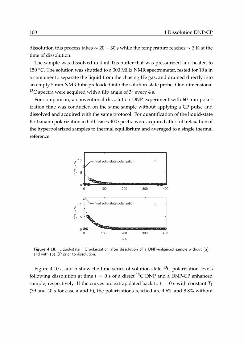
100 4 Dissolution DNP-CP
dissolution this process takes ⇠ 20 � 30 s while the temperature reaches ⇠ 3 K at thetime of dissolution.
The sample was dissolved in 4 ml Tris buffer that was pressurized and heated to150 �C. The solution was shuttled to a 300 MHz NMR spectrometer, rested for 10 s ina container to separate the liquid from the chasing He gas, and drained directly intoan empty 5 mm NMR tube preloaded into the solution-state probe. One-dimensional13C spectra were acquired with a flip angle of 3� every 4 s.
For comparison, a conventional dissolution DNP experiment with 60 min polar-ization time was conducted on the same sample without applying a CP pulse anddissolved and acquired with the same protocol. For quantification of the liquid-stateBoltzmann polarization in both cases 400 spectra were acquired after full relaxation ofthe hyperpolarized samples to thermal equilibrium and averaged to a single thermalreference.
0 100 200 300 4000
5
10
0 100 200 300 4000
5
10
P(13
C) /
%
t / s
P(13
C) /
%
final solid-state polarization
final solid-state polarization
a)
b)
Figure 4.10. Liquid-state 13C polarization after dissolution of a DNP-enhanced sample without (a)and with (b) CP prior to dissolution.
Figure 4.10 a and b show the time series of solution-state 13C polarization levelsfollowing dissolution at time t = 0 s of a direct 13C DNP and a DNP-CP enhancedsample, respectively. If the curves are extrapolated back to t = 0 s with constant T1
(39 and 40 s for case a and b), the polarizations reached are 4.6% and 8.8% without

4.4 Results 101
and with CP, respectively. Both dissolution efficiencies (63% and 72%) are similarto previously observed values [22, 24, 73] and their difference is assumed to be anexperimental variation independent of the solid-state pulse scheme. The additionalpolarization enhancement gained by the CP pulse in the solid state was thus shownto be transferable to the solution state.
4.4.3. Multiple-contact time DNP-CP
As mentioned in section 4.1.2 in this chapter and later discussed in section 5.3 theDNP-CP enhanced 13C polarization relaxes back to the DNP steady-state level afterthe CP pulse with a time constant TTM (thermal mixing time). This effect can be seenin figure 4.1 in this chapter and in figure 5.6 in chapter 5. At the same time the 1Hpolarization builds up back to the steady-state DNP level. If the rate of 1H buildup t�1
1H is faster than T�1TM than multiple-contact time CP experiments can be utilized
to further enhance the 13C polarization (multi DNP-CP). This was implemented byrepetitive applications of the entire AHP-CP block shown in figure 4.4b.
A sample of 3.6 M [1,4-13C]fumaric acid doped with 50 mM TEMPO and 16 mMtrityl (in DMSO-d6, 2 mM Gd) was found to fulfill this condition with a ratio TTM
t1H⇡ 10
at 4.2 K. Figure 4.11 shows the comparison of the 13C polarization build up usingplain DNP, single DNP-CP, and multi DNP-CP at 4.2 K. Using multi DNP-CP anenhancement of eCP = 3.5 could be achieved over the plain DNP while acceleratingthe build up by ⇠ 5. With the single DNP-CP technique an enhancement of eCP = 2and acceleration of the build up of ⇠ 12 could be achieved.
The reduced build-up of the multi DNP-CP compared to the single DNP-CP tech-nique arises from the repetitive saturation of 1H polarization. Its effect increases withincreasing CP repetition rate. Figure 4.12 shows the dependency of the achieved CPfactor and the multi DNP-CP build-up rate as a function of the CP repetition rate forthe given sample. It shows that in this case the optimum results could be obtainedwith repetition rates between 10 � 20 s.

102 4 Dissolution DNP-CP
0 50 100 150 200 250 300 350 400 450 5000
0.02
0.04
0.06
0.08
0.1
0.12
single DNP-CP: τ = 7.1 s,
ε = 338.6
effective coupling constant: TTM
= 69.3 s
multi DNP-CP:
τ = 17.7
ε = 518.4
t / s
13C
po
lariza
tion
(single) DNP-CP using AHP
Decay after DNP-CP at t=20 s
multi DNP-CP: CP every 20 s
plain DNP build up
plain DNP: τ = 87.3 s,
Figure 4.11. Comparison of plain DNP, DNP-CP, and multi DNP-CP on a sample of 3.6 M[1,4-13C]fumaric acid doped with 50 mM TEMPO and 16 mM trityl (in DMSO-d6, 2 mM Gd) at4.2 K.
0 10 20 30 40 500
2
4
CP
fa
cto
r
single DNP−CP pulse
0 10 20 30 40 500
20
40
τ / s
Repetition time between CP pulses / s
Figure 4.12. CP factor and multi DNP-CP build-up rate as a function of the CP repetition rate at 4.2K (sample as in figure 4.11).

4.5 Discussion 103
4.5. Discussion
The discussion given in section 4.1 and in the theory (section 2.2.2) lead to the con-clusion that, for the combination of CP with DNP, the TM mechanism should be pre-ferred over the SE. Two drawbacks of this mechanism become important when usedfor DNP-CP:
i) Equation 2.76 indicates an inverse dependency of e on the electron dipolar fre-quency D. It was shown by Heckmann et al. [92] that this quantity can be in-terpreted as the EPR line width Dwe. They show that equation 2.76 can be fittedto the correlation between measured deuteron enhancements and Dwe of variousradicals. If using a radical with Dwe > w1H to allow TM on 1H this line width islarger by a factor of > 4 compared to the needed line width for direct 13C DNPvia TM and, therefore, will yield a smaller DNP enhancement. This finding is inagreement to achieved enhancements published in literature that vary from 25%to 45% 13C polarization using trityl radicals [22, 28, 69, 84] and 6% to 14% forTEMPO [24, 29, 30, 33]. Thus, optimizing DNP-CP with respect to the used radi-cal could be promising, e. g., investigating the usage of galvinoxyl as suggestedby Lumata et al. [93].
ii) The shown thermal mixing between both 1H and 13C Zeeman reservoirs (fig 4.1)makes the timing of the CP - dissolution succession critical such that the delaybetween CP and dissolution should be minimized to ⌧ TTM. At temperaturesbelow 2 K the thermal mixing rate can be reduced by avoiding mw irradiation.Therefore, for dissolution DNP-CP experiments the microwave source should beturned off at the time of CP.
The partial saturation method for B1 calibration introduced in section 4.2 has beenshown to allow fast estimation of the B1 field strength for slow relaxing spin systems.Possible artifacts due to spin echoes could be avoided with a repetition rate smallerthan the nuclear line width. As a prerequisite to this method, the order of magnitudeof the calibrated B1 field has to be known.
The optimization of the Hartmann-Hahn CP by using AHP has improved the CPefficiency. In the context of dissolution DNP-CP, the often encountered restriction inrf-field strength directs the focus to low-rf CP techniques. The data presented in fig-

104 4 Dissolution DNP-CP
ure 4.8 shows a much lower decrease in the CP factor for the AHP CP sequences com-pared to the hard-90� sequence when lowering the rf-field strength and demonstratesthe advantage of using AHP sequences compared to hard-pulse sequences especiallyat low rf-field amplitudes. Further adiabatic CP techniques should be investigatedwith the aim of maximizing the achievable transfer efficiency at rf-field strengths of< 20 kHz, which should be readily achievable in dissolution DNP probes.
The polarization enhancement gained by the CP was shown to be transferrable tothe solution state. It is noteworthy that the polarization gain by DNP-CP in the liquidmight differ from the gain detected in the solid state because the nuclei in the vicin-ity of the polarizing agent, which polarize particularly well, are not detectable in thesolid due to strong paramagnetic frequency shifts. In the solution state, however, allnuclei are detected. On the other hand, the CP efficiency will most likely be low fornuclei with strong paramagnetic frequency shifts. It is difficult to predict how thecombination of these two effects will influence the observed polarization enhance-ment in solid and solution state for different samples and further investigations onthis topic should be conducted.
The acceleration of the build up and enhancement of the final 13C polarizationachievable with the dissolution DNP-CP method strongly depends on the mutualratios of t1H, t13C, and TTM as well as on the achievable 1H steady-state DNP level.These quantities vary with sample parameters such as radical concentration and de-gree of deuteration and need to be optimized for each compound and sample condi-tion. In section 4.4.3 it is shown that for a [1,4-13C] fumaric acid sample the accelera-tion of the build up can reach ⇠ 12. Furthermore, for this sample the ratio TTM
t1H⇡ 10 is
favorable for the application of multiple-contact time CP allowing CP enhancementsof up to ⇠ 3.5. Multiple-contact time CP is also applied by the group of Bodenhausento enhance the 13C sodium acetate polarization in their DNP-CP experiments [94, 95].

5. A spin-thermodynamic model ofthermal mixing
The TM mechanism as introduced in section 2.2.3 assumes that any participatingnuclear species mixes its inverse spin temperature instantly with the electron non-Zeeman bath. However, with 1H and 13C nuclei participating simultaneously in theDNP process and furthermore applying polarization transfer from one to the other,the assumption of instant coupling between the nuclear Zeeman and electronic non-Zeeman reservoir is not correct anymore.
To get a qualitative insight into the dynamics of a spin system with multiple cou-pled spin reservoirs a thermodynamic model is applied similar to the one suggestedby Goldman [96]. It is not the intention of this model to describe the physical processof polarization transfer from electrons to nuclei but to describe the interdependenceof the spin temperatures of two different nuclear spin species experiencing TM. Thischapter was partly presented in [97].
5.1. Model description
Figure 5.1 shows the considered reservoirs: the lattice L (with inverse spin tempera-ture bL), the proton and carbon Zeeman reservoirs HZ and CZ (bH and bC, respec-tively), the electronic non-Zeeman reservoir NZ (be), and an imaginary cooling reser-voir CL (bCL). The latter is a virtual reservoir, however, the process of dynamic cool-ing via microwave irradiation is assumed to be equivalent to the coupling to such avirtual cooling reservoir and the substitution is hence considered as reasonable. Thecoupling rates shown in figure 5.1 are the thermal coupling rate constants betweenNZ and both nuclear reservoirs (kC and kH), the spin-lattice relaxation rates of HZand CZ (RH and RC) and NZ (Re), and the cooling rate (RCL). CL is assumed to be
105

106 5 A spin-thermodynamic model of thermal mixing
always cooler than L (TCL < TL) and L is assumed to have infinite heat capacity. Notethat the arrows in the chosen picture indicate the flow of the inverse spin tempera-ture b rather than the spin-temperatures TS. Finally, the ability to turn microwaveirradiation on and off is included by the possibility to decouple NZ from CL.
HZ: βH
(= > εH)CZ: β
C (= > ε
C) NZ: β
e (= > ε
e)
Lattice L: βL
(= > 1)
kC
kH
RCL
Re
RH
RC
CL: βCL
(= > εCL
)
Figure 5.1. Spin-thermodynamic model with flow of inverse spin temperatures b. The 13C Zeemanreservoir (CZ), 1H Zeeman reservoir (HZ), and the electronic non-Zeeman reservoir (NZ) relax to theLattice (L) with relaxation rates RC, RH, and Re, respectively. NZ is coupled to both CZ and HZ withthe thermal coupling rate constants kC and kH and gets cooled via the microwave-induced cooling rateRCL from the cooling reservoir (CL). All inverse spin temperatures b can be substituted by the DNPenhancements e if normalizing all by the lattice inverse spin temperature bL.
The inverse spin temperatures of CZ, HZ, and NZ in the drawn model are de-scribed by a set of three coupled differential equations
bC(t) = � kCCC
bC(t) +kCCC
be(t)� RC [bC(t)� bL] (5.1)
bH(t) = � kHCH
bH(t) +kHCH
be(t)� RH [bH(t)� bL] (5.2)
be(t) =kCCe
bC(t) +kHCe
bH(t)�kC + kH
Cebe(t)� Re [be(t)� bL] + RCL [bCL(t)� be(t)]
(5.3)
with the heat capacities as the Curie constants CI = Ni4 g2
i h (as defined in equation

5.1 Model description 107
2.100 in section 2.3.2), the number of spins Ni, and the coupling constants kC and kH
between NZ and both nuclear reservoirs defining the thermal coupling rate constantsvia:
ki =kiCC
(5.4)
by normalizing the coupling constants to the 13C heat capacity. With this and usingthe polarization enhancement factors ei = bi
bL(with bL staying constant due to its
large capacity) one can rewrite equations 5.1 - 5.3 in matrix form as:
e(t) =
0
B
B
@
bC(t)bL
bH(t)bL
be(t)bL
1
C
C
A
=
0
B
@
�kC � RC 0 kC
0 � CCCH
kH � RHCCCH
kHCCCe
kCCCCe
kH �RCL � Re � CCCe(kC + kH)
1
C
A
· e(t)
+
0
B
@
RC
RH
Re + RCLeCL
1
C
A
. (5.5)
For CZ and HZ the ratios of heat capacities simplify to the product of the ratio ofthe gyromagnetic ratios and the ratio of their molarities chosen in a given sample. Forthe capacity Ce of NZ another assumption has to be made: Since NZ represents thebroadened EPR line its heat capacity is assumed to be equal to the Curie constant ofa spin-1/2 system with a Zeeman splitting according to the electron EPR line widthof ⇡ 300 MHz. Therefore:
Ce =Ne4
g2NZh with gNZ =
30035
gC
with the 13C Larmor frequency being 35 MHz in our system.

108 5 A spin-thermodynamic model of thermal mixing
5.2. Solution of the differential equations and modelfitting
The kinetics assumed in the model lead to a set of three coupled differential equationswith seven parameters shown in equation 5.5:
RC, RH, Re, kC, kH, RCL, and eCL. (5.6)
The core of the solution and parameter optimization is the numerical solution of thedifferential equations for a chosen set of seven parameters with boundary conditionsgiven by the starting conditions of the kinetic model. All equation-solving and opti-mization steps were realized with MATLAB.
For each given sample, the numerical solution routine (function ode15s) utilizes anadditional unique set of three fixed parameters defining the relative heat capacitiesof the three spin systems, normalized to the heat capacity of the carbon spins. Forsituations in which microwave irradiation is turned off, the coupling parameter RCL
is set to zero.
For parameter optimization, numerical solutions of the model were fitted to ex-perimental data. For this purpose, the algorithm (based on the function fminsearch)fitted the model simultaneously to 12 data sets: the polarization enhancement build-up and decay curves of protons and carbons of three different samples (Sample A, C,and D in table 5.1; 2 · 2 · 3 = 12 curves) each with the appropriate starting boundaryconditions. The sample compositions are summarized in table 5.1. All time-coursedata were acquired with four-step phase-cycled averaged FIDs, each with a 1� or 3.6�
excitation pulse for 1H and 13C, respectively.
The fitting was realized by minimizing the sum of the 12 norms of the differencesbetween data points and model predictions, henceforth referred to as the goodnessof the fit. Finally, the minimization routine was run 150 times with varying randomlychosen starting sets of the seven parameters to minimize the risk of finding localminima.

5.3 Results and Discussion 109
Sample Solventdeuteration
Sampledeuteration
Solvent(1/1)vol
A 0% 0% glycerol/H2O
B 20% 42% glycerol/D2O
C 50% 58% glycerol-d3/D2O
D 100% 85% glycerol-d8/D2O
Table 5.1. Sample compositions. All samples hold 4.5 M [13C]urea and 50 mM TEMPO
5.3. Results and Discussion
With 150 randomly chosen starting values of parameters given in equation 5.6 thefitting process gives 150 similar solutions for the set of parameters. Of these, 108solutions within 4% less goodness compared to the best fit were selected for furtherprocessing. The set of parameters with the best fit is given in table 5.2 and the result-ing modeled course of enhancements for all 12 data sets used for the fitting is shownin figure 5.3.
RC RH Re kC kH RCL eCL
0.0012 s�1 0.014 s�1 0.0013 s�1 0.007 s�1 26.11 s�1 5.1 s�1 198.49
±0.0001 s�1 ±0.0002 s�1 ±0.03 s�1 ±0.0002 s�1 ±9.75 s�1 ±0.14 s�1 ±4.16
(T1C = 864.7 s) (T1H = 71.3 s) (T1e = 749.9 s)
Table 5.2. Parameters of the best fit. The error given for each parameter is the standard deviation ofthe 108 solutions within 4% less goodness compared to the best fit.
The long relaxation time of the electronic non-Zeeman reservoir Re is striking in thisfit. Abragam and Goldman argue [10] that a coupled system of one nuclear Zeemanbath and an electron non-Zeeman bath relaxes with a common rate of T1,n = T1,e ·hHZihHNZi
. Herein, the ratio of the expectation values of the total nuclear Zeeman andelectronic non-Zeeman Hamiltonians should be equal to the ratio of heat capacities.From this, one would expect the relaxation rate Re to be much faster than the nuclearZeeman relaxation rates, between (0.10 s)�1 (above relation applied to n = 1H) and(600 s)�1 (n = 13C). This is not the case in the best fit shown in table 5.2, however, thevariance on this parameter is large and almost equal results are obtained for values

110 5 A spin-thermodynamic model of thermal mixing
down to Te = 10 s such that the obtained value for Re is not assumed to be unrealisticbut rather unsubstantial.
Parameter correlations were analyzed assuming linear correlations. This assump-tion was found to be a good approximation since only the small range of valuesaround the best fit was considered. The full set of Pearson’s correlation coefficientsshows mutual correlations of 2 groups of variables if the threshold for correlationis set to 75%: group I: 1,7 (positive) and 4,5 (positive) and 1,4 (negative); group II:2,3 (negative). Parameter 6 is additionally weakly correlated to the first group. Thesecorrelations are a result of the lack of data necessary to deterministically fit the model,i.e., the missing spin temperature course of the NZ reservoir.
The fitted common set of parameters solves the model simultaneously for the 3samples A, C, and D with different deuteration degree (figure 5.3) by modification ofthe heat capacity of the proton bath solely. With the fitted set of parameters further-more the behavior of the fourth sample (B) with a different deuteration degree couldbe predicted both in build-up and relaxation speed as well as in steady-state DNPenhancement on both nuclei as shown in figure 5.4. For this, only the model heatcapacity has to be modified corresponding to the actual molarity of proton nuclei inthe sample.
The model predicts for a sample with 1M 1H concentration a build up on the orderof 1 s for protons while carbons are not sped up dramatically compared to sample D.With regard to experiments utilizing cross polarization from protons to carbons sucha sample however would be unsuited since the low concentration ratio of protons tocarbons of 1/4 would lead to low CP efficiency. The measured build-up rates t of1H and 13C and their common steady-state DNP enhancement values of samples A- D are plotted in figure 5.5. In the context of the combination of DNP with CP, thisplot shows that not only the achieved common DNP value increases with increasingdeuteration but furthermore the 1H build-up time decreases, essentially acceleratingDNP-CP experiments.
The model correctly predicts the behavior of both 1H and 13C polarization after ar-bitrary experimental preparation of both nuclear spin temperatures, with and with-out microwave irradiation (figure 5.6). Specifically, it predicts that after a CP pulse the13C enhancement tends to re-equalize with the 1H enhancement within the thermalmixing time TTM (figure 5.6 a). This time constant depends on the coupling strengthof NZ to both nuclear Zeeman baths and is in general faster than the nuclear T1 (also

5.3 Results and Discussion 111
11
.5
x 1
0
0.0
12
0.0
14
0.0
16
r(1
,2)=
−0
.03
7
11
.5
x 1
0
0
0.1
0.2
r(1
,3)=
0.0
60
11
.5
7
7.5
r(1
,4)=
−0
.96
1
11
.5
x 1
0
30
40
50
60
r(1
,5)=
−0
.89
5
11
.5
x 1
0
4.55
5.56
r(1
,6)=
−0
.46
7
11
.5
x 1
0
18
0
20
0
22
0 r
(1,7
)=0
.92
8
0.0
13
0.0
14
0
0.1
0.2
r(2
,3)=
−0
.86
1
0.0
13
0.0
14
678
x 1
0-3
r(2
,4)=
−0
.04
7
0.0
13
0.0
14
20
40
60
r(2
,5)=
−0
.07
3
0.0
13
0.0
14
456 r
(2,6
)=0
.50
4
0.0
13
0.0
14
16
0
20
0
24
0 r
(2,7
)=−
0.2
82
00
.05
0.1
678 r
(3,4
)=−
0.0
34
00
.10
.20
50
10
0 r
(3,5
)=0
.01
0
00
.10
.2456
r(3
,6)=
−0
.51
7
00
.10
.21
80
20
0
22
0 r
(3,7
)=0
.36
2
6.5
77
.5
x 1
0
20
40
60
r(4
,5)=
0.9
36
6.5
77
.5456
r(4
,6)=
0.3
77
6.5
77
.51
80
20
0
22
0 r
(4,7
)=−
0.8
80
20
40
60
456 r
(5,6
)=0
.28
3
20
40
60
18
0
20
0
22
0 r
(5,7
)=−
0.7
84
45
61
80
20
0
22
0 r
(6,7
)=−
0.7
27
3.8
23
.84
3.8
63
.88
3.9
03
.92
x 1
0-3
x 1
0-3
x 1
0-3
x 1
0-3
x 1
0-3
x 1
0-3
x 1
0-3
x 1
0-3
x 1
0-3
x 1
0-3
x 1
0-3
x 1
0-3
x 1
0
Figu
re5.
2.Co
rrel
atio
npl
ots
ofth
e10
8be
stfit
s.Pl
otte
dar
epa
irwise
the
para
met
ers:
1=
RC
,2=
RH
,3=
Re,
4=
k C,
5=
k H,
6=
RC
L,an
d7=
e CL
asin
dica
ted
inth
eco
rrel
atio
nco
effici
ents
(r(x
-coo
rdin
ate,
y-co
ordi
nate
)).
Inte
nsiti
esin
the
give
nco
lorco
deco
rres
pond
toth
ein
vers
eof
the
good
ness
ofth
efit
s.A
xis
units
are
s�1 ,
unitl
ess
for
para
met
er7=
e CL.

112 5 A spin-thermodynamic model of thermal mixing
0
50
100
150
0
50
100
150
0 200 400 6000
50
100
150
t / s
0 200 400 600
t / s
1H measured
13C measured
model fits
DNP build up T1 decaysamples
(deuteration)
A
(0%)
C
(58%)
D
(85%)
Figure 5.3. Experimentally obtained 1H and 13C enhancement courses for samples A, C, and D usedto fit the model parameters. The simulated enhancement courses by the model using the best-fitparameters (table 5.2) are plotted as solid lines.

5.3 Results and Discussion 113
0 200 400 6000
50
100
150
t / s
0 200 400 600
t / s
DNP build up T1 decay
1H measured
13C measured
model predictions
Figure 5.4. Model predictions using the best-fit parameters (table 5.2) and experimentally obtainedvalues of the DNP enhancement and decay of sample B. The model used a value for the 1H heatcapacity that was adjusted corresponding to the actual molarity of 1H nuclei in the sample.
0 0.2 0.4 0.6 0.8 10
20
40
60
80
100
120
140
160
180
200
Sample protonation degree
τ / s
, ε
τ (1H)
τ (13
C)
common ε
SASBSCSD
Figure 5.5. Measured build-up rates t of 1H and 13C and the common steady-state DNP enhancementvalues of Samples A - D at 4.2 K.

114 5 A spin-thermodynamic model of thermal mixing
clearly apparent in figure 5.6 b and d). Figure 5.6 b shows that at 4.2 K the thermalmixing process is active even without ongoing microwave irradiation. In agreementto the findings by Cox et al. in 1973 [66] it shows that the 13C polarization rises after asaturation train. This behavior is well predicted by the introduced model and clearlysuggests that the samples are undergoing thermal mixing.
t / s t / s
0 200 400 600
0
20
40
60
80
ε
0 200 400 600
0
50
100
150
ε
0
20
40
60
80
100
ε
20
40
60
80
100
ε
0
1H measured
13C measured
model predictions
(a)
(b)
(c)(d)
Figure 5.6. Model predictions using the best-fit parameters and experimental values of the 1H and13C enhancement courses of sample A after different preparations. For a guide to the eye the DNPbuild-up data (a,c,d) and decay data (b) are underlayed in light grey. The model predicts well (solidlines) the enhancement course of 13C after a CP pulse at t = 90 s (a), the 13C enhancement courseafter steady-state DNP followed by a single saturation on 13C and microwaves turned off (b), bothenhancement courses after a CP pulse at t = 20 s (c), and both enhancement courses during DNPbuild up after a single saturation at t = 120 s on 1H (d).
In figure 5.6 c the CP pulse is applied at a time point such that the resulting 13Cpolarization equals the steady-state DNP enhancement. Here, the model correctlypredicts the following decrease of polarization to re-equalize both carbon and pro-ton enhancements. This shows that it is neither straightforward nor enduring to lift

5.3 Results and Discussion 115
the carbon polarization to its steady-state DNP enhancement with a single DNP-CPpulse. Finally, figure 5.6 d illustrates how the 13C polarization is effected by (par-tial) saturation of the 1H polarization as will occur during the CP step. The 13C spintemperature clearly depletes until it re-equalizes with the recovering 1H spin temper-ature.
It is worth mentioning that the model also correctly predicts the initial DNP build-up behavior of both spin baths. While the 1H polarization builds up in a mono-exponential manner, the 13C polarization was found to have an initial damped build-up rate (figures 5.3, 5.4). In the terminology of the spin-thermodynamic model thereason for this is the much weaker coupling between CZ and NZ compared to thecoupling between HZ and NZ.


6. The influence of sampleparameters on dissolution DNP
The large majority of dissolution DNP experiments nowadays is done using the tritylradical OX063 to polarize pyruvic acid. Furthermore, for methodological develop-ments and research, often derivatives of the TEMPO radical are used to polarize smallorganic molecules (for example glycine [24, 29], acetate [33], urea [22, 73]) or the sol-vents [98]. For this reason, the influence of the radical concentration and pH as wellas sample temperature of similar systems on dissolution DNP experiments will bediscussed in this chapter.
6.1. Pyruvate/trityl-based samples
6.1.1. Solid-state DNP and T1
During the process of dissolution, the sample unavoidably is being heated imme-diately before being dissolved. This is due to the necessity of coupling and sealingwarmer dissolution hardware components (in our case the grabber and the dissolu-tion stick) to the sample container.
To be able to estimate the extent of polarization losses during this period, a series of13C T1 data was acquired on samples of [1-13C]pyruvic acid doped with 0, 5, 10, and15 mM trityl. The experiments were conducted using the probe 2 in combination withthe NMR stick (see section 3.5.2). The system temperature was stabilized at varioustemperatures between 1.4 K and 70 K while at each temperature T1 experiments wereconducted successively on the samples using the revolver rotation mechanism. Thepulse scheme used was a saturation recovery sequence using aperiodic saturationas described in [99, 100]. Signal intensities (peak integrals) were fitted with mono-exponentials.
117

118 6 The influence of sample parameters on dissolution DNP
6.1.2. Liquid-state T1 dependence on pH
The applicability of the dissolution DNP method in combination with solution-stateNMR or MRI techniques is essentially determined by the solution-state T1 relaxationrate of the polarized nuclei. It has been shown that for polarized amino acids thepolarization loss during shuttling in low field is strongly dependent on pH and in-creases considerably for basic solutions [32].
Over a period of 2 years the solution-state T1 values of polarized and dissolved[1-13C]pyruvic acid samples were observed in numerous referencing phantom ex-periments in our lab. In each experiment the samples were shuttled to a 9.4 T MRIafter dissolution and the decaying polarization was monitored with low-flip anglemeasurements (4�). The experiments were conducted by varying teams mainly com-posed by Marcin Krajewski, Kilian Weiss, Giorgos Batsios, Lukas Wissmann, JuliaBusch, and me. The polarized samples were neat pyruvic acid doped with 13.5 to15 mM trityl and 1.5 mM Gd with a dissolution ratio of ⇠ 1/160 (only 5 sampleswere dissolved with ⇠ 1/320, mainly having neutral pH). They were dissolved in abuffered solution (tris + NaCl + EDTA) and mixed with neutralizing NaOH imme-diately after dissolution next to the DNP magnet before carrying them manually tothe MRI. Figure 6.3a shows the correlation of T1 values and the pH values that weremeasured after the solution-state acquisition had finished.
Furthermore pH-dependent relaxometry was carried out in a 200 MHz solution-state NMR probe. Samples of 83 mM [1-13C]pyruvic acid in the tris-buffer solutionwere prepared to mimic the dissolved pyruvic acid solution (no trityl radicals, 5%D2O added). Samples of different pH were prepared from the same stock by addingcertain amounts of NaOH to achieve pH values of: 1.7 (no NaOH), 2.1, 3.9, 6.8, 7.7,9.4, and 12.3. Saturation recovery measurements were conducted while retaining thesample temperature at constant 310 K (to mimic body temperature).
6.1.3. Results and discussion
Solid-state DNP and T1
Figure 6.1 shows the measured T1 relaxation rates as function of the temperature.Due to excessive relaxation times of the 0 mM and 5 mM samples no data has beenacquired at 1.4 K for these samples. Figure 6.1 reveals a strong temperature depen-

6.1 Pyruvate/trityl-based samples 119
dence of all samples, including the one without trityl. This points to the fact that, forthe investigated samples, there is a relaxation pathway alongside the relaxation viathe paramagnetic radicals that contributes strongly to the T1 relaxation. The sourceof this is assumed to be the methyl rotations of the pyruvic acid methyls. Further-more, at temperatures around 4 � 8 K there appears a range of fast relaxation for allsamples, again pointing to another source of relaxation alongside the paramagneticrelaxation.
101 102
101
102
103
104
Temperature / K
13C
T1 / s
0 mM trityl
5 mM trityl
10 mM trityl
15 mM trityl
Figure 6.1. Longitudinal relaxation times of [1-13C]pyruvic acid doped with 0, 5, 10, and 15 mM tritylas a function of temperature. The error on all data points is ⇠ 10% arising from the fitting error.However, the reproducibility of the measurements upon repeated sample freezing has been shown to beless accurate than these 10%.
The fast relaxation both at 4 � 8 K and at higher temperatures shows the impor-tance of a fast dissolution protocol. For this reason, the dissolution protocol had to beoptimized by i) reducing the time of thermal contact between the dissolution hard-ware and the sample container to below 5 s (of which only < 1 s is the contact be-tween dissolution stick and sample container) and ii) by precooling of the dissolutioncomponents (as is achieved by introduction of the cold grabber described in section3.5.7).

120 6 The influence of sample parameters on dissolution DNP
4 5 6 7 8 9 10 11 12 13 14 15 16 17 18 19 20 21 22 23 24 25 260
200
400
600
800
DN
P b
uild
up
tim
e / s
4 5 6 7 8 9 10 11 12 13 14 15 16 17 18 19 20 21 22 23 24 25 260
200
400
600
800
T1 r
ela
xatio
n tim
e / s
4 5 6 7 8 9 10 11 12 13 14 15 16 17 18 19 20 21 22 23 24 25 260
50
100
150
200
250
DN
P e
nh
an
cem
en
t
Trityl concentration / mM
a)
b)
c)
Figure 6.2. DNP build-up times, T1 relaxation times, and steady-state DNP enhancements at 3.47 Kon samples of [1-13C]pyruvic acid with trityl concentrations ranging from 5 mM to 25 mM. The differentsymbols and colors group the data points into groups acquired during the same experimental sessionand prepared from the same stock solutions.

6.1 Pyruvate/trityl-based samples 121
Further samples of [1-13C]pyruvic acid with trityl concentrations ranging from 5 mMto 25 mM were measured at 3.47 K. In these experiments T1 values were extractedfrom mono-exponential fits to the decay curves after DNP enhancement (figure 6.2b).From the same DNP build-up and decay experiments build-up rates and steady-stateDNP enhancement values were measured on those samples (figure 6.2a and c). Thelarge error bars on figure 6.2c arise from the low reproducibility of DNP enhance-ments upon reloading the system with the same samples. This is mainly due to thefact that in these experiments the samples were scanned in the dissolution port posi-tion using the NMR stick. The bump of DNP enhancements around 16 mM thus hasto be taken with care and understood as tendency.
Liquid-state T1 dependence on pH
The correlation of the solution state T1 with the sample pH both measured in 9.4and 4.7 T are shown in figure 6.3. Both figures 6.3b) and a) show a similar depen-dence. The data sets indicate the importance of neutral pH during acquisition in theMRI/NMR after dissolution and hence care has to be taken to adjust the pH of thedissolved sample by adding the correct amount of base immediately after dissolution.
0 2 4 6 8 10 12 140
5
10
15
20
25
30
35
40
45
50
pH
Liq
uid
T1 (
in 9
.4 T
) / s
0 2 4 6 8 10 12 140
10
20
30
40
50
60
Liq
uid
T1 (
in 4
.7 T
) / s
pH
a) b)
Figure 6.3. Correlation of solution-state T1 and sample pH (T1 values are given with 10% error esti-mated from the monoexponential fitting variance). a) T1 after dissolution DNP experiments measuredin a 9.4 T MRI. All samples contain dissolved [1-13C]pyruvic acid (final concentration of ⇠ 90mM)and traces of trityl radical (< 100 µM) in a tris buffer. b) T1 measured in a 4.7 T at 310 K of samplescontaining 83 mM [1-13C]pyruvic acid in tris-buffer solution (without trityl radicals, 5% D2O added).
For in-vivo MRI experiments the pH has to be adjusted roughly to physiological pH7.3� 7.4 [101],[102, p. 146]. The presented data shows that this is the optimum region

122 6 The influence of sample parameters on dissolution DNP
concerning T1 as well.
Low-field pH-dependent relaxometry on pyruvic acid samples would help under-standing the relaxation dependence during the shuttling processes. Similar low-fieldrelaxometric data has been published on [1-13C]acetate doped with up to 2.5 mMof the TEMPOL radical by Mieville et al. [103]. The relaxation pathways and theirstrength however strongly depend on the molecule of interest, the paramagneticdopand, and the solvent. Therefore, care has to be taken when attempting to applythe findings of Mieville to pyruvic acid samples.
6.2. TEMPO-based samples
Samples doped with the TEMPO radical were chosen in this work for the combi-nation of dissolution DNP with CP. For this reason, samples of 4.2 M [13C]urea in(1/1)vol glycerol-d3/D2O with radical concentrations between 20 � 70 mM were an-alyzed regarding their solid-state DNP values, CP efficiency, dissolution efficiency,and solution state T1.
6.2.1. Solid-state DNP enhancement
Samples containing 30, 45, and 70 mM were polarized in the probe 1 at single shottemperatures. Note that in this probe the temperature sensor mounted on the probereads 1.5� 1.7 K during microwave irradiation whereas the temperature sensor moun-ted on the cryostat remains at its low temperature reading (1.2 � 1.3 K). Thus, theexact temperature during these experiments cannot be determined more accuratelythan giving the range 1.3� 1.7 K or stating < 1.7 K. The 13C NMR signal intensity wasfollowed with low-flip angle measurements (< 4�) every 30 s without microwaveirradiation. After having acquired a large enough amount of thermal equilibrium ref-erence spectra the microwaves were turned on to the optimum frequency (⇠ 93.900GHz, depending on the sample) and field strength (120 mW) previously determined.After reaching the DNP steady state, the microwaves were switched off to determinethe T1 relaxation rate.

6.2 TEMPO-based samples 123
6.2.2. CP efficiency
For samples containing 30 and 70 mM TEMPO the CP transfer was optimized andcompared at single-shot temperatures (1.3 � 1.7 K) and 4.2 K in probe 1. The CPtransfer was done using the AHP pulses with a maximum rf-field amplitude and CPmixing field strength of 100 kHz.
6.2.3. Dissolution efficiency
On the probe 2 the dissolution efficiency was compared for the urea samples contain-ing 20, 30, 40, 60, and 70 mM TEMPO with and without CP following the DNP at 1.35K. The experiments were conducted following the procedure described in section 4in combination with automatic shuttling to a 7 T NMR spectrometer. Microwavefrequency and irradiation times were set to the optimum for each sample and theCP sequence was used with AHP pulses with a maximum field strength and mixingfield of 30 kHz. The dissolution efficiency was calculated as the ratio between the 13Cpolarization in the liquid state (back extrapolated to time point t = 0 after dissolu-tion, see section 4) and the 13C polarization measured immediately before dissolution(for the DNP-CP experiments after the CP pulse). Thereby, the polarization in theliquid state can be determined accurately since the thermal equilibrium data has ahigh enough SNR. The solid-state polarization values without CP were assumed tocorrespond to the ones quantified in the probe 1 at single shot temperature, i.e. withe ⇠ 80. The solid-state polarization after the CP pulse was calculated by multiplyingthe corresponding observed CP factor with the plain DNP polarization value.
6.2.4. Results and discussion
Solid-state DNP enhancement
The solid-state DNP enhancements of the samples containing 30, 45, and 70 mMTEMPO as well as the time constants of the mono-exponential fits to the DNP build-up and decay curves are shown in figure 6.4. For the given range of radical concen-trations the enhancement does not change considerably. The time constants howeverincrease by 500% (t) and 1200% (T1) when reducing the TEMPO concentration from70 to 30 mM.

124 6 The influence of sample parameters on dissolution DNP
Comparable experiments were published by Kurdzesau et al. on sodium acetatedoped with 17, 33, and 50 mM TEMPO [29]. While for the build-up time similarvalues were found, the DNP enhancement at 33 mM in their publication is twice ashigh as at 17 and 50 mM, both comparable to the results shown here.
20 30 40 50 60 70 800
20
40
60
80
100
TEMPO concentration / mM
0
1000
2000
3000
t / s
DNP enhancement εT
1
τDNP
13 C
en
ha
nce
me
nt
ε
Figure 6.4. Solid-state 13C DNP build-up rate, steady-state enhancement, and T1 relaxation rate at1.3� 1.7 K of samples containing 4.2 M [13C]urea in (1/1)vol glycerol-d3/D2O doped with 20, 45, and70 mM TEMPO.
CP efficiency
For CP the most important parameter to be optimized when changing the radical con-centration was found to be the CP mixing time. Figure 6.5a shows for both samplesthe CP transfer as a function of the mixing time at single-shot temperature. It showsthat the optimum mixing time shifts strongly from ⇠ 2000 µs to ⇠ 750 µs when goingfrom 30 to 70 mM TEMPO concentration. Furthermore the achievable CP factor isreduced as shown in figure 6.5b for both temperatures.
To investigate the source of the reduced CP efficiency at large radical concentrationsT1,r measurements were conducted on both samples at both temperatures with thesame protocol as described in section 4.3.2. The T1,r data were fitted with exponentialdecay curves and the corresponding time constants are plotted in figure 6.6. The

6.2 TEMPO-based samples 125
T1,r values decrease strongly for increasing TEMPO concentration. This enhancedrelaxation rate in the rotating frame explains the efficiency loss of the CP transfer forhigher radical concentrations seen in figure 6.5b. Additionally plotted in figure 6.6are the optimum mixing times for the AHP CP sequence, decreasing with increasingTEMPO concentration in the same manner and once more emphasizing the need tooptimize this parameters upon changes of the radical concentration.

126 6 The influence of sample parameters on dissolution DNP
20 30 40 50 60 70 800
0.5
1
1.5
2
2.5
3
TEMPO concentration / mM
CP
fa
cto
r
CP factor 4.2 K
CP factor < 1.7 K
b)
0 1000 2000 3000 40000
0.5
1
1.5
2
2.5
3
t / µs
CP
fa
cto
r
30 mM TEMPO
70 mM TEMPO
a)
( < 1.7 K)
Figure 6.5. a) The CP transfer as function of the mixing time at < 1.7 K for the samples containing30 and 70 mM TEMPO. b) The optimized CP factors for both samples at < 1.7 K and 4.2 K using theAHP pulses CP with 100 kHz mixing field strength.
20 40 60 800
500
1000
1500
2000
2500
t / m
s
20 40 60 80
T1ρ
opt. mixing time * 1000
TEMPO concentration / mM
< 1.7 K 4.2 K
Figure 6.6. 13C T1,r relaxation times (⇤) and optimum CP mixing times (⇤) for the samples containing30 and 70 mM TEMPO at < 1.7 K and 4.2 K.
6.2 TEMPO-based samples 127
Dissolution efficiency
Figure 6.7a shows the calculated dissolution efficiencies for all samples (other than the20 mM sample on which no DNP-CP experiment was conducted). The data shows aclear tendency on all samples of decreasing dissolution efficiency with increasing rad-ical concentration. The drop in efficiency from the 30 to 70 mM sample is as large as1/3.2. In figure 6.7c the solution-state 13C T1 relaxation times are plotted as acquiredby following the decaying hyperpolarized NMR signals after the dissolutions.
10 20 30 40 50 60 70 800
0.05
0.1
So
lutio
n p
ola
riza
tion
(t=
0 a
fte
r D
iss.
) / %
10 20 30 40 50 60 70 800
0.5
1
Dis
solu
tion
effic
ien
cy
TEMPO concentration / mM
10 20 30 40 50 60 70 8020
30
40
50
So
lutio
n s
tate
T1
/ s With CP
Without CP
a)
b)
c)
Figure 6.7. The dissolution efficiency (a) and final reached 13C polarization levels (b) upon dissolutionDNP-CP experiments conducted on samples containing 4.2 M [13C] urea in (1/1)vol glycerol-d3/D2Owith radical concentrations between 20 � 70 mM. Additionally the solution-state T1 values are plottedin c) as acquired during the relaxation of the hyperpolarized samples in the 7 T spectrometer.

128 6 The influence of sample parameters on dissolution DNP
Together with the loss in CP transfer efficiency with larger radical concentrationsseen in figure 6.5 the final solution state DNP-CP 13C polarization shown in figure6.7b reveals a strong inverse dependency on the radical concentration.
The dependence of the dissolution efficiency on the radical concentration mightbe a unique feature of the experimental setup chosen in these experiments, i.e. theexact pathway of the dissolved sample through the low-field area between the DNPmagnet and the NMR magnet. Furthermore, the speed of the shuttling might be acrucial parameter in these experiments in the sense that it might influence the relativedifferences in dissolution efficiencies observed at different radical concentrations.

Conclusion
In this thesis a cryogenic multi-sample DNP system was realized with heteronuclearNMR, EPR, and dissolution capabilities. Dissolution DNP was combined with a mod-ification of the Hartmann-Hahn cross polarization technique using adiabatic half-passage pulses. Finally, a spin-thermodynamic model was applied and the impactof sample parameters on the dissolution DNP-CP method was measured to improvethe overall efficiency of dissolution DNP-CP experiments.
Instrumentation
In chapter 3, the realization of the DNP setup is described. The cryogenic systemwas designed to fit wide-bore NMR magnets and is therefore transferrable betweencompatible magnets.
Two DNP probes have been realized: a single-sample probe allowing static het-eronuclear solid-state NMR experiments with high sensitivity and rf-field strengthsup to 100 kHz and a multi-sample DNP probe with low-sensitivity NMR, EPR anddissolution capabilities.
The revolver-style sample changer of the multi-sample probe has been shown toreliably allow exchange of samples between the DNP, CP, and dissolution sites atthe operating temperature and pressure ranges of the system. The multi-sampleprobe has been found to be highly convenient to conduct series of solid-state DNPexperiments with varying sample compositions, since the time-consuming changingof samples can be avoided. Furthermore, conducting multiple dissolution DNP ex-periments during one working day is eased by the possibility of a single loadingprocedure of all samples at the beginning of the working day.
The incorporation of an oversized microwave cavity allows efficient microwaveirradiation with minimized heating of the sample space. An EPR coil allows longitu-dinal detected EPR experiments down to 4-10 K which is important for testing DNP
129

130 Conclusion
in combination with new radicals or mixtures of radicals. The presented dissolutionDNP system has proven to reach 13C polarization levels of up to 45% in the solid stateand 33% in the solution state.
For the purpose of increasing the repetition rate of subsequent dissolutions, themulti-sample probe has shown the need for improvements. Although simultaneouspolarization of all 6 samples was shown to be possible, the dissolution of one samplemeans losses in polarization of the remaining samples and makes dissolutions DNPexperiments with a high repetition rate unfeasible. This problem could be addressedby making the dissolution conductible under vacuum conditions.
Dissolution DNP-CP
In chapter 4, aspects of the combination of CP with dissolution DNP are discussed.It is concluded that thermal mixing is the most favorable mechanism for DNP-CPexperiments while emphasizing two drawbacks of this mechanism: i) the necessityof large-line width radicals reduces the achievable direct DNP enhancements and ii)the thermal mixing between the 1H and 13C Zeeman reservoirs leads to the demandof minimizing the delay between CP and dissolution to ⌧ TTM.
A partial saturation method for calibration of rf-flip angles is introduced and shownto allow time-efficient estimation of the B1-field strength when using slow-relaxingsamples. It is, therefore, a convenient method for rf-field strength estimation in low-temperature DNP or NMR experiments.
To allow efficient application of the CP method under the limited rf-field strengthsavailable in the dissolution DNP probe, it is shown that adiabatic half-passage pulsesare able to enhance the Hartmann-Hahn CP transfer efficiency, especially at low rf-field strengths. The DNP-CP technique using adiabatic half-passage pulses is shownto allow acceleration of the polarization build up while reaching higher final 13C po-larization levels. It is shown that the solid-state CP enhancement can be transferredto the solution state via dissolution.
A spin-thermodynamic model of thermal mixing
In chapter 5, a spin-thermodynamic model based on the thermal mixing mechanismis applied to TEMPO-based samples. By varying the thermal capacity of the proton

Conclusion 131
Zeeman bath, the model correctly predicts the effect of solvent deuteration and pro-vides an intuitive understanding of the reason for the enhanced DNP efficiency uponsample deuteration. The presented model, furthermore, correctly predicts the courseof spin temperatures after various preparations of the nuclear polarizations.
The successful prediction of the dynamics of the spin system during DNP experi-ments is understood as an indication for thermal mixing to be the dominant mecha-nism on both 1H and 13C in TEMPO-based samples.
The influence of sample parameters on dissolution DNP
In chapter 6, solid-state T1 and DNP performance values are presented for trityl-doped pyruvic acid samples. The shown data emphasizes the importance to mini-mize the time of sample exposure to hot dissolution components during the dissolu-tion procedure.
Solution state T1 values as a function of the sample pH are shown for the commonlyused trityl-doped pyruvic acid sample at 9.4 and 4.7 T. The data indicates that longestT1 values are reached at neutral pH.
The DNP, CP, and dissolution efficiencies of TEMPO-doped samples are presentedas a function of radical concentration. A significant decrease of the overall efficiencyof the dissolution DNP-CP experiment towards larger radical concentrations is ob-served for the given sample compositions and experimental protocol.
The discussions throughout this thesis additionally lead to the conclusion that forTEMPO-based samples the dominant DNP mechanism is thermal mixing, both on1H and 13C. This conclusion arises once from the theoretical discussion given in sec-tion 2.2 concluding that the DNP enhancement is independent of the nuclear g forthermal mixing while being inverse dependent for the solid effect, while the datapresented in section 4.4 shows that the experimental enhancement reached is equalon both 1H and 13C . The same argument holds for the cross effect, whose contribu-tion has been shown to drop even bellow the solid effect bellow 20 K for a similarsystem [53]. Additionally, equal polarization levels of both nuclei in similar systemsusing TEMPO have been reported [29], whereas for the trityl radical the enhancementon 13C has been reported to be >10 fold compared to the 1H enhancement [27]. Sec-ond, the possibility of fitting and predicting experimental DNP data with the spin-

132 Conclusion
thermodynamic model presented in chapter 5 indicates that thermal mixing is thedominant mechanism.

Outlook
To push the dissolution DNP method towards the overall aim to which this work wasdirected, i.e., the achievement of large solution-state polarization values at a high rep-etition rate, further work has to be done on the hardware as well as on the method-ological side.
The dissolution DNP system presented in chapter 3 has shown to allow operat-ing temperatures of down to ⇠ 1.3 K. This is a value similar to what is reached byother published dissolution DNP systems [22, 24, 25, 104] and possible to be loweredconsiderably only with much more dedicated cryostat designs [28, 84]. A problemarising from the actual design of the presented multi-sample probe is the depletion ofpolarization of the remaining samples upon dissolution of one sample. To tackle thisproblem, the design presented by Marcin Krajewski [85] should be supported andadvanced. It is based on multiple independent dissolution paths that couple and sealeach to one of the simultaneously polarized samples similar as in [84].
To enhance the repetition rate of dissolution DNP experiments, it is shown in chap-ter 4 that DNP-CP is a possible complementing approach to the multi-sample de-sign. The lack in achieved 13C polarization values, however, makes further devel-opments on this technique necessary. On the hardware site, the group of GeoffreyBodenhausen (EPFL, Lausanne) recently showed [95, 105], that applying the DNP-CP technique in a magnetic field close to 7 T can lift the final reached polarizationto similar values as achieved for trtityl-based samples in common 3.4 T dissolutionDNP systems but with higher build-up rates. Therefore, the development of a high-field dissolution DNP system allowing heteronuclear NMR experiments would bepromising.
On the methodological site, further investigations should be conducted to enhancethe efficiency of the DNP-CP technique. As emphasized in section 3.5.5 and 4.5, rf-limitations are often encountered in dissolution DNP probes. CP techniques shouldthus be investigated allowing efficient polarization transfer at lower rf-field strengths.
133

134 Outlook
A method recently suggested by Lee and Khitrin [106, 107] applies adiabatic demag-netization and remagnetization in the laboratory frame (ADLF/ARLF), a techniquebased on adiabatic demagnetization in the rotating frame [108] similar to the "totalCP" experiment [109]. The advantage of full adiabatic CP techniques is the theoreti-cal increase of the CP transfer factor by
q
NINQ
over the Hartmann-Hahn CP such that1H to 13C enhancements of up to 15-fold have been reported in static powder adaman-tane [110]. Using the approach chosen by Lee and Khitrin, furthermore, allows theexperiment to be conducted at much lower rf-field strengths, e.g., below 10 kHz intheir case. Further research along this line could both, improve the final polarizationvalues as well as reduce the demands on rf-field strengths.
It is discussed in section 4.5 that large EPR line widths allow the polarization of 1Hvia thermal mixing but reduce the DNP enhancements reached for all participatingnuclei. In DNP-CP experiments it is, therefore, beneficial to use radicals with linewidths larger but similar to the 1H Larmor frequency. Lumata et al. investigated theusage of galvinoxyl for the use of DNP and showed that its line width is intermediateto the one of trityl and TEMPO [93]. Investigations on the usage of galvinoxyl orradicals with similar line widths for DNP-CP experiments could further increase theDNP-CP efficiency.
The spin-thermodynamic model presented in chapter 5 could be extended by in-cluding predictions for the rate constants. Alternatively, it could be used to gaininformation about the correlation between sample parameters and the rate constants.Further improvements in this direction could be achieved if the inverse spin temper-ature of the electron non-Zeeman reservoir could be accessed experimentally, e.g., byline shape analysis. These investigations should be directed to solving the questionif it is possible to enlarge the thermal coupling between the electron non-Zeemanand the 1H Zeeman reservoir while reducing the corresponding coupling to the 13Creservoir. This way, faster 1H DNP and thus DNP-CP to 13C could be achieved andmultiple-contact time CP could be applied more efficiently.
The standard sample used in dissolution DNP today is [1-13C] pyruvic acid. There-fore, all further developments of the DNP-CP technique should be focused on opti-mizing the efficiency on this sample. The results shown in section 6.2.4 on the disso-lution efficiency of TEMPO-based samples are alerting concerning the usage of largerradical concentrations. Compared to the results published by the Bodenhausen group

Outlook 135
[95], the efficiency achieved in the experiments presented here are low. The reasonfor this should be investigated to avoid similar losses on pyruvic acid based sam-ples. Measurements of the T1 values of a suited sample as a function of low magneticfields would provide valuable information in the context of such investigations. Apromising approach should be the scavenging of the TEMPO radicals upon dissolu-tion as suggested by Mieville et al. [103, 111]. With their approach, they are able toextend, both, the T1 and T2 relaxation times in the solution state at high and low (2mT) magnetic fields.
The placement of the DNP project within the group of solid-state NMR at the ETHfinally stimulates the application of solid-state DNP as a complementing techniqueto MAS NMR. A current open problem of the research group is the determinationof the torsion angle between the two phenyl rings of congo red when bound to anamyloid fibril. Similar to the work presented by Potapov et al. [112], one can usestatic DNP-enhanced double-quantum and single-quantum spectra (DOQSY) [113]to measure CSA tensor correlations. For this method to work, however, the spectralresolution should be large enough to resolve the CSA tensors. The development ofthe high-field DNP system suggested previously could support such a project.


Appendices
137


A. Cryogenic heat flow
The heat flow through a small temperature difference is given by the general formula:
Q = �s(T) · A(x) · dTdx
. (A.1)
The heat conducted through an object in x-direction from a plane at x1 at temperatureT1 to x2 at T2 thus can be calculated [114] as:
Q = �G [S(T2)� S(T1)] (A.2)
where G is a geometry function defined by
G =
Z x2
x1
1A(x)
dx��1
(A.3)
with the variable cross section A. S is the integrated thermal conductivity
S(T) =Z T
0s(T0)dT0 (A.4)
with the temperature-dependent thermal conductivity s.For a uniform body in x-direction with cross-section A the geometry factor simpli-
fies toG =
(x2 � x1)A
(A.5)
so that the heat flow over L = x2 � x1 can be calculated with the formula
Q = �AL[S(T2)� S(T1)]. (A.6)
A further simplification could be done by the assumption of s =constant. For mostmaterials this is a bad approximation. Especially in liquid-helium applications in
139

140 A Cryogenic heat flow
general it does not hold since large temperature differences are achieved. However,for parts of the cryogenic systems discussed in this work that experience only modesttemperature differences it might be applicable and one can use:
Q = �AL
s DT. (A.7)
To calculate the heat flow through a specific material its exact s(T) has to be known.This, however, depends strongly on the fabrication process, which means that thethermal conductivity functions given in the literature should only be used for estima-tions. For the purpose of this work this is sufficient. Figure A.1 shows an overview ofsome common materials (source: Lake Shore Cryotronics, "Cryogenic Reference Ta-bles"). For the same material figure A.2 gives the integrated thermal conductivities.
To calculate the heat conducted from room temperature to < 4 K the term
[S(⇠ 300K)� S(< 4.2K)]
can be approximated by S(300K). Therefore, equation A.6 can be simplified to
Q = �AL
S(300K). (A.8)
Additionally to the values shown in figure A.2 the following values shall be given:
1. Silver: S(300K) ⇡ 100 000 (drawn) - 360 000 (annealed) Wm [115],
2. Carbon fibres - A: S(300K) ⇡ 100 - 7500 (mean: 1500 Wm (data calculated from
[116] using S(300K) = 12300 · s(300K) by linearly approximating and extrapo-
lating the time dependence given).
3. Carbon fibres - B: S(300K) ⇡ 900Wm (data calculated as above, from [117])

141
Figure A.1. Thermal conductivities of selected materials. Source: Lake Shore Cryotronics, "CryogenicReference Tables"

142 A Cryogenic heat flow
Figure A.2. Integrated thermal conductivities of selected materials. Source: Lake Shore Cryotronics,"Cryogenic Reference Tables"

A.1 Heat flow through a succession of materials 143
A.1. Heat flow through a succession of materials
For electrical cryogenic components low thermal and high electrical conductance isdesired. This demand can be addressed by using compromising materials which havemedium thermal and electrical conductivities (for example CuBe). Another approachis the succession of different materials over the entire conducting path. The estima-tion of the resulting heat flow of a succession of two materials M (warm end at T2)and N (cold end at T1) of length m and n (L = m + n) shall be given here.
The heat flow through both materials is given with equation A.6
Qm = �Amm
[Sm(T2)� Sm(Tx)] (A.9)
Qn = �Ann
[Sm(Tx)� Sn(T1)] (A.10)
with the temperature at the junction Tx. To conserve energy, both heat flows have tobe equal:
Amm
[Sm(T2)� Sm(Tx)] =Ann
[Sn(T2)� Sn(Tx)] . (A.11)
Equation A.11 can be solved numerically for the junction temperature Tx if both in-tegrated thermal conductivities Si are known. With Tx the heat flow can be calculatedusing equation A.6.


B. Cavity dimensions
The exact dimensions of the microwave cavity of probe head 2 are given in the fol-lowing. These dimensions were used for the simulations shown in figure 3.8 b.
145

146 B Cavity dimensions
A ( 5 : 1 )
11
22
33
44
55
66
AA
BB
CC
DD
NA
ME
DA
TUM
MA
TER
IAL
DA
TEI
Kavität O
berteil A21.08.2008
AN
HU
Messing
3:1
LPC-ETH
3.00
A
21,2
R9,5
R1,5
5,2
2 R1,5
8,91
R8,5
3,3
25,8(
)
25
1,55
1,5
13,5
16,25
19
16,5
18,75
13,5
9,59,5
1111
129,5 11
1,5
1,11,11H7
1,11H7
1,1
1,1
1H7
1,1
1H7
1M
2,2
1,3
1,3
2,5
45°
6,85
2,4
17,8Ø
9,5
3
12
9
20,5
24,5
45°-0,5°0,0°
+
R1
1,3
3,2( )
Bohrungen stirnseitig
siehe Zeichnung 3.03
13,312,5
Kontur senkerodieren
Innenkontur, W
ellenleiterscharfkantiggratfrei
14,07(
)
2
2
16,2
30
Rohteil 35 lang
14,2
F0,01
N6
Pos. 3.001 S
tk.FigureB
.1.Technicaldraw
ingofthe
upperpart
Aofthe
microw
avecavity
ofprobe2
(byA
ndreasH
unkeler).

1471 1
2 2
3 3
4 4
5 5
6 6
AA
BB
CC
DD
NA
ME
DA
TUM
MA
TER
IAL
DA
TEI
Kav
ität O
berte
il b
21.0
8.20
08
AN
HU
Mes
sing
3:1
LPC-ETH
3.01
47,71
1,8
1,8
R1,
5
R9,
5
R8,
5 R1,
5R
1
1,2
3
1220,5 ()
24,5
9
12,5
13,3
25,8
()
25
Boh
rung
en s
tirns
eitig
sieh
e Ze
ichn
ung
3.56
1,5
13,5
16,25
19
1,513,5
16,5
18,75
1,55
1H7
1H71H7
1H7
1 M
1 M
1 M 1 M
129,
5
11 9,5
9,5 11
11
45°
- 0,5
°0,
0°+
3,3
4
1 M
1 M
1 M
Inne
nkon
tur
scha
rfkan
tiggr
atfre
i13,8
30
Roh
teil
35 la
ng
14,0
7(
)
F0,
01N
6
Pos
. 3.0
11
Stk.
45°x
35.2
6°
1,7
Figu
reB
.2.
Tech
nica
ldra
win
gof
the
uppe
rpa
rtB
ofth
em
icro
wav
eca
vity
ofpr
obe
2(b
yA
ndre
asH
unke
ler)
.

148 B Cavity dimensions
NAME
DATUM
MATERIAL
DATEI
Kavität Unterteil21.08.2008
ANHU
Messing
4:1
LPC-ETH 3.02
A A
6
69
5
6,5
17Ø
19Ø
14Ø
45° - 0,5°0,0°+
1Ø
1,6M
60°
2Ø
2,5 3,6
0,8Ø
1,35
- 0,10,0
+
10,5
2Kugel Ø
Scharfkantiggratfrei
Pos 3.026 Stk.
R0,56,
5
1,5
18,3Ø
1,4
Øx9
0°
Figure B.3. Technical drawing of the lower part of the microwave cavity of probe 2 (by AndreasHunkeler).

Bibliography
[1] Bouchiat, M. A., T. R. Carver, and C. M. Varnum, 1960. Nuclear Polarization inHe-3 Gas Induced by Optical Pumping and Dipolar Exchange. Physical ReviewLetters 5:373–375.
[2] Bhaskar, N. D., W. Happer, and T. Mcclelland, 1982. Efficiency of Spin Exchangebetween Rubidium Spins and Xe-129 Nuclei in a Gas. Physical Review Letters49:25–28.
[3] Kauczor, H. U., R. Surkau, and T. Roberts, 1998. MRI using hyperpolarizednoble gases. European Radiology 8:820–827.
[4] Bowers, C. R., and D. P. Weitekamp, 1987. Para-Hydrogen and Synthesis AllowDramatically Enhanced Nuclear Alignment. Journal of the American ChemicalSociety 109:5541–5542.
[5] Natterer, J., and J. Bargon, 1997. Parahydrogen induced polarization. Progressin Nuclear Magnetic Resonance Spectroscopy 31:293–315.
[6] Haupt, J., 1972. New Effect of Dynamic Polarization in a Solid Obtained byRapid Change of Temperature. Physics Letters A A 38:389.
[7] Haupt, J., 1973. Experimental Results on Dynamic Polarization in a Solid byVariation of Temperature. Zeitschrift Fur Naturforschung Section a-a Journal ofPhysical Sciences A 28:98–104.
[8] Tomaselli, M., C. Degen, and B. H. Meier, 2003. Haupt magnetic double reso-nance. Journal of Chemical Physics 118:8559–8562.
[9] Lawler, R. G., 1967. Chemically Induced Dynamic Nuclear Polarization. Journalof the American Chemical Society 89:5519.
149

150 Bibliography
[10] Abragam, A., and M. Goldman, 1978. Principles of Dynamic Nuclear-Polarization. Reports on Progress in Physics 41:395–467.
[11] Overhauser, A. W., 1953. Polarization of Nuclei in Metals. Physical Review92:411–415.
[12] Carver, T. R., and C. P. Slichter, 1956. Experimental Verification of the Over-hauser Nuclear Polarization Effect. Physical Review 102:975–980.
[13] Jeffries, C. D., 1957. Polarization of Nuclei by Resonance Saturation in Param-agnetic Crystals. Physical Review 106:164–165.
[14] Abragam, A., and W. G. Proctor, 1958. Une Nouvelle Methode De PolarisationDynamique Des Noyaux Atomiques Dans Les Solides. Comptes Rendus Hebdo-madaires Des Seances De L Academie Des Sciences 246:2253–2256.
[15] Provotorov, B. N., 1961. Nuclear Magnetic Resonance in Solids. Optika I Spek-troskopiya 11:123–125.
[16] Borghini, M., 1968. Spin-Temperature Model of Nuclear Dynamic PolarizationUsing Free Radicals. Phys. Rev. Lett. 20:419 – 421.
[17] Hwang, C. F., and D. A. Hill, 1967. New Effect in Dynamic Polarization. PhysicalReview Letters 18:110.
[18] Hwang, C. F., and D. A. Hill, 1967. Phenomenological Model for New Effect inDynamic Polarization. Physical Review Letters 19:1011.
[19] Wind, R. A., M. J. Duijvestijn, C. van der Lugt, A. Manenschijn, and J. Vriend,1985. Applications of dynamic nuclear polarization in 13C NMR in solids.Progress in Nuclear Magnetic Resonance Spectroscopy 17:33–67.
[20] Hall, D. A., D. C. Maus, G. J. Gerfen, S. J. Inati, L. R. Becerra, F. W.Dahlquist, and R. G. Griffin, 1997. Polarization-enhanced NMR spectroscopyof biomolecules in frozen solution. Science 276:930–932.
[21] Griffin, R. G., and T. F. Prisner, 2010. High field dynamic nuclear polarization-the renaissance. Physical Chemistry Chemical Physics 12:5737–5740.

Bibliography 151
[22] Ardenkjaer-Larsen, J. H., B. Fridlund, A. Gram, G. Hansson, L. Hansson, M. H.Lerche, R. Servin, M. Thaning, and K. Golman, 2003. Increase in signal-to-noiseratio of > 10,000 times in liquid-state NMR. Proc Natl Acad Sci USA 100:10158–10163.
[23] Davis, A. L., and I. J. Day, 2007. Dynamic Nuclear Polarization: Applications toLiquid-State NMR Spectroscopy, John Wiley and Sons, Ltd.
[24] Comment, A., B. van den Brandt, K. Uffmann, F. Kurdzesau, S. Jannin, J. A.Konter, P. Hautle, W. T. H. Wenckebach, R. Gruetter, and J. J. van der Klink,2007. Design and performance of a DNP prepolarizer coupled to a rodent MRIscanner. Concepts in Magnetic Resonance Part B-Magnetic Resonance Engineering31B:255–269.
[25] HyperSense. Oxford Instruments. http://www.oxford-instruments.com/products/spectrometers/nuclear-magnetic-resonance-(nmr)/hypersense, 30.04.2013.
[26] Johannesson, H., S. Macholl, and J. H. Ardenkjaer-Larsen, 2009. Dynamic Nu-clear Polarization of [1-(13)C]pyruvic acid at 4.6 tesla. Journal of Magnetic Reso-nance 197:167–175.
[27] Wolber, J., F. Ellner, B. Fridlund, A. Gram, H. Johannesson, G. Hansson, L. H.Hansson, M. H. Lerche, S. Mansson, R. Servin, M. Thaning, K. Golman, andJ. H. Ardenkjaer-Larsen, 2004. Generating highly polarized nuclear spins insolution using dynamic nuclear polarization. Nuclear Instruments and Methodsin Physics Research Section a-Accelerators Spectrometers Detectors and AssociatedEquipment 526:173–181.
[28] Meyer, W., J. Heckmann, C. Hess, E. Radtke, G. Reicherz, L. Triebwasser, andL. Wang, 2011. Dynamic polarization of (13)C nuclei in solid (13)C labeledpyruvic acid. Nuclear Instruments and Methods in Physics Research Section a-Accelerators Spectrometers Detectors and Associated Equipment 631:1–5.
[29] Kurdzesau, F., B. van den Brandt, A. Comment, P. Hautle, S. Jannin, J. J. van derKlink, and J. A. Konter, 2008. Dynamic nuclear polarization of small labelled

152 Bibliography
molecules in frozen water-alcohol solutions. Journal of Physics D-Applied Physics41:155506.
[30] Lumata, L., M. E. Merritt, C. R. Malloy, A. D. Sherry, and Z. Kovacs, 2012. Im-pact of Gd3+ on DNP of [1-C-13]Pyruvate Doped with Trityl OX063, BDPA, or4-Oxo-TEMPO. Journal of Physical Chemistry A 116:5129–5138.
[31] Golman, K., J. H. Ardenaer-Larsen, J. S. Petersson, S. Mansson, and I. Leun-bach, 2003. Molecular imaging with endogenous substances. Proceedings of theNational Academy of Sciences of the United States of America 100:10435–10439.
[32] Jensen, P. R., M. Karlsson, S. Meier, J. O. Duus, and M. H. Lerche, 2009. Hyper-polarized Amino Acids for In Vivo Assays of Transaminase Activity. Chem. Eur.J. 15:10010–10012.
[33] Jannin, S., A. Comment, F. Kurdzesau, J. A. Konter, P. Hautle, B. van den Brandt,and J. J. van der Klink, 2008. A 140 GHz prepolarizer for dissolution dynamicnuclear polarization. Journal of Chemical Physics 128:241102.
[34] Merritt, M. E., C. Harrison, C. Storey, F. M. Jeffrey, A. D. Sherry, and C. R. Mal-loy, 2007. Hyperpolarized C-13 allows a direct measure of flux through a singleenzyme-catalyzed step by NMR. Proceedings of the National Academy of Sciencesof the United States of America 104:19773–19777.
[35] Weiss, K., E. Mariotti, D. Hill, M. Orton, J. Dunn, R. Medina, R. Southworth,S. Kozerke, and T. Eykyn, 2012. Developing Hyperpolarized 13C Spectroscopyand Imaging for Metabolic Studies in the Isolated Perfused Rat Heart. AppliedMagnetic Resonance 43:275–288.
[36] Weiss, K., A. Sigfridsson, L. Wissmann, J. Busch, M. Batel, M. Krajewski,M. Ernst, and S. Kozerke, 2013. Accelerating hyperpolarized metabolic imag-ing of the heart by exploiting spatiotemporal correlations. Nmr in Biomedicinepublished online.
[37] Hartmann, S. R., and E. L. Hahn, 1962. Nuclear Double Resonance in RotatingFrame. Physical Review 128:2042–2053.

Bibliography 153
[38] Barnes, A. B., G. De Paepe, P. C. A. van der Wel, K. N. Hu, C. G. Joo, V. S. Bajaj,M. L. Mak-Jurkauskas, J. R. Sirigiri, J. Herzfeld, R. J. Temkin, and R. G. Griffin,2008. High-field dynamic nuclear polarization for solid and solution biologicalNMR. Applied Magnetic Resonance 34:237–263.
[39] Vitzthum, V., M. A. Caporini, and G. Bodenhausen, 2010. Solid-state nitrogen-14 nuclear magnetic resonance enhanced by dynamic nuclear polarization us-ing a gyrotron. Journal of Magnetic Resonance 205:177–179.
[40] Keeler, J., 2006. Understanding NMR Spectroscopy. Wiley-Liss.
[41] Levitt, M. H., 2008. Spin dynamics: basics of nuclear magnetic resonance. Wiley,Chichester.
[42] Ernst, R. R., G. Bodenhausen, and A. Wokaun, 1987. Principles of Nuclear Mag-netic Resonance in One and Two Dimensions. Oxford University Press, NewYork.
[43] Schweiger, A., and G. Jeschke, 2001. Principles of pulse electron paramagneticresonance. Oxford University Press.
[44] Abragam, A., 1955. Overhauser Effect in Nonmetals. Physical Review 98:1729–1735.
[45] Armstrong, B. D., and S. Han, 2007. A new model for Overhauser enhancednuclear magnetic resonance using nitroxide radicals. Journal of Chemical Physics127:104508.
[46] Griesinger, C., M. Bennati, H. M. Vieth, C. Luchinat, G. Parigi, P. Hofer, F. En-gelke, S. J. Glaser, V. Denysenkov, and T. F. Prisner, 2012. Dynamic nuclearpolarization at high magnetic fields in liquids. Progress in Nuclear Magnetic Res-onance Spectroscopy 64:4–28.
[47] Sze, K., Q. Wu, H. Tse, and G. Zhu, 2012. Dynamic Nuclear Polarization:New Methodology and Applications NMR of Proteins and Small Biomolecules,Springer Berlin / Heidelberg, volume 326 of Topics in Current Chemistry, 215–242.

154 Bibliography
[48] Maly, T., G. T. Debelouchina, V. S. Bajaj, K. N. Hu, C. G. Joo, M. L. Mak-Jurkauskas, J. R. Sirigiri, P. C. A. van der Wel, J. Herzfeld, R. J. Temkin, andR. G. Griffin, 2008. Dynamic nuclear polarization at high magnetic fields. Jour-nal of Chemical Physics 128:052211.
[49] Wenckebach, W. T., 2008. The solid effect. Applied Magnetic Resonance 34:227–235.
[50] Smith, A. A., B. Corzilius, A. B. Barnes, T. Maly, and R. G. Griffin, 2012. Solideffect dynamic nuclear polarization and polarization pathways. Journal of Chem-ical Physics 136:015101.
[51] Hovav, Y., A. Feintuch, and S. Vega, 2010. Theoretical aspects of dynamic nu-clear polarization in the solid state - The solid effect. Journal of Magnetic Reso-nance 207:176–189.
[52] Hovav, Y., A. Feintuch, and S. Vega, 2011. Dynamic nuclear polarizationassisted spin diffusion for the solid effect case. Journal of Chemical Physics134:074509.
[53] Shimon, D., Y. Hovav, A. Feintuch, D. Goldfarb, and S. Vega, 2012. Dynamicnuclear polarization in the solid state: a transition between the cross effect andthe solid effect. Physical Chemistry Chemical Physics 14:5729–5743.
[54] Hu, K. N., H. H. Yu, T. M. Swager, and R. G. Griffin, 2004. Dynamic nuclearpolarization with biradicals. Journal of the American Chemical Society 126:10844–10845.
[55] Hu, K. N., V. S. Bajaj, M. Rosay, and R. G. Griffin, 2007. High-frequency dynamicnuclear polarization using mixtures of TEMPO and trityl radicals. Journal ofChemical Physics 126:044512.
[56] Hu, K. N., 2011. Polarizing agents and mechanisms for high-field dynamicnuclear polarization of frozen dielectric solids. Solid State Nuclear Magnetic Res-onance 40:31–41.
[57] Hovav, Y., A. Feintuch, and S. Vega, 2012. Theoretical aspects of dynamic nu-clear polarization in the solid state - The cross effect. Journal of Magnetic Reso-nance 214:29–41.

Bibliography 155
[58] Redfield, A. G., 1955. Nuclear Magnetic Resonance Saturation and Rotary Sat-uration in Solids. Physical Review 98:1787–1809.
[59] Goldman, M., and A. Landesman, 1963. Dynamic Polarization by Thermal Mix-ing between 2 Spin Systems. Physical Review 132:610.
[60] Mango, S., Ã. Runolfsson, and M. Borghini, 1969. A butanol polarized protontarget. Nuclear Instruments and Methods 72:45–50.
[61] Goldman, M., 1970. Spin Temperature and Nuclear Magnetic Resonance inSolids. Clarendon Press, Oxford.
[62] Goldman, M., 2008. Overview of spin temperature, thermal mixing and dy-namic nuclear polarization. Applied Magnetic Resonance 34:219–226.
[63] Goertz, S. T., 2004. The dynamic nuclear polarization process. Nuclear Instru-ments and Methods in Physics Research Section a-Accelerators Spectrometers Detec-tors and Associated Equipment 526:28–42.
[64] Serra, S. C., A. Rosso, and F. Tedoldi, 2012. Electron and nuclear spin dynamicsin the thermal mixing model of dynamic nuclear polarization. Physical Chem-istry Chemical Physics 14:13299–13308.
[65] Nolting, W., 2005. Grundkurs Theoretische Physik 6. Springer, Heidelberg.
[66] Cox, S. F. J., V. Bouffard, and M. Goldman, 1973. Coupling of 2 Nuclear ZeemanReservoirs by Electronic Spin-Spin Reservoir. Journal of Physics C-Solid StatePhysics 6:L100–L103.
[67] Noble, D. L., I. Frantsuzov, and A. J. Horsewill, 2008. Field-cycling NMR inves-tigations of C-13-H-1 cross-relaxation and cross-polarisation: The nuclear solideffect and dynamic nuclear polarisation. Solid State Nuclear Magnetic Resonance34:110–117.
[68] Jannin, S., A. Comment, and J. van der Klink, 2012. Dynamic Nuclear Polariza-tion by Thermal Mixing Under Partial Saturation. Applied Magnetic Resonance43:59–68.

156 Bibliography
[69] Ardenkjaer-Larsen, J. H., S. Macholl, and H. Johannesson, 2008. Dynamic nu-clear polarization with trityls at 1.2 K. Applied Magnetic Resonance 34:509–522.
[70] Rovnyak, D., 2008. Tutorial on analytic theory for cross-polarization in solidstate NMR. Concepts in Magnetic Resonance Part A 32A:254–276.
[71] Sorensen, O. W., G. W. Eich, M. H. Levitt, G. Bodenhausen, and R. R. Ernst,1983. Product Operator-Formalism for the Description of Nmr Pulse Experi-ments. Progress in Nuclear Magnetic Resonance Spectroscopy 16:163–192.
[72] Ernst, M., and B. H. Meier. High-Resolution Solid-State NMR: Principles andApplications. Book draft edition.
[73] Batel, M., M. Krajewski, K. Weiss, O. With, A. Daepp, A. Hunkeler, M. Gimer-sky, K. P. Pruessmann, P. Boesiger, B. H. Meier, S. Kozerke, and M. Ernst, 2012. Amulti-sample 94 GHz dissolution dynamic-nuclear-polarization system. Journalof Magnetic Resonance 214:166–174.
[74] Takeda, K., 2007. A highly integrated FPGA-based nuclear magnetic resonancespectrometer. Review of Scientific Instruments 78:033103.
[75] Connor, F. R., 1972. Wave Transmission. Edward Arnold.
[76] Conradi, M. S., 1993. Low-Temperature NMR Techniques. Concepts in MagneticResonance 5:243–262.
[77] Grebenkemper, C. J., and J. P. Hagen, 1950. The Dielectric Constant of LiquidHelium. Physical Review 80:89–89.
[78] Whitfield, G., and A. G. Redfield, 1957. Paramagnetic Resonance DetectionAlong the Polarizing Field Direction. Physical Review 1:918–920.
[79] Feintuch, A., D. Shimon, Y. Hovav, D. Banerjee, I. Kaminker, Y. Lipkin,K. Zibzener, B. Epel, S. Vega, and D. Goldfarb, 2011. A Dynamic Nuclear Polar-ization spectrometer at 95 GHz/144 MHz with EPR and NMR excitation anddetection capabilities. Journal of Magnetic Resonance 209:136–141.
[80] Chiarini, F., M. Martinelli, L. Pardi, and S. Santucci, 1975. Electron-spin doubleresonance by longitudinal detection: Line shape and many-quantum transi-tions. Phys. Rev. B 12:847–852.

Bibliography 157
[81] Du, J. L., G. R. Eaton, and S. S. Eaton, 1995. Temperature, Orientation, and Sol-vent Dependence of Electron Spin-Lattice Relaxation Rates for Nitroxyl Radi-cals in Glassy Solvents and Doped Solids. Journal of Magnetic Resonance, SeriesA 115:213–221.
[82] Martinelli, M., L. Pardi, C. Pinzino, and S. Santucci, 1977. Electron-spin doubleresonance by longitudinal detection. II. Signal dependence on relaxation times.Phys. Rev. B 16:164–169.
[83] NIST. National Institute of Standards and Technology.http://physics.nist.gov/cuu/index.html, 06.05.2013.
[84] Ardenkjaer-Larsen, J. H., A. M. Leach, N. Clarke, J. Urbahn, D. Anderson, andT. W. Skloss, 2011. Dynamic Nuclear Polarization Polarizer for Sterile Use In-tent. Nmr in Biomedicine 24:927–932.
[85] Krajewski, M., M. Batel, K. Weiss, A. Sigfridsson, G. Batsios, M. Ernst, andS. Kozerke, A flexible multi-sample DNP system for rapid sequential dissolu-tion. ISMRM, Salt Lake City, 2013. Poster presentation.
[86] Batel, M., M. Krajewski, A. Daepp, A. Hunkeler, B. H. Meier, S. Kozerke, andM. Ernst, 2012. Dissolution dynamic nuclear polarization efficiency enhancedby Hartmann-Hahn cross polarization. Chemical Physics Letters 554:72–76.
[87] Keifer, P. A., 1999. 90 degrees pulse width calibrations: How to read a pulsewidth array. Concepts in Magnetic Resonance 11:165–180.
[88] Batel, M., M. Krajewski, A. Daepp, A. Hunkeler, S. Kozerke, and M. Ernst, AFast Method for B1-field Calibration in a Low-Temperature DNP Probe. 3rdInternational DNP Symposium, Lausanne, 2011. Poster presentation.
[89] Silver, M. S., R. I. Joseph, C. N. Chen, V. J. Sank, and D. I. Hoult, 1984. Selective-Population Inversion in Nmr. Nature 310:681–683.
[90] Tannus, A., and M. Garwood, 1996. Improved performance of frequency-sweptpulses using offset-independent adiabaticity. Journal of Magnetic Resonance Se-ries A 120:133–137.

158 Bibliography
[91] Garwood, M., and L. DelaBarre, 2001. The return of the frequency sweep: De-signing adiabatic pulses for contemporary NMR. Journal of Magnetic Resonance153:155–177.
[92] Heckmann, J., W. Meyer, E. Radtke, G. Reicherz, and S. Goertz, 2006. Elec-tron spin resonance and its implication on the maximum nuclear polarizationof deuterated solid target materials. Physical Review B (Condensed Matter andMaterials Physics) 74:134418.
[93] Lumata, L. L., M. E. Merritt, C. R. Malloy, A. D. Sherry, J. van Tol, L. Song, andZ. Kovacs, 2013. Dissolution DNP-NMR spectroscopy using galvinoxyl as apolarizing agent. Journal of Magnetic Resonance 227:14–19.
[94] Bornet, A., R. Melzi, S. Jannin, and G. Bodenhausen, 2012. Cross Polarizationfor Dissolution Dynamic Nuclear Polarization Experiments at Readily Accessi-ble Temperatures 1.2 < T < 4.2 K. Applied Magnetic Resonance 43:107–117.
[95] Bornet, A., R. Melzi, A. J. P. Linde, P. Hautle, B. van den Brandt, S. Jannin, andG. Bodenhausen, 2013. Boosting Dissolution Dynamic Nuclear Polarization byCross Polarization. Journal of Physical Chemistry Letters 4:111–114.
[96] Goldman, M., S. F. J. Cox, and V. Bouffard, 1974. Coupling between NuclearZeeman and Electronic Spin-Spin Interactions in Dielectric Solids. Journal ofPhysics C-Solid State Physics 7:2940–2952.
[97] Batel, M., M. Krajewski, A. Daepp, A. Hunkeler, B. H. Meier, S. Kozerke, andM. Ernst, Optimizing Cross Polarization for Dissolution Dynamic Nuclear Po-larization. EUROMAR, Dublin, 2012. Poster presentation.
[98] Siaw, T. A., S. A. Walker, B. D. Armstrong, and S.-I. Han, 2012. Inductivelycoupled NMR probe for versatile dynamic nuclear polarization operation at7T: Observation of 61 Journal of Magnetic Resonance 221:5–10.
[99] Dietrich, W., G. Bergmann, and R. Gerhards, 1976. Neues Verfahren zur Bestim-mung der longitudinalen Relaxationszeit in der Kernresonanzspektroskopie.Fresenius’ Journal of Analytical Chemistry .

Bibliography 159
[100] Batel, M., 2008. Feasibility Study of 19F Magnetic Resonance Imaging withPerfluorohexyloctane Aerosol as Magnetic Tracer. Diploma thesis.
[101] MGI. Physiological pH, mouse. http://www.informatics.jax.org/mgihome/other/mouse_facts1.shtml, 06.05.2013.
[102] Silbernagl, S., 2012. Taschenatlas Physiologie. Georg Thieme Verlag KG.
[103] Mieville, P., S. Jannin, and G. Bodenhausen, 2011. Relaxometry of insensitivenuclei: Optimizing dissolution dynamic nuclear polarization. Journal of Mag-netic Resonance 210:137–140.
[104] Cremillieux, Y., F. Goutailler, B. Montcel, D. Grand, G. Vermeulen, and P.-E.Wolf, 2012. A Super-Wide Bore DNP System for Multiple Sample Polarization:Cryogenic Performance and Polarization at Low Temperature. Applied MagneticResonance 43:167–180.
[105] Jannin, S., A. Bornet, R. Melzi, and G. Bodenhausen, 2012. High field dynamicnuclear polarization at 6.7 T: Carbon-13 polarization above 70 Chemical PhysicsLetters 549:99–102.
[106] Lee, J. S., and A. K. Khitrin, 2005. Adiabatic cross-polarization via intermediatedipolar-ordered state. Journal of Magnetic Resonance 177:152–154.
[107] Lee, J. S., and A. K. Khitrin, 2008. Thermodynamics of adiabatic cross polariza-tion. Journal of Chemical Physics 128:114504.
[108] Anderson, A. G., and S. R. Hartmann, 1962. Nuclear Magnetic Resonance inDemagnetized State. Physical Review 128:2023.
[109] Pines, A., M. G. Gibby, and J. S. Waugh, 1973. Proton-Enhanced Nmr of DiluteSpins in Solids. Journal of Chemical Physics 59:569–590.
[110] Pines, A., and T. W. Shattuck, 1974. C-13 Proton Nmr Cross-Polarization Timesin Solid Adamantane. Journal of Chemical Physics 61:1255–1256.
[111] Mieville, P., P. Ahuja, R. Sarkar, S. Jannin, P. R. Vasos, S. Gerber-Lemaire,M. Mishkovsky, A. Comment, R. Gruetter, O. Ouari, P. Tordo, and G. Boden-hausen, 2010. Scavenging Free Radicals To Preserve Enhancement and Extend

160 Bibliography
Relaxation Times in NMR using Dynamic Nuclear Polarization (vol 49, pg 6182,2010). Angewandte Chemie-International Edition 49:7834–7834.
[112] Potapov, A., W.-M. Yau, and R. Tycko, 2013. Dynamic nuclear polarization-enhanced 13C NMR spectroscopy of static biological solids. Journal of MagneticResonance 231:5–14.
[113] van Beek, J. D., and B. H. Meier, 2006. A DOQSY approach for the elucidationof torsion angle distributions in biopolymers: Application to silk. Journal ofMagnetic Resonance 178:106–120.
[114] Garwin, R. L., 1956. Calculation of Heat Flow in a Medium the Conductivity ofWhich Varies with Temperature. Review of Scientific Instruments 27:826–828.
[115] White, G. K., 1953. Thermal Conductivity of Silver at Low Temperatures. Pro-ceedings of the Physical Society of London Section A 66:844–845.
[116] Pilling, M. W., B. Yates, M. A. Black, and P. Tattersall, 1979. Thermal-Conductivity of Carbon Fiber-Reinforced Composites. Journal of Materials Sci-ence 14:1326–1338.
[117] Tian, T., 2011. Anisotropic Thermal Property Measurement of Carbon-fiber/Epoxy Composite Materials. Ph.D. thesis, University of Nebraska.

Acknowledgement
This thesis is in great parts a result of close teamwork and would not have beenrealized without the help of my coworkers. I want to thank everyone who contributedto this work, specifically addressing the following people:
My supervisor and mentor Prof. Matthias Ernst who supported me in all stages ofthe project. With great patience he gave me the time and support to study DNP andNMR while simultaneously fighting with the hardware development. His guidanceand trust were my major motivation throughout this project.
My co-examiners Prof. Gunnar Jeschke and Prof. Sebastian Kozerke for reviewingand improving this thesis with their constructive feedback. Additionally, leadingthe DNP project from the imaging side, Prof. Kozerke was like a second supervisorto me. I thank him for the continuous support and stimulation to push further thedevelopment of the DNP hardware.
The head of the research group Solid State NMR Prof. Beat H. Meier for allowingme to participate in the DNP project, which was mainly situated in his laboratory.
Dr. Marcin Krajewski with whom I realized the development of the revolver andcryogenic system while profiting from his direct supervision. I want to thank himfor his patience in helping me overcome all technical obstacles and keeping up hishumor at any stage of the projects or day and nighttime.
Andreas Hunkeler not only for building both probes as the groups mechanic. Alsohe was always available and reliable in hardware-related ’emergency’ situations. Fi-nally, sharing the hobby of photography he became a friend and our Timelapse-Dollyproject connects us even beyond the ETH.
The electricians Alex and Oli for designing and realizing the electrical circuitriesand for the common days in the mountains. Also René Tschaggelar for his help indesigning the microwave circuit.
The remaining DNP team consisting of Kilian, Andreas, Georgios, Lukas, Julia,and Patrick for the dedicated effort in establishing workflows and helping to reach
161

162 Acknowledgement
the desired performance of the DNP system. Especially Kille was not only an integralpart of the initial trio during the implementation. He also helped me enjoy countlessnights both in the Kabuff and in the nightlife of Zürich.
Further staff of the LPC contributed in different ways. Gabriele was always willingto both help with administrativ issues as well as cheering me up with entertainingsmall talk. The chemists Riccardo, Guido, and Fabienne helped providing the sam-ples.
The PhDs and postdocs in the Meier lab for always being open for a coffee, discus-sions on research or teaching assistance, a round of crazy-ball or the weekly footballmatches. Anders dared to use the DNP setup for non-DNP research. I enjoyed thepuzzling and often amusing work on the Haupt project with him.
The ’Spalter’ lunch group with Rosi, Andreas, Oli and Alex guaranteed the dailyescape from the turbulences in the project. I gained profound inside into the swissculture in this round and to them I owe a good deal of my rudimentary skills inZüridütsch.
Lilli stands by me and bears me. I am deeply grateful for her love and patience inall phases of the PhD and for the energy and time she was willing to invest upon mydecision to move to Zürich.
Finally, it is my roots in the first place that allowed me to find my way. With theirunconditional support my parents gave me the will and self-confidence to go thisway. This thesis is dedicated to my family.

Curriculum Vitae
Name: Michael Batel
Date of birth: June 25, 1982
Place of birth: Lindenfels (Federal Republic of Germany)
Nationality: German
Education
Sep. 2008 – present Ph.D. studies supervised by Prof. Matthias Ernst at thelaboratory of physical chemistry at ETH Zürich (Zürich,Switzerland)
Aug. 2007 – Aug. 2008 Diploma thesis at the DKFZ (Heidelberg, Germany)
Sep. 2002 – Aug. 2008 Diploma studies in physics at the University of Heidel-berg (Heidelberg, Germany)
March. 2005 – July 2005 Student exchange at the University of Zagreb (Zagreb,Croatia). Majors: solid-state physics, croatian
1995 – 2002 German Abitur at Altes Kurfürstliches Gymnasium Ben-sheim (Bensheim, Germany). Majors: mathematics, physics
Aug. 1999 – June 2000 US High School Diploma during a student exchange atHermon High School (Hermon, Maine, USA)
163

164 Curriculum Vitae
Work Experience
Sep. 2008 – present ETH Zürich Teaching assistant in the laboratory of phys-ical chemistry
March 2010 Kyoto Unviversity Visiting researcher fellowship
Nov. 2007 – June 2008 DKFZ Heidelberg Student assistant
Feb. 2004 – Feb. 2005 DWM GmbH Merchandiser at Vobis, Heidelberg

List of Publications
M. Batel, M. Krajewski, K. Weiss, O. With, A. Daepp, A. Hunkeler, M. Gimersky, K.P. Pruessmann, P. Boesiger, B. H. Meier, S. Kozerke, and M. Ernst, 2012. A multi-sample 94 GHz dissolution dynamic-nuclear-polarization system. Journal of MagneticResonance 214:166–174.
M. Batel, M. Krajewski, A. Daepp, A. Hunkeler, B. H. Meier, S. Kozerke, and M. Ernst,2012. Dissolution dynamic nuclear polarization efficiency enhanced by Hartmann-Hahn cross polarization. Chemical Physics Letters 554:72–76.
K. Weiss, A. Sigfridsson, L. Wissmann, J. Busch, M. Batel, M. Krajewski, M. Ernst,and S. Kozerke, 2013. Accelerating hyperpolarized metabolic imaging of the heart byexploiting spatiotemporal correlations. Nmr in Biomedicine Published online 2013
165
Related Documents