DISSERTATION WEALTH COMPOSITION, CAPITAL FLOWS ...

DISSERTATION

WEALTH COMPOSITION, CAPITAL FLOWS, AND THE INTERNATIONAL

FINANCIAL SYSTEM

Submitted by

Uthman Mohammed S. Baqais

Department of Economics

In partial fulfillment of the requirements

For the Degree of Doctor of Philosophy

Colorado State University

Fort Collins, Colorado

Spring 2020

Doctoral Committee:

Advisor: Ramaa Vasudevan Alexandra Bernasek Elissa Braunstein Stephen Koontz

Copyright by Uthman Mohammed S. Baqais 2020

All Rights Reserved

ii

ABSTRACT

WEALTH COMPOSITION, CAPITAL FLOWS, AND THE INTERNATIONAL

FINANCIAL SYSTEM

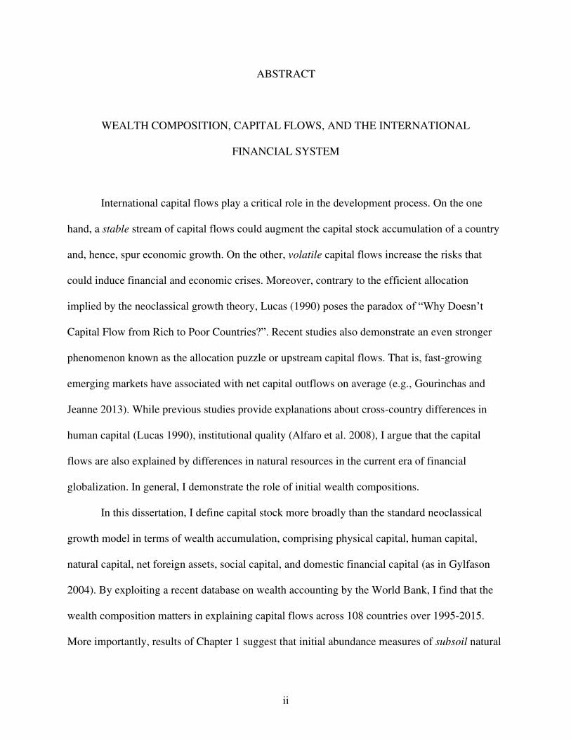
International capital flows play a critical role in the development process. On the one

hand, a stable stream of capital flows could augment the capital stock accumulation of a country

and, hence, spur economic growth. On the other, volatile capital flows increase the risks that

could induce financial and economic crises. Moreover, contrary to the efficient allocation

implied by the neoclassical growth theory, Lucas (1990) poses the paradox of “Why Doesn’t

Capital Flow from Rich to Poor Countries?”. Recent studies also demonstrate an even stronger

phenomenon known as the allocation puzzle or upstream capital flows. That is, fast-growing

emerging markets have associated with net capital outflows on average (e.g., Gourinchas and

Jeanne 2013). While previous studies provide explanations about cross-country differences in

human capital (Lucas 1990), institutional quality (Alfaro et al. 2008), I argue that the capital

flows are also explained by differences in natural resources in the current era of financial

globalization. In general, I demonstrate the role of initial wealth compositions.

In this dissertation, I define capital stock more broadly than the standard neoclassical

growth model in terms of wealth accumulation, comprising physical capital, human capital,

natural capital, net foreign assets, social capital, and domestic financial capital (as in Gylfason

2004). By exploiting a recent database on wealth accounting by the World Bank, I find that the

wealth composition matters in explaining capital flows across 108 countries over 1995-2015.

More importantly, results of Chapter 1 suggest that initial abundance measures of subsoil natural

iii

resources and net foreign asset positions explain much of the subsequent annualized average net

capital inflows. An alternative measure of net capital inflows also suggests a stabilizing role of

the valuation effects in the international financial system. In sum, measures of wealth abundance

and net capital inflows should be considered carefully in studying the patterns of international

capital flows. Results from the typical measure suggest that capital mobility allows subsoil

resource-rich countries to invest their resource rents abroad, so they could better smooth the use

of resource windfalls. Therefore, the inclusion of natural capital emphasizes the role of economic

management in whether to channel rents toward productive investment and human capital to

industrialize the economy, or to accumulate foreign assets for exchange rates managements and

for precautionary motives due to volatile international commodity prices. It should be noted that

there is no evidence on the neoclassical allocative efficiency— the relationship between

economic growth rates and net capital inflows.

Due to the insignificant finding of the allocative efficiency, Chapters 2 and 3 extend and

modify the first chapter’s conceptual framework. Chapter 2 investigates not only international

capital flows but also some explanations for the persistent global imbalances. Using a unified

sustainable growth framework with a broad definition of total wealth, I demonstrate that there

could be specific spillover effects (or specific complementarities) rather than an overall

complementarity effect, which is simply proxied by real per capita growth rates. For instance, the

interaction between human capital and physical capital generates a positive spillover effect, as

explained by Lucas (1990). Thus, the departure from the focus on the overall complementarity to

specific complementarities and tradeoffs in capital stocks provides us with a way of testing for

13 hypotheses, motivated by the broad literature of international finance and sustainable

development. Some of these are about a human capital externality, the global saving glut

iv

argument, and negative spillover effects from natural capital on institutions and financial

development. I also test for Blecker's (2005) argument on comparative advantage in selling

financial assets and find supporting evidence. The implication of such findings implies that the

current account (CA) deficit countries with highly developed financial systems have benefited

from the current international monetary and financial system (IMFS) through the role of

valuation effects. On the other hand, financial liberalization allows subsoil-rich economies to

smooth the use of windfalls through foreign reserves accumulation. Other developing countries

with CA surpluses due to excess savings, rather than low imports, reflect the flaws in the current

IMFS.

Chapter 3 is motivated by utilizing theoretical insights from overlapping generations

(OLG) models with non-Ricardian equivalence, rather than the assumption of the infinitely lived

agent as in previous chapters. I, therefore, examine not only net total capital inflows but also

consider the distinction of private and official flows. In addition to the heterogeneities in

economies’ wealth compositions, I investigate the role of demographic structures by highlighting

the aging population phenomenon. In other words, while using the unified sustainable growth

framework with a broad definition of wealth, I distinguish between private and official capital

flows, and between the relative ratios of young and old groups to the working-age population.

All these factors relate to capital flow movements through their effects on saving-investment

decisions. Overall findings support the adoption of OLG with non-Ricardian equivalence models

in analyzing aggregated and disaggregated capital flows. Also, the inclusion of demographic

factors seems to correct for the omitted variable bias. Moreover, cross-country differences in

initial wealth compositions are of great importance for different types of disaggregated capital

flows, and so policy implications differ accordingly.

v

ACKNOWLEDGMENTS

First and foremost, I praise the Almighty God for granting me the blessings, strength, and

success in pursuing such worthy endeavors of completing my graduate studies and writing this

dissertation. Also, I am extremely grateful to my parents, brothers, and sisters for their

tremendous support and love. Unfortunately, my deepest regret is that my beloved father is no

longer alive to share with us the joy of this achievement. May Allah rest his soul in peace!

It has been quite a long journey, particularly after receiving my bachelor’s degree from

King Saud University and working at the Saudi Arabian Monetary Authority since 2009. I

cannot thank enough those who had encouraged and supported my decisions to first pursue my

masters’ degree at the University of Illinois and then to acquire two years of work experience

before starting my doctorate at Colorado State University. Furthermore, I would like to express

my thanks and appreciation to my employer and sponsor for funding my educational expenses.

Besides, there are many people deserve special mentions and thanks, particularly, for their efforts

regarding this dissertation.

Since my second year in the Ph.D. program, specifically while taking a course on

development macroeconomics, Professor Ramaa Vasudevan has been providing me with

academic and expert guidance, encouragement, and continuous feedback. Besides the

development macroeconomics, she taught me a well-structured course in international finance.

Both of which reflect our research interests that I have pursued in this dissertation. I am highly

indebted to her for being such a wonderful adviser. She has helped me to develop my research

skills and critical thinking by providing an intellectually stimulating environment and debating

ideas during our research meetings. Also, I would like to express my deepest gratitude to my

vi

committee members Professor Alexandra Bernasek, Elissa Braunstein, and Stephen Koontz for

their helpful comments and suggestions. Besides their role in the committee, they have provided

me with academic guidance and taught me well-structured courses. I am truly honored to work

with all of them toward this dissertation.

Apart from my committee members, I am grateful to other faculty members in the

department, particularly those who taught me related courses which improved my research skills

and provided helpful feedback to earlier drafts of these dissertation chapters. Due to space

limitations, I would have to mention only some of them. First, since my dissertation utilizes

insights from the broad literature of sustainable macroeconomic development, I am highly

indebted to Professor Edward Barbier who introduced me to that branch of the literature and

influenced the way I conduct economic research. Furthermore, I thank Professor Stephan Weiler

for working closely with me when I started working on my dissertation. He shared great efforts

with my advisor when I was deciding the theme of my dissertation and writing the first chapter.

Also, I could not thank enough Professor Steven Pressman for his continuous guidance and

encouragement since my first semester. Moreover, I would like to thank Professors Daniele

Tavani and Sammy Zahran for their extremely helpful courses that helped me to conduct my

research.

Besides, I am so grateful to the organizers, discussants, and participants of the

conferences, seminars, and workshops where I have presented my research. My appreciations go

to those who provided me with helpful comments during the following events: the 45th and

46thAnnual Conferences of the Eastern Economic Association (New York City, 2019; Boston,

2020). The Western Graduate Student Workshop (University of Utah, 2018) and the CSU

vii

Economics Department Seminar Series (February and December 2019). Professor Aleksandr

Gevorkyan deserves special thanks for his invaluable support and insightful suggestions.

In addition, my appreciation and gratitude go to my colleagues at CSU Department of

economics for our enjoyable and hard-working years during our coursework, for their

friendships, and their helpful discussion and comments on my dissertation. Among the many, I

thank Yeva Aleksanyan, Young Hwayoung, Arpan Ganguly, Saud Altamimi, Anil Bolukoglu,

Abdullah Algarini, Ashish Sedai, Wisnu Nugroho, and Fatih Kirsanli.

There are also many people deserve special thanks for being inspirational professors and

mentors, and for being wonderful classmates, and coworkers. Regarding my master’s and

bachelor’s degrees, my thanks first go to Professors Werner Baer, Ali Toossi, Daniel Dias,

Ayman Hendy, and Ahmed Alrajhi. My deepest regret is that Professor Baer is no longer alive to

read and share his thoughts on this dissertation. Besides, I thank my best study group for our

challenging although enjoyable long hours that we spent in the libraries of the University of

Illinois at Urbana-Champaign. Thank you to Abdulelah Alrasheedy, Mauricio Cárdenas, Miguel

Sarmiento, Parfait Gasana. Furthermore, my sincere gratitude goes to my gentle roommate and

brother Zohair Bokhari, along with not only his but also my beloved family in Chicago. Finally, I

gratefully acknowledge the guidance, support, and professional experience of my coworkers,

especially during 2013-2015. Among the many, I thank Ahmed Alkholifely, Ibrahim Alali,

Mohammed Alabdullah, Faheed Alshammari, Abdulrahman Alqahtani, Gebreen Algebreen,

Waleed Alzahrani, Ryadh Alkhareif, Sultan Altowaim, and Salah Alsayaary.

viii

DEDICATION

To my mother, and the memories of my adored father.

ix

TABLE OF CONTENTS

ABSTRACT .................................................................................................................................... ii

ACKNOWLEDGMENTS .............................................................................................................. v

DEDICATION ............................................................................................................................. viii

Chapter 1 ......................................................................................................................................... 1

Wealth Composition, Valuation Effect, and Upstream Capital Flows ........................................... 1

Introduction ...................................................................................................................... 1

Wealth and Capital Flows: Measurements and Issues ..................................................... 7

1.2.1 Importance of Wealth Composition .......................................................................... 7

1.2.2 Alternative Measures of Net Capital Inflows ........................................................... 9

Literature Review ........................................................................................................... 13

Conceptual Framework and Correlations ....................................................................... 20

1.4.1 Conceptual Framework ........................................................................................... 20

1.4.2 Preliminary Unconditional Correlations ................................................................. 26

Data and Empirical Approach ........................................................................................ 32

1.5.1 Data Sources and Summary Statistics..................................................................... 32

1.5.2 Empirical Approach ................................................................................................ 36

1.5.3 Robustness Checks.................................................................................................. 38

Results ............................................................................................................................ 39

1.6.1 Regression Estimates .............................................................................................. 39

1.6.2 Robustness Check Results ...................................................................................... 43

Discussion and Conclusion ............................................................................................ 54

Chapter 2 ....................................................................................................................................... 59

International Capital Movements and Global Imbalances: The Role of Complementarities and

Tradeoffs in Capital Stocks ........................................................................................................... 59

Introduction .................................................................................................................... 59

Specific Complementarities and Tradeoffs .................................................................... 63

Data and Empirical Approach ........................................................................................ 69

2.3.1 Data Sources ........................................................................................................... 69

2.3.2 Econometric Approach ........................................................................................... 70

x

2.3.3 Descriptive Statistics ............................................................................................... 72

Diagnoses and Empirical Results ................................................................................... 73

2.4.1 Human Capital Externality ..................................................................................... 73

2.4.2 Comparative Advantage in Financial Assets .......................................................... 75

2.4.3 Global Saving Glut ................................................................................................. 80

2.4.4 Natural Resources Crowd Out Institutions ............................................................ 83

2.4.5 Natural Resource Curse in Finance......................................................................... 85

2.4.6 Results of Other Hypotheses ................................................................................... 88

Summary ........................................................................................................................ 92

Discussion and Conclusion ............................................................................................ 93

Chapter 3 ....................................................................................................................................... 97

International Capital Flows: Heterogeneities in Investor Types and in Countries’ Wealth Compositions and Demographic Structures.................................................................................. 97

Introduction .................................................................................................................... 97

Theoretical Predictions and Issues ................................................................................. 99

Data Sources and Empirical Approach ........................................................................ 104

Total Capital Flows ...................................................................................................... 106

Disaggregated Capital Flows ....................................................................................... 109

3.5.1 Private versus Official........................................................................................... 109

3.5.2 The Decomposition of Official Flows .................................................................. 117

3.5.3 The Decomposition of Private Flows ................................................................... 120

Discussion and Conclusion .......................................................................................... 127

References ................................................................................................................................... 129

Appendix A: Appendix to Chapter 1 .......................................................................................... 139

Appendix B: Appendix to Chapter 2 .......................................................................................... 150

Appendix C: Appendix to Chapter 3 .......................................................................................... 154

1

Chapter 1

Wealth Composition, Valuation Effect, and Upstream

Capital Flows

Introduction

A stable stream of foreign capital flows plays a critical role in the development process

by augmenting capital stock accumulation and sustaining the current account deficits of a

country. On the one hand, standard neoclassical theory predicts that returns to capital should be

higher in poor countries, in terms of capital-labor ratio, and hence international capital should

flow in to exploit such high returns.1 On the other hand, Lucas (1990) observes a puzzle that very

little capital flows into poor countries, and Gourinchas and Jeanne (2013) find an allocation

puzzle that fast-growing emerging markets and developing economies (EMDEs) have associated

with net capital outflows. In a few words, the allocation puzzle is the Lucas puzzle but in first

differences (gross versus net inflows, and income levels versus growth rates). Surprisingly,

cross-country differences in natural resources have been neglected in the empirical literature of

global capital allocation although there is a wide literature on the natural resource-growth nexus.

Primary goods exporting countries could be a major underlying source of the upstream capital

flows due to their economic structure and the Dutch disease effects. Therefore, I aim to

investigate the role of initial wealth composition on the medium- to long-term capital flows,

while revisiting the neoclassical allocative efficiency hypothesis across 108 countries over 1995-

2015. Wealth is defined more broadly to include net foreign assets, produced capital, human

capital, natural capital, social capital, and domestic financial capital (Gylfason 2004).

1 This is due to the law of diminishing returns— a decreasing marginal productivity of capital.

2

Accordingly, I take advantage of a recently released dataset on wealth accounts by the World

Bank, supplemented by proxies for the last two types of capital stocks. Moreover, I will consider

the role of valuation effects in studying capital movement patterns, as emphasized by recent

literature (e.g., Lane and Milesi-Ferretti 2017, 2007; Gourinchas and Rey 2015).

First, the literature on capital flows adopts the view from growth accounting literature

that cross-country differences in output growth mainly stem from differences in their total factor

productivity (TFP). It implies that fast-growing economies would invest more and associate with

higher returns to capital, so they should attract more foreign capital inflows. Nevertheless, data

on actual capital flows show the opposite pattern to what the theory predicts. Related studies,

therefore, modify some assumptions of the neoclassical growth model (NGM) and/or incorporate

other factors to provide some explanations. For instance, Lucas (1990) asserts that the answer to

the puzzle is about cross-country differences in human capital, rather than expropriation risks.

Hence, he illustrates a model in which human skills enter an aggregate homogeneous production

function as a positive externality to ensure sustained growth only in advanced countries.

Surprisingly, the recent few decades show that EMDEs have relaxed restrictions on foreign

investment but, unexpectedly, this has been associated with relatively higher growth rates and

greater net capital outflows. Consequently, if the answer is not about human capital or even

capital mobility, what could be the answer? Alfaro, Kalemli-Ozcan, and Volosovych (2008)

investigate empirically the Lucas Paradox and conclude that the answer is all about institutions,

contrasting with the Lucas argument on human capital. Yet, the role of natural resources has

been neglected in such empirical studies, so the current study aims to fill this gap among other

considerations.

3

Although some authors provide a set of possible explanations such as the Dutch disease

effects (e.g., Prasad, Rajan, and Subramanian 2007), natural resources do not appear in their

empirical models of capital flows. First, booms in commodity prices could lead to exchange rates

appreciation and factor movement toward resource sectors and hence the growth-inducing

industrial sector could shrink over time. Second, during busts, such countries would face difficult

times of large currency depreciation and debt crises especially if there are no accumulated

foreign reserves that help them to better manage volatility. Moreover, the Permanent Income

Hypothesis (PIH) is interpreted in the empirical literature of capital flows in contrast to the

literature of natural resources. For instance, Gourinchas and Jeanne (2013) assert that the

evidence of the allocation puzzle contradicts the implication of PIH— growing economies

should invest and borrow more due to their expected high growth rates. In other words, real-

world data show a puzzling behavior that highly growing economies are positively correlated

with net savings, while the PIH suggests that they should associate with net investment based on

the interpretation of Gourinchas and Jeanne. However, the role of natural resources is

completely neglected in such empirical studies on capital flows. With exhaustible natural

resources, however, I argue that the PIH should be interpreted the other way around. That is,

resource-rich countries should save more during booms to better manage their economies during

busts. In sum, previous studies on capital flows provide a set of explanations to explain the Lucas

Paradox and/or the allocation puzzle (known also as the upstream capital flows). Such

explanations could be categorized into two broad groups as follows: 1) differences in factor

supply endowments (mainly physical and external financial positions), and 2) differences in

productivity growth. Unfortunately, such studies do not specifically control for cross-country

differences in the abundance of natural resources that could drive the upstream capital flows.

4

Besides, another issue is the difficulty of constructing a direct stock measure of human

capital. In previous studies, human capital is argued to be implicitly captured in TFP as in

Gourinchas and Jeanne (2013), or generally by using some proxies as average years of schooling.

First, since the mid-1980s, the World Bank has noticed that the GDP of resource-rich countries

could be inflated, reflecting liquidation of natural resources rather than productivity

improvement. Fortunately, Lange, Wodon, and Carey (2018), from the World Bank, have

constructed a dataset on wealth accounts for 141 countries over 1995-2014. They emphasize that

cross-country economic comparisons should focus not only on income but also on wealth levels.

Among other estimate improvements, human capital is measured in a stock unit for the first time,

using over 1500 global household earnings’ surveys. Interestingly, their data show that the share

of both human and natural capital assets accounts for about 70 percent of wealth in most

countries in 2014.2 While the former is higher in advanced countries, the latter is higher in less

developed countries. Thus, exploiting this recently released data on wealth accounts could help

for a better understanding of international capital flows.

In this study, therefore, I attempt to answer the following questions:

• Does the wealth composition matter in explaining the upstream capital flows?

• Does the efficient allocation hypothesis still hold true with the broad wealth

definition?

• Would decomposing natural capital into the subsoil and non-subsoil natural capital

make a difference in explaining international capital flows?

• Do valuation effects matter in the current international financial system?

2 Refer to Table 1.1.

5

To do so, I will investigate the role of cross-country differences in wealth components

and real per capita growth in explaining the pattern of capital flow, all in per capita units.

Besides the typical measure of net capital inflows, I also consider measures of net capital inflows

that incorporate official aid flows and valuation effects. In addition, the current study covers 108

countries over 1995-2015, and the reason behind choosing this period is twofold. First, I attempt

to explain medium- to long-term movements of capital flows and, hence, I must include as many

years as possible while data on wealth starts in 1995. Second, this period is characterized by

financial globalization— more openness to foreign capital flows, financialization— a greater role

of financial activity on economic outcomes, volatile global commodity prices. Our main prior

expectation is that natural capital (especially, subsoil types that include energy, minerals, and

metals) plays an important role in explaining the upstream capital flows. To the best of my

knowledge, this is the first paper that incorporates the role of cross-country differences in initial

wealth composition to investigate international capital flows movements in a unified framework,

using the best available estimates of total wealth.

An overview of the main findings suggests the importance of the measure choice of the

net (total) capital inflows, differences in the initial abundance of natural capital as decomposed

into the subsoil and non-subsoil types, as well as net foreign assets and human capital. First, the

introduction of natural capital allows for the role of economic policy, unlike the standard

neoclassical model. Policymakers in EMDEs could decide the pace of depleting the natural

resources and hence affect the GDP level and growth (through liquidation not productive

investment) as well as the scale of capital movements when they mitigate the Dutch disease

effects. While the aggregate natural capital does not matter, its decomposition into subsoil and

non-subsoil resources helps in explaining international capital flows. Subsoil-exporting countries

6

are known to enjoy relatively higher windfalls. Second, there are three motivated measures of net

capital inflows that I discuss in section 2, and interestingly, I find that once I incorporate

valuation effects, results alter, especially with regard to the global imbalances evidence. Overall,

findings from the typical measure show evidence on persistent global imbalances, as countries

with initial CA surpluses (or a positive external financial position) have continued to have CA

surpluses on average. More importantly, findings suggest that countries with a greater initial

abundance of subsoil, rather than non-subsoil, natural capital are associated, on average, with

subsequent annualized averages of net total capital outflows during 1996-2015. That is, subsoil

natural assets seem to drive the upstream capital flows, whereas the reverse holds true for non-

subsoil natural resources (i.e., agricultural land, pastureland, forests, and protected areas). This

could imply that resource-rich countries have used their natural resource rents to accumulate

foreign assets. Thus, they seem to follow the PIH implication that these countries attempt to

smooth the use of resource windfalls overtime. In other words, resource-rich countries save more

during resource temporary windfalls/rents to dampen the effects of potential future shocks or

when they run out of resources. Besides, EMDEs have experienced economic and financial

crises due to fickle capital flows, so reserves act as a buffer during financial stress. Furthermore,

most EMDEs adopts fixed-to-less-flexible exchange rate regimes, which require foreign

exchange interventions using accumulated foreign reserves. The main implication of this study,

therefore, suggests that there is a greater role of the developmental states in utilizing resources

and using the exchange rate as an effective tool within a well-targeted industrial policy.

Countries with greater subsoil assets should improve their macroeconomic management to

achieve sustainable high growth performance.

7

The remainder of the paper is structured as follows. The next section demonstrates the

importance of wealth composition across countries and alternative measures of net (total) capital

inflows, and then sheds light on some caveats. Section 1.3 reviews the related literature. Section

1.4 develops a conceptual framework in order to make prior hypotheses and presents preliminary

unconditional correlations. Section 1.5 covers data sources, summary statistics, and an empirical

approach with some challenges. Section 1.6 reports regression results and runs a battery of

robustness checks. Section 1.7 discusses major findings along with their policy implications, and

then concludes.

Wealth and Capital Flows: Measurements and Issues

1.2.1 Importance of Wealth Composition

Since the mid-1980s, the World Bank has continued improving welfare accounting

measures because of the belief that the GDP of natural resource-rich countries is inflated due to

the liquidation of resources. The GDP measure does not reflect actual productivity gain,

especially for cross-country comparison. Recently, Lange, Wodon, and Carey (2018), from the

World Bank, construct estimates of total wealth (W). They define wealth as the sum of produced

capital and urban land (KP), net foreign assets (NFA or KF), human capital (KH), and natural

capital (KN). W = KP + KF + KH + KN (1.1)

Table 1.1 shows the share of each capital type in total wealth across country groups,

based on real per capita income in 2014. Human capital and natural capital together account for

more than 70 percent of the wealth in all country groups, where the former is relatively higher in

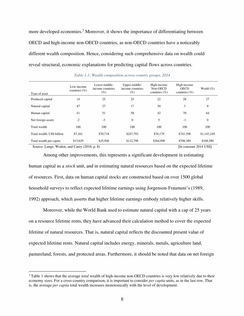
8

more developed economies.3 Moreover, it shows the importance of differentiating between

OECD and high-income non-OECD countries, as non-OECD countries have a noticeably

different wealth composition. Hence, considering such comprehensive data on wealth could

reveal structural, economic explanations for predicting capital flows across countries.

Table 1.1: Wealth composition across country groups, 2014

Type of asset

Low-income countries (%)

Lower-middle- income countries

(%)

Upper-middle- income countries

(%)

High-income Non-OECD

countries (%)

High-income OECD

countries (%) World (%)

Produced capital 14 25 25 22 28 27

Natural capital 47 27 17 30 3 9

Human capital 41 51 58 42 70 64

Net foreign assets -2 -3 0 5 -1 0

Total wealth 100 100 100 100 100 100

Total wealth, US$ billion $7,161 $70,718 $247,793 $76,179 $741,398 $1,143,249

Total wealth per capita $13,629 $25,948 $112,798 $264,998 $708,389 $168,580

Source: Lange, Wodon, and Carey (2018, p. 8) ]In constant 2014 US$ [

Among other improvements, this represents a significant development in estimating

human capital as a stock unit, and in estimating natural resources based on the expected lifetime

of resources. First, data on human capital stocks are constructed based on over 1500 global

household surveys to reflect expected lifetime earnings using Jorgenson-Fraumeni’s (1989,

1992) approach, which asserts that higher lifetime earnings embody relatively higher skills.

Moreover, while the World Bank used to estimate natural capital with a cap of 25 years

on a resource lifetime rents, they have advanced their calculation method to cover the expected

lifetime of natural resources. That is, natural capital reflects the discounted present value of

expected lifetime rents. Natural capital includes energy, minerals, metals, agriculture land,

pastureland, forests, and protected areas. Furthermore, it should be noted that data on net foreign

3 Table 1 shows that the average total wealth of high-income non-OECD countries is very low relatively due to their economy sizes. For a cross-country comparison, it is important to consider per capita units, as in the last row. That is, the average per capita total wealth increases monotonically with the level of development.

9

assets reflect the difference between a country’s foreign assets and liabilities, which estimates are

adopted from the work of Lane and Milesi-Ferretti (2007, 2017).

Although this dataset is the most accomplished effort yet for wealth accounting, there are

some caveats. First, some important natural capital components are missing. These include

renewable energy, fish stocks, water, and ecosystem services such as land and forest degradation.

Second, the World Bank excludes social capital from this definition of wealth due to difficulties

in obtaining robust estimates (for details, refer to Lange et al. 2018). Besides, I argue that income

distributional dynamics could vary across countries and adopting the human capital stock

measure could pose concerns when used in a cross-country context. Shortly, in a cross-country

comparison I believe that the calculation method is more of how relatively cheap, rather than

skilled, workers are. In addition, Gylfason's (2004) definition of wealth is broader in which the

sixth asset type is domestic financial capital.4 Although these limitations are beyond the focus of

this paper, an attempt will be made to mitigate such issues by considering proxies for social

capital/ institutions and for domestic financial development, while exploiting the best available

estimates yet of wealth to explain international capital flow patterns during 1995-2015.

1.2.2 Alternative Measures of Net Capital Inflows

Previous empirical studies demonstrate that there is no direct, single and available

measure of net (total) capital inflows in the data, so they first motivate for that (e.g., Alfaro et al.

2014).5 Although it could be possible to sum up many variables of capital flows per type,

measurement issues and errors would arise especially across a wide set of countries. Therefore,

previous literature motivates their measures from national income and the balance of payments

4 Gylfason (2004) defines total wealth as follows: 𝑊 = 𝐾𝑃 + 𝐾𝐹 + 𝐾𝐻 + 𝐾𝑁 + 𝐾𝑆𝑜𝑐𝑖𝑎𝑙 + 𝐾𝐷𝑜𝑚𝑒𝑠𝑡𝑖𝑐 𝐹𝑖𝑛𝑎𝑛𝑐𝑖𝑎𝑙 5 Only disaggregated capital flows per types are available in the data.

10

identities. Nevertheless, I observe some discrepancies surrounding such alternative measures. To

illustrate that, I start with an overview of the typical measure used widely in the literature and

then compare it with other measures.

Starting off with the typical measure adopted in the literature, which is the reverse sign of

a country’s current account (CA), normalized by the GDP level.6 The theoretical motivation

could be shown through straightforward accounting identities. First, a country’s net national

(private and public) savings are equal to the current account balance as simplified as follows:

(𝑆 − 𝐼) + (𝑇 − 𝐺) = (𝑋 − 𝑀) = 𝐶𝐴 (1.2)

The second motivation is illustrated within the balance of payments (BOP) identity.

Empirical studies adopt this definition from the simple BOP identity, based on the 5th manual

edition by the IMF, which is as follows: 𝐵𝑂𝑃 = 𝐶𝑢𝑟𝑟𝑒𝑛𝑡 𝐴𝑐𝑐𝑜𝑢𝑛𝑡 + 𝐶𝑎𝑝𝑖𝑡𝑎𝑙 𝐴𝑐𝑐𝑜𝑢𝑛𝑡 + 𝐹𝑖𝑛𝑎𝑛𝑐𝑖𝑎𝑙 𝐴𝑐𝑐𝑜𝑢𝑛𝑡 + 𝐸𝑟𝑟𝑜𝑟𝑠 and 𝑂𝑚𝑖𝑠𝑠𝑖𝑜𝑛𝑠 = 0 𝐵𝑂𝑃 = 𝐶𝐴 + 𝐾𝐴 + 𝐹𝐴 + 𝐸𝑂 = 0 (1.3)

Due to the double-entry accounting in the BOP, the sum of all components must always

be zero. Alfaro et al. (2014) show that the KA constitutes a very negligible part, based on the

data, because this account records capital transfers and the acquisition and disposal of non-

produced, non-financial assets. Also, they illustrate that the general practice is to consider

negative (positive) values of EO as non-reported capital outflows (inflows). Therefore, equation

(1.3) is simplified to the following equation: 𝑁𝑒𝑡 𝐶𝑎𝑝𝑖𝑡𝑎𝑙 𝐼𝑛𝑓𝑙𝑜𝑤𝑠 = −𝐶𝐴 = 𝐹𝐴 + EO (1.4)

6 The scaling by GDP level helps to eliminate concerns on economy-size differences.

11

That is, reversing the sign of the CA measures the financial account, which records the

following capital flows transactions: foreign direct investment (FDI), equity and debt portfolio

investment, other investment, IMF credit, and changes in official foreign reserves. However, this

measure neglects the fact that the CA comprises not only the trade balance but also unilateral aid

transfers and investment income to national factors of production. Particularly, official aid flows

could be significant in low-income countries, helping finance their trade deficits without

receiving capital flows reported in the FA balances. Investment income could also play a critical

role especially when linking the recorded flow-unit CA balances to the stock-unit net foreign

asset (NFA) positions, in this era of financial globalization.

Accordingly, there could be two additional measures of net capital inflows. First, official

aid flows have played an important role in low-income countries. Alfaro et al. (2014) state that

“capital flows into low-productivity developing countries have largely taken the form of official

aid/debt.” (p.3) Also, there is a rich strand of the literature on the growth impact of foreign aid

flows although evidence on the growth impact is inconclusive (e.g., Rajan and Subramanian

2008). Hence, I should include aid flows, reported in CA, to the other types of capital flow,

reported in FA. The focus will be on Official Development Assistance (ODA) aid flows that

include both grants and concessional loans for humanitarian and economic development rather

than military assistance. Recall the BOP identity (B=-CA=FA=0) and note that net aid receipts

are reported with a positive sign (credit in the CA) while all other types of capital inflows are

reported with a negative sign (debit in the FA). Consequently, our second measure will be as in

equation (1.5):

𝑁𝑒𝑡 (𝑡𝑜𝑡𝑎𝑙) 𝑐𝑎𝑝𝑖𝑡𝑎𝑙 𝑖𝑛𝑓𝑙𝑜𝑤𝑠 = −𝐶𝐴 + 𝑁𝑒𝑡 𝐴𝑖𝑑 𝑅𝑒𝑐𝑒𝑖𝑝𝑡𝑠 (1.5)

12

Furthermore, the third motivated measure is emphasized by the recent literature on global

imbalances. The net foreign assets (NFA) of a country summarize not only the cumulative CA

balances over time but also reflects any valuation effects (VE) — capital gains/losses due to

asset price changes and exchange rate movements, as in equation (1.6): 𝑁𝐹𝐴(𝑇) = 𝑆𝑡𝑜𝑐𝑘 𝑜𝑓 𝐹𝑜𝑟𝑒𝑖𝑔𝑛 (𝐴𝑠𝑠𝑒𝑡𝑠 − 𝐿𝑖𝑎𝑏𝑖𝑙𝑖𝑡𝑖𝑒𝑠)(𝑇) = ∑ 𝐶𝐴(𝑡)𝑇𝑡 + 𝑉𝐸(𝑇) (1.6)

Interestingly, Gourinchas and Rey (2015) illustrate two related stylized facts. First, they

show a discrepancy between cumulative CA and NFA due to fluctuations in values of existing

assets and liabilities (or the valuation effect). They also demonstrate that while the G7 advanced

countries are the largest winners, BRICS countries have been losers in terms of the valuation

effects. Unlike CA flow units, the NFA positions are reported in a stock unit. By the stock-flow

accounting, I could use equation (1.6) to derive a flow-unit measure, which captures the CA

balance plus any changes in the values of foreign assets and liabilities of a country at a specific

year. Since the change in NFA reflects net capital outflows, I reverse the sign to capture net

capital inflows. In other words, the negative change in NFA means a change in net foreign

liabilities (NFL). Thus, the third measure of net capital inflows is simplified as in equation (1.7): 𝛥𝑁𝐹𝐿𝑡 = −𝛥𝑁𝐹𝐴𝑡 = −(𝐶𝐴𝑡 + 𝛥𝑉𝐸𝑡) (1.7)

A country with a positive value of ΔNFL implies that it attracts net capital inflows, plus

any capital losses (gains) if such value is greater (less) than that of the typical measure of

equation (1.4) in a specific year.

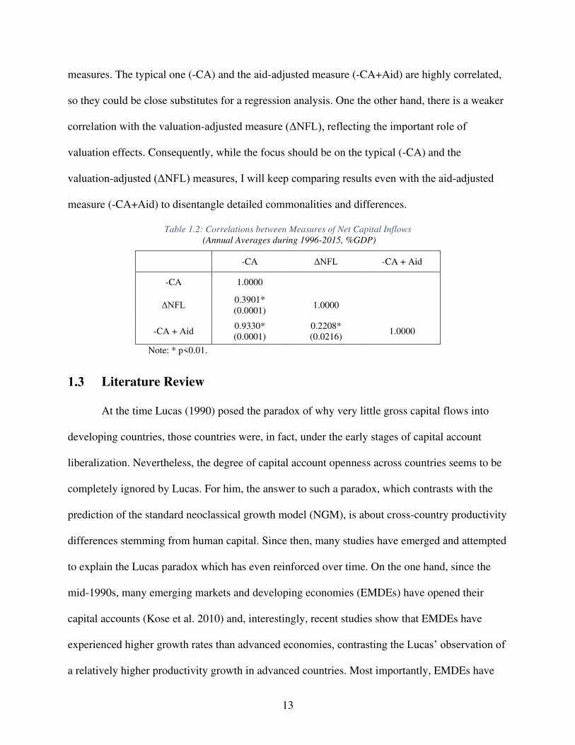
Then the question comes of whether these measures could be used as close substitutes for

the empirical regression analysis in the next sections. For comparison, I calculate annual

averages for the three measures of net capital inflow as in equations (1.4, 1.5, and 1.7),

normalized by nominal GDP, over 1996-2015. Table 1.2 reports the correlation matrix of these

13

measures. The typical one (-CA) and the aid-adjusted measure (-CA+Aid) are highly correlated,

so they could be close substitutes for a regression analysis. One the other hand, there is a weaker

correlation with the valuation-adjusted measure (ΔNFL), reflecting the important role of

valuation effects. Consequently, while the focus should be on the typical (-CA) and the

valuation-adjusted (ΔNFL) measures, I will keep comparing results even with the aid-adjusted

measure (-CA+Aid) to disentangle detailed commonalities and differences.

Table 1.2: Correlations between Measures of Net Capital Inflows

(Annual Averages during 1996-2015, %GDP)

Note: * p<0.01.

Literature Review

At the time Lucas (1990) posed the paradox of why very little gross capital flows into

developing countries, those countries were, in fact, under the early stages of capital account

liberalization. Nevertheless, the degree of capital account openness across countries seems to be

completely ignored by Lucas. For him, the answer to such a paradox, which contrasts with the

prediction of the standard neoclassical growth model (NGM), is about cross-country productivity

differences stemming from human capital. Since then, many studies have emerged and attempted

to explain the Lucas paradox which has even reinforced over time. On the one hand, since the

mid-1990s, many emerging markets and developing economies (EMDEs) have opened their

capital accounts (Kose et al. 2010) and, interestingly, recent studies show that EMDEs have

experienced higher growth rates than advanced economies, contrasting the Lucas’ observation of

a relatively higher productivity growth in advanced countries. Most importantly, EMDEs have

-CA ΔNFL -CA + Aid

-CA 1.0000

ΔNFL 0.3901* (0.0001)

1.0000

-CA + Aid 0.9330* (0.0001)

0.2208* (0.0216)

1.0000

14

experienced more of both gross capital inflows and outflows, while many fast-growing EMDEs

have even been associated with net capital outflows. This pattern of capital flows has become

known as the upstream capital flows (Alfaro, Kalemli-Ozcan, and Volosovych 2014), uphill

capital flows (Prasad, Rajan, and Subramanian 2007), and the allocation puzzle (Gourinchas and

Jeanne 2013). In sum, the allocation puzzle is the Lucas puzzle but in first differences. That is,

while the Lucas paradox is about the association between per capita income levels and gross

capital inflows, the allocation puzzle is about the association between per capita income growth

rates and net capital inflows.

Other studies provide different explanations for the Lucas Paradox and/or the allocation

puzzle such as differences in institutional quality, international capital markets frictions, and

uncertainty. Nevertheless, previous empirical studies have been neglecting the role of natural

resource abundance. Gourinchas and Jeanne (2013) find empirical evidence on the negative

association between productivity growth and net capital inflows while controlling for financial

openness along with an interaction term, which slightly dampens the allocation puzzle for only

the highly growing EMDEs. Then, they conduct a wedge analysis by distorting both savings and

investment, and conclude that the allocation puzzle is a saving puzzle. That is, EMDEs do not

face saving constraints but investment constraints. Alfaro et al. (2008) find evidence that

institutional quality is the leading factor behind the Lucas Paradox over 1970-2000. Similarly,

Papaioannou (2009) uses a large panel dataset on bilateral capital flows from banks to study the

Lucas paradox while adopting a gravity model. By exploiting two models, one of which

considers time-varying effects and the other mitigates the endogeneity concerns, his findings

suggest that institutional quality explains a large part of the Lucas Paradox. Also, an interesting

observation noted by Araujo et al. (2015) is that export revenues could substitute for capital

15

flows (p. 16). In this regard, one could think about export revenues from natural resource

liquidation and trade as a substitute for the need for capital inflows. Furthermore, Prasad et al.

(2007) discuss a set of possible explanations, including the Dutch disease effects. In fact, this is a

great support to the current study’s motivation for introducing a measure of natural resource

abundance since many oil-exporting countries, for example, have enjoyed current account

surpluses/net capital outflows due to higher prices of their exports. It should be noted that

resource-rich countries are usually excluded from the sample of most previous studies.7 On the

contrary, I address the role of natural resource differences in examining international capital

movements.

The current study is also related to the branch of the literature on institutions, natural

resources, and economic growth. One the one hand, Acemoglu, Johnson, and Robinson (2001)

argue about the fundamental role of today’s institutions on growth performance. One the other

hand, Gylfason (2004) highlights the role of natural capital which directly and adversely affects

output levels, while indirectly crowds out other types of capital, one of which is social capital —

mainly good institutions. Gylfason explains that endowments of natural resources induce rent-

seeking activity which reflects on the current institutional quality. In regard to the capital flows,

the main finding of Alfaro et al. (2008) implies that the lack of good institutions explains the

Lucas paradox. Nevertheless, their empirical analysis does not control for natural resources,

which I will consider in this study.

Since I exploit current account data, the study is also related to the branch of the literature

on savings, investment, and growth.8 All of which are also related to the permanent income

7 The main reason could be that most standard growth/capital flows empirical studies do not control for differences in natural resources and, hence, they exclude such resource-rich countries for being influential observations. 8 Recall that CA reflects the difference between a country’s savings and investment.

16

hypothesis (PIH) in which current consumption is a function of permanent income. Recall that

the neoclassical growth model maximizes the consumption level for the infinitely lived agent

subject to the intertemporal budget constraint, whereas other markets are in equilibria. Some

studies also illustrate a positive bidirectional association between savings to growth, as an

explanation for the allocation puzzle (Prasad et al. 2007; Gourinchas and Jeanne 2013).

Gourinchas and Jeanne, however, conclude that fast-growing EMDEs do not face savings

constraints but investment constraints and, therefore, the allocation puzzle is a saving puzzle—

they should invest more by borrowing against their expected future high growth rates following

the PIH. Extending this line of research, I suggest that the PIH for resource-rich EMDEs, facing

temporary resource windfalls, should use higher savings today to mitigate the effects of potential

future shocks. Boz, Cubeddu, and Obstfeld (2017) interpret the reserve accumulation by

commodity exporters as a way for smoothing the use of the commodity windfalls. Succinctly, I

suggest that the PIH is not only for smoothing consumption but also for smoothing investment in

human capital and physical capital. Further, such economies could face investment constraints

due to their dependence on exhaustible resources that adversely affect profitability and

investment in the industrial sector, which has a greater investment capacity.

Other explanations for higher saving than investment could be related to self-financing

motives and credit constraints in developing countries. Aizenman, Pinto, and Radziwill (2007)

demonstrate that international financial integration has failed to offer net sources of financing

capital to EMDEs. They show that up to 90% of investment is self-financed in EMDEs during

the 1990s. Furthermore, Buera and Shin (2017) illustrate in a joint dynamic model for TFP,

savings, and investment, with heterogeneous producers and financial frictions. When economy-

wide reforms take place and remove distortions (mainly, taxes and subsidies), TFP initially

17

increases with a larger saving response compared to a muted investment response. As a result,

the net effect of more savings than investment could explain the pattern of net capital outflows

from EMDEs.

Gourinchas and Rey (2015) discuss theoretical shortcomings in the neoclassical growth

model, mainly its underlying assumptions. These include a homogeneous aggregate production

function, a rational infinitely lived agent who maximizes the consumption path, and perfectly

mobile capital across countries. They demonstrate an open-economy model with a broader law of

motion capturing wealth, which only comprises the stock of physical capital and net foreign

assets. The model in Gourinchas and Jeanne (2013) focuses on financial wealth by empirically

controlling for initial capital abundance measures of physical capital and net external position.

Their findings show the importance of capital account openness to dampen the allocation puzzle

only for very highly growing EMDEs. Although the pattern of upstream capital flows still holds

true, faster growing economies with higher degrees of financial openness have lower ratios of net

capital outflows to GDP, relatively. Even though Gourinchas and Jeanne shed light on the

importance of financial wealth, their definition of wealth is still very narrow and neglect the

increasing role of natural resource-rich countries’ in accumulating foreign reserves and their

Sovereign Wealth Funds in the pre- and post-2008 GFC.

As discussed in the previous section, the recently available dataset on wealth accounts by

the World Bank includes two more stocks of human capital and natural capital, allowing for a

more comprehensive accounting of capital than by Gourinchas and Rey (2015). The share of

these two stocks together accounts for the lion’s share of wealth for almost all countries. Lucas’

(1988) model illustrates a positive externality from human capital on the long-run economic

18

growth. On the other hand, many studies on natural resources show negative effect from natural

resource windfalls on the long-run growth rates (e.g., Sachs and Warner 2001).

The current study is also closely related to the wide literature on the natural resource

curse that seeks to explain the relatively slower growth performance of resource-abundant

countries. Some of these explanations are as follows: trade specialization in low-productive

activity causing a deteriorating long-run term of trade; increasing the rent-seeking rather than

productive investment resulting an overall poor quality of institutions, volatile international

prices of exhaustible primary commodities deteriorate the public finance especially when having

underdeveloped financial systems, etc. (e.g., Van der Ploeg 2011; Krugman 1981; Frankel 2012;

Barbier 2007). Moreover, the Dutch disease model of Matsuyama (1992), based on an open-

economy three-sector model with international trade specialization, demonstrates a negative link

between the agricultural productivity and industrialization in the economic development process

(Barbier 2007, pp.112-119). The Dutch disease effects (or the deindustrialization process) could

be explained as in Van der Ploeg (2011, p. 377) as follows: during price booms or new

discoveries of natural resources, export revenues could induce exchange rate appreciation and,

hence, reduce the tradable non-resource sector competitiveness (i.e. the spending effect); and

workers from the productive sector get attracted by higher wages in the resource sector and/or

the non-tradable sector that have higher demand (i.e. the resource movement effect). Therefore,

the tradable non-resource sector, which is more productive, shrinks in the long run. Another

explanation of the resource curse is by Rodriguez and Sachs (1999). They illustrate that the

unsustainable high income caused by a temporary resource windfall leads to unsustainable

overconsumption and, hence, the convergence to the steady-state level occurs from above in an

overshooting neoclassical growth model. This result emphasizes the implication of the PIH in the

19

neoclassical growth model. In other words, the transitional dynamics to their steady-state level

occurs from above along the saddle path, unless there is an exogenous technological change

and/or allowing for international capital mobility. Interestingly, they acknowledge that by

relaxing the assumption of imperfect capital mobility, countries could invest in international

assets that pay permanent annuities which help them to avoid having unsustainable

overconsumption levels. Besides, while Sachs and Warner (2001) show empirical evidence that

the more resource-dependent a country was in 1970, the lower growth performance in

subsequent two decades, Manzano and Rigobon (2001) attribute the slower growth performance

of the 1980s-1990s to the debt-overhang argument. Many studies also highlight that volatile

international commodity prices adversely affect counties’ public finance, especially when the

financial system is underdeveloped (Nili and Rastad 2007; Van der Ploeg and Poelhekke 2009,

2010). Furthermore, while Gylfason (2004) discuses indirect effects from natural abundance on

growth through crowding out all other types of capital, I argue it could be also possible for

crowding in effects for some types at least. For instance, Van der Ploeg (2011) demonstrates that

diamonds account for about 40% of Botswana’s GDP but the country has managed to turn the

curse into a blessing. It has the world’s highest growth rate since 1965, associated with the

second highest expenditure on education as well as stable long-term investment exceeding 25%

of GDP, (p. 368). All in all, these studies show there are many linkages between natural

abundance, institutions, domestic financial system, NFA position which capture to some extent

the public finance. Thus, I argue that the board definition of wealth by Gylfason will help us

improve our understanding of an open-economy growth framework while studying the capital

flow movements.

20

The last two decades show that resource-rich countries had remarkable accumulations of

foreign assets, and were regarded as creditor countries on the contrary. As discussed, the

accumulation of foreign assets allows such countries to protect their exchange rates from

appreciating and helps them to smooth consumption as in the PIH. Also, such countries could

pursue an industrial policy by investment in human capital using resource rents. Accordingly, the

current study attempts to make a synthesis of two branches of the wide literature on open-

economy macroeconomics, comprising the sustainable development and capital flows. Both are

mostly discussed within the neoclassical growth theory, but the broad definition of wealth will

make the difference.

Conceptual Framework and Correlations

In this section, I begin with a conceptual framework that links theoretical insights of

different growth models to capital flow movements. Before turning to the empirical analyses, I

also present preliminary unconditional correlations to motivate the study that considers the role

of wealth composition in capital flows patterns in the recent period.

1.4.1 Conceptual Framework

This study focuses on the supply side of the economy as in the neoclassical growth model

to explain international capital flows during the convergence process. The open-economy model

illustrated in Gourinchas and Jeanne (2013) considers the accumulation of wealth, but their

definition of wealth is very limited. I attempt to extend their model by introducing a broader

definition of wealth. Gourinchas and Jeanne present an open-economy neoclassical model with

an initial abundance of both physical capital stock and net external debt stock (or NFL) in a

developing economy. They argue that productivity growth in developing countries would catch

up to some fraction of that in the US, which is considered as the technological frontier. Thus,

21

during the catching-up process, EMDEs would grow faster and attract more foreign capital

inflows due to diminishing returns to capital. This is known as the efficient allocation

hypothesis—a positive association between productivity growth and net capital inflows. Thus,

each type of capital should grow at a faster rate during the catching-up process and then at a

similar rate to the growth in income per efficiency unit in the period (T). Accordingly, they

define the initial capital abundance measure by ratios of physical capital and debt level to the

GDP level.

I extend the open-economy standard growth model by defining wealth more broadly.

While the World Bank’s definition of wealth consists of four capital types (Lange, Wodon, and

Carey 2018), a broader definition is also found in Gylfason (2004). Therefore, I will adopt the

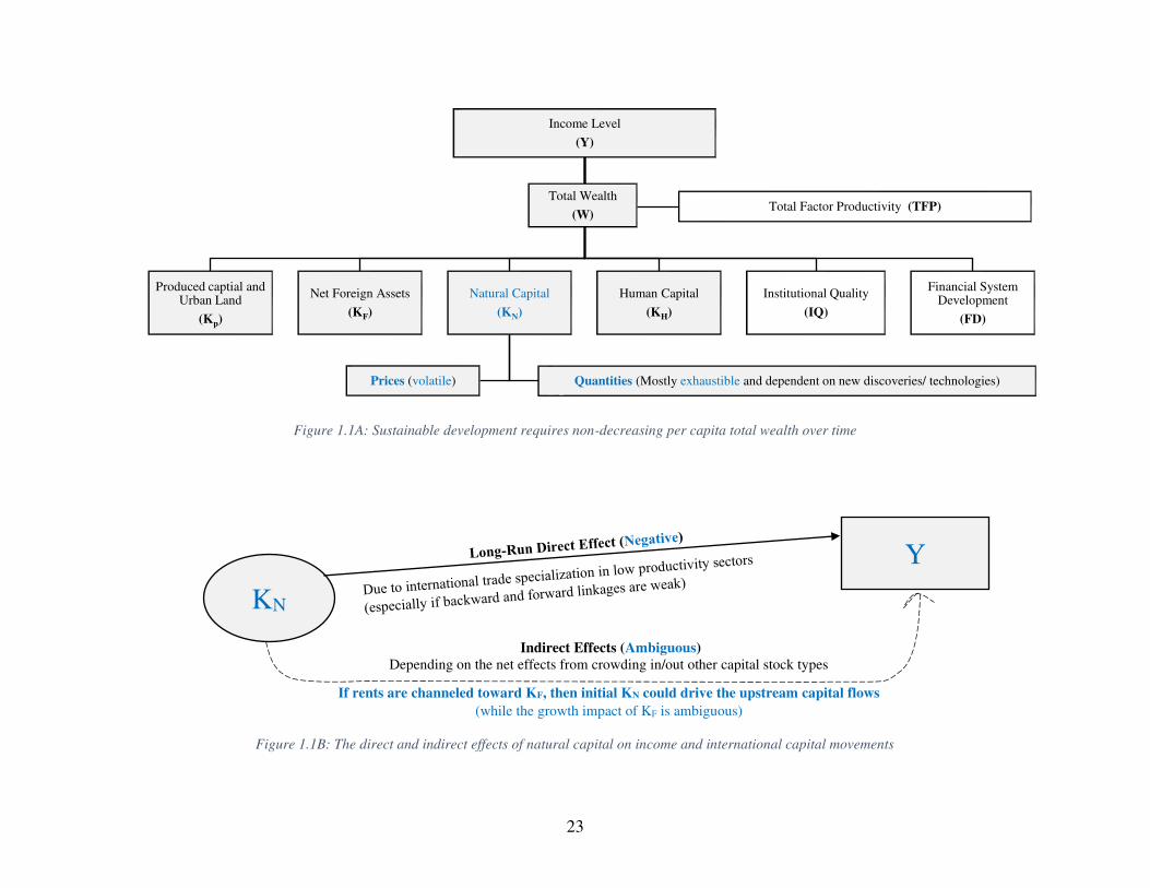
latter definition of wealth that comprises six types of capital, depicted in Figure 1.1A, so the

model (in per capita unit) becomes as follows: 𝑦𝑖𝑡 = 𝑓𝑖𝑡(𝑤𝑖𝑡)

Where: 𝑤(𝑖𝑡) = 𝑘𝑃ℎ𝑦𝑠𝑖𝑐𝑎𝑙(𝑖𝑡) + 𝑘𝑁𝐹𝐴(𝑖𝑡) + 𝑘𝐻𝑢𝑚𝑎𝑛(𝑖𝑡) + 𝑘𝑁𝑎𝑡𝑢𝑟𝑎𝑙(𝑖𝑡) + 𝑘𝑠𝑜𝑐𝑖𝑎𝑙(𝑖𝑡) + 𝑘𝐹𝑖𝑛𝑎𝑛𝑐𝑖𝑎𝑙(𝑖𝑡) (1.8)

And the subscript (it) refers to a country and year, respectively.

It would be implausible to assume all countries achieve their balanced growth paths

(BGP) by the end period of the study. Gourinchas and Jeanne (2013) assume that all countries

achieve that in 2000, the end period of their sample. Unlike the standard neoclassical growth

model, by including natural capital I can investigate the implication of natural resource

management. For Gylfason (2004), natural abundance has not only a direct negative effect on

growth but also an indirect effect through crowding out other types of capital. By contrast, there

are some successful, highly-growing, resource-abundant countries such as Botswana which were

22

able to enhance human capital, and United Arab Emirates that diversified its economy into light

manufacturing, telecommunications, finance, and tourism (Van der Ploeg 2011). These facts

show the possibility of crowding in effects, too. Accordingly, I assert that the indirect effects of

resource abundance are ambiguous. Figure 1.1B illustrates the direct and indirect effects of

natural capital abundance.

Therefore, different types of capital interact with an overall ambiguous net effect on

growth. Nevertheless, since many EMDEs are associated with fast-growing economies, I could

justify the use of the initial abundance of wealth for a better understanding of capital flow

movements. I define the abundance measures similar to Gourinchas and Jeanne (2013) but for all

types of capital stocks. Barbier (2007) discusses a debate in the sustainable development

literature about whether capital stock types could be substitutes or not. The strong sustainability

argument states that each type of capital stock must be non-decreasing, while the weak

sustainability argument states that the total wealth must be non-decreasing. Accordingly, I must

assume for the weak sustainability that is the minimum requirement of sustainable economic

growth.

In contrast to the crowding-out effects as in Gylfason (2004), I believe that in the current

era of financial globalization, policymakers in resource-abundant countries have been

accumulating NFA and allocating large shares of their annual budgets toward education, among

other things. Thus, one could argue that financial globalization has allowed policymakers in

EMDEs to channel the resource rents to higher accumulation of NFA. This might help mitigate

the Dutch disease effects by preventing the real appreciation in exchange rates, and to smooth the

23

Figure 1.1A: Sustainable development requires non-decreasing per capita total wealth over time

Figure 1.1B: The direct and indirect effects of natural capital on income and international capital movements

Income Level

(Y)

Produced captial and Urban Land

(Kp)

Net Foreign Assets

(KF)

Natural Capital

(KN)

Prices (volatile) Quantities (Mostly exhaustible and dependent on new discoveries/ technologies)

Human Capital

(KH)

Institutional Quality

(IQ)

Financial System Development

(FD)

Total Factor Productivity (TFP)Total Wealth

(W)

KN

Indirect Effects (Ambiguous)

Depending on the net effects from crowding in/out other capital stock types

If rents are channeled toward KF, then initial KN could drive the upstream capital flows

(while the growth impact of KF is ambiguous)

Y

24

use of natural resource windfalls. As discussed in the literature review section, I suggest that PIH

is not only about smoothing consumption but also smoothing investment in human capital and

physical capital. Accordingly, NFA management is crucial in which KN could crowd in KF in the

development process.

Although the above is an extended supply-side framework, the demand-side channels

could be of importance, too. Many previous studies illustrate that investment and savings have

different degrees of responsiveness to income increases. First, with habit formation in

consumption preferences, Carroll, Overland, and Weil (2000) show that an increase in income

growth can cause increased savings. Second, Buera and Shin (2017) illustrate in a joint dynamic

model that when economy-wide reforms correct for distortions (mainly, taxes and subsidies),

TFP initially increases with a larger saving response than a muted investment response.

Nevertheless, these complications are beyond the focus of the current study.

Besides, I highlight the importance of natural capital in studying international capital

flow movements. This is because per capita GDP is an erroneous measure of welfare especially

in the context of cross-country comparison. For instance, Stauffer and Lennox (1984), whose

study was commissioned by OPEC, state, “The GDP of oil-exporting states is exaggerated

because some of their income is due to the consumption of depletable oil resources and hence is

liquidation of capital, not income.’’ (as cited in Neumayer 2004, p. 1630). Consequently, the

modified model illustrated in equation (8) will allow for a better understanding of capital flow

patterns.

Rodriguez and Sachs (1999) acknowledge that the resource curse explained by the

unsustainable overconsumption argument could be avoided through investment in international

assets that pay annuities. For them, relaxing the assumption of imperfect capital mobility across

25

countries could turn the conclusion of the resource curse upside down. In addition, the policy

implications of the resource-growth relationship suggest the use of a policy mix of reserve

accumulation and industrial policy (Polterovich, Popov, and Tonis 2010). While the former helps

protect the competitiveness of the existing tradable production, the latter puts emphasis on the

manufacturing sector that generates sustainable higher growth rates. Therefore, the reserve

accumulation policy by resource-rich countries could be a major driver of the upstream capital

flows phenomenon.

My main hypothesis, hence, is that a higher initial abundance of subsoil-type natural

capital could explain much of the subsequent capital flows, as shown figure 1.B. I expect a

negative relationship between subsoil resource abundance in 1995 and the annualized average

net capital inflows over the subsequent two decades. The second hypothesis is about the global

imbalance phenomenon. Net creditor countries in 1995 tend to be associated with a subsequent

annual average of net capital outflows. In line with previous studies, I do not expect the efficient

allocation hypothesis to hold. I expect a significant and negative, rather than positive, association

between the annual averages of real per capita growth and net capital inflows (e.g., Gourinchas

and Jeanne 2013; Prasad et al. 2007).

Before turning to the empirical investigation, I should acknowledge the following

limitations. First, data availably restricts the analysis to begin in 1995. Second, per capita growth

rates and capital stocks of different types are endogenous variables. I will, therefore, consider

initial abundance measures in 1995, while investigating the allocative efficiency hypothesis over

the subsequent annual averages during 1996-2015.

26

1.4.2 Preliminary Unconditional Correlations

Before 1995, EMDEs were still under the progress of capital account liberalization, as

discussed in previous sections, and have been associated with different degrees of openness. In

addition, EMDEs have experienced relatively high growth performance during the last few

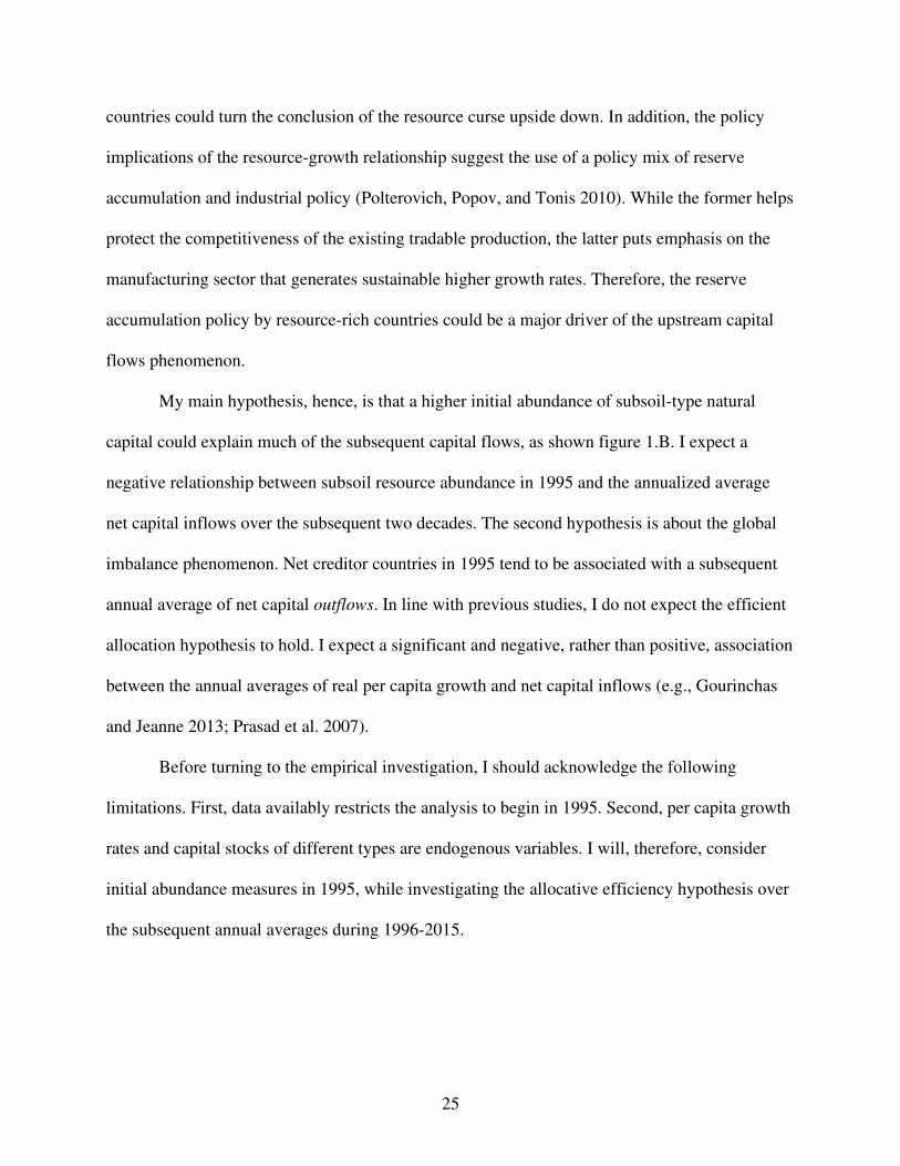
decades. Figure 1.2 shows that less developed economies, in terms of per capita income, were

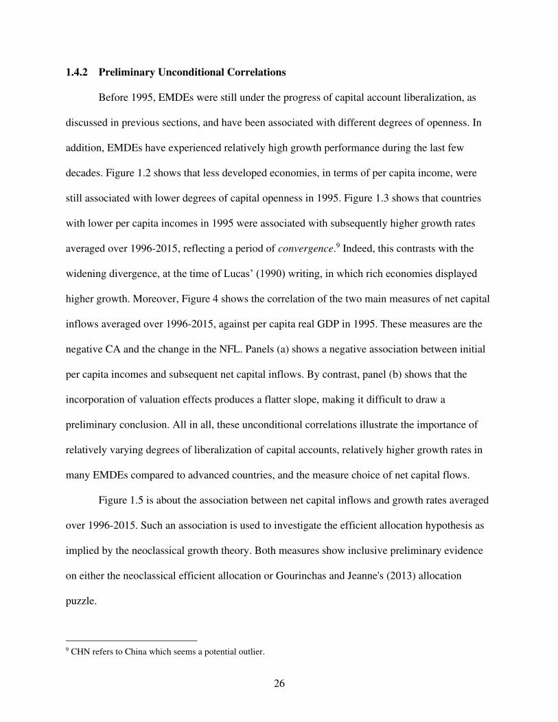
still associated with lower degrees of capital openness in 1995. Figure 1.3 shows that countries

with lower per capita incomes in 1995 were associated with subsequently higher growth rates

averaged over 1996-2015, reflecting a period of convergence.9 Indeed, this contrasts with the

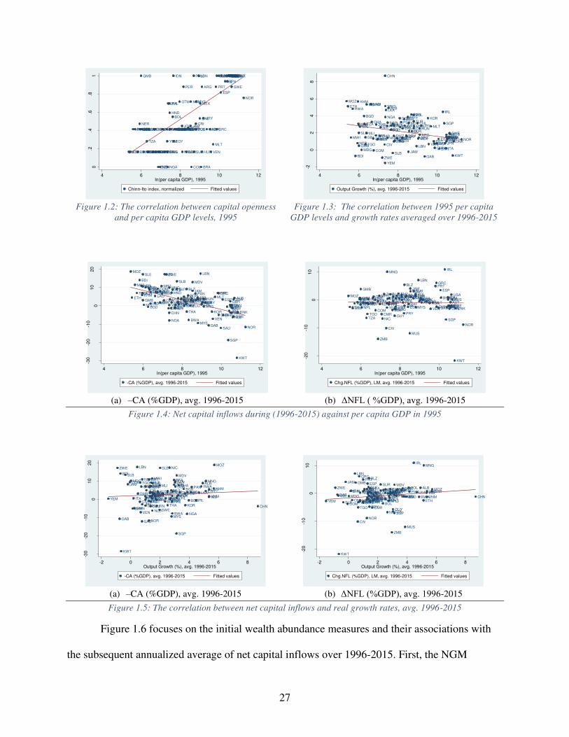
widening divergence, at the time of Lucas’ (1990) writing, in which rich economies displayed

higher growth. Moreover, Figure 4 shows the correlation of the two main measures of net capital

inflows averaged over 1996-2015, against per capita real GDP in 1995. These measures are the

negative CA and the change in the NFL. Panels (a) shows a negative association between initial

per capita incomes and subsequent net capital inflows. By contrast, panel (b) shows that the

incorporation of valuation effects produces a flatter slope, making it difficult to draw a

preliminary conclusion. All in all, these unconditional correlations illustrate the importance of

relatively varying degrees of liberalization of capital accounts, relatively higher growth rates in

many EMDEs compared to advanced countries, and the measure choice of net capital flows.

Figure 1.5 is about the association between net capital inflows and growth rates averaged

over 1996-2015. Such an association is used to investigate the efficient allocation hypothesis as

implied by the neoclassical growth theory. Both measures show inclusive preliminary evidence

on either the neoclassical efficient allocation or Gourinchas and Jeanne's (2013) allocation

puzzle.

9 CHN refers to China which seems a potential outlier.

27

Figure 1.2: The correlation between capital openness

and per capita GDP levels, 1995

Figure 1.3: The correlation between 1995 per capita

GDP levels and growth rates averaged over 1996-2015

(a) –CA (%GDP), avg. 1996-2015

(b) ΔNFL ( %GDP), avg. 1996-2015

Figure 1.4: Net capital inflows during (1996-2015) against per capita GDP in 1995

(a) –CA (%GDP), avg. 1996-2015

(b) ΔNFL (%GDP), avg. 1996-2015

Figure 1.5: The correlation between net capital inflows and real growth rates, avg. 1996-2015

Figure 1.6 focuses on the initial wealth abundance measures and their associations with

the subsequent annualized average of net capital inflows over 1996-2015. First, the NGM

ALB

ARG

AUSAUT

BDI

BEL

BFABGD

BGR

BHR

BLZ

BOL

BRA

BWA

CAN

CHL

CHN

CIVCMR COG

COL

COM

CRI

DEUDNK

DOMECU

EGY

ESP

ETH

FINFRA

GAB

GBR

GHA

GIN

GMB

GRC

GTM

GUY

HND

HUN

IDN

IND

IRL

ITA

JAMJOR

JPN

KEN

KHM KOR

KWT

LAO

LBN

LKA

MAR

MDG

MDVMEX

MLI

MLT

MNGMOZ MRT

MUSMWI

MYS

NAM

NER

NGA

NIC

NLD

NOR

NPL

OMN

PAK

PAN

PER

PHL

PNG POL

PRT

PRYRWA

SAU

SEN

SGP

SLBSLE SLV

SUR

SWE

SWZ

TGO

THATUN TUR

TZA

UGA

URY

USA

VENVNM

YEM

ZAF

ZMB

ZWE

0.2

.4.6

.81

4 6 8 10 12ln(per capita GDP), 1995

Chinn-Ito index, normalized Fitted values

ALB

ARG AUSAUT

BDI

BEL

BFA

BGDBGR

BHR

BLZ

BOL

BRA

BWA

CAN

CHL

CHN

CIV

CMR

COG

COL

COM

CRI

DEUDNK

DOM

ECU

EGY

ESP

ETH

FIN

FRA

GAB

GBR

GHA

GIN

GMBGRC

GTM

GUY

HND

HUNIDN

IND

IRL

ITAJAM

JORJPN

KEN

KHM

KOR

KWT

LAO

LBN

LKA

MAR

MDG

MDV

MEX

MLI

MLT

MNG

MOZ

MRT

MUS

MWI

MYSNAM

NER

NGA

NIC

NLDNOR

NPL

OMN

PAK

PAN

PERPHL

PNG

POL

PRTPRY

RWA

SAU

SEN

SGP

SLB

SLE

SLV

SURSWE

SWZ

TGO

THATUN

TURTZAUGA

URY

USA

VEN

VNM

YEM

ZAF

ZMB

ZWE

-20

24

68


Output Growth (%), avg. 1996-2015 Fitted values

ALB

ARG

AUS

AUT

BDI

BEL

BFA

BGD

BGR

BHR

BLZ

BOL

BRA

BWA

CANCHL

CHN

CIV

CMRCOG COL

COM

CRI

DEUDNK

DOM

ECUEGY

ESPETH

FIN

FRA

GAB

GBR

GHAGIN

GMB

GRC

GTM

GUYHND

HUN

IDNIND

IRLITA

JAM

JOR

JPN

KENKHM

KOR

KWT

LAO

LBN

LKAMAR

MDG

MDV

MEX

MLI

MLT

MNG

MOZ

MRT

MUS

MWI

MYS

NAM

NER

NGA

NIC

NLD

NOR

NPL

OMN

PAK

PAN

PER

PHLPNG

POL

PRT

PRY

RWA

SAU

SEN

SGP

SLB

SLE

SLV SUR

SWE

SWZ

TGO

THA

TUN TUR

TZA

UGA

URYUSA

VEN

VNMYEM

ZAF

ZMB

ZWE

-30

-20

-10

01

02

0


-CA (%GDP), avg. 1996-2015 Fitted values

ALB

ARGAUS

AUTBDIBEL

BFABGD

BGR BHR

BLZ

BOL

BRABWA

CAN

CHLCHN

CIV

CMR

COG

COL

COM

CRI

DEUDNK

DOM

ECU

EGY

ESP

ETH FIN

FRAGAB GBR

GHA

GIN

GMB

GRC

GTM

GUY

HNDHUNIDN

IND

IRL

ITA

JAM

JOR

JPNKEN

KHM

KOR

KWT

LAO

LBN

LKAMAR

MDG

MDV

MEXMLI MLT

MNG

MOZ MRT

MUS

MWI MYS

NAMNERNGA

NIC

NLD

NOR

NPL OMN

PAKPAN

PERPHL

PNG POL

PRT

PRY

RWA

SAU

SEN

SGP

SLBSLE

SLVSUR

SWESWZ

TGO

THA

TUNTUR

TZA

UGA URY

USA

VEN

VNMYEM

ZAF

ZMB

ZWE

-20

-10

01

0


Chg.NFL (%GDP), LM, avg. 1996-2015 Fitted values

ALB

ARG

AUS

AUT

BDI

BEL

BFA

BGD

BGR

BHR

BLZ

BOL

BRA

BWA

CAN CHL

CHN

CIV

CMRCOG COL

COM

CRI

DEUDNK

DOM

ECU EGY

ESPETH

FIN

FRA

GAB

GBR

GHAGIN

GMB

GRC

GTM

GUYHND

HUN

IDNIND

IRLITA

JAM

JOR

JPN

KEN KHM

KOR

KWT

LAO

LBN

LKAMAR

MDG

MDV

MEX

MLI

MLT

MNG

MOZ

MRT

MUS

MWI

MYS

NAM

NER

NGA

NIC

NLD

NOR

NPL

OMN

PAK

PAN

PER

PHLPNG

POL

PRT

PRY

RWA

SAU

SEN

SGP

SLB

SLE

SLV SUR

SWE

SWZ

TGO

THA

TUNTUR

TZA

UGA

URYUSA

VEN

VNMYEM

ZAF

ZMB

ZWE

-30

-20

-10

01

02

0

-2 0 2 4 6 8Output Growth (%), avg. 1996-2015


ALB

ARGAUS

AUTBDIBEL

BFABGD

BGRBHR

BLZ

BOL

BRABWA

CAN

CHLCHN

CIV

CMR

COG

COL

COM

CRI

DEUDNK

DOM

ECU

EGY

ESP

ETHFIN

FRAGAB GBR

GHA

GIN

GMB

GRC

GTM

GUY

HNDHUNIDN

IND

IRL

ITA

JAM

JOR

JPNKEN

KHM

KOR

KWT

LAO

LBN

LKAMAR

MDG

MDV

MEXMLI MLT

MNG

MOZMRT

MUS

MWI MYS

NAMNERNGA

NIC

NLD

NOR

NPLOMN

PAKPAN

PERPHL

PNG POL

PRT

PRY

RWA

SAU

SEN

SGP

SLBSLE

SLVSUR

SWESWZ

TGO

THA

TUNTUR

TZA

UGAURY

USA

VEN

VNMYEM

ZAF

ZMB

ZWE

-20

-10

01

0

-2 0 2 4 6 8Output Growth (%), avg. 1996-2015


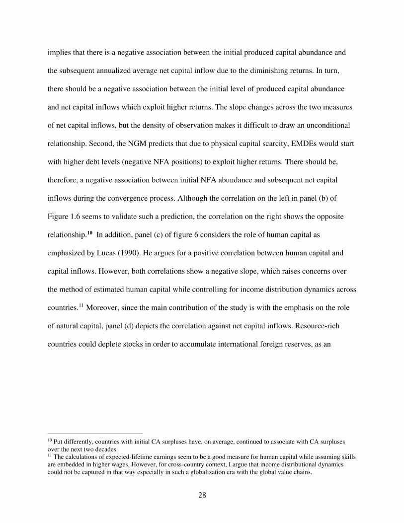
28

implies that there is a negative association between the initial produced capital abundance and

the subsequent annualized average net capital inflow due to the diminishing returns. In turn,

there should be a negative association between the initial level of produced capital abundance

and net capital inflows which exploit higher returns. The slope changes across the two measures

of net capital inflows, but the density of observation makes it difficult to draw an unconditional

relationship. Second, the NGM predicts that due to physical capital scarcity, EMDEs would start

with higher debt levels (negative NFA positions) to exploit higher returns. There should be,

therefore, a negative association between initial NFA abundance and subsequent net capital

inflows during the convergence process. Although the correlation on the left in panel (b) of

Figure 1.6 seems to validate such a prediction, the correlation on the right shows the opposite

relationship.10 In addition, panel (c) of figure 6 considers the role of human capital as

emphasized by Lucas (1990). He argues for a positive correlation between human capital and

capital inflows. However, both correlations show a negative slope, which raises concerns over

the method of estimated human capital while controlling for income distribution dynamics across

countries.11 Moreover, since the main contribution of the study is with the emphasis on the role

of natural capital, panel (d) depicts the correlation against net capital inflows. Resource-rich

countries could deplete stocks in order to accumulate international foreign reserves, as an

10 Put differently, countries with initial CA surpluses have, on average, continued to associate with CA surpluses over the next two decades. 11 The calculations of expected-lifetime earnings seem to be a good measure for human capital while assuming skills are embedded in higher wages. However, for cross-country context, I argue that income distributional dynamics could not be captured in that way especially in such a globalization era with the global value chains.

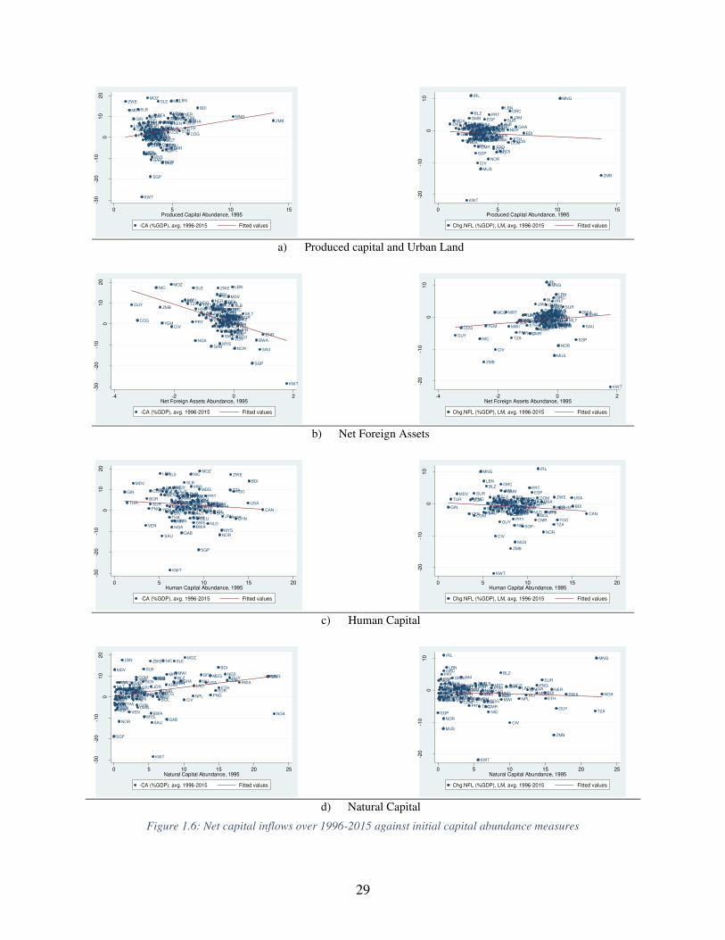
29

a) Produced capital and Urban Land

b) Net Foreign Assets

c) Human Capital

d) Natural Capital

Figure 1.6: Net capital inflows over 1996-2015 against initial capital abundance measures

ALB

ARG

AUS

AUT

BDI

BEL

BFA

BGD

BGR

BHR

BLZ

BOL

BRA

BWA

CANCHL

CHN

CIV

CMRCOGCOL

COM

CRI

DEUDNK

DOM

ECUEGY

ESPETH

FIN

FRA

GAB

GBR

GHAGIN

GMB

GRC

GTM

GUYHND

HUN

IDNIND

IRLITA

JAM

JOR

JPN

KENKHM

KOR

KWT

LAO

LBN

LKAMAR

MDG

MDV

MEX

MLI

MLT

MNG

MOZ

MRT

MUS

MWI

MYS

NAM

NER

NGA

NIC

NLD

NOR

NPL

OMN

PAK

PAN

PER

PHLPNG

POL

PRT

PRY

RWA

SAU

SEN

SGP

SLB

SLE

SLV SUR

SWE

SWZ

TGO

THA

TUNTUR

TZA

UGA

URYUSA

VEN

VNMYEM

ZAF

ZMB

ZWE

-30

-20

-10

01

02

0

0 5 10 15Produced Capital Abundance, 1995


ALB

ARGAUS

AUT BDIBEL

BFABGD

BGR BHR

BLZ

BOL

BRABWA

CAN

CHLCHN

CIV

CMR

COG

COL

COM

CRI

DEUDNK

DOM

ECU

EGY

ESP

ETHFIN

FRAGABGBR

GHA

GIN

GMB

GRC

GTM

GUY

HNDHUNIDN

IND

IRL

ITA

JAM

JOR

JPNKEN

KHM

KOR

KWT

LAO

LBN

LKAMAR

MDG

MDV

MEXMLIMLT

MNG

MOZ MRT

MUS

MWIMYS

NAM NERNGA

NIC

NLD

NOR

NPL OMN

PAKPAN

PERPHL

PNG POL

PRT

PRY

RWA

SAU

SEN

SGP

SLBSLE

SLVSUR

SWESWZ

TGO

THA

TUNTUR

TZA

UGAURY

USA

VEN

VNMYEMZAF

ZMB

ZWE

-20

-10

01

0

0 5 10 15Produced Capital Abundance, 1995


ALB

ARG

AUS

AUT

BDI

BEL

BFA

BGD

BGR

BHR

BLZ

BOL

BRA

BWA

CANCHL

CHN

CIV

CMRCOG COL

COM

CRI

DEUDNK

DOM

ECU EGY

ESPETH

FIN

FRA

GAB

GBR

GHAGIN

GMB

GRC

GTM

GUYHND

HUN

IDNIND

IRLITA

JAM

JOR

JPN

KEN KHM

KOR

KWT

LAO

LBN

LKAMAR

MDG

MDV

MEX

MLI

MLT

MNG

MOZ

MRT

MUS

MWI

MYS

NAM

NER

NGA

NIC

NLD

NOR

NPL

OMN

PAK

PAN

PER

PHLPNG

POL

PRT

PRY

RWA

SAU

SEN

SGP

SLB

SLE

SLV SUR

SWE

SWZ

TGO

THA

TUN TUR

TZA

UGA

URYUSA

VEN

VNMYEM

ZAF

ZMB

ZWE

-30

-20

-10

01

02

0

-4 -2 0 2Net Foreign Assets Abundance, 1995


ALB

ARGAUS

AUTBDIBEL

BFABGD

BGR BHR

BLZ

BOL

BRABWA

CAN

CHLCHN

CIV

CMR

COG

COL

COM

CRI

DEUDNK

DOM

ECU

EGY

ESP

ETH FIN

FRAGAB GBRGHA

GIN

GMB

GRC

GTM

GUY

HNDHUNIDN

IND

IRL

ITA

JAM

JOR

JPNKEN

KHM

KOR

KWT

LAO

LBN

LKAMAR

MDG

MDV

MEXMLI MLT

MNG

MOZ MRT

MUS

MWI MYS

NAMNERNGA

NIC

NLD

NOR

NPL OMN

PAKPAN

PERPHL

PNGPOL

PRT

PRY

RWA

SAU

SEN

SGP

SLBSLE

SLVSUR

SWE SWZ

TGO

THA

TUNTUR

TZA

UGAURY

USA

VEN

VNMYEM

ZAF

ZMB

ZWE

-20

-10

01

0

-4 -2 0 2Net Foreign Assets Abundance, 1995


ALB

ARG

AUS

AUT

BDI

BEL

BFA

BGD

BGR

BHR

BLZ

BOL

BRA

BWA

CANCHL

CHN

CIV

CMRCOG COL

COM

CRI

DEUDNK

DOM

ECUEGY

ESPETH

FIN

FRA

GAB

GBR

GHAGIN

GMB

GRC

GTM

GUYHND

HUN

IDNIND

IRLITA

JAM

JOR

JPN

KENKHM

KOR

KWT

LAO

LBN

LKAMAR

MDG

MDV

MEX

MLI

MLT

MNG

MOZ

MRT

MUS

MWI

MYS

NAM

NER

NGA

NIC

NLD

NOR

NPL

OMN

PAK

PAN

PER

PHLPNG

POL

PRT

PRY

RWA

SAU

SEN

SGP

SLB

SLE

SLVSUR

SWE

SWZ

TGO

THA

TUNTUR

TZA

UGA

URYUSA

VEN

VNMYEM

ZAF

ZMB

ZWE

-30

-20

-10

01

02

0

0 5 10 15 20Human Capital Abundance, 1995


ALB

ARGAUS

AUT BDIBEL

BFABGD

BGR BHR

BLZ

BOL

BRABWA

CAN

CHLCHN

CIV

CMR

COG

COL

COM

CRI

DEUDNK

DOM

ECU

EGY

ESP

ETHFIN

FRAGAB GBR

GHA

GIN

GMB

GRC

GTM

GUY

HNDHUN IDNIND

IRL

ITA

JAM

JOR

JPNKEN

KHM

KOR

KWT

LAO

LBN

LKAMAR

MDG

MDV

MEXMLI MLT

MNG

MOZMRT

MUS

MWI MYS

NAMNERNGA

NIC

NLD

NOR

NPLOMN

PAKPAN

PERPHL

PNG POL

PRT

PRY

RWA

SAU

SEN

SGP

SLBSLE

SLVSUR

SWESWZ

TGO

THA

TUNTUR

TZA

UGA URY

USA

VEN

VNMYEM

ZAF

ZMB

ZWE

-20

-10

01

0

0 5 10 15 20Human Capital Abundance, 1995


ALB

ARG

AUS

AUT

BDI

BEL

BFA

BGD

BGR

BHR

BLZ

BOL

BRA

BWA

CAN CHL

CHN

CIV

CMRCOGCOL

COM

CRI

DEUDNK

DOM

ECUEGY

ESPETH

FIN

FRA

GAB

GBR

GHAGIN

GMB

GRC

GTM

GUYHND

HUN

IDNIND

IRLITA

JAM

JOR

JPN

KENKHM

KOR

KWT

LAO

LBN

LKAMAR

MDG

MDV

MEX

MLI

MLT

MNG

MOZ

MRT

MUS

MWI

MYS

NAM

NER

NGA

NIC

NLD

NOR

NPL

OMN

PAK

PAN

PER

PHLPNG

POL

PRT

PRY

RWA

SAU

SEN

SGP

SLB

SLE

SLV SUR

SWE

SWZ

TGO

THA

TUNTUR

TZA

UGA

URYUSA

VEN

VNMYEM

ZAF

ZMB

ZWE

-30

-20

-10

01

02

0

0 5 10 15 20 25Natural Capital Abundance, 1995


ALB

ARGAUS

AUT BDIBEL

BFABGD

BGRBHR

BLZ

BOL

BRABWA

CAN

CHLCHN

CIV

CMR

COG

COL

COM

CRI

DEUDNK

DOM

ECU

EGY

ESP

ETHFIN

FRAGABGBR

GHA

GIN

GMB

GRC

GTM

GUY

HNDHUN IDN

IND

IRL

ITA

JAM

JOR

JPNKEN

KHM

KOR

KWT

LAO

LBN

LKAMAR

MDG

MDV

MEXMLIMLT

MNG

MOZMRT

MUS

MWIMYS

NAM NERNGA

NIC

NLD

NOR

NPLOMN

PAKPAN

PERPHL

PNGPOL

PRT

PRY

RWA

SAU

SEN

SGP

SLBSLE

SLVSUR

SWE SWZ

TGO

THA

TUNTUR

TZA

UGAURY

USA

VEN

VNMYEM

ZAF

ZMB

ZWE

-20

-10

01

0

0 5 10 15 20 25Natural Capital Abundance, 1995


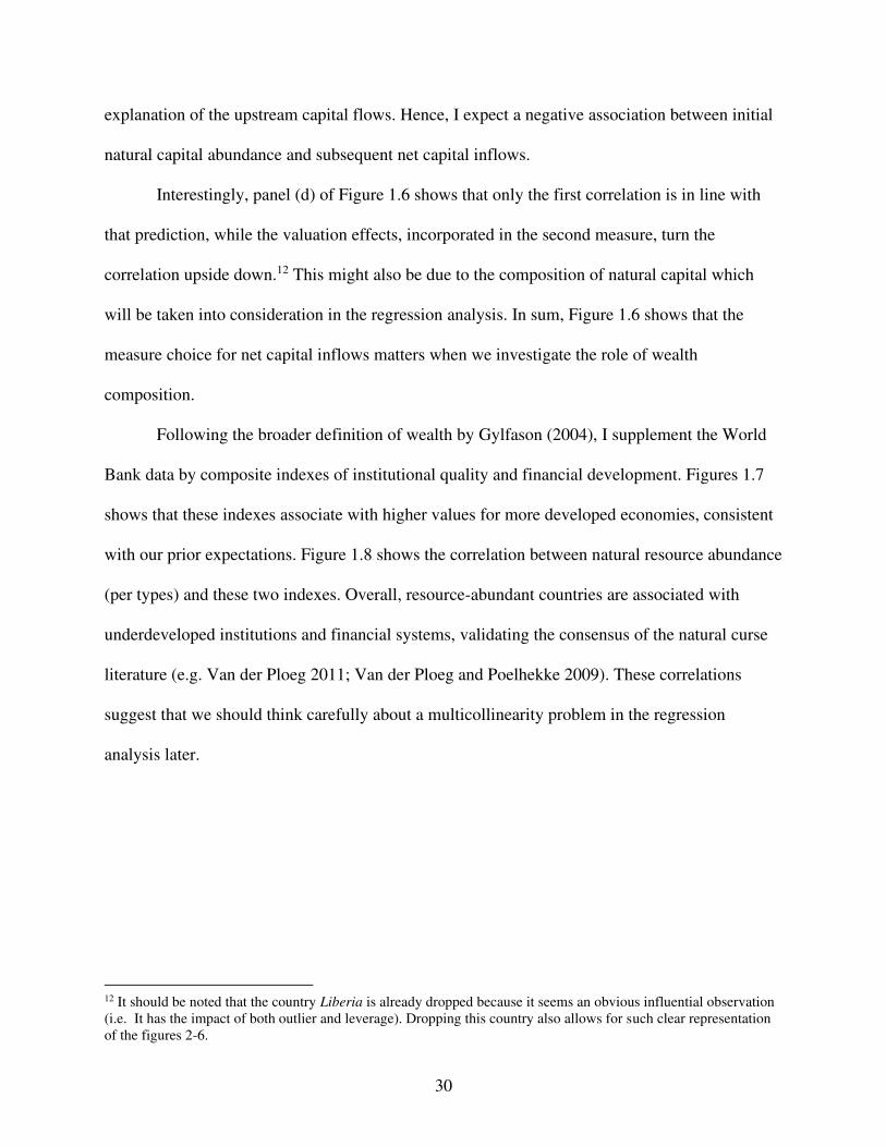
30

explanation of the upstream capital flows. Hence, I expect a negative association between initial

natural capital abundance and subsequent net capital inflows.

Interestingly, panel (d) of Figure 1.6 shows that only the first correlation is in line with

that prediction, while the valuation effects, incorporated in the second measure, turn the

correlation upside down.12 This might also be due to the composition of natural capital which

will be taken into consideration in the regression analysis. In sum, Figure 1.6 shows that the

measure choice for net capital inflows matters when we investigate the role of wealth

composition.

Following the broader definition of wealth by Gylfason (2004), I supplement the World

Bank data by composite indexes of institutional quality and financial development. Figures 1.7

shows that these indexes associate with higher values for more developed economies, consistent

with our prior expectations. Figure 1.8 shows the correlation between natural resource abundance

(per types) and these two indexes. Overall, resource-abundant countries are associated with

underdeveloped institutions and financial systems, validating the consensus of the natural curse

literature (e.g. Van der Ploeg 2011; Van der Ploeg and Poelhekke 2009). These correlations

suggest that we should think carefully about a multicollinearity problem in the regression

analysis later.

12 It should be noted that the country Liberia is already dropped because it seems an obvious influential observation (i.e. It has the impact of both outlier and leverage). Dropping this country also allows for such clear representation of the figures 2-6.

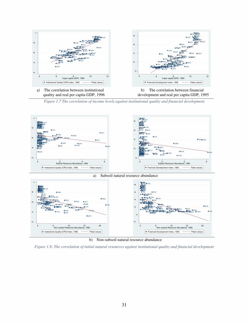
31

Figure 1.7 The correlation of income levels against institutional quality and financial development

Figure 1.8: The correlation of initial natural resources against institutional quality and financial development

a) The correlation between institutional

quality and real per capita GDP, 1996

b) The correlation between financial

development and real per capita GDP, 1995

a) Subsoil natural resource abundance

b) Non-subsoil natural resource abundance

ALB

ARG

AUSAUT

BEL

BFABGD

BGR

BHR

BOL

BRA

BWA

CAN

CHL

CHNCIV

CMR

COGCOL

CRI

DEU

DNK

DOM

ECUEGY

ESP

ETH

FIN

FRA

GAB

GBR

GHA

GIN

GMB

GRC

GTMGUY

HND

HUN

IDN

IND

IRL

ITA

JAM

JOR

JPN

KEN

KOR

KWT

LBN

LKA

MAR

MDG

MEX

MLI

MLT

MNG

MOZMWI

MYS

NAM

NER

NGA

NIC

NLDNOR

OMN

PAK

PANPER

PHL PNG

POLPRT

PRY

SAUSEN

SGP

SLE

SLVSUR

SWE

TGO

THA

TUN

TURTZA

UGA

URY

USA

VEN

VNMYEM

ZAF

ZMBZWE

.2.4

.6.8

1


Institutional Quality ICRG Index, 1996 Fitted values

ALB

ARG

AUS

AUT

BDI

BEL

BFA

BGD

BGR BHR

BLZ

BOL

BRA

BWA

CAN

CHLCHN

CIV

CMRCOG

COL

COM

CRI

DEUDNK

DOMECU

EGY

ESP

ETH

FIN

FRA

GAB

GBR

GHAGINGMB

GRC

GTMGUYHND

HUN

IDN

IND

IRLITA

JAM

JOR

JPN

KEN

KHM

KOR

KWT

LAO

LBN

LKA

MAR

MDG

MDV

MEX

MLI

MLT

MNG

MOZ MRT

MUS

MWI

MYS

NAM

NER

NGANIC

NLD

NOR

NPL

OMNPAK

PANPER

PHL

PNG

POL

PRT

PRYRWA

SAU

SEN

SGP

SLBSLE

SLV

SUR

SWE

SWZTGO

THA

TUN

TUR

TZAUGA

URY

USA

VENVNM

YEM

ZAF

ZMB

0.2

.4.6

.8


Financial Development Index, 1995 Fitted values

ALB

ARG

AUSAUTBEL

BFABGD

BGR

BHR

BOL

BRA

BWA

CAN

CHL

CHNCIV

CMR

COGCOL

CRI

DEU

DNK

DOM

ECUEGY

ESP

ETH

FIN

FRA

GAB

GBR

GHA

GIN

GMB

GRC

GTMGUY

HND

HUN

IDN

IND

IRL

ITA

JAM

JOR

JPN

KEN

KOR

KWT

LBN

LKA

MAR

MDG

MEX

MLI

MLT

MNG

MOZMWI

MYS

NAM

NER

NGA

NIC

NLDNOR

OMN

PAK

PANPER

PHL PNG

POLPRT

PRY

SAUSEN

SGP

SLE

SLVSUR

SWE

TGO

THA

TUN

TURTZA

UGA

URY

USA

VEN

VNMYEM

ZAF

ZMBZWE

.2.4

.6.8

1

0 2 4 6Subsoil Resource Abundance, 1995


ALB

ARG

AUS

AUT

BDI

BEL

BFA

BGD

BGRBHR

BLZ

BOL

BRA

BWA

CAN

CHLCHN

CIV

CMRCOG

COL

COM

CRI

DEUDNK

DOMECU

EGY

ESP

ETH

FIN

FRA

GAB

GBR

GHAGINGMB

GRC

GTMGUYHND

HUN

IDN

IND

IRLITA

JAM

JOR

JPN

KEN

KHM

KOR

KWT

LAO

LBN

LKA

MAR

MDG

MDV

MEX

MLI

MLT

MNG

MOZ MRT

MUS

MWI

MYS

NAM

NER

NGANIC

NLD

NOR

NPL

OMN

PAKPAN

PER

PHL

PNG

POL

PRT

PRYRWA

SAU

SEN

SGP

SLB

SLE

SLV

SUR

SWE

SWZTGO

THA

TUN

TUR

TZAUGA

URY

USA

VENVNM

YEM

ZAF

ZMB

0.2

.4.6

.8

0 2 4 6Subsoil Resource Abundance, 1995


ALB

ARG

AUSAUT

BEL

BFABGD

BGR

BHR

BOL

BRA

BWA

CAN

CHL

CHNCIV

CMR

COGCOL

CRI

DEU

DNK

DOM

ECUEGY

ESP

ETH

FIN

FRA

GAB

GBR

GHA

GIN

GMB

GRC

GTMGUY

HND

HUN

IDN

IND

IRL

ITA

JAM

JOR

JPN

KEN

KOR

KWT

LBN

LKA

MAR

MDG

MEX

MLI

MLT

MNG

MOZMWI

MYS

NAM

NER

NGA

NIC

NLDNOR

OMN

PAK

PANPER

PHL PNG

POLPRT

PRY

SAUSEN

SGP

SLE

SLVSUR

SWE

TGO

THA

TUN

TURTZA

UGA

URY

USA

VEN

VNMYEM

ZAF

ZMBZWE

.2.4

.6.8

1

0 5 10 15 20Non-subsoil Resource Abundance, 1995


ALB

ARG

AUS

AUT

BDI

BEL

BFA

BGD

BGRBHR

BLZ

BOL

BRA

BWA

CAN

CHL CHN

CIV

CMRCOG

COL

COM

CRI

DEUDNK

DOMECU

EGY

ESP

ETH

FIN

FRA

GAB

GBR

GHAGINGMB

GRC

GTMGUYHND

HUN

IDN

IND

IRLITA

JAM

JOR

JPN

KEN

KHM

KOR

KWT

LAO

LBN

LKA

MAR

MDG

MDV

MEX

MLI

MLT

MNG

MOZMRT

MUS

MWI

MYS

NAM

NERNGANIC

NLD

NOR

NPL

OMNPAK

PANPER

PHL

PNG

POL

PRT

PRYRWA

SAU

SEN

SGP

SLBSLE

SLV

SUR

SWE

SWZ TGO

THA

TUN

TUR

TZAUGA

URY

USA

VENVNM

YEM

ZAF

ZMB

-.2

0.2

.4.6

.8

0 5 10 15 20Non-subsoil Resource Abundance, 1995


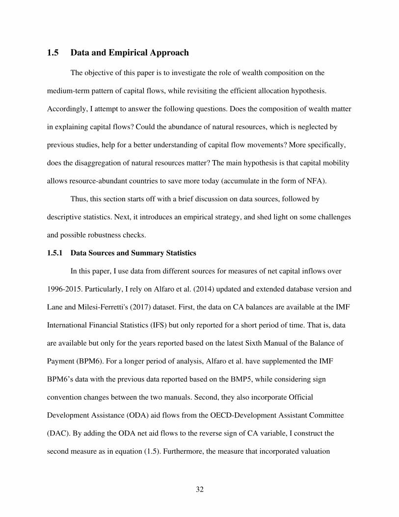
32

Data and Empirical Approach

The objective of this paper is to investigate the role of wealth composition on the

medium-term pattern of capital flows, while revisiting the efficient allocation hypothesis.

Accordingly, I attempt to answer the following questions. Does the composition of wealth matter

in explaining capital flows? Could the abundance of natural resources, which is neglected by

previous studies, help for a better understanding of capital flow movements? More specifically,

does the disaggregation of natural resources matter? The main hypothesis is that capital mobility

allows resource-abundant countries to save more today (accumulate in the form of NFA).

Thus, this section starts off with a brief discussion on data sources, followed by

descriptive statistics. Next, it introduces an empirical strategy, and shed light on some challenges

and possible robustness checks.

1.5.1 Data Sources and Summary Statistics

In this paper, I use data from different sources for measures of net capital inflows over

1996-2015. Particularly, I rely on Alfaro et al. (2014) updated and extended database version and

Lane and Milesi-Ferretti's (2017) dataset. First, the data on CA balances are available at the IMF

International Financial Statistics (IFS) but only reported for a short period of time. That is, data

are available but only for the years reported based on the latest Sixth Manual of the Balance of

Payment (BPM6). For a longer period of analysis, Alfaro et al. have supplemented the IMF

BPM6’s data with the previous data reported based on the BMP5, while considering sign

convention changes between the two manuals. Second, they also incorporate Official

Development Assistance (ODA) aid flows from the OECD-Development Assistant Committee

(DAC). By adding the ODA net aid flows to the reverse sign of CA variable, I construct the

second measure as in equation (1.5). Furthermore, the measure that incorporated valuation

33

effects, as in equation (1.7), is constructed from the data on NFA estimated by Lane and Milesi-

Ferretti (2007, 2017).

Other data sources are as follows: population and real GDP from the World Bank-World

Development Indicators (WB-WDI), sub-indicators of institutional quality are from the Political

Risk Services- International Country Risk Guide (ICRG) database, a composite index of

financial system development from Svirydzenka (2016), a de jure capital account openness index

from the updated dataset of Chinn and Ito (2006). The indexes range between zero and one, with

greater values for higher degrees of developed financial systems and openness to foreign capital

flows. Using the ICRG data, I constructed an average-weighted index for institutional quality

using these six sub-indicators: 1) voice and accountability, 2) political stability and absence of

violence, 3) government effectiveness, 4) regulatory quality, 5) rule of law, and 6) control of

corruption. Finally, and most importantly, the recently released data on wealth are from the

World Bank-Wealth Accounts (WB-WA) database.

Table 1.3 reports the descriptive statistics, while a pair-wise correlation matrix is reported

in the appendix Table C3. It should be noted this study considers economies of different sizes, so

all variables must be in per capita units. Moreover, the 1995 capital abundance measures are

defined as the per capita stock of each capital type divided by per capita GDP.13 First, and

interestingly, the sample means of the alternative measures of net capital inflows show different

signs, showing the important role of aid flows and valuation effects as discussed in section 1.2.1.

Second, data show large cross-country differences, especially for the initial natural capital

abundance ranging from a ratio of zero to 22.92.14 Furthermore, an average country in the sample

13 Since real per capita GDP data are in constant 2010 USD while wealth measures are in constant 2014USD, I adjust the base year of the former to 2014 for consistency. 14 In fact, an influential country, Liberia, is dropped from the sample because of an initial value of natural capital abundance of 72.49.

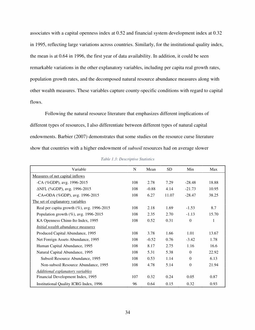
34

associates with a capital openness index at 0.52 and financial system development index at 0.32

in 1995, reflecting large variations across countries. Similarly, for the institutional quality index,

the mean is at 0.64 in 1996, the first year of data availability. In addition, it could be seen

remarkable variations in the other explanatory variables, including per capita real growth rates,

population growth rates, and the decomposed natural resource abundance measures along with

other wealth measures. These variables capture county-specific conditions with regard to capital

flows.

Following the natural resource literature that emphasizes different implications of

different types of resources, I also differentiate between different types of natural capital

endowments. Barbier (2007) demonstrates that some studies on the resource curse literature

show that countries with a higher endowment of subsoil resources had on average slower

Table 1.3: Descriptive Statistics

Variable N Mean SD Min Max

Measures of net capital inflows

-CA (%GDP), avg. 1996-2015 108 2.78 7.29 -28.48 18.88

ΔNFL (%GDP), avg. 1996-2015 108 -0.88 4.14 -21.73 10.95

-CA+ODA (%GDP), avg. 1996-2015 108 6.27 11.07 -28.47 38.25

The set of explanatory variables

Real per capita growth (%), avg. 1996-2015 108 2.18 1.69 -1.53 8.7

Population growth (%), avg. 1996-2015 108 2.35 2.70 -1.13 15.70

KA Openness Chinn-Ito Index, 1995 108 0.52 0.31 0 1

Initial wealth abundance measures

Produced Capital Abundance, 1995 108 3.78 1.66 1.01 13.67

Net Foreign Assets Abundance, 1995 108 -0.52 0.76 -3.42 1.78

Human Capital Abundance, 1995 108 8.17 2.75 1.16 16.6

Natural Capital Abundance, 1995 108 5.31 5.38 0 22.92

Subsoil Resource Abundance, 1995 108 0.53 1.14 0 6.13

Non-subsoil Resource Abundance, 1995 108 4.78 5.14 0 21.94

Additional explanatory variables

Financial Development Index, 1995 107 0.32 0.24 0.05 0.87

Institutional Quality ICRG Index, 1996 96 0.64 0.15 0.32 0.93

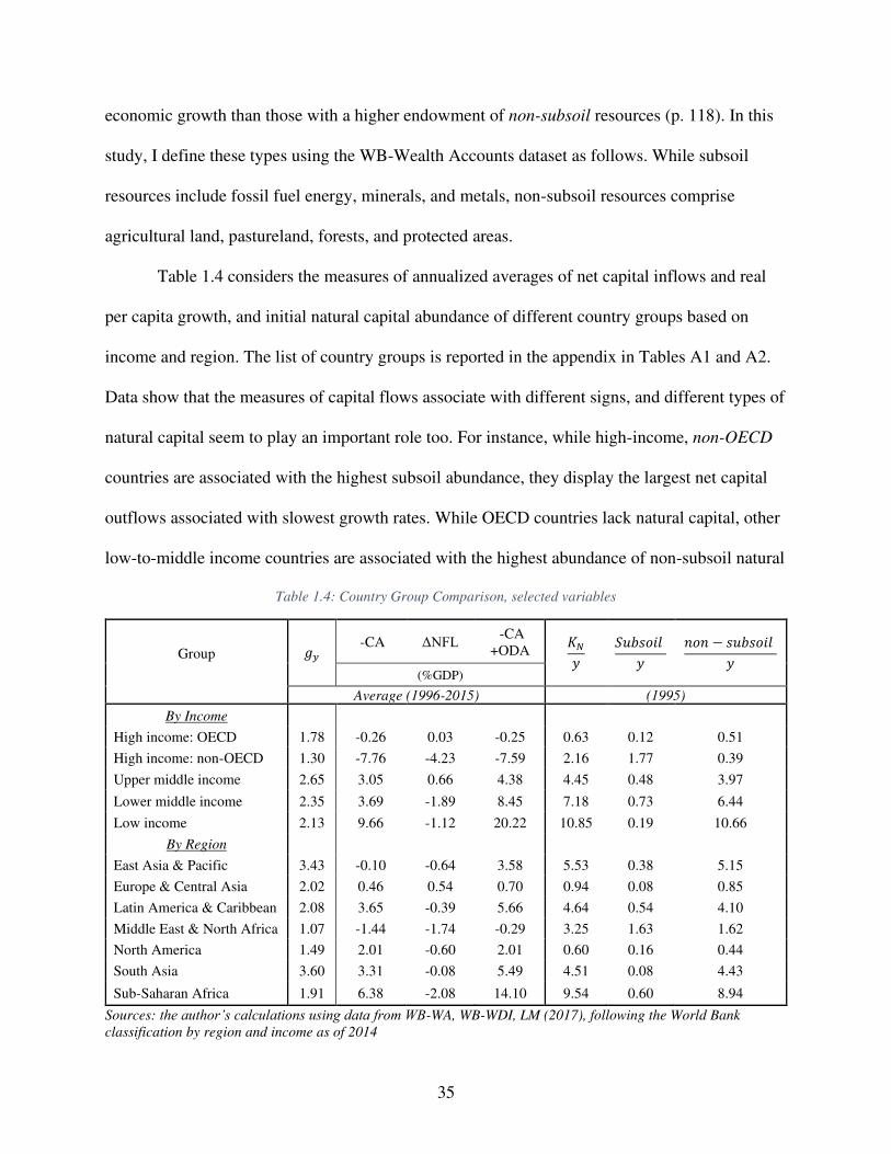
35

economic growth than those with a higher endowment of non-subsoil resources (p. 118). In this

study, I define these types using the WB-Wealth Accounts dataset as follows. While subsoil

resources include fossil fuel energy, minerals, and metals, non-subsoil resources comprise

agricultural land, pastureland, forests, and protected areas.

Table 1.4 considers the measures of annualized averages of net capital inflows and real

per capita growth, and initial natural capital abundance of different country groups based on

income and region. The list of country groups is reported in the appendix in Tables A1 and A2.

Data show that the measures of capital flows associate with different signs, and different types of

natural capital seem to play an important role too. For instance, while high-income, non-OECD

countries are associated with the highest subsoil abundance, they display the largest net capital

outflows associated with slowest growth rates. While OECD countries lack natural capital, other

low-to-middle income countries are associated with the highest abundance of non-subsoil natural

Table 1.4: Country Group Comparison, selected variables

Group 𝑔𝑦 -CA ΔNFL

-CA +ODA

𝐾𝑁𝑦 𝑆𝑢𝑏𝑠𝑜𝑖𝑙 𝑦

𝑛𝑜𝑛 − 𝑠𝑢𝑏𝑠𝑜𝑖𝑙 𝑦

(%GDP)

Average (1996-2015) (1995)

By Income

High income: OECD 1.78 -0.26 0.03 -0.25 0.63 0.12 0.51

High income: non-OECD 1.30 -7.76 -4.23 -7.59 2.16 1.77 0.39

Upper middle income 2.65 3.05 0.66 4.38 4.45 0.48 3.97

Lower middle income 2.35 3.69 -1.89 8.45 7.18 0.73 6.44

Low income 2.13 9.66 -1.12 20.22 10.85 0.19 10.66

By Region

East Asia & Pacific 3.43 -0.10 -0.64 3.58 5.53 0.38 5.15

Europe & Central Asia 2.02 0.46 0.54 0.70 0.94 0.08 0.85

Latin America & Caribbean 2.08 3.65 -0.39 5.66 4.64 0.54 4.10

Middle East & North Africa 1.07 -1.44 -1.74 -0.29 3.25 1.63 1.62

North America 1.49 2.01 -0.60 2.01 0.60 0.16 0.44

South Asia 3.60 3.31 -0.08 5.49 4.51 0.08 4.43

Sub-Saharan Africa 1.91 6.38 -2.08 14.10 9.54 0.60 8.94

Sources: the author’s calculations using data from WB-WA, WB-WDI, LM (2017), following the World Bank

classification by region and income as of 2014

36

capital. In sum, it is of importance to investigate capital movements by comparing different

measures of capital flows and disaggregated natural capital.

1.5.2 Empirical Approach

To investigate the long-run pattern of capital flows, I adapt the empirical specification of

Gourinchas and Jeanne (2013), motivated by the growth accounting literature. They assume that

returns to physical capital are equalized across countries if measured appropriately, relying on

the findings of Caselli and Feyrer (2007), who correct for natural resources and price differences.

Caselli and Feyrer also support the argument of Lucas about endowment complementarity (as in

human capital) rather than credit frictions in driving international capital movements. Drawing

on the development accounting literature conclusions that the long-run cross-country differences

in growth are explained by differences in their total factor productivity (TFP), not their factor

supply, Gourinchas and Jeanne (2013) assert that initial abundance measures are constant along

the balanced growth path. Furthermore, countries with higher productivity growth should invest

more, which implies higher returns to capital, and hence they should associate with net capital

inflows. Thus, they focus on the association between net capital inflows and productivity growth,

while controlling for the degree of financial openness, population growth, and initial capital

abundance measures. The latter of which include only the initial physical capital-to-output ratio

(kp,i/yi) and the initial debt-to-output ratio (di/yi). However, I emphasize that that initial capital

abundance could still play a significant role, especially with the broader definition of wealth in

the current study.

I extend Gourinchas and Jeanne's (2013) empirical specification to consider six initial

abundance measures of capital. I also attempt to mitigate concerns over endogeneity, due to

simultaneity bias, by controlling for lagged initial capital abundance measures in 1995 to avoid

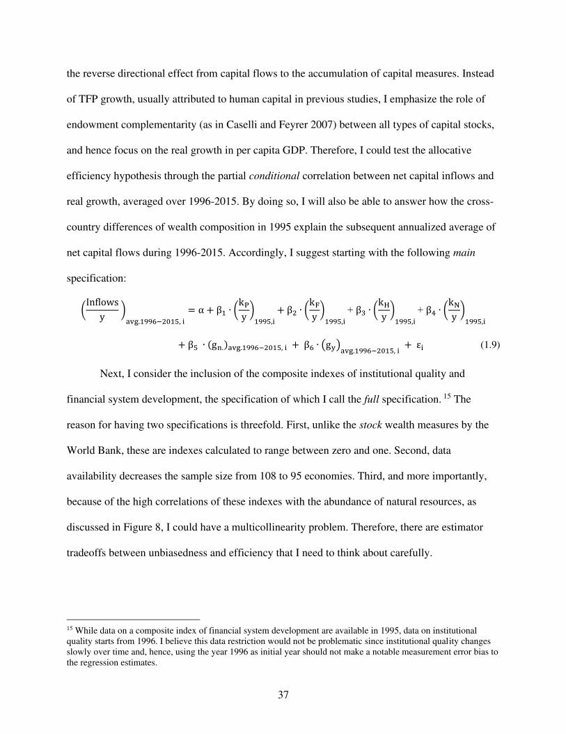
37

the reverse directional effect from capital flows to the accumulation of capital measures. Instead

of TFP growth, usually attributed to human capital in previous studies, I emphasize the role of

endowment complementarity (as in Caselli and Feyrer 2007) between all types of capital stocks,

and hence focus on the real growth in per capita GDP. Therefore, I could test the allocative

efficiency hypothesis through the partial conditional correlation between net capital inflows and

real growth, averaged over 1996-2015. By doing so, I will also be able to answer how the cross-

country differences of wealth composition in 1995 explain the subsequent annualized average of

net capital flows during 1996-2015. Accordingly, I suggest starting with the following main

specification:

(Inflowsy )avg.1996−2015, i = α + β1 ∙ (kPy )1995,i + β2 ∙ (kFy )1995,i + β3 ∙ (kHy )1995,i + β4 ∙ (kNy )1995,i + β5 ∙ (gn.)avg.1996−2015, i + β6 ∙ (gy)avg.1996−2015, i + εi (1.9)

Next, I consider the inclusion of the composite indexes of institutional quality and

financial system development, the specification of which I call the full specification. 15 The

reason for having two specifications is threefold. First, unlike the stock wealth measures by the

World Bank, these are indexes calculated to range between zero and one. Second, data

availability decreases the sample size from 108 to 95 economies. Third, and more importantly,

because of the high correlations of these indexes with the abundance of natural resources, as

discussed in Figure 8, I could have a multicollinearity problem. Therefore, there are estimator

tradeoffs between unbiasedness and efficiency that I need to think about carefully.

15 While data on a composite index of financial system development are available in 1995, data on institutional quality starts from 1996. I believe this data restriction would not be problematic since institutional quality changes slowly over time and, hence, using the year 1996 as initial year should not make a notable measurement error bias to the regression estimates.

38

It should be noted that I run equation (1.9) three times because of the three measures of

net capital inflows, as discussed in section 1.2.2. This way allows us to disentangle

commonalities and differences across the measures. All regressions are run with White

heteroscedasticity-consistent standard errors that address the possible heteroskedasticity due to

economy-size differences.

1.5.3 Robustness Checks

After conducting the main regression analysis, I will run a battery of robustness checks.

First, the period of study during 1995-2015 is characterized by many volatile episodes of capital

flows which might have caused a structural change in the relationship. Such episodes include the

1997 Asian financial crisis, the 2001 dot-com bubble, 2008-9 Global Financial Crisis (GFC),

followed by the European sovereign debt crisis and finally the 2013 FED taper-tantrum. All of

which are believed to impact certain types of capital flows, except for the GFC that could have a

possible structural change to the net (total) capital inflows. Therefore, I test for a structural

change due to the 2008-09 GFC, using a dummy-variable technique. Second, the allocation

puzzle argument by Gourinchas and Jeanne (2013) is, in fact, on a sample of EMDEs, so I

exclude OECD countries. Third, due to the relative importance and characteristics of China and

India, I also drop them too. Fourth, I exclude potential influential observations, identified by

informal and formal statistical tests. In addition, instead of the ordinary least square regression, I

run robust and quantile regression analyses. The robust regression analysis uses iteratively

reweighted least-squares based on Cook’s Distance method in which lower weights are assigned

to observations with values greater than one. The quantile regression is based on minimizing the

least absolute deviations from the median.16 Next, I run an OLS regression with fixed effects for

16 The quantile regression is also known as a Least Absolute Deviations (LAD) regression.

39

income and regional groups to control for unobserved heterogeneity. Finally, due to our concern

about the measure of human capital wealth, I use average years of schooling as in Barro and Lee

(2013).

Results

This section starts off by reporting the regression estimates of the main specification

sample, which consists of 108 countries.17 Then, I report the regression estimates with regard to

the robustness checks.

1.6.1 Regression Estimates

The main contribution of the current study is to highlight the role of natural resource

abundance, particularly its decomposition into the subsoil and non-soil types, in explaining the

variations in the subsequent average of net capital inflows. Table 1.5 reports the main

specification estimates using the three measures of net capital inflows.18 First, the initial

abundance of subsoil resource abundance enters with a significantly negative coefficient,

whereas non-subsoil resource abundance associates with a positive coefficient (as in columns 1

and 3). Interestingly, the measure ΔNFL (as in column 2) show that there is an important role of

the valuation effects, as these two coefficients turn to become no longer statistically significant.

This could be interpreted that the valuation effects mute the impact. Moreover, while the

measures in columns 1 and 3 show there is evidence on the negative association between the

initial abundance of net foreign assets and subsequent net total capital inflows, column 2 shows

the reverse in the sign which is significant because of the role of valuation effects. This implies

that only by ignoring the valuations effects, I find supporting evidence on the role of natural

17 Liberia is the only country that I have excluded. It seems an obvious influential observation as could be identified by both informal and formal statistical checks. 18 Table 1.5 considers the decomposition of natural capital into two types. By contrast, using the aggregate natural resource abundance produces meaningless estimates as shown in the appendix Table A5.

40

resources and the persistence of global imbalance. Thus, countries with CA surpluses in the past

(reflected in higher NFA positions) have continued to be associated with subsequent net capital

outflows (or CA surpluses). Besides, estimates of the three measures show no evidence on the

neoclassical efficient allocation hypothesis, captured by the insignificant coefficient on the real

per capita growth.

In addition, there is weak evidence on human capital abundance but with a negative sign,

only with the second measure regression (column 2 of Table 1.5). Nevertheless, that raises

concerns over the use of this measure of human capital in a cross-country context. That is, it is

based on households’ discounted life-time expected earnings, which I argue that it captures labor

cheapness rather than skills in a cross-country context. Accordingly, I could interpret the

negative coefficient as follow: all else being equal, semi-industrialized countries with lower

expected lifetime earnings are associated with a subsequent annual average of net capital

outflows over average.19

Besides the statistical significance, I should identify the economic significance which

matters for policymaking. The estimates in column (1) suggest that an increase by one standard

deviation (1.14) in the initial abundance of subsoil resources, ceteris paribus, associates with a

reduction in the ratio of subsequent annual average net capital inflows to GDP by 3.61

percentage points over the next two decades. Put differently, all else being equal, an increase in

the initial abundance of subsoil resources from the 25th percentile to 75th percentile associates

with a reduction in the ratio of subsequent annual average net capital inflows to GDP by about

19 I validate the normality of residuals using a kernel density plot. I also find that there is no indication of multicollinearity in this main specification as suggested by the values of variance inflation factors (VIF) and condition indices (CI). Following the role of thumps discussed by Gujarati and Porter (2009, pp. 337-342), I find that no value of VIFs and CIs exceed 5 and 20, respectively. Therefore, there should be no concern about multicollinearity in the main specification. All of which suggest that we could draw inferences from the estimates.

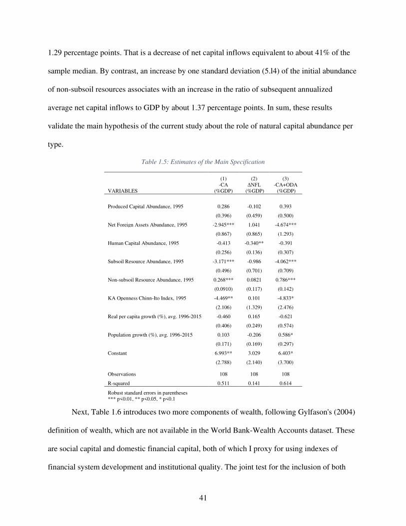
41

1.29 percentage points. That is a decrease of net capital inflows equivalent to about 41% of the

sample median. By contrast, an increase by one standard deviation (5.l4) of the initial abundance

of non-subsoil resources associates with an increase in the ratio of subsequent annualized

average net capital inflows to GDP by about 1.37 percentage points. In sum, these results

validate the main hypothesis of the current study about the role of natural capital abundance per

type.

Table 1.5: Estimates of the Main Specification

(1) (2) (3)

VARIABLES -CA

(%GDP) ΔNFL

(%GDP) -CA+ODA (%GDP)

Produced Capital Abundance, 1995 0.286 -0.102 0.393

(0.396) (0.459) (0.500)

Net Foreign Assets Abundance, 1995 -2.945*** 1.041 -4.674***

(0.867) (0.865) (1.293)

Human Capital Abundance, 1995 -0.413 -0.340** -0.391

(0.256) (0.136) (0.307)

Subsoil Resource Abundance, 1995 -3.171*** -0.986 -4.062***

(0.496) (0.701) (0.709)

Non-subsoil Resource Abundance, 1995 0.268*** 0.0821 0.786***

(0.0910) (0.117) (0.142)

KA Openness Chinn-Ito Index, 1995 -4.469** 0.101 -4.833*

(2.106) (1.329) (2.476)

Real per capita growth (%), avg. 1996-2015 -0.460 0.165 -0.621

(0.406) (0.249) (0.574)

Population growth (%), avg. 1996-2015 0.103 -0.206 0.586*

(0.171) (0.169) (0.297)

Constant 6.993** 3.029 6.403*

(2.788) (2.140) (3.700)

Observations 108 108 108

R-squared 0.511 0.141 0.614

Robust standard errors in parentheses *** p<0.01, ** p<0.05, * p<0.1

Next, Table 1.6 introduces two more components of wealth, following Gylfason's (2004)

definition of wealth, which are not available in the World Bank-Wealth Accounts dataset. These

are social capital and domestic financial capital, both of which I proxy for using indexes of

financial system development and institutional quality. The joint test for the inclusion of both

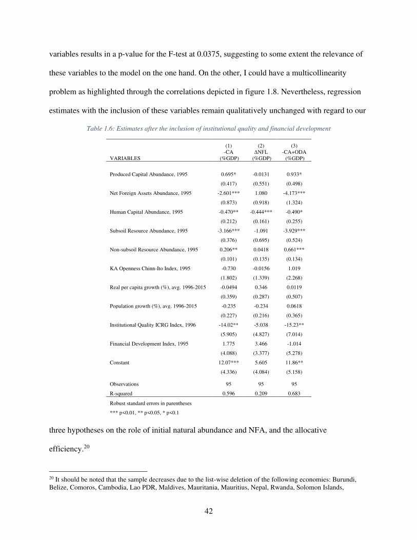
42

variables results in a p-value for the F-test at 0.0375, suggesting to some extent the relevance of

these variables to the model on the one hand. On the other, I could have a multicollinearity

problem as highlighted through the correlations depicted in figure 1.8. Nevertheless, regression

estimates with the inclusion of these variables remain qualitatively unchanged with regard to our

Table 1.6: Estimates after the inclusion of institutional quality and financial development

(1) (2) (3)

VARIABLES -CA

(%GDP) ΔNFL


Produced Capital Abundance, 1995 0.695* -0.0131 0.933*

(0.417) (0.551) (0.498)


(0.873) (0.918) (1.324)

Human Capital Abundance, 1995 -0.470** -0.444*** -0.490*

(0.212) (0.161) (0.255)


(0.376) (0.695) (0.524)

Non-subsoil Resource Abundance, 1995 0.206** 0.0418 0.661***

(0.101) (0.135) (0.134)

KA Openness Chinn-Ito Index, 1995 -0.730 -0.0156 1.019

(1.802) (1.339) (2.268)

Real per capita growth (%), avg. 1996-2015 -0.0494 0.346 0.0119

(0.359) (0.287) (0.507)

Population growth (%), avg. 1996-2015 -0.235 -0.234 0.0618

(0.227) (0.216) (0.365)

Institutional Quality ICRG Index, 1996 -14.02** -5.038 -15.23**

(5.905) (4.827) (7.014)

Financial Development Index, 1995 1.775 3.466 -1.014

(4.088) (3.377) (5.278)

Constant 12.07*** 5.605 11.86**

(4.336) (4.084) (5.158)


R-squared 0.596 0.209 0.683

Robust standard errors in parentheses

*** p<0.01, ** p<0.05, * p<0.1

three hypotheses on the role of initial natural abundance and NFA, and the allocative

efficiency.20

20 It should be noted that the sample decreases due to the list-wise deletion of the following economies: Burundi, Belize, Comoros, Cambodia, Lao PDR, Maldives, Mauritania, Mauritius, Nepal, Rwanda, Solomon Islands,

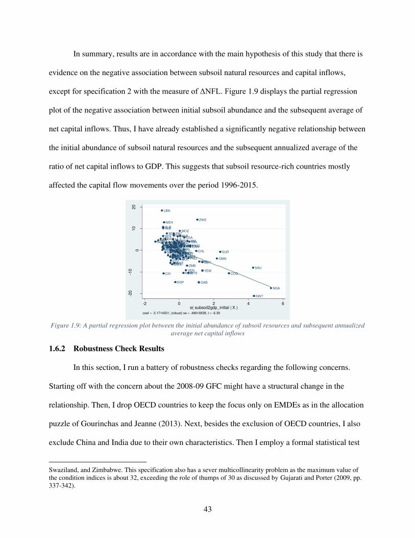
43

In summary, results are in accordance with the main hypothesis of this study that there is

evidence on the negative association between subsoil natural resources and capital inflows,

except for specification 2 with the measure of ΔNFL. Figure 1.9 displays the partial regression

plot of the negative association between initial subsoil abundance and the subsequent average of

net capital inflows. Thus, I have already established a significantly negative relationship between

the initial abundance of subsoil natural resources and the subsequent annualized average of the

ratio of net capital inflows to GDP. This suggests that subsoil resource-rich countries mostly

affected the capital flow movements over the period 1996-2015.

Figure 1.9: A partial regression plot between the initial abundance of subsoil resources and subsequent annualized

average net capital inflows

1.6.2 Robustness Check Results

In this section, I run a battery of robustness checks regarding the following concerns.

Starting off with the concern about the 2008-09 GFC might have a structural change in the

relationship. Then, I drop OECD countries to keep the focus only on EMDEs as in the allocation

puzzle of Gourinchas and Jeanne (2013). Next, besides the exclusion of OECD countries, I also

exclude China and India due to their own characteristics. Then I employ a formal statistical test

Swaziland, and Zimbabwe. This specification also has a sever multicollinearity problem as the maximum value of the condition indices is about 32, exceeding the role of thumps of 30 as discussed by Gujarati and Porter (2009, pp. 337-342).

COMNERBLZ

LBN

KENMLISEN

TUR

SLB

BFA

SLE

MDG

CIV

JOR

MDV

BHR

GRC

GMBUGAGTM

BDI

RWAITASLV

PAK

HND

MWI

BGD

THA

ARG

GHA

NPL

MAR

PRY

BGRSWZBELHUN

BWA

ETH

AUT

DNKFIN

MLT

DEU

PER

NIC

FRA

PRT

TZA

SWE

CRIESPTGO

NAM

SGP

PHL

TUN

KHM

URYLKAMUS

NLD

JPN

GBR

BRACOL

PAN

MEXLAO

AUS

MOZ

CMR

ALB

BOL

DOM

IND

POLZAF

ECUEGY

NOR

KOR

IRL

USA

MRT

IDN

VEN

VNM

ZMB

JAM

PNG

MYS

GIN

CANMNG

CHL

ZWE

GAB

CHNGUY

YEM

OMN

SUR

COG

SAU

KWT

NGA

-20

-10

01

02

0

-2 0 2 4 6e( subsoil2gdp_initial | X )

coef = -3.1714501, (robust) se = .49616938, t = -6.39

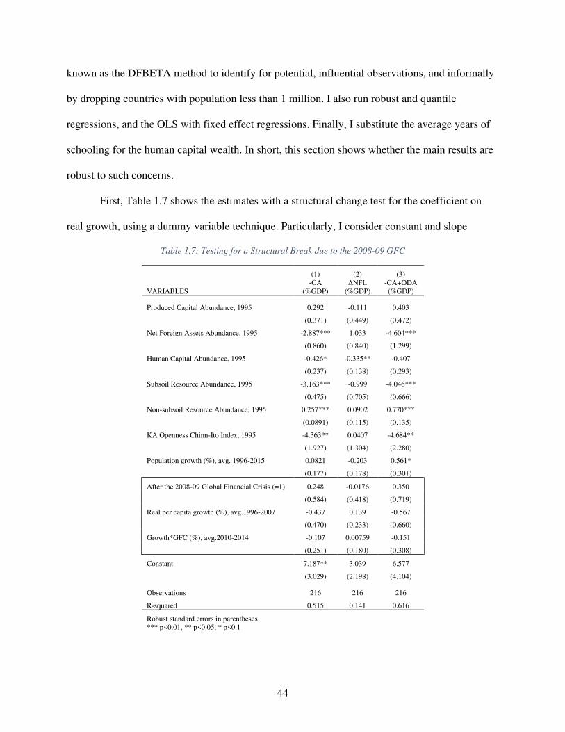
44

known as the DFBETA method to identify for potential, influential observations, and informally

by dropping countries with population less than 1 million. I also run robust and quantile

regressions, and the OLS with fixed effect regressions. Finally, I substitute the average years of

schooling for the human capital wealth. In short, this section shows whether the main results are

robust to such concerns.

First, Table 1.7 shows the estimates with a structural change test for the coefficient on

real growth, using a dummy variable technique. Particularly, I consider constant and slope

Table 1.7: Testing for a Structural Break due to the 2008-09 GFC

(1) (2) (3)

VARIABLES -CA

(%GDP) ΔNFL



(0.371) (0.449) (0.472)


(0.860) (0.840) (1.299)

Human Capital Abundance, 1995 -0.426* -0.335** -0.407

(0.237) (0.138) (0.293)


(0.475) (0.705) (0.666)


(0.0891) (0.115) (0.135)

KA Openness Chinn-Ito Index, 1995 -4.363** 0.0407 -4.684**

(1.927) (1.304) (2.280)


(0.177) (0.178) (0.301)

After the 2008-09 Global Financial Crisis (=1) 0.248 -0.0176 0.350

(0.584) (0.418) (0.719)

Real per capita growth (%), avg.1996-2007 -0.437 0.139 -0.567

(0.470) (0.233) (0.660)

Growth*GFC (%), avg.2010-2014 -0.107 0.00759 -0.151

(0.251) (0.180) (0.308)

Constant 7.187** 3.039 6.577

(3.029) (2.198) (4.104)


R-squared 0.515 0.141 0.616


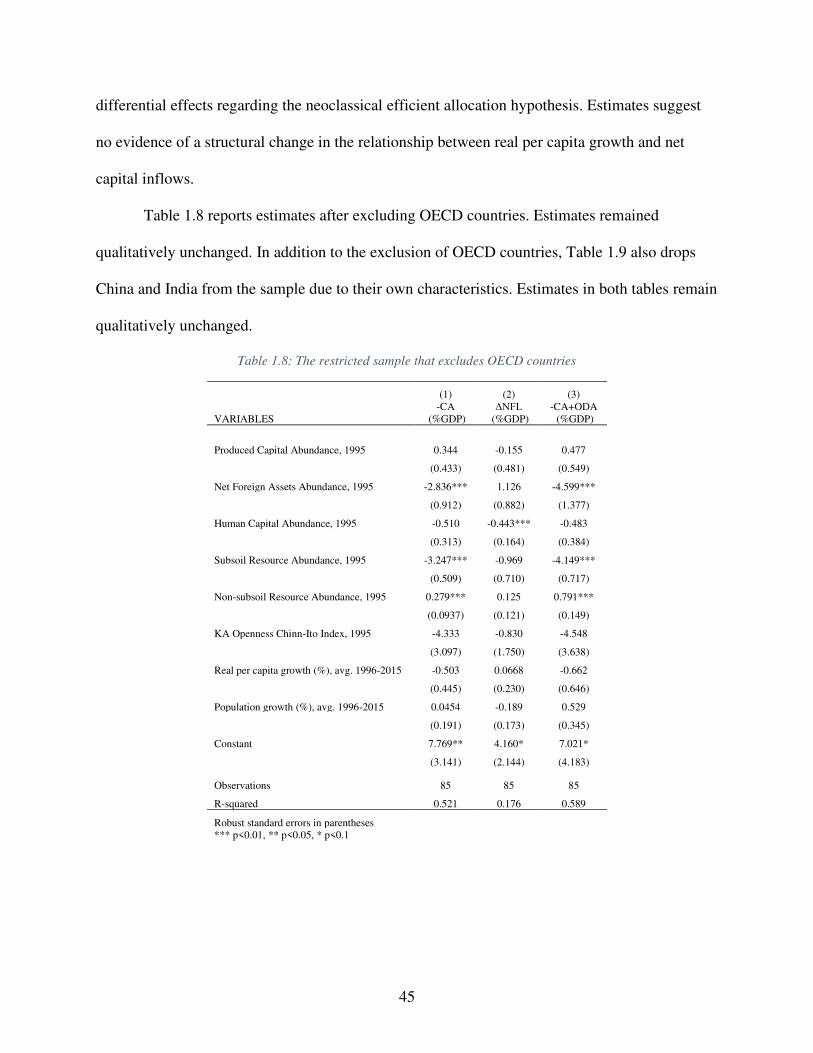
45

differential effects regarding the neoclassical efficient allocation hypothesis. Estimates suggest

no evidence of a structural change in the relationship between real per capita growth and net

capital inflows.

Table 1.8 reports estimates after excluding OECD countries. Estimates remained

qualitatively unchanged. In addition to the exclusion of OECD countries, Table 1.9 also drops

China and India from the sample due to their own characteristics. Estimates in both tables remain

qualitatively unchanged.

Table 1.8: The restricted sample that excludes OECD countries

(1) (2) (3)

VARIABLES -CA

(%GDP) ΔNFL



(0.433) (0.481) (0.549)


(0.912) (0.882) (1.377)

Human Capital Abundance, 1995 -0.510 -0.443*** -0.483

(0.313) (0.164) (0.384)


(0.509) (0.710) (0.717)


(0.0937) (0.121) (0.149)

KA Openness Chinn-Ito Index, 1995 -4.333 -0.830 -4.548

(3.097) (1.750) (3.638)


(0.445) (0.230) (0.646)

Population growth (%), avg. 1996-2015 0.0454 -0.189 0.529

(0.191) (0.173) (0.345)

Constant 7.769** 4.160* 7.021*

(3.141) (2.144) (4.183)


R-squared 0.521 0.176 0.589


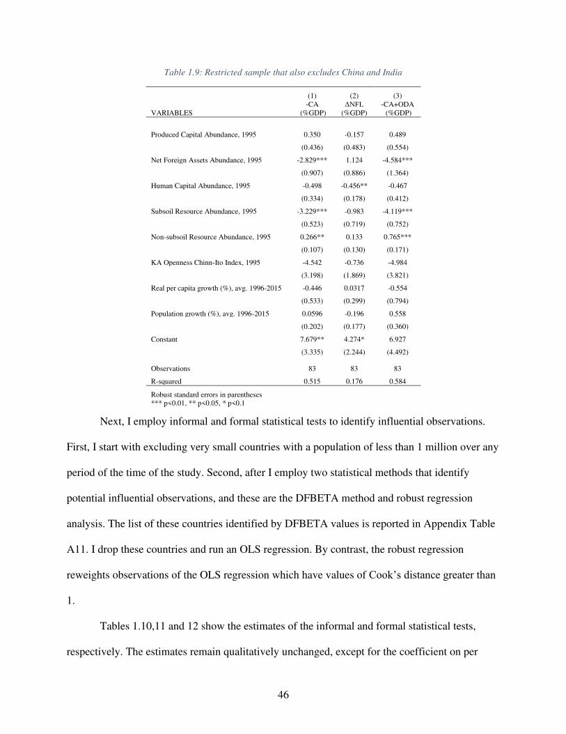
46

Table 1.9: Restricted sample that also excludes China and India

(1) (2) (3)

VARIABLES -CA

(%GDP) ΔNFL



(0.436) (0.483) (0.554)


(0.907) (0.886) (1.364)


(0.334) (0.178) (0.412)


(0.523) (0.719) (0.752)


(0.107) (0.130) (0.171)


(3.198) (1.869) (3.821)


(0.533) (0.299) (0.794)


(0.202) (0.177) (0.360)

Constant 7.679** 4.274* 6.927

(3.335) (2.244) (4.492)


R-squared 0.515 0.176 0.584


Next, I employ informal and formal statistical tests to identify influential observations.

First, I start with excluding very small countries with a population of less than 1 million over any

period of the time of the study. Second, after I employ two statistical methods that identify

potential influential observations, and these are the DFBETA method and robust regression

analysis. The list of these countries identified by DFBETA values is reported in Appendix Table

A11. I drop these countries and run an OLS regression. By contrast, the robust regression

reweights observations of the OLS regression which have values of Cook’s distance greater than

1.

Tables 1.10,11 and 12 show the estimates of the informal and formal statistical tests,

respectively. The estimates remain qualitatively unchanged, except for the coefficient on per

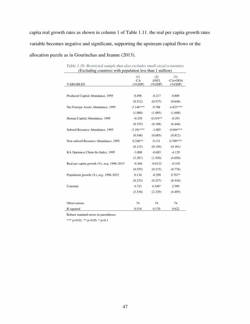
47

capita real growth rates as shown in column 1 of Table 1.11. the real per capita growth rates

variable becomes negative and significant, supporting the upstream capital flows or the

allocation puzzle as in Gourinchas and Jeanne (2013).

Table 1.10: Restricted sample that also excludes small-sized economies

(Excluding countries with population less than 1 million)

(1) (2) (3)

VARIABLES -CA

(%GDP) ΔNFL



(0.512) (0.537) (0.648)


(1.080) (1.085) (1.608)


(0.355) (0.188) (0.446)


(0.548) (0.685) (0.812)


(0.115) (0.156) (0.181)


(3.287) (1.930) (4.050)

Real per capita growth (%), avg. 1996-2015 -0.364 -0.0122 -0.310

(0.555) (0.315) (0.776)


(0.233) (0.257) (0.410)

Constant 4.723 4.340* 2.589

(3.536) (2.329) (4.495)


R-squared 0.534 0.170 0.622


*** p<0.01, ** p<0.05, * p<0.1

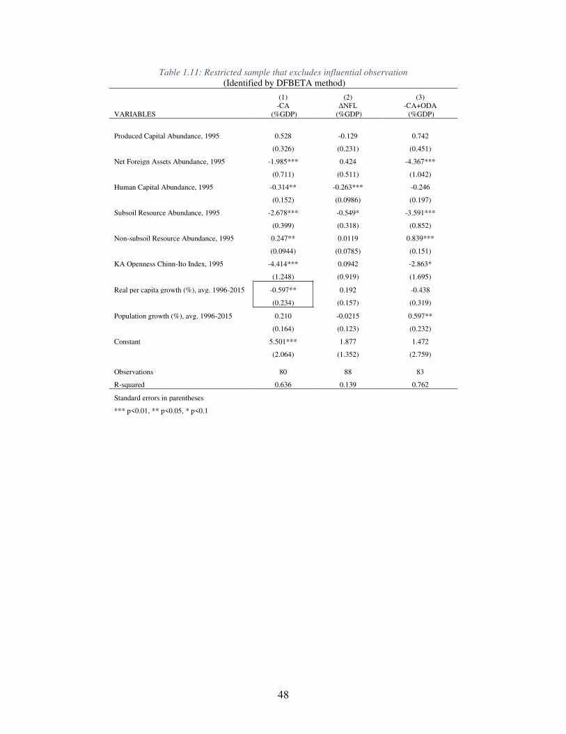
48

Table 1.11: Restricted sample that excludes influential observation

(Identified by DFBETA method)

(1) (2) (3)

VARIABLES -CA

(%GDP) ΔNFL



(0.326) (0.231) (0.451)


(0.711) (0.511) (1.042)

Human Capital Abundance, 1995 -0.314** -0.263*** -0.246

(0.152) (0.0986) (0.197)

Subsoil Resource Abundance, 1995 -2.678*** -0.549* -3.591***

(0.399) (0.318) (0.852)


(0.0944) (0.0785) (0.151)

KA Openness Chinn-Ito Index, 1995 -4.414*** 0.0942 -2.863*

(1.248) (0.919) (1.695)

Real per capita growth (%), avg. 1996-2015 -0.597** 0.192 -0.438

(0.234) (0.157) (0.319)

Population growth (%), avg. 1996-2015 0.210 -0.0215 0.597**

(0.164) (0.123) (0.232)

Constant 5.501*** 1.877 1.472

(2.064) (1.352) (2.759)


R-squared 0.636 0.139 0.762

Standard errors in parentheses

*** p<0.01, ** p<0.05, * p<0.1

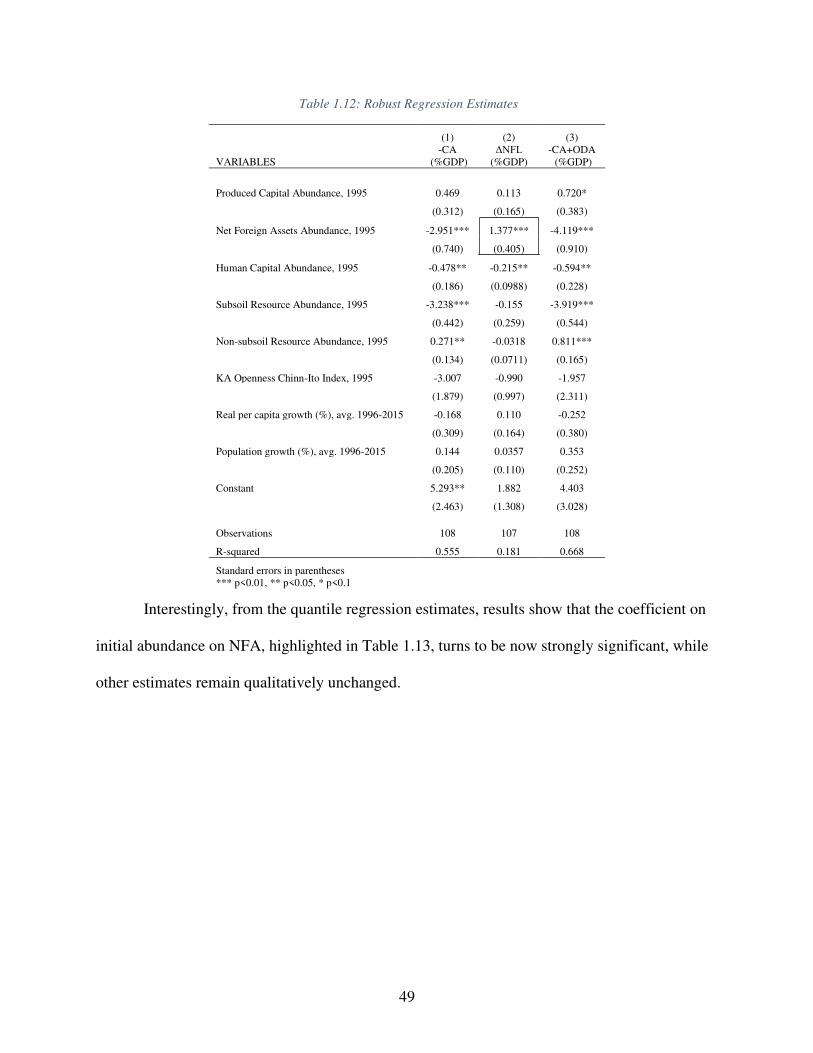
49

Table 1.12: Robust Regression Estimates

(1) (2) (3)

VARIABLES -CA

(%GDP) ΔNFL


Produced Capital Abundance, 1995 0.469 0.113 0.720*

(0.312) (0.165) (0.383)

Net Foreign Assets Abundance, 1995 -2.951*** 1.377*** -4.119***

(0.740) (0.405) (0.910)

Human Capital Abundance, 1995 -0.478** -0.215** -0.594**

(0.186) (0.0988) (0.228)


(0.442) (0.259) (0.544)

Non-subsoil Resource Abundance, 1995 0.271** -0.0318 0.811***

(0.134) (0.0711) (0.165)


(1.879) (0.997) (2.311)


(0.309) (0.164) (0.380)

Population growth (%), avg. 1996-2015 0.144 0.0357 0.353

(0.205) (0.110) (0.252)

Constant 5.293** 1.882 4.403

(2.463) (1.308) (3.028)


R-squared 0.555 0.181 0.668

Standard errors in parentheses *** p<0.01, ** p<0.05, * p<0.1

Interestingly, from the quantile regression estimates, results show that the coefficient on

initial abundance on NFA, highlighted in Table 1.13, turns to be now strongly significant, while

other estimates remain qualitatively unchanged.

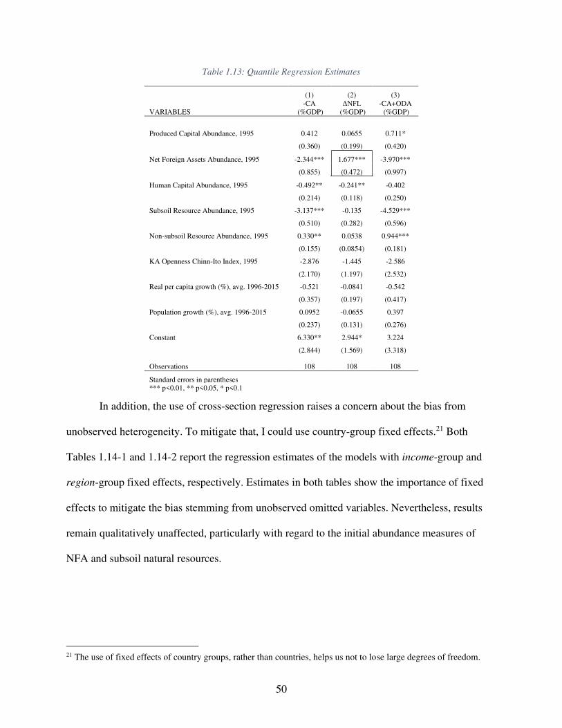
50

Table 1.13: Quantile Regression Estimates

(1) (2) (3)

VARIABLES -CA

(%GDP) ΔNFL



(0.360) (0.199) (0.420)

Net Foreign Assets Abundance, 1995 -2.344*** 1.677*** -3.970***

(0.855) (0.472) (0.997)

Human Capital Abundance, 1995 -0.492** -0.241** -0.402

(0.214) (0.118) (0.250)


(0.510) (0.282) (0.596)


(0.155) (0.0854) (0.181)


(2.170) (1.197) (2.532)


(0.357) (0.197) (0.417)


(0.237) (0.131) (0.276)

Constant 6.330** 2.944* 3.224

(2.844) (1.569) (3.318)


Standard errors in parentheses *** p<0.01, ** p<0.05, * p<0.1

In addition, the use of cross-section regression raises a concern about the bias from

unobserved heterogeneity. To mitigate that, I could use country-group fixed effects.21 Both

Tables 1.14-1 and 1.14-2 report the regression estimates of the models with income-group and

region-group fixed effects, respectively. Estimates in both tables show the importance of fixed

effects to mitigate the bias stemming from unobserved omitted variables. Nevertheless, results

remain qualitatively unaffected, particularly with regard to the initial abundance measures of

NFA and subsoil natural resources.

21 The use of fixed effects of country groups, rather than countries, helps us not to lose large degrees of freedom.

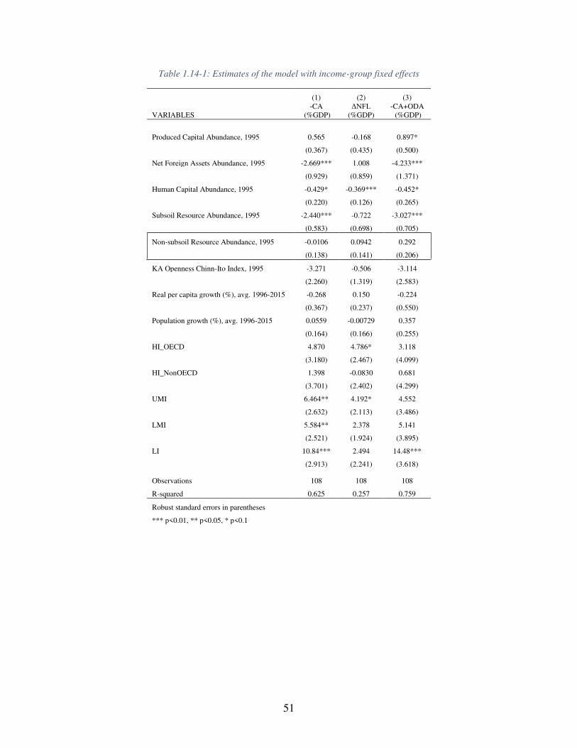
51

Table 1.14-1: Estimates of the model with income-group fixed effects

(1) (2) (3)

VARIABLES -CA

(%GDP) ΔNFL


Produced Capital Abundance, 1995 0.565 -0.168 0.897*

(0.367) (0.435) (0.500)


(0.929) (0.859) (1.371)

Human Capital Abundance, 1995 -0.429* -0.369*** -0.452*

(0.220) (0.126) (0.265)


(0.583) (0.698) (0.705)

Non-subsoil Resource Abundance, 1995 -0.0106 0.0942 0.292

(0.138) (0.141) (0.206)


(2.260) (1.319) (2.583)


(0.367) (0.237) (0.550)


(0.164) (0.166) (0.255)

HI_OECD 4.870 4.786* 3.118

(3.180) (2.467) (4.099)

HI_NonOECD 1.398 -0.0830 0.681

(3.701) (2.402) (4.299)

UMI 6.464** 4.192* 4.552

(2.632) (2.113) (3.486)

LMI 5.584** 2.378 5.141

(2.521) (1.924) (3.895)

LI 10.84*** 2.494 14.48***

(2.913) (2.241) (3.618)


R-squared 0.625 0.257 0.759


*** p<0.01, ** p<0.05, * p<0.1

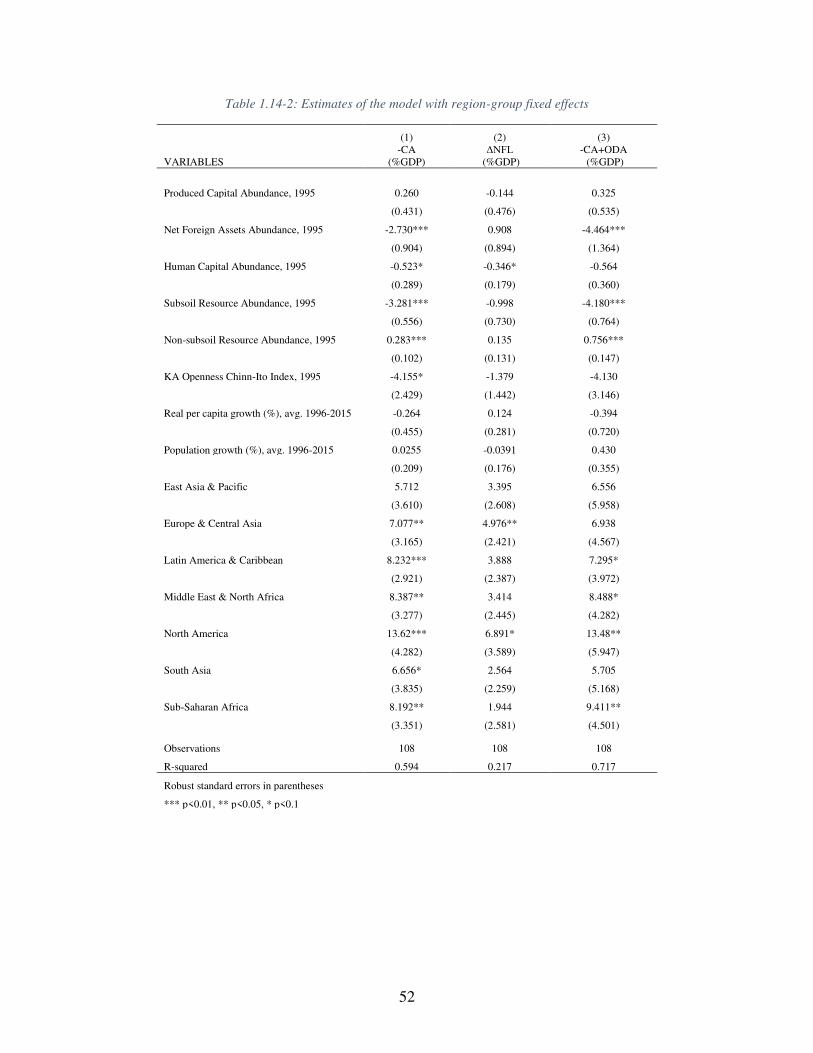
52

Table 1.14-2: Estimates of the model with region-group fixed effects

(1) (2) (3)

VARIABLES -CA

(%GDP) ΔNFL



(0.431) (0.476) (0.535)


(0.904) (0.894) (1.364)

Human Capital Abundance, 1995 -0.523* -0.346* -0.564

(0.289) (0.179) (0.360)


(0.556) (0.730) (0.764)


(0.102) (0.131) (0.147)

KA Openness Chinn-Ito Index, 1995 -4.155* -1.379 -4.130

(2.429) (1.442) (3.146)


(0.455) (0.281) (0.720)


(0.209) (0.176) (0.355)

East Asia & Pacific 5.712 3.395 6.556

(3.610) (2.608) (5.958)

Europe & Central Asia 7.077** 4.976** 6.938

(3.165) (2.421) (4.567)

Latin America & Caribbean 8.232*** 3.888 7.295*

(2.921) (2.387) (3.972)

Middle East & North Africa 8.387** 3.414 8.488*

(3.277) (2.445) (4.282)

North America 13.62*** 6.891* 13.48**

(4.282) (3.589) (5.947)

South Asia 6.656* 2.564 5.705

(3.835) (2.259) (5.168)

Sub-Saharan Africa 8.192** 1.944 9.411**

(3.351) (2.581) (4.501)


R-squared 0.594 0.217 0.717


*** p<0.01, ** p<0.05, * p<0.1

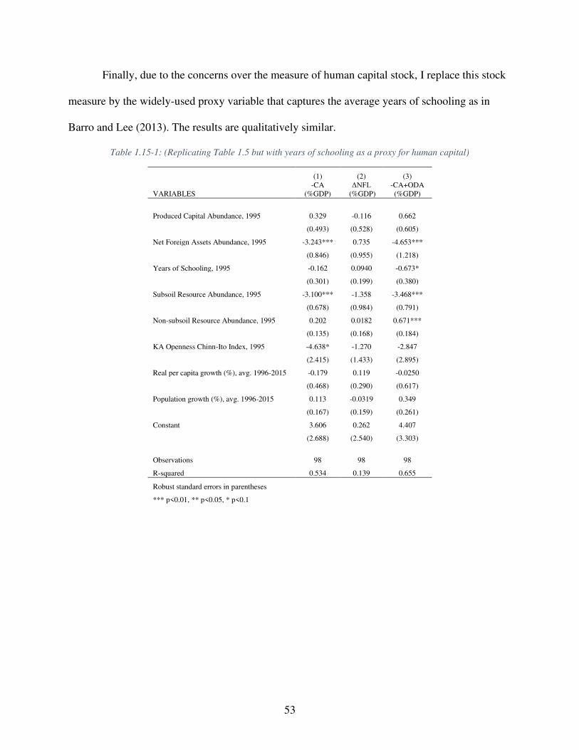
53

Finally, due to the concerns over the measure of human capital stock, I replace this stock

measure by the widely-used proxy variable that captures the average years of schooling as in

Barro and Lee (2013). The results are qualitatively similar.

Table 1.15-1: (Replicating Table 1.5 but with years of schooling as a proxy for human capital)

(1) (2) (3)

VARIABLES -CA

(%GDP) ΔNFL



(0.493) (0.528) (0.605)


(0.846) (0.955) (1.218)

Years of Schooling, 1995 -0.162 0.0940 -0.673*

(0.301) (0.199) (0.380)


(0.678) (0.984) (0.791)

Non-subsoil Resource Abundance, 1995 0.202 0.0182 0.671***

(0.135) (0.168) (0.184)

KA Openness Chinn-Ito Index, 1995 -4.638* -1.270 -2.847

(2.415) (1.433) (2.895)


(0.468) (0.290) (0.617)


(0.167) (0.159) (0.261)

Constant 3.606 0.262 4.407

(2.688) (2.540) (3.303)


R-squared 0.534 0.139 0.655


*** p<0.01, ** p<0.05, * p<0.1

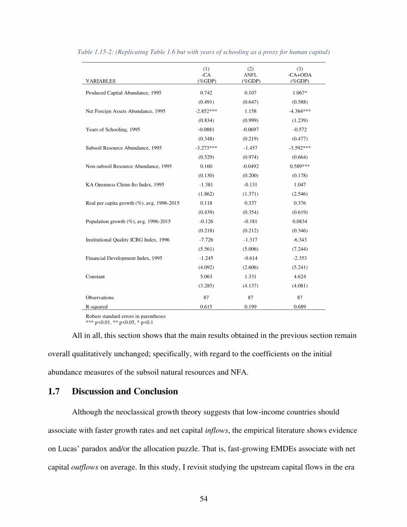
54

Table 1.15-2: (Replicating Table 1.6 but with years of schooling as a proxy for human capital)

(1) (2) (3)

VARIABLES -CA

(%GDP) ΔNFL



(0.491) (0.647) (0.588)


(0.834) (0.999) (1.239)

Years of Schooling, 1995 -0.0881 -0.0697 -0.572

(0.348) (0.219) (0.477)


(0.529) (0.974) (0.664)

Non-subsoil Resource Abundance, 1995 0.160 -0.0492 0.589***

(0.130) (0.200) (0.178)


(1.862) (1.371) (2.546)

Real per capita growth (%), avg. 1996-2015 0.118 0.337 0.376

(0.439) (0.354) (0.619)


(0.218) (0.212) (0.346)

Institutional Quality ICRG Index, 1996 -7.726 -1.317 -6.343

(5.561) (5.006) (7.244)

Financial Development Index, 1995 -1.245 -0.614 -2.353

(4.092) (2.606) (5.241)

Constant 5.063 1.331 4.624

(3.285) (4.137) (4.081)


R-squared 0.615 0.199 0.689


All in all, this section shows that the main results obtained in the previous section remain

overall qualitatively unchanged; specifically, with regard to the coefficients on the initial

abundance measures of the subsoil natural resources and NFA.

Discussion and Conclusion

Although the neoclassical growth theory suggests that low-income countries should

associate with faster growth rates and net capital inflows, the empirical literature shows evidence

on Lucas’ paradox and/or the allocation puzzle. That is, fast-growing EMDEs associate with net

capital outflows on average. In this study, I revisit studying the upstream capital flows in the era

55

of financial globalization during 1995-2015 while emphasizing the role of natural resource

abundance. I take advantage of a recently released data on wealth accounts by the World Bank,

supplemented by data on other relevant variables. Wealth is defined as the sum of produced

capital, human capital, natural capital, NFA (Lange, Wodon, and Carey 2018), plus social capital

and domestic financial capital (Gylfason 2004). Moreover, I use three alternative measures of net

total capital inflows, the typical one of which is the negative CA while the others incorporate

official aid flows and valuation effects, respectfully. Interestingly, the typical and aid-adjusted

CA measures produce similar estimates and, more importantly, with regard to natural capital. By

using these two measures, I find statistical evidence on the negative association between the

initial abundance of subsoil natural capital and net capital inflows. Besides, I find supporting

evidence on the persistence of global imbalances, captured by the negative coefficient on the

initial NFA abundance. On the contrary, there is no supporting evidence on the allocative

efficiency hypothesis— the association between productivity growth and net capital inflows.

This could stem from the large sample size rather than the productivity growth measure.

Previous studies such as Chinn and Prasad (2003) and Alfaro et al. (2014) find that as the sample

size increases, the relationship becomes either insignificant or weakly and positively significant.

Alfaro et al. also show that replacing the average real per capita growth with the catch-up

productivity measure of Gourinchas and Jeanne (2013) does not explain the relationship

differences.

Interestingly, the measure that incorporates valuation effects (ΔNFL) alter the previous

main results, implying great importance for the role of valuation effects by reversing the sign on

initial NFA abundance although being statistically insignificant. In this regard, Gourinchas and

Rey (2005) demonstrate that the US has enjoyed an exorbitant privilege in which the total return

56

on its foreign assets exceeds its foreign liabilities, despite being a debtor country, especially in

the post-Bretton Woods period till 2004. They conclude that valuation adjustment has played a

stabilization role for the US. In a later study, Gourinchas and Rey (2015) also demonstrate that

valuation effects have played an important role in the current international financial system in

which G7 countries were the largest winners while the BRICS countries were losers.

This study, therefore, shows that the introduction of natural capital allows for the role of

economic policy, unlike the standard neoclassical model. Policymakers in EMDEs can decide on

how to utilize the stocks of natural resources, so they impact the GDP level and growth (through

liquidation rather than productive investment). With capital mobility, as in the financial

globalization era we live in, policymakers have the potential to mitigate the Dutch disease effects

through ameliorating the appreciation pressure in the exchange rate. If the accumulation of NFA

is implemented as suggested by PIH, smoothing not only consumption but also investments in

physical and human capital, then KN could also crowd in KF in the development process. In sum,

the extended open-economy framework suggests that the PIH about smoothing both

consumption and investment in human capital and physical capital.

Particularly, this study shows statistical evidence that the accumulation in the form of

NFA positions by subsoil-rich economies explains a large part of the upstream capital flows

phenomenon. The assumption of imperfect capital mobility is critical to the seminal models of

uneven development (Krugman 1981), and the natural resource-curse (Rodriguez and Sachs

1999). Resource-rich countries can benefit from capital mobility to break the unsustainable

overconsumption argument by Rodriguez and Sachs (1999). Rodriguez and Sachs, acknowledge

the role of international capital markets in breaking out the unsustainable overconsumption. They

state:

57

If an economy can invest its resource windfalls in international assets that pay permanent

annuities, then the problem we are alluding to could not occur. Any economy

experiencing a resource boom will invest it and permanently consume the interest it earns

on that asset (p. 278).

Moreover, while Gourinchas and Jeanne (2013) attribute the allocation puzzle to the

capacity constraint on investment, rather than saving, I argue that the underlying cause could be

about the abundance of natural capital in EMDEs through the Dutch disease effects.22 That is, the

Dutch disease effects cause not only an appreciation of the exchange rates, but also an expansion

of the resource sector that crowds out investment opportunities on the modern sector which has a

larger capacity for new investment. Besides, EMDEs could use international capital markets to

maintain their real exchange rates manageable, through the accumulation of foreign reserves, in

order to protect their exports’ competitiveness and mitigate the Dutch disease effects. This could

also be somehow linked to the argument of “fear of floating” by Calvo and Reinhart (2002).

Foreign reserve accumulation allows such subsoil countries to stabilize their exchange rates.

An important implication of the findings suggests the greater role of economic policy in

explaining the patterns of capital flows, unlike in the standard neoclassical growth theory

adopted by the previous literature of capital flows. Results suggest that the upstream flows could

be driven by foreign asset accumulation by subsoil-type endowed countries. On the other hand,

Table 1.4 shows that the high-income, non-OECD countries associate with the highest subsoil

abundance and slowest growth relatively over the last few decades. Therefore, while subsoil

resource-rich countries should adopt a policy mix of reserve accumulation and industrial policy,

data suggest the need for assigning more weight on the latter that could generate sustainable

22 In this regard, Hausmann, Rodrik, and Velasco (2005) explain growth diagnostics, and emphasize that lower growth performance could be either from saving or investment binding constraints.

58

rapid growth. It should be highlighted that besides the challenges for industrialization, any policy

framework should emphasize creating employment opportunities that keep pace with the

growing population. Also, reserve accumulation allows for the use of exchange rates as a

developmental policy tool as in the export-led growth strategy implemented by fast-growing

emerging Asian countries. Shortly, studies demonstrate that an undervalued or appropriate level

of the exchange rate could be a key support for real growth and for creating employment

opportunities (see, e.g., Frenkel and Taylor 2006; Rodrik 2008)

It should be noted that this study does not control for some important aspects that could

also affect capital flows. These include global real and financial factors (except for the structural

break test of 2008-09 GFC), the dollar hegemony, and the financial deregulation and innovations

in the advanced economies in the recent few decades.

59

Chapter 2

International Capital Movements and Global Imbalances:

The Role of Complementarities and Tradeoffs in Capital

Stocks

Introduction

Cross-border capital flows have important implications on the national level and the

global economy. Stable flows of foreign capital could augment the domestic accumulation of

physical capital and hence spur economic growth, while volatile flows increase the risks and

trigger financial and economic crises. Therefore, the determinants of capital flows have been

extensively investigated in the literature. The determinants could be broadly classified into two

groups: push (or external) factors and pull (or internal) factors. While the former includes a set of

variables that capture global economic and financial conditions, the latter focuses on country-

specific conditions (see, e.g., Hannan 2017; Koepke 2015).

In a previous study, I concentrated on the pull factors, as in the context of an extended

open-economy growth framework with a broad definition of wealth, so that the income level is a

function of total wealth.23 Following Gylfason (2004), total wealth (W) is defined as the sum of

the following components: produced capital and urban land (KP), net foreign asset position (KF),

natural capital (KN), human capital (KH), social capital, and domestic financial capital. While the

first four components are available in stock units in the data, the last two are proxied by

23 There is a minimum requirement of sustainable development based on a weak sustainability assumption (see Barbier 2007). Succinctly, proponents of the weak sustainability argue that natural capital and other types of capital could be somehow substitutes during the economic development process. Put simply, the minimum requirement of sustainable development is to maintain a non-decreasing per capita total wealth over time.

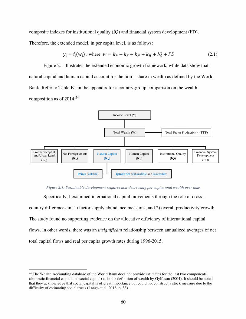
60

composite indexes for institutional quality (IQ) and financial system development (FD).

Therefore, the extended model, in per capita level, is as follows: yi = fi(wi) , where 𝑤 = 𝑘𝑃 + 𝑘𝐹 + 𝑘𝑁 + 𝑘𝐻 + 𝐼𝑄 + 𝐹𝐷 (2.1)

Figure 2.1 illustrates the extended economic growth framework, while data show that

natural capital and human capital account for the lion’s share in wealth as defined by the World

Bank. Refer to Table B1 in the appendix for a country-group comparison on the wealth

composition as of 2014.24

Figure 2.1: Sustainable development requires non-decreasing per capita total wealth over time

Specifically, I examined international capital movements through the role of cross-

country differences in: 1) factor supply abundance measures, and 2) overall productivity growth.

The study found no supporting evidence on the allocative efficiency of international capital

flows. In other words, there was an insignificant relationship between annualized averages of net

total capital flows and real per capita growth rates during 1996-2015.

24 The Wealth Accounting database of the World Bank does not provide estimates for the last two components (domestic financial capital and social capital) as in the definition of wealth by Gylfason (2004). It should be noted that they acknowledge that social capital is of great importance but could not construct a stock measure due to the difficulty of estimating social trusts (Lange et al. 2018, p. 33).

Income Level (Y)

Produced captial and Urban Land

(Kp)

Net Foreign Assets

(KF)

Natural Capital

(KN)

Prices (volatile) Quantities (exhaustible and renewable)

Human Capital

(KH)

Institutional Quality

(IQ)

Financial System Development

(FD)

Total Factor Productivity (TFP)Total Wealth (W)

61

The lack of evidence on the allocative efficiency of capital flows could be attributed to

the focus of that study on overall productivity growth. However, I could infer from the wide

literature that there could be specific, rather than overall, complementarity effects. First, the

productivity level of a country is understood as the technology measure of how efficiently or

effectively an economy combines all measures of factor supply in the production process, so our

focus on per capita real growth mostly captures the overall complementarity. The overall

complementarity is known as total factor productivity (TFP) or multi-factor productivity as in

Acemoglu (2009, p. 78). However, cross-border capital flows could target specific types of

capital stocks. There might thus be specific complementarities and tradeoffs between specific

types of capital stocks. For instance, the paradox of “Why Doesn’t Capital Flow from Rich to

Poor Countries?” is attributed to human capital acting as a positive spillover effect (Lucas 1990).

In this regard, Boz, Cubeddu, and Obstfeld (2017) interpret Lucas’ argument as the

complementarity effect between physical capital and human capital.

In addition, there are many other hypotheses motivated by synthesizing the literature of

international financial and sustainable development. For example, Blecker (2005) provides an

explanation that the persistent global imbalances reflect a comparative advantage in selling

financial assets in advanced countries, while another explanation is about a global saving glut as

in Bernanke (2005) and Chinn, Eichengreen, and Ito (2014). Moreover, superior institutions in

developed economies are found to attract foreign flows (Alfaro, Kalemli-Ozcan, and Volosovych

2008; Papaioannou 2009). I also hypothesize the natural capital crowding-out effects on

institutional quality (Gylfason 2004) and the development of financial systems (Gylfason 2004;

Beck 2011). In short, all these specific complementarities and tradeoffs are motivated and tested

for through the extended growth framework with the broad definition of total wealth.

62

By focusing on the specific complementariness and tradeoffs, I could test not only for

pull factors but also for push factors. I could also provide a way of testing for a set of

explanations for global imbalances and capital flows. In this study, therefore, I aim to answer the

following main research questions:

i. Regarding capital flows, is there any evidence on specific complementarities and

tradeoffs in capital stocks?

ii. If so, how does that help us better understand the current international monetary and

financial system (IMFS)?

An overview of the main findings indicates the following:

- An amplification effect on the upstream capital flows;

- A stabilizing role of the valuation effects (VEs);

- A positive spillover effect from human capital only holds for middle-income, semi-

industrialized economies;

- The importance of superior institutions in reducing the resource-seeking capital inflows;

- Empirical support for the comparative advantage in financial assets, and

- Inconclusive results for the global saving glut hypothesis.

Accordingly, some policy implications of the results are drawn and discussed in the

conclusion section. Specifically, I shed light on different policies for different country groups

whether they are resource-rich countries, export-led industrial emerging markets, and CA deficit

advanced countries. All in all, the focus on specific complementarity and tradeoff effects allows

us to synthesize the literature of international finance and sustainable development in order to

better understand the current IMFS.

63

The remainder of this paper is organized as follows. The next section conceptualizes and

motivates a set of hypotheses on specific complementarities and tradeoffs. Section 2.3 discusses

data sources, summary statistics, and the empirical approach. Section 2.4 presents detailed

diagnoses and the regression results. While section 2.5 provides a summary of the priori

expectations and the corresponding findings, the last section concludes with a discussion on the

main findings followed by some policy implications.

Specific Complementarities and Tradeoffs

Using the unified sustainable growth framework with the broad definition of wealth

accumulation, I could test for a set of hypotheses motivated by synthesizing the literature of

international finance and sustainable development. All these hypotheses could be thought of as

specific, rather than overall, complementarity effects between some types of capital stocks.

These hypotheses are inferred from explanations such as the argument of a positive externality

generated from the interaction between human capital and physical capital, which in turn attracts

foreign capital flows (Lucas 1990; Boz et al. 2017). Another argument is about the debate on

money non-neutrality, and that the global imbalances could be explained by a comparative

advantage in selling financial assets (Blecker 2005). In short, this section motivates a set of

specific complementarity and tradeoff hypotheses by utilizing the sustainable growth framework

that I have developed in a previous study.

Figure 2.2 illustrates how the initial abundances of two specific types of capital (i and j)

could affect economic growth directly and indirectly. The indirect effect is generated by the

interdependency of two capital types and, hence, acts as a specific complementarity/ tradeoff to

economic growth and to cross-border capital flows. In other words, the interaction between two

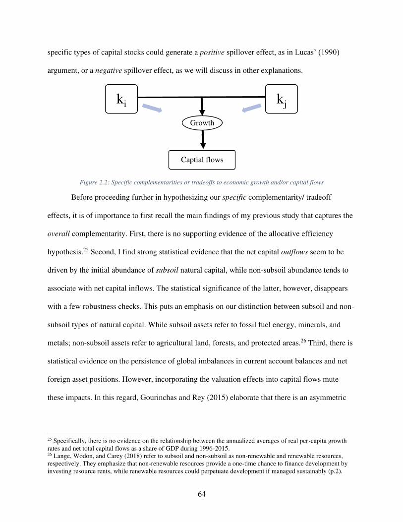
64

specific types of capital stocks could generate a positive spillover effect, as in Lucas’ (1990)

argument, or a negative spillover effect, as we will discuss in other explanations.

Figure 2.2: Specific complementarities or tradeoffs to economic growth and/or capital flows

Before proceeding further in hypothesizing our specific complementarity/ tradeoff

effects, it is of importance to first recall the main findings of my previous study that captures the

overall complementarity. First, there is no supporting evidence of the allocative efficiency

hypothesis.25 Second, I find strong statistical evidence that the net capital outflows seem to be

driven by the initial abundance of subsoil natural capital, while non-subsoil abundance tends to

associate with net capital inflows. The statistical significance of the latter, however, disappears

with a few robustness checks. This puts an emphasis on our distinction between subsoil and non-

subsoil types of natural capital. While subsoil assets refer to fossil fuel energy, minerals, and

metals; non-subsoil assets refer to agricultural land, forests, and protected areas.26 Third, there is

statistical evidence on the persistence of global imbalances in current account balances and net

foreign asset positions. However, incorporating the valuation effects into capital flows mute

these impacts. In this regard, Gourinchas and Rey (2015) elaborate that there is an asymmetric

25 Specifically, there is no evidence on the relationship between the annualized averages of real per-capita growth rates and net total capital flows as a share of GDP during 1996-2015. 26 Lange, Wodon, and Carey (2018) refer to subsoil and non-subsoil as non-renewable and renewable resources, respectively. They emphasize that non-renewable resources provide a one-time chance to finance development by investing resource rents, while renewable resources could perpetuate development if managed sustainably (p.2).

Growth

ki kj

Captial flows

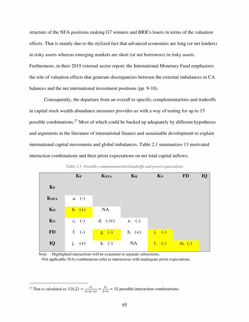
65

structure of the NFA positions making G7 winners and BRICs losers in terms of the valuation

effects. That is mainly due to the stylized fact that advanced economies are long (or net lenders)

in risky assets whereas emerging markets are short (or net borrowers) in risky assets.

Furthermore, in their 2019 external sector report, the International Monetary Fund emphasizes

the role of valuation effects that generate discrepancies between the external imbalances in CA

balances and the net international investment positions (pp. 9-10).

Consequently, the departure from an overall to specific complementarities and tradeoffs

in capital stock wealth abundance measures provides us with a way of testing for up to 15

possible combinations.27 Most of which could be backed up adequately by different hypotheses

and arguments in the literature of international finance and sustainable development to explain

international capital movements and global imbalances. Table 2.1 summarizes 13 motivated

interaction combinations and their priori expectations on net total capital inflows.

Table 2.1: Possible complementarities/tradeoffs and priori expectations

KP KNFA KH KN FD IQ

KP

KNFA a. (-)

KH b. (+) NA

KN c. (-) d. (-/+) e. (-)

FD f. (-) g. (-) h. (+) i. (-)

IQ j. (+) k. (-) NA l. (-) m. (-)

Note: - Highlighted interactions will be examined in separate subsections.

- Not applicable (NA) combinations refer to interactions with inadequate priori expectations.

27 That is calculated as: C(6,2) = 6!2!∗(6−2)! = 6!2!∗4! = 15 possible interaction combinations.

66

The priori expectations, shown in Table 2.1, are hypothesized as follows:

a. Based on the standard neoclassical theory, rich countries should tend to have higher physical

capital abundance and to be net external creditors, so they should associate with net capital

outflows rather than inflows. The interdependency should exacerbate the outflows too.

b. Lucas (1990) demonstrates the paradox and concludes that human capital acts as a positive

spillover, which leads to higher capital inflows. Particularly, the positive spillover effect is

generated by the interdependency between physical capital and human capital.

c. According to the resource curse literature that higher resource-abundant countries could have

higher investment rates but slower growth performance. This could be due to the diminishing

return assumption as in the neoclassical theory or due to other reasons. Nili and Rastad

(2007), for example, find that oil-exporting economies had relatively higher investment rates

but slower growth performance, and attribute that to frictions in their financial systems that

fail to allocate funds to more productive entrepreneurial, rather than rent-seeking, activities.

Thus, given physical capital abundance, I expect an accelerating effect from natural capital

on net capital outflows, as captured by a negative coefficient.

d. As concluded in my previous study, subsoil (non-subsoil) abundant countries tend to be net

external creditors (debtors). Hence, I expect an amplifying negative (positive) effect on net

capital inflows from the higher abundance of subsoil (non-subsoil) natural capital, given

initial external positions.

e. Gylfason (2004) argues that it is all about natural capital that directly and indirectly affects

economic growth. Specifically, he explains the indirect effect through crowding out all other

types of capital stocks including human capital. Thus, I could expect an interdependency

67

between natural capital and human capital that generates a negative spillover and, hence, less

foreign capital flows in.28

f. Given a high physical capital abundance, the higher financial system development could

ensure that funds are efficiently allocated to most productive activities and, hence, reduce the

need for foreign capital inflows.

g. Blecker (2005) explains the persistent global imbalances by arguing for a comparative

advantage in selling financial assets. Deficit CA or net capital importing countries were able

to sustain such positions through their relatively higher degrees of financial system

development. Simply put, given an initial debtor position (NFA<0), the higher degrees of

financial development should associate with larger net capital inflows, as captured by a

negative interaction term.

h. Although the interdependence between human capital and financial development is less clear,

both of which have been identified as absorptive capacities in which the growth impact from

FDI could materialize in a hosting economy. Borensztein, De Gregorio, and Lee (1998) find

a threshold of human capital while Alfaro et al. (2004) find a threshold of financial

development. Therefore, to some extent, I hypothesize that both absorptive capacities should

generate a complementarity to growth and capital inflows.

i. This is similar to the hypothesis (e) on the crowding-out argument by Gylfason (2004). Also,

Beck (2011) discusses a resource curse on financial development. I could hypothesize that as

follows: Natural capital distorts domestic financial development, and such a negative

spillover adversely affects growth rates and capital inflows. Regarding our distinction of

natural capital types, therefore, I expect a negative (positive) direct effect from subsoil (non-

28 It should be noted that Botswana is an exceptional case in which rents were channeled efficiently to accumulate human capital that resulted in one of the highest growing economies.

68

subsoil) natural capital, and a positive direct effect from financial development. Given a high

abundance level of subsoil abundance, we expect a dampening effect from the higher

financial system development on net capital outflows.

j. Acemoglu, Johnson, and Robinson (2001) examine the fundamental causes of growth and

find evidence on the role of institutions; whereas, Alfaro et al. (2008) and Papaioannou

(2009) conclude that the leading factor behind the Lucas' (1990) paradox is intuitional

quality.29 This could also imply that there is a positive growth spillover effect, generated

from physical capital abundance and better institutions, which attracts more capital inflows.

Thus, I could hypothesize that rich economies, in terms of physical abundance, were able to

associate with net capital outflows due to their superior institutions.

k. This hypothesis is closely related to the previous. One the one hand, the standard neoclassical

theory seemed to be irrelevant because it suggests that rich countries should be creditors

rather than debtors. On the other, the empirical observation implies that debtor countries

were able to sustain CA deficit or capital inflows because of their superior institutions.

Following the empirical observation, therefore, I expect a negative main effect from initial

NFA and positive for institutional quality, while the indirect effect should be negative. That

is, given an external debt position (NFA<0), the higher institutional quality, the more capital

should flow in.

l. Gylfason (2004) asserts that it is all about natural capital that adversely affects economic

growth directly and indirectly through crowding out other types of capital stocks, including

social capital (or institutions). While Mehlum, Moene, and Torvik (2006) demonstrate that

resource-dependent countries with only very superior institutions could neutralize the

29 While the focus of Alfaro et al. (2008) is on gross private capital inflows using a cross-section OLS and IV analyses, Papaioannou (2009) adopts a gravity equation analyses using cross-section and panel analyses.

69

resource curse. Hence, given a subsoil (non-subsoil) capital abundance with a negative

(positive) main direct effect on capital inflows, I expect an accelerating (dampening) effect

from the institutional quality on net capital inflows.30

m. Chinn et al. (2014) test the global saving glut argument, introduced by Bernanke (2005), via

interacting not only FD and IQ but also KA openness. Their priori expectation is that lower

values of these variables explain the upstream capital flows from emerging markets and

developing economies (EMDEs) to advanced economies (AEs).

Data and Empirical Approach

2.3.1 Data Sources

I rely on different datasets that collectively cover a sample of 95 countries during 1995-

2015. First, data sources for net total capital inflows include the International Monetary Fund

(IMF)- International Financial Statistics (IFS), Lane and Milesi-Ferretti (2007, 2017) and Alfaro

et al. (2014). There are two main measures of net total capital inflows. The typical measure in the

literature is the reversed sign of the current account balance, and the other adjusts for valuations

of a country’s gross assets and liabilities. The relationship between the two measures is captured

by the fact that the net foreign asset (NFA) position is the sum of cumulative CA surpluses over

the past till present and the valuation effects at the current year, and by applying stock-flow

accounting we get the second measure of net total capital inflows. In short, the typical measure is

(-CA, %GDP) and the valuation-adjusted measure is (-ΔNFA or ΔNFL, %GDP). Data of the

former is available in the IMF-IFS, and the latter is available and constructed by Lane and

Milesi-Ferretti.

30 As discussed earlier, unlike non-subsoil types, subsoil resources provide a one-time chance to finance development (Lange, Wodon, and Carey 2018, p. 33).

70

Other data sources are as follows. Wealth stock measures are available in the World Bank

(WB)- Wealth Accounts database (WA). A proxy for the institutional quality index is

constructed as a composite index using the six sub-indicators available in the International

Country Risk Guide (ICRG).31 These sub-indicators are: 1) Voice and Accountability, 2)

Political Stability and Absence of Violence, 3) Government Effectiveness, 4) Regulatory

Quality, 5) Rule of Law, and 6) Control of Corruption. In addition, I adopt a composite index for

financial system development constructed by Svirydzenka (2016), and the data of which are

available by the IMF. This measure is constructed using a bottom-up approach in three levels.

The composite index of financial system development is constructed from two sub-indicators:

financial institutions and financial markets. Each of these is also constructed from three sub-

indicators regarding depth, access, and efficiency that rely on many financial variables. Finally, I

use a de jure capital account openness index constructed by Chinn and Ito (2006).

2.3.2 Econometric Approach

I employ an OLS regression analysis with robust standard errors while modifying a

specification by Gourinchas and Jeanne (2013). The analysis covers a sample of 95 countries and

spans over 1995-2015. To mitigate endogeneity concerns due to simultaneity bias, I will run the

annualized averages of net capital inflows over 1996-2015 on the lagged initial abundance

measures of capital stocks in 1995. Simply put, I examine the role of initial abundance measures

on the subsequent annualized averages net capital inflows, expressed as %GDP to eliminate the

effects of country-size differences.

To capture the specific complementarities and trade-offs, an interaction effect is included.

I aim is to capture the interdependency of two or more of the wealth abundance components that

31 The composite index is constructed by assigning equal weights to the six indictors, so that it ranges between zero and one.

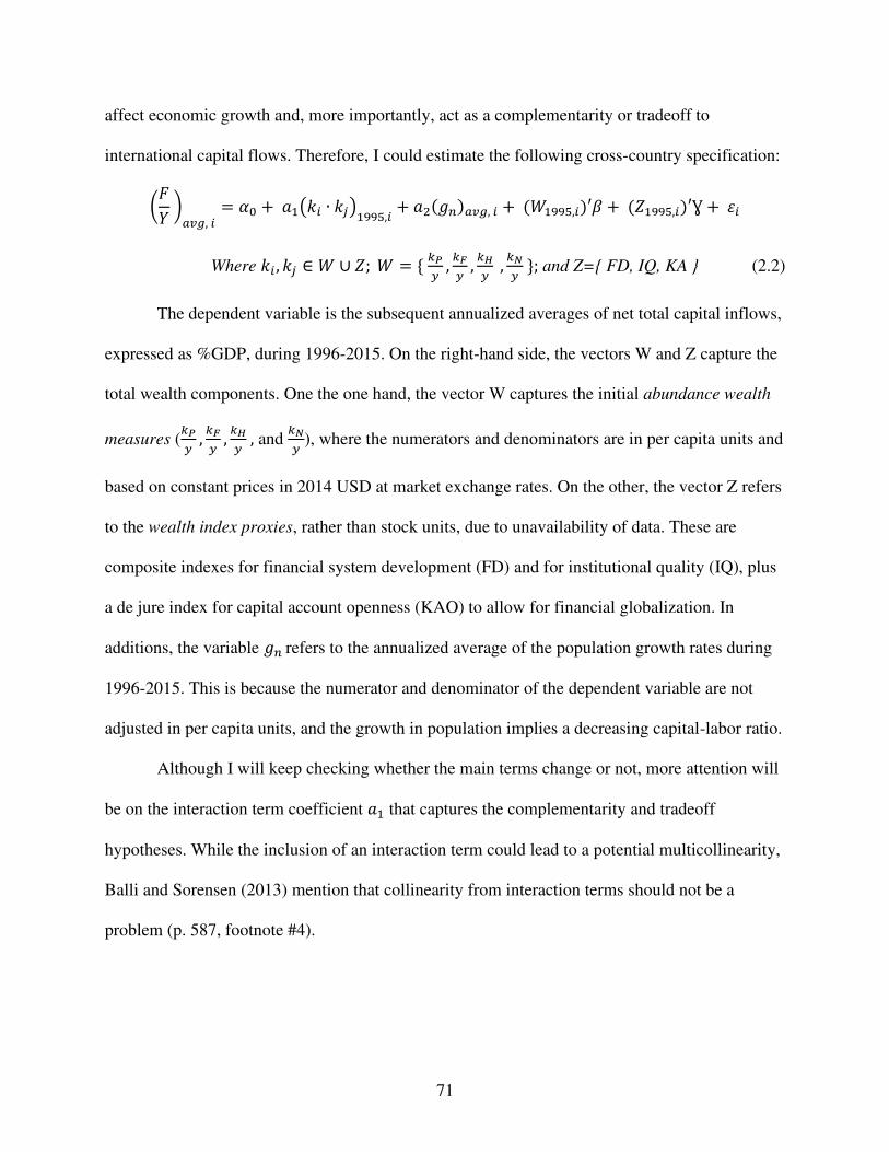
71

affect economic growth and, more importantly, act as a complementarity or tradeoff to

international capital flows. Therefore, I could estimate the following cross-country specification:

(𝐹𝑌 )𝑎𝑣𝑔, 𝑖 = 𝛼0 + 𝑎1(𝑘𝑖 ∙ 𝑘𝑗)1995,𝑖 + 𝑎2(𝑔𝑛)𝑎𝑣𝑔, 𝑖 + (𝑊1995,𝑖)′𝛽 + (𝑍1995,𝑖)′Ɣ + 𝜀𝑖 Where 𝑘𝑖 , 𝑘𝑗 ∈ 𝑊 ∪ 𝑍; 𝑊 = { 𝑘𝑃𝑦 , 𝑘𝐹𝑦 , 𝑘𝐻𝑦 , 𝑘𝑁𝑦 }; and Z={ FD, IQ, KA } (2.2)

The dependent variable is the subsequent annualized averages of net total capital inflows,

expressed as %GDP, during 1996-2015. On the right-hand side, the vectors W and Z capture the

total wealth components. One the one hand, the vector W captures the initial abundance wealth

measures (𝑘𝑃𝑦 , 𝑘𝐹𝑦 , 𝑘𝐻𝑦 , and

𝑘𝑁𝑦 ), where the numerators and denominators are in per capita units and

based on constant prices in 2014 USD at market exchange rates. On the other, the vector Z refers

to the wealth index proxies, rather than stock units, due to unavailability of data. These are

composite indexes for financial system development (FD) and for institutional quality (IQ), plus

a de jure index for capital account openness (KAO) to allow for financial globalization. In

additions, the variable 𝑔𝑛 refers to the annualized average of the population growth rates during

1996-2015. This is because the numerator and denominator of the dependent variable are not

adjusted in per capita units, and the growth in population implies a decreasing capital-labor ratio.

Although I will keep checking whether the main terms change or not, more attention will

be on the interaction term coefficient 𝑎1 that captures the complementarity and tradeoff

hypotheses. While the inclusion of an interaction term could lead to a potential multicollinearity,

Balli and Sorensen (2013) mention that collinearity from interaction terms should not be a

problem (p. 587, footnote #4).

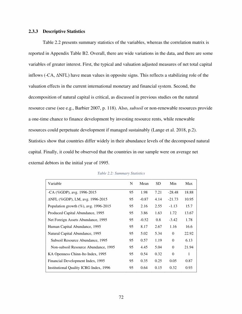
72

2.3.3 Descriptive Statistics

Table 2.2 presents summary statistics of the variables, whereas the correlation matrix is

reported in Appendix Table B2. Overall, there are wide variations in the data, and there are some

variables of greater interest. First, the typical and valuation adjusted measures of net total capital

inflows (-CA, ∆NFL) have mean values in opposite signs. This reflects a stabilizing role of the

valuation effects in the current international monetary and financial system. Second, the

decomposition of natural capital is critical, as discussed in previous studies on the natural

resource curse (see e.g., Barbier 2007, p. 118). Also, subsoil or non-renewable resources provide

a one-time chance to finance development by investing resource rents, while renewable

resources could perpetuate development if managed sustainably (Lange et al. 2018, p.2).

Statistics show that countries differ widely in their abundance levels of the decomposed natural

capital. Finally, it could be observed that the countries in our sample were on average net

external debtors in the initial year of 1995.

Table 2.2: Summary Statistics

Variable N Mean SD Min Max

-CA (%GDP), avg. 1996-2015 95 1.98 7.21 -28.48 18.88

∆NFL (%GDP), LM, avg. 1996-2015 95 -0.87 4.14 -21.73 10.95

Population growth (%), avg. 1996-2015 95 2.16 2.55 -1.13 15.7

Produced Capital Abundance, 1995 95 3.86 1.63 1.72 13.67

Net Foreign Assets Abundance, 1995 95 -0.52 0.8 -3.42 1.78

Human Capital Abundance, 1995 95 8.17 2.67 1.16 16.6

Natural Capital Abundance, 1995 95 5.02 5.34 0 22.92

Subsoil Resource Abundance, 1995 95 0.57 1.19 0 6.13

Non-subsoil Resource Abundance, 1995 95 4.45 5.04 0 21.94

KA Openness Chinn-Ito Index, 1995 95 0.54 0.32 0 1

Financial Development Index, 1995 95 0.35 0.25 0.05 0.87

Institutional Quality ICRG Index, 1996 95 0.64 0.15 0.32 0.93

73

Diagnoses and Empirical Results

Most of the hypotheses could be tested for via interaction terms, but some hypotheses

need some diagnostics and specific treatments when tested. I devote separate subsections for

such hypotheses along with some important ones, while the others will be together discussed

afterward due to space limitations.

2.4.1 Human Capital Externality

Previous studies argue that advanced economies tend to attract capital flows because of

their human capital acting as a positive externality as in Lucas (1990). In this regard, Boz et al.

(2017) interpret that as a complementarity effect between physical capital and human capital.

Thus, I could capture the nonlinear relationship between capital flows and these two types of

capital stocks by a continuous interaction term specification.

First, I should note that the human capital abundance has entered with a puzzling

negative coefficient when not considering an interaction term, and I have raised concerns in a

previous study about the calculation method on whether it captures the quality or the cost of the

labor force. The World Bank’s measure of human capital wealth is based on the Jorgenson-

Fraumeni lifetime earnings approach (1992). Hamilton et al. (2018) state, “Human capital wealth

is defined as the discounted value of future earnings for a country’s labor force” (p. 117).

Specifically, their approach is based on 1) estimating a wage equation regression, and 2)

calibrating the labor share in the national income.32 In a country comparison context, however,

this measure could reflect the cost more than the quality of the labor force. Also, and more

importantly, globalization in trade, and particularly the role of global value chains (GVCs), could

32 Wage is regressed on average years of schooling and experience. The latter is calculated as difference between the working age, on the one hand, and the sum of years of schooling and pre-schooling, on the other hand.

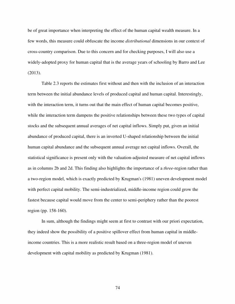
74

be of great importance when interpreting the effect of the human capital wealth measure. In a

few words, this measure could obfuscate the income distributional dimensions in our context of

cross-country comparison. Due to this concern and for checking purposes, I will also use a

widely-adopted proxy for human capital that is the average years of schooling by Barro and Lee

(2013).

Table 2.3 reports the estimates first without and then with the inclusion of an interaction

term between the initial abundance levels of produced capital and human capital. Interestingly,

with the interaction term, it turns out that the main effect of human capital becomes positive,

while the interaction term dampens the positive relationships between these two types of capital

stocks and the subsequent annual averages of net capital inflows. Simply put, given an initial

abundance of produced capital, there is an inverted U-shaped relationship between the initial

human capital abundance and the subsequent annual average net capital inflows. Overall, the

statistical significance is present only with the valuation-adjusted measure of net capital inflows

as in columns 2b and 2d. This finding also highlights the importance of a three-region rather than

a two-region model, which is exactly predicted by Krugman's (1981) uneven development model

with perfect capital mobility. The semi-industrialized, middle-income region could grow the

fastest because capital would move from the center to semi-periphery rather than the poorest

region (pp. 158-160).

In sum, although the findings might seem at first to contrast with our priori expectation,

they indeed show the possibility of a positive spillover effect from human capital in middle-

income countries. This is a more realistic result based on a three-region model of uneven

development with capital mobility as predicted by Krugman (1981).

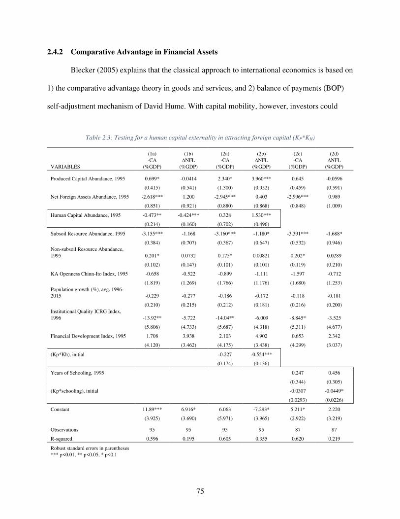
75

2.4.2 Comparative Advantage in Financial Assets

Blecker (2005) explains that the classical approach to international economics is based on

1) the comparative advantage theory in goods and services, and 2) balance of payments (BOP)

self-adjustment mechanism of David Hume. With capital mobility, however, investors could

Table 2.3: Testing for a human capital externality in attracting foreign capital (KP*KH)

(1a) (1b) (2a) (2b) (2c) (2d)

VARIABLES

-CA

(%GDP)

∆NFL

(%GDP)

-CA

(%GDP)

∆NFL

(%GDP)

-CA

(%GDP)

∆NFL

(%GDP)

Produced Capital Abundance, 1995 0.699* -0.0414 2.340* 3.960*** 0.645 -0.0596

(0.415) (0.541) (1.300) (0.952) (0.459) (0.591)

Net Foreign Assets Abundance, 1995 -2.618*** 1.200 -2.945*** 0.403 -2.996*** 0.989

(0.851) (0.921) (0.880) (0.868) (0.848) (1.009)

Human Capital Abundance, 1995 -0.473** -0.424*** 0.328 1.530***

(0.214) (0.160) (0.702) (0.496)

Subsoil Resource Abundance, 1995 -3.155*** -1.168 -3.160*** -1.180* -3.391*** -1.688*

(0.384) (0.707) (0.367) (0.647) (0.532) (0.946)

Non-subsoil Resource Abundance,

1995 0.201* 0.0732 0.175* 0.00821 0.202* 0.0289

(0.102) (0.147) (0.101) (0.101) (0.119) (0.210)

KA Openness Chinn-Ito Index, 1995 -0.658 -0.522 -0.899 -1.111 -1.597 -0.712

(1.819) (1.269) (1.766) (1.176) (1.680) (1.253)

Population growth (%), avg. 1996-

2015 -0.229 -0.277 -0.186 -0.172 -0.118 -0.181

(0.210) (0.215) (0.212) (0.181) (0.216) (0.200)

Institutional Quality ICRG Index,

1996 -13.92** -5.722 -14.04** -6.009 -8.845* -3.525

(5.806) (4.733) (5.687) (4.318) (5.311) (4.677)

Financial Development Index, 1995 1.708 3.938 2.103 4.902 0.653 2.342

(4.120) (3.462) (4.175) (3.438) (4.299) (3.037)

(Kp*Kh), initial -0.227 -0.554***

(0.174) (0.136)

Years of Schooling, 1995 0.247 0.456

(0.344) (0.305)

(Kp*schooling), initial -0.0307 -0.0449*

(0.0293) (0.0226)

Constant 11.89*** 6.916* 6.063 -7.293* 5.211* 2.220

(3.925) (3.690) (5.971) (3.965) (2.922) (3.219)

Observations 95 95 95 95 87 87

R-squared 0.596 0.195 0.605 0.355 0.620 0.219


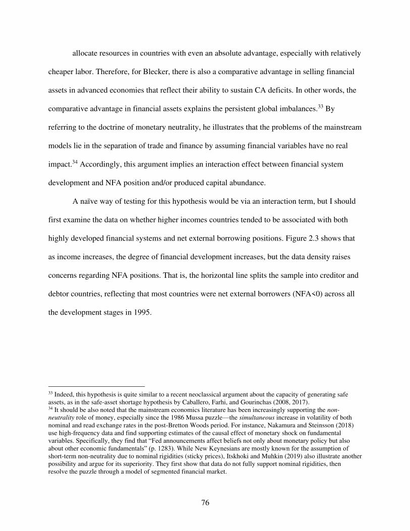
76

allocate resources in countries with even an absolute advantage, especially with relatively

cheaper labor. Therefore, for Blecker, there is also a comparative advantage in selling financial

assets in advanced economies that reflect their ability to sustain CA deficits. In other words, the

comparative advantage in financial assets explains the persistent global imbalances.33 By

referring to the doctrine of monetary neutrality, he illustrates that the problems of the mainstream

models lie in the separation of trade and finance by assuming financial variables have no real

impact.34 Accordingly, this argument implies an interaction effect between financial system

development and NFA position and/or produced capital abundance.

A naïve way of testing for this hypothesis would be via an interaction term, but I should

first examine the data on whether higher incomes countries tended to be associated with both

highly developed financial systems and net external borrowing positions. Figure 2.3 shows that

as income increases, the degree of financial development increases, but the data density raises

concerns regarding NFA positions. That is, the horizontal line splits the sample into creditor and

debtor countries, reflecting that most countries were net external borrowers (NFA<0) across all

the development stages in 1995.

33 Indeed, this hypothesis is quite similar to a recent neoclassical argument about the capacity of generating safe assets, as in the safe-asset shortage hypothesis by Caballero, Farhi, and Gourinchas (2008, 2017). 34 It should be also noted that the mainstream economics literature has been increasingly supporting the non-

neutrality role of money, especially since the 1986 Mussa puzzle—the simultaneous increase in volatility of both nominal and read exchange rates in the post-Bretton Woods period. For instance, Nakamura and Steinsson (2018) use high-frequency data and find supporting estimates of the causal effect of monetary shock on fundamental variables. Specifically, they find that “Fed announcements affect beliefs not only about monetary policy but also about other economic fundamentals” (p. 1283). While New Keynesians are mostly known for the assumption of short-term non-neutrality due to nominal rigidities (sticky prices), Itskhoki and Muhkin (2019) also illustrate another possibility and argue for its superiority. They first show that data do not fully support nominal rigidities, then resolve the puzzle through a model of segmented financial market.

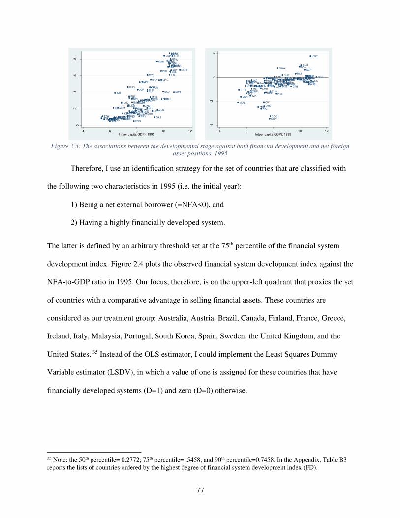
77

Figure 2.3: The associations between the developmental stage against both financial development and net foreign

asset positions, 1995

Therefore, I use an identification strategy for the set of countries that are classified with

the following two characteristics in 1995 (i.e. the initial year):

1) Being a net external borrower (=NFA<0), and

2) Having a highly financially developed system.

The latter is defined by an arbitrary threshold set at the 75th percentile of the financial system

development index. Figure 2.4 plots the observed financial system development index against the

NFA-to-GDP ratio in 1995. Our focus, therefore, is on the upper-left quadrant that proxies the set

of countries with a comparative advantage in selling financial assets. These countries are

considered as our treatment group: Australia, Austria, Brazil, Canada, Finland, France, Greece,

Ireland, Italy, Malaysia, Portugal, South Korea, Spain, Sweden, the United Kingdom, and the

United States. 35 Instead of the OLS estimator, I could implement the Least Squares Dummy

Variable estimator (LSDV), in which a value of one is assigned for these countries that have

financially developed systems (D=1) and zero (D=0) otherwise.

35 Note: the 50th percentile= 0.2772; 75th percentile= .5458; and 90th percentile=0.7458. In the Appendix, Table B3 reports the lists of countries ordered by the highest degree of financial system development index (FD).

PRY

BOL

PER

KENNIC

ECU

IND

ZMB

PHL

THAZAF

CHN

VNM

TGO

PAN

URY

BGD

COG

IDN

SLV

OMNBHR

PAK

NGA

TUR

EGY

GUY

MLI

MAR

DOMPNG

MLT

BFA

MEX

GAB

TUN

CMRYEM

UGA

BGR

MNG

CHL

TZA

JAM

SUR

COL

BWACRI

LBN

SAU

HND

NAM

ETH

NERSEN

POL

MWI

VEN

HUN

CIV

KWT

GTM

LKA

GMBGHA

GINMOZ

SLE

JOR

MDG

ALB

ARG

AUSUSA

DEUSWE

SGP

KOR

DNK

GBRESP

ITA

IRL

AUTPRT

MYS

BEL

FRA

NLD

NOR

BRA GRC

CAN

FIN

JPN

0.2

.4.6

.8


PRY

BOLPER

KEN

NIC

ECU

IND

ZMB

PHL THA

ZAFCHN

VNM

TGO

PAN

URYBGD

COG

IDN

SLVOMN

BHR

PAK

NGA

TUREGY

GUY

MLI

MARDOM

PNG

MLT

BFAMEX

GAB

TUNCMR

YEM

UGABGR

MNG CHL

TZA

JAM

SUR

COL

BWA

CRILBN

SAU

HND

NAM

ETH

NER SEN

POL

MWI

VEN

HUN

CIV

KWT

GTM

LKAGMB

GHAGIN

MOZ

SLE

JOR

MDG

ALBARG

AUS

USADEU

SWE

SGP

KORDNK

GBRESPITA

IRLAUTPRT

MYS

BELFRA

NLD NORBRA GRC

CANFIN

JPN

-4-2

02


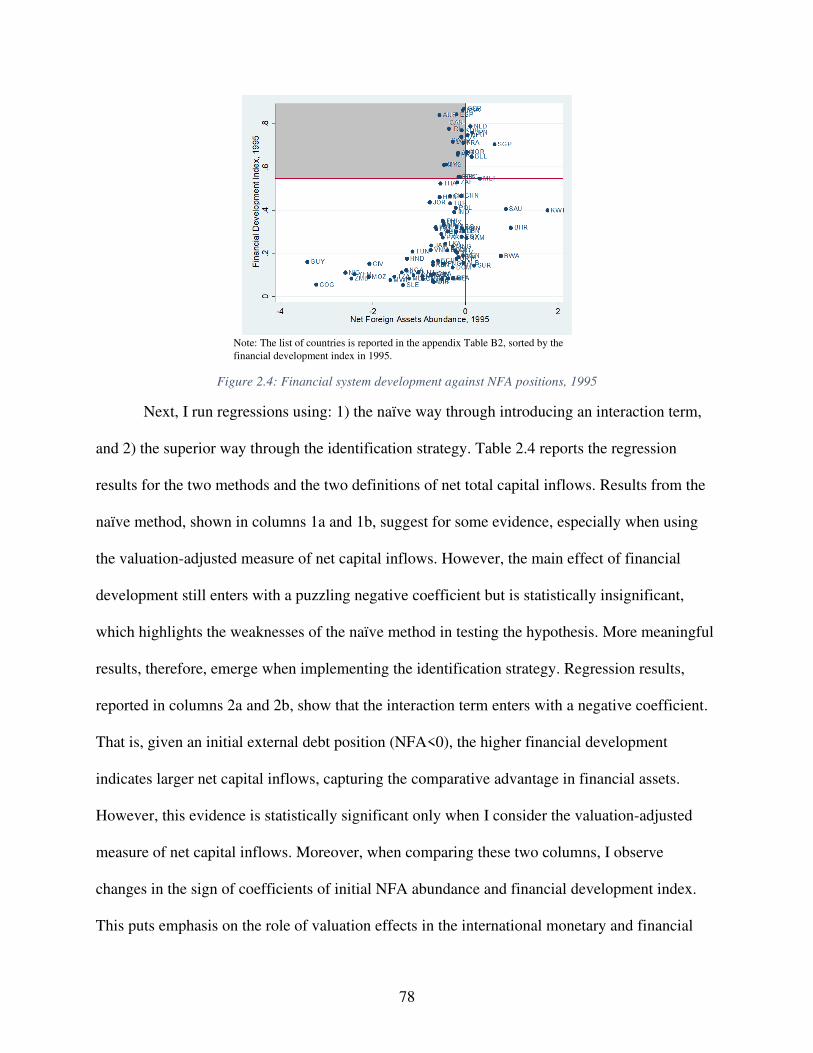
78

Note: The list of countries is reported in the appendix Table B2, sorted by the

financial development index in 1995.

Figure 2.4: Financial system development against NFA positions, 1995

Next, I run regressions using: 1) the naïve way through introducing an interaction term,

and 2) the superior way through the identification strategy. Table 2.4 reports the regression

results for the two methods and the two definitions of net total capital inflows. Results from the

naïve method, shown in columns 1a and 1b, suggest for some evidence, especially when using

the valuation-adjusted measure of net capital inflows. However, the main effect of financial

development still enters with a puzzling negative coefficient but is statistically insignificant,

which highlights the weaknesses of the naïve method in testing the hypothesis. More meaningful

results, therefore, emerge when implementing the identification strategy. Regression results,

reported in columns 2a and 2b, show that the interaction term enters with a negative coefficient.

That is, given an initial external debt position (NFA<0), the higher financial development

indicates larger net capital inflows, capturing the comparative advantage in financial assets.

However, this evidence is statistically significant only when I consider the valuation-adjusted

measure of net capital inflows. Moreover, when comparing these two columns, I observe

changes in the sign of coefficients of initial NFA abundance and financial development index.

This puts emphasis on the role of valuation effects in the international monetary and financial

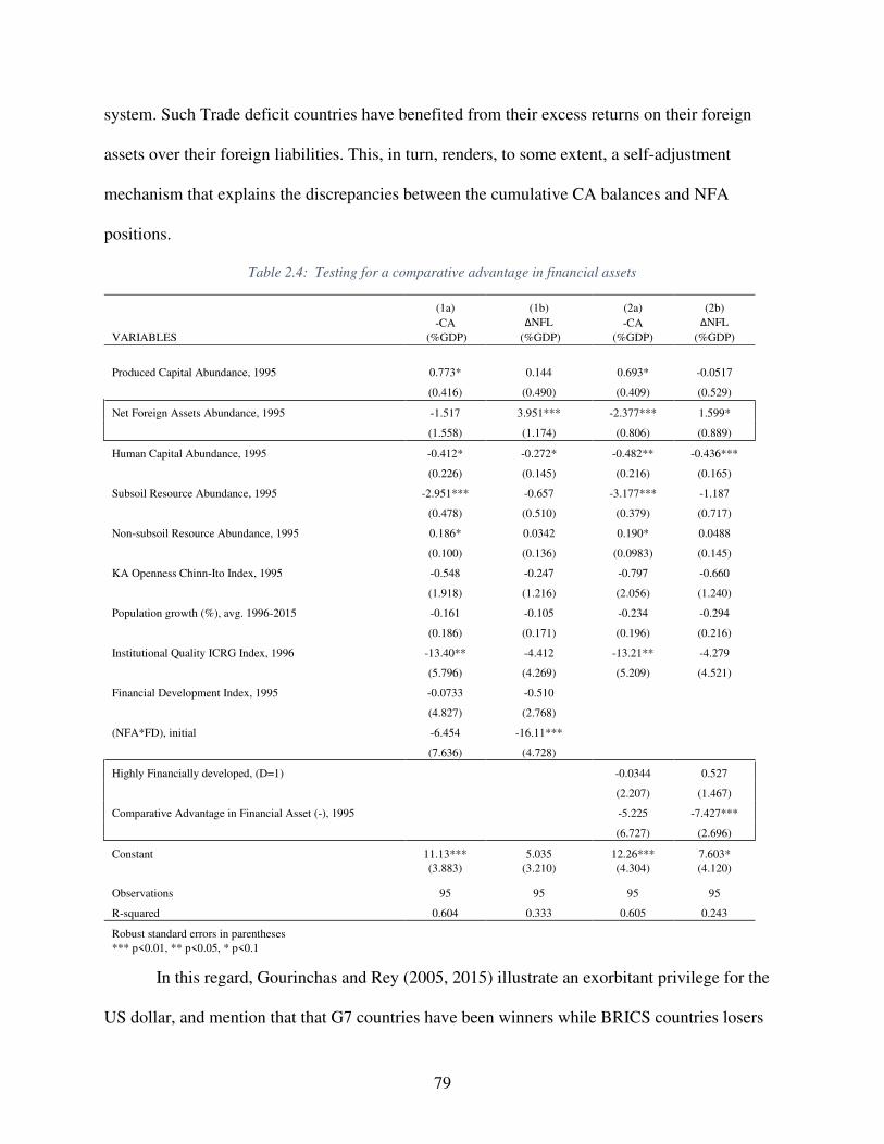
79

system. Such Trade deficit countries have benefited from their excess returns on their foreign

assets over their foreign liabilities. This, in turn, renders, to some extent, a self-adjustment

mechanism that explains the discrepancies between the cumulative CA balances and NFA

positions.

Table 2.4: Testing for a comparative advantage in financial assets

(1a) (1b) (2a) (2b)

VARIABLES

-CA

(%GDP)

∆NFL

(%GDP)

-CA

(%GDP)

∆NFL

(%GDP)

Produced Capital Abundance, 1995 0.773* 0.144 0.693* -0.0517

(0.416) (0.490) (0.409) (0.529)

Net Foreign Assets Abundance, 1995 -1.517 3.951*** -2.377*** 1.599*

(1.558) (1.174) (0.806) (0.889)

Human Capital Abundance, 1995 -0.412* -0.272* -0.482** -0.436***

(0.226) (0.145) (0.216) (0.165)

Subsoil Resource Abundance, 1995 -2.951*** -0.657 -3.177*** -1.187

(0.478) (0.510) (0.379) (0.717)

Non-subsoil Resource Abundance, 1995 0.186* 0.0342 0.190* 0.0488

(0.100) (0.136) (0.0983) (0.145)

KA Openness Chinn-Ito Index, 1995 -0.548 -0.247 -0.797 -0.660

(1.918) (1.216) (2.056) (1.240)

Population growth (%), avg. 1996-2015 -0.161 -0.105 -0.234 -0.294

(0.186) (0.171) (0.196) (0.216)

Institutional Quality ICRG Index, 1996 -13.40** -4.412 -13.21** -4.279

(5.796) (4.269) (5.209) (4.521)

Financial Development Index, 1995 -0.0733 -0.510

(4.827) (2.768)

(NFA*FD), initial -6.454 -16.11***

(7.636) (4.728)

Highly Financially developed, (D=1) -0.0344 0.527

(2.207) (1.467)

Comparative Advantage in Financial Asset (-), 1995 -5.225 -7.427***

(6.727) (2.696)

Constant 11.13*** 5.035 12.26*** 7.603*

(3.883) (3.210) (4.304) (4.120)

Observations 95 95 95 95

R-squared 0.604 0.333 0.605 0.243


In this regard, Gourinchas and Rey (2005, 2015) illustrate an exorbitant privilege for the

US dollar, and mention that that G7 countries have been winners while BRICS countries losers

80

from the valuation adjustments. Gourinchas and Rey (2015) also state, “The valuation channel

has historically accounted for roughly 30% of the process of adjustment of the United States

toward its long-run solvency constraint.” (p. 635) In addition, using a sample of 52 economies

over 1990-2015, Adler and Garcia-Macia (2018) find that the valuation changes are driven by

asset price changes, rather than yield differentials or exchange rate changes.

2.4.3 Global Saving Glut

Chinn et al. (2014) test for the global saving glut hypothesis, introduced by Bernanke

(2005). Their argument is based on interactions between KA Openness (KAO) Financial

Development (FD), and Institutional quality (IQ).36 They call these main variables plus their

interactions as the global saving glut variables. It should also be noted this hypothesis is closely

related to the export-led growth strategy implemented, for example, by emerging Asia.

However, those three main variables are believed to be highly correlated, and so

generating multiple interaction terms in the regression analysis is implausible. Although I agree

with Balli and Sorensen (2013, p.587) that while collinearity from an interaction should not be a

problem, generating multiple interactions could raise severe concerns. The correlations between

the values of the main variables range from about 0.5 to 0.87 (see Table B2 in the appendix).

Thus, introducing three interaction terms out of these variables could be problematic.

Instead of generating interaction terms between these highly correlated variables, I

suggest the use of a principal component analysis (PCA) for two reasons. While it could address

the multicollinearity, it also renders an easier way of testing for this hypothesis. The latter means

36 I should note that the proxies used by Chinn et al. (2014) differ from the those of the current study. First, they proxy financial development by the ratio of private credit to GDP, whereas I use the composite broad index of the financial system development introduced by Svirydzenka (2016). Second, they construct an index for institutional quality based on three sub-indicators: law and order, bureaucratic quality, and anti-corruption. However, I construct the index using six sub-indicators as discussed earlier in data section. Both of which, therefore, represent an improvement of the current study over the proxy choices.

81

that I could interpret only one coefficient instead of six. In this procedure, I consider creating a

principal component based on two considerations: i) using only the first three variables (IQ, FD,

and KAO), and ii) the three main variables plus their three interaction terms.

To justify whether the implementation of PCA is appropriate with our data, I conduct the

following investigation. First, by employing a PCA using the three variables (IQ, FD, and KAO)

results suggest that only the first principal component has an eigenvalue greater than one (=2.32),

which captures the maximal overall variance. In simple words, the first component explains

about 77.5% (2.32/3) of the total variance. Also, the values of the factor-loadings are high

ranging from about 0.5 to 0.6. I next employ the Kaiser-Meyer-Olkin (KMO) measure of

sampling adequacy (MSA) and find a justification for using the PCA. Kaiser and Rice (1974)

suggest that a value of 0.5 or less is unacceptable. Specifically, I find the KMO-MSA index is

around 0.62 that is greater than the minimum requirement of 0.5.

Second, by repeating the PCA but for the total of six variables (IQ, FD, KAO, and their

interaction terms), I find similar qualitative results. Particularly, I only find the first component

with an eigenvalue greater that one (=5.06); whereas, the factor-loadings range from about 0.36

to 0.44. Also, the KMO-MSA index is equal to 0.7>0.5, justifying the use of PCA.

Therefore, there is adequate support for the use of PCA in testing for the global saving

glut argument by focusing on the same variables as in Chinn, Eichengreen, and Ito (2014).

Hence, I could control for the first component, which explains much of the variations in the

global saving glut variables.

Table 2.5 columns 1a-2b show regression estimates when control for the first principal

component while contrasting the two measures of net total capital inflows. The coefficient on the

first component enters with an unexpected sign, implying that less-developed counties (in terms

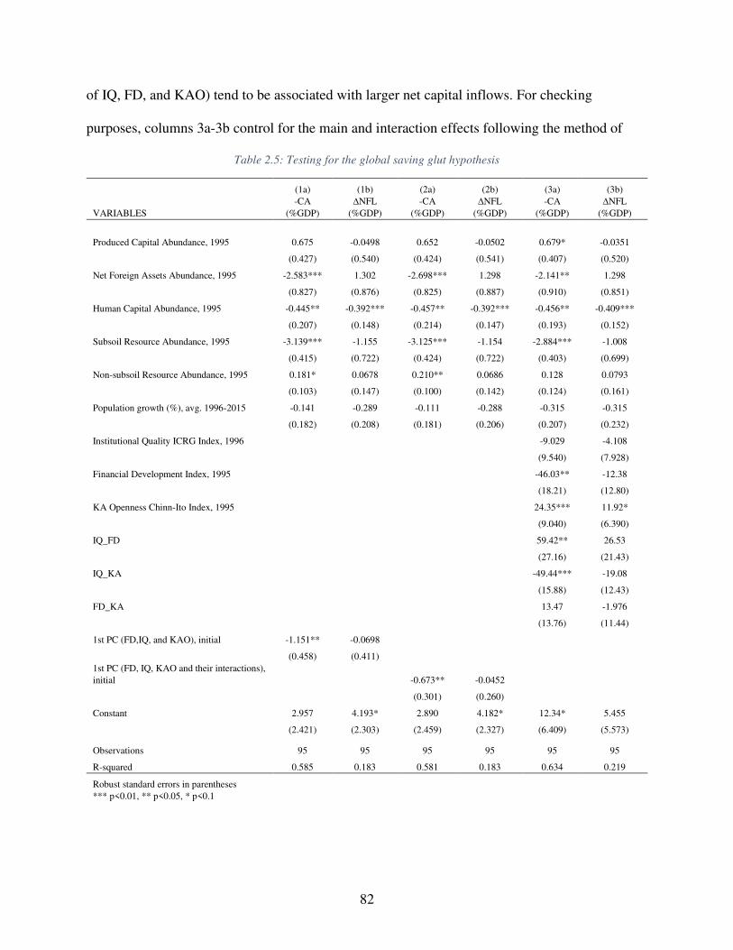
82

of IQ, FD, and KAO) tend to be associated with larger net capital inflows. For checking

purposes, columns 3a-3b control for the main and interaction effects following the method of

Table 2.5: Testing for the global saving glut hypothesis

(1a) (1b) (2a) (2b) (3a) (3b)

VARIABLES

-CA

(%GDP)

∆NFL

(%GDP)

-CA

(%GDP)

∆NFL

(%GDP)

-CA

(%GDP)

∆NFL

(%GDP)

Produced Capital Abundance, 1995 0.675 -0.0498 0.652 -0.0502 0.679* -0.0351

(0.427) (0.540) (0.424) (0.541) (0.407) (0.520)

Net Foreign Assets Abundance, 1995 -2.583*** 1.302 -2.698*** 1.298 -2.141** 1.298

(0.827) (0.876) (0.825) (0.887) (0.910) (0.851)

Human Capital Abundance, 1995 -0.445** -0.392*** -0.457** -0.392*** -0.456** -0.409***

(0.207) (0.148) (0.214) (0.147) (0.193) (0.152)

Subsoil Resource Abundance, 1995 -3.139*** -1.155 -3.125*** -1.154 -2.884*** -1.008

(0.415) (0.722) (0.424) (0.722) (0.403) (0.699)

Non-subsoil Resource Abundance, 1995 0.181* 0.0678 0.210** 0.0686 0.128 0.0793

(0.103) (0.147) (0.100) (0.142) (0.124) (0.161)

Population growth (%), avg. 1996-2015 -0.141 -0.289 -0.111 -0.288 -0.315 -0.315

(0.182) (0.208) (0.181) (0.206) (0.207) (0.232)

Institutional Quality ICRG Index, 1996 -9.029 -4.108

(9.540) (7.928)

Financial Development Index, 1995 -46.03** -12.38

(18.21) (12.80)

KA Openness Chinn-Ito Index, 1995 24.35*** 11.92*

(9.040) (6.390)

IQ_FD 59.42** 26.53

(27.16) (21.43)

IQ_KA -49.44*** -19.08

(15.88) (12.43)

FD_KA 13.47 -1.976

(13.76) (11.44)

1st PC (FD,IQ, and KAO), initial -1.151** -0.0698

(0.458) (0.411) 1st PC (FD, IQ, KAO and their interactions),

initial -0.673** -0.0452

(0.301) (0.260)

Constant 2.957 4.193* 2.890 4.182* 12.34* 5.455

(2.421) (2.303) (2.459) (2.327) (6.409) (5.573)


R-squared 0.585 0.183 0.581 0.183 0.634 0.219


*** p<0.01, ** p<0.05, * p<0.1

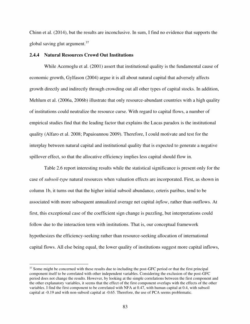
83

Chinn et al. (2014), but the results are inconclusive. In sum, I find no evidence that supports the

global saving glut argument.37

2.4.4 Natural Resources Crowd Out Institutions

While Acemoglu et al. (2001) assert that institutional quality is the fundamental cause of

economic growth, Gylfason (2004) argue it is all about natural capital that adversely affects

growth directly and indirectly through crowding out all other types of capital stocks. In addition,

Mehlum et al. (2006a, 2006b) illustrate that only resource-abundant countries with a high quality

of institutions could neutralize the resource curse. With regard to capital flows, a number of

empirical studies find that the leading factor that explains the Lucas paradox is the institutional

quality (Alfaro et al. 2008; Papaioannou 2009). Therefore, I could motivate and test for the

interplay between natural capital and institutional quality that is expected to generate a negative

spillover effect, so that the allocative efficiency implies less capital should flow in.

Table 2.6 report interesting results while the statistical significance is present only for the

case of subsoil-type natural resources when valuation effects are incorporated. First, as shown in

column 1b, it turns out that the higher initial subsoil abundance, ceteris paribus, tend to be

associated with more subsequent annualized average net capital inflow, rather than outflows. At

first, this exceptional case of the coefficient sign change is puzzling, but interpretations could

follow due to the interaction term with institutions. That is, our conceptual framework

hypothesizes the efficiency-seeking rather than resource-seeking allocation of international

capital flows. All else being equal, the lower quality of institutions suggest more capital inflows,

37 Some might be concerned with these results due to including the post-GFC period or that the first principal component itself to be correlated with other independent variables. Considering the exclusion of the post-GFC period does not change the results. However, by looking at the simple correlations between the first component and the other explanatory variables, it seems that the effect of the first component overlaps with the effects of the other variables. I find the first component to be correlated with NFA at 0.47, with human capital at 0.4, with subsoil capital at -0.19 and with non-subsoil capital at -0.65. Therefore, the use of PCA seems problematic.

84

and the interaction amplifies the relationship. This could mean the foreign investors are more

likely resource-seeking rather than efficiency-seeking. Consequently, this finding captures the

rent-seeking explanation of the natural resource curse phenomenon. Further, the larger net capital

inflows imply an appreciation in the exchange rate, so the Dutch disease effects are more likely

to materialize in the hosting economy. Accordingly, the two known explanations of the resource

curse phenomenon, the rent-seeking activities and Dutch Disease effects, are inferred and

seemed to be somehow related to our empirical analysis of international capital flows.

Table 2.6: Testing for KN*IQ

(1a) (1b) (2a) (2b)

VARIABLES -CA (%GDP) ∆NFL (%GDP) -CA (%GDP) ∆NFL (%GDP)

Produced Capital Abundance, 1995 0.715* 0.0627 0.717* -0.0915

(0.418) (0.530) (0.424) (0.521)

Net Foreign Assets Abundance, 1995 -2.529*** 1.776** -2.605*** 1.163

(0.909) (0.716) (0.857) (0.903)

Human Capital Abundance, 1995 -0.468** -0.391*** -0.479** -0.408***

(0.212) (0.146) (0.214) (0.153)

Subsoil Resource Abundance, 1995 -2.117 5.522** -3.156*** -1.164

(1.806) (2.262) (0.385) (0.732)

Non-subsoil Resource Abundance, 1995 0.198* 0.0504 0.397 -0.472

(0.104) (0.151) (0.406) (0.435)

KA Openness Chinn-Ito Index, 1995 -0.527 0.322 -0.758 -0.243

(1.857) (1.216) (1.896) (1.365)


(0.209) (0.149) (0.209) (0.207)

Institutional Quality ICRG Index, 1996 -13.04** -0.0154 -12.35 -10.10*

(5.913) (3.825) (7.631) (5.578)

Financial Development Index, 1995 1.169 0.462 1.112 5.594

(4.244) (2.578) (4.502) (3.683)

(IQ*subsoil), initial -1.879 -12.11**

(3.287) (4.611)

(IQ*non-subsoil), initial -0.373 1.036

(0.775) (0.879)

Constant 11.39*** 3.735 11.17** 8.905**

(3.868) (3.004) (4.522) (3.886)


R-squared 0.597 0.323 0.597 0.211


85

Differently put, and more interesting, given an abundance level of subsoil capital, only

countries with superior institutions tend to be associated with net capital outflows on average.

Consequently, this suggests that subsoil-abundant countries with superior institutions are better

able to ameliorate the appreciation pressures in the exchange rates, which help mitigate the

Dutch disease effects. Further, it implies that they care about intergenerational welfare in which

they smooth the use of resource windfalls. In short, only countries with both subsoil resource

abundance and high institutional quality, ceteris paribus, tend to associate with higher net capital

outflows on average.

All in all, such findings suggest the importance of differentiating between efficiency-

seeking capital flows, as hypothesized in our unified conceptual framework, and resource-

seeking capital flows. Important policy implications are as follows. Subsoil-rich abundant

countries should smooth the use of resource windfalls through foreign reserve management.

They should also avoid resource-seeking foreign capital inflows. By doing so, they could

ameliorate the appreciation pressures in the exchange rates and, hence, mitigate the Dutch

disease effects.

2.4.5 Natural Resource Curse in Finance

Similar to Gylfason's (2004) argument on crowding-out effects, Beck (2011) finds

empirical evidence of the so-called “a resource curse in financial development”. In a few words,

this is about natural resource-abundant countries that are known to lack development in their

financial systems. To some extent, this argument is also related to another that suggests investing

rents abroad helps mitigate the macroeconomic volatility effects due to volatile world

commodity prices. Commodity-export prices are volatile in international markets, so to mitigate

the volatility impact countries need more developed financial systems. However, resource-rich

86

countries lack financial market development which is one of the explanations for the resource

curse. Besides, windfalls from a resource boom lead to unsustainable consumption levels. To

avoid that, countries could invest in international assets that pay annuities to break out the

unsustainable overconsumption argument (Van der Ploeg and Poelhekke 2009; Rodriguez and

Sachs 1999). Empirically, Beck (2011) finds that natural capital crowds out the development of

financial systems. He concludes that banks in resource-based countries “engage less in

intermediation with the real economy” (p. 24). Moreover, he attributes the underdevelopment of

finance to supply-side, rather than demand-side, constraints that affect firms more than

households.

All the above arguments, therefore, imply an interdependency between financial system

development and natural capital abundance. Thus, our priori expectation is as follows: the

negative spillover effect, generated by the interaction between natural capital and financial

development, should attract little capital inflows or even causes net capital outflows.

Table 2.7 reports the regression results with the decomposition of natural capital

abundance into the subsoil and non-subsoil resources. First, the interaction between subsoil

abundance and financial development seems to matter, especially with the valuation-adjusted net

capital inflows as in column 1b. It turns out that the main effect of subsoil abundance becomes

positive and significant, while the interaction enters negatively with statistical and economic

significance. Conversely, column 2b shows that the main effect of non-subsoil abundance

becomes negatively and statistically insignificant while the indirect effect is significantly

positive, suggesting mixed results for the case non-subsoil resources. Overall findings show

some weakly supporting evidence but only for subsoil types.

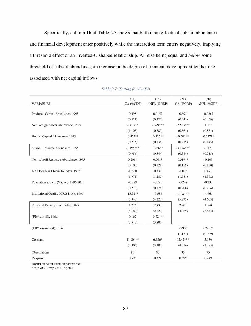
87

Specifically, column 1b of Table 2.7 shows that both main effects of subsoil abundance

and financial development enter positively while the interaction term enters negatively, implying

a threshold effect or an inverted-U shaped relationship. All else being equal and below some

threshold of subsoil abundance, an increase in the degree of financial development tends to be

associated with net capital inflows.

Table 2.7: Testing for KN*FD

(1a) (1b) (2a) (2b)

VARIABLES -CA (%GDP) ∆NFL (%GDP) -CA (%GDP) ∆NFL (%GDP)

Produced Capital Abundance, 1995 0.698 0.0152 0.693 -0.0267

(0.421) (0.521) (0.441) (0.469)

Net Foreign Assets Abundance, 1995 -2.637** 2.329*** -2.563*** 1.067

(1.105) (0.689) (0.861) (0.884)

Human Capital Abundance, 1995 -0.475** -0.327** -0.501** -0.357**

(0.215) (0.136) (0.215) (0.145)

Subsoil Resource Abundance, 1995 -3.195*** 1.226** -3.154*** -1.170

(0.956) (0.544) (0.384) (0.715)

Non-subsoil Resource Abundance, 1995 0.201* 0.0617 0.319** -0.209

(0.103) (0.128) (0.159) (0.130)

KA Openness Chinn-Ito Index, 1995 -0.680 0.830 -1.072 0.471

(1.971) (1.285) (1.981) (1.392)


(0.213) (0.178) (0.206) (0.204)

Institutional Quality ICRG Index, 1996 -13.92** -5.684 -14.24** -4.966

(5.843) (4.227) (5.835) (4.603)

Financial Development Index, 1995 1.726 2.833 2.901 1.080

(4.188) (2.727) (4.389) (3.643)

(FD*subsoil), initial 0.162 -9.724**

(3.543) (3.807)

(FD*non-subsoil), initial -0.930 2.228**

(1.173) (0.909)

Constant 11.90*** 6.186* 12.42*** 5.636

(3.905) (3.303) (4.016) (3.395)


R-squared 0.596 0.324 0.599 0.249


88

2.4.6 Results of Other Hypotheses

Contrary to the standard neoclassical priori expectations, estimates in columns A1 and

A2 of Table 2.8 show a reinforcement of both phenomena: the upstream capital flows and global

imbalances. First, on average rich countries, in terms of physical capital abundance, tend to be

associated with more net capital inflows, as captured by the positive coefficient. Second, the

coefficient on initial NFA is negative, suggesting that creditor (debtor) countries in 1995 have

continued being creditors (debtors). This contrasts with the classical self-adjustment mechanism.

Finally, and more importantly, the interaction term provides evidence of an amplifying effect

against the neoclassical prediction. In other words, external creditors, rich countries have

associated, on average, with increasingly larger net capital inflows.

Regarding the interaction between natural capital and physical capital, columns

C1-4 of Table 2.8 reports the estimates. Results indicate that there is a dampening effect between

the negative (positive) association between initial subsoil (non-subsoil) abundance and

subsequent annualized average net capital inflows. However, the coefficient on the interaction

term is at best of weak statistical significance at the 10% level.

Moreover, columns D1-D4 of Table 2.8 show that the coefficient on the interaction term

of the initial levels of natural resource abundance and NFA is only significant when considering

the valuation-adjusted measure of net capital inflows. This supports our hypothesis and indicates

that an amplifying negative (positive) relationship between initial subsoil (non-subsoil)

abundance and subsequent annualized average net capital inflows.

As predicted by Gylfason (2004), one channel of the resource curse is that natural

resource crowds out human capital. In this study, therefore, I expect the negative spillover effect

89

to be associated with larger net capital outflows. However, results shown in columns E1-4 of

table 9 are still puzzling because the main effect of human capital enters negatively.

Furthermore, results regarding the direct and indirect effect from financial development

and physical capital abundance, as shown in columns F1-2 of Table 2.9, are insignificant. Next,

results pertaining to the main and interaction effects of financial development and human capital

are shown in column H1-2. The main effects still enter with counter-intuitively negative signs

while only the interaction term enters positive as expected. Since these estimates are puzzling, I

find inconclusive evidence. Moving on to the hypothesis of the interdependency between initial

physical abundance and institutional quality, results are reported in columns J1-2. The

coefficients on the main and interaction effects are all statistically insignificant.

Finally, the estimates for the interdependency between the initial institutional quality and

NFA position are reported in columns K1-2 of Table 2.9. However, the direct effect of

institutional quality still enters with an unexpected negative sign, suggesting the results are

inconclusive.

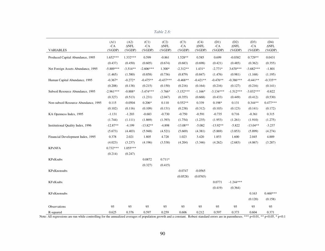
90

Table 2.8:

(A1) (A2) (C1) (C2) (C3) (C4) (D1) (D2) (D3) (D4)

VARIABLES

-CA

(%GDP)

∆NFL

(%GDP)

-CA

(%GDP)

∆NFL

(%GDP)

-CA

(%GDP)

∆NFL

(%GDP)

-CA

(%GDP)

∆NFL

(%GDP)

-CA

(%GDP)

∆NFL

(%GDP)

Produced Capital Abundance, 1995 1.652*** 1.332*** 0.599 -0.861 1.528** 0.585 0.699 -0.0382 0.729** 0.0431

(0.437) (0.450) (0.605) (0.674) (0.683) (0.698) (0.421) (0.485) (0.362) (0.355)

Net Foreign Assets Abundance, 1995 -5.889*** -3.514** -2.606*** 1.300* -2.312** 1.431* -2.771* 3.670*** -3.682*** -1.801

(1.465) (1.580) (0.858) (0.736) (0.879) (0.847) (1.476) (0.981) (1.168) (1.195)

Human Capital Abundance, 1995 -0.367* -0.272* -0.475** -0.437*** -0.468** -0.421** -0.476** -0.386*** -0.441** -0.335**

(0.208) (0.138) (0.215) (0.150) (0.216) (0.164) (0.216) (0.127) (0.216) (0.141)

Subsoil Resource Abundance, 1995 -2.961*** -0.888* -3.474*** -3.766* -3.152*** -1.166* -3.134*** -1.512*** -3.032*** -0.822

(0.327) (0.513) (1.231) (2.047) (0.355) (0.668) (0.433) (0.449) (0.412) (0.530)

Non-subsoil Resource Abundance, 1995 0.115 -0.0504 0.206* 0.110 0.552** 0.339 0.198* 0.131 0.344** 0.477***

(0.102) (0.116) (0.109) (0.131) (0.238) (0.312) (0.103) (0.123) (0.141) (0.172)

KA Openness Index, 1995 -1.131 -1.203 -0.683 -0.730 -0.750 -0.591 -0.735 0.716 -0.361 0.315

(1.744) (1.111) (1.869) (1.393) (1.754) (1.235) (1.953) (1.261) (1.910) (1.275)

Institutional Quality Index, 1996 -12.87** -4.199 -13.82** -4.898 -13.08** -5.082 -13.92** -5.822 -13.04** -3.237

(5.673) (4.403) (5.948) (4.521) (5.669) (4.381) (5.869) (3.853) (5.899) (4.274)

Financial Development Index, 1995 0.378 2.021 1.805 4.728 1.023 3.420 1.853 1.600 2.045 4.889

(4.023) (3.237) (4.196) (3.538) (4.204) (3.346) (4.262) (2.683) (4.067) (3.287)

KPxNFA 0.732*** 1.055***

(0.214) (0.247)

KPxKsubs 0.0872 0.711*

(0.327) (0.415)

KPxKnonsubs -0.0747 -0.0565

(0.0528) (0.0765)

KFxKsubs 0.0771 -1.244***

(0.419) (0.364)

KFxKnonsubs 0.163 0.460***

(0.120) (0.158)

Observations 95 95 95 95 95 95 95 95 95 95

R-squared 0.625 0.376 0.597 0.259 0.606 0.212 0.597 0.373 0.604 0.371

Note: All regressions are run while controlling for the annualized averages of population growth and a constant. Robust standard errors are in parentheses. *** p<0.01, ** p<0.05, * p<0.1

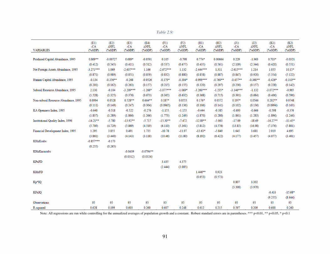
91

Table 2.9:

Note: All regressions are run while controlling for the annualized averages of population growth and a constant. Robust standard errors are in parentheses. *** p<0.01, ** p<0.05, * p<0.1

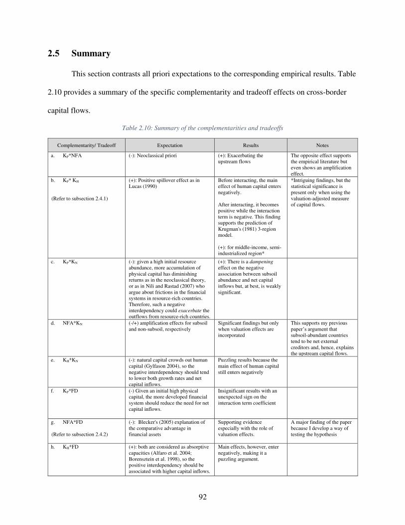
92

Summary

This section contrasts all priori expectations to the corresponding empirical results. Table

2.10 provides a summary of the specific complementarity and tradeoff effects on cross-border

capital flows.

Table 2.10: Summary of the complementarities and tradeoffs

Complementarity/ Tradeoff Expectation Results Notes

a. KP*NFA (-): Neoclassical priori (+): Exacerbating the upstream flows

The opposite effect supports the empirical literature but even shows an amplification effect.

b. KP* KH (Refer to subsection 2.4.1)

(+): Positive spillover effect as in Lucas (1990)

Before interacting, the main effect of human capital enters negatively. After interacting, it becomes positive while the interaction term is negative. This finding supports the prediction of Krugman's (1981) 3-region model. (+): for middle-income, semi-industrialized region*

*Intriguing findings, but the statistical significance is present only when using the valuation-adjusted measure of capital flows.

c. KP*KN (-): given a high initial resource abundance, more accumulation of physical capital has diminishing returns as in the neoclassical theory, or as in Nili and Rastad (2007) who argue about frictions in the financial systems in resource-rich countries. Therefore, such a negative interdependency could exacerbate the outflows from resource-rich countries.

(+): There is a dampening effect on the negative association between subsoil abundance and net capital inflows but, at best, is weakly significant.

d. NFA*KN (-/+) amplification effects for subsoil and non-subsoil, respectively

Significant findings but only when valuation effects are incorporated

This supports my previous paper’s argument that subsoil-abundant countries tend to be net external creditors and, hence, explains the upstream capital flows.

e. KH*KN (-): natural capital crowds out human capital (Gylfason 2004), so the negative interdependency should tend to lower both growth rates and net capital inflows.

Puzzling results because the main effect of human capital still enters negatively

f. KP*FD (-) Given an initial high physical capital, the more developed financial system should reduce the need for net capital inflows.

Insignificant results with an unexpected sign on the interaction term coefficient

g. NFA*FD

(Refer to subsection 2.4.2)

(-): Blecker's (2005) explanation of the comparative advantage in financial assets

Supporting evidence especially with the role of valuation effects.

A major finding of the paper because I develop a way of testing the hypothesis

h. KH*FD (+): both are considered as absorptive capacities (Alfaro et al. 2004; Borensztein et al. 1998), so the positive interdependency should be associated with higher capital inflows.

Main effects, however, enter negatively, making it a puzzling argument.

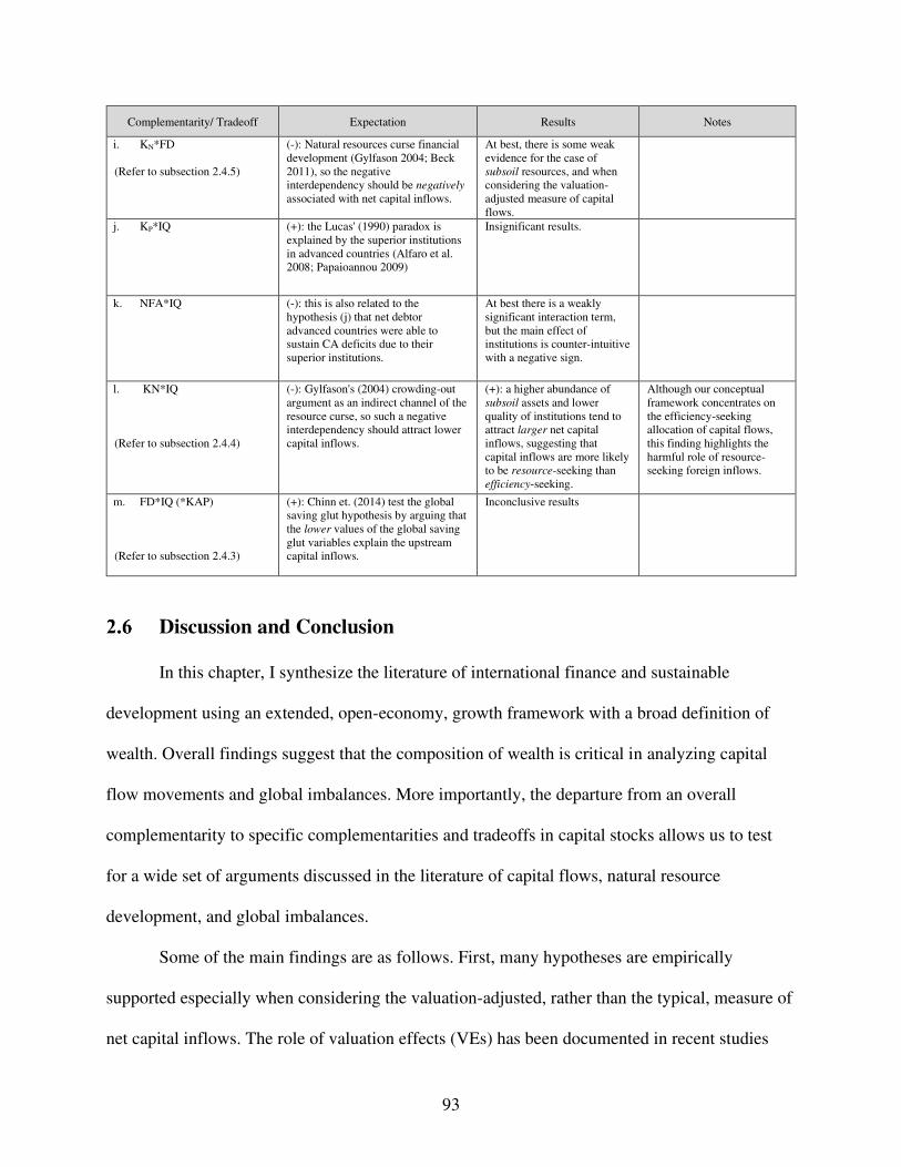
93

Complementarity/ Tradeoff Expectation Results Notes

i. KN*FD (Refer to subsection 2.4.5)

(-): Natural resources curse financial development (Gylfason 2004; Beck 2011), so the negative interdependency should be negatively associated with net capital inflows.

At best, there is some weak evidence for the case of subsoil resources, and when considering the valuation-adjusted measure of capital flows.

j. KP*IQ (+): the Lucas' (1990) paradox is explained by the superior institutions in advanced countries (Alfaro et al. 2008; Papaioannou 2009)

Insignificant results.

k. NFA*IQ (-): this is also related to the hypothesis (j) that net debtor advanced countries were able to sustain CA deficits due to their superior institutions.

At best there is a weakly significant interaction term, but the main effect of institutions is counter-intuitive with a negative sign.

l. KN*IQ (Refer to subsection 2.4.4)

(-): Gylfason's (2004) crowding-out argument as an indirect channel of the resource curse, so such a negative interdependency should attract lower capital inflows.

(+): a higher abundance of subsoil assets and lower quality of institutions tend to attract larger net capital inflows, suggesting that capital inflows are more likely to be resource-seeking than efficiency-seeking.

Although our conceptual framework concentrates on the efficiency-seeking allocation of capital flows, this finding highlights the harmful role of resource-seeking foreign inflows.

m. FD*IQ (*KAP) (Refer to subsection 2.4.3)

(+): Chinn et. (2014) test the global saving glut hypothesis by arguing that the lower values of the global saving glut variables explain the upstream capital inflows.

Inconclusive results


In this chapter, I synthesize the literature of international finance and sustainable

development using an extended, open-economy, growth framework with a broad definition of

wealth. Overall findings suggest that the composition of wealth is critical in analyzing capital

flow movements and global imbalances. More importantly, the departure from an overall

complementarity to specific complementarities and tradeoffs in capital stocks allows us to test

for a wide set of arguments discussed in the literature of capital flows, natural resource

development, and global imbalances.

Some of the main findings are as follows. First, many hypotheses are empirically

supported especially when considering the valuation-adjusted, rather than the typical, measure of

net capital inflows. The role of valuation effects (VEs) has been documented in recent studies

94

and even in the IMF periodical reports (Gourinchas and Rey 2015; Adler and Garcia-Macia

2018; International Monetary Fund 2019a). For instance, the 2019 IMF external sector report

shows that the post-period of 2008-9 global financial crisis (GFC), imbalances in the CAs have

narrowed but increased in the NFA positions. While the former mostly captures the trade

channel, the latter is about the increasingly important role of valuation effects. Second, I find

evidence on an amplification effect that external debtor countries with high physical abundance

in 1995 tend to be associated with annualized average net capital inflows, rather than outflows,

over the subsequent two decades. This contradicts the standard neoclassical theory prediction

that capital should flow to capital-scarce economies. In a few words, this finding shows

supporting evidence on the allocation puzzle against the neoclassical allocative efficiency. Third,

human capital seems to generate an externality that affects capital flows, but it seems to hold as

an inverted U-shaped relationship. This indicates the positive spillover effect from human capital

is of great importance to semi-industrial, middle-income countries. Indeed, Krugman (1981)

predicts that based on his uneven development model when considering a three-region world

with perfect capital mobility. In addition, this evidence supports the arguments about global

value chains in which multinational corporations operate in fragmented production processes to

minimize the cost of their final products. In other words, they could even exploit absolute rather

than comparative advantages worldwide. Indeed, Palley (2015) insists on the role of global value

chains (GVCs), which he particularly describes as “barge economics”, to explain the persistent

global imbalances. He elaborates and criticizes the mainstream explanations for global

imbalances because they are based on the claim of “large benefits from neoliberal globalization”

(p. 47). Fourth, I motivate a way of testing for Blecker's (2005) argument of the comparative

advantage in financial assets, and find supporting evidence especially when valuation effects are

95

incorporated. Consequently, all these explanations indicate that the persistent global imbalances

phenomenon is inevitable in the current international monetary and financial system (IMFS).

The sustainable open-economy growth framework with the broad definition of wealth,

utilized in the current study, helps us better understand the current IMFS. Financial globalization

provides benefits and harms to individual economies and the global economy. For instance, the

IMF analyzes global imbalances based on two components: healthy and risky (see, Obstfeld

2017; International Monetary Fund 2019). The overall findings of the current study put emphasis

on the role of wealth composition when analyzing sustainable economic development and

international financial linkages.

The findings of this chapter, therefore, could suggest different policy implications for i)

advanced economies (AEs) with CA deficits, ii) resource-rich countries, and iii) other emerging

markets and developing economies (EMDEs) especially those with excess-savings. First, AEs

with both CA deficits and highly developed financial systems have benefited from the current

international monetary and financial system only through the role of valuation effects. Thus, the

role of both the financial system development and the valuation effects shows that some

advanced countries have benefitted asymmetrically from the current (IMFS), particularly due to

the dominance of the US dollar. This sheds light on the importance of reforming the current

IMFS, which is known as a system of floating dollar standard, to address core-periphery issues

(see, e.g., Vasudevan 2009). On the other hand, financial liberalization allows subsoil-rich

economies to smooth the use of windfalls through foreign reserves accumulation, which also

helps to ameliorate the appreciation pressures in the exchange rates. The appreciation of the

exchange rates means the Dutch disease effects could materialize in the resource-abundant

countries. Other developing countries with CA surpluses due to over savings, rather than low

96

imports, reflect the flaws associated with the current IMFS. This is because their foreign reserve

accumulation is mostly driven by precautionary, rather productive, motives, especially after the

1997 Asian financial crisis. Nevertheless, this is also related to the export-led growth strategy in

which these countries have managed their exchange rates and capital inflows to maintain their

export competitiveness. For instance, this argument is known as the revived Bretton Woods

System (BWS) or the BW II era (see, Dooley, Folkerts-Landau, and Garber 2004). Therefore, the

East Asian countries seem to have learned the crisis lesson by maintaining the competitiveness of

their exports while managing the risk of fickle private capital flows through the accumulation of

foreign reserves. At first, the demand for their exports had helped them to recover relatively

faster from the crisis, and then they have managed to run current account surpluses and to

accumulate foreign reserves. In turn, the accumulated financial buffers have helped them, against

the risks of sudden stops in capital inflows and have kept their exchange rates favorable for their

export-led growth model.

97

Chapter 3

International Capital Flows: Heterogeneities in Investor

Types and in Countries’ Wealth Compositions and Demographic Structures

Introduction

In previous work, I conceptualized a unified sustainable economic growth model with a

broad definition of wealth to analyze international capital flows. While findings show the

importance of wealth compositions, there was no evidence supporting the allocative efficiency of

capital flows. That result could be attributed to the focus on net total capital inflows in the study,

following the Ramsey-Cass-Koopmans model assumptions. Specifically, it is based on a

forward-looking, infinitely lived agent (ILA), and is consistent with Friedman’s permanent

income hypothesis (PIH).

In contrast, the current study utilizes different insights from the overlapping generations

(OLG) models, as in Diamond (1965), to predict capital flows through the saving-investment

relations. Further, OLG models are consistent with the Life Cycle Hypothesis (LCH).

Interestingly, the OLG models are more general than ILA models, especially in predicting

saving-investment decisions and, hence, in predicting capital flows. If and only if there are

identical overlapping generations and the Ricardian equivalence (RE) of taxes and debts holds

true, then the intertemporal budget constraint of the OLGs is equivalent to that of the ILA.

However, the RE has been theoretically and empirically challenged, and the assumption of

identical OLGs is implausible due to the contemporary phenomenon of the aging population.

While the former implies that private and public savings do not need to exactly offset each other

98

in the intertemporal equilibrium, the latter is about the advanced stages of demographic

transition. Population aging occurs when longevity or life expectancy increases, the working-age

remains the same, and fertility or population growth declines. Both reasons motivate the current

study and suggest further investigations of capital flows based on the distinction between private

and official flows and the distinction between demographic structures across countries.

Separate examinations of private versus official flows could reveal different patterns.

Private flows are believed to be allocated to the most profitable opportunities, whereas official

flows are probably allocated for different economic or even political considerations than

efficiency (e.g. Lowe et al. 2019). Previous studies have found that private flows validate the

efficient allocation hypothesis (Aguiar and Amador 2011; Alfaro et al. 2014; Gourinchas and

Jeanne 2013; Papaioannou 2009). Alfaro et al. also find evidence that public debt flows only

from private creditors follow the efficient allocation hypothesis.

Moreover, OLGs models highlight the role of demographic structures. “Saving patterns

typically change with age: the young borrow, prime working-age individuals save, and the old

dissave after retirement.” (Amaglobeli et al. 2019. p.6). Also, the IMF’s external balance

assessment framework considers CA imbalances to be even necessary for the case of rich,

population-aging countries (see Obstfeld 2017). The saving-investment decisions influence the

net national saving captured by the CA balances (or net total capital outflows).

In this study, therefore, I investigate how relaxing the underlying assumptions of the

Ricardian equivalence improve the predictions of aggregated and disaggregated international

capital flows. An overview of the main findings suggests the following. The inclusion of

demographic structures seems to correct the bias in the estimates. Also, there is, at best, weak

evidence on the allocative efficiency of total capital flows in the pre-crisis period. Further, the

99

decomposition of total wealth is critical, and findings highlight the initial levels of subsoil

natural capital and NFA positions. Regarding disaggregated capital flows, there is some weak

evidence on the allocative efficiency of total private flows in the pre-crisis period, unlike the

case of official flows. Moreover, there are stark differences due to the role of institutional quality

and the development of financial systems when considering further disaggregation of private

flows into portfolio flows, FDI, public and publicly guaranteed (PPG) and non-guaranteed (NG)

debt flows. These empirical findings lead to some policy implications, which are discussed in the

conclusion section.

The paper proceeds as follows. The next section discusses the theoretical predictions and

issues, while substantiates the role of demographic factors and disaggregation of capital flows.

Section 3.3 reports and discusses data sources and the empirical approach. Section 3.4 revisits

the wealth composition and allocative efficiency hypotheses for total capital flows after the

inclusion of demographic factors. Similarly, section 3.5 investigates these hypotheses but for

disaggregated capital flows into private and official, and then conducts a further investigation of

their components. Section 3.6 discusses the main findings and concludes with some policy

implications.

Theoretical Predictions and Issues

In most neoclassical models, what mostly matters is the intertemporal, rather than the

single-period, equilibrium of the economy. Economies could run imbalances in their CA and

NFA positions during the transition toward their steady-state equilibrium. For example, the

standard Ramsey-Cass-Koopmans model assumes an intensive-form production function as

y=Af(k) with diminishing marginal productivity of capital. During the convergence process,

100

therefore, capital should flow from capital-abundant (or rich) countries to capital-scarce (or poor)

countries.

Let us start off with two identities that capture the stock-flow movements in a country’s

net foreign asset position:

NFA= ∑ CA + VEs

If VEs=0, then CA=∆NFA (3.1)

Therefore, I could summarize many important relations in the following main identity

that will be sufficient-enough for our motivation and illustration purposes:

CA = (T-G) + (S-I) = (Net Public Saving) + (Net Private Saving) = Net National Saving

= Net Total Capital Outflows

= Net Private Capital Outflows + Net Public Capital Outflows (3.2)

Now consider a simple case of an open economy with balanced government budgets.

This means that imbalances in CA would be driven by the individuals’ saving-investment

decisions. In representative agent models with perfect foresight, the forward-looking infinitely

lived agent (ILA) maximizes and smooths consumption levels over time. This is consistent with

Friedman's (1957) Permanent Income Hypothesis (PIH).38 In other words, the economy’s

equilibrium requires the consumer to maintain the intertemporal budget constraint.

The Ricardian equivalence of taxes and debts relaxes the assumption of a balanced

budget in every time period but requires maintaining the intertemporal budget constraint of the

government besides that of the individuals. First, if both intertemporal budget constraints of the

ILA and government hold, the economy achieves its equilibrium. Second, consider overlapping

generations (OLG) models with two periods and two generations. It should be noted that the

38 Simply put, the ILA seeks to smooth consumption, rather than output, levels over time through lending/borrowing in the international capital markets.

101

adoption of the OLG model to explain the Ricardian Equivalence was first illustrated by Barro

(1974, 1979). If the government decides to run a deficit in the current period, the young

generation would save because they anticipate higher taxes when getting old, following the life-

cycle income hypothesis. Thus, these simple cases illustrate consistent results between ILA and

OLG models in predicting saving-investment decisions and, hence, in CA movements or net

capital inflows, as shown in equation (3.2). Due to the assumption of diminishing marginal

product of physical capital, the allocative efficiency suggests that capital should flow from rich

to poor countries, which could grow faster during the convergence process.

If and only if some assumptions are satisfied, OLG models as in Diamond (1965), which

are consistent with Modigliani’s (1963) Life Cycle Hypothesis (LCH), suggest that individuals

work and save when they are young to finance their retirement when they get old. Thus, the CA

surplus and deficit would exactly offset each other when they die. Consequently, both the ILA

and OLGs models seem to rely on the Ricardian equivalence (RE) of taxes and debt. In other

words, private and public savings exactly offset each other in the economy’s equilibrium (see,

e.g., Obstfeld and Rogoff 1996).

Nevertheless, the Ricardian equivalence (RE) has strong theoretical challenges. It fails

when considering distortionary rather than lump-sum taxes, and when consumers cannot borrow

at the same rates as governments. Moreover, although David Ricardo (1951, pp. 247-9) himself

illustrated the theoretical equivalence, he concluded with its irrelevance to apply in practice. He

even warned against high levels of public deficits and debts because capital could move abroad

to avoid taxes, which in turn makes it harder to service the debts (Obstfeld and Rogoff 1996,

p.131).

102

Besides the theoretical challenges, the RE has empirically failed. Gourinchas and Jeanne

(2013) states the empirical failure of the RE due to financial frictions, so that private and public

savings need not offset each other (p. 1504). Thus, the distinction between private and official

capital flows deserves a further investigation, especially within our unified sustainable growth

framework with the broad definition of total wealth accumulation.

Furthermore, differences in demographic trends play a critical role in the OLG models,

even with the case of lump-sum taxes. Previously, I implicitly assumed that the economy is

inhabited by identical generations across all time periods. Thus, those who received lump-sum

transfers when young would be the same ones who pay taxes when old. But if the generations are

unrelated and non-identical, a current government deficit implies a redistribution of income from

the future to the young generations, especially if the country has easy access to the international

capital markets. In other words, the current young generation would benefit at the expense of a

higher tax burden on future generations. Also, the wide macroeconomic literature emphasizes the

role of aging societies. The aging population phenomenon refers to declining fertility and rising

life expectancy, while the working-age has remained unchanged (see, e.g., Cooper 2008;

Amaglobeli et al. 2019; International Monetary Fund 2019). Thus, aging requires more saving

for retirements and for the uncertainty in medical advancements. Differences in demographic

trends could affect the CA through the saving-investment decisions of both the individuals and

the government. The latter of which, for example, involves policy changes regarding pension

funds and social safety net programs. The OLG is better suited for capturing the aging population

effects on the investment-saving relationship and, hence, on the current account imbalances. In

short, the demographic transition plays a critical role in analyzing macroeconomic effects on

saving-investment decisions and therefore on external imbalances.

103

Accordingly, sections 4 and 5 consider the role of demographic transitions in predicting

total and disaggregated capital flows, respectively. In doing so, I will consider three population

groups: the youth (<15 years old), the working age, and old (>65 years old). Focusing on the

productive working-age group, I could consider two relative dependency ratios for the youth and

the old, as in Chinn and Prasad (2003). Specifically, I could examine the hypotheses regarding

the allocative efficiency, wealth composition, and demographic structures for both total and

disaggregated capital flows.

I relax the strong assumptions behind the Ricardian equivalence. First, real-world taxes

are not only in the form of lump-sum taxes, thus the intertemporal or intergenerational transfers

do not exactly offset each other. Second, if the demographic profile differs between the

generations as in the OLGs models, then the lump-sum taxes and transfers do not offset exactly

each other. The proposition is emphasized by the aging population phenomenon that has been

suggested as an explanation for Japan and Germany’s CA surpluses (see, e.g., Cooper 2008;

Chinn and Prasad 2003; Obstfeld and Rogoff 1996). Thus, relaxing the assumption of identical

generations matters not only for disaggregated but also for aggregated capital flows. Using the

CA identity (as in equation 2), it implies that even within the intertemporal setting, private and

public capital flows do not necessarily need to exactly offset each other. In fact, this supports

real-world data of the persistent global imbalances.

Based on the above, I will revisit the allocation efficiency and wealth composition

hypotheses while controlling for demographic factors in prediction capital flows. After

discussing the data sources and the empirical approach, section 4 analyzes the case of net total

capital inflows. Then section 5 conducts detailed analyses for disaggregated capital flows

104

because official flows involve not only profitability but also political and economic policy

aspects.

Data Sources and Empirical Approach

Data are available from the primary sources: the International Monetary Fund (IMF)-

International Financial Statistics (IFS), World Bank (WB)- Wealth Accounting database (WA)

and World Development Indicators (WDI), along with a constructed database by Alfaro et al.

(2014) who separate private from official flows. Moreover, data on the valuation-adjusted net

inflows are from the Lane and Milesi-Ferretti (2007, 2017). It should be noted that since the

available dataset by Alfaro et al. (2014) only covers non-high-income EMDEs, this will restrict

the sample in our analyses of disaggregated capital flows. However, considering further

disaggregation of private flows allows us to expand the country sample, as we will see in a later

analysis.

I employ an OLS regression analysis with robust standard errors, while adapting the

specification of Gourinchas and Jeanne (2013), and start off with a sample of 95 AEs and

EMDEs over 1995-2015 to analyze total capital flows. As documented in my previous work

excluding AEs from the sample did not cause qualitative changes. I then adopt definitions used

in the literature to analyze disaggregated capital flows. Due to data restrictions, I start using a

sample of 69 non-high-income EMDEs over 1995-2014 to analyze disaggregated capital flows,

but more disaggregated data allows us to extend the sample of countries. Specifically, I run the

annualized averages of net capital inflows on the annualized averages of real per capita growth,

young and old dependency ratios, and the lagged initial abundance measures of wealth

compositions. This is an attempt to mitigate the simultaneity bias concern. That is, while

controlling for the lagged initial abundance measures, I could examine the allocative efficiency

105

hypothesis— the relationship between net capital inflows and productivity growth. Also, this

specification allows testing for the role of different abundance measures in driving capital flows.

Therefore, the main empirical specification could be illustrated as follows:

(𝐹𝑌 )𝑎𝑣𝑔, 𝑖 = 𝛼0 + 𝑎1 . (𝑔𝑦)𝑎𝑣𝑔, 𝑖 + 𝐷𝐹′𝑎𝑣𝑔, 𝑖. ⍬ + 𝑊′1995,𝑖. 𝛽 + 𝑍′1995,𝑖. Ɣ + 𝜀𝑖 (3.3)

The dependent variable (F/Y) refers to annual averages of net total and disaggregated

capital inflows (private, public, and sovereign) from 1996 onward, expressed as a percentage of

GDP. When applicable, I contrast the typical historical measures of capital flow with those

adjusted for market valuations as in Lane and Milesi-Ferretti (2007, 2017). On the right-hand

side, the variable gy refers to annualized averages of real per capita growth rates in GDP. The

vector DF refers to demographic factors that include annualized averages of population growth,

and of young and old dependency ratios. Specifically, a population of a country is divided into

three groups: the working-age population, the young and old non-working population. So that I

could examine the role of cross-country differences in the two relative dependency ratios on

international capital flows.

Moreover, The vector W refers to the set of the wealth components as defined by Lange

et al. (2018), and are constructed as initial abundance measures (𝑘𝑃𝑦 , 𝑘𝐹𝑦 , 𝑘𝐻𝑦 , and

𝑘𝑁𝑦 ) in 1995.

Both the numerator and denominator are in per capita units and based on constant prices in 2014

USD at market exchange rates. Also, the vector Z refers to the wealth index proxies, following

the definition of wealth by Gylfason (2004). They are captured by composite indexes for

financial system development and institutional quality; along with an index for capital account

openness. Specifically, I use constructed composite indices for financial system development by

Svirydzenka (2016), and a de jure capital account openness index by Chinn and Ito (2006). I also

construct a composite equally weighted-index for institutional quality from the six sub-indicators

106

available in the Political Risk Services- International Country Risk Guide (ICRG) database. Due

to concerns of the 2008-09 Global Financial Crisis (GFC), which could affect the relationship

between capital flows and real growth, I include intercept and slope differentials in some

specifications.39

It should be noted that while Gourinchas and Jeanne (2013) control for population

growth, I also consider the inclusion of young and old dependency ratios. Thus, these variables

reflect the current study’s motivation to examine differences in the profile of OLGs across

countries. Specifically, it is about the aging population argument— relatively old-populated rich

economies tend to save more for retirement and, hence, are more likely to be net external

lenders.

Total Capital Flows

This section compares ILA and OLG models in predicting net total capital flows through

the role of demographic structures. Empirically, this could be thought of as whether there is an

omitted relevant variable bias. In my previous work, I regressed annualized averages of net total

capital flows on annualized averages of real per capita growth rates and initial wealth abundance

measures. The current study will also consider whether young and old dependency ratios are

relevant to the model’s specification. If so, then the question arises whether correcting the bias of

the estimates would make remarkable differences in my previous work’s main findings.

Specifically, I found significant negative effects from two initial abundance measures: subsoil

natural capital and NFA position, especially when considering the typical measure of capital

flows. Nevertheless, there was no evidence on the allocative efficiency.

39 In the structural-break specification, the number of observations doubles due to splitting the sample into pre- and post-crisis periods.

107

Table 3.1 reports regression estimates with the inclusion of young and old dependency

ratios. While I consider two measures of net total capital flows, two specifications are run where

one allows for a structural break due to the 2008-9 on the relationship between capital flows and

real growth rates. Overall results indicate that the inclusion of the dependency ratios does not

qualitatively change my previous work’s results regarding initial abundance measures of NFA

and subsoil resources. Interestingly, the slight quantitative changes are due to the inclusion of

what seems to be relevant variables of dependency ratios. For example, when using the typical

CA measure, I find here a coefficient on subsoil natural capital of about -2.9 compared with -

3.17, while the economic significance of these effects almost remains the same. All else being

equal, an increase by one standard deviation (=1.14) in the ratio of subsoil capital to GDP in

1995 is associated with a decrease of about 3.30-3.61 percentage points in the ratio of the

subsequent annualized average of net capital inflows to GDP during 1996-2015.

In addition, while using the valuation adjusted measure of capital flows, as shown in

columns 2.a and 2.b, I observe a consistent finding with my previous study that the coefficient on

initial NFA is positive but only weakly significant at best. This suggests, to some extent, a

stabilizing role of valuation effects. Furthermore, column 2b shows that there is, at best, very

weak evidence on the allocative efficiency before the 2008-9 GFC at the 10% significance level.

In the appendix, I also consider some alternative specifications and find the statistical

significance of the allocative efficiency to become stronger in the pre-crisis period.40

40 In the appendix, I consider many specifications concerned about whether there are differences when using aggregated natural capital (instead of the decomposition of subsoil and non-subsoil) and total dependency ratio (instead of the young and old dependency ratios). Overall, Tables C1.1-2 show no much differences, except that the evidence on the allocative efficiency becomes more statistically and economically significant. Moreover, since our data on disaggregated capital flows mostly available until 2014, I examine the exclusion the year of 2015 from the sample. Tables C1.3-4 show some changes but, most importantly, that the role of valuation effects becomes more statistically significant, as captured by a positive coefficient on initial NFA positions when considering the valuation-adjusted measure of capital flows as our dependent variable. In sum, these appendix tables only show some slight differences.

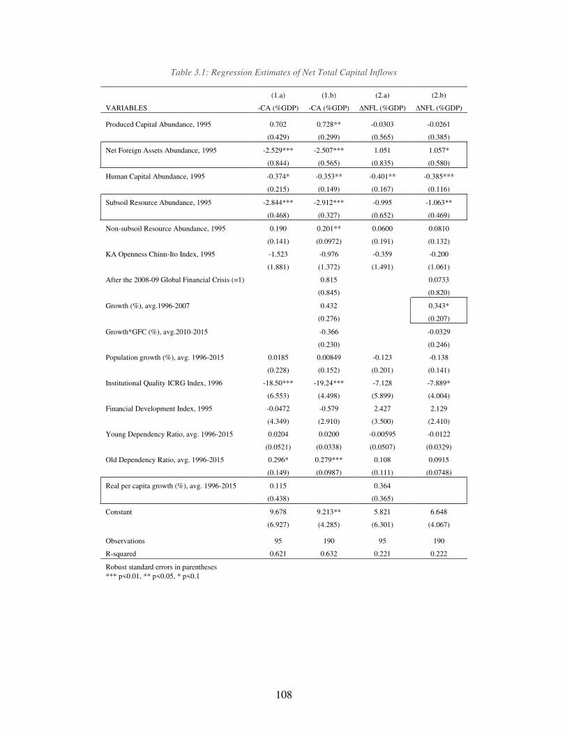
108

Table 3.1: Regression Estimates of Net Total Capital Inflows

(1.a) (1.b) (2.a) (2.b)

VARIABLES -CA (%GDP) -CA (%GDP) ∆NFL (%GDP) ∆NFL (%GDP)

Produced Capital Abundance, 1995 0.702 0.728** -0.0303 -0.0261

(0.429) (0.299) (0.565) (0.385)

Net Foreign Assets Abundance, 1995 -2.529*** -2.507*** 1.051 1.057*

(0.844) (0.565) (0.835) (0.580)

Human Capital Abundance, 1995 -0.374* -0.353** -0.401** -0.385***

(0.215) (0.149) (0.167) (0.116)

Subsoil Resource Abundance, 1995 -2.844*** -2.912*** -0.995 -1.063**

(0.468) (0.327) (0.652) (0.469)

Non-subsoil Resource Abundance, 1995 0.190 0.201** 0.0600 0.0810

(0.141) (0.0972) (0.191) (0.132)

KA Openness Chinn-Ito Index, 1995 -1.523 -0.976 -0.359 -0.200

(1.881) (1.372) (1.491) (1.061)

After the 2008-09 Global Financial Crisis (=1) 0.815 0.0733

(0.845) (0.820)

Growth (%), avg.1996-2007 0.432 0.343*

(0.276) (0.207)

Growth*GFC (%), avg.2010-2015 -0.366 -0.0329

(0.230) (0.246)

Population growth (%), avg. 1996-2015 0.0185 0.00849 -0.123 -0.138

(0.228) (0.152) (0.201) (0.141)

Institutional Quality ICRG Index, 1996 -18.50*** -19.24*** -7.128 -7.889*

(6.553) (4.498) (5.899) (4.004)

Financial Development Index, 1995 -0.0472 -0.579 2.427 2.129

(4.349) (2.910) (3.500) (2.410)

Young Dependency Ratio, avg. 1996-2015 0.0204 0.0200 -0.00595 -0.0122

(0.0521) (0.0338) (0.0507) (0.0329)

Old Dependency Ratio, avg. 1996-2015 0.296* 0.279*** 0.108 0.0915

(0.149) (0.0987) (0.111) (0.0748)

Real per capita growth (%), avg. 1996-2015 0.115 0.364

(0.438) (0.365)

Constant 9.678 9.213** 5.821 6.648

(6.927) (4.285) (6.301) (4.067)


R-squared 0.621 0.632 0.221 0.222


109

Disaggregated Capital Flows

3.5.1 Private versus Official

The distinction between private and official capital flows is of great importance due to

theoretical and empirical considerations. First, many empirical studies find strong evidence that

only private capital flows are in accordance with the neoclassical prediction of efficient

allocation (Aguiar and Amador 2011; Gourinchas and Jeanne 2013; Alfaro et al. 2014). In

addition, Gourinchas and Jeanne (2013) first explain that the decomposition into private and

public should not invalidate the behavior of net total capital flows from the standard neoclassical

viewpoint because of the Ricardian Equivalence assumption— changes in net public and private

borrowing should offset each other in the long run. However, they emphasize that the Ricardian

Equivalence fails if there are financial frictions such as capital controls that affect private flows

differently from public flows (p. 1504). Consequently, relaxing the assumption of the Ricardian

Equivalence could also allow for the possibility of persistent twin deficits—imbalances in the

government budget and CA. As in equation (3.2), if a country decides to run a budget deficit

while individuals do not exactly offset that, the countries must borrow from abroad as captured

by a CA deficit. While the lending countries would associate with CA surpluses or net national

saving. Furthermore, in a recent study, Lowe et al. (2019) distinguish between the public and

private marginal product of capital (MPK) for two reasons. One is that relatively larger

investments in developing countries are public, and the other stems from the literature on

idiosyncratic behavior between public and private agents. The latter includes explanations not

only about efficiency but also redistributive, rent capture, and other policies (p. 337). Finally, the

hegemony of the US dollar in the current international monetary and financial system has also

allowed the US to recycling CA surpluses of some countries to other CA deficit countries and so

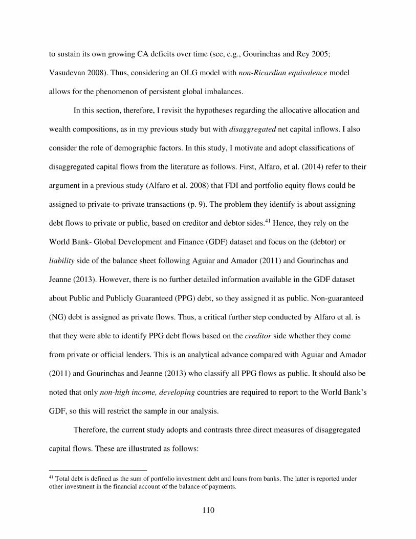
110

to sustain its own growing CA deficits over time (see, e.g., Gourinchas and Rey 2005;

Vasudevan 2008). Thus, considering an OLG model with non-Ricardian equivalence model

allows for the phenomenon of persistent global imbalances.

In this section, therefore, I revisit the hypotheses regarding the allocative allocation and

wealth compositions, as in my previous study but with disaggregated net capital inflows. I also

consider the role of demographic factors. In this study, I motivate and adopt classifications of

disaggregated capital flows from the literature as follows. First, Alfaro, et al. (2014) refer to their

argument in a previous study (Alfaro et al. 2008) that FDI and portfolio equity flows could be

assigned to private-to-private transactions (p. 9). The problem they identify is about assigning

debt flows to private or public, based on creditor and debtor sides.41 Hence, they rely on the

World Bank- Global Development and Finance (GDF) dataset and focus on the (debtor) or

liability side of the balance sheet following Aguiar and Amador (2011) and Gourinchas and

Jeanne (2013). However, there is no further detailed information available in the GDF dataset

about Public and Publicly Guaranteed (PPG) debt, so they assigned it as public. Non-guaranteed

(NG) debt is assigned as private flows. Thus, a critical further step conducted by Alfaro et al. is

that they were able to identify PPG debt flows based on the creditor side whether they come

from private or official lenders. This is an analytical advance compared with Aguiar and Amador

(2011) and Gourinchas and Jeanne (2013) who classify all PPG flows as public. It should also be

noted that only non-high income, developing countries are required to report to the World Bank’s

GDF, so this will restrict the sample in our analysis.

Therefore, the current study adopts and contrasts three direct measures of disaggregated

capital flows. These are illustrated as follows:

41 Total debt is defined as the sum of portfolio investment debt and loans from banks. The latter is reported under other investment in the financial account of the balance of payments.

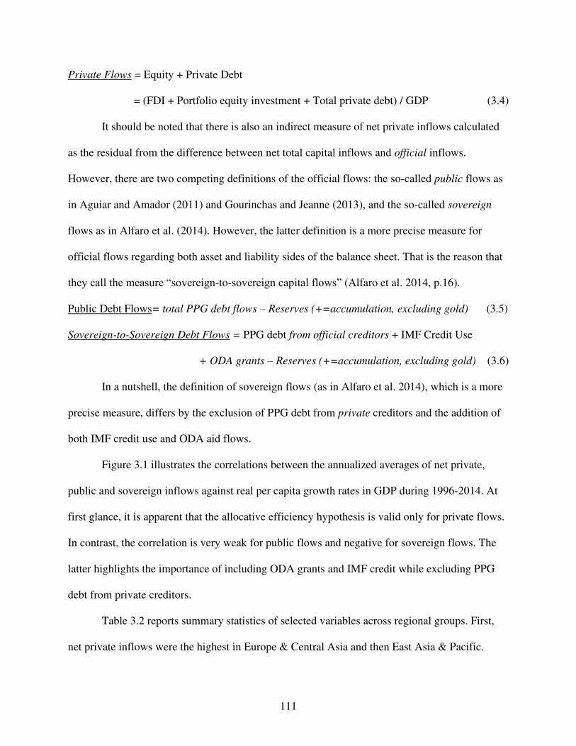
111

Private Flows = Equity + Private Debt

= (FDI + Portfolio equity investment + Total private debt) / GDP (3.4)

It should be noted that there is also an indirect measure of net private inflows calculated

as the residual from the difference between net total capital inflows and official inflows.

However, there are two competing definitions of the official flows: the so-called public flows as

in Aguiar and Amador (2011) and Gourinchas and Jeanne (2013), and the so-called sovereign

flows as in Alfaro et al. (2014). However, the latter definition is a more precise measure for

official flows regarding both asset and liability sides of the balance sheet. That is the reason that

they call the measure “sovereign-to-sovereign capital flows” (Alfaro et al. 2014, p.16).

Public Debt Flows= total PPG debt flows – Reserves (+=accumulation, excluding gold) (3.5)

Sovereign-to-Sovereign Debt Flows = PPG debt from official creditors + IMF Credit Use

+ ODA grants – Reserves (+=accumulation, excluding gold) (3.6)

In a nutshell, the definition of sovereign flows (as in Alfaro et al. 2014), which is a more

precise measure, differs by the exclusion of PPG debt from private creditors and the addition of

both IMF credit use and ODA aid flows.

Figure 3.1 illustrates the correlations between the annualized averages of net private,

public and sovereign inflows against real per capita growth rates in GDP during 1996-2014. At

first glance, it is apparent that the allocative efficiency hypothesis is valid only for private flows.

In contrast, the correlation is very weak for public flows and negative for sovereign flows. The

latter highlights the importance of including ODA grants and IMF credit while excluding PPG

debt from private creditors.

Table 3.2 reports summary statistics of selected variables across regional groups. First,

net private inflows were the highest in Europe & Central Asia and then East Asia & Pacific.

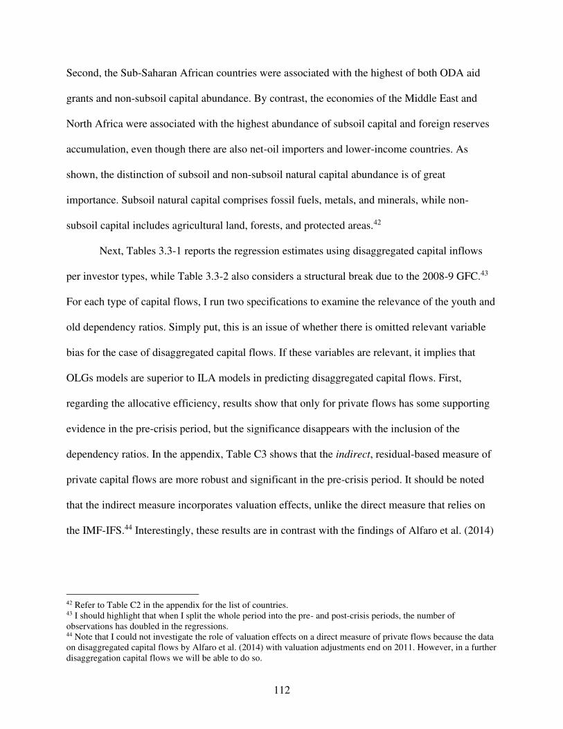
112

Second, the Sub-Saharan African countries were associated with the highest of both ODA aid

grants and non-subsoil capital abundance. By contrast, the economies of the Middle East and

North Africa were associated with the highest abundance of subsoil capital and foreign reserves

accumulation, even though there are also net-oil importers and lower-income countries. As

shown, the distinction of subsoil and non-subsoil natural capital abundance is of great

importance. Subsoil natural capital comprises fossil fuels, metals, and minerals, while non-

subsoil capital includes agricultural land, forests, and protected areas.42

Next, Tables 3.3-1 reports the regression estimates using disaggregated capital inflows

per investor types, while Table 3.3-2 also considers a structural break due to the 2008-9 GFC.43

For each type of capital flows, I run two specifications to examine the relevance of the youth and

old dependency ratios. Simply put, this is an issue of whether there is omitted relevant variable

bias for the case of disaggregated capital flows. If these variables are relevant, it implies that

OLGs models are superior to ILA models in predicting disaggregated capital flows. First,

regarding the allocative efficiency, results show that only for private flows has some supporting

evidence in the pre-crisis period, but the significance disappears with the inclusion of the

dependency ratios. In the appendix, Table C3 shows that the indirect, residual-based measure of

private capital flows are more robust and significant in the pre-crisis period. It should be noted

that the indirect measure incorporates valuation effects, unlike the direct measure that relies on

the IMF-IFS.44 Interestingly, these results are in contrast with the findings of Alfaro et al. (2014)

42 Refer to Table C2 in the appendix for the list of countries. 43 I should highlight that when I split the whole period into the pre- and post-crisis periods, the number of observations has doubled in the regressions. 44 Note that I could not investigate the role of valuation effects on a direct measure of private flows because the data on disaggregated capital flows by Alfaro et al. (2014) with valuation adjustments end on 2011. However, in a further disaggregation capital flows we will be able to do so.

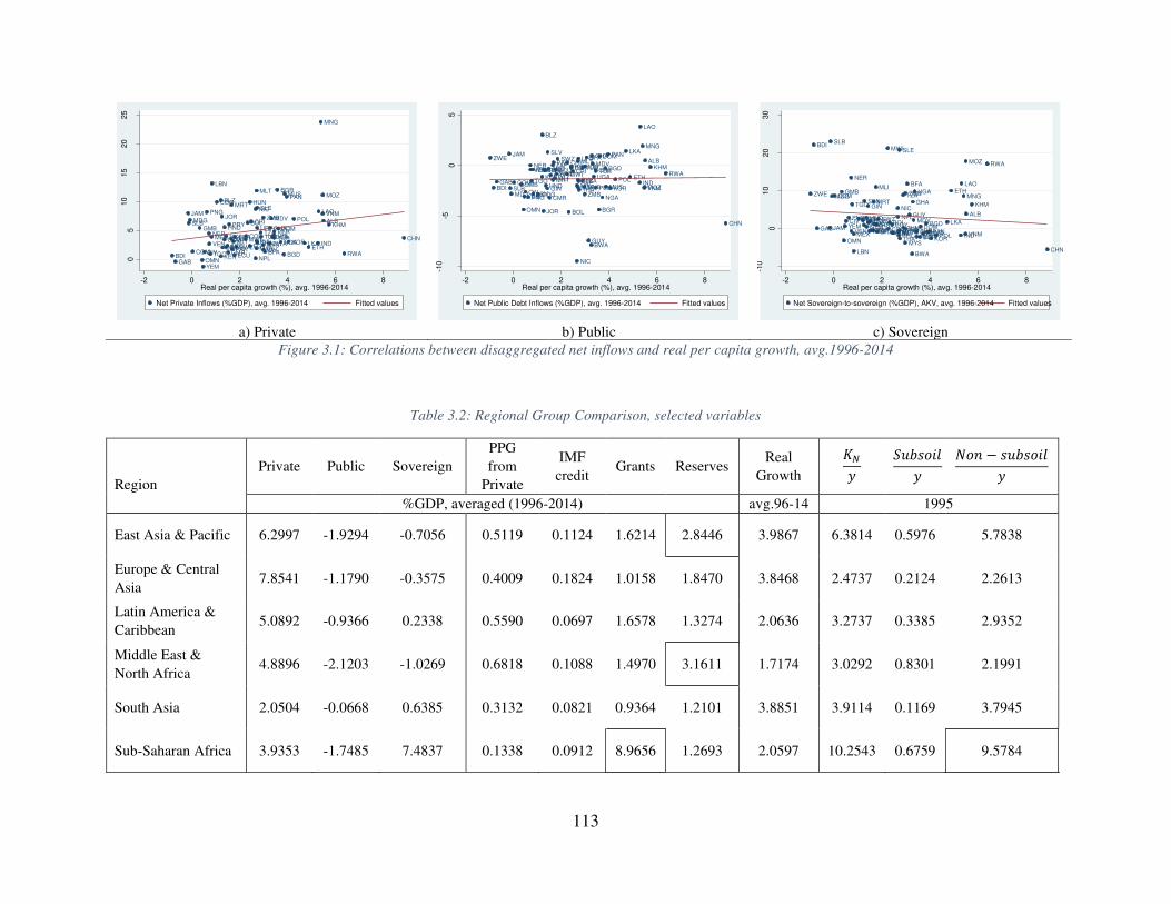
113

Figure 3.1: Correlations between disaggregated net inflows and real per capita growth, avg.1996-2014

Table 3.2: Regional Group Comparison, selected variables

Region

Private Public Sovereign

PPG

from

Private

IMF

credit Grants Reserves

Real

Growth

𝐾𝑁𝑦 𝑆𝑢𝑏𝑠𝑜𝑖𝑙𝑦

𝑁𝑜𝑛 − 𝑠𝑢𝑏𝑠𝑜𝑖𝑙𝑦

%GDP, averaged (1996-2014) avg.96-14 1995

East Asia & Pacific 6.2997 -1.9294 -0.7056 0.5119 0.1124 1.6214 2.8446 3.9867 6.3814 0.5976 5.7838

Europe & Central

Asia 7.8541 -1.1790 -0.3575 0.4009 0.1824 1.0158 1.8470 3.8468 2.4737 0.2124 2.2613

Latin America &

Caribbean 5.0892 -0.9366 0.2338 0.5590 0.0697 1.6578 1.3274 2.0636 3.2737 0.3385 2.9352

Middle East &

North Africa 4.8896 -2.1203 -1.0269 0.6818 0.1088 1.4970 3.1611 1.7174 3.0292 0.8301 2.1991

South Asia 2.0504 -0.0668 0.6385 0.3132 0.0821 0.9364 1.2101 3.8851 3.9114 0.1169 3.7945

Sub-Saharan Africa 3.9353 -1.7485 7.4837 0.1338 0.0912 8.9656 1.2693 2.0597 10.2543 0.6759 9.5784

a) Private

b) Public

c) Sovereign

ALB

ARG

BDIBFA BGD

BGR

BLZ

BOL

BRABWA

CHLCHN

CIV CMR

COG

COL

COM

CRIDOM

ECU

EGY ETH

GAB

GHA

GIN

GMB

GTM

HND

HUN

IDNIND

JAMJOR

KEN

KHM

KOR

LAO

LBN

LKAMAR

MDG MDV

MEXMLI

MLT

MNG

MOZ

MRT

MUS

MWIMYS

NER

NGA

NIC

NPLOMN

PAK

PAN

PER

PHL

PNGPOL

PRY

RWASEN

SLB

SLE

SLV

SWZTGO

THATUN TURTZA

UGA

URY

VEN

VNM

YEM

ZAF

ZMB

05

10

15

20

25

-2 0 2 4 6 8Real per capita growth (%), avg. 1996-2014

Net Private Inflows (%GDP), avg. 1996-2014 Fitted values

ALB

ARG

BDI

BFA

BGD

BGR

BLZ

BOL

BRA

BWA

CHL

CHN

CIVCMR

COG

COL

COM

CRI

DOM

ECU EGY

ETHGAB

GHA

GINGMB

GTM

GUY

HND

HUNIDN

IND

JAM

JOR

KEN

KHM

KOR

LAO

LBN

LKA

MARMDG

MDVMEX

MLI

MLT

MNG

MOZ

MRTMUS

MWI

MYS

NER

NGA

NIC

NPL

OMN

PAK

PAN

PER

PHL

PNG

POLPRY RWA

SEN

SLBSLE

SLVSWZ

TGO

THA

TUNTUR

TZAUGA

URY

VEN

VNM

YEM

ZAF

ZMB

ZWE

-10

-50

5


Net Public Debt Inflows (%GDP), avg. 1996-2014 Fitted values

ALB

ARG

BDI

BFA

BGD

BGR

BLZ BOL

BRA

BWA

CHL

CHN

CIV CMRCOG

COL

COM

CRIDOMECU EGY

ETH

GAB

GHAGIN

GMB

GTM

GUYHND

HUNIDN

IND

JAM JORKEN

KHM

KOR

LAO

LBN

LKA

MAR

MDG

MDV

MEX

MLI

MLT

MNG

MOZ

MRT

MUS

MWI

MYS

NER

NGA

NIC

NPL

OMN

PAK

PANPERPHL

PNG

POLPRY

RWA

SEN

SLB

SLE

SLVSWZ

TGO

THA

TUNTUR

TZAUGA

URYVEN VNM

YEMZAF

ZMBZWE

-10

010

20

30


Net Sovereign-to-sovereign (%GDP), AKV, avg. 1996-2014 Fitted values

114

who concluded that the direct measure of private flows is strongly significant and robust while

the indirect residual-based measures are “very fragile” (p. 24). This could be attributed to either

the sample period or the inclusion of the wealth composition variables. In addition, the

institutional quality index enters with an unexpected negative sign, unlike the case of the direct

measure regressions. Nevertheless, institutional quality remains insignificant.

Columns 2 and 3 of Tables 3.3-1 and 3.3-2 show that the measure choice of public versus

sovereign produces stark differences in the regression results. Some major changes are in the

coefficients of the initial abundance measures of net foreign assets, subsoil and non-subsoil

natural capital, and financial system development. First, the precise measure “sovereign-to-

sovereign” flows, as defined by Alfaro et al (2014), seem to be in accordance with the global

imbalances phenomenon, and with the argument that subsoil-abundant countries tend to have net

official capital outflows on average. Also, the demographic dependency ratios are statistically

and economically significant when considering the sovereign-to-sovereign measure rather than

the public measure. More importantly, the findings of sovereign flows are consistent with those

of total capital flows as reported and discussed in the previous section. Furthermore, the degree

of financial system development seems to matter for net sovereign flows. There is a weakly

negative association although not robust when including the dependency ratios.

The economic effects of wealth compositions are also significant for sovereign flows.

Using the estimates of column 3.b of Table 3.3-1, an increase from the 25th to 75th percentiles in

the initial subsoil abundance, ceteris paribus, associates with a decrease of 0.72 percentage

points in the subsequent annualized average of net sovereign flows to GDP on average. By

contrast, the same increase in the initial non-subsoil abundance associates with an increase of

1.39 percentage points in the subsequent annualized average of net sovereign flows to GDP.

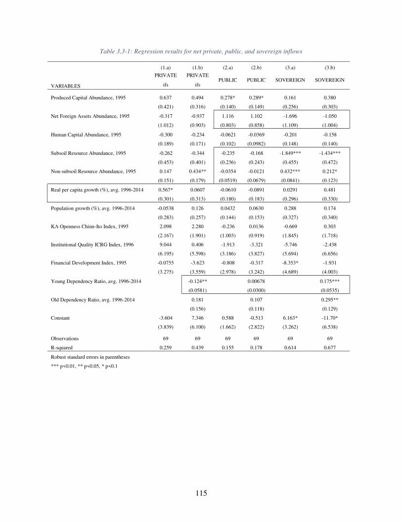
115

Table 3.3-1: Regression results for net private, public, and sovereign inflows

(1.a) (1.b) (2.a) (2.b) (3.a) (3.b)

PRIVATE PRIVATE

PUBLIC PUBLIC SOVEREIGN SOVEREIGN VARIABLES ifs ifs

Produced Capital Abundance, 1995 0.637 0.494 0.278* 0.289* 0.161 0.380

(0.421) (0.316) (0.140) (0.149) (0.256) (0.303)

Net Foreign Assets Abundance, 1995 -0.317 -0.937 1.116 1.102 -1.696 -1.050

(1.012) (0.903) (0.803) (0.858) (1.109) (1.004)

Human Capital Abundance, 1995 -0.300 -0.234 -0.0621 -0.0369 -0.201 -0.158

(0.189) (0.171) (0.102) (0.0982) (0.148) (0.140)

Subsoil Resource Abundance, 1995 -0.262 -0.344 -0.235 -0.168 -1.849*** -1.434***

(0.453) (0.401) (0.236) (0.243) (0.455) (0.472)

Non-subsoil Resource Abundance, 1995 0.147 0.434** -0.0354 -0.0121 0.432*** 0.212*

(0.151) (0.179) (0.0519) (0.0679) (0.0841) (0.123)

Real per capita growth (%), avg. 1996-2014 0.567* 0.0607 -0.0610 -0.0891 0.0291 0.481

(0.301) (0.313) (0.180) (0.183) (0.296) (0.330)

Population growth (%), avg. 1996-2014 -0.0538 0.126 0.0432 0.0630 0.288 0.174

(0.283) (0.257) (0.144) (0.153) (0.327) (0.340)

KA Openness Chinn-Ito Index, 1995 2.098 2.280 -0.236 0.0136 -0.669 0.303

(2.167) (1.901) (1.003) (0.919) (1.845) (1.718)

Institutional Quality ICRG Index, 1996 9.044 0.406 -1.913 -3.321 -5.746 -2.438

(6.195) (5.598) (3.186) (3.827) (5.694) (6.656)

Financial Development Index, 1995 -0.0755 -3.623 -0.808 -0.317 -8.353* -1.931

(3.275) (3.559) (2.978) (3.242) (4.689) (4.003)

Young Dependency Ratio, avg. 1996-2014 -0.124** 0.00678 0.175***

(0.0581) (0.0300) (0.0535)

Old Dependency Ratio, avg. 1996-2014 0.181 0.107 0.295**

(0.156) (0.118) (0.129)

Constant -3.604 7.346 0.588 -0.513 6.163* -11.70*

(3.839) (6.100) (1.662) (2.822) (3.262) (6.538)


R-squared 0.259 0.439 0.155 0.178 0.614 0.677


*** p<0.01, ** p<0.05, * p<0.1

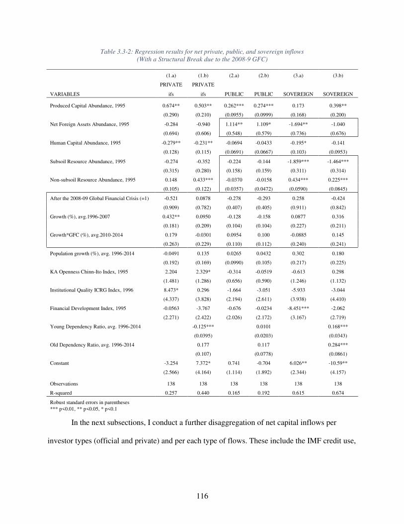
116

Table 3.3-2: Regression results for net private, public, and sovereign inflows

(With a Structural Break due to the 2008-9 GFC)

(1.a) (1.b) (2.a) (2.b) (3.a) (3.b)

PRIVATE PRIVATE

PUBLIC PUBLIC SOVEREIGN SOVEREIGN VARIABLES ifs ifs

Produced Capital Abundance, 1995 0.674** 0.503** 0.262*** 0.274*** 0.173 0.398**

(0.290) (0.210) (0.0955) (0.0999) (0.168) (0.200)

Net Foreign Assets Abundance, 1995 -0.284 -0.940 1.114** 1.109* -1.694** -1.040

(0.694) (0.606) (0.548) (0.579) (0.736) (0.676)

Human Capital Abundance, 1995 -0.279** -0.231** -0.0694 -0.0433 -0.195* -0.141

(0.128) (0.115) (0.0691) (0.0667) (0.103) (0.0953)

Subsoil Resource Abundance, 1995 -0.274 -0.352 -0.224 -0.144 -1.859*** -1.464***

(0.315) (0.280) (0.158) (0.159) (0.311) (0.314)

Non-subsoil Resource Abundance, 1995 0.148 0.433*** -0.0370 -0.0158 0.434*** 0.225***

(0.105) (0.122) (0.0357) (0.0472) (0.0590) (0.0845)

After the 2008-09 Global Financial Crisis (=1) -0.521 0.0878 -0.278 -0.293 0.258 -0.424

(0.909) (0.782) (0.407) (0.405) (0.911) (0.842)

Growth (%), avg.1996-2007 0.432** 0.0950 -0.128 -0.158 0.0877 0.316

(0.181) (0.209) (0.104) (0.104) (0.227) (0.211)

Growth*GFC (%), avg.2010-2014 0.179 -0.0301 0.0954 0.100 -0.0885 0.145

(0.263) (0.229) (0.110) (0.112) (0.240) (0.241)

Population growth (%), avg. 1996-2014 -0.0491 0.135 0.0265 0.0432 0.302 0.180

(0.192) (0.169) (0.0990) (0.105) (0.217) (0.225)

KA Openness Chinn-Ito Index, 1995 2.204 2.329* -0.314 -0.0519 -0.613 0.298

(1.481) (1.286) (0.656) (0.590) (1.246) (1.132)

Institutional Quality ICRG Index, 1996 8.473* 0.296 -1.664 -3.051 -5.933 -3.044

(4.337) (3.828) (2.194) (2.611) (3.938) (4.410)

Financial Development Index, 1995 -0.0563 -3.767 -0.676 -0.0234 -8.451*** -2.062

(2.271) (2.422) (2.026) (2.172) (3.167) (2.719)

Young Dependency Ratio, avg. 1996-2014 -0.125*** 0.0101 0.168***

(0.0395) (0.0203) (0.0343)

Old Dependency Ratio, avg. 1996-2014 0.177 0.117 0.284***

(0.107) (0.0778) (0.0861)

Constant -3.254 7.372* 0.741 -0.704 6.026** -10.59**

(2.566) (4.164) (1.114) (1.892) (2.344) (4.157)

Observations 138 138 138 138 138 138

R-squared 0.257 0.440 0.165 0.192 0.615 0.674


In the next subsections, I conduct a further disaggregation of net capital inflows per

investor types (official and private) and per each type of flows. These include the IMF credit use,

117

official grants, public and publicly guaranteed debt, foreign reserves, FDI, portfolio equity, and

other debt flows.

3.5.2 The Decomposition of Official Flows

Since there are stark differences between the measure choices of the official (public

versus sovereign) flows, I now attempt to highlight the underlying flow types that drive such

differences. First, columns 1-5 of Tables 3.4-1 and 3.4-2 report the regression estimates for the

disaggregated official flows and their sum that makes the difference between the definitions of

public and sovereign flows. Specifically, I replicate the specification with dependency ratios as

in Tables 3.3-1 and 3.3-2 but for more disaggregated official capital flows. Findings suggest that

the difference in the coefficient on subsoil capital abundance is driven by ODA grants, rather

than IMF credit or PPG debt from private creditors. This is apparent by comparing the estimates

of columns 1-4 to those of column 5, which captures the components that make the difference.

This could be justified by the fact that subsoil abundant countries tend to be associated with

high-income economies while being net official aid donors and less dependent on the use of IMF

credit. Conversely, other developing countries with non-subsoil abundance tend to be net official

aid recipients.

Furthermore, column 6 of Table 3.4-1 and 3.4-2 shows that foreign reserves

accumulation is driven on average by the abundance of subsoil capital, rather than any other type

of capital stock, especially in the pre-crisis period. Moreover, the capital account openness index

enters with a significantly positive effect at the 5% level.

Surprisingly, the regression results for ODA grants are puzzling. On the one hand, the

annualized averages of net ODA inflows associate positively with initial physical capital

abundances although the statistical significance is not robust to regression specifications. This

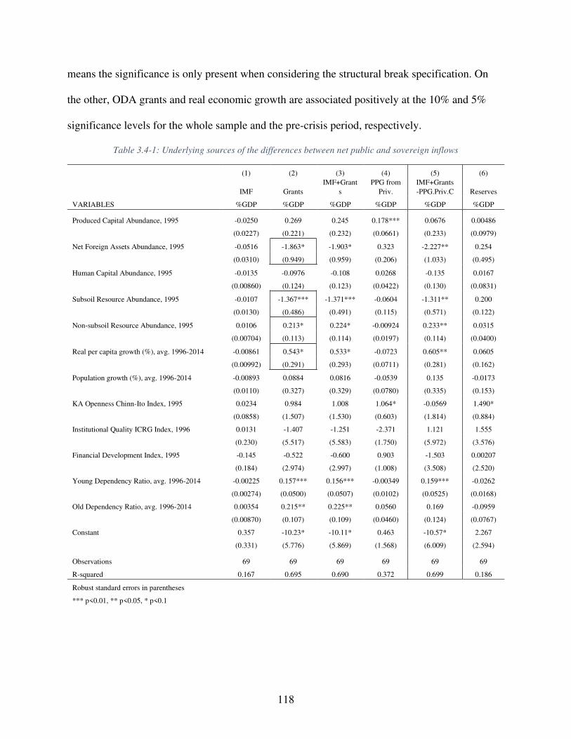
118

means the significance is only present when considering the structural break specification. On

the other, ODA grants and real economic growth are associated positively at the 10% and 5%

significance levels for the whole sample and the pre-crisis period, respectively.

Table 3.4-1: Underlying sources of the differences between net public and sovereign inflows

(1) (2) (3) (4) (5) (6)

IMF Grants

IMF+Grant

s

PPG from

Priv.

IMF+Grants

-PPG.Priv.C Reserves

VARIABLES %GDP %GDP %GDP %GDP %GDP %GDP

Produced Capital Abundance, 1995 -0.0250 0.269 0.245 0.178*** 0.0676 0.00486

(0.0227) (0.221) (0.232) (0.0661) (0.233) (0.0979)

Net Foreign Assets Abundance, 1995 -0.0516 -1.863* -1.903* 0.323 -2.227** 0.254

(0.0310) (0.949) (0.959) (0.206) (1.033) (0.495)

Human Capital Abundance, 1995 -0.0135 -0.0976 -0.108 0.0268 -0.135 0.0167

(0.00860) (0.124) (0.123) (0.0422) (0.130) (0.0831)

Subsoil Resource Abundance, 1995 -0.0107 -1.367*** -1.371*** -0.0604 -1.311** 0.200

(0.0130) (0.486) (0.491) (0.115) (0.571) (0.122)

Non-subsoil Resource Abundance, 1995 0.0106 0.213* 0.224* -0.00924 0.233** 0.0315

(0.00704) (0.113) (0.114) (0.0197) (0.114) (0.0400)

Real per capita growth (%), avg. 1996-2014 -0.00861 0.543* 0.533* -0.0723 0.605** 0.0605

(0.00992) (0.291) (0.293) (0.0711) (0.281) (0.162)

Population growth (%), avg. 1996-2014 -0.00893 0.0884 0.0816 -0.0539 0.135 -0.0173

(0.0110) (0.327) (0.329) (0.0780) (0.335) (0.153)

KA Openness Chinn-Ito Index, 1995 0.0234 0.984 1.008 1.064* -0.0569 1.490*

(0.0858) (1.507) (1.530) (0.603) (1.814) (0.884)

Institutional Quality ICRG Index, 1996 0.0131 -1.407 -1.251 -2.371 1.121 1.555

(0.230) (5.517) (5.583) (1.750) (5.972) (3.576)

Financial Development Index, 1995 -0.145 -0.522 -0.600 0.903 -1.503 0.00207

(0.184) (2.974) (2.997) (1.008) (3.508) (2.520)

Young Dependency Ratio, avg. 1996-2014 -0.00225 0.157*** 0.156*** -0.00349 0.159*** -0.0262

(0.00274) (0.0500) (0.0507) (0.0102) (0.0525) (0.0168)

Old Dependency Ratio, avg. 1996-2014 0.00354 0.215** 0.225** 0.0560 0.169 -0.0959

(0.00870) (0.107) (0.109) (0.0460) (0.124) (0.0767)

Constant 0.357 -10.23* -10.11* 0.463 -10.57* 2.267

(0.331) (5.776) (5.869) (1.568) (6.009) (2.594)


R-squared 0.167 0.695 0.690 0.372 0.699 0.186


*** p<0.01, ** p<0.05, * p<0.1

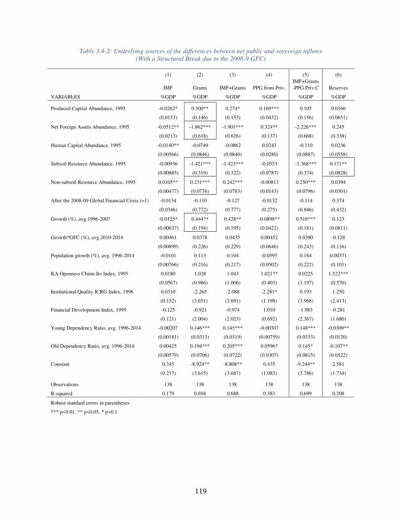
119

Table 3.4-2: Underlying sources of the differences between net public and sovereign inflows


(1) (2) (3) (4) (5) (6)

IMF Grants IMF+Grants PPG from Priv.

IMF+Grants

-PPG.Priv.C Reserves

VARIABLES %GDP %GDP %GDP %GDP %GDP %GDP

Produced Capital Abundance, 1995 -0.0262* 0.300** 0.274* 0.169*** 0.105 0.0166

(0.0153) (0.146) (0.153) (0.0432) (0.156) (0.0651)

Net Foreign Assets Abundance, 1995 -0.0512** -1.862*** -1.901*** 0.324** -2.226*** 0.245

(0.0213) (0.618) (0.626) (0.137) (0.668) (0.338)

Human Capital Abundance, 1995 -0.0140** -0.0749 -0.0862 0.0243 -0.110 0.0236

(0.00566) (0.0846) (0.0840) (0.0280) (0.0887) (0.0558)

Subsoil Resource Abundance, 1995 -0.00936 -1.421*** -1.423*** -0.0553 -1.368*** 0.171**

(0.00885) (0.319) (0.322) (0.0787) (0.374) (0.0828)

Non-subsoil Resource Abundance, 1995 0.0105** 0.231*** 0.242*** -0.00813 0.250*** 0.0394

(0.00477) (0.0776) (0.0783) (0.0143) (0.0796) (0.0301)

After the 2008-09 Global Financial Crisis (=1) -0.0134 -0.110 -0.127 -0.0132 -0.114 0.374

(0.0346) (0.772) (0.777) (0.275) (0.846) (0.432)

Growth (%), avg.1996-2007 -0.0125* 0.444** 0.428** -0.0898** 0.518*** 0.123

(0.00637) (0.194) (0.195) (0.0422) (0.181) (0.0811)

Growth*GFC (%), avg.2010-2014 0.00461 0.0378 0.0435 0.00452 0.0390 -0.128

(0.00899) (0.226) (0.229) (0.0646) (0.243) (0.116)

Population growth (%), avg. 1996-2014 -0.0101 0.113 0.104 -0.0595 0.164 0.00371

(0.00766) (0.216) (0.217) (0.0502) (0.222) (0.101)

KA Openness Chinn-Ito Index, 1995 0.0180 1.028 1.043 1.021** 0.0225 1.522***

(0.0567) (0.986) (1.006) (0.403) (1.197) (0.570)

Institutional Quality ICRG Index, 1996 0.0310 -2.265 -2.088 -2.281* 0.193 1.250

(0.152) (3.651) (3.691) (1.198) (3.968) (2.413)

Financial Development Index, 1995 -0.125 -0.921 -0.974 1.010 -1.983 -0.281

(0.121) (2.004) (2.023) (0.692) (2.367) (1.680)

Young Dependency Ratio, avg. 1996-2014 -0.00207 0.146*** 0.145*** -0.00307 0.148*** -0.0309**

(0.00181) (0.0313) (0.0319) (0.00759) (0.0333) (0.0120)

Old Dependency Ratio, avg. 1996-2014 0.00425 0.194*** 0.205*** 0.0596* 0.145* -0.107**

(0.00579) (0.0706) (0.0722) (0.0307) (0.0815) (0.0522)

Constant 0.345 -8.924** -8.808** 0.435 -9.244** 2.581

(0.217) (3.615) (3.687) (1.083) (3.786) (1.734)

Observations 138 138 138 138 138 138

R-squared 0.179 0.694 0.688 0.383 0.699 0.208


*** p<0.01, ** p<0.05, * p<0.1

120

3.5.3 The Decomposition of Private Flows

After analyzing the disaggregated official capital flows, I now decompose private flows

into FDI, portfolio equity investment, and total private debt. The latter comprises PPG debt flows

from private creditors and non-guaranteed (NG) debt flows in the forms of bank loans, portfolio

debt, and other debt instruments. An important advantage of this further disaggregation is that

the sample size increases due to our lower reliance on the constructed classification of Alfaro et

al. (2014). Moreover, I will investigate the role of valuation effects in the current international

financial system. 45 In contrast to the IMF- International Financial Statistics (IFS), Lane and

Milesi-Ferretti (2017, LM) construct a dataset that incorporates the valuation effects—due to

changes in asset prices and exchange rates—so that capital flows data reflect current market

exchange rates rather than the historical values.

Tables 3.5-1 and 3.5-2 compare the regression estimates for disaggregated net private

equity inflows between the IMF-IFS and Lane and Milesi-Ferretti's datasets. First, it could be

observed that the determinants from our extended theoretical growth framework explain very

little of portfolio flows. Further, they explain relatively little of the observed valuation-adjusted

net FDI inflows. That is, the R-squared value in column 2b is lower than that of 2a.

In addition, overall findings suggest that the allocative efficiency seems to hold only

during the pre-crisis period at best. First, estimates for net total equity inflows, as shown in

columns 3.a and 3.b of Table 3.5-2, validate that during the pre-crisis period at the 5% and 10%

levels, respectively. Regarding FDI flows, the coefficient on real per capita growth rates enters

with opposite signs, indicating the role of valuation effects although results are not strongly

statistically significant nor robust to different specifications. On the other hand, there is positive

45 Although Alfaro et al. (2014) provide data on disaggregated capital flows, data on the valuation-adjusted measure of net total private flows ends in 2011.

121

but insignificant evidence for portfolio equity flows. In sum, while total equity follows, to some

extent, the allocative efficiency during the pre-crisis period, results are inconclusive when I

distinguish between FDI and portfolio equity flows.

Moreover, the estimates indicate the persistence of global imbalances even for net total

private equity flows. Simply put, net creditor countries (NFA>0) in 1995 seem to continue

investing abroad more than foreigners invested in their home countries. While this finding holds

for portfolio and total equity flows, there is an exception for the case of the valuation adjusted

FDI flows, as shown in column 2b.

Regarding the important role of financial system development, the regression results are

interestingly informative. As one could expect that countries that were able to attract higher

portfolio flows during the pre-crisis period, as shown in Table 3.5-2, tend to have highly

developed financial systems. On the contrary, FDI flows are negatively associated with the

degree of financial system development. This could be justified by the characteristics of FDI as

real rather than financial investments.

Further, while both initial abundance measures of subsoil natural capital and human

capital enter negatively, the latter might be puzzling. Also, the statistical significance is present,

as shown in columns 3.a and 3.b of Table 3.5-2, when considering a structural break

specification. Results indicate that countries with a higher abundance of human capital have

associated with net outflows of total equity on average. This could only be justified if we think

about the role of global value chains (GVCs) and that the human capital measure captures the

cost more than the quality of the labor force. On the other hand, subsoil-abundant countries tend

to be classified as high-income economies and to be less attractive for efficiency-seeking foreign

investors.

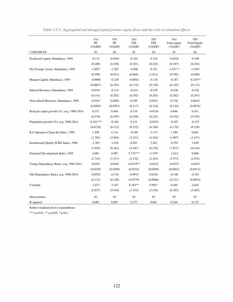
122

Table 3.5-1: Aggregated and disaggregated private equity flows and the role of valuation effects

1(a) 1(b) 2(a) 2(b) 3(a) 3(b)

PE

(%GDP)

PE

(%GDP)

FDI

(%GDP)

FDI

(%GDP)

Total equity

(%GDP)

Total Equity

(%GDP)

VARIABLES ifs lm ifs lm ifs lm

Produced Capital Abundance, 1995 -0.131 -0.0365 0.120 -0.162 -0.0326 -0.199

(0.180) (0.238) (0.181) (0.243) (0.247) (0.242)

Net Foreign Assets Abundance, 1995 -1.001* -1.507 -0.906 0.153 -1.931** -1.354*

(0.598) (0.913) (0.669) (1.011) (0.782) (0.690)

Human Capital Abundance, 1995 -0.0908 -0.129 -0.0916 -0.110 -0.187 -0.238**

(0.0867) (0.103) (0.114) (0.120) (0.145) (0.113)

Subsoil Resource Abundance, 1995 0.0103 -0.114 -0.414 -0.229 -0.436 -0.342

(0.141) (0.202) (0.292) (0.283) (0.282) (0.297)

Non-subsoil Resource Abundance, 1995 0.0163 0.0450 0.109 0.0161 0.138 0.0610

(0.0509) (0.0797) (0.117) (0.124) (0.126) (0.0978)

Real per capita growth (%), avg. 1996-2014 0.351 0.444 0.316 -0.0136 0.646 0.431

(0.370) (0.395) (0.228) (0.225) (0.435) (0.355)

Population growth (%), avg. 1996-2014 -0.243*** -0.104 0.131 -0.0216 -0.107 -0.125

(0.0738) (0.112) (0.152) (0.169) (0.170) (0.120)

KA Openness Chinn-Ito Index, 1995 1.496 4.114 -0.348 -3.313 1.100 0.802

(1.783) (3.892) (2.151) (4.424) (1.997) (1.617)

Institutional Quality ICRG Index, 1996 -1.263 -1.434 0.563 3.262 -0.555 1.828

(7.036) (8.181) (4.187) (6.270) (7.873) (6.414)

Financial Development Index, 1995 4.083 4.987 -5.715*** -4.378* -1.614 0.609

(2.743) (3.317) (2.154) (2.303) (3.573) (2.874)

Young Dependency Ratio, avg. 1996-2014 0.0167 0.0185 -0.0718** -0.0432 -0.0575 -0.0247

(0.0249) (0.0268) (0.0316) (0.0289) (0.0403) (0.0314)

Old Dependency Ratio, avg. 1996-2014 -0.0529 -0.134 -0.0915 0.0326 -0.146 -0.101

(0.113) (0.128) (0.0779) (0.0966) (0.121) (0.0934)

Constant -1.871 -3.447 8.164** 6.091* 6.484 2.644

(5.637) (5.919) (3.353) (3.476) (6.763) (5.492)


R-squared 0.083 0.087 0.277 0.061 0.244 0.135


*** p<0.01, ** p<0.05, * p<0.1

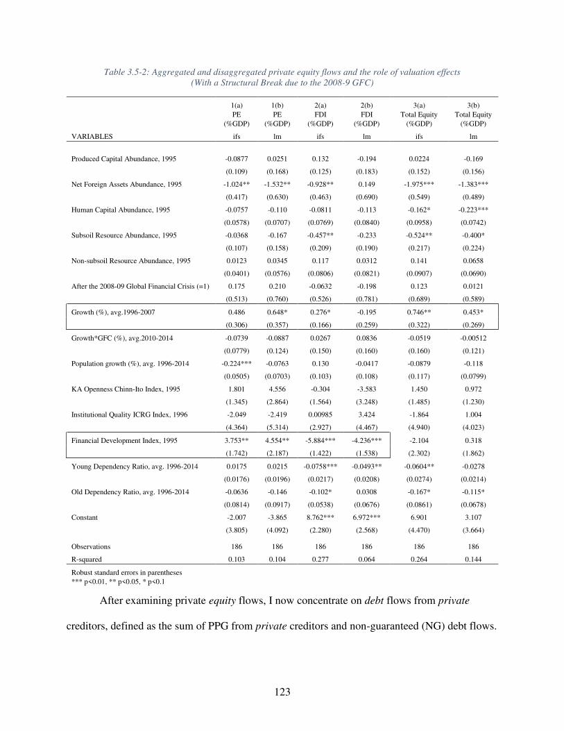
123

Table 3.5-2: Aggregated and disaggregated private equity flows and the role of valuation effects


1(a) 1(b) 2(a) 2(b) 3(a) 3(b)

PE

(%GDP)

PE

(%GDP)

FDI

(%GDP)

FDI

(%GDP)

Total Equity

(%GDP)

Total Equity

(%GDP)

VARIABLES ifs lm ifs lm ifs lm

Produced Capital Abundance, 1995 -0.0877 0.0251 0.132 -0.194 0.0224 -0.169

(0.109) (0.168) (0.125) (0.183) (0.152) (0.156)

Net Foreign Assets Abundance, 1995 -1.024** -1.532** -0.928** 0.149 -1.975*** -1.383***

(0.417) (0.630) (0.463) (0.690) (0.549) (0.489)

Human Capital Abundance, 1995 -0.0757 -0.110 -0.0811 -0.113 -0.162* -0.223***

(0.0578) (0.0707) (0.0769) (0.0840) (0.0958) (0.0742)

Subsoil Resource Abundance, 1995 -0.0368 -0.167 -0.457** -0.233 -0.524** -0.400*

(0.107) (0.158) (0.209) (0.190) (0.217) (0.224)

Non-subsoil Resource Abundance, 1995 0.0123 0.0345 0.117 0.0312 0.141 0.0658

(0.0401) (0.0576) (0.0806) (0.0821) (0.0907) (0.0690)

After the 2008-09 Global Financial Crisis (=1) 0.175 0.210 -0.0632 -0.198 0.123 0.0121

(0.513) (0.760) (0.526) (0.781) (0.689) (0.589)

Growth (%), avg.1996-2007 0.486 0.648* 0.276* -0.195 0.746** 0.453*

(0.306) (0.357) (0.166) (0.259) (0.322) (0.269)

Growth*GFC (%), avg.2010-2014 -0.0739 -0.0887 0.0267 0.0836 -0.0519 -0.00512

(0.0779) (0.124) (0.150) (0.160) (0.160) (0.121)

Population growth (%), avg. 1996-2014 -0.224*** -0.0763 0.130 -0.0417 -0.0879 -0.118

(0.0505) (0.0703) (0.103) (0.108) (0.117) (0.0799)

KA Openness Chinn-Ito Index, 1995 1.801 4.556 -0.304 -3.583 1.450 0.972

(1.345) (2.864) (1.564) (3.248) (1.485) (1.230)

Institutional Quality ICRG Index, 1996 -2.049 -2.419 0.00985 3.424 -1.864 1.004

(4.364) (5.314) (2.927) (4.467) (4.940) (4.023)

Financial Development Index, 1995 3.753** 4.554** -5.884*** -4.236*** -2.104 0.318

(1.742) (2.187) (1.422) (1.538) (2.302) (1.862)

Young Dependency Ratio, avg. 1996-2014 0.0175 0.0215 -0.0758*** -0.0493** -0.0604** -0.0278

(0.0176) (0.0196) (0.0217) (0.0208) (0.0274) (0.0214)

Old Dependency Ratio, avg. 1996-2014 -0.0636 -0.146 -0.102* 0.0308 -0.167* -0.115*

(0.0814) (0.0917) (0.0538) (0.0676) (0.0861) (0.0678)

Constant -2.007 -3.865 8.762*** 6.972*** 6.901 3.107

(3.805) (4.092) (2.280) (2.568) (4.470) (3.664)

Observations 186 186 186 186 186 186

R-squared 0.103 0.104 0.277 0.064 0.264 0.144


After examining private equity flows, I now concentrate on debt flows from private

creditors, defined as the sum of PPG from private creditors and non-guaranteed (NG) debt flows.

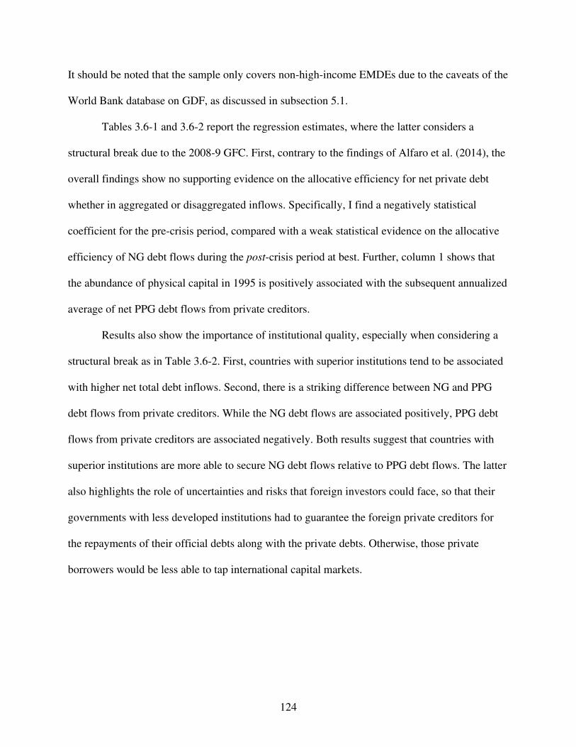
124

It should be noted that the sample only covers non-high-income EMDEs due to the caveats of the

World Bank database on GDF, as discussed in subsection 5.1.

Tables 3.6-1 and 3.6-2 report the regression estimates, where the latter considers a

structural break due to the 2008-9 GFC. First, contrary to the findings of Alfaro et al. (2014), the

overall findings show no supporting evidence on the allocative efficiency for net private debt

whether in aggregated or disaggregated inflows. Specifically, I find a negatively statistical

coefficient for the pre-crisis period, compared with a weak statistical evidence on the allocative

efficiency of NG debt flows during the post-crisis period at best. Further, column 1 shows that

the abundance of physical capital in 1995 is positively associated with the subsequent annualized

average of net PPG debt flows from private creditors.

Results also show the importance of institutional quality, especially when considering a

structural break as in Table 3.6-2. First, countries with superior institutions tend to be associated

with higher net total debt inflows. Second, there is a striking difference between NG and PPG

debt flows from private creditors. While the NG debt flows are associated positively, PPG debt

flows from private creditors are associated negatively. Both results suggest that countries with

superior institutions are more able to secure NG debt flows relative to PPG debt flows. The latter

also highlights the role of uncertainties and risks that foreign investors could face, so that their

governments with less developed institutions had to guarantee the foreign private creditors for

the repayments of their official debts along with the private debts. Otherwise, those private

borrowers would be less able to tap international capital markets.

125

Table 3.6-1: Total and disaggregated debt flows from private creditors

(1) (2) (3)

PPG Debt from

Private Creditors NG Debt

Total Private

Debt

VARIABLES %GDP %GDP %GDP

Produced Capital Abundance, 1995 0.178*** -0.00590 0.172

(0.0666) (0.123) (0.134)

Net Foreign Assets Abundance, 1995 0.312 -0.220 0.0919

(0.209) (0.339) (0.337)

Human Capital Abundance, 1995 0.0226 -0.155** -0.133*

(0.0422) (0.0710) (0.0724)

Subsoil Resource Abundance, 1995 -0.0752 -0.0229 -0.0981

(0.122) (0.186) (0.215)

Non-subsoil Resource Abundance, 1995 -0.00994 0.206** 0.196**

(0.0201) (0.0778) (0.0788)


(0.0748) (0.112) (0.129)

Population growth (%), avg. 1996-2014 -0.0570 0.113 0.0555

(0.0775) (0.104) (0.120)

KA Openness Chinn-Ito Index, 1995 1.075* 0.0849 1.160

(0.597) (0.589) (0.859)

Institutional Quality ICRG Index, 1996 -2.282 5.415*** 3.132

(1.757) (2.026) (2.536)

Financial Development Index, 1995 0.950 -3.102* -2.153

(1.011) (1.674) (1.860)

Young Dependency Ratio, avg. 1996-2014 -0.00304 -0.0693*** -0.0723***

(0.0103) (0.0249) (0.0249)

Old Dependency Ratio, avg. 1996-2014 0.0542 -0.00857 0.0456

(0.0461) (0.0740) (0.0797)

Constant 0.382 2.978 3.360

(1.581) (2.354) (2.590)


R-squared 0.375 0.502 0.510


*** p<0.01, ** p<0.05, * p<0.1

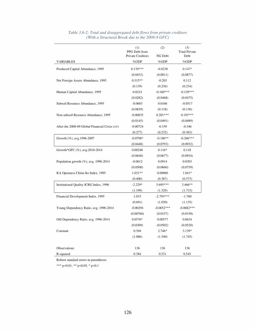
126

Table 3.6-2: Total and disaggregated debt flows from private creditors


(1) (2) (3)

PPG Debt from

Private Creditors NG Debt

Total Private

Debt

VARIABLES %GDP %GDP %GDP

Produced Capital Abundance, 1995 0.170*** -0.0238 0.147*

(0.0432) (0.0811) (0.0877)

Net Foreign Assets Abundance, 1995 0.315** -0.203 0.112

(0.139) (0.236) (0.234)

Human Capital Abundance, 1995 0.0214 -0.160*** -0.139***

(0.0282) (0.0468) (0.0475)

Subsoil Resource Abundance, 1995 -0.0683 0.0166 -0.0517

(0.0839) (0.118) (0.136)

Non-subsoil Resource Abundance, 1995 -0.00835 0.201*** 0.193***

(0.0145) (0.0491) (0.0489)

After the 2008-09 Global Financial Crisis (=1) -0.00724 -0.339 -0.346

(0.277) (0.232) (0.363)

Growth (%), avg.1996-2007 -0.0798* -0.186** -0.266***

(0.0448) (0.0793) (0.0932)

Growth*GFC (%), avg.2010-2014 0.00248 0.116* 0.118

(0.0648) (0.0677) (0.0934)

Population growth (%), avg. 1996-2014 -0.0612 0.0914 0.0303

(0.0500) (0.0660) (0.0759)

KA Openness Chinn-Ito Index, 1995 1.031** 0.00960 1.041*

(0.400) (0.387) (0.573)

Institutional Quality ICRG Index, 1996 -2.229* 5.695*** 3.466**

(1.199) (1.329) (1.715)

Financial Development Index, 1995 1.033 -2.793*** -1.760

(0.691) (1.030) (1.135)

Young Dependency Ratio, avg. 1996-2014 -0.00294 -0.0652*** -0.0682***

(0.00760) (0.0157) (0.0158)

Old Dependency Ratio, avg. 1996-2014 0.0576* 0.00577 0.0634

(0.0309) (0.0502) (0.0520)

Constant 0.394 2.746* 3.139*

(1.086) (1.540) (1.745)


R-squared 0.384 0.531 0.545


*** p<0.01, ** p<0.05, * p<0.1

127


This study utilizes the theoretical insights from OLG models to empirically investigate

the patterns of international capital flows during 1995-2015. Relaxing the strong underlying

assumptions of the Ricardian Equivalence seems to be of great importance in understanding the

saving-investment decisions, and hence, in the external positions. Overall results support the role

of cross-country differences in demographic structures and the distinction of aggregated and

disaggregated capital flows. This implies the superiority of OLG to ILA models, as OLG models

are more general. Thus, findings support the adoption of OLG models with non-Ricardian

equivalence, especially in analyzing capital flows. Moreover, the extended growth framework

with the broad definition of total wealth helps us to better understand the role of economies’

heterogeneities in wealth composition and, hence, in driving aggregated and disaggregated

capital flows. I demonstrate how the heterogeneities in investor types and in countries’ wealth

compositions and demographic structures associate with international capital flows.

Some of the main findings are as follows. First, the inclusion of demographic factors is

found to be relevant and corrects the bias in the estimates. Second, there is, at best, statistical

evidence on the allocative efficiency of total capital flows during the pre-crisis period. Both

results highlight the superiority of OLG to the ILA because of the cross-country difference in

demographic profiles. Further, my previous findings pertain to initial abundance measures of

subsoil capital and NFA positions remain qualitatively unchanged. Also, the disaggregation of

capital flows into private and official shows that only the former validates the allocative

efficiency in the pre-crisis period at best. Moreover, sovereign-to-sovereign flows are found to

be driven by initial abundance measures of subsoil and non-subsoil natural resources. While

Subsoil-abundant countries tended to be associated with net official outflows, non-subsoil-

128

abundant countries tended to be associated with net official inflows. Specifically, subsoil natural

capital seems to be the main determinant of foreign reserve accumulation in the pre-crisis period.

The development of the political and legal institutions, as well as the financial systems,

seem to be critical. First, institutional quality seems to matter most in the decomposition of total

private debt. Countries with superior institutions tend to be more able to borrow abroad without

the need for governments’ guarantees. Regarding equity flows, the degree of financial system

development enters positively in the case of portfolio equity flows, while it enters negatively in

the case of FDI flows. This highlights the characteristics of these flow types, particularly about

financial versus real investment.

Therefore, some policy implications could be drawn based on initial country-specific

conditions and types of capital flows. First, pertaining to net total capital inflows, results show

that subsoil-abundant countries were able to accumulate foreign assets over time. While this

shows, to some extent, that such countries were able to smooth the use of resource windfalls,

they still associate with relatively low averaged growth rates. The former means they have been

considering intergenerational welfare, and the latter highlights the need for other tradable non-

resource sectors, which could induce economy-wide productivity growth. Hence, they should

adopt an industrialization strategy by developing a dynamic comparative advantage, particularly

through the role of economies of scale and scope (see e.g., Vasudevan 2012). Second, since

superior institutional quality allows countries to issue debt liabilities with less need for

government guarantees, so policymakers should improve their legal and political institutions.

129

References

Acemoglu, Daron. 2009. Introduction to Modern Economic Growth. Princeton and Oxford:

Princeton University Press.

Acemoglu, Daron, Simon Johnson, and James A. Robinson. 2001. “The Colonial Origins of

Comparative Development: An Empirical Investigation.” American Economic Review 91

(5): 1369–1401. https://doi.org/10.1257/aer.91.5.1369.

Adler, Gustavo, and Daniel Garcia-Macia. 2018. “The Stabilizing Role of Net Foreign Asset

Returns.” IMF Working Papers 18 (79). https://doi.org/10.5089/9781484349922.001.

Aguiar, Mark, and Manuel Amador. 2011. “Growth in the Shadow of Expropriation.” Quarterly

Journal of Economics 126 (2): 651–97. https://doi.org/10.1093/qje/qjr015.

Aizenman, Joshua, Brian Pinto, and Artur Radziwill. 2007. “Sources for Financing Domestic

Capital - Is Foreign Saving a Viable Option for Developing Countries?” Journal of

International Money and Finance 26 (5): 682–702.

https://doi.org/10.1016/j.jimonfin.2007.04.009.

Alfaro, Laura, Areendam Chanda, Sebnem Kalemli-Ozcan, and Selin Sayek. 2004. “FDI and

Economic Growth: The Role of Local Financial Markets.” Journal of International

Economics 64 (1): 89–112. https://doi.org/10.1016/S0022-1996(03)00081-3.

Alfaro, Laura, Sebnem Kalemli-Ozcan, and Vadym Volosovych. 2008. “Why Doesn’t Capital

Flow from Rich to Poor Countries? An Empirical Investigation.” The Review of Economics

and Statistics 90 (2): 347–68.

130

———. 2014. “Sovereigns, Upstream Capital Flows, and Global Imbalances.” Journal of the

European Economic Association 12 (5): 1240–84. https://doi.org/10.1111/jeea.12106.

Amaglobeli, David, Hua Chai, Era Dabla-norris, Kamil Dybczak, Mauricio Soto, and Alexander

F. Tieman. 2019. “The Future of Saving: The Role of Pension System Design in an Aging

World.” IMF Staff Discussion Note 19/01: 47.

https://www.imf.org/~/media/Files/Publications/SDN/2019/SDN1901.ashx.

Araujo, Juliana D, Antonio C David, Carlos Van Hombeeck, and Chris Papageorgiou. 2015.

“Joining the Club ? Procyclicality of Private Capital Inflows in Low Income Developing

Countries.” IMF Working Paper 70 (163): 157–82.

Balli, Hatice Ozer, and Bent E. Sorensen. 2013. “Interaction Effects in Econometrics.” Empirical

Economics 45 (1): 583–603. https://doi.org/10.1007/s00181-012-0604-2.

Barbier, Edward B. 2007. Natural Resources and Economic Development. Cambridge University

Press.

Barro, Robert J. 1974. “Are Government Bonds Net Wealth?” Journal of Political Economy 82

(6): 1095–1117. https://doi.org/10.1086/260266.

———. 1979. “On the Determination of the Public Debt.” Journal of Political Economy 87 (5,

Part 1): 940–71. https://doi.org/10.1086/260807.

Barro, Robert J., and Jong Wha Lee. 2013. “A New Data Set of Educational Attainment in the

World, 1950-2010.” Journal of Development Economics 104: 184–98.

https://doi.org/10.1016/j.jdeveco.2012.10.001.

Beck, Thorsten. 2011. “Finance and Oil: Is There a Resource Curse in Financial Development?”

131

European Banking Center Discussion Paper 2011–004 (004).

https://doi.org/10.2139/ssrn.1769803.

Bernanke, Ben S. 2005. “The Global Saving Glut and the U.S. Current Account Deficit.”

Remarks at the Virginia Association of Economists.

Blecker, Robert A. 2005. “Financial Globalization, Exchange Rates and International Trade.” In

Financialization and the World Economy, edited by Gerald Epstein, 183–209.

Northampton, MA and Cheltenham, UK: Edward Elgar.

Borensztein, E., J. De Gregorio, and J-W. Lee. 1998. “How Does Foreign Direct Investment

Affect Economic Growth?” Journal of International Economics 45 (1): 115–35.

https://doi.org/10.1016/S0022-1996(97)00033-0.

Boz, Emine, Luis Cubeddu, and Maurice Obstfeld. 2017. “Revisiting the Paradox of Capital.”

VOX CEPR Policy Portal. 2017. https://voxeu.org/article/revisiting-paradox-capital.

Buera, Francisco J, and Yongseok Shin. 2017. “Productivity Growth and Capital Flows :”

American Economic Journal: Macroeconomics 9 (3): 147–85.

Caballero, Ricardo J., Emmanuel Farhi, and Pierre Oliver Gourinchas. 2008. “An Equilibrium

Model of Global Imbalances and Low Interest Rates.” American Economic Review 98 (1):

358–93. https://doi.org/10.1257/aer.98.1.358.

Caballero, Ricardo J., Emmanuel Farhi, and Pierre Olivier Gourinchas. 2017. “The Safe Assets

Shortage Conundrum.” Journal of Economic Perspectives 31 (3): 29–46.

https://doi.org/10.1257/jep.31.3.29.

Calvo, Guillermo A, and Carmen M Reinhart. 2002. “Fear of Floating.” The Quarterly Journal

132

of Economics 117 (2): 379–408.

Carroll, Christopher, Jody Overland, and David Weil. 2000. “Saving and Growth with Habit

Formation.” American Economic Review 90 (3): 341–55.

https://doi.org/10.1257/aer.90.3.341.

Caselli, Francesco, and James Feyrer. 2007. “The Marginal Product of Capital.” The Quarterly

Journal of Economics 122 (2): 535–568.

https://doi.org/https://doi.org/10.1162/qjec.122.2.535.

Chinn, Menzie D, Barry Eichengreen, and Hiro Ito. 2014. “A Forensic Analysis of Global

Imbalances.” Oxford Economic Papers 66 (2): 465–490.

https://doi.org/10.1093/oep/gpt027.

Chinn, Menzie D, and Hiro Ito. 2006. “What Matters for Financial Development? Capital

Controls, Institutions, and Interactions.” Journal of Development Economics 81 (1): 163–

92. https://doi.org/10.1016/j.jdeveco.2005.05.010.

Chinn, Menzie D, and Eswar S Prasad. 2003. “Medium-Term Determinants of Current Accounts

in Industrial and Developing Countries: An Empirical Exploration.” Journal of

International Economics 59: 47–76.

Cooper, Richard N. 2008. “Global Imbalances: Globalization, Demography, and Sustainability.”

Journal of Economic Perspectives 22 (3): 93–112.

Diamond, Peter A. 1965. “National Debt in a Neoclassical Growth Model.” The American

Economic Review 55 (5): 1126–50.

Dooley, Michael, David Folkerts-Landau, and Peter Garber. 2004. “The Revived Bretton Woods

133

System: Alive and Well.” International Journal of Finance and Economics 9 (December):

307–13.

Frankel, Jeffrey. 2012. “The Natural Resource Curse: A Survey of Diagnoses and Some

Prescriptions.” RWP12-014. HKS Faculty Research Working Paper Series.

Frenkel, Roberto, and Lance Taylor. 2006. “Real Exchange Rate, Monetary Policy and

Employment: Economic Development in a Garden of Forking Paths.” Political Economy

Research Institute. Vol. September. Amherst, MA.

Friedman, Milton. 1957. “The Permanent Income Hypothesis.” In A Theory of the Consumption

Function, 20–37. National Bureau of Economic Research.

http://www.nber.org/chapters/c4405.

Gourinchas, Pierre-Olivier, and Olivier Jeanne. 2013. “Capital Flows to Developing Countries :

The Allocation Puzzle.” Review of Economic Studies 80 (4): 1484–1515.

https://doi.org/10.1093/restud/rdt004.

Gourinchas, Pierre-Olivier, and Hélène Rey. 2005. “From World Banker to World Venture

Capitalist: US External Adjustment and the Exorbitant Privilege.” Working Paper No.

11563. Cambridge, MA. http://www.nber.org/papers/w11563.

———. 2015. “External Adjustment, Global Imbalances, Valuation Effects.” In Handbook of

International Economics, edited by Elhanan Helpman, Kenneth Rogoff, and Gita Gopinath,

4:585–645. North Holland: Elsevier B.V. https://doi.org/10.1016/B978-0-444-54314-

1.00010-0.

Gujarati, Damodar, and Dawn Porter. 2009. Basic Econometrics. 5th ed. Boston, Mass:

134

McGraw-Hill.

Gylfason, Thorvaldur. 2004. “Natural Resources and Economic Growth: From Dependence to

Diversification.” CEPR and CESifo.

Hamilton, Kirk, Quentin Wodon, Diego Barrot, and Ali Yedan. 2018. “Human Capital and the

Wealth of Nations: Global Estimates and Trends.” In The Changing Wealth of Nations

2018: Building a Sustainable Future, edited by Glenn-marie Lange, Quentin Wodon, and

Kevin Carey, 115–34. Washington DC: World Bank Group.

Hannan, Swarnali Ahmed. 2017. “The Drivers of Capital Flows in Emerging Markets Post

Global Financial Crisis.” IMF Working Paper WP/17/52 T: 1–26.

Hausmann, Ricardo, Dani Rodrik, and Andrés Velasco. 2005. “Growth Diagnostics.”

http://www.tinyurl.com/y3y5zksu.

International Monetary Fund. 2019a. “External Sector Report: The Dynamics of External

Adjustment.” Washington, DC.

———. 2019b. “Macroeconomic of Aging and Policy Implications.” In Group of 20 - IMF Staff

Note. https://www.imf.org/external/np/g20/pdf/2019/060519a.pdf.

Itskhoki, Oleg, and Dmitry Muhkin. 2019. “Mussa Puzzle Redux.” Working Paper.

http://www.princeton.edu/~itskhoki/papers/Mussa.pdf%0AAbstract.

Kaiser, Henry F., and John Rice. 1974. “Little Jiffy, Mark Iv.” Educational and Psychological

Measurement 34: 111–17. https://doi.org/https://doi.org/10.1177/001316447403400115.

Koepke, Robin. 2015. “What Drives Capital Flows to Emerging Markets ? A Survey of the

Empirical Literature” April 23, (Available at SSRN: https://ssrn.com/abstract=2569249 or

135

http://dx.doi.org/10.2139/ssrn.2569249): 1–45.

Kose, M. Ayhan, Eswar Prasad, Kenneth Rogoff, and Shang Jin Wei. 2010. Financial

Globalization and Economic Policies. Edited by Dani Rodrik and Mark Rosenzweig.

Handbook of Development Economics. 1st ed. Vol. 5. North-Holland: Elsevier B.V.

https://doi.org/10.1016/B978-0-444-52944-2.00003-3.

Krugman, Paul. 1981. “Trade, Accumulation, and Uneven Development.” Journal of

Development Economics 8: 149–61.

Lane, Philip, and Gian Maria Milesi-Ferretti. 2007. “The External Wealth of Nations Mark II:

Revised and Extended Estimates of Foreign Assets and Liabilities, 1970-2004.” Journal of

International Economics 73 (2): 223–50. https://doi.org/10.1016/j.jinteco.2007.02.003.

———. 2017. “International Financial Integration in the Aftermath of the Global Financial

Crisis.” IMF Working Paper 17 (115): 1–53.

Lange, Glenn-marie, Quentin Wodon, and Kevin Carey, eds. 2018. The Changing Wealth of

Nations 2018: Building a Sustainable Future. Washington, DC: World Bank Group.

Lowe, Matt, Chris Papageorgiou, and Fidel Perez-Sebastian. 2019. “The Public and Private

Marginal Product of Capital.” Economica 86 (342): 336–61.

https://doi.org/10.1111/ecca.12268.

Lucas, Robert. 1990. “Why Doesn’t Capital Flow from Rich to Poor Countries?” American

Economic Association 80 (2): 92–96.

Manzano, Osmel, and Roberto Rigobon. 2001. “Resource Curse or Debt Overhang?” Cambridge,

MA. http://www.nber.org/papers/w8390.

136

Mehlum, Halvor, Karl Moene, and Ragnar Torvik. 2006a. “Cursed by Resources or

Institutions ?” The World Economy, 1117–31. https://doi.org/10.1111/j.1467-

9701.2006.00808.x.

———. 2006b. “Institutions and the Resource Curse.” The Economic Journal 116: 1–20.

https://doi.org/10.1111/j.1468-0297.2006.01045.x.

Nakamura, Emi, and Jón Steinsson. 2018. “High-Frequency Identification of Monetary Non-

Neutrality: The Information Effect.” Quarterly Journal of Economics 133 (3): 1283–1330.

https://doi.org/10.1093/QJE/QJY004.

Neumayer, Eric. 2004. “Does the ‘Resource Curse’ Hold for Growth in Genuine Income as

Well ?” 32 (10): 1627–40. https://doi.org/10.1016/j.worlddev.2004.05.005.

Nili, Masoud, and Mahdi Rastad. 2007. “Addressing the Growth Failure of the Oil Economies :

The Role of Financial Development.” The Quarterly Review of Economics and Finance 46:

726–40. https://doi.org/10.1016/j.qref.2006.08.007.

Obstfeld, Maurice. 2017. “Assessing Global Imbalances: The Nuts and Bolts.” IMFBlog:

Insights & Analysis on Economics & Finance, June 26, 2017.

https://blogs.imf.org/2017/06/26/assessing-global-imbalances-the-nuts-and-bolts/.

Obstfeld, Maurice, and Kenneth Rogoff. 1996. Foundations of International Macroeconomics.

Cambridge, Massachusetts: MIT Press.

Palley, Thomas I. 2015. “The Theory of Global Imbalances: Mainstream Economics vs

Structural Keynesianism.” Review of Keynesian Economics 3 (1): 45–62.

https://doi.org/10.4337/roke.2015.01.04.

137

Papaioannou, Elias. 2009. “What Drives International Financial Flows ? Politics, Institutions and

Other Determinants.” Journal of Development Economics 88 (2): 269–81.

https://doi.org/10.1016/j.jdeveco.2008.04.001.

Polterovich, Victor, Vladimir Popov, and Alexander Tonis. 2010. “Resource Abundance: A

Curse or Blessing?” United Nations Working Paper, no. 93.

https://doi.org/10.2139/ssrn.1814382.

Prasad, Eswar, Raghuram Rajan, and Arvind Subramanian. 2007. “Foreign Capital and

Economic Growth.” Brookings Papers on Economic Activity 1: 153–230.

Rajan, Raghuram G, and Arvind Subramanian. 2008. “Aid and Growth: What Does the Cross-

Country Evidence Really Show?” 90 (4): 643–65.

Rodriguez, Francisco, and Jeffrey D. Sachs. 1999. “Why Do Resource-Abundant Economies

Grow More Slowly?” Journal of Economic Growth 4 (3): 277–303.

Rodrik, Dani. 2008. “The Real Exchange Rate and Economic Growth.” Brookings Papers on

Economic Activity 2.

Sachs, Jeffrey, and Andrew Warner. 2001. “The Curse of Natural Resources.” European

Economic Review 45 45: 827–38.

Svirydzenka, Katsiaryna. 2016. “Introducing a New Broad-Based Index of Financial

Development.” IMF Working Paper WP/16/5: 1–43.

Van der Ploeg, Frederick. 2011. “Natural Resources: Curse or Blessing?” Journal of Economic

Literature 49 (2): 366–420. https://doi.org/10.1257/jel.49.2.366.

Van der Ploeg, Frederick, and Steven Poelhekke. 2009. “Volatility and the Natural Resource

138

Curse.” Oxford Economic Papers 61: 727–60. https://doi.org/10.1093/oep/gpp027.

———. 2010. “The Pungent Smell of ‘Red Herrings’: Subsoil Assets, Rents, Volatility and the

Resource Curse.” Journal of Environmental Economics & Management 60 (1): 44–55.

https://doi.org/10.1016/j.jeem.2010.03.003.

Vasudevan, Ramaa. 2008. “The Borrower of Last Resort: International Adjustment and Liquidity

in a Historical Perspective.” Journal of Economic Issues 42 (4): 1055–82.

https://doi.org/10.1080/00213624.2008.11507202.

———. 2009. “Reforming the International Financial System: Core and Periphery Issues and the

Dollar Standard.” EKONOMIAZ. Revista Vasca de Economía 72 (3): 162–79.

———. 2012. “Terms of Trade, Competitive Advantage, and Trade Patterns.” Review of

Political Economy 24 (2): 183–202. https://doi.org/10.1080/09538259.2012.664324.

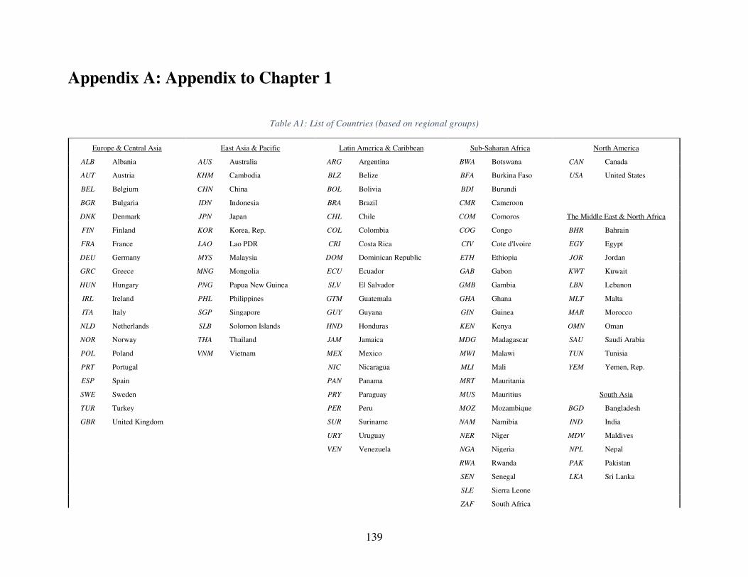
139

Appendix A: Appendix to Chapter 1

Table A1: List of Countries (based on regional groups)

Europe & Central Asia East Asia & Pacific Latin America & Caribbean Sub-Saharan Africa North America

ALB Albania AUS Australia ARG Argentina BWA Botswana CAN Canada

AUT Austria KHM Cambodia BLZ Belize BFA Burkina Faso USA United States

BEL Belgium CHN China BOL Bolivia BDI Burundi

BGR Bulgaria IDN Indonesia BRA Brazil CMR Cameroon

The Middle East & North Africa DNK Denmark JPN Japan CHL Chile COM Comoros

FIN Finland KOR Korea, Rep. COL Colombia COG Congo BHR Bahrain

FRA France LAO Lao PDR CRI Costa Rica CIV Cote d'Ivoire EGY Egypt

DEU Germany MYS Malaysia DOM Dominican Republic ETH Ethiopia JOR Jordan

GRC Greece MNG Mongolia ECU Ecuador GAB Gabon KWT Kuwait

HUN Hungary PNG Papua New Guinea SLV El Salvador GMB Gambia LBN Lebanon

IRL Ireland PHL Philippines GTM Guatemala GHA Ghana MLT Malta

ITA Italy SGP Singapore GUY Guyana GIN Guinea MAR Morocco

NLD Netherlands SLB Solomon Islands HND Honduras KEN Kenya OMN Oman

NOR Norway THA Thailand JAM Jamaica MDG Madagascar SAU Saudi Arabia

POL Poland VNM Vietnam MEX Mexico MWI Malawi TUN Tunisia

PRT Portugal NIC Nicaragua MLI Mali YEM Yemen, Rep.

ESP Spain PAN Panama MRT Mauritania

SWE Sweden PRY Paraguay MUS Mauritius South Asia

TUR Turkey PER Peru MOZ Mozambique BGD Bangladesh

GBR United Kingdom SUR Suriname NAM Namibia IND India

URY Uruguay NER Niger MDV Maldives

VEN Venezuela NGA Nigeria NPL Nepal

RWA Rwanda PAK Pakistan

SEN Senegal LKA Sri Lanka

SLE Sierra Leone

ZAF South Africa

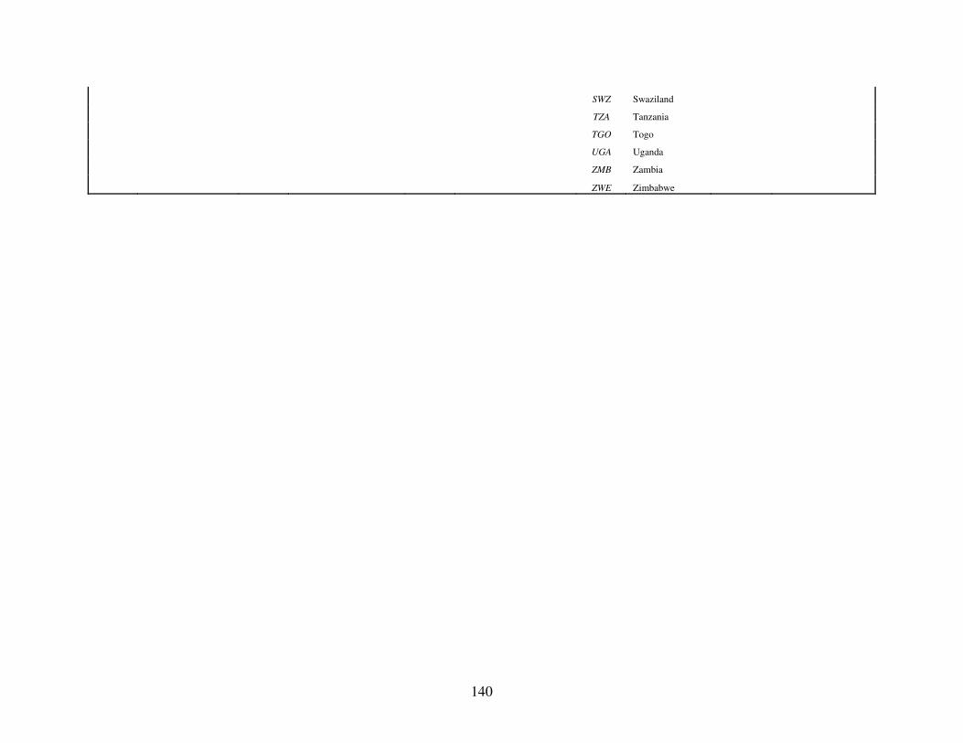
140

SWZ Swaziland

TZA Tanzania

TGO Togo

UGA Uganda

ZMB Zambia

ZWE Zimbabwe

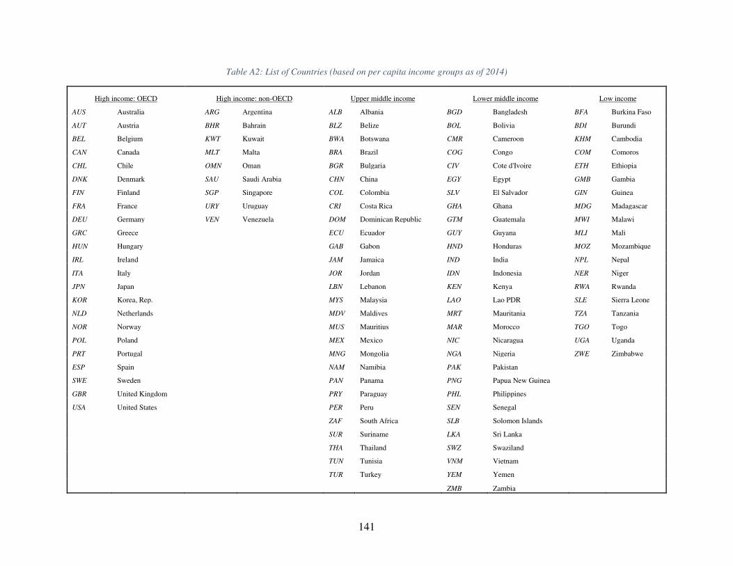
141

Table A2: List of Countries (based on per capita income groups as of 2014)

High income: OECD High income: non-OECD Upper middle income Lower middle income Low income

AUS Australia ARG Argentina ALB Albania BGD Bangladesh BFA Burkina Faso

AUT Austria BHR Bahrain BLZ Belize BOL Bolivia BDI Burundi

BEL Belgium KWT Kuwait BWA Botswana CMR Cameroon KHM Cambodia

CAN Canada MLT Malta BRA Brazil COG Congo COM Comoros

CHL Chile OMN Oman BGR Bulgaria CIV Cote d'Ivoire ETH Ethiopia

DNK Denmark SAU Saudi Arabia CHN China EGY Egypt GMB Gambia

FIN Finland SGP Singapore COL Colombia SLV El Salvador GIN Guinea

FRA France URY Uruguay CRI Costa Rica GHA Ghana MDG Madagascar

DEU Germany VEN Venezuela DOM Dominican Republic GTM Guatemala MWI Malawi

GRC Greece ECU Ecuador GUY Guyana MLI Mali

HUN Hungary GAB Gabon HND Honduras MOZ Mozambique

IRL Ireland JAM Jamaica IND India NPL Nepal

ITA Italy JOR Jordan IDN Indonesia NER Niger

JPN Japan LBN Lebanon KEN Kenya RWA Rwanda

KOR Korea, Rep. MYS Malaysia LAO Lao PDR SLE Sierra Leone

NLD Netherlands MDV Maldives MRT Mauritania TZA Tanzania

NOR Norway MUS Mauritius MAR Morocco TGO Togo

POL Poland MEX Mexico NIC Nicaragua UGA Uganda

PRT Portugal MNG Mongolia NGA Nigeria ZWE Zimbabwe

ESP Spain NAM Namibia PAK Pakistan

SWE Sweden PAN Panama PNG Papua New Guinea

GBR United Kingdom PRY Paraguay PHL Philippines

USA United States PER Peru SEN Senegal

ZAF South Africa SLB Solomon Islands

SUR Suriname LKA Sri Lanka

THA Thailand SWZ Swaziland

TUN Tunisia VNM Vietnam

TUR Turkey YEM Yemen

ZMB Zambia

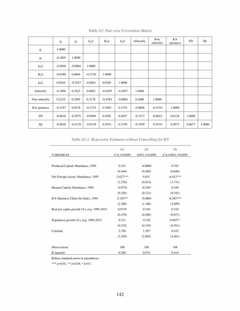
142

Table A3: Pair-wise Correlation Matrix

gy gn kp/y Kf/y kh/y Subsoil/y Non-

subsoil/y KA

openness FD IQ

gy 1.0000

gn -0.1805 1.0000

kp/y -0.0569 -0.0804 1.0000

Kf/y -0.0388 0.0604 -0.2720 1.0000

kh/y 0.0544 -0.2547 -0.0041 0.0305 1.0000

Subsoil/y -0.1896 0.1823 0.0682 -0.0105 -0.2697 1.0000

Non-subsoil/y 0.2219 0.2505 0.3178 -0.4784 -0.0604 0.1000 1.0000

KA openness -0.2397 0.0276 -0.1274 0.3903 0.1535 -0.0686 -0.5310 1.0000

FD -0.0618 -0.3975 -0.0504 0.4501 0.4037 -0.1517 -0.6022 0.6124 1.0000

IQ -0.0820 -0.4178 -0.0139 0.3933 0.3750 -0.1999 -0.5510 0.4972 0.8677 1.0000

Table A5-1: Regression Estimates without Controlling for KN

(1) (2) (3)

VARIABLES -CA (%GDP) ΔNFL (%GDP) -CA+ODA (%GDP)


(0.444) (0.469) (0.640)


(1.278) (0.914) (1.731)

Human Capital Abundance, 1995 -0.0776 -0.236* 0.109

(0.256) (0.121) (0.342)

KA Openness Chinn-Ito Index, 1995 -5.103** -0.0884 -8.285***

(2.289) (1.186) (2.899)


(0.470) (0.266) (0.671)


(0.235) (0.192) (0.361)

Constant 2.356 1.587 0.432

(3.250) (2.085) (4.461)


R-squared 0.289 0.074 0.414


*** p<0.01, ** p<0.05, * p<0.1

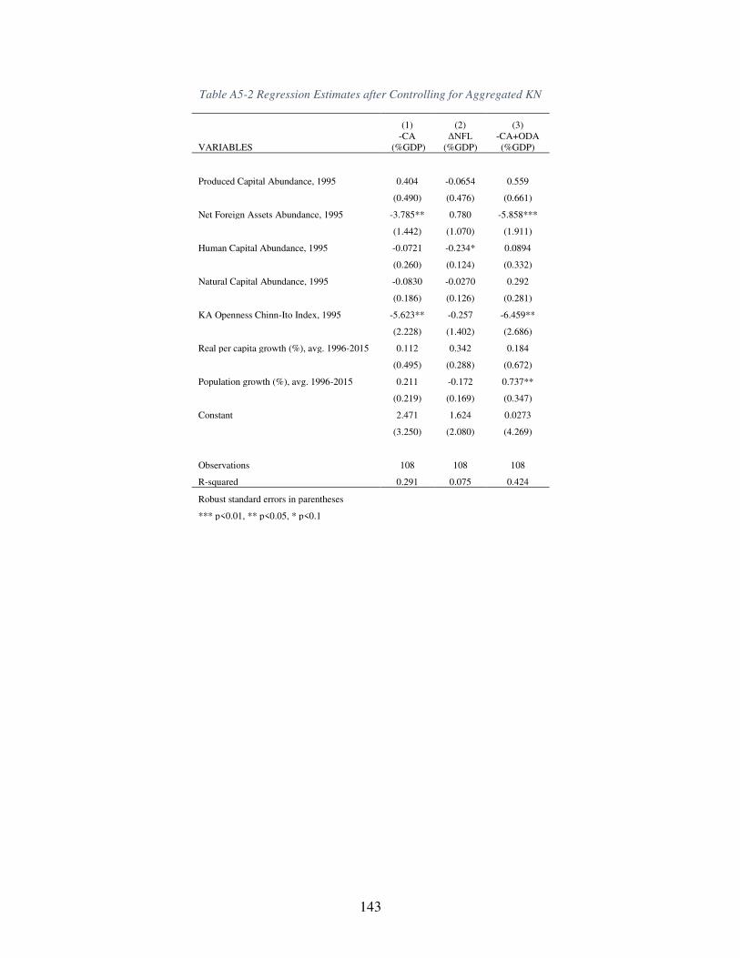
143

Table A5-2 Regression Estimates after Controlling for Aggregated KN

(1) (2) (3)

VARIABLES -CA

(%GDP) ΔNFL



(0.490) (0.476) (0.661)

Net Foreign Assets Abundance, 1995 -3.785** 0.780 -5.858***

(1.442) (1.070) (1.911)

Human Capital Abundance, 1995 -0.0721 -0.234* 0.0894

(0.260) (0.124) (0.332)

Natural Capital Abundance, 1995 -0.0830 -0.0270 0.292

(0.186) (0.126) (0.281)

KA Openness Chinn-Ito Index, 1995 -5.623** -0.257 -6.459**

(2.228) (1.402) (2.686)


(0.495) (0.288) (0.672)


(0.219) (0.169) (0.347)

Constant 2.471 1.624 0.0273

(3.250) (2.080) (4.269)


R-squared 0.291 0.075 0.424


*** p<0.01, ** p<0.05, * p<0.1

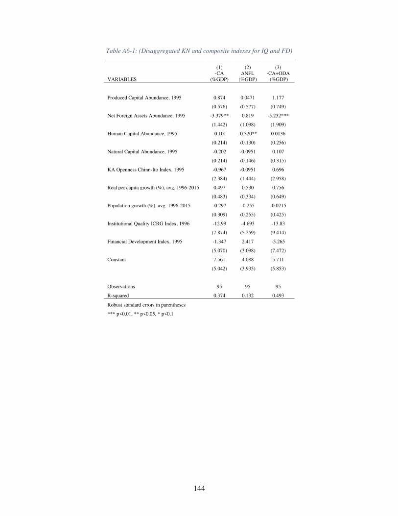
144

Table A6-1: (Disaggregated KN and composite indexes for IQ and FD)

(1) (2) (3)

VARIABLES -CA

(%GDP) ΔNFL


Produced Capital Abundance, 1995 0.874 0.0471 1.177

(0.576) (0.577) (0.749)


(1.442) (1.098) (1.909)

Human Capital Abundance, 1995 -0.101 -0.320** 0.0136

(0.214) (0.130) (0.256)

Natural Capital Abundance, 1995 -0.202 -0.0951 0.107

(0.214) (0.146) (0.315)


(2.384) (1.444) (2.958)


(0.483) (0.334) (0.649)

Population growth (%), avg. 1996-2015 -0.297 -0.255 -0.0215

(0.309) (0.255) (0.425)

Institutional Quality ICRG Index, 1996 -12.99 -4.693 -13.83

(7.874) (5.259) (9.414)

Financial Development Index, 1995 -1.347 2.417 -5.265

(5.070) (3.098) (7.472)

Constant 7.561 4.088 5.711

(5.042) (3.935) (5.853)


R-squared 0.374 0.132 0.493


*** p<0.01, ** p<0.05, * p<0.1

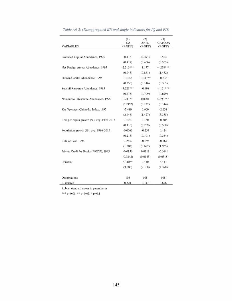
145

Table A6-2: (Disaggregated KN and single indicators for IQ and FD)

(1) (2) (3)

VARIABLES -CA

(%GDP) ΔNFL



(0.417) (0.466) (0.555)


(0.943) (0.861) (1.432)


(0.256) (0.146) (0.305)


(0.473) (0.709) (0.629)


(0.0962) (0.122) (0.144)

KA Openness Chinn-Ito Index, 1995 -2.489 0.600 -2.638

(2.446) (1.427) (3.335)


(0.416) (0.259) (0.568)


(0.213) (0.191) (0.354)

Rule of Law, 1996 -0.964 -0.693 -0.267

(1.302) (0.697) (1.935)

Private Credit by Banks (%GDP), 1995 -0.0156 0.0111 -0.0441

(0.0242) (0.0143) (0.0318)

Constant 6.310** 2.410 6.443

(3.006) (2.108) (4.378)


R-squared 0.524 0.147 0.626


*** p<0.01, ** p<0.05, * p<0.1

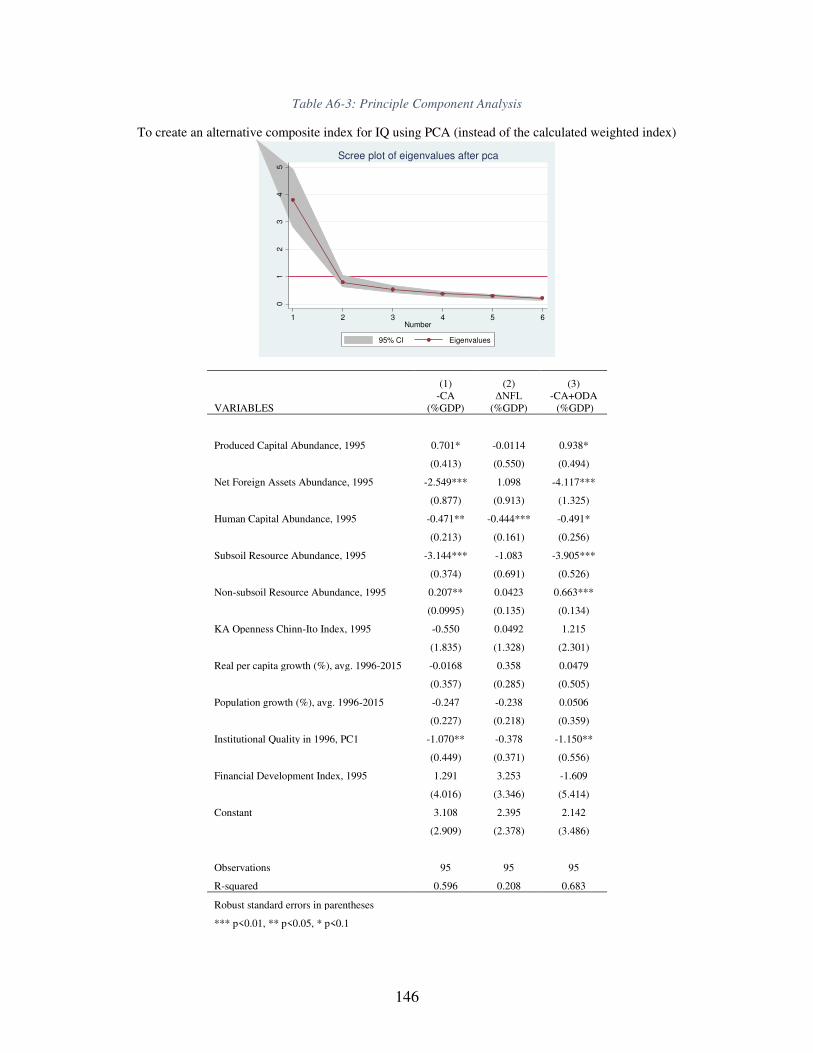
146

Table A6-3: Principle Component Analysis

To create an alternative composite index for IQ using PCA (instead of the calculated weighted index)

(1) (2) (3)

VARIABLES -CA

(%GDP) ΔNFL


Produced Capital Abundance, 1995 0.701* -0.0114 0.938*

(0.413) (0.550) (0.494)


(0.877) (0.913) (1.325)

Human Capital Abundance, 1995 -0.471** -0.444*** -0.491*

(0.213) (0.161) (0.256)


(0.374) (0.691) (0.526)


(0.0995) (0.135) (0.134)

KA Openness Chinn-Ito Index, 1995 -0.550 0.0492 1.215

(1.835) (1.328) (2.301)

Real per capita growth (%), avg. 1996-2015 -0.0168 0.358 0.0479

(0.357) (0.285) (0.505)


(0.227) (0.218) (0.359)

Institutional Quality in 1996, PC1 -1.070** -0.378 -1.150**

(0.449) (0.371) (0.556)

Financial Development Index, 1995 1.291 3.253 -1.609

(4.016) (3.346) (5.414)

Constant 3.108 2.395 2.142

(2.909) (2.378) (3.486)


R-squared 0.596 0.208 0.683


*** p<0.01, ** p<0.05, * p<0.1

01

23

45

1 2 3 4 5 6Number

95% CI Eigenvalues

Scree plot of eigenvalues after pca

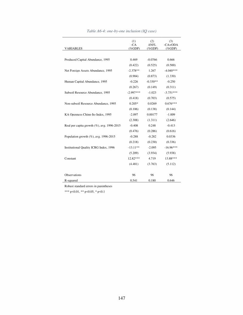
147

Table A6-4: one-by-one inclusion (IQ case)

(1) (2) (3)

VARIABLES -CA

(%GDP) ΔNFL



(0.422) (0.525) (0.500)


(0.904) (0.873) (1.330)


(0.267) (0.149) (0.311)


(0.418) (0.703) (0.575)

Non-subsoil Resource Abundance, 1995 0.205* 0.0269 0.676***

(0.106) (0.138) (0.144)

KA Openness Chinn-Ito Index, 1995 -2.097 0.00177 -1.009

(2.308) (1.311) (2.646)


(0.476) (0.286) (0.616)


(0.218) (0.230) (0.336)

Institutional Quality ICRG Index, 1996 -13.11** -2.095 -16.96***

(5.209) (3.934) (5.938)

Constant 12.82*** 4.719 13.88***

(4.481) (3.763) (5.112)


R-squared 0.541 0.180 0.646


*** p<0.01, ** p<0.05, * p<0.1

148

Table A6-5: one-by-one inclusion (FD case)

(1) (2) (3)

VARIABLES -CA

(%GDP) ΔNFL


Produced Capital Abundance, 1995 0.646 -0.0586 0.852*

(0.391) (0.490) (0.504)


(0.895) (0.899) (1.354)

Human Capital Abundance, 1995 -0.457** -0.444*** -0.339

(0.210) (0.147) (0.278)


(0.445) (0.698) (0.573)


(0.0901) (0.122) (0.135)


(1.877) (1.308) (2.336)


(0.325) (0.250) (0.521)


(0.198) (0.163) (0.331)

Financial Development Index, 1995 -5.954* 2.167 -10.74**

(3.256) (2.459) (4.150)

Constant 6.262** 2.546 5.899

(2.771) (2.218) (3.737)


R-squared 0.572 0.164 0.657


*** p<0.01, ** p<0.05, * p<0.1

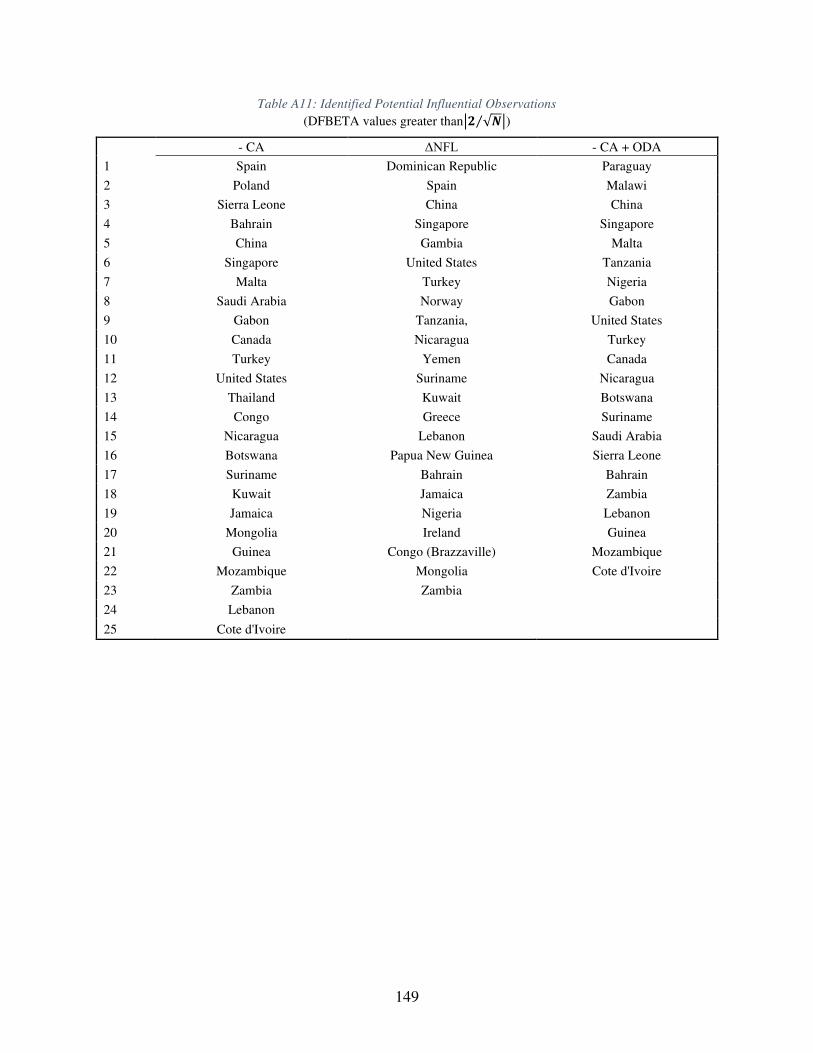
149

Table A11: Identified Potential Influential Observations

(DFBETA values greater than|𝟐 √𝑵⁄ |)

- CA ΔNFL - CA + ODA

1 Spain Dominican Republic Paraguay

2 Poland Spain Malawi

3 Sierra Leone China China

4 Bahrain Singapore Singapore

5 China Gambia Malta

6 Singapore United States Tanzania

7 Malta Turkey Nigeria

8 Saudi Arabia Norway Gabon

9 Gabon Tanzania, United States

10 Canada Nicaragua Turkey

11 Turkey Yemen Canada

12 United States Suriname Nicaragua

13 Thailand Kuwait Botswana

14 Congo Greece Suriname

15 Nicaragua Lebanon Saudi Arabia

16 Botswana Papua New Guinea Sierra Leone

17 Suriname Bahrain Bahrain

18 Kuwait Jamaica Zambia

19 Jamaica Nigeria Lebanon

20 Mongolia Ireland Guinea

21 Guinea Congo (Brazzaville) Mozambique

22 Mozambique Mongolia Cote d'Ivoire

23 Zambia Zambia

24 Lebanon

25 Cote d'Ivoire

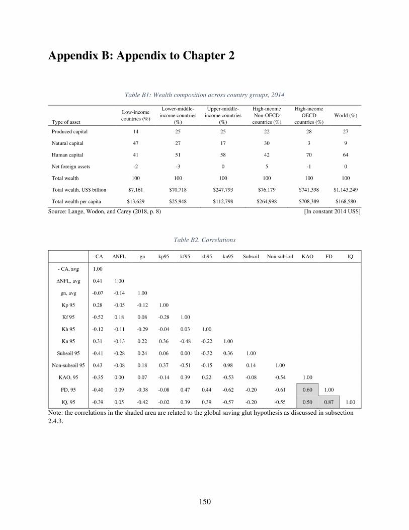
150

Appendix B: Appendix to Chapter 2

Table B1: Wealth composition across country groups, 2014

Type of asset

Low-income

countries (%)

Lower-middle-

income countries

(%)

Upper-middle-

income countries

(%)

High-income

Non-OECD

countries (%)

High-income

OECD

countries (%)

World (%)

Produced capital 14 25 25 22 28 27

Natural capital 47 27 17 30 3 9

Human capital 41 51 58 42 70 64

Net foreign assets -2 -3 0 5 -1 0

Total wealth 100 100 100 100 100 100

Total wealth, US$ billion $7,161 $70,718 $247,793 $76,179 $741,398 $1,143,249

Total wealth per capita $13,629 $25,948 $112,798 $264,998 $708,389 $168,580

Source: Lange, Wodon, and Carey (2018, p. 8) ]In constant 2014 US$ [

Table B2. Correlations

- CA ∆NFL gn kp95 kf95 kh95 kn95 Subsoil Non-subsoil KAO FD IQ

- CA, avg 1.00

∆NFL, avg 0.41 1.00

gn, avg -0.07 -0.14 1.00

Kp 95 0.28 -0.05 -0.12 1.00

Kf 95 -0.52 0.18 0.08 -0.28 1.00

Kh 95 -0.12 -0.11 -0.29 -0.04 0.03 1.00

Kn 95 0.31 -0.13 0.22 0.36 -0.48 -0.22 1.00

Subsoil 95 -0.41 -0.28 0.24 0.06 0.00 -0.32 0.36 1.00

Non-subsoil 95 0.43 -0.08 0.18 0.37 -0.51 -0.15 0.98 0.14 1.00

KAO, 95 -0.35 0.00 0.07 -0.14 0.39 0.22 -0.53 -0.08 -0.54 1.00

FD, 95 -0.40 0.09 -0.38 -0.08 0.47 0.44 -0.62 -0.20 -0.61 0.60 1.00

IQ, 95 -0.39 0.05 -0.42 -0.02 0.39 0.39 -0.57 -0.20 -0.55 0.50 0.87 1.00

Note: the correlations in the shaded area are related to the global saving glut hypothesis as discussed in subsection

2.4.3.

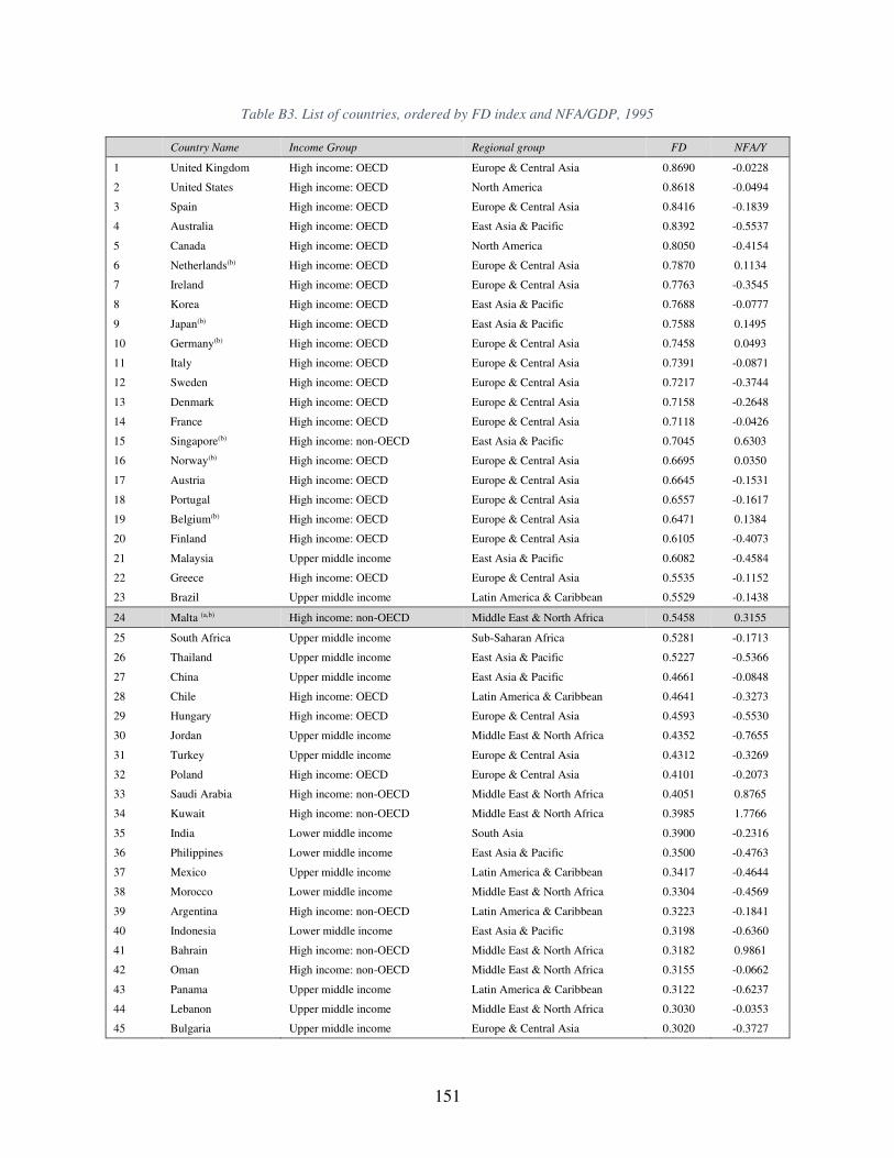
151

Table B3. List of countries, ordered by FD index and NFA/GDP, 1995

Country Name Income Group Regional group FD NFA/Y

1 United Kingdom High income: OECD Europe & Central Asia 0.8690 -0.0228

2 United States High income: OECD North America 0.8618 -0.0494

3 Spain High income: OECD Europe & Central Asia 0.8416 -0.1839

4 Australia High income: OECD East Asia & Pacific 0.8392 -0.5537

5 Canada High income: OECD North America 0.8050 -0.4154

6 Netherlands(b) High income: OECD Europe & Central Asia 0.7870 0.1134

7 Ireland High income: OECD Europe & Central Asia 0.7763 -0.3545

8 Korea High income: OECD East Asia & Pacific 0.7688 -0.0777

9 Japan(b) High income: OECD East Asia & Pacific 0.7588 0.1495

10 Germany(b) High income: OECD Europe & Central Asia 0.7458 0.0493

11 Italy High income: OECD Europe & Central Asia 0.7391 -0.0871

12 Sweden High income: OECD Europe & Central Asia 0.7217 -0.3744

13 Denmark High income: OECD Europe & Central Asia 0.7158 -0.2648

14 France High income: OECD Europe & Central Asia 0.7118 -0.0426

15 Singapore(b) High income: non-OECD East Asia & Pacific 0.7045 0.6303

16 Norway(b) High income: OECD Europe & Central Asia 0.6695 0.0350

17 Austria High income: OECD Europe & Central Asia 0.6645 -0.1531

18 Portugal High income: OECD Europe & Central Asia 0.6557 -0.1617

19 Belgium(b) High income: OECD Europe & Central Asia 0.6471 0.1384

20 Finland High income: OECD Europe & Central Asia 0.6105 -0.4073

21 Malaysia Upper middle income East Asia & Pacific 0.6082 -0.4584

22 Greece High income: OECD Europe & Central Asia 0.5535 -0.1152

23 Brazil Upper middle income Latin America & Caribbean 0.5529 -0.1438

24 Malta (a,b) High income: non-OECD Middle East & North Africa 0.5458 0.3155

25 South Africa Upper middle income Sub-Saharan Africa 0.5281 -0.1713

26 Thailand Upper middle income East Asia & Pacific 0.5227 -0.5366

27 China Upper middle income East Asia & Pacific 0.4661 -0.0848

28 Chile High income: OECD Latin America & Caribbean 0.4641 -0.3273

29 Hungary High income: OECD Europe & Central Asia 0.4593 -0.5530

30 Jordan Upper middle income Middle East & North Africa 0.4352 -0.7655

31 Turkey Upper middle income Europe & Central Asia 0.4312 -0.3269

32 Poland High income: OECD Europe & Central Asia 0.4101 -0.2073

33 Saudi Arabia High income: non-OECD Middle East & North Africa 0.4051 0.8765

34 Kuwait High income: non-OECD Middle East & North Africa 0.3985 1.7766

35 India Lower middle income South Asia 0.3900 -0.2316

36 Philippines Lower middle income East Asia & Pacific 0.3500 -0.4763

37 Mexico Upper middle income Latin America & Caribbean 0.3417 -0.4644

38 Morocco Lower middle income Middle East & North Africa 0.3304 -0.4569

39 Argentina High income: non-OECD Latin America & Caribbean 0.3223 -0.1841

40 Indonesia Lower middle income East Asia & Pacific 0.3198 -0.6360

41 Bahrain High income: non-OECD Middle East & North Africa 0.3182 0.9861

42 Oman High income: non-OECD Middle East & North Africa 0.3155 -0.0662

43 Panama Upper middle income Latin America & Caribbean 0.3122 -0.6237

44 Lebanon Upper middle income Middle East & North Africa 0.3030 -0.0353

45 Bulgaria Upper middle income Europe & Central Asia 0.3020 -0.3727

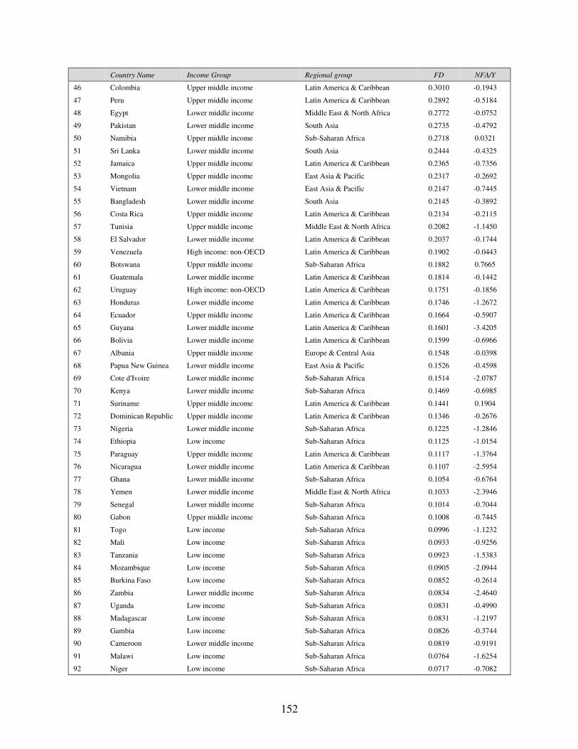
152


46 Colombia Upper middle income Latin America & Caribbean 0.3010 -0.1943

47 Peru Upper middle income Latin America & Caribbean 0.2892 -0.5184

48 Egypt Lower middle income Middle East & North Africa 0.2772 -0.0752

49 Pakistan Lower middle income South Asia 0.2735 -0.4792

50 Namibia Upper middle income Sub-Saharan Africa 0.2718 0.0321

51 Sri Lanka Lower middle income South Asia 0.2444 -0.4325

52 Jamaica Upper middle income Latin America & Caribbean 0.2365 -0.7356

53 Mongolia Upper middle income East Asia & Pacific 0.2317 -0.2692

54 Vietnam Lower middle income East Asia & Pacific 0.2147 -0.7445

55 Bangladesh Lower middle income South Asia 0.2145 -0.3892

56 Costa Rica Upper middle income Latin America & Caribbean 0.2134 -0.2115

57 Tunisia Upper middle income Middle East & North Africa 0.2082 -1.1450

58 El Salvador Lower middle income Latin America & Caribbean 0.2037 -0.1744

59 Venezuela High income: non-OECD Latin America & Caribbean 0.1902 -0.0443

60 Botswana Upper middle income Sub-Saharan Africa 0.1882 0.7665

61 Guatemala Lower middle income Latin America & Caribbean 0.1814 -0.1442

62 Uruguay High income: non-OECD Latin America & Caribbean 0.1751 -0.1856

63 Honduras Lower middle income Latin America & Caribbean 0.1746 -1.2672

64 Ecuador Upper middle income Latin America & Caribbean 0.1664 -0.5907

65 Guyana Lower middle income Latin America & Caribbean 0.1601 -3.4205

66 Bolivia Lower middle income Latin America & Caribbean 0.1599 -0.6966

67 Albania Upper middle income Europe & Central Asia 0.1548 -0.0398

68 Papua New Guinea Lower middle income East Asia & Pacific 0.1526 -0.4598

69 Cote d'Ivoire Lower middle income Sub-Saharan Africa 0.1514 -2.0787

70 Kenya Lower middle income Sub-Saharan Africa 0.1469 -0.6985

71 Suriname Upper middle income Latin America & Caribbean 0.1441 0.1904

72 Dominican Republic Upper middle income Latin America & Caribbean 0.1346 -0.2676

73 Nigeria Lower middle income Sub-Saharan Africa 0.1225 -1.2846

74 Ethiopia Low income Sub-Saharan Africa 0.1125 -1.0154

75 Paraguay Upper middle income Latin America & Caribbean 0.1117 -1.3764

76 Nicaragua Lower middle income Latin America & Caribbean 0.1107 -2.5954

77 Ghana Lower middle income Sub-Saharan Africa 0.1054 -0.6764

78 Yemen Lower middle income Middle East & North Africa 0.1033 -2.3946

79 Senegal Lower middle income Sub-Saharan Africa 0.1014 -0.7044

80 Gabon Upper middle income Sub-Saharan Africa 0.1008 -0.7445

81 Togo Low income Sub-Saharan Africa 0.0996 -1.1232

82 Mali Low income Sub-Saharan Africa 0.0933 -0.9256

83 Tanzania Low income Sub-Saharan Africa 0.0923 -1.5383

84 Mozambique Low income Sub-Saharan Africa 0.0905 -2.0944

85 Burkina Faso Low income Sub-Saharan Africa 0.0852 -0.2614

86 Zambia Lower middle income Sub-Saharan Africa 0.0834 -2.4640

87 Uganda Low income Sub-Saharan Africa 0.0831 -0.4990

88 Madagascar Low income Sub-Saharan Africa 0.0831 -1.2197

89 Gambia Low income Sub-Saharan Africa 0.0826 -0.3744

90 Cameroon Lower middle income Sub-Saharan Africa 0.0819 -0.9191

91 Malawi Low income Sub-Saharan Africa 0.0764 -1.6254

92 Niger Low income Sub-Saharan Africa 0.0717 -0.7082

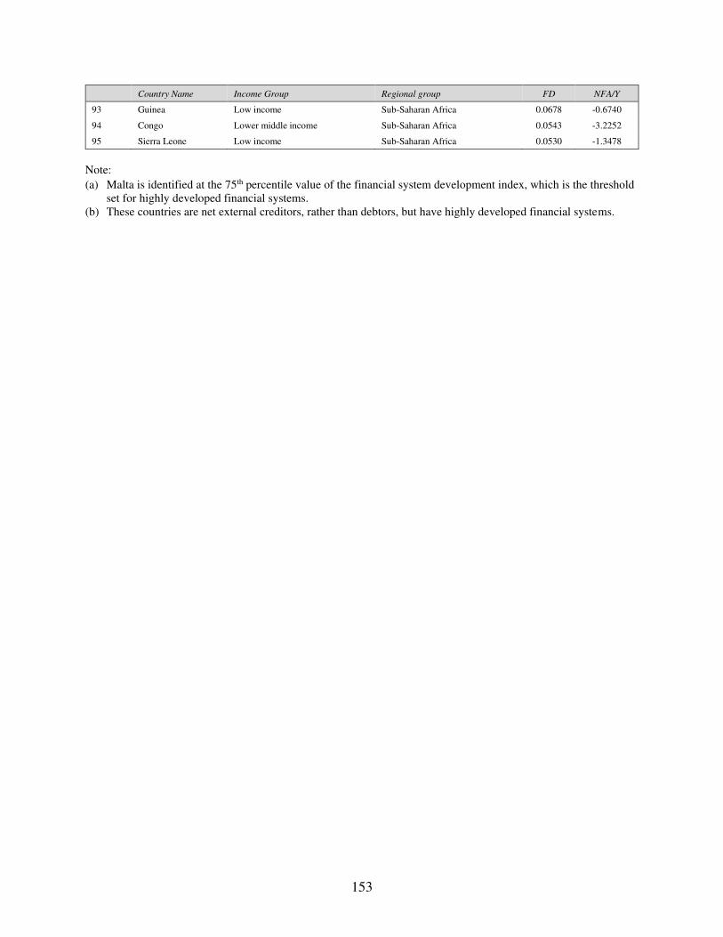
153


93 Guinea Low income Sub-Saharan Africa 0.0678 -0.6740

94 Congo Lower middle income Sub-Saharan Africa 0.0543 -3.2252

95 Sierra Leone Low income Sub-Saharan Africa 0.0530 -1.3478

Note:

(a) Malta is identified at the 75th percentile value of the financial system development index, which is the threshold set for highly developed financial systems.

(b) These countries are net external creditors, rather than debtors, but have highly developed financial systems.

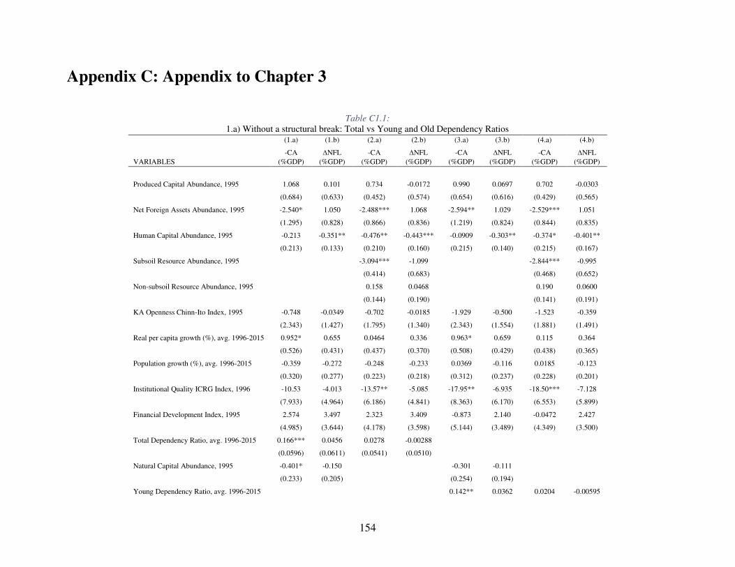
154

Appendix C: Appendix to Chapter 3

Table C1.1:

1.a) Without a structural break: Total vs Young and Old Dependency Ratios

(1.a) (1.b) (2.a) (2.b) (3.a) (3.b) (4.a) (4.b)

VARIABLES

-CA

(%GDP)

∆NFL

(%GDP)

-CA

(%GDP)

∆NFL

(%GDP)

-CA

(%GDP)

∆NFL

(%GDP)

-CA

(%GDP)

∆NFL

(%GDP)

Produced Capital Abundance, 1995 1.068 0.101 0.734 -0.0172 0.990 0.0697 0.702 -0.0303

(0.684) (0.633) (0.452) (0.574) (0.654) (0.616) (0.429) (0.565)

Net Foreign Assets Abundance, 1995 -2.540* 1.050 -2.488*** 1.068 -2.594** 1.029 -2.529*** 1.051

(1.295) (0.828) (0.866) (0.836) (1.219) (0.824) (0.844) (0.835)

Human Capital Abundance, 1995 -0.213 -0.351** -0.476** -0.443*** -0.0909 -0.303** -0.374* -0.401**

(0.213) (0.133) (0.210) (0.160) (0.215) (0.140) (0.215) (0.167)

Subsoil Resource Abundance, 1995 -3.094*** -1.099 -2.844*** -0.995

(0.414) (0.683) (0.468) (0.652)

Non-subsoil Resource Abundance, 1995 0.158 0.0468 0.190 0.0600

(0.144) (0.190) (0.141) (0.191)

KA Openness Chinn-Ito Index, 1995 -0.748 -0.0349 -0.702 -0.0185 -1.929 -0.500 -1.523 -0.359

(2.343) (1.427) (1.795) (1.340) (2.343) (1.554) (1.881) (1.491)

Real per capita growth (%), avg. 1996-2015 0.952* 0.655 0.0464 0.336 0.963* 0.659 0.115 0.364

(0.526) (0.431) (0.437) (0.370) (0.508) (0.429) (0.438) (0.365)

Population growth (%), avg. 1996-2015 -0.359 -0.272 -0.248 -0.233 0.0369 -0.116 0.0185 -0.123

(0.320) (0.277) (0.223) (0.218) (0.312) (0.237) (0.228) (0.201)

Institutional Quality ICRG Index, 1996 -10.53 -4.013 -13.57** -5.085 -17.95** -6.935 -18.50*** -7.128

(7.933) (4.964) (6.186) (4.841) (8.363) (6.170) (6.553) (5.899)

Financial Development Index, 1995 2.574 3.497 2.323 3.409 -0.873 2.140 -0.0472 2.427

(4.985) (3.644) (4.178) (3.598) (5.144) (3.489) (4.349) (3.500)

Total Dependency Ratio, avg. 1996-2015 0.166*** 0.0456 0.0278 -0.00288

(0.0596) (0.0611) (0.0541) (0.0510)

Natural Capital Abundance, 1995 -0.401* -0.150 -0.301 -0.111

(0.233) (0.205) (0.254) (0.194)

Young Dependency Ratio, avg. 1996-2015 0.142** 0.0362 0.0204 -0.00595

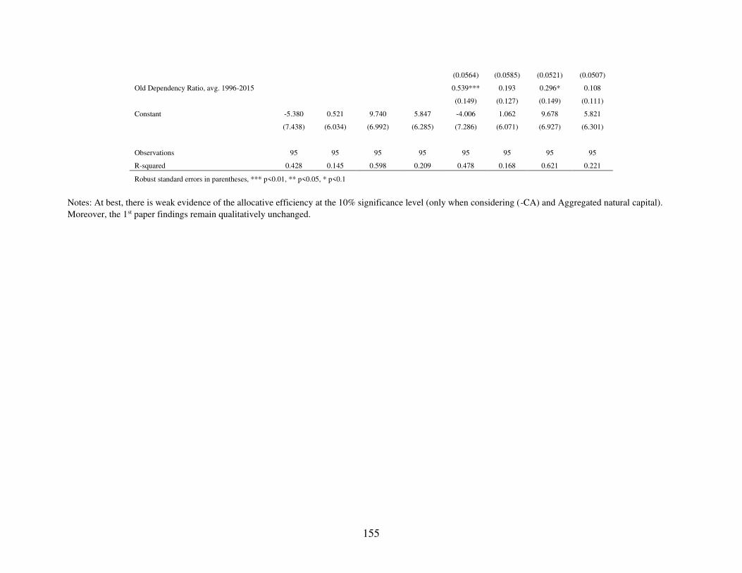
155

(0.0564) (0.0585) (0.0521) (0.0507)

Old Dependency Ratio, avg. 1996-2015 0.539*** 0.193 0.296* 0.108

(0.149) (0.127) (0.149) (0.111)

Constant -5.380 0.521 9.740 5.847 -4.006 1.062 9.678 5.821

(7.438) (6.034) (6.992) (6.285) (7.286) (6.071) (6.927) (6.301)

Observations 95 95 95 95 95 95 95 95

R-squared 0.428 0.145 0.598 0.209 0.478 0.168 0.621 0.221

Robust standard errors in parentheses, *** p<0.01, ** p<0.05, * p<0.1

Notes: At best, there is weak evidence of the allocative efficiency at the 10% significance level (only when considering (-CA) and Aggregated natural capital).

Moreover, the 1st paper findings remain qualitatively unchanged.

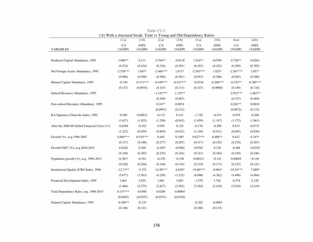
156

Table C1.2:

1.b) With a structural break: Total vs Young and Old Dependency Ratios

(1.a) (1.b) (2.a) (2.b) (3.a) (3.b) (4.a) (4.b)

VARIABLES

-CA

(%GDP)

∆NFL

(%GDP)

-CA

(%GDP)

∆NFL

(%GDP)

-CA

(%GDP)

∆NFL

(%GDP)

-CA

(%GDP)

∆NFL

(%GDP)

Produced Capital Abundance, 1995 1.096** 0.111 0.764** -0.0118 1.014** 0.0789 0.728** -0.0261

(0.474) (0.434) (0.316) (0.391) (0.453) (0.422) (0.299) (0.385)

Net Foreign Assets Abundance, 1995 -2.538*** 1.047* -2.466*** 1.073* -2.593*** 1.025* -2.507*** 1.057*

(0.906) (0.590) (0.580) (0.581) (0.853) (0.586) (0.565) (0.580)

Human Capital Abundance, 1995 -0.149 -0.313*** -0.449*** -0.423*** -0.0336 -0.268*** -0.353** -0.385***

(0.147) (0.0934) (0.147) (0.113) (0.147) (0.0966) (0.149) (0.116)

Subsoil Resource Abundance, 1995 -3.141*** -1.155** -2.912*** -1.063**

(0.290) (0.487) (0.327) (0.469)

Non-subsoil Resource Abundance, 1995 0.167* 0.0674 0.201** 0.0810

(0.0997) (0.132) (0.0972) (0.132)

KA Openness Chinn-Ito Index, 1995 -0.485 0.00815 -0.122 0.142 -1.720 -0.474 -0.976 -0.200

(1.627) (1.025) (1.298) (0.942) (1.659) (1.147) (1.372) (1.061)

After the 2008-09 Global Financial Crisis (=1) -0.0504 -0.242 0.956 0.129 -0.170 -0.289 0.815 0.0733

(1.222) (0.939) (0.859) (0.822) (1.144) (0.921) (0.845) (0.820)

Growth (%), avg.1996-2007 0.884*** 0.510*** 0.445 0.348* 0.827*** 0.488** 0.432 0.343*

(0.317) (0.188) (0.277) (0.207) (0.317) (0.192) (0.276) (0.207)

Growth*GFC (%), avg.2010-2015 0.0226 0.109 -0.429* -0.0582 0.0765 0.130 -0.366 -0.0329

(0.349) (0.285) (0.235) (0.244) (0.321) (0.284) (0.230) (0.246)

Population growth (%), avg. 1996-2015 -0.383* -0.291 -0.239 -0.238 -0.00321 -0.143 0.00849 -0.138

(0.228) (0.204) (0.148) (0.154) (0.219) (0.173) (0.152) (0.141)

Institutional Quality ICRG Index, 1996 -12.73** -5.333 -14.58*** -6.020* -19.80*** -8.094* -19.24*** -7.889*

(5.677) (3.563) (4.250) (3.325) (6.006) (4.362) (4.498) (4.004)


(3.466) (2.575) (2.827) (2.492) (3.454) (2.410) (2.910) (2.410)


(0.0405) (0.0397) (0.0351) (0.0330)

Natural Capital Abundance, 1995 -0.380** -0.135 -0.282 -0.0965

(0.166) (0.141) (0.180) (0.133)

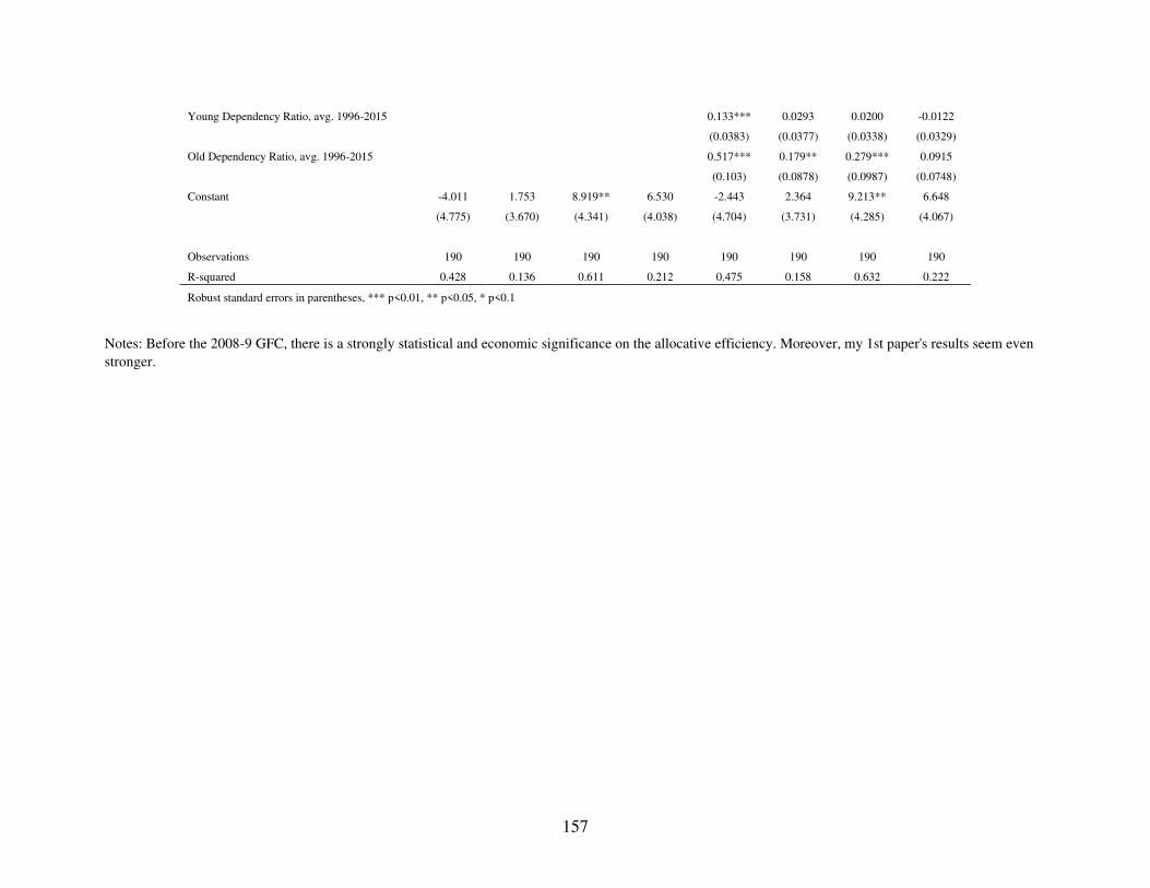
157

Young Dependency Ratio, avg. 1996-2015 0.133*** 0.0293 0.0200 -0.0122

(0.0383) (0.0377) (0.0338) (0.0329)

Old Dependency Ratio, avg. 1996-2015 0.517*** 0.179** 0.279*** 0.0915

(0.103) (0.0878) (0.0987) (0.0748)

Constant -4.011 1.753 8.919** 6.530 -2.443 2.364 9.213** 6.648

(4.775) (3.670) (4.341) (4.038) (4.704) (3.731) (4.285) (4.067)

Observations 190 190 190 190 190 190 190 190

R-squared 0.428 0.136 0.611 0.212 0.475 0.158 0.632 0.222


Notes: Before the 2008-9 GFC, there is a strongly statistical and economic significance on the allocative efficiency. Moreover, my 1st paper's results seem even

stronger.

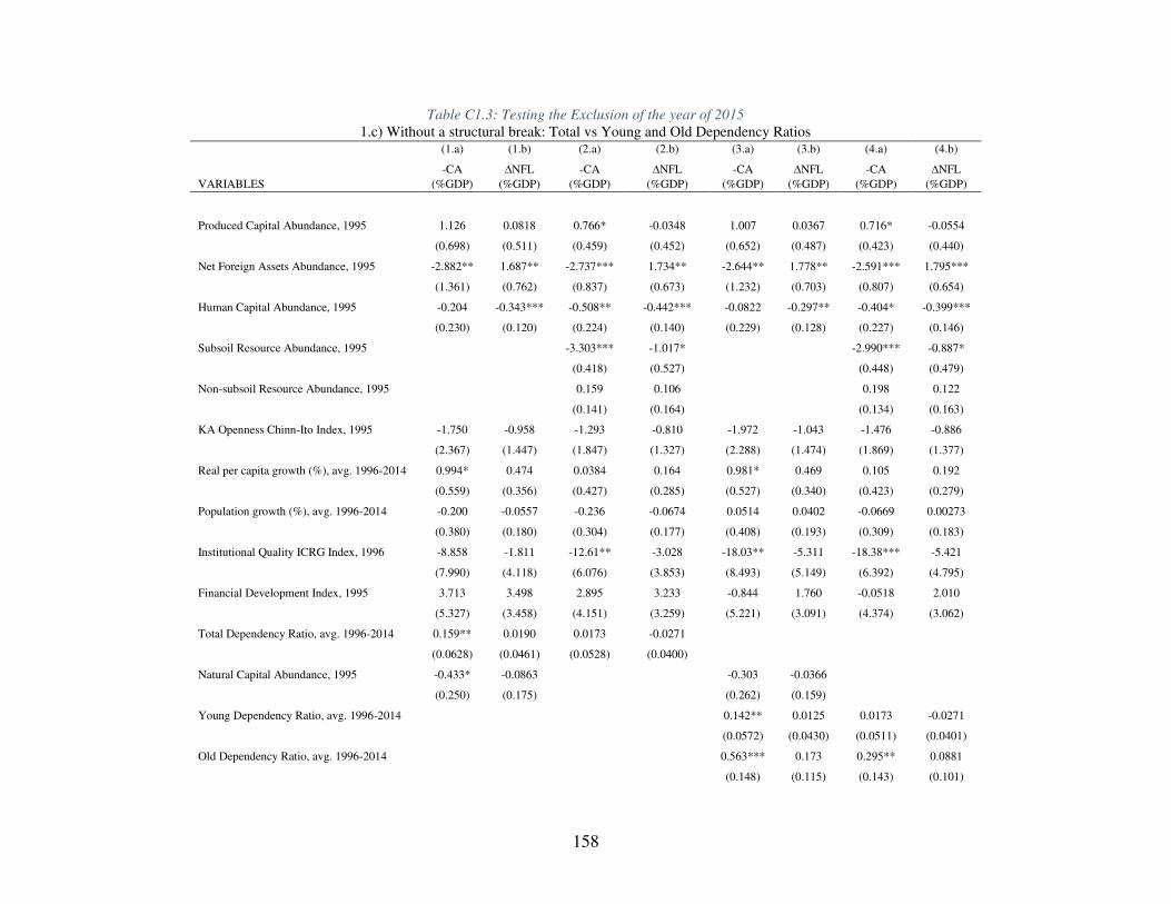
158

Table C1.3: Testing the Exclusion of the year of 2015

1.c) Without a structural break: Total vs Young and Old Dependency Ratios

(1.a) (1.b) (2.a) (2.b) (3.a) (3.b) (4.a) (4.b)

VARIABLES

-CA

(%GDP)

∆NFL

(%GDP)

-CA

(%GDP)

∆NFL

(%GDP)

-CA

(%GDP)

∆NFL

(%GDP)

-CA

(%GDP)

∆NFL

(%GDP)

Produced Capital Abundance, 1995 1.126 0.0818 0.766* -0.0348 1.007 0.0367 0.716* -0.0554

(0.698) (0.511) (0.459) (0.452) (0.652) (0.487) (0.423) (0.440)

Net Foreign Assets Abundance, 1995 -2.882** 1.687** -2.737*** 1.734** -2.644** 1.778** -2.591*** 1.795***

(1.361) (0.762) (0.837) (0.673) (1.232) (0.703) (0.807) (0.654)

Human Capital Abundance, 1995 -0.204 -0.343*** -0.508** -0.442*** -0.0822 -0.297** -0.404* -0.399***

(0.230) (0.120) (0.224) (0.140) (0.229) (0.128) (0.227) (0.146)

Subsoil Resource Abundance, 1995 -3.303*** -1.017* -2.990*** -0.887*

(0.418) (0.527) (0.448) (0.479)

Non-subsoil Resource Abundance, 1995 0.159 0.106 0.198 0.122

(0.141) (0.164) (0.134) (0.163)


(2.367) (1.447) (1.847) (1.327) (2.288) (1.474) (1.869) (1.377)

Real per capita growth (%), avg. 1996-2014 0.994* 0.474 0.0384 0.164 0.981* 0.469 0.105 0.192

(0.559) (0.356) (0.427) (0.285) (0.527) (0.340) (0.423) (0.279)

Population growth (%), avg. 1996-2014 -0.200 -0.0557 -0.236 -0.0674 0.0514 0.0402 -0.0669 0.00273

(0.380) (0.180) (0.304) (0.177) (0.408) (0.193) (0.309) (0.183)

Institutional Quality ICRG Index, 1996 -8.858 -1.811 -12.61** -3.028 -18.03** -5.311 -18.38*** -5.421

(7.990) (4.118) (6.076) (3.853) (8.493) (5.149) (6.392) (4.795)


(5.327) (3.458) (4.151) (3.259) (5.221) (3.091) (4.374) (3.062)

Total Dependency Ratio, avg. 1996-2014 0.159** 0.0190 0.0173 -0.0271

(0.0628) (0.0461) (0.0528) (0.0400)

Natural Capital Abundance, 1995 -0.433* -0.0863 -0.303 -0.0366

(0.250) (0.175) (0.262) (0.159)

Young Dependency Ratio, avg. 1996-2014 0.142** 0.0125 0.0173 -0.0271

(0.0572) (0.0430) (0.0511) (0.0401)

Old Dependency Ratio, avg. 1996-2014 0.563*** 0.173 0.295** 0.0881

(0.148) (0.115) (0.143) (0.101)

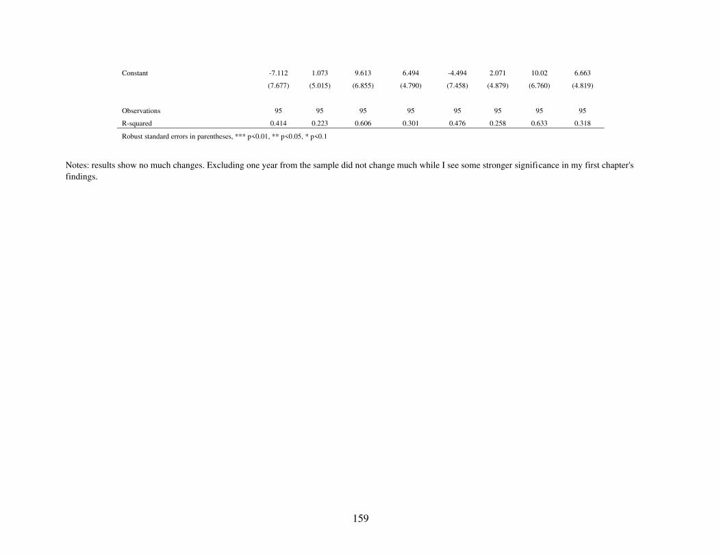
159

Constant -7.112 1.073 9.613 6.494 -4.494 2.071 10.02 6.663

(7.677) (5.015) (6.855) (4.790) (7.458) (4.879) (6.760) (4.819)

Observations 95 95 95 95 95 95 95 95

R-squared 0.414 0.223 0.606 0.301 0.476 0.258 0.633 0.318


Notes: results show no much changes. Excluding one year from the sample did not change much while I see some stronger significance in my first chapter's

findings.

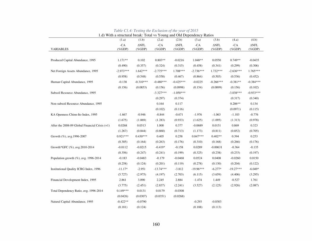
160

Table C1.4: Testing the Exclusion of the year of 2015

1.d) With a structural break: Total vs Young and Old Dependency Ratios

(1.a) (1.b) (2.a) (2.b) (3.a) (3.b) (4.a) (4.b)

VARIABLES

-CA

(%GDP)

∆NFL

(%GDP)

-CA

(%GDP)

∆NFL

(%GDP)

-CA

(%GDP)

∆NFL

(%GDP)

-CA

(%GDP)

∆NFL

(%GDP)

Produced Capital Abundance, 1995 1.171** 0.102 0.803** -0.0216 1.048** 0.0550 0.749** -0.0435

(0.490) (0.357) (0.324) (0.315) (0.458) (0.341) (0.299) (0.306)

Net Foreign Assets Abundance, 1995 -2.973*** 1.642*** -2.775*** 1.708*** -2.736*** 1.732*** -2.636*** 1.765***

(0.958) (0.548) (0.558) (0.467) (0.864) (0.503) (0.536) (0.452)

Human Capital Abundance, 1995 -0.138 -0.310*** -0.480*** -0.425*** -0.0225 -0.266*** -0.381** -0.384***

(0.156) (0.0853) (0.156) (0.0998) (0.154) (0.0899) (0.156) (0.102)

Subsoil Resource Abundance, 1995 -3.327*** -1.050*** -3.038*** -0.933***

(0.297) (0.374) (0.317) (0.340)

Non-subsoil Resource Abundance, 1995 0.164 0.117 0.206** 0.134

(0.102) (0.116) (0.0971) (0.115)


(1.675) (1.069) (1.283) (0.933) (1.625) (1.095) (1.313) (0.978)

After the 2008-09 Global Financial Crisis (=1) 0.0268 0.0513 1.000 0.377 -0.0689 0.0151 0.869 0.323

(1.267) (0.844) (0.860) (0.713) (1.173) (0.811) (0.852) (0.705)

Growth (%), avg.1996-2007 0.921*** 0.430*** 0.405 0.258 0.847*** 0.402** 0.394 0.253

(0.305) (0.164) (0.263) (0.176) (0.310) (0.168) (0.266) (0.176)

Growth*GFC (%), avg.2010-2014 -0.0112 -0.0215 -0.419* -0.158 0.0289 -0.00631 -0.364 -0.135

(0.356) (0.247) (0.241) (0.199) (0.325) (0.238) (0.233) (0.197)

Population growth (%), avg. 1996-2014 -0.183 -0.0483 -0.179 -0.0468 0.0524 0.0408 -0.0260 0.0150

(0.258) (0.124) (0.201) (0.119) (0.278) (0.130) (0.204) (0.122)

Institutional Quality ICRG Index, 1996 -11.17* -2.951 -13.74*** -3.812 -19.96*** -6.277* -19.27*** -6.049*

(5.727) (2.975) (4.197) (2.703) (6.115) (3.659) (4.406) (3.295)


(3.775) (2.451) (2.837) (2.241) (3.527) (2.125) (2.926) (2.087)


(0.0426) (0.0307) (0.0351) (0.0268)

Natural Capital Abundance, 1995 -0.422** -0.0790 -0.293 -0.0303

(0.181) (0.124) (0.188) (0.113)

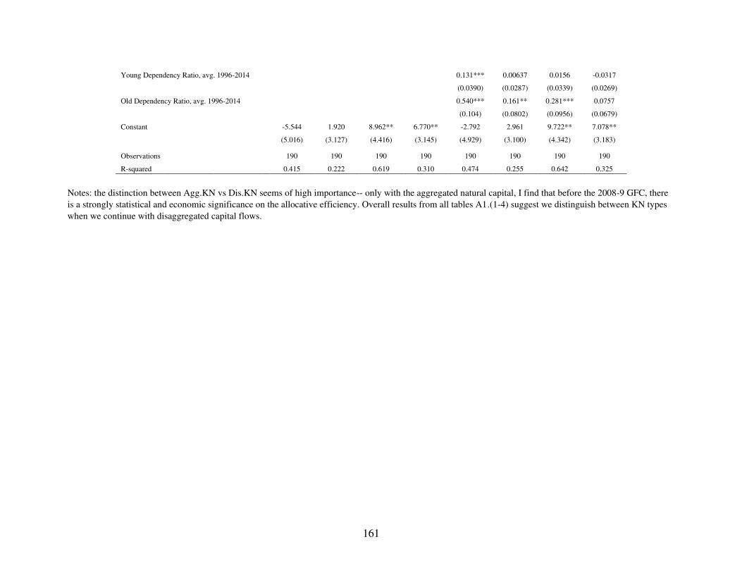
161

Young Dependency Ratio, avg. 1996-2014 0.131*** 0.00637 0.0156 -0.0317

(0.0390) (0.0287) (0.0339) (0.0269)

Old Dependency Ratio, avg. 1996-2014 0.540*** 0.161** 0.281*** 0.0757

(0.104) (0.0802) (0.0956) (0.0679)

Constant -5.544 1.920 8.962** 6.770** -2.792 2.961 9.722** 7.078**

(5.016) (3.127) (4.416) (3.145) (4.929) (3.100) (4.342) (3.183)

Observations 190 190 190 190 190 190 190 190

R-squared 0.415 0.222 0.619 0.310 0.474 0.255 0.642 0.325

Notes: the distinction between Agg.KN vs Dis.KN seems of high importance-- only with the aggregated natural capital, I find that before the 2008-9 GFC, there

is a strongly statistical and economic significance on the allocative efficiency. Overall results from all tables A1.(1-4) suggest we distinguish between KN types

when we continue with disaggregated capital flows.

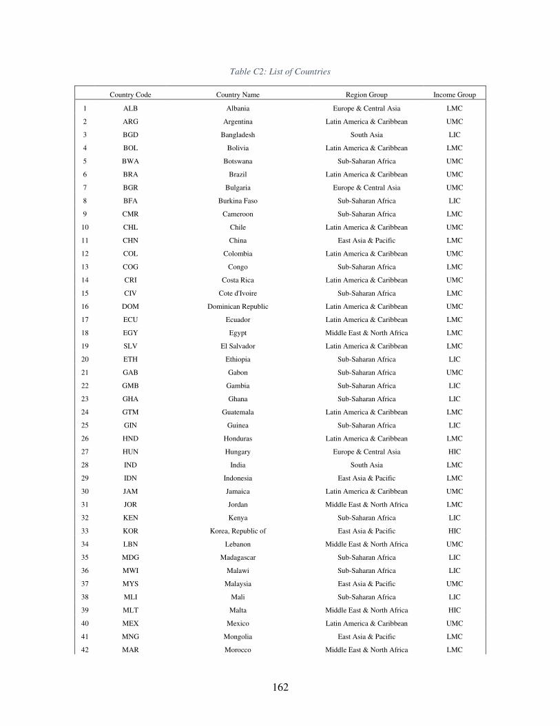
162

Table C2: List of Countries

Country Code Country Name Region Group Income Group

1 ALB Albania Europe & Central Asia LMC

2 ARG Argentina Latin America & Caribbean UMC

3 BGD Bangladesh South Asia LIC

4 BOL Bolivia Latin America & Caribbean LMC

5 BWA Botswana Sub-Saharan Africa UMC

6 BRA Brazil Latin America & Caribbean UMC

7 BGR Bulgaria Europe & Central Asia UMC

8 BFA Burkina Faso Sub-Saharan Africa LIC

9 CMR Cameroon Sub-Saharan Africa LMC

10 CHL Chile Latin America & Caribbean UMC

11 CHN China East Asia & Pacific LMC

12 COL Colombia Latin America & Caribbean UMC

13 COG Congo Sub-Saharan Africa LMC

14 CRI Costa Rica Latin America & Caribbean UMC

15 CIV Cote d'Ivoire Sub-Saharan Africa LMC

16 DOM Dominican Republic Latin America & Caribbean UMC

17 ECU Ecuador Latin America & Caribbean LMC

18 EGY Egypt Middle East & North Africa LMC

19 SLV El Salvador Latin America & Caribbean LMC

20 ETH Ethiopia Sub-Saharan Africa LIC

21 GAB Gabon Sub-Saharan Africa UMC

22 GMB Gambia Sub-Saharan Africa LIC

23 GHA Ghana Sub-Saharan Africa LIC

24 GTM Guatemala Latin America & Caribbean LMC

25 GIN Guinea Sub-Saharan Africa LIC

26 HND Honduras Latin America & Caribbean LMC

27 HUN Hungary Europe & Central Asia HIC

28 IND India South Asia LMC

29 IDN Indonesia East Asia & Pacific LMC

30 JAM Jamaica Latin America & Caribbean UMC

31 JOR Jordan Middle East & North Africa LMC

32 KEN Kenya Sub-Saharan Africa LIC

33 KOR Korea, Republic of East Asia & Pacific HIC

34 LBN Lebanon Middle East & North Africa UMC

35 MDG Madagascar Sub-Saharan Africa LIC

36 MWI Malawi Sub-Saharan Africa LIC

37 MYS Malaysia East Asia & Pacific UMC

38 MLI Mali Sub-Saharan Africa LIC

39 MLT Malta Middle East & North Africa HIC

40 MEX Mexico Latin America & Caribbean UMC

41 MNG Mongolia East Asia & Pacific LMC

42 MAR Morocco Middle East & North Africa LMC

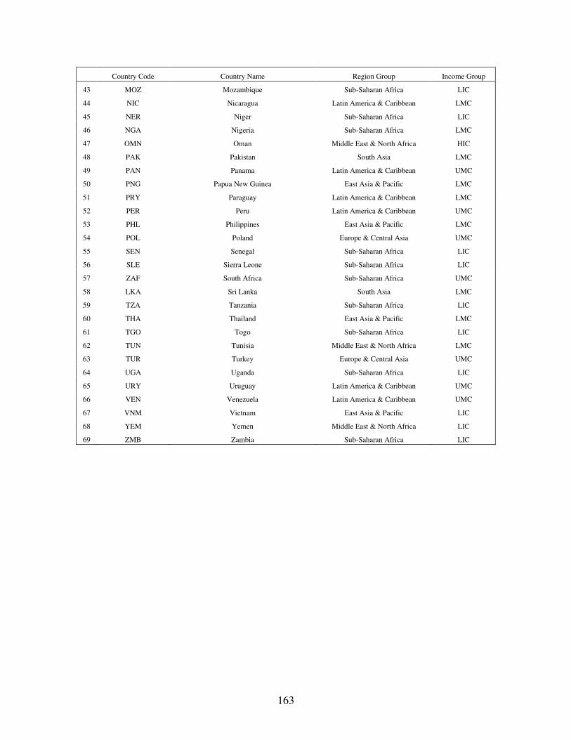
163

Country Code Country Name Region Group Income Group

43 MOZ Mozambique Sub-Saharan Africa LIC

44 NIC Nicaragua Latin America & Caribbean LMC

45 NER Niger Sub-Saharan Africa LIC

46 NGA Nigeria Sub-Saharan Africa LMC

47 OMN Oman Middle East & North Africa HIC

48 PAK Pakistan South Asia LMC

49 PAN Panama Latin America & Caribbean UMC

50 PNG Papua New Guinea East Asia & Pacific LMC

51 PRY Paraguay Latin America & Caribbean LMC

52 PER Peru Latin America & Caribbean UMC

53 PHL Philippines East Asia & Pacific LMC

54 POL Poland Europe & Central Asia UMC

55 SEN Senegal Sub-Saharan Africa LIC

56 SLE Sierra Leone Sub-Saharan Africa LIC

57 ZAF South Africa Sub-Saharan Africa UMC

58 LKA Sri Lanka South Asia LMC

59 TZA Tanzania Sub-Saharan Africa LIC

60 THA Thailand East Asia & Pacific LMC

61 TGO Togo Sub-Saharan Africa LIC

62 TUN Tunisia Middle East & North Africa LMC

63 TUR Turkey Europe & Central Asia UMC

64 UGA Uganda Sub-Saharan Africa LIC

65 URY Uruguay Latin America & Caribbean UMC

66 VEN Venezuela Latin America & Caribbean UMC

67 VNM Vietnam East Asia & Pacific LIC

68 YEM Yemen Middle East & North Africa LIC

69 ZMB Zambia Sub-Saharan Africa LIC

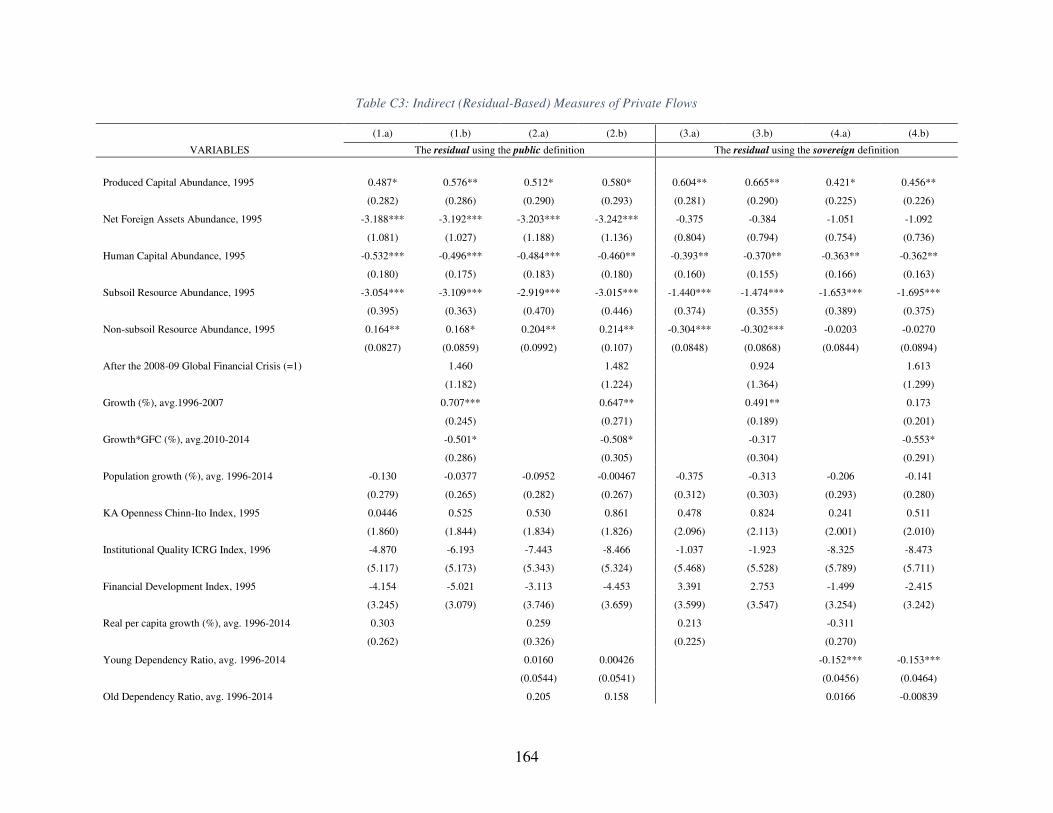
164

Table C3: Indirect (Residual-Based) Measures of Private Flows

(1.a) (1.b) (2.a) (2.b) (3.a) (3.b) (4.a) (4.b)

VARIABLES The residual using the public definition The residual using the sovereign definition

Produced Capital Abundance, 1995 0.487* 0.576** 0.512* 0.580* 0.604** 0.665** 0.421* 0.456**

(0.282) (0.286) (0.290) (0.293) (0.281) (0.290) (0.225) (0.226)

Net Foreign Assets Abundance, 1995 -3.188*** -3.192*** -3.203*** -3.242*** -0.375 -0.384 -1.051 -1.092

(1.081) (1.027) (1.188) (1.136) (0.804) (0.794) (0.754) (0.736)

Human Capital Abundance, 1995 -0.532*** -0.496*** -0.484*** -0.460** -0.393** -0.370** -0.363** -0.362**

(0.180) (0.175) (0.183) (0.180) (0.160) (0.155) (0.166) (0.163)

Subsoil Resource Abundance, 1995 -3.054*** -3.109*** -2.919*** -3.015*** -1.440*** -1.474*** -1.653*** -1.695***

(0.395) (0.363) (0.470) (0.446) (0.374) (0.355) (0.389) (0.375)

Non-subsoil Resource Abundance, 1995 0.164** 0.168* 0.204** 0.214** -0.304*** -0.302*** -0.0203 -0.0270

(0.0827) (0.0859) (0.0992) (0.107) (0.0848) (0.0868) (0.0844) (0.0894)

After the 2008-09 Global Financial Crisis (=1) 1.460 1.482 0.924 1.613

(1.182) (1.224) (1.364) (1.299)

Growth (%), avg.1996-2007 0.707*** 0.647** 0.491** 0.173

(0.245) (0.271) (0.189) (0.201)

Growth*GFC (%), avg.2010-2014 -0.501* -0.508* -0.317 -0.553*

(0.286) (0.305) (0.304) (0.291)

Population growth (%), avg. 1996-2014 -0.130 -0.0377 -0.0952 -0.00467 -0.375 -0.313 -0.206 -0.141

(0.279) (0.265) (0.282) (0.267) (0.312) (0.303) (0.293) (0.280)

KA Openness Chinn-Ito Index, 1995 0.0446 0.525 0.530 0.861 0.478 0.824 0.241 0.511

(1.860) (1.844) (1.834) (1.826) (2.096) (2.113) (2.001) (2.010)

Institutional Quality ICRG Index, 1996 -4.870 -6.193 -7.443 -8.466 -1.037 -1.923 -8.325 -8.473

(5.117) (5.173) (5.343) (5.324) (5.468) (5.528) (5.789) (5.711)

Financial Development Index, 1995 -4.154 -5.021 -3.113 -4.453 3.391 2.753 -1.499 -2.415

(3.245) (3.079) (3.746) (3.659) (3.599) (3.547) (3.254) (3.242)

Real per capita growth (%), avg. 1996-2014 0.303 0.259 0.213 -0.311

(0.262) (0.326) (0.225) (0.270)

Young Dependency Ratio, avg. 1996-2014 0.0160 0.00426 -0.152*** -0.153***

(0.0544) (0.0541) (0.0456) (0.0464)

Old Dependency Ratio, avg. 1996-2014 0.205 0.158 0.0166 -0.00839

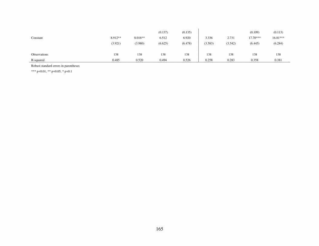
165

(0.137) (0.135) (0.109) (0.113)

Constant 8.912** 8.016** 6.512 6.920 3.336 2.731 17.70*** 16.81***

(3.921) (3.980) (6.625) (6.478) (3.583) (3.542) (6.445) (6.284)

Observations 138 138 138 138 138 138 138 138

R-squared 0.485 0.520 0.494 0.526 0.258 0.283 0.358 0.381


*** p<0.01, ** p<0.05, * p<0.1

DISSERTATION WEALTH COMPOSITION, CAPITAL FLOWS ...

Documents