Dissertation Control of vibrations of civil engineering structures with special emphasis on tall buildings ausgeführt zum Zwecke der Erlangung des akademischen Grades eines Doktors der technischen Wissenschaften unter der Leitung von o.Univ.Prof. Dipl.-Ing. Dr.techn. Dr.h.c. Franz Ziegler E201 Institut für Allgemeine Mechanik eingereicht an der Technischen Universität Wien Fakultät für Bauingenieurwesen von Dipl.-Ing. Markus J. Hochrainer MSc. 1200 Wien, Universumstr. 12/25 Wien, Dezember 2001 Die approbierte Originalversion dieser Dissertation ist an der Hauptbibliothek der Technischen Universität Wien aufgestellt (http://www.ub.tuwien.ac.at). The approved original version of this thesis is available at the main library of the Vienna University of Technology (http://www.ub.tuwien.ac.at/englweb/).

Welcome message from author
This document is posted to help you gain knowledge. Please leave a comment to let me know what you think about it! Share it to your friends and learn new things together.
Transcript

Dissertation
Control of vibrations
of civil engineering structures
with special emphasis on tall buildings
ausgeführt zum Zwecke der Erlangung des akademischen Grades
eines Doktors der technischen Wissenschaften unter der Leitung von
o.Univ.Prof. Dipl.-Ing. Dr.techn. Dr.h.c. Franz Ziegler
E201
Institut für Allgemeine Mechanik
eingereicht an der Technischen Universität Wien
Fakultät für Bauingenieurwesen
von
Dipl.-Ing. Markus J. Hochrainer MSc.
1200 Wien, Universumstr. 12/25
Wien, Dezember 2001
Die approbierte Originalversion dieser Dissertation ist an der Hauptbibliothek der Technischen Universität Wien aufgestellt (http://www.ub.tuwien.ac.at). The approved original version of this thesis is available at the main library of the Vienna University of Technology (http://www.ub.tuwien.ac.at/englweb/).

VI
Contents
1. FUNDAMENTALS 1
1.1. DYNAMIC BEHAVIOUR OF SINGLE -DEGREE-OF-FREEDOM SYSTEMS 1
1.1.1. EQUATION OF MOTION 1
1.2. EQUATIONS OF MOTION FOR LINEAR MDOF STRUCTURES 13
1.3. ENERGY CONSIDERATIONS 17
1.4. STATE TRANSFORMATIONS AND STATE SPACE REPRESENTATION 19
1.5. REFERENCES 22
2. OVERVIEW OF PASSIVE DEVICES FOR VIBRATION DAMPING 24
2.1. METALLIC DAMPERS 24
2.2. FRICTION DAMPERS 25
2.3. VISCOELASTIC DAMPERS 27
2.4. VISCOUS FLUID DAMPERS 28
2.5. DYNAMIC VIBRATION ABSORBERS 30
2.5.1. TUNED LIQUID DAMPERS 30
2.5.2. SEISMIC ISOLATION 33
2.6. TUNED MASS DAMPERS 37
2.6.1. BASIC EQUATIONS 38
2.6.2. DENHARTOG’S SOLUTION FOR OPTIMAL ABSORBER PARAMETER 40
2.6.3. STRUCTURAL IMPLEMENTATIONS 47
2.7. SMART MATERIALS 47
2.7.1. SHAPE MEMORY ALLOYS 48
2.7.2. PIEZOELECTRIC MATERIALS 49
2.7.3. ELECTRORHEOLOGICAL FLUID 51
2.7.4. MAGNETORHEOLOGICAL FLUID 51
2.8. REFERENCES 51

VII
3. STATE OF THE ART REVIEW ON TUNED LIQUID COLUMN DAMPER 55
3.1. REFERENCES 67
4. MATHEMATICAL DESCRIPTION AND DISCUSSION OF THE GENERAL SHAPED TLCD 70
4.1. EQUATIONS OF MOTION FOR PLANE TLCD 70
4.1.1. DERIVATION OF THE EQUATION OF MOTION USING THE
LAGRANGE EQUATIONS OF MOTION 72
4.1.2. BERNOULLI’S EQUATION FOR MOVING COORDINATE SYSTEMS 74
4.1.3. DERIVATION OF THE EQUATION OF MOTION APPLYING THE GENERALISED
BERNOULLI EQUATION 78
4.2. REACTION FORCES AND MOMENTS FOR THE PLANE TLCD 79
4.3. DETERMINATION OF THE AIR SPRING EFFECT 82
4.4. GENERAL DISCUSSION OF THE TLCD’ S DESIGN AND ITS ADVANTAGES 87
4.4.1. INFLUENCE OF GEOMETRY 87
4.4.2. INSTALLATION AND MAINTENANCE 88
4.4.3. IN SITU TESTING OF STRUCTURES 89
4.5. TORSIONAL TUNED L IQUID COLUMN DAMPER (TTLCD) 89
4.5.1. INTRODUCTION 89
4.5.2. EQUATION OF MOTION 90
4.5.3. FORCES AND MOMENTS 92
4.6. REFERENCES 95
5. OPTIMAL DESIGN OF TLCDS ATTACHED TO HOST STRUCTURES 97
5.1. ANALOGY BETWEEN TMD AND TLCD FOR SDOF HOST STRUCTURE 97
5.4.1. APPLICATION OF TMD-TLCD ANALOGY TO SDOF HOST STRUCTURE WITH
TLCD ATTACHED 100
5.2. CONTROL OF MDOF HOST STRUCTURES BY TLCD 103
5.3. GENERAL REMARKS ON TMD-TLCD ANALOGY 107
5.4. REFERENCES 108

VIII
6. EQUATIONS OF MOTION OF LINEAR MDOF STRUCTURES 109
6.1. INTRODUCTION 109
6.2. GENERAL APPROACH 109
6.3. GENERAL APPROACH FOR FRAMED STRUCTURES 110
6.4. KINEMATIC CONSTRAINTS 112
6.5. STATIC CONDENSATION 113
6.6. MODAL TRUNCATION 114
6.7. MODAL REDUCTION 118
6.8. EXAMPLES 122
6.9. REFERENCES 123
7. OPTIMISATION OF MULTIPLE TLCDS AND MDOF STRUCTURAL
SYSTEMS IN THE STATE SPACE DOMAIN 124
7.1. OPTIMISATION FOR FREE VIBRATION OF MDOF STRUCTURE WITH
SEVERAL TLCD INSTALLED 126
7.2. FREQUENCY RESPONSE OPTIMISATION FOR MDOF STRUCTURES WITH
SEVERAL TLCD INSTALLED 129
7.2.1. DETERMINATION OF A PERFORMANCE INDEX IN THE FREQUENCY DOMAIN 129
7.3. STOCHASTIC OPTIMISATION : M INIMUM VARIANCE 132
7.4. COMMENTS ON SYSTEMS WITH MULTIPLE INPUTS 135
7.5. COLOURED NOISE INPUT 135
7.6. REMARKS ON THE NUMERICAL OPTIMISATION AND CHOICE OF INITIAL CONDITIONS 138
7.7. REFERENCES 139
8. ACTIVE DEVICES FOR VIBRATION DAMPING 140
8.1. ACTIVE CONTROL 141
8.2. HYBRID CONTROL 142
8.3. SEMI ACTIVE CONTROL SYSTEMS 144
8.4. ACTIVE TUNED L IQUID COLUMN DAMPER (ATLCD) 145
8.4.1. STATE SPACE REPRESENTATION 149

IX
8.5. OPTIMAL CONTROL 150
8.6. MODAL CONTROL 154
8.7. POLYNOMIAL AND SWITCHING CONTROL LAWS 155
8.8. REFERENCES 158
9. APPLICATION TO REAL STRUCTURES AND NUMERICAL STUDIES 162
9.1. 3D-BUILDING WITH TRANSLATIONAL AND TORSIONAL PASSIVE TLCD 162
9.2. WIND EXCITED 47-STORY TALL BUILDING 176
9.2.1. OPTIMAL TMD DESIGN 178
9.2.2. TLCD DESIGN 180
9.2.3. SIMULATION OF TURBULENT DAMPING 184
9.2.4. DEVICE CONFIGURATION AND CONCLUDING REMARKS 185
9.3. 3-DOF BENCHMARK STRUCTURE 188
9.3.1. INTRODUCTION 188
9.3.2. TLCD DESIGN 189
9.3.3. IMPLEMENTATION OF AN ACTIVE PRESSURE CONTROL 193
9.4. 76-STORY BENCHMARK STRUCTURE 200
9.4.1. RESPONSE OF ORIGINAL BUILDING 203
9.4.2. PASSIVE TLCD 206
9.4.3. PERFORMANCE CRITERIA 213
9.5. BENCHMARK CONTROL PROBLEM FOR SEISMICALLY EXCITED ST RUCTURE 220
9.5.1. TLCD DESIGN 223
9.5.2. ACTIVE CONTROL 226
9.6. REFERENCES 231
APPENDIX 233
A. EQUIVALENT LINEARISATION 233
B. LYAPUNOV EQUATION 235
C. NOTATION 236

1. Fundamentals
1
1. Fundamentals
Traditionally, most civil engineering structures have been designed and considered as static
systems, but the development and application of modern protective elements demands a more
precise analysis. Instead, buildings, towers or bridges must be considered as dynamic systems,
allowing better mathematical modelling and a correct investigation of the dynamic behaviour.
In this introductory section a simple structure is idealised as a single-degree-of-freedom
(SDOF) system with a lumped mass on a supporting structure, thus representing the prototype
of a spring-mass-dashpot system. Such a linear oscillator model permits the investigation of
typical dynamic effects like free and forced vibration, the influence of damping and the
resonance phenomenon. While such a simple model is useful for developing an understanding
of the dynamic behaviour, most real structures must be represented by multiple-degree-of-
freedom (MDOF) systems for better reproduction of the actual structural behaviour. After a
basic treatment of single-degree-of-freedom systems, for which some general analysis
procedures are outlined, the structural modelling is extended to multiple-degree-of-freedom
systems where resonance phenomena, a system representation in state space description as
well as basic concepts, like state transformations and modal analysis are discussed. The
introduction is mainly influenced by presentations included in Ziegler1, Soong and Dargush2,
Chopra3, Clough-Penzien4 and Magnus5.
1.1. Dynamic behaviour of single-degree-of-freedom systems
1.1.1. Equation of motion
The simplest model that demonstrates most essential response characteristics when subjected
to dynamic loading is the single-degree-of-freedom system, for two simple models see Figure
1-1.

1. Fundamentals
2
2k2k k
Kelvin Voigt body
tw
twg twg
tf
tfl
Figure 1-1: Singe degree of freedom model excited by a (wind) force ( )tf and a ground
motion ( )twg : a) shear frame model b) mass-spring-dashpot system
It consists of a mass m concentrated on the roof level and is supported by a massless frame,
providing a total linear elastic stiffness k to the system - the reduced stiffness due to the
vertical loading of the column (P-∆ -effect) is included, and approximately reduces the
unloaded column stiffness k by lgmkk 56−= , where g denotes the constant of gravity
acceleration, see Ziegler6. A linear viscous damper, representing a simple model of material
damping has the viscosity c and is in parallel connection to the Hookean spring thereby
forming a Kelvin-Voigt body. The system is subjected to a seismic disturbance characterised
by a spatially uniform, time-dependent ground acceleration gwɺɺ , and a time dependent single
force ( )tf . The lateral displacement( )tw , relative to the ground, describes the response of
the excited system, and the absolute displacement is
( ) ( ) ( )twtwtw gt += .
( 1-1)
Assuming spring and damping forces linearly proportional to the displacement and the
velocity, respectively, the equation of motion for this SDOF system follows directly from
Newton’s law and can be written as
fwmwkwcwm g +−=++ ɺɺɺɺɺ
( 1-2)

1. Fundamentals
3
in which the differentiation with respect to time is given by the superimposed dots, e.g. in the
material description td
xdx =ɺ or
2
2
td
xdx =ɺɺ . If appropriate, the time argument is skipped in time
dependent quantities to gain clarity in long expressions. It is often convenient to introduce the
effective loading
( ) ( ) ( )tftwmtf geff +−= ɺɺ ,
( 1-3)
so that it is not necessary to distinguish between force loading and ground excitation.
1.1.1.1. Free vibrations
A structure is said to perform free vibration if it is disturbed from its equilibrium position and
then allowed to vibrate without any external dynamic excitation. In absence of any effective
loading, the right hand terms of Eq. ( 1-2) vanish and it simplifies to the case of natural
vibration. If the mass is given some initial displacement ( )0w and velocity ( )0wɺ the response
of the SDOF system becomes
( ) ( ) ( )101 cosexp φωζω −−= ttwtw Dh
( )
( ) ( )
( )0
00
1
1tan 0
2121 w
ww ζω
ζφ
+
−=
ɺ
, ( ) ( ) ( ) ( ) 21
20
2
20
210
1
1020
1
0
−+
+
−=
ωζωζ
ζww
ww
wɺɺ
( 1-4)
( 1-5)
where Dω and ζ represent the damped natural circular frequency and the nondimensional
damping ratio given by
2
0 1 ζωω −=D , 12 0
<=ω
ζm
c.
( 1-6)
and 0ω denotes the natural circular frequency of the undamped structure, defined as
000
22
Tf
m
k ππω === ,
( 1-7)
Notice, that for 0=ζ , the free vibration response Eq.( 1-4) does not decay and in absence of
dissipation the motion is characterised by the perpetual exchange of potential (strain) and

1. Fundamentals
4
kinetic energies. Damping has the effect of lowering the natural circular frequency from 0ω
to Dω and lengthening the natural period from 0T to DDT ωπ2= . These effects are
negligible for damping ratios ζ below 20%, a range that includes material damping of all
civil engineering structures of interest. Increasing ζ to the critical damped value 1== critζζ
changes the response character completely, since Dω becomes complex and the system
response Eq. ( 1-4) looses its vibrational characteristics. Instead, the structural response of
such an over-critically damped system is described by two decaying exponential functions,
obtained from the sine and cosine functions with complex arguments. However, those highly
damped systems do not occur in the elastic deformation range of civil engineering structures.
Common damping ratios for steel, concrete and wooden structures are between %5.0=ζ and
%3=ζ , presuming linear elastic behaviour. Figure 1-2 illustrates the SDOF system’s
displacement in natural vibration for various damping factors with the initial conditions
0)0( wwh = and 00)0( wwh ω=ɺ .
0 1 2 3 4 5 6 7 8 9 10-2
-1
0
1
2
ζ=0
ζ=0.01
ζ=0.05
ζ=0.2envelope
0w
w
0Tt
te 0ζω−
Figure 1-2: Free vibration response for various damping ratios
1.1.1.2. Forced vibrations – time harmonic forcing
The response of SDOF systems to harmonic excitation is a classical topic in structural
dynamics, not only because such excitations often occur in engineering systems, but because

1. Fundamentals
5
the frequency response function provides indeed insight, how the system will respond to more
general time dependent forces. At this point it is useful to distinguish between the excitation
due to a pure force loading and the vibrations caused by a ground motion.
1.1.1.3. Force loading
Firstly, in the case of forced vibrations, let the ground acceleration gwɺɺ be put to zero, thus,
effective forcing becomes ( )tffeff ωcos0= . Consequently, a time-harmonic force of
magnitude 0f and frequency ν excites the SDOF model. This effective loading can also be
described by the real part of the complex exponential function
( ) ( )
<≥=
=0for 0
0forcosRe 00
t
ttfeff
ti
eff
νν
( 1-8)
with 1−=i representing the imaginary unit. Due to the superposition principle, the total
response can be given as sum of the homogenous and a particular solution
( ) ( ) ( )twtwtw ph += ,
( 1-9)
Starting with homogenous initial conditions the solution of Eq.( 1-2) due to the harmonic force
is obtained in the complex form:
( ) ( ) ( ) ( )22011 expexpexp φωωζφν −−+−= tiwttiwtw D ,
( 1-10)
in which 1w , 2w , 1φ and 2φ denote amplitudes and phase angels, respectively, which are
given by,
( ) ( )( ) 21222
01
21
1
γζγ +−=
k
fw ,
2
12
1 ζ−= w
w
211
2tan
γζγφ
−= , ( ) γ
γζζφ
−+
−=
1
1
1tan
2122
( 1-11) ( 1-12)
γ denotes the ratio of the forcing to the undamped natural frequency,
0ωνγ = .
( 1-13)

1. Fundamentals
6
The first term appearing in Eq.( 1-10) corresponds to the steady-state solution, whereas the
second describes the transient response component, which might be responsible for peaks in
the transient regime. Due to damping the amplitude of transient response decays and, after
several periods, the steady-state term will cause the dominant response contribution.
Referring the steady state displacement amplitude 1w to the static displacement stw defines
the response function, ( )γdA , for real input
( ) ( ) ( ) ( )[ ] ,21exp 1211 −
+−=−= γζγφγγ i
w
iwA
std
k
fwst
0= .
( 1-14)
( 1-15)
The absolute value of ( )γdA is called amplitude response function and measures the
amplitude magnification when compared to the static load case, whereas phase angle between
the excitation and the response is described by the phase shift ( )( )γdAarg . Both quantities are
respectively given by
( ) ( ) ( ) 2
1
222 21−
+−= γζγγdA ,
( )( )
−= −
2
1
1
2tanargγγζγdA ,
( 1-16) ( 1-17)
and they are of vital interest for dynamic analysis. The amplitude response magnification can
e.g. be used to determine local stress distributions to estimate the possibility of material
fatigue, even within elastic limits: the admissible stress amplitude decreases with the number
of load cycles according to Wöhler’s curve, see e.g. Chwalla7
1.1.1.4. Ground excitation
The second loading case, by ground excitation, can be treated analogously, if the effective
force excitation is given by the ground excitation forcing ( )twf geff νν cos2−= . Thus the
solution can be given by Eq.( 1-10), when replacing 0f by efff .

1. Fundamentals
7
When referring the steady state response to the ground excitation input gw , it is possible to
define the complex displacement frequency response function
( ) ( )[ ] 12 21−
+−= gggd iA γζγγ
( 1-18)
Again, the absolute values of ( )νdA and the phase shift ( )( )νdAarg are
( ) ( ) ( ) 2
1222 21
−
+−= gggdA γζγγ , ( )( )
−= −
21
1
2tanarg
g
ggdA
γγζγ ,
( 1-19)
but in contrast to the force loading of Section 1.1.1.3 the reciprocal nondimensional excitation
frequency gγ is defined as
νωγγ 01 == −
g .
( 1-20)
1.1.1.5. Resonant vibrations
Apparently, Eq.( 1-14) and Eq.( 1-18) are identical but the difference between the two
excitation types lies in the definition of the non-dimensional frequency γ , namely of
Eq.( 1-13) and 1−= γγ g of Eq.( 1-20). As it is either defined by 0ων or reciprocally by νω0 ,
the response functions are mirrored about the resonance frequency 1=γ . Besides the
displacement response curve, the frequency response curves of the velocity ( ) ( )γγγ dv AiA =
and of the acceleration ( ) ( )γγγ da AA 2−= , are of equal importance, when characterising
dynamic systems. It is understood, that gγ has to be substituted in case of base excitation. All
frequency response curves are represented parametrically with respect to the damping
coefficient, in a fourfold logarithmic diagram named after Blake, see Figure 1-3a.

1. Fundamentals
8
Figure 1-3: a) Blake’s diagram: Amplitude frequency response function of displacement, velocity and acceleration b) Phase frequency response of the steady state vibrations, see
Ziegler1
Under steady state conditions, the maximum displacement magnification occurs at the
resonance frequency Dω and is given by
( )[ ]212
1max
ζζγ
−=dA .
( 1-21)
For weakly damped systems 2.0<ζ it can be approximated by ( )[ ] ζγ 21max =dA . Figure
1-3b displays the phase frequency response curves parametrically with respect to the
damping. The phase shift at resonance is always 2π , which is of practical value if a
resonance has to be determined experimentally. The resonance magnification is only limited
by damping, e.g. for 01.0=ζ the amplification factor is approximately 50 whereas for
2.0=ζ it decreases to 2.5, for structures with identical static behaviour. It is often helpful to
work with a slightly modified notation of the frequency response function where absolute
frequencies replace the non-dimensional frequencies γ or gγ . The simple relation
( )
=
0ωνν dAH ,
( )
=
gdg AH
νων 0 ,
( 1-22)
ω0/ν ω0/ν

1. Fundamentals
9
can be utilised to obtain the frequency response function ( )γH or ( )gH γ .
1.1.1.6. Transient resonant vibrations
If a resonant harmonic force excitation of amplitude 0f is applied to a lightly damped SDOF
system at rest, then the amplitudes 1w and 2w of Eq.( 1-11), and the phase angles 1φ and 2φ of
Eq.( 1-12) can be approximated by
ζ2
1021 k
fww ≈= ,
21
πφ = , 22
πφ −=
( 1-23)
where 0ωω ≈D and 1<<ζ . Inserting into Eq.( 1-10) renders the resonant transient vibration
response,
( ) ( )( ) ( )ttk
ftwres 00
0 sinexp12
1 ωωζζ
−−= ,
( 1-24)
For an undamped system, 0=ζ , Hospital’s rule must be applied to obtain
( ) ( )tt
k
ftwres 0
0 sin2
ωω= ,
( 1-25)
which describes an increasing unbounded vibration. For 0>ζ Figure 1-4 visualises the
transient vibration’s envelope function. Another transient phenomenon for undamped SDOF
oscillators is the beat-like-vibration, if the excitation and the natural frequency only differ
slightly. In this case Eqs.( 1-11) and ( 1-12) render 2
021 1
1
γ−==
k
fww , and 01 =φ , πφ =2 ,
respectively. Inserting into Eq.( 1-10) and applying the additive theorem for harmonic
functions renders
( ) ( )
+
−−
−= ttk
ftw DD
p 2sin
2sin
1
12
0
0 ωνωνων
.
( 1-26)
Figure 1-1 displays such a beating vibration for an undamped system, 0=ζ and
ωνων +<<− .

1. Fundamentals
10
0 2 4 6 8 10 12 14 16 18 200,0
0,2
0,4
0,6
0,8
1,0
1,2
ζ=0.01
ζ=0.05
ζ=0.2
ζ21
st
res
w
w
0Tt
Figure 1-4: Envelope functions of transient resonant vibrations
0 2 4 6 8 10 12 14
-2
-1
0
1
2
3
system responseenvelope functionenvelope function
( )201
1
ων−st
res
w
w
−t
2sin2
ων
0Tt
Figure 1-5: Beat-like-vibration of SDOF oscillator with 0ων ≈
1.1.1.7. Arbitrary periodic forcing function
If the effective excitation is a periodic function ( ) ( )Ttftf effeff += with T defining the
excitation period, it can be expanded in the complex Fourier time series,

1. Fundamentals
11
( ) ∑∞
−∞=
=n
ieff tnT
iCmtf
π2exp . The excitation may then be considered termwise, and the
solutions given in Section 1.1.1.2 are applied to each term and finally, superposition allows to
render the total response. This approach permits the investigation of all steady state vibration
problems by summation of the individual contributions
( ) ∑∞
−∞=
=n
ip tnT
i
TnHCtw
ππ 2exp
2,
( 1-27)
where ( )γH denotes the amplitude response function for force excitation given by Eq.( 1-22).
If force loading and ground excitation are applied simultaneously, then both load cases can
also be treated independently and superimposed to obtain the total response. In practice, the
forcing is considered band-limited, and only a finite number of terms is involved in the above
series representations.
1.1.1.8. Forced vibrations - non-periodic forcing function – transient response
Contrary to the discrete spectrum of a periodic force, the non-periodic forcing function ( )tfeff
has a continuous spectrum, according to the Fourier integral,
( ) ( ) ( )∫∞
∞−
−= dttitfm
c eff ωω exp1
,
( 1-28)
with the continuous Fourier coefficients ( )ωc . The continuous formulation of the
superposition principle in the frequency domain becomes
( ) ( ) ( ) ( )∫∞
∞−
= ωωωωπ
dtiHctw exp2
1,
( 1-29)
where ( )ωH denotes the complex frequency response function, Eq.( 1-22). The integrals in
Eqs.( 1-28) and ( 1-29) can be evaluated by means of the Fast Fourier Transform (FFT), see
e.g. Walker8. The corresponding solution in the time domain for 0>t is given by Duhamel’s
convolution integral, if homogeneous initial conditions of the structure at rest are assumed,
( ) ( ) ( )∫t
eff dthftw0
τττ −= ,
( 1-30)

1. Fundamentals
12
where the impulse response function ( )τ−th defines the displacement at time t due to a unit
impulse force ( ) ( )ttfeff δ= , acting at time τ . In terms of the frequency response function it
is given by
( ) ( ) ( )∫∞
∞−= ωωω
πdtiH
mth exp
2
1,
( 1-31)
and becomes the Green’s function of Eq.( 1-2),
( ) tm
eth D
D
t
ωω
ζω
sin0−
= for 1<ζ ,
( 1-32)
in the case of a SDOF oscillator. For simple excitations the integral expression Eq.( 1-30) can
be solved analytically with the aid of symbolic algebra programs. In general, the convolution
integral must be solved numerically, a task which has become a standard problem in
numerical mathematics. However, using the addition theorem,
( ) τττ sincossincossin ttt −=− , simplifies the evaluation of Eq.( 1-30).
1.1.1.9. Response with a passive damper attached
The previous section has shown the beneficial effects of passive energy dissipation by a linear
viscous damper. However, there are many more mechanisms for energy dissipation like
yielding, friction, radiation damping into the foundation or other types of energy transmission.
Energy loss by those effects cause damping and can be incorporated into the mechanical
model by a general damping element, typically described by a force-displacement relation. If
the dynamic modulus, see e.g. Harris9, is the ratio between the force and the displacement,
w
f=D ,
( 1-33)
then most damper and absorber configurations can be described by the integro-differential
operatorD . In Figure 1-6 such a general damping device is added to the SDOF model. For its
application to multiple story high rise buildings, see e.g. Lei10

1. Fundamentals
13
2kΓ
tf
D
2k
twg
Figure 1-6: SDOF system with general damping device
Writing the force contribution of the device as w⋅D permits various response characteristics
including displacement, velocity and acceleration dependency. Neglecting the mass of the
damping device the extension of Eq.( 1-2) takes on the simple form
efffwwkwcwm =+++ Dɺɺɺ .
( 1-34)
Only if the damping device is purely viscous the energy dissipation of the SDOF model is
always increased which corresponds to an increase in the overall damping ratio. For all other
types of damping devices only careful dynamic analysis can guarantee improved
performance.
1.2. Equations of motion for linear MDOF structures
A proper mathematical idealisation of a physical construction is crucial for the development
of vibration absorbers and the determination of the dynamic characteristics of any structure.
Unfortunately it is rarely adequate to utilise a SDOF idealisation for the entire construction.
Thus the dynamic investigations must be adapted for MDOF structures. Although the
structural model can have several degrees of freedom, the structure-soil-structure interaction
is not accommodated for, and the ground excitation in vertical direction is neglected
throughout this dissertation. Figure 1-7 displays typical idealised lumped mass MDOF
structures, a plane shear frame building, and a cantilevered shear-beam model.

1. Fundamentals
14
1m
2m
3m
4m
5m
1w
2w
3w
4w
5w
1f
2f
3f
4f
5f 5m
3w
5w
1w
2w
4w
1f
2f
3f
4f
5f
4m
3m
2m
1m
twg twg
Figure 1-7: Multiple-story model: a) shear frame b) beam model, both in single point excitation and (wind) force loading
One of the most appropriate techniques for a MDOF discretisation of a continuos structure is
the Finite Element Method (FEM), where, from a physical point of view, each structural
member is mathematically represented by an element having the same mass, stiffness and
damping characteristics as the original member. Those elements are assembled together,
according to the physical construction, rendering a N -DOF system with a discrete set of
variables. The mass, stiffness and damping matrices and a general displacement vector w is
generated during this process. Then, the N equations of motion for the discretised structural
system, under uniform ground excitation and time varying forces, can be written analogous to
Eq.( 1-34), in matrix notation,
frMwwKwCwM +−=+++ gs wɺɺɺɺɺ D ,
( 1-35)
where M , C ,K and sr represent the mass, damping, stiffness matrices as well as the static
influence vector, respectively. gwɺɺ and f denote the ground excitation and the dynamic
loading forces, respectively, which can be combined in an effective loading term
frMf +−= gSeff wɺɺ . If additional damping devices are installed, they can be treated analogous
b) a)

1. Fundamentals
15
to SDOF freedom systems by adding the vector expression wD , which again describes
force-displacement relations, for a practical application, see again Lei10. In general, the
stiffness matrix is symmetric ( )jiij kk = whereas such a property does not always exist for the
mass matrix. For linear systems and linear energy dissipating devices it is convenient to
incorporate wD directly into the equations of motion, resulting in modified mass, stiffness
and damping matrices. Due to the increased computational capacity of modern computers, it
is possible to solve Eq.( 1-35) directly. Nevertheless, deep insight can be gained and the
required effort can be kept to a minimum if the equations are uncoupled via a modal
transformation. As such a transformation is normally performed for the main structure, the
additional damping terms wD are not considered and Eq.( 1-35) is solved for undamped free
vibrations via the general solution ( ) tiet ωφw = . This renders the associated generalised
eigenvalue problem,
( ) 02 =− φMK ω ,
( 1-36)
and there are numerous methods available to solve the generalised eigenvalue problem, see
e.g. Stoer11. An N -DOF system will have N nontrivial solutions of Eq.( 1-36), where iω and
iφ denote the corresponding natural frequencies assumed to be well separated, and mode
shape vectors, respectively. Normally the mode shape vectors are sorted according to their
natural frequencies in ascending order, starting with the fundamental mode. When properly
normalised the mode shapes satisfy the following orthogonality conditions
ijjTi δ=φMφ ,
≠=
=ji
jiij
Ti
for0
for2ω
φKφ ,
( 1-37)
( 1-38)
where ijδ represents the Kronecker Symbol. Introducing a linear transformation such that the
original displacements w are expressed by
qΦw =
( 1-39)
where the shape vectors iφ form the columns of the modal matrix (square matrix)
],,[ 1 NφφΦ ⋯= . The modal vector q contains the new generalised, so called principal

1. Fundamentals
16
coordinates. Inserting Eq.( 1-39) into Eq.( 1-36) pre-multiplying with the transposed modal
matrix TΦ and applying Eqs.( 1-37) and ( 1-38) render the following set of equations of
motion in modal coordinates
fΦrMΦqΩqΦCΦq TgS
TT w +−=++ ɺɺɺɺɺ 2 ,
( 1-40)
where ),,( 221
2Ndiag ωω ⋯=Ω . The simultaneous diagonalisation of a damped system is only
possible, see e.g. Hütte12, Müller13, if the condition
CMKKMC 11 −− =
( 1-41)
holds. This condition is valid for all modally damped systems, also referred to as classically
damped systems. In such a situation the transformed damping matrix ΦCΦT is also of
diagonal shape and the left hand side of the damped structural system, Eq.( 1-40), decouples
completely. Since very little is known about the actual damping conditions in a building,
modal damping is frequently introduced into the equations of forced motion. The special case
of the proportional Rayleigh damping
KMC 21 αα += ,
( 1-42)
e.g., allows modal decoupling, but it can be generalised to the Caughey series, see Soong2,
p.22,
( )∑−
=
−=1
0
1N
j
jj KMMC α
( 1-43)
Using the normalisation condition, Eq.( 1-37), and expanding Eq.( 1-43), renders
( )
( ) ( )
⋯
222
1111111
2
10
11
210
ΩIΩIΩ
ΦKΦΦMΦΦKΦΦMΦΦKΦ
ΦKΦΦMΦ
ΦKMKΦΦKΦΦMΦΦCΦ
d
TTTTTN
jj
TT
jN
j
Tj
TTT
−−−−−−−
=
−−
=
∑
∑
+
+=
++=
α
αα
ααα
[ ] ( )∑−
===
1
01111
2 2,,2N
j
jj diag ωζωζα ⋯Ω ,
( 1-44)
( 1-45)

1. Fundamentals
17
where jζ denote the modal damping ratios. Under the condition of separated natural
frequencies Eq.( 1-45) has a solution for the damping coefficients jα . The damping matrix of
a 3-DOF model, e.g., can be given by
( )∑=
−=2
0
1
j
jj KMMC α ,
( 1-46)
where
=
−
−
−
−
3
2
1
1
333
13
322
12
311
11
2
1
0
2
ζζζ
ωωωωωωωωω
ααα
.
( 1-47)
After the modal transformation is performed, the equations of motion simplify to a set of
scalar equations, one for each mode j
fφ
Tjg
jgjjjjjj wqqq +−=++ ɺɺɺɺ ξωωζ 22 , Nj ,,2,1 ⋯=
STj
jg rMφ=ξ
( 1-48)
( 1-49)
where jq and jgξ denotes the modal coordinate and the participation factor of the ground
acceleration, respectively. Besides the participation factor, the first excitation term depends on
the spectral density of the ground excitation. The second excitation term depends on spatial
distribution of f and on time. Equation ( 1-48) is identical with a SDOF equation of motion
with effective forcing, and consequently all methodology and phenomena developed and
discussed in Section 1.1.1.1 to Section 1.1.1.9 are applicable. The major computational task is
the determination of the natural frequencies and the mode shape vectors. For large systems,
however, often only the structural modes within the lower frequency band need to be
calculated, and a diagonalisation is performed before the dynamic analysis.
1.3. Energy considerations
Traditionally, the calculation of displacements, velocities, accelerations and forces has been
of outmost interest during design and investigation of dynamic resistance. However, with the
development of innovative concepts in passive energy dissipation a focus on energy as a
design criterion has been developed. This line of attack puts the centre of attention towards

1. Fundamentals
18
the need to dissipate structural energy instead of increasing the resistance to lateral loads.
Energy considerations are very general in nature and appropriate to incorporate dynamic
effects due to various load cases e.g. wind or seismic loading. The resulting formulation is
suitable for a general discussion of energy dissipation and used in the chapter about the tuned
liquid column damper (TLCD) design optimisation with performance indices, see Chapter 7.
In the following section an energy formulation for the idealised SDOF and MDOF system is
developed which may include one or more passive devices. A straightforward energy
approach is the integration of the equations of motion over the entire displacement history. As
a result one obtains, see Soong2,
IPSDKin EEEEE =+++
( 1-50)
where the individual energy expressions are given by
wMw ɺɺ2
1=kinE ,
∫= dtE TD wCw ɺɺ ,
wKwwKw TTS dE
2
1== ∫ ,
( ) ww dE TP ∫= D ,
∫ ∫ wfwMw ddE TgI +−= ɺɺ .
( 1-51)
( 1-52)
( 1-53)
( 1-54)
( 1-55)
The contributions on the left hand side of Eq. ( 1-50) represent the relative kinetic energy kinE ,
the dissipative energy DE caused by light material damping of the structure with viscous
module, and the elastic strain energySE . PE denotes the energy dissipated via the general
damping device. From the law of conservation of mechanical energy it can be concluded that
the sum of these energies balances the external input energy IE , which comprises of the
energy input due to seismic activity and the wind energy. From an energy perspective, one
must attempt to minimise the amount of kinetic and strain energy by proper design. Two
approaches are feasible. The first reduces the energy input into the structure, like base
isolation, whereas the latter focuses on the application of additional energy dissipating
mechanism in the structure, which is the central theme of this thesis. The main goal is to avoid

1. Fundamentals
19
any damage caused by excessive loading (plastic deformation, overturning moments, P-∆-
effect, etc) of the main structure by the installation of energy consuming substructures.
1.4. State transformations and state space representation
The linear equations of motion of an arbitrary linear time invariant structural system are
second order differential equations, resulting from conservation of momentum,
efffwKwCwM =++ ɺɺɺ ,
( 1-56)
with an effective load vector, frMf +−= gSeff wɺɺ , see Section 1.1.1.7 for wind and seismic
load. Often w describes the absolute deformations, but many other sets of coordinates are
possible, e.g. the relative story displacements. Any physically meaningful coordinates can be
obtained from w by the regular state transformation
wTw 1−= ,
( 1-57)
with the regular transformation matrix T . A special case is the modal transformation where
ΦT = , yielding a diagonal mass and stiffness matrix when pre-multiplying with TΦ . The
equation of motion in transformed coordinates becomes
efffwTKwTCwTM =++ ɺɺɺ
( 1-58)
Working with a set of first order differential equations often simplifies dynamic system
analysis, and a suitable representation of Eq.( 1-56) can be achieved by introducing a new state
variable z consisting of the displacements and velocities of the original system, Eq.( 1-56):
( )
=
w
wz
ɺt .
( 1-59)
With this new state vector Eq.( 1-56) can be rewritten as a system of first order differential
equations:

1. Fundamentals
20
( ) ( ) ( )
+
−−= −−−−−− t
ttefffMT
0z
TCMTTKMT
I0z 111111ɺ .
( 1-60)
Eq.( 1-60) is known as the state space representation of the dynamic system, Eq.( 1-56). It is
not limited to linear systems. The inversion of the mass matrix is always possible, unless the
original set of equations, Eq.( 1-56), contains algebraic equations which must be solved before
performing the transformation. Any state space representation is equivalent to the equations of
motion, but the reduction from a second to a first order system comes at the price that the new
system dimensions are twice the original ones. Of course another state transformation zTz =
can be applied if desired. State space representations have become widely used and
appreciated, since many powerful mathematical tools can be applied directly, and it is the
favourite description of dynamic system in control engineering. If necessary, the state space
equations are extended by a so called ‘output equation’ which is a function of the state and the
external excitation, for linear systems
( ) ( ) ( )ttt efffDzCy += .
( 1-61)
Such an output equation is particularly useful if one is not interested in all state variables but
in particular output quantities, e.g. certain floor accelerations, velocities, displacements or a
combination of those like shear forces or moments and torques.
In system analysis, Eqs.( 1-60) and ( 1-61) are often written in a standardised form given by
( ) ( ) ( )ttt efffBzAz +=ɺ ,
( ) ( )tt efffDzCy += ,
( 1-62)
where A , B , C and D are denoted system matrix, input, output and feed-through matrix,
respectively. It is vital to be aware of the outstanding importance of the system matrix: all
relevant information about dynamic behaviour e.g. free vibration response, damping and
stability, pole location, is contained in A . For that reason the system matrix plays the very
central role in system analysis. Transforming Eq.( 1-62) into the Laplace domain,
( ) ( ) ( )∫∞
−==0
dtetfsftf tsL , see e.g. Doetsch14, and solving for ( )sZ yields
( ) ( ) ( ) ( ) ( )011 zssss eff−− −+−= AIFBAIZ ,
( 1-63)

1. Fundamentals
21
( ) ( )( ) ( ) ( ) ( )011 zssss eff−− −++−= AICFDBAICY ,
The inverse Laplace transformation is given by
( ) ( ) ( ) ( )
<>
=== ∫∞+
∞− 0für 0
0für
2
11-
t
ttfdsesf
itfsf
i
i
tsδ
δπL
( 1-64)
where the complex variable s is defined by νδ is += , and the state transition matrix ( )tΓ is
defined as the inverse Laplace transformation of the resolvant matrix ( )sΓ :
( ) ( ) 1−−= AIΓ ss ,
( ) ( ) st ΓΓ -1L= ,
( 1-65)
By means of the inverse Laplace transformation, Eq.( 1-63), and the convolution theorem,
( ) ( ) ( ) ( )∫ −=⋅−t
dtffsfsf0
21211 τττL , the time domain solution can be given by
( ) ( ) ( )∫ ( ) ( )00
ztdttt
eff ΓfBΓz +−= τττ ,
( ) ( ) ( )∫ ( ) ( ) ( )00
zttdtt eff
t
eff ΓCfDfBΓCy ++−= τττ .
( 1-66)
There are efficient numerical schemes to calculate the state transition matrix. One is using the
Taylor series expansion, see e.g. Müller15, Ludyk16,
( ) ∑∞
=
==0 !n
nnt
n
tet
AΓ
A .
( 1-67)
The system matrix uniquely defines the state transition matrix and this is another proof of the
exceptional importance of A . For linear systems a lot of system design and analysis is done
in the frequency domain, due to the existence of the superposition principle. The input-output
behaviour of dynamic systems, is usually described by the transfer function ( )sH , whose
magnitude and phase angle are called the frequency response of the system. From Eq. ( 1-63)
it follows directly that for homogenous initial conditions the frequency transfer function ( )sH
is given by
1. Fundamentals
22
( ) ( ) ( )sss effFHY = , ( ) ( ) DBAICH +−= −1ss .
( 1-68)
If the output ( )sY is a function of the state variables only (e.g. velocities and displacements),
then 0=D and their is no direct dependence of ( )sY on the input. If furthermore, the output
matrix C is chosen to be the identity matrix, then the frequency response function simplifies
to
( ) ( ) BAIH 1−−= ss .
( 1-69)
Under the assumption that ( )sH can still be computed if the real part of s is chosen to be
zero, s becomes νis = , and it can be written in the equivalent form ( ) ( ) BAIH 1−−= νν ii .
As it describes the system-response to a unit impulse excitation ( ) 1=tδL , the
corresponding time function of ( )sH is normally referred to as the impulse response function,
see Eq.( 1-32) for SDOF oscillators. Since ( ) 0H =t for 0<t , the Fourier transformed, if
existing (see Doetsch14), equals the Laplace transformed with
( ) ( ) ( ) ( )∫∫∞
−
=
∞−
↑===
00
dtetdtetst ti
is
ts ν
νHHHHL ,
( ) ( ) ( ) ( )∫∫∞
−∞
∞−
− ===0
dtetdtett titi ννν HHHHF .
( 1-70)
However, it has to be pointed out that, for general system analysis, the application of the
Laplace transformation is much more powerful, when compared to the Fourier integral.
1.5. References
1 Ziegler, F., Mechanics of Solids and Fluids, 2nd reprint of second edition, Springer, 1999. 2 Soong, T.T., Dargush, G.F., Passive Energy Dissipation Systems in Structural Engineering, Wiley, Chichester
England, 1997 3 Chopra, A.K., Dynamics of Structures, Prentice Hall, New Jersey, 1995 4 Clough, R.W., Penzien, J., Dynamics of Structures, 2nd edition, McGraw-Hill,1993 5 Magnus, K., Popp, K., Schwingungen, 5th. ed., Teuber, Stuttgart, 1997 6 Ziegler, F., Vorlesungen über Baudynamik, lecture notes, Technical University of Vienna, 1979

1. Fundamentals
23
7 Chwalla, E., Introduction to Structural Mechanics, in German, Stahlbau Verlag, Köln, 1954, 8 Walker, J.S., Fast Fourier Transform, CRC Press, 1991 9 Harris, M., Crede, C.E., Shock and Vibration Handbook, McGraw-Hill, 1961 10 Lei, Y., Sure and Random Vibrations of Simple Dissipative Civil Engineering Steel Structures, Dissertation
and Report, Institute of Rational Mechanics, TU-Vienna, A-1040 Wien, Austria, 1994 11 Stoer J., Burlisch R., Numerische Mathematik 2, 3rd edition, Springer Verlag, 1990 12 Hütte, Die Grundlagen der Ingenieurwissenschaften, 29th edition Springer Verlag, 1991 13 Müller, P.C., Stabilität und Matrizen, Springer Verlag Berlin, 1977 14 Doetsch, G., Anleitung zum praktischen Gebrauch der Laplace Tranformation, Oldenburg, 1956 15 Müller, P.C., Stabilität und Matrizen, Springer-Verlag, 1977 16 Ludyk, G., Theoretische Regelungstechnik I, Springer, 1995

2. Overview of passive devices for vibration damping
24
2. Overview of passive devices for vibration damping
The purpose of this chapter is to review common structural control techniques and
applications. It is restricted to passive energy absorbing devices, starting with well established
damping devices like metallic dampers, friction dampers, viscoelastic dampers or viscous
fluid dampers. Section 2.5 is conceptually concerned with dynamic vibration absorbers,
including the description of tuned liquid damper and the shortly described idea of base
isolation. Tuned mass damper are discussed in much more detail (Section 2.6) since the
understanding of their working principle is the basis for the analysis of tuned liquid column
dampers. The chapter ends with a short overview of smart materials used for structural
control.
2.1. Metallic Dampers
One of the most effective mechanisms available for the dissipation of energy already
accumulated in a structure, is through inelastic deformation of metals. In traditional steel
structures the aseismic design relied on the plastic deformation (and post yield ductility) of
structural members whereas the introduction of metallic yield dampers started with the
concept of utilising separate metallic hysteretic dampers to absorb a major part of the external
energy input to the structure. During the years a variety of such devices has been proposed,
many of them using mild steel plates with triangular or hourglass shape so that yielding
spreads evenly throughout the material. The dissipating effect is based on the nonlinear force-
displacement behaviour, which typically contains hysteresis loops for energy dissipation, see
Figure 2-1, where several load cycles with increasing amplitude displacement are displayed
for the Ramberg-Osgood model, see Wen1 for details. Many different designs and materials,
such as lead and shape memory alloys, have been developed and evaluated, some with
particularly desirably features like stable hysteretic behaviour, long term reliability and
insensitivity to environmental temperature. The ongoing research has resulted in the
development of several commercial products for both, new and retrofit construction projects.
The inelastic deformation of metallic elements is the underlying dissipative mechanism for all
different types and geometries of metallic dampers. In order to include these devices in the
structural design, the expected hysteretic behaviour under arbitrary cyclic loading has to be

2. Overview of passive devices for vibration damping
25
characterised. Ideally such a description would be based on the micro-mechanical theory of
dislocations which determine the inelastic response, but since this approach is hardly feasible
a phenomenological description of the processes is accepted. A common approach to describe
the inelastic behaviour of metallic dampers starts with the selection of a basic hysteretic
model, followed by a parameter identification, where curve fitting is utilised to match the
model with experimental data, available from experiments. Additionally, scaling and material
relationships can be determined by macroscopic mechanical analysis of the device.
-6 -4 -2 0 2 4 6-6
-4
-2
0
2
4
6
Strain [%]
Stress
Figure 2-1: Force displacement response of hysteretic model, see Wen1
Since its application in New Zealand 1980, reported in Sinner et al2 , metallic yield dampers
have been installed in various countries, including a 29-storey building in Italy, see Chiampi3,
seismic retrofit installations in USA, see Perry et al.4 and Mexico, see Martinez-Romero5, and
a number of installations in Japan.
2.2. Friction Dampers
Dry friction provides another excellent mechanism for energy dissipation, and plays an
important role in automotive brakes. Based upon an analogy to the automotive brake, began
the development of passive frictional dampers to improve the seismic response of structures.
Although a variety of devices, differing in mechanical complexity and sliding materials, has
been proposed, it is essential for all of them to avoid stick-slip phenomena which introduce
high frequency excitation. A critical component is the sliding interface, because an improper
composition of the interface layers causes corrosion and thus, an alteration of slipping

2. Overview of passive devices for vibration damping
26
properties with time. As a consequence, compatible materials must be found to ensure a
consistent coefficient of friction independent of environmental factors. One of the damper
elements based upon the friction mechanism is the X-braced friction damper, shown in Figure
2-2, for both, a schematic view and an actually manufactured device, see Pall6. Those devices
are not designed to operate during strong winds or moderate earthquakes. Instead maximum
energy dissipation is guaranteed as slipping occurs at a predetermined optimum load before
primary structural members start to yield. Typically, these devices provide good performance
almost independently of the loading amplitude, frequency or load cycles.
Figure 2-2: Pall Friction Damper, a) schematic view, b) exposed friction damper in X-bracing c) exposed friction damper in single diagonal [6]
Similar to metallic yield dampers most macroscopic hysteretic models for friction dampers
are obtained from test data, generally assuming Coulomb friction with a constant coefficient
of friction. Those relatively simple models are incorporated into an overall structural analysis,
and the concept of equivalent damping as well as full nonlinear time domain analysis, see
Lei7,8 have been performed. Both approaches show the effectiveness of friction dampers in
reducing displacements, while maintaining comparable acceleration levels, when compared to
the corresponding unbraced or conventionally braced structure. Friction dampers have been
installed in several buildings, some as retrofits, some as new facilities, including structures in
Canada and USA, see again Pall6.
However, the classical design is based on earthquake loading only, not taking strong winds
and mild ground movements into consideration. To effectively mitigate all different
excitations, a combination mechanism consisting of a frictional slider and a viscous damper in
brace
cover
links
slip joints with
friction pads
a)
b)
c)

2. Overview of passive devices for vibration damping
27
series must be used, overcoming the problem of the threshold activation force which exists for
all frictional dampers.
2.3. Viscoelastic Dampers
The metallic and frictional devices described so far, are mainly intended for seismic
applications. On the other hand, some viscoelastic materials can be used to dissipate energy at
all deformation levels. As a consequence viscoelastic materials can be applied in both wind
and seismic protection. Since the 1950s, viscoelastic materials have been applied as vibration
absorbing materials. With the installation of about 10.000 viscoelastic dampers to reduce
wind induced vibrations, in each of the twin towers of the World Trade Center in New York
in 1969, they gained civil engineering relevance, see Samali et al.9.
A typical viscoelastic damper used in civil engineering structures, is illustrated in Figure 2-3a.
It consists of viscoelastic layers bonded together with steel plates. A corresponding force
displacement diagram under harmonic excitation clearly shows the hysteretic character
responsible for energy dissipation, and is given in Figure 2-3b. Viscoelastic dampers dissipate
energy through shear deformation, and their energy absorbing behaviour strongly depends on
the dynamic load and on environmental conditions, e.g. the vibration frequency, strain and
ambient temperature. Nevertheless, the force displacement relationship is still linear and,
unlike metallic and friction dampers, a linear structural system, with linear viscoelastic
dampers added remains linear, with an increased overall viscous damping, as well as an
augmented lateral stiffness. This fact greatly simplifies the analytical investigations for both,
single-degree-of-freedom and multiple-degree-of-freedom-systems.
F
2F 2F
energydissipated
ecentreplat
flange
material
icviscoelast
Figure 2-3: Viscoelastic damper, a) schematic view, b) corresponding hysteretic stress-strain
curve, see e.g. Zhang10 or Tsai11

2. Overview of passive devices for vibration damping
28
Although originally designed for wind loading, further analytical and experimental studies
have shown that viscoelastically damped structures have proven to be very resistant against a
large range of earthquake ground motion intensity levels. Results indicate that viscoelastic
dampers are effective in reducing the inelastic ductility demand of the test structure.
Investigations have demonstrated the effectiveness of viscoelastic dampers for both, steel and
reinforced concrete structures, and when compared against steel structures, reinforced
concrete structures show inelastic response behaviour for smaller excitation levels leading to
permanent deformation and damage. With proper installation of the dampers this damage can
be significantly reduced or even eliminated.
Other than the World Trade Center, several buildings in USA and Taiwan, see again Samali9,
are equipped with viscoelastic dampers to reduce wind induced vibrations, and also seismic
retrofit projects have been undertaken.
2.4. Viscous Fluid Dampers
In the previous sections passive dampers were described which dissipate energy by inelastic
deformation of solids. But fluids can also be used effectively in order to achieve a desired
level of passive control. In fact the concept of a fluid damper for general shock and vibration
reduction is well known. One very prominent example is, of course, the automotive shock
absorber, where the damping effect results from the movement of a piston head with small
orifices in a hydraulic fluid. Initiated by significant efforts, the development of fluid dampers
for structural applications has reached the levels of both, retrofit and new implementations,
mainly through a conversion of technology from heavy industry. The device shown in Figure
2-4a, see Makris et al.12 is a cylindrical pot damper, where a piston deforms a thick, highly
viscous substance, such as silicon gel, thereby dissipating energy. In order to maximise the
energy dissipation density, materials with high viscosity have to be employed, which typically
show both, frequency and temperature dependency. In a dashpot, see Figure 2-4b, see Taylor
et al.13, which is another example of the uncomplicated viscous fluid dampers, the energy
dissipation occurs by forcing a fluid, usually a compound of silicone or oil, to pass through
small orifices in the piston. This effective method of energy conversion into heat allows high
dissipation densities, even for less viscous fluids. However, to gain frequency independence,
compactness in comparison to stroke and output force and insensitivity to output force a high
level of sophistication is required.

2. Overview of passive devices for vibration damping
29
PistonDamper
FluidDamper
fluidsilicone
lecompressib
valvecontrol
rodpiston
orificeswith
headpiston
raccumulato
Figure 2-4: Viscous fluid damper a) cylindrical pot damper, see Makris et al.12 b) dashpot damper, see Taylor13
The damping devices described so far are small and local components which must be
integrated within the hosting structure, typically in form of braces or vertical elements
connecting adjacent floors. A different design concept involves the development of viscous
damping wall (VDW). In this design, a steel plate, acting as piston, is moving in a narrow
rectangular container, filled with a viscous fluid. In a typical installation in a frame bay, the
steel plate is attached to the upper floor, while the container is fixed to the lower floor, see
Yeung14.
Figure 2-5: Viscous damping wall unit, Yeung14
Relative interstory motion shears the fluid and thus provides energy dissipation. If the
deformed fluid is purely viscous (e.g. Newtonian), and the flow laminar, then the output force
of the damper is directly proportional to the velocity of the piston. Hence, over a large
frequency range the device behaves viscoelastic and is thus, often described by a Maxwell
model. In recent years the development of viscous dampers has reached the level of structural
installations. Housner et al.15 report, e.g. the seismic protection of a 1000m long bridge in

2. Overview of passive devices for vibration damping
30
Italy, the application of viscous walls in tall buildings in Japan, and several implementations
where viscous dampers are used as energy dissipating components for seismic base isolation.
2.5. Dynamic Vibration Absorbers
The concept of dynamic vibration absorbers differs from the damping mechanism utilised by
the devices discussed in Section 2.1- 2.4 because the vibration energy is not immediately
dissipated, but transferred to a secondary system, typically consisting of some spring-mass-
damper system. When designed correctly the energy dissipation occurs in this subsystem,
thereby reducing the energy dissipation demand on the primary structural members, avoiding
inelastic deformations and damage. Two basic types of dynamic vibration absorbers are
already established in practice, see Soong35. The first is the tuned mass damper which, in its
simplest form, consists of an auxiliary mass-spring-dashpot system attached to the main
structure. Pendulum type absorber also belong to this group. The second category is
commonly labelled tuned liquid damper, and generally involves the dissipation of energy
either through the sloshing of liquids in a container or, in case of the tuned liquid column
damper (TLCD), via turbulence losses when the liquid is passing through orifices. Although
dynamic vibration absorbers have often been proposed for aseismic design, the most
important installations had the purpose of alleviating wind induced vibrations in high rise
buildings. The hurdle still limiting the seismic applications include the high levels of damping
that are normally required, detuning, if the host structure yields, and an inability to control
higher mode responses.
2.5.1. Tuned Liquid Dampers
Tuned Liquid vibration absorbers can be split into two major groups, tuned liquid dampers
(TLD) described in this section, and tuned liquid column dampers, which will be investigated
in detail from Chapter 3 throughout the remainder of this thesis.

2. Overview of passive devices for vibration damping
31
M
2K2K
k
C
M
2K2K
C
kcm ,,
gw
gwɺɺ gwɺɺ
tf tf
Figure 2-6: Comparison of dynamic vibration absorbers; a) tuned mass damper b) tuned sloshing damper
Figure 2-6a displays a schematic of the standard TMD attached to a SDOF model. In
comparison, Figure 2-6b shows a specific type of TLD, the tuned sloshing damper. Particular
advantages of this unit are firstly that the liquid supplies the secondary mass, secondly that the
liquid provides viscous damping, primarily in the boundary layers, and thirdly, that the
necessary restoring forces are provided in combination with gravity forces. Although
performing a complicated motion, the system has characteristic frequencies which can be
tuned for most favourable performance.
The idea of using TLD for structural control began in the mid-1980s, when Bauer16 suggested
the use of rectangular tanks, completely filled with two immiscible fluids, similarly
Rammerstorfer et al.17 investigated the response of storage tanks under earthquake loading,
Heuer18 and Haßlinger et al.19 have studied the influence of a swimming pool on top of a
building, and Hayek20 has researched the vibrations of a liquid container during earthquakes.
In Bauer16, the structural damping was achieved through the motion of the interface. The first
TLD concepts were intended to reduce wind induced vibrations, followed by ideas to use
them as well for the improvement of the structural seismic response. A schematic view of the
proposed devices, see Modi et al.21, is given in Figure 2-7 a-c, and Figure 2-7d illustrates a
real implementation of a TLD array at the Yokohama Marine Tower, see Tamura et al.22.
b) a)

2. Overview of passive devices for vibration damping
32
a)
b) c) d)
Figure 2-7: a) nutation damper b) rectangular TLD c) circular TLD d) TLD vessels on the
Yokohama Marine Tower
As mentioned earlier, TLD operate on the same basic principles as TMDs. However, some of
the drawbacks of TMD systems are not present in TLDs. Due to the simple physical concepts
on which the restoring force is provided by gravity, no activation mechanism is necessary. As
the system is operating all time, no complications due to an inadequate activation occur. All
hardware requirements are surprisingly simple: the container is often made of polypropylene
and commercially available, and the moving liquid is typically plain water. Normally, the
fundamental frequencies, even of containers with characteristic dimensions of less than 1m
are so low, that dozens of TLDs have to be installed. Whether they are stacked together to
form a compact unit, or distributed, the installation is simple, even for temporarily
installations in existing structures. From both, a mechanical and mathematical point of view
the description of a TLD is quite involved. This distributed system has several natural
frequencies and normally behaves strongly nonlinear, but for large oscillation amplitudes the
system is rather insensitive to detuning between host and secondary structure. Therefore the
water level at rest, the parameter which controls the fundamental sloshing frequency will not
significantly modify the response during strong vibrations. Circular containers are used for
symmetric structures with the same fundamental frequencies in the principal directions, and
for unsymmetrical structures with different fundamental frequencies along the principal axis,
tuning may be accomplished with a rectangular tank. One of the first structural
implementations was at a steel frame airport tower at Nagasaki, see Tamura et al.22, consisting
of 25 cylindrical TLD, each of which is a stacked arrangement of 7 layers of water. Free
vibration tests revealed a five times increased critical damping ratio, when compared to the
original structure, with a total water mass of only 0.59% of the entire structure. Similar results
were obtained in a more recent implementation in the Yokohama marine tower, see again

2. Overview of passive devices for vibration damping
33
Tamura et al.22 and Figure 2-7d, where 39 tuned sloshing dampers were installed, with a total
water mass of 0.3% of the tower’s mass. A study on comfort and serviceability on both towers
reflects the beneficial action of the damper in the response of structures.
2.5.2. Seismic Isolation
The concept of seismic isolation was developed to mitigate all kinds of ground excitation, but
on the other side, this damping method is not working for other types of loads e.g. for strong
wind excitation or from unbalanced machinery. However, this is only a minor restriction for
the success of seismic isolation in earthquake prone countries because seismic isolation is a
highly appreciated concept to protect important structures from ground motion. The isolation
system is typically installed at the foundation of a structure and is therefore often called base
isolation system. The first ideas of base isolation date back to the beginning of the 20th
century, see Naeim23, but only since the development of proper high strength bearings, the
concept of seismic isolation has became a practical reality. By means of its flexibility, the
isolation system partially reflects the incident energy, before it is transmitted to the structure.
Consequently, the energy dissipation demand of the structural system is reduced considerably,
resulting in an increase of survivability.
Basically, modern seismic isolation systems can be divided into two groups: The most
common type are cylindrical multiple-layer hard rubber (or elastomeric) bearings made by
vulcanisation bonding of sheets of rubber to thin steel reinforcing plates, Figure 2-8a), see
Chopra24. These bearings are very stiff in the vertical direction and can carry the weight of the
building while remaining very flexible horizontally, see Figure 2-8b). Because the natural
damping of such a bearing is low, additional damping is usually provided by some form of
mechanical damper. Commonly, lead plugs are included within the bearing, dissipating
energy by yielding, or alternatively, any type external dampers, described in Section 2.1- 2.4,
can be added.
The second type of isolation system uses rollers or sliders between the foundation and the
base of the structure. The shear force transmitted to the structure across the isolation interface
is limited by keeping the friction coefficient as low as possible, but at the same time
sufficiently high to sustain strong winds or small earthquakes without sliding. To limit the
displacements, high tension springs or a concave dish for the rollers have to provide the
restoring forces to return the structure to its equilibrium position, see Chopra24. Whichever
type of bearing is utilised, one has to ensure that there is enough space around the structure

2. Overview of passive devices for vibration damping
34
(the isolation gap) to allow for the necessary large base displacements, which are typically
about m4.0 .
Figure 2-8: base isolation a) cross section of a laminated rubber bearing b) deformed
laminated rubber bearing [24]
Base isolation uncouples the building or structure from the horizontal components of the
ground motion and allows the simultaneous reduction of interstory drifts and floor
acceleration by providing the necessary flexibility. The underlying idea is to cut down the
fundamental structural frequency to be much lower than both, its fixed base frequency and the
predominant frequencies of the earthquake. The mode shapes of a typical five storey civil
engineering structure with constant column stiffness from floor 1-5 but with very low stiffness
in the basement is displayed in Figure 2-9. Apparently, the first mode shape of the isolated
building involves deformations mainly in the isolation system, keeping the structure above
more or less rigid. The mode shape vectors of the higher modes are also excited, however,
with very small participation factors, see Eq.(1-49). The isolation system does deflect the
earthquake energy through the modified structural dynamics, rather than dissipating it.
Nevertheless, a certain level of damping at the isolation level is beneficial to increase the first
mode damping ratio and thus suppress resonance at the isolation frequency.

2. Overview of passive devices for vibration damping
35
Figure 2-9: Base isolation: five story building with base isolation (very low stiffness at ground level)
Although existing base isolation systems have proven to be very effective in vibration
reduction it has to be mentioned that the predominant frequency content of the earthquake
largely determines the beneficial influence of base isolation systems. Assume that the
fundamental frequency of a base isolated building was decreased from 5,2 to Hz5.0 , thereby
increasing the damping ratio from 2% to 10% due to energy dissipating devices installed at
the isolation level. For such a building, Figure 2-10 shows the response spectrum of the 1985
Mexico City earthquake, with spectral ordinates for fixed-base and isolated building, see
Chopra24. Although the damping ratio was increased by a factor of five, the pseudo
acceleration increased from g25.0 to g63.0 causing accelerations and a base shear that is
approximately 5.2 times the base shear in the original building. This is due to the unusual
spectrum of the recorded ground motion (caused by thick layers of alluvium), where the
predominant frequencies are between 0.3 and 0.6Hz. Obviously the situation would be even
worse, if the fundamental damping wouldn’t have been increased to 10%.

2. Overview of passive devices for vibration damping
36
2%=ζ
5%=ζ
%01=ζpseu
do a
ccel
erat
ion
S [
g]a
Figure 2-10: Response spectrum for ground motion
recorded in Mexico City on September 19th, 1985, Chopra24
Although base isolation systems can not guarantee an improved structural behaviour, it
provides a widely accepted and appreciated alternative to fixed base design of structures.
Clark25, reports two structures in Japan, where the protection with base isolation systems has
already been proven during earthquakes. As it is not necessary to strengthen an existing
structure by adding new structural members seismic isolation is attractive for both, buildings
which must remain functional after a major earthquake (e.g. hospitals, schools, emergency
centres) and retrofit of existing structures that are brittle and weak. Actual implementations
are numerous, many of them are listed in Naeim23, including very prestigious buildings like
the San Francisco City Hall or the Los Angeles City Hall (28 story), the Emergency
Operations Centre (Los Angeles), or the Fire Command and Control Facility (Los Angeles).
In Japan, where earthquake resistant design always had a high priority, the seismic isolation
implementations started 1986 and at the time of the January 1995 Kobe earthquake about 80
systems were installed, see e.g. Kelly26. In Europe base isolation is most actively studied and
designed in Italy and France, but the first base isolated building of the world was completed in
1981 in New Zealand. Several other buildings followed, e.g. the outstanding retrofit of the
New Zealand Parliament House, see Naeim23.

2. Overview of passive devices for vibration damping
37
2.6. Tuned Mass Dampers
The relatively new concept of utilising tuned mass dampers for structural control has its roots
in the dynamic vibration absorbers, invented by Frahm27 in 1909, see also DenHartog28. The
first vibration absorbers consisted of a small spring-mass system (stiffness k , mass m)
attached to a large spring-mass system (stiffness K , mass M ), as shown in Figure 2-11. Let
the combination K , M be the schematic representation of a vibrating machine, with a
harmonic force ( ) ( )tftf νsin0= acting on it. Under this simple load it can be shown that the
main mass does not vibrate, if the natural frequency mk of the absorber is chosen to be
equal to the frequency ν of the disturbing force f . Much of the initial work has been focused
on the restrictive assumption that a single operating frequency is in resonance with the
fundamental frequency of the machine. Civil engineering structures however, are subjected to
different types of environmental loads, which contain many frequency components. Thus, the
performance of TMD is complex, and for multiple-degree-of-freedom less efficient than
expected. The theory of damped and undamped vibration absorbers in absence of structural
damping was first studied by DenHartog, who developed basic principles for proper selection
of absorber parameters.
M
( ) ( )tftf νsin0=K
k
Figure 2-11: Undamped Absorber and Main Mass (Machine) subject to harmonic excitation
(Frahm’s Absorber, Frahm27)
In order to increase the absorber’s effectiveness in reducing the maximum dynamic response
of the main system, the application of nonlinear spring elements was investigated with the aim
of widening the tuning frequency range, see Soong35: Roberson29 applied a Duffing type
spring and demonstrated that the ‘suppression band’ of the nonlinear system was much wider
than that of a linear absorber. A different attempt to improve the performance of dynamic
vibration absorbers was the application of materials with frequency dependent stiffness, see

2. Overview of passive devices for vibration damping
38
Snowdon30, which clearly was superior to the classical spring-dashpot type absorber. Soong35
also reports that other investigators experimented with different configurations of TMD, e.g. a
second undamped tuned mass added in parallel or triple-element absorbers, where a second
spring is added in series with the damper. Both alternative configurations show a good
vibration reduction behaviour, but are sensitive to variations in the tuning.
2.6.1. Basic equations
From a mechanical point of view, the model considered by DenHartog and Frahm is identical
with that of a structure under a fundamental frequency vibration. Such a basic configuration is
given by the SDOF model in Figure 2-12, where a ground acceleration gwɺɺ and an external
wind force ( )tf excite the building. ( )tf as well as the structural mass M and stiffness K
can also be modal quantities. By applying Newton’s law to the free-body-diagrams of mass
M and m , the equations of motion can be written directly as
( ) ( ) ( ) umtfwmMwKwCwmM g ɺɺɺɺɺɺɺ −++−=+++ .
( )wwmukucum g ɺɺɺɺɺɺɺ +−=++
( 2-1)
( 2-2)
It is seen from Eq.( 2-2), that the influence of the dynamic absorber on the host structure is
firstly a negligible increase in effective mass mM + leading to a slightly decreased natural
frequency, and secondly, an additional forcing term um ɺɺ which is responsible for the
modified, normally improved, dynamic behaviour. Again, energy considerations can help to
get a better insight into the absorber-host structure interaction. Assuming that the excitation
terms on the right hand side of Eq.( 2-2) are time-harmonic or alternatively stationary random
inputs, Eq.( 2-2) can be rewritten in form of energy or power balance
( )[ ] [ ] [ ] ( )[ ] ( )[ ] [ ]wumEwtfEwwmMEwwKEwwCEwwmME g ɺɺɺɺɺɺɺɺɺɺɺɺɺ −++−=+++ ,
( 2-3)
where [ ]⋅E denotes the expectation, which, under the assumption of ergodicity becomes the
time average
( )[ ] ( )∫T
dttfT
tfE0
1= ,
( 2-4)

2. Overview of passive devices for vibration damping
39
for random input. It simplifies to the time average in one cycle for the case of harmonic
excitation. When the steady state response is of concern, the theory of random vibration states
that [ ] [ ] 0== wwEwwE ɺɺɺɺ , see e.g. Newland31 or Parkus32.
M
2K2K
k
C
tf
twg
Figure 2-12: Model of a SDOF structure with TMD attached
Eq.( 2-3) is thus simplified and reduces to a simple power balance equation
[ ] ( ) ( )( )[ ] [ ]wuEmwwmMtfEwEC g
ɺɺɺɺɺɺɺ −+−=2 ,
( 2-5)
in which ][ 2wEC ɺ is the dissipated power due to structural damping, and
( ) ( )( )[ ]wwmMtfE gɺɺɺ+− is the external power input from the excitation source. The
remaining term [ ]wuEm ɺɺɺ , describes the power flow from the structural system to the absorber
mass, and plays a central role for the application of dynamic absorbers in structures. The basic
relation given by Eq.
( 2-5) is, that the larger the power flow, the smaller the mean square velocity response of the
host structure. Apparently the power flow becomes a maximum, if uɺɺ and wɺ are in phase,
which is equivalent to a relative absorber displacement phase lag of 2π when compared to
the main structure. As the application of a TMD can increase the energy dissipation capability

2. Overview of passive devices for vibration damping
40
of a structural system, it is convenient to define a total equivalent effective damping eqC , and
an effective damping ratio ζζζ ∆+=eq where
CCCeq ∆+= , [ ][ ]2wE
wuEmC
ɺ
ɺɺɺ=∆
( 2-6)
It is worth noting, that an incompetent choice of absorber parameter, can also inverse the
desired effect of increasing the energy dissipation capabilities. Furthermore, the amount of
input energy from the external source can change depending on the TMD efficiency.
However, this variation is small when compared to the power flow, and can even decrease for
a properly tuned absorber. The definition of the equivalent damping eqC shows clearly that it
is not a constant value, but strongly depends on the excitation frequency, as will be shown in
the next section, where DenHartog’s approach, see DenHartog28, for finding the optimal
absorber parameter is presented.
2.6.2. DenHartog’s solution for optimal absorber parameter
In order to obtain more general results, it is advisable to normalise Eq.( 2-1), with respect to
the acceleration terms,
( ) ( ) ( )M
tfwwwuw gSSS ++−=Ω+Ω+++ ɺɺɺɺɺɺɺ µζµµ 121 2 .
( ) gAAA wuuwu ɺɺɺɺɺɺɺ −=+++ 22 ωωζ ,
M
KS =Ω ,
m
kA =ω ,
M
C
SS Ω
=2
ζ , m
c
AA ω
ζ2
= , M
m=µ ,
( 2-7)
( 2-8)
where SΩ , Aω , Sζ , Aζ denote the fundamental frequency of the SDOF-structure and the
attached absorber, as well as the corresponding damping ratios, respectively, µ is the
absorber to building mass ratio. Having introduced the ratio of the natural frequencies
SA Ω= ωδ , DenHartog solved Eqs.( 2-7) and ( 2-8) for a time harmonic force excitation
( ) tieftf ν0= with forcing frequency ν assigned. Under steady state conditions the system’s
response will also be a harmonic with the excitation frequency ν and the complex
displacement amplitudes ( )νW and ( )νU . The dynamic effect of a TMD is measured in

2. Overview of passive devices for vibration damping
41
comparison with the static deflection produced by the maximum force 0f when applied
statically to the structure. This static displacement is KfWst 0= , while the dynamic
amplification factor ( ) stWW ν is given by
( ) ( ) ( )( ) ( )( ) ( )( )( )222222222
2222
1112
2
δγγδγµµγδγζ
δγδγζγ−−+++−
−+==A
A
std W
WA .
( 2-9)
DenHartog’s approach assumes negligibly small structural damping, 0≈Sζ , and when
keeping the mass ratio µ arbitrary, but constant, the frequency ratio δ and the damping
coefficient Aζ become the free parameter for the optimisation. This assumption of negligible
structural damping is realistic as vibration problems mainly occur in lightly damped
structures. Figure 2-13 shows a typical plot of the amplitude amplification ( )γdA , Eq.( 2-9), as
a function of the nondimensional excitation frequency γ for 1=δ (tuned case), a mass ratio
of 05.0=µ , and several damping ratios Aζ .
0,7 0,8 0,9 1,0 1,1 1,2 1,30
5
10
15
20
SΩ= νγ
P
Q
03.0=µ
( )γdA
1=δ0=Aζ
optA ζζ =
2.0=Aζ
∞=Aζ
Figure 2-13: Amplification factor as a function of γ and Aζ

2. Overview of passive devices for vibration damping
42
It is important to note the influence of the TMD damping, without absorber damping
( )0=Aζ the response amplitude of the combined system is infinite at two new resonant
frequencies on either side of the tuning frequency. However, exactly at the tuning frequency,
the amplitude response vanishes, which is the ideal situation for narrow band, or single
frequency excitation at stationary motion. If the TMD damping is infinite, the two masses are
virtually fixed together, forming a new singe-degree-of-freedom system with an increased
mass ( )µ+1M and a slightly decreased resonant frequency. Therefore, somewhere between
these extremes there must be an optimal value of Aζ for which the peak response becomes a
minimum for broad band excitation. The main objective in designing the TMD is to reduce
the peaks of ( )νdA over a broad band of the excitation frequency.
Figure 2-13 also shows an important phenomenon which occurs in case of an undamped
structure: independent of the absorber damping ratio Aζ there exist two invariant points P
and Q where all response curves possess the same amplification factor, see again
DenHartog28. The objective of minimal structural response is accomplished by demanding
that the invariant points P and Q have equal heights, e.g. equal response amplification
factors. This is achieved by the correct choice of δ and subsequently Aζ can be employed to
adjust the response curve to pass horizontally through either of P or Q in Figure 2-13.
Following this procedure, DenHartog has given the optimum frequency ratio δ as
µωδ
+=
Ω=
1
1
S
A ,
( 2-10)
which gives the minimum response amplitude at P and Q :
µ2
1+=PQA .
( 2-11)
The determination of the optimal absorber damping ratio Aζ is more involved, and after a
long and tedious derivation, the optimal damping ratio turns out to be dependent on whether
the response curve passes horizontally through P or Q . The corresponding optimal values of
Aζ are found to be, see DenHartog28,

2. Overview of passive devices for vibration damping
43
( )318
23
µµ
µµζ
+
+−
=Popt , ( )318
23
µµ
µµζ
+
++
=Qopt
( 2-12)
The arithmetic mean is a useful alternative value for the broad band optimisation:
( )318
3
µµζ
+=opt
( 2-13)
From Eq.( 2-11) it is obvious, that an increase in TMD mass will always reduce the maximum
amplification factor, for an optimally designed TMD. The response amplification for an
optimally designed absorber has been calculated, and is illustrated in Figure 2-14: The
invariant points possess the same amplification factor.
0,7 0,8 0,9 1,0 1,1 1,2 1,30
5
10
15
20
SΩ= νγ
0=Aζ
2.0=Aζ
optA ζζ =P Q
03.0=µ
∞=Aζ
( )νdA
µδ += 11
Figure 2-14: Optimally Tuned TMD for broad band excitation, see also DenHartog28
Once the TMD is designed, it might be interesting, to study the influence on the overall
structural damping. Hence it is convenient to express the equivalent damping factor of Eq.
( 2-6) in terms of the equivalent nondimensional damping ratio eqζ ,

2. Overview of passive devices for vibration damping
44
SSSSeq M
C
M
C
Ω∆+
Ω=∆+=
22ζζζ . ( 2-14)
Apparently, the equivalent damping ratio cannot be decreased, as, in average, there is no
energy transfer from the TMD to the structure. In Figure 2-15 the increase in the equivalent
damping ratio Sζ∆ is plotted against the nondimensional excitation frequency γ . For small
values of Aζ (light TMD damping) very high effective structural damping can be achieved in
a narrow frequency band, which is ideal for single frequency excitation. Increasing Aζ
further, increases Sζ∆ on a broad frequency band, before this desired effect starts to
disappear for highly damped TMDs. From Figure 2-15, it is apparent, that for a given Aζ , the
effective damping ratio varies with the excitation frequency. Therefore it is misleading to
calculate an equivalent damping ratio from the complex eigenvalues of the 2-DOF system.
0,7 0,8 0,9 1,0 1,1 1,2 1,30,00
0,05
0,10
0,15
0,20
SΩ= νγ
00.1=Aζ
20.0=Aζ
optA ζζ =
03.0=µ
Sζ∆
001.0=Aζµδ += 11
Figure 2-15: Change in Equivalent Damping Ratio Sζ∆ , see Eq.
( 2-6), due to TMD
Since the assumption of undamped host structures does not hold in reality, a numerical
optimisation of Eq. ( 2-9) must be performed to find the optimal values of γ and Aζ . A

2. Overview of passive devices for vibration damping
45
detailed analysis was carried out by Warburton33, who has determined optimal parameters for
both, harmonic and stationary random excitations. Comparison has revealed that even for
moderately damped structures the DenHartog formulas guarantee an excellent optimisation, at
least for civil engineering purpose in the elastic range, especially when taking into account
uncertainties in stiffness and mass distribution of the real structure. In Figure 2-16 the
amplitude response curves are shown for an exact and approximated optimisation of a TMD
system where a structural damping of %5=Sζ is assumed. Although the amplification
response curve is no longer symmetric, the response of the optimal designed system, does not
differ significantly for broad band excitation.
0,7 0,8 0,9 1,0 1,1 1,2 1,30
1
2
3
4
5
6
SΩ= νγ
stX
X
05.0
03.0
==
Sζµ
numerically optimisedanayltically optimised
Figure 2-16: Comparison of analytical and numerical TMD design
The reduction of the maximum response amplification due to an external force (wind load),
was the optimisation goal for the formulas derived above. However, several other
optimisation criteria have been proposed in literature, some of which are summarised in
Table 2-1, see Constantinou34:

2. Overview of passive devices for vibration damping
46
Excitation Optimised response Optimised absorber parameters
Type Applied
to
Parameter
optimised statw
w
optδ
optA,ζ
Force
( )tf νsin0
Structure
Kf
w
0
µ2
1+
µ+1
1 ( )µ
µ+18
3
Force
( )tf νsin0
Structure
Mf
w
0
ɺɺ
( )µµ +1
2
µ+1
1 ( )218
3
µµ
+
Acceleration
( )twg νν sin2
Base
gw
w2νɺɺ
( )µµ
+12
µµ
+−
1
21 ( )( )2118
3
µµµ
−+
Acceleration
( )twg νν sin2
Base
g
g
w
ww
ɺɺ
ɺɺɺɺ +
+
µ2
1
µ+1
1 ( )µ
µ+18
3
stat. Random
Force
Structure [ ]SS
KwE
Ω0
22
2π
( )µµµ+
+1
431 ( )21
21
µµ
++
( )
( )( )2114
431
µµµµ++
+
stat. Random
Acceleration
Base [ ]0
32
2 S
wE S
πΩ
( ) 2
1
3
4
1
41
−+ µµ
( )21
21
µµ
+−
( )
( )( )2114
41
µµµµ−+
−
Note: [ ]2wE is the mean square value of ( )tw . 0S is the force intensity or acceleration intensity,
( ) 0Stf =F , or ( ) 0Stwg =ɺɺF
Table 2-1: Optimal TMD parameters for various excitations and response parameters of a SDOF-system
Several other criteria, including absorber, and mixed absorber-structure measures, have been
proposed, and an excellent overview of the results published can be found again in Soong35.
2.6.3. Structural implementations
A number of practical considerations must be observed in the engineering design of a TMD
system. First and foremost is the amount of added mass that can be practically placed on the
top of the building, modelled as SDOF-structure. Secondly, the TMD travel relative to the

2. Overview of passive devices for vibration damping
47
building is another important design parameter. Large movements often need to be
accommodated for reasonable response reduction of the building. Another major engineering
technique associated with a sliding mass arrangement is to provide a low friction bearing
surface (often hydrostatic pressure bearings) so that the mass can respond to the building
movement at low levels of excitation. To compensate for friction losses the installation of an
active force system is required, causing the need for complex electronics and an operation
triggering system. Nevertheless a number of TMD systems have been installed in tall
buildings, bridges and towers for response control of primarily wind induced external loads,
see Holmes36 and EERC37 for a list of world-wide installations. Kwock et al.38 report the
successful installation of TMD in several tall buildings in great detail. The first structure in
which a TMD was installed in 1973, appears to be the CN-Tower, Toronto, Canada. In USA
the Citicorp Center (1978) in New York and the John Hancock Tower (1977) in Boston are
equipped with TMDs. In Japan, several towers, building and cable stayed bridges have been
equipped, and countermeasures against traffic induced vibrations were carried out by means
of TMD. Furthermore installations are reported from Saudi Arabia, United Arabic Emirates,
Germany, Belgium, Pakistan, Australia, see again Holmes36 and EECR37.
2.7. Smart Materials
Passive energy dissipation is only one approach to structural control. In recent years research
and development efforts have been focused towards the utilisation of active systems, with the
main difference that those applications need a reliable large external energy source. Between
those well established control technologies is the relatively new field of innovative or smart
materials for sensing and control purposes. Being incorporated into structural members or
system components those materials are capable of quickly modifying their own behaviour and
thus, the structural behaviour according to external parameters. The most famous materials
that have been examined for structural implementations in recent years are shape memory
alloys, piezoelectric elements, electro-rheological and magneto-rheological fluids. Most of the
successful applications of such materials are reported in the field of aerospace structures and
mechanical systems, weapon systems and robotics, as well as other high precision devices.
Their application potential to civil engineering structures remains to be assessed from the
point of view of cost as well as technical feasibility.

2. Overview of passive devices for vibration damping
48
2.7.1. Shape memory alloys
The shape memory effect (SME) of an alloy is generally referred to its ability to undergo
reversible and diffusionless transformation between austenite, the high temperature phase
( ATT > where AT is the transition temperature to the austenite state) and martensite, the low
temperature crystalline phase ( MTT < where MT is the temperature below which the
microstructure is martensitic). In-between there is a third phase, the stress induced martensite,
which is formed in the austenite phase if sufficient stress is applied. For cyclic loading in the
martensite phase the schematic stress strain diagram is similar to that for conventional steel.
The same is true for the high temperature austenite phase. However, if the ambient
temperature is slightly higher than AT then a superelastic behaviour can be observed, shown
in Figure 2-17a, see McKelvey39.
Strain %0 1 2 3 4 5 6 7
Str
ess
(MP
a)
0
100
200
300
400
500
600
700
800Stress
Strain
a
Figure 2-17: Superelasticity of Shape Memory Alloys a) Schematic stress strain b) measured
hysteresis for tensile cycle of NiTi material, see McKelvey39
This superelastic SMA behaviour results from the elastic loading of a stable austenitic parent
phase up to a threshold stress above which a stress induced transformation from austenite to
martensite takes place. This transformation occurs at a significantly reduced modulus, thus
giving the appearance of a yield point. As deformation proceeds, the volume of martensite
increases, and the path of the stress strain curve forms a stress plateau. If the microstructure is
fully martensitic, further straining will cause the martensite to be loaded elastically at a
modulus lower than that of initial austenite. Since the martensite is stable only due to the
applied stress, a reverse transformation takes place during unloading, but at a lower stress
a) b)

2. Overview of passive devices for vibration damping
49
level. Ideally, after a full loading cycle the material returns to its original geometry with zero
residual strains and therefore the term “superelasticity” applies. At much higher temperatures
this effect disappears, leading to linear elastic behaviour again.
This material property of SMAs are of interest for structural applications. An additional
advantage is the inherit self centring mechanism even for hysteretic behaviour. Today it is
possible to create different SMA some of which show low temperature sensitivity and
excellent corrosion behaviour. At present, SMAs are well established for medical purposes
(stents for clogged arteries), and mechanical engineering (clamps, actuators), where the shape
memory effect is used, and recently and increased research effort in SMA has been noted, see
e.g. Graesser et al.40, Casciati et al.41, Dolce et al.42, Wilde43. Two structural applications of
SMA have been reported in Italy, where church towers (one is the famous church of
Francesco d’Assisi) have been equipped with energy dissipating SMA-devices. A major
problem is still the heat generated during dissipation, which is the reason that most SMA
devices work with a bunch of thin wire filaments to absorb mechanical energy, see Figure
2-18 were a passive device, based on SMA is illustrated.
a) c)b)
Figure 2-18: SMA dissipating device: a) plan view b) schematic 3D-view with wire filaments
c) actual implementation, see Dolce et al.42
2.7.2. Piezoelectric materials
The piezoelectric effect was first discovered at the end of the 19th century, when it was shown
that a stress field applied to certain crystalline materials produce an electrical charge on the
material surface. This phenomenon is called the direct piezoelectric effect. It was
subsequently demonstrated that the converse effect is also true: when an electric field is
applied to a piezoelectric material it changes its shape and size, see Cady44. This observation
resulted in their use as an actuator in many applications, but piezoelectric materials can also
be used as sensors, or combined as a self sensing actuator. Piezoelectric materials can produce
large forces or induce high voltages which lead to the invention of novel devices applied to

2. Overview of passive devices for vibration damping
50
vibration sensing and control of aerospace structures, robotics, micro-mechanical systems and
recently structural elements, see Soong35. Compactness, light weight, simplicity, reliability
and effectiveness over a wide frequency range makes piezoelectric devices superior to many
other actuators and sensors. The conversion of mechanical energy into its electrical equivalent
and vice versa leads also to interesting applications in passive structural control. If a
piezoelectric material, fixed to a structural member, is connected to a resonant electrical
network, the vibration reducing characteristics of a TMD can be obtained, see e.g. von
Flotow45. Furthermore, piezoelectric material can be used to actively influence the dynamic
behaviour of structural elements, see e.g. Hagenauer et al.46, Irschik et al.47,48, Pichler et al.49
or Krommer et al.50
Figure 2-19: Frequency response curves of a SDOF system containing a piezoelectric element
connected to a passive resonant electrical network Flotow45
Although considerable progress has been made in research and applications of piezoelectric
control technology, its implementation to large-scale civil engineering structures remains to
be examined. A major problem is caused by the high voltage required to generate an effective
control action which can be in the range of up to several thousand volts.
2.7.3. Electrorheological fluid
Electrorheological (ER) fluids are suspensions of highly polarised fine particles dispersed in
an insulating oil. When an electric field is applied to the ER fluid the particles form chains
which lead to changes in viscosity of the medium in the range of several orders of magnitude,
as well as alterations of elasticity. The potential of ER fluids in applications as control devices
Ad(γ)
γ

2. Overview of passive devices for vibration damping
51
was early recognised, but only the discovery of new ER materials in the late 1980s lead to an
increased development of ER devices, including clutches, engine mounts, shock absorbers,
robotic devices and structural vibration dampers. A typical device, see e.g. Burton et al.51, is
shown in Figure 2-20, and consists of a main cylinder and a piston rod that pushes an ER
through an annular duct, where the varying electric field is applied.
raccumolato
valvecontrol
V
Figure 2-20: ER damper with annular duct, see Burton et al.51
2.7.4. Magnetorheological fluid
Magnetorheological (MR) fluids, are the magnetic counterpart of ER fluids, where the
reversible change in viscosity is based on magnetically polariseable particles. This resistance
to flow can be used in a similar manner as indicated for ER fluids. Additional to all these
similarities, MR fluids show further attractive features like low viscosity and a stable
hysteretic behaviour over a broader temperature range. Spencer et al.52 have investigated the
possible application of magnetorheological dampers for semi-active control.
2.8. References
1 Wen, Y.K., Methods of random vibration for inelastic structures, Applied Mechanics Reviews, vol.42(2), 1989 2 Skinner, R.I., Tyler, R.G., Heine, A.J., Robinson, W.H., Hysteretic Dampers for the Protection of Structures
from Earthquakes, Bulletin New Zealand Society of Earthquake Engineering, vol.13(1), pp.22-36, 1980 3 Chiampi, V., Use of Energy Dissipation Devices, based on yielding of steel, for earthquake protection of
structures, Proceedings of International Meeting on Earthquake Protection of Buildings, pp.14/D-58/D, 1991 4 Perry, C.L., Fierro, E.A., Sedarat, H., Scholl, R.E., Seismic Upgrade in San Francisco Using Energy
Dissipation Devices, Earthquake Spectra, vol.9(3), pp.559-579, 1993 5 Martinez-Romero, E., Experiences on the Use of Supplemental Energy Dissipators on Building Structures,
Earthquake Spectra, vol.9(3), pp.581-625,1993

2. Overview of passive devices for vibration damping
52
6 Pall, A.S., Pall, R., Friction-dampers for seismic control of buildings “A Canadian Experience”, 11th world
conference on earthquake engineering, paper no.497, Acapulco, Mexico 1996 7 Lei, Y., Sure and Random Vibrations of Simple Dissipative Civil Engineering Steel Structures, dissertation and
report, Technical University of Vienna, 1994 8 Lei, Y., Ziegler, F., Random Response of Friction Damped Braced Frames under Severe Earthquake
Excitation, Fifth U.S. Nat. Conference on Earthquake Engineering, Chicago, Illinois, July 10-14, 1994, pp.683-
692, Earthquake Research Institute, ISBN 0-943198-46-1 9 Samali, B., Kwock, K.C.S., Use of viscoelastic dampers in reducing wind- and earthquake-induced motion of
building structures, Engineering Structures, vol.17(9), pp.639-654, 1995 10 Zhang, R., Soong, T.T., Mahmoodi, P., Seismic Response of Steel Frame Structures with Added Viscoelastic
Dampers, Earthquake Engineering and Structural Dynamics, vol.18, pp. 389-296, 1989 11 Tsai, C.S., Lee, H.H., Applications of Viscoelastic Dampers to High-Rise Buildings, Journal of Structural
Engineering, vol.119(4), pp.1222-1233, 1993 12 Makris N., Constantinou, M.C., Fractional-Derivative Maxwell Model for Viscous Dampers, Journal of
Structural Engineering, vol.117(9), pp.2708-2724, 1991 13 Taylor, D.P., Constantinou, M.C., Development and Testing of an Inproved Fluid Damper Configuration for
Structures having High Rigidity, WWW-publication, Taylor Devices, Inc., www.taylordevices.com 14 Yeung, N., Pan, A.D.E., The effectiveness of viscous-damping walls for controlling wind vibrations in multi-
story buildings, Journal of Wind Engineering and Industrial Aerodynamics, vol.77&78, pp.337-348, 1998 15 Housner G.W., Bergman, L.A., Caughey, T.K., Chassiakos, A.G., Claus, R.O., Masri, S.F., Skelton, R.E.,
Soong, T.T., Spencer, B.F., Yao, J.T.P., Structural Control: Past, Present, and Future, Journal of Engineering
Mechanics, vol.123(9), pp.897-971 16 Bauer, H.F., Oscillations of Immiscible Liquids in Rectangular Container: A New Damper for Excited
Structures, Journal of Sound and Vibration, 1984, vol.92(1),117-133 17 Rammerstorfer, F.G., Scharf, K., Fischer, F.D., Storage tanks under earthquake loading, Applied Mechanics
Reviews, vol.43(11), pp.261-282, 1990 18 Heuer, R., Dynamische Wirkung eines Dach-Schwimmbeckens, (in German), Master Thesis, TU-Vienna, 1984 19 Haßlinger, L., Heuer, R., Ziegler, F., Dynamische Wirkung eines Dachschwimmbeckens auf einen harmonisch
erregten Stockwerkrahmen (mit Modellversuchen), ÖIAZ, vol.130, 1985 20 Hayek, H., Räumliche Bebenerregte Schwingungen eines Hochbehälters, rechnerische und experimentelle
Untersuchungen, (in German), Master Thesis, TU-Vienna, 1985 21 Modi, V.J., Welt, F., Seto, M.L., Control of wind-induced instabilites through application of nutation
dampers: a brief overview, Engineering Structures, vol.17(9), pp.626.638, 1995 22 Tamura,Y., Fujii, K., Ohtsuki, T., Wakahara, T., Koshaka, R., Effectiveness of Tuned Liquid Column Dampers
in Tower-like Structures, Engineering Structures, 1995, 17(9), 609-621 23 Naeim, F., Kelly, J.M., Design of Seismic Isolated Structures, J Wiley, 1999 24 Chopra, A.K., Dynamics of structures, Prentice Hall, 1995

2. Overview of passive devices for vibration damping
53
25 Clark, P., Response of Base Isolated Buildings, WWW-publication, National Information Service for
Earthquake Engineering, sponsored by the National Science Foundation and the University of California,
Berkeley, 1997, WWW-address: http://www.nd.edu/~quake/ 26 Kelly, J.M., Base Isolation: Origins and Development, WWW-publication, National Information Service for
Earthquake Engineering, sponsored by the National Science Foundation and the University of California,
Berkeley, 1998 27 Frahm, H. Device for Damped Vibrations of Bodies, U.S. Patent No. 989958, 1909 28 DenHartog, J.P., Mechanical Vibrations, reprint of 4th ed. McGrawHill 1956 29 Roberson, R.E., Synthesis of a Non-linear Dynamic Vibration Absorber, J. Franklin Inst.,vol.254, pp.205-220,
1952 30 Snowdown, J.C., Dynamic Vibration Absorbers that have Increased Effectiveness, J. Eng. for Ind., ASME,
Paper No.74-DE-J, pp.940-945, 1960 31 Newland, D.E, Random Vibrations, Spectral and Wavelet Analysis, Longman 1993 32 Parkus, H., Random Processes is Mechanical Sciences, CISM Courses and Lectures, Springer Verlag, 1969 33 Warburton G.B., Optimum Absorber Parameter for Simple Systems, Earthquake Engineering and Structural
Dynamics, vol.8, pp.197-217,1980 34 Constantinou, M.C., Soong, T.T., Dargush, G.F., Passive Energy Dissipation Systems for Structural Design
and Retrofit, Multidisciplinary Center for Earthquake Engineering Research, Monograph Series,1998 35 Soong, T.T., Dargush, G.F., Passive Energy Dissipation Systems in Structural Engineering, Wiley, 1997 36 Holmes, J.D., Listing of installations, Engineering Structures, vol.17(9), pp.676-678, 1995 37 EERC (Earthquake Engineering Research Centre), Worldwide Applications of Tuned Mass Dampers, WWW-
publication, National Information Service for Earthquake Engineering, Berkeley, 1995 38 Kwock, K.C.S., Samali, B., Performance of tuned mass dampers under wind loads, Engineering Structures,
vol.17(9), pp.655-667, 1995 39 McKelvey, A.L., Ritchie, R.O., Fatigue-crack propagation in Nitinol, a shape-memory and superelastic
endovascular stent material, Journal of Biomedical Materials Research, vol.47(3), pp.301-308, 1999 40 Graesser, E.J.; Cozzarelli, F.A., Shape-memory alloys as new materials for aseismic isolation, Journal of
Engineering Mechanics, vo.117(11), p.2590-2608, 1991 41 Casciati, F.; Faravelli, L., Coupling SMA and steel in seismic control devices, book article in: Analysis
multiechelle et systemes physiques couples, Presses de l'Ecole nationale des ponts et chaussees, Paris, 1997 42 Dolce, M., Cardone, D., Marnetto, R., Implementation and testing of passive control devices based on shape
memory alloys, Earthquake Engineering and Structural Dynamics, vo.29(7), p.945-968, 2000 43 Wilde, K., Base isolation system with shape memory alloy device for elevated highway bridges, Engineering
Structures, vo.22(3), p.222-229, 2000 44 Cady, W.G., Piezoelectricity, McGraw-Hill, New York, 1946 45 Flotow, von A, Damping of Structural Vibrations with Piezoelectric Materials and Passive Electrical
Networks, Journal of Sound and Vibration, 1991, 146(2), 243-268,

2. Overview of passive devices for vibration damping
54
46 Hagenauer, K, Irschik, H. Ziegler, F., An Exact Solution for Structural Shape Control by Piezoelectric
Actuation, VDI-Fortschrittberichte: Smart Mechanical Systems - Adaptronics, Reihe 11, vol.244, pp.93-98, VDI
Verlag 1997 47 Irschik, H., Krommer, M., Piezothermoelastic Behaviour of Shear Deformable Composite Shallow Shells,
Proc. of the Euromech 373 Colloquium Modelling and Control of Adaptive Mechanical Structures, Magdeburg,
VDI-Fortschrittberichte, Reihe 11, vol.268, pp.229-238, VDI Verlag 1998 48 Irschik, H., Krommer, M., Pichler, U., Shaping Distributed Piezoelctric Self-Sensing Layers for Static Shape
Control of Smart Structures, Journal of Structural Control, vol.7, pp.173-189, 2000 49 Pichler, U., Irschik, H., Krommer, M., Hagenauer, K., Experimental Verification of a new Piezoeletric Sensor
for Beam Deflections, Proc. of the 15th Symposium “Danubia-Adria” on Experimental Methods in Solid
Mechanics, Bertinoro 1998 (R.Beer, ed.), pp. 173-174 50 Krommer, M., Irschik, H., An Eletromechanically Coupled Theory for Piezoelastic Beams Taking into account
the Charge Equation of Electrostatics, Acta Mechanica, accepted for publication, 2001 51 Burton, S.A, Markis, N., Konstantopoulos, I., Antsaklis, P.J., Modeling the response of ER damper:
phenomenology and emulation, Journal of Engineering Mechanics, Sept. 1996, pp.897-906 52 Spencer, B.F., Dyke, S.J., Sain, M.K., Carlson, J.D., Phenomenological Model for Magnetorheological
Dampers, Journal of Engineering Mechanics, vol.123(3), pp.230-238, 1997

3. State of the art review on Tuned Liquid Column Damper
55
3. State of the art review on Tuned Liquid Column Damper
Tuned liquid column dampers (TLCD) are a relatively new development in vibration control,
and became of civil engineering interest in 1989 when Sakai1 has shown their effectiveness in
reducing the vibrations of civil engineering structures. However, to the author’s best
knowledge, the first implementation of tuned liquid dampers date back to the beginning of the
20th century, when the German shipbuilder Frahm, see e.g. DenHartog2, introduced anti-
rolling tanks in ships, see Figure 3-1, to stabilise these vessels.
Figure 3-1: Anti-rolling tanks, developed by Frahm in 1902, see DenHartog2
Since the early works of Frahm, no major contribution has been made until the development
of another type of liquid damper, the sloshing motion damper, or tuned liquid damper (TLD).
It is well known that this highly nonlinear device suffers from a lack of energy dissipating
capabilities, but nevertheless, a lot of research has been undertaken, see e.g. Bauer3, Tamura4,
Sun et al.5, Lou et al.6, Yu et al.7, Reed et al.8, Fujino et al.9, Sun et al.10, Banerji et al.11,
Chang et al.12. An extensive review on recent advances on liquid sloshing dynamics is given
in Ibrahim et al.13.
Due to the controlled liquid flow in TLCD they are superior to TLDs, and an increased
research interest in the last decade has resulted in a number of publications, some of which are
discussed in the remainder of this chapter.
Abé et al.14 (Control laws for semi-active tuned liquid column damper with variable orifice
openings) proposed two different semi-active control laws to adjust the TLCD’s orifice
opening based on the perturbation solution of a single U-shaped TLCD attached onto a SDOF
structure, the control strategies assume the orifice opening to be adjustable during the zero

3. State of the art review on Tuned Liquid Column Damper
56
crossing of the liquid velocity. The first strategy is to keep the equivalent damping ratio
constant by adjusting the orifice opening to eliminate the velocity dependence. The other
strategy is to excite the second, highly damped vibration mode by taking advantage of the
dependence of the mode shape on the head loss coefficient. Numerical simulation, which use
parameter of the Higashi Kobe Bridge, (where passive TLCD were installed to reduce
vibrations during construction) confirm the improvement of the proposed device, especially
for the second control strategy.
Haroun et al.15 (Suppression of environmentally-induced vibrations in tall buildings by hybrid
liquid column dampers) have developed a very interesting hybrid liquid column damper,
where an adaptation to active control was done. The U-shaped device has a compressor unit
added which allows supplemental energisation by pressurising the air filled pipe section. In
addition, an orifice control system has been added for semi-active control. Based on
instantaneous optimal control algorithms, see e.g. Yang et al.16,17,18,19,20 , an optimal control
force is determined which can be applied to the system by either changing the orifice opening,
if the energy must be dissipated, or by active pressurisation of the air chamber, if energy input
is required. Numerical results are given for two structures, including a SDOF and a MDOF
building mode, showing that the active orifice control does not improve the dynamic response
when compared to constant orifice opening. The activation of the compressor unit can
improve the dynamic results of the SDOF system: about 7% for peak and 20% for RMS
responses. The author believes, that those results can be improved significantly, if a better
control law is applied.
Based on the work of Hruska21 and Kofler22, experimental investigations on small laboratory
models have been published by Adam et al.23 (Elastic Structures with tuned liquid column
dampers), where the influence of U-shaped TLCD with constant cross sectional area on the
structural response of SDOF shear frame structures is investigated. The length of the liquid
column is varied for free vibration experiments, and, in another experimental series, forced
harmonic vibrations are explored. For the virtually undamped main structure (0.15%
structural damping), and an absorber-structure mass ratio between 5.1% and 7.6%, a
maximum main-structure acceleration reduction of 84% is achieved. Similarly, the decay time
for the free vibration experiments is reduced to about 12% for the perfectly tuned TLCD and
the same host structure.
The effectiveness for TLCD to mitigate wind induced vibrations was shown by Balendra et
al.24 (Effectiveness of tuned liquid column dampers for vibration control of towers). They use

3. State of the art review on Tuned Liquid Column Damper
57
the linearised equations of motion to obtain the stochastic response of the tower due to wind
turbulence. A SDOF tower model is equipped with a single TLCD and the response reduction
is calculated for various tower models. Interestingly, the amount of response reduction was
found to be almost the same for any tower of practical interest. Thorough investigations about
the influence of the opening ratio of the orifice plate are performed, including the error due to
equivalent linearisation, the dependence of the liquid displacement and the reduction in
structural acceleration or displacement. It is suggested that the natural frequencies of the
TLCD and the tower are identical for best performance, but even if the TLCD is not tuned
optimally adjustments of the opening ratio of the orifice plate can be used to obtain acceptable
results. Furthermore, the characteristics of a real U-shaped TLCD is reported to be determined
experimentally. In another work Balendra et al.25 (Vibration Control of tapered buildings
using TLCD) applied U-shaped TLCD to linearly tapered structures, subjected to wind
loading. Both, shear and flexural behaviour are considered by modelling the structure by
shear-flexural beams. A continuum formulation is adopted to overcome the drawbacks of a
lumped mass formulation, and the non-linearity resulting from the turbulent damping term in
the TLCD equation of motion was linearised for the analysis. A discretisation of the coupled
partial differential equation of motion using Ritz-approximations allows to calculate the
response reduction in terms of acceleration and displacement variances. A tapered structure
(Transamerica building in San Francisco, USA), is studied in detail, and the effect of several
TLCDs as well as the effect of damper mass and damper position variations are reported. It is
concluded that flexural buildings experienced greater response reductions than shear
buildings, an effect which decreases with the degree of taper. In a later publication Balendra
et al.26 (Effectiveness of TLCD on various structural systems) presented further numerical
simulations using the same continuum formulation. U-shaped TLCD were installed in four
non-uniform buildings, and the acceleration reduction for wind excitation in a typical city
centre was calculated. Firstly, a single TLCD tuned to the fundamental frequency is utilised,
but if the response variations also contained higher mode contributions, a second TLCD is
installed and tuned to this higher frequency mode. Extended parameter studies have also been
performed, Balendra et al.27 (Vibration control of various types of building using TLCD),
where in addition to the already mentioned investigation the relation between optimal
damping ratio and the structural period, the structural damping ratio, and the damper position ,
respectively, is analysed.

3. State of the art review on Tuned Liquid Column Damper
58
In a recent publication Balendra et al.28 (Control of wind-excited towers by active tuned liquid
column damper) have proposed an active TLCD. Contrary to the system proposed in this
thesis, the active power input is obtained from a movement of the TLCD housing, which is
placed on an active tuned mass damper, see Chapter 8. The authors are still using U-shaped
TLCD for vibration absorption, and the wind-excited towers are modelled by SDOF-systems.
The frequency domain feedback control law supposed is strongly dependent on the type of
sensor used, and contains only two design parameter, which are optimised with respect to the
RMS response under the actual wind load. Surprisingly the ATLCD performs better than the
corresponding solid mass system, which is due to different control laws applied.
Chang et al.29 (Control performance of liquid column vibration absorbers) have investigated
the LCVA, a liquid column vibration absorber, which is a U-shaped TLCD with variable
cross sections. An equivalent linearisation of the head loss factor is performed on a stochastic
basis, and the optimal head loss coefficient is derived explicitly under the condition that the
natural frequencies of the LCVA and the host structure are identical. Parameter studies are
presented for the optimal damping and head loss factor, and the influence of cross sectional
variations is investigated numerically. From numerical examples it is concluded that the
performance of LCVA deteriorates with varying loading conditions and is slightly inferior to
that of the TMD. Under broad band white noise excitation a set of formulas for optimal design
is given by Chang30 (Mass dampers and their optimal designs for building vibration control)
for TMD, TLCD and the LCVA. Closed forms for wind and earthquake excitation are given
for SDOF systems equipped with one single absorber. Assuming a constant linearised
damping ratio, a comparison between the different absorber types is performed and presented
through extensive parameter studies. Without establishing an TLCD-TMD analogy, the
optimal design quantities were found for minimal displacement variances of the host
structure, even for the LCVA, by rather cumbersome mathematical derivations. An efficiency
index is defined, showing that the LVCA can perform better than a TLCD with constant cross
section, but always less than the TMD. Unified design formulas are also established in Chang
et al.31, where five different passive absorber systems are considered: TMD, TLCD, LCVA,
Circular TLD and Rectangular TLD. For wind induced vibrations of tall buildings analytical
results are given for minimum variance design, and a numerical example ranks the
performance of the absorbers as: TMD, LCVA, TLCD, Rectangular TLD, Circular TLD, in
descending order. In another work Chang et al.32 (Control of buildings using single and
multiple tuned liquid column dampers) study the behaviour of buildings using single and

3. State of the art review on Tuned Liquid Column Damper
59
multiple TLCD and show again, that the performance of TLCD is inferior to TMD because
not the entire liquid mass interacts with the building. A modal decomposition of multiple
story buildings is used to obtain SDOF where the TLCDs are installed. In case of multiple
TLCD (MTLCD) the design guidelines are given for an odd number of TLCDs which have
identical properties, except the liquid column length which is chosen to obtain TLCD natural
frequencies which are evenly spaced and symmetrical with respect to the host structures
fundamental frequency. The main results demonstrate that the application of MTLCD can
mitigate the loading sensitivity of the optimal design parameter, thus MTLCD can perform
more robust.
In a recent publication Chen et al.33 (Optimal damping ratio of TLCDs) have studied the
optimal damping ratio of U-shaped TLCDs attached to SDOF structures. Under conditions of
negligible structural damping, and based on DenHartog’s2 work, the optimal absorber
frequency and damping ratio has been determined. A pendulum type experimental structure is
presented, and the effectiveness in reducing free and forced vibrations is shown for this very
lightly damped model. A more efficient active TLCD is discussed, where two impellers are
inserted into the liquid path, to pump the water actively through the piping system.
Gao et al.34 (Optimization of tuned liquid column dampers) investigate TLCDs to control
structural vibrations. The influence of the cross sectional area on the liquid column length is
pointed out, and the V-shaped TLCD, is found to be appropriate for reducing stronger
vibrations because it allows larger TLCD displacement amplitudes. For a SDOF structure a
comprehensive parametric study is performed including variations in the load intensity, the
cross sectional area ratio, the absorber-structure mass ratio and the structural damping ratio.
The outcome of this study are optimal damping and frequency ratios obtained from numerical
integration of the equation of motion. One main result is that the nonlinear effects on the
system response are weak, with the exception of the head loss coefficient, which is inversely
proportional to the excitation intensity. All parametric studies are repeated for the V-shaped
TLCD, taking into account another nonlinearity: the nonlinear coupling force resulting from
the proposed V-shaped TLCD geometry. It is concluded that the V-shaped TLCD has higher
capacity for suppressing stronger vibrations with nearly the same efficiency level as a U-
shaped TLCD. An extension to MTLCD is given in Gao et al.35 (Characteristics of multiple
tuned liquid column dampers in suppressing structural vibration), where the effects of the
MTLCD frequency range, head loss coefficients, number of TLCDs and central frequency on
the structural performance are studied numerically by time-integration of given excitation

3. State of the art review on Tuned Liquid Column Damper
60
loads. The MTLCD configuration consists of an odd number of TLCD which have equal head
loss coefficients and constantly spaced natural frequencies. It is found, the number of TLCDs
used in the MTLCD array, enhances the robustness to frequency changes while leading to an
increased head-loss-coefficient-sensitivity and to higher TLCD’s peak responses, raising the
need for V-shaped MTLCDs, see Figure 3-2
Figure 3-2: Single V-shaped TLCD as part of a MTLCD, see Gao et al. 35
The main outcome of this research is that MTLCDs can be more efficient than a single TLCD,
but rising the number of TLCDs above five does not increase the efficiency significantly. The
research confirmed that the sensitivity to the frequency ratio is less for MTLCD when
compared to an optimised single TLCD, and an increased robustness is also achieved in the
sense that similar performance can be obtained by a wider range for suitable MTLCD
frequencies and damping coefficients.
The effects of geometrical configurations on the U-shaped TLCD’s natural frequency and
damping ratio are investigated experimentally by Hitchcock et al.36 (Characteristics of liquid
column vibration (LCVA)-I). Reasonable agreement is observed between theoretical
predictions and experimental data, but for varying cross sections the error increases up to 5%
probably due to flow separation at the corners. The nonlinear relation between damping forces
and liquid velocity is confirmed in experimental investigations which have also shown a
viscous damping ratio of about 2%. Therefore an orifice plate must be installed to further
increase the energy dissipation. In addition, the liquid viscosity was varied by mixing fresh
water and methylated spirit. All experiments indicate that the damping ratio is dependent on
three nondimensional parameter: Reynolds number, area ratio and orifice opening. In part two
of this study, see Hitchcock et al.37 (Characteristics of liquid column vibration (LCVA)-II),
the unidirectional TLCD is extended to a bi-directional TLCD. The bi-directional TLCD
consists of two very broad TLCD, positioned perpendicular with respect to each other, to be
able to share the horizontal pipe section, and therefore the horizontal liquid mass is available
for both TLCD, see Figure 3-3.

3. State of the art review on Tuned Liquid Column Damper
61
Figure 3-3: Bi-directional Tuned Liquid Column Damper: a) plan view b) front view, see Hitchkock et al.37
In a first approximation the TLCD is modelled as solid mass vibration absorber (SMVA) to
derive simple analytical results, and to compare them to experimental data. Bi-directional free
vibration and frequency sweep experiments are carried out showing the effectiveness of the
proposed device for vibration absorption, and the same dependencies of natural frequency and
damping ratio on the geometry and excitation level as for the conventional TLCD. Again
there is a need for the inclusion of an appropriate orifice in the liquid path, and an empirical
factor in the theoretical liquid column length is proposed to achieve better accordance
between theory and experiments. Fine tuning, however, is more difficult, as adding water to
one TLCD also increases the liquid column length of the other TLCD and it must be done by
changing the length of the horizontal pipe section.
The dynamics of shear frames with TLCD is investigated analytically and numerically by
Hochrainer et al.38 (Dynamics of shear frames with tuned liquid column dampers), where
DenHartog’s approach is adapted and applied to the linearised TLCD equations of motion.
For well separated natural frequencies a modal decomposition is performed and for both, the
optimal natural frequency and the optimal damping ratio of the TLCD analytical formulas are
derived. Numerical investigations, taking the nonlinear damping term into account confirm
the TLCD design guidelines. Further TLCD design aspects are discussed in Hochrainer39
(Dynamisches Verhalten von Bauwerken mit Flüssigkeitstilgern), where multiple story
buildings equipped with multiple TLCDs are investigated. For each TLCD, placed arbitrarily
in the structure of interest, the optimal design is determined by a numerical optimisation with
a performance index, taking into account the different importance of the individual floor and
TLCD responses. An entirely new TLCD design is proposed by Hochrainer et al.40

3. State of the art review on Tuned Liquid Column Damper
62
(Application of tuned liquid column dampers for passive structural control), where a ring-
shaped TLCD is presented to mitigate torsional vibrations of structures. This novel geometry
does not influence the bending motion of the host building, and can be applied to alleviate the
coupled flexural-torsional vibration problems. Most work published so far does neglect
coupled flexural-torsional vibration problems and other complex vibration phenomena, like
mode jumping, which can now be dealt with. As a result of the relatively bad performance of
TLCD during the transient vibration regime during ground excitation, Hochrainer41
(Dynamisches Verhalten von Bauwerken mit aktiven und passiven Flüssigkeitstilgern) has
improved the TLCD, by developing an active air spring element which enables the TLCD to
perform similar to an ATMD. Thus it is possible to mitigate the peak responses during the
transient response until the energy absorption of the passive device is fully developed. The
proposed system is still independent of external energy supply since a high pressure air
container delivers the necessary energy. A simple and efficient switching control strategy is
proposed and successfully applied to a complex building where the story modal displacements
are reduced significantly. Further aspects of active control are discussed in Hochrainer42
(Investigation of active and passive tuned liquid column damper for structural control), where
wind induced vibration problems are investigated, and a comparison between active and
passive TLCD can be found for a complex model of a high rise office tower.
A very interesting paper has been published by Kagawa et al.43 (Semi-active and Passive
Vibration Control of Structure by Fluid System), where the authors carry out model tests and
vibration experiments in building and ship structures using U-shaped TLCD. The air space in
the TLCD is used as a pneumatic spring to adjust the natural frequency – a technique which
allows much higher frequencies than the conventional hardware setup. A SDOF test model
was built and for a 12kg TLCD water mass, and frequencies up to 27Hz were achieved by
proper pressure variation, see Figure 3-4.
Figure 3-4: Semi-active TLCD: a) schematic view b) experimental model c) Frequency measurements and comparison with theory, Kagawa et al.43

3. State of the art review on Tuned Liquid Column Damper
63
Experiments have been conducted and indicate an efficient response reduction. Furthermore
the fabrication and installation of a full scale TLCD is reported in a 9-story steel structure
building. The mass ratio was about 1% and the optimum vibration factor was found to be
6.4%. With a total liquid length of 5m and an air pressure of maximal 1bar, the frequency
adjustment range of the device was 0.6-1.5Hz. The importance of an easy to tune absorber
was shown as the natural frequencies of the building changed by approximately 3% over the
first 9 month after completion. Vibration monitoring has proven the effectiveness of the
TLCD, with maximum response reductions of up to 75%. Furthermore a typhoon attacked the
building in 1991 and the vibration felt beyond the reference level for living comfortability
was decreased to about 1/5 when compared to a situation where the TLCD was not in
operation. Another TLCD was fabricated and installed on a ship, where the application is
particularly promising, as the natural frequency changes with water, freight loading and
engine conditions. An automatic frequency follow-up system is installed, and all tests are very
promising. The frequency range of the 6tons TLCD is between 1.7 and 12Hz for air pressures
up to 7bar.
A comprehensive deterministic analysis using 72 ground motion earthquake records was
carried out by Sadek et al.44 (Single and multiple-tuned liquid column dampers for seismic
applications), with the aim of determining optimal design parameter for U-shaped TLCDs for
seismic applications. For single TLCDs the frequency tuning, the damping ratio and the liquid
column to tube width ratios were determined whereas for multiple TLCDs the central tuning
ratio, the tuning bandwidth and number of TLCD are found through a deterministic response
analysis. The results are used to compute the response of several SDOF (including a simple
single span, box girder, concrete bridge) and MDOF structures for different earthquake
excitations. Response reductions of up to 47% for both, displacements and accelerations are
reported, showing that single TLCD are not inferior to MTLCD, but the latter are more robust
with respect to errors in the approximated structural parameter. When comparing TLCD to
TMD similar response reducing capabilities are reported.
In 1996 Teramura et al.45 (Development of vibration control system using U-shaped water
tank) have reported a structural implementation of a bi-directional vibration control system
called the tuned liquid column damper with period adjustment equipment (LCD-PA) which
can provide vibration reduction of high-rise buildings excited by strong winds or earthquakes.
The LCD-PA is based on an U-shaped TLCD, but the air-chambers are connected to a period
adjustment equipment. This is essentially a liquid filled U-shaped valve where the water

3. State of the art review on Tuned Liquid Column Damper
64
displacement loads a physical spring which is connected to a pendulum. The stiffness of the
spring can be used to adjust the natural frequency of the absorber, see Figure 3-5.
Figure 3-5: LCD-PA with period adjustment equipment (Teramura et al.45)
This absorber has been installed in a 106m high 26 story hotel in Japan. The bi-directional
configuration with a total mass of 58 tons (mass ratio %26.1=µ ) is installed on the top floor
to reduce the vibrations during strong winds and earthquakes of small and medium strength. A
compact LCD-PA setup (6x6x3.4m) allowed maximum water movements of 0.8m and a
maximum velocity of sm25.0 , see Figure 3-6.
a) b)
Figure 3-6: LCD-PA: a) view of real building b) schematic view of bi-directional LCD-PA
(Teramura et al.45)
Variations in the period adjustment unit allowed natural frequencies between 0.45Hz and
0.55Hz. The first two natural frequencies of the actual building were 0.48Hz and 1.69Hz in
NS-direction, as well as 0.50Hz and 1.69Hz in the EW-direction, respectively. The building’s
damping ratio was about 0.5% in both directions, and the application of the absorber unit
increased the damping by a factor of 10! The maximum frequency response amplitude was
a) b)

3. State of the art review on Tuned Liquid Column Damper
65
reduced by a factor of 5, and wind observation results (top floor wind speed sm/6.21 )
indicated a maximum acceleration reduction of 60% and a 40% reduction for the RMS
acceleration, when compared to simulated results of the building without TLCD. About the
same performance was reported for an earthquake, which hit the hotel in 1994.
The seismic performance of U-shaped TLCD is evaluated by Won et al.46,47 (Performance
assessment of tuned liquid column dampers under seismic loading, Stochastic seismic
performance evaluation of tuned liquid column dampers), using time-domain random
vibration analysis. A parametric study is conducted to evaluate the sensitivity of the mass
ratio, the head loss coefficient, the tuning ratio, the structural damping, and the loading
intensity. Optimal values for the head loss coefficient as well as the tuning ratio are found for
a given mass ratio, but both depend on the intensity, duration and frequency contents of the
loading. Random vibration analysis is applied to compute response variances and their
derivatives with respect to the design parameter. Numerical optimisation algorithms are used
to determine the optimal TLCD design parameter for a given structure and loading condition.
The drawback of U-shaped TLCD to accommodate to large absorber displacements is pointed
out, as it becomes apparent when working with strong motion ground excitation. Illustrative
examples given include non-stationary ground motion inputs as well as long- and short-
duration loading. However, it is remarked that the traditional U-shaped design is not suitable
for short period structures and the results suggest that the use of active control can increase
the TLCD performance.
Yalla et al.48 (Optimum Absorber Parameter for Tuned Liquid Column Dampers) have also
used a statistical approach to find the optimal TLCD parameter. Again a simple U-shaped
TLCD is investigated, equivalent linearisation is applied to the head loss coefficient, and the
same optimisation method is employed as used by Chang30. Analytical expressions for
minimum response variances are given for a SDOF host structure and single TLCD under
white noise excitation. In addition first and second order filtering equations are added to adapt
the spectrum characteristics of the excitation, and the results of numerical optimisation of the
response variances are given in tabular form. The application of MTLCD on a SDOF system
has been studied and confirms the results of Gao35. The MTLCD consists of an array of
TLCDs, where the central TLCD is tuned to the host structure’s natural frequency, and the
other TLCDs have constantly separated natural frequencies, and equal damping ratios. The
study includes the effect of the number of the TLCDs, the effect of the damping ratio, and the
effect of the frequency range on the structural response.

3. State of the art review on Tuned Liquid Column Damper
66
An interesting research on the efficiency of TLCD to suppress pitching motions of structures
was carried out by Xue et al.49 (Tuned liquid column damper for suppressing pitching motion
of structures), who have shown that the conventional U-shaped TLCD can also be used to
suppress the pitching vibration on, e.g., long span bridges, see Figure 3-7.
Figure 3-7: Pitching vibration and TLCD installed in long span bridge decks (Xue et al.49)
The linear governing equations are established for a SDOF structural model, and experimental
results are presented for the application of the TLCD on a bridge deck. Free and forced
harmonic vibration experimental data are presented, which compare well with simulations.
The vibration reduction achieved in most cases was around 50%, making the TLCD
appropriate for applications on long span bridge decks under gust winds or even earthquakes.
In an early work, Xu et al.50 (Control of Along-Wind Response of Structures by Mass and
Liquid Dampers) have investigated and compared the along wind response of high-rise
structures equipped with TMD, TLCD, and the tuned liquid column-mass damper. The latter
consists of a standard TMD onto which a TLCD is attached, thus two degrees-of-freedom are
added to the system. This design operates properly unless the natural frequencies of TMD and
TLCD are identical. In such a situation the TLCD attenuates the desired damping motion of
the TMD. A matrix transfer formulation for non-periodic structures is developed showing in
two numerical examples, a 370m high TV-tower and a 306m tall concrete building, that the
tuned liquid column damper systems can achieve performance comparable to the TMD, while
keeping the competitive practical advantages of TLCDs.
3.1. References
1 Sakai, F., Takaeda, S., Tamaki, T., Tuned liquid column damper – new type device for suppression of building
vibrations, Proceedings International Conference on Highrise Buildings, Nanjing, China, pp.926-931, 1989 2 DenHartog, J.P., Mechanical Vibrations, reprint, 4th ed., Dover Publications, 1985

3. State of the art review on Tuned Liquid Column Damper
67
3 Bauer, H.F., Oscillations of Immiscible Liquids in Rectangular Container: A New Damper for Excited
Structures, Journal of Sound and Vibration, 1984, 92(1),117-133 4 Tamura,Y., Fujii, K., Ohtsuki, T., Wakahara, T., Koshaka, R., Effectiveness of Tuned Liquid Column Dampers
in Tower-like Structures, Engineering Structures, 1995, 17(9), 609-621 5 Sun, L.M., Fujino, Y., Koga, K., A model of tuned liquid damper for suppressing pitching motions of
structures, Earthquake Engineering and Structural Dynamics, vol.24, pp.625-636, 1995 6 Lou, J.Y.K., Lutes, L.D., Li, J.J., Active tuned liquid damper for structural control, 1st World Conference on
Structural Control, 3-5 August 1994, Los Angeles, Califonia, USA, pp.TP1.70-TP1.79, 1994 7 Yu, J, Sakahara, T., Reed, D., A non-linear numerical model of the tuned liquid damper, Earthquake
Engineering and Structural Dynamics, vol.28, pp.671-686, 1999 8 Reed, D., Yu, J., Harry, Y., Gardarsson, S., Investigation of Tuned Liquid Dampers under Large Amplitude
Excitation, ASCE Journal of Engineering Mechanics, vol.124(4), pp.405-413, 1998 9 Fujino, Y., Sun, L.M., Vibration Control by Multiple Tuned Liquid Dampers (MTLDs), Journal of Structural
Engineering, vol.112(12), pp.3482-3502, 1993 10 Sun, L.M., Fujino, Y., Chaiseri, P., Pacheco, B.M., The Properties of Tuned Liquid Dampers using a TMD
Analogy, Earthquake Engineering and Structural Dynamics, vol24, pp. 967-976, 1995 11 Banerji, P., Murudi, M., Shah, A.H., Popplewell, N., Tuned liquid dampers for controlling earthquake
response of structures, Earthquake Engineering and Structural Dynamics, vol29, pp. 587-602, 2000 12 Chang, C.C., Gu,.M., Suppression of vortex-excited vibration of tall buildings using tuned liquid dampers,
Journal of Wind Engineering and Industrial Aerodynamics, vol.83, pp.225-237, 1999 13 Ibrahim R.A., Pilipchuk, V.N., Recent advances in liquid sloshing dynamics, Applied Mechanics Reviews,
vol.54(2), 2001 14 Abé, M., Kimura, S., Fujino, Y., Control laws for semi-active tuned liquid column damper with variable
orifice openings, 2nd International Workshop on Structural Control, 18-21 December 1996, Kong Kong, pp.5-10,
1996 15 Haroun, M.A., Pires, J.A., Won, A.Y.J., Suppression of environmentally-induced vibrations in tall buildings
by hybrid liquid column dampers, The structural Design of Tall Buildings, vol.5, pp.45-54, 1996 16 Yang, J.N., Akbarpour, A., Ghaemmaghami, P., Instantaneous optimal control laws for tall buildings under
seismic excitation, Technical Report, NCEER-87-00007, State University of New York, Buffalo, 1987 17 Yang, J.N., Akbarpour, A., Ghaemmaghami, P., New Optimal Control Algorithms for Structural Control,
ASCE Journal of Engineering Mechanics, vol.113(9), pp.1369-1386, 1987 18 Yang, J.N., Li, Z., Liu, S.C., Stable Controllers for Instantaneous Optimal Control, ASCE Journal of
Engineering Mechanics, vol.118(7), pp.1612-1630, 1992 19 Yang, J.N., Li, Z., Danielians, A., Liu, S.C., Aseismic Hybrid Control of Nonlinear and Hysteretic Structures
I, ASCE Journal of Engineering Mechanics, vol.118(8),pp.1423-1440, 1992 20 Yang, J.N., Li, Z., Danielians, A., Liu, S.C., Aseismic Hybrid Control of Nonlinear and Hysteretic Structures
II , ASCE Journal of Engineering Mechanics, vol.118(8), pp.1441-1456, 1992 21 Hruska, A., Elastische Rahmentragwerke mit U-rohrförmigen Flüssigkeitsdämpfern – eine comptergesteuerte
Modelluntersuchung (in German), Master Thesis, Technical University of Vienna, Austria, 1999

3. State of the art review on Tuned Liquid Column Damper
68
22 Kofler, M., Master Thesis, Eine experimentelle und numerische Modelluntersuchung von ebenen
Rahmentragwerken mit U-rohrförmigen Flüssigkeitsdämpfern, Technical University of Vienna, Austria, 2000 23 Adam, C., Hruska, A., Kofler, M., Elastic Structures with tuned liquid column dampers, XVI IMEKO World
Congress, Vienna, Austria, September 25-28, 2000 24 Balendra, T., Wang, C.M., Cheong, H.F., Effectiveness of tuned liquid column dampers for vibration control
of towers, Engineering Structures, vol.17(9), pp.668-675, 1995 25 Balendra, T., Wang, C.M., Rakesh, G., Vibration Control of tapered buildings using TLCD, Journal of Wind
Engineering and Industrial Aerodynamics, 77&78, pp245-257, 1998 26 Balendra, T., Wang, C.M., Rakesh, G., Effectiveness of TLCD on various structural systems, Engineering
Structures, vol.21, pp.291-305, 1999 27 Balendra, T., Wang, C.M., Rakesh, G., Vibration control of various types of building using TLCD, Journal of
wind engineering and industrial aerodynamics, vol.83,pp.197-208, 1999 28 Balendra, T., Wang, C.M., Yan, N., Control of wind-excited towers by active tuned liquid column damper,
Engineering Structures vol.23,pp.1054-1067, 2001 29 Chang, C.C., Hsu, C.T., Control performance of liquid column vibration absorbers, Engineering Structures,
vol20(7),pp.580-586, 1998 30 Chang, C.C., Mass dampers and their optimal designs for building vibration control, Engineering Structures,
vol.21, pp.454-463, 1999 31 Chang, C.C., Qu, W.L., Unified dynamic absorber design formulas for wind-induced vibration control of tall
buildings, The Structural Design of Tall Buildings, vol.7, pp.147-166, 1998 32 Chang, C.C., Hsu, C.T., Swei, S.M., Control of buildings using single and multiple tuned liquid column
dampers, Structural Engineering and Mechanics, vol.6(1),pp.77-93, 1998 33 Chen, Y.H., Chao, C.C., Optimal damping ratio of TLCDs, Structural Engineering and Mechanics, vol.9(3),
p.227-240, 2000 34 Gao, H., Kwok, K.C.S., Samali, B., Optimization of tuned liquid column dampers, Engineering Structures,
vol.19(6),pp.476-486, 1007 35 Gao, H., Kwok, K.S.C., Samali, B., Characteristics of multiple tuned liquid column dampers in suppressing
structural vibration, Engineering Structures, vol21, pp.316-331, 1999 36 Hitchcock, P.A., Kwock, K.C.S., Watkins, R.D., Samali, B., Characteristics of liquid column vibration
(LCVA)-I, Engineering Structures, vol.19(2), pp.126-134, 1997 37 Hitchcock, P.A., Kwock, K.C.S., Watkins, R.D., Samali, B., Characteristics of liquid column vibration
(LCVA)-II, Engineering Structures, vol.19(2), pp.135-144, 1997 38 Hochrainer, M.J., Adam, C., Dynamics of shear frames with tuned liquid column dampers, ZAMM vol.80
supplement 2, pp.283-284, 2000 39 Hochrainer, M.J., Dynamisches Verhalten von Bauwerken mit Flüssigkeitstilgern, ZAMM vol.81, supplement
2, pp.191-192, Göttingen Germany, 2000 40 Hochrainer, M.J., Adam, C., Ziegler, F., Application of tuned liquid column dampers for passive structural
control, Proc. 7th International Congress on Sound and Vibration, 4.July-7.July 2000, Garmisch-Partenkirchen,

3. State of the art review on Tuned Liquid Column Damper
69
Germany, 2000, CD-Rom paper, also available a: Inst. f. Allgemeine Mechanik (E201), TU-Wien, Wiedner
Hauptstr. 8-10/E201, 1040 Wien, Austria. 41 Hochrainer, M.J., Dynamisches Verhalten von Bauwerken mit aktiven und passiven Flüssigkeitstilgern,
Jahrestagung GAMM 2001, CD-Rom paper, Zürich, available at: Inst. f. Allgemeine Mechanik (E201), TU-
Wien, Wiedner Hauptstr. 8-10/E201, 1040 Wien, Austria. 42 Hochrainer, M.J., Investigation of active and passive tuned liquid column damper for structural control, 8th
International Congress on Sound and Vibration, 2.-6. July 2001, Hong Kong, China, 2001, also available a: Inst.
f. Allgemeine Mechanik (E201), TU-Wien, Wiedner Hauptstr. 8-10/E201, 1040 Wien, Austria. 43 Kagawa, K., Yoshimura, Y., Fujita, K., Yamasaki, Y., Ayabe, S., Semi-active and Passive Vibration Control
of Structure by Fluid System, PVP-Vol.289, Active and Passive Control of Mechanical Vibration, pp.41-48,
ASME, New York, 1994 44 Sadek, F., Mohraz, B., Lew, H.S., Single and multiple-tuned liquid column dampers for seismic applications,
Earthquake Engineering and Structural Dynamics, vol.27, pp.439-463, 1998 45 Teramura, A., Yoshida, O., Development of vibration control system using U-shaped water tank, Elsevier
Science Ltd. 11th World Conference on Earthquake Engineering (edited by Sociedad Mexicana de Ingenieria
Sismica, A.C.), paper no. 1343, 1996, 46 Won, A.Y.J, Pires, J.A., Haroun, M.A., Performance assessment of tuned liquid column dampers under
seismic loading, Int. J. of Non-Linear Mechanics, vol.32(4),pp.745-758, 1997 47 Won, A.J., Pires, J.A., Haroun, M.A., Stochastic seismic performance evaluation of tuned liquid column
dampers, Earthquake Engineering and Structural Dynamics, vol.25, pp.1259-1274, 1996 48 Yalla, S.K., Kareem, A., Optimum Absorber Parameter for Tuned Liquid Column Dampers, Journal of
Structural Engineering, pp.906-915, August 2000 49 Xue, S.D., Ko, J.M., Xu, Y.L., Tuned liquid column damper for suppressing pitching motion of structures,
Engineering Structures, vol.23, pp.1538-1551, 2000 50 Xu, Y.L., Samali, B., Kwok, K.C.S., Control of Along-Wind Response of Structures by Mass and Liquid
Dampers, ASCE Journal of Engineering Mechanics, vol.118(1), 1992

4. Mathematical description and discussion of the general shaped TLCD
70
4. Mathematical description and discussion of the general shaped TLCD
Subsequently to the above discussion of different absorber types, a review of the research
done in the field of TLCD, and a phenomenological description of various damping concepts,
TLCDs are analysed and characterised mathematically.
Important performance aspects are highlighted, and it is shown, that TLCDs are simple and
easy to construct devices which can operate from very low frequencies up to several Hertz, if
the air-spring effect is utilised. The derivations of the equation of motion for the base excited
plane TLCD are followed by the determination of the interaction forces and important
geometry factors. Their influence on the vibration damping effectiveness is pointed out before
the advantages of TLCD are considered and compared to the popular TMD. In addition to the
plane TLCD, which can mitigate flexural vibrations, a torsional tuned liquid column damper
(TTLCD) is developed to alleviate torsional or coupled flexural-torsional motions.
4.1. Equations of motion for plane TLCD
Several different TLCD-geometries have been proposed in the literature, see Chapter 3 for a
survey. The most popular amongst these designs is a U-shaped container consisting of one
horizontal and two vertical water filled pipe sections. A more flexible device is the symmetric
V shaped TLCD with a horizontal element of variable length, and arbitrary inclined pipe
sections (opening angle β ), as shown in Figure 4-1. Sectionwise constant cross section areas
allow to model numerous geometries, including the U-shaped TLCD as special case for
2πβ = . It is assumed that the bending radius of the transition from the horizontal to the
vertical sections is small compared to the overall dimensions, but a minimal radius of
curvature is necessary to provide a smooth change in the flow direction thereby minimising
turbulence and energy losses. If the inherent fluid damping is not sufficient, turbulent losses
are desirable and can be introduced by the application of a hydraulic resistance (orifice plate)
inserted into the liquid path, see again Figure 4-1. Although the described geometry allows for
large fluid displacements, the limit of the operating range is reached if the free liquid surface
enters the horizontal pipe section. In such a situation the liquid column can separate, and
dynamic behaviour is difficult to predict and beyond the limitations of the applied streamline
theory. For that reason, a situation where the assumption of a compact liquid entity, with

4. Mathematical description and discussion of the general shaped TLCD
71
known dimensions and velocities is no longer true, must be avoided by increasing the length
of the inclined pipe sections.
β
HA
β
B
HH1p 2p
BA
A
12
orifice plate
‘t=const’
gwX
Z
uu =2
uu =1
Lδ
Figure 4-1: TLCD of general shape with a relative streamline from 1-2. For a short hand notation absolute floor displacement is denoted gw
The TLCD considered, sketched in Figure 4-1, is attached to a supporting floor, with its
motion characterised by the horizontal ground or floor acceleration gwɺɺ . Let ρ , H , B ,
denote the liquid density, 31000 mkg=ρ for water, the length of the liquid column in the
inclined pipe sections at rest, and the horizontal length of the liquid column, respectively.
Furthermore HA , BA and β denote the inclined and horizontal cross-sectional areas of the
liquid column and the opening angle of the inclined pipe section, respectively. The relative
motion of the liquid inside the container is described by the free surface displacement u along
the liquid path. It is important to emphasise that u is a relative displacement of the liquid with
respect to the moving container. As the ends of the piping system might be closed and filled
with gas, an internal gas pressure can build up on either side of the liquid path, denoted 1p
and 2p . Because the actual velocity distribution is unknown and strongly depends on the
cross sectional area, a mean velocity muɺ is introduced to characterise the mass flow rate mɺ .
This assumption can be justified by the fact that for high Reynolds numbers the velocity
profile in a pipe is constant, apart from a thin boundary layer, see e.g. Idelchick1 or Richter2.
At this point, the equations of motion of such a TLCD can be derived by either applying
Lagrange’s equation of motion or by using the modified Bernoulli equation for moving
frames. Both methods, presented in the following sections, yield identical results.

4. Mathematical description and discussion of the general shaped TLCD
72
4.1.1. Derivation of the equation of motion using the Lagrange equations of
motion
As the entire liquid mass is considered when deriving the equations of motion, it is not
necessary to apply a control volume concept, and, as a result, the application of Lagrange’s
principle is straightforward. Neglecting the compressibility of the fluid, the law of mass
conservation reduces to the principle of constant mass flow rate through all cross sectional
areas along the streamline, and thus
( ) ( ) constsusAm == ɺɺ ρ ,
( 4-1)
where uɺ denotes the relative mean velocity at the cross sectional areas ( )sA . Consequently
the mean velocity in the horizontal pipe element is BHB AAuu ɺɺ = , and the absolute kinetic
energy of the entire moving liquid is given by
++
+=
22
0sin
cos2
2
1 gB
H
Bg
Hkin
wA
Au
BAu
wuHAE
ɺɺ
ɺ
ɺɺρ
ββ
ρ ,
( 4-2)
an expression which can be simplified to
( )
++++=
222 cos22
2
1g
B
HBggHkin w
A
AuBAwuwuHAE ɺɺɺɺɺɺ ρβρ .
( 4-3)
Due to the pressure difference 12 ppp −=∆ and gravity forces acting on the liquid, restoring
forces are present which can be regarded as potential energy potE ,
( ) ( ) uApuH
uHAguH
uHAgE HHHpot ∆+−−+++= βρβρ sin2
sin2
.
( 4-4)
In a compact form Eq.( 4-4) becomes
( ) uApuHAgE HHpot ∆++= βρ sin22 ,
( 4-5)

4. Mathematical description and discussion of the general shaped TLCD
73
thereby assuming that the level of zero potential energy coincides with the horizontal pipe
section. Energy dissipation is caused by viscous and turbulent damping, which is described by
the generalised damping force uQ , given by
HLu ApQ ∆−= ,
( )Re2
λρ uu
pL
ɺɺ=∆ ,
( 4-6)
( 4-7)
where Lp∆ denote the pressure loss along the streamline. Lp∆ is the product of the stagnation
pressure 2
uu ɺɺρ (signum function included) and the loss factor ( )Reλ , which is a function of
the Reynolds number νuR ɺ2Re= . R is a characteristic cross sectional dimension, and ν
denotes the kinematic viscosity. The loss factor λ depends on the type of flow and for
5000Re> the flow is turbulent, and the loss factor λ becomes independent of the Reynolds
number, see e.g. Ziegler5. For a circular cross sectional piping system with mR 5.0= and
smwater26101 −⋅=ν , the Reynolds number becomes uɺ610Re= , thus turbulent flow must be
assumed for a large portion of the period. The turbulent losses can be increased by inserting
an orifice plate into the liquid path. A comprehensive selection of loss factors for industrial
relevant pipe elements and cross sections is given in Idelchick1, Fried et al.3 and Blevins4. The
application of the Lagrange equations of motion upotkinkin Qu
E
u
E
u
E
dt
d =∂
∂+
∂∂−
∂
∂ɺ
, renders a
second order differential equation for the relative water level displacement u ,
gAeffeff
wuL
puu
Lu ɺɺɺɺɺɺ κω
ρλ −=+∆++ 2
2
1,
effL
BH += βκ cos2, B
A
AHL
B
Heff += 2 ,
effA L
g βω sin2= , 12 ppp −=∆ .
( 4-8)
( 4-9)
( 4-10)
The effective length effL can be regarded as equivalent length of a TLCD with constant cross
sectional area HA , having the same kinetic energy. Aω and κ are the natural frequency of the
undamped TLCD and a geometry dependent coupling factor linking the floor acceleration and

4. Mathematical description and discussion of the general shaped TLCD
74
the TLCD excitation. A high coupling factor κ is necessary to provide sufficient energy
transfer from the structure to the absorber. In TLCD literature the loss factor is commonly
replaced by the head loss coefficient [ ]mLeff
L 12
λδ = and the quadratic turbulent damping
term in Eq.( 4-8) becomes uuL ɺɺδ . The method of equivalent linearisation is commonly used
to approximate the nonlinear loss term by an equivalent linear one: Demanding that the
dissipated energy during one cycle must be equal for turbulent and viscous damping the
equivalent viscous damping Aζ is given by πδζ 34 0 LA U= , see Appendix A, where 0U
denotes the relative vibration displacement amplitude. Insertion of Aζ into Eq.( 4-8) renders
its linearised form
gAeff
AA wuL
puu ɺɺɺɺɺ κω
ρωζ −=+∆++ 22 ,
πδζ 34 0 LA U= ,
( 4-11)
where Aζ denotes the effective viscous damping of the TLCD. Generally, the equivalent
viscous damping is a parameter which is optimised during the TLCD design (normally done
for a linear TLCD model). Thus, Lδ has to be determined from the optimised Aζ , which can
be achieved by 043 UAL πζδ = . For the transient TLCD response is recommended to
replace the vibration amplitude 0U by the maximum vibration amplitude maxU found from
simulations of the linear system. A comparison given in Chapter 9 reveals that this method
works satisfactorily, in fact the behaviour of the TLCD with turbulent damping included is
slightly superior to a TLCD with viscous damping.
4.1.2. Bernoulli’s equation for moving coordinate systems
Alternatively to the application of Lagrange’s principle, the Bernoulli equation can be used to
derive the TLCD’s equations of motion. As the TLCD housing performs a relative motion
with respect to an inertial frame, the standard form of the instationary Bernoulli equation is
not applicable and it has to be extended, see e.g. Ziegler5. A detailed derivation of its
instationary formulation for a relative streamline, e.g. with respect to an arbitrary moving
reference system is given, before the special cases of a translational and a plane motion will

4. Mathematical description and discussion of the general shaped TLCD
75
be investigated in Sections 4.1.3 and 4.5.2. The relationship of pressure and (subsonic)
velocity in inviscid flow is of crucial importance and can be given by considering the vector
equation of motion in the absence of any shear stresses
pgrad−= kaρ ,
( 4-12)
where k , p denote the force density and the pressure acting on a liquid particle. A projection
of Eq.( 4-12) in the relative streamline’s tangential direction 'te and integrating along this
streamline, while keeping the time constant, see Figure 4-2, renders
dss
pdsds
s
s
s
s
t
s
s
t ∫∫∫ ∂∂−=⋅
2
1
2
1
2
1
11'
ρρkea ,
( 4-13)
where 'tt ekk ⋅= denotes the tangential direction of the body force, and the projection of the
pressure gradient becomes sppgrad t ∂∂=⋅ ')( e . If the body force is due to gravity, a parallel
force field is assumed, zgek ρ−= , thus the integration yields the difference of the potential
energy per unit of mass according to the difference in the geodesic height of the two mass
points of the relative streamline with respect to a common reference plane,
( )12
2
1
1zzgds
s
s
t −−=∫ kρ
.
( 4-14)
Assuming a steady pressure distribution along the streamline, the second integral on the left
hand side of Eq.( 4-13) renders for the incompressible flow,
( )12112
1
ppdss
ps
s
−−=∂∂− ∫ ρρ
,
( 4-15)
and Eq.( 4-13) simplifies to
( ) ( )12121
'2
1
ppzzgdss
s
t −−−−=⋅∫ ρea .
( 4-16)

4. Mathematical description and discussion of the general shaped TLCD
76
1z
2z
0
A
Ar
'r
Ω
u , p1 1
u , p2 2
Figure 4-2: Streamline of an instationary flow at constant time, with respect to a moving reference frame A
The absolute acceleration a of a liquid particle can be split by considering the kinematics of
the relative motion. Let the position of a liquid particle with respect to the inertial system 0 be
described by 'rrr += A , where 'r denotes the relative motion with respect to the origin A of
the moving frame, whose position with respect to the inertial system is given by Ar . The
velocity v can be derived straightforwardly by differentiating r with respect to time,
uvr
rΩvrr
v ɺ+=+×+=+= gAA
dt
d
dt
d
dt
d '''
'
,
( 4-17)
where '''
tudt
de
ru ɺɺ == denotes the relative velocity of the point with respect to the moving
reference frame, rotating with the angular velocity Ω , and the local time derivative is defined
by zyx zyxdt
deee
xɺɺɺ ++='
. 'rΩvv ×+= Ag denotes the guiding velocity. A second
derivation with respect to time renders an expression for the absolute acceleration,
( )dt
d
dt
d
dt
dA
uuΩrΩΩr
Ωa
va
ɺɺ
'2'' +×+××+×+== ,
( 4-18)

4. Mathematical description and discussion of the general shaped TLCD
77
with the guiding acceleration ( )'' rΩΩrΩaa ××+×+= ɺAg , and the Coriolis acceleration
uΩa ɺ×= 2c , which is perpendicular to the relative velocity 'tu eu ⋅= ɺɺ . The relative
acceleration with respect to the moving reference frame, dt
d ua
ɺ''= , can be expressed as
( ) uuua ɺɺɺ ⋅∇⋅+∂∂= t' , or equivalently in Weber’s form
( ) ( )uuua ɺɺɺɺ curlugradt ×−+∂∂= 2' 2 .
( 4-19)
Projecting the absolute acceleration, Eq.( 4-18), along the relative streamline tangent 'te yields
∂∂+
∂∂+⋅=⋅
2''
2u
st
utgt
ɺɺeaea
( 4-20)
where
∂∂=⋅
2'
2
22 u
s
ugrad t
ɺɺe , and the components of the Coriolis acceleration and of the
term ( )uu ɺɺ curl× vanish, since both vectors are perpendicular to 'te . Insertion of Eq.( 4-20)
into Bernoulli’s equation, Eq( 4-16), renders
( ) ( ) ( ) ∫∫ ⋅−−−−−=−+∂∂ 2
1
2
1
'1
2
11212
21
22
' s
s
tg
s
s
dsppzzguudst
uea
ρɺɺ
ɺ
( 4-21)
where ( ) ( )21
22
2
2
12
2
1
uudsus
s
s
ɺɺɺ −=∂∂∫ . The only difference between Eq.( 4-21) and the standard
Bernoulli’s equation for nonstationary flow is the integral expression ∫ ⋅2
1
's
s
tg dsea , which
accounts for the moving reference frame. Applying the rules for the vectorial triple product,
the guiding acceleration can be expressed as
pAg nrΩaa 2' Ω+×+= ɺ ,
( ) ''1
2rΩrΩn −⋅⋅
Ω=p
( 4-22)
which allows further simplification in case of a pure translation or a plane motion of the
moving reference system.

4. Mathematical description and discussion of the general shaped TLCD
78
4.1.3. Derivation of the equation of motion applying the generalised Bernoulli
equation
If the uniaxial floor or ground acceleration is given by xgA w ea ɺɺ= , then the additional
integral term accounting for the moving frame becomes ( )∫ ⋅2
1
's
s
txg dssw eeɺɺ , where xe denote
the unit vector in X-direction, in accordance with Figure 4-1. Insertion into the generalised
Bernoulli’s equation, Eq.( 4-21), renders
( )
( ) ( ) ( )( )
∫∫ ⋅−∆−−−−−=∂∂ tL
txgL
tL
dsswpppzzgdst
u
01212
0
'11
eeɺɺɺ
ρρ,
( 4-23)
where uɺ , p , z , g , ( )tL denote the relative fluid velocity, the absolute pressure, the geodesic
height, the constant of gravity, and the liquid column length ( ) BHtL += 2 , which remains
constant, for the special symmetric case of equal cross sectional areas in the inclined pipe
sections. As the entire liquid is considered, the indices 1 and 2 refer to the left and right free
surface of the liquid volume, see Figure 4-1, where uuu == 21 . Energy dissipation due to
viscous and turbulent damping is described by additional pressure losses Lp∆ . Analytical
expression of the pressure loss Lp∆ can be found e.g. in Ziegler5. Performing the integration
along the relative streamline, and rearranging terms in Eq. ( 4-23) directly yields the equation
of motion,
gAeffeff
L wuL
p
L
pu ɺɺɺɺ κω
ρρ−=+∆+∆+ 2
effL
BH += βκ cos2, B
A
AHL
B
Heff += 2 ,
effA L
g βω sin2= , 12 ppp −=∆ , ( )Re2
λρ uu
pL
ɺɺ=∆
( 4-24)

4. Mathematical description and discussion of the general shaped TLCD
79
Replacing the generally nonlinear damping term eff
L
L
p
ρ∆
by its viscous equivalent uAA ɺωζ2 ,
see again Appendix A, Eqs. ( 4-11) and ( 4-24) become identical. If the liquid container is not
sealed, then the air pressure at the free surfaces is approximately equal to the ambient pressure
021 ppp == and the pressure difference p∆ vanishes. If, however, the piping system is
closed and there is no gas exchange between the container and its surroundings, then the
pressure cannot be assumed to be constant, and it will have a considerable influence on the
dynamic behaviour, as it acts as a nonlinear spring, whose force displacement relation is
determined in section 4.3.
4.2. Reaction forces and moments for the plane TLCD
Having found the equation of motion for a ground or floor excited TLCD, the interaction
forces between TLCD and the moving supporting floor are still to be determined for dynamic
analysis. Assuming that the dead weight of a rigid container is added to the corresponding
floor mass, only the interaction forces between the massless, rigid, liquid filled piping system
and the supporting floor are considered. Principally, the control volume concept for moving
frames would be adequate to calculate these interaction forces, but this approach becomes
complicated, if the pressure 1p or 2p differ from the ambient pressure 0p . Thus the entire
piping system is considered, and the basic law of conservation of momentum for a material
volume, applied to the virtual, massless container renders the resultant of the external forces
F acting on the piping system
FI =
dt
d,
( )∫fm
g dmwuI ɺɺ += , xgg w ew ɺɺ =
( 4-25)
( 4-26)
where I denotes the linear momentum of the entire piping system with the liquid mass
included. Equation ( 4-25) is a vector equation and thus reaction forces in the horizontal X-
direction and the vertical Z-direction are expected. Similarly, the resultant of the acting
moments can be calculated by applying the law of conservation of angular momentum. If A
is a moving reference point, see e.g. Ziegler5,

4. Mathematical description and discussion of the general shaped TLCD
80
AAgfA m
dt
dMar
H =×+ ''
, xgA w ea ɺɺ=
∫ ×=fm
A dmurH ɺ''
( 4-27)
where 'AH , fm , '
gr , Aa are the relative moment of momentum, the liquid mass, the relative
position vector to the liquid’s centre of gravity and the absolute acceleration of the reference
point A , respectively. It is pointed out that in Eqs.( 4-25) - ( 4-27) the resultant forces are
acting on the container. Insertion of the relative liquid velocity distribution into Eq.( 4-25) and
( 4-26), thereby neglecting the mass of the air inside the piping system, renders an analytic
expression for the momentum of the fluid mass
( ) ( ) ( )
( )
+++
=
+
+
+
+++
−
+−=+= ∫
β
β
ρρ
β
β
β
βρ
sin2
0
cos2
0
0
sin
0
cos
sin
0
cos
uu
wBA
ABuuwH
A
uA
Aw
BA
u
uw
uH
u
uw
uHAdm
gH
Bg
H
B
Hg
B
gg
Hm gf
ɺ
ɺɺɺɺɺɺ
ɺ
ɺɺ
ɺ
ɺɺ
ɺɺ wuI
( 4-28)
Taking the total time derivative ( 0=Ω ), and applying the reaction principle,
straightforwardly generates an expression for the reaction forces acting on the supporting
floor, where it must be mentioned, that static dead weight loading of the fluid mass is not
included in the vertical reaction force component zf ,
( )uwmf gfx ɺɺɺɺ κ+−= ,
( )2uuumf fz ɺɺɺ +−= κ ,
f
HH
H
B
B
H
m
HABA
H
B
A
A
H
B
A
A βρρκκ cos2
21
21
+=
+
+= ,
( 4-29)
( 4-30)
( 4-31)

4. Mathematical description and discussion of the general shaped TLCD
81
f
H
m
A βρκ sin2= ,
( 4-32)
where ( )HBHf AABHAm += 2ρ denotes the total fluid mass and κ defines a geometry
factor such that the ‘active’, horizontally moving mass, and the ‘passive’, vertically moving
liquid mass are given by fB mm κ= and ( )κ−= 1fH mm . To be able to calculate the
resultant moment, the reference point A must be selected. For simplicity, A is located at the
centre of the horizontal pipe section moving with the floor, as indicated in Figure 4-1, and
hence only the inclined pipe sections contribute to 'AH . According to Eq.( 4-27), the relative
angular momentum becomes
( )
( )
( )
( )
( )
( )
( )
( )yH
uH
H
uH
Hm AA
uHBAds
u
u
s
sB
A
ds
u
u
s
sB
Admf
e
urH
βρβ
β
β
βρ
β
β
β
βρ
sin
sin
0
cos
sin
0
cos2
sin
0
cos
sin
0
cos2
''
0
0
ɺ
ɺ
ɺ
ɺ
ɺ
ɺ
−=
⌡
⌠
×
+
+
⌡
⌠
−×
−−
=×=
+
−
∫
( 4-33)
ye is a unit vector pointing out of the X-Z plane. Inserting into Eq.( 4-27), directly yields the
resulting moment AM acting on the piping system. Again 0Ω = is considered in the time
derivatives
( )( ) ygf
AgfA
A wuHuHBm
mdt
dear
HM ɺɺɺɺ 22
2'
' +−−=×+=κ
,
( 4-34)
where the vertical component of the position vector of the centre of gravity with respect to A
is given by ( ) zfH muHA eβρ sin22 + . The undesired moment AM is the sum of the TLCD-
floor interaction moment TLCDM and a second contribution resulting from gravity forces
acting at the (displaced) centre of mass. However, it is common practice to neglect the

4. Mathematical description and discussion of the general shaped TLCD
82
influence of the undesired moments which also exist for the TMD, since the centre of mass of
the floor and the absorber do not coincide, and thus mr does not vanish, as shown in Figure
4-3.
mr
gw
Figure 4-3: Classical TMD setup
However, when working with framed structures, those moments and the vertical force
components are generally both found negligible. By setting 2πβ = in Eq.( 4-31) and
Eq.( 4-32) the reaction forces, Eqs.( 4-29) and ( 4-30), for the classical U-shaped TLCD are
generated, see e.g. Balendra et al6 , Chang et al7 , Gao et al8 and Hitchcock et al9.
4.3. Determination of the air spring effect
As already mentioned, in case of a closed piping system, the air contained in the piping
system is compressed or released, depending on the water level displacement level. Therefore
an additional restoring force is created, whose influence on the dynamic behaviour is
described in this section. From the gas dynamic point of view, the operating range of TLCD is
limited to low frequencies only, and therefore a quasi-static approach seems adequate to
compute the pressure difference 12 ppp −=∆ . Starting from the polytropic material law for
gases,
n
p
p
=
00 ρρ
, vpa ccn =≤≤ κ1 ,
( 4-35)
or equivalently in its incremental form
,ρρd
Kdp t= pnK t =
( 4-36)

4. Mathematical description and discussion of the general shaped TLCD
83
where tK denotes the tangent modulus, the actual pressure p can be obtained from the initial
pressure 0p and the initial mass density 0ρ , where n denotes the polytropic index, which is
determined by the type of state change of the gas. For an adiabatic process of any two atomic
gas, 4.1=aκ , whereas for an isothermal (slow) process, 1=n . Any other process is in-
between those two extreme situations. If the water column is moving along a constant cross
sectional area HA , the ratio of mass densities 0ρρ is given by ( )uAVV H±00 , where 0V
denotes the gas volume in static equilibrium. Consequently, the pressure difference
12 ppp −=∆ is found to be
( )
+−
−=∆
n
H
n
H uAV
V
uAV
Vpup
0
0
0
00 .
( 4-37)
A Taylor series expansion of Eq.( 4-37) renders the pressure difference, which fully
determines the air spring effect by the stiffness nK . If the higher order terms are neglected,
e.g., linearisation is performed,
( ) ( ) effneff
H huKuh
pnuOu
V
Apnup 2
22 03
0
0 =≈+=∆ ,
Heff AVh 0= , 0pnKn = .
( 4-38)
effh denotes the effective height of the air spring, an important design variable, as it will
directly influence the TLCD’s natural frequency. Because all terms of even order vanish in
the Taylor series expansion, the linearised expression is accurate for relatively large
displacements which is shown graphically by introducing the nondimensional displacement
effhu=χ , and comparing the exact and the approximated solution, see Figure 4-4

4. Mathematical description and discussion of the general shaped TLCD
84
0,0 0,1 0,2 0,3 0,4 0,50,0
0,2
0,4
0,6
0,8
1,0
1,2
1,4
1,6
equivalent linearisationexact solutionTaylor linearisation
effh
u=χ
2.1=n
0p
p∆
Figure 4-4: Comparison of linearised and exact tangent modulus
Visual inspection shows that for 25.0<χ , the linear approximation is sufficiently accurate
for engineering purposes, with an error smaller than 10.2% in the pressure difference. For
larger displacements the air spring stiffness is underestimated. A better way of linearisation is
to demand that the potential energy stored in a linear elastic spring (stiffness eqK ) and the
nonlinear air spring is equivalent at a certain amplitude 0U , thus
( )∫
20
0
2
1
0
U
duupK
U
eq = .
( 4-39)
For effhU 25.00 = , the result is given graphically in Figure 4-4. When compared to the linear
Taylor approximation, the method of harmonic balance performs slightly better. Inserting the
linearised pressure difference p∆ from Eq.( 4-38) into Eq.( 4-24) yields a linear equation of
motion,

4. Mathematical description and discussion of the general shaped TLCD
85
gAAA wuuu ɺɺɺɺɺ κωωζ −=++ 22
effL
BH += βκ cos2, B
A
AHL
B
Heff += 2 ,
effeff
n
effA hL
K
L
g
ρβω 2sin2 += , 0pnKn = .
( 4-40)
( 4-41)
For closed piping systems, the TLCD’s natural frequency Aω is not only dependent on the
geometry (angle β and effective liquid column length effL ), but also on the air spring
stiffness nK . Without the air spring effect the natural frequencies are very low, as the only
restoring forces are provided by gravity. Table 4-1 lists the natural frequencies of a TLCD for
various effective lengths effL and opening angles β . Obviously a realistic implementation is
possible for structures with natural frequencies lower than 0.3 Hz. This fact reduces the
possible applications to the fundamental vibration mode of towers and high-rise buildings of
about 150m or more in height, and to large vertical cylindrical tanks, see Rammerstorfer et
al.10.
no air spring °= 30β °= 45β °= 60β °= 90β
mLeff 1= 0.50 Hz 0.59 Hz 0.65 Hz 0.71 Hz
mLeff 5= 0.22 Hz 0.26 Hz 0.29 Hz 0.32 Hz
mLeff 10= 0.15 Hz 0.19 Hz 0.21 Hz 0.22 Hz
mLeff 20= 0.11 Hz 0.13 Hz 0.15 Hz 0.16 Hz
mLeff 40= 0.078 Hz 0.094 Hz 0.10 Hz 0.11 Hz
Table 4-1: Natural frequencies of TLCD without air spring effect
To obtain higher frequencies, the angle of inclination β , should approach 90°, which, on the
other hand, either decreases the active liquid mass, or cuts down the maximum TLCD liquid
displacement radically. Thus, from a performance point of view β must be kept as small as
possible, thereby restricting the application to low frequency problems. Nevertheless, the

4. Mathematical description and discussion of the general shaped TLCD
86
introduction of the air spring overcomes this low frequency problem, see Table 4-2, where the
natural frequencies of a TLCD for varying effective lengths effL and opening angles β are
listed for two effective heights 0VAh Heff = . For simplicity it is assumed that 0p equals the
atmospheric pressure, so that no pressure supply has to be provided for the TLCD. The liquid
is assumed to be water, 31000 mkg=ρ , and the polytropic process is assumed to be
described by 2.1=n , which is the arithmetic mean of an adiabatic ( )4.1=n and the
isothermal process.
air spring mheff 10= , Pap 50 10= mheff 1= , Pap 5
0 10=
°= 45β °= 60β °= 45β °= 60β
mLeff 1= 0.98 Hz 1.01 Hz 2.52 Hz 2.56 Hz
mLeff 5= 0.44 Hz 0.46 Hz 1.13 Hz 1.15 Hz
mLeff 10= 0.31 Hz 0.32 Hz 0.80 Hz 0.81 Hz
mLeff 20= 0.22 Hz 0.23 Hz 0.56 Hz 0.57 Hz
mLeff 40= 0.15 Hz 0.16 Hz 0.40 Hz 0.41 Hz
Table 4-2: Natural frequencies of TLCD with air-spring effect
Apparently, the air spring can increase the natural frequencies substantially, and as for higher
frequencies the expected amplitudes become smaller it is also possible to reduce effh thereby
increasing the possible tuning frequencies even further. If, besides the reduction of effh , the
air spring stiffness is too small, the gas filled volume 0V has to be pressurised.
From Table 4-2 and Eq.( 4-40) it is apparent that the influence of gravity on the fundamental
frequency is almost negligible and consequently β should be chosen as small as possible
while still meeting all physical implementation requirements, e.g. a continuous flow of the
liquid mass fm .

4. Mathematical description and discussion of the general shaped TLCD
87
4.4. General discussion of the TLCD’s design and it s advantages
4.4.1. Influence of geometry
The passive air-spring allows to overcome the limited TLCD frequency range, but the
effectiveness of TLCDs in reducing structural vibrations mainly depends on the geometry
parameters κ and κ . The former is given by
BH AABH
BH
++=
2
cos2 βκ ,
( 4-42)
and acts as an excitation factor for the TLCD, see Eq.( 4-9). To reduce the TLCD vibration
amplitudes it should be chosen as small as possible. This must be achieved by increasing the
denominator in Eq.( 4-42), because reducing the numerator will also reduce the second
geometry factor κ , and thus the active moving mass mmB κ= where κ is defined by
Eq.( 4-31),
+
+=
H
B
A
A
H
B
A
A
H
B
B
H
21
21κκ ,
( 4-43)
and determines the interaction forces between TLCD and the host structure. Therefore it must
be chosen as large as possible. Obviously, one has to compromise between κ and κ , because
increasing κ lessens κ and vice versa. For absorbers with constant cross sectional area, κ
and κ are identical, however, for structural implementations, a variation of the cross
sectional area can help to reduce the TLCD vibration amplitude, if BH AA > is selected.
If a V-shaped TCLD is chosen, the possible vibration amplitudes can reach a maximum one
half of the liquid column length, if there is no horizontal pipe element. Thus, the possible
vibration amplitudes are extremely large when compared to classical TMD, whose stroke is
normally limited to about one meter. However, allowing large amplitudes also implies
providing sufficient space for the piping system. If this is not possible, then a decrease in
amplitude comes at the price of a performance reduction.

4. Mathematical description and discussion of the general shaped TLCD
88
4.4.2. Installation and maintenance
Another advantage of TLCDs is their simplicity in design and maintenance. For traditional
TMD damping systems a lot of technical equipment is used to ensure a low-friction sliding
movement, and normally active hydraulic systems are utilised to compensate friction losses.
For liquid column dampers this problem does not exist as the liquid acts as bearing and mass
at the same time, minimising all maintenance requirements. Basically, only a sealed piping
system is necessary, and the passive absorber is absolutely independent of external energy
supply, electronic equipment and measuring devices. Turbulent flow provides the necessary
damping, and no other energy dissipating mechanisms are needed. Many liquids can be used
for the absorber since at the end, most dissipated energy is converted into heat. Normal water
however, seems most suited as it is everywhere available, cheap, easy with respect to
environmental considerations, and enormous amounts of water are already stored in high-rise
buildings to ensure the water supply and provide water for fire fighting. Thus simply re-
shaping the already existing water container according to the TLCD guidelines can decrease
the vibration proneness of a structure. It has been shown, that the vibration characteristics of
TLCD is limited to low frequencies. Therefore they are not particularly suitable to mitigate
high frequency vibrations, but best qualified to reduce low frequency vibration problems in
structures. Frequencies as low as 0.1Hz can be handled by TLCDs, an operating range which
causes serious problems with traditional TMDs. A salient feature of TLCD is the simple
implementation into civil engineering: only a properly designed and water proof piping
system must be installed. Fine tuning can be achieved by altering the amount of water, thus
changing the effective liquid column length. Disadvantages, on the other side are the
restriction that the liquid mass can only be used to reduce vibration in one direction and the
low mass density of water when compared to iron or concrete, results in physically large
absorber systems. The first drawback can be partially overcome by using a so called bi-
directional TLCD, see Hitchcock11, at the price of a reduced maximum vibration amplitude
and increased implementation requirements, as well as tuning difficulties. The latter problem
cannot be overcome, because the application of liquids other than water is not realistic, thus
only a smooth integration of the piping system into walls, floors, and along other structural
members is advised.

4. Mathematical description and discussion of the general shaped TLCD
89
4.4.3. In situ testing of structures
Of outstanding importance is the easy adaptation of the TLCD for in-situ testing of a
structure. In Chapter 8 it is discussed in detail how to extend the passive TLCD to an active
TLCD which is able to induce a liquid motion by pressurising the gas (air) volume at either
side of the liquid column. The resulting forces, given by Eqs.( 4-29) and ( 4-30), can be used to
excite the host structure and perform in-situ measurements. This method will be most
effective if the energy dissipation via the TLCD is minimised, thus the orifice plate should be
removed. Using a periodic pressure input the steady state structural response will have
vibration amplitudes high enough to obtain reliable acceleration measurement for the
identification of the structural system.
4.5. Torsional Tuned Liquid Column Damper (TTLCD)
4.5.1. Introduction
The plane TLCD configuration discussed in Sections 4.1 and 4.2 is suitable to mitigate
translational motions. However, torsional vibration do also occur in high-rise structures,
normally as coupled flexural torsional vibrations. The torsional tuned liquid column damper
(TTLCD) is designed to mitigate torsional motions in buildings. Like the plane TLCD, it
consists of a liquid filled piping system, whose geometry is given in Figure 4-5a. In plan
view, the piping system encloses the arbitrarily shaped floor area pA . To minimise horizontal
interaction forces, it is crucial that the projection of the liquid path onto the floor is a closed
curve, see Figure 4-5b.

4. Mathematical description and discussion of the general shaped TLCD
90
Av
HA
BA
Hsd
pA
sr
pdA
a) b)sr '
12
‘ t=const’
ne
1
2
uu =1
uu =2
X
Y
Z
X
Y
β β
Ω
Figure 4-5: a) schematic of torsional TLCD, relative streamline from 1 to 2 considered b) projection of relative streamline onto supporting floor
4.5.2. Equation of motion
As shown in Section 4.1.2, the instationary Bernoulli equation generalised for a relative
streamline in a moving reference system takes the form,
( )
( ) ( ) ( )( )
∫∫ ⋅−∆−−−−−=∂∂ tL
tgL
tL
dsspppzzgdst
u
01212
0
'11
eaρρ
ɺ,
( 4-44)
where uɺ , p , z , g , ( )tL again denote the relative liquid velocity, the absolute pressure, the
geodesic height, the constant of gravity and the length of the liquid column, which is given by
( ) BHtL += 2 , where B denotes the length of the plane pipe section. As the entire liquid is
considered, the indices 1 and 2 refer to the left and right free surface of the liquid volume, see
Figure 4-5, where uuu == 21 . Again, energy dissipation due to viscous and turbulent
damping is described by additional pressure losses Lp∆ . The integral term ( )∫+
⋅BH
tg dss2
0
'ea
has to be evaluated at constant time, where the guidance acceleration of the moving frame ga
is defined by Eq.( 4-22), pAg nrΩaa 2' Ω+×+= ɺ . For a plane motion, the integral

4. Mathematical description and discussion of the general shaped TLCD
91
00'2
1
,,
2
0
=++=⋅=⋅ ∫∫∫∫∫+ z
zs
xA
s
xA
s
A
BH
tA dzdyadxadds saea
vanishes, since Tdzdydxd ],,[=s and Aa has no vertical component. Now Bernoulli’s
equation with respect to the relative streamline becomes
( ) LB
H pppugBA
AHu ∆−−−−=
+
ρρβ 11
sin22 12ɺɺ
( ) .'''2
0
22
0∫∫++
⋅Ω−⋅×−BH
tp
BH
t dsds enerΩɺ
( 4-45)
Let 'r , sd , Ω and pn be given by [ ]Tzyx ,,'=r , [ ]Tt dzdydxdsd ,,== es , [ ]T
zω,0,0=Ω
and ( ) ''1
2rΩrΩn −⋅⋅
Ω=p respectively, then pn simplifies to T
p yx ]0,,[ −−=n and the path
integral ∫+
⋅ΩBH
tp ds2
0
2 'en vanishes, since
002
1
=++ ∫∫∫z
z
dzdyydxx .
( 4-46)
The path integration remaining in Eq.( 4-45), ( )∫+
⋅×BH
t ds2
0
'' erΩɺ , is performed by integrating
separately over the horizontal part of the relative streamline and its vertical projection. Thus
( ) zp
B
t
n
xyzz
BH
tz
B
txy Ads
sr
dsds ωω ɺ
ɺ
ɺɺ 2'
)(
'
0
' '2
0
'' −=⋅×−=⋅×−⋅×− ∫∫∫+
e
e
reerΩerΩ ,
T
xy yx ]0,,['=r , Tz z],0,0['=r ,
( 4-47)
where ( )sr , pA denote the length of the relative position vector and the floor area of the
horizontal projection of the streamline, see Figure 4-5. Finally, insertion into Eq.( 4-45), and
the introduction of an equivalent viscous damping ratio Aζ renders the linearised (with
respect to turbulent damping) second order equation of motion,

4. Mathematical description and discussion of the general shaped TLCD
92
eff
zp
effAAA L
A
L
puuu
ρω
ρωωζ
ɺɺɺɺ
22 2 −=∆+++ ,
( )⌡
⌠=+BH
Heff ds
sA
AL
2
0
, eff
A L
g βω sin2= .
( 4-48)
Similar to the plane TLCD, the pressure difference 12 ppp −=∆ describes the air spring
effect. In a first approximation, the increased stiffness results in a higher natural frequency
effeff
n
effA hL
K
L
g
ρβω 2sin2 += ,
effn h
pnK 02= ,
Heff A
Vh 0= ,
( 4-49)
where nK , 4.11 =≤≤ an κ , 0p , effh , 0V denote the linearised air-spring stiffness, the
polytropic index, the initial pressure, the effective height, and the air volume at rest,
respectively. For details on these parameters, see section 4.3
4.5.3. Forces and Moments
To couple absorber and structure it is important to know the interface reactions. Forces and
moments can be obtained by applying the linear momentum and moment of momentum
equations for moving frames, see Eqs.( 4-26) and ( 4-27)
FI =dt
d, IΩ
II ×+=dt
d
dt
d ''
( )∫ +=fm
A dm'vvI
AAgfA mdt
dMarH =×+ '' , '
'''A
AA
dt
d
dt
dHΩ
HH ×+=
∫fm
A dm''' vrH ×= ,
( 4-50)
( 4-51)
( 4-52)

4. Mathematical description and discussion of the general shaped TLCD
93
where fm , 'AH ,
dt
d '' rv = , 'gr denote the liquid mass, the relative moment of momentum
with respect to an arbitrary moving reference point A , the relative velocity with respect to the
moving reference point A , and the relative position vector of the instantaneous centre of the
fluid mass with respect to A , respectively. For the subsequent derivation the reference point
A is selected such, that 'gr is fixed in the moving frame and given by zgg r er ⋅= '' . Inserting
urΩv ɺ+×= '' , into Eq.( 4-50), and subsequent integration yields
∫∫ +×+=ff m
gfm
A dmmdm urΩvI ɺ)( . Since zzeΩ ω= and zgg r er ''= , the second term,
)( gfm rΩ× , vanishes and the momentum simplifies to ∫+=fm
Af dmm uvI ɺ . Since
( ) ( ) ∫∫∫ ==ss
tm
dmdssusAdmf
seu ɺɺɺ ρ , where dsd tes = and ( ) ( ) .constsusAm == ɺɺ ρ As the
horizontal projection of the TTLCD is a closed loop, see Figure 4-5, the momentum of the
fluid mass can be expressed as
zHAfz
z
z
Af uuAmdzmm evevI βρ sin22
1
ɺɺ +=+= ∫ ,
where the integration limits ( )( ) βsin1 tuHz −= and ( )( ) βsin2 tuHz += are considered.
Now the application of the reaction principle directly yields the interaction forces (F− )
acting on the structure, by taking the time derivative
( )
++=− z
f
HAf uuu
m
Am eaF ɺɺɺ2sin
2 βρ,
( 4-53)
The horizontal components of the resulting force only depend on the acceleration of the
reference point, and the TLCD acts like dead weight loading. There is, however, an undesired
resultant vertical force from the liquid motion which is negligible for small displacements u
or can be kept small by small angles of inclination β .
Consequently, splitting the relative velocity vector and the relative position vector 'r again
into their horizontal and vertical components, '''zxy rrr += , ''' zxy vvv += , and substituting into
Eq.( 4-52) renders the relative momentum of the liquid mass fm .

4. Mathematical description and discussion of the general shaped TLCD
94
( ) ( ) ∫∫∫ ×+×=+×+=fff m
zxy
m
xyxy
m
zxyzxyA dmdmdm ''''''''' vrvrvvrrH
'''
0
''''res
m
xyxy
m
zz
m
xyz
fff
dmdmdm Hvrvrvr +×=×+×+ ∫∫∫
( ) ( )[ ]∫ ×+×=fm
xyzzxyres dm''''' vrvrH ,
( 4-54)
As the TLCD setup is not symmetric about the Y-Z-plane it is useful to install a second TLCD
of same geometry in a mirrored position, such that symmetry is achieved. This will force the
unwanted ‘residual’ components 'resH to vanish, which is of great interest as it reduces
undesired reaction moments. Since the relative velocity with respect to the reference point A ,
'v , can be expressed as urΩv ɺ+×= '' , its horizontal projection xy'v becomes
xyxyzz urev ɺ+×= ''xy ω .
( 4-55)
Therefore Eq.( 4-54) takes on its final form
( )∫∫+
×+=BH
xyxy
m
xyzzA dssAdmf
2
0
2' '' urreH ɺρω
∫∫+
×+=BH
zp
txym
xyzz
dA
dsmdmf
2
0
2
2
''
ɺ
e
erreω ,
( ) ( ) zffzfzpHzzA rurmAAuI eeH ɺɺ +=+= 2' 2 ωρω
∫=fm
xyz dmI2
'r , f
Hpf m
AAr
ρ2= ,
f
zf m
Ir =2
( 4-56)
where zI , fr denote the axial moment of inertia of the fluid mass, and radius of inertia for the
fluid mass, and pA , fr denote the area of the horizontal TLCD projection and an equivalent
mass radius, respectively. Since the centre of gravity of the liquid mass, 'gr in Eq.( 4-52), is
given by

4. Mathematical description and discussion of the general shaped TLCD
95
( )( ) zfHg muHA er ]sin[ 22' += βρ ,
( 4-57)
the expression for the interaction moments acting on the supporting floor of the symmetrical
arrangement of two TLCDs, takes on the form
( ) ( ) AzHzfzffTLCD uHAurrm aeeM ×+−+−= 222 sinβρω ɺɺɺ ,
( 4-58)
where the reaction principle is applied ( ATLCD MM −= ). Since the centre of gravity is only
moving vertically, the horizontal components of 'gr vanish, and thus there is no resulting
moment due to gravity forces acting on the fluid mass. Again, the TLCD construction exhibits
undesired axial moments about the X-Y-axes which are due to the fact that the vertical
component of the centre of gravity varies with u . For small vibrations, or small angles 1<<β ,
those terms are neglected, yielding a linear system behaviour. Neglecting the nonlinear terms,
the interaction moment has two contributions: the first, zzff rm eωɺ2− , corresponds to a rigid
body motion of the fluid mass rotating with the rigid floor, whereas the second, zff urm eɺɺ− ,
describes reaction of the liquid moving with respect to the piping system. Apparently high
interaction moments can be expected for high values of fr , corresponding to a large area pA .
4.6. References
1 Idelchick; I.E., Handbook of hydraulic resistance, Hemisphere Publishing Corporation, 1986 2 Richter, H., Rohrhydraulik, Springer, Berlin 1934 3 Fried, E., Idelchik, I., Flow Resistance: a Design Guide for Engineers, Hemisphere, 1989 4 Blevins, R.D., Applied Fluid Dynamics Handbook, reprint, Kireger Publ., 1992 5 Ziegler, F., Mechanics of Solids and Fluids, 2nd reprint of second edition, Springer, New York, Vienna, 1998 6 Balendra, T., Wang, C.M., Cheong, H.F., Effectiveness of tuned liquid column dampers for vibration control of
towers, Engineering Structures, vol.17(9), pp.668-675, 1995 7 Chang, C.C., Hsu, C.T., Control performance of liquid column vibration absorbers, Engineering Structures,
vol20(7),pp.580-586, 1998 8 Gao, H., Kwok, K.C.S., Samali, B., Optimization of tuned liquid column dampers, Engineering Structures,
vol.19(6),pp.476-486, 1997

4. Mathematical description and discussion of the general shaped TLCD
96
9 Hitchcock, P.A., Kwock, K.C.S., Watkins, R.D., Samali, B., Characteristics of liquid column vibration
(LCVA)-I, Engineering Structures, vol.19(2), pp.126-134, 1997 10 Rammerstorfer, F.G., Scharf, K., Fischer, F.D., Storage tanks under earthquake loading, Applied Mechanics
Reviews, vol.43(11), pp.261-282, 1990 11 Hitchcock, P.A., Glanville, M.J., Kwok, K.C.S., Watkins, R.D., Samali, B., Damping properties and wind-
induced response of a steel frame tower fitted with liquid column vibration absorbers, Journal of wind
engineering and industrial aerodynamics, 83, pp.183-196, 1999

5. Optimal design of TLCDs attached to host structures
97
5. Optimal design of TLCDs attached to host structures
Having found a suitable mathematical description of tuned liquid column dampers of various
shapes, see Chapter 4, ideal design parameter must be determined to achieve a desired level of
vibration absorption. This is normally achieved by minimising the dynamic response with
respect to a carefully selected excitation signal, and therefore the coupled TLCD-main
structure equations of motion must be solved in the time or frequency domain. Theoretically,
all design strategies developed for dynamic vibration absorbers, see Section 2.5, can be
applied to TLCD, especially the methods from TMD optimisation see Section 2.6. However,
due to the TLCD geometry factors κ and κ , Eqs.(4-9) and (4-33), analytical approaches
become rather difficult and tedious. Instead of deriving optimal tuning parameter, this chapter
presents an analogy between TMD and generally shaped TLCD, allowing to utilise both,
analytical and numerical results available from TMD design.
5.1. Analogy between TMD and TLCD for SDOF host structure
Comparing the equations of motion of TMD and TLCD, it becomes apparent that there is a
close relationship between both dynamic absorber types. A strong indication is the fact that
the TMD behaviour can be derived from the corresponding TLCD by setting 1== κκ , in
Eq.(4-11) and Eq.(4-43). Even though the TLCD is the more involved absorber, it is possible
to find a TMD-TLCD analogy. The first step is to define the equations of motion for a
coupled system consisting of a SDOF host structure and a TLCD under the wind load, ( )tf ,
and the ground excitation gwɺɺ , which are given by Eq.(1-2), (4-11) and (4-43),
( ) xgSSS fM
tfM
wwww11
2 2 ++−=Ω+Ω+ ɺɺɺɺɺ ζ ,
( )gAAA wwuuu ɺɺɺɺɺɺɺ +−=+Ω+ κωζ 22 ,
( )uwwmf gfx ɺɺɺɺɺɺ κ++−= .
( 5-1)
Inserting the coupling force xf , Eq.(4-31), into Eq.( 5-1) renders the coupled equations of
motion, in matrix notation,

5. Optimal design of TLCDs attached to host structures
98
,0
11
0
020
02
1
12
2
fM
w
u
w
u
w
u
w
g
A
S
AA
SS
+
+−
=
Ω+
Ω+
+
ɺɺ
ɺ
ɺ
ɺɺ
ɺɺ
κµ
ωωζζ
κκµµ
( 5-2)
where the absorber-structure mass ratio is determined by
Mm f=µ ,
( 5-3)
Introduction of the newly scaled displacement coordinate κuu =* of the free liquid surface,
allows us to rewrite Eq.( 5-2) in terms of *u .
fM
w
u
w
u
w
u
w
g
A
S
AA
S
+
+−=
Ω+
Ω+
+
0
11
0
020
021*2
2
**
ɺɺ
ɺ
ɺ
ɺɺ
ɺɺ
κµ
ωκωζκζ
κκκκµµ
( 5-4)
Multiplication of Eq.( 5-4) with ( )( )( )κκκµ 1,111 −+diag yields
fM
w
u
w
u
w
u
w
g
A
S
AA
SS
+
+−=
Ω+
Ω+
+
0
1
1
1
0
0
20
02
11
1
**
**
2*
***
**
*
**
ɺɺ
ɺ
ɺ
ɺɺ
ɺɺ
µ
ωωζζµµ
( 5-5)
where
( ) ,11*
**
κκµµκκµ
−+==
M
m
( ) ,11
1*
κκµ −+Ω=Ω SS
( ) ,11
1*
κκµζζ
−+= SS
,*AA ωω =
( 5-6)
,*AA ζζ =
( )( ),11* κκµ −+= MM
.* κκfmm =
*µ , *Sζ , *
SΩ , *Aζ , *
Aω , *M , *m denote the equivalent mass ratio, the structural damping ratio,
the structure’s fundamental frequency, the absorber damping ratio, the absorber’s natural

5. Optimal design of TLCDs attached to host structures
99
frequency, the host structure’s mass (including the dead weight of TLCD, )1( κκ−fm ) and
the active mass of the TMD of the conjugate system (indicated by the superscript *),
respectively. Since the geometry factors κ , κ have been eliminated, Eqs.( 5-5) are identical
to those of a simple TMD attached to a SDOF host structure, see Eqs.(2-7) and (2-8). Hence,
it is possible to find the optimal absorber tuning *δ and damping ratio *Aζ of the conjugate
TMD problem from the literature, and transform the results back to obtain the desired TLCD
design parameter. The TLCD frequency ratio is thus related as
( ) ( )κκµδκκµωωδ −+=−+Ω
=Ω
= 1111*
**
S
A
S
A ,
( 5-7)
and explicitly given by
( )κκµδδ
−+=
11
*
.
( 5-8)
The optimal damping remains unaffected,
*AA ζζ = .
( 5-9)
In Eqs.( 5-7) and ( 5-9) *δ and *Aζ denote the design parameter for the analogue TMD
problem. It is important to emphasise that the proposed transformation is also applicable to
solutions for TMD systems with a damped or even nonlinear main structure, which allows a
straightforward design of TLCDs even for complex problems whenever a solution exists for
the classical TMD. The interpretation of the proposed transformation is certainly important,
and becomes much clearer when inspecting the definition of the mass ratio of the conjugate
system *µ , see Eq. ( 5-6),
( ) ( )κκµκκ
κκµµκκµ
−+⋅=
−+==
1111*
**
M
m
M
m f .
( 5-10)
As *µ is always smaller than Mm f=µ , every TLCD setup behaves like a TMD system
with *m acting as active mass. The remaining fluid mass *mm f − provides the restoring
forces and must be regarded as dead weight loading of the main structure, see Figure 5-1.

5. Optimal design of TLCDs attached to host structures
100
gwM M
gw
*u
*m
*k
*mm−*c
Figure 5-1: Frequency response of optimally designed TLCD, interpretation in terms of a
conjugate TMD
This transformation of the original SDOF-TLCD into the conjugate TMD allows simple
physical interpretations, because the only difference between the conjugate TMD system and
a real physical TMD is the difference in the vibration amplitude *u . Due to the transformation
κuu =* the actual amplitude differs from the conjugate TMD, which must be taken into
account during any optimisation which includes both, structural and absorber response
quantities. Figure 5-1 clearly indicates that the active mass *m must be maximised for best
vibration attenuation. From this interpretation it is obvious that one has to maximise the
amount of water moving horizontally and thus to choose β as small as possible.
5.4.1. Application of TMD-TLCD analogy to SDOF host structure with TLCD
attached
The effectiveness of the proposed transformation is given by the determination of the optimal
TLCD absorber parameter for a force excited SDOF structural model. The optimisation
criterion is a minimisation of the maximal interstory drift. In case of an undamped host
structure equipped with a single TMD this problem has been solved analytically, and simple
expressions for the optimal TMD design parameters have been published, (see Table2-1, and
the references given there),
**
1
1
µδ
+=opt ,
( 5-11)

5. Optimal design of TLCDs attached to host structures
101
( )*
**
18
3
µµζ+
=opt .
Substituting the conjugate mass ratio, ( )κκµµκκµ
−+=
11* , into Eq.( 5-8) and ( 5-9), the
optimal TLCD parameter are obtained explicitly
( )µ
κκµµκκµ
δδ
+−+
=−+
=1
11
1
*opt
opt ,
( )µµκκζζ
+==
18
3*optopt
( 5-12)
( 5-13)
The correctness of the solution can be checked by plotting the amplification response curves
as shown in Figure 5-2. For comparison’s sake several other response curves with the same
optimal frequency tuning and various other damping ratios are given. From visual inspection
it is apparent that Eq.( 5-12) renders the desired optimal result.
0,7 0,8 0,9 1,0 1,1 1,2 1,30
5
10
15
20
SΩ= νγ
P Q
03.0=µ
optAζ
0=Aζ
3.0=Aζ
03.0=Aζ
dA
( )µ
κκµδ+
−+=
1
11
Figure 5-2: Frequency response curve of base excited SDOF-TLCD system ( 03.0=µ , 0=Sζ ,
9.0=κ , 7.0=κ ). Conjugate TMD considered.

5. Optimal design of TLCDs attached to host structures
102
Arriving at Eq.( 5-12) using DenHartog’s approach, see DenHartog1, is a rather tedious and
lengthy operation, and almost impossible without computer algebra programs, even for this
simple problem. The transformation, in the contrary, is straightforward, and opens the entire
literature on TMDs to TLCDs. Thus a huge amount of knowledge and a large variety of
solutions is available for TLCD design. A schematic overview of how to find the optimal
TLCD parameter is given in Figure 5-3.
TLCD analogue TMD
( )µκκµκκµ−+
==1*
**
M
mf
M
m
µκκµ −+Ω=Ω
1
1*SSκκ ,,m
given
Mm S ,, ** Ω
from literature
,*optζ
*
**
S
Aopt Ω
= ωδ
κµκµδ
δ−+
=1
*opt
opt
*,, optAoptA ζζ =
optAoptA ,, , δζ
Figure 5-3:Schematic overview of the transformations to find optimal TLCD parameter
From the example given, it can be seen that the proposed transformation is a very simple and
powerful method for quick and efficient TLCD design. However, the vibration reduction
largely depends on the chosen TMD design parameter. The choice of minimising the relative
structural displacement is just one simple performance measure amongst several others, e.g.:
• Minimum shear force in main structural members or minimum base shear
• Minimum acceleration/velocity of main structure
• Mixed criteria, involving both, the main structure and the absorber motion
• Maximum effective damping of combined structure
It becomes clear that some of those criteria overlap and it might be necessary to evaluate
several possible combinations of design parameter for a given problem. For a given loading,
numerical simulations will help to find the best absorber tuning, but it has turned out that most

5. Optimal design of TLCDs attached to host structures
103
optimisation strategies arrive at similar TLCD parameter, consequently the minimisation of
base shear, will e.g. also result in small floor displacements and accelerations.
5.2. Control of MDOF host structures by TLCD
The analytical optimisations presented in Section 5.1 has been based on a single degree of
freedom structural model. Real structures, however, are commonly modelled as multiple
degree of freedom systems and the aim of this section is to give approximate analytical TLCD
design guidelines for systems where the dynamic behaviour is dominated by a few well
separated natural frequencies and the corresponding mode shapes should be controlled by the
application of TLCDs. The TLCD can be placed anywhere in the building. Nevertheless, a
strong position dependence of the TLCD effectiveness in vibration reduction will be found. If
a single TLCD is installed in an N-DOF shear frame building the structural motion, solely
containing absolute floor displacements, can be given by, see Eq.(1-35)
xgS fw sfrMwKwCwM ++−=++ ɺɺɺɺɺ
( )ws ɺɺɺɺɺɺɺT
gAAA wuuu +−=++ κωωζ 22
( )uwmf Tgfx ɺɺɺɺɺɺ κ++−= ws , T
i
]0,,1,,0[ ⋯⋯↑
=s
( 5-14)
( 5-15)
( 5-16)
where xf denotes the TLCD-structure interaction force, see Eqs.(4-31), and the position
vector s defines the floor level where the TLCD is installed. All elements of s vanish except
a single unit entry in the i-th element, if the TLCD is installed on the i-th floor. Assuming that
a minimisation of the modal displacements will also reduce the actual floor displacements
substantially, a decomposition into the main structures’ mode shapes is performed. If the floor
displacements w are replaced by the modal displacements qΦw = , where Φ denotes the
main structure modal matrix ],,[ 1 Nφφ ⋯=Φ , then Eq.( 5-14) decouples on the left hand side
for all classically damped systems by pre-multiplication with the transposed TΦ ,
xTT
gSTTTT fw sΦfΦrMΦqΦKΦqΦCΦqΦMΦ ++−=++ ɺɺɺɺɺ
( )qΦs ɺɺɺɺɺɺɺT
gAAA wuuu +−=++ κωωζ 22
( )uwmf Tgfx ɺɺɺɺɺɺ κ++−= qΦs
( 5-17)
( 5-18)
( 5-19)

5. Optimal design of TLCDs attached to host structures
104
As only one TLCD is applied, the TLCD design must be focused on the vibration reduction of
one resonance frequency jω . Warburton2 has shown that it is possible to approximate the
floor displacements in the vicinity of the j-th natural frequency SΩ by jjqφw = if the natural
frequencies are well separated, e.g. the ratio of two adjacent natural frequencies is larger than
2. Applying this estimate, the right hand side of Eq.( 5-17) decouples, and two linear
differential equations are obtained to minimise the modal displacement jq , see Hochrainer et
al.3.
+
−=
Ω+
Ω+
+00
0
20
02
1
12
2j
gjj
A
Sj
AA
SSj
ji
ji fw
u
q
u
q
u
qɺɺ
ɺ
ɺ
ɺɺ
ɺɺ
κξ
ωωζζ
κϕϕκµµ
jTj
fjiSTj
j
m
φMφ
rMφ ϕξ
+= ,
jTj
fji m
φMφ
2ϕµ = ,
jTj
jjf
φMφ
fφ= ,
jTj
jTj
SφMφ
φKφ=Ω2 ,
jTj
jTj
SSφMφ
φCφ=Ωζ2 .
( 5-20)
( 5-21)
Above jiϕ is the i-th component of the j-th mode (at the story where the TLCD is attached).
Again, introducing the new liquid displacement coordinate jiuu κϕ=* and multiplying
Eq.( 5-21) with ( )( )( )jidiag κϕκκµ 1,111 −+ yields
+
−=
Ω+
Ω+
+010
0
20
02
11
1 **
*2*
2*
***
**
*
**j
gji
jj
A
Sj
AA
SSj fw
u
q
u
q
u
qɺɺ
ɺ
ɺ
ɺɺ
ɺɺ
ϕξ
ωωζζµµ
( )κκµµκκµ
−+=
11* , ( )κκµ −+
Ω=Ω11
1*SS ,
**
Mf j
j
fφ=
( )κκµζζ
−+=
11
1*SS , AA ωω =* ,
*M
m fjiSTj
j
ϕξ
+=
rMφ
AA ζζ =* , ( )µκκµ −+= 1*j
TjM φMφ ,
( 5-22)
( 5-23)
( 5-24)
( 5-25)
where *µ , *ζ , *SΩ , *
Aζ , *Aω , *M denote the equivalent modally transformed quantities: mass
ratio, the structural damping ratio, the structure’s fundamental frequency, the absorber
damping ratio, the absorber’s natural frequency and the conjugate mass, respectively. Note

5. Optimal design of TLCDs attached to host structures
105
again, that κ , κ have been eliminated, and thus Eq.( 5-22) describes the dynamics of a
structural system with an equivalent TMD installed. Under wind type loading, 0=gwɺɺ , the
effectiveness of an equivalent TMD is exactly the same as in the SDOF system discussed
before, thus the optimal solution for SDOF systems can be applied. In case of ground
excitation, however, the participation factor jξ is different from that in the SDOF case where
1=jξ , and the SDOF solution cannot be transformed to obtain exact optimal solutions for
multiple degree of freedom systems, see e.g. Soong and Dargush4. Nevertheless the
transformation to an equivalent TMD system is always possible, and having designed the
equivalent TMD, the optimal absorber tuning ratio *δ and the damping ratio *Aζ are given by
( )κκµδδ −+= 11* ,
( 5-26)
and the unaffected damping ratio
*AA ζζ = .
( 5-27)
When working with multiple story structures, the floor level at which the absorber is installed
must be chosen carefully, since it highly influences the TLCD performance. This relationship
is not apparent from Eq.( 5-22) because it is hidden in the definition of the modal mass ratio,
given by j
Tj
ji m
φMφ
φ2
=µ . A large mass ratio is always required for a good TLCD performance
and thus, the floor level must be chosen to maximise jiϕ . For a uniform 5-story shear frame
building, with constant mass distribution, all mode shape vectors jφ contained in the modal
matrix Φ and the corresponding floor displacements jiϕ are illustrated in Figure 5-4. It is
quite apparent, that the optimal position of the TLCD varies with each vibration mode. Thus,
the position of the TLCD has to be selected carefully for each vibration problem, but as a
general rule of thumb it can be noted that the top floor is suitable for low frequencies.

5. Optimal design of TLCDs attached to host structures
106
Figure 5-4: Modal displacements of a uniform 5-story building, see Chopra5
Ideally, the TLCD should be placed in the floor with the largest modal displacement, because
this will maximise the modal mass ratio and thus yield the best absorbing behaviour. When
properly positioned it is possible to obtain a modal mass ratio which is significantly higher
than the actual absorber to building mass ratio, as shown in Table 5-1: For a total mass ratio
of 1% the maximum modal mass ratios for different buildings are summarised. Table 5-1
includes the already mentioned 5 story structure, as well as a 20 and a 76 story benchmark
building, for details see Spencer6.
Building
type:
opt.
floor
level
mass
ratio
mode
1
opt.
floor
level
mass
ratio
mode 2
opt.
floor
level
mass
ratio
mode 3
opt.
floor
level
mass
ratio
mode 4
opt.
floor
level
mass
ratio
mode 5
5 story 5 0.0178 2 0.0178 1 0.0178 4 0.0178 3 0.0178
20 story 20 0.0498 20 0.0592 20 0.0656 20 0.0590 20 0.0494
76 story 76 0.0403 76 0.0554 76 0.0554 76 0.0507 76 0.0455
Table 5-1: Optimal modal mass ratios for a total mass ratio 01.0=µ

5. Optimal design of TLCDs attached to host structures
107
Building
type:
floor
level
mass
ratio
mode
1
floor
level
mass
ratio
mode 2
floor
level
mass
ratio
mode 3
floor
level
mass
ratio
mode 4
floor
level
mass
ratio
mode 5
20 story 20 0.0498 7 0.0354 4 0.0342 3 0.0339 2 0.0333
20 0.0592 13 0.0367 10 0.0356 8 0.0326
20 0.0656 16 0.0420 13 0.0372
20 0.0590 17 0.0438
20 0.0494
Table 5-2: Modal mass ratios for the 20 story building with a total mass ration
01.0=µ
Table 5-2 also shows sub-optimal positions where the TLCD can be installed, if an attachment
on the top floor is not possible.
The modal mass ratios in Table 5-1 and Table 5-2 vary as they depend on the modal shapes of
the structural system. For a structure approximated by an ideal cantilevered beam the modal
mass ratio is four times the actual mass ratio, and in case of the 76-story structure this modal
mass to actual mass ratio varies between 4.03 and 5.54, which certainly guarantees excellent
steady state performance. Furthermore it is noteworthy, that for the higher modes the TLCD
can be installed in lower floors without significantly decreasing the performance, which is
important from a practical design point of view, because the TLCD can be distributed over the
entire building without decreasing the optimal performance.
5.3. General remarks on TMD-TLCD analogy
In Section 5.1 and Section 5.2, the TMD-TLCD analogy has been applied to host structures,
approximated by SDOF systems. If the assumption of a single degree of freedom does not
apply it is still possible to apply the TMD-TLCD analogy, even for nonlinear structures, if the
TLCD is transformed into the conjugate TMD, see Figure 5-1. Again, the active mass *m of
Eq.( 5-6) describes the conjugate TMD mass, and the dead weight loading (liquid mass minus
active mass) is added to the floor mass. The conjugate stiffness and damping are determined
by
*2* mk Aω= ,
( 5-28)

5. Optimal design of TLCDs attached to host structures
108
** 2 mc Aωζ= ,
( 5-29)
and the scaled liquid displacement *u corresponds to the displacement of the conjugate mass.
If the nonlinear turbulent damping term described by the head loss coefficient Lδ is
considered, the conjugate damping L*δ is given by
κδδ LL =* .
( 5-30)
After those transformations any optimisation developed for TMD systems can be applied to
the TLCD, independent of the degrees of freedom or the separation of the natural frequencies.
Even nonlinear host structures can be investigated, if an optimal design or analysis tool for
TMD is available.
5.4. References
1 DenHartog, J.P., Mechanical Vibrations, reprint of 4th ed. McGrawHill, 1956 2 Warburton, G.B., Optimum Absorber Parameters for minimising vibration response, Earthquake Engineering
and Structural Dynamics, vol.9, pp.251-262, 1981 3 Hochrainer, M.J., Adam, C., Dynamics of shear frames with tuned liquid column dampers, ZAMM, vol.80
supplement 2, pp.S283-S284, 2000 4 Soong, T.T., Dargush, G.F., Passive Energy Dissipation Systems in Structural Engineering, Wiley, Chichester
England, 1997 5 Chopra, A.K., Dynamics of Structures, Prentice Hall, New Jersey, 1995 6 Spencer, B.F. Jr., Christenson, R. Dyke, S.J., Next Generation Benchmark Problem, Proceedings of the Second
World Conference on Structural Control, Kyoto, Japan, 1998, also www-publication: http://www.nd.edu/~quake/

6. Equations of motion of linear MDOF structures
109
6. Equations of motion of linear MDOF structures
6.1. Introduction
The reliability of all information gained from structural analysis is directly dependent on the
quality of the mathematical model, and therefore it is indispensable to determine equations of
motion whose dynamic behaviour is close to reality. As long as SDOF host structures are
assumed an analytical absorber design is possible. However, simplified SDOF models often
provide a fairly crude description of the real structural behaviour, and therefore more complex
structural models have to be considered. Having determined a MDOF structural model, the
calculation of the response under arbitrary loading can be accomplished by several different
procedures. Nowadays, mainly time integration methods are used, which are provided in
numerical simulation packages. Still, the most crucial step in dynamic analysis is the
determination of a proper mathematical model, because the validity of the calculated results
depends directly on how well the mathematical description can represent the physical system.
Therefore some general aspects in modelling real structures are discussed, starting with the
generation of the equations of motion and several aspects of model reduction.
6.2. General approach
Modelling the real structure with finite elements and solving for a given problem with an
element mesh as fine as possible, will certainly render best results. However, several thousand
degrees of freedom are necessary for reliable results, and the amount of response data often
impedes deep insight into physical phenomena. A first step in model simplification is to treat
structural members like columns or girders as single elements at the price of loosing detailed
information about the local stress and strain variations. This simplification is justifiable since
in a dynamic analysis the nodal displacements, which control the inertial forces, are not
sensitive to local field variations, like e.g., the stress distribution. For any linear multiple
degree of freedom systems the equation of motion is cast in the form
( )twgS frMwKwCwM +−=++ ɺɺɺɺɺ ,
( 6-1)

6. Equations of motion of linear MDOF structures
110
where M , C , K , gwɺɺ , f denote the mass, damping and stiffness matrix, as well as single
point ground acceleration and the external force loading, respectively. Sr is the static
influence vector, which for an upright building becomes ir =S , T]1,,1,1[ ⋯=i , by inspecting
the rigid body motion of foundation and building.
6.3. General approach for framed structures
Any framed structure can be assembled by beams, columns and shear walls, interconnected at
nodal points. Often structural members can be assumed massless, with an equivalent lumped
mass placed at the corresponding nodes. Each node has generally six degrees of freedom, but
based on mechanical assumptions, some of those might be neglected, as shown in Figure 6-1,
where the axial deformation of the structural elements is ignored. To determine the stiffness
matrix K of Eq.( 6-1), a generalised constant unit displacement is applied to every degree of
freedom while keeping the other generalised displacements to zero. The forces required to
maintain these displacements are in static equilibrium with the restoring forces of the
deflected shape. For a unit displacement at DOF j the stiffness influence coefficient ijk is
equal to the force associated with DOF i . For a unit displacement of node 1 and a unit
rotation at DOF 4 this “direct method” is illustrated in Figure 6-2.
1f
2f
3f 4f 5f
6f 7f 8f
1w
2w
3w 4w 5w
6w 7w 8w
gw
Figure 6-1: Typical plane frame structure without axial deformation of structural elements
For any given deflection u the external node forces Sf for static equilibrium can be directly
derived form Eq.( 6-1) as all time dependent terms vanish:
wKf =S
( 6-2)
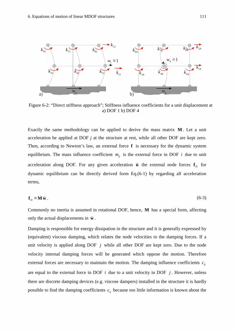
6. Equations of motion of linear MDOF structures
111
a)
11k
81k71k61k
51k41k31k
21k
b)
14k
24k
34k 44k 54k
64k 74k 84k
11 =w 14 =w
gw gw
Figure 6-2: “Direct stiffness approach”; Stiffness influence coefficients for a unit displacement at
a) DOF 1 b) DOF 4
Exactly the same methodology can be applied to derive the mass matrix M . Let a unit
acceleration be applied at DOF j at the structure at rest, while all other DOF are kept zero.
Then, according to Newton’s law, an external force f is necessary for the dynamic system
equilibrium. The mass influence coefficient ijm is the external force in DOF i due to unit
acceleration along DOF. For any given acceleration uɺɺ the external node forces Df for
dynamic equilibrium can be directly derived form Eq.( 6-1) by regarding all acceleration
terms,
wMf ɺɺ=D .
( 6-3)
Commonly no inertia is assumed in rotational DOF, hence, M has a special form, affecting
only the actual displacements in wɺɺ .
Damping is responsible for energy dissipation in the structure and it is generally expressed by
(equivalent) viscous damping, which relates the node velocities to the damping forces. If a
unit velocity is applied along DOF j while all other DOF are kept zero. Due to the node
velocity internal damping forces will be generated which oppose the motion. Therefore
external forces are necessary to maintain the motion. The damping influence coefficients ijc
are equal to the external force in DOF i due to a unit velocity in DOF j . However, unless
there are discrete damping devices (e.g. viscose dampers) installed in the structure it is hardly
possible to find the damping coefficients ijc because too little information is known about the

6. Equations of motion of linear MDOF structures
112
distributed damping process. Instead modal damping ratios, based on experience or
experimental data are utilised.
Working with larger structural elements, instead of a detailed finite element mesh, reduces the
degrees of freedom dramatically, resulting in a system of much smaller order, which of
course, is beneficial, but at the price of loosing information about the resulting stress
distribution. Nevertheless it can be recalculated by a static analysis using a more refined finite
element mesh. Unfortunately tall buildings consist of several thousand structural elements,
and further simplification might be necessary. It can be achieved by methods which are
described in the following sections.
6.4. Kinematic constraints
The introduction of kinematic constraints, which express the displacements of many degrees
of freedom in terms of a much smaller set of primary variables, is an uncomplicated method
to decrease the number of degrees of freedom further. Typically, the displacements of a group
of individual members, e.g. interstory columns, are constrained by the displacements of
floors. One of the most widely used applications of this type is the modelling of multiple-
story building frames1.
X
Y
Z
Figure 6-3: Twenty story building frame (2880 DOF)
Figure 6-3 shows a 20-story rectangular building frame with six frames (480 girders) parallel
to the X-Z-plane and 4 frames (400 girders) parallel to the Y-Z-plane. The total model

6. Equations of motion of linear MDOF structures
113
contains 480 columns, thus a total of 1360 one-dimensional elements. The number of nodes
interconnecting the elements is the same as the number of columns, yielding 2880 degrees of
freedom when allowing for three rotations and three translations per joint.
Taking the constraining effect of the floor slabs into consideration reduces this number
substantially, if each floor diaphragm is rigid in its own plane but flexible in the vertical
direction. These kinematic constraints reduce the degrees of freedom of each joint from six to
three. On top there is a rigid body motion in each floor yielding a total of
15002032/2880 =⋅+ degrees of freedom. Further reduction cannot be accomplished by
kinematic constraints, but e.g. the method of static condensation, can decrease the model size
further to about 2% of the original model, see e.g. Clough-Penzien1.
6.5. Static condensation
In contrast to the kinematic constraint idea the concept of static condensation is based on
static equilibrium constraints, and for a successful application of this technique the degrees of
freedom are divided into two types: those in which no mass or damping participates, denoted
by 0w and those who can develop inertia or damping forces, called Mw . Obviously this
approach assumes concentrated lumped masses which are found for most elements by simple
energy principles. Having recognised the different degrees of freedom, the equations of
motion under the effective loading TMeff ][ 0 fff = can be rearranged using “hypermatrices” as
indicated
=
+
+
MMMM f
f
w
w
KK
KK
w
w
C0
00
w
w
M0
00 00
2221
121100
ɺ
ɺ
ɺɺ
ɺɺ.
( 6-4)
Eq.( 6-4) can be solved for 01
11121
110 fKwKKw −− +−= M and back substitution yields the reduced
order dynamic system
( ) 0
1112112
1112122 fKKfwKKKKwCwM −− −=−++ MMMM ɺɺɺ .
( 6-5)
This static condensation procedure can be used to effectively reduce the degrees of freedom,
such as the reduction from 1500 to 60 in the building frame discussed in the previous section,
if all masses are lumped onto the floor level. The remaining 60 DOF correspond to the rigid
body motion of each floor. Up to this point, there was no major simplification, and all

6. Equations of motion of linear MDOF structures
114
dynamic systems generated with one method described above yield, independent of their
order, similar simulation results. Additional model reduction can only be achieved at the price
of a certain change in system dynamics. If, however, dominant degrees of freedom can be
located, further reduced models can be a good representation of the original system. Two
methods capable of such a simplification are the modal truncation, and a generalised order
reduction method appropriate to all linear, stable systems.
6.6. Modal truncation
A commonly used method in structural analysis is to perform dynamic investigations in the
modal space, and consequently restrict the research to the dominating mode-shapes. Several
well established methods have been developed for finding the mode vectors and solving the
vibration eigenproblem, most prominent amongst those are the Rayleigh-Ritz method and the
subspace iteration, see Clough-Penzien1. Instead of taking all modal coordinates and the
corresponding mode-shapes into account, only the major degrees of freedom are considered in
the investigation.
The main difficulty, however, is to determine the set of coordinates which depicts the
dynamic behaviour of the original system with sufficient precision, thus the key question is
which modal coordinates must be maintained to avoid significant modal truncation errors. To
evaluate the errors resulting from modal truncation, the dynamic response contributions of the
individual modes are considered. For an arbitrary mode i the equation of motion is given by
effiiiiii fqqq ,22 =++ ωωζ ɺɺɺ ,
( 6-6)
where the effective modal load factor is given by ( )( ) ( )ttwf effTigS
Tieffi fφfrMφ =+−= ɺɺ, , and
iφ denotes the i-th mode shape vector, normalised with respect to the modal mass,
ijjTi δ=Mφφ , see Eq.(1-37). By inspection of Eq.( 6-6) it can be concluded, that the relative
importance of single mode contributions to the total dynamic response depends on
• The modal load factor which depends on the interaction between mode shape and external
load.
• The spectrum of the applied external load.

6. Equations of motion of linear MDOF structures
115
• The dynamic magnification factor which depends on the ratio of the applied loading
frequencies to the modal frequency.
Assuming a time variant but spatially constant load distribution ( ) ( )tfteff rf = , a modal
participation factor exists, and is defined by rφTii =ξ , for derivations see Chapter 1. For any
ground motion of a single point excitation characterised by gwɺɺ , SrMr = and for simple cases
of high-rise framed structures with displacement degrees of freedom, Sr becomes
TS ]1,,1[ ⋯Mr = . Figures 6-4 a-c show typical flexural mode shapes of a high rise building,
and Figure 6-4d displays its mass distribution. Obviously the vector product STi rφ is relatively
large for the fundamental mode and is rapidly decreasing for higher mode shapes. For this
reason the participation factor of the first mode is dominant for ground excited structures. If
the load is not distributed uniformly, see e.g. Figure 6-4e for a force loading with common
time function, then the second mode has a large participation factor whereas the first and the
third mode would contribute only little to the overall response.
a) Mode 1 b) Mode 2 c) Mode 3 d) e)
tfteff rf =
Figure 6-4: a)- c) vibration mode shapes d)mass distribution e) locally distributed force loading with common time function
For a sufficiently long loading time, the dynamic magnification factor largely depends on the
excitation spectrum and the damping ratio of the modal equation. If the external loading
contains a resonant frequency, the corresponding mode shape is expected to cause important
contributions to the entire dynamic response.

6. Equations of motion of linear MDOF structures
116
Having identified the dominant modal coordinates, the modal truncation can be performed by
discarding all other coordinates. Often it is desired to perform this simplification without
loosing the physical interpretation of the original displacement coordinates. Let n denote the
order of the reduced system, then it is possible to describe the reduced order system with n
arbitrary elements of the original generalised displacement vector w . Firstly, the rows of the
matrix equation are rearranged by pre-multiplying with a transformation matrix T , such that
the coordinates which are kept are contained in the “observable” vector ow , whereas all
coordinates discarded form the vector rw . This rearrangement allows to give the equations of
motion of the structure under effective force loading by
efffwKwCwM =++ ɺɺɺ ,
TMM = , TCC = , TKK = ,
=
o
r
w
ww ,
= o
eff
reff
eff f
ff .
( 6-7)
M , C , K , w , efff denote the rearranged mass matrix, damping matrix, stiffness matrix,
displacement vector and excitation load vector, respectively. In modal coordinates Eq.( 6-7)
can be rewritten as
effTTTT fΦqΦKΦqΦCΦqΦMΦ =++ ɺɺɺ
( 6-8)
where
=
oo
rrT
M0
0MΦMΦ ,
=
oo
rrT
C0
0CΦCΦ ,
=
oo
rrT
K0
0KΦKΦ ,
=
ooor
rorr
ΦΦ
ΦΦΦ ,
=
o
r
q
=
=
o
r
ooor
rorr
o
r
q
q
ΦΦ
ΦΦ
w
ww .
( 6-9)
( 6-10)
( 6-11)
ooM , ooC , ooK , rrM , rrC , rrK denote the dominant modal mass, the dominant damping, the
dominant stiffness, the residual mass, the residual damping and the residual stiffness matrices,

6. Equations of motion of linear MDOF structures
117
respectively. All matrices are separated according to the dominant and residual modal
coordinates. The modal matrix Φ consists of the dominant (observable) mode-shape vectors
oiφ and the residual mode-shape vectors r
iφ :
],,,,,[ 11
onN
orn
r−= φφφφΦ ⋯⋯ .
( 6-12)
Through modal truncation the residual modes are neglected, 0q =r , and Eq.( 6-8) simplifies
to
reff
Tro
oeff
Tooooooooooo fΦfΦqKqCqM +=++ ɺɺɺ .
( 6-13)
From Eq.( 6-11) the relation between the modal coordinates and the displacement vector is
given by oooo qΦw = . Unless 0w contains only nodal points of a certain mode shape, the
inverse of ooΦ exists, and Eq.( 6-13) can be transformed to
reff
Tro
oeff
Tooooooooooooooooo fΦfΦwΦKwΦCwΦM +=++ −−− 111
ɺɺɺ .
( 6-14)
Eq.( 6-14) is very convenient because it still consists of a mass, damping and stiffness matrix,
and has the structure of a linear equation of motion, thus it can be handled with all tools
available for linear systems without any modifications. However, as a result of the order
reduction, the stiffness matrix might not be symmetric any more, thus TKK ≠ . If one is
interested in the discarded states rw Eq.( 6-11) has to be considered again and renders
ooorooror wΦΦqΦw 1−== .
( 6-15)
The method of strict truncation can be improved by a residualisation, where only dynamics of
the residual modes is neglected ( )0q0q == rr ɺɺɺ , , and Eq.( 6-8) simplifies to a static relation
which can be easily solved for rq :
( )reff
Trr
oeff
Torrrr fΦfΦKq += −1 .
( 6-16)
Inserting Eq.( 6-16) into Eq.( 6-11) renders a pseudo static component st0w
( )reff
Trr
oeff
Torrror
st fΦfΦKΦw += −10
( 6-17)

6. Equations of motion of linear MDOF structures
118
which must be added to the solution of Eq.( 6-14) for an improved accuracy.
6.7. Modal reduction
In the previous sections several different possibilities for the reduction of the number of
degrees of freedom in the dynamic system have been discussed. Static condensation, e.g. is
able to reduce the dynamic behaviour of a structural model to three independent motions per
floor. Further model reduction can be achieved by a modal transformation, and a subsequent
modal truncation, keeping only those mode-shapes which make major contributions to the
desired structural response quantities. Sometimes even the knowledge of participation factors
and dynamic magnification factors are insufficient to decide which modes to keep and which
to discard, and for this reason it is of importance to alternatively find a quantitative measure
reflecting the influence of certain state variables on the structural behaviour. The following
summary is based on a landmark paper by Moore2, where a state reduction method developed
for control engineering is presented. The key idea is to find a state transformation which gives
a clear indication which state variables contribute mainly to the structural response. These are
consequently dominating the system behaviour and must be kept, whereas all others are of
less importance and might be discarded. Such methods are of outmost importance in
automatic control since the order of the system model should be minimised for several
reasons, e.g. for controller design and implementation and for high sampling rates. It is
convenient to use a state space description of a system, Eq.(1-60),
auBzAz +=ɺ ,
zCy =
( 6-18)
with T],,,,,[ wvuwvuz ɺɺɺ= , A , B , C denoting the state space vector, the system matrix, the
input and output matrix, respectively. Depending on the excitation, the input term auB
represents either wind or earthquake loading. To be compatible with the nomenclature in
control literature, the system input vector is denoted au . No conflict of notation is to be
expected with the displacement of the fluid since it is hidden in the state vector z . The output
vector y describes the mechanical property of interest e.g. interstory drifts. At this point it is
necessary to assume that the structural dynamic system described by Eq.( 6-18) is controllable
and observable in a control engineering sense, see e.g. Müller3. However, this condition is

6. Equations of motion of linear MDOF structures
119
satisfied for most civil engineering problems. The first step in model reduction is to find the
influence of an input signal on the state variables. Among several possible measures, the
covariance matrix for an infinite time period
∫ dt
zzzzz
zzzzz
zzzzz
dt
nnn
n
n
TI
⌡
⌠
=⋅=
∞
∞
0
222212
222221
212121
0
⋯
⋮⋱⋮⋮
⋯
⋯
zzQ ,
( 6-19)
can be chosen (it converges for asymptotically stable systems). If it is possible to find a
transform BzTz = such that IQ becomes diagonal, then the diagonal elements are the
variances of the corresponding state. IQ depends on the input signal, and a unit impulse
excitation which contains the entire frequency spectrum, seems to be a suitable excitation.
The general solution of the dynamic system, Eq.( 6-18) is, see Eq.(1-66),
( ) ( ) ( ) ( ) ( )∫t
ta
ttt duetet0
00 τττ Bzz AA −− += ,
( 6-20)
where the matrix exponential is defined by Eq.(1-67). For a unit impulse input ( )00 == tu δ
and homogenous initial conditions, the system response simplifies to the Green’s function,
( ) Bz Atet = . Substitution into ( 6-19) renders an integral expression,
∫∞
=0
dtee tTtI
TAA BBQ ,
( 6-21)
which control engineers refer to as the controlability Gramian, see Moore2. If this matrix has
full rank, the system is controllable, in other words, any arbitrary state configuration can be
achieved by properly choosing the external input. As shown in Appendix B, IQ is equivalent
to the solution of the Lyapunov equation, see also Müller and Schiehlen3,4
0=++ TT
II BBAQQA .
( 6-22)
Having found a suitable expression describing the influence of a unit impulse on the state
variables, the influence of the state variables on the output y remains to be determined.
Similar to a performance index, the term

6. Equations of motion of linear MDOF structures
120
∫ ∫∞∞
==00
dtdtJ TTT zCCzyy
( 6-23)
characterises the effect of the state variables on the output. For free vibrations with arbitrary
initial conditions 0z , the properly reduced Eq.( 6-20) when substituted into Eq.( 6-23) yields
∫ 000
00 zPzzCCz AAI
TtTtT dteeJT
==∞
,
∫∞
=0
dtee tTtI
T AA CCP
( 6-24)
with the corresponding Lyapunov equation, see Appendix B,
0=++ T
IIT CCAPPA .
( 6-25)
In control literature, e.g. Müller3,4, IP of Eq.( 6-24) is commonly known as observability
Gramian. If this matrix has full rank, the system is called observeable, which means that any
state configuration can be reconstructed only by knowing the external input and output of the
dynamic system. Performing any regular state transformation T , Eq.( 6-18) becomes
uBzAz ˆˆˆˆ +=ɺ
zCy ˆˆ= ,
( 6-26)
where TATA 1ˆ −= , BTB 1ˆ −= , TCC =ˆ . Some little algebra renders the Gramians ( )TQ ,
( )TP after the transformation T as a function of the Gramians of the original system IQ and
IP :
( ) ∫ ( ) ∫ ( )TItTtTtTt dteedtee
TT 11
0
ˆˆ1
0
1 ˆˆ −−∞
−∞
− === TQTBBTBBTTQ AAAA ,
( ) ∫ ∫ TPTCCTCCTTP AAAAI
TtTttTtT dteedteeTT
===∞∞
0
ˆˆ
0
ˆˆ .
( 6-27)
If it is possible to find a transformation to generate an often called balanced system, such that
( ) ( ) ),( 22
21 ndiag σσ ⋯== TQTP , n221 σσσ >>> ⋯ , then 2
iσ describes the effect of a unit
impulse on the state as well as the relation of this state on the system response. In other
words: if 11 <<σσ i then this state has little influence on the overall dynamic behaviour and

6. Equations of motion of linear MDOF structures
121
might be neglected. Moore2 has shown, that such a transformation can be found in two steps:
Firstly, both symmetric matrices IP and IQ are decomposed into TPPPI VΣVP 2= and
TQQQI VΣVP 2= with QV , PV denoting unitary matrices ( 1−= VVT ) and 2
PΣ , 2QΣ represent the
diagonal singular value matrices, see e.g. Skogestad5. A first state transformation
QQΣVT =1 ,
( 6-28)
can be used to generate an input-normal-system with ( ) IQTQ T ==11 , where I denotes the
identity matrix, and ( ) QQITQ
TQ ΣVPVΣPTP T ==
11 . A subsequent modal decomposition of the
transformed system renders a new set of matrices
IQT =
1,
TPPP
1
2
111 TTTT VΣVP =
( 6-29)
From Eq.( 6-29), it is quite obvious that there exists a second transformation 2T to bring both,
1TP and 1TQ to diagonal form. By substitution, it can be proven that for the second state
transformation the transformation matrix
21
112
−=TPTP ΣVT ,
( 6-30)
must be applied in order to obtain the balanced state representation where
( ) bal
T
balIbalbal ΣTQTQ == −− 11 ,
balbalITbalbal ΣTPTP == ,
21 TTT =bal , ( )11 TPTΣ IT
bal σ= .
( 6-31)
( 6-32)
( 6-33)
( )11 TPT ITσ denotes the diagonal matrix containing the singular values of 11 TPT I
T . Now,
balQ and balP are two identical diagonal matrices whose diagonal elements 2iσ determine
significance of the i-th states on the dynamic response. It is important to mention that the
individual components 2iσ of the balanced system might not differ a lot. In such a situation no
system state can be removed without a deterioration of the model’s quality. However, if small

6. Equations of motion of linear MDOF structures
122
values of 2iσ exist, then the corresponding state can be neglected and consequently removed
by either truncation or residualisation. With appropriate partitioning, the state vector is given
by T]ˆ,ˆ[ˆ 21 zzz = , where 1z should be removed, and Eq.( 6-18) can be rewritten as
auBzAzAz 12121111ˆˆˆˆˆˆ ++=ɺ ,
auBzAzAz 22221212ˆˆˆˆˆˆ ++=ɺ ,
2211 ˆˆˆˆ zCzCy += .
( 6-34)
In truncation the first set of equations in Eqs.( 6-34) is simply removed and 0z =1ˆ , as in
modal truncation. Residualisation, on the other side is similar to static condensation, where
instead of discarding all states associated with 1z , the time derivative is simply set to zero
0ˆ1 =zɺ . One can then solve for 1z in terms of 2z and u and back substitution gives
( ) ( ) auBAABzAAAAz 11
112122121
1121222ˆˆˆˆˆˆˆˆˆˆ −− −+−=ɺ
( ) auBACzAACCy 11
1112121
1112ˆˆˆˆˆˆ −− −−=
( 6-35)
Furthermore attention has to be drawn to the fact that the successful application of model
reduction is largely dependent on the structural response quantities included in the possible
output vector y . A warning example is a simple untuned mass absorber system where the
order reduction potential depends on the response one is interested in, e.g., the main mass
displacement or the absorber displacement. For exactly the same system the former situation
will allow a successful order reduction whereas in the latter case no reduction is feasible. For
this reason the elimination of states is generally difficult unless the output quantities have
been determined.
6.8. Examples
Several methods discussed within this chapter have been successfully applied to real civil
engineering problems, presented in Chapter 9, where high-rise buildings are investigated.
Several benchmark structures have been published by Spencer6,7 where the reduction of the

6. Equations of motion of linear MDOF structures
123
degrees of freedom is shown in detail: first the complex structures are discretised by finite
elements, usually frames, and a model with several thousand degrees of freedom is obtained.
The use of kinematic constraints and static condensation reduce the model to several hundred
degrees of freedom. A further reduction can be achieved by modal approximations or
balanced realisations. Investigations will show that most buildings have a high reduction
potential. Depending on the excitation, the final model can be reduced by a factor of up to
100-1000.
6.9. References
1 Clough, R.W., Penzien, J., Dynamics of Structures, McGraw-Hill, Singapore, 2nd edition,1993 2 Moore, B.C, Principal Component Analysis in Linear Systems: Controllability, Observability, and Model
Reduction, IEEE Transaction on Automatic Control, Vol. AC26(1), pp.17-32, 1981 3 Müller, P.C., Stabilität und Matrizen, Springer-Verlag, 1977 4 Müller, P.C., Schiehlen, W.O., Lineare Schwingungen, Akademische Verlagsgesellschaft, Wiesbaden, 1976 5 Skogestad, S., Postlethwaite, I., Multivariable Feedback Control, John Wiley & Sons, Chichester, GB, 1988 6 Spencer, B.F. Jr., Dyke, S.J., Doeskar, H.S., Part I: Active Mass Driver System, Part II: Active Tendon System,
Special issue of Earthquake Engineering and Structural Dynamics, vol.27(11), pp.1127-1148, 1998 7 Spencer, B.F. Jr., Christenson, R. Dyke, S.J., Next Generation Benchmark Problem, Proceedings of the Second
World Conference on Structural Control, (ed. Nishitani, A..), Kyoto, Japan, 1998, also www-publication:
http://www.nd.edu/~quake/

7. Optimisation of multiple TLCDs and MDOF structural systems in the state space domain
124
7. Optimisation of multiple TLCDs and MDOF structural systems in the
state space domain
Traditionally, dynamic systems have been described by second order differential systems
because Newton’s law as well as energy principles (e.g. Lagrange equations of motion,
Hamilton’s principle) render inertia proportional to acceleration. Alternatively, the state space
representation can be used to describe dynamic systems, and it turns out that it is particularly
suitable for dynamic investigations, since the difference between non-classically and
classically damped systems vanish, the design and incorporation of the absorber into the
structural model is straightforward, and numerical processing is possible. A structural model
with dozens of degrees of freedom can be quite difficult to investigate, and intuitive analytical
design schemes must give way to a more systematic approach, which is adaptable for
automated processing. Independent of the size of the structural model, any linear structure
with N degrees of freedom can be described by, see Eq.(6-1), which is properly generalised
to include a number of n TLCDs installed in the building,
( ) AgS tw fLfrMwKwCwM ++−=++ ɺɺɺɺɺ
( 7-1)
where Af , L denote the structure-absorber interaction forces and a position matrix,
respectively. The TLCD position matrix has the following form:
TLCDbyinfluencediswhichfreedomofdegree
TLCDofnumber
001
010 ←
↑
=⋯
⋮⋱⋮⋮
⋯
L
( 7-2)
Obviously L is a sparse matrix of dimension [ ]nN × . The components of [ ]TnA ff ,,1 ⋯=f
are the individual interaction forces if of the TLCDs, given by Eq.(4-31) or Eq.(4-60),
][ ,, iiabsifi uwmf ɺɺɺɺ κ+−= ,
( 7-3)
where ifm , , iabsw ,ɺɺ represents the liquid mass of the i-th TLCD and the absolute acceleration
of its supporting floor. The corresponding TLCD equation of motion is, see Eq.(4-11),

7. Optimisation of multiple TLCDs and MDOF structural systems in the state space domain
125
iabsiiiiiii wuuu ,22 ɺɺɺɺɺ κωωζ −=++ ,
( 7-4)
It has to be pointed out that the following derivation is only valid for the case where w
describes the floor displacement with respect to the basement. If the vector w contains e.g.
interstory drifts, a linear transformation wTw =b to displacement coordinates bw (with
respect to the base) is inevitable for the calculation of the interaction forces. For convenience,
the TLCDs dynamics, given by Eqs.( 7-3) and ( 7-4), can be formulated in matrix notation:
( )[ ]uiwTLMf ɺɺɺɺɺɺ K++−= gT
AA w ,
( )g
TAA wɺɺɺɺɺɺɺ iwTLuKuCu +−=++ K ,
( 7-5)
( 7-6)
where
( )nffA mmdiag ,1, ,⋯=M , ( )nniA diag ωζωζ 2,,2 1 ⋯=C
( )221 ,, nA diag ωω ⋯=K ,
( )ndiag κκ ,,1 ⋯=K , ( )ndiag κκ ,,1 ⋯=K
( 7-7)
Eliminating the interaction forces in the structural equations by substituting Eq.( 7-6) into
Eq.( 7-1) generates the coupled matrix equations of motion:
( )
+
+−
=
+
+
+
0
f
i
iMLrM
u
w
K0
0K
u
w
C0
0C
u
w
ITL
MLTLMLM
twg
AS
AAT
AT
A
ɺɺ
ɺ
ɺ
ɺɺ
ɺɺ
K
K
K
( 7-8)
An explicit expression for the building and absorber accelerations wɺɺ ,uɺɺ can be obtained by
firstly defining the regular non-diagonal mass matrix of the combined system
+=
ITL
MLTLMLMM T
AT
AS
K
K,
( 7-9)
and, secondly, pre-multiplying Eq.( 7-8) with its inverse

7. Optimisation of multiple TLCDs and MDOF structural systems in the state space domain
126
( ).1
111
+
+−
−
−=
−
−−−
0
fM
i
iMLrMM
u
w
K0
0KM
u
w
C0
0CM
u
w
t
w
S
gAS
SA
SA
S ɺɺɺ
ɺ
ɺɺ
ɺɺ
K
( 7-10)
This system of second order differential equations can be converted to a first order state space
representation by introducing the new state vector [ ]TTTTT uwuwz ɺɺ= , and its time derivative
( ) ( )tw fgg fEezRBAz +−+= ɺɺɺ ,
( 7-11)
where in a hypermatrix notation
−
−
=−−
00
0CM
00
0KM
I0
0I
00
00
A11
SS
,
−
−
=−−
I0
0IM
I0
0IM
00
00
00
00
B11
SS
,
=
A
A
C000
0000
00K0
0000
R ,
+=
−
i
iMLrMM
0
0
e
K
ASS
g
1
,
=
−
0
IM
0
0
E1
S
f .
( 7-12)
A system matrix RBAA +=r apparent in Eq.( 7-12) can be used, however sometimes the
separated two term expression BRA + has the advantage that A solely contains the given
structural dynamics and the second term, RB includes the TLCD design parameter, natural
frequency and damping ratio.
7.1. Optimisation for free vibration of MDOF structure with several TLCD
installed
Having established the set of ( )nN +2 equations of motion, the dynamic performance of the
system has to be determined, often by a performance index, which is a scalar measure of the
system behaviour. The choice of a practical performance index is difficult and becomes a
critical task where the engineer’s knowledge and experience plays a central role. Usually,
deep insight into the structural behaviour, and a good understanding of dynamic phenomena
are required to be able to describe a complex behaviour by a simple number. A commonly

7. Optimisation of multiple TLCDs and MDOF structural systems in the state space domain
127
used technique is to examine the free vibrations of a building with the aim of minimising the
time integral of a weighted sum of the quadratic state variables for the infinite time interval
∞<≤ t0 . Mathematically this quadratic performance index is described by
( ) ( )∫∞
=0
τττ dJ T zSz ,
( 7-13)
with a symmetric, positive semidefinite weighing matrix S , which defines the relative
importance of the states with respect to each other. The performance index given in Eq.( 7-13)
quantifies the free vibration such, that large displacements and velocities are rated heavily - an
important criteria from a practical point of view. However, the initial conditions and the
weighing matrix S must be chosen to account for engineering requirements. Furthermore it is
important to know efficient algorithms for the computation of J , as its minimisation is, in
general, performed numerically. For given initial conditions ( ) 00 zz = the free vibration is
given by ( ) 0zetz tAr= . Inserting into ( 7-13) yields
∫ 00
0 zSz AA∞
= τττ deeJ rTrT .
( 7-14)
Integration by parts can solve this integral expression, see Appendix B, and the quadratic
performance index for an infinite time interval simplifies to
00 zPzTJ = ,
0=++ SPAPA rTr ,
( 7-15)
where P is the solution of an algebraic Lyapunov matrix equation. Consequently, the
calculation of the quadratic performance index J has been reduced to the computation of the
solution P of a linear matrix equation. For asymptotically stable systems, P has a unique
solution if S is positive semidefinite, see e.g. Müller1. Finding the solution of a Lyapunov
equation is a standard problem in numerical mathematics, and powerful algorithms are readily
available, see e.g. Control Toolbox of Matlab5.
After J has been defined, it is possible to compute the free system parameters, as defined by
the nonzero diagonal elements of R , see Eq.( 7-12). The latter must be varied in order to
optimise the free vibrations according to Eq.( 7-14). Optimal parameter are found when J
reaches a minimum or equivalently

7. Optimisation of multiple TLCDs and MDOF structural systems in the state space domain
128
0=∂∂
RJ
.
( 7-16)
Unfortunately, an analytical expression for Eq.( 7-16) can hardly be found, and some of the
parameters can have range limitations ( 0>Aζ , maxmin ωωω << A ) so that the optimisation is
often performed numerically.
Yet, the choice of the initial condition is still not discussed. Basically, 0z can take any value,
but the response due to a unit impulse load is meaningful from an engineering perspective.
For homogenous initial conditions and ground excitation, this response is given by Eq.(1-66),
( ) gtret ez A= . Therefore a suitable choice of 0z would be gez =0 . Furthermore, the weighing
function S has to be selected such, that the performance index reflects important physical
quantities. If displacements or velocities are contained in J , then S will be of diagonal shape.
Alternatively, the minimisation of the accumulated structural energy would be a meaningful
performance index. If the instantaneous structural energy 2)( wMwwKw ɺɺTT
instE += is
defined as the sum of the relative kinetic and strain energy, then
zSzT
instE = ,
=
0000
0M00
0000
000K
S ,
=
u
w
u
w
z
ɺ
ɺ,
( 7-17)
and the performance index represents the accumulated energy, which is minimised for free
vibrations.
The optimisation for free vibration guarantees optimal behaviour if there is a certain state
disturbance at 0=t . As the performance index is solely defined in the time domain, the free
vibration optimisation method must be categorised as a time domain method. However, as an
impulse load is rarely applied to a building, a more realistic design methodology which
attenuates external excitation defined in the frequency domain is discussed next.

7. Optimisation of multiple TLCDs and MDOF structural systems in the state space domain
129
7.2. Frequency response optimisation for MDOF structures with several
TLCD installed
The frequency response spectrum, in particular the amplitude response curve, is a quantity of
major importance for describing the sensitivity to external disturbances in the frequency
domain. A typical example of a frequency domain method is the optimisation according to
DenHartog, see Section 2.6.2, where the maximal amplitude magnification is reduced to
obtain a “disturbance rejecting” behaviour. In structural dynamics, resonance problems are
often tackled by the application of dynamic vibration absorbers. Therefore the frequency
response shaping should be focused at the critical frequency range, as well as by taking the
excitation spectrum into account.
7.2.1. Determination of a performance index in the frequency domain
Since the amplitude response function ( )νA and the Fourier transformed of the impulse
response function ( )νh are proportional and related by a constant scaling factor χ ,
( ) ( )νχν hA S= , a mathematical generalisation of the DenHartog performance criterion for
SDOF systems can be stated by
( ) minimummax →
Ω∈= ν
νhJ , maxmin νν ≤Ω≤ ,
( 7-18)
where Ω denotes the frequency range of interest. For multiple degree of freedom systems
many impulse response functions can be defined, e.g. ( ) ( )νν Nhh ,,1 ⋯ which must be
minimised simultaneously. In such a situation, Eq.( 7-18) can be extended to
( ) ( ) minimum,,max 11 →
Ω∈= νν
νNN hshsJ ⋯ , maxmin νν ≤Ω≤ ,
( 7-19)
where the positive weighing factors 0>is are introduced to describe the importance of the
different states. A generalisation which takes into account frequency dependent weighing
factors ( )νis is commonly referred to as ∞H design, see e.g. Levine2, Müller3 and Ludyk4.
However, the calculation of the ∞H norm, defined by ( ) ( )( )kk
kdhh ∫
∞
∞→∞ =0
lim ννν , is based
on an iterative method, and thus quite time consuming. Nevertheless, efficient algorithms are
available in numerical toolboxes, e.g. Control Toolbox of MATLAB5.
A second method of measuring the disturbance attenuation is to minimise the area below the
impulse response curve of a SDOF system,

7. Optimisation of multiple TLCDs and MDOF structural systems in the state space domain
130
( )∫ →=max
min
minimum2
ν
ν
νν dhJ .
( 7-20)
Again, a quadratic description is chosen to penalise high amplifications. If several impulse
response functions are of interest, e.g. in case of a MDOF-system, an extension of Eq.( 7-20)
can be given straightforwardly
( ) ( ) minimum1
2max
min
→=∑ ∫=
N
iii dhsJ
ν
ν
ννν ,
( 7-21)
where is is a weighing factor which is introduced to account for the different significance of
the state variables. Obviously, dominant resonant peaks increase the performance measure J
drastically and as a result the optimisation according to Eq.( 7-21) will reduce those peaks
noticeably, leading to similar results as an optimisation according to Eq.( 7-19). This reduction
can be explained by the fact that vibration prone structures have only small damping ratios
and the amplitude magnification at the critical resonant frequency causes a major contribution
to the performance index.
The first step to evaluate Eq.( 7-21) is to substitute the quadratic amplitude magnification by
( ) ( ) ( )ννν hhh ⋅= *2 where * denotes the conjugate complex of a number. Then J simplifies
to
( ) ( ) ( )∫=max
min
ν
ν
νννν dJ H hSh ,
( 7-22)
where ( )νh is given by Eq.(1-68). The superscript H denotes the complex transposed of a
matrix, and ( )νS is a positive semidefinite, frequency dependent weighing matrix, composed
of the weighing factors ( )νis . For the special case of an unlimited frequency range
−∞=minν , +∞=maxν and a constant weighing matrix S , Eq.( 7-22) can be rewritten as
( )∫ ∫∞
∞−
∞
∞−
−= νν ddtetJ tiH hSh ,
( 7-23)

7. Optimisation of multiple TLCDs and MDOF structural systems in the state space domain
131
where ( )νh is replaced by its corresponding inverse Fourier transformed time function ( )th .
Since, for stable systems the integral expressions converge, it is legitimate to rearrange the
integral expressions to obtain
( ) ( ) ( ) ( )∫∫ ∫∞
∞−
∞
∞−
−∞
∞−
== dtttdttdeJ TtiH hShhSh πνν ν 2 ,
( 7-24)
where the time reversal property of the Fourier transform was used ( )( ) ( )thh ** =−ν-1F , see
e.g. Levine2 and Lüke6. The impulse response function vanishes for 0<t , the lower
integration limit can thus be changed to zero. From the general solution of linear differential
equations, see Eq.(1-65) it follows directly that, for homogenous initial conditions, the
impulse response function ( )th becomes
( ) ( )∫ ( ) ( ) gt
t
gretdtt ebΓeΓh A==−= ττδτ
0
,
( 7-25)
assuming homogenous initial conditions. Thus
gTg deeJ r
Tr eSe AA
∫∞
∞−
= νπ ττ2 ,
( 7-26)
where the excitation vector ge , Eq.( 7-12), is assumed to be constant, and the system matrix
A must be asymptotically stable. Further simplification is possible because the integral
expression in Eq.( 7-26) is again the solution of the Lyapunov matrix equation, and the
frequency dependent optimisation index simplifies to, see e.g. Müller-Schiehlen7, p.249,
ggJ ePeπ2= ,
0=++ SAPPA rTr ,
( 7-27)
In fact the optimisation of the quadratic amplitude response function for an unlimited
frequency range yields exactly the same result as the optimisation of the free vibration if the
initial condition is chosen to be gez π20 = , which corresponds to a scaled unit impulse
excitation. This result is not surprising and states that under the given conditions both
optimisation methods yield the same TLCD tuning parameter, as the spectrum of a unit
impulse is considered as a unit intensity white noise signal. If coloured noise excitations are

7. Optimisation of multiple TLCDs and MDOF structural systems in the state space domain
132
investigated, the same optimisation idea can be used, but an additional filter function must be
included in the dynamic system, for such alternatives, see subsequent Section 7.5
7.3. Stochastic optimisation: Minimum Variance
The optimisation methods presented so far, did not take the random character of wind or
earthquake loading into account. Excitation forces generated by a random process cause the
dynamic response to be a random process as well. For linear systems and simple random
excitation processes it is possible to calculate stochastic response quantities like the state
variances. Well written introductions into random vibrations can, e.g. be found in Lin8,
Newland9, Parkus10, Wirschig11, Yang12, amongst others. For any continuous ergodic (hence
stationary) time process X , characterised by its probability density ( )xp , the expectation
value is given by
[ ] ( )∫T
T
dttxT
XE−
=2
1,
( 7-28)
but for vibrations the expectation value vanishes [ ] 0=XE , and thus the autocorrelation
function ( )τR becomes the most important response quantity. For the stationary process it is
defined by
( ) ( ) ( )[ ]ττ += txtxER ,
( 7-29)
and its Fourier transform, ( )ωxS , is called the spectral density function of X . The variance
of a function in time domain is given by
( ) ( ) ( )0]][[ 222 RtxEtxE =−=σ .
( 7-30)
For a single output ( )ty of a linear system excited by an external excitation ( )twgɺɺ , the
autocorrelation function is given by
( ) ( ) ( )[ ] ( ) ( )∫ ( ) ( )∫
−+⋅−=+=∞
∞−
∞
∞−222111 τττττττττ dtwhdtwhEtytyER gg ɺɺɺɺ ,
( 7-31)

7. Optimisation of multiple TLCDs and MDOF structural systems in the state space domain
133
where ( )τh denotes the scalar impulse response function. For a stable system both integral
expressions converge, and it is allowed to replace the two separate integrals by a single
double integral. Computation of the expectation in Eq.( 7-31), and rearrangement of the
integrals yields, see e.g. Newland9 and Parkus10
( ) ( ) ( ) ( ) ( )[ ]
( ) ( ) ( )∫ ∫
∫ ∫∞
∞−
∞
∞−
∞
∞−
∞
∞−
−+=
−−+=
212121
211221
τττττττ
ττττττττ
ddRhh
ddtwtwEhhR
gw
gg
ɺɺ
ɺɺɺɺ
( 7-32)
where gwR ɺɺ denotes the autocorrelation function for the excitation forces, see Eq.( 7-29). This
involved expression can be considerably simplified as follows. A Fourier transformation of
gwR ɺɺ into its frequency domain counterpart gwSɺɺ
and substitution into Eq.( 7-32) yields
( ) ( ) ( ) ( ) ( )∫ ∫ ∫∞
∞−
∞
∞−
−∞
∞−
−+= ωττωττπ
τ τττω dddSehhRgw
j2121
21
2
1ɺɺ .
( 7-33)
Rearrangement of the integral expressions, followed by another Fourier transformation
renders a simpler and very useful expression for ( )τR :
( ) ( ) ( ) ( ) ( )∫∫∞
∞−
∞
∞−
== ωωπ
ωωωωπ
τ τωτω deSdeShhR jy
jwg 2
1
2
1 *ɺɺ ,
( ) ( ) ( ) ( )ωωωωgwy ShhSɺɺ
*= , ( ) ( )∫∞
∞−
= ττω τω dehh j* , ( ) ( ) ττω τω dehh j
∫∞
∞−
−=
( 7-34)
where the time reversal property of the Fourier transform was applied in the definition of *h ,
and ( )ωyS denotes the power spectral density of the system’s response. The calculation of the
variance yσ is a special case of the autocorrelation function and thus obtained by setting
0=τ in Eq. ( 7-34), see e.g. Lin8, Newland9, Parkus10, Wirschig11, Spanos13,
( ) ( ) ( ) ( ) ωωωωπ
σ dShhRgwy ∫
∞
∞−
== ɺɺ
*2
2
10 .
( 7-35)

7. Optimisation of multiple TLCDs and MDOF structural systems in the state space domain
134
For linear systems with G inputs ( )twiɺɺ the corresponding expression for Eq.( 7-35) can be
given by
( ) ( ) ( ) ( ) ωωωωπ
σ dShhRG
r
G
swwsry
sr∫ ∑∑∞
∞− = ===
1 1,
*2
2
10
ɺɺɺɺ,
( 7-36)
where ( )thi represents the impulse response function due to an excitation at the i-th input. The
cross spectral density sr wwS ɺɺɺɺ , is defined as the Fourier transform , sr wwR ɺɺɺɺF of the cross
correlation ( ) ( ) ( )[ ]ττ += twtwER srww srɺɺɺɺ
ɺɺɺɺ , . If the system of interest has multiple inputs and
outputs the extension of Eq.( 7-36) can be given conveniently in matrix notation
( ) ( ) ( ) ωωωωπ
dH∫∞
∞−
= HSHΣ2
12 ,
( 7-37)
where S , H denote the matrix of spectral densities and the matrix of complex impulse
response functions, respectively. For physical white noise broad band excitation, const=S ,
Eq.( 7-37) can be simplified further by replacing ( )ωH by its inverse Fourier transformed time
function ( )tH ,
( ) ( )∫∞
∞−
= dttt THSHΣ2 ,
( 7-38)
where the time reversal property of the Fourier transform was applied again,
( )( ) ( )thh ijij** =−ν-1
F . Since ( ) EH A tret = , where E denotes the excitation input matrix given
by e.g. Eq.( 7-12), fEE = or ],,[ ,1, Ggg eeE ⋯= , Eq.( 7-38) simplifies further
∫∞
∞−
= dtee tTt Trr AA ESEΣ
2 ,
( 7-39)
The integral expression of Eq.( 7-39) is the solution of a Lyapunov equation, and thus the
variances are given by, see e.g. Müller-Schiehlen7, p.269,
0ESEAΣΣA =++ TTrr
22 .
( 7-40)

7. Optimisation of multiple TLCDs and MDOF structural systems in the state space domain
135
7.4. Comments on systems with multiple inputs
If one is dealing with a multiple input system the performance index has to be modified. For
the statistical variance optimisation an analytical solution can be obtained, which is given by
Eq.( 7-37). If the excitation inputs are independent variables then the cross spectral densities
vanish, and the SRSS (square root of sum of squares) rule for the standard deviation yσ
yields the exact solution, see e.g. Newland9
( ) ( ) ( ) ∑∑ ∫==
∞
∞−
==N
ssy
N
sfssy dSHHs
1
2,
1
*2 σωωωωσ ,
∑=
=N
ssyy
1
2,σσ ,
( 7-41)
where 2,syσ denotes the variance of output y due to the s-th input force sf . As the other
optimisation methods presented above are more of an intuitive character, there is no direct
procedure available to derive a mathematical description for several inputs. From an
engineering point of view the SRSS method seems to be most suitable, although other criteria
like simple summation or weighted summation of the single source excitation indices are
possible.
7.5. Coloured noise input
All optimisation methods presented so far have assumed stationary random, physical white
noise excitation X , mathematically defined uncorrelated
( ) ( )τδτ 0SRx = ,
( 7-42)
where 0S and ( )τδ denote the white noise intensity and the Dirac delta function of the
uncorrelated process. Although any real excitation process can hardly be described by white
noise excitation, it helps to overcome several mathematical difficulties, and allows to obtain
quite general and simple results. A more practical direct generalisation of the white noise

7. Optimisation of multiple TLCDs and MDOF structural systems in the state space domain
136
process is given by the coloured noise process, which is defined as the output of a dynamic
shape filter for a white noise input. Figure 7-1 shows the spectral density of a white noise
process and the coloured noise output of an arbitrary dynamic filter, which must be chosen to
approximate a real measured process, by the output of the filter due to a white noise input
signal.
circular frequency ν
0 20 40 60 80 100
pow
er s
pect
ral d
ensi
ty [d
B]
-40
-30
-20
-10
0
10
20
white noisecolored noise
Figure 7-1: Spectral density of white noise input signal and a coloured noise output signal
All linear dynamic filters of order ΨN can be described in state space formulation as
ξψψ BψAψ +=ɺ
ξψψ DψCψ +=
( 7-43)
where ξ , Ψ are a scalar or vector physical white noise input and the matching scalar or
vector coloured noise output, respectively. If the excitation process, the solution of Eq.( 7-43),
is applied to a structural system of order N , given by Eq.( 7-11), then the resulting system
dynamics becomes
ξBzAz +=ɺ ,
=
ψ
ψ
A0
CEAA ,
=
ψ
ψ
B
DEB
( 7-44)

7. Optimisation of multiple TLCDs and MDOF structural systems in the state space domain
137
Note that the new system, given by Eq.( 7-44), is again a linear system, but with an extended
system order of Ψ+ NN .
In earthquake engineering only lowpass filter are of interest, and soil amplification is often
modelled with the Kanai/Tajimi, a typical second order filtering function, see Clough-
Penzien15 or Shinozuka14, which is given by
( ) ( ) ( )ωξωωξ 11 H= , ( ) ( )( )( ) ( )11
21
111
21
21
ΨΨΨ
ΨΨ
+−
+=ωωζωω
ωωζωi
iH ,
( ) ( ) ( )ωξωωξ 122 H= , ( ) ( )( )( ) ( )22
22
22
2
21 ΨΨΨ
Ψ
+−=
ωωζωω
ωωωi
H .
( 7-45)
( 7-46)
Eq.( 7-45) defines a low-pass filter function which amplifies the frequency content in the
neighbourhood of 1Ψ= ωω and attenuates the frequency content for 1Ψ> ωω with 40dB per
decade. The second filter equation, Eq.( 7-46), attenuates the frequencies below 2Ψ< ωω . The
parameters 1Ψω and 1Ψζ must be adapted to local soil conditions. 2Ψω and 2Ψζ can be
adapted to produce the desired filtering of the very low frequencies. Assuming a physical
white noise excitation, and putting the filtering equations in series generates the complete
filter dynamics:
( ) ( ) ( ) ( )ωξωωωξ 212 HH= ,
( 7-47)
The spectral density of 2ξ is given by
( ) ( )( )( )( )( ) ( ) ( )( ) ( )
02
22
2
22
2
2
12
1
22
1
22
21
21
4141
41SS
−−
−−
+=
ΨΨΨΨΨΨ
ΨΨΨΨ
ωωζωωωωζωω
ωωωωζω ,
( 7-48)
where 0S describes the intensity of the physical white noise input. In Clough-Penzien15 the
above given Eqs. ( 7-45)-( 7-48) are applied to generate artificial earthquake ground motions.
To account for the limited time of strong motion, the artificially generated physical white
noise input is additionally multiplied with an envelope function. For the implementation of
box-type or exponential envelope functions see Ziegler16 or Höllinger17, where Priestley’s
formula was adapted for nonstationary random excitation. The power spectral density
( ) ( ) 01 SHSgg ⋅= ωω of the ground acceleration in Kanai-Tajimi representation, Eq.( 7-45), as

7. Optimisation of multiple TLCDs and MDOF structural systems in the state space domain
138
a function of ω , srad201 =Ψω 8.01 =Ψζ , 3240 10260 smS −⋅= , is given in Figure 7-2,
see Hasenzagl et al.18
Figure 7-2: Power spectral density ( ) ( ) 01 SHSgg ⋅= ωω of the ground acceleration in Kanai-
Tajimi representation as a function of ω , srad201 =Ψω 8.01 =Ψζ , 3240 10260 smS −⋅= , see
Hasenzagl et al.18
7.6. Remarks on the numerical optimisation and choice of initial
conditions
A common problem of numerical optimisation is the fact that most algorithms, e.g. all
gradient methods, terminate in a local minimum, instead of finding the global minimum. The
success of the numerical optimisation sometimes depends on the initial values (good
estimates) for the design parameters. Several simulations have shown that the understanding
of absorber dynamics helps when choosing the initial TLCD configuration. It is possible to
find the global minimum after some trials. As a general rule, every TLCD should be used to
reduce one single resonance only, and thus the initial natural TLCD-frequency can coincide
with the structural resonant frequency. This rule of thumb is also valid, if several TLCDs are
dedicated to a single resonant frequency. The choice of the position in the building is mainly
determined by the structural mode shapes. The larger the modal displacements at a certain
floor, the better the performance of the absorber, as discussed in Chapter 5. Once the initial
configuration is found an optimisation using a gradient method quickly finds an optimal
TLCD parameter design. According to the above given rule several other TLCD

7. Optimisation of multiple TLCDs and MDOF structural systems in the state space domain
139
configurations can be tested, and the optimal parameters can be quickly determined. For the
optimisation itself standard numerical algorithms are applied, e.g. Matlab19.
7.7. References
1 Müller, P.C., Stabilität und Matrizen, Springer Verlag Berlin, 1977 2 Levine, W.S, (editor), The Control Handbook, CRC Press 1995 3 Müller, K., Entwurf robuster Regelungen, Teubner Stuttgart, 1996 4 Ludyk, G., Theoretische Regelungstechnik 2, Springer Lehrbuch, 1995 5 MATLAB, User Guide, Control Toolbox, MathWorks Inc., Version 5.3.1, 1984-2001 6 Lüke, H.D., Signalübertragung, Springer, 6th edition, 1995 7 Müller, P.C., Schiehlen, W.O., Lineare Schwingungen, Akademische Verlagsgesellschaft, Wiesbaden 1976 8 Lin, Y.K., Cai, G.Q., Probabilistic Structural Dynamics, McGraw-HIll, 1995 9 Newland, D.E., An Introduction into Random Vibrations, Spectral & Wavelet Analysis, 3rd ed.,Longman
Scientific and Technical, 1993 10 Parkus, H., Random Processes is Mechanical Sciences, CISM Courses and Lectures, Springer Verlag, 1969 11 Wirschig P.H., Paez, T.L., Orith, K., Random Vibrations, John Wiley 1995 12 Yang, C.Y., Random Vibrations of Structures, John Wiley 1986 13 Spanos, P.D., Random Vibration and Statistical Linearisation, John Wiley & Sons, 1990 14 Shinozuka, M., Schueller, G.I., Stochastic Methods in Structural Dynamics, Martinus Nijhoff Publishers, 1987 15 Clough, R.W., Penzien, J., Dynamics of Structures, 2nd ed., McGraw-Hill, New York, 1993 16 Ziegler, F., Random Vibrations: A spectral method for linear and nonlinear structures, Probabilistic Eng.
Mech., vol.2(2), 1987 17 Höllinger, F., Ziegler, F., Instationäre Zufallsschwingungen einer elastischen Gewichtsmauer bei beliebig
geformtem Becken, ZAMM, vol.63, pp.49-54, 1983 18 Hasenzagl, R., Irschik, H., Ziegler, F., Design Charts for Random Vibrations of Elasto-plastic Oscillators
Subjected to Kanai-Tajimi Spectra, Reliability Engineering and System Safety, vol.23, pp.109-126, 1988 19 MATLAB, User Guide, Optimisation Toolbox, MathWorks Inc., 1984-2001

8. Active devices for vibration damping
140
8. Active devices for vibration damping
The permanent research and investigation of structural dynamics in the last decades has
resulted in the development of active structural control systems, which are a logical advance
of passive systems with the innovative idea of injecting energy in the structural system to
improve the dynamic response. The well investigated mechanism of passive energy
dissipation has been extended by the option of an active energy manipulation. Therefore a
central aspect of active control systems is their dependence on external power supply. In
addition to a proper absorber design the choice of a suitable control strategy is an important
aspect. In feedback control, measured response data are used to activate the control devices
and in contrast to passive structural control where any energy dissipating device stabilises a
structure, the energy input can have the converse effect of destabilisation, if the active control
law is not well suited. Although the idea of feedback control is established in multi-body-
mechanics, and important field of engineering mechanics, first applications in structural
control were discussed in Leipholz1, and it gained civil engineering relevance with the first
full scale application in 1989, see Kobori2, Sakamoto et al.3. Since then a lot of research has
been undertaken, mainly to reduce installation and maintenance costs of active systems, to
eliminate the dependence on external power supply, to gain acceptance of the non-traditional
technology and to find suitable control strategies to increase reliability and system robustness.
The need for active structural control arose in recent years as a trend in civil engineering
design and construction towards relatively light and flexible structures with a low level of
intrinsic damping, i.e. towards new vibration prone structures. A phenomenon which did
rarely occur in traditionally designed constructions, as they relied on their strength and
ductility, e.g. the ability to dissipate energy under severe dynamic loading. The level of
vibration can either exceed safety criteria and cause structural failure, or cause occupant
discomfort in case of wind gusts. Both situations create major problems, and the enormous
amount of research which has been undertaken in the last decade, see e.g. the review paper by
Housner et al.4, underlines the central importance of structural control.
Active structural control is commonly divided into semiactive, hybrid and purely active
control. All different approaches have in common that their are several control parameter
which are dependent on the structural state, which is in contrast to passive structural control.

8. Active devices for vibration damping
141
8.1. Active control
In active structural control a desired system behaviour is obtained by the application of forces
acting on the main structure. Several mechanism have been investigated but amongst the most
popular and thoroughly researched are the active mass drivers (AMD), the active tendon
systems and the active bracing constructions. The former generates the active forces by the
acceleration of an additional mass (inertia forces), whereas the two latter approaches alter the
structural stiffness to obtain a desired dynamic behaviour. A schematic view of all three
devices is given in Figure 8-1.
1w
2w
3wAMDm
F
F
2m
F
F
tendonactive bracingactive
a) b) c)
drivermassactive
Figure 8-1: Typical active control devices: a) active tuned mass damper (ATMD) b) active tendon system c) active bracing construction
AMD are very popular, and have been used in the first full scale application of active control
to a building, which was accomplished in 1989, see Spencer5, and again Kobori2, Sakamoto et
al.3. The Kyobashi Seiwa building, an 11-story structure in Tokyo, Japan, has 2 AMDs
installed. The primary mass of kg4000 is designed to reduce bending motion, whereas the
secondary mass of kg1000 mitigates torsional motion, see Figure 8-2

8. Active devices for vibration damping
142
Figure 8-2: 11-story Kyobashi Seiwa building with AMD installation
This active system is designed to reduce vibrations due to strong wind gusts and moderate
earthquakes and consequently increases the human comfort of occupants. In Nanjing, China, a
340-meter high television transmission and observation tower was recently constructed, where
a kg000.60 ring shaped mass on sliding friction bearings is used as AMD to reduce wind
induced vibrations when the human comfort limit is exceeded. The application of ∞H control
for active control devices in engineering structures in seismic zones has been investigated by
Chase et al.6
8.2. Hybrid Control
If the performance of passive systems can be improved by the application of active elements
hybrid control devices are generated. Typically, such a device has the vibration reducing
capabilities of an active system while the amount of energy consumption is substantially
reduced. Equally, a hybrid system can be obtained from an active system by adding a passive
mechanism to decrease the energy requirements, thereby overcoming the limitations of purely
passive systems, e.g. the limited frequency range where effective disturbance attenuation can
be achieved. Hybrid systems have been applied successfully to buildings and bridges, and

8. Active devices for vibration damping
143
Spencer5 reports about 30 structures which employ feedback control strategies, where a vast
majority use hybrid control mechanisms. Up to date research has mainly focused on two
different systems: hybrid mass dampers (HMD), also entitled active tuned mass damper
(ATMD), and hybrid base isolation. An ATMD is obtained by adding together an active
actuator to a TMD, see Figure 8-3a. As the main purpose of the ATMD still is energy
dissipation, the major vibration reduction is due to the energy dissipating ability of the TMD.
Whenever necessary, active forces from the actuator can be added to increase the efficiency or
change the overall dynamics temporarily, according to the feedback control scheme. A
variation of the ATMD which has also been studied intensively is obtained by adding an
AMD on top of a passive TMD, for that DUOX HMD, see Figure 8-3 b.
The working principle of active TMD damper systems is identical to the one of passive
systems, however, the reaction force acting on the structure can be actively influenced by the
actuator force. ATMD are often referred to as inertia actuators, since the counteracting forces
are applied to the absorber mass. The resultant force, acting on the structure can be obtained
by applying Eq.(4-25), FI =
dt
d, where the total impulse is ( ) xf
mabs mwudm evI ɺɺ +== ∫ , see
Figure 8-3a, and fw denote the absolute floor displacement. The force acting on the structure
becomes
( ) xfTMD wum eF ɺɺɺɺ +−= ,
where the reaction principle is applied, FF −=TMD . Apparently the influence of the actuator
does not explicitly appear in the reaction force, since it is included in the relative absorber
mass acceleration uɺɺ , which certainly differs form the acceleration of a passive TMD.
Several other important contributions have been made to develop practically, easy to install,
and compact HMD. They have in common that they must be appropriate for long period
vibrations. Koikie et al.7 have developed the V-shaped hybrid mass damper, installed in the
227m high 52-story Shinjuku Park Tower, the largest building in Japan in terms of square
footage, see Figure 8-3c. A second development which has reached the level of structural
implementation is the multi-step pendulum HMD, which has been installed in the 296m high,
70-story Yokohama Landmark Tower, Japan, see Yamazaki8, Figure 8-3d.

8. Active devices for vibration damping
144
a)
kTMD
ATMDk
AMD
ATMD
b)
c)
d)
fw
Figure 8-3: Hybrid control devices a) ATMD b) DUOX HMD [7] c) V-shaped Hybrid mass damper d) Multi step pendulum [8]
Hybrid base isolation systems consist of the well established passive base isolation system in
parallel with an active control actuator to decrease the structural response further. Without a
significant increase in cost, it is possible to add actuators at the base isolation level and reduce
the large interstory drifts, as well as the absolute floor accelerations. Small scale experiments
have been conducted by Reinhorn and Riley9. Schlacher et al.10,11,12,13, Kugi et al.14,15 have
recently proposed a nonlinear control law, based on feedback linearisation under the
assumption of elastic plastic behaviour of the ductile structure, and achieved remarkably good
results in disturbance attenuation.
8.3. Semi active control systems
While hybrid control systems still inject energy into the structural system and therefore
depend on external power supply, the level of power consumption for semi-active control
systems is orders of magnitude less. According to a widely accepted definition, a semi active
control device cannot add mechanical energy into the controlled structural system, but has
passive energy dissipation properties which can be adjusted to reduce the response of the

8. Active devices for vibration damping
145
system. For that reason it does not have the potential to destabilise a structure. A possible
semi-active device can, e.g. alter the damping coefficient of a conventional TMD. Generally,
only minor adjustments of passive energy absorbing devices, like the introduction of
controllable valves or resistances, are necessary for semi-active devices. Variable stiffness
systems can also be categorised as semi-active as long as their is no energy injection into the
structural system, see Lei16,17 for controlled bracing systems.
A different kind of semi-active device is obtained by adding a variable hydraulic resistance
(variable orifice) to viscose fluid dampers and thus changing the dynamic characteristics of
the damping device by this means. A similar mechanism can be applied in variable friction
systems, which are used for structural bracing mechanisms.
In TLCD a controllable cross sectional area of an orifice plate along the liquid path can
influence the turbulent damping, and thus the interaction forces. However, Haroun et al.18 and
Abé19 have investigated a semi-active TLCD, with the negative result that the reduction of the
structural response is rather negligible when compared to a system with constant head loss
factor. On the other hand, Dyke et al.20 report the possibility of effective response reduction
over a wide range of loading conditions when investigating other types of semi-active
damping devices. Another group of vibration dampers use intelligent materials like
electrorheological and magnetorheological fluids which have viscous properties depending on
an applied electric and magnetic field, respectively. It is therefore straightforward to construct
a semi-active device using those materials, see e.g. Gavin21,22, Ribakov et al.23, Burton et al.24
8.4. Active Tuned Liquid Column Damper (ATLCD)
Since the TLCD considered in the Sections 4-7 is a purely passive device, an active tuned
liquid column damper (ATLCD) must be a vibration reducing construction which inherits the
ability to dissipate mechanical energy, but is on the other hand able to actively inject energy
while reducing the structural response at the same time. Similar to an ATMD, the active
behaviour is obtained by forcing the liquid column to move through the piping system.
Different working principles are possible, e.g. the application of pumps, but since
mechanically moving parts should be avoided, a much more elegant way is to adjust the
pressure in the gas (air) chamber at the end of the liquid column using a pressurised reservoir,
as shown in Figure 8-4. When releasing the compressed gas form the air chamber there are

8. Active devices for vibration damping
146
reaction forces due to the exhaust stream, which can be neglected since the gas density is
small, even for the compressed gas.
β
HA
β
B
HH1p 2p
BA
A
gas pressure reservoir
valve in
valve out valve out
valve in
1 2
HA
gw
Lδ
Figure 8-4: ATLCD with pressurised gas supply and input-output valves
Because the working principles of TLCDs and the ATLCDs are identical, the already derived
equations of motion for the TLCD can be extended to provide the desired influence on the
absorber dynamics. Bernoulli’s equation for moving reference frames, see again Ziegler25,
p.497, allows deep insight into the TLCD and a direct derivation of the ATLCD’s equation of
motion thus becomes possible. For inplane motion it is given by, see Eq.(4-23) and Section
4.1.2 for details,
( ) ( ) ∫∫++
⋅−∆−−−−−=∂∂ BH
txgL
BH
dswpppzzgdst
u 2
01212
2
0
'11
eeɺɺρρ
.
( 8-1)
As the operating range is limited to low frequencies only, a quasi-static approach is chosen to
compute the pressure difference pa ppppp ∆+∆=−=∆ 12 , where ap∆ represents the actively
controlled pressure difference due to gas injection and pp∆ denotes the passive pressure
change due to the liquid motion, Eq.(4-40), where it has already been shown that pp∆ is given
by, uuu == 21 ,

8. Active devices for vibration damping
147
( ) ( ) effneff
Hp huKu
h
pnuOu
V
Apnup 2
22 03
0
0 =≈+=∆
Heff AVh 0= , 0pnKn = .
( 8-2)
The active pressure change ap∆ can be achieved via the active injection or removal of gas.
Starting from the polytropic material law for gases, with the polytropic index n
( ) ( )niipp ρρ= ,
( 8-3)
or equivalently in its incremental form
,ρρd
Kdp t= pnKt =
( 8-4)
where tK denotes the tangent modulus, an instantaneous change in the gas mass gm∆ will
cause a change in the ratio of the mass densities. Assuming a constant gas volume during the
instantaneous gas injection/extraction, the mass density ratio is given by ggi mm∆+= 1ρρ
and consequently the pressure change ia ppp −=∆ is found to be
( )( )11 −∆+=∆ nggia mmpp ,
( 8-5)
where the index i indicates the gas properties just before the mass change. This active
pressure modification is possible on either side of the liquid column, and hence any desired
pressure can be obtained by a combination of gas injection and removal at both air springs.
Since the injection of the gas mass is a continuous process, their is no pressure jump, but a
smooth increase in the internal pressure. Inserting Eqs.( 8-5) and ( 8-2) into Eq.( 8-1) renders
the equation of motion for the base excited TLCD with active instant pressure regulation as,
see again Eq.(4-40), for the passive TLCD, note the linearised damping term,
*22 afAAA pwuuu ∆−−=++ ɺɺɺɺɺ κωωζ ,
eff
aa L
pp
ρ∆=∆ * ,
+= B
A
AHL
B
Heff 2 ,
eff
effnA L
hKg )(2sin2 ρβω
+= ,
eff
LAA L
pu
ρωζ ∆=ɺ2 ,
( 8-6)

8. Active devices for vibration damping
148
effL
BH += βκ cos2
where Aω , Aζ and κ are the linear natural circular frequency, the linear equivalent turbulent
damping coefficient and the geometry dependent excitation influence factor of the TLCD,
respectively. Obviously the pressure adjustment can be regarded as external excitation, used
to obtain a desired structure-absorber interaction. The coupling force f between the structure
and the ATLCD is obtained by applying the linear momentum equation along the TLCD base
orientation and as the influence of the active pressure variation is included in the liquid
column acceleration uɺɺ , see also Section 8.2 for the active TMD, the expression for f is
identical with that of the passive TLCD, see Eq.(4-29),
( )κuwmf ffx ɺɺɺɺ +−= ,
f
HH
H
B
B
H
m
HABA
A
A
H
B
H
B
A
A βρρκκ
cos2
21
21
+=
+
+= .
( 8-7)
Again, ( )HBHf AABHAm += 2ρ and κ denote the mass of the moving liquid and a
geometry factor, respectively. Exactly the same derivations can be applied to the torsional
TLCD, rendering an additional excitation term in the equation of motion which is generalised
to, see Eq.(4-50), where pA is defined in Eq.(4-49) and denotes the area enclosed by the
projection of the TLCD onto the rigid floor, see Fig(4-5)b,
*2 22 azpAAA pAuuu ∆−−=++ ωωωζ ɺɺɺɺ ,
eff
aa L
pp
ρ∆=∆ * , ( )
⌡
⌠=+BH
Heff ds
sA
AL
2
0
, eff
effnA L
hKg )(2sin2 ρβω
+= ,
eff
LAA L
pu
ρωζ ∆=ɺ2 ,
( 8-8)
For the symmetric arrangement of two TLCD, discussed in Section 4.4.3, the interaction
forces are given by the same expression, however, the actively controlled differential pressure
*ap∆ is included in uɺɺ ,
( ) ( ) gzHzfzffTLCD uHAurrm weeM ɺɺɺɺɺɺ ×+−+−= 222 sinβρω
( 8-9)

8. Active devices for vibration damping
149
8.4.1. State space representation
It has already been shown that the state space representation is a useful description for
discretised dynamic systems, and it has been discussed in Chapter 7. We recall that for active
TLCD’s equation of motion can be generalised to
( ) *
aaeffeffr t ∆pEfEzAz ++=ɺ , RBAA +=r
*aaeffeffr ∆pDfDzCy ++= ,
( ) fEefE fggeffeff wt +−= ɺɺ , ],,,,[ *,
*,
*1,
*naiaaa ppp ∆∆∆= ⋯⋯∆p
−
=−
I
0M
0
0
E1
S
a ,
( 8-10)
where A , B , R , ge , fE are given by Eq.(7-12), and aE , *a∆p denote the pressure influence
matrix and the vector of active input-pressure changes, respectively. The output matrices aD
and effD depend on the actual output quantity of interest, and both matrices vanish if floor
displacements or velocities are calculated. Because *ap∆ , whose components denote the
pressure input to the n ATLCD, can be chosen arbitrarily, Eq.( 8-10) represents a standard
feedback control problem.
The following section will deal with some aspects of feedback control and design, focused on
the linear quadratic optimal control. Since it is possible to actively influence the TLCD
vibration, a typical hybrid actuator has been created. If the energy supply fails, the ATLCD
acts still as the passive damping device. Therefore the passive TLCD design is not influenced
by the active pressure input, and follows the guidelines outlined in Chapter 4. For better peak
response reduction, particularly in the transient vibration regime, e.g. during (short-time,
typically much less than 1 minute) strong motion phases of earthquakes, the active pressure
regulation can be used. It is assumed that the optimal passive TLCD-parameter have already
been determined ( R is fixed), and only the optimal control law must be found.

8. Active devices for vibration damping
150
8.5. Optimal control
The main task for the active feedback control is to find a suitable instantaneous pressure input
( )ta*p∆ , based on measured or estimated system states which guarantees a desired dynamic
behaviour. Certainly practical considerations, like limited pressure input or maximum
absorber displacements, must also be taken into account. The scientific discipline of control
engineering offers a variety of different approaches to obtain suitable feedback control laws,
but most approaches are quite involved from a mathematical point of view. However, as long
as linear systems are considered, a significant reduction of complexity is possible, and several
simple and easy to follow design methodologies are available. An excellent overview over
standard control problems can be found in the Control Handbook26, and a highly regarded
book about structural control has been recently published by Soong27. If it is possible to
define performance criteria which must be minimised, the well researched field of optimal
control theory offers powerful and easy to apply design tools. For this reason most of the
derivations and considerations are directly related to optimal control theory. Leading
publications on optimal control are e.g. Föllinger28, Stengel29, or Lewis30. The classical linear
quadratic regulator (LQR) design is a straightforward approach to optimal control. To be
compatible with the nomenclature in control literature, the pressure input vector ( )ta*p∆ is
substituted by the control vector ( )tau . No conflict of notation is to be expected with the
displacement of the fluid in the TLCD since the latter is hidden in the state vector z within
this section. If a quadratic performance index
( )( ) ( )∫ ++Φ=fT
aTa
Tf dtTJ
02
1uSuzQzz .
( 8-11)
is selected as a measure for vibration sensitivity, then an optimal behaviour can be expected if
J becomes minimal. Via the positive semidefinite weighing matrices Q the influence of
certain states on the performance index can be regulated whereas the positive definite matrix
S can be used to manipulate the control forces and thus the energy input into the structural
system. As there is no fixed final state in structural control, the term ( )( )fTzΦ can be used to
force the free final state to be close to a desired value. However, generally this weighing
function is zero in structural applications, and as the final time fT is chosen arbitrarily,

8. Active devices for vibration damping
151
Eq.( 8-11) can be optimised with respect to the input vector au and the “dynamic boundary
condition” given by the system dynamics. The equations of motion can be integrated into the
performance index using the Lagrange multiplier method,
( )[ ]∫ −++++=fT
aaeffeffrT
aTa
T dtJ0
22
1zuEfEzAλuSuzQz ɺ
( 8-12)
where λ denotes the Lagrange multiplier, occasionally denoted as the co-state vector. The
Hamiltonian function corresponding to Eq.( 8-12) is defined by
( ) ( )aaeffeffrT
aTa
TH uEfEzAλuSuzQz ++++=2
1.
( 8-13)
Whether the excitation terms are included in Eq. ( 8-12) and thus in the Hamiltonian function
mainly depends on the character of the disturbance. If it is explicitly known, it should be
taken into account. If little is known about the excitation, e.g. if it is random in nature, the
forcing terms are normally neglected in the Hamiltonian H , and thus, the optimisation is
performed for the reduction of free vibrations which ensures good disturbance attenuation as
well. Independent of the excitation terms, the necessary conditions for optimality are, see e.g.
Lewis30
0u
=∂∂
a
H, z
λɺ=
∂∂ H
, z
λ∂∂=− H
ɺ , ( ) 0=fT Tλ .
( 8-14)
Carrying out the partial derivatives, setting qzPλ += , see e.g. Yang31, with an unknown,
time dependent matrix P , and solving for the input vector au yields:
λESu Taa
1−−= ,
QPAPAPESEPP +++−=− − Trr
Taa
1ɺ ,
( ) effeffT
rTaa fEPqAESEPq −−= −1
ɺ ,
0λ =)( fT .
( 8-15)
( 8-16)
( 8-17)
( 8-18)

8. Active devices for vibration damping
152
Equation ( 8-16) is known as the Riccati matrix differential equation, and, to be able to solve
it, the boundary condition 0λ =)( fT must hold. Thus it must be solved backwards in time and
consequently the entire load history must be known (including future loads), to perform
optimal control. This non-causal demand is the reason why random excitation terms are
neglected in basic optimal control, and thus Eq.( 8-17) vanishes. When solving Eq.( 8-16), it
becomes apparent, that ( )tP establishes a stationary state in a very short period of time
starting from fT backwards. Thus the time derivative vanishes for sufficiently long
observation periods and the matrix differential Eq.( 8-16) can be approximated by the
algebraic Riccati matrix equation
0QPAPAPESEP =+++− − T
rrTaa
1 ,
( 8-19)
and further, the optimal feedback control law becomes a linear state feedback given by
substituting zPλ = into Eq.( 8-15)
zPESu Taa
1−−= .
( 8-20)
It must be emphasised, that the optimal closed-loop control requires the feedback
measurements of the full state vector ( )tz , but such a complete measurement is hardly
possible for large buildings. One possibility to circumvent this difficulty is to utilise state
estimating filters, which reconstruct the full state vector from scarce measured inputs. In
control literature such filters are denoted Luenberger estimators, or Kalman filters, see e.g.
Levine26.
For optimal control, based on a performance index J it is important to select the weighing
matrices Q and S such that J represents physical quantities to be minimised.
Displacements, velocities or accelerations can be calculated by linear combination of the
states. Similarly, the relative instantaneous energy stored in the structure of interest can be
given by, see Eq.(1-49) and (1-51), ( )wKwwMw TTSk EEE +=+= ɺɺ
2
1 and thus the
weighing matrix Q , given in hyper matrix notation

8. Active devices for vibration damping
153
=
0000
0M00
0000
000K
Q ,
( 8-21)
will be appropriate to minimise the overall structural energy. Certainly it is useful to include
the TLCD’s state in the performance index, to avoid large liquid displacements or velocities.
The pressure applied to the TLCD can be influenced directly by means of the input-weighing
matrix S or indirectly by the contributions of the TLCD’s state to the performance index. For
the choice of the weighing matrices there are no strict rules, and the performance of the
control law obtained by optimal control must always be checked by simulations. Normally
several iterations (trial and error) are necessary to achieve best performance.
An alternative method for optimal control without state estimation is output feedback control.
Let the measurable quantities during free vibrations, 0=efff , are described by the output
equation
aar uDzCy += ,
( 8-22)
and the performance index is given by
( )∫∞
+=0
2
1dtJ a
Ta
T uSuzQz .
( 8-23)
Assuming the linear output feedback control law,
yKu −=a ,
( 8-24)
then the new system dynamics is given by
( )( ) zAzCKDKIEAz =+−= −raar
1ɺ ,
( 8-25)
insertion of Eqs.( 8-22) and ( 8-24) into Eq.( 8-23) renders
( ) ( )( )[ ]∫∞
−− +++=0
11
2
1dtJ raa
TTr
T T
zKCDKISDKIKCQz .
( 8-26)

8. Active devices for vibration damping
154
Comparison with Eq.(7-14) directly yields
00 zPzTJ =
( 8-27)
where
( ) ( )( ) 0KCDKISDKIKCQAPPA =+++++ −−raa
TTr
T T 11 .
( 8-28)
A numerical optimisation algorithm can now be applied, to minimise J . The initial value
problem, 0z must be known to calculate J , can be circumvented if the expectation value of
the performance index is minimised, see Lewis30,
( ) [ ] ( )ZPzPzuSuzQz traceEdtEJ Ta
Ta
T
2
1
2
1
2
100
0
==
+= ∫
∞
,
[ ]TE 00zzZ = ,
( 8-29)
where Z denote the initial autocorrelation of the state. Lewis also derives a set of optimal
gain equations, which define K for the special case of 0=aD , thus zCy r= ,
0QCKSKCAPPA =+++ rTT
rT ,
0ZALLA =++ T ,
( ) 11 −−= Trr
Tr
Ta CLCCLPESK .
( 8-30)
Solving Eq.( 8-30) is still cumbersome as their are no closed form solutions, but for stable
systems simple iterative solution algorithms exist, see Lewis30.
8.6. Modal control
If a state or output feedback controller has been designed, the pressure input is chosen to
minimise the overall response, independent of the individual contributions of the vibration
modes on the total structural response. Commonly, for the forcing taken into account here, the
first few modal contributions dominate the MDOF-system response, and it seems reasonable
to dedicate each ATLCD to a vibration mode shape and its corresponding natural frequency,

8. Active devices for vibration damping
155
similar to the passive TLCD design. The advantage of such an assignment is that absorbers
tuned to low frequencies do not have to respond to high frequency excitation, and vice versa.
This reduces the gas consumption of the active system, and saves a lot of energy, because due
to different liquid column displacements the volume 0V for long-period-TLCD is much larger
than for short-period-TLCD. Although perfect modal control is not possible because of the
mode-coupling effect of the ATLCD, the spillover (excitation from modal coupling) is often
negligible when compared to the external excitation. Modal control has turned out to be very
efficient in the reduction of interstory displacements, even if it is only activated above a
certain vibrational response level but combined with a switching control law. Details about
this control strategy are given in the next section.
8.7. Polynomial and switching control laws
Sufficiently small vibration amplitudes do not influence human comfort and structural safety
in civil engineering structures. Therefore structural control must aim at effective peak
response reduction. Although linear quadratic optimal control reduces peak responses, a
modified performance index, which is not only a function of quadratic states but also includes
cubic or even higher order functions of the state, can achieve better maximum response
reduction. Wu et al.32 have used a forth order performance index and Agrawal et al.33 have
applied performance indices of arbitrary order to structural control problems. The forth order
performance index is a generalisation of Eq.( 8-11), 0=Φ ,
( ) ( ) ( )[ ]∫ ++++= −fT
aTa
TTaa
TTTT dtJ0
1 112
1uSuzPzzPESEPzzPzzPzzQz ααα ,
( 8-31)
in which S and Q are the same matrices as in optimal quadratic control, α is a positive,
nonlinear feedback weighing factor, and P is an unknown positive definite symmetric matrix,
similar to the quadratic optimal control. The Hamiltonian can be constructed analogously to
Eq.( 8-13) and the necessary conditions of Eqs.( 8-14) do still hold. Minimising Eq.( 8-31) for
long observation intervals, and solving for the control forces renders
( ) zPESzPzu Ta
Ta
11 −+−= α ,
( 8-32)
where P is the solution of the standard Riccati equation

8. Active devices for vibration damping
156
0QPESEPAPPA =+−+ − Taar
Tr
1 ,
( 8-33)
Apparently the equations for the standard linear quadratic control law are obtained if 0=α . It
should be emphasised, that the only difference between the linear and the nonlinear control
law lies in the feedback gain factor ( )zPzTα+1 . Clearly, the feedback force is increased
according to the quadratic state function zPzTα . As Eq.( 8-32) guarantees optimality for all
values of 0>α a simple bang-bang control strategy can be chosen to control a single actuator
application,
>−<+
= −
−
0 if
0 if 1
max,
1max,
zPES
zPESTaa
Taa
au
uu ,
( 8-34)
Such a control law is particularly useful when it is combined with modal control, because at
resonance, the switching frequency is in the range of the natural frequency.
The active air spring concept introduced in this Chapter is an extension of the passive control
scheme and it acts as supplement to the passive TLCD. Thus it should help to dissipate
structural energy when the passive conventional TLCD is not operating properly. Therefore
the activation of the active pressure control should be limited to situations where the structural
energy exceeds a certain limit and the TLCD’s energy dissipation is low, which corresponds
to low flow velocities. If the TLCD has high flow velocities, a lot of energy is dissipated via
turbulent damping, and no active enhancement is necessary. This control strategy, illustrated
in Figure 8-5, where the instantaneous, relative energy density is shown for a transient ground
excitation, has proven to work satisfactorily for displacement reductions during the strong
motion phase of earthquakes, but the activation limits have to be chosen carefully in order to
minimise the energy consumption. The only drawback of modal control is the determination
of the modal coordinates, enhancing the need for the application of state estimating filters,
which is complicating the control devices over those needed for output feedback. Positively
we note the possibility of the application of the simple bang-bang control law, working
independently of the available pressure and guaranteeing stability as long as the sign of the
applied pressure is correct. Thus it is extremely robust with respect to pressure variations.

8. Active devices for vibration damping
157
time [s]
0 10 20 30 40 50
spec
ific
ener
gy [J
/kg]
0
1
2
3
4
5
6
passive
active
passive switch off limit
activation limit
Figure 8-5: Activation and switch off levels of ATLCD
When working in the context of variable structure control theory, see e.g. DeCarlo et al.34, a
generalisation of the control law proposed in Eq.( 8-32) to multiple ATLCD is possible. The
idea of variable structure control is to apply a switching control law to guarantee that the state
of a system slides along a predefined trajectory, thus this type of control is also called sliding
mode control. It is well known, that sliding mode control is very robust with respect to
parameter variations and can perform much better than linear control laws. Assuming that the
control input is given by
( )sUu signa max−= ,
zPEs Ta= , ( )nuudiag max,1max,max ,,⋯=U
( 8-35)
with the yet unknown matrix P , and the positive definite diagonal matrix maxU , which
contains the maximal possible input pressure differences. Under the assumption of negligible
external excitation, 0=efff , Lyapunov’s direct method is applied to show stability of the
switching control law given by Eq.( 8-35). Let the positive definite Lyapunov function V and
its time derivative be given by

8. Active devices for vibration damping
158
zPzTV = ,
zPzzPz ɺɺɺ TTV += .
( 8-36)
( 8-37)
Inserting zɺ from Eq.( 8-10) into Eq.( 8-36) yields
( ) zPEuuEPzzPAPAz Ta
Taaa
Tr
Tr
TV +++=ɺ ,
( 8-38)
Selecting P such, that it is the solution of the Lyapunov equation 0=++ QPAPA rTr , with
an arbitrary positive definite matrix Q , and taking the transposed of the scalar quantity
( )TTa
Ta
Ta
Ta zPEuzPEu = , Eq.( 8-38) can be rewritten as
( )zPEUEPzzQz Taa
TT signV max2−−=ɺ .
( 8-39)
Setting zPEs Ta= , the second term of Eq.( 8-39) can be expressed as ( ) 0max >sUs signT . It is
always positive since maxU is a positive definite diagonal shaped matrix and ( ) 0>ss signT .
Consequently 0<Vɺ , and Lyapunov’s stability criteria is fulfilled. In a recent work Cai et al.35
applied such a control scheme to seismically excited structures, and showed that it is superior
to standard LQR control. To get rid of the sharp input transitions, the sign function is
replaced by
( ) ( )axxsign tanh≈ ,
( 8-40)
where a is a positive number. Using this approximation a smooth transitions between the
maximum input quantities is obtained. Previously, Yang et al.36, 37 Wu et al.38 and Adhikari et
al.39 have also applied sliding mode control to civil engineering structures, mainly with active
bracing, active mass drivers and active tendon systems. In contrast to ATLCD, where high
switching frequencies must be avoided to minimise air consumption, the bang-bang type of
control does not waste energy when applied to conventional damping devices.
8.8. References
1 Leipholz, H.H.E.(ed.), The Proceedings of the IUTAM Symposium on Structural Control, Waterloo, Ontario,
Canada, 4-7 June 1979), North-Holland Publishing Company, Amsterdam-New York-Oxford, 1980.

8. Active devices for vibration damping
159
2 Kobori, T., Future Direction on Research and Development of Seismic-Response-Controlled Structure, Proc.
1st World Conf. on Struct. Control, Los Angeles, California, USA, Panel 19-31, August 1994 3 Sakamoto, M, Kobori, T., Yamada, T, Takahashi, M., Practical Applications of Active and Hybrid Response
control Systems and their Verifications by Earthquake and Strong Wind Observations, 1st World Conf. on
Struct. Control, Los Angeles, California, USA, pp.WP2:90-99, Los Angeles, published by International
Association for Structural Control, August 1994 4 Housner G.W., Bergman, L.A., Caughey, T.K., Chassiakos, A.G., Claus, R.O., Masri, S.F., Skelton, R.E.,
Soong, T.T., Spencer, B.F., Yao, J.T.P., Structural Control: Past, Present, and Future, Journal of Engineering
Mechanics, vol.123(9), pp.897-971 5 Spencer, B.F. Jr., Sain, M.K., Controlling Buildings: A New Frontier in Feedback, Special Issue of the IEEE
Control Systems Magazin on Emerging Technology, vol. 17 (6), pp.19-35, 1997
6 Chase, G.J., Smith, A.H., ∞H -Control for Vibration Control of Civil Structures in Seismic Zones, Report No.
116, The J. Blume Earthquake Engineering Center, Stanford University, September 1995 7 Koike, Y., Murata, T., Tanida, K., Kobori, T., Ishii, K., Takenaka, Y., Development of V-Shaped Hybrid Mass
Damper and its Application to High Rise Buidlings, Proc. 1st World Conference on Structural Control, Los
Angeles, California, pp.FA2:3-12, August 1994 8 Yamazaki, S., Nagata, N., Abiru, H., Tuned Active Dampers installed in the Miratu Minai (MM) 21 Landmark
Tower in Yokohama, J. Wind Engineering and Indust. Aerodyn., vol 43, pp.1937-1948, 1992 9 Yang, J.N., Wu, J.C., Reinhorn, A.M., Riley, M., Control of Sliding Isolated Buildings Using Sliding-Mode
Control, J. of Struct. Engrg., ASCE, vol. 122 (2) pp.179-186,1996 10 Schlacher, K., Irschik, H., Kugi, A., Aktiver Erdbebenschutz für mehrstöckige Gebäude, e&i - ÖVE
Verbandszeitschrift Elektrotechnik und Informationstechnik, 114.Jg. pp.85-91, 1997 11 Schlacher, K., Kugi, A., Irschik, H., Nonlinear control of earthquake excited high raised buildings by
appropriate disturbance decoupling, Acta Mechanica 125, pp.49-62, 1997 12 Schlacher, K., Kugi, A., Irschik, H., Control of earthquake excited nonlinear sheal-wall-type structures using
input-output linearization, 10th European Conference on Earthquake Engineering, Duma(ed), 1995, Balkema,
Rotterdam, ISBN 90 5410 528 3 13 Schlacher, K., Kugi, A., Irschik, H., Control of Earthquake Excited Nonlinear Structures Using a
Differentialgeometric Approach, Computers and Structures, vol.67, pp.83-90, 1998
14 Kugi, A., Schlacher, K., Irschik, H., Nonlinear ∞H -control of Earthquake Excited High Raised Buildings,
Third International Conference on Motion and Vibration Control, pp36-41, Chiba, Sept. 1-6, 1996
15 Kugi, A., Schlacher, K. Irschik, ∞H control of Random Structural Vibrations with Piezoelectric Actuators,
Computers and Structures, vol.67, pp.137-145, 1997 16 Lei, Y., Sure and Random Vibrations of Simple Dissipative Civil Engineering Steel Structures, Dissertation
and Report, Institute of Rational Mechanics, Technical University of Vienna, Austria, 1994 17 Lei, Y., Ziegler, F., Random Response of Friction Damped Braced Frames under Severe Earthquake
Excitation, Proceedings of 5th U.S. National Conference on Earthquake Engineering, p.683-692, Chicago,
Illinois, July 10-14,1994

8. Active devices for vibration damping
160
18 Haroun, M.A., Pires, J.A., Won, A.Y.J., Suppression of environmentally-induced vibrations in tall buildings
by hybrid liquid column dampers, The structural Design of Tall Buildings, vol.5, pp.45-54, 1996 19 Abé, M., Kimura, S., Fujino, Y., Control laws for semi-active tuned liquid column damper with variable
orifice openings, 2nd International Workshop on Structural Control, 18-21 December 1996, Hong Kong, pp.5-10,
1996 20 Dyke, S.J., Spencer, B.F.Jr., Sain, M.K., Carlson, J.D., Experimental verification of Semi-active Structural
Control Strategies Using Acceleration Feedback, Proc. 3rd Int. Conference on Motion and Vibration Control,
Chiba, Japan, vol. III, pp- 291-296,1996 21 Gavin, H.P. Hanson, R.D., Filisko, F.E. Electrorheological Dampers, Part I: Analysis and Design, J. Appl.
Mech., ASME vol. 63 (3), pp.669-675, 1996 22 Gavin, H.P. Hanson, R.D., Filisko, F.E. Electrorheological Dampers, Part II: Testing and Modeling, J. Appl.
Mech., ASME vol. 63 (3), pp.676-682, 1996 23 Ribakov, Y., Gluck, J., Active Control of MDOF Structures with Supplemental Electrorheological Fluid
Dampers, Earthquake Engineering and Structural Dynamics, vol.28, pp.143-156, 1999 24 Burton, A.B., Makris, N., Konstantopoulos, I., Antsaklis, P.J., Modeling the Response of ER Damper:
Phenomenology and Emulation, Journal of Engineering Mechanics, vol.122(9), pp. 897-906, 1996 25 Ziegler, F., Mechanics of Solids and Fluids, 2nd reprint of second edition, Springer, New York, Vienna, 1998. 26 Levine, W.S. ed., The Control Handbook, CRC Press, IEEE Press, 1996 27 Soong, T.T., Active Structural Control – Theory and Practice, Longman Scientific&Technical, 1990 28 Föllinger, O., Optimale Regelung und Steuerung, 3rd edition, Oldenbourg Verlag, 1994 29 Stengel, R.F, Optimal Control and Estimation, Dover Publications, New York 1993 30 Lewis, F.L., Syrmos, V.L., Optimal Control, John Wiley&Sons, 1995 31 Yang, J.N., Akbarpour, A., Ghaemmaghami, P., Instantaneous Optimal Control Algorithms for Tall Buildings
under Seismic Excitations, Multidisciplinary Center for Earthquake Engineering Research, Buffalo, N.Y., USA,
NCEER-87-0007, 1987 32 Wu, Z., Soong, T.T., Gattulli, V., Lin, R.C., Nonlinear Control Algorithms for Peak Response Reduction,
Technical Report NCEER-95-0004, NCEER Buffalo, USA 33 Agrawal, A.K., Yang, J.N., Wu, J.C., Application of optimal polynomial control to a benchmark problem,
Earthquake Engng. Struct. Dyn. 27, 1291-1302, 1998 34 DeCarlo, R.A., Zak, S.H., Mathews, G.P., Variable Structure Control of Nonlinear Multivariable Systems: A
Tutorial, Proceedings of the IEEE, vol76(3), p.212-232, 1988 35 Cai, G., Huang, J., Sun, F., Wang, C., Modified sliding-mode bang-bang control for seismically excited linear
structures, Earthquake Engineering and Structural Dynamics, vol.29, p.1647-1657, 2000 36 Yang, J.N., Wu, J.C., Agrawal, A.K., Sliding Mode Control for Seismically Excited Linear Structures, Journal
of Engineering Mechanics, vol.121(12), pp.1386-1390, 1995 37 Yang, J.N., Wu, J.C., Agrawal, A.K., HSU, S.Y, Sliding Mode Control with Compensator for Wind and
Seismic Response Control, Earthquake Engineering and Structural Dynamics, vol.26, pp. 1137-1156, 1997 38 Wu, J.C., Yang, J.N., Agrawal, A.K., Applications of Sliding Mode Control to Benchmark Problems,
Earthquake Engineering and Structural Dynamicx, vol27(11), pp.1247-1266, 1998

8. Active devices for vibration damping
161
39 Adhikari, R., Yamaguchi, H., Yamazaki, T., Modal Space Sliding-Mode Control of Structures, Earthquake
Engineering and Structural Dynamics, vol27(11), pp.1303-1314, 1998

9. Application to real structures and numerical studies
162
9. Application to real structures and numerical studies
The aim of this section is to investigate the influence of TLCD on the dynamic behaviour of
various structures by numerical simulations. Five different structures are investigated under wind
and earthquake excitation, and both, passive and active TLCD are applied to reduce the vibration
response. Three numerical studies are based on benchmark problems available in literature, see
Spencer et al.1, see Yang et al.2, Ohtori et al.3, and the building data for the study of the 47-floor
wind excited tall building was obtained from Prof. T.T. Soong during a short term research visit at
the State University of New York at Buffalo in the summer 2000. All structures mentioned are
analysed in a plane configuration, and thus the critical loading in one direction is investigated. To
be able to prove the working principle of the torsional TLCD, a simple three dimensional
structural model is investigated in the first subsection.
9.1. 3D-building with translational and torsional passive TLCD
Although many structures possess a definite axis of symmetry within their model, the idealising
assumption of perfect regularity is never correct. Consequently, flexural and torsional vibration
modes are coupled in an imperfect real structure, and although only excited in horizontal direction,
a building’s torsional vibration mode might start to oscillate. This certainly happens if the centre
of gravity and the centre of stiffness at a certain floor level do not coincide and then even the free
vibrations are a combination of translational and rotational oscillations. Such a situation is
investigated in the following numerical study of a single story structure which is equipped with
plane and torsional TLCDs to mitigate both, flexural and coupled flexural-torsional vibrations.
The single-storey building, see Figure 9-1, has a rectangular (length/width=2) base and is subject
to earthquake loading. It consists of a homogenous rigid floor of mass m , supported by four
symmetrically arranged columns, three of which have the same unisotropic stiffness xk and yk in
X- and Y-directions, respectively. The remaining column has twice these stiffness, since it
represents e.g. a staircase, which causes the asymmetry. It is assumed that the torsional rigidity of
the supporting columns is negligible, and that the vibration takes place within the elastic range of

9. Application to real structures and numerical studies
163
the structure. Apparently the structural model has three degrees-of-freedom which can also be
interpreted as modal coordinates of a more complex structure. Such an approximation becomes
applicable, see Section 6.6, if only the first three mode shapes dominate the vibration response.
centre of mass centre of stiffness
a2
xkyk
yk2xk2
yk
yk
xk
xk
a) b)
M
Figure 9-1: 3D single story building a) schematics b) plane view with floor dimensions and column stiffness
The linear equation of motion can be given in standard matrix notation, however, the ground
acceleration input gwɺɺ is no longer a scalar quantity, since the horizontal input acceleration can
have components in both, X- and Y-directions. The vertical component is neglected throughout
this dissertation, and thus
TLCDgS
xy
y
x
xy
y
x
xy
y
x
w
w
w
w
w
w
w
w
w
ffwRMKCM ++=
+
+
ɺɺ
ɺ
ɺ
ɺ
ɺɺ
ɺɺ
ɺɺ
,
( 9-1)
where awxy α= , and α denotes the angle of rotation of the floor about the Z-axis, and the static
influence matrix is given by T
S
=
010
001R . A possible wind force loading T
yx ff ]0,,[=f is
assumed to have components in both horizontal directions. The mass and stiffness matrices are
given by
( 9-2)

9. Application to real structures and numerical studies
164
+=
yxyx
yy
xx
kkkk
kk
kk
5452
50
205
K ,
=2200
00
00
arM
M
M
z
M ,
where the mass moment of inertia about the vertical Z-axis is given ( ) 222z
m
rMdmyxI =+= ∫
and zr denotes the radius of inertia about the centre of mass. The influence of the TLCDs can be
incorporated into the equations of motion by means of main structure-TLCD interaction forces Af ,
which are given by Eqs.(4-29) and (4-58). Since little is known about the structural damping
characteristics, modal damping coefficients are all assumed to be 1% of the critical damping. Thus
the source of coupling due to hysteretic material damping is neglected at all. A transformation of
Eq.( 9-1) to modal coordinates reveals the coupling between translations and rotations. The mode
shapes are given schematically in Figure 9-2, where it is seen that only one vibration mode shape
consists of a pure translation, whereas the others describe a complex plane motion of the rigid
floor, corresponding to coupled bending torsional vibrations.
x
y
z
x
y
z
x
y
z
z
x
y
z
1k
2k
3k
4k
x
y
z
a) b) c)
Figure 9-2: Graphical representation of modal displacements in plan view for single floor structure with asymmetric column stiffness, ordered by increasing natural frequencies, 0.79, 1.09,
1.87 Hz
The building is equipped with three TLCDs, one torsional (consisting of two symmetrically
arranged TTLCDs) and two plane TLCDs which are installed at the centre of the rigid floor along
the X- and Y-axis, see Figure 9-3.

9. Application to real structures and numerical studies
165
1k
2k
3k
4k
M
Figure 9-3: 3D single story building with two translational TLCDs and set of two asymmetrically arranged torsional TLCDs
The size of the rectangular rigid floor is given by mxm 2010 , its mass is kgM 6101⋅= , the
column stiffness are chosen consistently with a proper static design, ][1010 6 mNkx ⋅= and
][105 6 mNk y ⋅= , the natural frequencies are found to be 0.79, 1.09, 1.87 Hz. Each passive
TLCD has a constant cross sectional area and a mass ratio as well as a geometry factor of
01.0=µ , 9.0=κ , 9.0=κ , respectively, see Eqs.(4-9). Furthermore the circular torsional TLCD
has a radius of 3m. Having designed all TLCDs the equations of motion of the structural model,
Eq.( 9-1), and the TLCDs (Eqs. (4-11) and (4-38)), are combined which results in a dynamic
system with 6 DOF. Subsequently it is transformed to a state space representation of order 12 by
applying the hypermatrix manipulations given in Chapter 7, Eq.(7-12). The absorber tuning is
accomplished by minimising the performance index J , see Eq.(7-21), Section 7.2.1,
( ) minimum1
2max
min
→=∑ ∫=
N
iii dhsJ
ν
ν
νν ,
( 9-3)
with respect to the six free parameters (tuning frequency and damping ratio for each TLCD). For
the sake of simplicity, an infinite frequency range ∞≤≤∞− ν is considered. If the reduction of
the floor displacements or velocities is desired, the performance index must contain these
quantities and Eq.( 9-3) can be rewritten as
( ) ( )∫∞
∞−
= ννν dJ STS zSz ,
( 9-4)

9. Application to real structures and numerical studies
166
where ih is replaced by the corresponding state variable, and the constant weighting factors is are
grouped in the diagonal matrix )0,0,0,10,1,1(diag=S . Sz represents the host structures’ state
vector given by ( ) ( ) ( ) ( ) ( ) ( ) ( ) TxyyxxyyxS wwwwww ],,,,,[ ννννννν ɺɺɺ=z . It has to be mentioned
that Eq.( 9-4) can be evaluated for ground excitation in both, X-direction and Y-direction.
Consequently two performance criteria, xJ and yJ are calculated which are combined to the final
performance index 22yxtot JJJ += using the SRSS (Square Root of Sum of Squares) approach.
The minimisation of totJ is performed numerically by calling the function fminsearch of the
Matlab Optimisation Toolbox4. fminsearch finds the minimum of the scalar function J of several
variables, x=[ ,, 21 ωω 3ω , 1ζ , 2ζ , 3ζ ], starting at an initial estimate x0. This is generally referred to
as unconstrained nonlinear optimisation. fminsearch can also handle discontinuity, particularly if it
does not occur near the solution, but it may only give local solutions and it minimises over real
numbers only, thus complex functions must be split into two parts. fminsearch uses the simplex
search method of Lagarias5, which is a direct search method that does not use numerical or
analytic gradients. A typical function call takes the form x = fminsearch(J_calc, x0), starts at the
point x0 and finds a local minimum x of the function described in J_calc. x0 can be a scalar, vector,
or matrix. The user defined function J_calc, calculates the performance index by solving a
Lyapunov equation, see Chapter 7. Attention has to be paid to the fact that Eq.( 9-4) only
converges for stable systems. Thus the damping ratios must remain positive, and J_calc returns an
infinite value as soon as the input of x would cause the system to be unstable. The initial frequency
ratios for the TLCDs were chosen to coincide with the natural frequencies of the structural model,
and all damping ratios were selected 10%. After calling fminsearch twice, the optimal circular
tuning frequencies and damping ratios are found to be srad83,41 =ω , srad63.62 =ω ,
srad69.113 =ω , and 73.71 =ζ %, %60.72 =ζ , %34.23 =ζ , respectively, where the indices 1, 2
and 3 refer to the TLCDs installed along the X- and Y-direction, and the torsional TLCD,
respectively. 3ζ is smaller than 1ζ or 2ζ because the effective mass ratio for the torsional TLCD
is given by the absorber-structure moment of inertia ratio, Mr
mr
z
ffeff2
2
3 =µ which is smaller than
M
m f=== 321 µµµ . The outcome of the optimisation is illustrated in Figure 9-4, which shows the
frequency response of the weighted sum ( )∑=
6
1iii zs ν of the building’s states for the original and

9. Application to real structures and numerical studies
167
the optimised system, in the logarithmic decibel scale, defined by xdBx log20][ = . It is obvious
that the parameter optimisation reduces the vibration amplitude at the resonant peaks
tremendously.
0,6 0,8 1,0 1,2 1,4 1,6 1,8 2,0-30
-25
-20
-15
-10
-5
0
5
10
15
20
25
original structureTLCDs installed
][dB
( )∑=
6
1iii zs ν
][2ν
Hzπ
Figure 9-4: Weighted sum of amplitude response functions for the 3DOF structure with three and
without the TLCDs
To obtain further, detailed information, an actual earthquake ground excitation is applied to the
structure. The historical 1940 El Centro earthquake N-S acceleration, whose strong motion part is
given in Figure 9-5, is applied to the basement. The scaled digital El Centro accelerogram with a
sampling time of st 02.0=∆ , and a maximum ground acceleration of gs
mwg 35.0417.3
2max, ==ɺɺ ,
was made available by Spencer et al.11, and can be downloaded from the WebPages of the
Structural Dynamics and Control - Earthquake Engineering Laboratory at the University of Notre
Dame, Notre Dame, Indiana 46556, USA, http://www.nd.edu/~quake/.

9. Application to real structures and numerical studies
168
time [s]
0 5 10 15 20 25 30 35 40
acce
lera
tion
[m/s
2 ]
-4
-3
-2
-1
0
1
2
3
4
1940 El Centro N-S accel.
Figure 9-5: 1940 El Centro N-S ground acceleration record, sampling time st 02.0=∆
Since a digital representation of the E-W accelerogram is not available and a three dimensional
structure is investigated, the N-S acceleration record is applied with an angle of incidence of 45°,
exciting the building horizontally in two directions. The calculation of the structural response for
the linearised system is straightforward, once a dynamic description in the state space, see Eq.(7-
11) , is available. Numerical simulation packages like Matlab provide efficient time integration
subroutines like lsim, which simulates the (time) response of continuous linear time invariant
systems to arbitrary (multiple) inputs. In continuous time, the time sampling t∆ of the excitation
signal is used to discretise the continuous model in the time domain. However, automatic
resampling is performed if t∆ is too large (undersampling) and may give rise to hidden
oscillations. The discretisation is performed using the c2d command of the Matlab Control
Toolbox6, applying either the zero order hold (zoh) or first order hold (foh) discretising method
('foh' is used for smooth input signals and 'zoh' for discontinuous). For further details see the
Matlab Control Toolbox reference book6 or Franklin et al.7
The structural response is displayed from Figure 9-6 to Figure 9-11, where the relative floor
displacements with respect to the basement and the absolute floor accelerations are displayed. It is
noted that all TLCDs need several vibration cycles before they start to mitigate the structural
vibrations. Thus the RMS vibrations are reduced substantially, whereas the peak responses are
hardly affected by the application of passive TLCD.

9. Application to real structures and numerical studies
169
time [s]
0 5 10 15 20 25 30 35 40
x-di
spl.
[m]
-0,15
-0,10
-0,05
0,00
0,05
0,10
0,15
original structureTLCD installed
Figure 9-6: Relative floor displacement response in X-direction under the 1940 El Centro earthquake, angle of incidence: 45° (horizontal)
time [s]
0 5 10 15 20 25 30 35 40
y-di
spl.
[m]
-0,15
-0,10
-0,05
0,00
0,05
0,10
0,15
original structureTLCD installed
Figure 9-7: Relative floor displacement response in Y-direction under the 1940 El Centro earthquake, angle of incidence: 45° (horizontal)

9. Application to real structures and numerical studies
170
time [s]
0 5 10 15 20 25 30 35 40
-0,004
-0,002
0,000
0,002
0,004original structureTTLCD installed
[ ]rada
wxy=α
Figure 9-8: Relative floor rotation about Z-axis under the 1940 El Centro earthquake, angle of incidence: 45° (horizontal)
time [s]
0 5 10 15 20 25 30 35 40
x-ac
cel.
[m/s
2 ]
-4
-2
0
2
4
original structureTLCD installed
Figure 9-9: Absolute acceleration of 3D-structure in X-direction under the 1940 El Centro earthquake, angle of incidence: 45° (horizontal)

9. Application to real structures and numerical studies
171
time [s]
0 5 10 15 20 25 30 35 40
y-ac
cel.
[m/s
2 ]
-6
-4
-2
0
2
4
6
original structureTLCD installed
Figure 9-10: Absolute acceleration of 3D-structure in Y-direction under the 1940 El Centro earthquake, angle of incidence: 45° (horizontal)
time [s]
0 5 10 15 20 25 30 35 40-0,4
-0,2
0,0
0,2
0,4
original structureTTLCD installed
][ 2srad
a
wxyɺɺɺɺ =α
Figure 9-11: Absolute acceleration of 3D-structure about the Z-axis under the 1940 El Centro earthquake, angle of incidence: 45° (horizontal)
In a second numerical simulation an artificially created wind load is applied to the structure under
an angle of incidence of 45°. The wind load was generated by filtering an artificially generated
white noise through a second order low-pass filter with a cut-off frequency of 3Hz. The mean
wind velocity is sm25 , corresponding to a classification of wind by Beaufort of 10. The pressure
coefficients for the 20m high building can be found in Sockel8, p.176, and are given by 1.1=pyc
and 8.0=pxc , resulting in peak wind forces of kN2.206 and kN9.566 in X-and Y-directions,

9. Application to real structures and numerical studies
172
respectively. The pressure gust factors, see Liu10, p.49, for both directions are given by 5.1=Gp ,
and the corresponding 40 second time segment of the wind load is shown in Figure 9-12.
time [s]
0 5 10 15 20 25 30 35 40
win
d fo
rce
[MN
]
0,0
0,1
0,2
0,3
0,4
0,5
0,6
force Y-directionforce X-direction
Figure 9-12: Resulting force from a 40 second time segment of an artificially wind load (angle of incidence 45°), with an average wind speed of sm25 and a pressure gust factor of 5.1=Gp
The structural response due to the wind-force loading is displayed from Figure 9-13 to Figure
9-18. It demonstrates the excellent vibration reduction of the passive device in a situation where
resonant vibrations can build up. Apparently it is not necessary to implement an active TLCD
since the passive devices operate satisfactorily and reduce both, displacements and acceleration
which increases both, the structural safety and the human comfort.
time [s]
0 5 10 15 20 25 30 35 40
x-di
spl.
[m]
-0,015
-0,010
-0,005
0,000
0,005
0,010
0,015
0,020
0,025
original structureTLCD installed
Figure 9-13: Relative floor displacement response in X-direction during the artificially created 40s wind segment, angle of incidence: 45° (horizontal)

9. Application to real structures and numerical studies
173
time [s]
0 5 10 15 20 25 30 35 40
y-di
spl.
[m]
-0,02
-0,01
0,00
0,01
0,02
0,03
original structureTLCD installed
Figure 9-14: Relative floor displacement response in Y-direction during the artificially created 40s wind segment, angle of incidence: 45° (horizontal)
time [s]
0 5 10 15 20 25 30 35 40-0,0010
-0,0008
-0,0006
-0,0004
-0,0002
0,0000
0,0002
0,0004
0,0006
original structureTTLCD installed
[ ]rada
wxy=α
Figure 9-15: Relative floor rotation about Z-axis during the artificially created 40s wind segment, angle of incidence: 45° (horizontal)

9. Application to real structures and numerical studies
174
time [s]
0 5 10 15 20 25 30 35 40
x-ac
cel.
[m/s
2 ]
-0,6
-0,4
-0,2
0,0
0,2
0,4
0,6
original structureTLCD installed
Figure 9-16: Absolute acceleration of 3D-structure in X-direction during the artificially created 40s wind segment, angle of incidence: 45° (horizontal)
time [s]
0 5 10 15 20 25 30 35 40
y-ac
cel.
[m/s
2 ]
-1,5
-1,0
-0,5
0,0
0,5
1,0
1,5
original structureTLCD installed
Figure 9-17: Absolute acceleration of 3D-structure in Y-direction during the artificially created 40s wind segment, angle of incidence: 45° (horizontal)

9. Application to real structures and numerical studies
175
time [s]
0 5 10 15 20 25 30 35 40-0,06
-0,04
-0,02
0,00
0,02
0,04
0,06
original structureTTLCD installed
][ 2srad
a
wxyɺɺɺɺ =α
Figure 9-18: Absolute acceleration of 3D-structure about the Z-axis during the artificially created 40s wind segment, angle of incidence: 45° (horizontal)

9. Application to real structures and numerical studies
176
9.2. Wind excited 47-story tall building
Based on a case study by Reinhorn and Soong9, the installation of a TMD and a TLCD on an
existing tall flexible skeletal steel building is investigated and compared. The building’s response
criteria optimised are the maximum top-floor displacements and accelerations under a 100-year
recurrence wind, according to the basic wind speed map of ANSI Standard A58.1, see e.g.10. The
wind has an hourly mean wind speed of sm46 , corresponding to Beaufort number 12, and is thus
classified as a hurricane, which causes large scale damage. Both vibration absorbing systems are
optimised with respect to their damping characteristics under practical constraints, and the effect
on the building’s response characteristic is studied. The building considered has 47 floors, a total
height of 199m, and a quadratic cross section, with 65m side length. However, space limitations on
the top floor restrict the available space to 47m without being able to use the quadratic centre part
of the building, because it is occupied by a penthouse flat. Since the dead weights and most of the
loads are sustained by the floors, the floor masses are assumed to be lumped at the floor levels. A
total building weight of 41.788 metric tons is distributed as follows: floors 2-24 have a mass of
924 tons each, floors 25-39 and 40-47 have 866 and 837 tons, respectively. The building has less
than 25% structural steel (10.153 tons), the remaining 75% being cladding, ceiling, and floor dead
weights as well as mechanical systems. According to Reinhorn and Soong9, the dynamic
properties of the structure for the first three modes are natural frequencies of 0.0996Hz, 0.2247Hz
and 0.3629Hz, respectively, all modes are symmetric with respect to an X-Y coordinate system
and only lightly damped, with just 1% of critical damping. An initially performed five mode
analysis (see Soong and Reinhorn9) has revealed that the first mode contribution is responsible for
more than 99% of the total response. Therefore only the first mode is considered in all subsequent
analyses. The building’s equivalent modal weight, stiffness and damping is given by of
kgM 61084.9 ⋅= , mN61084.3 ⋅ , and %1=Sζ , respectively. Due to symmetry the given
quantities apply to both, X-direction and Y-direction. The wind pressure distribution for several
wind directions was determined in a wind tunnel study for a 100 year storm. The wind tunnel
experiments included the rigid building model as well as all neighbouring buildings, and the most
critical measured wind data, which causes maximum response amplitudes, are used for analysis
purposes. The total modal wind force )(tf is given by

9. Application to real structures and numerical studies
177
( )( )
=
tm
tmSt
y
x
m)(f
( 9-5)
where the constant normalised loading multiplier is determined by the building’s geometry and
size and found to be ][1031.11 6 NSm ⋅= . For details on experimental techniques, similarity laws,
wind channels, wind load factors for a wide variety of buildings, the interested reader is referred to
the excellent book about aerodynamics of structures by Sockel8 . The loading is described by the
time varying load coefficients xm and ym which are displayed in Figure 9-19, for the most critical
load segment.
time [s]
0 50 100 150 200 250 300 350 400
-0.4
-0.2
0.0
0.2 my
mxyx mm ,
Figure 9-19: Load Coefficients for critical wind direction, see Reinhorn and Soong9,
manually digitised to a time resolution of 1 second
The building response of the original structure is calculated for the simplified single degree of
freedom oscillator (with the structural damping of %1=Sζ incorporated) by time integration
using the lsim function of Matlab’s Control System Toolbox6. lsim simulates the time response of
linear time invariant models of arbitrary order for arbitrary inputs. The structural response is listed
in Table 9-1, and it is apparent, that large displacements, which are not within the acceptable
limits, can be expected.

9. Application to real structures and numerical studies
178
RMS response peak response X-direction Y-direction X-direction Y-direction
displ. [m]
accel. [ 2sm ]
displ. [m]
accel. [ 2sm ]
displ. [m]
accel. [ 2sm ]
displ. [m]
accel. [ 2sm ]
1.62 0.63 1.07 0.30 5.27 1.97 3.17 0.83
Table 9-1: Maximum building response due to critical wind load
Peak top floor displacements of 5.27m and 3.17m in the X- and Y-directions, respectively, as well
as peak accelerations of 1.97m/s2 and 0.83m/s2 are about twice the acceptable limits. In order to
keep the displacements around 2.5m, and reduce the peak acceleration by a factor of two, the
application of TLCDs and TMDs is investigated and compared in the next subsections.
9.2.1. Optimal TMD design
It has to be mentioned, that for the numerical simulation the building is modelled as a perfectly
symmetric structure without a torsional vibration mode. In a practical implementation, however, it
might also be necessary to provide a small torsional absorber, as proposed in Section 9.1. Since
there is no information about the torsional behaviour of the structure, coupled flexural-torsional
vibration problems are neglected. The TMD design starts with the determination of the absorber-
building mass ratio Mm=µ . Large values of µ will result in small displacement and
acceleration responses but there is a physical limit for the size and the weight of the absorber
mass. In addition, other response quantities like the overturning moment and base shear do not
always decrease with an increasing µ . A mass of 180 metric tons in X-direction and mass of 363
metric tons in Y-direction have shown to be most efficient, see Soong and Reinhorn9 for details.
However, since only one TMD-mass is to be used for both X- and Y-directions, a 363t mass is
considered optimal. Since the TMD is installed at the top of the building, this mass corresponds to
4% of modal weight and only about 1% of the total structural mass, which is well within the
commonly acceptable limits. Analytically optimised TMD parameters can be given for a
stationary random white noise force excitation, see e.g. Table 2-1,
97.01
21=
++
=µµ
δ ,
( )( )( ) %85.9
2114
431 =++
+=µµ
µµζ A
( 9-6)
( 9-7)

9. Application to real structures and numerical studies
179
These optimal tuning parameter are based on a stationary white noise excitation, but since realistic
wind tunnel data are available, it is practical to use simulations to optimise the TMD further: Table
9-2 and Table 9-3 summarise peak and RMS responses for a varying damping coefficient Aζ , and
a fixed tuning ratio of 97.0=δ , as given by Eq.( 9-6). Again, the numerical simulation is
performed calling Matlab’s lsim function for varying absorber damping ratios Aζ , still using the
single degree-of-freedom structural model.
RMS response peak response Structure Absorber Structure Absorber displ.
[m] accel.
[ 2sm ] displ. [m]
accel. [ 2sm ]
displ. [m]
accel. [ 2sm ]
displ. [m]
accel. [ 2sm ]
%3=Aζ 0.49 0.18 2.97 1.13 1.71 0.59 6.83 2.81
%5=Aζ 0.50 0.18 2.71 1.03 1.83 0.64 6.67 2.73
%7=Aζ 0.52 0.19 2.52 0.96 1.94 0.68 6.38 2.61
%9=Aζ 0.56 0.20 2.37 0.90 2.03 0.71 6.06 2.47
%11=Aζ 0.61 0.22 2.25 0.85 2.11 0.75 5.75 2.37
Table 9-2: TMD parameters and structural response with respect to the X-direction due to critical
wind load, evaluated for the single DOF damped structural model with 363t TMD attached
RMS response peak response Structure Absorber Structure Absorber displ.
[m] accel.
[ 2sm ] displ. [m]
accel. [ 2sm ]
displ. [m]
accel. [ 2sm ]
displ. [m]
accel. [ 2sm ]
%3=Aζ 0.82 0.14 1.75 0.72 2.11 0.41 6.03 2.33
%5=Aζ 0.81 0.12 1.40 0.57 2.09 0.41 4.91 1.89
%7=Aζ 0.80 0.11 1.20 0.48 2.11 0.42 4.23 1.62
%9=Aζ 0.80 0.11 1.07 0.43 2.13 0.42 3.76 1.43
%11=Aζ 0.80 0.11 0.97 0.39 2.16 0.43 3.41 1.30
%13=Aζ 0.80 0.11 0.90 0.36 2.18 0.44 3.14 1.19
Table 9-3: TMD parameters and structural response with respect to the Y-direction due to critical
wind load, evaluated for the single DOF damped structural model with 363t TMD attached
In contrast to the statistical optimisation, minimal structural response is obtained for damping
ratios of less than 5%. Nevertheless, the simulated response listed in Table 9-2 and Table 9-3
reveal that the system is not sensitive to variations in Aζ , and the differences in the structural
response remains small. When compared to the original structure, substantial reduction in the

9. Application to real structures and numerical studies
180
structural response can be achieved in both, X-and Y-direction. Unfortunately, the extremely large
TMD-absorber displacements in X-direction are beyond practical limits, especially if only one
single ring-shaped mass serves as absorber for both directions. The maximum absorber stroke can
exceed 6m and does not meet implementation constraints of about 3m. In the Y-direction the
selected TMD parameters result in absorber displacements of 3.14m for %13=Aζ , which is just
within the acceptable range. In order to decrease the TMD displacements one has to either
increase the TMD mass, or the damping ratio Aζ . Since the absorber mass is limited, the only
alternative is increasing the absorber damping, which will certainly reduce the absorber stroke at
the price of higher structural responses. Consequently, further studies with damping coefficients in
the range of 10-60% of critical damping are performed, see Table 9-4. It is evident that one has to
compromise between good structural vibration attenuation and high absorber displacements.
Increasing the damping ratio Aζ up to 40% or even 60% yields TMD displacements which meet
the implementation requirements. Thus Aζ is increased to 50% to keep the TMD-mass
displacement smaller than 3.5m, reducing the structural displacement about 31% from 5.27m to
3.62m.
RMS response peak response Structure Absorber Structure Absorber displ.
[m] accel.
[ 2sm ] displ. [m]
accel. [ 2sm ]
displ. [m]
accel. [ 2sm ]
displ. [m]
accel. [ 2sm ]
%10=Aζ 0.58 0.21 2.31 0.87 2.07 0.73 5.90 2.42
%20=Aζ 0.80 0.29 1.85 0.70 2.47 0.88 4.89 2.00
%30=Aζ 0.97 0.36 1.55 0.59 2.95 1.05 4.19 1.69
%40=Aζ 1.10 0.41 1.34 0.50 3.32 1.19 3.65 1.46
%50=Aζ 1.21 0.44 1.18 0.44 3.62 1.30 3.23 1.28
%60=Aζ 1.28 0.47 1.05 0.39 3.86 1.39 2.89 1.14
Table 9-4: TMD parameters and structural response for increase absorber damping ratio Aζ due to
critical wind load in X-direction; evaluated for the single DOF damped structural model with 363t
TMD attached
9.2.2. TLCD design
For the tall building studied, the application of TLCDs seems very promising, since the adaptation
to large absorber displacements is one of the salient features of TLCD. Other are its simplicity and
cheap implementation, little installation and maintenance costs, easy and adjustable frequency

9. Application to real structures and numerical studies
181
tuning (ageing building), and no moving parts, friction or wear. Similar to the TMD, the TLCD
will be installed on top of the building. Because it is impossible to construct a huge bi-directional
vibration absorber without using the occupied central are of the top floor, two TLCD must be
installed, and, for the sake of a comparative study, the total liquid mass is limited to 363t, being
split into two masses, 220t in the X-direction and 143t in the Y-direction. Following the TMD-
TLCD analogy outlined in Chapter 5, an analytical solution for the optimal tuning and damping
ratio can be found. Equations ( 9-6) and ( 9-7) give the optimal parameter for the corresponding
TMD. Applying the transformation given in Section 5.1, the optimal TLCD parameter can be
given straightforwardly,
( )µ
κκµδ
+−+
=1
211,
( )( )( ) ( )( )21114
4/11
κκµµκκµκµκζ
−++−+=A .
( 9-8)
( 9-9)
Assuming 8.0≈κκ , estimations for the tuning and damping ratio can be given by 986.0=δ and
%90.6=Aζ , in X-direction, and 990.0=δ , %56.5=Aζ in Y-direction, respectively. The
determination of the optimal damping ratio is again performed by simulations, which confirm the
analytical results, see Table 9-5, where the RMS and peak responses of the main structure and the
vibration absorber in Y-direction for several damping ratios are displayed. Again, the system is
not sensitive to the absorber damping Aζ , and hence it can be chosen %9=Aζ , thereby
decreasing the maximum top floor displacement to 2.44m, and causing a maximum absorber
displacement of 4.93m.
RMS response peak response Structure Absorber Structure Absorber y-displ.
[m] y-accel. [ 2sm ]
displ. [m]
accel. [ 2sm ]
y-displ. [m]
y-accel. [ 2sm ]
displ. [m]
accel. [ 2sm ]
%5=Aζ 0.82 0.14 2.18 0.87 2.29 0.49 6.16 2.46
%7=Aζ 0.83 0.14 1.90 0.76 2.37 0.52 5.48 2.18
%9=Aζ 0.84 0.15 1.70 0.67 2.44 0.54 4.93 1.95
%11=Aζ 0.85 0.16 1.53 0.61 2.49 0.57 4.50 1.76
%13=Aζ 0.86 0.17 1.40 0.55 2.54 0.59 4.13 1.60
Table 9-5: Response in Y-direction for 143t TLCD installed on top floor, critical wind load
segment applied, evaluated for the single DOF damped structural model

9. Application to real structures and numerical studies
182
From the TMD design it is known, that extremely large vibration amplitudes are expected in X-
direction. Therefore it is of interest to investigate the influence of varying cross sectional areas on
the vibration response. Table 9-6 summarises the system response for different cross sectional
areas, and for this study, the absorber damping Aζ is chosen such that the maximum structural
displacement in the X-direction is approximately 2.5m.
β=20° β=30° β=45° β=60° β=90°
effL [m] 17.01 24.87 35.17 43.08 49.79
κ
κ
0.94
0.94
0.91
0.91
0.866
0.866
0.814
0.814
0.679
0.679
struct.displ. [m] 2.56 2.53 2.52 2.54 2.82
1=BH AA
absorb. displ [m] 7.83 8.07 8.34 8.70 9.44
effL [m] 17.01
H=5,B=3.5
24.87
H=5,B=7.43
35.17
H=5,B=12.6
43.08
H=5,B=15.5
49.79
H=5,B=19.9
κ
κ
0.76
1.09
0.64
1.17
0.56
1.20
0.41
0.98
0.40
1.00
struct.displ. [m] 2.53 2.53 2.52 2.58 2.58
2=BH AA
absorb. displ [m] 6.53 6.18 5.92 6.84 6.70
effL [m] 17.01
H=4,B=3.0
24.87
H=4,B=5.62
35.17
H=4,B=9.05
43.08
H=4,B=11.7
49.79
H=4,B=13.9
κ
κ
0.62
1.17
0.50
1.27
0.42
1.33
0.36
1.32
0.28
1.10
struct.displ. [m] 2.55 2.57 2.56 2.58 3.00
3=BH AA
absorb. displ [m] 6.10 5.44 5.14 5.05 5.70
Table 9-6: Response data for 220t TLCD with varying cross sectional areas, varying opening
angles β, and optimal damping ratio in X-direction; single DOF structure subject to critical wind
load
From Table 9-6 it follows that 3=BH AA is the most suitable area ratio to minimise both,
structural and absorber displacements. Choosing the opening angle °= 30β causes a maximum
absorber displacement of mu 44.5max = when %8=Aζ , and still keeps the total TLCD height
below 6m. At the same time, the maximum structural displacement in X-direction is reduced to

9. Application to real structures and numerical studies
183
mwx 57.2max, = . For this TLCD configuration further response quantities are summarised in Table
9-7.
RMS response peak response Structure Absorber Structure Absorber displ.
[m] accel.
[ 2sm ] displ. [m]
accel. [ 2sm ]
displ. [m]
accel. [ 2sm ]
displ. [m]
accel. [ 2sm ]
%8=Aζ 0,87 0,32 2.34 0,88 2,57 0.92 5,44 2,18
Table 9-7: Response in X-direction for the 220t TLCD installed on top floor, °= 30β ,
3=BH AA , evaluated for the SDOF structural model under critical wind load
When comparing the structural response in X- and Y-direction, similar displacements for the main
structure and the TLCDs are obtained which is desirable from a practical point of view. Figure
9-20 and Figure 9-21 display the top floor displacement response of the structure with and without
the passive devices installed. For the TLCD the vibration reduction is around 50% in both, X- and
Y-directions. It has to be mentioned that the quasi-static displacement in Y-direction which results
from a nonzero mean wind load, cannot be compensated by a dynamic vibration absorber. When
compared to the TMD the TLCD performs excellent, since TMD implementation constraints
reduce the vibration attenuation in X-direction dramatically. In the Y-direction, however, the
TMD performs excellent, with a vibration reduction better than the TLCD, since its mass ratio is
much larger.
time [s]
0 50 100 150 200 250 300 350 400-6
-4
-2
0
2
4
6
original structure363t TMD installed, ζA=50%
220t TLCD installed, ζA=8%][mwx
Figure 9-20: Top floor displacement in X-direction with and without TMD and TLCD

9. Application to real structures and numerical studies
184
installed, single DOF structural model, numerical integration with lsim (Matlab Control Toolbox6)
time [s]
0 50 100 150 200 250 300 350 400-4
-3
-2
-1
0
1
2
original structure143t TLCD installed ζA=9%
363t TMD installed ζA=13%][mwy
Figure 9-21: Top floor displacement in Y-direction with and without TMD and TLCD installed, single DOF structural model,
numerical integration with lsim (Matlab Control Toolbox6)
9.2.3. Simulation of turbulent damping
Up to now the numerical study is based on a linear system with viscous damping. However, the
insertion of an orifice causes turbulent damping, which might change the system behaviour. For
comparison, the SDOF building model is equipped with a TLCD described by the nonlinear
TLCD equation of motion, Eq.(4-8). The conversion of the equivalent damping factor 08.0=Aζ
to the head loss factor Lδ is obtained by applying Eq.(A-8), see Appendix A, max4
3
UA
Lζπδ = . With
a maximum vibration amplitude of mU 44.5max = the head loss factor becomes 10346.0 −= mLδ .
The simulations of the nonlinear system have been performed using Simulink18, a powerful tool
allowing graphical programming, system analysis and simulation, which is smoothly integrated
into the Matlab scientific computing environment. Simulink calculates the response of nonlinear
systems by time integration. The block diagram of the Simulink model is shown in Figure 9-22.

9. Application to real structures and numerical studies
185
The time integration was performed using the ode45 (Dormand-Prince) integration with variable
time steps and a relative tolerance of 1e-8 and a absolute tolerance of 1e-7.
Figure 9-22: Simulink18 block diagram of SDOF structural model with nonlinear TLCD attached
The simulations have revealed, that the nonlinear system performs even better than the linear one:
for small structural vibrations the TLCD is lightly damped thus it starts to oscillates with a fairly
large vibration amplitude, thereby absorbing energy and keeping the structural displacements
small. When coming to the peak structural vibrations, the turbulent damping prevents excessive
TLCD amplitudes. The system response is summarised in Table 9-8
RMS response peak response Structure Absorber Structure Absorber displ.
[m] accel.
[ 2sm ] displ. [m]
accel. [ 2sm ]
displ. [m]
accel. [ 2sm ]
displ. [m]
accel. [ 2sm ]
10346.0 −= mLδ 0,81 0,29 2,65 0,99 2,43 0,87 5,18 2,14 Table 9-8: Response in X-direction for the 220t TLCD installed on top floor, °= 30β ,
3=BH AA , evaluated for the SDOF structural model under critical wind load, turbulent TLCD
damping included.
9.2.4. Device configuration and concluding remarks
To avoid any unwanted torsional vibrations, both absorber types must be installed symmetrically,
see Figure 9-23, where a plan view of the top floor is shown. Basically, the TMD consists of a
doughnut shaped mass, see Figure 9-23a) which is sliding on pneumatic bearings and suspended

9. Application to real structures and numerical studies
186
by linear springs. The TLCD setup, given in Figure 9-23b) consists of two pairs of TLCD, one for
each direction. To avoid very large cross sectional areas, each individual TLCD can be subdivided
further, to avoid a piping system with huge cross sectional areas. For simple installation it is
suggested to install a piping system with rectangular cross section.
b)a)
Figure 9-23: Top floor arrangements of dynamic vibration absorber a) bi-directional TMD b) 4 symmetrically arranged single TLCD
Although there are experiments and concepts on bi-directional TLCD, see Chapter 3, the space
restrictions already mentioned do not allow such an implementation. Furthermore, the expected
large absorber displacements would reduce the efficiency of the bi-directional TLCD setup, which
justifies the decision to install two independent TLCD-systems. Contrary to the TLCD, the passive
TMD requires further components, some of which are technically demanding:
1. 2 Linear springs, mNk /71580= , with a maximum force of NF 250000max = in X-direction
2. 2 Linear springs, mNk /71580= , with a maximum force of NF 250000max = in Y-direction
3. Viscose dampers to provide the necessary energy dissipation
4. Two small hydraulic actuators with LVDT to compensate for friction losses
5. 12 hydraulic and pneumatic bearings
6. Reaction abutments
7. Control room

9. Application to real structures and numerical studies
187
Especially the bearings and the hydraulic actuators require regular maintenance and are power
dependent. Therefore, additional precautions must be considered to guarantee operation even
during power losses. The proposed TLCD, however, is a purely passive system and completely
independent of any external power, and even maintenance. There are no friction problems as the
design has no moving parts and all the energy dissipation is achieved by an hydraulic resistance,
which can be integrated smoothly, as shown in Figure 9-24. The main advantage of this new
orifice design is the fact that it allows for even larger liquid displacements since the inclined pipe
section is lengthened. The water container has to be constructed sufficiently rigid to withstand the
absorbing forces and in case the water is used for normal water supply it is necessary to meet the
hygienic standards for water containers, which do not impose mayor restrictions on design and
costs. Overall the TLCD seems to be very competitive when compared to the passive TMD setup.
Its physical dimensions are slightly larger, but its peak performance is better, and all other salient
features (e.g. its simplicity and uncomplicated installation, etc.) make it superior to the TMD for
the building studied.
Figure 9-24: Proposed TLCD container with integrated orifice plate
orifices

9. Application to real structures and numerical studies
188
9.3. 3-DOF benchmark structure
9.3.1. Introduction
The effectiveness of TLCDs in vibration reduction is now demonstrated for a three degree-of-
freedom test structure under earthquake loading. Based upon the benchmark definition paper, see
Spencer et al.11, a structure considered by Chung et al.12, is equipped with passive and active
TLCD. A model of the scaled test structure (originally designed for active tendon control) was
built at the National Center for Earthquake Engineering Research (NECCER) at Buffalo, see in
Figure 9-25a). It has a total mass of 2.943kg, distributed evenly among the three floors, and is
2.54m in height. A 3-DOF numerical evaluation model, which is based on this real structure is
used for the numerical study.
rigid basea) b)
Figure 9-25: 3-DOF benchmark structure a) in active tendon configuration, see Spencer et al.11 b) schematics with ATLCD installed on top floor
The mass and stiffness matrices have been provided by Prof. Soong, State University of New York
at Buffalo, Department of Civil and Environmental Engineering, and they are given by
][
98100
09810
00981
kg
=M , ][
2.3879.1482.33
9.1487.5744.183
2.334.1833.650
m
N
−−−
−=K .
( 9-10)
The mode shape vectors 1ϕϕϕϕ , 2ϕϕϕϕ and 3ϕϕϕϕ are calculated from the corresponding eigenvalue
problem,

9. Application to real structures and numerical studies
189
====ϕϕϕϕ3385.0
2365.0
0897.0
1 ,
−−−−====ϕϕϕϕ
2255.0
2143.0
2859.0
2 ,
−=1146.0
2769.0
2979.0
3ϕϕϕϕ .
( 9-11)
Due to an inevitable reduction in scale, the ratio of model quantities to the corresponding
prototype structure are: force=1:16, mass=1:16, time=1:2, displacement=1:4 and acceleration=1:1.
Thus the natural frequencies of the model are approximately twice those of the prototype and they
were found to be 2.27Hz, 7.33Hz, and 12.24Hz, with associated modal damping ratios given by
1%, 2%, and 3%, respectively. For the numerical study the hydraulic control actuator, connected
to four pretensioned tendons, as shown in Figure 9-25a), is replaced by an ATLCD installed on
top of the building, schematically displayed in Figure 9-25b). Although the real test structure is
fully instrumented (acceleration and displacement transducers on each floor) to provide for a
complete record of the motions undergone during testing, only absolute floor and ground
acceleration measurements will be used for control purposes, since all other measurements are not
directly available in a full scale implementation.
9.3.2. TLCD design
For safety reasons, the design of an ATLCD should always be based on a passive TLCD, because
if the pressurisation fails, the TLCD will continue to operate properly. Therefore a conventional
TLCD is designed first, starting with the determination of its geometry and mass ratio. Since the
weight of dynamic absorbers (TMD or AMD) is commonly between 0.5% and 2% of the total
building mass, a TLCD-building mass ratio of 1% which corresponds to about 29.5kg of water.
The piping system is selected to have a constant cross sectional area, and the liquid column length
is chosen to be mLeff 5.2= , with the length of the horizontal and inclined pipe sections being
mB 5.1= and mH 5.0= , respectively. For an opening angle of °= 40β the geometry dependent
coupling coefficients become (see Eq.(4-9) and Eq.(4-33)), 91.0cos2 =+==
effL
BH βκκ . Having
defined the basic geometry, the determination of the absorber tuning Aω and the equivalent
viscose damping is possible, by minimising a performance criterion, which is defined in the
frequency domain, see Eq.(7-21) and Section 7.2.1,
( ) minimum1
2max
min
→=∑ ∫=
N
iii dhsJ
ν
ν
νν ,
( 9-12)

9. Application to real structures and numerical studies
190
It is minimised with respect to δ and Aζ , and for the sake of simplicity, an infinite frequency
range ∞≤≤∞− ν is considered. If the reduction of the floor displacements and velocities is
desired, then ih will represent those response quantities of interest, and the performance index can
be rewritten as
( ) ( )∫∞
∞−
= ννν dJ STS zSz ,
( 9-13)
where the weighting factors are grouped in the diagonal matrix )1,1,1,10,10,10(diag=S , and Sz
represents the host structure’s state vector, ( ) ( ) ( ) ( ) ( ) ( ) ( ) TS wwwwww ],,,,,[ 321321 ννννννν ɺɺɺ=z .
Although no TLCD quantities, e.g. displacement or velocity, enter the performance index directly,
its influence is hidden in the system dynamics and thus in structural response vector Sz . Having
defined a suitable performance criterion its numerical minimisation is performed with respect to
Aω and Aζ , and the initial values of SA Ω=ω and 1.0=Aζ , where SΩ denotes the fundamental
frequency of the benchmark model. Again the numerical optimisation was performed with the
very robust fminsearch procedure available in the Matlab Optimisation Toolbox4, see explanations
in Section 9-1. Calling fminsearch without any special options and with the initial parameter given
above immediately renders the optimal tuning frequency and damping ratio,
Hzf AA 23.22 == πω and %32.6=Aζ , respectively, corresponding to a tuning ratio of
984.01 =Ω= SAωδ . Figure 9-26 illustrates the influence of the properly designed TLCD on the
weighted sum of the amplitude response function ( )∑=
6
1iii zs ν plotted in the decibel scale,
xdBx log20][ = , to allow for variations in the response function in the order of several orders of
magnitude. Apparently the TLCD mitigates vibrations near the fundamental frequency of the
structure, and a response reduction of a factor of 10 (=20dB) is achieved at resonance.

9. Application to real structures and numerical studies
191
0 5 10 15-30
-25
-20
-15
-10
-5
0
5
10
15
20
25
original structureTLCD installed
∑ )(νii zs
][2
Hzπ
ν
Figure 9-26: Performance index for 3-DOF benchmark structure
According to Eq.(4-10), the passive TLCD without the air-spring effect incorporated would need
an effective length of about m064.0 to oscillate with natural frequency of Hz23.2 . Thus it is
inevitable to use the TLCD in the passive air-spring configuration. If the compression/expansion
of the air inside the piping system (initially at atmospheric pressure barp 10 = ), is described by an
adiabatic process ( 4.1===v
pa c
cn κ ), then effh is found from Eq.(4-41),
mgL
pnh
Aeffeff 58.0
)sin2(
22
0 =−
=βωρ
.
( 9-14)
Consequently, the maximum liquid displacement is limited by m5.0 . Having finished the TLCD
design, it is possible to perform numerical simulations to estimate the influence of the passive
TLCD on the structural response. A comparison between the original structure and the one with
the TLCD installed is given in Table 9-9 and Table 9-10, if the historical 1940 El Centro NS
acceleration record is applied as ground excitation input. The El Centro earthquake acceleration
record is presented in Figure 9-5 in its original scale with a peak ground acceleration of
gs
mwg 35.0417.3
2max, ==ɺɺ .

9. Application to real structures and numerical studies
192
Because the system under consideration is a scaled model, the time scale of the acceleration input
is increased by a factor of 2, e.g., the earthquake occurs in 21 the recorded time, thus the
sampling time is reduced to st 01.0=∆ , but since the acceleration scale=1:1 the ground
acceleration intensity is not modified. The response criteria considered are the floor displacement
iw with respect to the basement, the relative interstory drifts, riw , the absolute accelerations of the
floors, gi ww ɺɺɺɺ + , as well as the base shear force baseQ . Furthermore, the TLCD response is
characterised by its maximal displacement maxu . For all response quantities the peak as well as the
RMS are calculated.
peak response RMS response
iw , u
][cm
riw
][cm gi ww ɺɺɺɺ +
]/[ 2sm
baseQ
][kN iw , u
][cm
riw
][cm gi ww ɺɺɺɺ +
]/[ 2sm
baseQ
][kN
floor 1 1.45 1.45 5.42 0.50 0.50 1.49 floor 2 3.89 2.46 9.93 1.30 0.81 2.98 floor 3 5.87 1.89 14.76 1.86 0.56 4.18 Base 23.55 8.05
Table 9-9: Peak and RMS response of original model due to the properly scaled El Centro
earthquake input
peak response RMS response
iw , u
][cm
riw
][cm gi ww ɺɺɺɺ +
]/[ 2sm
baseQ
][kN iw , u
][cm
riw
][cm gi ww ɺɺɺɺ +
]/[ 2sm
baseQ
][kN
floor 1 0.96 0.96 5.31 0.20 0.20 1.07 floor 2 2.35 1.55 7.21 0.53 0.33 1.36 floor 3 3.60 1.25 9.76 0.76 0.24 1.80 Base 16.12 3.34 TLCD 18.71 7.39
Table 9-10: Peak and RMS response of model with TLCD attached due to the properly scaled El
Centro earthquake input
Apparently, the vibration reduction achieved is about 35%, even for critical response quantities
like interstory drifts and base shear. A graphical representation of the base shear and the 3rd floor
interstory drift is given in Figure 9-29 and Figure 9-30 where it is clearly visible that the passive
TLCD needs several vibration cycles before operating properly.

9. Application to real structures and numerical studies
193
9.3.3. Implementation of an active pressure control
In order to reduce the peak responses in the transient vibration regime, the active air spring
concept of Section 8.4, is applied to improve the passive TLCD. Based on a classical linear
quadratic state space control design, an active pressure input is applied, and modified to a simple
bang-bang controller which will turn out to work quite efficiently. To make the simulation as
realistic as possible, the following control implementation constraints are placed on the system:
• The only vibration measurements directly available for use in determination of the control
action are the absolute floor accelerations.
• Each of the measured responses contains an RMS noise of 0.01V, which is approximately
0.3% of the full span of the A/D converters. The measurement noise is modelled as a Gaussian
rectangular pulse process.
• The controller for the structure is digitally implemented with a sampling rate of 0.01s.
If a state space representation of the structural model is known, the design of a linear quadratic
controller is straightforward, because it is readily available in several control Toolboxes, e.g. the
lqr command in the Control Toolbox of MatLab6. It designs linear-quadratic (LQ) state-feedback
regulators for continuous plant, and calculates the optimal gain matrix PESK Ta
1−= , see Eq.(8-20)
such that the state-feedback law zKu −=a minimised the quadratic cost function defined by
Eq.(8-11), ∫∞
+=0
dtJ aTa
T uSuzQz for the continuous-time state space model aar uEzAz += .
Apparently the system matrix rA the input matrix aE , as well as the state- and input-weighting
matrices Q and S are required. Given the state vector Tuwwwuwww ],,,,,,,[ 321321 ɺɺɺɺ=z of the
coupled system, the following weighting matrices were chosen in an iterative trial and error
process: )0,10,10,10,1,10,10,10(diag=Q and 5105 −⋅=S . An alternative to applying the lqr
command is to solve the Riccati Equation, Eq. (8-18), and obtain the feedback control as given by
Eq.(8-20). This can e.g. be accomplished by calling the Matlab control toolbox function care
(Continuous time Algebraic Riccati Equation), which computes the unique solution P of
Eq.(8-19), based on the algorithm described in Arnold13. Since the lqr command also calls care,
both commands yield the same results. However, the full state vector has to be known for the
control implementation, and measurements are restricted to accelerations only. Thus a standard
Luenberger estimator, see e.g. Luenberger14 is used to estimate the state vector z . It is well

9. Application to real structures and numerical studies
194
known, that the design of a state estimator requires some experience since one has to compromise
between accuracy, robustness, and sensitivity to noisy measurements. After a tedious trial and
error process, a good state estimation has been achieved by measuring the ground and top floor
acceleration as well as the pressure input, and choosing the estimator only slightly faster than the
structural model. Since the acceleration input (disturbance, from a control engineer’s point of
view) can be measured accurately, it is sufficient to design the state estimating filter (observer)
twice as fast as the structural model, thus the complex filter poles (observer) filterp are defined
through the structural poles structp , )2(Re)(Re structfilter pp = and )2(Im)Im( structfilter pp = . The
generation of the observing filter is supported by the functions acker or place of the Matlab
Control Toolbox6, which designs an observing filter such that its pole location corresponds to the
desired values, see e.g. Ackermann15 or Kautsky et al.16 for details. Knowing an estimation z
(output of the observing filter) of the actual state, the continuous pressure control zPESu Ta
1−−=
is applied to the ATLCD, and the closed loop system can be simulated using the lsim command.
For comparison, another controller is investigated. Based on the continuous controller control law,
zPESu Ta
1−−= obtained from calling the lqr function, the bang-bang control, given by Eq.(8-34)
is applied, and the maximum pressure difference is limited by barmNpa 25.11025.1 25 =⋅=∆ .
In addition it is assumed that the actuator dynamics can be modelled as a first order low pass
process, with a cut-off frequency of sradc 30=ω , thus the actual pressure input to the ATLCD
is defined by the desired bang-bang pressure input filter through a first order low pass filter,
defined by ( )s
sfc
c
+=
ωω
in the Laplace domain. For detailed information on filtering techniques
see e.g. Dorf17. The application of the filtering function allows to account for the time it takes to
build up the pressure. Since it is not necessary to activate the control if the passive system is
working properly, activation and switch off levels are chosen according to Figure 8-5, where the
ATLCD started to operate if the sum of the relative kinetic and strain energy exceeded J70 . The
ATLCD is switched off if the TLCD displacement exceeds m3.0 . Again, the properly scaled
historical 1940 El Centro NS acceleration record is applied to the frame structure and Table 9-11
and Table 9-12 summarise important response quantities.
The bang-bang controlled structure is simulated using Simulink18, a powerful tool for model
construction analysis and simulation. Simulink is smoothly integrated into the Matlab scientific
computing environment, and allows complex nonlinear models to be generated interactively. Thus
the nonlinearity caused by switching bang-bang control law can be implemented

9. Application to real structures and numerical studies
195
straightforwardly. The simulation is still based on the linear time invariant structural model used
before. For the nonlinear bang-bang control a fixed time step ( st 01.0=∆ ) third order time
integration scheme (Bogacki-Shampine) is selected to obtain a numerical solution of the dynamic
system. The block diagram of the Simulink model is given in Figure 9-27
peak response RMS response
iw , u
][cm
riw
][cm gi ww ɺɺɺɺ +
]/[ 2sm
baseQ
][kN iw , u
][cm
riw
][cm gi ww ɺɺɺɺ +
]/[ 2sm
baseQ
][kN
floor 1 0.38 0.38 3.72 0.08 0.08 0.59 floor 2 0.99 0.67 4.78 0.20 0.12 0.63 floor 3 1.52 0.64 5.07 0.29 0.10 0.62 Base 6.59 1.29 TLCD 48.02 9.45
Table 9-11: Simulated peak and RMS response of the frame structure with a continuous time
controller (lqr), due to the properly scaled El Centro earthquake input, simulation tool Matlab lsim
command
peak response RMS response
iw , u
][cm
riw
][cm gi ww ɺɺɺɺ +
]/[ 2sm
baseQ
][kN iw , u
][cm
riw
][cm gi ww ɺɺɺɺ +
]/[ 2sm
baseQ
][kN
floor 1 0.64 0.64 5.23 0.15 0.15 0.96 floor 2 1.43 0.92 6.12 0.38 0.23 1.17 floor 3 2.10 0.77 8.40 0.53 0.17 1.52 TLCD 50.07 11.03 Base 11.37 2.45
Table 9-12: Simulated peak and RMS response of the frame structure with ATLCD and bang-bang
control strategy applied, due to the El Centro earthquake input, simulation with Simulink18

9. Application to real structures and numerical studies
196
Figure 9-27: Simulink block diagram of bang-bang controlled structural system
The additional pressure difference ap∆ applied to ATLCD is shown in Figure 9-28. The major
difference between the control strategies applied is: The bang-bang control law only operates for
short periods and applies the maximum pressure, whereas the standard linear quadratic regulator is
operating during the entire excitation period. However, since the passive TLCD is always
operating it is sufficient to apply the active pressure input for peak response reduction only,
thereby saving a lot of energy.
time [s]
0 2 4 6 8 10 12 14 16 18 20-1.5
-1.0
-0.5
0.0
0.5
1.0
1.5
continuous ATLCDbang-bang ATLCD
][barpa∆
Figure 9-28: Pressure input for different control strategies

9. Application to real structures and numerical studies
197
Figure 9-29 displays the base shear force for the simulated benchmark structure. The advantage of
the ATLCD becomes apparent when inspecting the beginning of the excitation period, where the
passive system takes several cycles before being effective in decreasing the shear force. As
desired, both active configurations react much faster and avoid exceeding base shear. This main
difference between active and passive systems can be found for all response quantities, see e.g.
Figure 9-30, where the same effect is visible for the relative displacement of the 3rd floor with
respect to the basement. From a mechanical point, this phenomenon can be explained by the fact
that during the first vibration cycles, the TLCD is not oscillating at all, thus does not create
counteracting forces which dissipate energy.
time [s]
0 2 4 6 8-30000
-20000
-10000
0
10000
20000
30000
original structurepassive TLCDbang-bang ATLCDcontinuous ATLCD
Figure 9-29: Base shear force for the benchmark structure and different TLCD configurations during the first earthquake impact

9. Application to real structures and numerical studies
198
time [s]
0 2 4 6 8
w3
[m]
-0.06
-0.04
-0.02
0.00
0.02
0.04
0.06
original structurepassive TLCDcontinuous ATLCDbang-bang ATLCD
Figure 9-30: relative displacement of 3rd floor for different TLCDs configurations
An excellent visual comparison of the structural response is given in Figure 9-31, where a
graphical representation of Table 9-9 - Table 9-12 is given. Again it becomes apparent, that the
passive TLCD improves the structural response substantially. Nevertheless, further response
reduction is achieved by an ATLCD. For peak response reductions both active control strategies
perform well, but a difference can be found in the RMS responses: because the bang-bang control
is switched off to save energy, its RMS response is comparable to the one obtained by the passive
TLCD configuration, whereas the continuous application of pressure adaptation also reduces the
RMS response substantially.

9. Application to real structures and numerical studies
199
peak displ. [cm]
0 1 2 3 4 5 6 7
floor
leve
l
0
1
2
3
original
pass. TLCD
b.-b. ATLCD
cont. ALTCD
peak accel. [g]
0.0 0.5 1.0 1.5 2.00
1
2
3
mean displ. [cm]
0.0 0.5 1.0 1.5 2.00
1
2
3
mean accel. [g]
0.0 0.1 0.2 0.3 0.4 0.50
1
2
3
original
pass. TLCD
b.-b. ATLCD
cont. ALTCD
original
pass. TLCD
b.-b. ATLCD
cont. ALTCD
original
pass. TLCD
b.-b. ATLCD
cont. ALTCD
Figure 9-31: Peak and RMS responses for floor displacements and accelerations

9. Application to real structures and numerical studies
200
9.4. 76-story benchmark structure
The building considered for this study is taken form another benchmark problem, see Yang et al.2,
where the dynamic response of a 76-story, 306 meters reinforced concrete office tower, proposed
for the city of Melbourne, Australia, is studied for strong wind excitation. All relevant structural
analyses and design has been completed, but due to an economic recession it has never been built.
The reinforced concrete structure is slender with a height to width ratio of 7.3 and thus quite wind
sensitive.
Figure 9-32: Plan view and elevation view of 76-story building, see Yang et al.2
Figure 9-32 illustrates the plan and elevation view of the office tower. It has a square cross-section
with chamfers at two corners, and a total mass of 153.000 metric tons, resulting in a typical
concrete structure mass density of 3300 mkg for the overall building. The perimeter dimension
for the centre reinforced concrete core is 21m x 21m. There are 24 columns on each level with 6
columns on each side of the building. Column sizes, core wall thickness and floor mass vary along
the height. The building has six plant rooms, one is situated on top of the structure.
Wind force data acting on the benchmark building were determined from wind tunnel tests at the
Department of Civil Engineering at the University of Sidney, Australia, where a rigid model of the

9. Application to real structures and numerical studies
201
76-story benchmark building (model height 76cm) was constructed and tested in a boundary layer
wind tunnel facility, see again Yang et al.2. Along-wind and across-wind forces were measured in
the open circuit type wind tunnel, with a working section of mm 2.0 4.2 × and a working length of
20m, see e.g. Figure 9-33, where the schematics of a typical boundary layer wind tunnel test
section is given. An appropriate model of the natural wind over a suburban terrain was established,
using the augmented growth method, which included a combination of vorticity generators
spanning the start of the working section and roughness blocks laid over a 12m fetch length of the
working section.
Figure 9-33: Test section of a boundary layer wind tunnel, see Liu10
The model to prototype scale for the building was 1:400 and the velocity scale was 1:3, resulting
in a time scale of approximately 1:133. The pressure measurements were recorded for 27s
representing approximately 1hour of prototype data. Since the data acquisition system had a
sampling rate 300Hz, corresponding pressure fluctuation of about 2.25Hz are available for the real
building. If the wind velocity profile in the atmospheric boundary layer is describe by the power
law, see e.g. Sockel8, p. 83,
( )α
=1010
zvzv ,
( 9-15)
and a mean wind speed of smv 5.1310 = (no. 5 on Beaufort wind scale) at a height of m10 , then
the mean wind velocity at the top of the building is approximately ( ) smmv /25.47306 = ,
assuming a power law exponent of 365.0=α , which is typical for city centres. If the wind data
are altered to simulate higher or smaller wind speeds, the measured time history must be scaled by

9. Application to real structures and numerical studies
202
( )245.47v , where v denotes the desired mean wind speed at the top of the building. Figure 9-34
displays the time history and the power spectral density (PSD) of the wind forces for the 30th, 50th
and 76th floor. The time history of the wind data for each floor was made available in a digital
format by the coordinator of the wind bench mark problem, and it can be downloaded together
with the benchmark definition paper and the structural model data from the WebPages of the
Structural Dynamics and Control - Earthquake Engineering Laboratory at the University of Notre
Dame, Notre Dame, Indiana 46556, USA, http://www.nd.edu/~quake/. The PSD was calculated by
the author using the psd function of Matlab6, which estimates the power spectral density of a
discrete-time signal. It reveals that the wind excitation spectrum has low pass characteristics with
a cut-off frequency of about Hz07.0 . Consequently only the fundamental mode of vibration will
have a significant contribution to the overall structural response.
Time [s]0 200 400 600 800
Win
d fo
rce/
floor
[kN
]
-400
-200
0
200
400floor 30floor 50floor 76
0,01 0,1 1
psd
forc
es/fl
oor
[dB
]
-20
0
20
40
60
80
100
120floor 30floor 50floor 76
Frequecy [Hz]
Figure 9-34: Time history and spectrum of wind load at floors 30, 50 and 76 for a top floor RMS wind speed of sm25.47 , time history available from Yang et al.2
In Yang et al.2 a finite element model of the building is constructed by considering the portion of
the building between two adjacent floors as a classical beam of uniform thickness, leading to 76
translational and 76 rotational degrees of freedom. Subsequently all rotational degrees of freedom
are removed by the method of static condensation, see Section 6.5. This results in 76 degrees of
freedom, representing the displacement of each floor in the horizontal direction. Thus the
equations of motion can be given in the standardised form of
( )tfwKwCwM =++ ɺɺɺ ,
( 9-16)
where the M , K and C are also available in a digital format from Yang et al.2, who assumed a
proportional )7676( × modal damping matrix. Analysis of the model performed by the author has

9. Application to real structures and numerical studies
203
revealed, that the first twelve (undamped) natural frequencies are 0.16, 0.77, 1.99, 3.79, 6.40, 9.46,
13.25, 17.52, 22.83, 28.23, 34.55 and 41.28 Hz, respectively.
9.4.1. Response of original building
The wind tunnel tests have shown that the building response quantities due to across-wind loads
are much higher than that due to along-wind loads, and, as the coupled flexural-torsional motion is
neglected, only the across-wind loading is considered in this investigation, see Yang et al.2. From
wind tunnel data generated for about an hour, a duration of 900 seconds is chosen to establish the
stationary response properties. Given the mass, stiffness and damping matrix as well as the wind
loading, the response of the proposed high rise structure can be calculated by solving Eq.( 9-16).
However, 76 degrees of freedom result in a state space representation of order 152, which makes
the numerical integration rather time consuming and thus another model reduction is applied.
The author applied the modal truncation method, discussed in Chapter 6, to obtain a reduced
12DOF model (order 24). The reduced order model is generated by keeping the first 12 vibration
modes, and discarding all higher order contributions. The resultant 12 DOF system is rearranged
such that the state vector T],[ wwz ɺ= contains the floor displacements and velocities at the
following floor levels (for details see Section 6.6): 1, 10, 16, 23, 30, 50, 55, 60, 65, 70, 75 and 76.
Due to the frequency content of the wind excitation, the fundamental mode is expected to
dominate the structural response, and 12 vibration modes have proven to be more than sufficient
for accurate results. The amplitude and phase response of the 50-th and 76-th floor have been
calculated by the author and are displayed for the full order model and for the reduced order model
in Figure 9-35 to Figure 9-38. Comparison reveals that an identical behaviour can be expected for
frequencies up to 40Hz. Although the wind load varies with floor level and time, a constant (time
averaged) spatial distribution wb of the wind has been introduced by the author to calculate the
response curves. Thus, for the numerical optimisation the wind load is approximated by
( ) ( )tft ww bp = , where ( )tf denotes a scalar wind pressure function, and ( ) ][ 2tEw fb = .

9. Application to real structures and numerical studies
204
Frequency [Hz]0,01 0,1 1 10 100
76th fl
oor
disp
l. re
spon
se
-180-160-140-120-100
-80-60-40-20
020
76 floor model12 DOF model
Frequency [Hz]0,01 0,1 1 10 10076
th fl
oor
disp
l. re
spon
se [p
hase
]
-350
-300
-250
-200
-150
-100
-50
0 76 floor mode12 DOF model
Figure 9-35: Amplitude and phase response function of top floor displacement for 76 DOF model when compared to 12 DOF structural model
Frequency [Hz]0,01 0,1 1 10 100
76th fl
oor
vel.
resp
onse
-250
-200
-150
-100
-50
0
5076 floor model12 DOF model
Frequency [Hz]0,01 0,1 1 10 100
76th fl
oor
vel.
resp
onse
[pha
se]
-250
-200
-150
-100
-50
0
50
100
15076 floor model12 DOF model
Figure 9-36: Amplitude and phase response function of top floor acceleration for 76 DOF model when compared to 12 DOF structural model
Frequency [Hz]0,01 0,1 1 10 100
50th fl
oor
disp
l. re
spon
se
-160-140-120-100-80-60-40-20
020
76 floor model12 DOF model
Frequency [Hz]0,01 0,1 1 10 10050
th fl
oor
disp
l. re
spon
se [p
hase
]
-800
-600
-400
-200
0
20076 floor model12 DOF model
Figure 9-37: Amplitude and phase response function of 50-th floor displacement for 76 DOF model when compared to 12 DOF structural model

9. Application to real structures and numerical studies
205
Frequency [Hz]0,01 0,1 1 10 100
50th fl
oor
vel.
resp
onse
-120
-100
-80
-60
-40
-20
0
2076 floor model12 DOF model
Frequency [Hz]0,01 0,1 1 10 100
50th fl
oor
vel.
resp
onse
[pha
se]
-600
-400
-200
0
200 76 floor model12 DOF model
Figure 9-38: Amplitude and phase response function of 50-th floor acceleration for 76 DOF model when compared to 12 DOF structural model
The response of the full and the reduced order system has been calculated using the lsim command
of Matlab6, see Section 9.1 for details. The lsim command is quite universal and powerful, and
simulates the dynamic response of linear time invariant systems due to any excitation when
properly described in the time domain. It is not necessary to specify any integration options, since
lsim will e.g. resample the excitation input to avoid intersample oscillations. Comparison by the
author has revealed, that the response errors of the reduced order model are negligible, when
compared to the full order system, see Table 9-13, where RMS response quantities are given for
selected floor levels. All response data are given for a top floor RMS wind speed of sm25.47 ,
which corresponds to a wind speed of smv 5.1310 = (no. 5 on Beaufort wind scale).
76 DOF Model 12 DOF Model Floor no.
iwσ [cm]
iwɺɺσ [cm/s2]
iwσ [cm]
iwɺɺσ [m/s2]
1 0.021 0.023 0.021 0.023 30 2.68 2.49 2.68 2.49 50 6.50 5.88 6.50 5.89 75 12.34 11.23 12.34 11.25 76 12.62 11.50 12.62 11.52
Table 9-13: RMS Response Quantities of the 76-Story Building subject to across-wind loads and comparison with the simplified model
The time histories and the spectral distribution of the original building, calculated by the author
using Matlab’s psd and lsim command, are shown in Figure 9-39 and Figure 9-40 for selected
floor displacements and accelerations.

9. Application to real structures and numerical studies
206
Time [s]0 200 400 600 800
disp
lace
men
t [m
]
-0,4
-0,2
0,0
0,2
0,4
0,6 floor 76floor 50floor 30
Frequency [Hz]0 1 2 3 4 5
PS
D d
ispl
acem
ent [
m2/ /s
]
-300
-200
-100
0floor 76floor 50floor 30
Figure 9-39: Time history and spectrum of displacement response at floors 30, 50 and 76
Time [s]0 200 400 600 800
acce
leta
ion
[m/s
2 ]
-0,4
-0,2
0,0
0,2
0,4
0,6floor 76floor 50floor 30
Frequency [Hz]0 1 2 3 4 5
PS
D a
ccel
erat
ion
[m2 /s
5 ]
-200
-150
-100
-50
0
50floor 76floor 50floor 30
Figure 9-40: Time history and spectrum of the acceleration response at floors 30, 50 and 76
Again it is evident that the fundamental mode contribution dominates the overall structural
response, and hence, a TLCD tuned to the fundamental frequency is expected to reduce the overall
response substantially. However, from Figure 9-39 it is apparent, that the floor displacements also
contain very low frequency response, which are due to a quasi-static wind load, and which cannot
be influenced by dynamic vibration absorbers.
9.4.2. Passive TLCD
In the benchmark problem an absorber with a total mass of 500 metric tons is proposed for both
passive TMD and ATMD design, and installed on the top floor, see Yang et al.2. Thus, a tuned
liquid column damper with an equivalent liquid mass is installed on the top of the building for
comparison. The absorber-mass-ratio is about 45% of the top floor mass, which is 0.327% of the
total building mass. Applying the TMD-TLCD analogy it is rather easy to determine the optimal

9. Application to real structures and numerical studies
207
absorber frequency and damping ratio. According to Den Hartog’s approach, minimal amplitude
response functions are obtained for the analogue TMD-system, see Table 2-1,
( ) 1** 1−+= µδ ,
( )*
**
18
3
µµζ+
= .
( 9-17)
Back transformation into the TLCD regime yields, see Eqs.(5-12) and (5-13),
( )µ
κκµδ
+−+
=1
11,
( )µµκκζ
+=
18
3,
( 9-18)
( 9-19)
and the optimal TLCD parameter are given at once by HzA 158.0=ω and %66.6=Aζ , with a
mass ratio of %32.1=µ , under the assumption that 92.0=κκ , the geometry factors for the final
TLCD geometry. For comparison, the undamped natural frequency and damping ratios of the
passive device were also calculated from the following performance index
( ) ( )∫∞
∞−
= ννν dJ STS zSz ,
( 9-20)
where the diagonal weighting matrix IS = is equal to the identity matrix. Sz represents the host
structure’s state vector given by ( ) ( ) ( ) ( ) ( ) TS wwww ],,,,,[ 121121 ννννν ɺ⋯ɺ⋯=z . The
minimisation of J is performed numerically by calling the function fminsearch of the Matlab
Optimisation Toolbox. fminsearch finds the minimum of the scalar function J of several
variables, starting at an initial estimate, given by Eqs.( 9-18) and ( 9-19). For details on fminsearch
see Section 9.1. As the wind excitation has low pass (coloured noise) characteristics, see Figure
9-34, the reduced order dynamic model was extended according to Section 7.5, to integrate a third
order Butterworth lowpass filter with a cut-off frequency of Hz1.0 . For ideal filter parameter see,
e.g. Dorf17 or the signal processing toolbox of Matlab19.
From the numerical optimisation (fminsearch) the optimal tuning frequency and the ideal
damping ratio were determined to be 0.158 Hz and 5.46%, respectively. Comparing this result to
the TMD-analogy almost the same parameter are obtained, since the TLCD performance is rather

9. Application to real structures and numerical studies
208
insensitive to variations in Aζ , see e.g. Section 9.2. For the subsequent investigations, the
parameter obtained from the gradient method are used, since they account for the multiple degrees
of freedom. The effective liquid column length is fixed to mLeff 35= for a piping system with
uniform cross sectional area, and the horizontal pipe section is mB 30= and °= 45β , allowing
for peak liquid displacements of 2.5m. The system response was simulated by the author using the
Matlab’s lsim command (without calling any options) for a 15min wind load segment (provided by
Yang et al.2, displayed in Figure 9-34), and is shown in Figure 9-41 and Figure 9-42.
Time [s]0 200 400 600 800
disp
lace
men
t [m
]
-1.0
-0.5
0.0
0.5
1.0
1.5TLCDfloor 76floor 50floor 30
Frequency [Hz]0 1 2 3 4 5
PS
D d
ispl
acem
ent [
m2/ /s
]
-300
-200
-100
0TLCDfloor 76floor 50floor 30
Figure 9-41: Time history and spectrum for the displacement response at floors 30, 50 and 76, with a 500t TLCD installed
Time [s]0 200 400 600 800
acce
lera
tion
[m/s
2 ]
-1.0
-0.5
0.0
0.5
1.0
1.5 TLCDfloor 76floor 50floor 30
Frequency [Hz]0 1 2 3 4 5
PS
D a
ccel
erat
ion
[m2 /s
5 ]
-200
-150
-100
-50
0
50TLCDfloor 76floor 50floor 30
Figure 9-42: Time history and spectrum for the acceleration response at floors 30, 50 and 76, with a 500t TLCD installed
The RMS top floor displacement is reduced from 51.12 cm to cm54.7 and similarly, the RMS top
floor acceleration is reduced from 251.11 scm to 226.5 scm , respectively. The maximum water
level displacement lies well within the limits and is less than m1 . Apparently a good vibration

9. Application to real structures and numerical studies
209
reduction can be achieved with the passive device, see Table 9-14 and Table 9-15, where the peak
and RMS responses of several floors are listed. The TMD result, taken from Yang et al2, is scaled
to compensate for different wind force input levels.
original building,
TMD,taken from Yang et al.2 scaled by 123%
TLCD
Floor no.
iwσ [cm]
iwɺɺσ [cm/s2]
iwσ [cm]
iwɺɺσ [cm/s2]
iwσ [cm] iwɺɺσ [cm/s2]
1 0.02 0.02 0.01 0.07 0.01 0.03 30 2.68 2.49 1.81 1.52 1.63 1.23 50 6.50 5.88 4.40 3.46 3.93 2.66 75 12.34 11.23 8.33 6.42 7.42 5.11 76 12.62 11.50 8.52 6.76 7.58 5.24
Table 9-14: Comparison of RMS-responses of original building, and the building equipped with TLCD and TMD
original building,
TMD, taken from Yang et al.2, scaled by 123%
TLCD
Floor no.
maxiw [cm]
maxiwɺɺ [cm/s2]
maxiw [cm]
maxiwɺɺ [cm/s2]
maxiw max
iwɺɺ [m/s2]
1 0.07 0.24 0.05 0.26 0.04 0.24 30 8.80 8.77 7.34 5.77 5.04 4.47 50 21.33 18.18 16.46 11.45 12.20 8.85 75 40.61 37.30 30.66 24.43 23.14 16.50 76 41.52 38.45 31.33 25.33 23.66 17.19
Table 9-15: Comparison of peak responses of original building, and the building equipped with
TLCD and TMD
Since the TLCD considered has a total mass of 500 tons it must be split into several individual
TLCD, e.g. six pipes with a cross section of 238.2 m each. If several TLCD, forming a multiple
TLCD (MTLCD), are installed they should be arranged symmetrically with respect to the
building’s principal axis. However, in such a situation the author has found that slightly altered
TLCD design parameter give better results than six identical TLCD, a result which is also reported
in several publications on MTLCD, see e.g. Chang et al.20, Gao et al.21, Sadek et al.22 or Yalla et
al.23. Assuming that each of the three symmetrically arranged pairs of TLCD has its individual
natural frequency and damping ratios the numerical optimisation is repeated. This time three sets
of TLCDs are installed, and the numerical optimisation is performed with respect to the six free
parameter 1ω , 2ω , 3ω , 1ζ , 2ζ and 3ζ , where initially all natural frequencies and damping ratios
were chosen to be Hzi 158.0=ω and %46.5=iζ , representing the optimal parameter of a single

9. Application to real structures and numerical studies
210
TLCD. The weighting matrix of Eq.( 9-20) remains IS = , and the optimisation routine fminsearch
is called three times, before the numerical optimisation converged to the final TLCD parameter
srad9483.01 =ω , srad9985.02 =ω , srad055.13 =ω , %52.21 =ζ , %52.22 =ζ ,
%68.23 =ζ . In Figure 9-43 the sum of the floor level amplitude response functions ( )∑=
24
1iiz ν is
used for a performance measure, and it clearly shows that the original resonant peak is reduced to
two or more resonant peaks, depending on the number of TLCD applied.
Frequency [rad/s]
0 2 4 6 8 10 12 14-40
-30
-20
-10
0
10
20
30
40
struct. with 3 TLCDsoriginal structure1 single TLCD( )∑
=
24
1iiz ν
][dB
Figure 9-43a): Performance index of original structure equipped with one single and 3 pairs of TLCDs, frequency range 0-15rad/s
Frequency [rad/s]0.8 0.9 1.0 1.1 1.2 1.3 1.4
-10
0
10
20
30struct. with 3 TLCDsoriginal structure1 single TLCD
( )∑=
24
1iiz ν
][dB
Figure 9-43b): Performance index of original structure equipped with one single and 3 pairs of TLCDs, critical frequency range

9. Application to real structures and numerical studies
211
If the structural parameter (stiffness or mass matrix) are known exactly, then their is only very
little difference between a single and a multiple tuned liquid column damper (MTLCD) of equal
mass. However, if their is some uncertainty in the structural model, the MTLCD will perform
more robust, see again Chang et al.20, Gao et al.21, Sadek et al.22 or Yalla et al.23. Assuming that
the structural stiffness matrix can vary by %15±=∆K , a slightly modified performance index,
accounting for the uncertainty in the structure, should be defined. A straightforward approach to
robust optimisation is to define the overall performance index as the sum of the performance
indices of the individual structure (with varying parameter), equipped with the same dynamic
absorber. Thus ∑= iJJ , where iJ denotes the performance index of the i-th structure equipped
with the TLCD arrangement, still given by Eq.( 9-4). For an uncertainty in stiffness of
%15±=∆K , a possible choice of J is
%15%150 −=∆+=∆=∆ ++= KKK JJJJ ,
( 9-21)
With this new performance index the (robust) optimisation (using the fminsearch function) is
repeated with respect to the damping ratios and natural frequencies of the three pairs of TLCD.
The initial values were again chosen to be equal for all TLCDs, sradi 9922.0=ω and
%46.5=iζ , respectively. Since no numerical problems were encountered, the optimisation
converged after calling fminsearch three times, and the optimal natural frequencies and damping
ratios for the set of TLCDs are 0.186Hz, 0.157Hz, 0.131Hz and 3.00%, 3.23% and 3.41%,
respectively. The advantage of the robust optimisation becomes apparent in Figure 9-44 where the
weighed sum of the amplitude response functions, ( )∑=
24
1iiz ν , is plotted for three different
structures ( %0=∆K , %15±=∆K ) and for three absorber configurations. When compared to a
single TLCD the vibrations are reduced about 4dB at the critical resonance frequency, because the
peaks arising from detuning are lessened again.

9. Application to real structures and numerical studies
212
Frequency [rad/s]
0 2 4 6 8 10 12 14-40
-30
-20
-10
0
10
20
30
40
robust opt. of 3 TLCDsoriginal structure1 single TLCD
( )∑=
24
1iiz ν
][dB
Figure 9-44a): Performance index of original and uncertain structures ( %15±=∆K ), equipped with one single and 3 multiple TLCDs, frequency range from 0-15rad/s
Frequency [rad/s]
0.8 1.0 1.2 1.4 1.60
5
10
15
20
25
30
robust opt. of 3 TLCDsoriginal structure1 single TLCD
( )∑=
24
1iiz ν
][dB
Figure 9-44b): Performance index of original and uncertain structures ( %15±=∆K ), equipped with one single and 3 multiple TLCDs, critical frequency range

9. Application to real structures and numerical studies
213
From Figure 9-43 and Figure 9-44, it can already be concluded, that the passive TLCD can reduce
the dominant resonant peak, and a high vibration reduction can be achieved. Besides the floor
displacements and accelerations, which are all recorded in Table 9-19-Table 9-24 for reference,
several other non-dimensional performance measures are given by Yang et al.2, and they are
discussed in the next section.
9.4.3. Performance criteria
The main objective of the installation of vibration absorbers is to alleviate the occupant’s
discomfort, and a main indicator of the TLCD’s performance is to reduce the maximum floor
RMS-accelerations, which can be measured by a nondimensional criterion given by, see Yang et
al.2 for the definition of 1J (and all following performance measures),
( ) 75ow75w70w65w60w55w50w30w1w1 , , , , , , ,max
ɺɺɺɺɺɺɺɺɺɺɺɺɺɺɺɺɺɺσσσσσσσσσ=J ,
( 9-22)
where iwɺɺσ is the RMS acceleration of the i-th floor, and 275 /34.12 smow =ɺɺ
σ is the RMS
acceleration of the 75th floor without control. In the performance criterion 1J , accelerations up to
the 75th floor are considered because the 76th floor is the top of the building and it is not used by
the occupants. The second criterion is the average performance of acceleration for selected floors
above the 49th floor, i.e.,
∑=i
wwJ )( 6
1ioi2 ɺɺɺɺ
σσ , for i = 50, 55, 60, 65,70 and 75,
( 9-23)
in which iowɺɺσ is the RMS acceleration of the i-th floor of the original building. The third and
fourth nondimensional evaluation criteria describe the ability of the controllers to reduce the top
floor displacements,
w76o76w3 σσ=J ,
∑=i
J )( 7
1wiowi4 σσ , for i = 50, 55, 60, 65,70, 75 and 76,
( 9-24)
( 9-25)

9. Application to real structures and numerical studies
214
where wiσ and wioσ are the RMS displacements of the i-th floor with and without absorber,
respectively, and cmow 62.1276 =σ , see Table 9-14, is the RMS displacement of the 76th floor of
the uncontrolled building.
The TLCD will be compared to a ATMD, designed in Yang et al.2, whose actuator force ( )tu and
piston stroke ( )twm is constrained by kN 300u(t)max ≤ and ≤)(max twm 95 cm, respectively.
Further constraints are a limitations for the RMS control force uσ and actuator displacements
wmσ , kN 100u ≤σ and cmwm 30≤σ , respectively. In addition, the control effort requirements of a
proposed control design should be evaluated in terms of the following non-dimensional actuator
stroke and average power
owwmJ 765 σσ= ;
2/1
0
2m6 )( )(w
1 ][
== ∫
T
P dttutT
J ɺσ
( 9-26)
( 9-27)
where )(twmɺ denotes the actuator velocity, T is the total time of observation and Pσ denotes RMS
control power.
In addition to the RMS performance, the performance in terms of the peak response quantities are
considered by a set of nondimensional performance criteria,
( ) p75op75p70p65p60p55p50p30p17 ww,w,w,w,w,w,w,wmax ɺɺɺɺɺɺɺɺɺɺɺɺɺɺɺɺɺɺ=J ,
∑=i
J )ww( 6
1piopi8 ɺɺɺɺ , for i= 50, 55, 60, 65,70 and 75
p76op769 ww=J ,
∑=i
piopi10 )ww( 7
1J , for i = 50, 55, 60, 65,70, 75 and 76
( 9-28)
( 9-29)
( 9-30)
( 9-31)
where piw and piow are the peak displacements of i -th floor with and without control, piwɺɺ and
piowɺɺ are the peak acceleration of i -th floor with and without absorber. In addition, the proposed
control designs should be evaluated for the following control capacity criteria

9. Application to real structures and numerical studies
215
76o11 ww ppmJ =
)( )(maxmax12 tutwPJ m
tɺ==
( 9-32)
( 9-33)
where pmw and maxP denote the peak stroke of actuator and the peak control power, respectively.
From the performance criteria defined above, it is observed that the better the performance of the
controller, the smaller the values of performance indices J1, J2, …, J12. All performance criteria
have been evaluated for the single TLCD and MTLCD, after calculating the dynamic response
using the lsim function of Matlab. The results are listed in Table 9-16 and Table 9-17 for the
nominal buildings as well as the structure with an altered stiffness. It has to be mentioned, that,
according to the benchmark definition paper by Yang et al.2, it is always the nominal structure
which is used to calculate the performance indices. Furthermore, the performance criteria for the
ATMD, also proposed in the benchmark definition paper, is given in Table 9-18. Comparing the
ATMD and the passive TLCDs, the passive system achieves a similar level of vibration reduction,
and thus it is superior to TMD and ATMD for the benchmark problem investigated, since it is
cheaper, more robust and independent of any maintenance.
RMS responses STLCD Peak responses STLCD
Criteria ∆K = 0% ∆K =15% ∆K =-15% Criteria ∆K = 0% ∆K = 15% ∆K =-15%
1J 0.4548 0.5372 0.5610 7J 0.4424 0.5986 0.6383
2J 0.3403 0.4040 0.4204 8J 0.4490 0.5934 0.6391
3J 0.6009 0.5519 0.8040 9J 0.5697 0.5479 0.7124
4J 0.6027 0.5538 0.8040 10J 0.5707 0.5474 0.7081
5J 3.2169 2.008 2.3971 11J 2.2751 1.8893 2.5728
6J , kNm/s - - -- 12J , kNm/s - - -
uσ , kN - - - )t(umax ,kN - - -
xmσ , cm 30.97 25.34 30.31 mxmax ,cm 94.47 78.45 106.83
Table 9-16: Evaluation criteria for single TLCD (STLCD) and for varying stiffness matrix

9. Application to real structures and numerical studies
216
RMS responses MTLCD Peak responses MTLCD
Criteria ∆K = 0% ∆K =15% ∆K =-15% Criteria ∆K = 0% ∆K = 15% ∆K =-15%
1J 0.4844 0.5034 0.5070 7J 0.4866 0.5815 0.5782
2J 0.3631 0.3782 0.3792 8J 0.4752 0.5517 0.5812
3J 0.6174 0.5338 0.7556 9J 0.5652 0.5014 0.6251
4J 0.6193 0.5358 0.7571 10J 0.5655 0.5009 0.6266
5J 3.2169 2.5492 3.2872 11J 3.1079 2.4974 3.1744
6J , kNm/s - - -- 12J , kNm/s - - -
uσ , kN - - - )t(umax ,kN - - -
xmσ , cm 42.48 41.47 32.16 mxmax ,cm 167.67 198.15 141.03
Table 9-17: Evaluation criteria for multiple TLCDs (MTLCD) and for varying stiffness matrix
RMS responses ATMD Peak responses ATMD
Criteria ∆K = 0% ∆K = 15% ∆K = -15% Criteria ∆K = 0% ∆K = 15% ∆K = -15%
1J 0.369 0.365 0.387 7J 0.381 0.411 0.488
2J 0.417 0.409 0.438 8J 0.432 0.443 0.539
3J 0.578 0.487 0.711 9J 0.717 0.607 0.770
4J 0.580 0.489 0.712 10J 0.725 0.614 0.779
5J 2.271 1.812 2.709 11J 2.300 1.852 2.836
6J , kn./s 11.99 8.463 16.61 12J , kNm/s 71.87 52.68 118.33
uσ , kN 34.07 28.29 44.32 )t(umax ,kN 118.24 105.58 164.33
wmσ , cm 23.03 18.37 27.46 mwmax ,cm 74.29 59.83 91.60
Table 9-18: Evaluation criteria for ATMD (see Yang et al.2) for varying stiffness matrix

9. Application to real structures and numerical studies
217
displacements nominal structure %0=∆K
mean displacements [cm] peak displacements [cm]
original building
1 TLCD 500t
3 TLCD 166t each
3 TLCD robust
166t each
original building
1 TLCD 500t
3 TLCD 166t each
3 TLCD robust
166t each floor 1 0,02 0,01 0,01 0,01 0,07 0,04 0,04 0,04 floor 10 0,42 0,26 0,25 0,26 1,38 0,78 0,75 0,78 floor 16 0,91 0,56 0,55 0,57 2,99 1,71 1,61 1,69 floor 23 1,69 1,03 1,01 1,06 5,54 3,17 2,97 3,13 floor 30 2,68 1,63 1,61 1,68 8,80 5,04 4,69 4,97 floor 50 6,50 3,93 3,87 4,04 21,33 12,20 11,35 12,06 floor 55 7,60 4,59 4,53 4,72 24,97 14,27 13,27 14,12 floor 60 8,74 5,28 5,20 5,42 28,73 16,41 15,25 16,25 floor 65 9,91 5,97 5,88 6,14 32,60 18,60 17,29 18,44 floor 70 11,11 6,68 6,58 6,87 36,53 20,83 19,35 20,66 floor 75 12,34 7,42 7,30 7,62 40,61 23,14 21,49 22,96 floor 76 12,62 7,58 7,46 7,79 41,52 23,66 21,97 23,47 TLCD1 30,97 33,98 30,15 94,47 111,93 99,18 TLCD2 49,36 54,23 150,17 167,67 TLCD3 50,53 37,37 159,70 120,30
Table 9-19: Displacement response for nominal structure
accelerations nominal structure %0=∆K mean accelerations [cm/s2] peak accelerations [cm/s2]
original building
1 TLCD 500t
3 TLCD 166t each
3 TLCD robust
166t each
original building
1 TLCD 500t
3 TLCD 166t each
3 TLCD robust
166t each floor 1 0,03 0,03 0,03 0,03 0,24 0,24 0,24 0,24 floor 10 0,43 0,27 0,27 0,28 1,86 1,28 1,29 1,30 floor 16 0,90 0,52 0,52 0,54 3,64 2,48 2,52 2,54 floor 23 1,61 0,86 0,85 0,90 6,19 3,65 3,71 3,76 floor 30 2,49 1,23 1,21 1,30 8,77 4,47 4,56 4,65 floor 50 5,88 2,66 2,59 2,84 18,18 8,85 8,69 9,02 floor 55 6,88 3,08 3,01 3,29 21,20 9,78 9,73 10,03 floor 60 7,91 3,54 3,45 3,78 24,22 10,92 10,85 11,34 floor 65 8,98 4,02 3,91 4,29 27,33 11,83 12,27 12,65 floor 70 10,08 4,53 4,42 4,84 32,11 13,48 13,64 14,89 floor 75 11,23 5,11 4,98 5,44 37,30 16,50 16,40 18,15 floor 76 11,50 5,24 5,11 5,58 38,45 17,19 17,08 18,87 TLCD1 30,66 36,94 33,37 91,38 124,17 111,13 TLCD2 45,68 53,84 137,83 162,54 TLCD3 50,51 33,79 155,54 111,37
Table 9-20: Acceleration response for nominal structure

9. Application to real structures and numerical studies
218
weak structure %15−=∆K
mean displacements [cm] peak displacements [cm]
original building
1 TLCD 500t
3 TLCD 166t each
3 TLCD robust
166t each
original building
1 TLCD 500t
3 TLCD 166t each
3 TLCD robust
166t each floor 1 0,02 0,02 0,02 0,02 0,05 0,05 0,05 0,04 floor 10 0,40 0,34 0,34 0,32 1,10 0,95 0,98 0,87 floor 16 0,87 0,74 0,73 0,69 2,40 2,07 2,12 1,89 floor 23 1,62 1,36 1,35 1,29 4,46 3,83 3,91 3,50 floor 30 2,57 2,17 2,15 2,04 7,10 6,11 6,18 5,56 floor 50 6,21 5,24 5,20 4,93 17,30 14,98 14,81 13,42 floor 55 7,26 6,12 6,08 5,76 20,28 17,59 17,30 15,68 floor 60 8,35 7,04 6,99 6,62 23,36 20,30 19,86 18,01 floor 65 9,47 7,98 7,93 7,50 26,54 23,10 22,49 20,42 floor 70 10,60 8,93 8,88 8,40 29,77 25,95 25,17 22,86 floor 75 11,77 9,92 9,86 9,32 33,12 28,92 27,94 25,39 floor 76 12,04 10,14 10,08 9,53 33,87 29,58 28,56 25,96 TLCD1 30,24 25,02 20,22 106,83 89,81 67,74 TLCD2 59,29 39,17 203,32 129,55 TLCD3 40,31 65,01 134,55 198,15
Table 9-21: Displacement response for the weak structure
weak structure %15−=∆K mean accelerations [cm/s2] peak accelerations [cm/s2]
original building
1 TLCD 500t
3 TLCD 166t each
3 TLCD robust
166t each
original building
1 TLCD 500t
3 TLCD 166t each
3 TLCD robust
166t each floor 1 0,03 0,03 0,03 0,03 0,23 0,23 0,23 0,23 floor 10 0,37 0,31 0,31 0,30 1,51 1,21 1,20 1,20 floor 16 0,74 0,61 0,60 0,58 3,01 2,35 2,22 2,28 floor 23 1,28 1,02 1,00 0,95 5,14 3,90 3,51 3,69 floor 30 1,93 1,48 1,46 1,37 7,45 5,58 4,96 5,16 floor 50 4,45 3,27 3,22 2,96 15,56 11,57 10,50 10,46 floor 55 5,19 3,81 3,74 3,44 17,68 13,26 11,95 12,29 floor 60 5,96 4,37 4,30 3,94 19,92 15,36 14,04 14,08 floor 65 6,77 4,97 4,88 4,48 21,45 18,02 16,43 16,12 floor 70 7,61 5,61 5,51 5,05 23,81 20,58 18,71 18,73 floor 75 8,51 6,30 6,20 5,70 27,46 23,81 21,63 21,57 floor 76 8,72 6,46 6,36 5,84 28,29 24,59 22,36 22,23 TLCD1 26,74 24,57 20,75 98,54 89,88 73,62 TLCD2 50,61 36,37 174,31 118,82 TLCD3 37,47 53,41 127,15 170,87
Table 9-22: Acceleration response for the weak structure

9. Application to real structures and numerical studies
219
stiff structure %15=∆K
mean displacements [cm] peak displacements [cm]
original building
1 TLCD 500t
3 TLCD 166t each
3 TLCD robust
166t each
original building
1 TLCD 500t
3 TLCD 166t each
3 TLCD robust
166t each floor 1 0,01 0,01 0,01 0,01 0,04 0,04 0,04 0,03 floor 10 0,27 0,23 0,24 0,23 0,86 0,74 0,71 0,67 floor 16 0,59 0,51 0,52 0,49 1,87 1,61 1,56 1,47 floor 23 1,09 0,94 0,97 0,91 3,46 2,99 2,89 2,73 floor 30 1,73 1,50 1,54 1,45 5,49 4,77 4,60 4,36 floor 50 4,19 3,61 3,70 3,50 13,17 11,65 11,19 10,66 floor 55 4,90 4,22 4,32 4,09 15,38 13,65 13,09 12,49 floor 60 5,63 4,85 4,97 4,69 17,65 15,72 15,05 14,39 floor 65 6,38 5,49 5,62 5,31 19,97 17,85 17,06 16,34 floor 70 7,15 6,14 6,29 5,94 22,33 20,01 19,09 18,31 floor 75 7,93 6,81 6,98 6,59 24,77 22,25 21,20 20,36 floor 76 8,11 6,96 7,13 6,73 25,32 22,75 21,67 20,82 TLCD1 25,34 43,43 42,62 78,45 148,18 141,03 TLCD2 29,83 32,22 96,70 92,43 TLCD3 36,76 21,64 106,11 77,64
Table 9-23: Displacement response for the stiff structure
stiff structure %15=∆K mean accelerations [cm/s2] peak accelerations [cm/s2]
original building
1 TLCD 500t
3 TLCD 166t each
3 TLCD robust
166t each
original building
1 TLCD 500t
3 TLCD 166t each
3 TLCD robust
166t each floor 1 0,03 0,03 0,03 0,03 0,22 0,22 0,22 0,22 floor 10 0,32 0,28 0,29 0,27 1,39 1,33 1,33 1,27 floor 16 0,65 0,56 0,58 0,54 2,61 2,38 2,44 2,25 floor 23 1,13 0,95 0,99 0,91 4,37 4,02 4,03 3,79 floor 30 1,72 1,42 1,49 1,34 6,03 5,67 5,65 5,27 floor 50 3,94 3,15 3,33 2,95 13,07 10,60 11,10 9,59 floor 55 4,60 3,67 3,88 3,43 15,48 12,55 13,28 11,25 floor 60 5,29 4,21 4,46 3,94 17,95 14,59 15,82 13,27 floor 65 6,00 4,78 5,06 4,47 20,62 16,42 17,94 15,21 floor 70 6,75 5,38 5,69 5,04 23,34 18,75 20,24 18,18 floor 75 7,55 6,03 6,37 5,66 26,14 22,33 23,49 21,69 floor 76 7,73 6,19 6,53 5,80 26,77 23,14 24,33 22,49 TLCD1 28,73 52,26 52,00 90,80 174,34 167,64 TLCD2 30,60 34,66 101,77 100,82 TLCD3 40,16 21,50 118,62 72,93
Table 9-24: Acceleration response for the stiff structure

9. Application to real structures and numerical studies
220
9.5. Benchmark control problem for seismically excited structure
Based on a benchmark problem published by Ohtori et al. 3 which provides a problem definition
and guidelines for the investigation of seismically excited structures for a 3-, 9- and 20-story
building, the efficiency of TLCD in mitigating earthquake loads is investigated. The high rise, 20-
story structure used in this numerical study was fully designed but actually not constructed. It
meets the seismic code for the Los Angeles, California region, and represents a typical high-rise
building, see Ohtori et al.3. The benchmark structure, depicted in Figure 9-25, is 30.48m by
36.58m in plan, and 80.77m in elevation. The bays are 6.10m on centre, in both directions, with
five bays in the north-south (N-S) direction and six bays in the east-west (E-W) direction. The
building’s lateral load-resisting system is comprised of steel moment-resisting frames (MRFs).
The interior bays of the structure contain simple framing with composite floors. The mass of the
structure is composed of various components of the structure, including the steel framing, floor
slabs, ceiling/flooring, roofing and a penthouse located on the roof. The mass, including both N-S
MRFs, of the ground level is 532t, for the first level is 563t, for the second level to 19th level is
552t, and for the 20th level is 584t. The mass of the above ground levels of the entire structure is
11.100t. The building has two basement levels, and typical floor to floor heights are 3.96m for all
levels except the ground floor, whose height is 5.49m.
This benchmark study focuses on an in-plane (2D) analysis of the benchmark structure. The
frames considered in the development of the numerical evaluation model are the N-S MRFs, the
short, or weak direction of the building. Based on the physical description of the building, a 2D
finite element model has been developed by Ohtori et al.3, including the beams and columns which
are modelled as plane frame elements with a distinct mass and stiffness corresponding to each
element. Since every node has three degrees of freedom, the structure is described by 414 DOF
prior to the application of the boundary conditions. Besides the kinematic constraints, all floors are
supposed to be rigid in horizontal direction, forcing all nodes at a certain floor to have equal
horizontal displacements.

9. Application to real structures and numerical studies
221
Figure 9-45: 20 DOF benchmark structure N-S direction, Moment Resisting Frame (MSR), see Ohtori et al. 3
These assumption allow to decrease the degrees of freedom to 291 by means of the static
condensation method. The first 10 natural frequencies of the resulting model are given in Ohtori et
al.3: 0.261, 0.753, 1.30, 1.83, 2.40, 2.44, 2.92, 3.01, 3.63 and 3.68Hz, respectively. The

9. Application to real structures and numerical studies
222
corresponding damping is obtained under the restricting assumption of Rayleigh damping
(Eq.1-42), see Figure 9-46. Although this damping model is very controversial amongst scientist,
it is kept for the subsequent analysis, for comparison’s sake.
0 1 2 3 4 5 60,00
0,01
0,02
0,03
0,04
0,05
0,06
sζ
][Hzfrequency
Figure 9-46: Damping coefficients for the first 10 modes, see Ohtori et al.3
In order to evaluate proposed control strategies, two far-field and two near-field historical records
are selected, as required in Ohtori et al.3 (available at Structural Dynamics and Control -
Earthquake Engineering Laboratory at the University of Notre Dame, Notre Dame, Indiana 46556,
USA, http://www.nd.edu/~quake/): El Centro: the N-S component recorded at the Imperial Valley
Irrigation on Mai 18, 1940, with the maximum (measured) of acceleration 0.35g, and digitally
available with a sampling time of 0.02s. The El Centro earthquake represents a typical broad band
excitation occurring under hard soil (rock) conditions. Hachinohe: the N-S component recorded at
Hachinohe City, Japan, during the Tokachioki earthquake of May 16, 1968, with a maximum
acceleration of 0.23g, and a sampling time of 0.01s. Northridge: the N-S component recorded at
Sylmar County Hospital parking lot in Sylmar, California, on January 17, 1994, with a peak
acceleration of 0.84g, and a sampling time of 0.02s. Kobe: the N-S component recorded at the
Kobe Japanese Meteorological Agency (JMA) station during the Hyogoken Nanbu earthquake of
January 17, 1995, with a peak acceleration of 0.83g and a sampling time of 0.02s. Both,
Northridge and Kobe earthquake are typical near field records with an impulse (hammer) like
excitation, similar to the earthquake in Skopje, Macedonia in 1963. The earthquake records are
shown in Figure 9-47.

9. Application to real structures and numerical studies
223
time [s]
0 5 10 15 20 25 30 35 40 45 50 55 60
acce
lera
tion
[ m/s
2 ]
-4
-3
-2
-1
0
1
2
3
4
time [s]
0 5 10 15 20 25 30 35 40 45 50 55 60
acce
lera
tion
[ m/s
2 ]
-10-8-6-4-202468
10
time [s]
0 5 10 15 20 25 30 35 40 45 50 55 60
acce
lera
tion
[ m/s
2 ]
-8
-6
-4
-2
0
2
4
6
8
time [s]
0 5 10 15 20 25 30 35ac
cele
ratio
n [ m
/s2 ]
-3
-2
-1
0
1
2
3
El Centro Kobe
Northridge Hachinohe
Figure 9-47: Ground acceleration of the earthquakes used in this numerical study, digitally available at WebPages of the Structural Dynamics and Control - Earthquake Engineering
Laboratory at the University of Notre Dame, Notre Dame, Indiana 46556, USA, http://www.nd.edu/~quake/.
9.5.1. TLCD Design
It has already been mentioned that the mathematical description of the 20-story building left 291
DOF. Although it is possible to perform simulations with high order systems it is cumbersome to
design and optimise TLCDs, since important physical information is hidden behind the numerous
equations. Thus the author performed a model reduction to 20 degrees of freedom using the
method of modal truncation, such that structural motion is characterised by the floor
displacements, see Eq.(6-14) in Section 6.6 The vibration modes kept are shown in Figure 9-48.

9. Application to real structures and numerical studies
224
displ. mode 1-50
floor
0
1
2
3
4
5
6
7
8
9
10
11
12
13
14
15
16
17
18
19
20
displ. mode 6-100
floor
0
1
2
3
4
5
6
7
8
9
10
11
12
13
14
15
16
17
18
19
20
displ. mode 11-15 0
floor
0
1
2
3
4
5
6
7
8
9
10
11
12
13
14
15
16
17
18
19
20
displ. mode 16-200
floor
0
1
2
3
4
5
6
7
8
9
10
11
12
13
14
15
16
17
18
19
20
Figure 9-48: Vibration mode shapes of the 20 DOF reduced order model
It has to be mentioned, that the influence of the participation factor was taken into account, thus
only the vibration mode shapes with the highest participation factors were kept for the analysis.
Comparison of the full order model has shown that, similar to the wind benchmark problem,
Section 9.4, the model reduction does not deteriorate the numerical results (for a linear study).
Thus all subsequent results are based on the 20 DOF model. To decide in advance how many
TLCD should be installed in the high rise building is difficult. From the distribution of the
damping coefficients, see Figure 9-46, it is expected that the vibration modes two to four will be
vibration prone, since they are lightly damped. But also the fundamental mode, whose damping
ratio is 2%, may turn out to be vibration sensitive. It would be certainly best to have a TLCD
dedicated to each vibration mode, but from a practical point of view, this is absolutely not feasible.
To keep the number of TLCD reasonably small it is decided that three absorber will be distributed
in the structure to mitigate the vibrations. It has been derived in Section 5.2, that the efficiency of
the TLCD is proportional to the horizontal displacement of the floor level to which it is attached.
Additionally, it will be necessary, that a single TLCD mitigates the vibrations of two or more
vibration modes. The top floor is certainly ideal for installing TLCDs, but on the other hand a
distribution of the absorber weight over the building height is preferable from a loading point of
view. Thus the following configuration, illustrated in Figure 9-49, is considered ideal: One 50-ton-
TLCD is installed on top of the structure to mitigate the fundamental and second vibration mode.
Vibration modes three and four are damped by a second 40-ton-TLCD which is installed at floor

9. Application to real structures and numerical studies
225
level four, and a third 30-ton-TLCD installed on floor two is used to reduce the vibrations of
vibration modes five and six. Thus the total absorber weight will be 120 tons which is about
1.08% of the entire building weight. Certainly many other configurations are possible, but it
should be kept in mind, that each TLCD has a certain frequency operating range, and therefore it
is necessary to tune a TLCD to vibration modes with adjacent frequencies.
displacement 0
floor
0
1
2
3
4
5
6
7
8
9
10
11
12
13
14
15
16
17
18
19
20
Figure 9-49: Modal floor displacements, and position of ATLCD
Although the concept of using a single TLCD to mitigate several resonant vibrations is only
possible with active TLCDs, all three absorber are first designed to operate passively (fail save
concept). Since the second vibration mode is damped less than the fundamental mode, and its
contribution to the interstory drifts and floor accelerations are assumed important, the first TLCD
is tuned to the second resonant mode shape. Similarly the third and the sixth resonant frequencies
are attenuated by the TLCD, see Figure 9-50. Again the performance index was constructed in the
frequency domain by weighted quadratic form of the state vector Sz , ( ) ( )∫∞
∞−
= ννν dJ STS zSz ,
where the weighting matrix S was chosen to sum up the equally weighted floor velocities, thus
])1,1,1,1,1,1,1,1,1,1,1,1,1,1,1,1,1,1,1,1,0,0,0,0,0,0,0,0,0,0,0,0,0,0,0,0,0,0,0,0([diag=S .
Minimising J using the fminsearch command of Matlab, see Section 9.1, renders the optimal
tuning frequencies and damping ratios for the three passive TLCDs: 0.74Hz, 1.29Hz, 2.98Hz, and
7.60%, 5.16%, 3.27%, respectively. When inspecting Figure 9-50, it must be noted, that the

9. Application to real structures and numerical studies
226
resonant vibration peak of the fundament mode seems to dominate the frequency response.
However, this is only true for the steady state situation, and in the transient vibration regime, the
performance will be improved dramatically by the application of an active air spring. Furthermore
the tuning to the fundamental mode would cause large liquid displacements (due to the low
frequency), which should be avoided.
0 1 2 3 4 5 6-5
0
5
10
15
20
25
30
35
40
45
50
original building3 TLCD installed
][Hzν
( )
][dB
zsi
ii∑ ν
Figure 9-50: weighted frequency response function of building with and without TLCD
9.5.2. Active control
For the active control the pressure input to the active TLCDs is modelled as a first order low pass
process with cut-off frequencies of 1Hz, 2Hz, 3Hz, to avoid that e.g. the first TLCD, which is
designed to mitigate the first two vibration modes starts to operate at higher frequencies. The idea
behind is that in order to achieve high pressure inputs at high frequencies the control input ( )tu
must be high, and accordingly the performance index ∫∞
+=02
1dtJ TT uSuzQz , Eq.(8-11), is
increased. Thus the minimisation of J will automatically create a control law which avoids high
frequency pressure input, and the frequency contents of the pressure input will be limited.
The weighing matrix Q must be chosen to minimise the response quantities of interest, e.g. the
interstory drifts and the accelerations in this study. Since the elements of the state vector do not
include floor accelerations, a modification of the linear quadratic optimal control, called the linear

9. Application to real structures and numerical studies
227
quadratic regulator design with output weighting (LQRY) is applied to calculate the state feedback
gain which is still of the form of Eq.(8-20), PzESu Ta
1−−= , see e.g. Levine24. The modification
allows to optimise a performance index given by ∫∞
+=02
1dtJ TT uSuyQy , where the output
vector y contains interstory drifts and absolute accelerations.
The control toolbox of Matlab6 allows to design a linear-quadratic regulator with output weighting
directly by using its lqry function, and the matrix P is returned immediately. The application of an
LQRY is also discussed in the benchmark definition paper, see Ohtori et al.3. The following
weighing was used during the LQRY design with Matlab: The weights of structural interstory
drifts were ,1]1,1,1,1,101,1,1,1,1,1,1,1,1,1,[10,5,1,1,=driftw , and the TLCD displacements weight
was ]01.0,01,10.0[=TLCDw , whereas the weight of the floor accelerations was given by
8],1,1,1,10,,1,1,1,1,1,1,1,1,1,1[1,2,1,1,1=accelw . The weight of the active pressure input *ap∆
was chosen to be ])002.0,0015.0,001.0([diag=S . It has to be mentioned, that the selection of the
weighing coefficients driftw , TLCDw , accelw and S is always based on trial and error. Thus the
design of the active control law is an iterative process, where the system’s response has to be
simulated repeatedly (using lsim), until a desirable behaviour is obtained. With the weighing
coefficients given above, the optimal feedback control is calculated (using lqry), and a numerical
simulation with four earthquake ground accelerations is performed. However, for the following
numerical studies the knowledge of the full state vector is assumed, and furthermore the control
pressure *ap∆ is assumed to be applied continuously, according to Eq.(8-20). Simulations with the
linear elastic model have been performed using Matlab’s lsim command6, and the results are
presented graphically in Figure 9-51-Figure 9-54 were the interstory drift ratio, the ratio of the
relative floor displacement reliw over the story height ih , i
reli hw , and the absolute floor
acceleration for both, peak and RMS responses are displayed.

9. Application to real structures and numerical studies
228
peak interstory drift ratio
0,000 0,002 0,004 0,006 0,008
floor
0
1
2
3
4
5
6
7
8
9
10
11
12
13
14
15
16
17
18
19
20
ATLCD inst.
orig. struct.
peak accel. [g]
0,000,02 0,04 0,060,08 0,10 0,120,14 0,16
0
1
2
3
4
5
6
7
8
9
10
11
12
13
14
15
16
17
18
19
20
RMS interstory drift ratio
0,0000 0,0005 0,0010 0,0015 0,0020
0
1
2
3
4
5
6
7
8
9
10
11
12
13
14
15
16
17
18
19
20
RMS accel. [g]
0,000 0,005 0,010 0,015 0,020 0,025 0,030
0
1
2
3
4
5
6
7
8
9
10
11
12
13
14
15
16
17
18
19
20
Figure 9-51a: Interstory drift ratio and absolute floor accelerations for the El Centro earthquake record
time [s]
0 5 10 15 20 25 30 35 40 45 50 55 60
acce
lera
tion
[ m/s
2 ]
-4
-3
-2
-1
0
1
2
3
4
El Centro
frequency [Hz]0 5 10 15 20
PS
D g
roun
d ac
cele
ratio
n [d
B]
-80
-60
-40
-20
0
20
Figure 9-51b: Time history and power spectral density of the El Centro earthquake acceleration record
Apparently, the level of vibration reduction achieved is slightly less than in the previous numerical
examples, presented in Section 9.1-9.4. The main reason for this is the fact that no dominating
vibration modes exist, since the assumption of the Rayleigh damping generates several lightly
damped modes, and thus vibration prone mode shapes. Furthermore, the operating range of the
ATLCD has been limited in the frequency domain (to remain as realistic as possible), reducing the
efficiency of the absorber for broad band excitation. The vibration reduction achieved is, however,
very competitive when compared to the active tendon sample control problem given in the
benchmark definition paper Ohtori et al.3. Nevertheless, for the building considered under

9. Application to real structures and numerical studies
229
earthquake excitation, ATLCDs cannot develop their full vibration reduction capability, and thus
alternative energy dissipating devices or concepts might be investigated for further improved
vibration reduction.
peak interstory drift ratio
0,0000,0010,0020,0030,0040,0050,0060,007
floor
0
1
2
3
4
5
6
7
8
9
10
11
12
13
14
15
16
17
18
19
20
ATLCD inst.
orig. struct.
peak accel. [g]
0,00 0,02 0,04 0,06 0,08 0,10
0
1
2
3
4
5
6
7
8
9
10
11
12
13
14
15
16
17
18
19
20
RMS interstory drift ratio
0,0000 0,0005 0,0010 0,0015 0,0020 0,0025
0
1
2
3
4
5
6
7
8
9
10
11
12
13
14
15
16
17
18
19
20
RMS accel. [g]
0,000 0,005 0,010 0,015 0,020 0,025
0
1
2
3
4
5
6
7
8
9
10
11
12
13
14
15
16
17
18
19
20
Figure 9-52a: Interstory drift ratio and absolute floor accelerations for the Hachinohe earthquake record
time [s]0 5 10 15 20 25 30 35
acce
lera
tion
[ m/s
2 ]
-3
-2
-1
0
1
2
3
Hachinohe
frequency [Hz]0 5 10 15 20
PS
D g
roun
d ac
cele
ratio
n [d
B]
-80
-60
-40
-20
0
20
Figure 9-52b: Time history and power spectral density of the Hachinohe earthquake acceleration record

9. Application to real structures and numerical studies
230
peak interstory drift ratio
0,000 0,005 0,010 0,015 0,020 0,025
floor
0
1
2
3
4
5
6
7
8
9
10
11
12
13
14
15
16
17
18
19
20
ATLCD inst.
orig. struct.
peak accel. [g]
0,0 0,1 0,2 0,3 0,4
0
1
2
3
4
5
6
7
8
9
10
11
12
13
14
15
16
17
18
19
20
RMS interstory drift ratio
0,000 0,001 0,002 0,003 0,004 0,005 0,006
0
1
2
3
4
5
6
7
8
9
10
11
12
13
14
15
16
17
18
19
20
peak accel. [g]
0,00 0,01 0,02 0,03 0,04 0,05 0,06 0,07
0
1
2
3
4
5
6
7
8
9
10
11
12
13
14
15
16
17
18
19
20
Figure 9-53a: Interstory drift ratio and absolute floor accelerations for the Northridge earthquake record
time [s]0 5 10 15 20 25 30 35 40 45 50 55 60
acce
lera
tion
[ m/s
2 ]
-8
-6
-4
-2
0
2
4
6
8
Northridge
frequency [Hz]0 5 10 15 20
PS
D g
roun
d ac
cele
ratio
n [d
B]
-80
-60
-40
-20
0
20
Northridge
Figure 9-53b: Time history and power spectral density of the Northridge earthquake acceleration record

9. Application to real structures and numerical studies
231
peak interstory drift ratio
0,000 0,005 0,010 0,015 0,020 0,025
floor
0
1
2
3
4
5
6
7
8
9
10
11
12
13
14
15
16
17
18
19
20
ATLCD inst.
orig. struct.
peak accel. [g]
0,0 0,1 0,2 0,3 0,4 0,5
0
1
2
3
4
5
6
7
8
9
10
11
12
13
14
15
16
17
18
19
20
RMS interstory drift ratio
0,000 0,001 0,002 0,003 0,004
0
1
2
3
4
5
6
7
8
9
10
11
12
13
14
15
16
17
18
19
20
RMS accel. [g]
0,00 0,01 0,02 0,03 0,04 0,05 0,06
0
1
2
3
4
5
6
7
8
9
10
11
12
13
14
15
16
17
18
19
20
Figure 9-54a: Interstory drift ratio and absolute floor accelerations for the Kobe earthquake record
time [s]0 5 10 15 20 25 30 35 40 45 50 55 60
acce
lera
tion
[ m/s
2 ]
-10-8
-6-4-2024
68
10
Kobe
frequency [Hz]0 5 10 15 20
PS
D g
roun
d ac
cele
ratio
n [d
B]
-80
-60
-40
-20
0
20
Figure 9-54b: Time history and power spectral density of the Kobe earthquake acceleration record
9.6. References
1 Spencer, B.F.Jr., Dyke, S.J., Deoskar, H.S., Benchmark Problems in Structural Control, Part II: Active Tendon
System, Proc. of the 1997 ASCE Structures Congress, Portland, Oregon, April 13-16, 1997, also available:
http://www.nd.edu/~quake/ 2 Yang J.N., Agrawal, A.K., Samali, B., Wu, J.C., A Benchmark Problem For Response Control of Wind-Excited Tall
Buildings, 2nd Europ. Conference on Structural Control, July 2000, Paris, France

9. Application to real structures and numerical studies
232
3 Ohtori, Y., Christenson, R.E., Spencer, B.F.Jr, Dyke, S.J., Benchmark Control Problems for Seismically Excited
Nonlinear Buildings, http://www.nd.edu/~quake/ 4 The MathWorks Inc., MATLAB, Optimization Toolbox, 1984-2001, campus license TU-Vienna 5 Lagarias, J.C., J.A. Reeds, M.H. Wright, P.E. Wright, Convergence Properties of the Nelder-Mead Simplex
Algorithm in Low Dimensions, to appear in the SIAM Journal of Optimization. 6 The MathWorks Inc., MATLAB, Control Toolbox, 1984-2001, campus license TU-Vienna 7 Franklin, G.F., J.D. Powell, and M.L. Workman, Digital Control of Dynamic Systems, Second Edition, Addison-
Wesley, 1990 8 Sockel, H., Aerodynamik der Bauwerke, Fr. Vieweg & Sohn, Braunschweig, 1984 9 Soong, T.T., Reinhorn, A.M., Tuned Mass Damper/Active Mass Damper Feasibility Study for a Tall Flexible
Building, NCEER/EERC Short Course on Passive Energy Dissipation, New York, NY, Sept.26-28,1996 10 Liu, H., Wind Engineering, A Handbook for Structural Engineers, Prentice Hall, Englewood Cliffs, New Jersey,
1991 11 Spencer, B.F.Jr., Dyke, S.J., Deoskar, H.S., Benchmark Problems in Structural Control, Part II: Active Tendon
System, Proc. of the 1997 ASCE Structures Congress, Portland, Oregon, April 13-16, 1997, also available:
http://www.nd.edu/~quake/ 12 Chung, L.L., Lin, R.C., Soong, T.T. and Reinhorn, A.M., Experiments on Active Control for MDOF Seismic
Structures, J. of Engrg. Mech., ASCE, vol.115(8), pp. 1609–27, 1989 13 Arnold, W.F., Laub, A.J. Generalized Eigenproblem Algorithms and Software for Algebraic Riccati Equations,
Proc. IEEE, 72, pp. 1746-1754, 1984 14 Luenberger, D.G., Introduction to Dynamic Systems, John Wiley&Sons, New York, 1979 15 Ackermann, J., Abtastregelung, 3rd edtition, Springer Verlag Berlin, 1983 16 Kautsky, J., Nichols, N.K., Robust Pole Assignment in Linear State Feedback, Int. J. Control, 41, pp.1129-
1155,1985 17 Dorf, R.C.(ed.), The Electrical Engineering Handbook, CRC-Press, 1997 18 Matlab, Simulink, Version 3.0.1, The MathWorks Inc., 1984-2001, campus license TU-Vienna 19 Matlab, Signal Processing Toolbox, The MathWorks Inc., 1984-2001, campus license TU-Vienna 20 Chang, C.C., Hsu, C.T., Swei, S.M., Control of buildings using single and multiple tuned liquid column dampers,
Structural Engineering and Mechanics, vol.6(1),pp.77-93, 1998 21 Gao, H., Kwok, K.S.C., Samali, B., Characteristics of multiple tuned liquid column dampers in suppressing
structural vibration, Engineering Structures, vol.21, pp.316-331, 1999 22 Sadek, F., Mohraz, B., Lew, H.S., Single and multiple-tuned liquid column dampers for seismic applications,
Earthquake Engineering and Structural Dynamics, vol.27, pp.439-463, 1998 23 Yalla, S.K., Kareem, A., Optimum Absorber Parameter for Tuned Liquid Column Dampers, Journal of Structural
Engineering, pp.906-915, vol.126, 2000 24 Levine, W.S. ed., The Control Handbook, CRC Press, IEEE Press, 1996

Appendix
233
Appendix
A. Equivalent Linearisation
The linearisation of nonlinear differential equations is important in the course of this
dissertation. Especially the nonlinear turbulent damping term uuL ɺɺδ must be converted into
an equivalent viscous damping uɺ02 ωζ for the sake of simple investigation of the resulting
dynamic system. Since the nonlinearity appears in a single differential equation, a
straightforward approach is to apply the method of harmonic balance, e.g. see Ziegler1, p.619,
Magnus2, or Föllinger3, pp.11-158:
Considering the dynamic system
( ) 0, =+ uufu ɺɺɺ
( A-1)
whose free vibrations can be approximated by the time harmonic motion ( ) ( )tAtu ωsin= ,
then the equivalent linearised system is described by the linear differential equation
0=++ auubu ɺɺɺ ,
( A-2)
where the Fourier coefficients a and b are determined by
( ) ( )( ) ( ) ( )∫ −=π
ωωωωωπ
2
0
cossin,cos1
tdttAtAfA
a ,
( ) ( )( ) ( ) ( )∫ −=π
ωωωωωπω
2
0
sinsin,cos1
tdttAtAfA
b
( A-3)
( A-4)
Evaluation of these coefficients for the nonlinear turbulent damping term
( ) uuuuuf L20, ωδ += ɺɺɺ
( A-5)
renders

Appendix
234
( ) ( ) ( )( ) ( )∫ 20
2
0
20 coscossinsin
1 ωωωωωωωωωδπ
π=+−= tdttAtAtA
Aa L
( ) ( ) ( )( ) ( )∫ πωδωωωωωωωωδ
πω
π
3
8sincossinsin
1 2
0
20
AtdttAtAtA
Ab L
L =+−= .
( A-6)
( A-7)
Thus the linearised equation is given by
02 200 =++ uuu ωωζ ɺɺɺ ,
πδζ
3
4 LA= ,
( A-8)
where ζ denotes the equivalent viscous damping, and the amplitude dependence is preserved.
Exactly the same result is obtained by demanding that the dissipated energy during one cycle
(vibration period 0T ) must be equal for the linearised and the nonlinear system, thus
( ) ∫⌡
⌠ ==0
0
00
2,
TT
dtuudtuuufE ɺɺɺɺ ωζ , which also renders the equivalent viscous damping
πδζ
3
4 LA= .

Appendix
235
B. Lyapunov Equation
For linear time invariant systems of the form uBzAz +=ɺ , the integral expression
∫∞
0dtT zQz
( B-1)
is of ultimate importance for optimisation and control, as it acts as a kind of performance
index which should be minimal for optimal system performance. Assuming free motion of a
linear time invariant system, the homogenous solution of the state variables is given by
( ) 0tet zz A= . Insertion into ( B-1) yields
∫ 000
00 2
1PzzzQz AA TttT dtee
T∞
=
( B-2)
where the unknown matrix P is defined by
∫∞
=0
dteettT AA QP
( B-3)
Solving for P by partial integration yields
∫∞
−∞
− −
=
0
1
0
1 dteeee ttTtt TT AAAA AQAAQP .
( B-4)
For infinite time and stable systems, the first term of Eq.( B-4) reduces to 1−− AQ and due to
the fact that 11 −− = AA AA tt ee , Eq.( B-4) can be rewritten as
∫ 111
0
1 −−−∞
− −−=−−= APAAQAQAAQP AA TttT dteeT
( B-5)
where the integral equals again P . Right-multiplication with A renders the well known
Lyapunov matrix equation, which can be solved efficiently by several numerical methods, see
e.g. the Matlab Control Toolbox4
0QPAPA =++T .
( B-6)

Appendix
236
C. Notation
a absolute acceleration
ga guiding acceleration
'a relative acceleration
( )ωdA , ( )ωvA , ( )ωaA amplitude transfer function for displacement,
velocity, acceleration
A , rA system matrix
pA area enclosed by TTLCD
BA cross sectional area of horizontal TLCD section
HA cross sectional area of inclined TLCD section
B width of horizontal TLCD section
B system (TLCD) input matrix
c ,C ,C damping factor, damping matrix, output matrix
D , aD , effD feed-through matrix
kinE kinetic energy
DE dissipative energy
SE strain energy
potE potential energy
IE external input energy
pE dissipative energy
xe , ye , ze , te cartesian unit vectors, unit vector in tangential
direction
aE , effE active pressure, effective force influence vector
F force vector
efff effective force loading
Af , xf , zf absorber interaction forces
f, f , external force, e.g. wind

Appendix
237
efff , efff effective force
g constant of gravity
A'H angular momentum vector with respect to A
H length of inclined TLCD section
( )sH , ( )sh , ( )th complex frequency transfer function, impulse
response function
effh effective height
I momentum vector, identity vector
J performance index
K ,k ,K stiffness, stiffness matrix
tK tangent modulus
tk body force
L position matrix
L , effL length of liquid column, effective length
AM interaction moment with respect to A
M , M mass, mass matrix
fm , *m fluid mass, conjugate mass
N maximal index, number of DOF of structure
n number of TLCDs, polytropic index
α rotation about Z-axis
αawxy = rotation about Z-axis
p , p∆ , Lp∆ pressure, pressure difference, pressure loss
ap∆ active pressure input
*ap∆ normalised active pressure input
P solution of Lyapunov equation
IP observability Gramian
iq , q modal coordinate, modal vector
uQ generalised force
Q weighing matrix

Appendix
238
IQ controlability Gramian
r position vector
'r relative position vector
R TLCD parameter matrix
SR static influence matrix
Sr static influence vector
s coordinate of relative streamline
S , is weighing matrix
xS power spectral density of x
T , T transformation matrices
0T natural period of vibration
u relative liquid displacement
uɺ relative flow velocity
v velocity vector
gv guiding velocity
'v relative velocity vector
V Lyapunov function
0V gas volume inside TLCD
gw , gwɺɺ horizontal ground displacement, ground
acceleration
w, w , w floor displacement, displacement vector
xw , yw displacement in X- or Y-direction
T],,,[ uwuwz ɺɺ= state space vector
iα damping coefficient
β TLCD opening angle
ζ , Sζ , Aζ damping ratio of structure/absorber
ijδ Kronecker symbol
δ tuning ratio
Lδ head loss factor
φ mode shape vector

Appendix
239
Φ modal matrix
φ phase angle
γ , gγ frequency ratio
( )sΓ , ( )tΓ transition matrix
κ , κ , κ geometry factors
λ loss factor
λ costate vector
µ absorber-structure mass ratio
ν circular forcing frequency
ρ mass density of fluid
2Σ covariance matrix
2σ variance
0ω undamped natural frequency
Ω rotation vector
SΩ diagonal matrix with the structural circular
frequencies
Aω undamped circular frequency of TLCD
gξ ground excitation participation factor
( )Ψ⋅ index Ψ denotes filter quantities
( )*⋅ superscript * denotes corresponding quantity in
analogue TMD system
References
1 Ziegler, F., Mechanics of Solids and Fluids, 2nd reprint of second edition, Springer, 1999. 2 Magnus, K., Popp, K., Schwingungen, 5th edition, Teubner, Stuttgart, 1997 3 Föllinger, O., Nichtlineare Regelungen, Oldenburg Verlag, München, 1993 4 The MathWorks Inc., MATLAB, Control Toolbox, 1984-2001, campus license TU-Vienna

240
References
Abé, M., Kimura, S., Fujino, Y., Control laws for semi-active tuned liquid column damper with variable orifice
openings, 2nd International Workshop on Structural Control, 18-21 December 1996, Kong Kong, pp.5-10,
1996, [3]55, [8]145
Ackermann, J., Abtastregelung, 3rd edtition, Springer Verlag Berlin, 1983, [9]194
Adam, C., Hruska, A., Kofler, M., Elastic Structures with tuned liquid column dampers, XVI IMEKO World
Congress, Vienna, Austria, September 25-28, 2000, [3]56
Adhikari, R., Yamaguchi, H., Yamazaki, T., Modal Space Sliding-Mode Control of Structures, Earthquake
Engineering and Structural Dynamics, vol27(11), pp.1303-1314, 1998, [8]158
Agrawal, A.K., Yang, J.N., Wu, J.C., Application of optimal polynomial control to a benchmark problem,
Earthquake Engng. Struct. Dyn. 27, 1291-1302, 1998, [8]155
Arnold, W.F., Laub, A.J. Generalized Eigenproblem Algorithms and Software for Algebraic Riccati Equations,
Proc. IEEE, 72, pp. 1746-1754, 1984, [9]193
Balendra, T., Wang, C.M., Cheong, H.F., Effectiveness of tuned liquid column dampers for vibration control of
towers, Engineering Structures, vol.17(9), pp.668-675, 1995, [3]56, [4]82
Balendra, T., Wang, C.M., Rakesh, G., Effectiveness of TLCD on various structural systems, Engineering
Structures, vol.21, pp.291-305, 1999, [3]57
Balendra, T., Wang, C.M., Rakesh, G., Vibration Control of tapered buildings using TLCD, Journal of Wind
Engineering and Industrial Aerodynamics, 77&78, pp245-257, 1998, [3]57
Balendra, T., Wang, C.M., Rakesh, G., Vibration control of various types of building using TLCD, Journal of
wind engineering and industrial aerodynamics, vol.83,pp.197-208, 1999, [3]57
Balendra, T., Wang, C.M., Yan, N., Control of wind-excited towers by active tuned liquid column damper,
Engineering Structures vol.23,pp.1054-1067, 2001, [3]58
Banerji, P., Murudi, M., Shah, A.H., Popplewell, N., Tuned liquid dampers for controlling earthquake response
of structures, Earthquake Engineering and Structural Dynamics, vol29, pp. 587-602, 2000, [3]55
Bauer, H.F., Oscillations of Immiscible Liquids in Rectangular Container: A New Damper for Excited
Structures, Journal of Sound and Vibration, 1984, vol.92(1),117-133, [2]31, [3]55
Blevins, R.D., Applied Fluid Dynamics Handbook, reprint, Kireger Publ., 1992, [4]73
Burton, A.B., Makris, N., Konstantopoulos, I., Antsaklis, P.J., Modeling the Response of ER Damper:
Phenomenology and Emulation, Journal of Engineering Mechanics, vol.122(9), pp. 897-906, 1996, [8]145,
[2]51
Cady, W.G., Piezoelectricity, McGraw-Hill, New York, 1946, [2]49
Cai, G., Huang, J., Sun, F., Wang, C., Modified sliding-mode bang-bang control for seismically excited linear
structures, Earthquake Engineering and Structural Dynamics, vol.29, p.1647-1657, 2000, [8]158
Casciati, F.; Faravelli, L., Coupling SMA and steel in seismic control devices, book article in: Analysis
multiechelle et systemes physiques couples, Presses de l'Ecole nationale des ponts et chaussees, Paris, 1997,
[2]49
Chang, C.C., Gu,.M., Suppression of vortex-excited vibration of tall buildings using tuned liquid dampers,
Journal of Wind Engineering and Industrial Aerodynamics, vol.83, pp.225-237, 1999, [3]55

241
Chang, C.C., Hsu, C.T., Control performance of liquid column vibration absorbers, Engineering Structures,
vol20(7),pp.580-586, 1998, [3]58, [4]82
Chang, C.C., Hsu, C.T., Swei, S.M., Control of buildings using single and multiple tuned liquid column
dampers, Structural Engineering and Mechanics, vol.6(1),pp.77-93, 1998, [3]58, [9]209
Chang, C.C., Mass dampers and their optimal designs for building vibration control, Engineering Structures,
vol.21, pp.454-463, 1999, [3]58, [3]65
Chang, C.C., Qu, W.L., Unified dynamic absorber design formulas for wind-induced vibration control of tall
buildings, The Structural Design of Tall Buildings, vol.7, pp.147-166, 1998, [3]58
Chase, G.J., Smith, A.H., ∞H -Control for Vibration Control of Civil Structures in Seismic Zones, Report No.
116, The J. Blume Earthquake Engineering Center, Stanford University, September 1995, [8]142
Chen, Y.H., Chao, C.C., Optimal damping ratio of TLCDs, Structural Engineering and Mechanics, vol.9(3),
p.227-240, 2000, [3]59
Chiampi, V., Use of Energy Dissipation Devices, based on yielding of steel, for earthquake protection of
structures, Proceedings of International Meeting on Earthquake Protection of Buildings, pp.14/D-58/D, 1991,
[2]25
Chopra, A.K., Dynamics of structures, Prentice Hall, 1995, [1]1, [2]31, [5]106
Chung, L.L., Lin, R.C., Soong, T.T. and Reinhorn, A.M., Experiments on Active Control for MDOF Seismic
Structures, J. of Engrg. Mech., ASCE, vol.115(8), pp. 1609–27, 1989, [9]188
Chwalla, E., Introduction to Structural Mechanics, in German, Stahlbau Verlag, Köln, 1954, [1],6
Clark, P., Response of Base Isolated Buildings, WWW-publication, National Information Service for Earthquake
Engineering, sponsored by the National Science Foundation and the University of California, Berkeley, 1997,
WWW-address: http://www.nd.edu/~quake/, [2]36
Clough, R.W., Penzien, J., Dynamics of Structures, 2nd ed., McGraw-Hill, New York, 1993, [1]1, [7]136, [6]112
Constantinou, M.C., Soong, T.T., Dargush, G.F., Passive Energy Dissipation Systems for Structural Design and
Retrofit, Multidisciplinary Center for Earthquake Engineering Research, Monograph Series,1998, [2]45
DeCarlo, R.A., Zak, S.H., Mathews, G.P., Variable Structure Control of Nonlinear Multivariable Systems: A
Tutorial, Proceedings of the IEEE, vol76(3), p.212-232, 1988, [8]157
DenHartog, J.P., Mechanical Vibrations, reprint of 4th ed. McGrawHill 1956, [2]37, [3]55, [5]101
Doetsch, G., Anleitung zum praktischen Gebrauch der Laplace Tranformation, Oldenburg, 1956, [1]20
Dolce, M., Cardone, D., Marnetto, R., Implementation and testing of passive control devices based on shape
memory alloys, Earthquake Engineering and Structural Dynamics, vo.29(7), p.945-968, 2000, [2]49
Dorf, R.C.(ed.), The Electrical Engineering Handbook, CRC-Press, 1997, [9]194
Dyke, S.J., Spencer, B.F.Jr., Sain, M.K., Carlson, J.D., Experimental verification of Semi-active Structural
Control Strategies Using Acceleration Feedback, Proc. 3rd Int. Conference on Motion and Vibration Control,
Chiba, Japan, vol. III, pp- 291-296,1996, [8]145
EERC (Earthquake Engineering Research Centre), Worldwide Applications of Tuned Mass Dampers, WWW-
publication, National Information Service for Earthquake Engineering, Berkeley, 1995, [2]47
Flotow, von A, Damping of Structural Vibrations with Piezoelectric Materials and Passive Electrical Networks,
Journal of Sound and Vibration, 1991, 146(2), 243-268, [2]50
Föllinger, O., Nichtlineare Regelungen, Oldenburg Verlag, München, 1993, [A]233
Föllinger, O., Optimale Regelung und Steuerung, 3rd edition, Oldenbourg Verlag, 1994, [8]150

242
Frahm, H. Device for Damped Vibrations of Bodies, U.S. Patent No. 989958, 1909, [2]37
Franklin, G.F., J.D. Powell, and M.L. Workman, Digital Control of Dynamic Systems, Second Edition, Addison-
Wesley, 1990, [9]168
Fried, E., Idelchik, I., Flow Resistance: a Design Guide for Engineers, Hemisphere, 1989, [4]73
Fujino, Y., Sun, L.M., Vibration Control by Multiple Tuned Liquid Dampers (MTLDs), Journal of Structural
Engineering, vol.112(12), pp.3482-3502, 1993, [3]55
Gao, H., Kwok, K.C.S., Samali, B., Optimization of tuned liquid column dampers, Engineering Structures,
vol.19(6),pp.476-486, 1007, [3]59, [4]82
Gao, H., Kwok, K.S.C., Samali, B., Characteristics of multiple tuned liquid column dampers in suppressing
structural vibration, Engineering Structures, vol21, pp.316-331, 1999, [3]59, [3]65, [9]209
Gavin, H.P. Hanson, R.D., Filisko, F.E. Electrorheological Dampers, Part I: Analysis and Design, J. Appl.
Mech., ASME vol. 63 (3), pp.669-675, 1996, [8]145
Gavin, H.P. Hanson, R.D., Filisko, F.E. Electrorheological Dampers, Part II: Testing and Modeling, J. Appl.
Mech., ASME vol. 63 (3), pp.676-682, 1996, [8]145
Graesser, E.J.; Cozzarelli, F.A., Shape-memory alloys as new materials for aseismic isolation, Journal of
Engineering Mechanics, vo.117(11), p.2590-2608, 1991, [2]49
Hagenauer, K, Irschik, H. Ziegler, F., An Exact Solution for Structural Shape Control by Piezoelectric Actuation,
VDI-Fortschrittberichte: Smart Mechanical Systems - Adaptronics, Reihe 11, vol.244, pp.93-98, VDI Verlag
1997, [2]50
Haroun, M.A., Pires, J.A., Won, A.Y.J., Suppression of environmentally-induced vibrations in tall buildings by
hybrid liquid column dampers, The structural Design of Tall Buildings, vol.5, pp.45-54, 1996, [3]56, [8]145
Harris, M., Crede, C.E., Shock and Vibration Handbook, McGraw-Hill, 1961, [1],12
Hasenzagl, R., Irschik, H., Ziegler, F., Design Charts for Random Vibrations of Elasto-plastic Oscillators
Subjected to Kanai-Tajimi Spectra, Reliability Engineering and System Safety, vol.23, pp.109-126, 1988,
[7]138
Haßlinger, L., Heuer, R., Ziegler, F., Dynamische Wirkung eines Dachschwimmbeckens auf einen harmonisch
erregten Stockwerkrahmen (mit Modellversuchen), ÖIAZ, vol.130, 1985, [2]31
Hayek, H., Räumliche Bebenerregte Schwingungen eines Hochbehälters, rechnerische und experimentelle
Untersuchungen, (in German), Master Thesis, TU-Vienna, 1985, [2]31
Heuer, R., Dynamische Wirkung eines Dach-Schwimmbeckens, (in German), Master Thesis, TU-Vienna, 1984,
[2]31
Hitchcock, P.A., Glanville, M.J., Kwok, K.C.S., Watkins, R.D., Samali, B., Damping properties and wind-
induced response of a steel frame tower fitted with liquid column vibration absorbers, Journal of wind
engineering and industrial aerodynamics, 83, pp.183-196, 1999, [4]88
Hitchcock, P.A., Kwock, K.C.S., Watkins, R.D., Samali, B., Characteristics of liquid column vibration (LCVA)-
I, Engineering Structures, vol.19(2), pp.126-134, 1997, [3]60, [4]82
Hitchcock, P.A., Kwock, K.C.S., Watkins, R.D., Samali, B., Characteristics of liquid column vibration (LCVA)-
II, Engineering Structures, vol.19(2), pp.135-144, 1997, [3]60
Hochrainer, M.J., Adam, C., Dynamics of shear frames with tuned liquid column dampers, ZAMM vol.80
supplement 2, pp.283-284, 2000, [3]61

243
Hochrainer, M.J., Adam, C., Ziegler, F., Application of tuned liquid column dampers for passive structural
control, Proc. 7th International Congress on Sound and Vibration, 4.July-7.July 2000, Garmisch-
Partenkirchen, Germany, 2000, CD-Rom paper, also available a: Inst. f. Allgemeine Mechanik (E201), TU-
Wien, Wiedner Hauptstr. 8-10/E201, 1040 Wien, Austria, [3]61
Hochrainer, M.J., Dynamisches Verhalten von Bauwerken mit Flüssigkeitstilgern, ZAMM vol.81, supplement 2,
pp.191-192, Göttingen Germany, 2000, [3]61, [5]104
Hochrainer, M.J., Dynamisches Verhalten von Bauwerken mit aktiven und passiven Flüssigkeitstilgern,
Jahrestagung GAMM 2001, CD-Rom paper, Zürich, available at: Inst. f. Allgemeine Mechanik (E201), TU-
Wien, Wiedner Hauptstr. 8-10/E201, 1040 Wien, Austria, [3]62
Hochrainer, M.J., Investigation of active and passive tuned liquid column damper for structural control, 8th
International Congress on Sound and Vibration, 2.-6. July 2001, Hong Kong, China, 2001, also available a:
Inst. f. Allgemeine Mechanik (E201), TU-Wien, Wiedner Hauptstr. 8-10/E201, 1040 Wien, Austria, [3]62
Höllinger, F., Ziegler, F., Instationäre Zufallsschwingungen einer elastischen Gewichtsmauer bei beliebig
geformtem Becken, ZAMM, vol.63, pp.49-54, 1983, [7]137
Holmes, J.D., Listing of installations, Engineering Structures, vol.17(9), pp.676-678, 1995, [2]47
Housner G.W., Bergman, L.A., Caughey, T.K., Chassiakos, A.G., Claus, R.O., Masri, S.F., Skelton, R.E.,
Soong, T.T., Spencer, B.F., Yao, J.T.P., Structural Control: Past, Present, and Future, Journal of
Engineering Mechanics, vol.123(9), pp.897-971, [2]29, [8]141
Hruska, A., Elastische Rahmentragwerke mit U-rohrförmigen Flüssigkeitsdämpfern – eine comptergesteuerte
Modelluntersuchung (in German), Master Thesis, Technical University of Vienna, Austria, 1999, [3]56
Hütte, Die Grundlagen der Ingenieurwissenschaften, 29th edition Springer Verlag, 1991, [1]16
Ibrahim R.A., Pilipchuk, V.N., Recent advances in liquid sloshing dynamics, Applied Mechanics Reviews,
vol.54(2), 2001, [3]55
Idelchick; I.E., Handbook of hydraulic resistance, Hemisphere Publishing Corporation, 1986, [4]71
Irschik, H., Krommer, M., Pichler, U., Shaping Distributed Piezoelctric Self-Sensing Layers for Static Shape
Control of Smart Structures, Journal of Structural Control, vol.7, pp.173-189, 2000, [2]50
Irschik, H., Krommer, M., Piezothermoelastic Behaviour of Shear Deformable Composite Shallow Shells, Proc.
of the Euromech 373 Colloquium Modelling and Control of Adaptive Mechanical Structures, Magdeburg,
VDI-Fortschrittberichte, Reihe 11, vol.268, pp.229-238, VDI Verlag 1998, [2]50
Kagawa, K., Yoshimura, Y., Fujita, K., Yamasaki, Y., Ayabe, S., Semi-active and Passive Vibration Control of
Structure by Fluid System, PVP-Vol.289, Active and Passive Control of Mechanical Vibration, pp.41-48,
ASME, New York, 1994, [3]62
Kautsky, J., Nichols, N.K., Robust Pole Assignment in Linear State Feedback, Int. J. Control, 41, pp.1129-
1155,1985, [9]194
Kelly, J.M., Base Isolation: Origins and Development, WWW-publication, National Information Service for
Earthquake Engineering, sponsored by the National Science Foundation and the University of California,
Berkeley, 1998, [2]36
Kobori, T., Future Direction on Research and Development of Seismic-Response-Controlled Structure, Proc. 1st
World Conf. on Struct. Control, Los Angeles, California, USA, Panel 19-31, August 1994, [8]140

244
Kofler, M., Master Thesis, Eine experimentelle und numerische Modelluntersuchung von ebenen
Rahmentragwerken mit U-rohrförmigen Flüssigkeitsdämpfern, Technical University of Vienna, Austria,
2000, [3]56
Koike, Y., Murata, T., Tanida, K., Kobori, T., Ishii, K., Takenaka, Y., Development of V-Shaped Hybrid Mass
Damper and its Application to High Rise Buidlings, Proc. 1st World Conference on Structural Control, Los
Angeles, California, pp.FA2:3-12, August 1994, [8]143
Krommer, M., Irschik, H., An Eletromechanically Coupled Theory for Piezoelastic Beams Taking into account
the Charge Equation of Electrostatics, Acta Mechanica, accepted for publication, 2001, [2]50
Kugi, A., Schlacher, K. Irschik, ∞H control of Random Structural Vibrations with Piezoelectric Actuators,
Computers and Structures, vol.67, pp.137-145, 1997, [8]144
Kugi, A., Schlacher, K., Irschik, H., Nonlinear ∞H -control of Earthquake Excited High Raised Buildings, Third
International Conference on Motion and Vibration Control, pp36-41, Chiba, Sept. 1-6, 1996, [8]144
Kwock, K.C.S., Samali, B., Performance of tuned mass dampers under wind loads, Engineering Structures,
vol.17(9), pp.655-667, 1995, [2]47
Lagarias, J.C., J.A. Reeds, M.H. Wright, P.E. Wright, Convergence Properties of the Nelder-Mead Simplex
Algorithm in Low Dimensions, to appear in the SIAM Journal of Optimization, [9]166
Lei, Y., Sure and Random Vibrations of Simple Dissipative Civil Engineering Steel Structures, Dissertation and
Report, Institute of Rational Mechanics, TU-Vienna, A-1040 Wien, Austria, 1994, [1]12, [2]26, [8]145
Lei, Y., Ziegler, F., Random Response of Friction Damped Braced Frames under Severe Earthquake Excitation,
Fifth U.S. Nat. Conference on Earthquake Engineering, Chicago, Illinois, July 10-14, 1994, pp.683-692,
Earthquake Research Institute, ISBN 0-943198-46-1, [2]26, [8]145
Leipholz, H.H.E.(ed.), The Proceedings of the IUTAM Symposium on Structural Control, Waterloo, Ontario,
Canada, 4-7 June 1979), North-Holland Publishing Company, Amsterdam-New York-Oxford, 1980, [8]140
Levine, W.S, (ed.), The Control Handbook, CRC Press 1995, [7]129, [7]131, [8]150, [9]227
Lewis, F.L., Syrmos, V.L., Optimal Control, John Wiley&Sons, 1995, [8]150
Lin, Y.K., Cai, G.Q., Probabilistic Structural Dynamics, McGraw-HIll, 1995, [7]132, [7]133
Liu, H., Wind Engineering, A Handbook for Structural Engineers, Prentice Hall, Englewood Cliffs, New Jersey,
1991
Lou, J.Y.K., Lutes, L.D., Li, J.J., Active tuned liquid damper for structural control, 1st World Conference on
Structural Control, 3-5 August 1994, Los Angeles, Califonia, USA, pp.TP1.70-TP1.79, 1994, [3]55
Ludyk, G., Theoretische Regelungstechnik 1, Springer, 1995, [1]21
Ludyk, G., Theoretische Regelungstechnik 2, Springer Lehrbuch, 1995, [7]129
Luenberger, D.G., Introduction to Dynamic Systems, John Wiley&Sons, New York, 1979, [9]193
Lüke, H.D., Signalübertragung, Springer, 6th edition, 1995, [7]131
Magnus, K., Popp, K., Schwingungen, 5th edition, Teubner, Stuttgart, 1997, [1]1, [A]233
Makris N., Constantinou, M.C., Fractional-Derivative Maxwell Model for Viscous Dampers, Journal of
Structural Engineering, vol.117(9), pp.2708-2724, 1991, [2]28
Martinez-Romero, E., Experiences on the Use of Supplemental Energy Dissipators on Building Structures,
Earthquake Spectra, vol.9(3), pp.581-625,1993, [2]25
Matlab, Signal Processing Toolbox, The MathWorks Inc., 1984-2001, campus license TU-Vienna, [9]207
Matlab, Simulink, Version 3.0.1, The MathWorks Inc., 1984-2001, campus license TU-Vienna, [9]194

245
Matlab, User Guide, Control Toolbox, MathWorks Inc., Version 5.3.1, 1984-2001, [7]127, [7]129, [9]168,
[A]235
Matlab, User Guide, Optimisation Toolbox, MathWorks Inc., 1984-2001, [7]138, [9]166
McKelvey, A.L., Ritchie, R.O., Fatigue-crack propagation in Nitinol, a shape-memory and superelastic
endovascular stent material, Journal of Biomedical Materials Research, vol.47(3), pp.301-308, 1999, [2]48
Modi, V.J., Welt, F., Seto, M.L., Control of wind-induced instabilites through application of nutation dampers:
a brief overview, Engineering Structures, vol.17(9), pp.626.638, 1995, [2]31
Moore, B.C, Principal Component Analysis in Linear Systems: Controllability, Observability, and Model
Reduction, IEEE Transaction on Automatic Control, Vol. AC26(1), pp.17-32, 1981, [6]118
Müller, K., Entwurf robuster Regelungen, Teubner Stuttgart, 1996, [7]129
Müller, P.C. Stabilität und Matrizen, Springer Verlag Berlin, 1977, [1]16, [1]21, [6]118, [7]127
Müller, P.C., Schiehlen, W.O., Lineare Schwingungen, Akademische Verlagsgesellschaft, Wiesbaden, 1976,
[6]119
Naeim, F., Kelly, J.M., Design of Seismic Isolated Structures, J Wiley, 1999, [2]33
Newland, D.E, Random Vibrations, Spectral and Wavelet Analysis, Longman 1993, [2]39, [7]132, [7]133
Ohtori, Y., Christenson, R.E., Spencer, B.F.Jr, Dyke, S.J., Benchmark Control Problems for Seismically Excited
Nonlinear Buildings, http://www.nd.edu/~quake/, [9]162
Pall, A.S., Pall, R., Friction-dampers for seismic control of buildings “A Canadian Experience”, 11th world
conference on earthquake engineering, paper no.497, Acapulco, Mexico 1996, [2]26
Parkus, H., Random Processes is Mechanical Sciences, CISM Courses and Lectures, Springer Verlag, 1969,
[2]39, [7]132, [7]133
Perry, C.L., Fierro, E.A., Sedarat, H., Scholl, R.E., Seismic Upgrade in San Francisco Using Energy Dissipation
Devices, Earthquake Spectra, vol.9(3), pp.559-579, 1993, [2]25
Pichler, U., Irschik, H., Krommer, M., Hagenauer, K., Experimental Verification of a new Piezoeletric Sensor for
Beam Deflections, Proc. of the 15th Symposium “Danubia-Adria” on Experimental Methods in Solid
Mechanics, Bertinoro 1998 (R.Beer, ed.), pp. 173-174, [2]50
Rammerstorfer, F.G., Scharf, K., Fischer, F.D., Storage tanks under earthquake loading, Applied Mechanics
Reviews, vol.43(11), pp.261-282, 1990, [2]31, [4]85
Reed, D., Yu, J., Harry, Y., Gardarsson, S., Investigation of Tuned Liquid Dampers under Large Amplitude
Excitation, ASCE Journal of Engineering Mechanics, vol.124(4), pp.405-413, 1998, [3]55
Ribakov, Y., Gluck, J., Active Control of MDOF Structures with Supplemental Electrorheological Fluid
Dampers, Earthquake Engineering and Structural Dynamics, vol.28, pp.143-156, 1999, [8]145
Richter, H., Rohrhydraulik, Springer, Berlin 1934, [4]71
Roberson, R.E., Synthesis of a Non-linear Dynamic Vibration Absorber, J. Franklin Inst.,vol.254, pp.205-220,
1952, [2]36
Sadek, F., Mohraz, B., Lew, H.S., Single and multiple-tuned liquid column dampers for seismic applications,
Earthquake Engineering and Structural Dynamics, vol.27, pp.439-463, 1998, [3]63, [9]209
Sakai, F., Takaeda, S., Tamaki, T., Tuned liquid column damper – new type device for suppression of building
vibrations, Proceedings International Conference on Highrise Buildings, Nanjing, China, pp.926-931, 1989,
[3]55

246
Sakamoto, M, Kobori, T., Yamada, T, Takahashi, M., Practical Applications of Active and Hybrid Response
control Systems and their Verifications by Earthquake and Strong Wind Observations, 1st World Conf. on
Struct. Control, Los Angeles, California, USA, pp.WP2:90-99, Los Angeles, published by International
Association for Structural Control, August 1994, [8]140
Samali, B., Kwock, K.C.S., Use of viscoelastic dampers in reducing wind- and earthquake-induced motion of
building structures, Engineering Structures, vol.17(9), pp.639-654, 1995, [2]27
Schlacher, K., Irschik, H., Kugi, A., Aktiver Erdbebenschutz für mehrstöckige Gebäude, e&i - ÖVE
Verbandszeitschrift Elektrotechnik und Informationstechnik, 114.Jg. pp.85-91, 1997, [8]144
Schlacher, K., Kugi, A., Irschik, H., Control of earthquake excited nonlinear sheal-wall-type structures using
input-output linearization, 10th European Conference on Earthquake Engineering, Duma(ed), 1995, Balkema,
Rotterdam, ISBN 90 5410 528 3, [8]144
Schlacher, K., Kugi, A., Irschik, H., Control of Earthquake Excited Nonlinear Structures Using a
Differentialgeometric Approach, Computers and Structures, vol.67, pp.83-90, 1998, [8]144
Schlacher, K., Kugi, A., Irschik, H., Nonlinear control of earthquake excited high raised buildings by
appropriate disturbance decoupling, Acta Mechanica 125, pp.49-62, 1997, [8]144
Shinozuka, M., Schueller, G.I., Stochastic Methods in Structural Dynamics, Martinus Nijhoff Publishers, 1987,
[7]136
Skinner, R.I., Tyler, R.G., Heine, A.J., Robinson, W.H., Hysteretic Dampers for the Protection of Structures
from Earthquakes, Bulletin New Zealand Society of Earthquake Engineering, vol.13(1), pp.22-36, 1980,
[2]25
Snowdown, J.C., Dynamic Vibration Absorbers that have Increased Effectiveness, J. Eng. for Ind., ASME, Paper
No.74-DE-J, pp.940-945, 1960, [2]37
Sockel, H., Aerodynamik der Bauwerke, Fr. Vieweg & Sohn, Braunschweig, 1984, [9]171
Soong, T.T., Active Structural Control – Theory and Practice, Longman Scientific&Technical, 1990, [8]150
Soong, T.T., Dargush, G.F., Passive Energy Dissipation Systems in Structural Engineering, Wiley, Chichester
England, 1997, [1]1, [1]18, [2]37, [2]38, [2]46, [5]105
Soong, T.T., Reinhorn, A.M., Tuned Mass Damper/Active Mass Damper Feasibility Study for a Tall Flexible
Building, NCEER/EERC Short Course on Passive Energy Dissipation, New York, NY, Sept.26-28,1996,
[9]176
Spanos, P.D., Random Vibration and Statistical Linearisation, John Wiley & Sons, 1990, [7]133
Spencer, B.F. Jr., Christenson, R. Dyke, S.J., Next Generation Benchmark Problem, Proceedings of the Second
World Conference on Structural Control, Kyoto, Japan, 1998, also www-publication:
http://www.nd.edu/~quake/, [5]106, [6]122
Spencer, B.F. Jr., Dyke, S.J., Doeskar, H.S., Part I: Active Mass Driver System, Part II: Active Tendon System,
Special issue of Earthquake Engineering and Structural Dynamics, vol.27(11), pp.1127-1148, 1998, [6]122
Spencer, B.F. Jr., Sain, M.K., Controlling Buildings: A New Frontier in Feedback, Special Issue of the IEEE
Control Systems Magazin on Emerging Technology, vol. 17 (6), pp.19-35, 1997, [8]141
Spencer, B.F., Dyke, S.J., Sain, M.K., Carlson, J.D., Phenomenological Model for Magnetorheological
Dampers, Journal of Engineering Mechanics, vol.123(3), pp.230-238, 1997, [2]51

247
Spencer, B.F.Jr., Dyke, S.J., Deoskar, H.S., Benchmark Problems in Structural Control, Part II: Active Tendon
System, Proc. of the 1997 ASCE Structures Congress, Portland, Oregon, April 13-16, 1997, also available:
http://www.nd.edu/~quake/, [9]162, [9]188
Stengel, R.F, Optimal Control and Estimation, Dover Publications, New York 1993, [8]150
Stoer J., Burlisch R., Numerische Mathematik 2, 3rd edition, Springer Verlag, 1990, [1]15
Sun, L.M., Fujino, Y., Chaiseri, P., Pacheco, B.M., The Properties of Tuned Liquid Dampers using a TMD
Analogy, Earthquake Engineering and Structural Dynamics, vol24, pp. 967-976, 1995, [3]55
Sun, L.M., Fujino, Y., Koga, K., A model of tuned liquid damper for suppressing pitching motions of structures,
Earthquake Engineering and Structural Dynamics, vol.24, pp.625-636, 1995, [3]55
Tamura,Y., Fujii, K., Ohtsuki, T., Wakahara, T., Koshaka, R., Effectiveness of Tuned Liquid Column Dampers in
Tower-like Structures, Engineering Structures, 1995, 17(9), 609-621, [2]31, [3]55
Taylor, D.P., Constantinou, M.C., Development and Testing of an Inproved Fluid Damper Configuration for
Structures having High Rigidity, WWW-publication, Taylor Devices, Inc., www.taylordevices.com, [2]28
Teramura, A., Yoshida, O., Development of vibration control system using U-shaped water tank, Elsevier
Science Ltd. 11th World Conference on Earthquake Engineering (edited by Sociedad Mexicana de Ingenieria
Sismica, A.C.), paper no. 1343, 1996, [3]63
Tsai, C.S., Lee, H.H., Applications of Viscoelastic Dampers to High-Rise Buildings, Journal of Structural
Engineering, vol.119(4), pp.1222-1233, 1993, [2]27
Walker, J.S., Fast Fourier Transform, CRC Press, 1991, [1],11
Warburton G.B., Optimum Absorber Parameter for Simple Systems, Earthquake Engineering and Structural
Dynamics, vol.8, pp.197-217,1980, [2]45
Warburton, G.B., Optimum Absorber Parameters for minimising vibration response, Earthquake Engineering
and Structural Dynamics, vol.9, pp.251-262, 1981, [5]104
Wen, Y.K., Methods of random vibration for inelastic structures, Applied Mechanics Reviews, vol.42(2), 1989,
[2]24
Wilde, K., Base isolation system with shape memory alloy device for elevated highway bridges, Engineering
Structures, vo.22(3), p.222-229, 2000, [2]49
Wirschig P.H., Paez, T.L., Orith, K., Random Vibrations, John Wiley 1995, [7]132, [7]133
Won, A.J., Pires, J.A., Haroun, M.A., Stochastic seismic performance evaluation of tuned liquid column
dampers, Earthquake Engineering and Structural Dynamics, vol.25, pp.1259-1274, 1996, [3]65
Won, A.Y.J, Pires, J.A., Haroun, M.A., Performance assessment of tuned liquid column dampers under seismic
loading, Int. J. of Non-Linear Mechanics, vol.32(4),pp.745-758, 1997, [3]65
Wu, J.C., Yang, J.N., Agrawal, A.K., Applications of Sliding Mode Control to Benchmark Problems, Earthquake
Engineering and Structural Dynamicx, vol27(11), pp.1247-1266, 1998, [8]158
Wu, Z., Soong, T.T., Gattulli, V., Lin, R.C., Nonlinear Control Algorithms for Peak Response Reduction,
Technical Report NCEER-95-0004, NCEER Buffalo, USA, [8]155
Xu, Y.L., Samali, B., Kwok, K.C.S., Control of Along-Wind Response of Structures by Mass and Liquid
Dampers, ASCE Journal of Engineering Mechanics, vol.118(1), 1992, [3]66
Xue, S.D., Ko, J.M., Xu, Y.L., Tuned liquid column damper for suppressing pitching motion of structures,
Engineering Structures, vol.23, pp.1538-1551, 2000, [3]66

248
Yalla, S.K., Kareem, A., Optimum Absorber Parameter for Tuned Liquid Column Dampers, Journal of
Structural Engineering, pp.906-915, August 2000, [3]65, [9]209
Yamazaki, S., Nagata, N., Abiru, H., Tuned Active Dampers installed in the Miratu Minai (MM) 21 Landmark
Tower in Yokohama, J. Wind Engineering and Indust. Aerodyn., vol 43, pp.1937-1948, 1992, [8]143
Yang J.N., Agrawal, A.K., Samali, B., Wu, J.C., A Benchmark Problem For Response Control of Wind-Excited
Tall Buildings, 2nd Europ. Conference on Structural Control, July 2000, Paris, France, [9]162
Yang, J.N., Akbarpour, A., Ghaemmaghami, P., Instantaneous Optimal Control Algorithms for Tall Buildings
under Seismic Excitations, Multidisciplinary Center for Earthquake Engineering Research, Buffalo, N.Y.,
USA, NCEER-87-0007, 1987, [3]56, [8]151
Yang, J.N., Akbarpour, A., Ghaemmaghami, P., New Optimal Control Algorithms for Structural Control, ASCE
Journal of Engineering Mechanics, vol.113(9), pp.1369-1386, 1987, [3]56
Yang, J.N., Li, Z., Danielians, A., Liu, S.C., Aseismic Hybrid Control of Nonlinear and Hysteretic Structures I,
ASCE Journal of Engineering Mechanics, vol.118(8),pp.1423-1440, 1992, [3]56
Yang, J.N., Li, Z., Danielians, A., Liu, S.C., Aseismic Hybrid Control of Nonlinear and Hysteretic Structures II,
ASCE Journal of Engineering Mechanics, vol.118(8), pp.1441-1456, 1992, [3]56
Yang, J.N., Li, Z., Liu, S.C., Stable Controllers for Instantaneous Optimal Control, ASCE Journal of
Engineering Mechanics, vol.118(7), pp.1612-1630, 1992, [3]56
Yang, J.N., Wu, J.C., Agrawal, A.K., HSU, S.Y, Sliding Mode Control with Compensator for Wind and Seismic
Response Control, Earthquake Engineering and Structural Dynamics, vol.26, pp. 1137-1156, 1997, [8]158
Yang, J.N., Wu, J.C., Agrawal, A.K., Sliding Mode Control for Seismically Excited Linear Structures, Journal of
Engineering Mechanics, vol.121(12), pp.1386-1390, 1995, [8]158
Yang, J.N., Wu, J.C., Reinhorn, A.M., Riley, M., Control of Sliding Isolated Buildings Using Sliding-Mode
Control, J. of Struct. Engrg., ASCE, vol. 122 (2) pp.179-186,1996, [8]144
Yang,C.Y., Random Vibrations of Structures, John Wiley 1986, [7]132
Yeung, N., Pan, A.D.E., The effectiveness of viscous-damping walls for controlling wind vibrations in multi-
story buildings, Journal of Wind Engineering and Industrial Aerodynamics, vol.77&78, pp.337-348, 1998,
[2]29
Yu, J, Sakahara, T., Reed, D., A non-linear numerical model of the tuned liquid damper, Earthquake Engineering
and Structural Dynamics, vol.28, pp.671-686, 1999, [3]55
Zhang, R., Soong, T.T., Mahmoodi, P., Seismic Response of Steel Frame Structures with Added Viscoelastic
Dampers, Earthquake Engineering and Structural Dynamics, vol.18, pp. 389-296, 1989, [2]27
Ziegler, F., Mechanics of Solids and Fluids, 2nd reprint of second edition, Springer, New York, Vienna, 1998,
[1]1,[1]8, [4]73, [4]74, [4]78, [4]79, [8]146, [A]233
Ziegler, F., Random Vibrations: A spectral method for linear and nonlinear structures, Probabilistic Eng. Mech.,
vol.2(2), 1987, [7]137
Ziegler, F., Vorlesungen über Baudynamik, lecture notes, Technical University of Vienna, 1979, [1]2

Curriculum Vitae
Name: Hochrainer
First name: Markus
Middle name: Johannes
8.3.1973: Born in Schaerding, Austria
10.6.1991: A-level exam
1992-1996: Studies at Johannes Kepler University of Linz Course: Mechatronik
10.9.1996: Final examination Diploma thesis: Natural Frequencies of Thin Layered Shells
1996-1997: Postgraduate studies at Loughborough University, UK Course: Mechatronics and Optical Engineering Master thesis: Repair of Femoral Neck Fractures, passed with distinction 1997-1998: Postgraduate research assistant in the department of Mechanical Engineering, Prof. H. Irschik, University of Linz, Austria
1998-present: Assistant of Professor F. Ziegler at the Technical University of Vienna, Institute of Rational Mechanics
Research Visits:
Summer 1995: University of Dundee, GB Department of Applied Physics and Electronic & Mechanical Engineering Summer 1999: University of Southampton, GB Institute of Sound and Vibration Research (ISVR)
Summer 2000: State University of New York at Buffalo, NY, USA Department of Civil, Structural and Environmental Engineering
Related Documents