“Displacement Measurement of Circuit Breaker Contacts during Switching Operations” Master's Thesis Daniel Walch, Bsc Institute of Electrical Measurement and Measurement Signal Processing of the University of Technology, Graz Supervisor: Assoc.Prof. Dipl.-Ing. Dr.techn. Hubert Zangl in Cooperation with Omicron electronics GmbH, Klaus in Vorarlberg Supervisor: Dipl.-Ing. Reinhard Kaufmann

Welcome message from author
This document is posted to help you gain knowledge. Please leave a comment to let me know what you think about it! Share it to your friends and learn new things together.
Transcript
“Displacement Measurement of Circuit Breaker Contacts
during Switching Operations”
Master's Thesis
Daniel Walch, Bsc
Institute of Electrical Measurement and Measurement Signal Processing
of the University of Technology, Graz
Supervisor: Assoc.Prof. Dipl.-Ing. Dr.techn. Hubert Zangl
in Cooperation with
Omicron electronics GmbH, Klaus in Vorarlberg
Supervisor: Dipl.-Ing. Reinhard Kaufmann

Eidesstattliche Erklärung/Statutory Declaration
EIDESSTATTLICHE ERKLÄRUNG
Ich erkläre an Eides statt, dass ich die vorliegende Arbeit selbstständig verfasst, andere als die
angegebenen Quellen/Hilfsmittel nicht benutzt und die den benutzten Quellen wörtlich und inhaltlich
entnommenen Stellen als solche kenntlich gemacht habe.
Graz, am …………………………… ………………………………………………..
(Unterschrift)

Eidesstattliche Erklärung/Statutory Declaration
STATUTORY DECLARATION
I declare that I have authored this thesis independently, that I have not used other than the declared
sources / resources and that I have explicitly marked all material which has been quoted either
literally or by content from the used sources.
…………………………… ………………………………………………..
date (signature)

Zusammenfassung/Abstract
Zusammenfassung
Die Zuverlässigkeit von Leistungsschaltern trägt wesentlich zur Zuverlässigkeit und Sicherheit der
Stromversorgung bei. Zur Überprüfung des Zustandes derartiger Schalter wird im Rahmen einer
Leistungsschalterprüfung neben elektrischen Messgrößen auch der Weg-/Zeitverlauf der Kontakte eines
Schalters während eines Schaltvorgangs bewertet. Aus der Gesamtheit der ermittelten Daten werden
Rückschlüsse auf den Zustand des Leistungsschalters in Bezug auf Funktionstüchtigkeit, Abnützung,
voraussichtlicher Lebensdauer etc. gezogen. In der vorliegenden Arbeit wird eine innovative Methode zur
Erfassung des Weg-/Zeitverlaufs untersucht, die gegenüber dem Stand der Technik aussagekräftigere
und reproduzierbarere Ergebnissen liefern soll. Darüber hinaus ist es ein wesentlicher Aspekt, dass die
Methode im Vergleich zu konventionellen Techniken eine einfachere, unkomplizierte Handhabung bietet.
Die vorgeschlagene Methode beruht auf der Verwendung von Beschleunigungssensoren. Es wird
untersucht, ob mit diesen Sensoren den Anforderungen in der Leistungsschalterprüfung Genüge getan
werden kann. Die Überprüfung der Anwendbarkeit erfolgt durch Testreihen an einem realen
Leistungsschalter mit anschließender Auswertung und Analyse der Daten. Es wird ein Modell für einen
Schaltvorgang in einem Leistungsschalter präsentiert; weiteres werden Fehlerquellen und Störeinflüsse
identifiziert und beschrieben. Abschließend wird die Praxistauglichkeit der vorgeschlagenen Methode in
Bezug auf Bedienung und Handhabung der Messausrüstung sowie die Wettbewerbsfähigkeit im Vergleich
zu konventionellen Messmethoden untersucht.
Abstract
One of many measurements of interest during testing of circuit breakers is to determine the displacement
of the electrical contacts inside the circuit breaker during a switching operation. Knowing the displacement
curve supports estimates about operational reliability, abrasion, and life cycle. In this thesis an innovative
method of measuring displacement curves is investigated to meet the goals of achieving higher reliability
and reproducibility as well as simplified handling and uncomplicated placing into operation of the
measurement equipment. The idea is to use accelerometers and to find out if this approach is satisfying
the demands. Appropriateness is verified by carrying out test series on a real circuit breaker followed by
evaluation and analysis of the data gathered such. It is tried to find a model and additionally sources of
possible errors and parasitic effects are described. This thesis investigates the practicability of the
proposed method with respect to convenience in mounting and handling as well as the competitiveness to
conventional measurement techniques.

Table of contents
Walch Daniel 2011-12-27 I
1 Introduction ...............................................................................................................................................1
1.1 Circuit breakers ....................................................................................................................................1
1.1.1 Circuit breaker testing .....................................................................................................................3
1.1.2 Measuring the displacement of the switching contacts ..................................................................3
2 Problem description .................................................................................................................................6
2.1 Requirements .......................................................................................................................................6
3 Measurement techniques .........................................................................................................................8
3.1 Conventional methods (encoders) .......................................................................................................8
3.1.1 Rotary and incremental encoders (transducers) ............................................................................8
3.2 Optical methods ....................................................................................................................................9
3.2.1 Triangulation ...................................................................................................................................9
3.2.2 Travel time measurement ............................................................................................................ 10
3.2.3 Phase measurement ................................................................................................................... 10
3.3 Image capturing methods .................................................................................................................. 10
3.4 Measuring using accelerometers ...................................................................................................... 11
3.5 Decision matrix .................................................................................................................................. 11
4 Related work ........................................................................................................................................... 13
4.1 Circuit breakers and circuit breaker testing ....................................................................................... 13
4.2 Acceleration, velocity, displacement, and positioning ....................................................................... 15
4.3 Comment ........................................................................................................................................... 16
5 Accelerometers ...................................................................................................................................... 17
5.1 Types and applicability ...................................................................................................................... 17
5.1.1 Magnetic Induction ...................................................................................................................... 17
5.1.2 Capacitive .................................................................................................................................... 17
5.1.3 MEMS .......................................................................................................................................... 18
5.1.3.1 Piezoelectric ......................................................................................................................... 18
5.1.3.2 Piezoresistive ....................................................................................................................... 19
5.1.4 Temperature ................................................................................................................................ 19
5.1.5 Rarely used techniques ............................................................................................................... 20

Table of contents
Walch Daniel 2011-12-27 II
5.2 Sensor requirements ......................................................................................................................... 21
5.2.1 Measuring range .......................................................................................................................... 21
5.2.2 Sensitivity..................................................................................................................................... 21
5.2.3 Offset ........................................................................................................................................... 21
5.2.4 Offset drift .................................................................................................................................... 22
5.2.5 Linearity ....................................................................................................................................... 22
5.2.6 Noise ............................................................................................................................................ 23
5.2.7 Frequency response .................................................................................................................... 23
5.2.8 Cross-Axis sensitivity ................................................................................................................... 23
5.2.9 Temperature Sensitivity ............................................................................................................... 23
5.2.10 Load ........................................................................................................................................... 24
5.2.11 Output type ................................................................................................................................ 24
5.2.12 Size and weight ......................................................................................................................... 24
5.2.13 Number of axes ......................................................................................................................... 24
5.3 Market Overview ................................................................................................................................ 25
6 Approach................................................................................................................................................. 28
6.1 Simple model ..................................................................................................................................... 28
6.1.1 Equations ..................................................................................................................................... 31
6.1.1.1 Model 1: ................................................................................................................................ 31
6.1.1.2 Model 2: ................................................................................................................................ 31
6.1.2 Parameterization ......................................................................................................................... 31
6.2 Parasitics ........................................................................................................................................... 33
6.2.1 Non-linear or non-rotary motions ................................................................................................. 33
6.2.2 Static accelerations (g-force) ....................................................................................................... 33
6.2.2.1 Analysis for rotary motion ..................................................................................................... 34
6.2.3 Temperature ................................................................................................................................ 38
6.2.4 Mechanical stress ........................................................................................................................ 38
6.2.5 Noise ............................................................................................................................................ 39
6.2.5.1 Example ............................................................................................................................... 39

Table of contents
Walch Daniel 2011-12-27 III
6.2.5.2 Noise and ADC resolution .................................................................................................... 41
6.2.6 Sensor weight (mass) .................................................................................................................. 43
6.2.7 Measurement equipment and AD conversion ............................................................................. 43
6.2.8 Mounting ...................................................................................................................................... 43
7 Implementation and Evaluation ............................................................................................................ 45
7.1 Sensors ............................................................................................................................................. 46
7.1.1 ADXL001-500 .............................................................................................................................. 46
7.1.2 KS94B10...................................................................................................................................... 47
7.1.3 PJM 400/1.................................................................................................................................... 48
7.2 Measurement signal conduction ........................................................................................................ 48
7.3 Analog-Digital-Conversion ................................................................................................................. 49
7.4 Processing ......................................................................................................................................... 49
7.4.1 Processing of the test data .......................................................................................................... 50
7.5 Graphical presentation ...................................................................................................................... 51
7.6 Test series ......................................................................................................................................... 51
7.6.1 Noise and drift ............................................................................................................................. 52
7.6.2 Results from a conventional transducer ...................................................................................... 54
7.6.3 Comparison between conventional transducer and accelerometer ............................................ 58
7.6.4 Comparison of subsequent measurements with the same sensor ............................................. 60
7.6.5 Comparison between different ADC resolutions and sampling rates .......................................... 65
7.6.6 Comparison between different sensors ....................................................................................... 69
7.6.7 Comparison between different mounting techniques .................................................................. 71
7.6.7.1 Comparison between magnet mount and screw mount ...................................................... 73
7.6.7.2 Comparison between different magnet mount methods ...................................................... 75
7.6.7.3 Comparison between adhesive bond and screw mount ...................................................... 80
8 Revision of the model ............................................................................................................................ 84
8.1 Constant spring force – sanity check ................................................................................................ 84
8.1.1 Conclusion ................................................................................................................................... 89
8.2 Detailed model ................................................................................................................................... 90

Table of contents
Walch Daniel 2011-12-27 IV
9 Discussion .............................................................................................................................................. 98
9.1 Basic Concluding ............................................................................................................................... 98
9.2 Reproducibility ................................................................................................................................... 99
9.3 Accuracy .......................................................................................................................................... 100
9.4 Quality ............................................................................................................................................. 101
9.5 Attachment ...................................................................................................................................... 101
9.6 Comparability ................................................................................................................................... 102
10 Outlook ................................................................................................................................................ 104
11 Bibliography ....................................................................................................................................... 106
12 Appendix ............................................................................................................................................. 112
12.1 Signal processing .......................................................................................................................... 112
12.2 Field test in Werben....................................................................................................................... 114
12.2.1 Results ..................................................................................................................................... 118
Acknowledgements ................................................................................................................................ 123

Introduction
Walch Daniel 1
1 Introduction
In this chapter a general introduction to the topic of the thesis is presented. First, a few paragraphs
explain the purpose of circuit breaker testing and, in a little bit more detail, the importance of knowing the
displacement curve of a switching contact. Then the commonly applied techniques are presented and
their advantages and disadvantages are discussed. After that the reason for inventing a new and
innovative solution is pointed out.
1.1 Circuit breakers
The following discussion focuses specifically on high voltage circuit breakers. The picture below (Figure 1)
shows a so called live tank circuit breaker.
Figure 1: Live Tank Circuit Breaker [1]. The use of three phases is typical in high voltage applications.
Circuit breakers are utilized in all places where switching under high loads is necessary. The main
purpose for using a circuit breaker is to “cut off” an error condition in a high-voltage network. This serves
to prevent damage to electrical equipment. Hence, circuit breakers are designed not only to switch

Introduction
Walch Daniel 2
operating current but also severe overload current and short-circuit current. One very important parameter
for high voltage circuit breakers is the time it takes from the fault occurrence to the fault-current
interruption [2].
When switching high fault currents one usually experiences spark over because the isolation capability of
the isolating material (i. e. oil, vacuum, gas) is insufficient. If there is a gas between the contacts and the
potential difference between the electrodes is high enough the gas becomes ionized and turns to plasma.
Plasma conducts current and as a result an electric arc is establised. With the arc at a high temperature
and coupled with the flow of high current, burn-up of the contacts may eventually lead to destruction of the
circuit breaker and/or the equipment to be protected. Hence, this phenomenon is to be avoided and/or
rectified [3]. An example of an arc extinction technique applied in a SF6 puffer circuit breaker is shown in
Figure 2.
Figure 2: SF6 puffer CB arc extinction technique [4].

Introduction
Walch Daniel 3
Keeping the “lifetime” of the electric arc low and avoiding rekindling are the main tasks when designing
circuit breakers [3]. Several design strategies have been introduced to achieve this goal:
- Fast switching of the contacts
- Fast electric arc extinction
- Assembling special burn-up contacts (arcing contacts/sacrificial contacts) that carry the load
during switching activity to protect the main contacts
- Using isolating media with appropriate characteristics
- Structural measures
To extinguish the arc various extinguishing media such as air, SF6 gas, oil or vacuum are used.
The proper functioning of circuit breakers is vital in energy distribution circuits. Faulty behavior can result
in severe damage to electrical equipment. This is not only dangerous but also very costly. Periodic testing
of circuit breakers helps to minimize the probability of circuit breaker failure [5]. In addition, some
countries stipulate periodic testing of equipment used in the power distribution network.
1.1.1 Circuit breaker testing
To dismantle a circuit breaker and inspect the inner parts is not practical. It makes more sense to gain
knowledge about the circuit breaker's condition by performing measurements.
There are a few aspects that can be considered when testing circuit breakers. First of all, the proper
operation of the device is of interest – is it capable of “cutting off” the error within a specified time?
Typically this is done by artificially inducing an error event and observing the reaction of the circuit
breaker. A common practice is to apply an overload current of the order of some hundred amperes with a
voltage of a few volts [6]. Additional measurements can help to predict the condition of important parts in
the circuit breaker and the circuit breaker itself and therefore lifetime estimates can be made. Examples of
"additional measurements" are determining the resistance of the circuit breaker during switching, noise
analyses, delay measurements, and high voltage insulation tests. When the circuit breaker has three
phases it’s also important to know if the three phases are synchronized properly, that is, that the switching
operation occurs simultaneously after the corresponding command [4].
1.1.2 Measuring the displacement of the switching contacts
The main goal here is to determine the displacement of the contacts over time. With such a technique, the
total switching time, the delay (if proper synchronization and accurate enough common time base is
guaranteed), and the condition of the damper can be evaluated. In addition, the curve can be overlaid with
published manufacturers' curve of resistance-over-time in order to gain further knowledge of the
conditions of the device.
Introduction
Walch Daniel 4
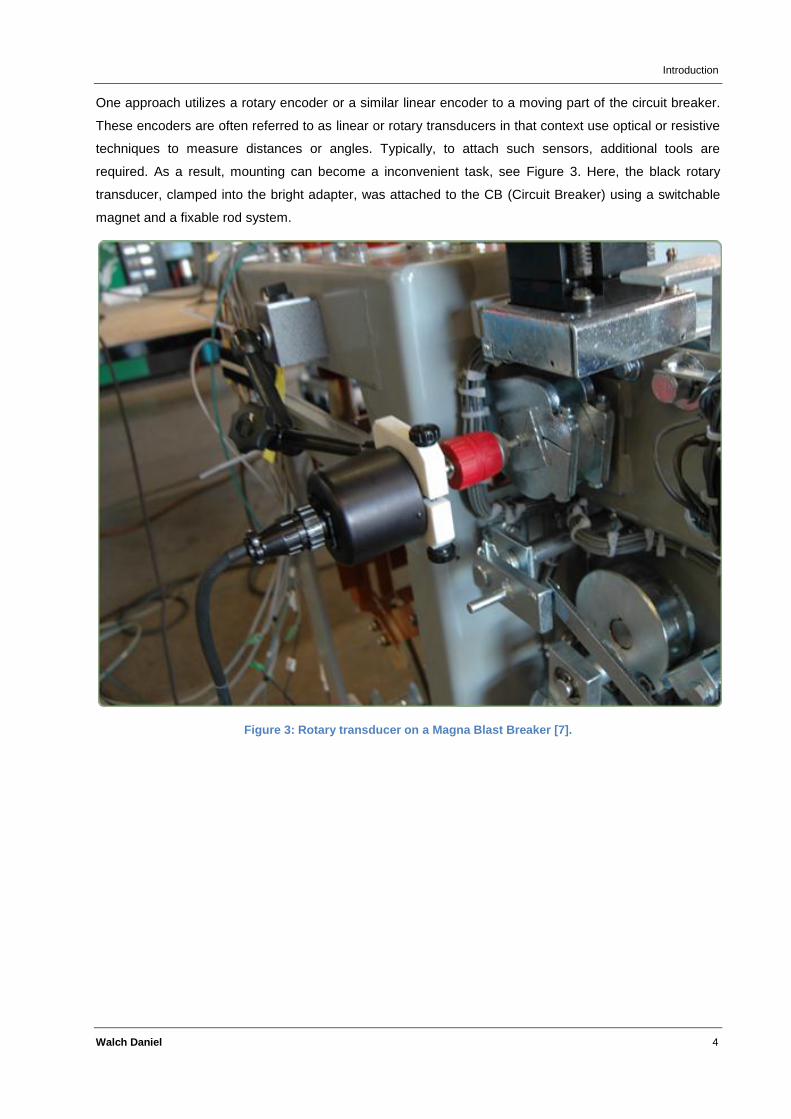
One approach utilizes a rotary encoder or a similar linear encoder to a moving part of the circuit breaker.
These encoders are often referred to as linear or rotary transducers in that context use optical or resistive
techniques to measure distances or angles. Typically, to attach such sensors, additional tools are
required. As a result, mounting can become a inconvenient task, see Figure 3. Here, the black rotary
transducer, clamped into the bright adapter, was attached to the CB (Circuit Breaker) using a switchable
magnet and a fixable rod system.
Figure 3: Rotary transducer on a Magna Blast Breaker [7].

Introduction
Walch Daniel 5
Using these transducers is a quite straight-forward approach to measure displacements of moving parts
and has advantages and disadvantages:
Advantages:
- Encoders are not too expensive (approximately 200 – 300 EUR)
- Easy processing of measurement data
Disadvantages:
- The accuracy may not be sufficient
- The sensor may be hard or even impossible to attach
- The method has a low cut-off frequency (approx. 2 kHz [8]) – knowledge about frequency
characteristics may get lost
- Measurement reproducibility can be a problem due to inconvenient mounting (hard to replicate)
- Measurement equipment using this approach is bulky.
The number of disadvantages suggests that it is possible to do better. This particular method is not very
convenient for the customer. The new solution shall be able to fulfill the task of the existing equipment and
at the same time ease mounting and handling. This is the motivation to write this thesis and propose
better methods to perform measurements of the displacement of the contacts in a high voltage circuit
breaker.

Problem description
Walch Daniel 6
2 Problem description
The aim is to measure the displacement of the contacts within a circuit breaker. The alternative solution
shall ease mounting and handling compared to traditional measurements with conventional transducers
while the quality of the measurement in terms of the key aspects stated below shall be maintained or even
improved. Since dismantling the device is usually not possible or desired, measurements have to be
carried out from the outside of the circuit breaker. Most often no knowledge about the inner parts of the
circuit breaker is available. Specifically, mechanical dimensions, relations, material characteristics etc. are
not described in any accessible document. Hence, no reliable statements about transmission ratios and
tolerances between pins and bushes can be made. As a result, it is not essential to determine the
absolute displacement, but rather to determine the relative displacement curve. If detailed information
about the circuit breaker’s mechanical assembly is given the test results can be re-scaled for comparison.
Still it’s interesting to what extent the alternative solution can determine the absolute displacement of the
moving part it’s attached to.
As mentioned in the previous chapter the conventional methods to measure the displacement of the
contacts in circuit breakers are not very convenient nor especially reliable or reproducible. The goal of this
thesis is to examine techniques that can fulfill certain demands, decide for one method for further
considerations and evaluate it.
The following key aspects are to be considered:
- Reproducibility – Do the results of consecutive measurements match?
- Accuracy – To what extent is it possible to determine the absolute displacement?
- Quality – How exactly does the shape of the final curve match the expected one?
- Attachment – What methods are suited best for attachment?
- Comparability – How does the new method compare to conventional ones?
2.1 Requirements
The solution presented within this paper should be capable of measuring the (relative) displacement curve
of the two contacts in a circuit breaker with focus on reproducibility, reliability, convenience to the user and
cost. Various measurement techniques shall be compared before selecting one of them. The selection
process shall consider the following aspects:
- Describing the switching process with a simplified model
- Presenting an approach to fulfill the task and pointing out advantages and disadvantages
- Considering parasitic effects and carrying out error estimates and reliability predictions

Problem description
Walch Daniel 7
- Designing an implementation and testing the whole concept in the field
- Evaluating the measurement results and comparing them with the expected ones
- Design a processing algorithm to analyze the raw data and present the results graphically
- Explaining any process effects that can be identified
- Finding a model (parameter set) for the displacement curve using optimization techniques
- Drawing conclusions, giving ideas for further improvement and highlighting future prospects
Measurement techniques
Walch Daniel 8
3 Measurement techniques
In this section, the measurement techniques that might satisfy the task within the given selection criteria
are investigated. A selection of the options available is given before reviewing and comparing them,
showing pros and cons of the proposed methods. Since there are a lot of ways to measure a distance or
rather the motion of a component, only some techniques are presented.
3.1 Conventional methods (encoders)
“Conventional” in this context means that the approaches presented in this chapter have already been
implemented – at least partially – in the given application or in similar fields of application.
3.1.1 Rotary and incremental encoders (transducers)
Rotary and incremental encoders are capable of determining a change in angle or location. Typically
these sensors have no absolute reference; hence absolute measurements are only possible when
referencing the sensor prior to the measurement.
There are very simple encoders available that are in principle potentiometers. These have an analog
output that is ratiometric with the distance or the angle. More sophisticated sensors have some “logic”
inside: The principle of such encoders is to determine the direction of the motion and to count “measuring
units” in the given direction. Each of these measuring units corresponds to a given length or angle. As a
result, it’s also possible to not only get analog quantities as an output but also as digital information.
Basically, the following methods are applied to construct a rotary or linear encoder:
Photoelectric encoders
Two principles are applied: The light beam of sources such as infrared/visible LEDs or laser diodes is
modulated by a sequence of light-impervious dashes followed by light-pervious areas on a disk. By using
at least two optical sensors the direction of the motion and the absolute or relative position can be
determined [9].
The second principle uses the effects of interferometry and bending when light travels through a lattice.
With these techniques an accuracy of down to a few micrometers and even less can be achieved [10].
Obviously, these encoder types could have also been considered in the section about optical methods.
Measurement techniques
Walch Daniel 9
Magnetic encoders
The principle of magnetic encoders is sensing magnetic material where magnetized areas alternate with
unmagnetized ones. Sensing is most often done by using Hall sensors or magneto resistive read heads.
The advantage of magnetic encoders is the (partial) insensitivity to pollution. Hence, such sensors are
often applied where encapsulating the measurement system is not possible or desired. Typically, the
smallest unit that can be measured is around a few micrometers whereas a spacing of some millimeters is
also possible [11].
Inductive encoders
These encoders use the principle of electromagnetic induction. Such encoders suffer from several
disadvantages such as temperature dependence of the magnetic material and sensitivity to the effects of
external magnetic fields, improvements though have been made [12].
Capacitive encoders
Capacitive encoders measure the capacitance between a scale and a reader [13], [14].
Encoders with sliding contacts (potentiometric sensors)
The operation principle is similar to a rotary switch. Again, the output of such sensors usually consists of
two 90 degree phase-shifted signals to determine direction and position. The advantage of encoders with
sliding contacts is the price, whereas accuracy and durability might suffer. To put it simply, in the analog
domain the device is nothing else than a potentiometer which changes its resistance dependent of the tap
position [15].
3.2 Optical methods
These methods use light and its characteristics to determine distances. Examples are given in section
3.1.1, where an incremental encoder using optical methods to determine displacement is described.
3.2.1 Triangulation
From the two ends of a baseline whose length is known the angles to the given point are measured. This
constellation forms a triangle where two angles and the length of one side are known. With this
information, all other values can be calculated. For the given application, typically a method known as
laser triangulation can be applied. A laser beam is focused on the object whose distance is to be
measured. At a known distance from the laser source a photosensitive element “tracks” the light dot.
When the distance to the object changes the light dot also appears at a different position. Using
trigonometric relations the distance from the laser source to the object can be found [16].
Measurement techniques
Walch Daniel 10
When talking about measuring the displacement of a moving part of a circuit breaker this method will
basically only work for objects that change their position (almost) linearly. If rotary motions occur the light
dot to be tracked will soon be out of (visual) range.
3.2.2 Travel time measurement
A light impulse is generated. After being reflected at an object the impulse is detected at the source. The
time it takes the light to travel from source to the object and back is proportional to the distance. Knowing
the elapsed time, the speed of light and the refractive index of the surrounding media (typically air) it’s
possible to determine the distance. Obviously, the accuracy of this method strongly depends on the
accuracy of the time measurement. One disadvantage of this method is that the time intervals to be
measured can become extremely small. As a result the accuracy of the time measurement must also be
extremely high what cannot always be achieved. This fact limits the smallest distance that can be
measured with that method. Understandably, the major application field is measuring distances in the
orders of kilometers. Still, several approaches have been made to increase the accuracy to the mm-level
[17]. Another drawback is the dependency on the surrounding media and its characteristics, in addition,
other objects beside the addressed one that reflect the signal also distort the measurement.
In the given application it’s necessary to measure distances in the order of a few centimeters, so this
method seems not to be very appropriate.
3.2.3 Phase measurement
The phase difference of a laser beam and its reflected version is dependent on the distance between the
sender and the reflecting object. Another option is to investigate the modulation of the reflected beam in
contrast to the original one. If the modulating frequency is the laser frequency the overall system is
referred to as laser interferometer. These interferometers are not capable of measuring the absolute
distance without additional information [18], page 3.
The advantage of this method is the high accuracy, typically in the nanometer region. Again, the
disadvantages are the low measuring range and that in the given application not only linear motions are
considered and it will not be possible to detect the reflected beam of a rotating object without great effort.
3.3 Image capturing methods
Another option is to film the object of interest and then determine the displacement using image
processing. Generally speaking, tracking a dot or something similar in images will be the task to fulfill what
is a well-known problem and would not cause significant difficulties. Other problems arise: Since the
Measurement techniques
Walch Daniel 11
switching operation of a circuit breaker is an extremely fast event, the camera to capture the pictures must
record many pictures per second and a high enough resolution to guarantee a satisfying accuracy. As a
result, the light to excite the sensor or film is only available for very short time intervals and thus the
sensitivity of the sensor or film has to be high, causing noise and other unwanted effects. This can be
avoided by brightening the region of interest with high-power lamps. Altogether the equipment cost will be
significantly higher compared to other methods.
3.4 Measuring using accelerometers
Inertial navigation utilizes accelerometers to determine absolute position. To be precise inertial navigation
systems (INS) require six quantities to determine the actual position in space: three acceleration and three
angular velocity signals [19]. If things can be simplified by making certain constraints, the rotation rate
sensors can be ignored and only accelerometers can be used. Dependent on the number of
accelerometers, displacements in up to three dimensions (in space) can be measured. The acceleration
signal is integrated once to get the velocity and twice to get the displacement. The advantage of this
method is the pretty straight-forward approach; the drawback is that by integrating the measurement
signal twice also all errors are integrated. This leads to strong deviations in the final displacement result.
In practice, when talking for example about navigation, such systems have to be updated and referenced
regularly with information from other sources such as GPS. Fully autonomous systems that use only
accelerometers for determining the position are not very reliable.
3.5 Decision matrix
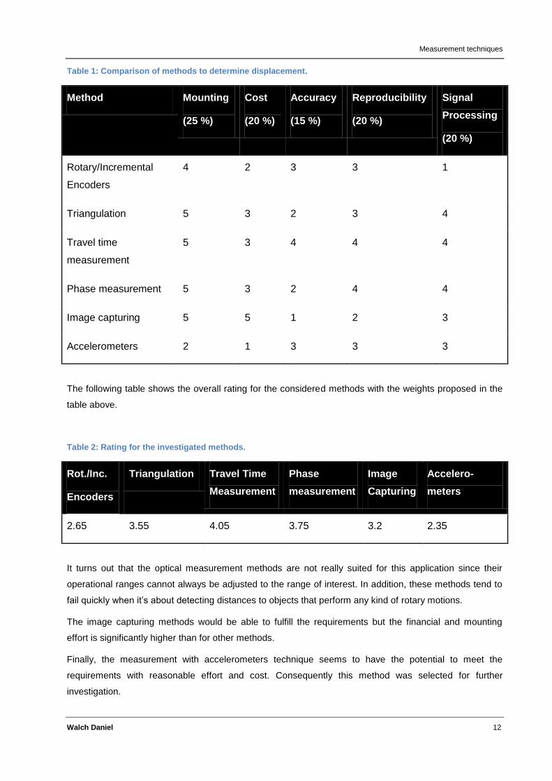
In order to better understand the characteristics as well as the advantages and disadvantages of the
applicable methods shown above, a comparative matrix has been generated. The aspects are valued
using numbers from 1 to 5, where 1 represents the best/cheapest/most convenient solution whereas a 5
stands for worst/most expensive/inconvenient method. The numbers are estimates and base on personal
experience and information given by manufacturers
One could argue that some of the methods do not meet the “convenience” requirement that might be
considered as mandatory. This is principally true; but since not many methods with higher mounting
convenience compared to the technique using displacement transducers are available, they have been
considered anyway and graded with a low rating with respect to the mounting criterion.
Measurement techniques
Walch Daniel 12
Table 1: Comparison of methods to determine displacement.
Method Mounting
(25 %)
Cost
(20 %)
Accuracy
(15 %)
Reproducibility
(20 %)
Signal
Processing
(20 %)
Rotary/Incremental
Encoders
4 2 3 3 1
Triangulation 5 3 2 3 4
Travel time
measurement
5 3 4 4 4
Phase measurement 5 3 2 4 4
Image capturing 5 5 1 2 3
Accelerometers 2 1 3 3 3
The following table shows the overall rating for the considered methods with the weights proposed in the
table above.
Table 2: Rating for the investigated methods.
Rot./Inc.
Encoders
Triangulation Travel Time
Measurement
Phase
measurement
Image
Capturing
Accelero-
meters
2.65 3.55 4.05 3.75 3.2 2.35
It turns out that the optical measurement methods are not really suited for this application since their
operational ranges cannot always be adjusted to the range of interest. In addition, these methods tend to
fail quickly when it’s about detecting distances to objects that perform any kind of rotary motions.
The image capturing methods would be able to fulfill the requirements but the financial and mounting
effort is significantly higher than for other methods.
Finally, the measurement with accelerometers technique seems to have the potential to meet the
requirements with reasonable effort and cost. Consequently this method was selected for further
investigation.

Related work
Walch Daniel 13
4 Related work
In this section, some of the related work that has dealt with circuit breaker testing or determining
displacement from acceleration data is presented. There are a vast number of publications available on
these topics, for example in the IEEE library. The work presented below is just an excerpt.
4.1 Circuit breakers and circuit breaker testing
In the last two decades, two measurement techniques have turned out to be particularly important: Firstly,
measuring timing during a switching operation (on/off time) by analyzing voltage/current behavior also
referred to as “dynamic contact resistance measurement (DRM)” where the resistance between the
connections of a CB during a switching operation is determined. Secondly, a motion analysis carried out
by attaching a sensor to a moving part of the CB. The result of this measurement is a travel curve that
reproduces to the travel of the switching contacts dependent on the mechanical relations between the
place of attachment and the contacts.
Theory and design of circuit breakers is presented in the book by C. H. Flurscheim [20]. A short
introduction to circuit breaker testing is given in [5].
Circuit breaker testing has been an issue from the early days of electrification on to the present. For
example, an early work discussing the progress on researching on circuit breaking was published in 1929
[21].
An introduction to air-blast circuit breakers from the year 1952 is given in [22], whereas a vacuum circuit
breaker is investigated in the work by Y. Niwa et al. [2]. The topic “technical and physical feasibility versus
economic efficiency of high voltage vacuum interrupters” is discussed in [23].
R. P. P. Smeets and W. A. van der Linden published an article dealing with the testing of SF6 generator
circuit breakers [24].
One reason for carrying out DRM is to determine the condition of the contacts. Basic requirements and
design suggestions are given in the paper by L. C. Campbell [25]. An excursion on erosion of Cu/W
contacts is presented in [26], whereas the physical processes that occur when opening the contacts is
given in [27].
A common practice is trying to analyze the state of a circuit breaker after a short-circuit event before
putting it back into operation. In [28], the authors suggest two methods to ensure the circuit breaker is in a
good condition: modal identification and off-line diagnosis methods such as vibration analysis.

Related work
Walch Daniel 14
A monitoring system based on the principle of electromagnetic induction is described in [29], supported by
microcontrollers. Another approach, given in [30], also makes use of microprocessors. It’s stated that a
number of parameters such as velocity, stroke, penetration of the contact, etc. can be determined. By
comparing these parameters to those of previous measurements, a trend can possibly be identified and
appropriate actions can be taken.
An interesting approach to investigating contact travel, gas pressure and particle concentration in SF6
puffer circuit breakers is given in [31]. The authors present a method that uses optical fibers.
Several sensing techniques to periodically or continuously monitoring parameters within a circuit breaker
are presented in various documents. In [32], for example, a new sensing technique is proposed,
employing remote temperature measurement and emission spectrum detection.
In [33] strategies of attacking the problem of carrying out an efficient DRM are presented. The authors
present an approach that deals with the problems that occur when metallic fluorides are present. These
are produced during the arc quenching process and mask the actual breaker contact resistance.
Two of the authors have, among others, published another paper that deals with the same topic. A new
measurement method of the dynamic contact resistance of HV circuit breakers is presented. They state
that with this novel method the DRM curve is easy to interpret and allows reproducible resistance curves
[34]. Similar material can be found in [35], the presentation slides of the IEEE/PES Switchgear Committee
Meeting in Montreal, 2005.
A detailed model of a high voltage CB has been introduced within the dissertation of B. Rusek. In the
thesis the model is introduced and helps to identify and to study effects of certain processes and failures
that cannot be investigated in reality because of safety and cost [36]. There is also a book available with
the same title.
An excursion on the relationship between displacement characteristics of a given vacuum-type CB and
spring type operating mechanism, as applied in many CBs, is done in [37].
A test system for determining timings during a switching operation is proposed in [38].
An overview on testing of vacuum CBs with focus on specific issues and developments is presented in a
paper published in 1998 [39]. In the same year, the lead author also wrote about testing of SF6 generator
CBs [24].
An application where accelerometers are actually used in connection with circuit breaker testing is
vibration analysis [40]. The approach to determine vibrations by evaluating the acceleration signal is
known from other applications.

Related work
Walch Daniel 15
4.2 Acceleration, velocity, displacement, and positioning
Since the acceleration signal is represented by a number of measured values within a test series and not
as an analytic function, integration has to be performed numerically. Several methods have been invented
and thoroughly evaluated so there is a large amount of material available. A review of some of the work
carried out on this topic is presented below.
As mentioned earlier, evaluating acceleration signal is often a task used in positioning and tracking.
Navigation systems, such as used in airplanes, use gyro meters and accelerometers. For determining the
displacement of the contacts within a CB it’s not necessary to apply gyro meters since the absolute travel
distance is low and the motion curve itself is not very complicated. In addition, the system can be
calibrated regularly - after each switching operation. Still, it’s interesting how the well-known problems of
accuracy, drifts and others have been attacked in previous works.
An inertial measuring unit is investigated in [41], the focus is put on low-cost. It turns out that low-cost
systems are capable of meeting the same functional requirements as high-accuracy systems, except of
long-term position.
A dissertation about a variable-step double-integration multi-step integrator was written by Matthew M.
Berry [42]. The method presented in the thesis is the variable-step Störmer-Cowell method and uses error
control to regulate the step size.
In [43], the authors present a system for mobile robot positioning using accelerometers. The problem of
bias drift problems is attacked by Kalman filtering to improve the results. It is worth considering
implementing this technique in this thesis.
The problem of long-term drifts is addressed in [44]. What’s interesting about this publication is that
analog integrators have been used. Two approaches have been made with the conclusion that a critically
damped double integrator coupled with an accelerometer is well-suited for frequency domain system
identification.
In [45], K. V. Ramachandra deals with obtaining position, velocity and acceleration from noisy radar
measurements. Kalman filtering is also applied in this work.
Another positioning system is proposed in [46]. To determine the position, acceleration signal and moving
direction are considered.
The topic “Remote Sensing of Position and Acceleration is addressed in [47]. The author uses a PsoC
(Programmable System on Chip) with RTC (real time clock) and the necessary links to transmit data. The
accelerometer in use was manufactured by Analog Devices.
MEMS technology has been evolving in the last years. An approach to design a MEMS based capacitive
accelerometer is presented in [48].
Related work
Walch Daniel 16
A solid-state accelerometer for positioning of a vehicle is evaluated by three authors from Iran [49]. Again,
they use Kalman filtering in combination with smoothing algorithms to compensate for long-term errors.
Similar topics are discussed in [50]. The authors focus on the evaluation of acceleration sensor errors for
better position estimation using acceleration bias drift error model. As in [49], they also apply Kalman
filtering together with smoothing.
The CMOS-MEMS accelerometer introduced in [51] is capable of measuring three axes and focuses on
the design of the device using CMOS technology. It includes accelerator sensing method of the z-axis.
4.3 Comment
What will be seen later is that bias and random drifts of the accelerometers are some of the main
challenges to be mastered in designing the measurement system. This is because the result of long-term
double integration of measured acceleration usually deteriorates as the integration period becomes larger.
From the literature given above two approaches turn out to appear regularly when dealing with this
problem in positioning applications: Kalman filtering (with smoothing) and frequent (re-)calibration.
The latter “resets” the position information to a known state and sets the error in the position information
virtually to zero. In positioning and navigation, the information to calibrate the position is most often
gathered from the GPS (Global Positioning System). In CB testing, calibration with GPS is not an option
because the accuracy is not high enough. On the other hand, the measurement time is in the order of a
few seconds and calibration can be done prior to each measurement. Hence, the task will be to eliminate
any short-time drifts that might affect the measurement.
Kalman filtering in that context is usually implemented to remove noise and bias from the measurement
samples [49]. In the given application it would also be an option to implement Kalman filtering. Though, a
different technique has been applied as will be seen later. As the evaluation can be done off-line, it is not
necessary to use a causal filter. Based on this, the entire signal can be considered for processing. This
advantage is exploited in the method applied within this thesis.

Accelerometers
Walch Daniel 17
5 Accelerometers
In this chapter the characteristics of various accelerometers and their functional principles are discussed.
Quantitative requirements from the application are estimated. After a short market overview the pros and
cons of different accelerometers are pointed out.
5.1 Types and applicability
Various types and models of accelerometers are available from a number of manufacturers. In recent
years capacitive, piezoresistive/-electric and MEMS devices have captured the market.
5.1.1 Magnetic Induction
The principle is similar to a plunger coil microphone. A magnet connected to a spring is moving within the
inner diameter of a coil and inducting a voltage [52], [53].
5.1.2 Capacitive
The seismic mass is placed between the plates of a capacitor (differential capacitor) and acts as an
electrode. When it experiences a displacement due to acceleration, the distances of the plates of the
capacitors change. This deviation in capacitance can be observed and is used to determine the
acceleration [53]. This principle is also applied in MEMS sensors, see section 5.1.3.

Accelerometers
Walch Daniel 18
Figure 4: Principle of a capacitive accelerometer
Capacitive sensors are capable of measuring both static and dynamic accelerations.
5.1.3 MEMS
MEMS is short for micro-electro-mechanical system. MEMSs are usually made of silicon and often a
“simple” spring-mass system is manufactured internally. Both the spring (consisting of small (~ µm) silicon
bars) and the mass are made in silicon. If there is a displacement between the springy part and the fixed
part, a change in electrical capacitance can be measured [54]. The FSR is usually typically very low which
requires that the evaluation electronics be on chip.
Dependent on the principle applied (piezoelectric effect, capacitance, etc.) a MEMS accelerometer can be
capable of measuring static accelerations.
The following two types are considered as members of the MEMS group although they could also be
manufactured in larger scale with the same technique.
5.1.3.1 Piezoelectric
A seismic mass is fixed to a piezoceramic material. If the system experiences acceleration, the seismic
mass compresses/stretches the piezoceramic material, which causes electric charge to be detectable at
the electrodes [53].

Accelerometers
Walch Daniel 19
Figure 5: Principle of a piezoelectric accelerometer
Piezoelectric devices can’t detect static accelerations since in practice a discharge process will occur by
leakage current through the measurement device or the attached charging amplifier.
5.1.3.2 Piezoresistive
When the seismic mass is experiencing acceleration it deforms its suspension. The piezoresistors
mounted on this suspension change their resistance value accordingly. This change in resistance is
usually determined by using full bridge measurement circuitry. This technique is also referred to as
resistive strain gauge and is primarily used in low frequency and small acceleration amplitude applications
[53].
Due to the architecture, piezoresistive sensors are capable of measuring both static and dynamic
accelerations.
5.1.4 Temperature
Such sensors consist of a chamber filled with gas, a heating element in the middle and temperature
sensors applied at the “edges” of the chamber. Hot gas rises whereas cold gas sinks. When tilting the
sensor, the hot gas moves towards the corresponding area of the chamber. The temperature sensors
measure a hotter/colder temperature accordingly. In general, the characteristics of these sensors are
inferior compared to the ones described above [55].
Temperature sensors are capable of measuring both static and dynamic accelerations.

Accelerometers
Walch Daniel 20
5.1.5 Rarely used techniques
- sensitive axis with slidable mass (very first types of accelerometers) [52]
- bendable quartz-rod (“Q-flex”) [52]
- magnetically stabilized mass systems [52]
- Sensors applying the Ferraris principle [56]
This list makes no claims of being complete but represents an excerpt of the most commonly used
techniques. In most technical applications nowadays, MEMS sensors are used.
Accelerometers
Walch Daniel 21
5.2 Sensor requirements
The requirements on the sensor are determined by the application. Since measuring the displacement of
the contacts of circuit breakers with accelerometers has never been applied in this context, it is only
possible to estimate the constraints set up by the application.
5.2.1 Measuring range
Since the approximate switching time and distance to be covered by the contacts are known the
acceleration that the sensor must be capable of measuring can be estimated. Circuit breaker switching
operations are very fast transient events where high accelerations occur. Obviously, the acceleration is
also dependent on the mounting position. If the distance the sensor travels has about the same dimension
as the stroke of the contacts, the maximum possible acceleration can be limited to around 500 g where g
represents the g-force of approximately 9.81 ms-2
. Obviously, the acceleration is strongly dependent on
the attachment location.
5.2.2 Sensitivity
The term “sensitivity” is used in two contexts: Firstly, it can define the ratio between input and output of
the sensor. Thus, the sensitivity is typically given in C/g or V/g, depending whether the charge amplifier
circuitry is on chip or not. Secondly, sensitivity can be referred to as discrimination threshold. To put it
simply, that’s the least excitation at the input that can be observed at the output of the sensor. This
quantity is most often directly related to the noise of the sensor and is therefore addressed in chapter
5.2.6 whereas in this chapter the first definition of this term is considered.
In general, a high SNR is desired. When assuming the noise of the sensor to be given, the sensitivity is
desired to be high, improving the SNR. Unfortunately, measuring range and sensitivity are inversely
proportional. Often, the sensitivity is linearly dependent on the supply voltage. Hence, increasing the
supply voltage to the upper limit of the operational range will help to increase the sensitivity. The typical
sensitivity of a sensor with +/- 500 g measurement range is 10 mV/g for sensors with voltage output.
5.2.3 Offset
The offset generated by the sensor itself is not of big concern since it can be eliminated from the
measurement signal if it’s approximately constant during the measurement. The offset error is also
depicted in Figure 6.
Accelerometers
Walch Daniel 22
5.2.4 Offset drift
The measurement time is in the range of a few seconds. All drifts that are constant during this time
interval can easily be eliminated. As a result, offset drifts of any kind (temperature, aging, etc.) must be
slow compared to the measurement time.
As a rule of thumb one can state that offset drifts of a frequency in the dimension of up to a few Hertz can
be eliminated by signal processing since it’s obvious that such acceleration signals are not generated by
the switching process itself. In principle, a high-pass filter with a low corner frequency (a few Hertz) can be
applied to eliminate such drifts from the measurement signal.
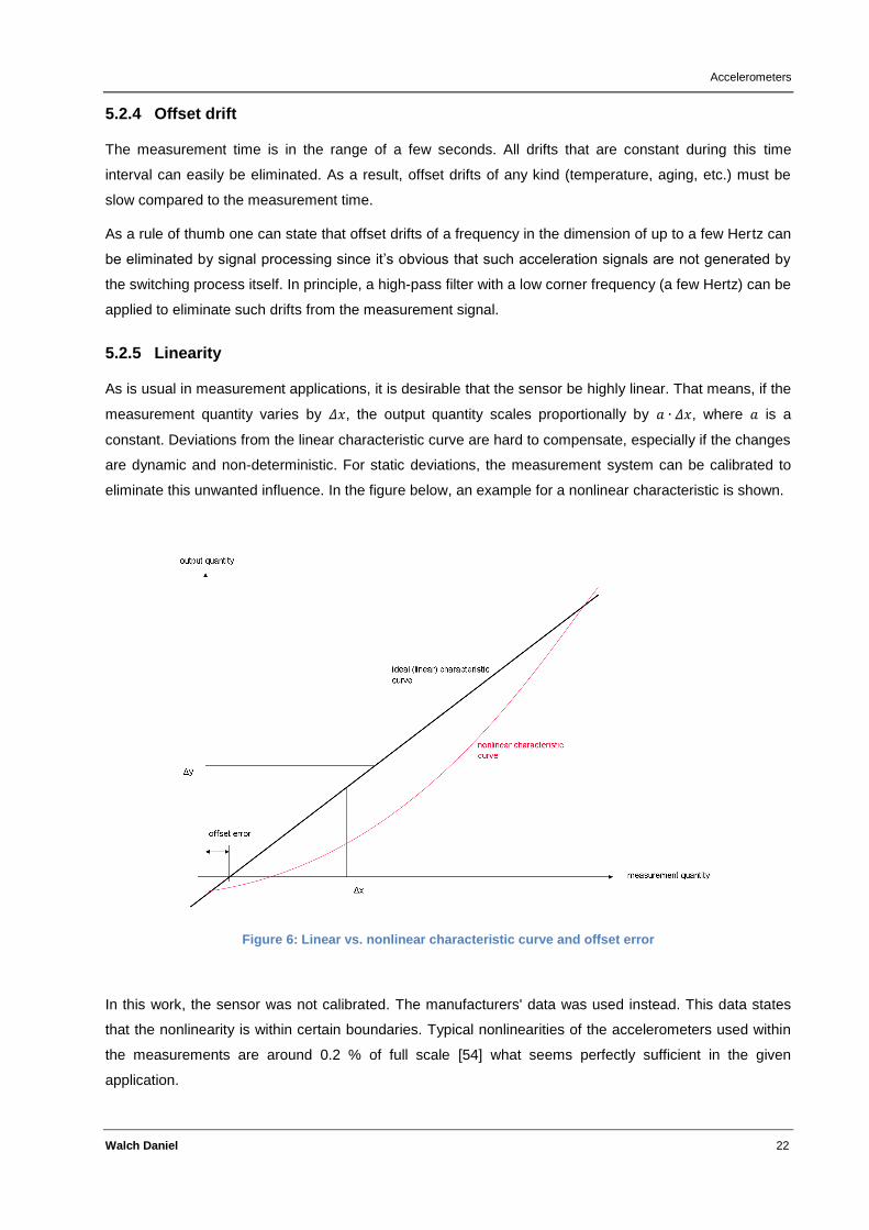
5.2.5 Linearity
As is usual in measurement applications, it is desirable that the sensor be highly linear. That means, if the
measurement quantity varies by , the output quantity scales proportionally by , where is a
constant. Deviations from the linear characteristic curve are hard to compensate, especially if the changes
are dynamic and non-deterministic. For static deviations, the measurement system can be calibrated to
eliminate this unwanted influence. In the figure below, an example for a nonlinear characteristic is shown.
Figure 6: Linear vs. nonlinear characteristic curve and offset error
In this work, the sensor was not calibrated. The manufacturers' data was used instead. This data states
that the nonlinearity is within certain boundaries. Typical nonlinearities of the accelerometers used within
the measurements are around 0.2 % of full scale [54] what seems perfectly sufficient in the given
application.
Accelerometers
Walch Daniel 23
5.2.6 Noise
Since the acceleration signal itself is integrated twice to yield displacement, the noise density will not be of
big concern. The reasoning that noise will typically not affect the displacement too much is given in
chapter 6.2.5. In this chapter it will be shown that the noise or the noise density of a sensor will not be a
knock-out criterion for any of the available sensors. Since the manufacturer’s information on residual
noise or residual noise densities are not consistent it’s hard to compare one sensor to another. Typically,
noise densities are given for certain frequency (in √ ) or the RMS value for the residual noise is
specified (in g equivalents) for the sensor’s bandwidth. Some manufacturers prefer to specify noise in
terms of output voltage.
5.2.7 Frequency response
Estimations suggest that the upper cutoff frequency should be above 5 kHz, but it’s not necessary for the
cutoff frequency to exceed 20 kHz since the maximum sampling frequency will be chosen as 40 kHz. If
also static accelerations such as gravity must be detected, the lower cutoff frequency must be 0 Hz (DC).
Sensors that are not capable of measuring static accelerations can have a lower cutoff frequency of a few
Hertz. Choosing the cutoff frequency such, accelerations that are not caused by the switching operation
itself can be eliminated since the sensor will not detect them.
5.2.8 Cross-Axis sensitivity
The sensitivity to accelerations that are not in the direction of the “sensitive axis” should be as low as
possible. Typically, the cross-axis sensitivity of a sensor is around a few percent [54]. Since the mounting
uncertainty will usually be much greater, the cross-axis sensitivity of the sensor will be overlaid and
therefore the effect will hardly be visible in the results.
5.2.9 Temperature Sensitivity
As long as the temperature dependency is linear, sensitivity to temperature changes is not a problem in
the given application. It can be assumed that the temperature doesn’t change much during one
measurement cycle and therefore temperature sensitivity does not play a big role. However, temperature
may change to a significant extent from one measurement to another, especially when they are separated
by a great amount of time. This can easily happen when considering measurements carried out when
performing maintenance operations. If this happens, at least the shape of the curve should be similar
since it can be assumed that the temperature coefficient is affecting the sensitivity of the sensor linearly
with temperature. A typical value for the temperature coefficient of sensitivity is 0.05 %/K [57].

Accelerometers
Walch Daniel 24
5.2.10 Load
The sensor’s output should be capable of being connected to the input of an ADC with some capacitance.
Typically, this is in the range of a few nF. If this capacitive load is too high, an impedance converter
should be attached to solve the problem.
5.2.11 Output type
Available accelerometers have either a voltage or charge output. Accelerometers with a voltage output
have the charge amplifier and converter integrated into the sensor. For MEMS types this is on the same
chip.
Since it’s not desirable to use an external charge amplifier in the application, only sensors with voltage
output are considered.
5.2.12 Size and weight
The device under test should not be influenced by the accelerometer. In this particular application, the
contacts sizes and weights are well above that of the accelerometer. Still, it’s advantageous for the
sensors to be small and light weight because the requirements on the mechanical bond to the device
under test can be relaxed. A weight below 20 grams and a size that not exceeds exceed 3 cm x 3 cm x 3
cm will lead to reasonably convenient mounting.
5.2.13 Number of axes
Accelerometers can have one, two, or three sensitive axes. Usually the multiaxial sensors consist of
uniaxial sensors that have been mechanically arranged to form a two- or three-axes overall sensor. For
the given application motion is restricted to a plane in space and hence only two-axial sensors are
necessary. When the absolute displacement curve of the sensor itself is not of interest even uniaxial
sensors would be sufficient since it’s known that the contacts of the circuit breaker will only move linearly,
in one dimension. As a result, only uniaxial accelerometers were considered.
Later it turned out that the influence of gravity can be seen in the final displacement curve. With some
effort it’s at least partly possible to compensate for that effect even when using uniaxial sensors.
Obviously, when tracking two axes, eliminating the influence of the g-force would be easier and also
possible for more general curves. From a financial point of view it would be advantageous to stick to
sensors with only one axis.
Accelerometers
Walch Daniel 25
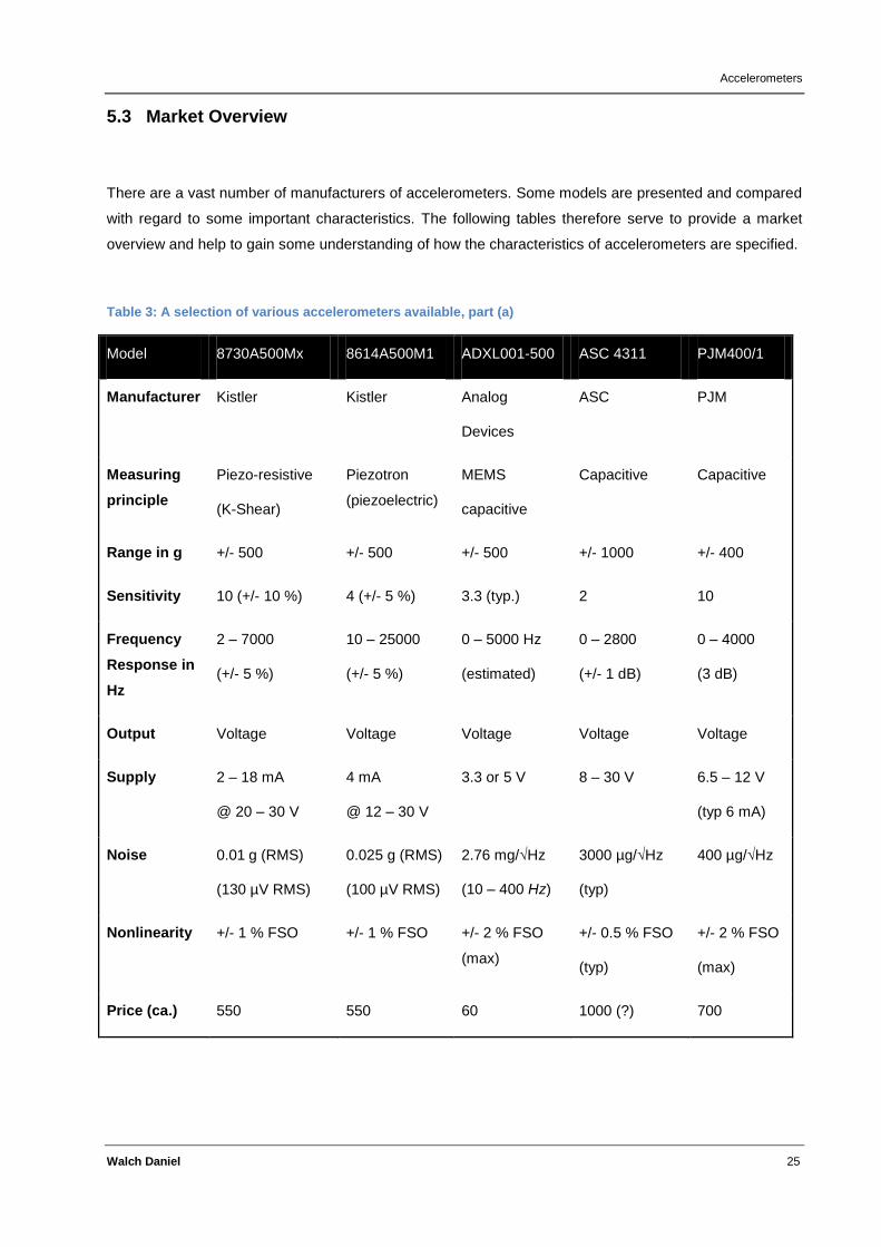
5.3 Market Overview
There are a vast number of manufacturers of accelerometers. Some models are presented and compared
with regard to some important characteristics. The following tables therefore serve to provide a market
overview and help to gain some understanding of how the characteristics of accelerometers are specified.
Table 3: A selection of various accelerometers available, part (a)
Model 8730A500Mx 8614A500M1 ADXL001-500 ASC 4311 PJM400/1
Manufacturer Kistler Kistler Analog
Devices
ASC PJM
Measuring
principle
Piezo-resistive
(K-Shear)
Piezotron
(piezoelectric)
MEMS
capacitive
Capacitive Capacitive
Range in g +/- 500 +/- 500 +/- 500 +/- 1000 +/- 400
Sensitivity 10 (+/- 10 %) 4 (+/- 5 %) 3.3 (typ.) 2 10
Frequency
Response in
Hz
2 – 7000
(+/- 5 %)
10 – 25000
(+/- 5 %)
0 – 5000 Hz
(estimated)
0 – 2800
(+/- 1 dB)
0 – 4000
(3 dB)
Output Voltage Voltage Voltage Voltage Voltage
Supply 2 – 18 mA
@ 20 – 30 V
4 mA
@ 12 – 30 V
3.3 or 5 V 8 – 30 V 6.5 – 12 V
(typ 6 mA)
Noise 0.01 g (RMS)
(130 µV RMS)
0.025 g (RMS)
(100 µV RMS)
2.76 mg/√Hz
(10 – 400 Hz)
3000 µg/√Hz
(typ)
400 µg/√Hz
Nonlinearity +/- 1 % FSO +/- 1 % FSO +/- 2 % FSO
(max)
+/- 0.5 % FSO
(typ)
+/- 2 % FSO
(max)
Price (ca.) 550 550 60 1000 (?) 700
Accelerometers
Walch Daniel 26
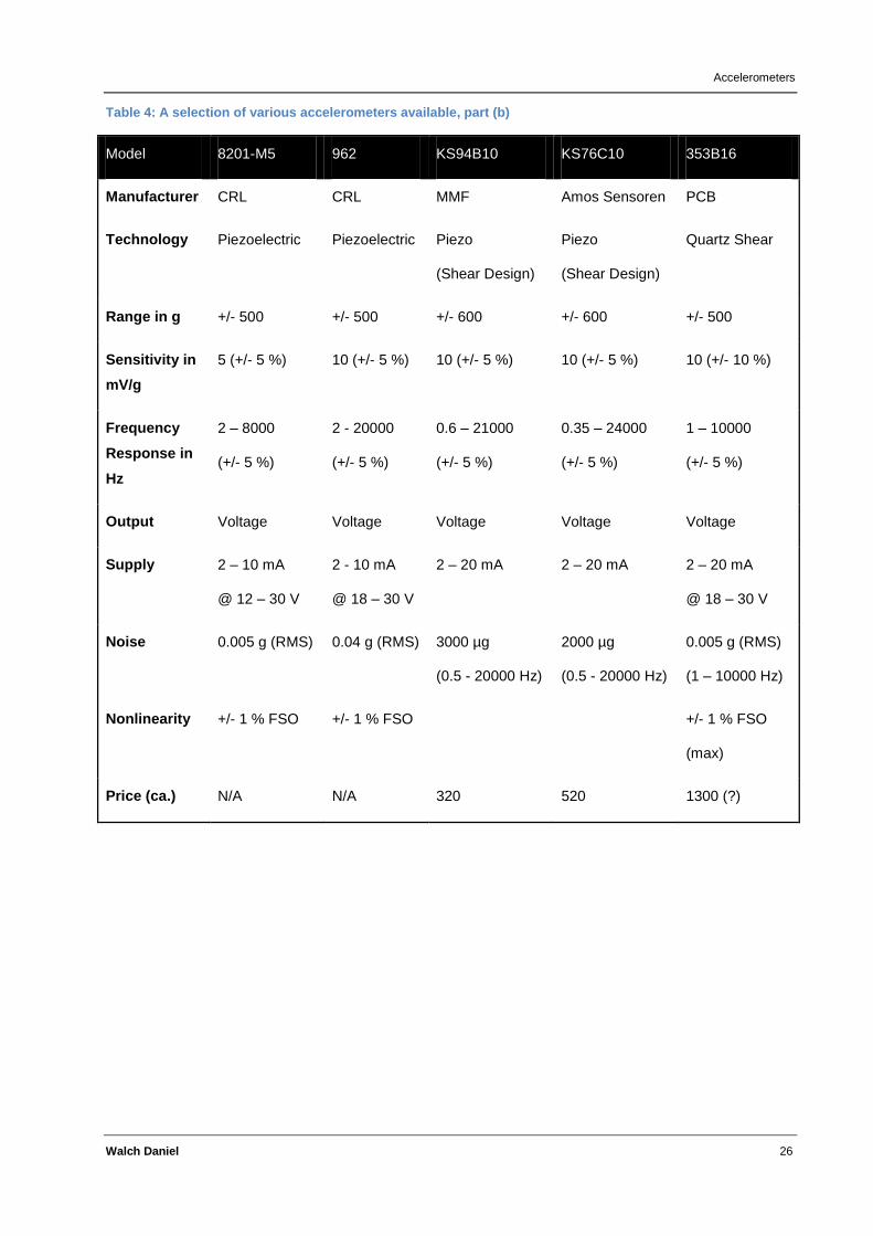
Table 4: A selection of various accelerometers available, part (b)
Model 8201-M5 962 KS94B10 KS76C10 353B16
Manufacturer CRL CRL MMF Amos Sensoren PCB
Technology Piezoelectric Piezoelectric Piezo
(Shear Design)
Piezo
(Shear Design)
Quartz Shear
Range in g +/- 500 +/- 500 +/- 600 +/- 600 +/- 500
Sensitivity in
mV/g
5 (+/- 5 %) 10 (+/- 5 %) 10 (+/- 5 %) 10 (+/- 5 %) 10 (+/- 10 %)
Frequency
Response in
Hz
2 – 8000
(+/- 5 %)
2 - 20000
(+/- 5 %)
0.6 – 21000
(+/- 5 %)
0.35 – 24000
(+/- 5 %)
1 – 10000
(+/- 5 %)
Output Voltage Voltage Voltage Voltage Voltage
Supply 2 – 10 mA
@ 12 – 30 V
2 - 10 mA
@ 18 – 30 V
2 – 20 mA 2 – 20 mA 2 – 20 mA
@ 18 – 30 V
Noise 0.005 g (RMS) 0.04 g (RMS) 3000 µg
(0.5 - 20000 Hz)
2000 µg
(0.5 - 20000 Hz)
0.005 g (RMS)
(1 – 10000 Hz)
Nonlinearity +/- 1 % FSO +/- 1 % FSO +/- 1 % FSO
(max)
Price (ca.) N/A N/A 320 520 1300 (?)
Accelerometers
Walch Daniel 27
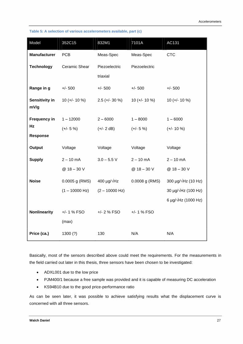
Table 5: A selection of various accelerometers available, part (c)
Model 352C15 832M1 7101A AC131
Manufacturer PCB Meas-Spec Meas-Spec CTC
Technology Ceramic Shear Piezoelectric
triaxial
Piezoelectric
Range in g +/- 500 +/- 500 +/- 500 +/- 500
Sensitivity in
mV/g
10 (+/- 10 %) 2.5 (+/- 30 %) 10 (+/- 10 %) 10 (+/- 10 %)
Frequency in
Hz
Response
1 – 12000
(+/- 5 %)
2 – 6000
(+/- 2 dB)
1 – 8000
(+/- 5 %)
1 – 6000
(+/- 10 %)
Output Voltage Voltage Voltage Voltage
Supply 2 – 10 mA
@ 18 – 30 V
3.0 – 5.5 V 2 – 10 mA
@ 18 – 30 V
2 – 10 mA
@ 18 – 30 V
Noise 0.0005 g (RMS)
(1 – 10000 Hz)
400 µg/√Hz
(2 – 10000 Hz)
0.0008 g (RMS) 300 µg/√Hz (10 Hz)
30 µg/√Hz (100 Hz)
6 µg/√Hz (1000 Hz)
Nonlinearity +/- 1 % FSO
(max)
+/- 2 % FSO +/- 1 % FSO
Price (ca.) 1300 (?) 130 N/A N/A
Basically, most of the sensors described above could meet the requirements. For the measurements in
the field carried out later in this thesis, three sensors have been chosen to be investigated:
ADXL001 due to the low price
PJM400/1 because a free sample was provided and it is capable of measuring DC acceleration
KS94B10 due to the good price-performance ratio
As can be seen later, it was possible to achieve satisfying results what the displacement curve is
concerned with all three sensors.
Approach
Walch Daniel 28
6 Approach
In this section the approach to actually invent an innovative measuring system for circuit breakers is
presented. The focus is put on the accelerometer method. First, a simplified model to describe the
processes occurring during the switching process of a circuit breaker is introduced. Sources of parasitic
effects are identified and described and some error estimates are carried out in the next step. Eventually,
the concept is tested in the field and an analysis of the measurement data is done. The problems,
uncertainties and challenges when going from an acceleration signal to the position or displacement
information are pointed out and discussed. After that, in subsequent chapters, the method of choice is
assessed and compared to the conventional method. Finally, an exhaustive review of the overall system
is carried out and the compliance to the prerequisites initially set up are checked.
6.1 Simple model
A simplified model to describe the events occurring when a switching action takes place in a circuit
breaker consists of springs, masses and dampers only. It shall serve to make fundamental statements
about the characteristics of the switching operation and the resulting displacement curve. As will be seen,
such a simple model is not suitable to describe all the effects visible in the displacement curve but it will
help to develop some basic understanding of the functioning principle of a CB and lead to reasonable
assumptions what the driving spring is concerned.
A switching operation is divided into two parts: When the contacts start their movement and the contacts
gain velocity and when they start colliding with the damping contact and settle in the final position. Since
many circuit breakers are operated using a strong mechanical spring that can be pre-stressed with an
electric motor, the driving mechanism is modeled by a spring. All the mechanical components between
the spring and the place where the acceleration data is tapped can be modeled by another mass and an
attached spring that simulates the lag between the moving end of the spring and the sensor’s attachment
place and the oscillations that can be caused due to the strong mechanical excitation. Combining this
second spring with a damper gives the opportunity to also model the decaying characteristic of this
parasitic oscillation. The collision with the rebound contact can again be modeled by a parallel
arrangement of an extremely hard spring and a strong damper.
Since first estimates suggest that the spring isn’t relaxed significantly during one switching process, the
spring force generated by k1 can be considered constant. This fact will be regarded when a simple
estimate about the shape of the displacement curve is done.
Approach
Walch Daniel 29
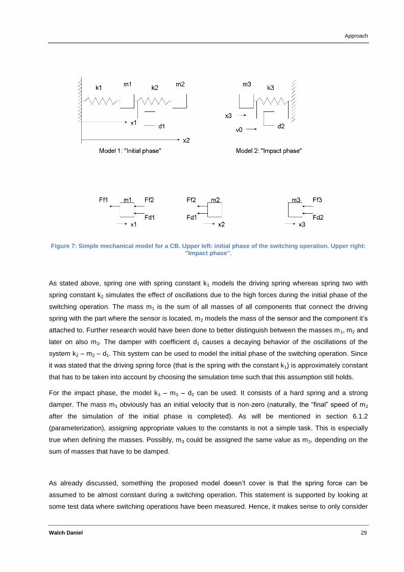
Figure 7: Simple mechanical model for a CB. Upper left: initial phase of the switching operation. Upper right: "Impact phase".
As stated above, spring one with spring constant k1 models the driving spring whereas spring two with
spring constant k2 simulates the effect of oscillations due to the high forces during the initial phase of the
switching operation. The mass m1 is the sum of all masses of all components that connect the driving
spring with the part where the sensor is located, m2 models the mass of the sensor and the component it’s
attached to. Further research would have been done to better distinguish between the masses m1, m2 and
later on also m3. The damper with coefficient d1 causes a decaying behavior of the oscillations of the
system k2 – m2 – d1. This system can be used to model the initial phase of the switching operation. Since
it was stated that the driving spring force (that is the spring with the constant k1) is approximately constant
that has to be taken into account by choosing the simulation time such that this assumption still holds.
For the impact phase, the model k3 – m3 – d2 can be used. It consists of a hard spring and a strong
damper. The mass m3 obviously has an initial velocity that is non-zero (naturally, the “final” speed of m2
after the simulation of the initial phase is completed). As will be mentioned in section 6.1.2
(parameterization), assigning appropriate values to the constants is not a simple task. This is especially
true when defining the masses. Possibly, m3 could be assigned the same value as m2, depending on the
sum of masses that have to be damped.
As already discussed, something the proposed model doesn’t cover is that the spring force can be
assumed to be almost constant during a switching operation. This statement is supported by looking at
some test data where switching operations have been measured. Hence, it makes sense to only consider
Approach
Walch Daniel 30
the very first part of the simulation results around t = 0, where the spring force (and therefore the
acceleration) can be linearized. To simulate a full switching operation, one has to record the parameters
(i. e., velocity) at the end of the initial phase and then feed these into the second model, namely model 2
that then simulates the impact phase. Finally, both simulation curves have to be linked.
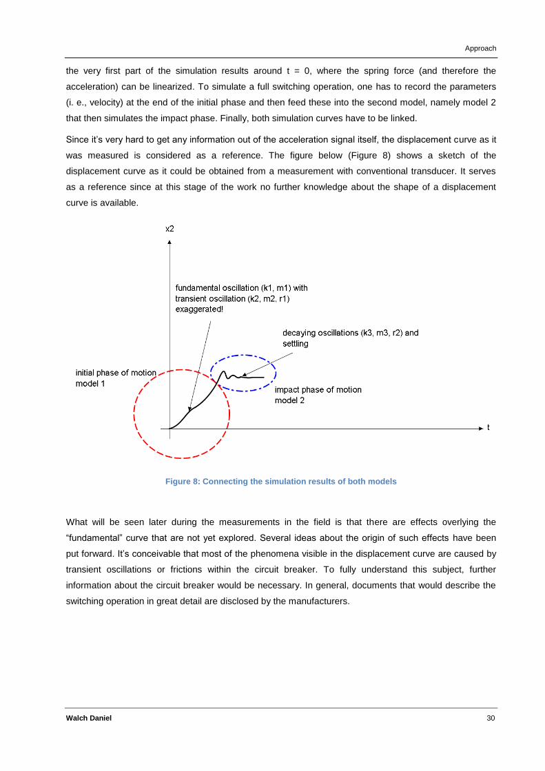
Since it’s very hard to get any information out of the acceleration signal itself, the displacement curve as it
was measured is considered as a reference. The figure below (Figure 8) shows a sketch of the
displacement curve as it could be obtained from a measurement with conventional transducer. It serves
as a reference since at this stage of the work no further knowledge about the shape of a displacement
curve is available.
Figure 8: Connecting the simulation results of both models
What will be seen later during the measurements in the field is that there are effects overlying the
“fundamental” curve that are not yet explored. Several ideas about the origin of such effects have been
put forward. It’s conceivable that most of the phenomena visible in the displacement curve are caused by
transient oscillations or frictions within the circuit breaker. To fully understand this subject, further
information about the circuit breaker would be necessary. In general, documents that would describe the
switching operation in great detail are disclosed by the manufacturers.
Approach
Walch Daniel 31
6.1.1 Equations
The equations for the models are given below. These could be used to implement the models in software
like Matlab-Simulink etc.
6.1.1.1 Model 1:
In the equations above, m1 and m2 represent the masses depicted in Figure 7, Model 1. Ff1 and Ff2
represent the forces caused by the springs. Fd1 is the force caused by the damper. The positions of mass
m1 and m2, respectively, are noted represented by x1 and x2. After rearranging, the following expressions
can be obtained. The constants k1, k2 and d1 are the spring constants of the corresponding springs and
the damping constant of the damper d1, respectively.
( ) ( )
( ) ( )
6.1.1.2 Model 2:
In Figure 7, Model 2 the above quantities can be found, where m3 represents the mass to be decelerated,
and x3 being the position of the mass m3. Ff3 and Fd2 are again the forces caused by the spring and the
damper depicted in the figure and k3 and d2 the corresponding constants.
6.1.2 Parameterization
The challenge is to allocate meaningful values to the parameters given in the proposed differential
equations. Detailed data for the circuit breakers is rare and the data sheets do not contain much
information about the mechanical and physical properties (mass, transmission ratio, torsion, etc.). Hence,
what can be done is to “adjust” the simulation to fit the measured data. The goal is to reproduce the curve
obtained from real measurements with the simulation output. This is somewhat cumbersome and the
model is not suited to describe all the effects that can be seen in the final displacement curve. So,
assigning values to the parameters is not explicitly shown here. What is still interesting in this context is to
check if the assumption that the driving spring force is approximately constant during a switching

Approach
Walch Daniel 32
operation is true. A sanity check using real measurement data is done in chapter whereas an alternative
approach to invent a model is presented in section 8.2.
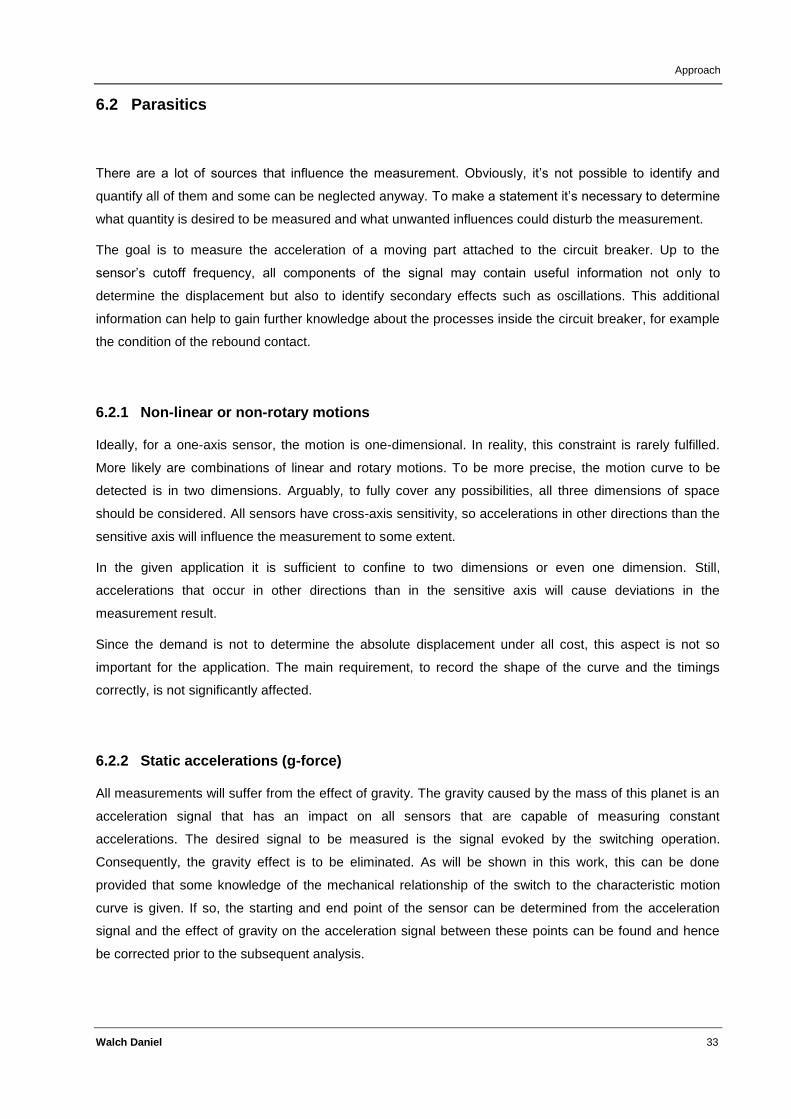
Approach
Walch Daniel 33
6.2 Parasitics
There are a lot of sources that influence the measurement. Obviously, it’s not possible to identify and
quantify all of them and some can be neglected anyway. To make a statement it’s necessary to determine
what quantity is desired to be measured and what unwanted influences could disturb the measurement.
The goal is to measure the acceleration of a moving part attached to the circuit breaker. Up to the
sensor’s cutoff frequency, all components of the signal may contain useful information not only to
determine the displacement but also to identify secondary effects such as oscillations. This additional
information can help to gain further knowledge about the processes inside the circuit breaker, for example
the condition of the rebound contact.
6.2.1 Non-linear or non-rotary motions
Ideally, for a one-axis sensor, the motion is one-dimensional. In reality, this constraint is rarely fulfilled.
More likely are combinations of linear and rotary motions. To be more precise, the motion curve to be
detected is in two dimensions. Arguably, to fully cover any possibilities, all three dimensions of space
should be considered. All sensors have cross-axis sensitivity, so accelerations in other directions than the
sensitive axis will influence the measurement to some extent.
In the given application it is sufficient to confine to two dimensions or even one dimension. Still,
accelerations that occur in other directions than in the sensitive axis will cause deviations in the
measurement result.
Since the demand is not to determine the absolute displacement under all cost, this aspect is not so
important for the application. The main requirement, to record the shape of the curve and the timings
correctly, is not significantly affected.
6.2.2 Static accelerations (g-force)
All measurements will suffer from the effect of gravity. The gravity caused by the mass of this planet is an
acceleration signal that has an impact on all sensors that are capable of measuring constant
accelerations. The desired signal to be measured is the signal evoked by the switching operation.
Consequently, the gravity effect is to be eliminated. As will be shown in this work, this can be done
provided that some knowledge of the mechanical relationship of the switch to the characteristic motion
curve is given. If so, the starting and end point of the sensor can be determined from the acceleration
signal and the effect of gravity on the acceleration signal between these points can be found and hence
be corrected prior to the subsequent analysis.
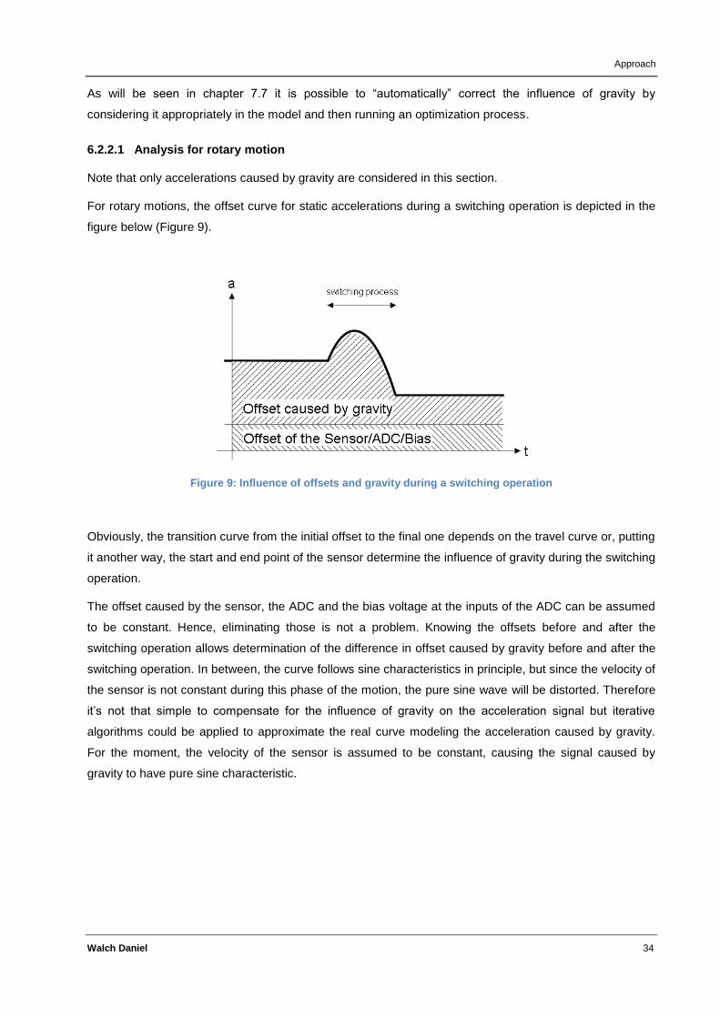
Approach
Walch Daniel 34
As will be seen in chapter 7.7 it is possible to “automatically” correct the influence of gravity by
considering it appropriately in the model and then running an optimization process.
6.2.2.1 Analysis for rotary motion
Note that only accelerations caused by gravity are considered in this section.
For rotary motions, the offset curve for static accelerations during a switching operation is depicted in the
figure below (Figure 9).
Figure 9: Influence of offsets and gravity during a switching operation
Obviously, the transition curve from the initial offset to the final one depends on the travel curve or, putting
it another way, the start and end point of the sensor determine the influence of gravity during the switching
operation.
The offset caused by the sensor, the ADC and the bias voltage at the inputs of the ADC can be assumed
to be constant. Hence, eliminating those is not a problem. Knowing the offsets before and after the
switching operation allows determination of the difference in offset caused by gravity before and after the
switching operation. In between, the curve follows sine characteristics in principle, but since the velocity of
the sensor is not constant during this phase of the motion, the pure sine wave will be distorted. Therefore
it’s not that simple to compensate for the influence of gravity on the acceleration signal but iterative
algorithms could be applied to approximate the real curve modeling the acceleration caused by gravity.
For the moment, the velocity of the sensor is assumed to be constant, causing the signal caused by
gravity to have pure sine characteristic.

Approach
Walch Daniel 35
Figure 10: Trigonometric relations at the sensor
a1 Acceleration measured in position 1 (Position before the switching operation)
a2 Acceleration measured in position 2 (Position after the switching operation)
φ1 Angle of lever to perpendicular in position 1
φ2 Angle of lever to perpendicular in position 2
Δφ Angle difference between position 1 and position 2 (φ1 – φ2)
g g-force (gravity)
aoff All (static) offsets caused by sensor offset, ADC offset, and bias voltage at the ADC input
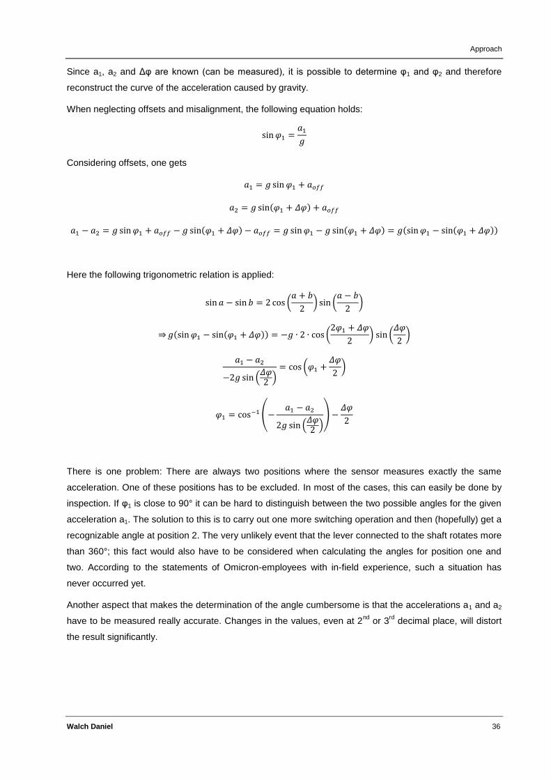
Approach
Walch Daniel 36
Since a1, a2 and Δφ are known (can be measured), it is possible to determine φ1 and φ2 and therefore
reconstruct the curve of the acceleration caused by gravity.
When neglecting offsets and misalignment, the following equation holds:
Considering offsets, one gets
( )
( ) ( ) ( ( ))
Here the following trigonometric relation is applied:
(
) (
)
⇒ ( ( )) (
) (
)
( ) (
)
(
( ))
There is one problem: There are always two positions where the sensor measures exactly the same
acceleration. One of these positions has to be excluded. In most of the cases, this can easily be done by
inspection. If φ1 is close to 90° it can be hard to distinguish between the two possible angles for the given
acceleration a1. The solution to this is to carry out one more switching operation and then (hopefully) get a
recognizable angle at position 2. The very unlikely event that the lever connected to the shaft rotates more
than 360°; this fact would also have to be considered when calculating the angles for position one and
two. According to the statements of Omicron-employees with in-field experience, such a situation has
never occurred yet.
Another aspect that makes the determination of the angle cumbersome is that the accelerations a1 and a2
have to be measured really accurate. Changes in the values, even at 2nd
or 3rd
decimal place, will distort
the result significantly.
Approach
Walch Daniel 37
Figure 11: Two equivalent sensor positions.
Obviously, for the example given above, the sensor will measure the same static acceleration such that a1
= a2.
Approach
Walch Daniel 38
As stated above, correcting this influence of gravity isn’t that easy since the pure trigonometric function
will be distorted due to the varying velocity of the sensor during the motion. When correcting the influence
of gravity on the measurement in practice, one would compensate the acceleration curve with an “initial
guess” of the influence of gravity and calculate the displacement. Then, this initial guess would be
improved iteratively by observing a certain measure that evaluates the quality of the displacement curve
(shape, drifts, etc.) until no further change in this quality measure function is present.
At least, it’s typically possible to determine the initial and final angle of the sensor’s sensitive axis and
therefore an estimate of the transition curve caused by gravity.
6.2.3 Temperature
The effect of temperature changes have not been investigated intensely. In general, the temperature of
the sensor may influence both offset and sensitivity. Temperature changes during a switching operation
may arise from changing solar radiation (sensor moves from a shadily position into the sun during
switching, for example) or changing wind conditions (even the air flow around the sensor during switching
might have an effect). Since the changes in temperature can be assumed to be low due to the comparably
short measurement time and since the sensors are not very vulnerable to temperature changes it’s
supposed that the influence of temperature on the measurement can be neglected.
What might be worth considering is the change of temperature from one measurement to another.
Comprehensibly, if one measurement takes place on a hot summer day and another one on a rainy
autumn day, the absolute signals out of the sensor will be different since certain characteristics such as
sensitivity change. As an example, one of the sensors used within this thesis (KS94B10) has a
temperature coefficient of the sensitivity of 0.05 %/K between -20 °C and 20 °C.
6.2.4 Mechanical stress
During a switching operation the sensors suffer from mechanical stress that might influence the
measurement system inside the sensor’s housing. This effect can hardly be comprehended but tried to be
avoided by following the mounting instructions given in the manuals.
Another phenomenon that affects the sensor is stress of the base of the sensor, referred to as base strain
sensitivity. When the base of the sensor is stressed also the measuring system within the case is affected.
An erroneous acceleration signal can be detected at the output of the sensor. It is caused for example by
bending, torque or distortion [58].
Other effects caused by mechanical stress are oscillations and vibrations. These will overlay the “original”
acceleration signal and influence the displacement curve. If identified properly, extraction of these
frequency components and further evaluation might help to gain additional knowledge about the circuit
breaker.
Approach
Walch Daniel 39
As an example, the oscillations that occur when the contacts hit the rebound contact can be used to say
something about the condition of the contacts.
Of course, oscillations of the housing of the circuit breaker and the like are not desired in the acceleration
signal and should be treated properly when processing the signal.
6.2.5 Noise
All real electronic components produce noise and so does the accelerometer. Usually, the noise density
and/or the residual noise as an RMS value are given in the sensor’s datasheet. From this information, the
influence on the measurement can be determined. Since DC accelerations and offsets are eliminated
from the acceleration signal in the processing step and integration is carried out twice, the noise issue will
not be of big concern, see the considerations below. Note that a statistical estimation of the maximum
allowed noise is a complex issue. To do so, an integration of a stochastic quantity has to be performed; it
comes to stochastic integrals and the related mathematics (Brownian motion, etc.). This would allow
estimations on the expected deviation of the displacement or, in other words, to ensure the displacement
stays within certain boundaries with a given probability. To avoid complex mathematics, estimations about
the maximum acceptable noise can be done using the example below.
6.2.5.1 Example
For the moment, let’s assume the acceleration signal consists only of noise. To simplify further, the noise
is assumed to be constant. Obviously, this disagrees with the definition of noise, but that’s not of concern
for this example.
( )
If the acceleration signal is constant, the velocity will be a linear function with time:
( ) ∫
The displacement signal is the integral of the velocity:
( ) ∫
Now, let’s limit the deviation in the displacement signal caused by a constant acceleration with 5 mm and
the duration of a switching operation with 50 ms. Then the maximum constant acceleration can be
determined:
( ) ∫ ∫
⇒
Often, the RMS value of the noise is given in the datasheet. Alternatively, it’s possible to estimate the
RMS noise by using the noise densities, see the paragraphs below.
Approach
Walch Daniel 40
The KS94B10 that is often used within this work has a RMS noise of typically 3 mg from 0.5 Hz to 20000
Hz. Assuming the extremely unlikely case that the sensor’s RMS noise during the measurement was a
constant, this constant value could be approximately 70 times higher than the RMS value given in the
datasheet without significantly affecting the displacement result. Even for the ADXL001 that is producing
significantly higher noise the assumed constant noise could be two times the RMS value of 105 mg
without affecting the displacement signal more than 5 mm. These examples show that the sensor noise is
not a critical issue.
Another method to estimate the deviation in the displacement signal originating from noise in the
acceleration signal is to consider the sampled data as realizations of a stochastic process. Due to the
process' characteristics it can be assumed that the samples are uncorrelated and independent. Since
integration corresponds to summation in the digital domain, a sum of realizations of a stochastic process
has to be considered. The expected value of this sum will be zero since the mean of the realizations is
zero. The standard deviation of a sum is the geometric sum of the standard deviation of the samples;
hence it increases with the number of addends. Knowing the standard deviation, the maximum "error" in
the velocity signal can be estimated. Reapplying this procedure, the corresponding quantities for the
displacement signal can be estimated.
Now, the discussion is continued with some general considerations about noise.
In datasheets, the noise density is often given in √ ⁄ or ⁄ and is referred to as Acceleration
Spectral Density (ASD). Some intuitive explanations on this topic are given in [59].
It’s important to know that noise, given in equivalent g portions, is often a RMS value. Sometimes this
detail is omitted in data sheets. For special waveforms such as sinusoidal or triangular waveforms the
relation between RMS and peak value is simple. For noise, the relation is a bit more complicated.
Noise is a random process that cannot be predicted. It can be described using statistical measures such
as expected value (“mean”) and variance (corresponds to the power of the signal if the expected value is
zero).
To say the noise is “white” is an assumption that often holds in practice. In this context one often speaks
of AWGN (Additive White Gaussian Noise), where the noise that is added to the signal is both white and
Gaussian. White noise has a flat power spectral density. This means that all frequency components
contain the same power (on average). The amplitude distribution of white noise can be assumed to be
Gaussian in this application.

Approach
Walch Daniel 41
Figure 12: Amplitude distribution of AWGN (Additive White Gaussian Noise).
The RMS value of a normally distributed random variable is the standard deviation σ. Since approximately
99.7% of the time the noise amplitude is within the interval from +/- 3σ we can assume the peak value of
white noise to be around three times higher than the RMS value. Obviously, it will be smaller most of the
time.
Typically, we can assume that the peak value is three to four times the RMS value [60].
Unfortunately, the ASD is a not a flat function but changes with frequency. Manufacturers often state the
ASDs at given frequencies and the “overall” RMS noise in a specified bandwidth. Not specifying the
bandwidth makes the RMS noise value meaningless.
Using the RMS or peak value of the noise it’s possible to estimate the worst case drift in the displacement
signal caused by noise in the acceleration signal. This worst case scenario is extremely unlikely to
happen. Still, if it would happen, the influence of the noise on the final displacement signal can be omitted.
6.2.5.2 Noise and ADC resolution
In order to compare the noise amplitudes to the quantization interval of an ADC qualitatively, one can use
the ASD or the RMS value of the sensor noise and calculate the “peak” value. If this peak value is
significantly higher than the quantization interval, the least significant bits are “wasted” and the effective
resolution of the ADC decreases. On the other hand, if the peak value is well below the quantization
interval, the influence of the noise on the measurement will not be detected at all.

Approach
Walch Daniel 42
The quantization interval of a symmetric bipolar ADC is
Vmax maximum input voltage
b resolution in bits
The residual noise is often given in multiples of the g-force. The sensitivity of the sensor is also given in
relation to the g-force as V/g if the sensor has a voltage output.
The peak value is calculated as
NRMS,g Residual noise RMS in multiples of g
S Sensitivity in V/g
M Multiplication factor
The multiplication factor can be chosen according to the reasoning given above, typically around 3.
Example
Vmax = 2.5 V
b = 16
M = 3
NRMS,g = 3000 µg
S = 10 mV/g
From this example for the KS94B10 used later on in the practical part of this thesis it can be seen that the
choosing a 16 bit ADC was an appropriate decision. Assuming that the noise of the ADC itself does not
exceed ½ LSB and other noise sources are neglected it can be said that the sensor noise will maximally
distort 1 bit of the ADC.
Approach
Walch Daniel 43
6.2.6 Sensor weight (mass)
In general CBs are much heavier and bigger than the sensor itself. Thus, attaching the sensor to a moving
part of the CB will not measurably influence the measurement since the additional weight can be
neglected. Sensor weight might be an issue when applying big and possibly heavy measurement
equipment to the CB. This case should never occur, even when mounting comparatively big and heavy
conventional sensors to the DUT this should not have a significant impact on the test series. It’s worth
mentioning that the sensor’s weight should be kept as low as possible due to the fact that mounting effort
increases with sensor weight.
6.2.7 Measurement equipment and AD conversion
All the measurement equipment attached to the sensor also introduces noise and makes the overall
measurement system more sensitive to external disturbing sources like electromagnetic fields. This effect
is antagonized by keeping the output impedance low or using current source characteristics. The AD
conversion part is a load to the sensor and must keep certain constraints. Sampling with a sampling
frequency that is too low and/or not using sufficient anti-aliasing filters will cause aliasing and loss of high-
frequency components that might be interesting to investigate. The place where the sensor is mounted
might well be at some distance to the AD conversion part what makes long cables necessary. The longer
the cable is, the higher the capacitive load to the sensor will be and the vulnerability to electromagnetic
influences will also increase.
As was found out empirically, these effects do not play an important role in the measurement system.
Anyway, it’s always a good thing to use properly shielded and guarded cables and apply well-known
techniques (i. e. differential signaling) to keep the influence of the measurement equipment on the actual
measurement low.
6.2.8 Mounting
In order to record all measurable frequency components a very inflexible connection between sensor and
device under test has to be achieved. Moreover, (severe) manipulations of the mechanical parts the
sensor is attached to are not desired.
Commonly used mounting methods are adhesive bonding and stud mounting. Adhesives are available in
many different forms. Practical experiences have shown that “standard” super glues are sufficient for the
application [61]. The mounting method will affect the frequency characteristics of the measurement
system, in particular the mounted natural frequency. Unfortunately it’s hard or even impossible to
determine the exact frequency characteristics of a given adhesive bond. Some estimates can be found in
the literature, for example on the website of The Modal Shop, Inc., see Figure 13 [62]. Of course, not only
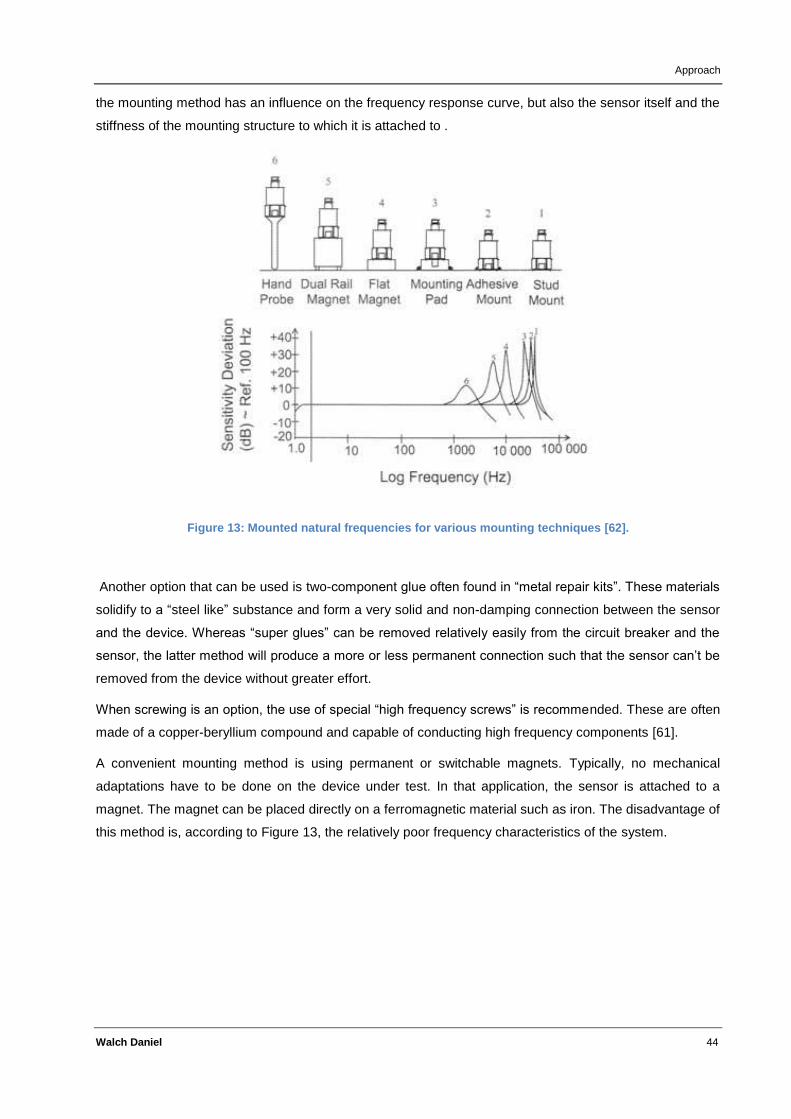
Approach
Walch Daniel 44
the mounting method has an influence on the frequency response curve, but also the sensor itself and the
stiffness of the mounting structure to which it is attached to .
Figure 13: Mounted natural frequencies for various mounting techniques [62].
Another option that can be used is two-component glue often found in “metal repair kits”. These materials
solidify to a “steel like” substance and form a very solid and non-damping connection between the sensor
and the device. Whereas “super glues” can be removed relatively easily from the circuit breaker and the
sensor, the latter method will produce a more or less permanent connection such that the sensor can’t be
removed from the device without greater effort.
When screwing is an option, the use of special “high frequency screws” is recommended. These are often
made of a copper-beryllium compound and capable of conducting high frequency components [61].
A convenient mounting method is using permanent or switchable magnets. Typically, no mechanical
adaptations have to be done on the device under test. In that application, the sensor is attached to a
magnet. The magnet can be placed directly on a ferromagnetic material such as iron. The disadvantage of
this method is, according to Figure 13, the relatively poor frequency characteristics of the system.
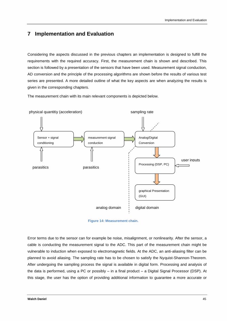
Implementation and Evaluation
Walch Daniel 45
7 Implementation and Evaluation
Considering the aspects discussed in the previous chapters an implementation is designed to fulfill the
requirements with the required accuracy. First, the measurement chain is shown and described. This
section is followed by a presentation of the sensors that have been used. Measurement signal conduction,
AD conversion and the principle of the processing algorithms are shown before the results of various test
series are presented. A more detailed outline of what the key aspects are when analyzing the results is
given in the corresponding chapters.
The measurement chain with its main relevant components is depicted below.
Error terms due to the sensor can for example be noise, misalignment, or nonlinearity. After the sensor, a
cable is conducting the measurement signal to the ADC. This part of the measurement chain might be
vulnerable to induction when exposed to electromagnetic fields. At the ADC, an anti-aliasing filter can be
planned to avoid aliasing. The sampling rate has to be chosen to satisfy the Nyquist-Shannon-Theorem.
After undergoing the sampling process the signal is available in digital form. Processing and analysis of
the data is performed, using a PC or possibly – in a final product – a Digital Signal Processor (DSP). At
this stage, the user has the option of providing additional information to guarantee a more accurate or
Sensor + signal
conditioning
measurement signal
conduction
Analog/Digital
Conversion
physical quantitiy (acceleration)
parasitics parasitics Processing (DSP, PC)
sampling rate
graphical Presentation
(GUI)
analog domain digital domain
user inputs
Figure 14: Measurement chain.
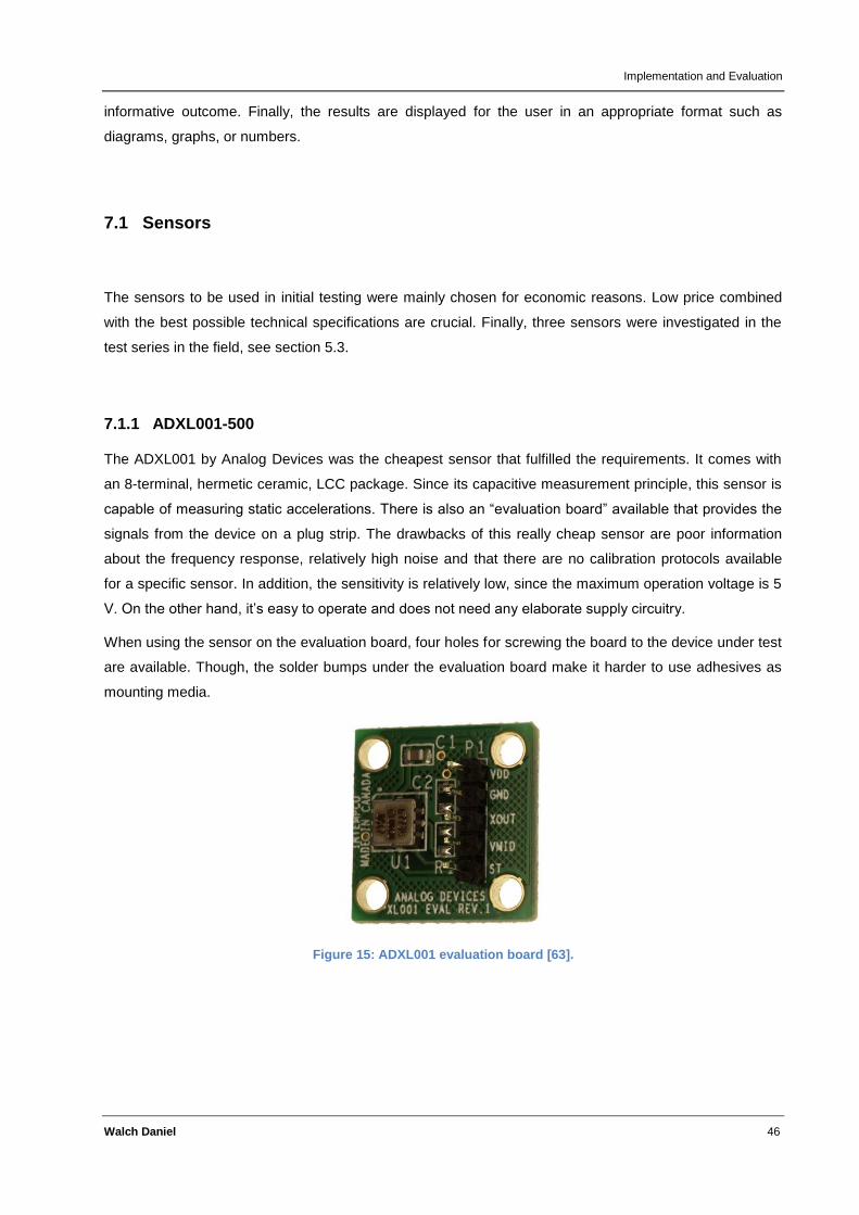
Implementation and Evaluation
Walch Daniel 46
informative outcome. Finally, the results are displayed for the user in an appropriate format such as
diagrams, graphs, or numbers.
7.1 Sensors
The sensors to be used in initial testing were mainly chosen for economic reasons. Low price combined
with the best possible technical specifications are crucial. Finally, three sensors were investigated in the
test series in the field, see section 5.3.
7.1.1 ADXL001-500
The ADXL001 by Analog Devices was the cheapest sensor that fulfilled the requirements. It comes with
an 8-terminal, hermetic ceramic, LCC package. Since its capacitive measurement principle, this sensor is
capable of measuring static accelerations. There is also an “evaluation board” available that provides the
signals from the device on a plug strip. The drawbacks of this really cheap sensor are poor information
about the frequency response, relatively high noise and that there are no calibration protocols available
for a specific sensor. In addition, the sensitivity is relatively low, since the maximum operation voltage is 5
V. On the other hand, it’s easy to operate and does not need any elaborate supply circuitry.
When using the sensor on the evaluation board, four holes for screwing the board to the device under test
are available. Though, the solder bumps under the evaluation board make it harder to use adhesives as
mounting media.
Figure 15: ADXL001 evaluation board [63].
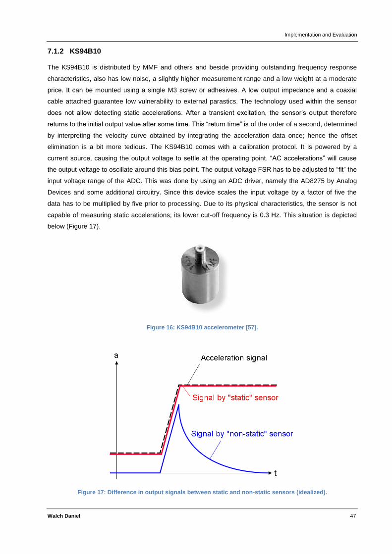
Implementation and Evaluation
Walch Daniel 47
7.1.2 KS94B10
The KS94B10 is distributed by MMF and others and beside providing outstanding frequency response
characteristics, also has low noise, a slightly higher measurement range and a low weight at a moderate
price. It can be mounted using a single M3 screw or adhesives. A low output impedance and a coaxial
cable attached guarantee low vulnerability to external parastics. The technology used within the sensor
does not allow detecting static accelerations. After a transient excitation, the sensor’s output therefore
returns to the initial output value after some time. This “return time” is of the order of a second, determined
by interpreting the velocity curve obtained by integrating the acceleration data once; hence the offset
elimination is a bit more tedious. The KS94B10 comes with a calibration protocol. It is powered by a
current source, causing the output voltage to settle at the operating point. “AC accelerations” will cause
the output voltage to oscillate around this bias point. The output voltage FSR has to be adjusted to “fit” the
input voltage range of the ADC. This was done by using an ADC driver, namely the AD8275 by Analog
Devices and some additional circuitry. Since this device scales the input voltage by a factor of five the
data has to be multiplied by five prior to processing. Due to its physical characteristics, the sensor is not
capable of measuring static accelerations; its lower cut-off frequency is 0.3 Hz. This situation is depicted
below (Figure 17).
Figure 16: KS94B10 accelerometer [57].
Figure 17: Difference in output signals between static and non-static sensors (idealized).
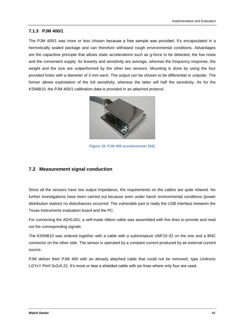
Implementation and Evaluation
Walch Daniel 48
7.1.3 PJM 400/1
The PJM 400/1 was more or less chosen because a free sample was provided. It’s encapsulated in a
hermetically sealed package and can therefore withstand rough environmental conditions. Advantages
are the capacitive principle that allows static accelerations such as g-force to be detected, the low noise
and the convenient supply. Its linearity and sensitivity are average, whereas the frequency response, the
weight and the size are outperformed by the other two sensors. Mounting is done by using the four
provided holes with a diameter of 3 mm each. The output can be chosen to be differential or unipolar. The
former allows exploitation of the full sensitivity, whereas the latter will half the sensitivity. As for the
KS94B10, the PJM 400/1 calibration data is provided in an attached protocol.
Figure 18: PJM 400 accelerometer [64].
7.2 Measurement signal conduction
Since all the sensors have low output impedance, the requirements on the cables are quite relaxed. No
further investigations have been carried out because even under harsh environmental conditions (power
distribution station) no disturbances occurred. The vulnerable part is really the USB interface between the
Texas Instruments evaluation board and the PC.
For connecting the ADXL001, a self-made ribbon cable was assembled with five lines to provide and read
out the corresponding signals.
The KS94B10 was ordered together with a cable with a subminiature UNF10-32 on the one and a BNC
connector on the other side. The sensor is operated by a constant current produced by an external current
source.
PJM deliver their PJM 400 with an already attached cable that could not be removed, type Unitronic
Li2YcY Pimf 3x2x0.22. It’s more or less a shielded cable with six lines where only four are used.

Implementation and Evaluation
Walch Daniel 49
7.3 Analog-Digital-Conversion
In order to further process the data gathered by the sensors, an AD conversion has to be performed. The
requirements to consider for the Analog-to-Digital-Converter (ADC) are its bandwidth, resolution and
linearity since (static) offset errors can be compensated and are not an issue. The cut-off frequency of the
sensors is around 10 kHz, hence choosing a sampling frequency of around 20 kHz is sufficient, but 40
kHz is better. From the example in section 6.2.5.2 it’s known that a resolution of 16 bit satisfies the
requirements. Within the context of this thesis no excessive studies concerning the choice of ADCs has
been carried out. Since already available at the supporting company the decision was made in favor of the
ADS1174 or ADS1274, respectively, both by Texas Instruments where the ADS1274 model is the more
advanced one. The ADCs are so called ΔΣ-converters with the main advantages that “noise forming” can
be applied and there is no explicit sample and hold stage necessary since continuous sampling at the
ADC inputs is performed. Moreover, 64-times oversampling is implemented, making anti-aliasing filters
unnecessary or at least relaxing the requirements for the filter. In order to keep the expenditure of time
low, no circuitry with the ADC was developed but the evaluation boards ADS1174EVM-PDK and
ADS1274EVM-PDK with the MMB0 “motherboard” were used.
Figure 19: ADS1274EVM-PDK ADC evaluation board [65].
7.4 Processing
At this stage of the work, a “normal” PC is used to analyze the data. Matlab is used to do all calculations
and present the results in graphical form.
In a final product, the usage of a DSP can be an option, depending on the overall measurement
equipment. If a PC is necessary to display the displacement curves, the use of a dedicated DSP for
performing calculations will most probably not be required since the PC would be capable of performing
all necessary calculations.
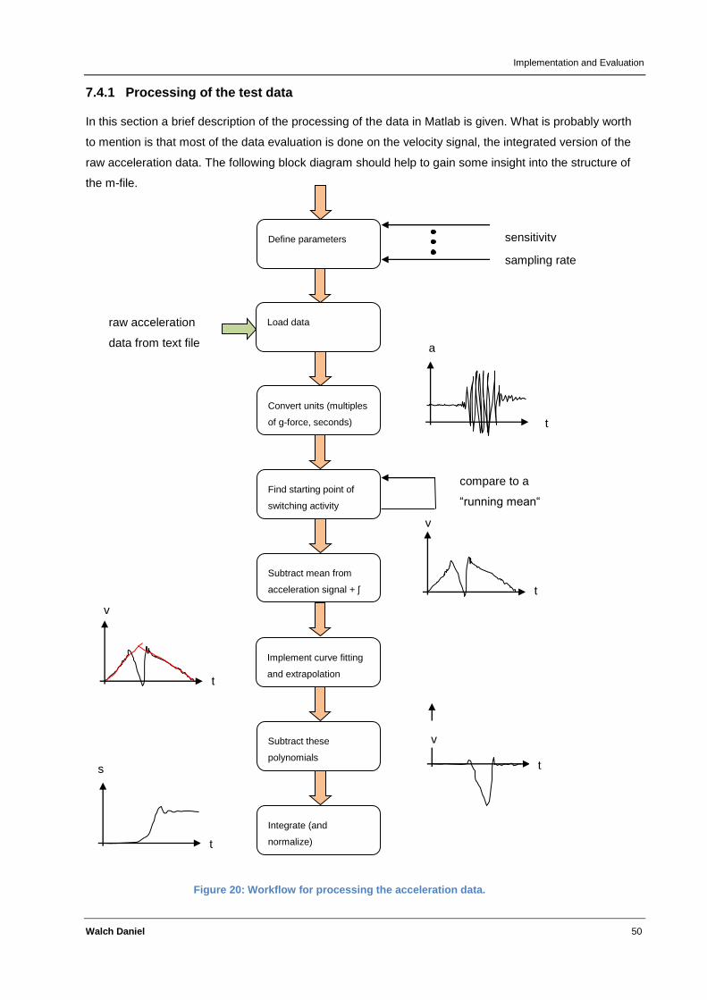
Implementation and Evaluation
Walch Daniel 50
7.4.1 Processing of the test data
In this section a brief description of the processing of the data in Matlab is given. What is probably worth
to mention is that most of the data evaluation is done on the velocity signal, the integrated version of the
raw acceleration data. The following block diagram should help to gain some insight into the structure of
the m-file.
Define parameters sensitivity
sampling rate
Load data raw acceleration
data from text file
Convert units (multiples
of g-force, seconds)
Find starting point of
switching activity
compare to a
“running mean“
Subtract mean from
acceleration signal + ʃ
a
t
Implement curve fitting
and extrapolation
v
t
Subtract these
polynomials
v
t
v
t
Integrate (and
normalize)
s
t
Figure 20: Workflow for processing the acceleration data.

Implementation and Evaluation
Walch Daniel 51
Some aspects have to be noted concerning the processing of the acceleration data. A lot of the
parameters (degree of curve fitting polynomials, estimated length of the switching operation, etc.) that
affect the processing of the acceleration data are adjusted manually right now. Of course, the choice of
these parameters will influence the result, namely the displacement curve. By careful assigning of values
to the parameters the results will improve. The challenge is not to manipulate the results of the
measurement by “tuning” the values such that the result is satisfying. This is not easy because it’s hard to
evaluate if by varying one of the parameters whether the processing algorithm itself improves or just the
results were “artificially” made better.
At a later stage of the project the determination of the parameters should be automated as far as
practicable to avoid such potentially confusing influences on the processing algorithms.
7.5 Graphical presentation
When using a PC for processing, obviously its screen is used for the graphical presentation of the results.
Since the shape of the curve in the time domain is crucial, a display that is capable of displaying such a
curve with acceptable accuracy is necessary. This has to be considered when thinking about “stand-
alone” measurement equipment that operates without the use of a PC.
7.6 Test series
After setting up the measurement equipment, various tests have been carried out. The two test objects
that were available were an older design medium voltage circuit breaker located at Omicron and a newer
design high voltage circuit breaker by Areva, investigated during a test series in Werben in September
2010.
Due to its persistent availability, the medium voltage circuit breaker is used for many of the tests. In
addition, a “conventional” sensor (transducer) has been attached to it, namely a rotary sensor. This gives
the opportunity to measure the displacement with the conventional sensor and accelerometers at the
same time. A comparison can be drawn between the various techniques as well as between the results
from different accelerometers.
The components where the accelerometers are placed using screws, magnetic or adhesive mount were
levers or rods that undergo a rotary, linear or a combined rotary and linear motion in two dimensions. The
exact geometrical relations have not been studied extensively, still a “by hand” measurement with a ruler
was done to determine the approximate absolute displacement of the sensor. Since absolute information

Implementation and Evaluation
Walch Daniel 52
about the displacement is not a must have, at least the shape of the displacement curves should be
similar for all sensors and methods and can be investigated.
When discussing the results obtained from the test series, the primary focus will be answering or
commenting on the requirements given in chapter 2:
- Reproducibility – Do the results of consecutive measurements match?
- Accuracy – To what extent is it possible to determine the absolute displacement?
- Quality – How exactly does the shape of the final curve match the expected one?
- Attachment – What methods are suited best for attachment?
- Comparability – How does the new method compare to conventional ones?
In order to keep the evaluation neatly arranged, a number of potentially interesting aspects have been
chosen to be discussed. The subsequent chapters will each cover one of these aspects:
- Noise and drift considerations
- Obtaining a “reference curve” using the conventional transducer
- Comparing the results of the conventional transducer with the results obtained with
accelerometers
- Comparing various sampling rates and two ADC resolutions
- Comparing results of one and the same sensor
- Comparing the results of different accelerometer types
- Investigating the absolute displacement information with respect to accuracy
- Comparing different mounting techniques
After going through these analyses the results will be evaluated and discussed.
7.6.1 Noise and drift
Firstly, the output of the sensors at rest is observed. This provides some information about the noise of
the whole measurement system and possible (short-term) drifts.
A total number of nine measurements were used to determine the noise present at the ADC’s input. The
two quantities calculated are the maximum peak-to-peak voltage and the RMS-value of the acceleration
data sampled by the ADC, both in Volts.
The maximum peak-to-peak voltage is calculated as follows:
( ) ( )
With vvec being the acceleration data vector in Volts.
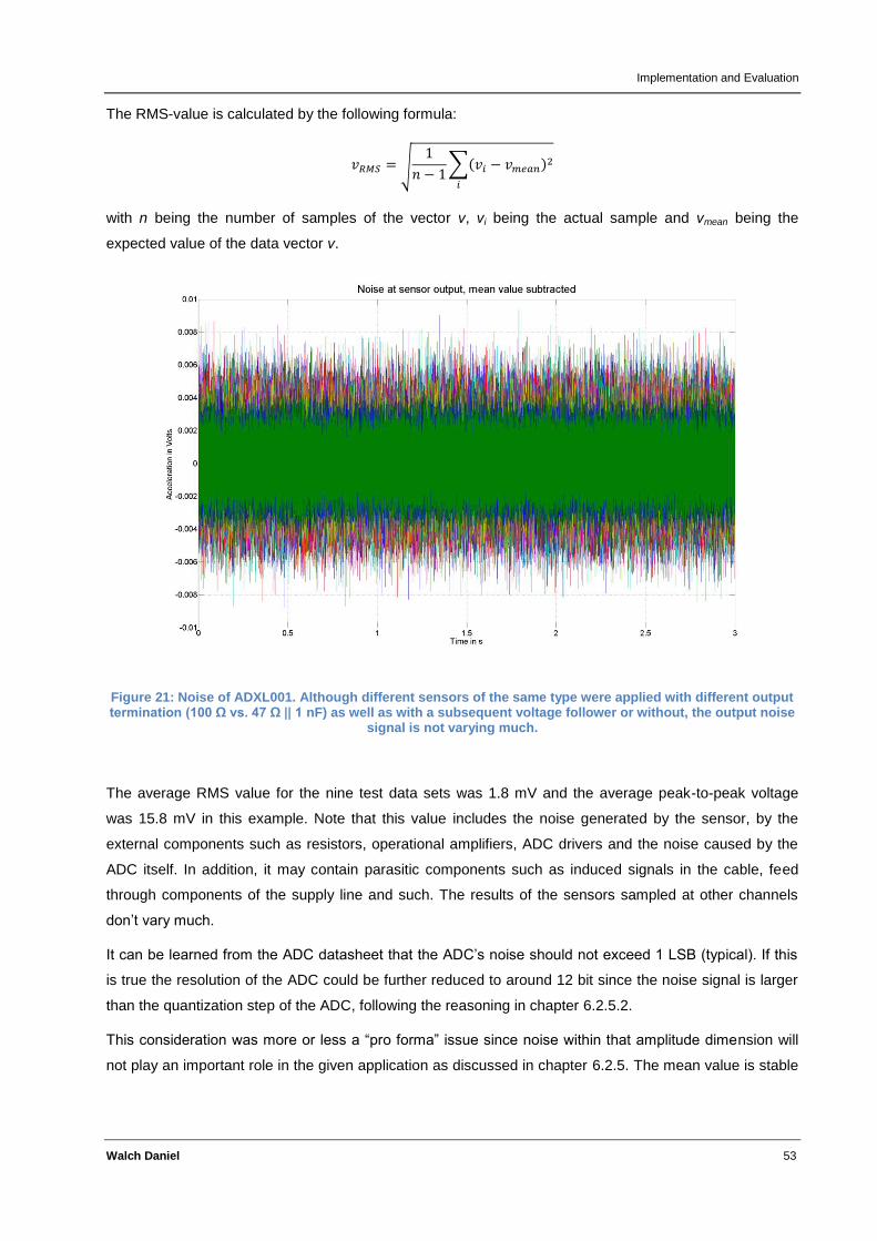
Implementation and Evaluation
Walch Daniel 53
The RMS-value is calculated by the following formula:
√
∑( )
with n being the number of samples of the vector v, vi being the actual sample and vmean being the
expected value of the data vector v.
Figure 21: Noise of ADXL001. Although different sensors of the same type were applied with different output termination (100 Ω vs. 47 Ω || 1 nF) as well as with a subsequent voltage follower or without, the output noise
signal is not varying much.
The average RMS value for the nine test data sets was 1.8 mV and the average peak-to-peak voltage
was 15.8 mV in this example. Note that this value includes the noise generated by the sensor, by the
external components such as resistors, operational amplifiers, ADC drivers and the noise caused by the
ADC itself. In addition, it may contain parasitic components such as induced signals in the cable, feed
through components of the supply line and such. The results of the sensors sampled at other channels
don’t vary much.
It can be learned from the ADC datasheet that the ADC’s noise should not exceed 1 LSB (typical). If this
is true the resolution of the ADC could be further reduced to around 12 bit since the noise signal is larger
than the quantization step of the ADC, following the reasoning in chapter 6.2.5.2.
This consideration was more or less a “pro forma” issue since noise within that amplitude dimension will
not play an important role in the given application as discussed in chapter 6.2.5. The mean value is stable
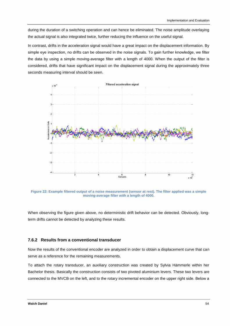
Implementation and Evaluation
Walch Daniel 54
during the duration of a switching operation and can hence be eliminated. The noise amplitude overlaying
the actual signal is also integrated twice, further reducing the influence on the useful signal.
In contrast, drifts in the acceleration signal would have a great impact on the displacement information. By
simple eye inspection, no drifts can be observed in the noise signals. To gain further knowledge, we filter
the data by using a simple moving-average filter with a length of 4000. When the output of the filter is
considered, drifts that have significant impact on the displacement signal during the approximately three
seconds measuring interval should be seen.
Figure 22: Example filtered output of a noise measurement (sensor at rest). The filter applied was a simple moving-average filter with a length of 4000.
When observing the figure given above, no deterministic drift behavior can be detected. Obviously, long-
term drifts cannot be detected by analyzing these results.
7.6.2 Results from a conventional transducer
Now the results of the conventional encoder are analyzed in order to obtain a displacement curve that can
serve as a reference for the remaining measurements.
To attach the rotary transducer, an auxiliary construction was created by Sylvia Hämmerle within her
Bachelor thesis. Basically the construction consists of two pivoted aluminium levers. These two levers are
connected to the MVCB on the left, and to the rotary incremental encoder on the upper right side. Below a
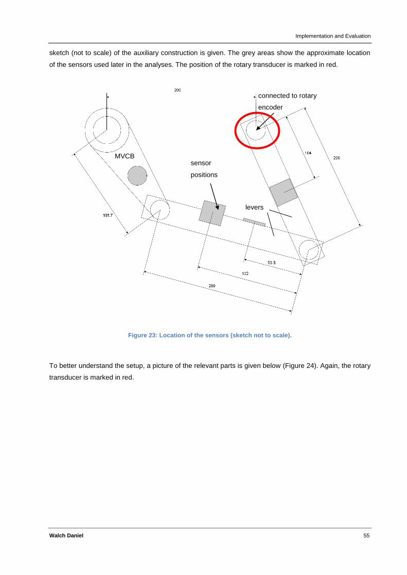
Implementation and Evaluation
Walch Daniel 55
sketch (not to scale) of the auxiliary construction is given. The grey areas show the approximate location
of the sensors used later in the analyses. The position of the rotary transducer is marked in red.
Figure 23: Location of the sensors (sketch not to scale).
To better understand the setup, a picture of the relevant parts is given below (Figure 24). Again, the rotary
transducer is marked in red.
MVCB
connected to rotary
encoder
sensor
positions
levers
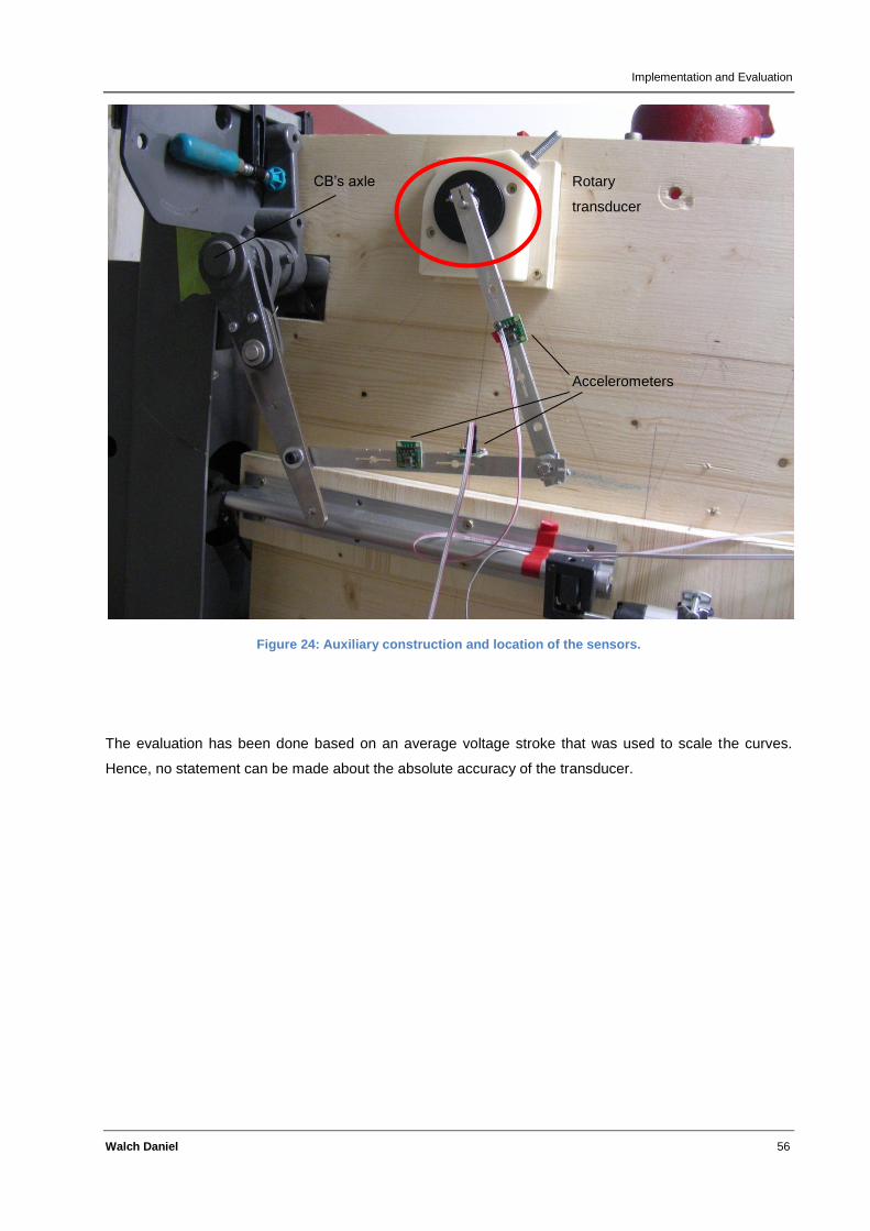
Implementation and Evaluation
Walch Daniel 56
Figure 24: Auxiliary construction and location of the sensors.
The evaluation has been done based on an average voltage stroke that was used to scale the curves.
Hence, no statement can be made about the absolute accuracy of the transducer.
Rotary
transducer
Accelerometers
CB’s axle
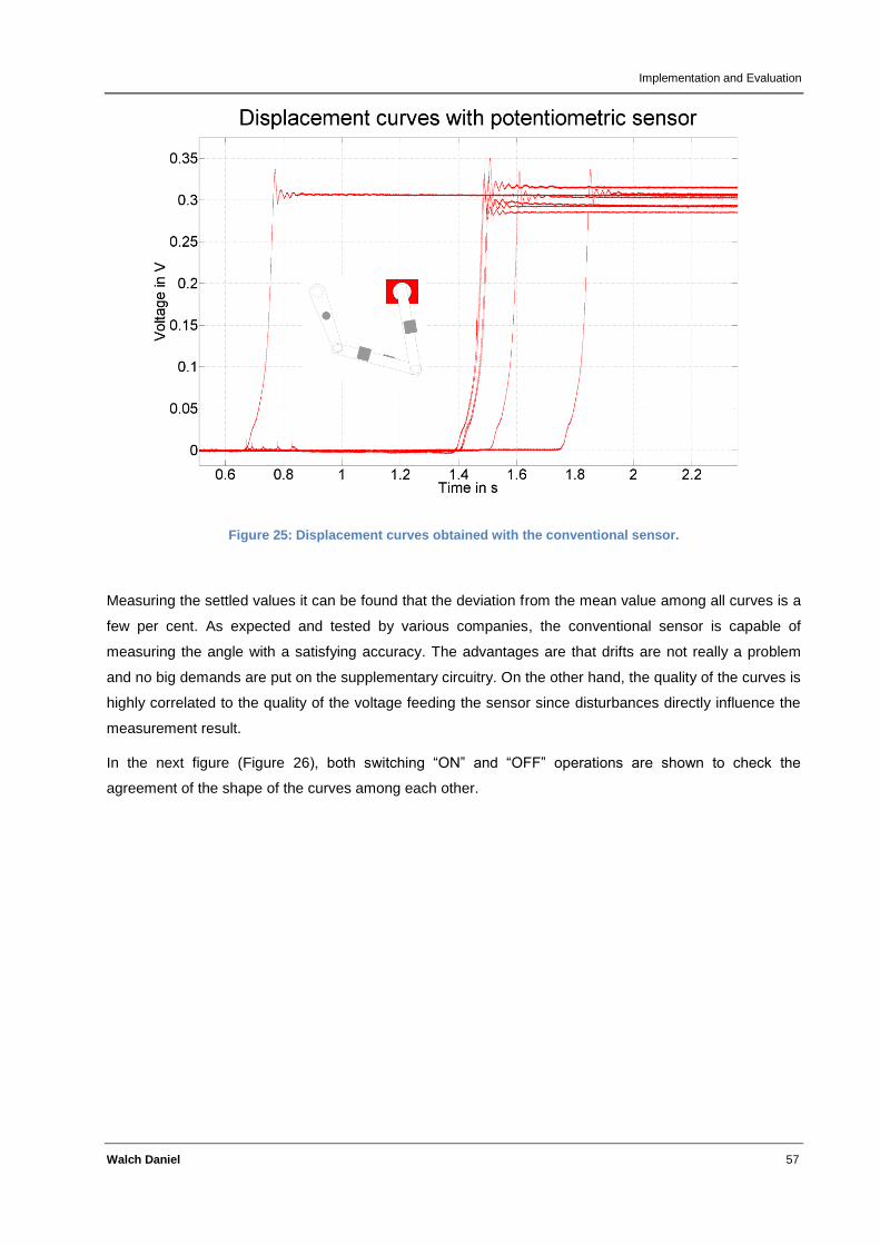
Implementation and Evaluation
Walch Daniel 57
Figure 25: Displacement curves obtained with the conventional sensor.
Measuring the settled values it can be found that the deviation from the mean value among all curves is a
few per cent. As expected and tested by various companies, the conventional sensor is capable of
measuring the angle with a satisfying accuracy. The advantages are that drifts are not really a problem
and no big demands are put on the supplementary circuitry. On the other hand, the quality of the curves is
highly correlated to the quality of the voltage feeding the sensor since disturbances directly influence the
measurement result.
In the next figure (Figure 26), both switching “ON” and “OFF” operations are shown to check the
agreement of the shape of the curves among each other.
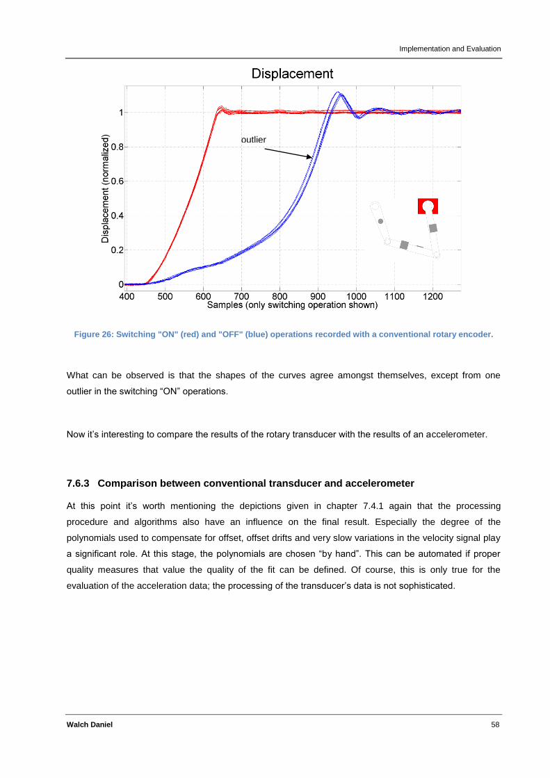
Implementation and Evaluation
Walch Daniel 58
Figure 26: Switching "ON" (red) and "OFF" (blue) operations recorded with a conventional rotary encoder.
What can be observed is that the shapes of the curves agree amongst themselves, except from one
outlier in the switching “ON” operations.
Now it’s interesting to compare the results of the rotary transducer with the results of an accelerometer.
7.6.3 Comparison between conventional transducer and accelerometer
At this point it’s worth mentioning the depictions given in chapter 7.4.1 again that the processing
procedure and algorithms also have an influence on the final result. Especially the degree of the
polynomials used to compensate for offset, offset drifts and very slow variations in the velocity signal play
a significant role. At this stage, the polynomials are chosen “by hand”. This can be automated if proper
quality measures that value the quality of the fit can be defined. Of course, this is only true for the
evaluation of the acceleration data; the processing of the transducer’s data is not sophisticated.
outlier
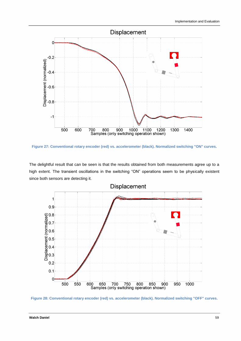
Implementation and Evaluation
Walch Daniel 59
Figure 27: Conventional rotary encoder (red) vs. accelerometer (black). Normalized switching "ON" curves.
The delightful result that can be seen is that the results obtained from both measurements agree up to a
high extent. The transient oscillations in the switching “ON” operations seem to be physically existent
since both sensors are detecting it.
Figure 28: Conventional rotary encoder (red) vs. accelerometer (black). Normalized switching "OFF" curves.

Implementation and Evaluation
Walch Daniel 60
This last finding is a very important one since it answers the question whether or not the new, innovative
method of measuring the displacement of the contacts of a CB is competitive with the conventional
method. From the preceding figures it’s safe to state that using accelerometers in the given application is
a more than appropriate alternative option to fulfill the requirements that are given in chapter 2.1.
7.6.4 Comparison of subsequent measurements with the same sensor
The reproducibility of the results of one and the same sensor is investigated. The sensor that was used is
the one described in chapter 7.6.1.1, mounted using two-component epoxy glue.
The ADXL001 sensor was glued onto a small print together with a voltage follower in order to decouple
the accelerometer’s output from the cable (capacitive load) and the ADC inputs. The print where the
sensor and the impedance converter are located on was attached to a lever of the medium voltage circuit
breaker using “Epoxy two-component glue” that produces a pretty stiff, hard-to-detach connection to the
DUT. According to first rough estimates, the resulting mechanical bond, due to its stiffness, should be
capable of conducting also high frequency accelerations from the lever to the sensor. Unfortunately, the
hot glue connecting the sensor to the board is not best suited for conducting high frequency components.
This statement is an estimate since there are no relevant studies about the frequency characteristics of
adhesive mounting methods around. Hence, the overall frequency response of the mechanical system is
most probably limited by the connection of the sensor onto the print. See Figure 29 for a picture of the
mounted sensor.
As mentioned, the drawback of this mounting method is that it’s hard to detach the board with the sensor
and impedance follower circuitry from the medium voltage circuit breaker lever.
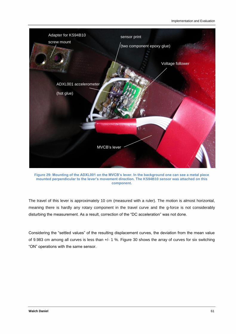
Implementation and Evaluation
Walch Daniel 61
Figure 29: Mounting of the ADXL001 on the MVCB’s lever. In the background one can see a metal piece mounted perpendicular to the lever’s movement direction. The KS94B10 sensor was attached on this
component.
The travel of this lever is approximately 10 cm (measured with a ruler). The motion is almost horizontal,
meaning there is hardly any rotary component in the travel curve and the g-force is not considerably
disturbing the measurement. As a result, correction of the “DC acceleration” was not done.
Considering the “settled values” of the resulting displacement curves, the deviation from the mean value
of 9.983 cm among all curves is less than +/- 1 %. Figure 30 shows the array of curves for six switching
“ON” operations with the same sensor.
Voltage follower
ADXL001 accelerometer
(hot glue)
sensor print
(two component epoxy glue)
MVCB’s lever
Adapter for KS94B10
screw mount
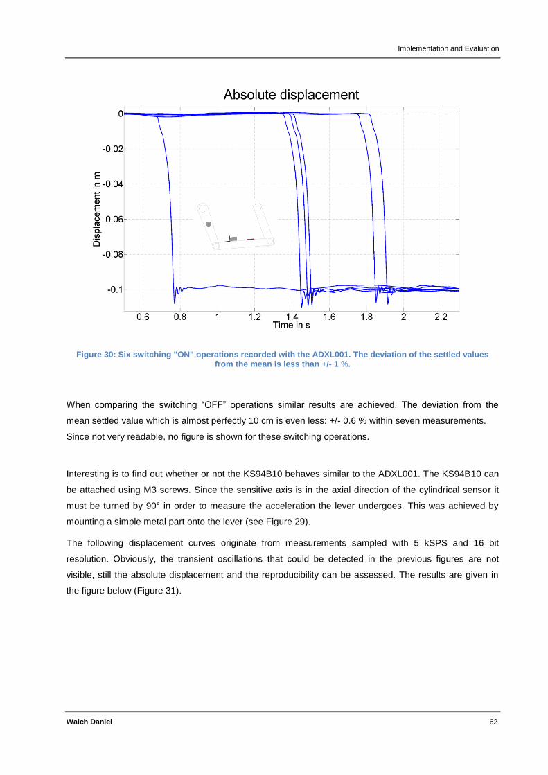
Implementation and Evaluation
Walch Daniel 62
Figure 30: Six switching "ON" operations recorded with the ADXL001. The deviation of the settled values from the mean is less than +/- 1 %.
When comparing the switching “OFF” operations similar results are achieved. The deviation from the
mean settled value which is almost perfectly 10 cm is even less: +/- 0.6 % within seven measurements.
Since not very readable, no figure is shown for these switching operations.
Interesting is to find out whether or not the KS94B10 behaves similar to the ADXL001. The KS94B10 can
be attached using M3 screws. Since the sensitive axis is in the axial direction of the cylindrical sensor it
must be turned by 90° in order to measure the acceleration the lever undergoes. This was achieved by
mounting a simple metal part onto the lever (see Figure 29).
The following displacement curves originate from measurements sampled with 5 kSPS and 16 bit
resolution. Obviously, the transient oscillations that could be detected in the previous figures are not
visible, still the absolute displacement and the reproducibility can be assessed. The results are given in
the figure below (Figure 31).
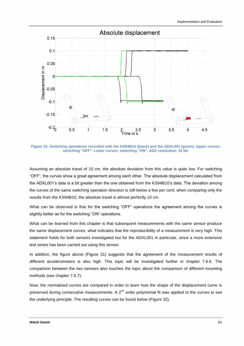
Implementation and Evaluation
Walch Daniel 63
Figure 31: Switching operations recorded with the KS94B10 (black) and the ADXL001 (green). Upper curves: switching "OFF". Lower curves: switching "ON". ADC resolution: 16 bit.
Assuming an absolute travel of 10 cm, the absolute deviation from this value is quite low. For switching
“OFF”, the curves show a great agreement among each other. The absolute displacement calculated from
the ADXL001’s data is a bit greater than the one obtained from the KS94B10’s data. The deviation among
the curves of the same switching operation direction is still below a few per cent; when comparing only the
results from the KS94B10, the absolute travel is almost perfectly 10 cm.
What can be observed is that for the switching “OFF” operations the agreement among the curves is
slightly better as for the switching “ON” operations.
What can be learned from this chapter is that subsequent measurements with the same sensor produce
the same displacement curves, what indicates that the reproducibility of a measurement is very high. This
statement holds for both sensors investigated but for the ADXL001 in particular, since a more extensive
test series has been carried out using this sensor.
In addition, the figure above (Figure 31) suggests that the agreement of the measurement results of
different accelerometers is also high. This topic will be investigated further in chapter 7.6.6. The
comparison between the two sensors also touches the topic about the comparison of different mounting
methods (see chapter 7.6.7).
Now, the normalized curves are compared in order to learn how the shape of the displacement curve is
preserved during consecutive measurements. A 2nd
order polynomial fit was applied to the curves to see
the underlying principle. The resulting curves can be found below (Figure 32).

Implementation and Evaluation
Walch Daniel 64
Figure 32: Normalized displacement curves. Upper curves: switching "OFF". Lower curves: switching "ON". Dashed lines: 2nd order polynomial fits.
It can be seen that the curves agree to a high extent. Obviously, both sensors output very similar
acceleration data, despite they use different measuring techniques. It’s worth mentioning that overshoot
and transient oscillations cannot be seen in the figure. The reason is not yet investigated thoroughly. An
assumption is that by integrating twice accompanied by smoothing these oscillations are filtered out. The
switching operations were sampled with 5 kSPS what seems not to be sufficient even though Shannon’s
sampling theorem seems to be satisfied. Anyway, I ncreasing the sample rate produces better
displacement curves, as can be seen in various chapters in this thesis.
This topic will be investigated in the next chapter (chapter 7.6.5).
An interesting aspect might be to look at the difference signal between the 2nd order polynomial fits and
the calculated displacement curve. The results are displayed below (
Figure 33).
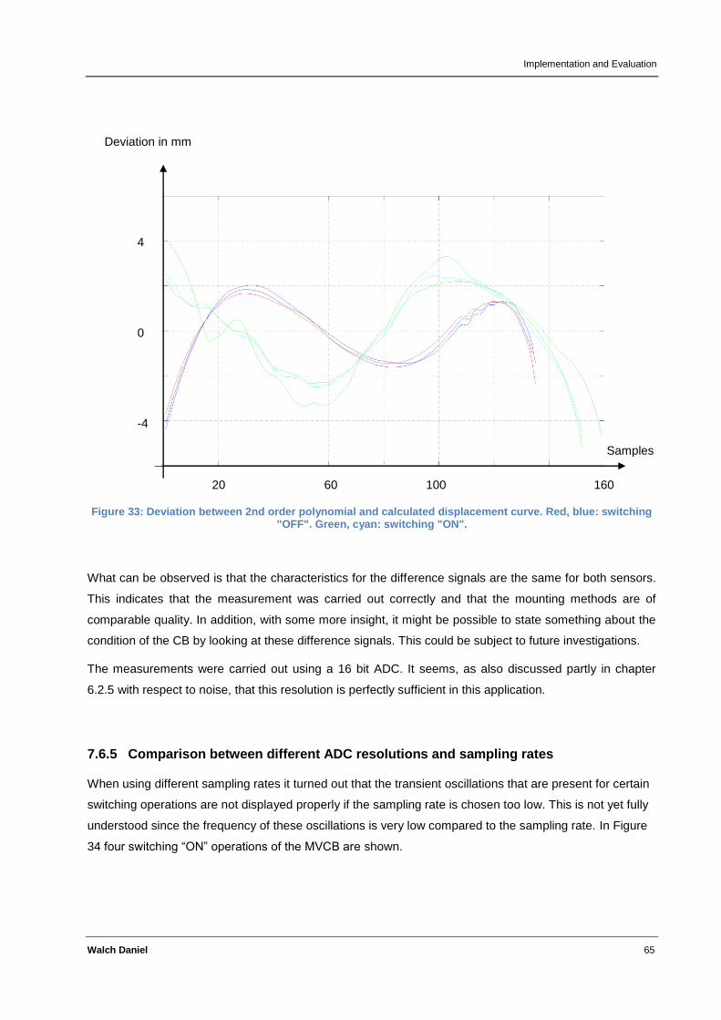
Implementation and Evaluation
Walch Daniel 65
Figure 33: Deviation between 2nd order polynomial and calculated displacement curve. Red, blue: switching "OFF". Green, cyan: switching "ON".
What can be observed is that the characteristics for the difference signals are the same for both sensors.
This indicates that the measurement was carried out correctly and that the mounting methods are of
comparable quality. In addition, with some more insight, it might be possible to state something about the
condition of the CB by looking at these difference signals. This could be subject to future investigations.
The measurements were carried out using a 16 bit ADC. It seems, as also discussed partly in chapter
6.2.5 with respect to noise, that this resolution is perfectly sufficient in this application.
7.6.5 Comparison between different ADC resolutions and sampling rates
When using different sampling rates it turned out that the transient oscillations that are present for certain
switching operations are not displayed properly if the sampling rate is chosen too low. This is not yet fully
understood since the frequency of these oscillations is very low compared to the sampling rate. In Figure
34 four switching “ON” operations of the MVCB are shown.
Samples
Deviation in mm
20 60 100 160
4
-4
0
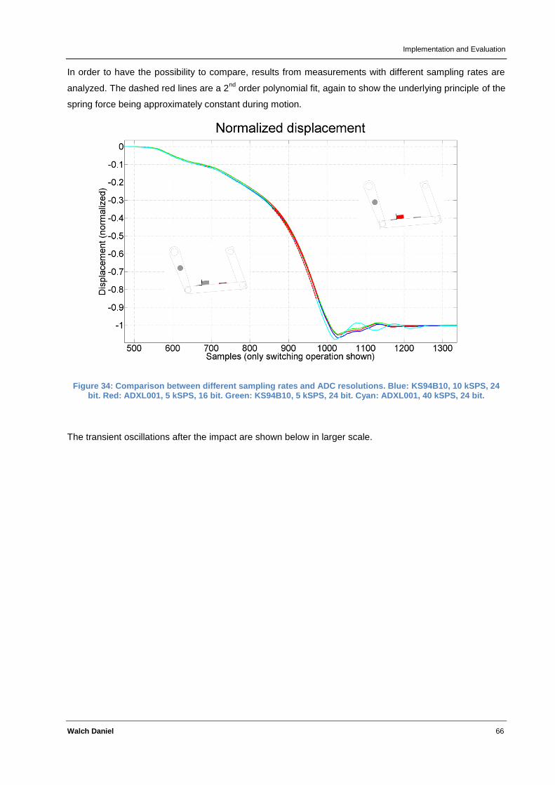
Implementation and Evaluation
Walch Daniel 66
In order to have the possibility to compare, results from measurements with different sampling rates are
analyzed. The dashed red lines are a 2nd
order polynomial fit, again to show the underlying principle of the
spring force being approximately constant during motion.
Figure 34: Comparison between different sampling rates and ADC resolutions. Blue: KS94B10, 10 kSPS, 24 bit. Red: ADXL001, 5 kSPS, 16 bit. Green: KS94B10, 5 kSPS, 24 bit. Cyan: ADXL001, 40 kSPS, 24 bit.
The transient oscillations after the impact are shown below in larger scale.
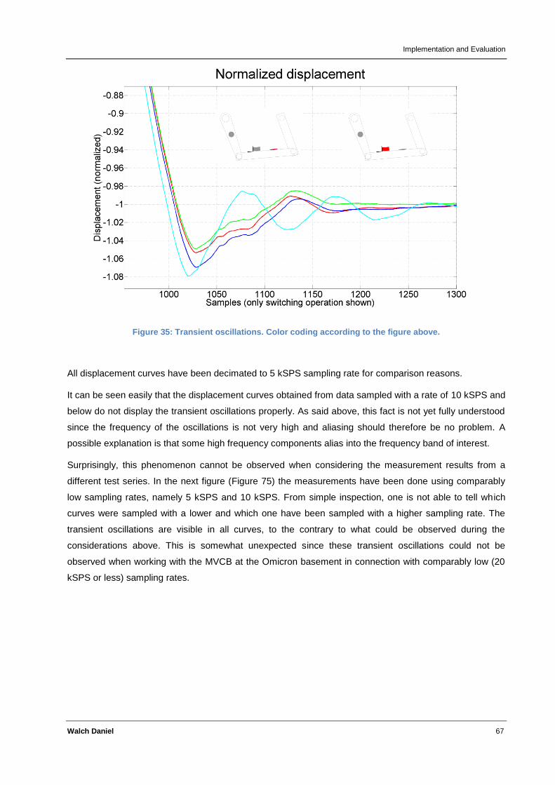
Implementation and Evaluation
Walch Daniel 67
Figure 35: Transient oscillations. Color coding according to the figure above.
All displacement curves have been decimated to 5 kSPS sampling rate for comparison reasons.
It can be seen easily that the displacement curves obtained from data sampled with a rate of 10 kSPS and
below do not display the transient oscillations properly. As said above, this fact is not yet fully understood
since the frequency of the oscillations is not very high and aliasing should therefore be no problem. A
possible explanation is that some high frequency components alias into the frequency band of interest.
Surprisingly, this phenomenon cannot be observed when considering the measurement results from a
different test series. In the next figure (Figure 75) the measurements have been done using comparably
low sampling rates, namely 5 kSPS and 10 kSPS. From simple inspection, one is not able to tell which
curves were sampled with a lower and which one have been sampled with a higher sampling rate. The
transient oscillations are visible in all curves, to the contrary to what could be observed during the
considerations above. This is somewhat unexpected since these transient oscillations could not be
observed when working with the MVCB at the Omicron basement in connection with comparably low (20
kSPS or less) sampling rates.
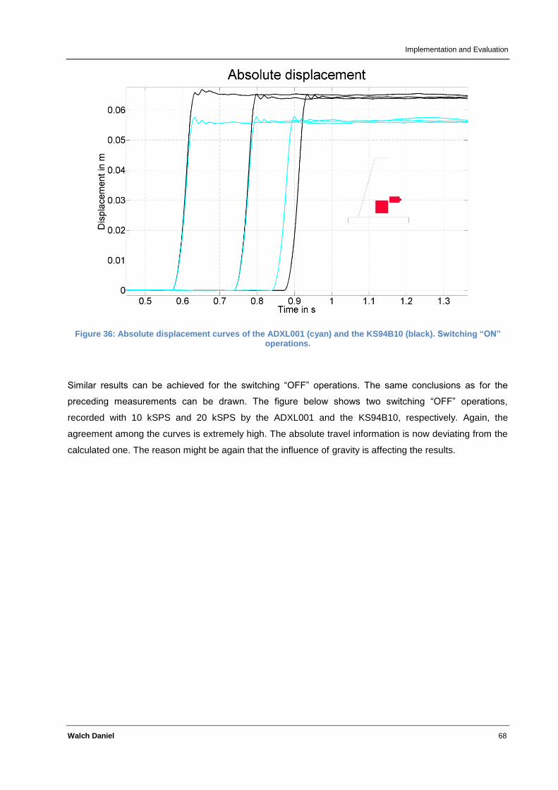
Implementation and Evaluation
Walch Daniel 68
Figure 36: Absolute displacement curves of the ADXL001 (cyan) and the KS94B10 (black). Switching “ON” operations.
Similar results can be achieved for the switching “OFF” operations. The same conclusions as for the
preceding measurements can be drawn. The figure below shows two switching “OFF” operations,
recorded with 10 kSPS and 20 kSPS by the ADXL001 and the KS94B10, respectively. Again, the
agreement among the curves is extremely high. The absolute travel information is now deviating from the
calculated one. The reason might be again that the influence of gravity is affecting the results.
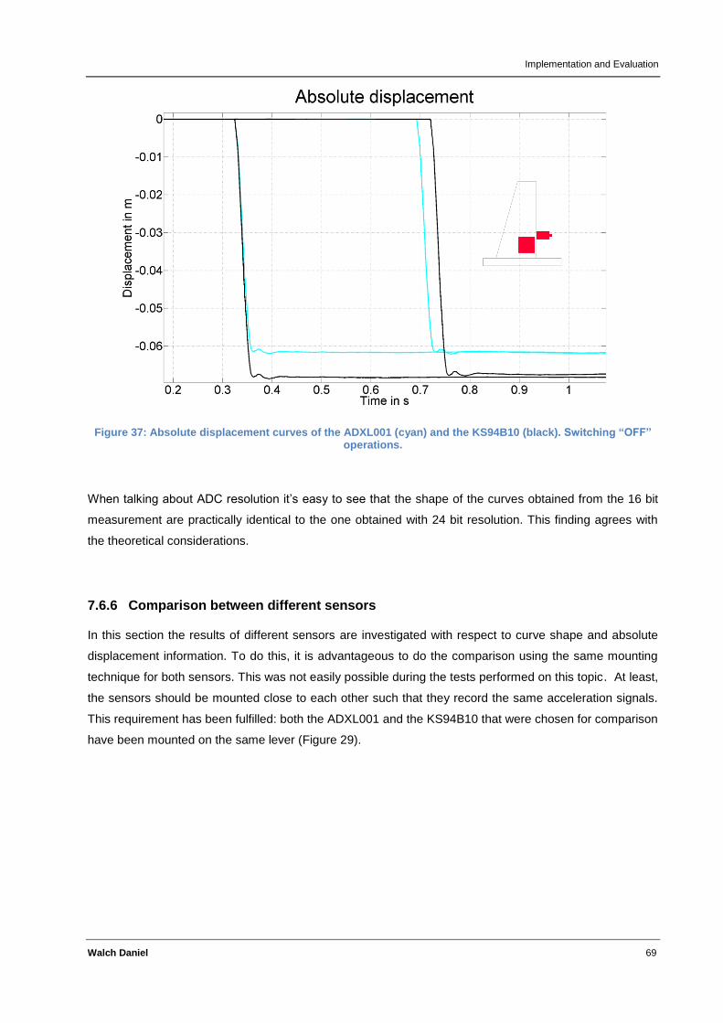
Implementation and Evaluation
Walch Daniel 69
Figure 37: Absolute displacement curves of the ADXL001 (cyan) and the KS94B10 (black). Switching “OFF” operations.
When talking about ADC resolution it’s easy to see that the shape of the curves obtained from the 16 bit
measurement are practically identical to the one obtained with 24 bit resolution. This finding agrees with
the theoretical considerations.
7.6.6 Comparison between different sensors
In this section the results of different sensors are investigated with respect to curve shape and absolute
displacement information. To do this, it is advantageous to do the comparison using the same mounting
technique for both sensors. This was not easily possible during the tests performed on this topic. At least,
the sensors should be mounted close to each other such that they record the same acceleration signals.
This requirement has been fulfilled: both the ADXL001 and the KS94B10 that were chosen for comparison
have been mounted on the same lever (Figure 29).
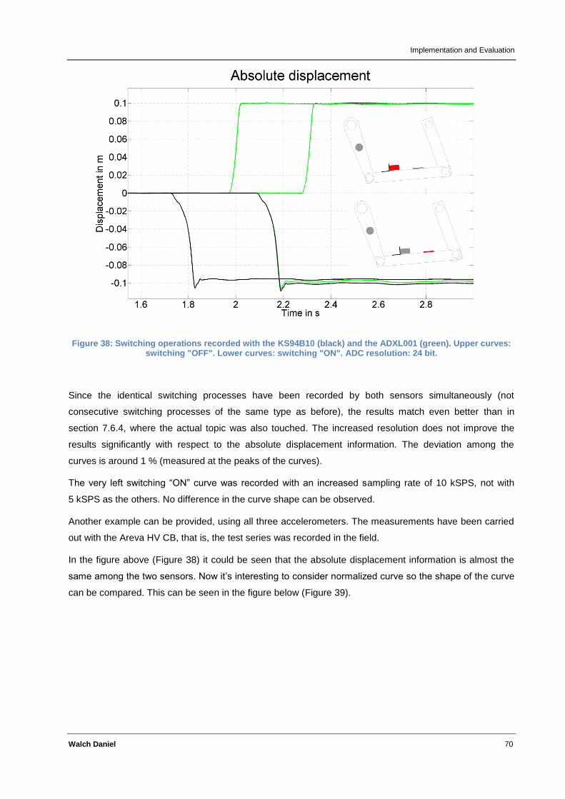
Implementation and Evaluation
Walch Daniel 70
Figure 38: Switching operations recorded with the KS94B10 (black) and the ADXL001 (green). Upper curves: switching "OFF". Lower curves: switching "ON". ADC resolution: 24 bit.
Since the identical switching processes have been recorded by both sensors simultaneously (not
consecutive switching processes of the same type as before), the results match even better than in
section 7.6.4, where the actual topic was also touched. The increased resolution does not improve the
results significantly with respect to the absolute displacement information. The deviation among the
curves is around 1 % (measured at the peaks of the curves).
The very left switching “ON” curve was recorded with an increased sampling rate of 10 kSPS, not with
5 kSPS as the others. No difference in the curve shape can be observed.
Another example can be provided, using all three accelerometers. The measurements have been carried
out with the Areva HV CB, that is, the test series was recorded in the field.
In the figure above (Figure 38) it could be seen that the absolute displacement information is almost the
same among the two sensors. Now it’s interesting to consider normalized curve so the shape of the curve
can be compared. This can be seen in the figure below (Figure 39).
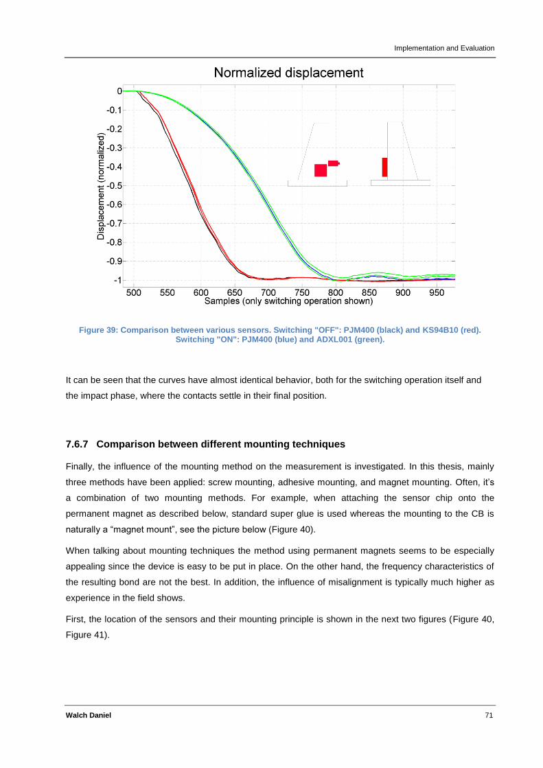
Implementation and Evaluation
Walch Daniel 71
Figure 39: Comparison between various sensors. Switching "OFF": PJM400 (black) and KS94B10 (red). Switching "ON": PJM400 (blue) and ADXL001 (green).
It can be seen that the curves have almost identical behavior, both for the switching operation itself and
the impact phase, where the contacts settle in their final position.
7.6.7 Comparison between different mounting techniques
Finally, the influence of the mounting method on the measurement is investigated. In this thesis, mainly
three methods have been applied: screw mounting, adhesive mounting, and magnet mounting. Often, it’s
a combination of two mounting methods. For example, when attaching the sensor chip onto the
permanent magnet as described below, standard super glue is used whereas the mounting to the CB is
naturally a “magnet mount”, see the picture below (Figure 40).
When talking about mounting techniques the method using permanent magnets seems to be especially
appealing since the device is easy to be put in place. On the other hand, the frequency characteristics of
the resulting bond are not the best. In addition, the influence of misalignment is typically much higher as
experience in the field shows.
First, the location of the sensors and their mounting principle is shown in the next two figures (Figure 40,
Figure 41).
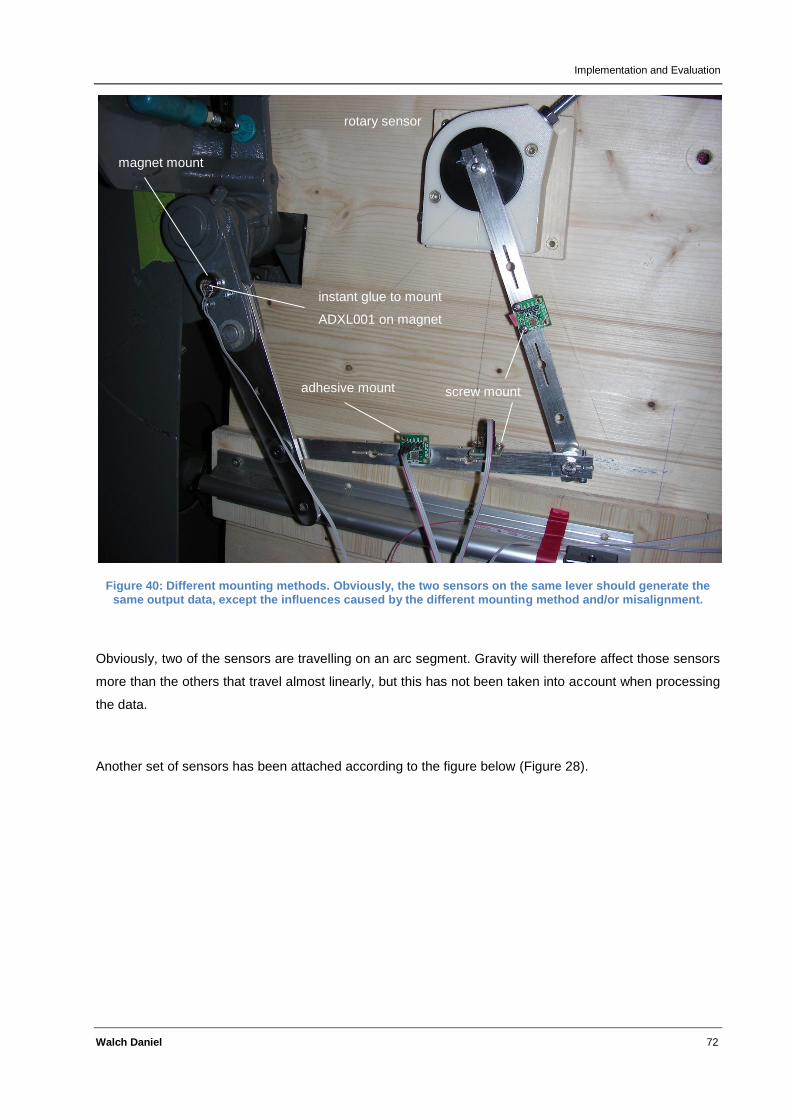
Implementation and Evaluation
Walch Daniel 72
Figure 40: Different mounting methods. Obviously, the two sensors on the same lever should generate the same output data, except the influences caused by the different mounting method and/or misalignment.
Obviously, two of the sensors are travelling on an arc segment. Gravity will therefore affect those sensors
more than the others that travel almost linearly, but this has not been taken into account when processing
the data.
Another set of sensors has been attached according to the figure below (Figure 28).
magnet mount
screw mount
rotary sensor
adhesive mount
instant glue to mount
ADXL001 on magnet
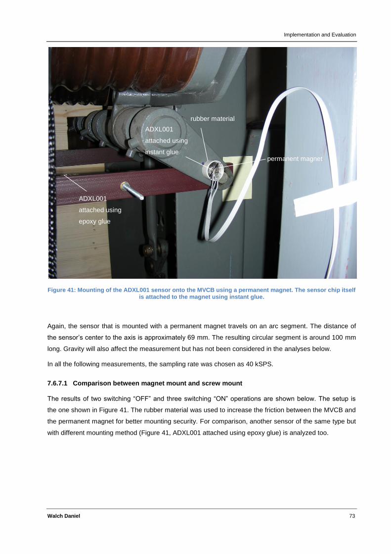
Implementation and Evaluation
Walch Daniel 73
Figure 41: Mounting of the ADXL001 sensor onto the MVCB using a permanent magnet. The sensor chip itself is attached to the magnet using instant glue.
Again, the sensor that is mounted with a permanent magnet travels on an arc segment. The distance of
the sensor’s center to the axis is approximately 69 mm. The resulting circular segment is around 100 mm
long. Gravity will also affect the measurement but has not been considered in the analyses below.
In all the following measurements, the sampling rate was chosen as 40 kSPS.
7.6.7.1 Comparison between magnet mount and screw mount
The results of two switching “OFF” and three switching “ON” operations are shown below. The setup is
the one shown in Figure 41. The rubber material was used to increase the friction between the MVCB and
the permanent magnet for better mounting security. For comparison, another sensor of the same type but
with different mounting method (Figure 41, ADXL001 attached using epoxy glue) is analyzed too.
rubber material
ADXL001
attached using
instant glue permanent magnet
ADXL001
attached using
epoxy glue
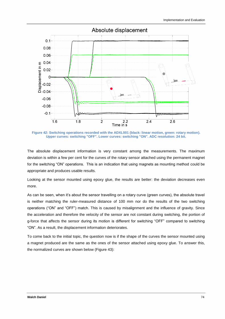
Implementation and Evaluation
Walch Daniel 74
Figure 42: Switching operations recorded with the ADXL001 (black: linear motion, green: rotary motion).
Upper curves: switching "OFF". Lower curves: switching "ON". ADC resolution: 24 bit.
The absolute displacement information is very constant among the measurements. The maximum
deviation is within a few per cent for the curves of the rotary sensor attached using the permanent magnet
for the switching “ON” operations. This is an indication that using magnets as mounting method could be
appropriate and produces usable results.
Looking at the sensor mounted using epoxy glue, the results are better: the deviation decreases even
more.
As can be seen, when it’s about the sensor travelling on a rotary curve (green curves), the absolute travel
is neither matching the ruler-measured distance of 100 mm nor do the results of the two switching
operations (“ON” and “OFF”) match. This is caused by misalignment and the influence of gravity. Since
the acceleration and therefore the velocity of the sensor are not constant during switching, the portion of
g-force that affects the sensor during its motion is different for switching “OFF” compared to switching
“ON”. As a result, the displacement information deteriorates.
To come back to the initial topic, the question now is if the shape of the curves the sensor mounted using
a magnet produced are the same as the ones of the sensor attached using epoxy glue. To answer this,
the normalized curves are shown below (Figure 43):
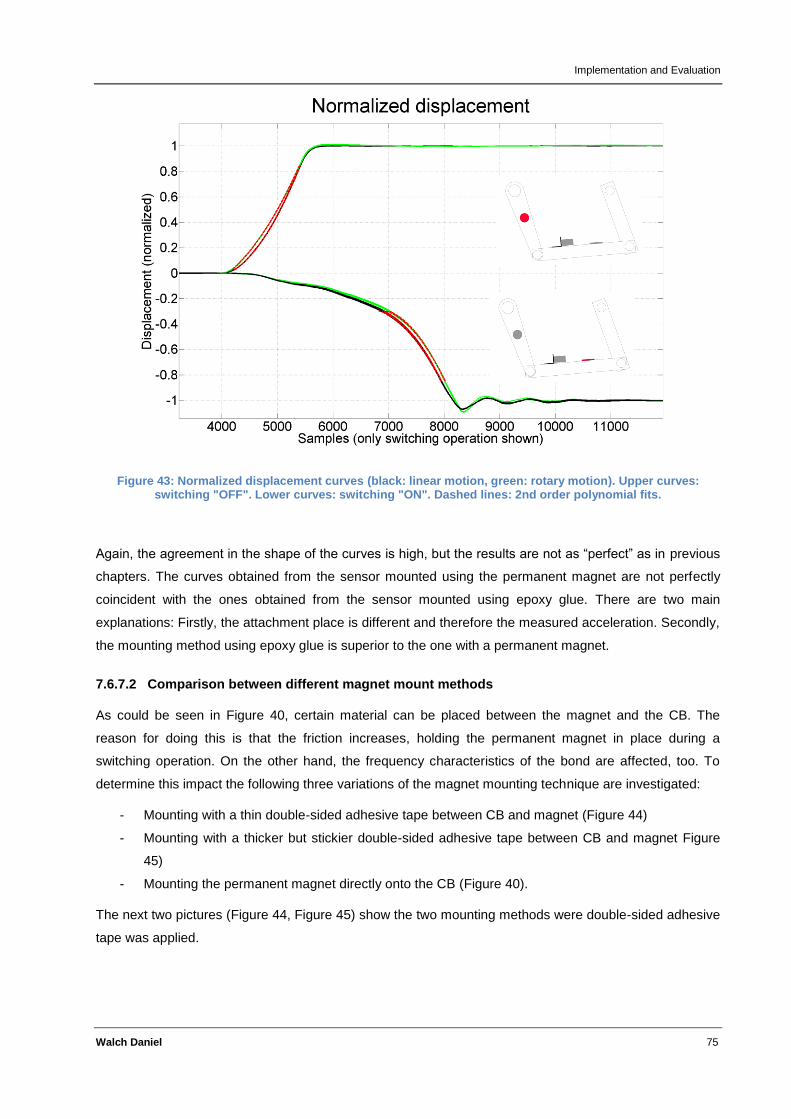
Implementation and Evaluation
Walch Daniel 75
Figure 43: Normalized displacement curves (black: linear motion, green: rotary motion). Upper curves: switching "OFF". Lower curves: switching "ON". Dashed lines: 2nd order polynomial fits.
Again, the agreement in the shape of the curves is high, but the results are not as “perfect” as in previous
chapters. The curves obtained from the sensor mounted using the permanent magnet are not perfectly
coincident with the ones obtained from the sensor mounted using epoxy glue. There are two main
explanations: Firstly, the attachment place is different and therefore the measured acceleration. Secondly,
the mounting method using epoxy glue is superior to the one with a permanent magnet.
7.6.7.2 Comparison between different magnet mount methods
As could be seen in Figure 40, certain material can be placed between the magnet and the CB. The
reason for doing this is that the friction increases, holding the permanent magnet in place during a
switching operation. On the other hand, the frequency characteristics of the bond are affected, too. To
determine this impact the following three variations of the magnet mounting technique are investigated:
- Mounting with a thin double-sided adhesive tape between CB and magnet (Figure 44)
- Mounting with a thicker but stickier double-sided adhesive tape between CB and magnet Figure
45)
- Mounting the permanent magnet directly onto the CB (Figure 40).
The next two pictures (Figure 44, Figure 45) show the two mounting methods were double-sided adhesive
tape was applied.

Implementation and Evaluation
Walch Daniel 76
)
Figure 44: Mounted sensor using a thin double-sided adhesive tape between magnet and MVCB.
Figure 45: Preparing mounting position for the magnet. Thicker double-sided adhesive tape applied between MVCB and the magnet holding the sensor.
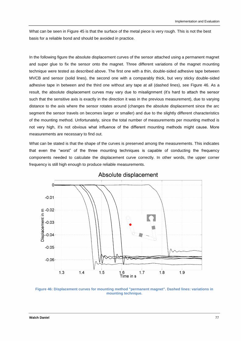
Implementation and Evaluation
Walch Daniel 77
What can be seen in Figure 45 is that the surface of the metal piece is very rough. This is not the best
basis for a reliable bond and should be avoided in practice.
In the following figure the absolute displacement curves of the sensor attached using a permanent magnet
and super glue to fix the sensor onto the magnet. Three different variations of the magnet mounting
technique were tested as described above. The first one with a thin, double-sided adhesive tape between
MVCB and sensor (solid lines), the second one with a comparably thick, but very sticky double-sided
adhesive tape in between and the third one without any tape at all (dashed lines), see Figure 46. As a
result, the absolute displacement curves may vary due to misalignment (it’s hard to attach the sensor
such that the sensitive axis is exactly in the direction it was in the previous measurement), due to varying
distance to the axis where the sensor rotates around (changes the absolute displacement since the arc
segment the sensor travels on becomes larger or smaller) and due to the slightly different characteristics
of the mounting method. Unfortunately, since the total number of measurements per mounting method is
not very high, it’s not obvious what influence of the different mounting methods might cause. More
measurements are necessary to find out.
What can be stated is that the shape of the curves is preserved among the measurements. This indicates
that even the “worst” of the three mounting techniques is capable of conducting the frequency
components needed to calculate the displacement curve correctly. In other words, the upper corner
frequency is still high enough to produce reliable measurements.
Figure 46: Displacement curves for mounting method "permanent magnet". Dashed lines: variations in mounting technique.
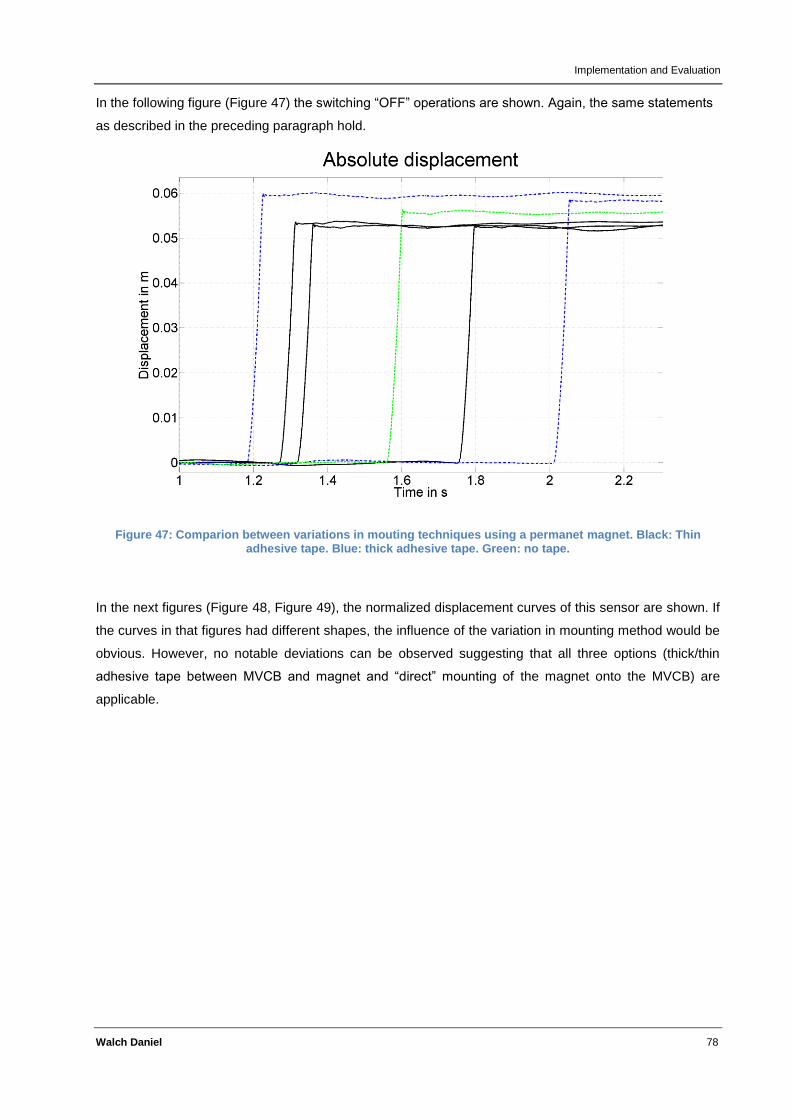
Implementation and Evaluation
Walch Daniel 78
In the following figure (Figure 47) the switching “OFF” operations are shown. Again, the same statements
as described in the preceding paragraph hold.
Figure 47: Comparion between variations in mouting techniques using a permanet magnet. Black: Thin adhesive tape. Blue: thick adhesive tape. Green: no tape.
In the next figures (Figure 48, Figure 49), the normalized displacement curves of this sensor are shown. If
the curves in that figures had different shapes, the influence of the variation in mounting method would be
obvious. However, no notable deviations can be observed suggesting that all three options (thick/thin
adhesive tape between MVCB and magnet and “direct” mounting of the magnet onto the MVCB) are
applicable.
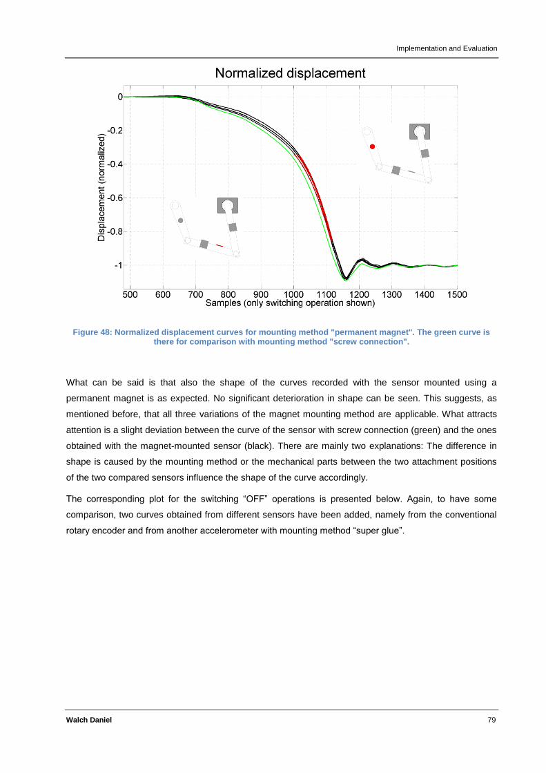
Implementation and Evaluation
Walch Daniel 79
Figure 48: Normalized displacement curves for mounting method "permanent magnet". The green curve is there for comparison with mounting method "screw connection".
What can be said is that also the shape of the curves recorded with the sensor mounted using a
permanent magnet is as expected. No significant deterioration in shape can be seen. This suggests, as
mentioned before, that all three variations of the magnet mounting method are applicable. What attracts
attention is a slight deviation between the curve of the sensor with screw connection (green) and the ones
obtained with the magnet-mounted sensor (black). There are mainly two explanations: The difference in
shape is caused by the mounting method or the mechanical parts between the two attachment positions
of the two compared sensors influence the shape of the curve accordingly.
The corresponding plot for the switching “OFF” operations is presented below. Again, to have some
comparison, two curves obtained from different sensors have been added, namely from the conventional
rotary encoder and from another accelerometer with mounting method “super glue”.
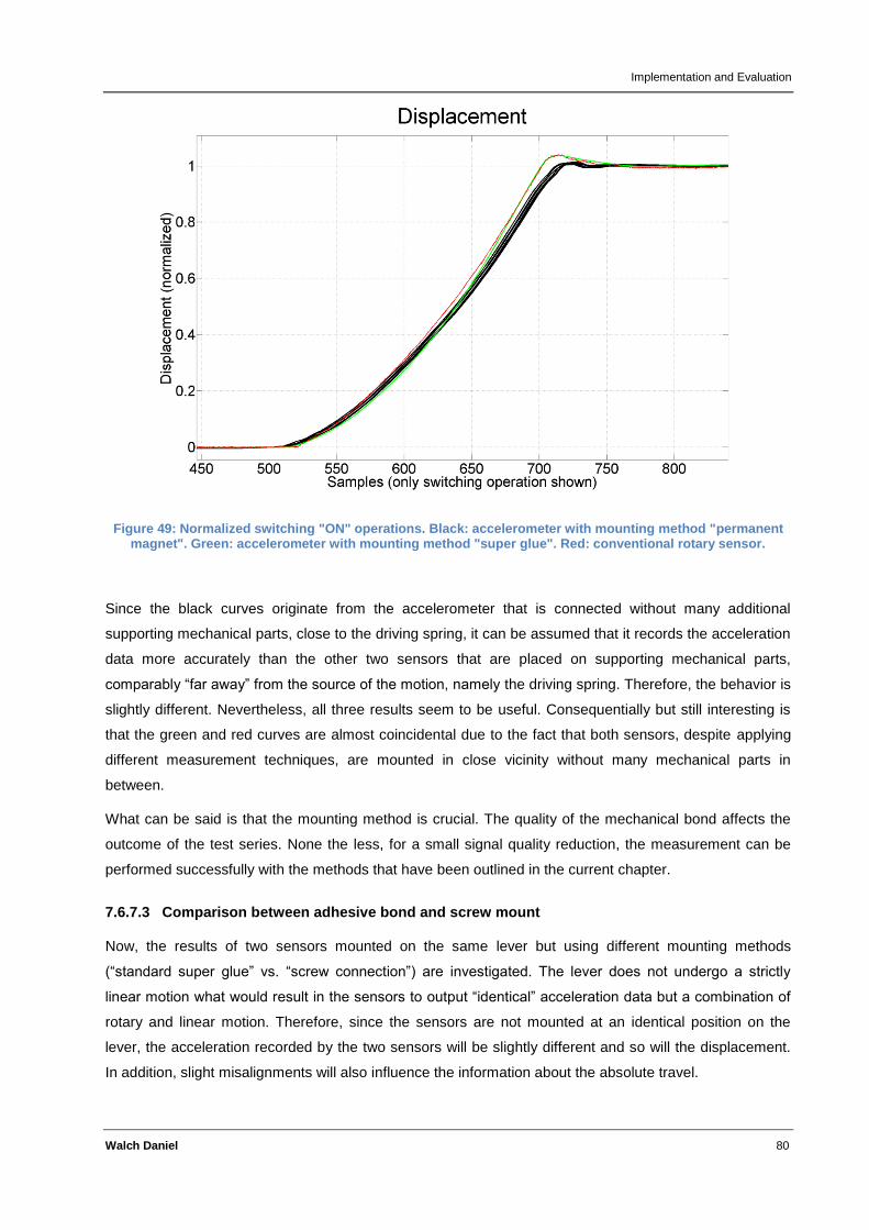
Implementation and Evaluation
Walch Daniel 80
Figure 49: Normalized switching "ON" operations. Black: accelerometer with mounting method "permanent magnet". Green: accelerometer with mounting method "super glue". Red: conventional rotary sensor.
Since the black curves originate from the accelerometer that is connected without many additional
supporting mechanical parts, close to the driving spring, it can be assumed that it records the acceleration
data more accurately than the other two sensors that are placed on supporting mechanical parts,
comparably “far away” from the source of the motion, namely the driving spring. Therefore, the behavior is
slightly different. Nevertheless, all three results seem to be useful. Consequentially but still interesting is
that the green and red curves are almost coincidental due to the fact that both sensors, despite applying
different measurement techniques, are mounted in close vicinity without many mechanical parts in
between.
What can be said is that the mounting method is crucial. The quality of the mechanical bond affects the
outcome of the test series. None the less, for a small signal quality reduction, the measurement can be
performed successfully with the methods that have been outlined in the current chapter.
7.6.7.3 Comparison between adhesive bond and screw mount
Now, the results of two sensors mounted on the same lever but using different mounting methods
(“standard super glue” vs. “screw connection”) are investigated. The lever does not undergo a strictly
linear motion what would result in the sensors to output “identical” acceleration data but a combination of
rotary and linear motion. Therefore, since the sensors are not mounted at an identical position on the
lever, the acceleration recorded by the two sensors will be slightly different and so will the displacement.
In addition, slight misalignments will also influence the information about the absolute travel.
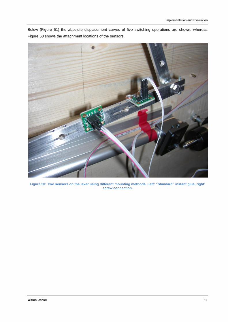
Implementation and Evaluation
Walch Daniel 81
Below (Figure 51) the absolute displacement curves of five switching operations are shown, whereas
Figure 50 shows the attachment locations of the sensors.
Figure 50: Two sensors on the lever using different mounting methods. Left: “Standard” instant glue, right: screw connection.
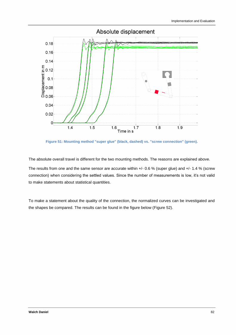
Implementation and Evaluation
Walch Daniel 82
Figure 51: Mounting method "super glue" (black, dashed) vs. "screw connection" (green).
The absolute overall travel is different for the two mounting methods. The reasons are explained above.
The results from one and the same sensor are accurate within +/- 0.6 % (super glue) and +/- 1.4 % (screw
connection) when considering the settled values. Since the number of measurements is low, it’s not valid
to make statements about statistical quantities.
To make a statement about the quality of the connection, the normalized curves can be investigated and
the shapes be compared. The results can be found in the figure below (Figure 52).
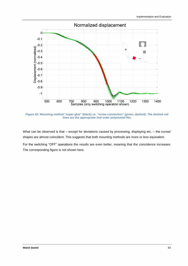
Implementation and Evaluation
Walch Daniel 83
Figure 52: Mounting method "super glue" (black) vs. "screw connection" (green, dashed). The dashed red lines are the appropriate 2nd order polynomial fits.
What can be observed is that – except for deviations caused by processing, displaying etc. – the curves’
shapes are almost coincident. This suggests that both mounting methods are more or less equivalent.
For the switching “OFF” operations the results are even better, meaning that the coincidence increases.
The corresponding figure is not shown here.
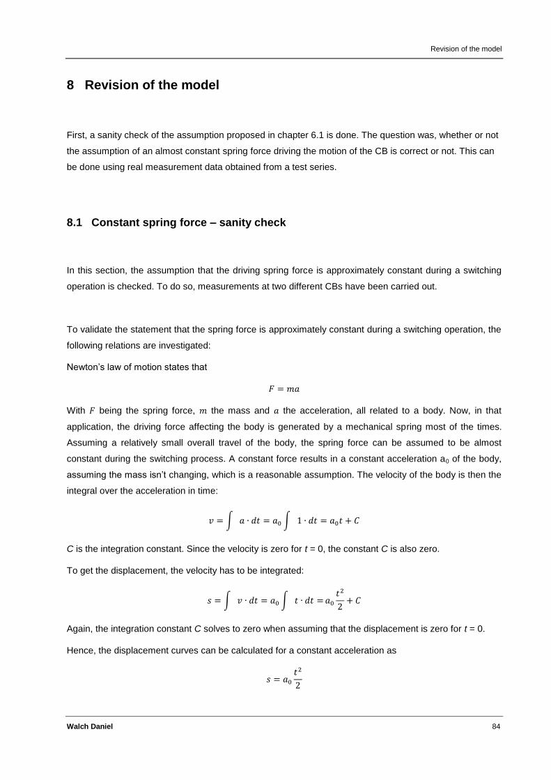
Revision of the model
Walch Daniel 84
8 Revision of the model
First, a sanity check of the assumption proposed in chapter 6.1 is done. The question was, whether or not
the assumption of an almost constant spring force driving the motion of the CB is correct or not. This can
be done using real measurement data obtained from a test series.
8.1 Constant spring force – sanity check
In this section, the assumption that the driving spring force is approximately constant during a switching
operation is checked. To do so, measurements at two different CBs have been carried out.
To validate the statement that the spring force is approximately constant during a switching operation, the
following relations are investigated:
Newton’s law of motion states that
With being the spring force, the mass and the acceleration, all related to a body. Now, in that
application, the driving force affecting the body is generated by a mechanical spring most of the times.
Assuming a relatively small overall travel of the body, the spring force can be assumed to be almost
constant during the switching process. A constant force results in a constant acceleration a0 of the body,
assuming the mass isn’t changing, which is a reasonable assumption. The velocity of the body is then the
integral over the acceleration in time:
∫ ∫
C is the integration constant. Since the velocity is zero for t = 0, the constant C is also zero.
To get the displacement, the velocity has to be integrated:
∫ ∫
Again, the integration constant C solves to zero when assuming that the displacement is zero for t = 0.
Hence, the displacement curves can be calculated for a constant acceleration as
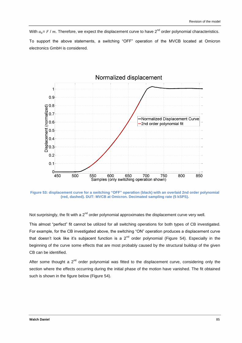
Revision of the model
Walch Daniel 85
With = / . Therefore, we expect the displacement curve to have 2nd
order polynomial characteristics.
To support the above statements, a switching “OFF” operation of the MVCB located at Omicron
electronics GmbH is considered.
Figure 53: displacement curve for a switching “OFF” operation (black) with an overlaid 2nd order polynomial (red, dashed). DUT: MVCB at Omicron. Decimated sampling rate (5 kSPS).
Not surprisingly, the fit with a 2nd
order polynomial approximates the displacement curve very well.
This almost “perfect” fit cannot be utilized for all switching operations for both types of CB investigated.
For example, for the CB investigated above, the switching “ON” operation produces a displacement curve
that doesn’t look like it’s subjacent function is a 2nd
order polynomial (Figure 54). Especially in the
beginning of the curve some effects that are most probably caused by the structural buildup of the given
CB can be identified.
After some thought a 2nd
order polynomial was fitted to the displacement curve, considering only the
section where the effects occurring during the initial phase of the motion have vanished. The fit obtained
such is shown in the figure below (Figure 54).
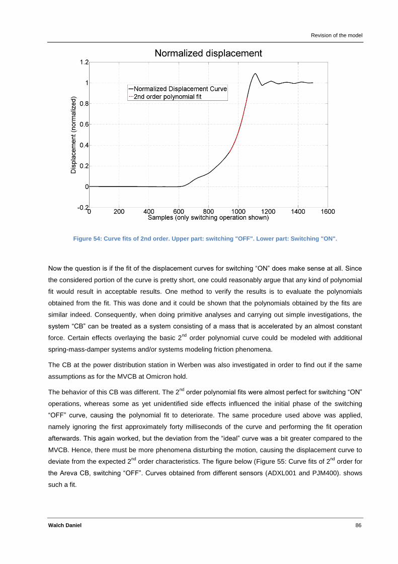
Revision of the model
Walch Daniel 86
Figure 54: Curve fits of 2nd order. Upper part: switching "OFF". Lower part: Switching "ON".
Now the question is if the fit of the displacement curves for switching “ON” does make sense at all. Since
the considered portion of the curve is pretty short, one could reasonably argue that any kind of polynomial
fit would result in acceptable results. One method to verify the results is to evaluate the polynomials
obtained from the fit. This was done and it could be shown that the polynomials obtained by the fits are
similar indeed. Consequently, when doing primitive analyses and carrying out simple investigations, the
system “CB” can be treated as a system consisting of a mass that is accelerated by an almost constant
force. Certain effects overlaying the basic 2nd
order polynomial curve could be modeled with additional
spring-mass-damper systems and/or systems modeling friction phenomena.
The CB at the power distribution station in Werben was also investigated in order to find out if the same
assumptions as for the MVCB at Omicron hold.
The behavior of this CB was different. The 2nd
order polynomial fits were almost perfect for switching “ON”
operations, whereas some as yet unidentified side effects influenced the initial phase of the switching
“OFF” curve, causing the polynomial fit to deteriorate. The same procedure used above was applied,
namely ignoring the first approximately forty milliseconds of the curve and performing the fit operation
afterwards. This again worked, but the deviation from the “ideal” curve was a bit greater compared to the
MVCB. Hence, there must be more phenomena disturbing the motion, causing the displacement curve to
deviate from the expected 2nd
order characteristics. The figure below (Figure 55: Curve fits of 2nd
order for
the Areva CB, switching “OFF”. Curves obtained from different sensors (ADXL001 and PJM400). shows
such a fit.
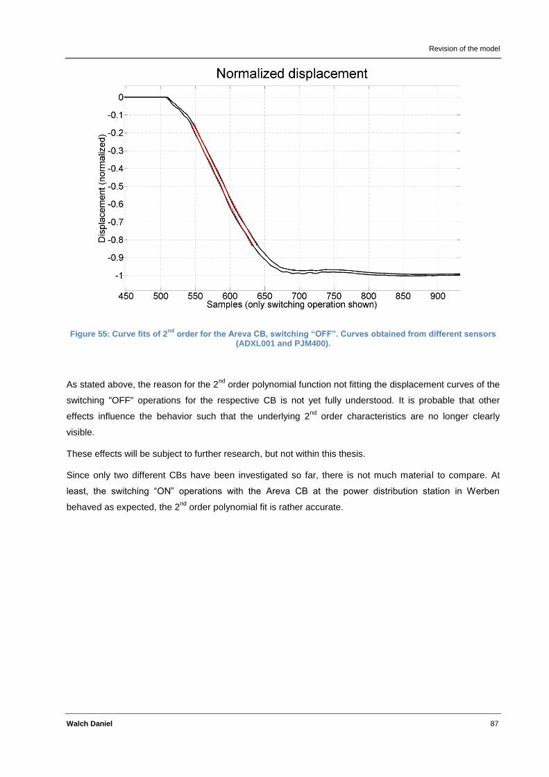
Revision of the model
Walch Daniel 87
Figure 55: Curve fits of 2nd
order for the Areva CB, switching “OFF”. Curves obtained from different sensors (ADXL001 and PJM400).
As stated above, the reason for the 2nd
order polynomial function not fitting the displacement curves of the
switching "OFF" operations for the respective CB is not yet fully understood. It is probable that other
effects influence the behavior such that the underlying 2nd
order characteristics are no longer clearly
visible.
These effects will be subject to further research, but not within this thesis.
Since only two different CBs have been investigated so far, there is not much material to compare. At
least, the switching “ON” operations with the Areva CB at the power distribution station in Werben
behaved as expected, the 2nd
order polynomial fit is rather accurate.
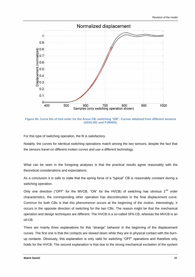
Revision of the model
Walch Daniel 88
Figure 56: Curve fits of 2nd order for the Areva CB, switching “ON”. Curves obtained from different sensors (ADXL001 and PJM400).
For this type of switching operation, the fit is satisfactory.
Notably, the curves for identical switching operations match among the two sensors, despite the fact that
the sensors travel on different motion curves and use a different technology.
What can be seen in the foregoing analyses is that the practical results agree reasonably with the
theoretical considerations and expectations.
As a conclusion it is safe to state that the spring force of a “typical” CB is reasonably constant during a
switching operation.
Only one direction (“OFF” for the MVCB, “ON” for the HVCB) of switching has obvious 2nd
order
characteristics, the corresponding other operation has discontinuities in the final displacement curve.
Common for both CBs is that this phenomenon occurs at the beginning of the motion. Interestingly, it
occurs in the opposite direction of switching for the two CBs. The reason might be that the mechanical
operation and design techniques are different. The HVCB is a so-called SF6-CB, whereas the MVCB is an
oil-CB.
There are mainly three explanations for this “strange” behavior in the beginning of the displacement
curves. The first one is that the contacts are slowed down while they are in physical contact with the burn-
up contacts. Obviously, this explanation is only valid for switching “OFF” operations and therefore only
holds for the HVCB. The second explanation is that due to the strong mechanical excitation of the system
Revision of the model
Walch Daniel 89
when starting a switching operation (“releasing the spring force”) various transient, decaying oscillations
occur. This might be true for the MVCB. What is contradictory to this statement is that no constant period
for the oscillations could be found. In addition, it was not possible to superimpose a 2nd
order polynomial
with a damped trigonometric function (sine, cosine) and fit the resulting displacement curve. If only these
oscillations occurred, one could justifiable argue that by a superposition of a 2nd
order polynomial, a
decaying exponential function and a trigonometric function it should be possible to approximate the
displacement curve. In conclusion, it’s expected that if oscillations really occur physically at the
accelerometer, there must be other phenomena overlying these. The third explanation is that there are
strong magnetic fields interacting with the measurement equipment. This explanation would have to be
investigated thoroughly to give it a reliable basis.
When looking at the curve in Figure 56: Curve fits of 2nd order for the Areva CB, switching “ON”. Curves
obtained from different sensors (ADXL001 and PJM400)., the first part of the curve has been excluded
from the curve fitting procedure. The shape of the curve is hard to be interpreted. The first part may – as
stated above – be influenced by an additional friction against the direction of the motion, caused for
example by physical friction of the main contacts with the burn-up contacts. In the data series available, it
looks like this first part of the figure is approximately linear with some oscillations/disturbances on it. The
2nd
piece of the curve that would be assumed to have 2nd order polynomial characteristics is also hard to
analyze. From the figure, it can be stated that a 2nd
order fit is a bit better than a 1st or 3
rd order fit, but
doesn’t make too much of a difference. Hence, stating that this part of the curve follows a polynomial of
degree two lacks a reliable basis.
8.1.1 Conclusion
In this chapter it could be shown that it seems that the assumption that the driving force of the mechanical
spring in a circuit breaker can be assumed to be almost constant during a switching operation. Hence, the
basic underlying characteristics of the displacement curve of the contacts in a CB can be described using
the simple model introduced in section 6.1.
The fact that the displacement curve as a whole obtained from the measurements cannot be modeled
satisfactory with the simple model introduced in section 6.1 raise the need for a better, more sophisticated
model. As mentioned several times, not much knowledge about the mechanical structure of the CBs is
available what makes it tedious and somewhat a “guessing game” to invent an appropriate model “from
scratch”. Instead, after having calculated some displacement curves, the reverse approach is made:
taking the displacement curve as a reference, it’s tried to find a suitable model that would “generate” such
a displacement curve. Naturally, this technique requires measurement data and its evaluation to be
present; therefore this approach is presented later in this thesis in section 8.2.

Revision of the model
Walch Daniel 90
8.2 Detailed model
Now that we have a large number of displacement curves available, the attempt of inventing a more
complex model to describe the character of such a displacement curve can be made.
To develop this model, a different approach compared to the simple model in section 6.1 was used. The
final displacement curve is taken as a reference and “rebuilt” by an interpolating function. This function
has several parameters that determine the shape of the resulting curve. Hence, the parameter set of this
function is a model for the displacement curve. To obtain a set of parameters that models the
displacement curve best, optimization can be done. Basically, the only data that is available to make a
statement about the quality of the approximation is the pure acceleration signal. Thus, the modeled
displacement signal has to be differentiated twice to obtain the “simulated” acceleration signal. This
simulated signal can be compared to the measured one and a certain objective function can be used to
rate the quality of the approximation.
The following constraints have to be fulfilled by the interpolating function:
- twice differentiable, since the displacement signal has to be differentiated twice to get the
acceleration signal
- continuous displacement signal (no “jumps” in the displacement signal)
- continuous velocity signal (no “jumps” in the velocity signal)
- initial position, velocity and acceleration are zero
- final velocity and acceleration are zero
- “smoothness”: the displacement curve has hardly any high frequency oscillating behavior (not
implemented explicitly yet)
One could also state that the acceleration signal has also to be continuous. This is perfectly true in the
real world. Since the acceleration signal, as is known from various measurements, is not showing any
kind of “smooth” behavior rather than changing rapidly in amplitude the argument is that even between to
sampling points the acceleration changes significantly. Therefore, this statement is somewhat woolly.
Nevertheless, an interpolating function was chosen that even fulfills the statement above: cubic spline
interpolation. Cubic splines have per definition C2-characteristics (twice continuously differentiable) and
avoid the often unwanted effect of oscillation that often occurs when using “standard” polynomial
interpolation [66]. Further information about the basics of spline interpolation can be found in various
sources dealing with numerical mathematics [67], [68], [69], [70].
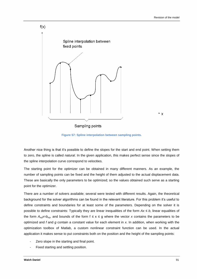
Revision of the model
Walch Daniel 91
Figure 57: Spline interpolation between sampling points.
Another nice thing is that it’s possible to define the slopes for the start and end point. When setting them
to zero, the spline is called natural. In the given application, this makes perfect sense since the slopes of
the spline interpolation curve correspond to velocities.
The starting point for the optimizer can be obtained in many different manners. As an example, the
number of sampling points can be fixed and the height of them adjusted to the actual displacement data.
These are basically the only parameters to be optimized; so the values obtained such serve as a starting
point for the optimizer.
There are a number of solvers available; several were tested with different results. Again, the theoretical
background for the solver algorithms can be found in the relevant literature. For this problem it’s useful to
define constraints and boundaries for at least some of the parameters. Depending on the solver it is
possible to define constraints: Typically they are linear inequalities of the form Ax ≤ b, linear equalities of
the form Aeqx=beq, and bounds of the form f ≤ x ≤ g where the vector x contains the parameters to be
optimized and f and g contain a constant value for each element in x. In addition, when working with the
optimization toolbox of Matlab, a custom nonlinear constraint function can be used. In the actual
application it makes sense to put constraints both on the position and the height of the sampling points:
- Zero slope in the starting and final point.
- Fixed starting and settling position.

Revision of the model
Walch Daniel 92
- Consecutive sampling points may not overlap.
- The height of the sampling points must stay within meaningful borders.
- The constant offset can also be bound.
The vector x consists of 2n+1 elements with n the number of sampling points: n elements containing the
position, n elements containing the height of the sampling points and one element representing the offset.
[
]
More precisely, the following requirements must be met:
with xi being the position of the sampling points and n the number of sampling points.
Rearranging the inequalities leads to
Finally, this can be written in the form Ax ≤ b using the following matrices and vectors:
n n + 1
[
]
[
]
[ ]
To guarantee a “strictly smaller” relation, a small constant term can be considered in the elements of b.
There are no specific restrictions on the height of the sampling points. They can simply be bound within
meaningful limits resulting from the maximum displacement that can be expected for a certain switching
operation.
Revision of the model
Walch Daniel 93
To practically “fix” the starting and settling point, the corresponding upper and lower bounds can be
assigned identical values. This holds for both the position (it’s not desired for the initial and final sampling
point to change their position in time) and the height (starting displacement is typically zero and the
settling position can be fixed as well) of these sampling points
The optimizer is fed with a scalar objective function that it tries to optimize. A simple and often used
function is a mean square error (MSE) algorithm. It compares the desired signal with the simulated one
and squares the error to avoid possible cancellations of the errors due to different signs. The MSE is
determined as
√
∑( )
with asim being the simulated (calculated from the spline fit) and ameas being the measured acceleration
signal and N the number of data points. To get more convenient numbers, the value can as well be
expressed in dB.
When running the optimizer it turned out that it’s both very time and resource consuming to evaluate the
objective function. No intense investigations have been carried out on the task of optimizing the
implementation of the MSE as a Matlab m-file. The number of variables to be optimized is 2n with n the
number of sampling points for the spline fit. This value can also become high, increasing the work load for
the optimizer.
Exhaustive optimization has not been carried out so far, instead the optimizing process was interrupted
after some time. Therefore, the parameter set that serves as a model could further be improved both by
increasing the number of iterations. Another option was to choose the sampling points more carefully and
feed the optimizer with a better “initial guess” of the parameter set.
In addition, other optimization techniques than the ones used might be worth testing for this optimization
problem. To conclude, some effort could be put into this topic to further improve the results. Anyway,
without claiming to have found the “perfect” solution, an optimization process would look like the following:
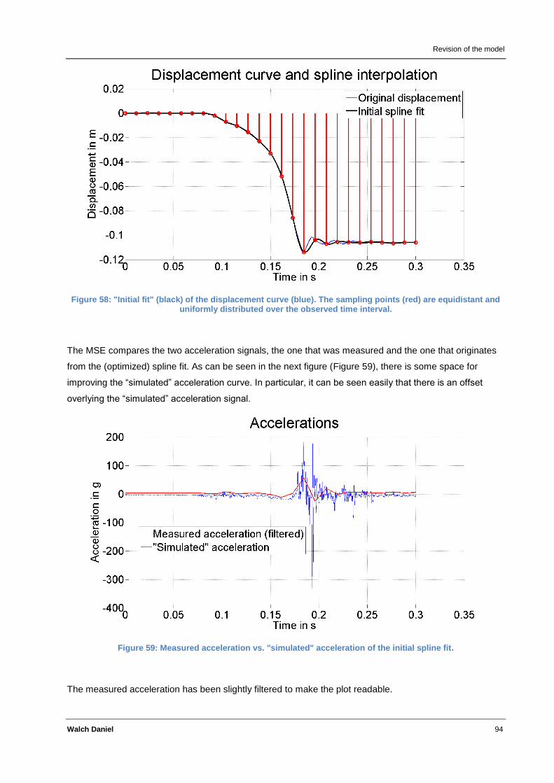
Revision of the model
Walch Daniel 94
Figure 58: "Initial fit" (black) of the displacement curve (blue). The sampling points (red) are equidistant and uniformly distributed over the observed time interval.
The MSE compares the two acceleration signals, the one that was measured and the one that originates
from the (optimized) spline fit. As can be seen in the next figure (Figure 59), there is some space for
improving the “simulated” acceleration curve. In particular, it can be seen easily that there is an offset
overlying the “simulated” acceleration signal.
Figure 59: Measured acceleration vs. "simulated" acceleration of the initial spline fit.
The measured acceleration has been slightly filtered to make the plot readable.
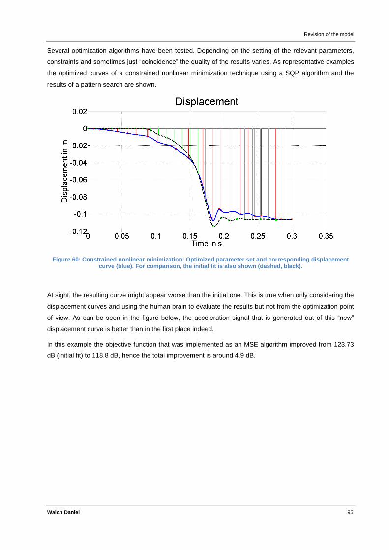
Revision of the model
Walch Daniel 95
Several optimization algorithms have been tested. Depending on the setting of the relevant parameters,
constraints and sometimes just “coincidence” the quality of the results varies. As representative examples
the optimized curves of a constrained nonlinear minimization technique using a SQP algorithm and the
results of a pattern search are shown.
Figure 60: Constrained nonlinear minimization: Optimized parameter set and corresponding displacement curve (blue). For comparison, the initial fit is also shown (dashed, black).
At sight, the resulting curve might appear worse than the initial one. This is true when only considering the
displacement curves and using the human brain to evaluate the results but not from the optimization point
of view. As can be seen in the figure below, the acceleration signal that is generated out of this “new”
displacement curve is better than in the first place indeed.
In this example the objective function that was implemented as an MSE algorithm improved from 123.73
dB (initial fit) to 118.8 dB, hence the total improvement is around 4.9 dB.
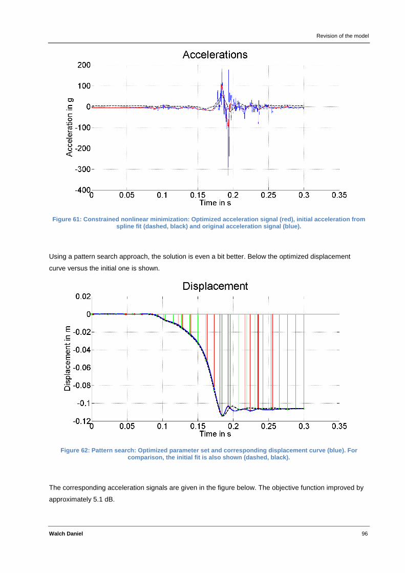
Revision of the model
Walch Daniel 96
Figure 61: Constrained nonlinear minimization: Optimized acceleration signal (red), initial acceleration from spline fit (dashed, black) and original acceleration signal (blue).
Using a pattern search approach, the solution is even a bit better. Below the optimized displacement
curve versus the initial one is shown.
Figure 62: Pattern search: Optimized parameter set and corresponding displacement curve (blue). For comparison, the initial fit is also shown (dashed, black).
The corresponding acceleration signals are given in the figure below. The objective function improved by
approximately 5.1 dB.
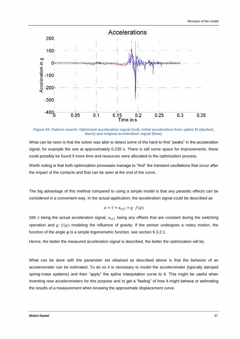
Revision of the model
Walch Daniel 97
Figure 63: Pattern search: Optimized acceleration signal (red), initial acceleration from spline fit (dashed, black) and original acceleration signal (blue).
What can be seen is that the solver was able to detect some of the hard-to-find “peaks” in the acceleration
signal, for example the one at approximately 0.235 s. There is still some space for improvements, these
could possibly be found if more time and resources were allocated to the optimization process.
Worth noting is that both optimization processes manage to “find” the transient oscillations that occur after
the impact of the contacts and that can be seen at the end of the curve.
The big advantage of this method compared to using a simple model is that any parasitic effects can be
considered in a convenient way. In the actual application, the acceleration signal could be described as
( )
Sith being the actual acceleration signal, being any offsets that are constant during the switching
operation and ( ) modeling the influence of gravity. If the sensor undergoes a rotary motion, the
function of the angle φ is a simple trigonometric function, see section 6.3.2.1.
Hence, the better the measured acceleration signal is described, the better the optimization will be.
What can be done with the parameter set obtained as described above is that the behavior of an
accelerometer can be estimated. To do so it is necessary to model the accelerometer (typically damped
spring-mass systems) and then “apply” the spline interpolation curve to it. This might be useful when
inventing new accelerometers for this purpose and to get a “feeling” of how it might behave or estimating
the results of a measurement when knowing the approximate displacement curve.
Discussion
Walch Daniel 98
9 Discussion
In this section, the results obtained throughout this work are discussed. It is evaluated if the requirements
have been met and to what extent the approach presented in this thesis could satisfy the task. Topics that
are still subject to investigation or ones that require further evaluation are listed and suggestions how to
deal with them are given. Further on, conclusions are drawn and future prospects are presented.
9.1 Basic Concluding
After carrying out theoretical and practical considerations, the following statements can be made
concerning the fulfillment of the requirements:
- Measuring the displacement of the switching contacts within circuit breakers using
accelerometers is feasible and at least the relative displacement can be determined.
- The method of choice is competitive to conventional approaches in terms of both cost and
convenience.
- Under certain (normal) circumstances the accuracy of the innovative method is at least
comparable if not superior to the one achieved with conventional methods.
- There are some indications that suggest that the displacement curve is qualitatively correct. The
main indication is that the shape of the curve obtained from the accelerometer measurements
match the ones obtained with conventional linear or rotary encoders.
- Reproducibility can be guaranteed in terms of relative displacement information and shape of the
curve, respectively, even if a mounting mismatch occurs. This holds if the mounting method and
the location of attachment is (approximately) the same.
- Several mounting methods are possible to successfully carry out measurements. Generally
speaking, the attachment of the measuring equipment is far more convenient as for other
techniques used so far and the influence of the measuring equipment on the device under test is
less if even existing to a measurable extent.
- A more careful and sophisticated evaluation of the raw data is necessary compared to the effort
needed to evaluate the conventional method but on the other hand, the influence of certain
parasitic influences can be reduced or eliminated. The quality of the results enhances with the
quality of the mounting method, increasing sampling rate, proper data processing, and considered
choice of attachment location.
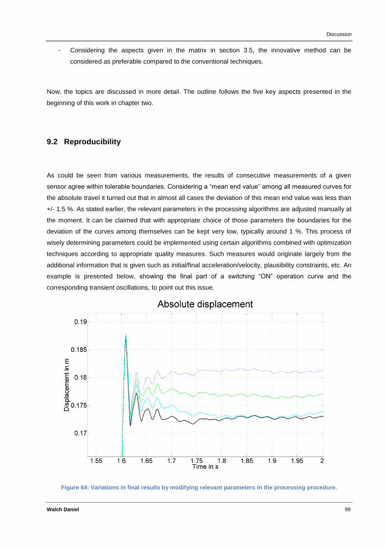
Discussion
Walch Daniel 99
- Considering the aspects given in the matrix in section 3.5, the innovative method can be
considered as preferable compared to the conventional techniques.
Now, the topics are discussed in more detail. The outline follows the five key aspects presented in the
beginning of this work in chapter two.
9.2 Reproducibility
As could be seen from various measurements, the results of consecutive measurements of a given
sensor agree within tolerable boundaries. Considering a “mean end value” among all measured curves for
the absolute travel it turned out that in almost all cases the deviation of this mean end value was less than
+/- 1.5 %. As stated earlier, the relevant parameters in the processing algorithms are adjusted manually at
the moment. It can be claimed that with appropriate choice of those parameters the boundaries for the
deviation of the curves among themselves can be kept very low, typically around 1 %. This process of
wisely determining parameters could be implemented using certain algorithms combined with optimization
techniques according to appropriate quality measures. Such measures would originate largely from the
additional information that is given such as initial/final acceleration/velocity, plausibility constraints, etc. An
example is presented below, showing the final part of a switching “ON” operation curve and the
corresponding transient oscillations, to point out this issue.
Figure 64: Variations in final results by modifying relevant parameters in the processing procedure.
Discussion
Walch Daniel 100
Obviously, varying relevant parameters affects the final displacement curve while the shape
characteristics (frequency of the transient oscillations) itself remain more or less unchanged.
Concerning reproducibility, the results from the accelerometer measurements and from the conventional
encoder are both useful and of approximately the same quality. For better analysis of the reproducibility of
consecutive measurements with the rotary encoder it would be necessary to calibrate the sensor prior to
each measurement.
It has to be said that the measurement data gathered during the studies are probably not a sufficiently
large sample space to make reliable statements about the reproducibility statistics of both techniques. To
support the conclusion made above, more measurement series, possibly considering several types of
sensors would be necessary.
9.3 Accuracy
In this thesis, the term “accuracy” refers to as the precision of the absolute travel information determined
using the acceleration data produced by the sensor. Since both pure rotary as well as combinations of
rotary and linear motions are not processed perfectly at this stage, it’s only valid to consider (almost)
linear translations.
Since only two sensors meet this restriction, the results of these accelerometers have to be considered.
They are mounted on the same lever and undergo a motion of approximately 10 cm. The motion is almost
linear; hence the influence of gravity on the measurement is not too big. Further description of the
attachment of the sensors is given in 7.6.1.1.
As the results show, the accuracy that can be achieved is high. Typically, with proper processing settings,
the deviation from the expected value of 0.1 m can be kept below 1 %.
For the case where the sensor travels on a more complex curve, processing algorithms will have to be
improved to achieve results with the same accuracy. Even better, if a two-dimensional sensor would be
used, combining the outputs in both directions, any motion that occurs in a plane could be evaluated
correctly and with good accuracy.
The main aspects that influence the accuracy at this stage of work are:
- processing algorithms, proper choice of parameters
- “linearity” of the motion curve
- AD-conversion influences at least the settled value of the displacement curve
- g-force for nonlinear motions
Therefore, the main challenges in improving the existing solution are processing and correction of the
influence of gravity (see chapter 6.3.2.).

Discussion
Walch Daniel 101
A conventional sensor would also be capable of measuring the absolute displacement if it’s mounted
properly and the motion is strictly linear. The accuracy is expected to be within the same dimensions as
for the accelerometers. On the contrary, absolute measurement of rotary or combined linear and rotary
motions cannot be performed without further information. If such a measurement is desired, two of these
sensors would have to be mounted exactly perpendicular to each other and the combined displacement
curve be determined by considering both sensor output signals.
This fact is a drawback of the conventional method.
9.4 Quality
The term “quality” in this context means, how well the shape of the displacement curves maintains during
several measurements.
This criterion can be observed best when looking at the “normalized displacement” curves. As can be
seen from various measurements, the quality of the coincidence of the curves from consecutive
measurements is largely determined by the processing procedure. Proper positioning and normalizing of
the curves to be overlaid is essential. If this is carried out carefully, the curves are practically
indistinguishable. A constraint has to be met: the sampling rate must be the same. Sampling with lower
frequencies results in differing curve shapes especially for the transient oscillations that occur especially
in the switching “ON” operations.
It can be assumed that the sampling rate doesn’t play such an important role when working with
conventional encoders since aliasing will not be an issue. Similar to the results of the accelerometer
technique, the quality of the measurements is high and the curves are almost coincident.
Again, the foregoing statements only hold if proper processing is performed.
9.5 Attachment
The attachment is probably one of the most convincing reasons to favor the accelerometer technique over
the conventional measurement methods.
Whereas the comparably large conventional sensors require additional, bulky material to guarantee an
appropriate connection to the device under test, the small and light-weight accelerometers can be
attached more easily. In addition, conventional encoders typically require a screw connection whereas
accelerometers provide the option to apply several different mounting methods.
Discussion
Walch Daniel 102
The convenience of innovative methods with glue or permanent magnets has been tested and proven.
Obviously, further investigations are necessary to guarantee a safe and functioning mounting using these
techniques.
Several mounting methods have been tested within this thesis:
- Conventional screw connection with sensor soldered on print
- Permanent magnet with and without double-sided adhesive tape, sensor glued onto magnet
- “Super glue” connection with sensor soldered on print
- Screw connection with metal part in between sensor and device under test
- Connection via plastic adaptor part manufactured at Omicron, sensor screwed onto adapter part
No big differences in the resulting displacement curves could be observed. Slight deviations can occur,
but this might also be an effect of conducting the acceleration signals from different positions on the circuit
breaker. Two sensors were tested mounted on the same lever, one using the mounting method “super
glue”, the other with a traditional screw connection. The displacement curves were practically
indistinguishable apart from deviations caused by slightly different processing.
The measurement signal conduction is very easy for both methods. Typically, only three wires are
required to transmit the output signal of the sensor to the AD conversion stage. No problems with
comparably long cables could be found during the various measurements, even though a very simple
three-wire ribbon cable of approximately five to six meters was used very often. Some of the
accelerometers provide differential signaling or have current source characteristics, further decreasing the
vulnerability to external disturbances that might be induced in the cable. Despite these findings, proper
shielding and guarding is recommended for future investigation. Furthermore, it has to be guaranteed that
the cable is attached such that no moving parts could interact with it.
Another advantage of using accelerometers for the given purpose is that any impact on the device under
test is practically non-existent due to the light weight of the sensors and the cables.
9.6 Comparability
In this thesis it could be shown that the method invented in this work is competitive to conventional
approaches. Speaking about absolute displacement information and shape of the curves, the results were
satisfactory in a way that the results of the accelerometer method are matching the results of conventional
measurement techniques. In certain aspects the accelerometer technique is even superior to conventional
ones. Especially the convenience in mounting, the possibility to measure rotary and linear motions with
only one sensor and the low cost speak for the innovative measuring technique. From a technical point of
view, reproducibility, accuracy, and quality are comparable to the results achieved with conventional

Discussion
Walch Daniel 103
encoders. Improving processing further, these aspects might be improved to an extent where the
traditional method might no longer be required.
As said before, one of the most important aspects, namely to be able to reproduce the results of
conventional measurements, was fulfilled.
Outlook
Walch Daniel 104
10 Outlook
As could be shown in this thesis, the innovative approach to attack the problem of measuring the
displacement of the contacts of a circuit breaker during a switching process is promising. Various aspects
have been investigated, pointing out advantages and disadvantages as well as problems and challenges.
Compared to conventional methods to perform this task the invented technique seems to be competitive
in terms of accuracy and reproducibility and superior in convenience and cost. The drawback is that more
sophisticated processing is required to obtain the desired results.
Further improvements and investigations can be carried out on the following aspects:
- Gravity: The influence of gravity on measurements carried out with certain sensors that are
capable of detecting static accelerations is present. Implementing proper correction algorithms
would further improve the result, namely the displacement curve.
- Processing: Right now, processing is at an experimental stage and a lot of settings and
parameters have to be adjusted manually. In addition, evaluation of the results is done by a
human. This should be implemented such that automated procedures can evaluate the results
without further input.
- Exhaustive tests: At this stage, only a few test series have been carried out, mainly to approve
basic functionality. In order to be able to make statements about statistical characteristics, more
measurements would have to be taken into account. In addition, in-field tests are very important
to test the equipment under “real life” conditions.
- Hardware: The same holds as for the processing procedure: The measuring equipment is at an
experimental stage. In the future, careful design of involved hardware and mechanics is
necessary.
- Attachment: Only two CBs have been available for testing during this work. Since the demand is
that the invented method should work with as many different CBs as possible, ideas for
standardized mounting methods should be presented and tested. In almost all situations,
attachment to the device under test should be convenient and unsophisticated.
- Sensor: The focus was laid on investigating the ADXL001 by Analog Devices. Before deciding for
a sensor in a possible product, additional sources have to be checked and the sensors have to be
compared.
There are also some aspects that were not covered in this thesis at all, but might still be interesting for
future research:
- Wireless communication: It’s worth investigating if a wireless connection between the sensor and
the analysis part of the measurement chain is feasible. The advantages would be even more
convenient mounting and that no potentially disturbing cables would be around. On the other

Outlook
Walch Daniel 105
hand, the weight of the sensor device would be increased and a battery to power the system
would be necessary. Another crucial aspect that has to be examined is the data rate.
- Additional mounting methods: Probably there are mounting methods that nobody has thought of
yet.
- Interface: A proper interface to communicate with other devices such as additional measuring
equipment should be invented.
- Processing: The algorithms used within this thesis are just a proposal. Maybe this can be done
better.
- Designing a module: To come up with a complete solution that fulfills the specifications is the end
goal when it’s about a product development. This is very likely to be the author’s job after finishing
the education at the TU Graz.

Bibliography
Walch Daniel 106
11 Bibliography
[1] Sieyuan Electric Co., 11 2011. [Online]. Available: http://www.syec.com.cn/en/plist.php?fid=20.
[2] Y. Niwa, T. Funahashi, K. Yokokura, J. Matsuzaki, M. Homma and E. Kaneko, "Basic investigation of
a high-speed vacuum circuit breaker and its vacuum arc characteristics," IEE Proc.-Gener. Transm.
Distrib., vol. 153, no. 1, January 2006.
[3] K. Lehmann, „Betriebsmittel zur Energieverteilung - Schaltgeräte,“ Fachhochschule Lausitz
Senftenberg, Senftenberg.
[4] T. Roininen, C. E. Sölver, H. Nordli, A. Bosma, P. Jonsson, A. Alfredsson, M. Findell and K.-I.
Gustavsson, "Live Tank Circuit Breakers Application Guide," 2010.
[5] TML - Tandel Messtechnik Leipzig, 2011. [Online]. Available: http://www.tml-
gmbh.de/Erlauterung_LS-schalter.pdf.
[6] OMICRON electronics, June 2011. [Online]. Available:
http://www.omicron.at/en/products/app/switchgear-circuit-breaker/cb-open-close-timing/.
[7] Vangard Instruments Company Inc., 11 2011. [Online]. Available: http://www.vanguard-
instruments.com/categories/circuit-breaker-timers.
[8] Novotechnik, "Wegaufnehmer bis 750 mm - Baureihe LWG," 2011.
[9] Electrical Engineering Department of K. N. Toosi University of Technology. [Online]. Available:
http://saba.kntu.ac.ir/eecd/ecourses/instrumentation/absolute%20encoders%20principle%20of%20o
peration.pdf.
[10] Renishaw plc, 2011. [Online]. Available: http://www.renishaw.com/en/signum-linear-encoders--
6440#tocTarget1.
[11] RLS d.o.o, 2011. [Online]. Available: http://www.rls.si/default.asp?prod=LMencoders.
[12] elektor, 03 2009. [Online]. Available: http://www.elektor.com/news/miniature-inductive-encoder-
utilises-eddy.895681.lynkx.
[13] Unknown, 08 2011. [Online]. Available: http://en.wikipedia.org/wiki/Linear_encoder#Capacitive.

Bibliography
Walch Daniel 107
[14] AMT modular encoders, 2011. [Online]. Available:
http://www.amtencoder.com/Portals/AMT/Documents/Resources/Technical%20Documents/Capacitiv
eEncoder_vs_OpticalModularEncoder.pdf.
[15] Pewatron, 2011. [Online]. Available: http://www.pewatron.com/nc/en/products-
solutions/sensors/geometrical-sensors/rotary-
encoders/?download=%2Ffileadmin%2Fuser_upload%2Fdatasheets%2Fsensors%2Fe%2F125-01-
427-001-EH-0710.pdf.
[16] Wolf&Beck GmbH, "Triangulation: Eine Einführung," 2010. [Online]. Available:
http://www.wolfbeck.com/de/technologie/lasertriangulation/index.php.
[17] P. Palojärvi, K. Määttä and J. Kostamovaara, "Pulsed Time-of-Flight Laser Radar Module With
Millimeter-Level Accuracy Using Full Custom Receiver and TDC ASICs," IEEE Transactions on
Instrumentation and Measurement, vol. 51, no. 5, pp. 1-7, October 2002.
[18] W. Reeb, "Über Kimme und Korn - Varianten der Entfernungsbestimmung mit dem Laser," 01 2004.
[Online]. Available:
http://www.lasercomponents.com/fileadmin/user_upload/home/Datasheets/lc/veroeffentlichung/kimm
e_korn.pdf.
[19] O. Woodman, "An introduction to inertial navigation," Cambridge, 2007.
[20] C. H. Flurscheim, Power circuit breaker theory and design, 2nd Edition ed., C. H. Flurscheim, Ed.,
Stevenage: Peter Peregrinus Ltd., 1982.
[21] E. B. Wedmore, W. B. Whitney and C. E. R. Bruce, "An Introduction to Reseraches on Circuit
Breaking," 1929.
[22] D. B. Johnston and D. J. Kingsbury, "An Introduction to High-voltage Air-blast Circuit-Breakers,"
London, 1952.
[23] R. Renz, "High Voltage Vacuum Interrupters - Technical and Physical Feasibility versus Economical
Efficiency," in XXIInd Int. Symp. on Discharges and Electrical Insulation in Vacuum, Matsue, 2006.
[24] R. P. P. Smeets and W. A. van der Linden, "The Testing of SF6 Generator Circuit-Breakers," IEEE
Transactions on Power Delivery, vol. 13, no. 4, pp. 1188-1193, October 1998.
[25] L. C. Campbell, "HV Circuit Breaker Contacts," Glasgow.
Bibliography
Walch Daniel 108
[26] J. Tepper, S. Martin, V. Torsten, B. Volker and H. Thomas, "Investigation on Erosion of Cu/W
Contacts in High-Voltage Circuit Breakers," IEEE Transactions on Components and Packaging
Technologies, vol. 29, no. 3, pp. 658-665, September 2006.
[27] V. Samoilov, S. Akachev and V. M. V. Kapustin, "Physical Processes at Opening Contacts," pp. 111-
120, 1999.
[28] I. Manea, C. Chiciu, F. Balasiu and N. Tulici, "Complex Methods to Diagnose the Technical State of
the Medium and High Voltage Circuit Breaker After Short-Circuit Events," in CIRED2001,
Amsterdam, 2001.
[29] X.-m. Fan, Z.-m. Tang, J.-z. Yang, J.-m. He, Z.-c. Huang, X. Zhang and J.-y. Zou, "Determination of
Arcing Duration for High-voltage Circuit Breakers Electrical Endurance On-line Monitor Based on
Electromagnetic Induction," in XXIVth Int. Symp. on Discharges and Electrical Insulation in Vaccum,
Braunschweig, 2010.
[30] M. H. B. de Grijp, J. S. Bedet, R. A. Hopkins and J. E. Greyling, "Condition Monitoring of High
Voltage Circuit Breakers," in 1996 IEEE Africon, Stellenbosch, 1996.
[31] L. T. Isaac, J. W. Spencer, J. Humphries, G. R. Jones and W. Hall, "Optical-fibre-based
investigations of contract travel, gas pressure and particle concentration in SF6 puffer circuit
breakers," IEE Proc.-Gener. Transm. Distrib., vol. 146, no. 3, pp. 453-458, May 1999.
[32] A. Lisowiec, A. Nowakowski, Z. Kolodziejczyk and B. Miedzinski, "New sensing techniques used in
Circuit Breaker diagnosis," in International Symposium on Power Electronics, Electrical Drives,
Automation and Motion. SPEEDAM 2010, Pisa, 2010.
[33] M. Landry, O. Turcotte and B. Fouad, "A Complete Strategy for Conducting Dynamic Contact
Resistance Measurements on HV Circuit Breakers," IEEE Transactions on Power Delivery, vol. 23,
no. 2, pp. 710-716, April 2008.
[34] M. Landry, A. Mercier, G. Ouellet, C. Rajotte, J. Caron, M. Roy and F. Brikci, "A New Measurement
Method of the Dynamic Contact Resistance of HV Circuit Breakers," in Transmission and Distribution
Conference and Exhibition, 2005/2006 IEEE PES, Dallas, 2006.
[35] M. Landry and F. Brikci, "Dynamic Contact Resistance Measurements on HV Circuit Breakers,"
2005.
[36] B. Rusek, "Digital Modeling and Simulations of High Voltage Circuit Breaker Failures for Optimization
of Sensor Technique," Darmstadt, 2007.

Bibliography
Walch Daniel 109
[37] L. Yu, Y. Geng, Z. Liu, L. Sun and J. Yao, "Relationship between Displacement Characteristics of a
126 kV Vacuum Circuit Breaker and Spring Type Operating Mechanism," in XXIIIrd Int. Symp. on
Discharges and Electrical Insulation in Vacuum, Bucharest, 2008.
[38] A. Odon, "Circuit Breaker Timing Test System," Measurement Science Review, vol. 7, no. 5, pp. 55-
58, 2007.
[39] R. P. P. Smeets, A. G. A. Lathouwers and L. H. te Paske, "Testing of Vacuum Circuit Breakers:
Specific Issues and Developments," in Trends in Distribution Switchgear, London, 1998.
[40] M. Runde, B. Skyberg and M. Öhlén, "Vibration Analysis for Periodic Diagnostic Testing of Circuit-
Breakers," in High Voltage Engineering Symposium, London, 1999.
[41] D. A. Karnick, "Low Cost Inertial Measuring Unit," WI, 1992.
[42] M. M. Berry, "A Variable-step Double-Integration Multi-Step Integrator," Blacksburg, 2004.
[43] H. H. S. Liu and G. K. H. Pang, "Accelerometer for Mobile Robot Positioning," IEEE Transactions on
Industry Applications, vol. 37, no. 3, pp. 812-819, May/June 2001.
[44] B. H. Gilbert, O. Celik and M. K. O'Malley, "Long-Term Double Integration of Acceleration for
Position Sensing and Frequency Domain System Identification," in 2010 IEEE/ASME International
Conference on Advanced Intelligent Mechatronics, Montreal, 2010.
[45] K. V. Ramachandra, "Position, velocity and acceleration estimates from the noisy radar
measurements," IEE Proceedings, vol. 131, no. 2, pp. 167-168, April 1984.
[46] B. Gu and Y. Kwak, "Positioning using Acceleration and Moving Direction," in 2008 International
Conference on Information Security and Assurance, Busan, 2008.
[47] M. Gabriel, "Remote Sensing of Position and Acceleration," in 27th Int'l Spring Seminar on
Electronics Technology, 2004.
[48] T. K. Sethuramalingam and A. Vimalajuliet, "Design of MEMS based Capacitive Accelerometer," in
2010 International Conference on Mechanical and Electrical Technology (ICMET 2010), Singapore,
2010.
[49] S. Nikbakht, M. Mazlom and A. Khayatian, "Evaluation of Solid-State Accelerometer for Positioning
of Vehicle," in IEEE International Conference on Industrial Technology, Hong Kong, 2005.

Bibliography
Walch Daniel 110
[50] M. A. Lele and J. Gu, "Evaluation of Solid State Accelerometer Sensor for Effective Position
Estimation," in 8th World Congress on Intelligent Control and Automation, Taipei, 2011.
[51] J.-T. Huang, C.-H. Lee, C.-C. Yang, K.-Y. Jeng, J. Lin and K.-Y. Lee, "The 3-Axis CMOS-MEMS
Accelerometer Include Acclerator Sensing Method of Z-Axis," in International Conference on
Electronic Materials and Packaging, Taipei, 2008.
[52] Wikipedia, 10 2011. [Online]. Available: http://de.wikipedia.org/wiki/Beschleunigungssensor.
[53] W. Untersweg, "Prüfstand zur Messung mechanischer Größen," Graz, 199.
[54] Analog Devices, "ADXL001 Datasheet," 2010 2010, Rev. A. [Online]. Available:
http://www.analog.com/en/mems-sensors/inertial-sensors/adxl001/products/product.html.
[55] MEMSuniverse, 01 2011. [Online]. Available: http://www.memsuniverse.com/mems-accelerometers/.
[56] B. Dr. Opperman, 1999. [Online]. Available: http://www.industrieanzeiger.de/themen/-
/article/12503/28984183/.
[57] MMF Metra Mess- und Frequenztechnik in Radebeul e. K., May 2011. [Online]. Available:
http://www.mmf.de/pdf/1-6-1.pdf.
[58] H.-J. Gevatter and U. Grünhaupt, "Handbuch der Mess- und Automatisierungstechnik in der
Produktion," Springer, 2006, p. 143.
[59] T. Wayne, "What is the meaning of PSD in g²/Hz units?," 2005.
[60] T. Irvine, "Power Spectral Density Units: G^2 / Hz," 2000.
[61] R. Kanzian, Interviewee, Discussion on accelerometers and mounting methods. [Interview]. 2011.
[62] The Modal Shop, 10 2011. [Online]. Available: http://www.modalshop.com/calibration.asp?ID=200.
[63] Digi-Key Corporation, 09 2011. [Online]. Available:
http://search.digikey.com/scripts/DkSearch/dksus.dll?Detail&name=EVAL-ADXL001-70Z-ND.
[64] PJ Messtechnik GmbH, "Kapazitiver Beschleunigungssensor PJM LN 2 g - 400 g," 2011.
[65] Texas Instruments, 08 2011. [Online]. Available: http://www.ti.com/lit/ug/sbau134b/sbau134b.pdf.

Bibliography
Walch Daniel 111
[66] S. M. Prof. Dr.-Ing. Holzer, 2004. [Online]. Available:
http://www.unibw.de/rz/dokumente/fakultaeten/getFILE?fid=1501995&tid=fakultaeten.
[67] A. Reusken and W. Dahmen, "Splinefunktionen," in Numerik für Ingenieure und Naturwissenschaftler
(Springer-Lehrbuch), Aachen, Springer-Verlag, 2006, pp. 317-340.
[68] M. Hermann, "Kubische Spline-Interpolation," in Numerische Mathematik, Jena, Oldenbourg
Wissenschaftsverlag GmbH, 2006, pp. 319-331.
[69] J. Stoer, "Spline-Interpolation," in Numerische Mathematik 1, Würzburg, Springer, 2004, pp. 104-
143.
[70] R. Plato, "Splinefunktionen," in Numerische Mathematik kompakt: Grundlagenwissen für Studium
und Praxis, Siegen, Vieweg+Teubner, 2010, pp. 21-37.
[71] S. Hämmerle, "Potentiometrische Wegaufnahme des Schaltverlaufs," Dornbirn, 2010.
[72] MMF, 09 2011. [Online]. Available: http://www.mmf.de/pdf/1-6-1.pdf.
[73] A. Tirroniemi and L. Hulka, Meeting protocol, 2010.
[74] Honeywell Sensotec, "Frequently Asked Questions," 2003.
[75] H. Voß, "Technische Universität Hamburg - Harburg," 2004. [Online]. Available: http://www.tu-
harburg.de/ins/lehre/material/grnummath.pdf. [Accessed 27 12 2011].
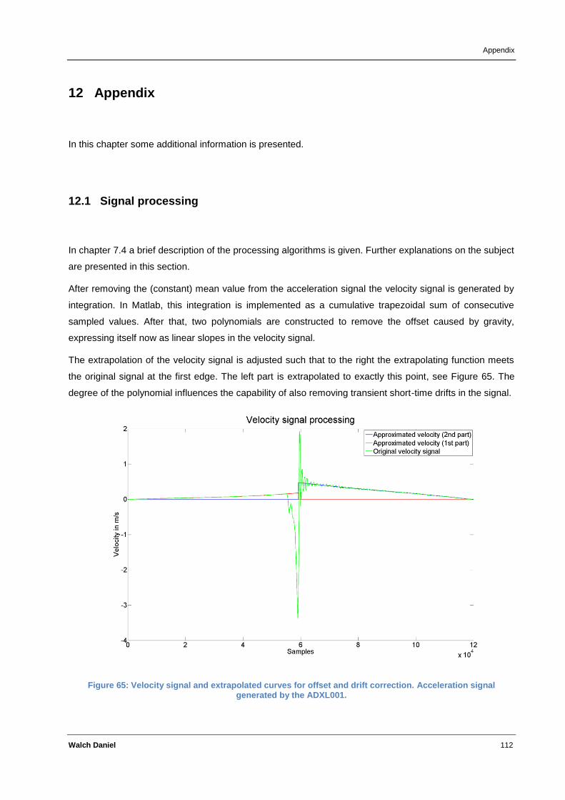
Appendix
Walch Daniel 112
12 Appendix
In this chapter some additional information is presented.
12.1 Signal processing
In chapter 7.4 a brief description of the processing algorithms is given. Further explanations on the subject
are presented in this section.
After removing the (constant) mean value from the acceleration signal the velocity signal is generated by
integration. In Matlab, this integration is implemented as a cumulative trapezoidal sum of consecutive
sampled values. After that, two polynomials are constructed to remove the offset caused by gravity,
expressing itself now as linear slopes in the velocity signal.
The extrapolation of the velocity signal is adjusted such that to the right the extrapolating function meets
the original signal at the first edge. The left part is extrapolated to exactly this point, see Figure 65. The
degree of the polynomial influences the capability of also removing transient short-time drifts in the signal.
Figure 65: Velocity signal and extrapolated curves for offset and drift correction. Acceleration signal generated by the ADXL001.
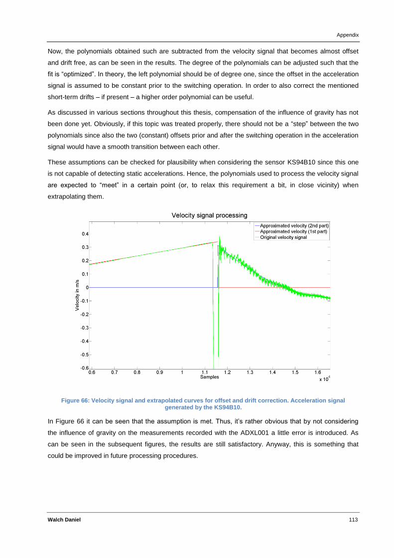
Appendix
Walch Daniel 113
Now, the polynomials obtained such are subtracted from the velocity signal that becomes almost offset
and drift free, as can be seen in the results. The degree of the polynomials can be adjusted such that the
fit is “optimized”. In theory, the left polynomial should be of degree one, since the offset in the acceleration
signal is assumed to be constant prior to the switching operation. In order to also correct the mentioned
short-term drifts – if present – a higher order polynomial can be useful.
As discussed in various sections throughout this thesis, compensation of the influence of gravity has not
been done yet. Obviously, if this topic was treated properly, there should not be a “step” between the two
polynomials since also the two (constant) offsets prior and after the switching operation in the acceleration
signal would have a smooth transition between each other.
These assumptions can be checked for plausibility when considering the sensor KS94B10 since this one
is not capable of detecting static accelerations. Hence, the polynomials used to process the velocity signal
are expected to “meet” in a certain point (or, to relax this requirement a bit, in close vicinity) when
extrapolating them.
Figure 66: Velocity signal and extrapolated curves for offset and drift correction. Acceleration signal generated by the KS94B10.
In Figure 66 it can be seen that the assumption is met. Thus, it’s rather obvious that by not considering
the influence of gravity on the measurements recorded with the ADXL001 a little error is introduced. As
can be seen in the subsequent figures, the results are still satisfactory. Anyway, this is something that
could be improved in future processing procedures.

Appendix
Walch Daniel 114
12.2 Field test in Werben
The first and yet last test of the measurement system in the field was carried out in a power distribution
station in Werben, Vorarlberg. All three sensors described in chapter 7.1 were tested. Prior knowledge
about the device under test, namely a SF6 high voltage circuit breaker by Areva (model GL314 220 kV),
was available due to the work of Sylvia Hämmerle within her Bachelor thesis. The main information
concerned the attachment possibilities, where the mechanical relations at an axle of the CB are
described. By knowing the mechanical relations it was possible to construct adapter pieces for convenient
mounting onto the CB. The adapter pieces itself contained the sensors.
Figure 67: Geometrical relations at the shaft of the HVCB, not to scale [71].
Exploiting this information, the construction of two adapter pieces was carried out with support of an
Omicron employee who drew the mechanical sketches before “constructing” them with a 3D printer,
located at Omicron electronics.
The following pictures (Figure 68, Figure 69, and Figure 70) show the adapter pieces mounted to the axle
with the sensors attached.
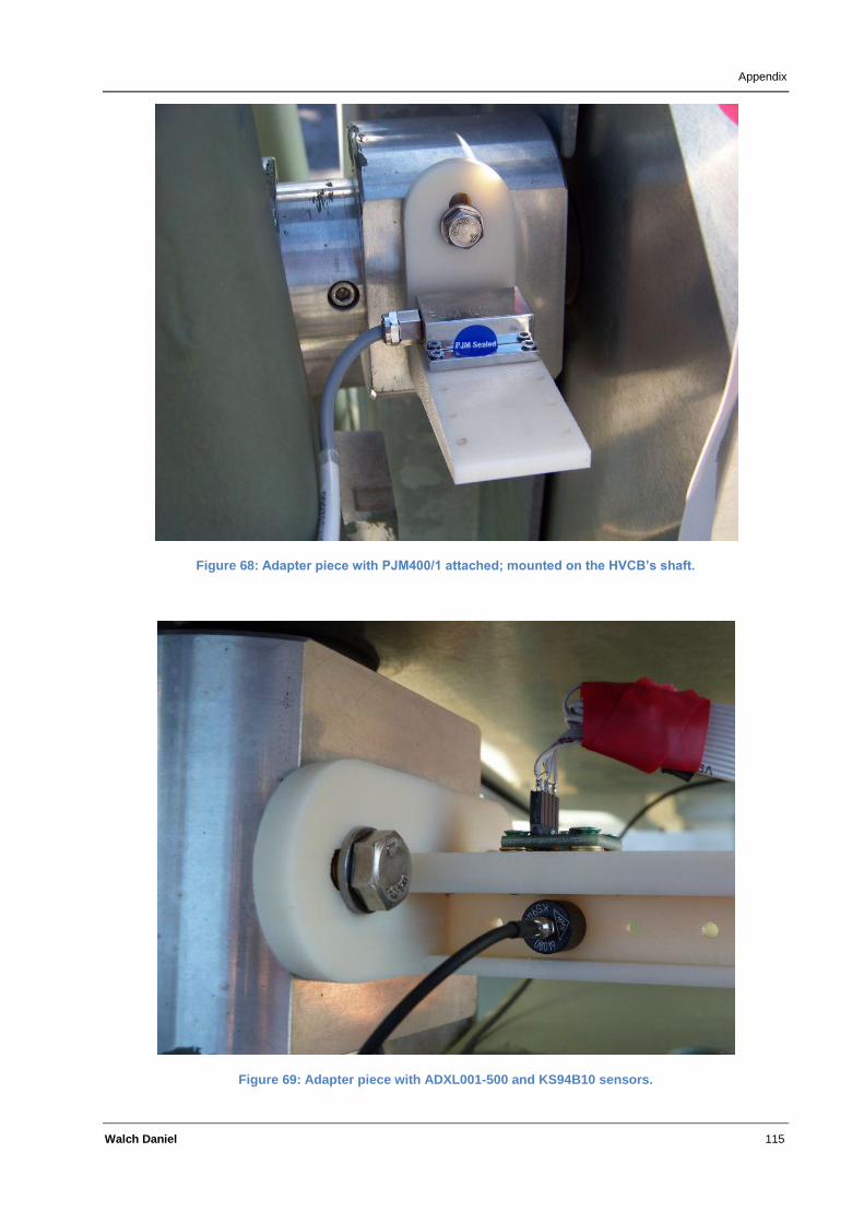
Appendix
Walch Daniel 115
Figure 68: Adapter piece with PJM400/1 attached; mounted on the HVCB’s shaft.
Figure 69: Adapter piece with ADXL001-500 and KS94B10 sensors.

Appendix
Walch Daniel 116
Obviously, all sensors in this test series travel on an arc segment. Again, as for all the other measurement
series, the problem is that the influence of gravity has not yet been taken into account. As a result, the
absolute displacement information will vary between switching “ON” and “OFF” operations. In order to
improve the results, the influence of gravity during the switching operation should be considered and the
results be compensated.
In addition to the two sensors that are depicted in Figure 69, another ADXL001 sensor was applied to the
HVCB’s housing to record vibrations caused by the switching operations (Figure 70).
Later on it turned out that this additional information cannot (easily) be used to improve the results.
Figure 70: Additional ADXL001 sensor attached to the housing of the HVCB to measure the vibrations of the whole HVCB.
The ADXL001 mounted onto the adapter piece was terminated with a 47 Ω resistor and a 1 nF capacitor.
Together with the 2.2 nF capacitor of the evaluation board of the ADS1274 it forms a lowpass filter with a
relatively high cutoff frequency compared to the sensor’s resonant frequency.
The ADXL001 mounted onto the housing of the HVCB has no additional circuitry at its output. Both
sensors were attached to the ADC evaluation board with approximately 6 m long cables.
The KS94B10’s output has to be transformed to meet the requirements of the ADC input. The AD8275 16-
Bit ADC Driver by Analog Devices was used to adjust the KS94B10’s output signal to the input range of
the ADC (+/-VREF). The circuit was built up such that the signal with a DC offset of approximately 13V
(operating point of the sensor) with the acceleration signal oscillating around it was divided by 5 and then
level-shifted to 2.5V DC. This guaranteed that the ADC’s inputs would not suffer from possible
overvoltage.
The circuitry is shown below. Two additional components are drawn that have not been applied during the
test series: the analog integrator stage and the impedance converter.
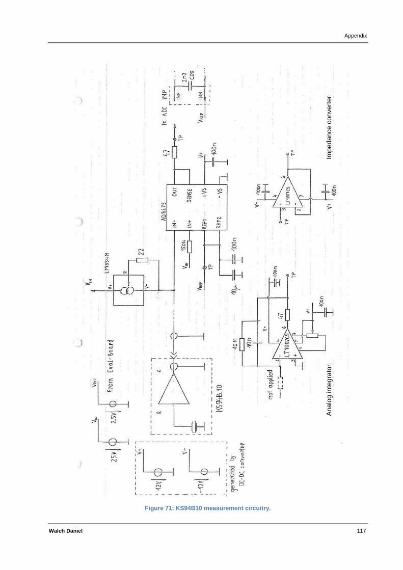
Appendix
Walch Daniel 117
Figure 71: KS94B10 measurement circuitry.
Impe
dance c
onvert
er
Ana
log inte
gra
tor
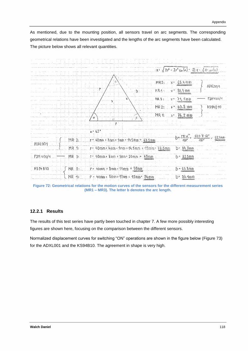
Appendix
Walch Daniel 118
As mentioned, due to the mounting position, all sensors travel on arc segments. The corresponding
geometrical relations have been investigated and the lengths of the arc segments have been calculated.
The picture below shows all relevant quantities.
Figure 72: Geometrical relations for the motion curves of the sensors for the different measurement series (MR1 – MR3). The letter b denotes the arc length.
12.2.1 Results
The results of this test series have partly been touched in chapter 7. A few more possibly interesting
figures are shown here, focusing on the comparison between the different sensors.
Normalized displacement curves for switching “ON” operations are shown in the figure below (Figure 73)
for the ADXL001 and the KS94B10. The agreement in shape is very high.
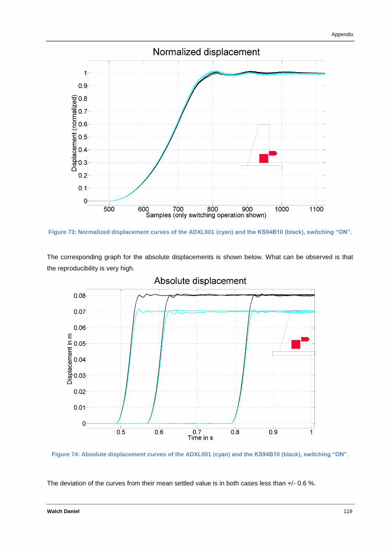
Appendix
Walch Daniel 119
Figure 73: Normalized displacement curves of the ADXL001 (cyan) and the KS94B10 (black), switching “ON”.
The corresponding graph for the absolute displacements is shown below. What can be observed is that
the reproducibility is very high.
Figure 74: Absolute displacement curves of the ADXL001 (cyan) and the KS94B10 (black), switching “ON”.
The deviation of the curves from their mean settled value is in both cases less than +/- 0.6 %.
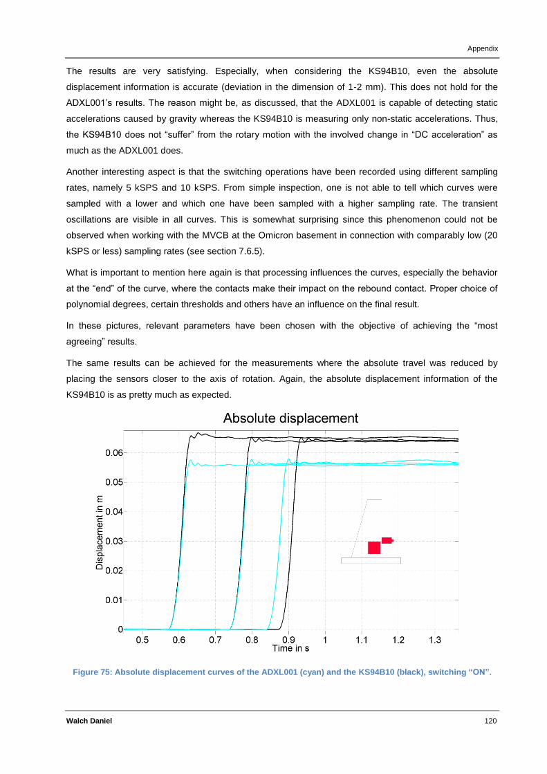
Appendix
Walch Daniel 120
The results are very satisfying. Especially, when considering the KS94B10, even the absolute
displacement information is accurate (deviation in the dimension of 1-2 mm). This does not hold for the
ADXL001’s results. The reason might be, as discussed, that the ADXL001 is capable of detecting static
accelerations caused by gravity whereas the KS94B10 is measuring only non-static accelerations. Thus,
the KS94B10 does not “suffer” from the rotary motion with the involved change in “DC acceleration” as
much as the ADXL001 does.
Another interesting aspect is that the switching operations have been recorded using different sampling
rates, namely 5 kSPS and 10 kSPS. From simple inspection, one is not able to tell which curves were
sampled with a lower and which one have been sampled with a higher sampling rate. The transient
oscillations are visible in all curves. This is somewhat surprising since this phenomenon could not be
observed when working with the MVCB at the Omicron basement in connection with comparably low (20
kSPS or less) sampling rates (see section 7.6.5).
What is important to mention here again is that processing influences the curves, especially the behavior
at the “end” of the curve, where the contacts make their impact on the rebound contact. Proper choice of
polynomial degrees, certain thresholds and others have an influence on the final result.
In these pictures, relevant parameters have been chosen with the objective of achieving the “most
agreeing” results.
The same results can be achieved for the measurements where the absolute travel was reduced by
placing the sensors closer to the axis of rotation. Again, the absolute displacement information of the
KS94B10 is as pretty much as expected.
Figure 75: Absolute displacement curves of the ADXL001 (cyan) and the KS94B10 (black), switching “ON”.
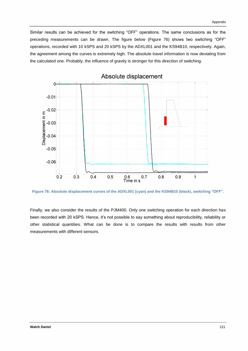
Appendix
Walch Daniel 121
Similar results can be achieved for the switching “OFF” operations. The same conclusions as for the
preceding measurements can be drawn. The figure below (Figure 76) shows two switching “OFF”
operations, recorded with 10 kSPS and 20 kSPS by the ADXL001 and the KS94B10, respectively. Again,
the agreement among the curves is extremely high. The absolute travel information is now deviating from
the calculated one. Probably, the influence of gravity is stronger for this direction of switching.
Figure 76: Absolute displacement curves of the ADXL001 (cyan) and the KS94B10 (black), switching “OFF”.
Finally, we also consider the results of the PJM400. Only one switching operation for each direction has
been recorded with 20 kSPS. Hence, it’s not possible to say something about reproducibility, reliability or
other statistical quantities. What can be done is to compare the results with results from other
measurements with different sensors.
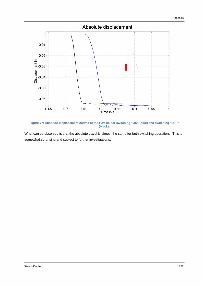
Appendix
Walch Daniel 122
Figure 77: Absolute displacement curves of the PJM400 for switching "ON" (blue) and switching "OFF" (black).
What can be observed is that the absolute travel is almost the same for both switching operations. This is
somewhat surprising and subject to further investigations.

Acknowledgements
Walch Daniel 123
Acknowledgements
"Für den gläubigen Menschen steht Gott am Anfang, für den Wissenschaftler am Ende aller seiner
Überlegungen."
- Max Planck
Lob und Preis dem Schöpfer von Himmel und Erde und meinem persönlichen Erlöser.
Liebe Julia, du bist der wichtigste Mensch in meinem Leben. Ich danke dir für deine Liebe, dein
Verständnis und deine Vergebung und dass du immer für mich da bist. Ich liebe dich.
Danke an meine Freunde und Klassenkameraden, welche mir in der Schulzeit den Alltag lustiger,
abwechslungsreicher und spannender gemacht haben, im Speziellen René, Daniel und Simon.
Andi + Evi, Matze + Karo, Oskar + Manu, Michi + Babs: ihr seid wahre Freunde.
Johannes, Jens und Dominik – es war lässig, mit euch studieren zu dürfen. Danke für die Unterstützung
und Geduld mit meinen anstrengenden Eigenschaften und für die vielen Stunden in relaxter Atmosphäre.
Werte Professoren, Anerkennung an diejenigen von euch, die ihr mit Leidenschaft und Engagement
jungen Leuten euer Wissen vermittelt trotz der Unzulänglichkeiten eures Umfelds.
Ein großes Dankeschön an meine lieben Eltern. Danke, dass ihr mich im Glauben erzogen habt, mir eine
gute Ausbildung ermöglicht habt und mir eine unbeschwerte Kindheit beschert habt. Liebe Geschwister
und Verwandte, danke dass ihr mich zu dem gemacht habt was ich heute bin.
Liebe Familie Zoderer, danke für die Aufnahme unter euer Dach für ein paar Jahre und dafür, dass ihr
stets mit Rat und Tat beiseite gestanden habt und für die schönen Erlebnisse.
Geschätzte Arbeitskollegen, ihr seid mir bei Fragen immer gern zur Verfügung gestanden – vielen Dank,
insbesondere an Reini.
Herr Prof. Zangl, vielen Dank für die Betreuung meiner Arbeit und die unbürokratische Abwicklung der
organisatorischen Dinge trotz der räumlichen Entfernung.
Danke an die Leute in meiner Heimatgemeinde – ihr helft mir, das Ziel im Auge zu behalten.
An die Künstler und Musiker, die es mir leichter gemacht haben, zu später Stunde wach zu bleiben:
danke.
Liebe Sport- und Tenniskollegen: danke für die Gesellschaft und die Leidenschaft für unseren Sport.
Ohne euch wäre ich weniger ausgeglichen und wahrscheinlich dicker.
Danke an alle, die mir wichtig sind aber hier nicht namentlich erwähnen kann, dass ihr mir nicht böse
dafür seid.
Related Documents