Discussion paper No. 58 - esri.cao.go.jp

Discussion paper No. 58

Asset Market and Business Fluctuations in Japan

by

Kazuo Ogawa

Kobe University

Economic Planning Agency

and

Shin-ichi Kitasaka

Nagoya City University

Economic Planning Agency

December 1993

Economic Research Institute

Economic Planning Agency

Tokyo, Japan

Asset Market and Business Fluctuations in Japan*

Kazuo Ogawa 1)

Shin-ichi Kitasaka 2)

Toshio Watanabe 3)

Tatsuya Maruyama 4)

Hiroshi Yamaoka 4)

Yasuharu Iwata 4)

* Early version of this paper was presented at the Tenth International Symposium held at the

Economic Research Institute, Economic Planning Agency on March 24-25, 1993 and the

workshop at the Japan Development Bank. We are grateful to Kazumi Asako, Kazumasa Iwata,

Morio Kuninori, Tsutomu Miyagawa, Syuji Nishijima, Kazuyuki Suzuki, Yosuke Takeda, and

Hiroshi Yoshikawa for extremely helpful comments and suggestions. All remaining errors are,

of course, our own.

1) Kobe University and Economic Research Institute, Economic Planning Agency

2) Nagoya City University and Economic Research Institute, Economic Planning Agency

3) Toho Life Insurance

4) Economic Research Institute, Economic Planning Agency

－1－

1.Introduction

The Japanese economy has plunged into deep recession around the fourth quarter of 1990 to

the first quarter of 1991 after a long period of booms, which is recorded as the second longest

booms in the postwar period in Japan. The real GNP growth rates hovered around 5 % during the

fiscal years of 1987-1991, while it was only 1.5 % in 1992. Among the demand components,

slowdown of growth is observed most notably for the private residential investment and business

investment. The growth rate of the former was -8.6 % and -5.4 % in 1991 and 1992, while that of

the latter was -4.1 % in 1992.

However, the most notable characteristics in the current recession can be seen in the asset

markets, especially in the stock market and the land market. The Tokyo Stock Exchange Price

Index (TOPIX) precipitated in January of 1990 after a long spell of price soaring in the preceding

boom periods. The TOPIX declined by 57.8 % from December of 1989, peak of the stock price, to

August of 1992. The land price exhibited a similar pattern. The land price index of six largest cities

rose at the rate of 24.5 % per annum from September of 1985 to September of 1990 ,which was

followed by a sharp decline. Many corporations which were given loans by the financial

institutions on the security of land and stocks during the boom periods have become insolvent and

some argue that it will lead to an instability of the financial system in Japan.

Thus there seems to be financial factors in addition to real factors such as insufficient level of

effective demand underlying the current recession. That is why the current recession is often called

"complex " depression. 1)

The purpose of this paper is to investigate the roles played by the asset markets in the recent

business cycle. As is stated above, the asset prices, in particular the stock price and the land price,

showed an excessive fluctuations during the current business cycle. In the first place we will

analyze whether the stock price fluctuations during the mid-80's to the early 90's were caused by a

change of the fundamentals underlying the Japanese economy. If the answer to that question is no,

then we pose the question: how did the divergence of the prices from the fundamentals affected the

behavior of the economic agents ? We tackle this problem by investigating the portfolio behavior

of the corporate sector.

Secondly we will examine the effects of the market value of land held by the corporate sector

on the business fluctuations. In particular we are interested in the role of land asset as a collateral.

This aspect is analyzed by including the market value of land as one of the explanatory variables in

the portfolio equations of the firm.

Let us summarize our main findings: 1) The stock prices diverged from the fundamentals to a

large extent from the mid-80's to the early 90's. That is to say, it is highly likely that there existed

bubbles in the stock market. Another finding is that the corporations responded differently to the

change in the fundamentals and the bubbles. The bubbles turned out to exert a negative effect on

－2－

the portfolio behavior of the corporations such as real investment, land purchase, and borrowings.

2) The land stock played an active role as a collateral in the portfolio behavior of the

corporations. We obtained some evidence that a rise in land prices increased the value of land as a

collateral and hence led to an increase of the real investment and borrowings of the corporations.

The importance of land stock as a collateral was reinforced by two factors: the financial

liberalization under way in the early to the middle of 80's and a rise in the stock prices. These

factors enabled large companies to raise the funds directly from the capital market by issuing

equity or bonds, which in turn prompted the financial institutions to lend to the corporations that

did not have direct access to the capital markets. The banks had not established the long-term,

stable relationship with these corporations. Therefore the land asset held by the corporations,

which was increasing in value at that time, played a collateral role and eased the agency costs

arising from the information asymmetries between creditors and debtors. The loans received were

then channeled toward the real investment and the financial investment.

3) The dependence of real activities such as investment on the asset prices works as

amplifying the magnitude of the business cycle, since the asset prices move procyclically. The

severity of the recession the Japanese economy has experienced results from this very dependence

of real activities on the asset markets. The precipitation of the asset prices in the early 90's stripped

off the collateral value of the assets held by the corporations and the deteriorating loans made the

financial institutions quite cautious in further lending and it choked off the investment to a large

extent.

The paper is organized as follows. Section 2 detects the characteristics intrinsic to the current

recession and the preceding booms by comparing the current business cycles with those in the past.

Section 3 and 4 analyze the roles played by the asset markets in the current business cycles. The

effect of the asset prices on the portfolio behavior of the corporations are examined quantitatively

in Section 5. Section 6 gives concluding remarks.

2.Characteristics of the Contemporary Business Cycles

In this section we first identify the macroeconomic characteristics pertinent to the current

recession and the preceding booms by comparing the current business cycles with those in the past.

Then light is shed on the micro aspects of the business cycles: changes in the financial structure of

the corporations.

The key statistics characterizing the business cycles since 1958 are summarized in Table 1

and 2 for boom periods and recession periods, respectively. From Table 1 we can pick up several

points characterizing the second longest booms starting from November in 1986. First, the growth

rate of private fixed and residential investment was quite high. The growth rate of both types of

investment exceeded 10 %, which almost equaled that in the galloping growth period in the 60's.

－3－

Second the asset prices such as land and stocks increased rapidly at the rate of around 20 %

per annum during this boom, while the prices of goods and services represented by the GNP

deflator were quite stable. In the boom periods in the 60's the asset prices also soared, but the

prices of goods and services also increased at the rate of more than 5 %. The high level of asset

prices generated the expectation of further increase of asset prices in the future and it led to an

increase of the demand for assets. Figure 1 shows the purchases of the share and the land by the

different sectors. The demand for shares increased during 1985-1989 mainly among the financial

institutions, while the demand for land by the nonfinancial corporations increased from 1986 to

1990.

The third point, which is related to the second, is that the credit conditions were quite eased.

The growth rate of M2+CD exceeded 10 % per annum and the historically low levels of the interest

rates emerged. The discount rate was cut stepwise from the level of 4.5 % in January of 1986 to

2.5 % in February of 1987, lowest level in the the postwar period.

Next we turn to the characteristics of the recessions the Japanese economy is in the middle of.

From Table 2 we point out the following characteristics, most of which are related to the

conditions in the financial markets. First the growth rate of investment was reduced to a large

extent. Second the asset prices declined by 20.3 % (shares) to 9.7 % (land). Third the growth rate

of money supply was lowest (3.01 %) in the postwar recessions. The conditions in the financial or

asset markets during the current recession are quite contrasted with those in the preceding booms.

The easy credit conditions in the booms are completely reversed to the tight conditions as the asset

prices started to decline.

The financial structure of the nonfinancial corporations also changed in the course of the

financial liberalization under way. First the issue of the bonds with warrants was approved in 1981.

During the period of 1986 to 1989, the corporations raised the funds to a large extent by issuing

the bonds with warrants and the convertible bonds under the expectations that the share prices will

rise. During this time the equity issue also increased due to high stock prices. The average annual

growth rate of the amount raised by the warrant bonds, convertible bonds, and equity for the

corporations listed in all the stock exchanges in Japan are 64.8 %, 38.8 %, and 116%, respectively.

However, the bond-financing or equity-financing was not uniformly prevalent across all the

corporations. It was restricted only to the large corporations which could have direct access to the

capital markets. Figure 2 shows the time-series pattern of the ratio of equity capital to liabilities

plus equity capital for the corporations of different sizes in six industries: all industries,

manufacturing, construction, wholesale and retail trade, services, and real estate. The ratio of

equity capital increased steadily over time for all industries, manufacturings, and wholesale and

retail trade. However the increasing trend is only observed for the corporations in the category of

largest size. This is typically seen for the large corporations whose capital stock is larger than one

－4－

billion yen. Figure 4 shows the time-series pattern of the ratio of equity capital to liabilities plus

equity capital for the corporations whose capital stock is larger than one billion yen for all

industries and manufacturing. The ratio increased steadily from 16.8 % (19.9 %) in 1974 to 26.4 %

(36.4 %) in 1990 for all industries (manufacturing).

The second feature, which is related to the first, is the less dependence on borrowings for the

large corporations on one hand, and the more dependence on borrowings for the medium or small-

sized corporations on the other hand. Figure 3 shows the time-series paths of the dependence on

borrowings of the corporations measured by the ratio of outstanding loans payable to sales.

The dependence on borrowings are mitigating over time for the largest corporations in

manufacturing and construction industries. This tendency is especially notable for manufacturing.

This is also seen in Figure 4, where the ratio of outstanding loans to sales are depicted for the

corporations whose capital stock is larger than one billion yen. This ratio declined from 32.6 %

(42.7 %) in 1975 to 22.7 % (15.2 %) in 1990 for all industries (manufacturing). Figure 5 shows

that this change in the structure of the corporate finance is also observed in flow terms. In Figure 5

the proportions of equity issue, borrowings, and corporate bonds in the total demand for credit of

the corporations whose capital stock is larger than one billion yen are depicted over time. The

proportion of borrowings are constantly declining. For manufacturing the ratios are even negative

during 1983-1989. On the other hand the proportion of equity issue and bonds are notably high

during 1985-1989.

Figure 3 also shows that the dependence on borrowings has increased over time for the rest of

the corporations. The dependence has increased even for the largest corporations in wholesale and

retail trade, services, and real estate. We will examine below how a shift of financing from

borrowing to equity or bond issuing among the large corporations affects the pattern of business

fluctuations.

The third feature of a change in the financial structure of the corporations is an increase of the

holdings of liquid assets such as cash, time deposits and short-term securities in the late 80's. This

is demonstrated in Figure 6, where the movements of the ratio of liquid assets to sales are given. It

can be seen from the figures that this liquidity ratio increased during 1986 to 1989 for all the

industries but real estates, irrespective of the size of the corporations. For real estates the ratio

started to rise in 1984, reaching its peak in 1986.

There existed two underlying conditions leading to a rise in the liquidity ratios. One is

deregulations on the level of the interest rates on time deposits, which was initiated in March of

1985 as an approval of money market certificate(MMC) and followed by a sequence of the

liberalization of the interest rates earned on the time deposits of a large lot. The stock of time

deposits including certificates of deposits held by the corporations increased at the rate of 16.0 %

per annum from 1984 to 1989, while that of the households increased only at the rate of 7.8 % per

－5－

annum. The other is the low interest rates charged on loans during this period. It enabled the

corporations to earn large margins by depositing the money borrowed from the banks. A

simultaneous operation of borrowing and depositing by the corporations contributed to a creation

of credits by raising the magnitude of the credit multiplier.

3. Role of Asset Markets in Business Cycles: (1) Collateral Role of Assets

We discuss the roles played by the asset markets in business cycles. In particular our interest

lies in whether the increasing weight given on the asset market in the economy magnifies the

business fluctuations or not. In general the asset prices fluctuate more than the real variables, as is

typically observed in the current recession and the preceding booms. The problem is whether the

volatility of asset markets is propagated to the real economy. If the answer is yes, then much of the

current business fluctuations are attributed to those in the asset prices. We discuss this problem

from two viewpoints. One is the collateral role played by the asset values, especially land value.

The other is a signaling role played by the stock market. In this section we discuss the first problem

and the second one will be dealt with in the next section.

According to the celebrated Modigliani-Miller theorem, There exists no difference in cost

between the internal funds and the external funds and therefore the level of investment is

independent of the financing method. However doubt has been cast on the validity of the

fundamental assumptions underlying the theorem since the theorem came into being. The

assumption of perfect information has been often criticized as unrealistic and growing attention

has been paid to an alternative assumption of the asymmetric information between creditors and

debtors. It is quite natural to assume that the corporations as a borrower has superior information

on the investment projects to be undertaken to lenders. Furthermore the lenders cannot monitor the

behavior of the borrowers perfectly without incurring additional costs. Then there arises the well-

known principal-agent problem. In those situations the optimal financial arrangements will be

made between the lenders and the borrowers that include the clauses that prevent the borrowers

from taking actions disadvantageous to the lenders. However it is demonstrated that the level of

investment by the corporations becomes inefficient compared to that without any informational

friction due to the costs arising from the financial arrangements.

This cost drives the wedge between the cost of internal funds and that of the external funds.

The upshot is that the investment decision is no longer independent of the method of raising funds.

The cost of internal funds is cheap relative to that of external funds. Therefore the abundance of

internal funds induces the corporations to undertake more investment projects. Recently this

argument is further elaborated and it is shown that what reduces the agency costs is the

collateralizable net worth of the borrowers. In other words the information regarding the balance

sheets of the debtors plays a vital role in determining the level of investment. 2) The larger the

－6－

collateralizable net worth is, the higher the level of investment is. Emphasis on the net worth in

investment decision has important implications to the business fluctuations. Combining the fact

that the asset prices move procyclically with the positive dependence of investment on the level of

collateralizable net worth, it can be deduced that the fluctuations of investment will be magnified

and thus the volatility of business cycles will be amplified.

Hoshi,Kashyap, and Scharfstein(1990,1991), Asako, Kuninori, Inoue, and Murase(1990), and

Okazaki and Horiuchi(1992) investigated the validity of this theory for Japan based on the firm

data. It is well-known in Japan that there are industry groups called keiretsu. The corporations

belonging to industry groups can mitigate the agency costs for several reasons. First group corpo-

rations have close ties with affiliated banks and those banks are shareholders as well as

bondholders, which reduces the conflicts among investors. Second group corporations have a long-

term stable relationship with the affiliated banks and former bank employees are often placed in

management positions of the corporations, which narrows the informational gaps between the bank

and the corporations. Therefore it is expected that the agency cost is lower for the corporations in

the industry groups than unaffiliated corporations. Hoshi et al.(1990,1991) obtain evidence

supporting this conjecture, while the evidence given by Asako et al.(1990) and Okazaki and

Horiuchi(1992) is not so decisive.

If the assertions made above are correct, then we have strong implications on the role of assets

as a collateral in business cycles. In the preceding session we gave some evidence that financial

liberalization together with a rise of share prices in the middle of 80's shifted the source of

financing for the large corporations from borrowing to equity or bonds and that the dependence on

borrowings was strengthened for medium and small corporations which cannot have direct access

to the capital market. In general the corporations of medium or small size do not belong to industry

groups and hence the banks have not accumulated the enough information of those corporations on

which judgment is made as to the decision of lending loans. However the asset values held by the

corporations increased to a large extent in the middle of 80's due to a sharp rise in asset prices. It is

conjectured that appreciating assets played a collateral role in borrowing and that it eased the

agency costs. If it is the case, then the improvement of the balance sheet positions of medium or

small corporations were indispensable to credit expansions and high growth rate of the investment

during this period.

Now we turn to the evidence on our assertions. First we demonstrate from the statistics of the

supplier of funds that the loans made for the small corporations indeed had the tendency to

increase in the 80's. Figure 7 depicts the share of the small enterprises in the total outstandings of

loans and discounts of all banks in Japan. The share is increasing over time and it accelerated from

the middle of 80's to 1989. Figure 8 shows the proportions of the loans outstandings that are on the

security of real estates and securities, respectively. The proportion of loans on the security of real

－7－

estates declined rapidly from the middle of 70's to the middle of 80's and switched to an

increasing trend. The proportion of loans the collateral of which is securities exhibits a similar

pattern. It showed a continuous decline from the middle of 60's to the middle of 80's and the

declining trend was reversed to an increasing one. Note that the increasing trend of both

proportions coincide with the period of sharp rise in land and share prices.

To establish empirically the relationship between the proportions of collateral loans and the

share of small enterprises in loan outstandings, the following regressions were run. 3)

(1) SCOL ＝ 0＋( ＋ TOPIXHAT )SMALL ＋ SCOL

(2) LCOL ＝ ＋( ＋ PLANDHAT )SMALL ＋ LCOL

where SCOL : proportion of loan outstandings of all banks secured on securities

LCOL : proportion of loan outstandings of all banks on the security of land

TOPIXHAT: rate of increase of Tokyo Stock Exchange price indexes(TOPIX),

computed as (TOPIX/TOPIX -1 -1 )

PLANDHAT: rate of increase of land price indexes of six largest

cities(PLAND), computed as (PLAND/PLAND -1 -1 )

SMALL : share of small enterprises in the outstandings of loans

The regressions are run for the period of 1978-1991. The results are shown in Table 3. The SMALL

coefficient is positive for both the SCOL and the LCOL equations and that it is significant at the

1 % level for the latter case. The cross term of the SMALL variable with the rate of return is also

positive in both equations and it is significant at the 1 % level for the SCOL equations. 4) Our

evidence shows that as the banks shifted the weight of loans to small enterprises, the proportion of

loan outstandings on the security of land and securities increased. Furthermore the proportion of

loan outstandings on the security of assets becomes more responsive to the share of small

enterprises in the total outstandings of loans as the rate of change in asset prices increases. More

detailed analysis of the effects of the land value on investment and borrowings will be made in the

next section by using industry data.

4. Role of Asset Markets in Business Cycles: (2) Valuation in the Stock Market and Business

Fluctuations

One of the fundamental functions of the stock market is to reflect a high quality of information

of the corporation on the stock price. In addition to this basic property of the stock market, if the

marginal prospects of corporate investment is equal to the average profitability of the existing

－8－

capital stock, then the average q ratio, defined as the ratio of the firm value evaluated at the

financial market to the replacement value of the physical capital, is a sufficient statistics of

investment. 5) The upshot is a high positive correlation of investment with the average q and the

investment is as volatile as the average q, which reflects the fluctuations in the stock market.

As is seen in the previous sections, the stock market in the Japanese economy soared in the

middle of 80's and precipitated in 1990. Some argue that there existed some components of

bubbles or fads which forced the stock prices to deviate from the fundamental parts, and it burst in

1990. If it is the case, then the question to be posed is : does the manager still pay attention

to the signals from the stock market even if the stock price deviates from the fundamentals that

reflect the prospects of the investment perceived by the managers ? 6) If it turns out that the

managers do not care about the valuations in the stock market, then the investment will be less

volatile than the stock price. 7) Therefore the answer to this question is very crucial in assessing

the role of asset markets in business fluctuations.

We tackle this tough, but important problem empirically. First we construct the proxy of the

marginal profitability of investment, fundamental parts of the stock price and compare that proxy

with the market valuation of the corporation, that is, average q. Then if the evidence is against the

efficiency hypothesis that the stock price does not deviate from the fundamentals, we will examine

how the response of the managers to the fundamentals and to the non-fundamentals differs.

Now explanations are in order for the data set employed. Based on the Quarterly Report of

Financial Statements of Incorporated Business compiled by the Ministry of Finance, we construct

the consistent quarterly series of the major items in the balance sheet of the corporations for each

industry. 8) The sample period covers from the third quarter of 1968 to the third quarter of 1992.

The detailed explanations on the procedures of the data construction are provided in Data

Appendix.

First we compute the tax-adjusted average q, average profitability of the capital. As for the

definition of capital, we include only depreciable assets in the definition of capital. This definition

excludes financial assets, inventories, and land from capital. 9) Specifically, our average q is

defined as follows: 10)

(3) ＋ － －

(1－ )(1－ )

where : market value of equity

Bt-1 : net financial liability at the end of period t-1

: expected present value of tax savings on the depreciation allowances on

investment made before period t

－9－

: land price

Lt-1 : real stock of land at the end of period t-1

: physical depreciation rate

: investment goods price

Kt-1 : real capital stock at the end of period t-1

: expected present value of current and future investment allowances on a unit of

investment expenditure in period t

The fundamental part of the stock price is proxied by the present discounted value of arginal

profitability of investment divided by the investment goods deflator. This is tax-adjusted marginal

q and it is defined as:

(4) MAQ ＝ 1

(1－ ) (1－ ) (1－ )

where ＝ (1＋ ) ( ＝1,2,…) , ≡1

rt+1 : one-period nominal discount rate in period t

: corporate tax rate

: before-tax profits divided by the real capital stock

[+]: mathematical expectation operator conditional upon the information available

in period t

In deriving eq.(4) we assume the technology of constant return to scale. Then the use of average

profit rates as the marginal profits can be justified. The marginal q is not directly observable since

it includes the unobservables: future stream of discount rates and profit rates. Therefore to make

eq.(4) operational we have to know the stochastic structure underlying the discount factor and

profit rates. 11) As a first step to pinpoint the stochastic process we test whether the discount

factor (= (1- )/(1+r )) and profit rates have unit roots. Two types of unit root tests are

conducted. One is the Augmented Dickey Fuller test(ADF test) and the other is Phillips-Perron

test. 12) The null hypothesis is chosen as one unit root without trend for the discount factor and

one unit root with trend for the profit rates. Technical progress may have some effect on the level

of profit rates, which will justify our allowance for trend in the case of profit rates. The lag length

is chosen to be 4 in both types of tests. The results of unit root tests are presented in Table 4. As

for the discount factors, we cannot reject the null hypothesis for any industries, while for the profit

rates the unit root is decisively rejected at the 1 % significance level for all the industries by the

j

i＝1 Π

∞

j＝0 Σ

－10－

Phillips-Perron test. It implies that the movement of profit rates are better characterized by trend

stationary process.

Based on the test results, we specify the stochastic process of the discount factors and the

profit rates as follows: 13)

(5) Δ ＝ ＋ Δ ＋

(6) ＝ ＋ ＋ ＋

where t : time trend

, : white noise

The lag lengths of eqs.(5) and (6) are determined on the basis of Schwarz Information Criterion,

which are shown in Table 5. The lag length of one is chosen for both the discount factors and the

profit rates in all the industries but construction. Table 6 shows the estimation results of eqs.(5)

and (6) based on the lag length chosen above.

When the stochastic process of and is characterized by eqs.(5) and (6), it can be shown

that the tax-adjusted marginal q is written as: 14)

(7) MAQ ＝

(I－ M ) M ＋

(I－ M ) (1－ ) (1－ )

＋ (I－ M ) M ＋1

(I－ M ) (1－ )

＋

＋ 1

(I－ M ) n](1－ )

(1－ ) (1－ ) (1－ )

where ＝(1,0,…,0)

＝(Δ ,Δ ,…,Δ )

＝( ,0,…,0)

＝( , ,…, )

＝( ,0,…,0) ＝( ,0,…,0)

p

k＝1 Σ

q

k＝1 Σ

－11－

We use the ratio of operating profits to the real capital stock as a proxy ofπ. Before examining the

relationship between the market valuation and the fundamentals, we give some summary statistics

on the AVQ and the MAQ variables.The mean and standard deviation are computed for the period

of the first quarter of 1970 to the fourth quarter of 1990. They are shown in Table 7. The

magnitude of the AVQ variable is reasonable for all industries, manufacturing, construction, while

that of the MAQ variable is reasonable for all industries, manufacturing, and real estate. The

average q is negative for real estate, and it seems that the AVQ and the MAQ variables are

overestimated for wholesale and retail trade. It should be noted that the AVQ variables are more

volatile than the MAQ variables across all the industries in the sample. In fact the standard

deviation of the former is 2.37 to 5.88 times as large as the latter(third column of Table 7).

Now we examine the relationship of the fundamentals with the market valuations. If the stock

price reflects all the relevant information on the future profitability of investment projects

undertaken by the firm, then the AVQ variable will be equal to the MAQ variable. Once both series

of the AVQ and the MAQ variables are constructed, it is easy to test equality between two series.

Taking the sampling errors into consideration, the null hypothesis is written as follows:

(8) AVQ ＝ MAQ ＋u

where u :sampling error uncorrelated with the MAQ variable

Eq.(8) can be tested in several ways. The simplest way to test eq.(8) is to estimate the following

equation and test the hypothesis that = 0 and = 1.

(9) AVQ ＝ ＋ MAQ ＋u

M ＝ 1

0

0

0

1

0

…

…

…

…

,

0

0

1

0

0

0

M ＝ 1

0

0

0

1

0

…

…

…

…

,

0

0

1

0

0

0

… …

… …

… … … …

－12－

The ordinary least squares (OLS) estimation was conducted for each industry. The regression

results of eq.(9) are given in Table 8 and the test statistics are presented in Table 9. The null

hypothesis is rejected at the 1 % significance level for construction, manufacturing, wholesale and

retail trade, and real estate. Although the null hypothesis is not rejected statistically for all

industries, it seems to us that the results are as a whole unfavorable to the view that the market

valuations reflect the fundamentals for the following reasons.

First the statistical fitness is quite poor. The adjusted coefficient of determination is at most

0.6980 for construction and it is nearly zero for the other industries.

Second the Durbin-Watson statistics for all the cases are quite low, indicating the possibility

of positive serial correlation. This may hint the possibility that the stock price is driven by other

factors besides the fundamentals. Drawing the difference between the AVQ and the MAQ variables

(AVQ t - MAQ t) is useful for searching for the candidates to cause this serial correlation. Our

strategy is to see whether there still remains systematic parts in the market valuation even after

taking the stock market efficiency into consideration. The difference is depicted in Figure 9. For all

industries and manufacturing there exists a pattern of persistent positive residuals in the middle of

80's. The divergence of the market valuations from the fundamentals is notably large during the

third quarter of 1986 to the first quarter of 1990. This pattern indicates an overvaluation in the

stock market during these periods, which may be identified as the evidence for the bubbles or fads

in the stock price.

Then the next question to be posed is: Is this persistent divergence of the stock price from the

fundamentals related to any economic factors ? To answer this question we estimate the following

equation:

(10) AVQ2 ＝ ＋ MAQ ＋

＋u (1－ )(1－ )

where AVQ2 ＝ ＋ －

(1－ )(1－ )

Equation (10) is obtained simply by moving the term including the market value of land from the

LHS in eq.(9) to the RHS. When the stock price reflects correctly the market value of land held by

the firm as well as the prospects of investment projects, then not only but also will be unity.

Suppose, however, that u is positively correlated with the land value held by the firm. Then

application of the OLS to eq.(10) will yield biased estimates. Especially, the parameter estimate of

will be upward biased. Therefore estimates of in excess of unity may suggest that the non-

fundamentals are positively correlated with the market value of land held by the firm. The

－13－

estimation results of eq.(10) is given by Table 10. It is clear that the parameter estimates of is

upward biased for all the industries except real estate, supporting the positive association of the

bubbles or fads with the land value of the firm.

Now that the divergence of the market valuation from the fundamentals is clear, next task is to

investigate the response of investment to the fundamentals and the non-fundamentals. This is the

topic to be pursued in the next section.

5.Portfolio Behavior of the Corporation and Business Fluctuations

In the preceding sections we shed light on two aspects of the asset markets which have

important implications to the fluctuations of business cycle. One is the role of collateralizable

assets of borrowers in loan contract, which is expected to affect the level of investment. The other

is the divergence of the stock price from the fundamentals and our conjecture is that the

fundamentals and the non-fundamental parts might have different effects on the real economy.

We examine these points empirically. Specifically we confine our attention to the portfolio

behavior of the corporations and analyze how the portfolio is affected by an increase of collateral

value of assets and quantify the effects of the fundamentals and the non-fundamentals parts in the

stock price on the portfolio allocation. The data set is the same as employed in section 3. The

sample period used for estimation ranges from the second quarter of 1970 to the fourth quarter of

1990. We use OLS as an estimation method. Based on the industry data, we estimate the portfolio

equations of the corporations for three assets: physical investment, land purchase, and borrowings.

To start with, we derive the investment function in the benchmark case based on the

neoclassical intertemporal model of the firm. The firm chooses the optimal level of investment as

well as the current inputs and production so that the value of firm can be maximized. The value of

firm is defined as the discounted sum of future dividends(D ). In other words,

(11) ＝

where ＝ (1＋ ) ( ＝1,2,…) ≡1

＝ (1－ )[ { ( , )－ ( , )}－ － ＋ ]

＋Δ －(1－ ) － ＋

: output price

: labor input

: real investment in plants and equipment

j

i＝1 Π

∞

j＝0 Σ

－14－

: wage rate

: first-year allowances on a unit of investment expenditure in period t

: rent on land

: interest rate on

: expected value in period t of the depreciation allowances on investment made

before period t

: real purchase of land in period t

The production technology of the firm is represented by the production function of ( , ).

We assume that the firm faces convex adjustment costs, ( , ) , in changing its capital stock.

The relationship between the stock and the flow of assets is written as

(12) ＝(1－ ) ＋

(13) ＝ ＋

Maximization of eq.(11) subject to eqs.(12) and (13) yields the following investment function: 15)

(14) ＝ ＋ (MAQ －1)

(1－ ) (1－ )

Furthermore, when both the production technology and the adjustment costs function have the

property of linear homogeneity, the fundamentals are equal to the market valuations, so that eq.(14)

is simplified as:

(15) ＝ ＋ (AVQ －1)

(1－ ) (1－ )

Eq.(15) is the investment function frequently estimated in the literature. Investment-capital ratio is

an increasing function of the tax-adjusted average q. We call this model as Model 1.

This model is extended in two directions. Firstly when the firm faces the liquidity or

borrowing constraints, the level of investment is determined by the level of cash flow. Secondly in

the formulation above land is treated as an asset yielding rents, not as a production factor. However,

as is seen above, it is likely that land plays a vital role as a collateral to ease the credit conditions. If

－15－

it is the case, then it is expected that the market value of land held by the firm will have a positive

effect on investment. 16)

Taking account of these modifications, Model 1 is rewritten as

(16) ＝ ＋ (AVQ －1)

(1－ )＋ ＋

(1－ )

where : cash flow

The portfolio equations of land purchase and borrowings are similarly specified as:

(17) ＝ ＋ (AVQ －1)

(1－ )＋ ＋

(1－ )

(18) Δ

＝ ＋ (AVQ －1) (1－ )

＋ ＋ (1－ )

In an alternative model( Model 2) the MAQ variable replaces the AVQ variable in eqs.(16) to

(18). It should be noted that emphasis is not laid upon the role of stock market to convey the

relevant information on the prospects of investment projects in Model 2.

The estimation results of Model 1 and 2 are shown in Table 11 and 12, respectively. 17) In

Table 11 the AVQ variable, a key variable in investment equation, exerts a significantly negative

effect on physical investment across all the industries except a few cases, which contradicts the

verdict of the celebrated Tobin's q theory. The AVQ variables also have a significantly negative

effect on the investment in land and net borrowings except construction and real estate. On the

other hand, the MAQ variable has a significantly positive effect on physical investment across all

the industries, which is consistent with the underlying investment theory. Contrasted effect of the

MAQ variable with the AVQ variable can be interpreted as an implication of the findings in the

previous section that the market valuation is a noisy signal of the profitability of investment

projects.

In addition to the fundamentals, market value of land as well as cash flow exerts a

significantly positive effect on investment for some industries. The former is an explanatory

variable with significantly positive effect on investment for wholesale and retail trade and real

estate, while the latter for all industries, manufacturing and construction. Cash flow also affects

the land purchase positively for manufacturing, construction, and real estate and borrowings

positively for manufacturing and real estate. Positive effect of cash flow on borrowing can be

－16－

interpreted as an active role played by cash flow to reduce the agency costs and mitigate the

borrowing conditions.

The effect of cash flow is notably large in real estate. The coefficient estimate of cash flow on

land purchase and borrowings exceed unity This implies that a unit increase of cash flow brings

forth more than a unit increase of land purchase and borrowings. It is highly likely that this

excessive response of land purchase and borrowings to cash flow in real estate is partly responsible

for a sharp rise in land prices in the middle to late 80's.

These results obtained so far hint that the fundamental and the non-fundamental components

in average q might have different effects on the portfolio behavior of the corporations. 18) To take

this possibility into consideration in estimation, we modify our specifications of the portfolio

equations in the following manner.

Suppose that the market value of firm(Vt) is composed of not only the fundamentals but also

the non-fundamentals such as bubbles or fads. That is, eq.(11) is rewritten as:

(19) ＝ ＋

where : non-fundamental parts of market valuation

It is easy to show that eq.(14) is still valid even when the market value of firm is contaminated by

the non-fundamentals. We add the following non-fundamentals term to eq.(14) in order to examine

the possible effects of the non-fundamentals on investment behavior.

(20) ＝ ＋ (MAQ －1)

(1－ )＋

(1－ ) (1－ )(1－ )

The coefficients of and will measure the different impacts of the fundamentals and the non-

fundamentals on investment, respectively. When is zero, the non-fundamentals will have no

effect on capital investment. When is equal to , the non-fundamentals parts are as

important as the fundamental parts. In this case the investment function is boiled down to eq.(15)

since the following relationship between the average q defined by eq.(3) and the fundamentals is

held:

(21) AV Q ＝ MAQ ＋

(1－ )(1－ )

∞

j＝0 Σ

－17－

In estimation the variable is constructed from eq.(21).

Eq.(20) is also extended by adding the land value and the cash flow of the firm to the list of

explanatory variables. This is Model 3 and expressed by:

(22)

＝ ＋ (MAQ －1)

(1－ )＋ ＋ ＋

(1－ ) (1－ )(1－ )

(23)

＝ ＋ (MAQ －1)

(1－ )＋ ＋ ＋

(1－ ) (1－ )(1－ )

(24)

Δ

＝ ＋ (MAQ －1) (1－ )

＋ ＋ ＋

(1－ ) (1－ )(1－ )

The estimation results of Model 3 are shown in Table 13. There are interesting findings behind the

results. First, the effects of the fundamentals and the non-fundamental parts are clearly different.

The fundamentals exert a significantly positive effect on investment except a few cases, as is

expected.

The fundamentals also have significantly positive effects on real land purchase and net

borrowings for most of the cases. The effects of the non-fundamentals on the portfolio behavior are

quite contrasted with those of the fundamentals. The effects of the non-fundamental parts on

capital investment are negative for all the industries but wholesale and retail trade. Moreover they

are significant at the 1 % level for most of the cases. As was demonstrated in section 4, there

persisted a positive overvaluation in the stock market during the middle to the latter half of 80's. If

we interpret these positive persistence as the existence of bubbles or fads, then the evidence shows

that they have negative effects on the real economy. This is quite reasonable, since the very fixty of

the physical production facilities makes the sunk costs very high, which deters the investment

behavior. 19)

Negative effects of the non-fundamentals are also observed for the land purchase and net

borrowings except net borrowings in real estate. The non-fundamentals exert a significantly

positive effect on borrowings for real estate.

Second, compared with Model 2, we find stronger support for a collateral role of land in the

portfolio allocation of the corporations. Now the effect of the market value of land on investment is

significantly positive at the 1 % level for all industries, manufacturing, and wholesale and retail

－18－

trade, while the effect of the market value of land on borrowings is significantly positive at the 1 %

level for all industries, and real estate. These evidence support the view that the land value

lessened the agency costs and thus increased the loans from banks and investment. However, the

market value of land does not exert a positive effect on land purchase in a significantly manner, the

reason being that the positive effect of land as a collateral on land purchase might be wiped out by

a negative effect of the stock adjustment type.

As for the nature of collateral, it is often argued that the effects of the collateralizable net

worth on investment and borrowings are not symmetric in the phase of business cycles. 20) In

booming periods an increase of the net worth leads to that of investment and borrowings. However

once the optimal level of investment without informational friction is attained, then investment will

not increase any longer no matter how large an increase of net worth is. On the other hand, there is

no lower limit to the level of investment in recession. The larger a decrease of net worth is, the

more deeply the level of investment falls.

To quantify this asymmetry in the collateral role, we add a cross term of land value with the

dummy variable(D1) to eqs.(22) to (24). The dummy variable D1 takes one for the business

downturns and zero for otherwise. Thus if the above assertion is correct, then we find that the

coefficient of the cross term is positive. The results of estimation are given by Table 14. In capital

investment equation the cross term is significantly positive at the 1 % level for all industries,

manufacturing and real estate, while it has a significantly positive effect on borrowings for all

industries and manufacturing. Therefore it is likely that the collateral role of land varies in the

phase of business cycles.

Now let us summarize the channels through which the fluctuations in the asset markets

propagate to those in the real economy and evaluate their quantitative importance based on the

estimation results of the portfolio equations. In making decision on the level of investment to be

undertaken the managers rely on the fundamentals rather than the market valuations, which implies

that investment is less volatile than the stock price since the fundamentals fluctuate less than the

stock price. However this does not deny any effects of a sharp rise of the stock price starting from

the middle of 80's. As was seen in section 2, a large volume of equity was issued by large

corporations during this period and this partly resulted from low cost of equity. We discussed

above that the information transmission role of the stock market functioned very poorly during the

period of persistent divergence of the stock price from the fundamentals. Note that the stock

market has another important role to determine the cost of equity. This function enabled the

corporations to raise a lot of funds from the capital market. 21)

Our empirical evidence supports the role of land value as a collateral. Then excessive

fluctuations of the land market are propagated directly into the real economy, and accelerate the

business fluctuations. This is especially so in the periods of recession since the effect of land value

－19－

on investment is larger in recession than in booms.

To sum up, the business fluctuations actually observed since the middle of the 80's are

affected to a large extent by volatile movement of land prices, while the contribution by the stock

market to the fluctuations is less obvious.

6. Concluding Remarks

With a view to analyzing the channel through which the fluctuations in the asset markets

propagate to the real economy, we had a close look at the Japanese economy since the 80's. Japan

experienced a more volatile movement of the asset prices than ever during this period. Our

empirical study showed evidence for the active role of land stock as a collateral. The Japanese

economy are now in the middle of deep recession, with the asset prices falling constantly. The

collateral value of land has declined sharply, which has a negative effect on the level of investment

and borrowings. To make matters worse, the role of collateral is more important for the portfolio

allocations in the business downturns. Thus it is no wonder that the current recession is so severe.

－20－

DATA APPENDIX

This appendix gives information on the data set employed in calculating the tax-adjusted

average q and the fundamentals in the text. Specifically detailed explanations are given on how the

series of the physical depreciable capital stock and the land stock are constructed.

Our data mainly come from the Quarterly Report of Financial Statements of Incorporated

Business (abbreviated as QRFS) compiled by the Ministry of Finance. They report major items in

the balance sheet and the profit and loss statement by industry. The coverage of the report is the

corporations the capital stock of which is larger than ten million yen. However, there lies one

obstacle in making use of the data in the QRFS over time. That is a discontinuity of the data series.

This results from a complete renewal of the corporations in the sample every April. After renewing

the sample corporations in April, they are fixed for one year. First step of the data construction is

to connect the discontinuous data series in a consistent manner. Fortunately for the main items in

the balance sheet the values in the previous quarter are reported as well as the current ones for the

same sample. This overlapping recording is useful in connecting the discontinuous series in a

consistent manner. Institute For Social Engineering(1976) describes the detailed procedures for

connecting the series. We follow the procedures suggested there.

We chose sixteen industries as our sample that have not affected by the industry

reclassification since 1960. They are all industries, agriculture, forestry and fishing, mining,

construction, manufacturing, food and beverages, textiles, pulp, paper and paper products,

chemicals, steel, non-ferrous metal, fabricated metal products, machinery, electrical machinery,

wholesale and retail trade, and real estate. The sample period covers from the third quarter of 1968

to the third quarter of 1992.

Construction of physical depreciable net capital stock

Our basic strategy to construct a series of the physical depreciable capital stock ( ) is to

follow the perpetual inventory method. Our benchmark capital stock is based on the value of the

fourth quarter of 1970. We have the book value of the tangible fixed assets in the report. We

exclude land and construction in progress in constructing our series of depreciable stock. It is

necessary to obtain the information of the average years elapsed since installation in converting the

book value into the real value. The average years elapsed since installation are recorded in 1970

National Wealth Survey of Japan (abbreviated as NWS) for the separate items of the tangible fixed

assets by industry. To make use of this information, we first divide the values of depreciable assets

in QRFS into six categories: nonresidential buildings, structures, machinery, vessels, transportation

equipment except vessels, instruments and tools based on the information available in NWS for

－21－

each industry. Then the real value for the depreciable assets in the benchmark period can be

obtained by dividing the book values by the deflator of investment goods.

As for the deflator of investment goods( ), following the procedures adopted by Honmma et

al.(1984), we construct two series of the investment goods deflators: one for buildings and

structures and the other for machinery. 22)

The book values in the category of nonresidential buildings and structures are divided by the

former deflator, while those in the category of machinery, vessels, transportation equipment except

vessels, and instruments and tools are divided by the latter. Two types of the deflators are

combined into one series with the weights reported in Honmma et al.(1984) to deflate nominal

investment series. 23) As a series of nominal investment, we use the increment of other assets of

property, plant, and equipment in the table of changes in fixed assets in QRFS.

The physical depreciation rates( ) are based on those reported in Hayashi and Inoue(1991).

They show the rates for five categories of assets, which were derived from Hulten and

Wykoff(1979,1981).They are 4.7 % per annum for nonresidential buildings, 5.64 % for structures,

9.489 % for machinery, 14.7 % for transportation equipment, and 8.8838 % for instruments and

tools. We computed our series of depreciation rates by averaging those rates with the proportions

of each fixed assets in NWS as weights.

Based on the benchmark value of the depreciable stock, real investment series, and

depreciation rate, we obtain the series of depreciable capital stock from the following formula.

(25) ＝(1－ ) ＋

where : real depreciable capital stock at the end of period t

: real investment in period t

: depreciation rate

The replacement value of real capital stock( ) is computed simply by multiplying the

series constructed from eq.(25) by the investment goods deflator.

Construction of land stock 24)

We also follow the perpetual inventory method in calculating the series of land stock. We

choose the fourth quarter of 1970 as our benchmark period. The benchmark stock of land at the

market price is computed by multiplying the book value of land stock in QRFS by the market-book

ratio. The numerator in this ratio is the market value of the private non-financial incorporated

enterprises whose capital stock is larger than ten million yen, which is computed on the basis of the

information available in the Annual Report on National Accounts and Annual Report of Financial

Statements of Incorporated Business. The denominator is the book value of land stock in QRFS for

－22－

all industries. This ratio is 5.27, and it is adopted as a conversion factor common to every industry

in order to obtain the market-priced benchmark. 25)

The net investment in land at the market price( ) is computed as the increment of land,

which is evaluated at current price, in the table of changes in fixed assets in QRFS minus the

decrement of land at current price. The decrement of land in the table of changes in fixed assets are

originally book-valued, so that it is converted into market-value under the LIFO-type assumption

that the land sold in period t was purchased in the most recent period, period t-1. 26) The net

increment of land in period t is expressed as:

(26) ＝ －

where : increment of land in period t

: decrement of land in period t, which is priced when it was purchased

: land price in period t

As for the land price( ), it is constructed by taking account of the distribution of land

holdings over different prefectures where different prices of land are prevailing. Specifically the

variable is computed from two price series of land: land price index of all Japan for all use

(except six largest cities) and that of six largest cities for commercial use, which is shown in Land

Price Index in Cities published by Japan Real Estate Institute. The original series is semi-annual, so

we interpolate them linearly to obtain the quarterly series. The land holdings by the corporations

are distributed across all the prefectures each of which have different levels of land prices. With

the view to incorporating this distributional characteristics in our calculation, we make the

following assumption: the land held by the corporations in Saitama, Chiba, Tokyo, Kanagawa,

Aichi, Kyoto, Osaka, Hyogo, and Fukuoka prefectures are valued by the land price of six largest

cities, while the rest is evaluated by that of all Japan except six largest cities. Then the rate of

change in land price of the corporation can be computed by a weighted average of the rate of

change in land prices of two types with the share of the market-priced value of land in each region

as a weight. The land price index thus constructed is the variable. The land stock at the market

price is constructed by the following formula.

(27) ＝ ＋

where (＝ ) : stock of land at the market price

－23－

Finally the real net purchase of land ( ) is calculated as

(28) ＝ －

Market value of equity

The market value of equity( ) is the multiple of shareholder's equity by the price book-value

ratio, which is available in Daiwa Investment Data published by Daiwa Institute of Research.

Discount rate

The nominal discount rate of the corporations( ) is computed as follows:

(interest and discount paid + bond interest expenses)/(short-term and long-term loans payable +

bonds payable + notes receivable discounted)

Net increase of borrowings

Net increase of borrowings(Δ ) is computed as the difference between the outstandings of

the short-term and the long-term loans payable at the end of period and those at the end of the

previous period.

Corporate tax rate

In computing the "effective" corporate tax rate, we have to take account of special treatment

of the enterprise tax. That is, any enterprise tax paid in one year is deductible from the tax base of

the next year. Hoshi and Kashyap(1990) demonstrates that the "effective corporate tax rate"( ) in

this situation is given by:

(29) ＝ ( ＋ )(1＋ )

(1＋ ＋ )

where : corporate tax rate corresponding to the corporate income tax, prefectural

inhabitants tax, and municipal inhabitants tax.

: enterprise tax rate

The tax rate of is computed as the ratio of payments of corporation taxes including inhabitants

tax to the taxable income, and the tax rate of is computed as the payment of enterprise taxes to

the taxable income. The data necessary for computation are taken from Annual Statistics of

－24－

National Tax Administration and Local Government White Paper.

Present value of investment allowances on a unit of current investment expenditure ( )

The tax savings is defined as

(30) ＝ (t,s )

where ＝ (1＋ ) ( ＝1,2,…) ≡1

(t,s ) : depreciation allowance to be claimed in period s on a unit of current

investment expenditure

When the firm adopts fixed percentage method as a computation method of depreciation, (t,s ) is

simply written as

(31) (t,s ) ＝ ( ) (1－ )

where : accounting depreciation rate, calculated as the ratio of depreciation to

the book value of physical capital stock in QRFS

Under the static expectations for the future tax rates and discount rates, substitution of eq.(31) into

eq.(30) simplifies the expression for as:

(32) ＝ ( )(1＋ )

( ＋ )

The series is computed on the basis of eq.(32).

Present value of tax savings on the depreciation allowances on investment made before

current period ( )

The tax savings is defined as

(33) ＝ ( , )

Static expectations for the future tax rates simplifies eq.(33) as:

s－t

i＝1 Π

∞

s＝t Σ

∞

s＝t Σ

t－1

n=－∞ Σ

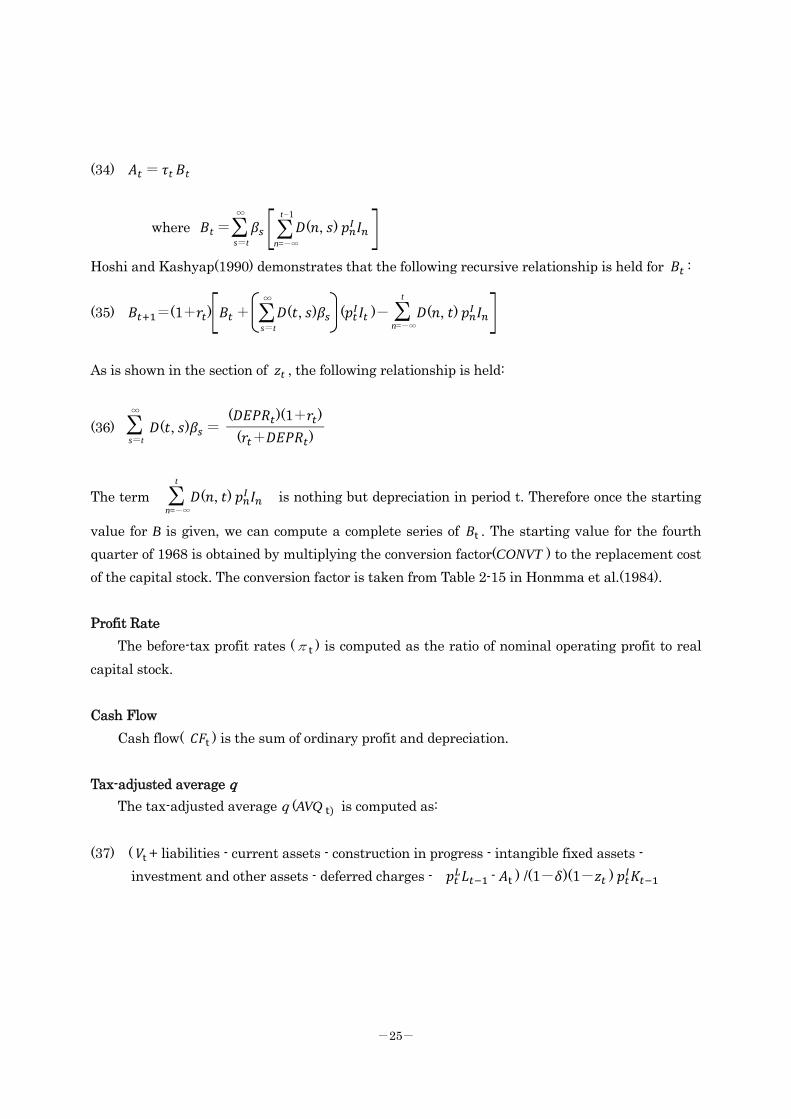
－25－

(34) ＝

where ＝ ( , )

Hoshi and Kashyap(1990) demonstrates that the following recursive relationship is held for :

(35) ＝(1＋ ) ＋ ( , ) ( )－ ( , )

As is shown in the section of , the following relationship is held:

(36) ( , ) ＝ ( )(1＋ )

( ＋ )

The term ( , ) is nothing but depreciation in period t. Therefore once the starting

value for B is given, we can compute a complete series of . The starting value for the fourth

quarter of 1968 is obtained by multiplying the conversion factor(CONVT ) to the replacement cost

of the capital stock. The conversion factor is taken from Table 2-15 in Honmma et al.(1984).

Profit Rate

The before-tax profit rates (π ) is computed as the ratio of nominal operating profit to real

capital stock.

Cash Flow

Cash flow( ) is the sum of ordinary profit and depreciation.

Tax-adjusted average q

The tax-adjusted average q (AVQ is computed as:

(37) ( + liabilities - current assets - construction in progress - intangible fixed assets -

investment and other assets - deferred charges - - ) /(1－ )(1－ )

∞

s＝t Σ

∞

s＝t Σ

∞

s＝t Σ

t－1

n=－∞ Σ

t

n=－∞ Σ

t

n=－∞ Σ

－26－

Footnotes

1) This naming of the current recession comes from the title of Miyazaki(1992) latest bestseller.

2) There is a growing body of literature on this issue. For example, see Greenwald and

Stiglitz(1988), Gertler and Hubbard(1988), and Bernanke and Gertler(1989) for theoretical

developments. For empirical pieces on the effects of internal net worth on investment, see Fazzari,

Hubbard, and Petersen(1988), Devereux and Schiantarelli(1990), Hubbard and Kashyap(1992),

and Whited( 1992).

3) Data on the SCOL, LCOL and SMALL variables come from Economic Statistics Annual, Bank of

Japan. That on TOPIX is from Annual Statistics on Tokyo Stock Exchange, Tokyo Stock Exchange

and the data of PLAND variable is taken from Land Price Index of Cities, Japan Real Estate

Institute.

4) Unfortunately the SMALL variable is not available over the whole sample period, since the

definition of small enterprises changed several times in the past. The consistent series is only

available since 1977.

5) Hayashi(1982) states the conditions that guarantee the equality of the average q with the

marginal q, present value of the marginal profitability from new investment divided by the price of

investment goods. They include perfect competition in the product market and the technology of

constant returns to scale.

6) The studies tackling this problem are now numerous. Bosworth(1975) asserts that the managers

will neglect what is going on in the stock market and follows the fundamentals. Fischer and

Merton(1984) asserts that as long as the value maximization of the current stockholders is the

principal objective of the corporations, then the managers will respect the market valuations in

making investment decisions. The empirical studies supporting the managers' obedience to the

stock market are Barro(1989) for the U.S. and Iwata(1990) and Takeda(1993) for Japan. Galeotti

and Schiantarelli(1990) and Blanchard, Rhee, and Summers(1990) show the evidence that the

fundamentals are as important as the non-fundamentals in the investment decision, but that the

response of investment to the fundamentals is larger than that to the non-fundamentals. Morck,

Shleifer, and Vishny(1990) gives the evidence that the stock prices exert a significant effect on

investment, but that the incremental explanatory power is only marginal.

－27－

7) We implicitly assume that the fundamentals are not so volatile as the stock price.

8) The industries covered in our sample are 16 industries in total. They are all industries,

agriculture, forestry and fishing, mining, construction, manufacturing, food and beverages, textiles,

pulp, paper and paper products, chemicals, steel, non-ferrous metals, fabricated metal products,

machinery, electrical machinery, wholesale and retail trade, and real estate. To save space we

report only five of them, all industries, construction, manufacturing, wholesale and retail trade, and

real estate. More detailed results on individual industry are available upon request.

9) An alternative approach is to treat land also as the physical capital which has different types of

adjustment costs. Under this specification, we can define the partial q for each physical capital, but

it is unobservable. For applications of this multiple q, see Wildasin(1984), Asako et al.(1989) and

Hayashi and Inoue(1991).

10) Derivation of tax-adjusted average q can be found in many studies analyzing the investment

behavior of the firm from the neoclassical viewpoint with adjustment costs. For example, see

Blundell et al.(1992).

11) Abel and Blanchard(1986) and Ohtaki and Suzuki(1986) construct the series of marginal q

based on the VAR model of underlying factors. Our approach is on the same track as them,

although we take univariate approaches rather than multivariate ones.

12) See Yamamoto(1988) for the ADF test and Perron(1988) for the Phillips-Perron test.

13) It is assumed here that the error terms do not have MA parts.

14) We assume that the firm forms the static expectations for the future tax rates.

15) The adjustment cost function is specified as a quadratic form:

( , ) ＝

－ ＋

－2

t 2 t

For more detailed derivation of eq.(14), see Blundell et al.(1992).

16) Inclusion of the market value of land in the investment function is justifiable when the

－28－

adjustment cost function is broadly defined so that it can incorporate the financial distress costs

and the value of land as a collateral works as a factor to mitigate the financial distress cost. Similar

formulation of the investment function is adopted by Devereux and Schiantarelli(1989) where an

inclusion of the variables such as cash flow and debt level is justified.

17) Seasonal dummies are also employed as regressors.

18) In a slightly different context Ueda and Yoshikawa(1986) demonstrate that average q cannot

be a sufficient statistics of investment. Noting that the profit rates have more permanent

components than the discount rates, they show that investment will be less responsive to financial

factors such as stock prices.

19) Pindyck(1990) stresses the irreversible nature of investment due to sunk costs. He points out

that investment becomes sensitive to the uncertainty with respect to future cash flow or interest

rates when irreversibility of investment is taken into consideration.

20) For example see Gertler and Hubbard(1988) and Bernanke and Gertler(1989).

21) Blanchard, Rhee, and Summers(1990) stresses this function of the stock market. They argue

that the corporation will issue a large volume of shares when the market overprices the corporation

and will invest the proceeds into the financial securities which do not require any additional cost in

adjusting its level. Our conjecture is that this is the case for Japan in the middle to the latter half of

80's. They also argue that in the case where the fundamentals differ from the market valuations the

reaction of the managers will hinge on what kind of shareholders the managers value most. If the

managers act for the interests of short-term shareholders, then they will respect the market

valuations, while if the managers side with the long-term shareholders, then they will act on the

basis of their perceived fundamentals. Judging from the mutual holdings of shares among the

corporations, it is likely that the latter will hold for Japan.

22) See pp.72-73 in Honmma et al.(1984).

23) See Table 2-13 of page 79 in Honmma et al.(1984).

24) For real estate industry land asset is defined broadly to include inventories

25) This market-book ratio is in between the case III and the case IV in Honmma et al.(1984). See

－29－

Table 2-7 of pp. 66-67 in Honmma et al.(1984).

26) Similar assumption is made in computing the land stock in Hoshi and Kashyap(1990).