Discrete Time Signal Processing Framework with Support Vector Machines

��0 Rojo-Álvarez, Martínez-Ramón, Camps-Valls, Martínez-Cruz, & Figuera

Copyright © 2007, Idea Group Inc. Copying or distributing in print or electronic forms without written permission of Idea Group Inc. is prohibited.

Chapter.VI

Discrete Time Signal Processing.Framework.with.

Support.Vector.MachinesJosé Luis Rojo-Álvarez, Universidad Rey Juan Carlos, Spain

Manel Martínez-Ramón, Universidad Carlos III de Madrid, Spain

Gustavo Camps-Valls, Universitat de València, Spain

Carlos E. Martínez-Cruz, Universidad Carlos III de Madrid, Spain

Carlos Figuera, Universidad Carlos III de Madrid, Spain

Abstract

Digital signal processing (DSP) of time series using SVM has been addressed in the litera-ture with a straightforward application of the SVM kernel regression, but the assumption of independently distributed samples in regression models is not fulfilled by a time-series prob-lem. Therefore, a new branch of SVM algorithms has to be developed for the advantageous application of SVM concepts when we process data with underlying time-series structure. In this chapter, we summarize our past, present, and future proposal for the SVM-DSP frame-work, which consists of several principles for creating linear and nonlinear SVM algorithms devoted to DSP problems. First, the statement of linear signal models in the primal problem

Discrete Time Signal Processing Framework with Support Vector Machines ���

Copyright © 2007, Idea Group Inc. Copying or distributing in print or electronic forms without written permission of Idea Group Inc. is prohibited.

(primal signal models) allows us to obtain robust estimators of the model coefficients in classical DSP problems. Next, nonlinear SVM-DSP algorithms can be addressed from two different approaches: (a) reproducing kernel Hilbert spaces (RKHS) signal models, which state the signal model equation in the feature space, and (b) dual signal models, which are based on the nonlinear regression of the time instants with appropriate Mercer’s kernels. This way, concepts like filtering, time interpolation, and convolution are considered and analyzed, and they open the field for future development on signal processing algorithms following this SVM-DSP framework.

Introduction

Support vector machines (SVMs) were originally conceived as efficient methods for pattern recognition and classification (Vapnik, 1995), and support vector regression (SVR) was sub-sequently proposed as the SVM implementation for regression and function approximation (e.g., Smola & Schölkopf, 2004). Many other digital signal processing (DSP) supervised and unsupervised schemes have also been stated from SVM principles, such as discriminant analysis (Baudat & Anouar, 2000), clustering (Ben-Hur, Hom, Siegelmann, & Vapnik, 2001), principal and independent component analysis (Bach & Jordan, 2002; Schölkopf, 1997), or mutual information extraction (Gretton, Herbrich, & Smola, 2003). Also, an interesting perspective for signal processing using SVM can be found in Mattera (2005), which relies on a different point of view of signal processing.The use of time series with supervised SVM algorithms has mainly focused on two DSP problems: (a) nonlinear system identification of the underlying relationship between two simultaneously recorded discrete-time processes, and (b) time-series prediction (Drezet & Harrison 1998; Gretton, Doucet, Herbrich, Rayner, & Schölkopf, 2001; Suykens, 2001). In both of them, the conventional SVR considers lagged and buffered samples of the available signals as its input vectors. Although good results in terms of signal-prediction accuracy are achieved with this approach, several concerns can be raised from a conceptual point of view. First, the basic assumption for the regression problem is that observations are independent and identically distributed; however, the requirement of independence among samples is not fulfilled at all by time-series data. Moreover, if we do not take into account the temporal dependence, we could be neglecting highly relevant structures, such as cor-relation or cross-correlation information. Second, most of the preceding DSP approaches use Vapnik’s e-insensitive cost function, which is a linear cost (that includes an insensitivity region). Nevertheless, when Gaussian noise is present in the data, a quadratic cost function should also be considered. Third, the previously mentioned methods take advantage of the well-known “kernel trick” (Aizerman, Braverman, & Rozoner, 1964) to develop nonlinear algorithms from a well-established linear signal processing technique. However, the SVM methodology has many other advantages, additional to the flexible use of Mercer’s kernels, which are still of great interest for many DSP problems that consider linear signal models. Finally, if we consider only SVR-based schemes, the analysis of an observed discrete-time sequence becomes limited because a wide variety of time-series structures are being ig-nored. Therefore, our purpose is to establish an appropriate framework for creating SVM algorithms in DSP problems involving time-series analysis. This framework is born from

��� Rojo-Álvarez, Martínez-Ramón, Camps-Valls, Martínez-Cruz, & Figuera

Copyright © 2007, Idea Group Inc. Copying or distributing in print or electronic forms without written permission of Idea Group Inc. is prohibited.

the consideration that discrete-time data should be treated in a conceptually different way from the SVR way in order to develop more advantageous applications of SVM concepts and performance to data with underlying time-series structure. In this chapter, we summa-rize our past, present, and future proposal for the SVM-DSP framework, which consists of creating SVM algorithms devoted to specific problems of DSP. A brief scheme of our proposal is presented in Figure 1. On the one hand, the statement of linear signal models in the primal problem, which will be called SVM primal signal models, will allow us to obtain robust estimators of the model coefficients (Rojo-Álvarez et al., 2005) in classical DSP problems, such as auto-regressive and moving-averaged (ARMA) model-ing, the g-filter, and the spectral analysis (Camps-Valls, Martínez-Ramón, Rojo-Álvarez, & Soria-Olivas, 2004; Rojo-Álvarez, Martínez-Ramón, Figueiras-Vidal, dePrado Cumplido, & Artés-Rodríguez, 2004; Rojo-Álvarez, Martínez-Ramón, Figueiras-Vidal, García-Armada, & Artés-Rodríguez, 2003). On the other hand, the consideration of nonlinear SVM-DSP algorithms can be addressed from two different approaches: (a) RKHS signal models, which state the signal model equation in the feature space (Martínez-Ramón, Rojo-Álvarez, Camps-Valls, Muñoz-Marí, Navia-Vázquez, Soria-Olivas, & Figueiras-Vidal, in press), and (b) dual signal models, which are based on the nonlinear regression of each single time instant with appropriate Mercer’s kernels (Rojo-Álvarez et al., 2006). While RKHS signal models allow us to scrutinize the statistical properties in the feature space, dual signal models yield an interesting and simple interpretation of the SVM algorithm under study in connection with the classical theory of linear systems.The rest of the chapter is organized as follows. In the next section, the e-Huber cost function (Mattera & Haykin, 1999; Rojo-Álvarez et al., 2003) is described, and the algorithm based on a generic primal signal model is introduced. SVM linear algorithms are then created for well-known time-series structures (spectral analysis, ARMA system identification, and the g-filter). An example of an algorithm statement from an RKHS signal model, the nonlinear ARMA system identification, is then presented. After that, SVM algorithms for time-series sinc interpolation and for nonblind deconvolution are obtained from dual signal models. A separate section presents simple application examples. Finally, some conclusions and several proposals for future work are considered.

Figure 1. Scheme of the proposal for a SVM-DSP framework described in this chapter. Our aim is to develop and create a variety of algorithms for time series processing that can benefit from the excellent properties of the SVM in a variety of different signal models.

Linear SVM-DSPalgorithms

Nonlinear SVM-DSPalgorithms

SVM-ARMA SVM-Spect SVM

Primal Signal Models

RKHS Signal Models

Dual Signal Models

SVM-ARMA

SVM-Sinc SVM-deconv SVM-Sinc SVM-deconv

SVM

Discrete Time Signal Processing Framework with Support Vector Machines ���

Copyright © 2007, Idea Group Inc. Copying or distributing in print or electronic forms without written permission of Idea Group Inc. is prohibited.

Primal.Signal. Models:.SVM.for.Linear.DSP

A first class of SVM-DSP algorithms are those obtained from primal signal models. Rather than the accurate prediction of the observed signal, the main estimation target of the SVM linear framework is a set of model coefficients or parameters that contain relevant informa-tion about the time-series data.In this setting, the use of the e-Huber cost function of the residuals allows us to deal with Gaussian noise in all the SVM-DSP algorithms, while still yielding robust estimations of the model coefficients. Taking into account that many derivation steps are similar when propos-ing different SVM algorithms, a general model is next included that highlights the common and the problem-specific steps of several preceding proposed algorithms (Rojo-Álvarez et al., 2005). Examples of the use of this general signal model for stating new SVM-DSP linear algorithms are given by creating an SVM algorithm version for the spectral analysis, the ARMA system identification, and the g-filter structure.

The e-Huber Cost As previously mentioned, the DSP of time series using SVM methodology has mainly fo-cused on two supervised problems (nonlinear time-series prediction and nonlinear system identification; Drezet & Harrison 1998; Gretton et al., 2001; Suykens, 2001), and both have been addressed from the straight application of the SVR algorithm. We start by not-ing that the conventional SVR minimizes the regularized Vapnik e-insensitive cost, which is in essence a linear cost. Hence, this is not the most suitable loss function in the presence of Gaussian noise, which will be a usual situation in time-series analysis. This fact was previously taken into account in the formulation of LS-SVM (Suykens, 2001), where a regularized quadratic cost is used for a variety of signal problems, but in this case, nonsparse solutions are obtained.

(a) (b) .

Figure 2. (a) In the e-Huber cost function, three different regions allow to adapt to differ-ent kinds of noise. (b) The nonlinear relationship between the residuals and the Lagrange multipliers provides with robust estimates of model coefficients.

��� Rojo-Álvarez, Martínez-Ramón, Camps-Valls, Martínez-Cruz, & Figuera

Copyright © 2007, Idea Group Inc. Copying or distributing in print or electronic forms without written permission of Idea Group Inc. is prohibited.

An alternative cost function of the residuals, the e-Huber cost, has been proposed (Mattera & Haykin, 1999; Rojo-Álvarez et al., 2003), which just combines both the quadratic and the e-insensitive cost functions. It has been shown to be a more appropriate residual cost, not only for time-series problems, but also for SVR in general (Camps-Valls, Bruzzone, Rojo-Álvarez, & Melgani, 2006). The e-Huber cost is represented in Figure 2a, and is given by:

2

2

0,1( ) ( ) ,

21( ) ,2

n

Hn n n C

n n C

e

L e e e e

C e C e e

≤

= − ≤ ≤ − − ≥

(1)

where en is the residual that corresponds to the nth observation for a given model, ce C= + ; e is the insensitive parameter, and δ and C control the trade-off between the regularization and the losses. The three different regions allow us to deal with different kinds of noise: the e-insensitive zone ignores absolute residuals lower than e; the quadratic cost zone uses the L2-norm of errors, which is appropriate for Gaussian noise; and the linear cost zone is an efficient limit for the impact of the outliers in the solution model coefficients. Note that equation (1) represents the Vapnik e-insensitive cost function when δ is small enough, the least squares (LS) cost function for C → ∞ and 0= , and the Huber cost function when 0= .

The Primal.Signal.Model

Let { }ny be a discrete-time series from which a set of N consecutive samples are measured and grouped into a vector of observations:

1 2[ , , , ]n Ny y y=y ' , (2) and let the set of vectors { }pz be a set of basis vectors spanning a P-dimensional subspace

PE of the N-dimensional Hilbert signal space NE . These vectors are described by:

1 2[ , , , ] , 1, ,p p p p

Nz z z p P= =z ' . (3)

Each observed signal vector y can be represented as a linear combination of elements of this basis set, plus an error vector 1[ , , ] 'Ne e=e modeling the measurement errors:

1

Pp p

pw

=

= +∑y z e. (4)

Discrete Time Signal Processing Framework with Support Vector Machines ���

Copyright © 2007, Idea Group Inc. Copying or distributing in print or electronic forms without written permission of Idea Group Inc. is prohibited.

For a given time instant n, a linear time-series model can be written as:

1

Pp p

n n n n np

y w z e e=

= + = +∑ w'v , (5)

where 1[ , , ]pw w=w ' is the model weight vector to be estimated, and 1[ , , ]pn n nz z=v '

represents the input space EI at time instant n. Equation (5) will be called the general pri-mal signal model, and it defines the time-series structure of the observations. This equation represents the functional relationship between the observations, the data (signals generating the projected signal subspace), and the model residuals. In practice, the general primal signal model equation is fulfilled by the n available observations. Note that input space EI is closely related to Hilbert signal subspace EP because the input vector at time instant n is given by the nth element of each of the basis space vectors of EP. For instance, in the case of a nonparametric spectral estimation, the basis of EP are the sinusoidal harmonics, whereas in the case of ARMA system identification, the basis of EP are the input signal and the delayed versions of input and output signals. The problem of estimating the coefficients can be stated as the minimization of:

2

1

1 ( )2

NH

nn

L e=

+ ∑w . (6)

Equivalently, by plugging equation (1) into equation (6), we have the following func-tional:

1 2 2

22 2 *2 *1 1 ( ) ( )

2 2 2n n n nn I n I n I

CC∈ ∈ ∈

+ + + + −∑ ∑ ∑w (7)

to be minimized with respect to w and ( ){ }n* , and constrained to

n n ny − ≤ +w'v (8)

*n n ny− + ≤ +w'v (9)

*, 0n n ≥ (10)

for n = 1, ..., N, where I1 and I2 are the observation indices whose residuals are in the qua-dratic and in the linear cost zone, respectively. The following expression for the coefficients is then obtained:

��� Rojo-Álvarez, Martínez-Ramón, Camps-Valls, Martínez-Cruz, & Figuera

Copyright © 2007, Idea Group Inc. Copying or distributing in print or electronic forms without written permission of Idea Group Inc. is prohibited.

1

Np p

n nn

w z=

= ∑ (11)

where n n n*= − .

Several properties of the method can be observed from these expressions.

1. Coefficient vector w can be expressed as a (possibly sparse) linear combination of input space vectors.

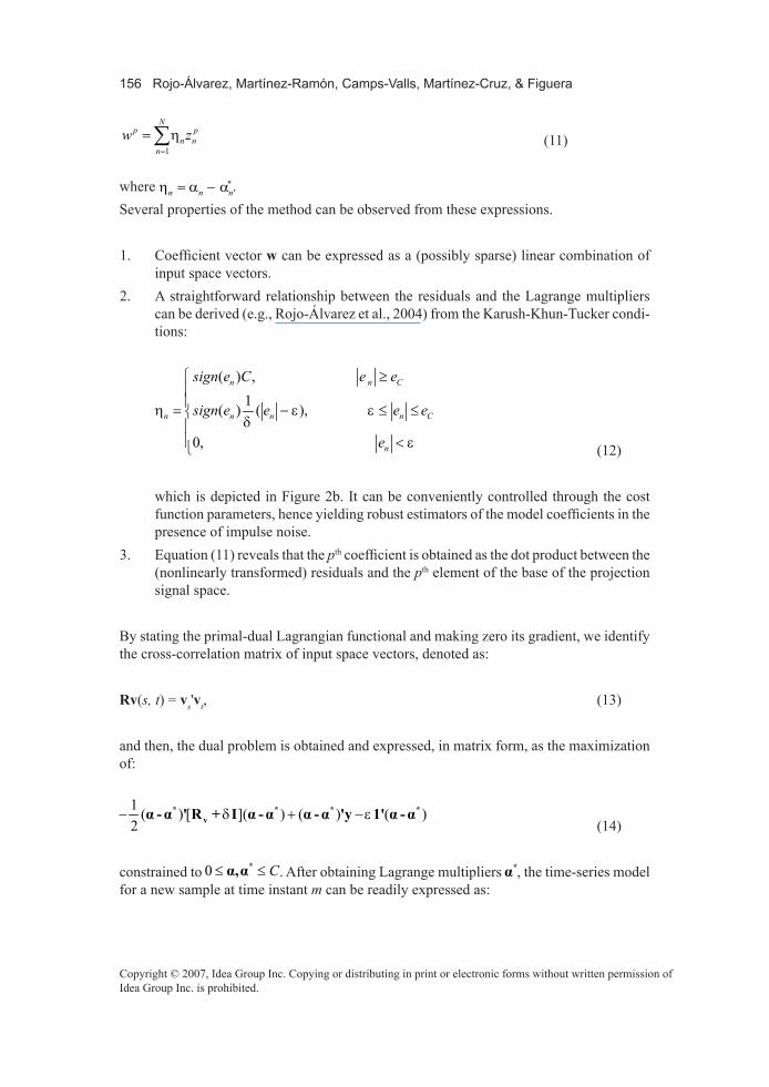
2. A straightforward relationship between the residuals and the Lagrange multipliers can be derived (e.g., Rojo-Álvarez et al., 2004) from the Karush-Khun-Tucker condi-tions:

( ) ,1( ) ( ),

0,

n n C

n n n n C

n

sign e C e e

sign e e e e

e

≥= − ≤ ≤ < (12)

which is depicted in Figure 2b. It can be conveniently controlled through the cost function parameters, hence yielding robust estimators of the model coefficients in the presence of impulse noise.

3. Equation (11) reveals that the pth coefficient is obtained as the dot product between the (nonlinearly transformed) residuals and the pth element of the base of the projection signal space.

By stating the primal-dual Lagrangian functional and making zero its gradient, we identify the cross-correlation matrix of input space vectors, denoted as:

Rv(s, t) = vs'vt, (13)

and then, the dual problem is obtained and expressed, in matrix form, as the maximization of:

1 ( ) [ ]( ) ( ) ( )2

− + −* * * *v (14)

constrained to 0 C≤ ≤* . After obtaining Lagrange multipliers *, the time-series model for a new sample at time instant m can be readily expressed as:

Discrete Time Signal Processing Framework with Support Vector Machines ���

Copyright © 2007, Idea Group Inc. Copying or distributing in print or electronic forms without written permission of Idea Group Inc. is prohibited.

1

ˆN

m n n mn

y=

= ∑ v 'v . (15)

Therefore, by taking into account the primal signal model in equation (5) that is used for a given DSP problem, we can determine signals p

nz that generate the Hilbert subspace where the observations are projected, and then the remaining elements and steps of the SVM methodology (such as the input space, the input space correlation matrix, the dual quadratic programming problem, and the solution) can be easily and immediately obtained. To illustrate this procedure, we next use this approach to propose three different linear SVM-DSP algorithms.

SVM.Spectral.Analysis

The SVM algorithm for spectral analysis (SVM-Spect; Rojo-Álvarez et al., 2003) can be stated as follows. Let { }

nty be a time series obtained by possibly nonuniformly sampling at

the corresponding time instants 1{ }Nt t, , of a continuous-time function ( )y t . A signal model using sinusoidal functions can be stated as:

1 1cos( ) (cos( ) sin( ))

n

N N

t i i n i n i i n i i n ni i

y A t e c t d t e= =

= + + = + +∑ ∑ , (16)

where the unknown parameters are amplitudes Ai, phases φi, and angular frequencies wi for a number Nw of sinusoidal components. The signals generating Hilbert subspace Ep are the discretized sinusoidal functions (phase and quadrature components), and hence, the model coefficients are obtained as:

1 1cos( ); sin( )

N N

l k l k l k l kk k

c t d t= =

= =∑ ∑ . (17)

The input space matrix correlation is given by the sum of two terms:

cos1

( , ) cos( ) cos( )N

i m i ki

R m k t t=

= ∑ (18)

and

sin1

( , ) sin( )sin( )N

i m i ki

R m k t t=

= ∑ , (19)

and the dual functional to be maximized is:

��� Rojo-Álvarez, Martínez-Ramón, Camps-Valls, Martínez-Cruz, & Figuera

Copyright © 2007, Idea Group Inc. Copying or distributing in print or electronic forms without written permission of Idea Group Inc. is prohibited.

cos sin1 ( ) [ ]( ) ( ) ( )2

− − + + − + − − +* * * * , (20)

constrained to 0 C≤ ≤* .

SVM-ARMA System Identification

The SVM algorithm for system identification basing on an explicit linear ARMA model1 was proposed in Rojo-Álvarez et al. (2004). Assuming that { }nx and { }ny are the input and the output, respectively, of a rational linear, time-invariant system, the corresponding dif-ference equation is:

11 1

QM

n i n i j n j ni j

y a y b x e− − += =

= + +∑ ∑ , (21)

where { }ia and { }jb are the M autoregressive and Q moving-averaged coefficients of the system, respectively. Here, the output signal in the present time lag is built as a weighted sum of the M-lag delayed versions of the same output signal, the input signal, and the Q-lag delayed versions of the input signal, and hence, these signals generate PE . The model coefficients are:

1

1 1

N N

i n n i j n n jn n

a y b x− − += =

= =∑ ∑ , (22)

and the input space correlation matrix is again the sum of two terms:

1( , )

M

m i k ii

m k y y− −=

= ∑MyR

(23)

and

1 11

( , )Q

m j k ij

m k x y− + − +=

= ∑QxR . (24)

These equations represent the time-local Mth and Qth order sample estimators of the values of the (non-Toeplitz) autocorrelation functions of the input and the output discrete-time processes, respectively. The dual problem consists of maximizing:

1 ( ) ( ) ( ) ( )2

− − + − + − − + * Q M * * *

x y , (25)

constrained to 0 C≤ ≤* .

Discrete Time Signal Processing Framework with Support Vector Machines ���

Copyright © 2007, Idea Group Inc. Copying or distributing in print or electronic forms without written permission of Idea Group Inc. is prohibited.

SVM g-Filter

The use of the primal signal model approach for stating an SVM version of the g-filter (Camps-Valls et al., 2004) is presented next. An important issue in time-series parametric modeling is how to ensure that the obtained model is causal and stable, which can be a requirement for AR time-series prediction and for ARMA system identification. A remark-able compromise between the stability and simplicity of adaptation can be provided by the g-filter, which was first proposed in Principe, deVries, and de Oliveira (1993). The g-filter can be regarded as a particular case of the generalized feed-forward filter, an infinite im-pulse response (IIR) digital filter with restricted feedback architecture. The g-structure, when used as a linear adaptive filter, results in a more parsimonious filter, and it has been used for echo cancellation (Palkar & Principe, 1994), time-series prediction (Kuo, Celebi, & Principe, 1994), system identification (Principe et al., 1999), and noise reduction (Kuo & Principe, 1994). Previous work on g-filters claims two main advantages: (a) It provides stable models, and (b) it permits the study of the memory depth of a model, that is, how much past information the model can retain. The g-filter is defined by using the difference equations of the linear ARMA model of a discrete-time series { }ny as a function of a given input sequence { }nx , as follows:

1

Pp p

n n np

y w x e=

= +∑ (26)

( ) 1

1 1

, 1

1 , 2, ,np

n p pn n

x px

x x p P−− −

== − + = , (27)

where m is a free parameter of the model. For m=1, the structure reduces to Widrow’s ada-line, whereas for 1≠ , it has an IIR transfer function due to the recursion in equation (27). The stability is trivially obtained with 0 1< < for a low-pass transfer function, and with

Figure 3. The gamma structure; the gamma filter can be seen as the cascade of IIR filters where loops are kept local and loop gain is constant

��0 Rojo-Álvarez, Martínez-Ramón, Camps-Valls, Martínez-Cruz, & Figuera

Copyright © 2007, Idea Group Inc. Copying or distributing in print or electronic forms without written permission of Idea Group Inc. is prohibited.

1 2< < for a high-pass transfer function. Figure 3 shows the g-filter structure corresponding to these equations. In comparison to general IIR filters, the feedback structure in the g-filter presents two complementary conditions: locality, since the loops are kept local with respect to the taps, and globality, since all the loops have the same loop gain 1-m. A proposed mea-surement of the memory depth of a model, which allows us to quantify the past information retained, is given by PM = , and it has units of time samples (Principe et al., 1993). For creating a linear SVM algorithmic version of the g-filter, we must identify the base of Hilbert signal subspace EP, which is just:

1 2[ , , , ] , 1,p p p pNx x x p P= =z '

, (28)

that is, the signals generating EP are the output signals after each g unit loop. Note that, for a previously fixed value of m, the generating signal vectors of the Hilbert projection space are straightforwardly determined. By denoting, as before, 1 , , P

n n nz z = v ' , the generic primal signal model in equation (5) can be used, the input space correlation matrix being given by equation (13), the dual problem by equation (14), and the output prediction model by equation (15). More details on the SVM g-filter can be found in Camps-Valls et al. (2004) and Rojo-Álvarez et al. (2005).

RKHS Signal Models: Nonlinear SVM-ARMA

Nonlinear SVM-DSP algorithms can be developed from two different general approaches, which are presented in this section and in the next one. Another class of SVM-DSP algo-rithms consists of stating the signal model of the time-series structure in the RKHS, and hence they will be called RKHS signal model based algorithms. The major interest of this approach is the combination of flexibility (provided by the nonlinearity to the algorithm) together with the possibility of scrutinizing the time-series structure of the model and the solution, despite the nonlinearity. In this section, the SVR algorithm for nonlinear system identification is briefly examined in order to check that, though efficient, this approach does not correspond explicitly to an ARMA model. Then, a nonlinear version of the linear SVM-ARMA algorithm is provided by using an explicit ARMA model on the RKHS. Nonlinear SVM-ARMA modeling is an example of the possibilities of the RKHS signal model approach for creating SVM-DSP algorithms, and the approach could be used with other DSP problems, for example, the g-filter, which is not discussed here (Camps-Valls, Requena-Carrión, Rojo-Álvarez, & Martínez-Ramón, 2006).

SVR System Identification

The SVR system identification algorithm (Gretton et al., 2001) can be described as follows. Let { }nx and { }ny be two discrete-time signals, which are the input and the output, respec-

Discrete Time Signal Processing Framework with Support Vector Machines ���

Copyright © 2007, Idea Group Inc. Copying or distributing in print or electronic forms without written permission of Idea Group Inc. is prohibited.

tively, of a nonlinear system. Let 1 1 2[ , , , ]n n n n My y y− − − −=y ' and 1 1[ , , , ]n n n n Qx x x− − +=x '

denote the states of input and output at discrete-time instant n. Assuming a nonlinear trans-formation φ([yn–1; xn]) for the concatenation of the input and output discrete-time processes to a B-dimensional feature space, : M QR F+ → , a linear regression model, can be built in F, and its equation is:

1([ ; ])n n n ny e−= +g' y x , (29)

where g = [g1, ..., gB]' is a vector of coefficients in the RKHS, and {en} are the residuals. By following the usual SVM methodology, the solution vector is:

11

([ ; ])N

n n nn

−=

= ∑g y x (30)

and the following Gram matrix containing the dot products can be identified:

1 1 1 1( , ) ( , ) ( , ) ([ ; ],[ ; ])m m k k m m k km k − − − −= =G y x ' y x y x y x , (31)

where the nonlinear mappings do not need to be explicitly calculated, but instead the dot product in RKHS can be replaced by Mercer’s kernels. The problem consists of maximizing the constrained functional:

[ ]1 ( ) ( ) ( ) ( )2

− + − + − − +* * * * . (32)

The predicted output for newly observed [ym–1; xm] is given by:

1 11

ˆ ([ , ],[ , ])N

m n n n m mn

y − −=

= ∑ y x y x . (33)

Note that equation (29) is the expression for a general nonlinear system identification model in the RKHS rather than an explicit ARMA structure. Moreover, though the reported perfor-mance of the algorithm is high when compared with other approaches, this formulation does not allow us to scrutinize the statistical properties of the time series that are being modeled in terms of autocorrelation and/or cross-correlation between the input and the output signals.

SVM-ARMA in RKHS

An explicit SVM-ARMA filter model can be stated in the RKHS by taking advantage of Mercer’s kernels’ properties. Assume that the state vectors of both the input and the output discrete-time signals can be separately mapped to two (possibly different) RKHSs by using a

��� Rojo-Álvarez, Martínez-Ramón, Camps-Valls, Martínez-Cruz, & Figuera

Copyright © 2007, Idea Group Inc. Copying or distributing in print or electronic forms without written permission of Idea Group Inc. is prohibited.

nonlinear mapping ( ) : Qx n xR F→x and 1( ) : M

y n yR F− →y . If a linear ARMA model is built in each of those RKHSs for the AR and for the MA model components, the corresponding difference equation is given by:

1( ) ( )n y n x n ny −= + +a' y b' x e , (34)

where 1, ,yBa a = a ' and 1, ,

xBb b = b ' are vectors determining the AR and the MA coefficients of the system, respectively, in the RKHSs, and By and Bx are the space dimen-sions.By writing down the primal problem, and then the primal-dual Lagrangian functional, the vector coefficients can be shown to be:

11 1

( ); ( )N N

n y n n x nn n

−= =

= =∑ ∑a y b x . (35)

We can identify two different kernel matrices: one for the input and another for the output vector, denoted and calculated as:

( ) ( ) ( ); 1 1 1 1,y m y m y k y m k− − − −= =R y ' y y y (36)

and

( ) ( ) ( ); ,x m x m x k x m k= =R x ' x x x . (37)

These equations account for the sample estimators of input and output time-series autocor-relation functions (Papoulis, 1991), respectively, in the RKHS space. Specifically, they are proportional to the non-Toeplitz estimator of each time-series autocorrelation matrix. The dual problem consists of maximizing, with the usual constraints, the functional:

1 ( ) [ ]( ) ( ) ( )2 x y− − + + − + − − +* * * * . (38)

The output for a new observation vector is obtained through:

1 11

ˆ ( ( , ) ( ))N

m n y n m x n mn

y − −=

= + +∑ y y x x . (39)

Note that this prediction model is different from equation (33), and for different real-data problems, we will be able to choose from one or another of the presented proposals.

Discrete Time Signal Processing Framework with Support Vector Machines ���

Copyright © 2007, Idea Group Inc. Copying or distributing in print or electronic forms without written permission of Idea Group Inc. is prohibited.

Dual.Signal.Models:................................Sinc. Interpolation.and.Deconvolution

An additional class of nonlinear SVM-DSP algorithms can be obtained by considering the nonlinear regression of the time lags or instants of the observed signals and using appropriate Mercer’s kernels. This class is known as the dual signal model based SVM algorithms. Here, we present this approach and pay attention to the interesting and simple interpretation of these SVM algorithms in connection with theory of linear systems. Although in dual signal models we use nonlinear kernels for their formulation, the resulting signal models are still linear (in the parameters) if we consider the final prediction equation. In this section, the statement of the sinc interpolation SVM algorithm is addressed follow-ing both a primal signal model and a dual signal model (Rojo-Álvarez et al., 2006). Given that the resulting dual signal model can be seen as the convolution of a sparse sequence (Lagrange multipliers) with the impulse response of a noncausal, linear, time-invariant system, given by the sinc kernel, the sinc model suggests the introduction of the SVM non-blind deconvolution algorithm, thus yielding a comparison between the resulting schemes for the primal and the dual signal models (Martínez-Cruz, Rojo-Álvarez, Camps-Valls, & Martínez-Ramón, 2006).

SVM.Sinc.Interpolation.

A classical DSP problem is the discrete time series interpolation with a noncausal sinc filter, which, in the absence of noise, gives the perfect reconstruction of uniformly sampled signals (Oppenheim & Schafer, 1989). However, the sinc reconstruction of a possibly nonuniformly sampled time series in the presence of noise is a hard problem to solve, and it has received special attention in the literature (Choi & Munson, 1995, 1998; Yen, 1956). The general problem can be stated as follows. Let x(t) be a band-limited, possibly Gaussian-noise-corrupted signal, and let { ( ) 1 }i ix x t i … N= , = , , be a set of N nonuniformly sampled observations. The sinc interpolation problem consists of finding an approximating function ˆ( )y t fitting the data, given by:

01

ˆ( ) ( ) ( ) sin ( ( )) ( )N

i ii

y t y t e t a c t t e t=

= + = − +∑ , (40)

where sin( )sinc( ) ttt = ,

00 T= is the bandwidth of the interpolating sinc units, and e(t) represents the noise. The previous continuous-time model, after nonuniform sampling, is expressed as the following discrete-time model:

01

ˆ( ) ( ) sinc( ( )) ( )N

j j j i j i ji

y y t e t a t t e t=

= + = − +∑ . (41)

An optimal band-limited interpolation algorithm, in the LS sense, was first proposed by Yen (1956). Given that we have as many free parameters as observations, this can become

��� Rojo-Álvarez, Martínez-Ramón, Camps-Valls, Martínez-Cruz, & Figuera

Copyright © 2007, Idea Group Inc. Copying or distributing in print or electronic forms without written permission of Idea Group Inc. is prohibited.

an ill-posed problem. In fact, in the presence of (even a low level of) noise, the coefficient estimations can often grow dramatically, leading to huge interpolation errors far away from the observed samples. To overcome this limitation, the regularization of the quadratic loss has also been proposed. The good properties of generalization and regularization of the SVM make it attractive to explore the possibility of creating SVM algorithms for sinc interpolation. From a primal signal model formulation, the signal model is equation (41), and the functions generating the projection signal subspace EP are the sinc functions centred at each sampling time instant,

0{ } {sinc( ( ))}pn n pz t t= − , for p = 1, ..., N. Therefore, the input space product matrix is:

0 01

( , ) sinc( ( ))sin ( ( ))N

n k n mn

k m t t c t t=

= − −∑T , (42)

And the primal coefficients { }ja are given by:

01

sinc( ( ))N

j i i ji

a t t=

= −∑ . (43)

The dual Lagrangian problem can now be stated as usual. A different SVM algorithm for sinc interpolation can be obtained by using the conventional SVR as follows. Given observations {yn} at time instants {tn}, we map the time instants to a feature space F by using nonlinear transformation φ, that is, : R F→ maps ( )t R t F∈ → ∈ . In the RKHS, a linear approximation to the transformed time instant can properly fit the observations:

ˆ ( )n ny t= w' (44)

for 1, ,n N= ; the weight vector in F is given by:

1( )

N

k j jj

t=

= ∑w . (45)

The following Gram matrix is identified:

( , ) ( ) ( ) ( , )k m k mk m t t t t= =G ' , (46)

where k(tk, tm) is a Mercer’s kernel, and, as usual, it allows one to obviate the explicit knowl-edge of nonlinear mapping ( )⋅ . The dual problem consists now of maximizing:

[ ]1 ( ) ( ) ( ) ( )2

− − + − + − − +* * * * , (47)

Discrete Time Signal Processing Framework with Support Vector Machines ���

Copyright © 2007, Idea Group Inc. Copying or distributing in print or electronic forms without written permission of Idea Group Inc. is prohibited.

constrained to ( )0 C*≤ ≤ . The final solution is expressed as:

1

ˆ ( , )N

m n n mn

y t t=

= ∑ . (48)

Moreover, we can define here k(tk, tn) = sinc(s(tk – tn)) as it is possible to show that it is a valid Mercer’s kernel (Zhang, Weida, & Jiao, 2004), called sinc Mercer’s kernel. Therefore, when using the sinc Mercer’s kernel, equation (48) can be seen as the nonuniform interpola-tion model given in equation (41). Note that other Mercer’s kernels could be easily used; for instance, if we define:

20

( , ) exp2k n

k n

t tt t

− = −

,

we obtain the Gaussian interpolator. Finally, we can observe that, for uniform sampling, equation (48) can be interpreted as the reconstruction of the observations given by a linear filter, where the impulse response of the filter is the sinc function, and the input signal is given by the sequence of the Lagrange multipliers corresponding to each time instant. That is, if we assume that {hn} are observa-tions from discrete-time process h[n], and that {k(tn)} are the samples of the discrete-time version of the sinc kernel, given by k[n], then solution ˆ[ ]y n can be written as a convolutional model given by:

ˆ[ ] [ ]* [ ]y n n n= , (49)

where * denotes the discrete-time convolution operator.Note that this expression is valid as far as we use an even Mercer’s kernel because in this case, the impulse response is symmetric. By allowing e to be nonzero, only a subset of the Lagrange multipliers will be nonzero, thus providing a sparse solution that is a highly desir-able property in the sinc interpolation problem.

SVM Nonblind Deconvolution

Another DSP problem that can be stated from an SVM approach is nonblind deconvolution. Given the observations of two discrete-time sequences { }ny and { }nh , we need to find the discrete-time sequence { }nx fulfilling:

*n n n ny x h e= + . (50)

��� Rojo-Álvarez, Martínez-Ramón, Camps-Valls, Martínez-Cruz, & Figuera

Copyright © 2007, Idea Group Inc. Copying or distributing in print or electronic forms without written permission of Idea Group Inc. is prohibited.

Similar to the SVM sinc interpolation case, we have two different approaches to this problem. The first one is a dual signal model approach, similar to the case of the SVM sinc interpola-tion. The solution of the nonlinear regression of the time instants is:

1

ˆ ( , )N

n i i ni

y t t=

= ∑ , (51)

and hence y[n] = h[n]* k[n]+e [n] is the convolutional model if we identify the Mercer’s kernel with the impulse response and the Lagrange multipliers with the input sequence to be estimated. This approach requires an impulse response being compatible with a Mercer’s kernel, for instance, being an autocorrelation sequence. However, in this case, one can obtain sparse solutions with an appropriate tuning of the free parameters. Another approach is the statement of the primal signal model, which is:

11

ˆN

n j n j nj

y x h e− +=

= +∑ . (52)

The signals generating the projection subspace are lagged versions of the impulse re-sponse:

1{ } { [ ]} { }pn n pz h n p h − += − = . (53)

The dual problem is the standard one, with the following correlation matrix:

1 11

( , )N

n k n mn

k m h h− + − +=

= ∑T . (54)

The main characteristics of the algorithm from the primal signal model are that the solution is, in general, nonsparse, and that any impulse response can be used (and not only Mercer’s kernels). Additionally, by noting that the solution can be expressed as:

1

1

ˆN

n i i ni

x h − +=

= ∑ , (55)

an implicit signal model can be seen, which is:

1ˆ * * *

N

k i i k k k Q k k k Qi Q

x h h h− + − + − +=

= = =∑ , (56)

where k Q+ denotes the samples of a Kronecker delta function that has been delayed Q samples, that is, the samples of discrete-time function [ ]k Q+ . Hence, the estimated signal is built

Discrete Time Signal Processing Framework with Support Vector Machines ���

Copyright © 2007, Idea Group Inc. Copying or distributing in print or electronic forms without written permission of Idea Group Inc. is prohibited.

as the convolution of the Lagrange multipliers with the time-reversed impulse response and with a Q-lag time-offset delta function. Figure 4 shows the schemes of both SVM algorithms. The residuals between the observa-tions and the model output are used to control the Lagrange multipliers. In the dual signal model based SVM algorithm, the Lagrange multipliers are the input to a linear, time-in-variant, noncausal system whose impulse response is the Mercer’s kernel. Interestingly, in the primal signal model based SVM algorithm, the Lagrange multipliers can be seen as the input to a single linear, time-invariant system whose global input response is heq[n] = h[n]* h[–n]*δ [n+Q]. It is easy to show that [ ]eqh n is the expression that corresponds (except for the delay) to a valid Mercer’s kernel, which emerges naturally from the primal dual model SVM formulation. This last point of view provides a new direction to explore the properties of the primal signal model SVM algorithms in connection with classical linear system theory, which is currently being studied. In particular, an intermediate method for providing sparse solutions while allowing us to use causal impulse responses in the model could benefit from the advantages of both kinds of approaches (Martínez-Cruz et al., 2006).

Some.Application.Examples

In this section, several examples are used to highlight the usefulness and capabilities of the SVM-DSP framework. An example of the SVM-Spect algorithm (Rojo-Álvarez et al., 2003) is used to show the insensitivity to impulse noise, using considerations that are also valid for the other schemes described in this chapter. Then, the properties of memory depth and regularization are studied for the SVM g-filter structure (Camps-Valls et al., 2004; Rojo-Álvarez et al., 2005). The application of SVR and the described SVM-ARMA algorithms in a nonlinear system estimation is included, as presented in Martínez-Ramón et al. (in press). Finally, an example using SVM sinc in nonuniform interpolation is summarized (Rojo-Álvarez et al., 2005).

Figure 4. Algorithms for nonblind deconvolution. Schemes of the primal signal model (left) and for the dual signal model (right).

��� Rojo-Álvarez, Martínez-Ramón, Camps-Valls, Martínez-Cruz, & Figuera

Copyright © 2007, Idea Group Inc. Copying or distributing in print or electronic forms without written permission of Idea Group Inc. is prohibited.

SVM-Spect.and.Insensitivity.to.Outliers.

A simple synthetic data example is first presented to show the capacity of SVM-Spect to deal with outliers. A discrete-time process is given by:

( )sin 2n n ny fn v j= + + , (57)

where f = 0.3; vn is a white, Gaussian-noise sequence with zero mean and variance s2 = 0.1; and jn is an impulsive noise process, generated as a sparse sequence for which 30% of the samples, randomly placed, are high-amplitude values given by 10 ( 0 5 0 5)U± + − . , . , where ()U denotes the uniform distribution in the given interval, and the remaining are null samples. The number of observed samples is N =128, and we set 2 64N N= / = (Figure 5a). A pre-vious simulation showed that 0= was a proper choice. A low value of δ leads to a major

Figure 5. Insensitivity of SVM-Spect to impulse noise. (a) Sinusoid whithin impulsive noise (up) and its Welch periodogram (down). (b) Histogram of the residuals (scaled to δ= 10) and control of the outlier impact onto the solution with C. (c) SVM-Spect spectral estimators for different values of insensitivity, which is controlled by the product δC.

Discrete Time Signal Processing Framework with Support Vector Machines ���

Copyright © 2007, Idea Group Inc. Copying or distributing in print or electronic forms without written permission of Idea Group Inc. is prohibited.

emphasis on minimizing the losses so that overfitting to the observations occurs in this case. We select a moderately high value of 10= . The appropriate a priori choice of free parameter C can be addressed by considering that, according to equation (22) the solution coefficients are a function of the multipliers and the data. Also, equations (12) and (13) reveal that a high amplitude residual, corresponding to an outlier, will produce a high amplitude multiplier, which will distort the solution. However, if the maximum value that the multiplier can take is properly limited by C, the impact of the outlier on the solution is lessened. Figure 5b shows that C should be low enough to exclude the residual amplitudes greater than the base level. This level can be obtained from previous methods of estimation of the prediction error, from a priori knowledge of the problem, or from training data. Figure 5c shows the results for 2 1 2C = , . , and 0.2, the last one allow-ing us to recover the spectral peak. Other experiments, not included here, show that similar solutions are obtained for a range of values of C being low enough.

Figure 6. Performance criterion for the identification of an elliptic filter by the LS g-filter (thin) and the SVM g-filter (thick) for different orders (P between 1 and 4). The optimal m parameter is also indicated for all the methods.

��0 Rojo-Álvarez, Martínez-Ramón, Camps-Valls, Martínez-Cruz, & Figuera

Copyright © 2007, Idea Group Inc. Copying or distributing in print or electronic forms without written permission of Idea Group Inc. is prohibited.

Example.with.SVM g-Filter

The performance of the SVM g-filter is examined next in terms of memory depth and regularization. In this experiment, we focused on the main advantages of both the g-filter structure (stability and memory depth) and the SVM (regularization). We compared the memory parameter m in the LS, the SVM, and the regularized g-filters. The last one used the leaky LS algorithm described in Harris, Juan, and Principe (1999), which was introduced to alleviate the stalling of the filter coefficients in a real-time hardware implementation. We identified the following third-order elliptic low-pass filter:

( )1 2 3

1 2 3

0.0563 0.0009 0.0009 0.05631 2.129 1.7834 0.5435

z z zH zz z z

− − −

− − −

− + +=

− + +, (58)

which was previously analyzed in Principe et al. (1993) because of its long impulse response. A 100-sample input discrete process { }nx is a white, Gaussian-noise sequence with zero mean and unit variance. The corresponding output signal { }ny was corrupted by additive, small-variance ( 2 0 1e = . ), random processes, modeling the measurement errors. An independent set of 100 samples was used for testing, and the experiment was repeated 100 times. Figure 6 shows the chosen performance criterion ( ) ( )min n nJ var e var y= / (Principe et al., 1993) as a function of m and P in the test set. It is noteworthy that, in all cases, the adaline structure (m =1) performs worse than the g structures. In addition, the SVM g-filter clearly improves the results of the LS and the regularized versions in terms of minJ . The memory depth M for a fixed P increases with lower values of m. This trend (observed for the three methods) is especially significant for the regularized g-filter, but it occurs at the expense of poor performance of the criterion. Nevertheless, the SVM g-filter still presents a good trade-off between memory depth and performance.

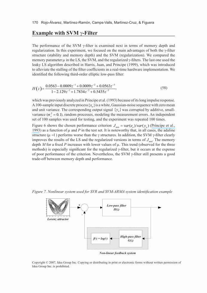
Figure 7. Nonlinear system used for SVR and SVM-ARMA system identification example

Low-pass filterH(z)

High-pass filterG(z)

+

-

f(·) = log(·)

-20 -15 -10 -5 0 5 10 15 205

10

15

20

25

30

35

40

45

x

Lorenz attractor

Non-linear feedback system

Discrete Time Signal Processing Framework with Support Vector Machines ���

Copyright © 2007, Idea Group Inc. Copying or distributing in print or electronic forms without written permission of Idea Group Inc. is prohibited.

SVR and SVM-ARMA Non-Linear System Identification

We will now compare the performance in nonlinear system identification of SVR to the SVM-ARMA formulation provided in the chapter. We used the RBF kernel, which gives universal nonlinear mapping capabilities, and because only one kernel free parameter has to be tuned.For illustration purposes, we run an example with explicit input-output relationships. The system that generated the data is illustrated in detail in Figure 7. The input discrete-time signal to the system is generated using a Lorenz system, which is described by the solution of the following three simultaneous differential equations:

/dx dt x y= − + , (59)

/dy dt xz rx y= − + − (60)

/dz dt xy bz= − , (61)

with 10= , 28r = , and 8 3b = / . The chaotic nature of the time series is made explicit by plotting a projection of the trajectory in the x−z plane. Only the x component was used as an input signal to the system, and thus the model must perform the more difficult task of state estimation. This signal was then passed through an eighth-order low-pass finite impulse response (FIR) filter, H(z), with cutoff frequency 0 5n = . and normalized gain of -6dB at

n. The output signal was then passed through a feedback loop consisting of a high-pass minimum-phase channel:

( ) 1 2 3

11.00 2.01 1.46 0.39

G zz z z− − −=

+ + +, (62)

and further distorted with the nonlinearity ( ) ( )f log⋅ = ⋅ . The resulting system performs an extremely complex operation, in which the relationship between the input and output signals has an important effect in the time-series dynamics. The described system was used to generate 1,000 input and output samples, which were split into two sets: a cross-validation data set to select the optimal free parameter consisting of 50 samples, and a test set to assess model performance, containing the following 500 samples. In all experiments, we selected the model order, s, C, e, and δ by following the usual cross-

Table 1. Mean error (ME), mean-squared error (MSE), mean absolute error (ABSE), correla-tion (r), and normalized MSE (with respect of variance), for the models at the test set.

Eq. ME MSE ABSE r nMSE

SVR (33) 0.28 3.07 1.08 0.99 -0.82

SVM-ARMA (39) 0.14 2.08 0.88 0.99 -0.92

��� Rojo-Álvarez, Martínez-Ramón, Camps-Valls, Martínez-Cruz, & Figuera

Copyright © 2007, Idea Group Inc. Copying or distributing in print or electronic forms without written permission of Idea Group Inc. is prohibited.

Figure 8. SVM sinc interpolation from primal and dual signal models.(a) Training, test, and reconstructed signals in the time domain. (b) Training, test, and reconstructed signals in the spectral domain. (c) Spectral representation of the test signal and of the optimum kernel after validation.

(a)

(b)

Discrete Time Signal Processing Framework with Support Vector Machines ���

Copyright © 2007, Idea Group Inc. Copying or distributing in print or electronic forms without written permission of Idea Group Inc. is prohibited.

Figure 8. Continued

(c)

validation method. The experiment was repeated 100 times with randomly selected starting points in the time series. Averaged results are shown in Table 1, where it can be seen a general reduction in several merit figures for SVM-ARMA system identification.

SVM.Sinc.Interpolation.

In order to see the basic features of the primal and dual signal model SVM algorithms for sinc interpolation, the recovery of a signal with relatively lower power energy on high frequency was addressed. This signal was chosen to explore the potential effect that regularization could have on the high-frequency components. The observed signals consisted of the sum of two squared sincs, one of them being a lower level, amplitude-modulated version of the baseband component, thus producing the following band-limited signal:

( ) 2

0

1sinc ( )(1 sin(2 )) ( )2

y t t ft e tT

= + + , (63)

where f = 0.4 Hz. A set of L =32 samples was used with averaged sampling interval T = 0.5s. Sampling intervals falling outside [0, LT] were wrapped inside. The sampling instants were uniform. The signal-to-noise ratio was 10dB. The performance of the interpolators was

��� Rojo-Álvarez, Martínez-Ramón, Camps-Valls, Martínez-Cruz, & Figuera

Copyright © 2007, Idea Group Inc. Copying or distributing in print or electronic forms without written permission of Idea Group Inc. is prohibited.

Figure 9. SVM sinc interpolation. (a) Temporal representation of the Lagrange multipliers. (b) Spectral representation of the Lagrange multipliers. Primal: Lagrange multipliers for SVM-P; primal coefs: coefficients for SVM-P; dual: Lagrange multipliers for SVM-D; RBF: Lagrange multipliers for SVM-R.

(a)

measured by building a test set consisting of a noise-free, uniformly sampled version of the output signal with sampling interval T/16 as an approximation of the continuous-time signal, and by comparing it with the predicted interpolator outputs at the same time instants. Figure 8 represents the resulting training and test signals, in the temporal (a) and in the spectral (b) domains, together with the results of the interpolation of the primal and dual signal model with the sinc kernel (SVM-P and SVM-D, respectively), the dual signal model with the RBF kernel (SVM-R), and the regularized Yen algorithm (Y2). Figure 8c shows that the spectral bandwidth of the optimum kernels after validation matched closely to the test signal bandwidth. As can be seen in Figure 9b, the spectral shape of the Lagrange multipliers always clearly provides the spectral shape of the test signal, either very similar to the sinc kernel, or compensating for the fading spectral shape of the RBF kernel. The time representation of the Lagrange multipliers (Figure 9a) shows that the coefficients and the Lagrange multipliers in the primal dual model and the Lagrange multipliers in the dual signal model are very similar (though not exactly the same), but the sparseness obtained by the RBF kernel is higher than that obtained by the sinc kernel.

Discrete Time Signal Processing Framework with Support Vector Machines ���

Copyright © 2007, Idea Group Inc. Copying or distributing in print or electronic forms without written permission of Idea Group Inc. is prohibited.

Future.Directions

This chapter has summarized the SVM-DSP framework, which pursuits to exploit the SVM properties in signal processing problems by taking into account the temporal structure of the data to be modeled. To our understanding, this approach opens several research directions, and our aim here has been just to summarize the wide variety of methods that emerge when simple properties, such as the model equation, are considered. A more formalized statement of these concepts should be elaborated. An interesting research direction for the SVM-DSP framework is the use of complex arithmetic, which opens the fields of both digital com-munications and array processing to the possibilities of SVM methodology. These topics are analyzed in Chapters VII and VIII.There are many other topics that will deserve special attention, some of them being the following:

Figure 9. Continued

(b)

��� Rojo-Álvarez, Martínez-Ramón, Camps-Valls, Martínez-Cruz, & Figuera

Copyright © 2007, Idea Group Inc. Copying or distributing in print or electronic forms without written permission of Idea Group Inc. is prohibited.

• Free-parameter.selection: The choice of the free parameters of both the e-Huber cost and the used kernel is not always a trivial task, and a theoretical and practical analy-sis of the resampling techniques used to date (e.g., k-fold and bootstrap resampling) should be addressed. Additionally, the Bayesian point of view using the regularized expectation-maximization (EM) algorithm could be explored. The temporal structure of the DSP problems should be taken into account in this setting.

• Computational.burden: Due to the use of quadratic programming and to the need for free-parameter selection, the computational burden required by these algorithms can preclude its use to online signal processing applications and to adaptive versions.

• The choice of an appropriate kernel: For nonlinear models, the SVM in general requires the choice of an appropriate Mercer’s kernel among a variety of available known ones. A systematic procedure for determining which kernel is appropriate for a given real problem would be desirable.

• Detailed.comparison.for.each.algorithm: Our presentation does not address the detailed comparison of SVM-DSP algorithms to advanced methods, but this is a topic to consider in each new SVM algorithm.

Acknowledgments

Portions reprinted, with permission, from Rojo-Álvarez et al. (2004) and Rojo-Álvarez et al. (2003; © 2006 IEEE). Portions reprinted, with permission, from Rojo-Álvarez et al. (2005; © 2006 Elsevier). C. E. Martínez-Cruz is partially supported by Alban (EU Programme of High Level Scholarships for Latin America) scholarship No. E04M037994SV.

References

Aizerman, A., Braverman, E. M., & Rozoner, L. I. (1964). Theoretical foundations of the potential function method in pattern recognition learning. Automation and Remote Control, 25, 821-837.

Bach, F. R., & Jordan, M. I. (2002). Kernel independent component analysis. Journal of Machine Learning Research, 3, 1-48.

Baudat, G., & Anouar, F. (2000). Generalized discriminant analysis using a kernel approach. Neural Computation, 12(2), 2385-2404.

Ben-Hur, A., Horn, D., Siegelmann, H., & Vapnik, V. (2001). Support vector clustering. Journal of Machine Learning Research, 2, 125-137.

Camps-Valls, G., Bruzzone, L., Rojo-Álvarez, J. L., & Melgani, F. (2006). Robust support vector regression for biophysical parameter estimation from remotely sensed images. IEEE Geoscience and Remote Sensing Letters, 3(3), 339-343.

Discrete Time Signal Processing Framework with Support Vector Machines ���

Copyright © 2007, Idea Group Inc. Copying or distributing in print or electronic forms without written permission of Idea Group Inc. is prohibited.

Camps-Valls, G., Martínez-Ramón, M., Rojo-Álvarez, J. L., & Soria-Olivas, E. (2004). Robust gamma-filter using support vector machines. Neurocomputing, 62, 493-499.

Camps-Valls, G., Requena-Carrión, J., Rojo-Álvarez, J. L., & Martínez-Ramón, M. (2006). Nonlinear gamma-filter using support vector machines (Tech. Rep. No. TR-DIE-TSC-22/07/2006). Spain: University of Valencia & University Carlos III of Madrid.

Choi, H., & Munson, D. C., Jr. (1995). Analysis and design of minimax-optimal interpolators. In Proceedings of IEEE International Conference on Acoustics, Speech, and Signal Processing ( ICASSP’95) (Vol. 2, pp. 885-888).

Choi, H., & Munson, D. C., Jr. (1998). Analysis and design of minimax-optimal interpola-tors. IEEE Transactions on Signal Processing, 46(6), 1571-1579.

Drezet, P., & Harrison, R. (1998). Support vector machines for system identification. UKACC International Conference on Control’98 (Vol. 1, pp. 688-692).

Gretton, A., Doucet, A., Herbrich, R., Rayner, P., & Schölkopf, B. (2001). Support vector regression for black-box system identification. 11th IEEE Workshop on Statistical Signal Processing (pp. 341-344).

Gretton, A., Herbrich, R., & Smola, A. (2003). The kernel mutual information. In Proceedings of the IEEE International Conference on Acoustics, Speech, and Signal Processing (ICASSP’03) (Vol. 4, pp. 880-883).

Harris, J. G., Juan, J.-K., & Principe, J. C. (1999). Analog hardware implementation of continuous-time adaptive filter structures. Journal of Analog Integrated Circuits and Signal Processing, 18(2), 209-227.

Kuo, J. M., Celebi, S., & Principe, J. (1994). Adaptation of memory depth in the gamma filter. In Proceedings of IEEE International Conference on Acoustics, Speech, and Signal Processing (ICASSP94) (Vol. 5, pp. 373-376).

Kuo, J. M., & Principe, J. (1994). Noise reduction in state space using the focused gamma model. In Proceedings of IEEE International Conference on Acoustics, Speech, and Signal Processing (ICASSP94) (Vol. 2, pp. 533-536).

Martínez-Cruz, C. E., Rojo-Álvarez, J. L., Martínez-Ramón, M., Camps-Valls, G., Muñoz-Marí, J., & Figueiras-Vidal, A. R. (2006). Sparse deconvolution using support vector machines (Tech. Rep. No. TR-DIE-TSC-10/09/2006). Spain: University Carlos III of Madrid & University of Valencia.

Martínez-Ramón, M., Rojo-Álvarez, J., Camps-Valls, G., Muñoz-Marí, J., Navia-Vázquez, A., Soria-Olivas, E., & Figueiras-Vidal, A.R. (in press). Support vector machines for non-linear kernel arma system identification. IEEE Transactions on Neural Networks.

Mattera, D. (2005). Support vector machines for signal processing. In L. Wang (Ed.), Sup-port vector machines: Theory and applications (pp. 321-342). Springer.

Mattera, D., & Haykin, S. (1999). Support vector machines for dynamic reconstruction of chaotic systems. In B. Schölkopf, C. Burges, & A. Smola (Eds.), Advances in kernel methods (pp. 211-242). MIT Press.

Oppenheim, A., & Schafer, R. (1989). Discrete-time signal processing. Englewood Cliffs, NJ: Prentice Hall.

��� Rojo-Álvarez, Martínez-Ramón, Camps-Valls, Martínez-Cruz, & Figuera

Copyright © 2007, Idea Group Inc. Copying or distributing in print or electronic forms without written permission of Idea Group Inc. is prohibited.

Palkar, M., & Principe, J. (1994). Echo cancellation with the gamma filter. In Proceed-ings of IEEE International Conference on Acoustics, Speech and Signal Processing (ICASSP94) (Vol. 3, pp. 369-372).

Papoulis, A. (1991). Probability random variables and stochastic processes (3rd ed.). New York: McGraw-Hill.

Principe, J. C., deVries, B., & de Oliveira, P. G. (1993). The gamma filter: A new class of adaptive IIR filters with restricted feedback. IEEE Transactions on Signal Process-ing, 41(2), 649-656.

Reed, M., & Simon, B. (1980). Functional analysis. London: Academic Press. Rojo-Álvarez, J. L., Camps-Valls, G., Martínez-Ramón, M., Soria-Olivas, E., Navia Vázquez,

A., & Figueiras-Vidal, A. R. (2005). Support vector machines framework for linear signal processing. Signal Processing, 85(12), 2316-2326.

Rojo-Álvarez, J.L., Figuera, C., Martínez-Cruz, C., Camps-Valls, G., & Martínez-Ramón, M. (2006). Sinc kernel nonuniform interpolation of time series with support vector machines (Tech. Rep. No. TR-DIE-TSC-01/07/2006). Spain: University Carlos III of Madrid & University of Valencia.

Rojo-Álvarez, J.L., Martínez-Ramón, M., Figueiras-Vidal, A. R., dePrado Cumplido, M., & Artés-Rodríguez, A. (2004). Support vector method for ARMA system identification. IEEE Transactions on Signal Processing, 52(1), 155-164.

Rojo-Álvarez, J. L., Martínez-Ramón, M., Figueiras-Vidal, A. R., García-Armada, A., & Artés-Rodríguez, A. (2003). A robust support vector algorithm for non-parametric spectral analysis. IEEE Signal Processing Letters, 10(11), 320-323.

Schölkopf, B. (1997). Support vector learning. Munich, Germany: R. Oldenbourg Verlag. Smola, A. J., & Schölkopf, B. (2004). A tutorial on support vector regression. Statistics and

Computing, 14(3), 199-222. Suykens, J. (2001). Support vector machines: A nonlinear modelling and control perspective.

European Journal of Control, 7(2-3), 311-327. Vapnik, V. (1995). The nature of statistical learning theory. New York: Springer. Yen, J. L. (1956). On nonuniform sampling of bandwidth-limited signals. IRE Transactions

on Circuit Theory, CT-3, 251-257. Zhang, L., Weida, Z., & Jiao, L. (2004). Wavelet support vector machine. IEEE Transactions

on System, Man and Cybernetics B, 34(1), 34-39.

Endnote

1 The notation of ARMA is used according to the consideration of an ARMA filter structure, however, from a system identification point of view, the model is an ARX (exogenous).