Discrete signals - University of Pennsylvania

Discrete signals

Alejandro RibeiroDept. of Electrical and Systems Engineering

University of [email protected]

http://www.seas.upenn.edu/users/~aribeiro/

January 18, 2017

Signal and Information Processing Discrete signals 1

mailto:[email protected]

http://www.seas.upenn.edu/users/~aribeiro/

Discrete signals

Discrete signals

Inner products and energy

Discrete complex exponentials


Discrete signals

I Discrete and finite time index n = 0, 1, . . . ,N − 1 = [0,N − 1].

I Discrete signal x is a function mapping [0,N − 1] to a real value x(n)

x : [0,N − 1]→ R

I The values that the signal takes at time index n is x(n)

I Sometimes it will make sense to talk about complex signals

x : [0,N − 1]→ C

I The values x(t) = xR(t) + j xI (t) are complex numbers

I Space of signals = space of N-dimensional vectors RN or CN


Deltas (impulses, spikes)

I The discrete delta function δ(n) is a spike at (initial) time n = 0

δ(n) =

{1 if n = 00 else

0 1 2 3 4 5 6 70

0.5

1

Time index n = 0, 1, . . . , 7 = [0, 7]

Sig

na

lx

(n)

Delta function x(n) = δ(n)

I The shifted delta function δ(n − n0) has a spike at time n = n0

δ(n−n0) =

{1 if n = n0

0 else0 1 2 3 4 5 6 7

0

0.5

1

Time index n = 0, 1, . . . , 7 = [0, 7]

Sig

na

lx

(n)

Shifted delta function x(n) = δ(n − 3)

I This is not a new definition, just a time shift


Constants and square pulses

I A constant function x(n) has the same value c for all n

x(n) = c , for all n

0 2 4 6 8 10 12 140

0.5

1

Time index n = 0, 1, . . . , 15 = [0, 15]

Sig

na

lx

(n)

Constant function x(n) = 1

I A square pulse of width M, uM(n), equals one for the first M values

uM(n) =

{1 if 0 ≤ n < M0 if M ≤ n

0 2 4 6 8 10 12 140

0.5

1

Time index n = 0, 1, . . . , 15 = [0, 15]

Sig

na

lx

(n)

Square pulse x(n) = u6(n)

I Can consider shifted pulses uM(n − n0), with n0 < N −M


Units: Sampling time and signal duration

I Sampling time Ts ⇒ Time elapsed between indexes n and n + 1

⇒ Sampling frequency fs := 1/Ts

I Time index n represents actual time t = nTs

0 0.25 0.5 0.75 1 1.25 1.5 1.750

0.5

1

Time t (in seconds)

Sig

na

lx

(t)

Square pulse of duration 1s observed during 2s at a sampling rate Ts = 125ms

I Signal duration T = NTs ⇒ Time length of signal

⇒ The last sample is “held” during Ts time units


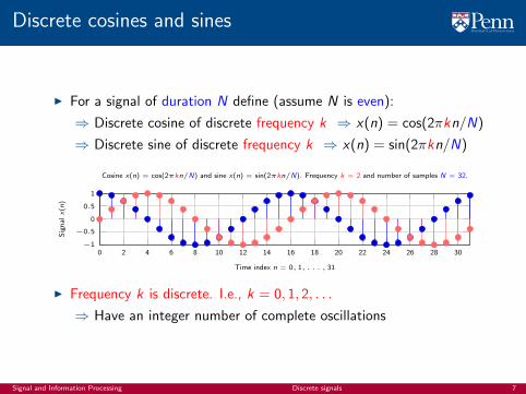
Discrete cosines and sines

I For a signal of duration N define (assume N is even):

⇒ Discrete cosine of discrete frequency k ⇒ x(n) = cos(2πkn/N)

⇒ Discrete sine of discrete frequency k ⇒ x(n) = sin(2πkn/N)

0 2 4 6 8 10 12 14 16 18 20 22 24 26 28 30−1

−0.5

0

0.5

1

Time index n = 0, 1, . . . , 31

Sig

na

lx

(n)

Cosine x(n) = cos(2πkn/N) and sine x(n) = sin(2πkn/N). Frequency k = 2 and number of samples N = 32.

I Frequency k is discrete. I.e., k = 0, 1, 2, . . .

⇒ Have an integer number of complete oscillations


Cosines of different frequencies (1 of 2)

I Discrete frequency k = 0 is a constant

I Discrete frequency k = 1 is a complete oscillation

I Frequency k = 2 is two oscillations, for k = 3 three oscillations ...

0 2 4 6 8 10 12 14 16 18 20 22 24 26 28 30−1

−0.5

0

0.5

1

Frequency k = 0. Number of samples N = 32

0 2 4 6 8 10 12 14 16 18 20 22 24 26 28 30−1

−0.5

0

0.5

1


0 2 4 6 8 10 12 14 16 18 20 22 24 26 28 30−1

−0.5

0

0.5

1


0 2 4 6 8 10 12 14 16 18 20 22 24 26 28 30−1

−0.5

0

0.5

1



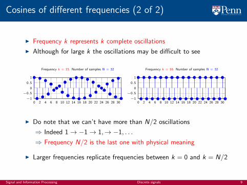
Cosines of different frequencies (2 of 2)

I Frequency k represents k complete oscillations

I Although for large k the oscillations may be difficult to see

0 2 4 6 8 10 12 14 16 18 20 22 24 26 28 30−1

−0.5

0

0.5

1


0 2 4 6 8 10 12 14 16 18 20 22 24 26 28 30−1

−0.5

0

0.5

1


I Do note that we can’t have more than N/2 oscillations

⇒ Indeed 1→ −1→ 1,→ −1, . . .

⇒ Frequency N/2 is the last one with physical meaning

I Larger frequencies replicate frequencies between k = 0 and k = N/2


Duplicated frequencies

I Frequencies k and N − k represent the same cosine

0 2 4 6 8 10 12 14 16 18 20 22 24 26 28 30−1

−0.5

0

0.5

1


0 2 4 6 8 10 12 14 16 18 20 22 24 26 28 30−1

−0.5

0

0.5

1

Frequency N − k = 31. Number of samples N = 32

0 2 4 6 8 10 12 14 16 18 20 22 24 26 28 30−1

−0.5

0

0.5

1


0 2 4 6 8 10 12 14 16 18 20 22 24 26 28 30−1

−0.5

0

0.5

1

Frequency N − k = 30. Number of samples N = 32

I Actually, if k + l = N, cosines of frequencies k and l are equivalent

I Not true for sines, but almost. The signals have opposite signs


Discrete frequencies and actual frequencies

I What is the discrete frequency k of a cosine of frequency f0?

I Depends on sampling time Ts , frequency fs = 1Ts

, duration T = NTs

I Period of discrete cosine of frequency k is T/k (k oscillations)

I Thus, regular frequency of said cosine is ⇒ f0 =k

T=

k

NTs=

k

Nfs

I A cosine of frequency f0 has discrete frequency k = (f0/fs)N

I Only frequencies up to N/2↔ fs/2 have physical meaning

I Sampling frequency fs ⇒ Cosines up to frequency f0 = fs/2


Use of units example

I Generate N = 32 samples of an A note with sampling frequency fs = 1, 760Hz

I The frequency of an A note is f0 = 440Hz. This entails a discrete frequency

k =f0fsN =

440Hz

1, 760Hz32 = 8

0 2 4 6 8 10 12 14 16 18−1

−0.5

0

0.5

1

Time t (in miliseconds)

Sig

na

lx

(t)

The A note observed during T = NTs = 18.2ms with a sampling rate fs = 1, 760Hz

I Alternatively ⇒ x(n) = cos[2πkn/N

]= cos

[2π(f0/fs)Nn/N

]I Which simplifies to ⇒ x(n) = cos

[2π(f0/fs)n

]= cos

[2πf0(nTs)

]Signal and Information Processing Discrete signals 12

Noninteger frequencies

I The frequency k need not be integer but it’s not a discrete cosine

⇒ Sampled cosine ⇒ x(n) = cos(2πkn/N)

⇒ Sampled sine ⇒ x(n) = sin(2πkn/N)

I Discrete sine and cosine have complete oscillations

I Sampled sine and cosine may have incomplete oscillations

I Discrete sine and cosine are used to define Fourier transforms (later)



Discrete signals




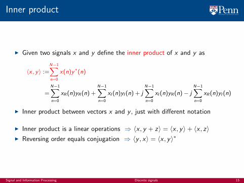
Inner product

I Given two signals x and y define the inner product of x and y as

〈x , y〉 :=N−1∑n=0

x(n)y∗(n)

=N−1∑n=0

xR(n)yR(n) +N−1∑n=0

xI (n)yI (n) + jN−1∑n=0

xI (n)yR(n)− jN−1∑n=0

xR(n)yI (n)

I Inner product between vectors x and y , just with different notation

I Inner product is a linear operations ⇒ 〈x , y + z〉 = 〈x , y〉+ 〈x , z〉I Reversing order equals conjugation ⇒ 〈y , x〉 = 〈x , y〉∗


Inner product interpretation

I Signal inner product has same intuition as vector inner product

⇒ Inner product 〈x , y〉 is the projection of y on x

⇒ The value of 〈x , y〉 is how much of y falls in x direction

I E.g., if 〈x , y〉 = 0 the signals are orthogonal. They are “unrelated”

xy

〈x , y〉 > 0

x

y

〈x , y〉 > 0

x

y

〈x , y〉 = 0

x

y

〈x , y〉 < 0

xy

〈x , y〉 < 0


Norm and energy

I Following the algebra analogies, define the norm of signal x as

‖x‖ :=

[ N−1∑n=0

|x(n)|2]1/2

=

[ N−1∑n=0

|xR(n)|2 +N−1∑n=0

|xI (n)|2]1/2

I More important, define the energy of the signal as the norm squared

‖x‖2 :=N−1∑n=0

|x(n)|2 =N−1∑n=0

|xR(n)|2 +N−1∑n=0

|xI (n)|2

I For complex numbers x(n)x∗(n) = |xR(n)|2 + |xI (n)|2 = |x(n)|2

I Thus, we can write the energy as ⇒ ‖x‖2 = 〈x , x〉


Cauchy Schwarz inequality

I The largest an inner product can be is when the vectors are collinear

−‖x‖ ‖y‖ ≤ 〈x , y〉 ≤ ‖x‖ ‖y‖

I Or in terms of energy ⇒ 〈x , y〉2 ≤ ‖x‖2 ‖y‖2

I If you are the sort of person that prefers explicit expressions

N−1∑n=0

x(n)y∗(n) ≤[ N−1∑

n=0

|x(n)|2][ N−1∑

n=0

|y(n)|2]

I The equalities hold if and only if x and y are collinear


Example: Square pulse of unit energy

I The unit energy square pulse is the signal uM(n) that takes values

uM (n) =1√M

if 0 ≤ n < M

uM (n) = 0 if M ≤ nt

uM (n)

1/√M

M − 1 N − 1

I To compute energy of the pulse we just evaluate the definition

‖ uM ‖2 :=N−1∑n=0

| uM (n)|2 =M−1∑n=0

∣∣∣(1/√M)∣∣∣2 =

M

M= 1

I Indeed, the unit energy square pulse has unit energy

I If the height of the pulse is 1 instead of 1/√M, the energy is M.


Shifted pulses

I To shift a pulse we modify the argument ⇒ uM(n − K )

⇒ The pulse is now centered at K (n = K is as n = 0 before)

t

uM (n)

1/√M

M − 1 K K + M − 1 N − 1

I Inner product of two pulses with disjoint support (K ≥ M)

〈uM(n),uM(n − K )〉 :=N−1∑n=0

uM(n) uM (n − K ) = 0

I The signals are orthogonal, and indeed, “unrelated” to each other


Overlapping shifted pulses

I Inner product of two pulses with overlapping support (K < M)

〈uM(n),uM(n − K)〉 :=N−1∑n=0

uM(n) uM (n − K)

I The signals overlap between K and M − 1. Thus

〈uM(n),uM(n − K)〉 =M−1∑n=K

(1/√M)(

1/√M)

=M − K

M= 1− K

M

t

uM (n)

1/√M

K M − 1 K + M − 1 N − 1

I Inner product is proportional to the relative overlap

⇒ which is, indeed, how much the signals are “related” to each other



Discrete signals




Discrete Complex exponentials

I Discrete complex exponential of discrete frequency k and duration N

ekN(n) =1√N

e j2πkn/N =1√N

exp(j2πkn/N)

I The complex exponential is explicitly given by

e j2πkn/N = cos(2πkn/N) + j sin(2πkn/N)

I Real part is a discrete cosine and imaginary part a discrete sine

0 2 4 6 8 10 12 14 16 18 20 22 24 26 28 30−1

−0.5

0

0.5

1

Re(ej2πkn/N

), with k = 2 and N = 32

0 2 4 6 8 10 12 14 16 18 20 22 24 26 28 30−1

−0.5

0

0.5

1

Im(ej2πkn/N

), with k = 2 and N = 32


Properties

[P1] For frequency k = 0, the exponential ekN(n) = e0N(n) is a constant

ekN(n) =1√N

=1√N

1

[P2] For frequency k = N, the exponential ekN(n) = eNN(n) is a constant

eNN(n) =e j2πNn/N

√N

=(e j2π)n√

N=

(1)n√N

=1√N

I Actually, true for any frequency k ∈ N (multiple of N)

[P3] For k = N/2, the exponential ekN(n) = eN/2N(n) = (−1)n/√N

eN/2N(n) =e j2π(N/2)n/N

√N

=(e jπ)n√

N=

(−1)n√N

I The fastest possible oscillation with N samples

That e j2π = 1 follows from e jπ = −1, which follows from e jπ + 1 = 0. The latter

relates the five most important constants in mathematics and proves god’s existence.


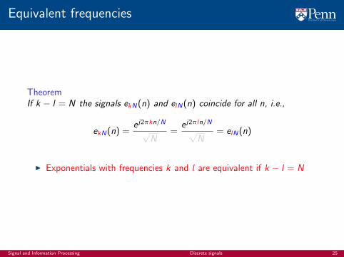
Equivalent frequencies

TheoremIf k − l = N the signals ekN(n) and elN(n) coincide for all n, i.e.,

ekN(n) =e j2πkn/N√

N=

e j2πln/N√N

= elN(n)

I Exponentials with frequencies k and l are equivalent if k − l = N


Proof of equivalence

Proof.

I We prove by showing that ekN(n)/elN(n) = 1. Indeed,

ekN(n)

elN(n)=

e j2πkn/N

e j2πln/N= e j2π(k−l)n/N

I But since we have that k − l = N the above simplifies to

ekN(n)

elN(n)= e j2πNn/N =

[e j2π

]n= 1n = 1


Canonical frequency sets

ARI

I Exponentials with frequencies that are N apart are equivalent

−N, −N + 1, . . . , −10, 1, . . . , N − 1N, N + 1, . . . , 2N − 1

I Suffice to look at N consecutive frequencies, e.g., k = 0, 1, . . .N − 1

I Another canonical choice is to make k = 0 the center frequency

−N/2 + 1, . . . , −1, 0, . . . , N/2N/2 + 1, . . . , N − 1, N, . . . , 3N/2

I With N even (as usual) use N/2 positive and N/2− 1 negative

I From one canonical set to the other ⇒ Chop and shift


Orthogonality

TheoremComplex exponentials with nonequivalent frequencies are orthogonal. I.e.

〈ekN , elN〉 = 0

when k − l < N. E.g., when k = 0, . . .N − 1, or k = −N/2 + 1, . . . ,N/2.

I Signals of canonical sets are “unrelated.” Different rates of change

I Also note that the energy is ‖ekN‖2 = 〈ekN , ekN〉 = 1

I Exponentials with frequencies k = 0, 1, . . . ,N − 1 are orthonormal

〈ekN , elN〉 = δ(l − k)

I They are an orthonormal basis of signal space with N samples


Proof of orthogonality

Proof.

I Use definitions of inner product and discrete complex exponential to write

〈ekN , elN〉 =N−1∑n=0

ekN(n)e∗lN(n) =N−1∑n=0

e j2πkn/N√N

e−j2πln/N

√N

I Regroup terms to write as geometric series

〈ekN , elN〉 =1

N

N−1∑n=0

e j2π(k−l)n/N =1

N

N−1∑n=0

[e j2π(k−l)/N

]nI Geometric series with basis a sums to

∑N−1n=0 an = (1− aN)/(1− a). Thus,

〈ekN , elN〉 =1

N

1−[e j2π(k−l)/N

]N1− e j2π(k−l)/N

=1

N

1− 1

1− e j2π(k−l)/N= 0

I Completed proof by noting[e j2π(k−l)/N

]N= e j2π(k−l) =

[e j2π

](k−l)

= 1


Conjugate frequencies

TheoremOpposite frequencies k and −k yield conjugate signals: e−kN = e∗kN(n)

Proof.

I Just use the definitions to write the chain of equalities

e−kN(n) =e j2π(−k)n/N

√N

=e−j2πkn/N√

N=

[e j2πkn/N√

N

]∗= e∗kN(n)

I Opposite frequencies ⇒ Same real part. Opposite imaginary part

⇒ The cosine is the same, the sine changes sign


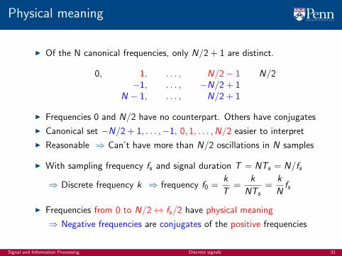
Physical meaning

I Of the N canonical frequencies, only N/2 + 1 are distinct.

0, 1, . . . , N/2− 1 N/2−1, . . . , −N/2 + 1

N − 1, . . . , N/2 + 1

I Frequencies 0 and N/2 have no counterpart. Others have conjugates

I Canonical set −N/2 + 1, . . . ,−1, 0, 1, . . . ,N/2 easier to interpret

I Reasonable ⇒ Can’t have more than N/2 oscillations in N samples

I With sampling frequency fs and signal duration T = NTs = N/fs

⇒ Discrete frequency k ⇒ frequency f0 =k

T=

k

NTs=

k

Nfs

I Frequencies from 0 to N/2↔ fs/2 have physical meaning

⇒ Negative frequencies are conjugates of the positive frequencies


Complex exponentials for N = 2 and N = 4

I When N = 2 only k = 0 and k = 1 represent distinct signals

0 1−1−0.5

00.5

1

k = −2 (k = 0)

0 1−1−0.5

00.5

1

k = −1 (k = 0)

0 1−1−0.5

00.5

1

k = 0

0 1−1−0.5

00.5

1

k = 1

0 1−1−0.5

00.5

1

k = 2 (k = 0)

0 1−1−0.5

00.5

1

k = 3 (k = 1)

I The signals are real, they have no imaginary parts

I When N = 4, k = 0, 1, 2 are distinct. k = −1 is conjugate of k = 1

0 1 2 3−1−0.5

00.5

1

k = −2 (k = 2)

0 1 2 3−1−0.5

00.5

1

k = −1

0 1 2 3−1−0.5

00.5

1

k = 0

0 1 2 3−1−0.5

00.5

1

k = 1

0 1 2 3−1−0.5

00.5

1

k = 2

0 1 2 3−1−0.5

00.5

1

k = 3 (k = −1)

I Can also use k = 3 as canonical instead of k = −1 (conjugate of k = 1)


Complex exponentials for N = 8

I Frequencies from k = 1 to k = 4 represent distinct signals

0 1 2 3 4 5 6 7−1

−0.5

0

0.5

1

k = 0

0 1 2 3 4 5 6 7−1

−0.5

0

0.5

1

k = 1

0 1 2 3 4 5 6 7−1

−0.5

0

0.5

1

k = 2

0 1 2 3 4 5 6 7−1

−0.5

0

0.5

1

k = 3

0 1 2 3 4 5 6 7−1

−0.5

0

0.5

1

k = 4

I Frequencies k = −1 to k = −3 are conjugate signals of k = 1 to k = 3

0 1 2 3 4 5 6 7−1

−0.5

0

0.5

1

k = −1

0 1 2 3 4 5 6 7−1

−0.5

0

0.5

1

k = −2

0 1 2 3 4 5 6 7−1

−0.5

0

0.5

1

k = −3

I All other frequencies represent one of the signals above


Complex exponentials for N = 16

I There are 9 distinct frequencies and 7 conjugates (not shown). Some look likeactual oscillations. Border effect of k = 0 and k = N/2 becomes less relevant

0 2 4 6 8 10 12 14−1

−0.5

0

0.5

1

k = 0

0 2 4 6 8 10 12 14−1

−0.5

0

0.5

1

k = 1

0 2 4 6 8 10 12 14−1

−0.5

0

0.5

1

k = 2

0 2 4 6 8 10 12 14−1

−0.5

0

0.5

1

k = 3

0 2 4 6 8 10 12 14−1

−0.5

0

0.5

1

k = 4

0 2 4 6 8 10 12 14−1

−0.5

0

0.5

1

k = 5

0 2 4 6 8 10 12 14−1

−0.5

0

0.5

1

k = 6

0 2 4 6 8 10 12 14−1

−0.5

0

0.5

1

k = 7

0 2 4 6 8 10 12 14−1

−0.5

0

0.5

1

k = 8


Discrete signals - University of Pennsylvania

Documents