Modélisation discrète de la régulation du métabolisme énergétique des cellules eukaryotes et validation formelle de sa dynamique Rajeev KHOODEERAM Laboratoire d’Informatique, de Signaux et Systèmes de Sophia Antipolis (I3S) UMR7271 Université Côte d’Azur CNRS Présentée en vue de l’obtention du grade de docteur en Informatique d’Université Côte d’Azur Dirigée par : Gilles BERNOT, Professeur, Université Côte d’Azur Co-encadrée par : Jean-Yves TROSSET, Re- sponsable Projets Bio & Chimie Informatique, Sup’ BioTech, Paris Soutenue le : 8 Novembre 2021 Devant le jury, composé de : Gilles BERNOT, Professeur, Université Côte d’Azur Jean-Yves TROSSET, Responsable Projets, Sup’ BioTech, Paris Olivier ROUX, Professeur, Ecole Centrale de Nantes Marie BEURTON-AIMAR, HDR, Maître de Con- férences, Université Bordeaux 1 Pascale LE GALL, Professeur, École Centrale de Paris Vidushi S. NEERGHEEN, Professeur associé, Uni- versité de Maurice

Welcome message from author
This document is posted to help you gain knowledge. Please leave a comment to let me know what you think about it! Share it to your friends and learn new things together.
Transcript
Modélisation discrète de la régulation du métabolismeénergétique des cellules eukaryotes et validation formelle de
sa dynamique
Rajeev KHOODEERAM
Laboratoire d’Informatique, de Signaux et Systèmes de Sophia Antipolis (I3S)UMR7271 Université Côte d’Azur CNRS
Présentée en vue de l’obtentiondu grade de docteur en Informatiqued’Université Côte d’Azur
Dirigée par : Gilles BERNOT, Professeur,Université Côte d’AzurCo-encadrée par : Jean-Yves TROSSET, Re-sponsable Projets Bio & Chimie Informatique, Sup’BioTech, Paris
Soutenue le : 8 Novembre 2021
Devant le jury, composé de :Gilles BERNOT, Professeur, Université Côte d’AzurJean-Yves TROSSET, Responsable Projets, Sup’BioTech, ParisOlivier ROUX, Professeur, Ecole Centrale de NantesMarie BEURTON-AIMAR, HDR, Maître de Con-férences, Université Bordeaux 1Pascale LE GALL, Professeur, École Centrale deParisVidushi S. NEERGHEEN, Professeur associé, Uni-versité de Maurice

Discrete modelling of the energy metabolism regulation of eukaryotic cellsand formal validation of its dynamics
Modélisation discrète de la régulation du métabolisme énergétique descellules eukaryotes et validation formelle de sa dynamique
Rajeev KHOODEERAM
Président du jury : Pascale LE GALL, Professeur, École Centrale de Paris.
Rapporteurs
Olivier ROUX, Professeur, École Centrale de Nantes
Marie BEURTON-AIMAR, HDR, Maître de Conférences, Université Bordeaux 1
Examinateurs
Pascale LE GALL, Professeur, École Centrale de Paris.
Vidushi S. NEERGHEEN, Professeur associé, Université de Maurice
Directeur de thèse
Gilles BERNOT, Professeur, Université Côte D’azur
Co-Encadrant de thèse
Jean-Yves TROSSET, Responsable Projets Bio & Chimie Informatique, Sup’ BioTech, Paris

Discrete modelling of the energy metabolism regulation of eukaryotic cells and formalvalidation of its dynamics
Abstract
We present a formal model of the regulation of the energetic metabolism in eukaryotic cells. The mainoriginality of this model is to consider explicitly an abstraction of the main metabolic processes that pilotthis metabolism, thereby greatly reducing the number of variables in the model. Moreover, the mod-elling framework proposed by Réné Thomas is particularly well suited for a qualitative view of regulatorynetworks resulting in a model with 14 variables and 112 parameters, with integer values. However, themodel contains a lot of feedback loops which are intricately linked and which makes the dynamic of thesystem very complex. As in all complex system modelling, the main difficulty is to identify the value ofall parameters in a coherent way with respect to known dynamic behaviours.
The identification of parameters has been smoothed due to a large repertoire of knowledge in molec-ular biology, and the validation of the proposed model has been done by model checking, in more than160 temporal logic formulas (including the main metabolic phenotypes, notably the Warburg effect). Ithas been a meticulate process which has been successful by putting in place a solid and pluridisciplinarymethod of modelling together with a software platform (DyMBioNet), both pivotal for this thesis. Themodel has been conceived to be used as a backbone, which can be plugged with other regulatory net-works like the cell cycle or the circadian clock, for potential applications to cancer or chronotherapy.The DyMBioNet software is bundled with three main functionalities including verifying system proper-ties with CTL, simulation as well as visualisation of a complex system. Furthermore, this well-definedmethodology, and its software platform DyMBioNet, would be useful to directly construct other formalregulatory networks of large size.
Keywords: Modelling, Biological networks, Formal logics, Metabolism
Modélisation discrète de la régulation du métabolisme énergétique des cellules eukary-otes et validation formelle de sa dynamique
Résumé
Nous présentons une modélisation formelle de la régulation du métabolisme énergétique de la celluleeucaryote. Le choix original de cette modélisation est de considérer explicitement des abstractions desprincipaux processus cellulaires qui pilotent ce métabolisme, réduisant ainsi considérablement le nombrede variables à prendre en compte dans le modèle. De plus, le formalisme de modélisation introduit parRéné Thomas est particulièrement adapté à une vision qualitative des phénomènes de régulation, desorte que le modèle repose sur seulement 14 variables et 112 paramètres entiers. En revanche, le modèlepossède de nombreux cycles de retroaction fortement intriqués, qui rendent la dynamique du système trèscomplexe. Comme dans toute modèlisation de système complexe, la difficulté majeure est l’identificationdes valeurs des paramètres de manière cohérente avec les comportements dynamiques connus.
L’identification des paramètres a été effectuée sur la base d’une abondante connaissance biologiquemoléculaire, et la validation du modèle a été effectuée par model checking sur plus de 160 formulestemporelles (incluant les principaux phénotypes connus, en particulier l’effet Warburg). Il s’agit d’untravail minutieux qui n’a pu être mené à son terme qu’en mettant en place une méthode pluridisciplinairede modélisation et une plateforme logicielle (DyMBioNet), qui constituent également une contributionimportante de la thèse. Le modèle achévé a été conçu comme un "noyau formel" réutilisable en connexionavec d’autres réseaux de régulation comme le cycle cellulaire et l’horloge circadienne, par exemple en vued’application au cancer ou à la chronothéraphie. L’outil DyMBioNet présente plusieurs fonctionnalitésincluant la possibilité de faire des preuves en CTL, la simulation ainsi que la visualisation d’un systèmecomplexe. Enfin, la méthodologie définie ici et son outillage DyMBioNet pourront être réutilisés directe-ment pour construire d’autres modèles formels de régulation de grande taille.
Mots-clés: Modélisation, Réseaux biologiques, Logique formelles, Métabolisme


Dedications
To my parents, for giving me the most powerful tool in my life,Education
To my wife and kids, for bearing with me, and for being my source ofmotivations
To my supervisors, always there for helping and guiding me
To my University, for providing me all forms of support
To all those people, who have always underestimated me
To God, for this beautiful life on Earth !

Contents
1 INTRODUCTION 11.1 Abstract view of metabolism . . . . . . . . . . . . . . . . . . . . . . . . . . . . . . . . . . 11.2 Choice of formalism . . . . . . . . . . . . . . . . . . . . . . . . . . . . . . . . . . . . . . . 21.3 An indispensable methodology . . . . . . . . . . . . . . . . . . . . . . . . . . . . . . . . . 21.4 DyMBioNet platform . . . . . . . . . . . . . . . . . . . . . . . . . . . . . . . . . . . . . . . 31.5 Thesis roadmap . . . . . . . . . . . . . . . . . . . . . . . . . . . . . . . . . . . . . . . . . . 4
2 REGULATION OF THE CELL ENERGY METABOLISM 62.1 Introduction . . . . . . . . . . . . . . . . . . . . . . . . . . . . . . . . . . . . . . . . . . . . 62.2 Catabolism . . . . . . . . . . . . . . . . . . . . . . . . . . . . . . . . . . . . . . . . . . . . 7
2.2.1 Nutrients . . . . . . . . . . . . . . . . . . . . . . . . . . . . . . . . . . . . . . . . . 72.2.1.1 Dual view of nutrients . . . . . . . . . . . . . . . . . . . . . . . . . . . . . 72.2.1.2 Sugar, lipids and amino acids (glutamine) as carbon sources . . . . . . . 72.2.1.3 Glutamine as a major nitrogen and carbon sources . . . . . . . . . . . . . 82.2.1.4 Other nutrients . . . . . . . . . . . . . . . . . . . . . . . . . . . . . . . . 8
2.2.2 Glycolysis . . . . . . . . . . . . . . . . . . . . . . . . . . . . . . . . . . . . . . . . . 82.2.2.1 A global view . . . . . . . . . . . . . . . . . . . . . . . . . . . . . . . . . . 82.2.2.2 ATP production . . . . . . . . . . . . . . . . . . . . . . . . . . . . . . . . 102.2.2.3 A building block synthetic pathway: PPP . . . . . . . . . . . . . . . . . . 10
2.2.3 Fermentation . . . . . . . . . . . . . . . . . . . . . . . . . . . . . . . . . . . . . . . 112.2.4 Respiration . . . . . . . . . . . . . . . . . . . . . . . . . . . . . . . . . . . . . . . . 11
2.2.4.1 Oxidative Krebs . . . . . . . . . . . . . . . . . . . . . . . . . . . . . . . . 122.2.4.2 Reductive Krebs . . . . . . . . . . . . . . . . . . . . . . . . . . . . . . . . 132.2.4.3 Oxidative phosphorylation . . . . . . . . . . . . . . . . . . . . . . . . . . 13
2.2.5 Energy yields . . . . . . . . . . . . . . . . . . . . . . . . . . . . . . . . . . . . . . . 142.2.6 Alternative Catabolic Pathways . . . . . . . . . . . . . . . . . . . . . . . . . . . . . 15
2.3 Anabolism: from energy to biomass . . . . . . . . . . . . . . . . . . . . . . . . . . . . . . . 152.3.1 Introduction . . . . . . . . . . . . . . . . . . . . . . . . . . . . . . . . . . . . . . . 152.3.2 Protein synthesis . . . . . . . . . . . . . . . . . . . . . . . . . . . . . . . . . . . . . 162.3.3 Lipid synthesis . . . . . . . . . . . . . . . . . . . . . . . . . . . . . . . . . . . . . . 16
2.4 Regulation of metabolism . . . . . . . . . . . . . . . . . . . . . . . . . . . . . . . . . . . . 172.4.1 Metabolic oscillations . . . . . . . . . . . . . . . . . . . . . . . . . . . . . . . . . . 172.4.2 Metabolic shuttles . . . . . . . . . . . . . . . . . . . . . . . . . . . . . . . . . . . . 17
2.5 Conclusion of the chapter . . . . . . . . . . . . . . . . . . . . . . . . . . . . . . . . . . . . 18
3 FRAMEWORKS FOR THE DYNAMICS OF BIOLOGICAL NETWORKS 203.1 Introduction . . . . . . . . . . . . . . . . . . . . . . . . . . . . . . . . . . . . . . . . . . . . 203.2 Classical frameworks for metabolism . . . . . . . . . . . . . . . . . . . . . . . . . . . . . . 21
3.2.1 General concepts . . . . . . . . . . . . . . . . . . . . . . . . . . . . . . . . . . . . . 213.2.2 Flux Balance Analysis . . . . . . . . . . . . . . . . . . . . . . . . . . . . . . . . . . 243.2.3 Elementary Flux Modes . . . . . . . . . . . . . . . . . . . . . . . . . . . . . . . . . 263.2.4 Conclusion on metabolic frameworks . . . . . . . . . . . . . . . . . . . . . . . . . . 29
3.3 Differential Equations . . . . . . . . . . . . . . . . . . . . . . . . . . . . . . . . . . . . . . 303.4 Conclusion on quantitative methods . . . . . . . . . . . . . . . . . . . . . . . . . . . . . . 333.5 Computation Tree Logic(CTL) . . . . . . . . . . . . . . . . . . . . . . . . . . . . . . . . . 33
3.5.1 Syntax . . . . . . . . . . . . . . . . . . . . . . . . . . . . . . . . . . . . . . . . . . . 343.5.2 Semantics . . . . . . . . . . . . . . . . . . . . . . . . . . . . . . . . . . . . . . . . . 353.5.3 Model checking . . . . . . . . . . . . . . . . . . . . . . . . . . . . . . . . . . . . . . 36
3.6 Automata networks . . . . . . . . . . . . . . . . . . . . . . . . . . . . . . . . . . . . . . . . 373.6.1 Boolean network (BN) . . . . . . . . . . . . . . . . . . . . . . . . . . . . . . . . . . 38
3.7 Petri Nets and extensions . . . . . . . . . . . . . . . . . . . . . . . . . . . . . . . . . . . . 403.7.1 Normal Petri Nets . . . . . . . . . . . . . . . . . . . . . . . . . . . . . . . . . . . . 40
4
3.8 Rule-based frameworks . . . . . . . . . . . . . . . . . . . . . . . . . . . . . . . . . . . . . . 423.8.1 BIOCHAM . . . . . . . . . . . . . . . . . . . . . . . . . . . . . . . . . . . . . . . . 423.8.2 Kappa . . . . . . . . . . . . . . . . . . . . . . . . . . . . . . . . . . . . . . . . . . . 44
3.9 Conclusion of the chapter . . . . . . . . . . . . . . . . . . . . . . . . . . . . . . . . . . . . 45
4 THE THOMAS MODELLING FRAMEWORK 464.1 Introduction . . . . . . . . . . . . . . . . . . . . . . . . . . . . . . . . . . . . . . . . . . . . 46
4.1.1 Motivation . . . . . . . . . . . . . . . . . . . . . . . . . . . . . . . . . . . . . . . . 464.1.2 A variant of automata networks . . . . . . . . . . . . . . . . . . . . . . . . . . . . . 46
4.2 Interaction graph . . . . . . . . . . . . . . . . . . . . . . . . . . . . . . . . . . . . . . . . . 474.2.1 Thresholds and outgoing edges . . . . . . . . . . . . . . . . . . . . . . . . . . . . . 474.2.2 Incoming edges and parameters . . . . . . . . . . . . . . . . . . . . . . . . . . . . . 48
4.3 Dynamics in a biological regulatory graph . . . . . . . . . . . . . . . . . . . . . . . . . . . 494.3.1 Identifying the parameters eligible for resources . . . . . . . . . . . . . . . . . . . . 504.3.2 The notion of multiplexes . . . . . . . . . . . . . . . . . . . . . . . . . . . . . . . . 514.3.3 Formal definition of a dynamical system . . . . . . . . . . . . . . . . . . . . . . . . 544.3.4 Identification of parameters . . . . . . . . . . . . . . . . . . . . . . . . . . . . . . . 55
4.4 Kinetic parameters for network dynamics . . . . . . . . . . . . . . . . . . . . . . . . . . . 554.5 Transition graph for modelling network dynamics . . . . . . . . . . . . . . . . . . . . . . . 564.6 Classical methods for the identification of parameters . . . . . . . . . . . . . . . . . . . . 57
4.6.1 The notion of cycles . . . . . . . . . . . . . . . . . . . . . . . . . . . . . . . . . . . 574.6.2 CTL . . . . . . . . . . . . . . . . . . . . . . . . . . . . . . . . . . . . . . . . . . . . 584.6.3 Hoare Logic . . . . . . . . . . . . . . . . . . . . . . . . . . . . . . . . . . . . . . . . 594.6.4 Constraint Solving . . . . . . . . . . . . . . . . . . . . . . . . . . . . . . . . . . . . 61
4.7 Conclusion of the chapter . . . . . . . . . . . . . . . . . . . . . . . . . . . . . . . . . . . . 61
5 A METHODOLOGY FOR THOMAS MODEL DESIGN 625.1 Inventory of main variables . . . . . . . . . . . . . . . . . . . . . . . . . . . . . . . . . . . 63
5.1.1 Input variables . . . . . . . . . . . . . . . . . . . . . . . . . . . . . . . . . . . . . . 645.2 Finding the abstract thresholds . . . . . . . . . . . . . . . . . . . . . . . . . . . . . . . . . 645.3 Inventory of multiplexes . . . . . . . . . . . . . . . . . . . . . . . . . . . . . . . . . . . . . 665.4 Validation matrix . . . . . . . . . . . . . . . . . . . . . . . . . . . . . . . . . . . . . . . . . 665.5 Identification of K parameters . . . . . . . . . . . . . . . . . . . . . . . . . . . . . . . . . 675.6 Preliminary validation with simulations . . . . . . . . . . . . . . . . . . . . . . . . . . . . 715.7 Validations using fair path CTL . . . . . . . . . . . . . . . . . . . . . . . . . . . . . . . . . 735.8 Conclusion of the chapter . . . . . . . . . . . . . . . . . . . . . . . . . . . . . . . . . . . . 75
6 DYMBIONET 776.1 Introduction . . . . . . . . . . . . . . . . . . . . . . . . . . . . . . . . . . . . . . . . . . . . 776.2 Existing software tools for the Thomas framework . . . . . . . . . . . . . . . . . . . . . . 77
6.2.1 GINsim . . . . . . . . . . . . . . . . . . . . . . . . . . . . . . . . . . . . . . . . . . 776.2.2 GNA . . . . . . . . . . . . . . . . . . . . . . . . . . . . . . . . . . . . . . . . . . . . 786.2.3 SMBioNet and TotemBioNet . . . . . . . . . . . . . . . . . . . . . . . . . . . . . . 79
6.3 Description of the sample model . . . . . . . . . . . . . . . . . . . . . . . . . . . . . . . . 796.3.1 Main variables . . . . . . . . . . . . . . . . . . . . . . . . . . . . . . . . . . . . . . 796.3.2 Thresholds . . . . . . . . . . . . . . . . . . . . . . . . . . . . . . . . . . . . . . . . 796.3.3 Multiplexes and the regulation graph . . . . . . . . . . . . . . . . . . . . . . . . . . 806.3.4 Kinetic parameters . . . . . . . . . . . . . . . . . . . . . . . . . . . . . . . . . . . . 806.3.5 Validation matrix . . . . . . . . . . . . . . . . . . . . . . . . . . . . . . . . . . . . . 806.3.6 Simulation . . . . . . . . . . . . . . . . . . . . . . . . . . . . . . . . . . . . . . . . 81
6.4 Conception . . . . . . . . . . . . . . . . . . . . . . . . . . . . . . . . . . . . . . . . . . . . 826.4.1 Core classes . . . . . . . . . . . . . . . . . . . . . . . . . . . . . . . . . . . . . . . . 826.4.2 Interface classes . . . . . . . . . . . . . . . . . . . . . . . . . . . . . . . . . . . . . . 836.4.3 Model format . . . . . . . . . . . . . . . . . . . . . . . . . . . . . . . . . . . . . . . 84
6.4.3.1 DTD . . . . . . . . . . . . . . . . . . . . . . . . . . . . . . . . . . . . . . 866.4.3.2 XML Schema . . . . . . . . . . . . . . . . . . . . . . . . . . . . . . . . . . 86
6.5 Functionalities . . . . . . . . . . . . . . . . . . . . . . . . . . . . . . . . . . . . . . . . . . 866.5.1 A visual-interface for building the network . . . . . . . . . . . . . . . . . . . . . . . 866.5.2 Importing SMBioNet files in DyMBioNet . . . . . . . . . . . . . . . . . . . . . . . 876.5.3 Converting DyMBioNet files to SMBioNet format . . . . . . . . . . . . . . . . . . . 916.5.4 Viewing network with thresholds and regulations . . . . . . . . . . . . . . . . . . . 91
6.5.5 Viewing state transition diagrams . . . . . . . . . . . . . . . . . . . . . . . . . . . 926.5.6 Network information . . . . . . . . . . . . . . . . . . . . . . . . . . . . . . . . . . . 936.5.7 Analysing evolution of the network . . . . . . . . . . . . . . . . . . . . . . . . . . . 936.5.8 Automating simulations . . . . . . . . . . . . . . . . . . . . . . . . . . . . . . . . . 956.5.9 Documentation . . . . . . . . . . . . . . . . . . . . . . . . . . . . . . . . . . . . . . 966.5.10 User documentation . . . . . . . . . . . . . . . . . . . . . . . . . . . . . . . . . . . 97
6.6 A scenario : a simple network with three variables . . . . . . . . . . . . . . . . . . . . . . 976.6.1 Adding known kinetic parameters . . . . . . . . . . . . . . . . . . . . . . . . . . . . 986.6.2 Simulating the dynamics of the network and printing results . . . . . . . . . . . . . 986.6.3 Adding CTL to verify biological properties . . . . . . . . . . . . . . . . . . . . . . 100
6.7 Conclusion of the chapter . . . . . . . . . . . . . . . . . . . . . . . . . . . . . . . . . . . . 101
7 ABSTRACT GRAPH FOR THE REGULATION OF ENERGY METABOLISM 1037.1 Introduction . . . . . . . . . . . . . . . . . . . . . . . . . . . . . . . . . . . . . . . . . . . . 1037.2 Inventory of the pertinent variables . . . . . . . . . . . . . . . . . . . . . . . . . . . . . . . 103
7.2.1 Metabolic functions and pathways . . . . . . . . . . . . . . . . . . . . . . . . . . . 1037.2.1.1 Catabolic pathways . . . . . . . . . . . . . . . . . . . . . . . . . . . . . . 1047.2.1.2 Anabolic pathways . . . . . . . . . . . . . . . . . . . . . . . . . . . . . . . 104
7.2.2 Cofactors . . . . . . . . . . . . . . . . . . . . . . . . . . . . . . . . . . . . . . . . . 1047.2.3 Nutrients . . . . . . . . . . . . . . . . . . . . . . . . . . . . . . . . . . . . . . . . . 105
7.2.3.1 Internal metabolites . . . . . . . . . . . . . . . . . . . . . . . . . . . . . . 1057.2.3.2 Input variables . . . . . . . . . . . . . . . . . . . . . . . . . . . . . . . . . 105
7.3 Identification of regulation signals (metabolism) . . . . . . . . . . . . . . . . . . . . . . . . 1057.3.1 GLYC . . . . . . . . . . . . . . . . . . . . . . . . . . . . . . . . . . . . . . . . . . . 1067.3.2 KREBS . . . . . . . . . . . . . . . . . . . . . . . . . . . . . . . . . . . . . . . . . . 1077.3.3 PHOX . . . . . . . . . . . . . . . . . . . . . . . . . . . . . . . . . . . . . . . . . . . 1077.3.4 FERM . . . . . . . . . . . . . . . . . . . . . . . . . . . . . . . . . . . . . . . . . . . 1077.3.5 nLBP . . . . . . . . . . . . . . . . . . . . . . . . . . . . . . . . . . . . . . . . . . . 1087.3.6 LBP . . . . . . . . . . . . . . . . . . . . . . . . . . . . . . . . . . . . . . . . . . . . 1087.3.7 ATP . . . . . . . . . . . . . . . . . . . . . . . . . . . . . . . . . . . . . . . . . . . . 1087.3.8 NADH . . . . . . . . . . . . . . . . . . . . . . . . . . . . . . . . . . . . . . . . . . . 1097.3.9 O2 . . . . . . . . . . . . . . . . . . . . . . . . . . . . . . . . . . . . . . . . . . . . . 1097.3.10 NCD . . . . . . . . . . . . . . . . . . . . . . . . . . . . . . . . . . . . . . . . . . . . 109
7.4 Identifying the number of effective states for each variable : Thresholds . . . . . . . . . . 1117.5 Logical description of the multiplexes . . . . . . . . . . . . . . . . . . . . . . . . . . . . . . 1157.6 Conclusion : The metabolic graph . . . . . . . . . . . . . . . . . . . . . . . . . . . . . . . 118
8 RELATIVE FORCES BETWEEN BIOLOGICAL REGULATIONS : k-PARAMETERS1208.1 Introduction . . . . . . . . . . . . . . . . . . . . . . . . . . . . . . . . . . . . . . . . . . . . 1208.2 Identification of the K parameters . . . . . . . . . . . . . . . . . . . . . . . . . . . . . . . 120
8.2.1 K-parameters for Glycolysis . . . . . . . . . . . . . . . . . . . . . . . . . . . . . . . 1218.2.2 K-parameters for NADH/NAD+ . . . . . . . . . . . . . . . . . . . . . . . . . . . . 1228.2.3 K-parameters for ATP/ADP . . . . . . . . . . . . . . . . . . . . . . . . . . . . . . 1248.2.4 K-parameters for Krebs . . . . . . . . . . . . . . . . . . . . . . . . . . . . . . . . . 1268.2.5 K-parameters for Oxidative Phosphorylation . . . . . . . . . . . . . . . . . . . . . 1278.2.6 K-parameters for Fermentation . . . . . . . . . . . . . . . . . . . . . . . . . . . . . 1278.2.7 K-parameters for NCD . . . . . . . . . . . . . . . . . . . . . . . . . . . . . . . . . . 1288.2.8 K-parameters for non lipidic biomass production (nLBP) . . . . . . . . . . . . . . 1298.2.9 K-parameters for LBP . . . . . . . . . . . . . . . . . . . . . . . . . . . . . . . . . . 1298.2.10 K-parameters for Oxygen . . . . . . . . . . . . . . . . . . . . . . . . . . . . . . . . 130
8.3 Conclusion of the chapter . . . . . . . . . . . . . . . . . . . . . . . . . . . . . . . . . . . . 130
9 MODEL VALIDATION 1319.1 Introduction . . . . . . . . . . . . . . . . . . . . . . . . . . . . . . . . . . . . . . . . . . . . 1319.2 Validation Matrix . . . . . . . . . . . . . . . . . . . . . . . . . . . . . . . . . . . . . . . . . 131
9.2.1 No lipids and oxygen supply : FA=0 & In_O2 = 0 . . . . . . . . . . . . . . . . . 1329.2.2 Without lipid intake and with oxygen supply : FA=0 & In_O2 = 1 . . . . . . . . 1349.2.3 With lipid intake and no oxygen supply : FA=1 & In_O2 = 0 . . . . . . . . . . . 1359.2.4 With lipid intake and oxygen supply : FA=1 & In_O2 = 1 . . . . . . . . . . . . . 135
9.3 Simulations . . . . . . . . . . . . . . . . . . . . . . . . . . . . . . . . . . . . . . . . . . . . 1359.3.1 Environmental context of Row 13 : FA=0 & In_O2 = 1, GLC = 1 and AA = 0 . 136
9.3.2 Environmental context of Row 18 : FA=0 & In_O2 = 1, GLC=2 and AA=2 . . . 1369.3.3 Environmental context of Row 20 & 21 : FA=0 & In_O2 = 1, GLC=0 and AA
= 1,2 . . . . . . . . . . . . . . . . . . . . . . . . . . . . . . . . . . . . . . . . . . . 1369.3.4 Environmental context of Row 29 : FA=1 & In_O2 = 1, GLC=0 and AA = 1 . . 1369.3.5 Environmental context of Row 35 : FA=1 & In_O2 = 1, GLC=2 and AA = 1 . . 137
9.4 Fair path CTL . . . . . . . . . . . . . . . . . . . . . . . . . . . . . . . . . . . . . . . . . . 1389.4.1 Useful CTL macros . . . . . . . . . . . . . . . . . . . . . . . . . . . . . . . . . . . . 139
9.4.1.1 Oscillate(x) . . . . . . . . . . . . . . . . . . . . . . . . . . . . . . . . . . . 1399.4.1.2 OscillatePlus(x,low,high) . . . . . . . . . . . . . . . . . . . . . . . . . . . 1399.4.1.3 tendTowards(x,n) . . . . . . . . . . . . . . . . . . . . . . . . . . . . . . . 140
9.5 Conclusion of the chapter . . . . . . . . . . . . . . . . . . . . . . . . . . . . . . . . . . . . 140
10 CONCLUSION 14210.1 Contributions of the thesis . . . . . . . . . . . . . . . . . . . . . . . . . . . . . . . . . . . . 142
10.1.1 Contribution to theoretical biology . . . . . . . . . . . . . . . . . . . . . . . . . . . 14210.1.2 Modelling strategy . . . . . . . . . . . . . . . . . . . . . . . . . . . . . . . . . . . . 14310.1.3 Methodology . . . . . . . . . . . . . . . . . . . . . . . . . . . . . . . . . . . . . . . 14310.1.4 Verification of proposed abstract model . . . . . . . . . . . . . . . . . . . . . . . . 14410.1.5 DyMBioNet : A modelling platform for Thomas’ models . . . . . . . . . . . . . . . 144
10.2 Future directions . . . . . . . . . . . . . . . . . . . . . . . . . . . . . . . . . . . . . . . . . 14510.2.1 The project "PAIR Pancreas" . . . . . . . . . . . . . . . . . . . . . . . . . . . . . . 14510.2.2 A rather natural continuation : Interplay between the circadian cycle, cell cycle
and metabolic regulations . . . . . . . . . . . . . . . . . . . . . . . . . . . . . . . . 14610.2.3 Research opportunities other than diseases . . . . . . . . . . . . . . . . . . . . . . 146
11 ANNEX 15511.1 Classical Logics . . . . . . . . . . . . . . . . . . . . . . . . . . . . . . . . . . . . . . . . . . 155
11.1.1 General Logics . . . . . . . . . . . . . . . . . . . . . . . . . . . . . . . . . . . . . . 15511.1.1.1 Signatures . . . . . . . . . . . . . . . . . . . . . . . . . . . . . . . . . . . 15511.1.1.2 Well-formed formulas . . . . . . . . . . . . . . . . . . . . . . . . . . . . . 15611.1.1.3 Models . . . . . . . . . . . . . . . . . . . . . . . . . . . . . . . . . . . . . 15611.1.1.4 Satisfaction relation . . . . . . . . . . . . . . . . . . . . . . . . . . . . . . 15611.1.1.5 Inference relation . . . . . . . . . . . . . . . . . . . . . . . . . . . . . . . 15611.1.1.6 Important logic properties . . . . . . . . . . . . . . . . . . . . . . . . . . 157
11.1.2 Propositional Logic . . . . . . . . . . . . . . . . . . . . . . . . . . . . . . . . . . . . 15711.1.2.1 Syntax . . . . . . . . . . . . . . . . . . . . . . . . . . . . . . . . . . . . . 15711.1.2.2 Semantics . . . . . . . . . . . . . . . . . . . . . . . . . . . . . . . . . . . . 158
11.2 Truth Tables . . . . . . . . . . . . . . . . . . . . . . . . . . . . . . . . . . . . . . . . . . . 15811.3 Natural deduction . . . . . . . . . . . . . . . . . . . . . . . . . . . . . . . . . . . . . . . . 15911.4 CTL semantics . . . . . . . . . . . . . . . . . . . . . . . . . . . . . . . . . . . . . . . . . . 16011.5 Model Checking as a Kripke structure . . . . . . . . . . . . . . . . . . . . . . . . . . . . . 16011.6 CTL fairness for transition paths . . . . . . . . . . . . . . . . . . . . . . . . . . . . . . . . 16111.7 SMBioNet . . . . . . . . . . . . . . . . . . . . . . . . . . . . . . . . . . . . . . . . . . . . . 167
11.7.1 SMBioNet file . . . . . . . . . . . . . . . . . . . . . . . . . . . . . . . . . . . . . . . 16711.8 Important Java classes . . . . . . . . . . . . . . . . . . . . . . . . . . . . . . . . . . . . . . 170
11.8.1 Node.java . . . . . . . . . . . . . . . . . . . . . . . . . . . . . . . . . . . . . . . . . 17011.8.2 Edge.java . . . . . . . . . . . . . . . . . . . . . . . . . . . . . . . . . . . . . . . . . 17211.8.3 Multiplex.java . . . . . . . . . . . . . . . . . . . . . . . . . . . . . . . . . . . . . . 17411.8.4 Config.xml . . . . . . . . . . . . . . . . . . . . . . . . . . . . . . . . . . . . . . . . 17511.8.5 Config.java . . . . . . . . . . . . . . . . . . . . . . . . . . . . . . . . . . . . . . . . 17611.8.6 Network.java . . . . . . . . . . . . . . . . . . . . . . . . . . . . . . . . . . . . . . . 17611.8.7 Metabolism.xml . . . . . . . . . . . . . . . . . . . . . . . . . . . . . . . . . . . . . 177
BIBLIOGRAPHY 182
CHAPTER 1INTRODUCTION
Cellular metabolism or central carbon metabolism is the economy of the cell: how to transform resources(nutrients) into energy and building blocks (catabolism) to produce biomass (anabolism) for cell prolifer-ation. Two main regimes exist for catabolism: a slow but very efficient metabolism known as respirationand an inefficient but fast metabolism known as fermentation. Mammal cells and facultative microorgan-isms adapt their metabolisms to the environment especially when nutrient is scarce or abundant. Cells, ingeneral, favour the respiration pathway when nutrients are abundant and shift to the fermentative modewhen nutrients are scarce. This cellular adaptation (respiration-fermentation shift) to the environmentalmilieu is known as regulation and it is exactly the politics of the cell on how to manage this economy.
The goal of this thesis is to model the mechanism of the respiration-fermentative shift of cells withfacultative metabolism; that is cells that have the option to shift between respiration and fermentationprocesses. This shift is triggered by high intake of glucose and occurs even in the presence of oxygen. Itis quasi irreversible in cancer cell lines and is known as the Warburg effect. In fermentation process (forexample wine production), this shift is reversible and is known as the Crabtree effect in hommage of H.GCrabtree who studied this effect in bacteria and cancer cells. In this text, we will refer to this effect inthe most generic term as the Warburg/Crabtree effect.
A major contribution of this thesis is the use of Réné Thomas qualitative modelling approach to theregulation of energetic metabolism. R.Thomas pioneered this approach to genetic networks in whichvariables correspond to genes and regulation signals are triggered by molecular activators and inhibitors.In the case of cell metabolism, we were able to use an abstract view of metabolism by exchanging ge-netic variables to phenotypic variables (metabolic pathways for which regulation signals, mechanisms andfunctions are well known from biochemistry literature). Parameters identification, the crucial problem inbiological networks became, in that case, possible and such qualitative parameters are even compliant invivo.
This abstraction effort from gene or enzyme to biological pathways is made by changing the activa-tion / inhibitor standard interpretation to the meaning of "is consuming" or "is providing" the resourcein regulatory interactions (we will see later on how we managed linear vs. non linear interactions). Aswe are interested in behaviour, including potential therapy on the Warburg/Crabtree effect to reversethe cancer fermentative metabolism to respiratory metabolism, we use Computation Tree Logic (CTL,which is a temporal logic) to encode the asymptotic behaviour of this metabolic shift (with a usefulmacro-language to handle fairness properties).
This introductory chapter presents the important features of our application of R.Thomas frameworkto energetic metabolism. The first section describes the pertinent characteristics of our complex biolog-ical system made of intricate biological cycles. Section 2 describes how Thomas approach is well suitedto tackle such complexity. Section 3 presents the main steps of the methodology we have developed forabstracting biological network in the case of energetic metabolism. In Section 4, we describe the DyM-BioNet software to investigate a given Thomas model through dynamic simulations and proof checkingtechniques. The last section gives a roadmap of the thesis.
1.1 Abstract view of metabolismCells regulate metabolism through a balance between the two complementary subunits that are tightlyregulated: catabolism and anabolism. These subunits regroup four main processes namely glycolysis,fermentation, Krebs and oxidative phosphorylation which are intricately linked by positive and negative
1
2 1.2. Choice of formalism
loops. As we will make more precise later on, negative loops may generate oscillatory behaviour leadingto homeostasis and positive circuits may generate a multiplicity of attraction basins. Taking into consid-eration the complexity of these loops, we needed a more systemic and abstract overview while mirroringthe major metabolic processes in order to preserve important regulatory information. At the same time,this prevents us from infringing into molecular or genetic details.
To address this level of abstraction, it is important to consider only metabolic components for whichmost of the information are available from in-vivo experiments. Chemical reactions and genetic regula-tions lack these kind of precise information and can be misleading if we integrate them in this abstractionexercise. We have adopted a coarse-grained strategy as applied in physics, in which large componentsin a system can be simplified by removing fine-grained components while maintaining the physical andbehavioural properties of the whole system. In a similar vein, the metabolic network has been constructedin a way where fine details (genes, enzymes, sub processes) are smoothed over. In other words, we havea compact description of the regulation of the metabolic network in which fine-grained details are com-pressed and hidden in larger components while preserving the biological aspects of the system: energy andbiomass production. This "lossy but adequate" property is one factor that distinguishes coarse-grainingfrom other types of abstraction [1].
In this research work, we confront this problem by constructing a coarse-grained equivalent of the wholemetabolic network using a formal approach and focusing only on the regulation of energy and biomassmetabolism. As such, only metabolic pathways, cofactors, nutrients and input resources for which thekinetic parameters are available in biological literature, have been considered. They are chosen withrespect to the question we want to address: the shift between respiration and fermentation in can-cer, commonly known as the Warburg effect. It is important to note that a model emerges from a givenquestion to be addressed: questions imply dedicated models, and no question mostly means useless model.
In the next section, we showcase how our chosen formalism helps us leverage this abstraction and regroupsthese metabolic actors to address this metabolic shift, and how we customise the metabolic network forstudying the given phenotype, the Warburg effect.
1.2 Choice of formalismThe energetic metabolism can be characterised by its main metabolic cycle: oscillation between anabolismand catabolism. When the cell shifts to fermentation, a new cycle occurs with NAD+ which is reducedduring glycolysis and regenerated during fermentation (by oxidising NADH+). Such intricate cycles alsooccur with ATP/ADP and oxygen in nearly, if not all, enzymatic pathways. Modelling the intricacy ofsuch cycles needs a detailed information on the force and priority of the activation and inhibition signals.In the Thomas "language", this starts with the value (threshold) above which a variable starts to be aresource or not.
The formal definition of the R. Thomas framework, together with model checking using CTL [2, 3],offers the ability to question biological models on any long term asymptotic behaviour of a given variableof interest (in our case respiration or fermentation). This makes the R.Thomas framework attractivefrom a computational point of view. It is the role of formal proof techniques to assess the pertinence oftherapeutic actions on the metabolic model to control the shift between respiration and fermentation.
Finally, this formalism leads us to a generic model that is configurable to adapt to any metabolic scenario:that is, a reusable model with relatively minor reorganisation. Such reorganisation will allow a sort of"plug and play" of external modules or variables with this model. Surprisingly, the Thomas frameworkwhich has long been used for gene regulatory networks (genes activation / inhibition above a certainthreshold), has proved its versatility for the modelling of this large metabolic network: a major contri-bution of this thesis. From our knowledge, it is the largest model constructed using this framework. Toachieve this level of abstraction without deviating too much, the best way was to put in place a rigorousmethodology, discussed in the next section.
1.3 An indispensable methodologyPerhaps the most critical point is to conceive a methodology not only as a set of practices but as a way ofapproaching the subject matter of interest. This generic methodology, which we have developed, is ideal
3 1.4. DyMBioNet platform
for discrete and formal modelling of any biological network of any size and is divided into two parts:
1. Thomas modelling framework which is based on three well-defined steps:
a) choice of variablesThe first step is to build a repertoire of variables abstracted at a coarse-grained level.
b) inventory of interactions and the relative needed resources for influence (threshold)The second step is to build the interaction between the variables and identify any cooperativeaction which is abstracted into "multiplexes". Next, we find the thresholds for each variableand their actions in each multiplex which we transform into logical formulas.
c) determination of the parameters describing the long term asymptotic evolution of the statevariablesOnce we have the interaction graph in hand, the next step is to determine the kinetic param-eters that are key concepts for observing the dynamics of the whole network.
2. Implementation of Computation Tree Logic and proof checking techniques in Thomas’ frameworkprovide three additional steps in our proposed methodology:
a) building a validation matrix to check for the recovering of known phenotypesThe classical knowledge of metabolism has allowed us to implement a validation matrix withall the cellular conditions and their expected outcomes even before we finalised the wholemetabolic network. This is inspired from the software requirements matrix for verifying func-tional properties in software engineering.
b) simulations of dynamics to track unexpected biological featuresEquipped with the interaction network and kinetic parameters, the next useful step is tosimulate and observe known phenotypes and learn from the network.
c) hypothesis checking using CTLTo validate the model with known metabolic traits, we needed to formalise these behaviouralknowledge. This is where formal methods, especially temporal logics, have been used. By usingtemporal logics (here CTL, short for Computation Tree Logic), one can express behaviouralproperties (checking a given property along a trajectory in a short as well as long term). It isimportant to pinpoint that due to complexity of the proposed model and the large number ofvariables, there are some states that might not be reached due to cyclic phenomena. To solvethis issue, we have introduced a certain degree of path fairness to ensure reachability: calledfair path CTL, which is described in Chapter 5 (Section 5.7).
Finally, to implement all these functionalities, we have developed a software platform which is criticalfor model simulation and validation, as we showcase in the next section.
1.4 DyMBioNet platformSimulation of the model under various perturbations can generate novel hypotheses and motivate thedesign of new experiments. We already have the SMBioNet tool suitable for the formal study of a net-work behaviour but it can handle exclusively proofs using CTL [2]. With a large model in hand and theendless validations to carry out, it is imperative to visualise the evolution of the network.
Another contribution of this thesis is the development of a software platform, called DyMBioNet (shortfor Dynamic Modelling of Biological Networks) to accompany the modeler with all the tools necessaryfor complex and discrete modelling of biological networks. DyMBioNet is a graph-based software whichhas assisted us with the development of our proposed methodology and includes the following features:
• Human Computer InterfaceWe have developed a GUI interface which allows us to design the interaction graph and configureeasily the kinetic parameters. There is also a charting feature with the possibility to view howthe variables progress with time. This allows a fast debugging of the network. The software alsointegrates easy parameterisation of the external environment (called input variables) and can evengenerate metabolic phenotypic results for all possible combinations of these input variables, all atone go.
• Integration of SMBioNetDyMBioNet benefits from the integration of SMBioNet for model checking purposes. The model,
4 1.5. Thesis roadmap
in XML format in DyMBioNet, is transformed into textual equivalent for input in SMBioNet. Areverse transition, from SMBioNet to DyMBioNet, is possible. This applies solely for existingtext-based models in SMBioNet which can then be visualised graphically.
• Implementation of fair path CTLFor any fair path CTL formula, the equivalent translation to classic CTL is integrated in thesoftware. This guarantees that no transition in the transition graph is ignored if it can be fired aninfinity of times.
1.5 Thesis roadmapWe end this chapter by giving a brief explanation about the roadmap of the thesis, which is organised asfollows:
Chapter 2 : We give a detailed overview of metabolism and the underlying network of regulations withrespect to the production of energy and biomass. All the catabolic and anabolic processes are differ-entiated with a focus on the interlink between the main actors, cofactors and nutrients which form thecoarse-grained model. Only the input of nutrients are considered as external factors on which we havecontrol and which are equally useful for representing the cellular environment.
Chapter 3 : We discuss briefly some of the classical formalisms that have been attempted to modelthe metabolic network at the genetic and molecular levels. Quantitative methods are compared to theirqualitative counterparts and we provide justifications why we opt for the R.Thomas formalism.
Chapter 4 : Thomas modelling framework and its adaptability to this large regulatory network is priori-tised in this chapter. All the technicalities of the concerned formalism are explained in detail and we showhow we can use powerful formal verification techniques to validate well-studied phenotypic properties.
Chapter 5 : We inspire ourselves from methodologies in software engineering to build a methodologyfor the design of biological regulation network, dedicated to Thomas framework. In this chapter, welist all the steps and give examples of how we proceed with each step. We give a narration on how weidentify the important variables and their classification into diverse categories. Both static and dynamicmodelling procedures are listed which help to extract useful information from the biologists. Once thestatic and dynamic representation of the biological network are completed, we will see how to use veri-fication techniques like simulation and model checking to validate the model. This chapter is used as amethodological backbone for the rest of the thesis.
Chapter 6 : As we mentioned earlier, we want to be assisted by computer-aided tools for verificationand validation purposes. In this line, the DyMBioNet tool is showcased in this chapter. The key func-tionalities of the software are displayed with simulated examples to explain the importance of the software.It integrates also a model checking tool called SMBioNet (Symbolic Modelling of Biological Networks)which acts as the bridge between DyMBioNet and model checking.
Chapter 7 : Static modelling of the energy metabolism network is portrayed in this chapter, showing theregulations between the main actors and the cofactors, nutrients and external inputs comprising inputof NCD (Nitrogen-Carbon donors), FA (Fatty acids), oxygen and glucose. We also show the interactiongraph with a particular attention to the use of multiplexes integrating useful metabolic information, andwe equally give their biological relevances. Explanations on the different thresholds for each variable arealso justified in this chapter.
Chapter 8 : Time-dependent states which are abstracted as state-transitions are depicted in this chapterwith emphasis on kinetic parameters for all variables of the energy metabolism regulatory network. Timeis abstracted as discrete transitions. The value toward which each variable is attracted is cautiouslypresented. On the whole, we present 112 parameters for this coarse-grained energetic metabolic model,all obtained from a rich bibliography.
Chapter 9 : Useful validations of the coarse-grained model are carried out. We illustrate how we producethe two main metabolic phenotypes: respiration and fermentation, and how we can regulate the modelwith control over external nutrients which are crucial for cell survival. We also give a hint on the use offair CTL, which shows equity in terms of computational paths. Some remarkable results are exposed in

5 1.5. Thesis roadmap
this chapter with simulated screenshots.
Chapter 10 is the conclusion: We have examined a coarse grained representation of the metabolic net-work focusing on classical processes, and it is evident that this is not a final representation of the energymetabolism regulatory network. We are aware about other external factors that can be integrated if wehave to design a complete robust model. Factors like drugs, growth factors and exercise (consumption ofATP) can form an integral part of this model if we need to cover all the tantalising possibilities of thisregulatory network. This remains areas of investigation and represents future directions of this researchwork that will need more attention and collaboration with diverse stakeholders in systems and syntheticbiology. Some of these future works are mentioned in this concluding chapter.
CHAPTER 2REGULATION OF THE CELL ENERGY
METABOLISM
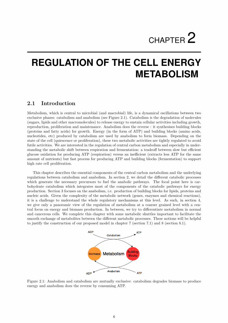
2.1 IntroductionMetabolism, which is central to microbial (and macrobial) life, is a dynamical oscillations between twoexclusive phases: catabolism and anabolism (see Figure 2.1). Catabolism is the degradation of molecules(sugars, lipids and other macromolecules) to release energy to sustain cellular activities including growth,reproduction, proliferation and maintenance. Anabolism does the reverse : it synthesises building blocks(proteins and fatty acids) for growth. Energy (in the form of ATP) and building blocks (amino acids,nucleotides, etc) produced by catabolism are used by anabolism to form biomass. Depending on thestate of the cell (quiescence or proliferation), these two metabolic activities are tightly regulated to avoidfutile activities. We are interested in the regulation of central carbon metabolism and especially in under-standing the metabolic shift between respiration and fermentation: a tradeoff between slow but efficientglucose oxidation for producing ATP (respiration) versus an inefficient (extracts less ATP for the sameamount of nutrients) but fast process for producing ATP and building blocks (fermentation) to supporthigh rate cell proliferation.
This chapter describes the essential components of the central carbon metabolism and the underlyingregulations between catabolism and anabolism. In section 2, we detail the different catabolic processeswhich generate the necessary precursors to fuel the anabolic pathways. The focal point here is car-bohydrate catabolism which integrates most of the components of the catabolic pathways for energyproduction. Section 3 focuses on the anabolism, i.e. production of building blocks for lipids, proteins andnucleic acids. Given the complexity of the metabolic network (genes, enzymes and chemical reactions),it is a challenge to understand the whole regulatory mechanisms at this level. As such, in section 4,we give only a panoramic view of the regulation of metabolism at a coarser grained level with a cen-tral focus on energy and biomass production. In between, we try to differentiate metabolism in normaland cancerous cells. We complete this chapter with some metabolic shuttles important to facilitate thesmooth exchange of metabolites between the different metabolic processes. These notions will be helpfulto justify the construction of our proposed model in chapter 7 (section 7.1) and 8 (section 8.1).
Figure 2.1: Anabolism and catabolism are mutually exclusive: catabolism degrades biomass to produceenergy and anabolism does the reverse by consuming ATP.
6
7 2.2. Catabolism
2.2 CatabolismCatabolism is a trade-off between the production of ATP and the production of building blocks. Dealingwith this trade-off is a matter of whether the cell is in quiescence or proliferative modes. Cells havetwo possible pathways for ATP production and generating building blocks: respiration and fermentation.Respiration occurs only in the presence of oxygen. It is a slow machinery that generates the majorityof ATP the cells require. The fermentative pathway has a double meaning: it can occur in the absenceof oxygen but it can also occur in the presence of oxygen under other cellular conditions. Moreover,it is faster process with a smaller yield of ATP production than respiration. Cells have the necessarymechanisms to switch between respiration and fermentation. This metabolic plasticity enables cell tosurvive in stressful conditions. In this text, the main nutrients that we use take the form of glucose, fattyacids and nitrogen & carbon donors, and they are discussed in next section.
2.2.1 Nutrients2.2.1.1 Dual view of nutrients
Nutrients captures a different meaning as we pass from the cell metabolism description to understand-ing of human physiology in which case, nutrition and diets are more suitable terms. They capture thefirst notion of fuel for the organism for which cellular central carbon metabolism is the core machinery.As regulation is concerned whether at the cellular level or at the physiological level in case of evolvedorganisms such as humans, nutrients refer also to molecular controllers (e.g. minerals, vitamins, neu-traceutics, drugs) that regulate the whole human physiology. The understanding of the interconnectionbetween the various hierarchical levels from cell metabolism to the control of homeostasis is the core ofsystemic pharmacology. In this context, nutrients play the role of molecular bio-indicators of various cellmetabolic regimes as well as dysregulated homoeostasis that explain the appearance of disease-relatedphenotypes such as glucose level in diabetes and cancer. This is possible with PET-scan (PET) whichallows the visualisation of glycolytic activity in vivo [19] and helps the diagnosis of cancer and tumors.As the understanding of these inter-hierarchical relations is beyond the scope of this study, we considernutrients in this chapter as cellular food for energy and biomass production.
Two primary elements crucial for cells are carbon and nitrogen, which in our study, come at differentlevels, in the form of glucose, fatty acids and nitrogen/carbon donors. These nutrients contribute tomost of the cellular carbon sources used for biogenesis [4]. Glucose catabolism generates ATP, NADPHand other biomasses for reductant biosynthesis and ROS detoxification. In association with the TCAcycle, glutamine (a major nitrogen & carbon donor) metabolism provides not only a carbon source butalso NADH, NH3+ (nitrogen sources) and other essential intermediates for lipid biosynthesis, amino acidsynthesis [4], and cellular acid detoxification. Fatty acids are precursors for lipid synthesis. Therefore,glucose, NCD, AA and FA seems to universally be the most critical nutrients for the growth and prolifer-ation of both normal and cancer cells. These nutrients are explained in this section and their metabolicimportance are highlighted.
2.2.1.2 Sugar, lipids and amino acids (glutamine) as carbon sources
At the cellular level, the primary element for biomass production is carbon for which sugars and lipidsare the more abundant sources. Central carbon metabolism is perfectly adapted to produce energy fromthese nutrients. Proteins are also carbon sources, and secondary pathways exist to replenish primaryoxidative pathways that oxidize glucose into CO2 to produce energy (ATP).
Sugars and lipids represent a reservoir of electrons and protons through the associated hydrogen atoms.The electron content of carbon within sugar and lipids or any molecules is a quality index for thesemolecules to produce ATP from electro-chemical energy. This can be estimated as the average of theredox states of each carbon atom of the molecule that ranges from -4 for CH4 to +4 for CO2. Glucoseand lipids have an average redox state of 0 and -2 respectively. Lipids are therefore more energetic peratom of carbon. This explains the energetical yield of these two molecules after complete oxidation of+34 ATP produced per molecule glucose and +143 ATP per molecule of palmitic acids.
8 2.2. Catabolism
2.2.1.3 Glutamine as a major nitrogen and carbon sources
The degradation of glutamine to provide nitrogen and carbon sources follows two possible pathways:an oxidative pathway representing the normal Krebs cycle (&Keto-Glutarate to malate) and a reductivepathway where glutamine is reduced to glutamate to do a reverse Krebs cycle to convert &Keto-Glutarateto citrate. The second most important atom after carbon is nitrogen which is, in particular, useful forthe composition of nucleic acids and alpha amino acids. Glutamine is the most abundant amino acids inplasma (20%) and in muscle (40%), and represents the major source of nitrogen for purine and pyrimidinesbiosynthesis in organs [5]. In cultures, tumor cells metabolise glutamine faster than any other aminoacids. However, only a small fraction of glutamine is used for nucleotides synthesis [6]. It plays a crucialrole in lipid synthesis as well, which makes glutaminolysis the major component of the metabolism ofproliferating cancer cells [7]. In this text, we use a more global name, NCD, to regroup all forms ofnitrogen and carbon donors.
2.2.1.4 Other nutrients
Other atoms enter into the constitution of cells and may play a crucial role in redox, pH homeostasisas certain ions in osmosis regulation. These take the form of proteins, vitamins, minerals and water.The systemic understanding of the different homeostasis is certainly explained through physiochemicalconsiderations through thermodynamics equilibrium and kinetics constants, and the regulation rules referto a much finer granularity which is also beyond the scope of this study. These effects are therefore notexplicitly taken into account in our model. All these essentials atoms or constituents are however notconsidered as a cell carburant as sugars and lipids does, unless in certain bacteria in which ammoniumions (reduced form of nitrogen) serve as reservoir of electrons.
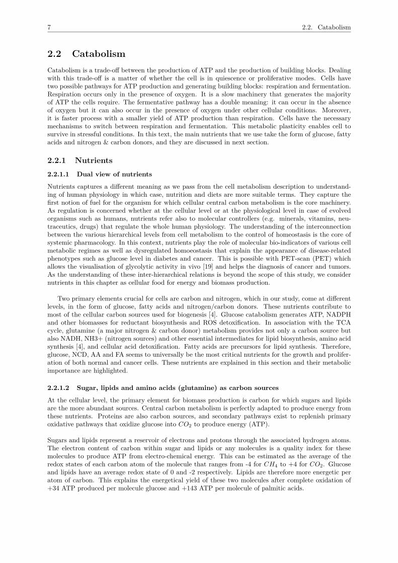
2.2.2 GlycolysisThe degradation of the 6-carbon glucose in the cytosol inside cells is a quintessential step of glycolysis,which is a precondition for either fermentation or respiration. After its intake by enzymes (GLUT1 andGLUT2; also called glucose transporters; in neurons, GLUT3 does this) through cell membranes, glucoseundergoes a series of oxidative-reductive steps to be finally transformed into the 3-carbon molecule,pyruvate (see Figure 2.2).
2.2.2.1 A global view
Pyruvate is at the bifurcation point of two main pathways of carbon metabolism: fermentation and res-piration. Under the presence of oxygen, pyruvate enters the TCA (TriCarboxylic Acid) or Krebs cycleto complete its oxidative degradation via the respiratory pathway. In hypoxia (<2% vol of oxygen),pyruvate is reduced into lactate or ethanol depending on the organism. The fermentation pathway inour semantic is constituted of a single enzyme, Lactate Dehydrogenase (LDH) in humans for example orAlcohol Dehydrogenase (ADH) in Saccharomyces Cerevisiae, for example.Cells obtain their initial dose of energy through this pathway which is equivalent to a net of 2 ATP (2molecules are consumed initially and 4 ATP are produced at the end of the glycolytic pathway). This isaccompanied by a parallel production of 2 NADH where the compound Glyceraldehyde 3-phosphate(G3P)is converted in a multitude of steps to produce pyruvate. The enzyme Glyceraldehyde 3-phosphate dehy-drogenase (commonly abbreviated as GAPDH) is involved during this conversion of NAD+ to NADH.
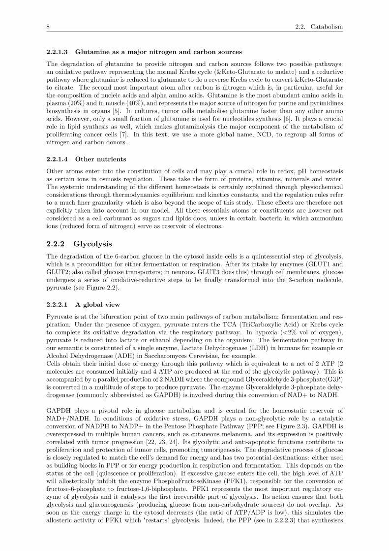
GAPDH plays a pivotal role in glucose metabolism and is central for the homeostatic reservoir ofNAD+/NADH. In conditions of oxidative stress, GAPDH plays a non-glycolytic role by a catalyticconversion of NADPH to NADP+ in the Pentose Phosphate Pathway (PPP; see Figure 2.3). GAPDH isoverexpressed in multiple human cancers, such as cutaneous melanoma, and its expression is positivelycorrelated with tumor progression [22, 23, 24]. Its glycolytic and anti-apoptotic functions contribute toproliferation and protection of tumor cells, promoting tumorigenesis. The degradative process of glucoseis closely regulated to match the cell’s demand for energy and has two potential destinations: either usedas building blocks in PPP or for energy production in respiration and fermentation. This depends on thestatus of the cell (quiescence or proliferation). If excessive glucose enters the cell, the high level of ATPwill allosterically inhibit the enzyme PhosphoFructoseKinase (PFK1), responsible for the conversion offructose-6-phosphate to fructose-1,6-biphosphate. PFK1 represents the most important regulatory en-zyme of glycolysis and it catalyses the first irreversible part of glycolysis. Its action ensures that bothglycolysis and gluconeogenesis (producing glucose from non-carbohydrate sources) do not overlap. Assoon as the energy charge in the cytosol decreases (the ratio of ATP/ADP is low), this simulates theallosteric activity of PFK1 which "restarts" glycolysis. Indeed, the PPP (see in 2.2.2.3) that synthesises
9 2.2. Catabolism
the precursors of biomass (nucleic acids, amino acids) has its root just above PFK1, using G6P as astarting point. Therefore, PFK1 regulates the cellular fate between production of precursor or ATPgeneration for glycolysis. As long as cells receive glucose nutrient, they will churn out ATP endlessly forsustainability reasons.
Figure 2.2: Glycolysis: A catabolic process producing ATP, NADH and pyruvate, and some precursorsfor Pentose Phosphate Pathway (PPP)
Figure 2.3: GADPH plays a double role in cytoplasmic metabolism: Glycolytic (conversion of NAD+ toNADH) and non-glycolytic (conversion of NADPH to NADP+)
In tumour cells, fermentation occurs even in presence of oxygen and under high supply of glucose asobserved by O. Warburg in 1922 and later in 1929 by H. Crabtree for bacteria. This transition fromrespiration to fermentation is referred to as the Warburg/Crabtree effect. We will not differentiate inthis study the long term irreversibility and the short term reversibility character of these two effects.The reversibility can be observed in facultative fermentative aerobes (e.g. Saccharomyces Cerevisiae)when changing from rich milieu to deficient glucose supply. Beside the production of ATP, glycolysisprovides the intermediate metabolites for building blocks synthesis that will be used during anabolismfor biomass production. The two main anabolic pathways directly connected to glycolysis is the PPPwith glucose-6-phosphate (G6P) as entry point and the serine biosynthesis pathway which takes place atthe level of 3-phosphoglycerate.
10 2.2. Catabolism
The use of glucose for building block synthesis is favored in tumour cells by an increased intakeof glucose through over expression of glucose receptors (GLUT) and by increasing glycolytic flux, anddivergence towards anabolic pathways by modifying the thermodynamics balance through metaboliteaccumulation.
2.2.2.2 ATP production
In the first part of glycolysis, cells invest energy dispense that prevent glucose efflux: a first phosphoryla-tion, consuming 1 ATP is realized by hexokinase. It prevents glucose exit by diffusion into the membrane.A second phosphorylation consuming also 1 ATP is realized by Phosphofructokinase (PFK1,2). Thesetwo phosphorylation on alcohol groups are expensive and are made at the expense of 2 ATP. The fruc-tose 1,6-biphosphate is then cleaved into two C3 molecules that are half phosphorylated. Here comesthe nice trick of glycolysis to make ROI (Return of Investment): to be able to produce 2 ATP per C3intermediates, the cell phosphorylates each intermediate with an additional inorganic phosphate. Forthis cheap reaction to happen in terms of electrochemical energy, alcohol is first oxidized into aldehyde (atoxic intermediate) with ionization state of aldehyde carbon = +1 which favors the oxidation by organicphosphate. The last step of glycolysis is the energy production stage: the two Glycerate 1,3 biphosphateare now the substrate for ATP production, 2 ATP per intermediate, that is, 4 ATP in total per moleculeof glucose. The second phosphorylation with inorganic Phosphate (Pi) is less costly energetically thanphosphorylation of alcohol group. The coupled reduction of NAD+ into NADH+ provides the necessaryelectrochemical energy for this phosphorylation. As this reaction consumes 2 protons, the energetic yieldof glycolysis is expected to be favoured under acidic conditions.
2.2.2.3 A building block synthetic pathway: PPP
The Pentose Phosphate Pathway is a maintenance pathway that occurs in the cytoplasm and accountsfor the formation of the reducing agent NADPH and precursors for the production of biomass. PPPis tightly connected to glycolysis (see Figure 2.4). Some glucose-6-phosphate molecules "leak" from theglycolytic pathway to be used as a first substrate in PPP. It undergoes two types of metabolism in thePPP: oxidative and non-oxidative branches. The oxidative branch includes a series of non-reversibleconversions of glucose-6-phosphate to ribulose-5P essential for nucleic acid synthesis. At the same time,NADP+ is converted to NADPH, which has a crucial role in cancer cells as it relieves them from oxidativestress during ROS (using glutathione reductase to maintain redox state of cell). Thus, NADPH is a goodscavenger but is also known for participating meagrely in fatty acids synthesis. NADPH homeostasisis critical for cancer cells in starved microenvironments. The non-oxidative segment produces glucosederivatives like fructose-6-phosphate and which are reused in glycolysis. Interestingly, the potentiality ofPPP has been demonstrated in disease like sleeping sickness [8, 9].
It has become clear that the PPP plays a critical role in regulating cancer cell growth by supplyingcells with not only ribose-5-phosphate but also NADPH for detoxification of intracellular reactive oxygenspecies, reductive biosynthesis and ribose biogenesis. Thus, alteration of the PPP contributes directly tocell proliferation, survival and senescence. Dysregulation of PPP flux dramatically impacts cancer growthand survival. PPP is both positively and negatively regulated by numerous factors as shown in Figure 2.5.Therefore, a better understanding of how the PPP is reprogrammed and the mechanism underlying thebalance between glycolysis and PPP flux in cancer could be valuable in developing therapeutic strategiestargeting this pathway.
The tumour suppressor, p53, is the most frequently mutated gene in human tumours and has beenshown to inhibit PPP. Through the PPP, p53 suppresses glucose consumption, NADPH production andbiosynthesis. Tumour-associated p53 mutants lack the G6PD-inhibitory activity. Therefore, enhancedPPP glucose flux due to p53 inactivation may increase glucose consumption and direct glucose towardsbiosynthesis in tumour cells [11, 12]. p53 deficiency reduces the expression of TIGAR, which has a role insuppressing glycolysis by lowering intracellular levels of fructose-2,6-bisphosphate (F-2,6-P2). F-2,6-P2is a strong allosteric activator of phosphofructokinse-1 (PFK1), and the reduction of F-2,6-P2 results indecreased PFK1 activity and glycolytic flux [11]. p53 suppresses the PPP by directly binding to G6PDand repressing its enzyme activity. However, the ability to inhibit G6PD is restricted to wild type p53.To conclude, it can be hypothesized that in cancer cells, p53 mutations may liberate G6PD and activatePFK1, causing increased PPP flux and glycolysis.
11 2.2. Catabolism
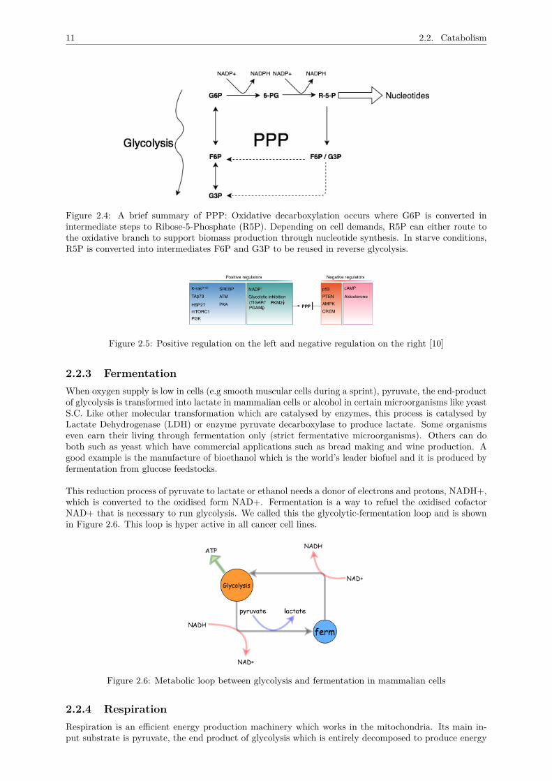
Figure 2.4: A brief summary of PPP: Oxidative decarboxylation occurs where G6P is converted inintermediate steps to Ribose-5-Phosphate (R5P). Depending on cell demands, R5P can either route tothe oxidative branch to support biomass production through nucleotide synthesis. In starve conditions,R5P is converted into intermediates F6P and G3P to be reused in reverse glycolysis.
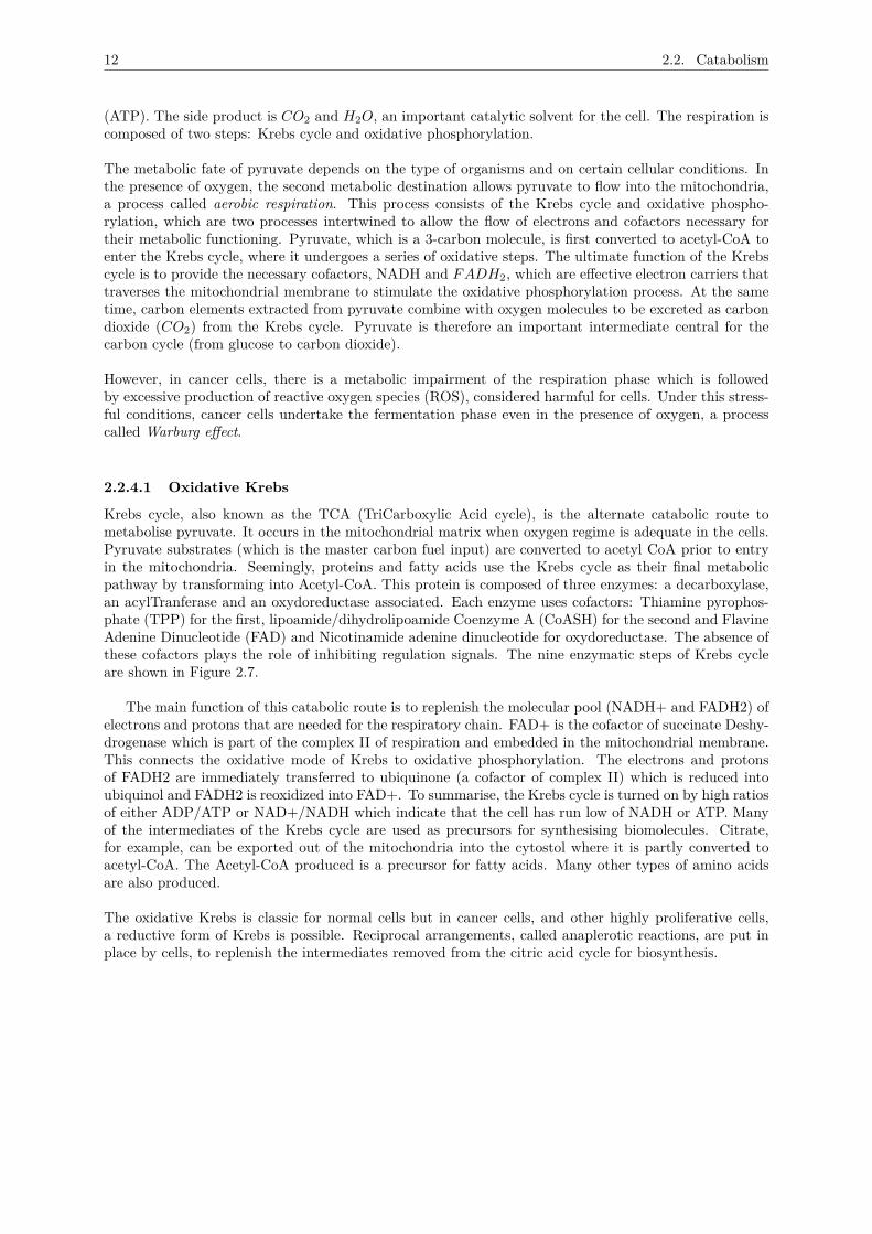
Figure 2.5: Positive regulation on the left and negative regulation on the right [10]
2.2.3 FermentationWhen oxygen supply is low in cells (e.g smooth muscular cells during a sprint), pyruvate, the end-productof glycolysis is transformed into lactate in mammalian cells or alcohol in certain microorganisms like yeastS.C. Like other molecular transformation which are catalysed by enzymes, this process is catalysed byLactate Dehydrogenase (LDH) or enzyme pyruvate decarboxylase to produce lactate. Some organismseven earn their living through fermentation only (strict fermentative microorganisms). Others can doboth such as yeast which have commercial applications such as bread making and wine production. Agood example is the manufacture of bioethanol which is the world’s leader biofuel and it is produced byfermentation from glucose feedstocks.
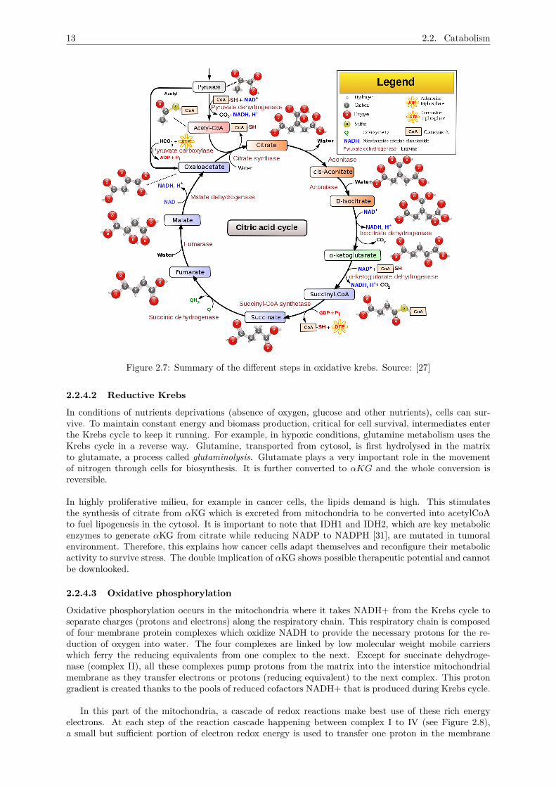
This reduction process of pyruvate to lactate or ethanol needs a donor of electrons and protons, NADH+,which is converted to the oxidised form NAD+. Fermentation is a way to refuel the oxidised cofactorNAD+ that is necessary to run glycolysis. We called this the glycolytic-fermentation loop and is shownin Figure 2.6. This loop is hyper active in all cancer cell lines.
Figure 2.6: Metabolic loop between glycolysis and fermentation in mammalian cells
2.2.4 RespirationRespiration is an efficient energy production machinery which works in the mitochondria. Its main in-put substrate is pyruvate, the end product of glycolysis which is entirely decomposed to produce energy
12 2.2. Catabolism
(ATP). The side product is CO2 and H2O, an important catalytic solvent for the cell. The respiration iscomposed of two steps: Krebs cycle and oxidative phosphorylation.
The metabolic fate of pyruvate depends on the type of organisms and on certain cellular conditions. Inthe presence of oxygen, the second metabolic destination allows pyruvate to flow into the mitochondria,a process called aerobic respiration. This process consists of the Krebs cycle and oxidative phospho-rylation, which are two processes intertwined to allow the flow of electrons and cofactors necessary fortheir metabolic functioning. Pyruvate, which is a 3-carbon molecule, is first converted to acetyl-CoA toenter the Krebs cycle, where it undergoes a series of oxidative steps. The ultimate function of the Krebscycle is to provide the necessary cofactors, NADH and FADH2, which are effective electron carriers thattraverses the mitochondrial membrane to stimulate the oxidative phosphorylation process. At the sametime, carbon elements extracted from pyruvate combine with oxygen molecules to be excreted as carbondioxide (CO2) from the Krebs cycle. Pyruvate is therefore an important intermediate central for thecarbon cycle (from glucose to carbon dioxide).
However, in cancer cells, there is a metabolic impairment of the respiration phase which is followedby excessive production of reactive oxygen species (ROS), considered harmful for cells. Under this stress-ful conditions, cancer cells undertake the fermentation phase even in the presence of oxygen, a processcalled Warburg effect.
2.2.4.1 Oxidative Krebs
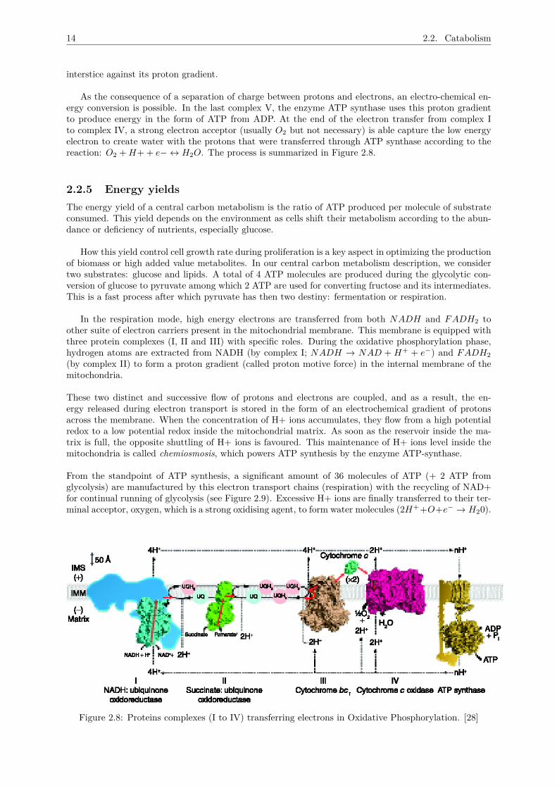
Krebs cycle, also known as the TCA (TriCarboxylic Acid cycle), is the alternate catabolic route tometabolise pyruvate. It occurs in the mitochondrial matrix when oxygen regime is adequate in the cells.Pyruvate substrates (which is the master carbon fuel input) are converted to acetyl CoA prior to entryin the mitochondria. Seemingly, proteins and fatty acids use the Krebs cycle as their final metabolicpathway by transforming into Acetyl-CoA. This protein is composed of three enzymes: a decarboxylase,an acylTranferase and an oxydoreductase associated. Each enzyme uses cofactors: Thiamine pyrophos-phate (TPP) for the first, lipoamide/dihydrolipoamide Coenzyme A (CoASH) for the second and FlavineAdenine Dinucleotide (FAD) and Nicotinamide adenine dinucleotide for oxydoreductase. The absence ofthese cofactors plays the role of inhibiting regulation signals. The nine enzymatic steps of Krebs cycleare shown in Figure 2.7.
The main function of this catabolic route is to replenish the molecular pool (NADH+ and FADH2) ofelectrons and protons that are needed for the respiratory chain. FAD+ is the cofactor of succinate Deshy-drogenase which is part of the complex II of respiration and embedded in the mitochondrial membrane.This connects the oxidative mode of Krebs to oxidative phosphorylation. The electrons and protonsof FADH2 are immediately transferred to ubiquinone (a cofactor of complex II) which is reduced intoubiquinol and FADH2 is reoxidized into FAD+. To summarise, the Krebs cycle is turned on by high ratiosof either ADP/ATP or NAD+/NADH which indicate that the cell has run low of NADH or ATP. Manyof the intermediates of the Krebs cycle are used as precursors for synthesising biomolecules. Citrate,for example, can be exported out of the mitochondria into the cytostol where it is partly converted toacetyl-CoA. The Acetyl-CoA produced is a precursor for fatty acids. Many other types of amino acidsare also produced.
The oxidative Krebs is classic for normal cells but in cancer cells, and other highly proliferative cells,a reductive form of Krebs is possible. Reciprocal arrangements, called anaplerotic reactions, are put inplace by cells, to replenish the intermediates removed from the citric acid cycle for biosynthesis.
13 2.2. Catabolism
Figure 2.7: Summary of the different steps in oxidative krebs. Source: [27]
2.2.4.2 Reductive Krebs
In conditions of nutrients deprivations (absence of oxygen, glucose and other nutrients), cells can sur-vive. To maintain constant energy and biomass production, critical for cell survival, intermediates enterthe Krebs cycle to keep it running. For example, in hypoxic conditions, glutamine metabolism uses theKrebs cycle in a reverse way. Glutamine, transported from cytosol, is first hydrolysed in the matrixto glutamate, a process called glutaminolysis. Glutamate plays a very important role in the movementof nitrogen through cells for biosynthesis. It is further converted to αKG and the whole conversion isreversible.
In highly proliferative milieu, for example in cancer cells, the lipids demand is high. This stimulatesthe synthesis of citrate from αKG which is excreted from mitochondria to be converted into acetylCoAto fuel lipogenesis in the cytosol. It is important to note that IDH1 and IDH2, which are key metabolicenzymes to generate αKG from citrate while reducing NADP to NADPH [31], are mutated in tumoralenvironment. Therefore, this explains how cancer cells adapt themselves and reconfigure their metabolicactivity to survive stress. The double implication of αKG shows possible therapeutic potential and cannotbe downlooked.
2.2.4.3 Oxidative phosphorylation
Oxidative phosphorylation occurs in the mitochondria where it takes NADH+ from the Krebs cycle toseparate charges (protons and electrons) along the respiratory chain. This respiratory chain is composedof four membrane protein complexes which oxidize NADH to provide the necessary protons for the re-duction of oxygen into water. The four complexes are linked by low molecular weight mobile carrierswhich ferry the reducing equivalents from one complex to the next. Except for succinate dehydroge-nase (complex II), all these complexes pump protons from the matrix into the interstice mitochondrialmembrane as they transfer electrons or protons (reducing equivalent) to the next complex. This protongradient is created thanks to the pools of reduced cofactors NADH+ that is produced during Krebs cycle.
In this part of the mitochondria, a cascade of redox reactions make best use of these rich energyelectrons. At each step of the reaction cascade happening between complex I to IV (see Figure 2.8),a small but sufficient portion of electron redox energy is used to transfer one proton in the membrane
14 2.2. Catabolism
interstice against its proton gradient.
As the consequence of a separation of charge between protons and electrons, an electro-chemical en-ergy conversion is possible. In the last complex V, the enzyme ATP synthase uses this proton gradientto produce energy in the form of ATP from ADP. At the end of the electron transfer from complex Ito complex IV, a strong electron acceptor (usually O2 but not necessary) is able capture the low energyelectron to create water with the protons that were transferred through ATP synthase according to thereaction: O2 +H+ + e− ↔ H2O. The process is summarized in Figure 2.8.
2.2.5 Energy yieldsThe energy yield of a central carbon metabolism is the ratio of ATP produced per molecule of substrateconsumed. This yield depends on the environment as cells shift their metabolism according to the abun-dance or deficiency of nutrients, especially glucose.
How this yield control cell growth rate during proliferation is a key aspect in optimizing the productionof biomass or high added value metabolites. In our central carbon metabolism description, we considertwo substrates: glucose and lipids. A total of 4 ATP molecules are produced during the glycolytic con-version of glucose to pyruvate among which 2 ATP are used for converting fructose and its intermediates.This is a fast process after which pyruvate has then two destiny: fermentation or respiration.
In the respiration mode, high energy electrons are transferred from both NADH and FADH2 toother suite of electron carriers present in the mitochondrial membrane. This membrane is equipped withthree protein complexes (I, II and III) with specific roles. During the oxidative phosphorylation phase,hydrogen atoms are extracted from NADH (by complex I; NADH → NAD + H+ + e−) and FADH2(by complex II) to form a proton gradient (called proton motive force) in the internal membrane of themitochondria.
These two distinct and successive flow of protons and electrons are coupled, and as a result, the en-ergy released during electron transport is stored in the form of an electrochemical gradient of protonsacross the membrane. When the concentration of H+ ions accumulates, they flow from a high potentialredox to a low potential redox inside the mitochondrial matrix. As soon as the reservoir inside the ma-trix is full, the opposite shuttling of H+ ions is favoured. This maintenance of H+ ions level inside themitochondria is called chemiosmosis, which powers ATP synthesis by the enzyme ATP-synthase.
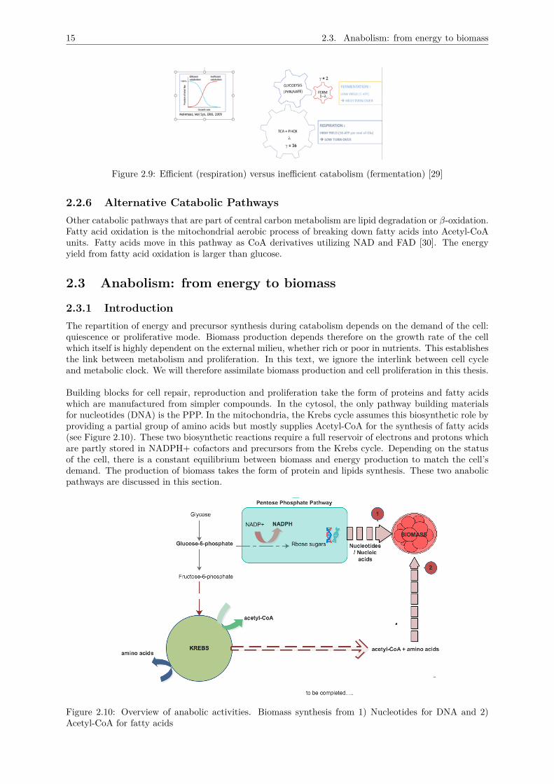
From the standpoint of ATP synthesis, a significant amount of 36 molecules of ATP (+ 2 ATP fromglycolysis) are manufactured by this electron transport chains (respiration) with the recycling of NAD+for continual running of glycolysis (see Figure 2.9). Excessive H+ ions are finally transferred to their ter-minal acceptor, oxygen, which is a strong oxidising agent, to form water molecules (2H++O+e− → H20).
Figure 2.8: Proteins complexes (I to IV) transferring electrons in Oxidative Phosphorylation. [28]
15 2.3. Anabolism: from energy to biomass
Figure 2.9: Efficient (respiration) versus inefficient catabolism (fermentation) [29]
2.2.6 Alternative Catabolic PathwaysOther catabolic pathways that are part of central carbon metabolism are lipid degradation or β-oxidation.Fatty acid oxidation is the mitochondrial aerobic process of breaking down fatty acids into Acetyl-CoAunits. Fatty acids move in this pathway as CoA derivatives utilizing NAD and FAD [30]. The energyyield from fatty acid oxidation is larger than glucose.
2.3 Anabolism: from energy to biomass
2.3.1 IntroductionThe repartition of energy and precursor synthesis during catabolism depends on the demand of the cell:quiescence or proliferative mode. Biomass production depends therefore on the growth rate of the cellwhich itself is highly dependent on the external milieu, whether rich or poor in nutrients. This establishesthe link between metabolism and proliferation. In this text, we ignore the interlink between cell cycleand metabolic clock. We will therefore assimilate biomass production and cell proliferation in this thesis.
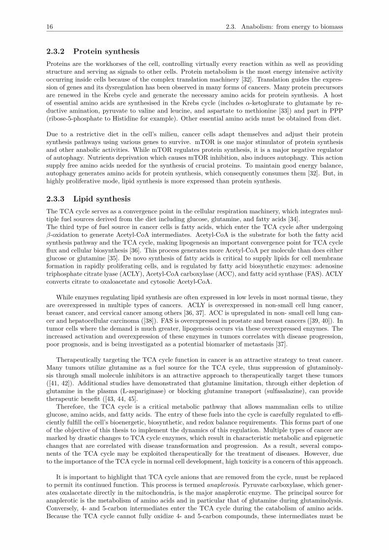
Building blocks for cell repair, reproduction and proliferation take the form of proteins and fatty acidswhich are manufactured from simpler compounds. In the cytosol, the only pathway building materialsfor nucleotides (DNA) is the PPP. In the mitochondria, the Krebs cycle assumes this biosynthetic role byproviding a partial group of amino acids but mostly supplies Acetyl-CoA for the synthesis of fatty acids(see Figure 2.10). These two biosynthetic reactions require a full reservoir of electrons and protons whichare partly stored in NADPH+ cofactors and precursors from the Krebs cycle. Depending on the statusof the cell, there is a constant equilibrium between biomass and energy production to match the cell’sdemand. The production of biomass takes the form of protein and lipids synthesis. These two anabolicpathways are discussed in this section.
Figure 2.10: Overview of anabolic activities. Biomass synthesis from 1) Nucleotides for DNA and 2)Acetyl-CoA for fatty acids
16 2.3. Anabolism: from energy to biomass
2.3.2 Protein synthesisProteins are the workhorses of the cell, controlling virtually every reaction within as well as providingstructure and serving as signals to other cells. Protein metabolism is the most energy intensive activityoccurring inside cells because of the complex translation machinery [32]. Translation guides the expres-sion of genes and its dysregulation has been observed in many forms of cancers. Many protein precursorsare renewed in the Krebs cycle and generate the necessary amino acids for protein synthesis. A hostof essential amino acids are synthesised in the Krebs cycle (includes α-ketoglurate to glutamate by re-ductive amination, pyruvate to valine and leucine, and aspartate to methionine [33]) and part in PPP(ribose-5-phosphate to Histidine for example). Other essential amino acids must be obtained from diet.
Due to a restrictive diet in the cell’s milieu, cancer cells adapt themselves and adjust their proteinsynthesis pathways using various genes to survive. mTOR is one major stimulator of protein synthesisand other anabolic activities. While mTOR regulates protein synthesis, it is a major negative regulatorof autophagy. Nutrients deprivation which causes mTOR inhibition, also induces autophagy. This actionsupply free amino acids needed for the synthesis of crucial proteins. To maintain good energy balance,autophagy generates amino acids for protein synthesis, which consequently consumes them [32]. But, inhighly proliferative mode, lipid synthesis is more expressed than protein synthesis.
2.3.3 Lipid synthesisThe TCA cycle serves as a convergence point in the cellular respiration machinery, which integrates mul-tiple fuel sources derived from the diet including glucose, glutamine, and fatty acids [34].The third type of fuel source in cancer cells is fatty acids, which enter the TCA cycle after undergoingβ-oxidation to generate Acetyl-CoA intermediates. Acetyl-CoA is the substrate for both the fatty acidsynthesis pathway and the TCA cycle, making lipogenesis an important convergence point for TCA cycleflux and cellular biosynthesis [36]. This process generates more Acetyl-CoA per molecule than does eitherglucose or glutamine [35]. De novo synthesis of fatty acids is critical to supply lipids for cell membraneformation in rapidly proliferating cells, and is regulated by fatty acid biosynthetic enzymes: adenosinetriphosphate citrate lyase (ACLY), Acetyl-CoA carboxylase (ACC), and fatty acid synthase (FAS). ACLYconverts citrate to oxaloacetate and cytosolic Acetyl-CoA.
While enzymes regulating lipid synthesis are often expressed in low levels in most normal tissue, theyare overexpressed in multiple types of cancers. ACLY is overexpressed in non-small cell lung cancer,breast cancer, and cervical cancer among others [36, 37]. ACC is upregulated in non- small cell lung can-cer and hepatocellular carcinoma ([38]). FAS is overexpressed in prostate and breast cancers ([39, 40]). Intumor cells where the demand is much greater, lipogenesis occurs via these overexpressed enzymes. Theincreased activation and overexpression of these enzymes in tumors correlates with disease progression,poor prognosis, and is being investigated as a potential biomarker of metastasis [37].
Therapeutically targeting the TCA cycle function in cancer is an attractive strategy to treat cancer.Many tumors utilize glutamine as a fuel source for the TCA cycle, thus suppression of glutaminoly-sis through small molecule inhibitors is an attractive approach to therapeutically target these tumors([41, 42]). Additional studies have demonstrated that glutamine limitation, through either depletion ofglutamine in the plasma (L-aspariginase) or blocking glutamine transport (sulfasalazine), can providetherapeutic benefit ([43, 44, 45].
Therefore, the TCA cycle is a critical metabolic pathway that allows mammalian cells to utilizeglucose, amino acids, and fatty acids. The entry of these fuels into the cycle is carefully regulated to effi-ciently fulfill the cell’s bioenergetic, biosynthetic, and redox balance requirements. This forms part of oneof the objective of this thesis to implement the dynamics of this regulation. Multiple types of cancer aremarked by drastic changes to TCA cycle enzymes, which result in characteristic metabolic and epigeneticchanges that are correlated with disease transformation and progression. As a result, several compo-nents of the TCA cycle may be exploited therapeutically for the treatment of diseases. However, dueto the importance of the TCA cycle in normal cell development, high toxicity is a concern of this approach.
It is important to highlight that TCA cycle anions that are removed from the cycle, must be replacedto permit its continued function. This process is termed anaplerosis. Pyruvate carboxylase, which gener-ates oxalacetate directly in the mitochondria, is the major anaplerotic enzyme. The principal source foranaplerotic is the metabolism of amino acids and in particular that of glutamine during glutaminolysis.Conversely, 4- and 5-carbon intermediates enter the TCA cycle during the catabolism of amino acids.Because the TCA cycle cannot fully oxidize 4- and 5-carbon compounds, these intermediates must be
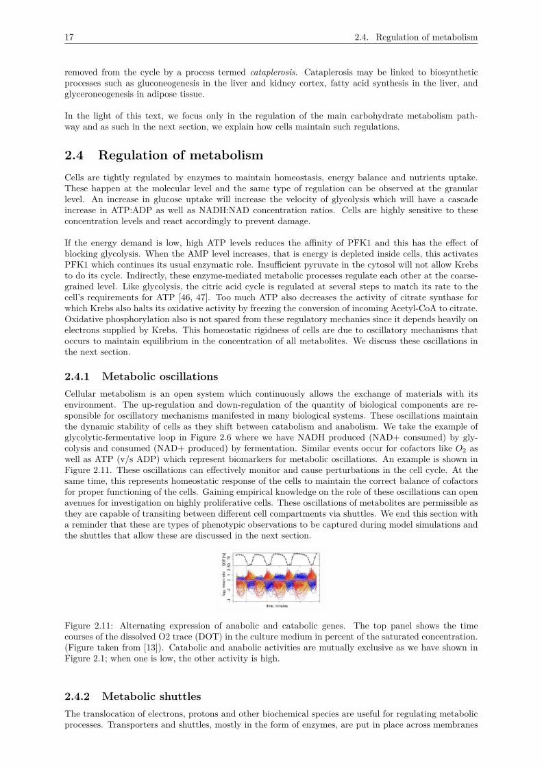
17 2.4. Regulation of metabolism
removed from the cycle by a process termed cataplerosis. Cataplerosis may be linked to biosyntheticprocesses such as gluconeogenesis in the liver and kidney cortex, fatty acid synthesis in the liver, andglyceroneogenesis in adipose tissue.
In the light of this text, we focus only in the regulation of the main carbohydrate metabolism path-way and as such in the next section, we explain how cells maintain such regulations.
2.4 Regulation of metabolismCells are tightly regulated by enzymes to maintain homeostasis, energy balance and nutrients uptake.These happen at the molecular level and the same type of regulation can be observed at the granularlevel. An increase in glucose uptake will increase the velocity of glycolysis which will have a cascadeincrease in ATP:ADP as well as NADH:NAD concentration ratios. Cells are highly sensitive to theseconcentration levels and react accordingly to prevent damage.
If the energy demand is low, high ATP levels reduces the affinity of PFK1 and this has the effect ofblocking glycolysis. When the AMP level increases, that is energy is depleted inside cells, this activatesPFK1 which continues its usual enzymatic role. Insufficient pyruvate in the cytosol will not allow Krebsto do its cycle. Indirectly, these enzyme-mediated metabolic processes regulate each other at the coarse-grained level. Like glycolysis, the citric acid cycle is regulated at several steps to match its rate to thecell’s requirements for ATP [46, 47]. Too much ATP also decreases the activity of citrate synthase forwhich Krebs also halts its oxidative activity by freezing the conversion of incoming Acetyl-CoA to citrate.Oxidative phosphorylation also is not spared from these regulatory mechanics since it depends heavily onelectrons supplied by Krebs. This homeostatic rigidness of cells are due to oscillatory mechanisms thatoccurs to maintain equilibrium in the concentration of all metabolites. We discuss these oscillations inthe next section.
2.4.1 Metabolic oscillationsCellular metabolism is an open system which continuously allows the exchange of materials with itsenvironment. The up-regulation and down-regulation of the quantity of biological components are re-sponsible for oscillatory mechanisms manifested in many biological systems. These oscillations maintainthe dynamic stability of cells as they shift between catabolism and anabolism. We take the example ofglycolytic-fermentative loop in Figure 2.6 where we have NADH produced (NAD+ consumed) by gly-colysis and consumed (NAD+ produced) by fermentation. Similar events occur for cofactors like O2 aswell as ATP (v/s ADP) which represent biomarkers for metabolic oscillations. An example is shown inFigure 2.11. These oscillations can effectively monitor and cause perturbations in the cell cycle. At thesame time, this represents homeostatic response of the cells to maintain the correct balance of cofactorsfor proper functioning of the cells. Gaining empirical knowledge on the role of these oscillations can openavenues for investigation on highly proliferative cells. These oscillations of metabolites are permissible asthey are capable of transiting between different cell compartments via shuttles. We end this section witha reminder that these are types of phenotypic observations to be captured during model simulations andthe shuttles that allow these are discussed in the next section.
Figure 2.11: Alternating expression of anabolic and catabolic genes. The top panel shows the timecourses of the dissolved O2 trace (DOT) in the culture medium in percent of the saturated concentration.(Figure taken from [13]). Catabolic and anabolic activities are mutually exclusive as we have shown inFigure 2.1; when one is low, the other activity is high.
2.4.2 Metabolic shuttlesThe translocation of electrons, protons and other biochemical species are useful for regulating metabolicprocesses. Transporters and shuttles, mostly in the form of enzymes, are put in place across membranes
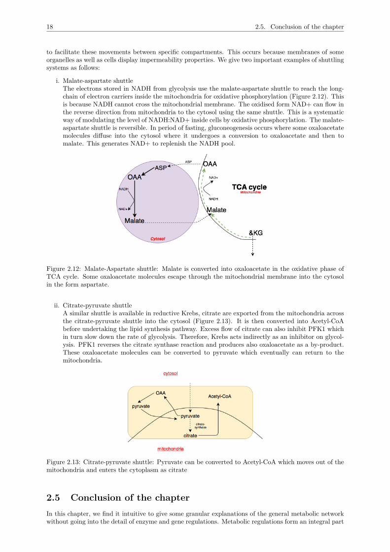
18 2.5. Conclusion of the chapter
to facilitate these movements between specific compartments. This occurs because membranes of someorganelles as well as cells display impermeability properties. We give two important examples of shuttlingsystems as follows:
i. Malate-aspartate shuttleThe electrons stored in NADH from glycolysis use the malate-aspartate shuttle to reach the long-chain of electron carriers inside the mitochondria for oxidative phosphorylation (Figure 2.12). Thisis because NADH cannot cross the mitochondrial membrane. The oxidised form NAD+ can flow inthe reverse direction from mitochondria to the cytosol using the same shuttle. This is a systematicway of modulating the level of NADH:NAD+ inside cells by oxidative phosphorylation. The malate-aspartate shuttle is reversible. In period of fasting, gluconeogenesis occurs where some oxaloacetatemolecules diffuse into the cytosol where it undergoes a conversion to oxaloacetate and then tomalate. This generates NAD+ to replenish the NADH pool.
Figure 2.12: Malate-Aspartate shuttle: Malate is converted into oxaloacetate in the oxidative phase ofTCA cycle. Some oxaloacetate molecules escape through the mitochondrial membrane into the cytosolin the form aspartate.
ii. Citrate-pyruvate shuttleA similar shuttle is available in reductive Krebs, citrate are exported from the mitochondria acrossthe citrate-pyruvate shuttle into the cytosol (Figure 2.13). It is then converted into Acetyl-CoAbefore undertaking the lipid synthesis pathway. Excess flow of citrate can also inhibit PFK1 whichin turn slow down the rate of glycolysis. Therefore, Krebs acts indirectly as an inhibitor on glycol-ysis. PFK1 reverses the citrate synthase reaction and produces also oxaloacetate as a by-product.These oxaloacetate molecules can be converted to pyruvate which eventually can return to themitochondria.
Figure 2.13: Citrate-pyruvate shuttle: Pyruvate can be converted to Acetyl-CoA which moves out of themitochondria and enters the cytoplasm as citrate
2.5 Conclusion of the chapterIn this chapter, we find it intuitive to give some granular explanations of the general metabolic networkwithout going into the detail of enzyme and gene regulations. Metabolic regulations form an integral part
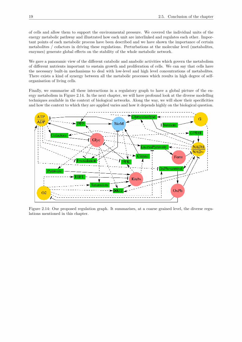
19 2.5. Conclusion of the chapter
of cells and allow them to support the environmental pressure. We covered the individual units of theenergy metabolic pathway and illustrated how each unit are interlinked and regulates each other. Impor-tant points of each metabolic process have been described and we have shown the importance of certainmetabolites / cofactors in driving these regulations. Perturbations at the molecular level (metabolites,enzymes) generate global effects on the stability of the whole metabolic network.
We gave a panoramic view of the different catabolic and anabolic activities which govern the metabolismof different nutrients important to sustain growth and proliferation of cells. We can say that cells havethe necessary built-in mechanisms to deal with low-level and high level concentrations of metabolites.There exists a kind of synergy between all the metabolic processes which results in high degree of self-organisation of living cells.
Finally, we summarise all these interactions in a regulatory graph to have a global picture of the en-ergy metabolism in Figure 2.14. In the next chapter, we will have profound look at the diverse modellingtechniques available in the context of biological networks. Along the way, we will show their specificitiesand how the context to which they are applied varies and how it depends highly on the biological question.
Figure 2.14: Our proposed regulation graph. It summarises, at a coarse grained level, the diverse regu-lations mentioned in this chapter.
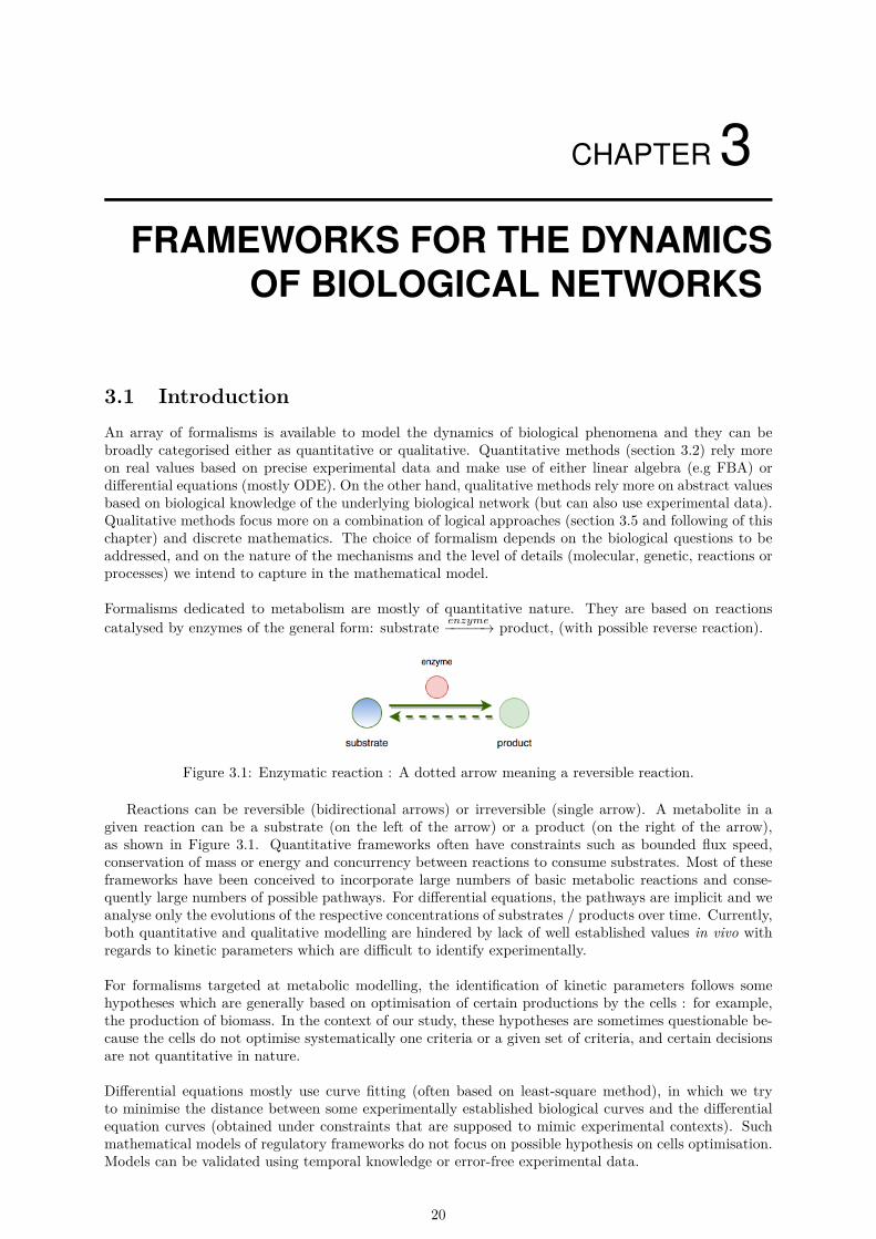
CHAPTER 3FRAMEWORKS FOR THE DYNAMICS
OF BIOLOGICAL NETWORKS
3.1 IntroductionAn array of formalisms is available to model the dynamics of biological phenomena and they can bebroadly categorised either as quantitative or qualitative. Quantitative methods (section 3.2) rely moreon real values based on precise experimental data and make use of either linear algebra (e.g FBA) ordifferential equations (mostly ODE). On the other hand, qualitative methods rely more on abstract valuesbased on biological knowledge of the underlying biological network (but can also use experimental data).Qualitative methods focus more on a combination of logical approaches (section 3.5 and following of thischapter) and discrete mathematics. The choice of formalism depends on the biological questions to beaddressed, and on the nature of the mechanisms and the level of details (molecular, genetic, reactions orprocesses) we intend to capture in the mathematical model.
Formalisms dedicated to metabolism are mostly of quantitative nature. They are based on reactionscatalysed by enzymes of the general form: substrate enzyme−−−−−→ product, (with possible reverse reaction).
Figure 3.1: Enzymatic reaction : A dotted arrow meaning a reversible reaction.
Reactions can be reversible (bidirectional arrows) or irreversible (single arrow). A metabolite in agiven reaction can be a substrate (on the left of the arrow) or a product (on the right of the arrow),as shown in Figure 3.1. Quantitative frameworks often have constraints such as bounded flux speed,conservation of mass or energy and concurrency between reactions to consume substrates. Most of theseframeworks have been conceived to incorporate large numbers of basic metabolic reactions and conse-quently large numbers of possible pathways. For differential equations, the pathways are implicit and weanalyse only the evolutions of the respective concentrations of substrates / products over time. Currently,both quantitative and qualitative modelling are hindered by lack of well established values in vivo withregards to kinetic parameters which are difficult to identify experimentally.
For formalisms targeted at metabolic modelling, the identification of kinetic parameters follows somehypotheses which are generally based on optimisation of certain productions by the cells : for example,the production of biomass. In the context of our study, these hypotheses are sometimes questionable be-cause the cells do not optimise systematically one criteria or a given set of criteria, and certain decisionsare not quantitative in nature.
Differential equations mostly use curve fitting (often based on least-square method), in which we tryto minimise the distance between some experimentally established biological curves and the differentialequation curves (obtained under constraints that are supposed to mimic experimental contexts). Suchmathematical models of regulatory frameworks do not focus on possible hypothesis on cells optimisation.Models can be validated using temporal knowledge or error-free experimental data.
20
21 3.2. Classical frameworks for metabolism
In all cases, the main true problem lies with the identification of parameters. These parameter valuesare generally unattainable in experiments : only their impacts on the system trajectories are observable,leading to inverse solving problems, similar to reverse engineering. More often, even if we get the kineticparameters from in vitro knowledge, they often show noticeable differences between simulated and invivo experimental data. The conditions in which in vitro experiments are carried out are in fact differentfrom the conditions inside the cell [52].
In the light of choosing a well-suited framework with respect to our coarse-grained vision of metabolism,some of the criteria we would be looking forward to for our choice of formalism are as follows :
• the level of abstractionA formal mechanism with a certain degree of proof mechanism and the capacity to group possiblemetabolic processes. For example, the set of chemical reactions occurring in the Krebs cycle aregrouped in the Krebs variable.
• selection of important objectsA framework that offers a certain degree of clarity in the selection of important variables of themodel. This can allow abstraction and thereby reducing the number of variables.
• possibility to implicitly represent the notion of resourcesA coarse-grained framework which will allow significant reduction of concurrent variables. Forexample, if Krebs is consuming a certain cofactors, this should not reduce the activity of glycolysis.In other words, concurrency will have to be explicit and easily tunable in our model.
• logical reasoningThe ability to allow systematic reasoning of causalities using computer-aided tools.
This chapter will give a panoramic view of the two main categories of modelling frameworks dedicatedto the study of the dynamics of biological networks. In the first part, we discuss classical frameworkswhich are more of quantitative nature focusing on metabolic reactions and using linear algebra. Thesecond part deals with the application of differential equations as a quantitative method to the modellingof regulatory networks in general. Finally, the last part is dedicated to formal frameworks which are moreoriented towards qualitative analysis of biological networks using discrete maths and formal logic. Theformalism of René Thomas for biological regulatory networks, which we will finally choose, is detailed inthe next chapter.
3.2 Classical frameworks for metabolismQuantitative modelling has gained momentum in the past decades with the explosion of omics data.Following this, there has been tremendous attention to the study of structure, function, and evolution ofmetabolic networks. Experimental analysis including measurements of enzyme concentrations, enzymeactivities, reaction rate constants and metabolic fluxes have become standards. Many formalisms havebeen proposed in the literature but we give a special attention to the two most representative quanti-tative methods based on algebra, namely: Flux Balance Analysis (FBA) and Elementary Flux Modes(EFM). These methods work at the molecular level (that is the basic elements of a model are moleculenames). In the context of these formalisms, a metabolic network will therefore refer to a series of intricateand interconnected biochemical reactions. They are developed from the same common core principlesdiscussed in detail in section 3.2.1.
3.2.1 General conceptsEnzymes, substrates and metabolitesPlants and animals are able to sustain life via a few hundreds of chemical reactions occurring in cells.They are usually classified in three fundamental network modelling types: metabolism, regulation ofgenes and transmission of signals. Metabolic networks are large systems of chemical reactions allowing,among others, generation of energy from food sources and the synthesis of small molecules. These pro-cesses are catalyzed by small proteins called enzymes which are themselves product of genetic networks.Enzymes are supposed to remain unchanged in the metabolic network formalisms under consideration.This is because the speed of metabolic reactions are, by far, quicker than genetic changes of configuration.Enzymatic reactions take the general form shown in Figure 3.2.
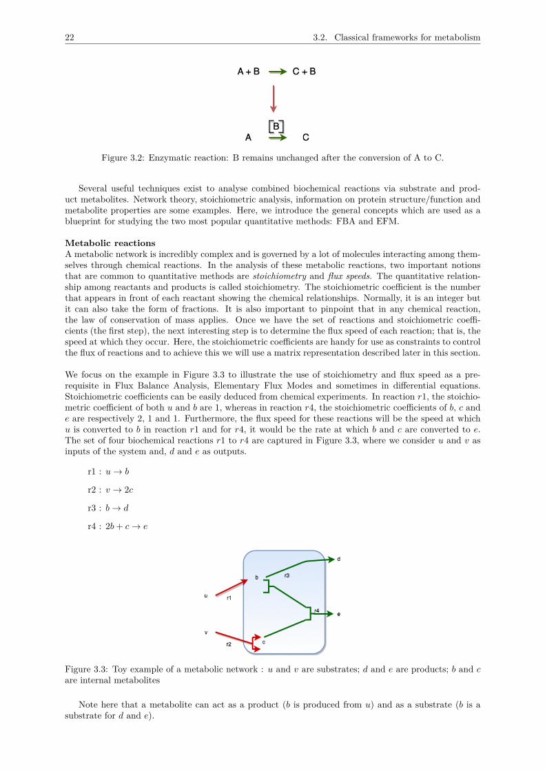
22 3.2. Classical frameworks for metabolism
Figure 3.2: Enzymatic reaction: B remains unchanged after the conversion of A to C.
Several useful techniques exist to analyse combined biochemical reactions via substrate and prod-uct metabolites. Network theory, stoichiometric analysis, information on protein structure/function andmetabolite properties are some examples. Here, we introduce the general concepts which are used as ablueprint for studying the two most popular quantitative methods: FBA and EFM.
Metabolic reactionsA metabolic network is incredibly complex and is governed by a lot of molecules interacting among them-selves through chemical reactions. In the analysis of these metabolic reactions, two important notionsthat are common to quantitative methods are stoichiometry and flux speeds. The quantitative relation-ship among reactants and products is called stoichiometry. The stoichiometric coefficient is the numberthat appears in front of each reactant showing the chemical relationships. Normally, it is an integer butit can also take the form of fractions. It is also important to pinpoint that in any chemical reaction,the law of conservation of mass applies. Once we have the set of reactions and stoichiometric coeffi-cients (the first step), the next interesting step is to determine the flux speed of each reaction; that is, thespeed at which they occur. Here, the stoichiometric coefficients are handy for use as constraints to controlthe flux of reactions and to achieve this we will use a matrix representation described later in this section.
We focus on the example in Figure 3.3 to illustrate the use of stoichiometry and flux speed as a pre-requisite in Flux Balance Analysis, Elementary Flux Modes and sometimes in differential equations.Stoichiometric coefficients can be easily deduced from chemical experiments. In reaction r1, the stoichio-metric coefficient of both u and b are 1, whereas in reaction r4, the stoichiometric coefficients of b, c ande are respectively 2, 1 and 1. Furthermore, the flux speed for these reactions will be the speed at whichu is converted to b in reaction r1 and for r4, it would be the rate at which b and c are converted to e.The set of four biochemical reactions r1 to r4 are captured in Figure 3.3, where we consider u and v asinputs of the system and, d and e as outputs.
r1 : u→ b
r2 : v → 2c
r3 : b→ d
r4 : 2b+ c→ e
Figure 3.3: Toy example of a metabolic network : u and v are substrates; d and e are products; b and care internal metabolites
Note here that a metabolite can act as a product (b is produced from u) and as a substrate (b is asubstrate for d and e).
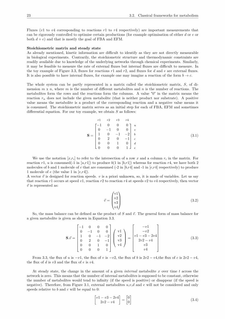
23 3.2. Classical frameworks for metabolism
Fluxes (v1 to v4 corresponding to reactions r1 to r4 respectively) are important measurements thatcan be rigorously controlled to optimise certain productions (for example optimisation of either d or e orboth d+ e) and that is mostly the goal of FBA and EFM.
Stoichiometric matrix and steady stateAs already mentioned, kinetic information are difficult to identify as they are not directly measurablein biological experiments. Contrarily, the stoichiometric structure and thermodynamic constraints arereadily available due to knowledge of the underlying networks through chemical experiments. Similarly,it may be feasible to measure the rate of external fluxes but internal fluxes are difficult to measure. Inthe toy example of Figure 3.3, fluxes for reactions r1 and r2, and fluxes for d and e are external fluxes.It is also possible to have internal fluxes, for example one may imagine a reaction of the form b→ c.
The whole system can be partly represented in a matrix called the stoichiometric matrix, S, of di-mension m x n, where m is the number of different metabolites and n is the number of reactions. Themetabolites form the rows and the reactions form the columns. A value "0" in the matrix means thereaction rn does not include the given metabolite (that is neither product nor substrate). A positivevalue means the metabolite is a product of the corresponding reaction and a negative value means itis consumed. The stoichiometric matrix serves as an initial step for each of FBA, EFM and sometimesdifferential equation. For our toy example, we obtain S as follows:
S =
r1 r2 r3 r4
−1 0 0 0 u
0 −1 0 0 v
1 0 −1 −2 b
0 2 0 −1 c
0 0 1 0 d
0 0 0 1 e
(3.1)
We use the notation [x,ri] to refer to the intersection of a row x and a column ri in the matrix. Forreaction r1, u is consumed(-1 in [u,r1]) to produce b(1 in [b,r1]) whereas for reaction r4, we have both 2molecules of b and 1 molecule of c that are consumed (-2 in [b,r4] and -1 in [c,r4] respectively) to produce1 molecule of e (the value 1 in [e,r4]).A vector ~v is designed for reaction speeds. v is a priori unknown, so, it is made of variables. Let us saythat reaction r1 occurs at speed v1, reaction r2 to reaction r4 at speeds v2 to v4 respectively, then vector~v is represented as:
~v =
v1v2v3v4
(3.2)
So, the mass balance can be defined as the product of S and ~v. The general form of mass balance fora given metabolite is given as shown in Equation 3.3.
S.~v =
−1 0 0 00 −1 0 01 0 −1 −20 2 0 −10 0 1 00 0 0 1
v1v2v3v4
=
−v1−v2
v1− v3− 2v42v2− v4
v3v4
(3.3)
From 3.3, the flux of u is −v1, the flux of v is −v2, the flux of b is 2v2− v4,the flux of c is 2v2− v4,the flux of d is v3 and the flux of e is v4.
At steady state, the change in the amount of a given internal metabolite x over time t across thenetwork is zero. This means that the number of internal metabolites is supposed to be constant, otherwisethe number of metabolites would tend to infinity (if the speed is positive) or disappear (if the speed isnegative). Therefore, from Figure 3.1, external metabolites u,v,d and e will not be considered and onlyspeeds relative to b and c will be equal to 0:[
v1− v3− 2v42v2− v4
]=[00
](3.4)
24 3.2. Classical frameworks for metabolism
From the stoichiometric matrix, by using S.~v=0 on internal metabolites, we impose certain constraintson ~v and at the same time, the fluxes are also interdependent. The "rest" of this vector of fluxes ~v canbe tuned for the optimisation of certain products.In our example, the list of internal metabolites are only b and c, from 3.4, this gives v1− v3− 2v4=0 and2v2− v4 = 0. And finally, this will end with v1 = v3 + 2v4 and v2 = 0.5v4, with only v3 and v4 left asunknowns. Thus, v3 and v4 "drive" the behaviour of external metabolites via the vector shown in 3.5,generating equations shown in 3.6:
−v3− 2v4 u−0.5v4 vv3 dv4 e
(3.5)
v4 = 2v2v3 = v1− 4v2 (3.6)
While these two basic steps are shared in quantitative metabolic analysis, the other remaining stepswill be different for FBA and EFM.
The next section continues with FBA to demonstrate how constraints are incorporated on these reactionsbased on biological knowledge of the studied metabolic network.
3.2.2 Flux Balance AnalysisIntroductionFlux balance analysis (FBA) has emerged as an effective modelling framework to analyse metabolic net-works in a quantitative manner [54] with a large repertoire of rigorous applications [55, 56, 57].
Five steps are involved in FBA metabolic reconstructions and analysis:
1. construction of the biochemical reactions for the system in question
2. linking the sets of enzymatic reactions with metabolites in a stoichiometry matrix and using it oninternal metabolites which are neither produced nor consumed (steady state condition)
3. using biological knowledge to extract minimum and maximum flux speeds of reactions
4. determining the objective function that is supposed to be optimized by the cell
5. identify the parameters in order to optimise the objective function
The first two preliminary steps of FBA have been elaborated in the previous section. We continue withthe same toy example to illustrate the next two steps of FBA. More often, there are normally more re-actions than the number of internal metabolites in a given model. Consequently, there remain unknownreactions speeds after the second step which results in a large number of solutions. When mass balanceconstraints imposed by the stoichiometric matrix S, and capacity constraints imposed by the lower andupper bounds are applied to a network, it defines an allowable solution space. With no additional con-straints, the flux distribution of a biological network may lie at any point in a solution space. To get amore accurate set of solutions, FBA introduces certain constraints. There exists two types of capacityconstraints : non-negativity constraints which reflect non-reversibility of reactions and main constraintswhich reflect maximal possible reactions speeds.
In our toy example, the constraints, v1 ≥ 0, v2 ≥ 0, v3 ≥ 0 and v4 ≥ 0 are non-negativity con-straints. If a reaction is non-reversible, then the minimum and maximum flux speeds for that reactionis always positive. In our toy network, we can, for example, have the following inequalities for the fourfluxes: 0 ≤ v1 ≤ 20, 0 ≤ v2 ≤ 7, 0 ≤ v3 ≤ 8 and 0 ≤ v4 ≤ 7.
Within the solution space, many possibilities are available. However, depending on the cellular pres-sures (cofactors, metabolites, gene regulations, environment, etc), the network will usually manifest itselfon a given phenotype (or a set of phenotypes). This means that the network (and the cell) will try to gotowards an "optimal solution" to achieve this phenotypic transition. For many metabolic networks, we
25 3.2. Classical frameworks for metabolism
can imagine, for example, optimal production of biomass or energy production. In mathematical terms,the modeller will create an objective function which is biologically relevant and optimise this function(maximise or minimise).
With respect to unknown variables, the set of linear inequalities and their constraints give rise to apolyhedral. FBA tries to identify the optimal points within this constrained space. Normally, the opti-mal solution is located in one of the corner of the polyhedral. To achieve this, FBA expresses the objectivefunction as Z = cT .v, where c is a vector of weights, indicating how much each reaction contributes tothe objective function. In practice, when only one reaction is desired for maximization or minimization,c is a vector of zeros with a one at the position of the reaction of interest. For example, if we want tooptimise the production of e, then we put a weight of 1 on reaction r4 and a weight of 0 on reactions r1,r2 and r3. In this case, the vector will be ~c = (0001). Suppose we want to optimise the production of etwice to that of d, then the vector ~c will be (0 0 1 2), and so on.
To solve this optimisation problem and find the right flux distribution, FBA uses linear programming.Since our toy example is a small network, it is easy to solve the two optimisation functions as follows:
• if ~c= (0 0 0 1), then we want to maximise v4 = 2v2; that is maximise v2 as well. Nevertheless,v2 cannot attain its maximum of 7 as we also need to have v4=2v2 ≤ 7. So, v2=3.5 and v1=7 isthe maximum. Moreover, v3 ≥ 0 and therefore v1 ≥ 4v2 = 14 which means 14 ≤ v1 ≤ 20. Mostprobably, one would choose the strict minimum value of v1=14, as a greater value of v1 wouldconsume u and produce d uselessly.
• if ~c= (0 0 1 2), then we want to maximise v3 + 2v4 = v1-4v2 +4v2; that is, we have to maximisev1. So, we choose the maximal value of v1=20. Moreover, we must choose v2 in such a way that v3≤ 8 because v3 = v1 - 4v2. Lastly, v4 must be less than or equal to 7, thus 3 ≤ v2 ≤ 3.5 becausev4 = 2v2. Most probably, one would choose the strict minimum value of v2=3, as a greater valueof v2 would consume v uselessly.
ToolsConstraint-based models, particularly those using FBA, have enabled the analysis of several large sys-tems, including entire (GSMNs) for prokaryotes [58], eukaryotes and human [40, 43], with a wide rangeof applications from metabolic engineering [56, 57] to drug discovery. Many simulation and visualisa-tion tools are used in the research community for in-silico FBA analysis. These include algorithms fromMOMA (minimisation of metabolic adjustment) and ROOM (regulatory on-off minimisation), and morepowerful network design tools like CellNetAnalyser (CNA) and COBRA.
DiscussionA wide spectrum of objective functions for analysis, with increasing biological relevance, are used toenable various types of predictions on the capabilities of metabolic networks. There have been interestingadvances in the area of FBA, with the integration of regulatory information as well as signalling networksinto the metabolic models. FBA has some remarkable advantages which are as follows:
• It is a fast metabolic framework as it relies only on three information on the network: stoichiometryof metabolites, metabolic demands and some few flux parameters. Since, there is no need forkinetic parameters (except for the determination of maximal speeds), FBA is computationally cheapeven in large networks. This stimulates model-driven discoveries by introducing a large number ofperturbations.
• Interestingly, reverse engineering can also be performed using FBA by extracting information fromlarge genome-scale experiments. Predicting, for example, gene knockouts to produce a biotechno-logical viable product.
• Additionally, FBA can help identify the knowledge gap presents in genomic data; that is reactionsthat are missing can be systematically identified by comparing in silico growth simulations toexperimental results [59].
However, the simplicity of FBA has the following drawbacks:
• The lack of kinetic parameters means FBA cannot predict metabolite concentrations and theirvariations in time, oscillations and so on. Furthermore, this also means that FBA cannot take intoaccount the dynamic behaviour of the model over time.
26 3.2. Classical frameworks for metabolism
• It is also only capable of determining fluxes at steady state for a particular objective function.But, the temporal evolution of the cell forces it not to optimise a certain metabolite infinitely. Forexample, the cell will not always optimise the growth of cells as it has other objectives like productionof energy to sustain other activities. These successive cell choices are of course regulated by higherlevel regulatory networks.
• A major challenge is often to find the definition of a biologically relevant objective function innetworks where there is a regulatory loop. Finally, FBA does not account for regulatory effectssuch as activation of enzymes by protein kinases or regulation of gene expression, so it lacks a degreeof accuracy in its predictions.
As a small reminder, our objective is to formulate the regulation of the metabolic network at thecoarse-grained level to understand causalities of metabolic processes. A shift from this coarse-grainedlevel to go down at metabolic levels would mean a shift from our objective. The dependency of FBAon metabolites would mean the analysis of too many biochemical reactions. The metabolic network ishighly regulated and is driven by a large number of regulatory loops with sophisticated feedbacks, whichcannot be handled by FBA tools. Our research focuses on the successive changes of the metabolic stateof the cell with a particular attention to biomass and energy. Using FBA will explicitly demand the listof all enzymatic reactions which amounts to hundreds and this is righteously not our main objective.Reasonably, to achieve this vision, we will therefore require a higher granular modelling. In conclusion,we will put aside FBA as a metabolic engineering tool, not suitable for the question we want to addressin this thesis.
Next, we will see a variant and a complement of FBA called Elementary Flux Modes (EFM), whichis a promising tool for pathway analysis and metabolic engineering.
3.2.3 Elementary Flux ModesIntroductionWhile FBA proposes only an optimal solution (single flux distribution) for a given metabolic network,a variant has been proposed by Schuster et al. [84, 85] called Elementary Flux Modes (EFM). Thismetabolic framework shares the same mathematical principle (first steps) with FBA; that is, firstly,constructing the network with an initial set of reactions (both reversible and irreversible) for both internaland external metabolites, and secondly building the stoichiometric matrix by aligning the reactionswith the metabolites. However, EFM introduces a systematic way of extracting biologically meaningfulpathways from an intricate metabolic network. These pathways (called elementary modes abbreviated asEM) consist of a minimal set of input metabolites and a minimal set of outputs. Compared to FBA, EFMdoes not require knowledge of any fixed flux rate and does not use any objective function. In general, aset of properties must be verified to generate EMs. They are as follows :
1. S. ~v = ~0 for internal metabolites (for steady state).
2. all reactions must be directed (proceeding in one direction will ensure positive flux values). Whena reaction is reversible, EFM simply asks to decompose it into two directed reactions for eachdirection.
3. the first two properties admit an infinite set of solutions. This additional constraint allows EFM togenerate finite sets of solutions.
4. in the attempt of optimising the outputs, we must have sufficiently EMs so that we can generateall the linear combinations of EMs with coeff ≥ 0.
The decomposition into elementary flux modes of a given metabolic network is not unique. It depends,for example, on the order of removal of non-linearly independent flux modes. To illustrate the proceduresinvolved in EFM, let us use the following set of reactions (captured in Figure 3.4 left), where r4/r5 andr6/r7 denote in fact two reversible reactions.
r1 : a→ b
r2 : b→ c
r3 : b→ d
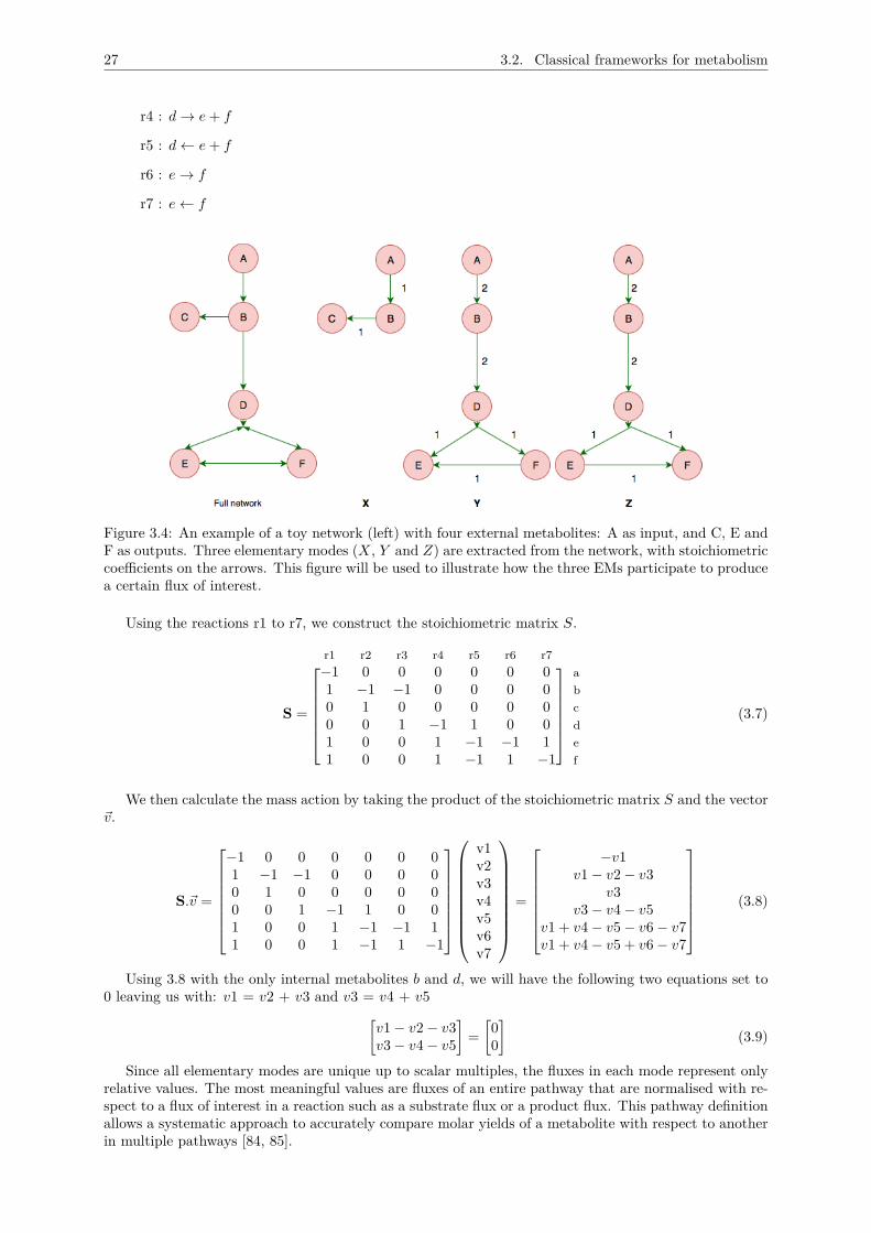
27 3.2. Classical frameworks for metabolism
r4 : d→ e+ f
r5 : d← e+ f
r6 : e→ f
r7 : e← f
Figure 3.4: An example of a toy network (left) with four external metabolites: A as input, and C, E andF as outputs. Three elementary modes (X, Y and Z) are extracted from the network, with stoichiometriccoefficients on the arrows. This figure will be used to illustrate how the three EMs participate to producea certain flux of interest.
Using the reactions r1 to r7, we construct the stoichiometric matrix S.
S =
r1 r2 r3 r4 r5 r6 r7
−1 0 0 0 0 0 0 a1 −1 −1 0 0 0 0 b0 1 0 0 0 0 0 c0 0 1 −1 1 0 0 d1 0 0 1 −1 −1 1 e1 0 0 1 −1 1 −1 f
(3.7)
We then calculate the mass action by taking the product of the stoichiometric matrix S and the vector~v.
S.~v =
−1 0 0 0 0 0 01 −1 −1 0 0 0 00 1 0 0 0 0 00 0 1 −1 1 0 01 0 0 1 −1 −1 11 0 0 1 −1 1 −1
v1v2v3v4v5v6v7
=
−v1
v1− v2− v3v3
v3− v4− v5v1 + v4− v5− v6− v7v1 + v4− v5 + v6− v7
(3.8)
Using 3.8 with the only internal metabolites b and d, we will have the following two equations set to0 leaving us with: v1 = v2 + v3 and v3 = v4 + v5[
v1− v2− v3v3− v4− v5
]=[00
](3.9)
Since all elementary modes are unique up to scalar multiples, the fluxes in each mode represent onlyrelative values. The most meaningful values are fluxes of an entire pathway that are normalised with re-spect to a flux of interest in a reaction such as a substrate flux or a product flux. This pathway definitionallows a systematic approach to accurately compare molar yields of a metabolite with respect to anotherin multiple pathways [84, 85].
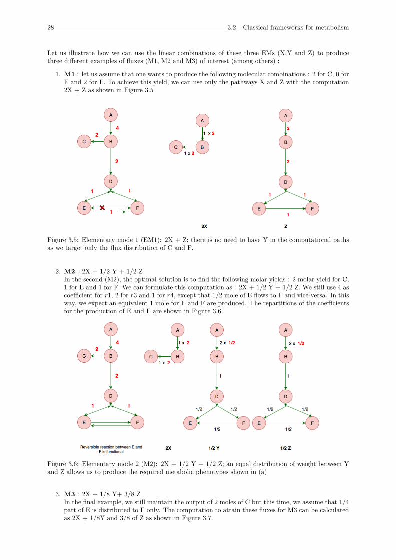
28 3.2. Classical frameworks for metabolism
Let us illustrate how we can use the linear combinations of these three EMs (X,Y and Z) to producethree different examples of fluxes (M1, M2 and M3) of interest (among others) :
1. M1 : let us assume that one wants to produce the following molecular combinations : 2 for C, 0 forE and 2 for F. To achieve this yield, we can use only the pathways X and Z with the computation2X + Z as shown in Figure 3.5
Figure 3.5: Elementary mode 1 (EM1): 2X + Z; there is no need to have Y in the computational pathsas we target only the flux distribution of C and F.
2. M2 : 2X + 1/2 Y + 1/2 ZIn the second (M2), the optimal solution is to find the following molar yields : 2 molar yield for C,1 for E and 1 for F. We can formulate this computation as : 2X + 1/2 Y + 1/2 Z. We still use 4 ascoefficient for r1, 2 for r3 and 1 for r4, except that 1/2 mole of E flows to F and vice-versa. In thisway, we expect an equivalent 1 mole for E and F are produced. The repartitions of the coefficientsfor the production of E and F are shown in Figure 3.6.
Figure 3.6: Elementary mode 2 (M2): 2X + 1/2 Y + 1/2 Z; an equal distribution of weight between Yand Z allows us to produce the required metabolic phenotypes shown in (a)
3. M3 : 2X + 1/8 Y+ 3/8 ZIn the final example, we still maintain the output of 2 moles of C but this time, we assume that 1/4part of E is distributed to F only. The computation to attain these fluxes for M3 can be calculatedas 2X + 1/8Y and 3/8 of Z as shown in Figure 3.7.
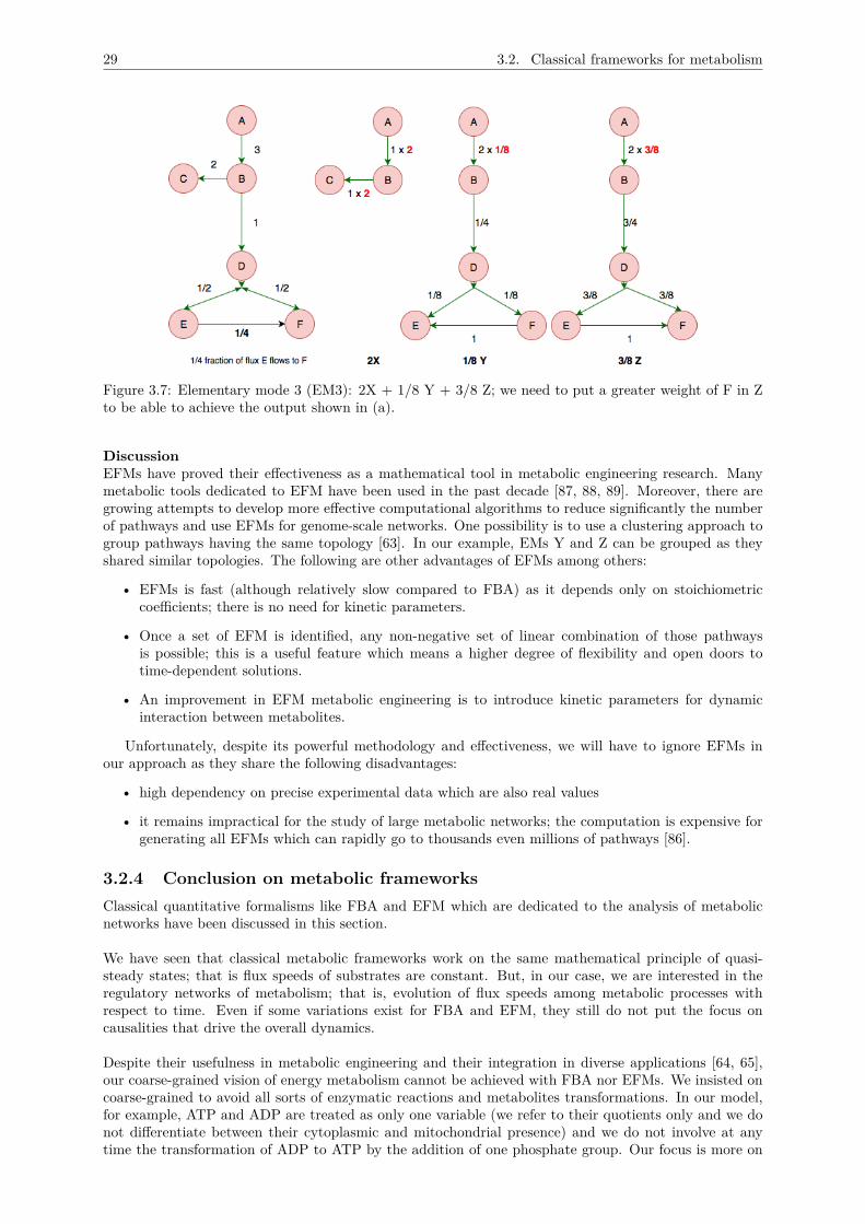
29 3.2. Classical frameworks for metabolism
Figure 3.7: Elementary mode 3 (EM3): 2X + 1/8 Y + 3/8 Z; we need to put a greater weight of F in Zto be able to achieve the output shown in (a).
DiscussionEFMs have proved their effectiveness as a mathematical tool in metabolic engineering research. Manymetabolic tools dedicated to EFM have been used in the past decade [87, 88, 89]. Moreover, there aregrowing attempts to develop more effective computational algorithms to reduce significantly the numberof pathways and use EFMs for genome-scale networks. One possibility is to use a clustering approach togroup pathways having the same topology [63]. In our example, EMs Y and Z can be grouped as theyshared similar topologies. The following are other advantages of EFMs among others:
• EFMs is fast (although relatively slow compared to FBA) as it depends only on stoichiometriccoefficients; there is no need for kinetic parameters.
• Once a set of EFM is identified, any non-negative set of linear combination of those pathwaysis possible; this is a useful feature which means a higher degree of flexibility and open doors totime-dependent solutions.
• An improvement in EFM metabolic engineering is to introduce kinetic parameters for dynamicinteraction between metabolites.
Unfortunately, despite its powerful methodology and effectiveness, we will have to ignore EFMs inour approach as they share the following disadvantages:
• high dependency on precise experimental data which are also real values
• it remains impractical for the study of large metabolic networks; the computation is expensive forgenerating all EFMs which can rapidly go to thousands even millions of pathways [86].
3.2.4 Conclusion on metabolic frameworksClassical quantitative formalisms like FBA and EFM which are dedicated to the analysis of metabolicnetworks have been discussed in this section.
We have seen that classical metabolic frameworks work on the same mathematical principle of quasi-steady states; that is flux speeds of substrates are constant. But, in our case, we are interested in theregulatory networks of metabolism; that is, evolution of flux speeds among metabolic processes withrespect to time. Even if some variations exist for FBA and EFM, they still do not put the focus oncausalities that drive the overall dynamics.
Despite their usefulness in metabolic engineering and their integration in diverse applications [64, 65],our coarse-grained vision of energy metabolism cannot be achieved with FBA nor EFMs. We insisted oncoarse-grained to avoid all sorts of enzymatic reactions and metabolites transformations. In our model,for example, ATP and ADP are treated as only one variable (we refer to their quotients only and we donot differentiate between their cytoplasmic and mitochondrial presence) and we do not involve at anytime the transformation of ADP to ATP by the addition of one phosphate group. Our focus is more on
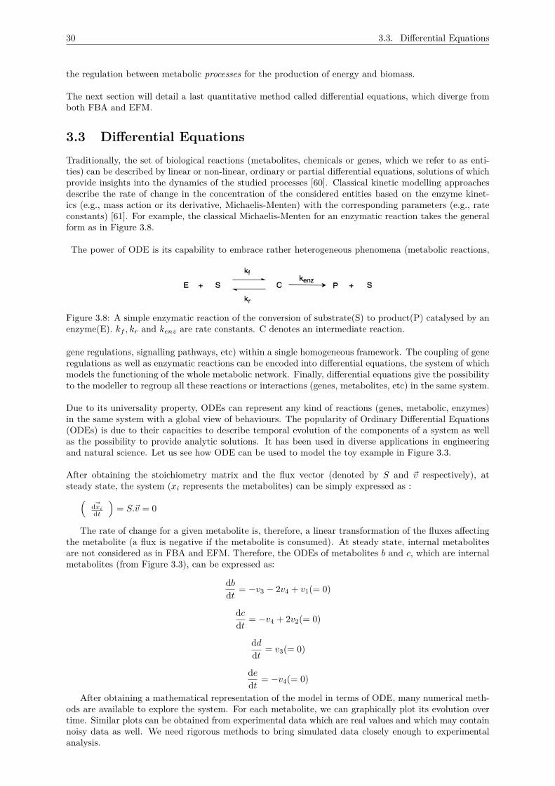
30 3.3. Differential Equations
the regulation between metabolic processes for the production of energy and biomass.
The next section will detail a last quantitative method called differential equations, which diverge fromboth FBA and EFM.
3.3 Differential EquationsTraditionally, the set of biological reactions (metabolites, chemicals or genes, which we refer to as enti-ties) can be described by linear or non-linear, ordinary or partial differential equations, solutions of whichprovide insights into the dynamics of the studied processes [60]. Classical kinetic modelling approachesdescribe the rate of change in the concentration of the considered entities based on the enzyme kinet-ics (e.g., mass action or its derivative, Michaelis-Menten) with the corresponding parameters (e.g., rateconstants) [61]. For example, the classical Michaelis-Menten for an enzymatic reaction takes the generalform as in Figure 3.8.
The power of ODE is its capability to embrace rather heterogeneous phenomena (metabolic reactions,
Figure 3.8: A simple enzymatic reaction of the conversion of substrate(S) to product(P) catalysed by anenzyme(E). kf , kr and kenz are rate constants. C denotes an intermediate reaction.
gene regulations, signalling pathways, etc) within a single homogeneous framework. The coupling of generegulations as well as enzymatic reactions can be encoded into differential equations, the system of whichmodels the functioning of the whole metabolic network. Finally, differential equations give the possibilityto the modeller to regroup all these reactions or interactions (genes, metabolites, etc) in the same system.
Due to its universality property, ODEs can represent any kind of reactions (genes, metabolic, enzymes)in the same system with a global view of behaviours. The popularity of Ordinary Differential Equations(ODEs) is due to their capacities to describe temporal evolution of the components of a system as wellas the possibility to provide analytic solutions. It has been used in diverse applications in engineeringand natural science. Let us see how ODE can be used to model the toy example in Figure 3.3.
After obtaining the stoichiometry matrix and the flux vector (denoted by S and ~v respectively), atsteady state, the system (xi represents the metabolites) can be simply expressed as :(
~dxi
dt
)= S.~v = 0
The rate of change for a given metabolite is, therefore, a linear transformation of the fluxes affectingthe metabolite (a flux is negative if the metabolite is consumed). At steady state, internal metabolitesare not considered as in FBA and EFM. Therefore, the ODEs of metabolites b and c, which are internalmetabolites (from Figure 3.3), can be expressed as:
dbdt = −v3 − 2v4 + v1(= 0)
dcdt = −v4 + 2v2(= 0)
dddt = v3(= 0)
dedt = −v4(= 0)
After obtaining a mathematical representation of the model in terms of ODE, many numerical meth-ods are available to explore the system. For each metabolite, we can graphically plot its evolution overtime. Similar plots can be obtained from experimental data which are real values and which may containnoisy data as well. We need rigorous methods to bring simulated data closely enough to experimentalanalysis.
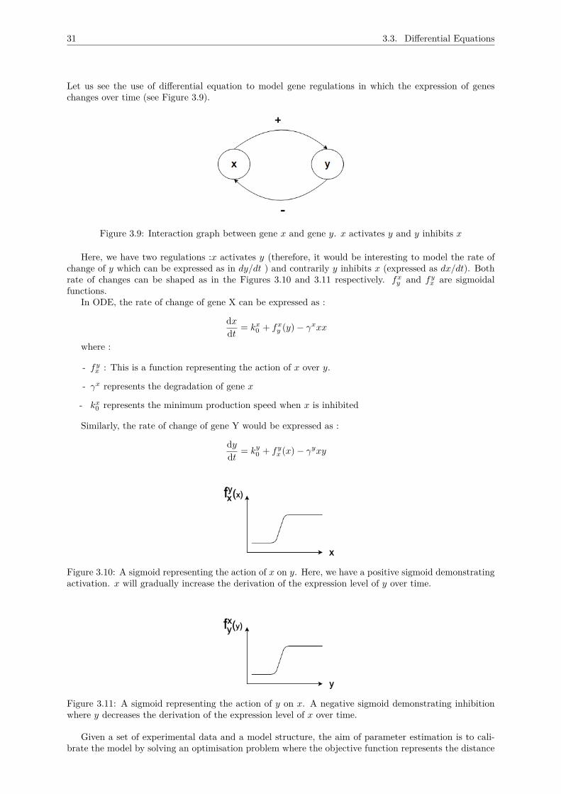
31 3.3. Differential Equations
Let us see the use of differential equation to model gene regulations in which the expression of geneschanges over time (see Figure 3.9).
Figure 3.9: Interaction graph between gene x and gene y. x activates y and y inhibits x
Here, we have two regulations :x activates y (therefore, it would be interesting to model the rate ofchange of y which can be expressed as in dy/dt ) and contrarily y inhibits x (expressed as dx/dt). Bothrate of changes can be shaped as in the Figures 3.10 and 3.11 respectively. fx
y and fyx are sigmoidal
functions.In ODE, the rate of change of gene X can be expressed as :
dxdt = kx
0 + fxy (y)− γxxx
where :
- fyx : This is a function representing the action of x over y.
- γx represents the degradation of gene x
- kx0 represents the minimum production speed when x is inhibited
Similarly, the rate of change of gene Y would be expressed as :
dydt = ky
0 + fyx (x)− γyxy
Figure 3.10: A sigmoid representing the action of x on y. Here, we have a positive sigmoid demonstratingactivation. x will gradually increase the derivation of the expression level of y over time.
Figure 3.11: A sigmoid representing the action of y on x. A negative sigmoid demonstrating inhibitionwhere y decreases the derivation of the expression level of x over time.
Given a set of experimental data and a model structure, the aim of parameter estimation is to cali-brate the model by solving an optimisation problem where the objective function represents the distance
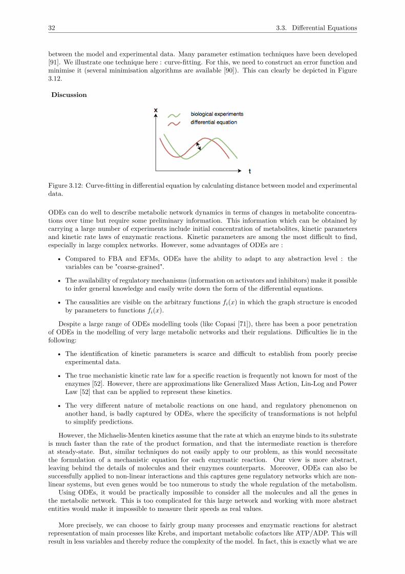
32 3.3. Differential Equations
between the model and experimental data. Many parameter estimation techniques have been developed[91]. We illustrate one technique here : curve-fitting. For this, we need to construct an error function andminimise it (several minimisation algorithms are available [90]). This can clearly be depicted in Figure3.12.
Discussion
Figure 3.12: Curve-fitting in differential equation by calculating distance between model and experimentaldata.
ODEs can do well to describe metabolic network dynamics in terms of changes in metabolite concentra-tions over time but require some preliminary information. This information which can be obtained bycarrying a large number of experiments include initial concentration of metabolites, kinetic parametersand kinetic rate laws of enzymatic reactions. Kinetic parameters are among the most difficult to find,especially in large complex networks. However, some advantages of ODEs are :
• Compared to FBA and EFMs, ODEs have the ability to adapt to any abstraction level : thevariables can be "coarse-grained".
• The availability of regulatory mechanisms (information on activators and inhibitors) make it possibleto infer general knowledge and easily write down the form of the differential equations.
• The causalities are visible on the arbitrary functions fi(x) in which the graph structure is encodedby parameters to functions fi(x).
Despite a large range of ODEs modelling tools (like Copasi [71]), there has been a poor penetrationof ODEs in the modelling of very large metabolic networks and their regulations. Difficulties lie in thefollowing:
• The identification of kinetic parameters is scarce and difficult to establish from poorly preciseexperimental data.
• The true mechanistic kinetic rate law for a specific reaction is frequently not known for most of theenzymes [52]. However, there are approximations like Generalized Mass Action, Lin-Log and PowerLaw [52] that can be applied to represent these kinetics.
• The very different nature of metabolic reactions on one hand, and regulatory phenomenon onanother hand, is badly captured by ODEs, where the specificity of transformations is not helpfulto simplify predictions.
However, the Michaelis-Menten kinetics assume that the rate at which an enzyme binds to its substrateis much faster than the rate of the product formation, and that the intermediate reaction is thereforeat steady-state. But, similar techniques do not easily apply to our problem, as this would necessitatethe formulation of a mechanistic equation for each enzymatic reaction. Our view is more abstract,leaving behind the details of molecules and their enzymes counterparts. Moreover, ODEs can also besuccessfully applied to non-linear interactions and this captures gene regulatory networks which are non-linear systems, but even genes would be too numerous to study the whole regulation of the metabolism.
Using ODEs, it would be practically impossible to consider all the molecules and all the genes inthe metabolic network. This is too complicated for this large network and working with more abstractentities would make it impossible to measure their speeds as real values.
More precisely, we can choose to fairly group many processes and enzymatic reactions for abstractrepresentation of main processes like Krebs, and important metabolic cofactors like ATP/ADP. This willresult in less variables and thereby reduce the complexity of the model. In fact, this is exactly what we are
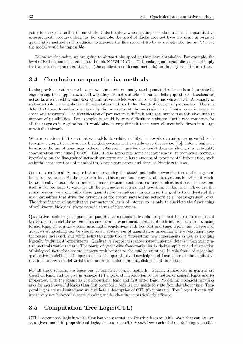
33 3.4. Conclusion on quantitative methods
going to carry out further in our study. Unfortunately, when making such abstractions, the quantitativemeasurements become unfeasible. For example, the speed of Krebs does not have any sense in terms ofquantitative method as it is difficult to measure the flux speed of Krebs as a whole. So, the validation ofthe model would be impossible.
Following this point, we are going to abstract the speed as they have thresholds. For example, thelevel of Krebs is sufficient enough to inhibit NADH/NAD+. This makes good metabolic sense and implythat we can do some discretisations (the application of formal methods) on these types of information.
3.4 Conclusion on quantitative methodsIn the previous sections, we have shown the most commonly used quantitative formalisms in metabolicengineering, their applications and why they are not suitable for our modelling questions. Biochemicalnetworks are incredibly complex. Quantitative models work more at the molecular level. A panoply ofsoftware tools is available both for simulation and partly for the identification of parameters. The soledefault of these formalisms is precisely the occurence at the molecular level (concurrency in terms ofspeed and resources). The identification of parameters is difficult with real numbers as this gives infinitenumber of possibilities. For example, it would be very difficult to estimate kinetic rate constants forall the enzymes in respiration. It would also be very difficult to measure all metabolic fluxes in a largemetabolic network.
We are conscious that quantitative models describing metabolic network dynamics are powerful toolsto explain properties of complex biological systems and to guide experimentation [75]. Interestingly, wehave seen the use of non-linear ordinary differential equations to model dynamic changes in metaboliteconcentration over time [76, 58]. But, it also represents some inconveniences: it requires a previousknowledge on the fine-grained network structure and a large amount of experimental information, suchas initial concentrations of metabolites, kinetic parameters and detailed kinetic rate laws.
Our research is mainly targeted at understanding the global metabolic network in terms of energy andbiomass production. At the molecular level, this means too many metabolic reactions for which it wouldbe practically impossible to perform precise measurements and parameter identifications. The systemitself is far too large to cater for all the enzymatic reactions and modelling at this level. These are theprime reasons we avoid using these quantitative formalisms. In our case, the goal is to understand themain causalities that drive the dynamics of the energy metabolism network at a "coarse-grained" level.The identification of quantitative parameter values is of interest to us only to elucidate the functioningof well-known biological phenomena in terms of phenotypes.
Qualitative modelling compared to quantitative methods is less data-dependent but requires sufficientknowledge to model the system. In some research experiments, data is of little interest because, by usingformal logic, we can draw some meaningful conclusions with less cost and time. From this perspective,qualitative modelling can be viewed as an abstraction of quantitative modelling where reasoning capa-bilities are increased, and which helps the prediction of "interesting" new experiments as well as avoidinglogically "redundant" experiments. Qualitative approaches ignore some numerical details which quantita-tive methods would require. The power of qualitative frameworks lies in their simplicity and abstractionof biological facts that are transparent with respect to the studied question. In this frame of reasoning,qualitative modelling techniques sacrifice the quantitative knowledge and focus more on the qualitativerelations between model variables in order to explore and establish general properties.
For all these reasons, we focus our attention to formal methods. Formal frameworks in general arebased on logic, and we give in Annexe 11.1 a general introduction to the notion of general logics and itsproperties, with the examples of propositional logic and first order logic. Modelling biological networksasks for more powerful logics than first order logic because one needs to state formulas about time. Tem-poral logics are well suited and we give here a description of CTL (Computation Tree Logic) that we willintensively use because its corresponding model checking is particularly efficient.
3.5 Computation Tree Logic(CTL)CTL is a temporal logic in which time has a tree structure. Starting from an initial state that can be seenas a given model in propositional logic, there are possible transitions, each of them defining a possible
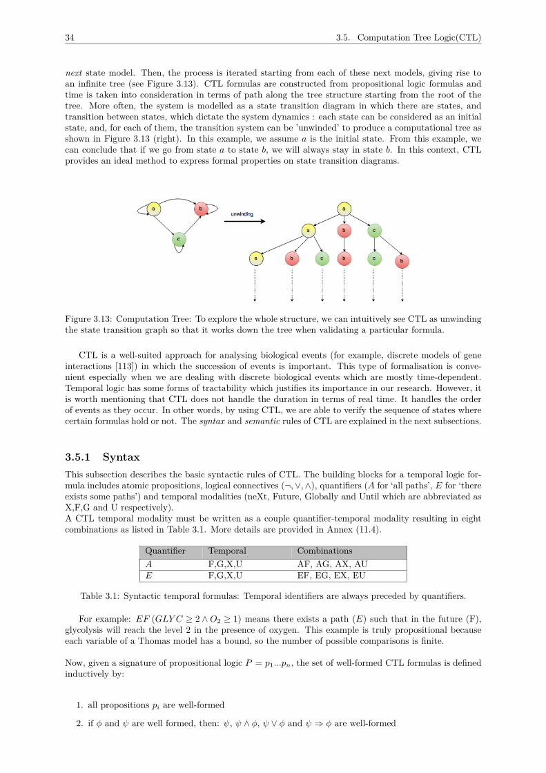
34 3.5. Computation Tree Logic(CTL)
next state model. Then, the process is iterated starting from each of these next models, giving rise toan infinite tree (see Figure 3.13). CTL formulas are constructed from propositional logic formulas andtime is taken into consideration in terms of path along the tree structure starting from the root of thetree. More often, the system is modelled as a state transition diagram in which there are states, andtransition between states, which dictate the system dynamics : each state can be considered as an initialstate, and, for each of them, the transition system can be ’unwinded’ to produce a computational tree asshown in Figure 3.13 (right). In this example, we assume a is the initial state. From this example, wecan conclude that if we go from state a to state b, we will always stay in state b. In this context, CTLprovides an ideal method to express formal properties on state transition diagrams.
Figure 3.13: Computation Tree: To explore the whole structure, we can intuitively see CTL as unwindingthe state transition graph so that it works down the tree when validating a particular formula.
CTL is a well-suited approach for analysing biological events (for example, discrete models of geneinteractions [113]) in which the succession of events is important. This type of formalisation is conve-nient especially when we are dealing with discrete biological events which are mostly time-dependent.Temporal logic has some forms of tractability which justifies its importance in our research. However, itis worth mentioning that CTL does not handle the duration in terms of real time. It handles the orderof events as they occur. In other words, by using CTL, we are able to verify the sequence of states wherecertain formulas hold or not. The syntax and semantic rules of CTL are explained in the next subsections.
3.5.1 SyntaxThis subsection describes the basic syntactic rules of CTL. The building blocks for a temporal logic for-mula includes atomic propositions, logical connectives (¬,∨,∧), quantifiers (A for ‘all paths’, E for ‘thereexists some paths’) and temporal modalities (neXt, Future, Globally and Until which are abbreviated asX,F,G and U respectively).A CTL temporal modality must be written as a couple quantifier-temporal modality resulting in eightcombinations as listed in Table 3.1. More details are provided in Annex (11.4).
Quantifier Temporal CombinationsA F,G,X,U AF, AG, AX, AUE F,G,X,U EF, EG, EX, EU
Table 3.1: Syntactic temporal formulas: Temporal identifiers are always preceded by quantifiers.
For example: EF (GLY C ≥ 2 ∧O2 ≥ 1) means there exists a path (E) such that in the future (F),glycolysis will reach the level 2 in the presence of oxygen. This example is truly propositional becauseeach variable of a Thomas model has a bound, so the number of possible comparisons is finite.
Now, given a signature of propositional logic P = p1...pn, the set of well-formed CTL formulas is definedinductively by:
1. all propositions pi are well-formed
2. if φ and ψ are well formed, then: ψ, ψ ∧ φ, ψ ∨ φ and ψ ⇒ φ are well-formed
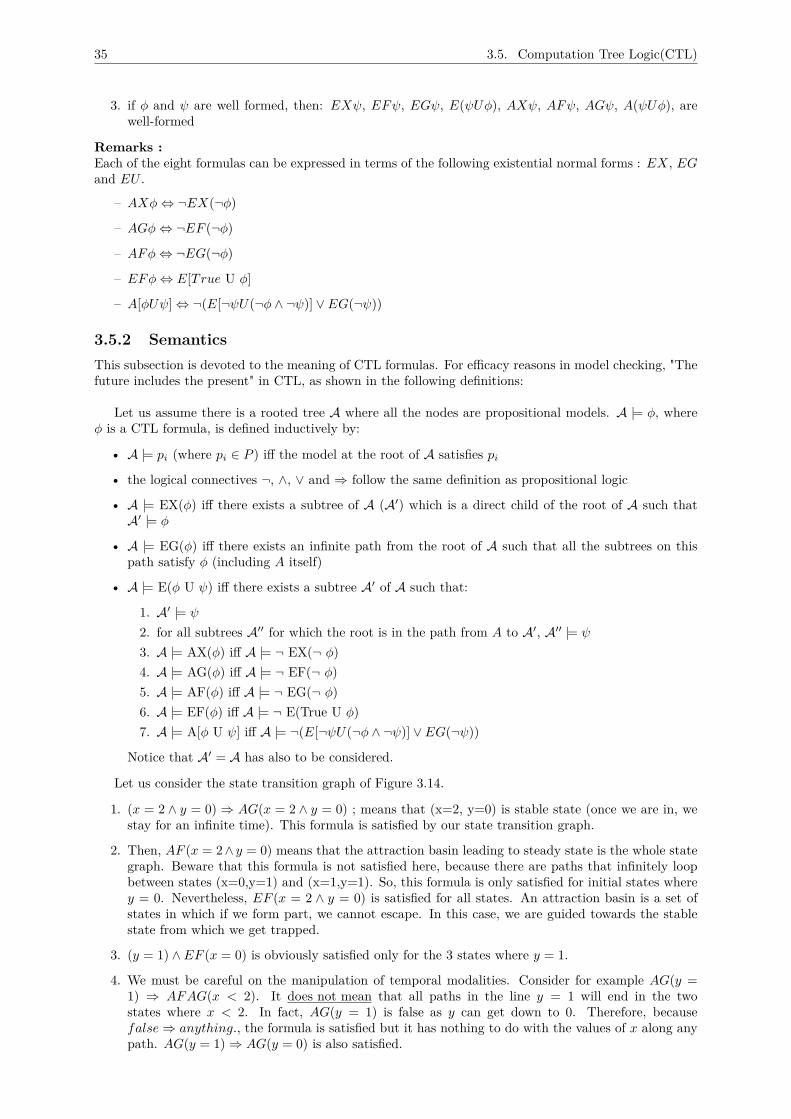
35 3.5. Computation Tree Logic(CTL)
3. if φ and ψ are well formed, then: EXψ, EFψ, EGψ, E(ψUφ), AXψ, AFψ, AGψ, A(ψUφ), arewell-formed
Remarks :Each of the eight formulas can be expressed in terms of the following existential normal forms : EX, EGand EU .
– AXφ⇔ ¬EX(¬φ)
– AGφ⇔ ¬EF (¬φ)
– AFφ⇔ ¬EG(¬φ)
– EFφ⇔ E[True U φ]
– A[φUψ]⇔ ¬(E[¬ψU(¬φ ∧ ¬ψ)] ∨ EG(¬ψ))
3.5.2 SemanticsThis subsection is devoted to the meaning of CTL formulas. For efficacy reasons in model checking, "Thefuture includes the present" in CTL, as shown in the following definitions:
Let us assume there is a rooted tree A where all the nodes are propositional models. A |= φ, whereφ is a CTL formula, is defined inductively by:
• A |= pi (where pi ∈ P ) iff the model at the root of A satisfies pi
• the logical connectives ¬, ∧, ∨ and ⇒ follow the same definition as propositional logic
• A |= EX(φ) iff there exists a subtree of A (A′) which is a direct child of the root of A such thatA′ |= φ
• A |= EG(φ) iff there exists an infinite path from the root of A such that all the subtrees on thispath satisfy φ (including A itself)
• A |= E(φ U ψ) iff there exists a subtree A′ of A such that:
1. A′ |= ψ
2. for all subtrees A′′ for which the root is in the path from A to A′, A′′ |= ψ
3. A |= AX(φ) iff A |= ¬ EX(¬ φ)4. A |= AG(φ) iff A |= ¬ EF(¬ φ)5. A |= AF(φ) iff A |= ¬ EG(¬ φ)6. A |= EF(φ) iff A |= ¬ E(True U φ)7. A |= A[φ U ψ] iff A |= ¬(E[¬ψU(¬φ ∧ ¬ψ)] ∨ EG(¬ψ))
Notice that A′ = A has also to be considered.
Let us consider the state transition graph of Figure 3.14.
1. (x = 2 ∧ y = 0)⇒ AG(x = 2 ∧ y = 0) ; means that (x=2, y=0) is stable state (once we are in, westay for an infinite time). This formula is satisfied by our state transition graph.
2. Then, AF (x = 2∧ y = 0) means that the attraction basin leading to steady state is the whole stategraph. Beware that this formula is not satisfied here, because there are paths that infinitely loopbetween states (x=0,y=1) and (x=1,y=1). So, this formula is only satisfied for initial states wherey = 0. Nevertheless, EF (x = 2 ∧ y = 0) is satisfied for all states. An attraction basin is a set ofstates in which if we form part, we cannot escape. In this case, we are guided towards the stablestate from which we get trapped.
3. (y = 1) ∧ EF (x = 0) is obviously satisfied only for the 3 states where y = 1.
4. We must be careful on the manipulation of temporal modalities. Consider for example AG(y =1) ⇒ AFAG(x < 2). It does not mean that all paths in the line y = 1 will end in the twostates where x < 2. In fact, AG(y = 1) is false as y can get down to 0. Therefore, becausefalse⇒ anything., the formula is satisfied but it has nothing to do with the values of x along anypath. AG(y = 1)⇒ AG(y = 0) is also satisfied.
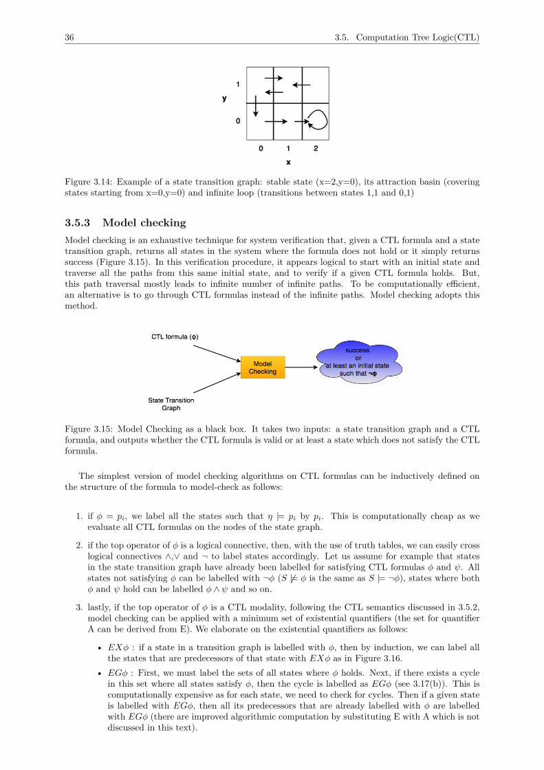
36 3.5. Computation Tree Logic(CTL)
Figure 3.14: Example of a state transition graph: stable state (x=2,y=0), its attraction basin (coveringstates starting from x=0,y=0) and infinite loop (transitions between states 1,1 and 0,1)
3.5.3 Model checkingModel checking is an exhaustive technique for system verification that, given a CTL formula and a statetransition graph, returns all states in the system where the formula does not hold or it simply returnssuccess (Figure 3.15). In this verification procedure, it appears logical to start with an initial state andtraverse all the paths from this same initial state, and to verify if a given CTL formula holds. But,this path traversal mostly leads to infinite number of infinite paths. To be computationally efficient,an alternative is to go through CTL formulas instead of the infinite paths. Model checking adopts thismethod.
Figure 3.15: Model Checking as a black box. It takes two inputs: a state transition graph and a CTLformula, and outputs whether the CTL formula is valid or at least a state which does not satisfy the CTLformula.
The simplest version of model checking algorithms on CTL formulas can be inductively defined onthe structure of the formula to model-check as follows:
1. if φ = pi, we label all the states such that η |= pi by pi. This is computationally cheap as weevaluate all CTL formulas on the nodes of the state graph.
2. if the top operator of φ is a logical connective, then, with the use of truth tables, we can easily crosslogical connectives ∧,∨ and ¬ to label states accordingly. Let us assume for example that statesin the state transition graph have already been labelled for satisfying CTL formulas φ and ψ. Allstates not satisfying φ can be labelled with ¬φ (S 6|= φ is the same as S |= ¬φ), states where bothφ and ψ hold can be labelled φ ∧ ψ and so on.
3. lastly, if the top operator of φ is a CTL modality, following the CTL semantics discussed in 3.5.2,model checking can be applied with a minimum set of existential quantifiers (the set for quantifierA can be derived from E). We elaborate on the existential quantifiers as follows:
• EXφ : if a state in a transition graph is labelled with φ, then by induction, we can label allthe states that are predecessors of that state with EXφ as in Figure 3.16.
• EGφ : First, we must label the sets of all states where φ holds. Next, if there exists a cyclein this set where all states satisfy φ, then the cycle is labelled as EGφ (see 3.17(b)). This iscomputationally expensive as for each state, we need to check for cycles. Then if a given stateis labelled with EGφ, then all its predecessors that are already labelled with φ are labelledwith EGφ (there are improved algorithmic computation by substituting E with A which is notdiscussed in this text).
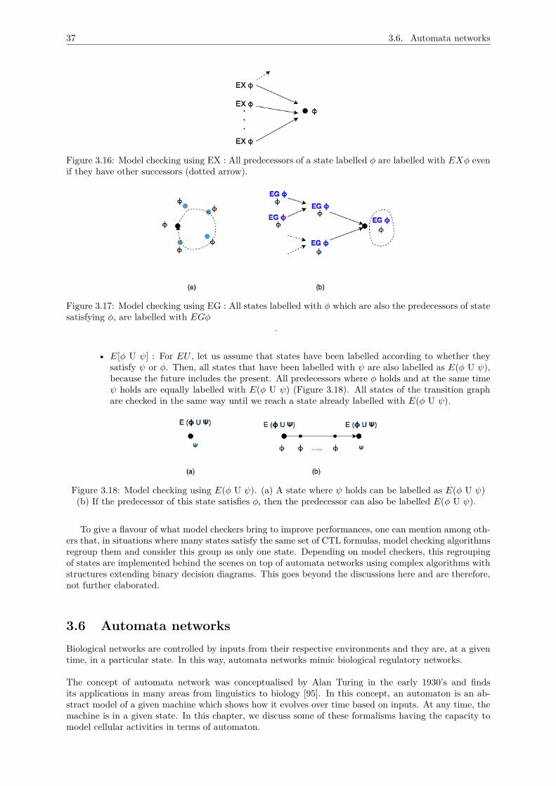
37 3.6. Automata networks
Figure 3.16: Model checking using EX : All predecessors of a state labelled φ are labelled with EXφ evenif they have other successors (dotted arrow).
Figure 3.17: Model checking using EG : All states labelled with φ which are also the predecessors of statesatisfying φ, are labelled with EGφ
.
• E[φ U ψ] : For EU , let us assume that states have been labelled according to whether theysatisfy ψ or φ. Then, all states that have been labelled with ψ are also labelled as E(φ U ψ),because the future includes the present. All predecessors where φ holds and at the same timeψ holds are equally labelled with E(φ U ψ) (Figure 3.18). All states of the transition graphare checked in the same way until we reach a state already labelled with E(φ U ψ).
Figure 3.18: Model checking using E(φ U ψ). (a) A state where ψ holds can be labelled as E(φ U ψ)(b) If the predecessor of this state satisfies φ, then the predecessor can also be labelled E(φ U ψ).
To give a flavour of what model checkers bring to improve performances, one can mention among oth-ers that, in situations where many states satisfy the same set of CTL formulas, model checking algorithmsregroup them and consider this group as only one state. Depending on model checkers, this regroupingof states are implemented behind the scenes on top of automata networks using complex algorithms withstructures extending binary decision diagrams. This goes beyond the discussions here and are therefore,not further elaborated.
3.6 Automata networksBiological networks are controlled by inputs from their respective environments and they are, at a giventime, in a particular state. In this way, automata networks mimic biological regulatory networks.
The concept of automata network was conceptualised by Alan Turing in the early 1930’s and findsits applications in many areas from linguistics to biology [95]. In this concept, an automaton is an ab-stract model of a given machine which shows how it evolves over time based on inputs. At any time, themachine is in a given state. In this chapter, we discuss some of these formalisms having the capacity tomodel cellular activities in terms of automaton.
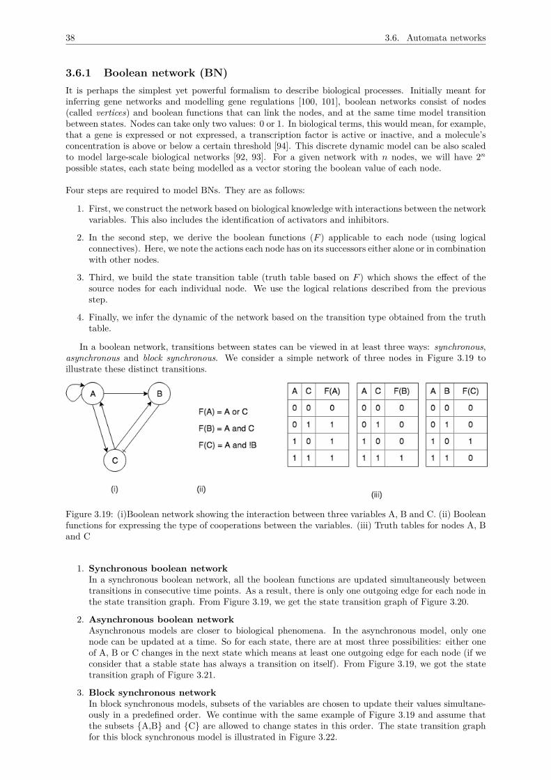
38 3.6. Automata networks
3.6.1 Boolean network (BN)It is perhaps the simplest yet powerful formalism to describe biological processes. Initially meant forinferring gene networks and modelling gene regulations [100, 101], boolean networks consist of nodes(called vertices) and boolean functions that can link the nodes, and at the same time model transitionbetween states. Nodes can take only two values: 0 or 1. In biological terms, this would mean, for example,that a gene is expressed or not expressed, a transcription factor is active or inactive, and a molecule’sconcentration is above or below a certain threshold [94]. This discrete dynamic model can be also scaledto model large-scale biological networks [92, 93]. For a given network with n nodes, we will have 2n
possible states, each state being modelled as a vector storing the boolean value of each node.
Four steps are required to model BNs. They are as follows:
1. First, we construct the network based on biological knowledge with interactions between the networkvariables. This also includes the identification of activators and inhibitors.
2. In the second step, we derive the boolean functions (F ) applicable to each node (using logicalconnectives). Here, we note the actions each node has on its successors either alone or in combinationwith other nodes.
3. Third, we build the state transition table (truth table based on F ) which shows the effect of thesource nodes for each individual node. We use the logical relations described from the previousstep.
4. Finally, we infer the dynamic of the network based on the transition type obtained from the truthtable.
In a boolean network, transitions between states can be viewed in at least three ways: synchronous,asynchronous and block synchronous. We consider a simple network of three nodes in Figure 3.19 toillustrate these distinct transitions.
Figure 3.19: (i)Boolean network showing the interaction between three variables A, B and C. (ii) Booleanfunctions for expressing the type of cooperations between the variables. (iii) Truth tables for nodes A, Band C
1. Synchronous boolean networkIn a synchronous boolean network, all the boolean functions are updated simultaneously betweentransitions in consecutive time points. As a result, there is only one outgoing edge for each node inthe state transition graph. From Figure 3.19, we get the state transition graph of Figure 3.20.
2. Asynchronous boolean networkAsynchronous models are closer to biological phenomena. In the asynchronous model, only onenode can be updated at a time. So for each state, there are at most three possibilities: either oneof A, B or C changes in the next state which means at least one outgoing edge for each node (if weconsider that a stable state has always a transition on itself). From Figure 3.19, we got the statetransition graph of Figure 3.21.
3. Block synchronous networkIn block synchronous models, subsets of the variables are chosen to update their values simultane-ously in a predefined order. We continue with the same example of Figure 3.19 and assume thatthe subsets {A,B} and {C} are allowed to change states in this order. The state transition graphfor this block synchronous model is illustrated in Figure 3.22.
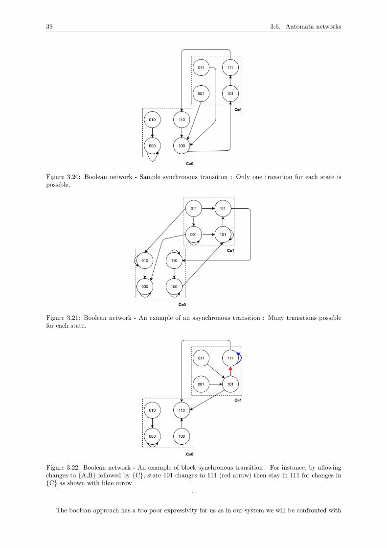
39 3.6. Automata networks
Figure 3.20: Boolean network - Sample synchronous transition : Only one transition for each state ispossible.
Figure 3.21: Boolean network - An example of an asynchronous transition : Many transitions possiblefor each state.
Figure 3.22: Boolean network - An example of block synchronous transition : For instance, by allowingchanges to {A,B} followed by {C}, state 101 changes to 111 (red arrow) then stay in 111 for changes in{C} as shown with blue arrow
.
The boolean approach has a too poor expressivity for us as in our system we will be confronted with
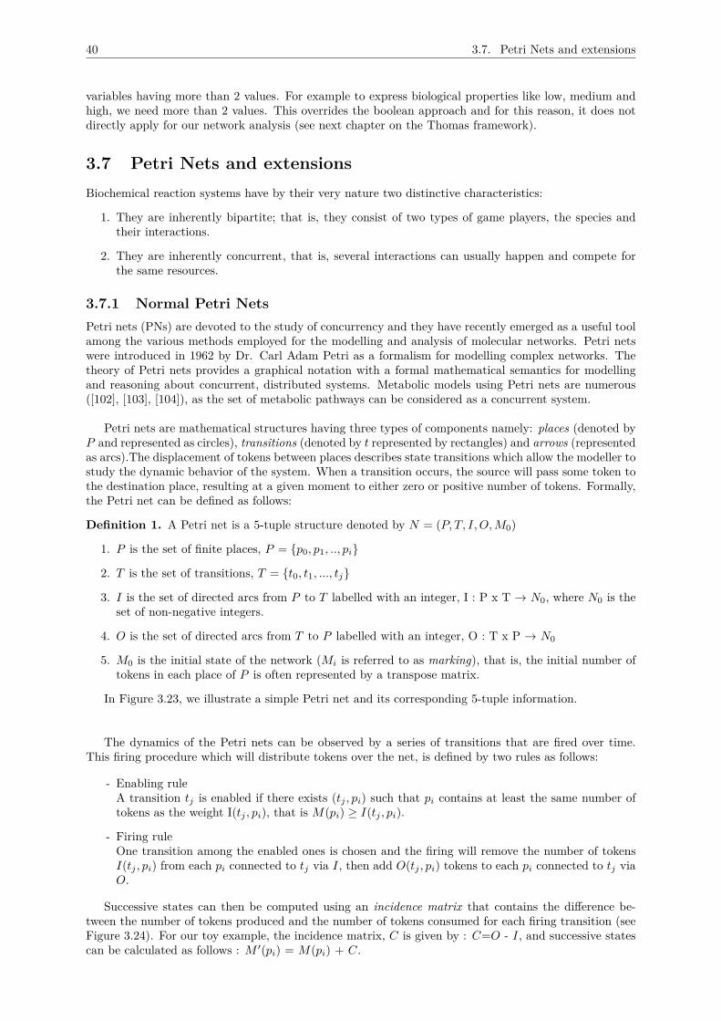
40 3.7. Petri Nets and extensions
variables having more than 2 values. For example to express biological properties like low, medium andhigh, we need more than 2 values. This overrides the boolean approach and for this reason, it does notdirectly apply for our network analysis (see next chapter on the Thomas framework).
3.7 Petri Nets and extensionsBiochemical reaction systems have by their very nature two distinctive characteristics:
1. They are inherently bipartite; that is, they consist of two types of game players, the species andtheir interactions.
2. They are inherently concurrent, that is, several interactions can usually happen and compete forthe same resources.
3.7.1 Normal Petri NetsPetri nets (PNs) are devoted to the study of concurrency and they have recently emerged as a useful toolamong the various methods employed for the modelling and analysis of molecular networks. Petri netswere introduced in 1962 by Dr. Carl Adam Petri as a formalism for modelling complex networks. Thetheory of Petri nets provides a graphical notation with a formal mathematical semantics for modellingand reasoning about concurrent, distributed systems. Metabolic models using Petri nets are numerous([102], [103], [104]), as the set of metabolic pathways can be considered as a concurrent system.
Petri nets are mathematical structures having three types of components namely: places (denoted byP and represented as circles), transitions (denoted by t represented by rectangles) and arrows (representedas arcs).The displacement of tokens between places describes state transitions which allow the modeller tostudy the dynamic behavior of the system. When a transition occurs, the source will pass some token tothe destination place, resulting at a given moment to either zero or positive number of tokens. Formally,the Petri net can be defined as follows:
Definition 1. A Petri net is a 5-tuple structure denoted by N = (P, T, I,O,M0)
1. P is the set of finite places, P = {p0, p1, .., pi}
2. T is the set of transitions, T = {t0, t1, ..., tj}
3. I is the set of directed arcs from P to T labelled with an integer, I : P x T → N0, where N0 is theset of non-negative integers.
4. O is the set of directed arcs from T to P labelled with an integer, O : T x P → N0
5. M0 is the initial state of the network (Mi is referred to as marking), that is, the initial number oftokens in each place of P is often represented by a transpose matrix.
In Figure 3.23, we illustrate a simple Petri net and its corresponding 5-tuple information.
The dynamics of the Petri nets can be observed by a series of transitions that are fired over time.This firing procedure which will distribute tokens over the net, is defined by two rules as follows:
- Enabling ruleA transition tj is enabled if there exists (tj , pi) such that pi contains at least the same number oftokens as the weight I(tj , pi), that is M(pi) ≥ I(tj , pi).
- Firing ruleOne transition among the enabled ones is chosen and the firing will remove the number of tokensI(tj , pi) from each pi connected to tj via I, then add O(tj , pi) tokens to each pi connected to tj viaO.
Successive states can then be computed using an incidence matrix that contains the difference be-tween the number of tokens produced and the number of tokens consumed for each firing transition (seeFigure 3.24). For our toy example, the incidence matrix, C is given by : C=O - I, and successive statescan be calculated as follows : M ′(pi) = M(pi) + C.
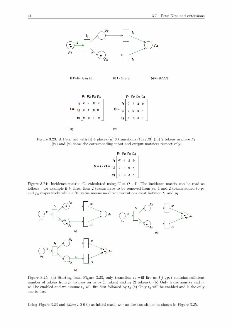
41 3.7. Petri Nets and extensions
Figure 3.23: A Petri net with (i) 4 places (ii) 3 transitions (t1,t2,t3) (iii) 2 tokens in place P1,(iv) and (v) show the corresponding input and output matrices respectively.
Figure 3.24: Incidence matrix, C, calculated using C = O - I. The incidence matrix can be read asfollows : for example if t1 fires, then 2 tokens have to be removed from p1, 1 and 2 tokens added to p2and p3 respectively while a "0" value means no direct transitions exist between t1 and p4.
Figure 3.25: (a) Starting from Figure 3.23, only transition t1 will fire as I(t1, p1) contains sufficientnumber of tokens from p1 to pass on to p2 (1 token) and p3 (2 tokens). (b) Only transitions t2 and t3will be enabled and we assume t2 will fire first followed by t3 (c) Only t3 will be enabled and is the onlyone to fire.
Using Figure 3.23 and M0=(2 0 0 0) as initial state, we can fire transitions as shown in Figure 3.25.
42 3.8. Rule-based frameworks
Advantages of Petri Nets:
1. We can do algebraic manipulations easily with the incidence matrix that allows us to view the"transfer" of tokens as well as the state transitions.
2. Petri nets are formalisms that are concurrent to FBA and EFM. In contrast to FBA and EFM,Petri nets are abstract to us since, instead of fluxes which are real values, tokens which are positiveintegers, are used.
3. The ability to use of CTL to view the evolution of Petri nets [105].
Disadvantages of Petri Nets:
1. Petri nets represent the fluxes in networks like FBA and EFM rather than regulations.
2. The inability to distinguish tokens in a Petri net.
For the entire metabolic network, the use of Petri nets would require too many information on thebiochemical reactions to choose the required tokens. To conclude, our focus is more on the regulationsrather than fluxes, therefore, we will not choose Petri nets as a formalism to address our question.
3.8 Rule-based frameworksBiochemical processes inside cells are regulated by intricate chemical reactions involving diverse moleculeswhich are catalysed by enzymes. The latter are in turn mediated by genes. In rule-based frameworks,these chemical reactions can be rewritten as rules with a well-defined syntax. Two commonly usedrule-based frameworks, namely BIOCHAM and Kappa, will be briefly discussed in this section.
3.8.1 BIOCHAMBIOCHAM (BIOCHemical Abstract Machine) is a rule-based language together with a software environ-ment for modelling biochemical signalling systems [106]. It also provides parameter identification andvalidation tools (uses temporal logic). BIOCHAM is designed using a logic programming setting and alanguage of reaction rules.
To specify a signalling system, BIOCHAM asks first to declare a "signature" which is an initial starting setof abstract molecules (multisets of them are called a solution) and it also asks for evolution rules(reactions)from which dynamical properties of the system can be formally established. BIOCHAM also offers thepossibility to choose within a set of semantics for models using one of the following frameworks :
1. asynchronous boolean networks (focuses on the presence/absence of molecules)
2. continuous-time Markov processes (focuses on numbers of molecules as a Markov chain)
3. ordinary differential equations (relies on molecular concentrations)
The syntax of BIOCHAM follows two forms namely : reaction networks (like biochemical reactions)and influence networks (like genetic and metabolic networks). In this text, we focus solely on the influencenetwork, as our metabolic network is regulated by many influencers (glucose, glutamine, etc).
SyntaxThe syntax for BIOCHAM is divided into four parts:
1. ObjectsAn object in BIOCHAM simply represents a biochemical species which can have one of the followingnotations :
• An object containing only letters and numbers represents a "simple" molecule.• An object with a "-" represents a complex and the "-" is commutative as well as associative.
This means that a-b is the same as b-a.• "Sites" can be integrated using the "v" operator. For example the two sites of phosphorylations1 and s2 for a given molecule m is given by m v (s1, s2).
Abstract objects, which are not molecules, can be prefixed with the @ character.
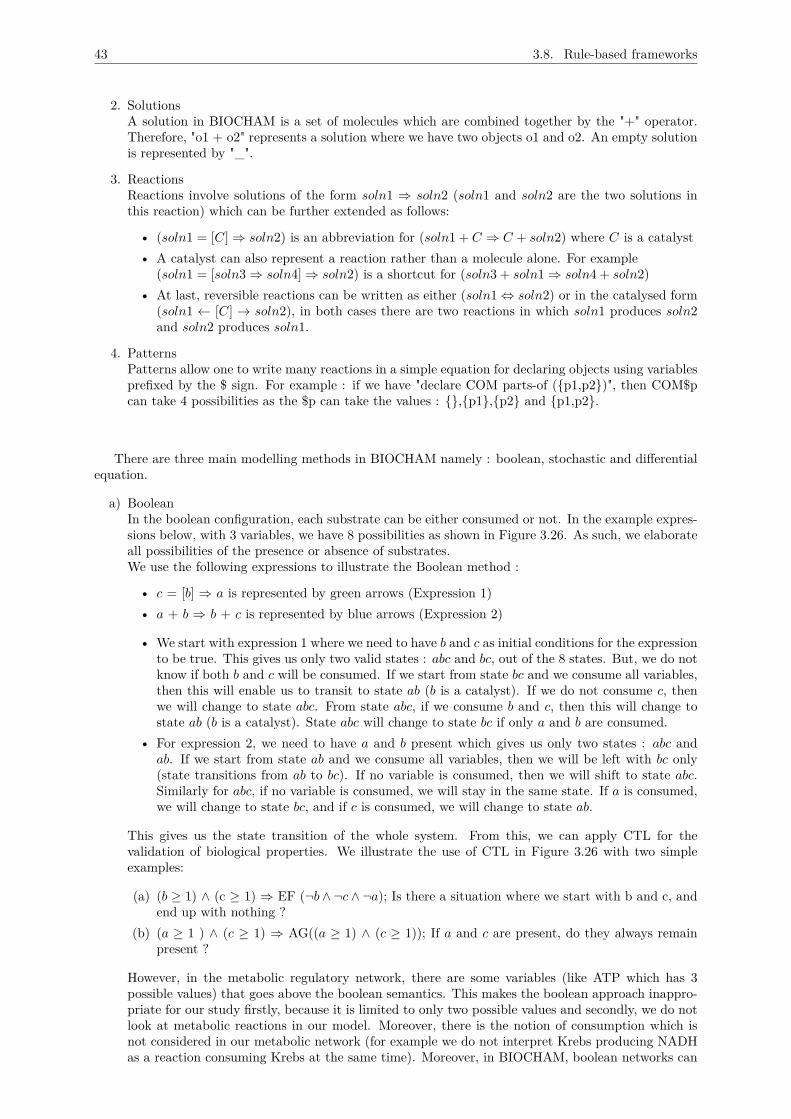
43 3.8. Rule-based frameworks
2. SolutionsA solution in BIOCHAM is a set of molecules which are combined together by the "+" operator.Therefore, "o1 + o2" represents a solution where we have two objects o1 and o2. An empty solutionis represented by "_".
3. ReactionsReactions involve solutions of the form soln1 ⇒ soln2 (soln1 and soln2 are the two solutions inthis reaction) which can be further extended as follows:
• (soln1 = [C]⇒ soln2) is an abbreviation for (soln1 + C ⇒ C + soln2) where C is a catalyst• A catalyst can also represent a reaction rather than a molecule alone. For example
(soln1 = [soln3⇒ soln4]⇒ soln2) is a shortcut for (soln3 + soln1⇒ soln4 + soln2)• At last, reversible reactions can be written as either (soln1⇔ soln2) or in the catalysed form
(soln1 ← [C] → soln2), in both cases there are two reactions in which soln1 produces soln2and soln2 produces soln1.
4. PatternsPatterns allow one to write many reactions in a simple equation for declaring objects using variablesprefixed by the $ sign. For example : if we have "declare COM parts-of ({p1,p2})", then COM$pcan take 4 possibilities as the $p can take the values : {},{p1},{p2} and {p1,p2}.
There are three main modelling methods in BIOCHAM namely : boolean, stochastic and differentialequation.
a) BooleanIn the boolean configuration, each substrate can be either consumed or not. In the example expres-sions below, with 3 variables, we have 8 possibilities as shown in Figure 3.26. As such, we elaborateall possibilities of the presence or absence of substrates.We use the following expressions to illustrate the Boolean method :
• c = [b] ⇒ a is represented by green arrows (Expression 1)• a + b ⇒ b + c is represented by blue arrows (Expression 2)
• We start with expression 1 where we need to have b and c as initial conditions for the expressionto be true. This gives us only two valid states : abc and bc, out of the 8 states. But, we do notknow if both b and c will be consumed. If we start from state bc and we consume all variables,then this will enable us to transit to state ab (b is a catalyst). If we do not consume c, thenwe will change to state abc. From state abc, if we consume b and c, then this will change tostate ab (b is a catalyst). State abc will change to state bc if only a and b are consumed.
• For expression 2, we need to have a and b present which gives us only two states : abc andab. If we start from state ab and we consume all variables, then we will be left with bc only(state transitions from ab to bc). If no variable is consumed, then we will shift to state abc.Similarly for abc, if no variable is consumed, we will stay in the same state. If a is consumed,we will change to state bc, and if c is consumed, we will change to state ab.
This gives us the state transition of the whole system. From this, we can apply CTL for thevalidation of biological properties. We illustrate the use of CTL in Figure 3.26 with two simpleexamples:
(a) (b ≥ 1) ∧ (c ≥ 1) ⇒ EF (¬b ∧ ¬c ∧ ¬a); Is there a situation where we start with b and c, andend up with nothing ?
(b) (a ≥ 1 ) ∧ (c ≥ 1) ⇒ AG((a ≥ 1) ∧ (c ≥ 1)); If a and c are present, do they always remainpresent ?
However, in the metabolic regulatory network, there are some variables (like ATP which has 3possible values) that goes above the boolean semantics. This makes the boolean approach inappro-priate for our study firstly, because it is limited to only two possible values and secondly, we do notlook at metabolic reactions in our model. Moreover, there is the notion of consumption which isnot considered in our metabolic network (for example we do not interpret Krebs producing NADHas a reaction consuming Krebs at the same time). Moreover, in BIOCHAM, boolean networks can
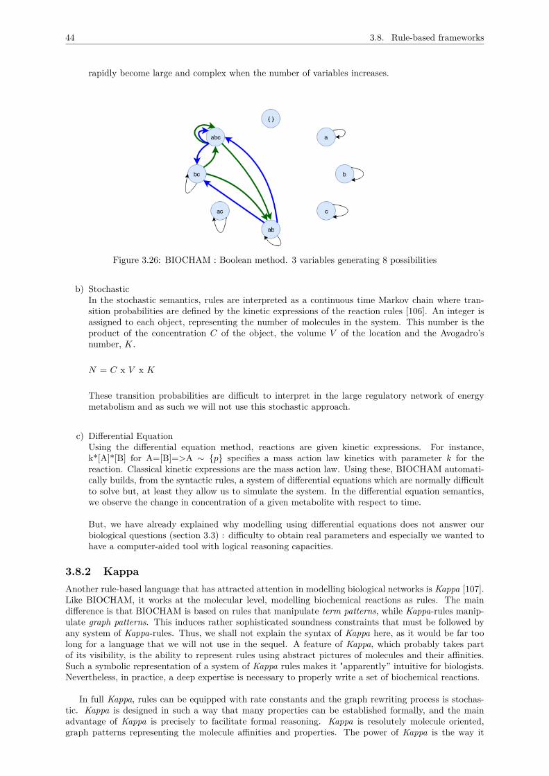
44 3.8. Rule-based frameworks
rapidly become large and complex when the number of variables increases.
Figure 3.26: BIOCHAM : Boolean method. 3 variables generating 8 possibilities
b) StochasticIn the stochastic semantics, rules are interpreted as a continuous time Markov chain where tran-sition probabilities are defined by the kinetic expressions of the reaction rules [106]. An integer isassigned to each object, representing the number of molecules in the system. This number is theproduct of the concentration C of the object, the volume V of the location and the Avogadro’snumber, K.
N = C x V x K
These transition probabilities are difficult to interpret in the large regulatory network of energymetabolism and as such we will not use this stochastic approach.
c) Differential EquationUsing the differential equation method, reactions are given kinetic expressions. For instance,k*[A]*[B] for A=[B]=>A ∼ {p} specifies a mass action law kinetics with parameter k for thereaction. Classical kinetic expressions are the mass action law. Using these, BIOCHAM automati-cally builds, from the syntactic rules, a system of differential equations which are normally difficultto solve but, at least they allow us to simulate the system. In the differential equation semantics,we observe the change in concentration of a given metabolite with respect to time.
But, we have already explained why modelling using differential equations does not answer ourbiological questions (section 3.3) : difficulty to obtain real parameters and especially we wanted tohave a computer-aided tool with logical reasoning capacities.
3.8.2 KappaAnother rule-based language that has attracted attention in modelling biological networks is Kappa [107].Like BIOCHAM, it works at the molecular level, modelling biochemical reactions as rules. The maindifference is that BIOCHAM is based on rules that manipulate term patterns, while Kappa-rules manip-ulate graph patterns. This induces rather sophisticated soundness constraints that must be followed byany system of Kappa-rules. Thus, we shall not explain the syntax of Kappa here, as it would be far toolong for a language that we will not use in the sequel. A feature of Kappa, which probably takes partof its visibility, is the ability to represent rules using abstract pictures of molecules and their affinities.Such a symbolic representation of a system of Kappa rules makes it "apparently” intuitive for biologists.Nevertheless, in practice, a deep expertise is necessary to properly write a set of biochemical reactions.
In full Kappa, rules can be equipped with rate constants and the graph rewriting process is stochas-tic. Kappa is designed in such a way that many properties can be established formally, and the mainadvantage of Kappa is precisely to facilitate formal reasoning. Kappa is resolutely molecule oriented,graph patterns representing the molecule affinities and properties. The power of Kappa is the way it
45 3.9. Conclusion of the chapter
deals with the combinatorial complexity, which is among the main challenges in modelling complex net-works. If one does not want to abstract molecular processes in the cell, then there is the possibility toabstract behaviours and make them "emerge” from a huge number of such elementary molecular processes.
So, Kappa is probably the most deeply formal framework dedicated to modelling molecular processesin the cell. But paradoxically, it is far too concrete with respect to our motivation to understand the maincausality mechanisms in cell metabolism regulation because, it is dedicated to rules at the molecular level.
According to this important consideration, BIOCHAM would be less “tied” to concrete molecularreactions, as the terms used in BIOCHAM can represent arbitrarily abstract concepts. It remains thatBIOCHAM is oriented to the modelling of signaling reactions rather that regulation mechanisms.
3.9 Conclusion of the chapterAn array of rigorous techniques for modelling biological networks has been outlined in this chapter witha particular attention to the strengths and weaknesses of each framework. The choice between qualita-tive and quantitative formalisms resides in the biological question under consideration. These modellingframeworks are representation of the main possible approaches and they are complementary to each other.The main weakness of the frameworks described here is that metabolic regulations are neglected and seenas side phenomena.
Interestingly, some of the criteria we would be looking forward to for our choice of formalism includea high degree of abstraction for regulation of metabolism with a selection of important variables support-ing this regulation. Our main motive is to understand the underlying causalities in metabolic regulationsand we want to be able to use a computer-aided approach to study these causalities. So, formal methodsare clearly suitable because logic and formal methods can establish proofs using software tools. Thechoice of our framework will be explained in the next chapter.
CHAPTER 4THE THOMAS MODELLING
FRAMEWORK
4.1 IntroductionIn the late 1990’s, formalisms based on differential equation were de-facto the main methods used inthe modelling of complex biological systems [109] : often, biological experiments based on concentrationlevel measurements reflect changes of certain molecular species along time (like gene activity via one ofits products). Such quantitative dynamics, where several variables interact to produce curves of realnumbers in function of time are often captured in systems of ordinary differential equation (ODE) ina rather natural way. The representation of temporal aspects of systems (rate of change of physicalquantities) in biology, and as a matter of fact in many other complex systems, is one of the most frequentapplication of ODEs. The real strong difficulties begin when we try to identify the ODE parameters.Moreover, biological systems are often non-deterministic ones, but ODE only encode deterministic tra-jectories, due to a hypothesis of "large number of molecules" that justifies the continuous setting of ODE.In molecular biology, we cannot ignore a common feature that biological complex systems exhibit : theirnon-deterministic behaviours.
This chapter enlists some motivations of Réné Thomas in the search of a more simplistic discrete approachto the modelling of gene networks for the study of their dynamics. After a rigorous definition of the for-malism, we will see how other researchers have integrated useful features from computer science addingmore power to his formalism. Later on in chapters 7 and 8, we will show how the Thomas’ modellingframework scales well for our metabolic network with 13 variables and 100 parameters, representing, upto our knowledge, the largest network modelled using this framework.
4.1.1 MotivationFinding kinetic parameters is a major bottleneck in the study of dynamics of complex systems. ODEsare often too precise, with parameters belonging real numbers, to be used in cellular biology, due toinsufficient precise measurement capabilities. Moreover, there are many large intervals of values whereany change of parameters in the differential equation does not modify the observable end result.
To gain insight into the interaction and regulation of biological systems, Réné Thomas proposed a booleanframework that is close enough to actual biological regulatory networks, which manifest themselves in aqualitative manner. In this context, an object is either activated or inhibited. In genetics, this correspondsto an ON/OFF state of genes which can occur during gene expressions or at the level of transcription.The motive of the next subsection is to detail how Réné Thomas achieved his boolean approach in amanner that can be formally seen as a slight extension of boolean networks described in the previouschapter. Then, the approach was later mathematically defined and extended by Houssine Snoussi [110].Here, we directly define the Snoussi version with formal extension.
4.1.2 A variant of automata networksLiving cells are in a state of ceaseless activity. The way organisms are constructed, how they function,how they react to external environment and more generally their behaviour, are partly monitored bygenes. These controls follow a series of activations and inhibitions, which were previously modelled inODE as sigmoids. This is nicely captured in Figure 4.1, where an activation is translated into an in-creasing sigmoid (green curve) and an inhibition into a decreasing sigmoid (red curve). Since we are
46
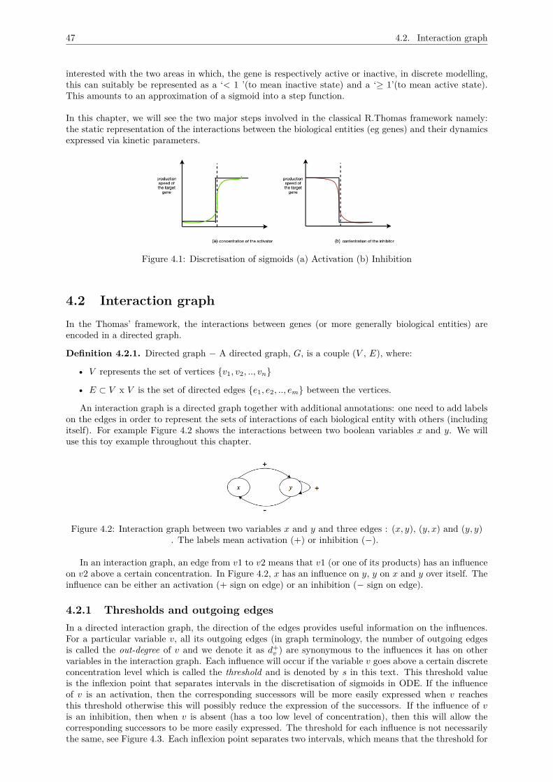
47 4.2. Interaction graph
interested with the two areas in which, the gene is respectively active or inactive, in discrete modelling,this can suitably be represented as a ‘< 1 ’(to mean inactive state) and a ‘≥ 1’(to mean active state).This amounts to an approximation of a sigmoid into a step function.
In this chapter, we will see the two major steps involved in the classical R.Thomas framework namely:the static representation of the interactions between the biological entities (eg genes) and their dynamicsexpressed via kinetic parameters.
Figure 4.1: Discretisation of sigmoids (a) Activation (b) Inhibition
4.2 Interaction graphIn the Thomas’ framework, the interactions between genes (or more generally biological entities) areencoded in a directed graph.
Definition 4.2.1. Directed graph − A directed graph, G, is a couple (V , E), where:
• V represents the set of vertices {v1, v2, .., vn}
• E ⊂ V x V is the set of directed edges {e1, e2, .., em} between the vertices.
An interaction graph is a directed graph together with additional annotations: one need to add labelson the edges in order to represent the sets of interactions of each biological entity with others (includingitself). For example Figure 4.2 shows the interactions between two boolean variables x and y. We willuse this toy example throughout this chapter.
Figure 4.2: Interaction graph between two variables x and y and three edges : (x, y), (y, x) and (y, y). The labels mean activation (+) or inhibition (−).
In an interaction graph, an edge from v1 to v2 means that v1 (or one of its products) has an influenceon v2 above a certain concentration. In Figure 4.2, x has an influence on y, y on x and y over itself. Theinfluence can be either an activation (+ sign on edge) or an inhibition (− sign on edge).
4.2.1 Thresholds and outgoing edgesIn a directed interaction graph, the direction of the edges provides useful information on the influences.For a particular variable v, all its outgoing edges (in graph terminology, the number of outgoing edgesis called the out-degree of v and we denote it as d+
v ) are synonymous to the influences it has on othervariables in the interaction graph. Each influence will occur if the variable v goes above a certain discreteconcentration level which is called the threshold and is denoted by s in this text. This threshold valueis the inflexion point that separates intervals in the discretisation of sigmoids in ODE. If the influenceof v is an activation, then the corresponding successors will be more easily expressed when v reachesthis threshold otherwise this will possibly reduce the expression of the successors. If the influence of vis an inhibition, then when v is absent (has a too low level of concentration), then this will allow thecorresponding successors to be more easily expressed. The threshold for each influence is not necessarilythe same, see Figure 4.3. Each inflexion point separates two intervals, which means that the threshold for
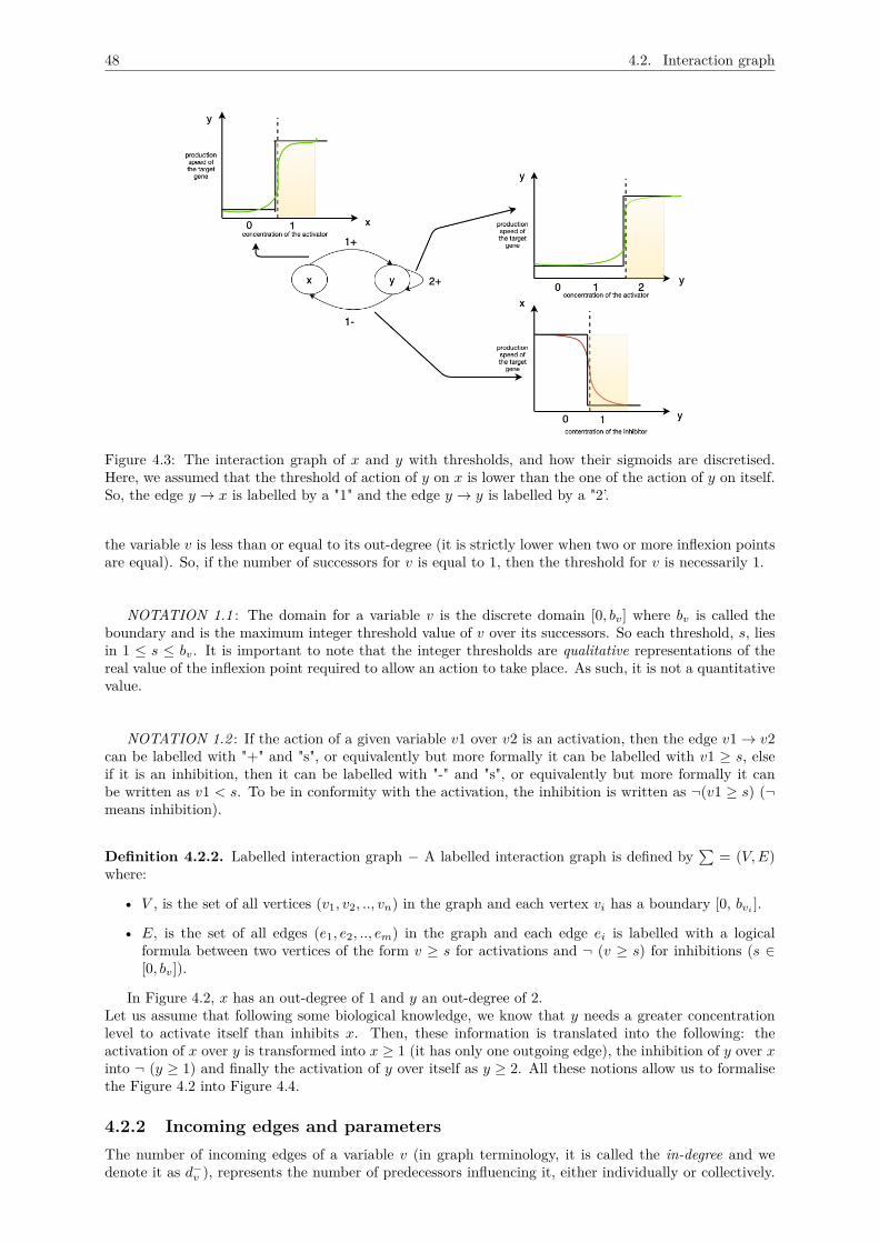
48 4.2. Interaction graph
Figure 4.3: The interaction graph of x and y with thresholds, and how their sigmoids are discretised.Here, we assumed that the threshold of action of y on x is lower than the one of the action of y on itself.So, the edge y → x is labelled by a "1" and the edge y → y is labelled by a "2’.
the variable v is less than or equal to its out-degree (it is strictly lower when two or more inflexion pointsare equal). So, if the number of successors for v is equal to 1, then the threshold for v is necessarily 1.
NOTATION 1.1 : The domain for a variable v is the discrete domain [0, bv] where bv is called theboundary and is the maximum integer threshold value of v over its successors. So each threshold, s, liesin 1 ≤ s ≤ bv. It is important to note that the integer thresholds are qualitative representations of thereal value of the inflexion point required to allow an action to take place. As such, it is not a quantitativevalue.
NOTATION 1.2 : If the action of a given variable v1 over v2 is an activation, then the edge v1→ v2can be labelled with "+" and "s", or equivalently but more formally it can be labelled with v1 ≥ s, elseif it is an inhibition, then it can be labelled with "-" and "s", or equivalently but more formally it canbe written as v1 < s. To be in conformity with the activation, the inhibition is written as ¬(v1 ≥ s) (¬means inhibition).
Definition 4.2.2. Labelled interaction graph − A labelled interaction graph is defined by∑
= (V,E)where:
• V , is the set of all vertices (v1, v2, .., vn) in the graph and each vertex vi has a boundary [0, bvi ].
• E, is the set of all edges (e1, e2, .., em) in the graph and each edge ei is labelled with a logicalformula between two vertices of the form v ≥ s for activations and ¬ (v ≥ s) for inhibitions (s ∈[0, bv]).
In Figure 4.2, x has an out-degree of 1 and y an out-degree of 2.Let us assume that following some biological knowledge, we know that y needs a greater concentrationlevel to activate itself than inhibits x. Then, these information is translated into the following: theactivation of x over y is transformed into x ≥ 1 (it has only one outgoing edge), the inhibition of y over xinto ¬ (y ≥ 1) and finally the activation of y over itself as y ≥ 2. All these notions allow us to formalisethe Figure 4.2 into Figure 4.4.
4.2.2 Incoming edges and parametersThe number of incoming edges of a variable v (in graph terminology, it is called the in-degree and wedenote it as d−v ), represents the number of predecessors influencing it, either individually or collectively.
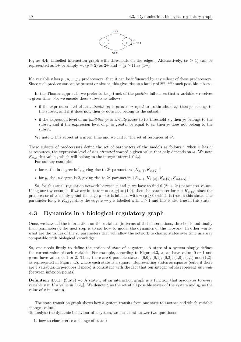
49 4.3. Dynamics in a biological regulatory graph
Figure 4.4: Labelled interaction graph with thresholds on the edges. Alternatively, (x ≥ 1) can berepresented as 1+ or simply +, (y ≥ 2) as 2+ and ¬ (y ≥ 1) as (1−)
If a variable v has p1, p2, .., pn predecessors, then it can be influenced by any subset of these predecessors.Since each predecessor can be present or absent, this gives rise to a family of 2in_degv such possible subsets.
In the Thomas approach, we prefer to keep track of the positive influences that a variable v receivesa given time. So, we encode these subsets as follows:
• if the expression level of an activator pi is greater or equal to its threshold si, then pi belongs tothe subset, and if it does not, then pi does not belong to the subset.
• if the expression level of an inhibitor pi is strictly lower to its threshold si, then pi belongs to thesubset, and if the expression level of pi is greater or equal to si, then pi does not belong to thesubset.
We note ω this subset at a given time and we call it "the set of resources of v".
These subsets of predecessors define the set of parameters of the models as follows : when v has ωas resources, the expression level of v is attracted toward a given value that only depends on ω. We noteKv,ω this value , which will belong to the integer interval [0,bv].
For our toy example:
• for x, the in-degree is 1, giving rise to 21 parameters {Kx,{},Kx,{y}}
• for y, the in-degree is 2, giving rise to 22 parameters {Ky,{},Ky,{x},Ky,{y},Ky,{x,y}}
So, for this small regulation network between x and y, we have to find 6 (21 + 22) parameter values.Using our toy example, if we are in state η = (x, y) = (1,0), then the parameter for x is Kx,{y} since thepredecessor of x is only y and the edge y → x is labelled with ¬ (y ≥ 0) which is true in this state. Theparameter for y is Ky,{x} since the edge x→ y is labelled with x ≥ 1 and this is also true in this state.
4.3 Dynamics in a biological regulatory graphOnce, we have all the information on the variables (in terms of their interactions, thresholds and finallytheir parameters), the next step is to see how to model the dynamics of the network. In other words,what are the values of the K parameters that will allow the network to change states over time in a waycompatible with biological knowledge.
So, one needs firstly to define the notion of state of a system. A state of a system simply definesthe current value of each variable. For example, according to Figure 4.3, x can have values 0 or 1 andy can have values 0, 1 or 2. Thus, there are 6 possible states: (0,0), (0,1), (0,2), (1,0), (1,1) and (1,2),as represented in Figure 4.5, where each state is a square. Representing states as squares (cube if thereare 3 variables, hypercubes if more) is consistent with the fact that our integer values represent intervals(between inflexion points).
Definition 4.3.1. (State) −: A state η of an interaction graph is a function that associates to everyvariable v in V a value in [0, bv]. We denote ζ as the set of all possible states of the system and ηv as thevalue of v in state η.
The state transition graph shows how a system transits from one state to another and which variablechanges values.To analyse the dynamic behaviour of a system, we must first answer two questions:
1. how to characterise a change of state ?
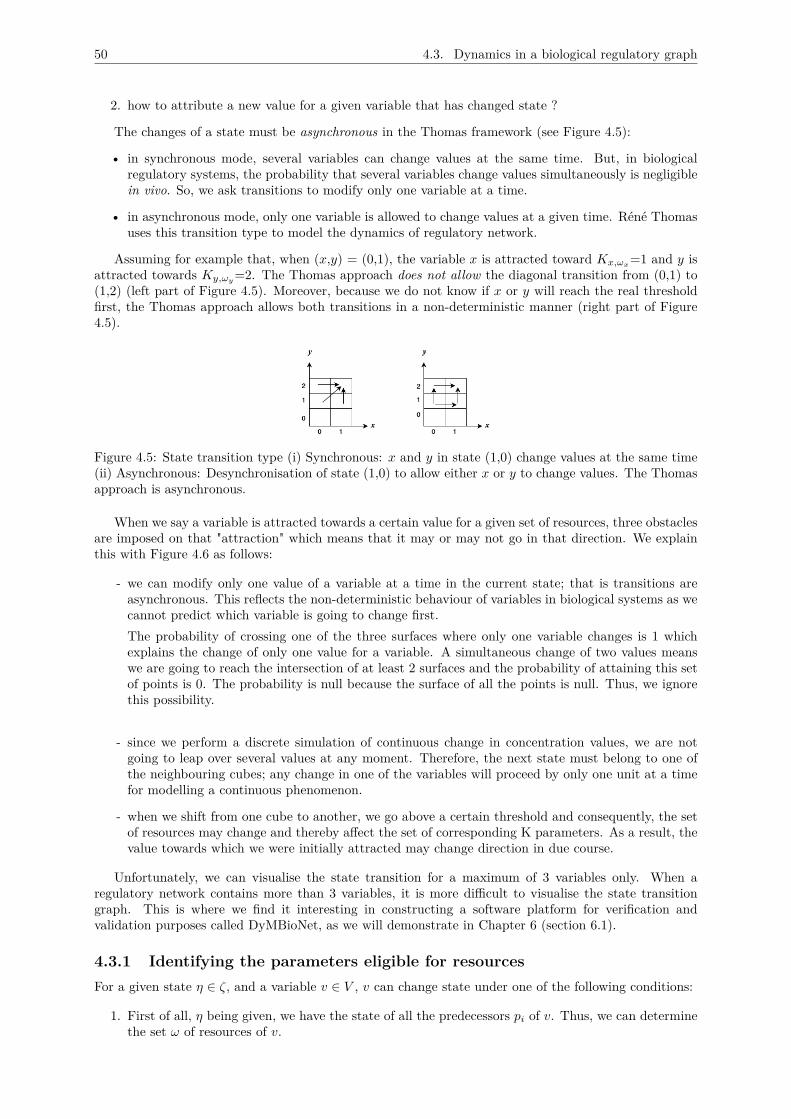
50 4.3. Dynamics in a biological regulatory graph
2. how to attribute a new value for a given variable that has changed state ?
The changes of a state must be asynchronous in the Thomas framework (see Figure 4.5):
• in synchronous mode, several variables can change values at the same time. But, in biologicalregulatory systems, the probability that several variables change values simultaneously is negligiblein vivo. So, we ask transitions to modify only one variable at a time.
• in asynchronous mode, only one variable is allowed to change values at a given time. Réné Thomasuses this transition type to model the dynamics of regulatory network.
Assuming for example that, when (x,y) = (0,1), the variable x is attracted toward Kx,ωx=1 and y is
attracted towards Ky,ωy=2. The Thomas approach does not allow the diagonal transition from (0,1) to
(1,2) (left part of Figure 4.5). Moreover, because we do not know if x or y will reach the real thresholdfirst, the Thomas approach allows both transitions in a non-deterministic manner (right part of Figure4.5).
Figure 4.5: State transition type (i) Synchronous: x and y in state (1,0) change values at the same time(ii) Asynchronous: Desynchronisation of state (1,0) to allow either x or y to change values. The Thomasapproach is asynchronous.
When we say a variable is attracted towards a certain value for a given set of resources, three obstaclesare imposed on that "attraction" which means that it may or may not go in that direction. We explainthis with Figure 4.6 as follows:
- we can modify only one value of a variable at a time in the current state; that is transitions areasynchronous. This reflects the non-deterministic behaviour of variables in biological systems as wecannot predict which variable is going to change first.The probability of crossing one of the three surfaces where only one variable changes is 1 whichexplains the change of only one value for a variable. A simultaneous change of two values meanswe are going to reach the intersection of at least 2 surfaces and the probability of attaining this setof points is 0. The probability is null because the surface of all the points is null. Thus, we ignorethis possibility.
- since we perform a discrete simulation of continuous change in concentration values, we are notgoing to leap over several values at any moment. Therefore, the next state must belong to one ofthe neighbouring cubes; any change in one of the variables will proceed by only one unit at a timefor modelling a continuous phenomenon.
- when we shift from one cube to another, we go above a certain threshold and consequently, the setof resources may change and thereby affect the set of corresponding K parameters. As a result, thevalue towards which we were initially attracted may change direction in due course.
Unfortunately, we can visualise the state transition for a maximum of 3 variables only. When aregulatory network contains more than 3 variables, it is more difficult to visualise the state transitiongraph. This is where we find it interesting in constructing a software platform for verification andvalidation purposes called DyMBioNet, as we will demonstrate in Chapter 6 (section 6.1).
4.3.1 Identifying the parameters eligible for resourcesFor a given state η ∈ ζ, and a variable v ∈ V , v can change state under one of the following conditions:
1. First of all, η being given, we have the state of all the predecessors pi of v. Thus, we can determinethe set ω of resources of v.
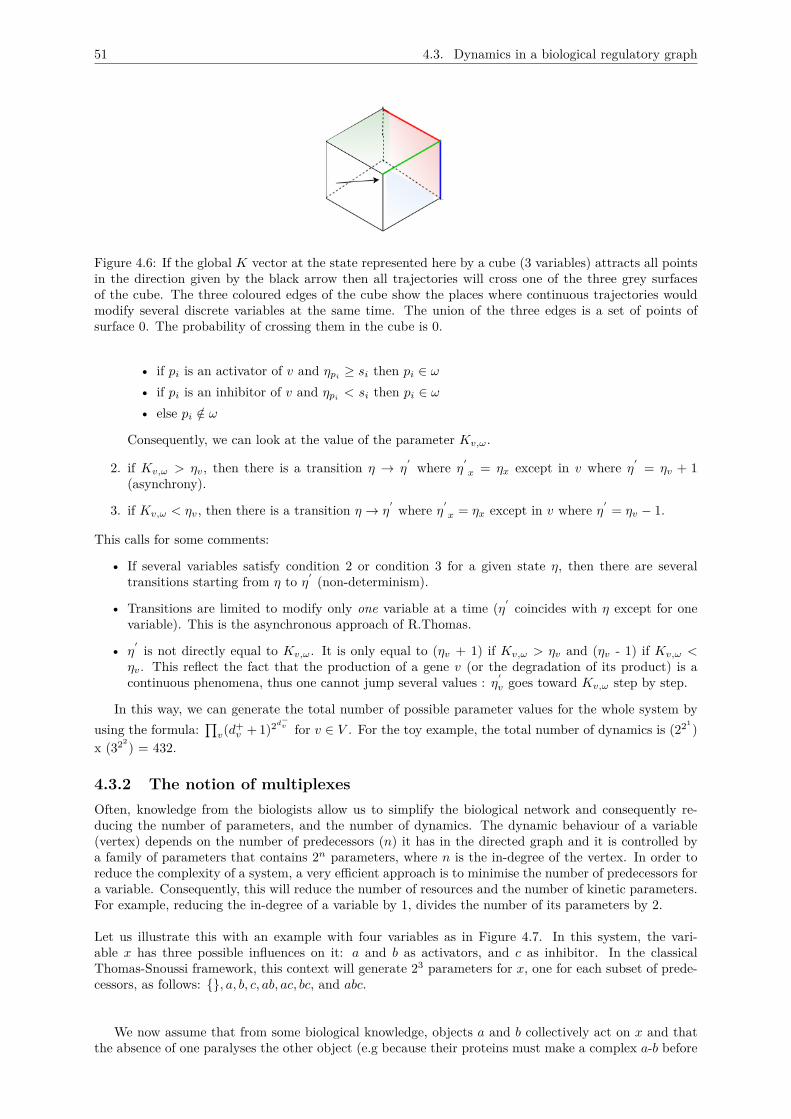
51 4.3. Dynamics in a biological regulatory graph
Figure 4.6: If the global K vector at the state represented here by a cube (3 variables) attracts all pointsin the direction given by the black arrow then all trajectories will cross one of the three grey surfacesof the cube. The three coloured edges of the cube show the places where continuous trajectories wouldmodify several discrete variables at the same time. The union of the three edges is a set of points ofsurface 0. The probability of crossing them in the cube is 0.
• if pi is an activator of v and ηpi≥ si then pi ∈ ω
• if pi is an inhibitor of v and ηpi< si then pi ∈ ω
• else pi /∈ ω
Consequently, we can look at the value of the parameter Kv,ω.
2. if Kv,ω > ηv, then there is a transition η → η′ where η′x = ηx except in v where η′ = ηv + 1
(asynchrony).
3. if Kv,ω < ηv, then there is a transition η → η′ where η′x = ηx except in v where η′ = ηv − 1.
This calls for some comments:
• If several variables satisfy condition 2 or condition 3 for a given state η, then there are severaltransitions starting from η to η′ (non-determinism).
• Transitions are limited to modify only one variable at a time (η′ coincides with η except for onevariable). This is the asynchronous approach of R.Thomas.
• η′ is not directly equal to Kv,ω. It is only equal to (ηv + 1) if Kv,ω > ηv and (ηv - 1) if Kv,ω <ηv. This reflect the fact that the production of a gene v (or the degradation of its product) is acontinuous phenomena, thus one cannot jump several values : η′v goes toward Kv,ω step by step.
In this way, we can generate the total number of possible parameter values for the whole system byusing the formula:
∏v(d+
v + 1)2d−v for v ∈ V . For the toy example, the total number of dynamics is (221)
x (322) = 432.
4.3.2 The notion of multiplexesOften, knowledge from the biologists allow us to simplify the biological network and consequently re-ducing the number of parameters, and the number of dynamics. The dynamic behaviour of a variable(vertex) depends on the number of predecessors (n) it has in the directed graph and it is controlled bya family of parameters that contains 2n parameters, where n is the in-degree of the vertex. In order toreduce the complexity of a system, a very efficient approach is to minimise the number of predecessors fora variable. Consequently, this will reduce the number of resources and the number of kinetic parameters.For example, reducing the in-degree of a variable by 1, divides the number of its parameters by 2.
Let us illustrate this with an example with four variables as in Figure 4.7. In this system, the vari-able x has three possible influences on it: a and b as activators, and c as inhibitor. In the classicalThomas-Snoussi framework, this context will generate 23 parameters for x, one for each subset of prede-cessors, as follows: {}, a, b, c, ab, ac, bc, and abc.
We now assume that from some biological knowledge, objects a and b collectively act on x and thatthe absence of one paralyses the other object (e.g because their proteins must make a complex a-b before
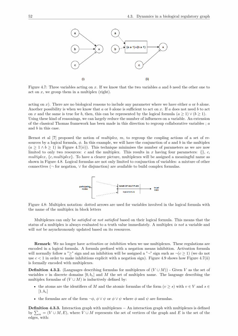
52 4.3. Dynamics in a biological regulatory graph
Figure 4.7: Three variables acting on x. If we know that the two variables a and b need the other one toact on x, we group them in a multiplex (right).
acting on x). There are no biological reasons to include any parameter where we have either a or b alone.Another possibility is when we know that a or b alone is sufficient to act on x. If a does not need b to acton x and the same is true for b, then, this can be represented by the logical formula (a ≥ 1) ∨ (b ≥ 1).Using these kind of reasonings, we can largely reduce the number of influences on a variable. An extensionof the classical Thomas framework has been made in this direction to regroup collaborative variables ; aand b in this case.
Bernot et al [?] proposed the notion of multiplex, m, to regroup the coupling actions of a set of re-sources by a logical formula, φ. In this example, we will have the conjunction of a and b in the multiplex(a ≥ 1 ∧ b ≥ 1) in Figure 4.7(ii)). This technique minimises the number of parameters as we are nowlimited to only two resources: c and the multiplex. This results in x having four parameters: {}, c,multiplex, {c,multiplex}. To have a clearer picture, multiplexes will be assigned a meaningful name asshown in Figure 4.8. Logical formulas are not only limited to conjunction of variables: a mixture of otherconnectives (¬ for negation, ∨ for disjunction) are available to build complex formulas.
Figure 4.8: Multiplex notation: dotted arrows are used for variables involved in the logical formula withthe name of the multiplex in block letters
Multiplexes can only be satisfied or not satisfied based on their logical formula. This means that thestatus of a multiplex is always evaluated to a truth value immediately. A multiplex is not a variable andwill not be asynchronously updated based on its resources.
Remark: We no longer have activation or inhibition when we use multiplexes. These regulations areencoded in a logical formula. A formula prefixed with a negation means inhibition. Activation formulawill normally follow a "≥" sign and an inhibition will be assigned a "¬" sign such as ¬(c ≥ 1) (we do notuse c < 1 in order to make inhibitions explicit with a negation sign). Figure 4.9 shows how Figure 4.7(ii)is formally encoded with multiplexes.
Definition 4.3.2. (Languages describing formulas for multiplexes of (V ∪M)) - Given V as the set ofvariables v in discrete domains [0, bv] and M the set of multiplex name. The language describing themultiplex formulas of (V ∪M) is inductively defined by:
• the atoms are the identifiers of M and the atomic formulas of the form (v ≥ s) with v ∈ V and s ∈[1, bv]
• the formulas are of the form ¬φ, φ ∨ ψ or φ ∨ ψ where φ and ψ are formulas.
Definition 4.3.3. Interaction graph with multiplexes − An interaction graph with multiplexes is definedby∑
m = (V ∪M,E), where V ∪M represents the set of vertices of the graph and E is the set of theedges, with:
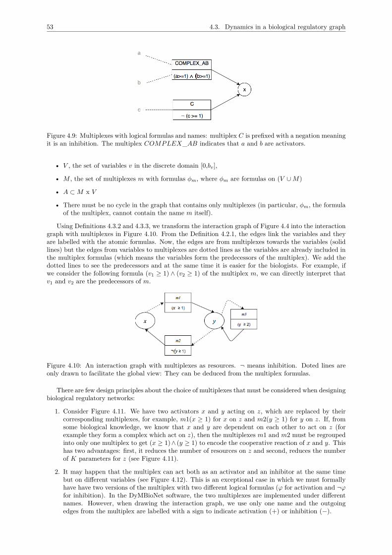
53 4.3. Dynamics in a biological regulatory graph
Figure 4.9: Multiplexes with logical formulas and names: multiplex C is prefixed with a negation meaningit is an inhibition. The multiplex COMPLEX_AB indicates that a and b are activators.
• V , the set of variables v in the discrete domain [0,bv],
• M , the set of multiplexes m with formulas φm, where φm are formulas on (V ∪M)
• A ⊂M x V
• There must be no cycle in the graph that contains only multiplexes (in particular, φm, the formulaof the multiplex, cannot contain the name m itself).
Using Definitions 4.3.2 and 4.3.3, we transform the interaction graph of Figure 4.4 into the interactiongraph with multiplexes in Figure 4.10. From the Definition 4.2.1, the edges link the variables and theyare labelled with the atomic formulas. Now, the edges are from multiplexes towards the variables (solidlines) but the edges from variables to multiplexes are dotted lines as the variables are already included inthe multiplex formulas (which means the variables form the predecessors of the multiplex). We add thedotted lines to see the predecessors and at the same time it is easier for the biologists. For example, ifwe consider the following formula (v1 ≥ 1) ∧ (v2 ≥ 1) of the multiplex m, we can directly interpret thatv1 and v2 are the predecessors of m.
Figure 4.10: An interaction graph with multiplexes as resources. ¬ means inhibition. Doted lines areonly drawn to facilitate the global view: They can be deduced from the multiplex formulas.
There are few design principles about the choice of multiplexes that must be considered when designingbiological regulatory networks:
1. Consider Figure 4.11. We have two activators x and y acting on z, which are replaced by theircorresponding multiplexes, for example, m1(x ≥ 1) for x on z and m2(y ≥ 1) for y on z. If, fromsome biological knowledge, we know that x and y are dependent on each other to act on z (forexample they form a complex which act on z), then the multiplexes m1 and m2 must be regroupedinto only one multiplex to get (x ≥ 1)∧ (y ≥ 1) to encode the cooperative reaction of x and y. Thishas two advantages: first, it reduces the number of resources on z and second, reduces the numberof K parameters for z (see Figure 4.11).
2. It may happen that the multiplex can act both as an activator and an inhibitor at the same timebut on different variables (see Figure 4.12). This is an exceptional case in which we must formallyhave have two versions of the multiplex with two different logical formulas (ϕ for activation and ¬ϕfor inhibition). In the DyMBioNet software, the two multiplexes are implemented under differentnames. However, when drawing the interaction graph, we use only one name and the outgoingedges from the multiplex are labelled with a sign to indicate activation (+) or inhibition (−).
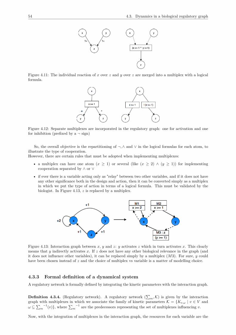
54 4.3. Dynamics in a biological regulatory graph
Figure 4.11: The individual reaction of x over z and y over z are merged into a multiplex with a logicalformula.
Figure 4.12: Separate multiplexes are incorporated in the regulatory graph: one for activation and onefor inhibition (prefixed by a ¬ sign)
So, the overall objective is the repartitioning of ¬,∧ and ∨ in the logical formulas for each atom, toillustrate the type of cooperation.However, there are certain rules that must be adopted when implementing multiplexes:
• a multiplex can have one atom (x ≥ 1) or several (like (x ≥ 2) ∧ (y ≥ 1)) for implementingcooperation separated by ∧ or ∨
• if ever there is a variable acting only as "relay" between two other variables, and if it does not haveany other significance both in the design and action, then it can be converted simply as a multiplexin which we put the type of action in terms of a logical formula. This must be validated by thebiologist. In Figure 4.13, z is replaced by a multiplex.
Figure 4.13: Interaction graph between x, y and z: y activates z which in turn activates x. This clearlymeans that y indirectly activates x. If z does not have any other biological relevance in the graph (andit does not influence other variables), it can be replaced simply by a multiplex (M3). For sure, y couldhave been chosen instead of z and the choice of multiplex vs variable is a matter of modelling choice.
4.3.3 Formal definition of a dynamical systemA regulatory network is formally defined by integrating the kinetic parameters with the interaction graph.
Definition 4.3.4. (Regulatory network). A regulatory network (∑
m,K) is given by the interactiongraph with multiplexes in which we associate the family of kinetic parameters K = {Kv,ω | v ∈ V andω ⊆
∑m−1(v)}, where
∑m−1 are the predecessors representing the set of multiplexes influencing v.
Now, with the integration of multiplexes in the interaction graph, the resources for each variable are the
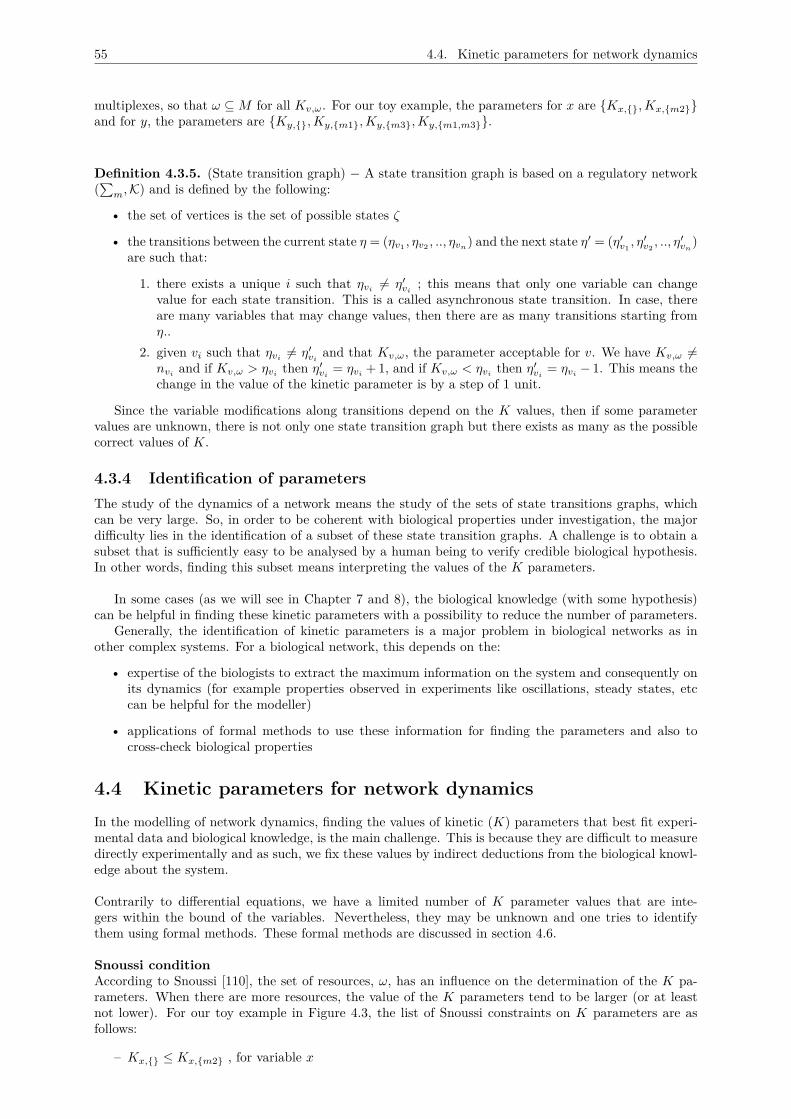
55 4.4. Kinetic parameters for network dynamics
multiplexes, so that ω ⊆M for all Kv,ω. For our toy example, the parameters for x are {Kx,{},Kx,{m2}}and for y, the parameters are {Ky,{},Ky,{m1},Ky,{m3},Ky,{m1,m3}}.
Definition 4.3.5. (State transition graph) − A state transition graph is based on a regulatory network(∑
m,K) and is defined by the following:
• the set of vertices is the set of possible states ζ
• the transitions between the current state η = (ηv1 , ηv2 , .., ηvn) and the next state η′ = (η′v1, η′v2
, .., η′vn)
are such that:
1. there exists a unique i such that ηvi6= η′vi
; this means that only one variable can changevalue for each state transition. This is a called asynchronous state transition. In case, thereare many variables that may change values, then there are as many transitions starting fromη..
2. given vi such that ηvi6= η′vi
and that Kv,ω, the parameter acceptable for v. We have Kv,ω 6=nvi
and if Kv,ω > ηvithen η′vi
= ηvi+ 1, and if Kv,ω < ηvi
then η′vi= ηvi
− 1. This means thechange in the value of the kinetic parameter is by a step of 1 unit.
Since the variable modifications along transitions depend on the K values, then if some parametervalues are unknown, there is not only one state transition graph but there exists as many as the possiblecorrect values of K.
4.3.4 Identification of parametersThe study of the dynamics of a network means the study of the sets of state transitions graphs, whichcan be very large. So, in order to be coherent with biological properties under investigation, the majordifficulty lies in the identification of a subset of these state transition graphs. A challenge is to obtain asubset that is sufficiently easy to be analysed by a human being to verify credible biological hypothesis.In other words, finding this subset means interpreting the values of the K parameters.
In some cases (as we will see in Chapter 7 and 8), the biological knowledge (with some hypothesis)can be helpful in finding these kinetic parameters with a possibility to reduce the number of parameters.
Generally, the identification of kinetic parameters is a major problem in biological networks as inother complex systems. For a biological network, this depends on the:
• expertise of the biologists to extract the maximum information on the system and consequently onits dynamics (for example properties observed in experiments like oscillations, steady states, etccan be helpful for the modeller)
• applications of formal methods to use these information for finding the parameters and also tocross-check biological properties
4.4 Kinetic parameters for network dynamicsIn the modelling of network dynamics, finding the values of kinetic (K) parameters that best fit experi-mental data and biological knowledge, is the main challenge. This is because they are difficult to measuredirectly experimentally and as such, we fix these values by indirect deductions from the biological knowl-edge about the system.
Contrarily to differential equations, we have a limited number of K parameter values that are inte-gers within the bound of the variables. Nevertheless, they may be unknown and one tries to identifythem using formal methods. These formal methods are discussed in section 4.6.
Snoussi conditionAccording to Snoussi [110], the set of resources, ω, has an influence on the determination of the K pa-rameters. When there are more resources, the value of the K parameters tend to be larger (or at leastnot lower). For our toy example in Figure 4.3, the list of Snoussi constraints on K parameters are asfollows:
– Kx,{} ≤ Kx,{m2} , for variable x
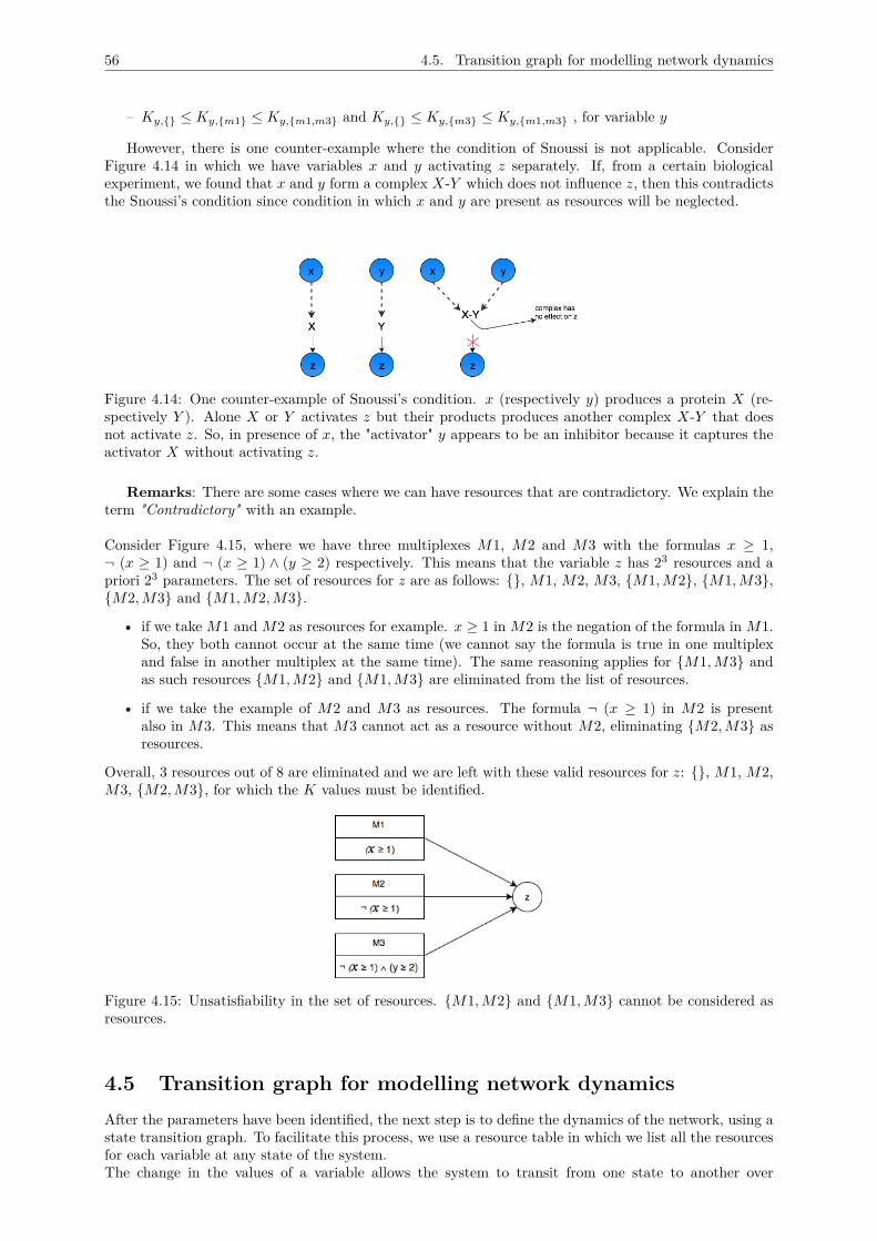
56 4.5. Transition graph for modelling network dynamics
– Ky,{} ≤ Ky,{m1} ≤ Ky,{m1,m3} and Ky,{} ≤ Ky,{m3} ≤ Ky,{m1,m3} , for variable y
However, there is one counter-example where the condition of Snoussi is not applicable. ConsiderFigure 4.14 in which we have variables x and y activating z separately. If, from a certain biologicalexperiment, we found that x and y form a complex X-Y which does not influence z, then this contradictsthe Snoussi’s condition since condition in which x and y are present as resources will be neglected.
Figure 4.14: One counter-example of Snoussi’s condition. x (respectively y) produces a protein X (re-spectively Y ). Alone X or Y activates z but their products produces another complex X-Y that doesnot activate z. So, in presence of x, the "activator" y appears to be an inhibitor because it captures theactivator X without activating z.
Remarks: There are some cases where we can have resources that are contradictory. We explain theterm "Contradictory" with an example.
Consider Figure 4.15, where we have three multiplexes M1, M2 and M3 with the formulas x ≥ 1,¬ (x ≥ 1) and ¬ (x ≥ 1) ∧ (y ≥ 2) respectively. This means that the variable z has 23 resources and apriori 23 parameters. The set of resources for z are as follows: {}, M1, M2, M3, {M1,M2}, {M1,M3},{M2,M3} and {M1,M2,M3}.
• if we take M1 and M2 as resources for example. x ≥ 1 in M2 is the negation of the formula in M1.So, they both cannot occur at the same time (we cannot say the formula is true in one multiplexand false in another multiplex at the same time). The same reasoning applies for {M1,M3} andas such resources {M1,M2} and {M1,M3} are eliminated from the list of resources.
• if we take the example of M2 and M3 as resources. The formula ¬ (x ≥ 1) in M2 is presentalso in M3. This means that M3 cannot act as a resource without M2, eliminating {M2,M3} asresources.
Overall, 3 resources out of 8 are eliminated and we are left with these valid resources for z: {}, M1, M2,M3, {M2,M3}, for which the K values must be identified.
Figure 4.15: Unsatisfiability in the set of resources. {M1,M2} and {M1,M3} cannot be considered asresources.
4.5 Transition graph for modelling network dynamicsAfter the parameters have been identified, the next step is to define the dynamics of the network, using astate transition graph. To facilitate this process, we use a resource table in which we list all the resourcesfor each variable at any state of the system.The change in the values of a variable allows the system to transit from one state to another over
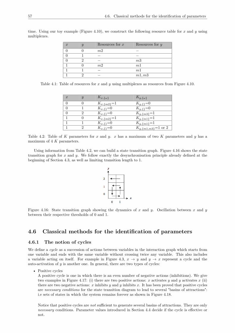
57 4.6. Classical methods for the identification of parameters
time. Using our toy example (Figure 4.10), we construct the following resource table for x and y usingmultiplexes.
x y Resources for x Resources for y0 0 m2 −0 1 − −0 2 − m31 0 m2 m11 1 − m11 2 − m1,m3
Table 4.1: Table of resources for x and y using multiplexes as resources from Figure 4.10.
x y Kx,{ω} Ky,{ω}
0 0 Kx,{m2}=1 Ky,{}=00 1 Kx,{}=0 Ky,{}=00 2 Kx,{}=0 Ky,{m3}=11 0 Kx,{m2}=1 Ky,{m1}=11 1 Kx,{}=0 Ky,{m1}=11 2 Kx,{}=0 Ky,{m1,m3}=1 or 2
Table 4.2: Table of K parameters for x and y. x has a maximum of two K parameters and y has amaximum of 4 K parameters.
Using information from Table 4.2, we can build a state transition graph. Figure 4.16 shows the statetransition graph for x and y. We follow exactly the desynchronisation principle already defined at thebeginning of Section 4.3, as well as limiting transition length to 1.
Figure 4.16: State transition graph showing the dynamics of x and y. Oscillation between x and ybetween their respective thresholds of 0 and 1.
4.6 Classical methods for the identification of parameters
4.6.1 The notion of cyclesWe define a cycle as a succession of actions between variables in the interaction graph which starts fromone variable and ends with the same variable without crossing twice any variable. This also includesa variable acting on itself. For example in Figure 4.3, x → y and y → x represent a cycle and theauto-activation of y is another one. In general, there are two types of cycles:
• Positive cyclesA positive cycle is one in which there is an even number of negative actions (inhibitions). We givetwo examples in Figure 4.17: (i) there are two positive actions: x activates y and y activates x (ii)there are two negative actions: x inhibits y and y inhibits x. It has been proved that positive cyclesare necessary conditions for the state transition diagram to lead to several "basins of attractions":i.e sets of states in which the system remains forever as shown in Figure 4.18.
Notice that positive cycles are not sufficient to generate several basins of attractions. They are onlynecessary conditions. Parameter values introduced in Section 4.4 decide if the cycle is effective ornot.
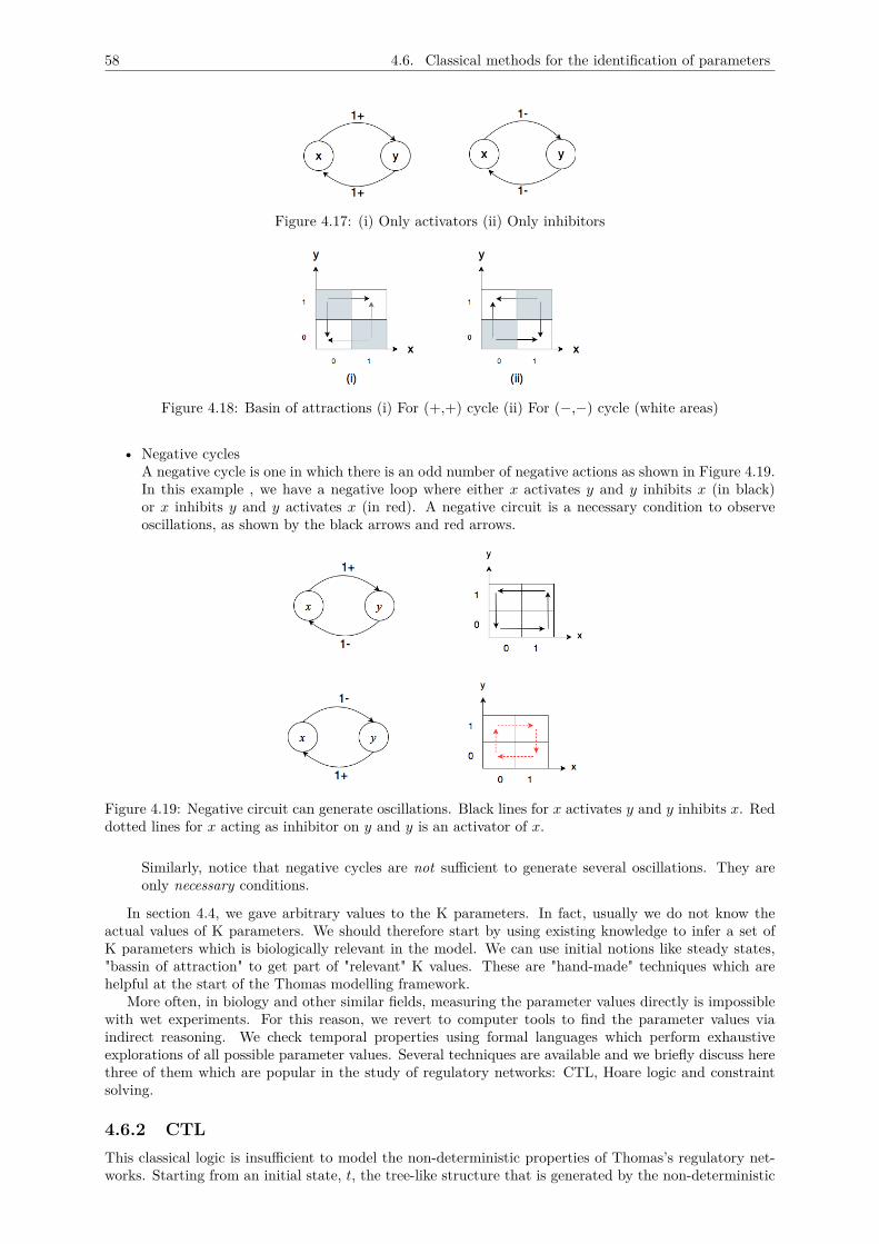
58 4.6. Classical methods for the identification of parameters
Figure 4.17: (i) Only activators (ii) Only inhibitors
Figure 4.18: Basin of attractions (i) For (+,+) cycle (ii) For (−,−) cycle (white areas)
• Negative cyclesA negative cycle is one in which there is an odd number of negative actions as shown in Figure 4.19.In this example , we have a negative loop where either x activates y and y inhibits x (in black)or x inhibits y and y activates x (in red). A negative circuit is a necessary condition to observeoscillations, as shown by the black arrows and red arrows.
Figure 4.19: Negative circuit can generate oscillations. Black lines for x activates y and y inhibits x. Reddotted lines for x acting as inhibitor on y and y is an activator of x.
Similarly, notice that negative cycles are not sufficient to generate several oscillations. They areonly necessary conditions.
In section 4.4, we gave arbitrary values to the K parameters. In fact, usually we do not know theactual values of K parameters. We should therefore start by using existing knowledge to infer a set ofK parameters which is biologically relevant in the model. We can use initial notions like steady states,"bassin of attraction" to get part of "relevant" K values. These are "hand-made" techniques which arehelpful at the start of the Thomas modelling framework.
More often, in biology and other similar fields, measuring the parameter values directly is impossiblewith wet experiments. For this reason, we revert to computer tools to find the parameter values viaindirect reasoning. We check temporal properties using formal languages which perform exhaustiveexplorations of all possible parameter values. Several techniques are available and we briefly discuss herethree of them which are popular in the study of regulatory networks: CTL, Hoare logic and constraintsolving.
4.6.2 CTLThis classical logic is insufficient to model the non-deterministic properties of Thomas’s regulatory net-works. Starting from an initial state, t, the tree-like structure that is generated by the non-deterministic
59 4.6. Classical methods for the identification of parameters
possibilities that exists for transiting between states better captures this non-deterministic characteristic.Going from one state to another can have several possibilities based on the set of resources (and thevalues of the K parameters) at that particular moment. There are certain biological properties thatare observable in-vitro or in-vivo over time for example, the oscillatory properties of certain biologicalentity, the occurence of one event following another one and so on, and these can be easily captured usingtemporal logic.
Many temporal logic variants are available (LTL, CTL, CTL* and so on) and we will use CTL be-cause it is a suitably branching time logic with efficient model checking capabilities [114, 115, 116]. Asshown in Chapter 3, in addition to using propositional logic for expressing biological properties, CTLalways uses two additional operators: a quantifier operator followed by a temporal operator. By givingcertain initial condition(s) and the property or list of properties we want to observe (written in a well-formed CTL formula), SMBioNet enumerates all the K parameter values which satisfy these temporalspecifications. This is handled properly via model checkers like NuSMV.
The verification of these CTL properties is done using a software platform which helps the modellerto give as input a well-formed CTL formula (and the state transition graph) and returns whether theformula is satisfied or not. Using our parameter identification tool SMBIoNet (in which model checkingis integrated), SMBioNet takes as input the CTL formula and traces systematically all the credible Kparameters which satisfies the given CTL property. If some K parameters are known, we specify themin the software and we let the model checker enumerates the set of remaining missing K parameters.
For our toy example of Figure 4.3, let us suppose we do not know the K parameters for x and y,and there is some observation that x and y oscillate. This additional knowledge of oscillations allows usto translate it into the CTL formula: (x = 0 ⇒ AF (x = 1)) ∧ ((x = 1 ⇒ AF (x = 0)). SMBioNet usesthis formula and the boundary of each variable ([0,1] for x and [0,1] for y) to enumerate all K parametersthat will satisfy this CTL formula.
In Figure 4.3, if the biologists have observed that x and y oscillate when y < 2, then we can trans-late this knowledge in CTL :
(y = 0 ⇒ AF(y = 1)
(y = 1 ⇒ AF(y = 0)
If the conditions of Snoussi are verified, then SMBioNet determine the following K parameters:
For x :
Kx = 0Kx,y = 1
For y :
Ky = 0Ky,x = 1, 2Ky,y = 0, 1, 2Ky,xy = 1, 2
And this coherent with Table 4.2 for example.We have use CTL extensively to enumerate all the 100 K parameters for our metabolic model enriched
by a bibliographic knowledge from biological literature.
4.6.3 Hoare LogicHere, we discuss a different approach from computer science based on Hoare logic and its associatedweakest precondition calculus that generates constraints on these parameters. Hoare logic was initiatedby Flyod and Hoare [117], to provide a proof system for imperative program correctness. A program isconsidered correct if it produces the expected output based on the inputs. In [112], Bernot et al showedthat this proof technique, if "genetically modified", can find interesting applications in systems biology.
60 4.6. Classical methods for the identification of parameters
Most of the time, biological experiments (with certain initial conditions) offer the possibility for molec-ular biologists to observe some traces (transcriptomic or proteomic levels) of the system with a certainexpected observable outputs. This scenario is almost identical to extracting programs from experiments.A computer program takes a certain input(s), processes the inputs to produce a given set of output(s).Using expected properties of the outputs, if we go backward by using the changes in the variables dur-ing the program, we can deduce the preconditions before the program executed to get these expectedproperties of the outputs. In the "genetically modified" Hoare logic, this process can be written as a triple:
{Initial conditions} Biological−traces−−−−−−−−−−−−→ {Observed final properties},
whose equivalent is expressable mathematically as a Hoare triple [111]:
{P} S {Q}
where P represents a set of preconditions, Q a set of postconditions and S the set of traces during theexperiment.
Hoare logic avoids building the complete state graph by working only on the traces, the observablefinal state and putting constraints on K parameters. In doing so, it provides a fast computation time tofind the set of consistent parameters. Next, we give some formal definitions helpful to write the tripleproperties of Hoare.
Considering any value of v ∈ V in a regulatory network, v can evolve only in two conditions:
• v increases if ηv < Kv,ω; that is η′v = ηv + 1 (where ηv represents the current state of v and η′
v
represents the next state). In the trace, this is represented by v+, that is v is attracted towards ahigher value.
• v decreases if ηv > Kv,ω; that is η′v = ηv - 1. In the trace, this is represented by v−, that is v isattracted towards a lower value.
Definition 4.6.1. (Trace specifications of discrete regulatory networks) − Let N = (V,M,E,K) be aregulatory network. The set of trace specifications for N is inductively defined by:
• For each v ∈ V and n ∈ [0, bv], the expressions v+, v− and v := n are atomic trace specifications(respectively increase, decrease or assignment to a specific value n during experiment).
• If e is an assertion for N , then the expression assert(e) is an atomic trace specification (see [112]for a complete syntax of the assertion).
• ε is called the empty trace.
• Several traces can be grouped sequentially together using quantifiers ∀ and ∃.
We reuse the toy example in Figure 4.4 to illustrate how Hoare logic facilitates the identification ofparameters for the variables x and y. Assuming that following some experiences carried out by biologists,we found the following traces and output:{ }
x+; y+;x−; y −{x = 0y = 0
}Starting from the output of x = 0 and y = 0, we proceed backward step by step using the traces to
determine the initial values of x and y. Since there are 4 observations, we have four steps as follows:
• Before the last observation, y decreased (y−), therefore we must have: y = 1 and x = 0, andmoreover (the genetically modified part) because y has decreased, Ky,ω1 < y. At this point, x = 0and y = 1 thus the set of resources of y is ω1 = {} (because x = 0). So, we get x = 0 ∧ y = 1 ∧ Ky
< y, which is equivalent to x = 0∧ y = 1∧Ky = 0. We will similar explanations for the remainingthree observations.
• Next, in the trace, we have x− which means y = 1 and x = 1, and because x has decreased, thismeans Kx,ω2 < x. At this point, x = 1 and y = 1, and the set of resources of x is ω = {}, we getx = 1 ∧ y = 1 and Kx < x, which is equivalent to x = 1 ∧ y = 1 ∧Kx = 0 ∧Ky = 0.
61 4.7. Conclusion of the chapter
• Next, in the trace, we have y+ which gives us y = 0, x = 1 and moreover since y has increasedKy,ω3 > y. At this point, x = 1, y = 0, then the set of resources for y is {x}. So, we getx = 1 ∧ y = 0 ∧Ky,ω3 > 0 (Ky,x > 0).
• Last, we have x+ observed in the trace from which we must have x = 0 and y = 0, and more-over since x has increased Kx,ω4 > x. At this point, with x = 0 and y = 0, the set of resourcesfor x is ω4={y}. So, we get x = 0∧y = 0∧Kx,y > x, which is equivalent to x = 0, y = 0 and Kx = 1.
Remark : We have the same results as in CTL and this is normal since we wanted to verify theoscillation of x and y.
In this thesis, we finally have been fortunate enough to identify all the 100 K parameters of our modeldirectly from the basis of biological literature and CTL formulas. It was not necessary to use Hoare logic.This technique is suitable in the long run if there are many unknown parameters and we tag it so that wecan consider it in any future endeavours. In the general case, the constraints can be more complicatedand this is where the use of Constraint solving is important. The next section gives a small rapid flavourof what constraint solving does.
4.6.4 Constraint SolvingConstraint solving is a computer science approach to find values of variables that satisfy some relationshipsbetween variables in the form of constraints [108]. It consists of the following:
• A finite set of variables which stores the solution. For our example, this set includes {x, y,Kx,Kx,y,Ky,Ky,x,Ky,y,Ky,xy}.
• A set of discrete values known as domain for each variable. In our example, we have the followingdomain for the variables: x ∈ {0, 1}, as well as all the kinetic parameters of x, and y ∈ {0, 1, 2} aswell as all its kinetic parameters.
• A finite set of constraints which will help in finding the solution (in our case finding the K param-eters).
Two problem solving domains where constraint solving have proved to be successful are: boolean andlinear domain. In the boolean domain, a variable can be true or false. In the linear form, the relationshipscan be expressed as systems of equations and inequalities (for example Kx,y > 0).
4.7 Conclusion of the chapterIn this chapter, we have covered the framework of Réné Thomas well adapted for the regulations ofbiological networks with a qualitative vision. Our study is on the regulation of the energy and biomassmetabolism for which formal qualitative frameworks are the best suited formalisms.
We have presented two versions of the Thomas’s framework: the classical one (without multiplexes)and one with multiplexes (less K parameters). The name of multiplexes in the second improved versionallowed an easy interpretation of the type of interactions between variables. We will see in Chapter 5 howand when we choose between a variable and a multiplex. In the discrete formalism of R.Thomas, the val-ues of the kinetic parameters are normally small integer values for which the identification is easier thanthe classical differential equations (where the values are real). Nevertheless, the identification of thesekinetic parameters, even if integers, represent the main difficulties in the modelling of biological networks.
With R. Thomas approach, biological networks are represented using state transition graphs and thereforebenefit from formal methods. We have three formal methods: CTL, Hoare logic (modified version) andconstraint programming. In all three cases, the biological knowledge from experiences are fundamentalfor either writing CTL formulas, translating into Hoare Triples or expressing in terms of constraints.
In the particular case of our model and the high abstraction used, all the K parameters have beenidentified using information from biological literature. But, we have used CTL to validate the set ofvalues of the K parameters.
CHAPTER 5A METHODOLOGY FOR THOMAS
MODEL DESIGN
IntroductionThe activities for the modelling of dynamic networks have some similarities with the activities for theconception of a software in software engineering. In software engineering, a panoply of useful method-ologies (software life cycle models, rapid prototyping, Agile methodologies [119]) are used. Traditionally,to achieve good software quality, methodologies have been instrumental in the software development lifecycle and for good project management for decades. For example, the V-model in software development(which is inspired from the general V-model in technology) has a set of procedures starting from require-ments analysis of a software to its validation by end users. In requirements analysis, the needs of the userare collected (what is the problem that is being addressed). This gives an exhaustive description of thesoftware expected set of functionalities. After this crucial step that defines what the software is supposedto do, the software design process starts in order to choose how the software will do. Successive stepsare often followed, depending on the size of the software : from 0 to several intermediate specificationsprogressively introducing "how solutions", and a last detailed specification containing all the main choices.The detailed specification contains modules that facilitate a multi-team development of the software. Thisdivision of tasks allows multiple developers to work on the problem. As each module is developed, theirunit testing can be done. Once this verification process is completed, modules are progressively integratedto make the whole software and integration testing is performed. At this stage, system testing is carriedout to assess the global functioning and the product is delivered to the client. A final step validates allthe functionalities with the initial set of objectives proposed by the user often called "functional test-ing". These rigorous steps make sure all the stakeholders sub products in the system life cycle are checked.
In general, a methodology can be described as a blueprint containing well-defined procedures to achievea particular task. Many advantages exist when using a methodological approach: smooth teamwork on acollaborative project, a faster development lifecycle of a given product, reverting to any particular step incase something goes wrong, and the possibility to apply the methodology to a range of types and sizes ofproblems. A well chosen methodology strongly helps to build a product of good quality with respect tothe user specifications, which are initially developed before designing the model. We are going to adopta similar strategy, which starts with user requirements followed by development and testing.
We propose a full methodology in this chapter which has been successful in the design of our coarse-grained model of the regulation of the energy and biomass metabolism network. All its steps are ap-plicable to any other network using the Thomas framework. In this methodology, we have exploited tothe maximum the particularities of the Thomas’ framework namely the notion of thresholds, the precisemeaning of parameters, the ability to perform intensive model checking and simulations. In this chapter,we present a global view of the main steps of the methodology:
1. The opening step aims at better defining the biological problem into consideration, leading to aninventory of variables we need to make explicit. We also provide "types" to variables, depending onthe biological context.
2. In step 2, we extract the minimum number of threshold values for each variable by asking thebiologist the exhaustive set of targets of each variable. The variables may be boolean or multivalued,and the order between thresholds is validated with biological justifications from literature or fromexperimental data. This is a delicate step and sometimes requires revising the variables, and thecontext, to get sensible information at the proper abstract level.
62
63 5.1. Inventory of main variables
3. In biology, there exist many combined regulations which can co-exist and this is the objective ofstep 3 where we discuss how we deal with these regulations using multiplexes. Again here, thebiologist is central to be able to tell the biological importance of each multiplex and the formulasinvolved in it. At this stage, it stands to reason on the choice of the multiplex. Also, we decide if avariable is really needed or if it can simply be represented as a multiplex (in which case, the modelspares the state of a variable, which will facilitate further studies).
4. The importance of a validation matrix, inspired from the functional testing of the final validationstep in software engineering, is explained in step 4. The validation matrix is used to give themain behaviours that the model must exhibit according to biological knowledge. This matrix isdesigned before the identification of K parameters and as such it is constructed independently. Theproperties used in step 5 to identify the missing K parameters should be independent of this matrix.
5. The thorough identification of a maximum possible number of K parameters using biological knowl-edge for a given model is elaborated in step 5. For the remaining unknown K parameters, formaltechniques, like model checking and Hoare logic, are available to complete the set of parametervalues.
6. In step 6, we see the usefulness of simulations and how we get initial hints on the mathematicalmodel and whether those observations are possible with respect to the biological model. At the sametime, we can extrapolate those observations and transform them into appropriate CTL formulaswhich can be validated using model checking tools (further explained in Chapter 6), participatingto the predictive capabilities of the model.
7. The last step of this methodology validates the model using the validation matrix. We use fair pathCTL to make sure all trajectories are treated equally and are reachable. This step is independentof the feasibility study in the previous step and as such is a way of validating known properties ina time-independent manner. If validation fails, one must backtrack and a careful analysis of thepossible reasons of invalidity helps to choose at which step one needs to backtrack.
The remainder of this chapter exactly follows these steps of the methodology.
5.1 Inventory of main variablesGenerally, in the design of any network, we must first construct a list of basic components making thenodes of the network. This is to make sure every sensible concept is incorporated in the design process.In a typical biological network, these components can take the form of proteins, genes or biological pro-cesses, and this is highly dependent on the problem under consideration, the biological hypotheses tocheck and more generally the discussions we have with the biologist. One must be careful to make achoice of variables as abstract as possible, in order to better capture the main causalities in the model.
At a particular point of time, in order to gain some new insights about the dynamics of the network, wemust introduce the external environment to which the network will be confronted. The integration of theenvironmental factors is helpful to simulate different scenarios and thus provides a more detailed viewabout the compatibility of the futur model with the biological system it represents. This gives a greatdeal of flexibility to the modeller, when validating the network in terms of which control variables canbe turned ON or OFF (signalling their presence/absence in the environment; for example, the presenceof oxygen to mimic aerobic respiration). These variables are called environmental or input variables.They can represent drugs, nutrients, growth factors and many alike. Input variables can also be multi-valued, for example, glucose intake can be low(0), normal(1) or in excess (2).
In this variable identification process, which is the starting point of the methodology, it may happenthat if the network is large, we are obliged to categorise the variables, more precisely than as "input vari-ables" vs "internal variables". The advantages are many-folds: each category can represent a topologicalinterest; for example cell compartments (cytoplasm or mitochondria), biological processes or a group ofproteins having similar cellular functions (for example enzymes). When tracing the interactions betweenthese variables in a graph, we can use different colours to represent these variable types.
At the end of this step, we have an overview of all the variables and how they abstract a given bio-logical function or molecule. The interdependency between all the variables results in an intermediateand informal graph. Upon consultation with the biologist, this graph helps us to make sure that we have
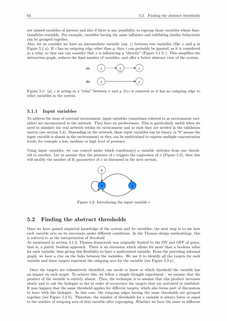
64 5.2. Finding the abstract thresholds
not missed variables of interest and also if there is any possibility to regroup those variables whose func-tionalities resemble. For example, variables having the same influence and exhibiting similar behaviourscan be grouped together.Also, let us consider we have an intermediate variable (say z) between two variables (like x and y inFigure 5.1 a). If z has no outgoing edge other than y, then z can probably be ignored, as it is consideredas a relay, so that one can consider that x is influencing y "directly" (Figure 5.1 b ). This simplifies theinteraction graph, reduces the final number of variables, and offer a better abstract view of the system.
Figure 5.1: (a) z is acting as a "relay" between x and y (b)z is removed as it has no outgoing edge toother variables in the system.
5.1.1 Input variablesTo address the issue of external environment, input variables (sometimes referred to as environment vari-ables) are incorporated in the network. They have no predecessors. This is particularly useful when weneed to simulate the real network within its environment and as such they are needed in the validationmatrix (see section 5.4). Depending on the network, these input variables can be binary (a "0" means theinput variable is absent in the environment) or they can be multivalued to express multiple concentrationlevels; for example a low, medium or high level of presence.
Using input variables, we can control under which condition(s) a variable switches from one thresh-old to another. Let us assume that the presence of c triggers the expression of x (Figure 5.2), then thiswill modify the number of K parameters of x as discussed in the next section.
Figure 5.2: Introducing the input variable c
5.2 Finding the abstract thresholdsOnce we have gained empirical knowledge of the system and its variables, the next step is to see howeach variable acts on its successors under different conditions. In the Thomas design methodology, thisis referred to as the interpretation of threshold.As mentioned in section 4.1.2, Thomas framework was originally limited to the ON and OFF of genes,that is, a purely boolean approach. There is an extension which allows for more than a boolean valuefor each variable; thus giving this flexibility to have a multivalued variable. From the preceding informalgraph, we have a clue on the links between the variables. We use it to identify all the targets for eachvariable and these targets represent the outgoing arcs for the variable (see Figure 5.3 a).
Once the targets are exhaustively identified, one needs to know at which threshold the variable hasan impact on each target. To achieve this, we follow a simple thought experiment : we assume that theproduct of the variable is entirely absent. Then, the technique is to assume that this product increasesslowly and to ask the biologist to list in order of occurrence the targets that are activated or inhibited.It may happen that the same threshold applies for different targets, which also forms part of discussionsto have with the biologist. In this case, the outgoing edges having the same thresholds are groupedtogether (see Figure 5.3 b). Therefore, the number of thresholds for a variable is always lower or equalto the number of outgoing arcs of that variable after regrouping. Whether we have the same or different
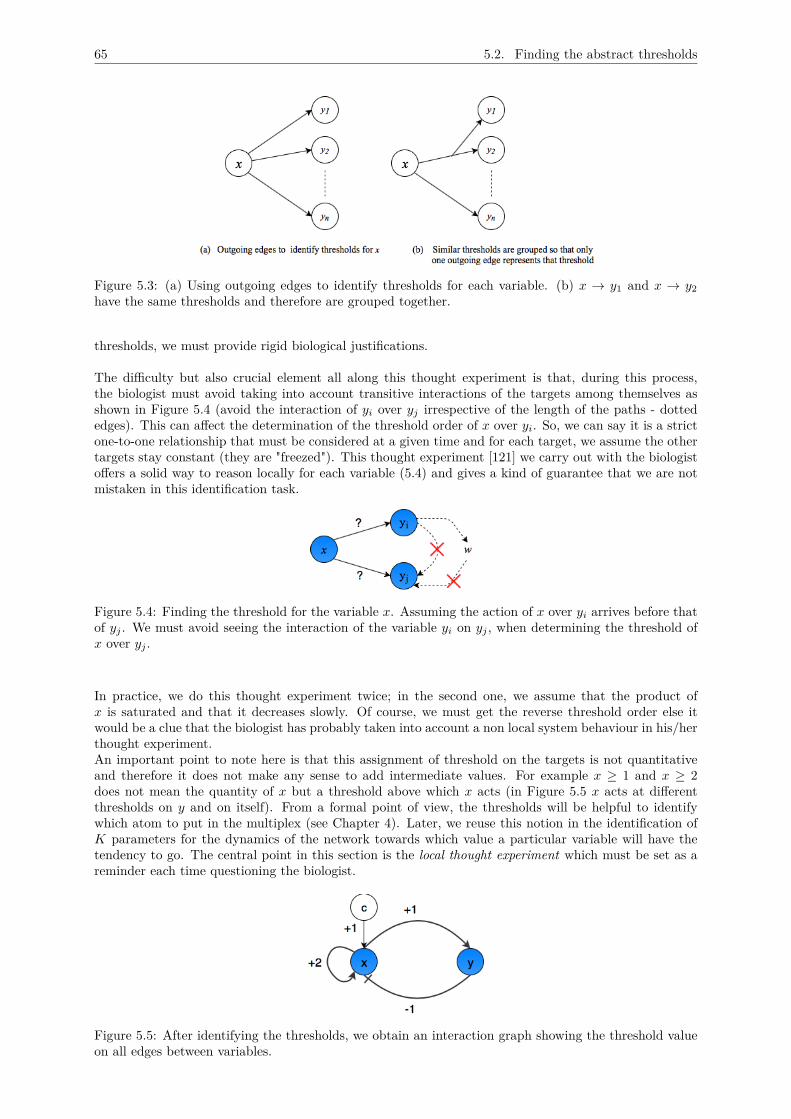
65 5.2. Finding the abstract thresholds
Figure 5.3: (a) Using outgoing edges to identify thresholds for each variable. (b) x → y1 and x → y2have the same thresholds and therefore are grouped together.
thresholds, we must provide rigid biological justifications.
The difficulty but also crucial element all along this thought experiment is that, during this process,the biologist must avoid taking into account transitive interactions of the targets among themselves asshown in Figure 5.4 (avoid the interaction of yi over yj irrespective of the length of the paths - dottededges). This can affect the determination of the threshold order of x over yi. So, we can say it is a strictone-to-one relationship that must be considered at a given time and for each target, we assume the othertargets stay constant (they are "freezed"). This thought experiment [121] we carry out with the biologistoffers a solid way to reason locally for each variable (5.4) and gives a kind of guarantee that we are notmistaken in this identification task.
Figure 5.4: Finding the threshold for the variable x. Assuming the action of x over yi arrives before thatof yj . We must avoid seeing the interaction of the variable yi on yj , when determining the threshold ofx over yj .
In practice, we do this thought experiment twice; in the second one, we assume that the product ofx is saturated and that it decreases slowly. Of course, we must get the reverse threshold order else itwould be a clue that the biologist has probably taken into account a non local system behaviour in his/herthought experiment.An important point to note here is that this assignment of threshold on the targets is not quantitativeand therefore it does not make any sense to add intermediate values. For example x ≥ 1 and x ≥ 2does not mean the quantity of x but a threshold above which x acts (in Figure 5.5 x acts at differentthresholds on y and on itself). From a formal point of view, the thresholds will be helpful to identifywhich atom to put in the multiplex (see Chapter 4). Later, we reuse this notion in the identification ofK parameters for the dynamics of the network towards which value a particular variable will have thetendency to go. The central point in this section is the local thought experiment which must be set as areminder each time questioning the biologist.
Figure 5.5: After identifying the thresholds, we obtain an interaction graph showing the threshold valueon all edges between variables.
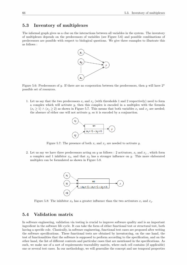
66 5.3. Inventory of multiplexes
5.3 Inventory of multiplexesThe informal graph gives us a clue on the interactions between all variables in the system. The inventoryof multiplexes depends on the predecessors of variables (see Figure 5.6) and possible combinations ofpredecessors are possible with respect to biological questions. We give three examples to illustrate thisas follows :
Figure 5.6: Predecessors of y. If there are no cooperation between the predecessors, then y will have 2n
possible set of resources.
1. Let us say that the two predecessors xi and xj (with thresholds 1 and 2 respectively) need to forma complex which will activate y, then this complex is encoded in a multiplex with the formula(xi ≥ 1) ∧ (xj ≥ 2) as shown in Figure 5.7. This means that both variables xi and xj are needed;the absence of either one will not activate y, so it is encoded by a conjunction.
Figure 5.7: The presence of both xi and xj are needed to activate y.
2. Let us say we have three predecessors acting on y as follows : 2 activators, xi and xj , which forma complex and 1 inhibitor xk, and that xk has a stronger influence on y. This more elaboratedmultiplex can be formulated as shown in Figure 5.8.
Figure 5.8: The inhibitor xk has a greater influence than the two activators xi and xj .
5.4 Validation matrixIn software engineering, validation via testing is crucial to improve software quality and is an importantingredient in the software life cycle. It can take the form of either functional test or structural test, bothhaving a specific role. Classically, in software engineering, functional test cases are proposed after writingthe software specifications. These functional tests are obtained by inventorying, on the one hand, thetest of functionalities that the software is supposed to perform according to the specification, and on theother hand, the list of different contexts and particular cases that are mentioned in the specifications. Assuch, we make use of a sort of requirements traceability matrix, where each cell contains (if applicable)one or several test cases. In our methodology, we will generalise the concept and use temporal properties
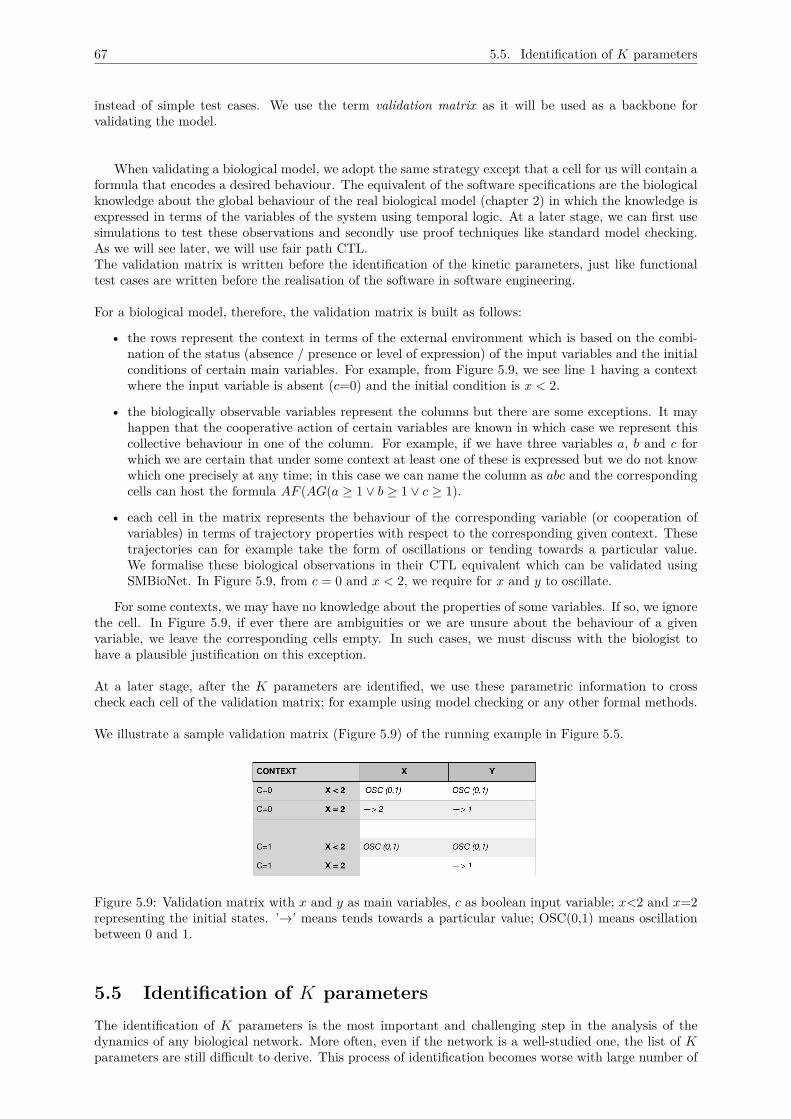
67 5.5. Identification of K parameters
instead of simple test cases. We use the term validation matrix as it will be used as a backbone forvalidating the model.
When validating a biological model, we adopt the same strategy except that a cell for us will contain aformula that encodes a desired behaviour. The equivalent of the software specifications are the biologicalknowledge about the global behaviour of the real biological model (chapter 2) in which the knowledge isexpressed in terms of the variables of the system using temporal logic. At a later stage, we can first usesimulations to test these observations and secondly use proof techniques like standard model checking.As we will see later, we will use fair path CTL.The validation matrix is written before the identification of the kinetic parameters, just like functionaltest cases are written before the realisation of the software in software engineering.
For a biological model, therefore, the validation matrix is built as follows:
• the rows represent the context in terms of the external environment which is based on the combi-nation of the status (absence / presence or level of expression) of the input variables and the initialconditions of certain main variables. For example, from Figure 5.9, we see line 1 having a contextwhere the input variable is absent (c=0) and the initial condition is x < 2.
• the biologically observable variables represent the columns but there are some exceptions. It mayhappen that the cooperative action of certain variables are known in which case we represent thiscollective behaviour in one of the column. For example, if we have three variables a, b and c forwhich we are certain that under some context at least one of these is expressed but we do not knowwhich one precisely at any time; in this case we can name the column as abc and the correspondingcells can host the formula AF (AG(a ≥ 1 ∨ b ≥ 1 ∨ c ≥ 1).
• each cell in the matrix represents the behaviour of the corresponding variable (or cooperation ofvariables) in terms of trajectory properties with respect to the corresponding given context. Thesetrajectories can for example take the form of oscillations or tending towards a particular value.We formalise these biological observations in their CTL equivalent which can be validated usingSMBioNet. In Figure 5.9, from c = 0 and x < 2, we require for x and y to oscillate.
For some contexts, we may have no knowledge about the properties of some variables. If so, we ignorethe cell. In Figure 5.9, if ever there are ambiguities or we are unsure about the behaviour of a givenvariable, we leave the corresponding cells empty. In such cases, we must discuss with the biologist tohave a plausible justification on this exception.
At a later stage, after the K parameters are identified, we use these parametric information to crosscheck each cell of the validation matrix; for example using model checking or any other formal methods.
We illustrate a sample validation matrix (Figure 5.9) of the running example in Figure 5.5.
Figure 5.9: Validation matrix with x and y as main variables, c as boolean input variable; x<2 and x=2representing the initial states. ’→’ means tends towards a particular value; OSC(0,1) means oscillationbetween 0 and 1.
5.5 Identification of K parametersThe identification of K parameters is the most important and challenging step in the analysis of thedynamics of any biological network. More often, even if the network is a well-studied one, the list of Kparameters are still difficult to derive. This process of identification becomes worse with large number of
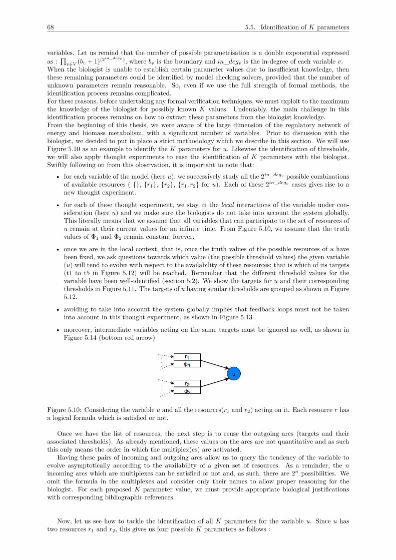
68 5.5. Identification of K parameters
variables. Let us remind that the number of possible parametrisation is a double exponential expressedas :
∏v∈V (bv + 1)(2in_degv ), where bv is the boundary and in_degv is the in-degree of each variable v.
When the biologist is unable to establish certain parameter values due to insufficient knowledge, thenthese remaining parameters could be identified by model checking solvers, provided that the number ofunknown parameters remain reasonable. So, even if we use the full strength of formal methods, theidentification process remains complicated.For these reasons, before undertaking any formal verification techniques, we must exploit to the maximumthe knowledge of the biologist for possibly known K values. Undeniably, the main challenge in thisidentification process remains on how to extract these parameters from the biologist knowledge.From the beginning of this thesis, we were aware of the large dimension of the regulatory network ofenergy and biomass metabolism, with a significant number of variables. Prior to discussion with thebiologist, we decided to put in place a strict methodology which we describe in this section. We will useFigure 5.10 as an example to identify the K parameters for u. Likewise the identification of thresholds,we will also apply thought experiments to ease the identification of K parameters with the biologist.Swiftly following on from this observation, it is important to note that:
• for each variable of the model (here u), we successively study all the 2in_degv possible combinationsof available resources ( {}, {r1}, {r2}, {r1, r2} for u). Each of these 2in_degv cases gives rise to anew thought experiment.
• for each of these thought experiment, we stay in the local interactions of the variable under con-sideration (here u) and we make sure the biologists do not take into account the system globally.This literally means that we assume that all variables that can participate to the set of resources ofu remain at their current values for an infinite time. From Figure 5.10, we assume that the truthvalues of Φ1 and Φ2 remain constant forever.
• once we are in the local context, that is, once the truth values of the possible resources of u havebeen fixed, we ask questions towards which value (the possible threshold values) the given variable(u) will tend to evolve with respect to the availability of these resources; that is which of its targets(t1 to t5 in Figure 5.12) will be reached. Remember that the different threshold values for thevariable have been well-identified (section 5.2). We show the targets for u and their correspondingthresholds in Figure 5.11. The targets of u having similar thresholds are grouped as shown in Figure5.12.
• avoiding to take into account the system globally implies that feedback loops must not be takeninto account in this thought experiment, as shown in Figure 5.13.
• moreover, intermediate variables acting on the same targets must be ignored as well, as shown inFigure 5.14 (bottom red arrow)
Figure 5.10: Considering the variable u and all the resources(r1 and r2) acting on it. Each resource r hasa logical formula which is satisfied or not.
Once we have the list of resources, the next step is to reuse the outgoing arcs (targets and theirassociated thresholds). As already mentioned, these values on the arcs are not quantitative and as suchthis only means the order in which the multiplex(es) are activated.
Having these pairs of incoming and outgoing arcs allow us to query the tendency of the variable toevolve asymptotically according to the availability of a given set of resources. As a reminder, the nincoming arcs which are multiplexes can be satisfied or not and, as such, there are 2n possibilities. Weomit the formula in the multiplexes and consider only their names to allow proper reasoning for thebiologist. For each proposed K parameter value, we must provide appropriate biological justificationswith corresponding bibliographic references.
Now, let us see how to tackle the identification of all K parameters for the variable u. Since u hastwo resources r1 and r2, this gives us four possible K parameters as follows :
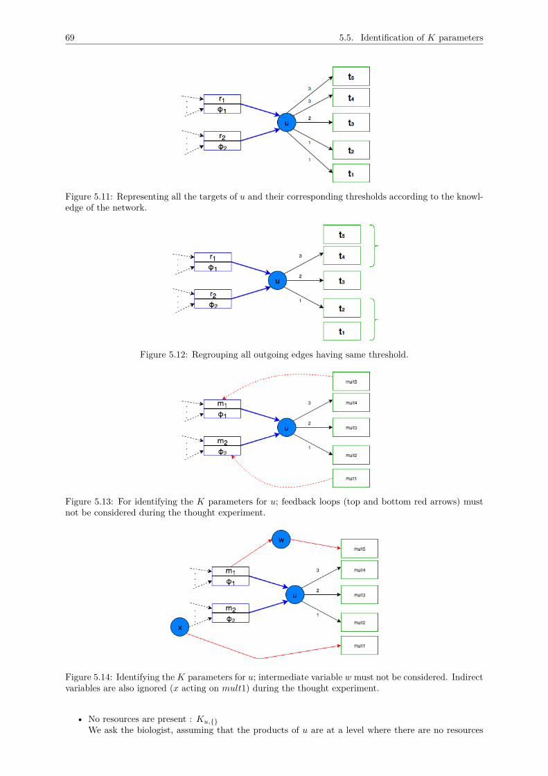
69 5.5. Identification of K parameters
Figure 5.11: Representing all the targets of u and their corresponding thresholds according to the knowl-edge of the network.
Figure 5.12: Regrouping all outgoing edges having same threshold.
Figure 5.13: For identifying the K parameters for u; feedback loops (top and bottom red arrows) mustnot be considered during the thought experiment.
Figure 5.14: Identifying the K parameters for u; intermediate variable w must not be considered. Indirectvariables are also ignored (x acting on mult1) during the thought experiment.
• No resources are present : Ku,{}We ask the biologist, assuming that the products of u are at a level where there are no resources
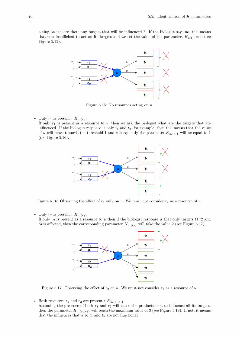
70 5.5. Identification of K parameters
acting on u : are there any targets that will be influenced ?. If the biologist says no, this meansthat u is insufficient to act on its targets and we set the value of the parameter, Ku,{} = 0 (seeFigure 5.15).
Figure 5.15: No resources acting on u.
• Only r1 is present : Ku,{r1}If only r1 is present as a resource to u, then we ask the biologist what are the targets that areinfluenced. If the biologist response is only t1 and t2, for example, then this means that the valueof u will move towards the threshold 1 and consequently the parameter Ku,{r1} will be equal to 1(see Figure 5.16).
Figure 5.16: Observing the effect of r1 only on u. We must not consider r2 as a resource of u.
• Only r2 is present : Ku,{r2}If only r2 is present as a resource to u then if the biologist response is that only targets t1,t2 andt3 is affected, then the corresponding parameter Ku,{r2} will take the value 2 (see Figure 5.17).
Figure 5.17: Observing the effect of r2 on u. We must not consider r1 as a resource of u.
• Both resources r1 and r2 are present : Ku,{r1,r2}Assuming the presence of both r1 and r2 will cause the products of u to influence all its targets,then the parameter Ku,{r1,r2} will reach the maximum value of 3 (see Figure 5.18). If not, it meansthat the influences that u to t4 and t5 are not functional.
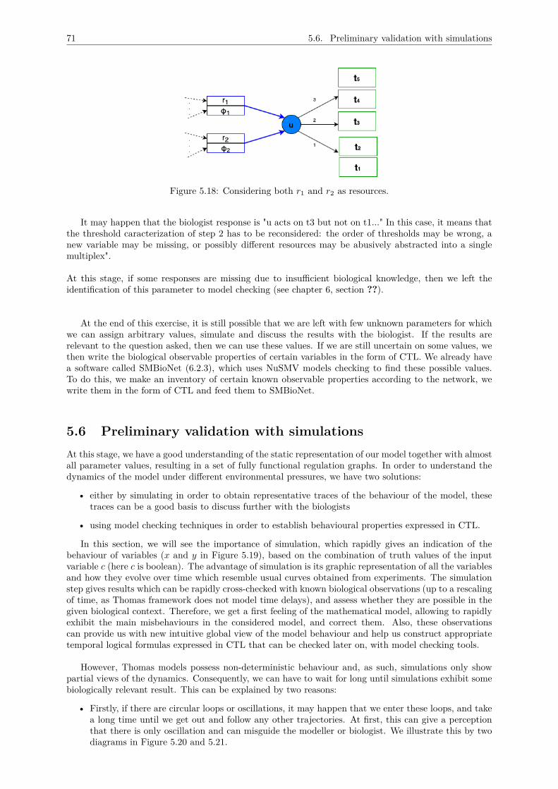
71 5.6. Preliminary validation with simulations
Figure 5.18: Considering both r1 and r2 as resources.
It may happen that the biologist response is "u acts on t3 but not on t1..." In this case, it means thatthe threshold caracterization of step 2 has to be reconsidered: the order of thresholds may be wrong, anew variable may be missing, or possibly different resources may be abusively abstracted into a singlemultiplex".
At this stage, if some responses are missing due to insufficient biological knowledge, then we left theidentification of this parameter to model checking (see chapter 6, section ??).
At the end of this exercise, it is still possible that we are left with few unknown parameters for whichwe can assign arbitrary values, simulate and discuss the results with the biologist. If the results arerelevant to the question asked, then we can use these values. If we are still uncertain on some values, wethen write the biological observable properties of certain variables in the form of CTL. We already havea software called SMBioNet (6.2.3), which uses NuSMV models checking to find these possible values.To do this, we make an inventory of certain known observable properties according to the network, wewrite them in the form of CTL and feed them to SMBioNet.
5.6 Preliminary validation with simulationsAt this stage, we have a good understanding of the static representation of our model together with almostall parameter values, resulting in a set of fully functional regulation graphs. In order to understand thedynamics of the model under different environmental pressures, we have two solutions:
• either by simulating in order to obtain representative traces of the behaviour of the model, thesetraces can be a good basis to discuss further with the biologists
• using model checking techniques in order to establish behavioural properties expressed in CTL.
In this section, we will see the importance of simulation, which rapidly gives an indication of thebehaviour of variables (x and y in Figure 5.19), based on the combination of truth values of the inputvariable c (here c is boolean). The advantage of simulation is its graphic representation of all the variablesand how they evolve over time which resemble usual curves obtained from experiments. The simulationstep gives results which can be rapidly cross-checked with known biological observations (up to a rescalingof time, as Thomas framework does not model time delays), and assess whether they are possible in thegiven biological context. Therefore, we get a first feeling of the mathematical model, allowing to rapidlyexhibit the main misbehaviours in the considered model, and correct them. Also, these observationscan provide us with new intuitive global view of the model behaviour and help us construct appropriatetemporal logical formulas expressed in CTL that can be checked later on, with model checking tools.
However, Thomas models possess non-deterministic behaviour and, as such, simulations only showpartial views of the dynamics. Consequently, we can have to wait for long until simulations exhibit somebiologically relevant result. This can be explained by two reasons:
• Firstly, if there are circular loops or oscillations, it may happen that we enter these loops, and takea long time until we get out and follow any other trajectories. At first, this can give a perceptionthat there is only oscillation and can misguide the modeller or biologist. We illustrate this by twodiagrams in Figure 5.20 and 5.21.
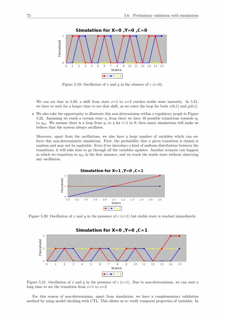
72 5.6. Preliminary validation with simulations
Figure 5.19: Oscillation of x and y in the absence of c (c=0).
We can see that in 5.20, a shift from state x=1 to x=2 reaches stable state instantly. In 5.21,we have to wait for a longer time to see that shift, as we enter the loop for both x(0,1) and y(0,1).
• We also take the opportunity to illustrate this non-determinism within a regulatory graph in Figure5.22. Assuming we reach a certain state η, from there we have 10 possible transitions towards η1to η10. We assume there is a loop from ηi to η for i=1 to 9; then many simulations will make usbelieve that the system always oscillates.
Moreover, apart from the oscillations, we also have a large number of variables which can en-force this non-deterministic simulation. First, the probability that a given transition is chosen israndom and may not be equitable. Even if we introduce a kind of uniform distribution between thetransitions, it will take time to go through all the variables updates. Another scenario can happenin which we transition to η10 in the first instance, and we reach the stable state without observingany oscillation.
Figure 5.20: Oscillation of x and y in the presence of c (c=1) but stable state is reached immediately.
Figure 5.21: Oscillation of x and y in the presence of c (c=1). Due to non-determinism, we can wait along time to see the transition from x=1 to x=2
For this reason of non-determinism, apart from simulation, we have a complementary validationmethod by using model checking with CTL. This allows us to verify temporal properties of variables. In
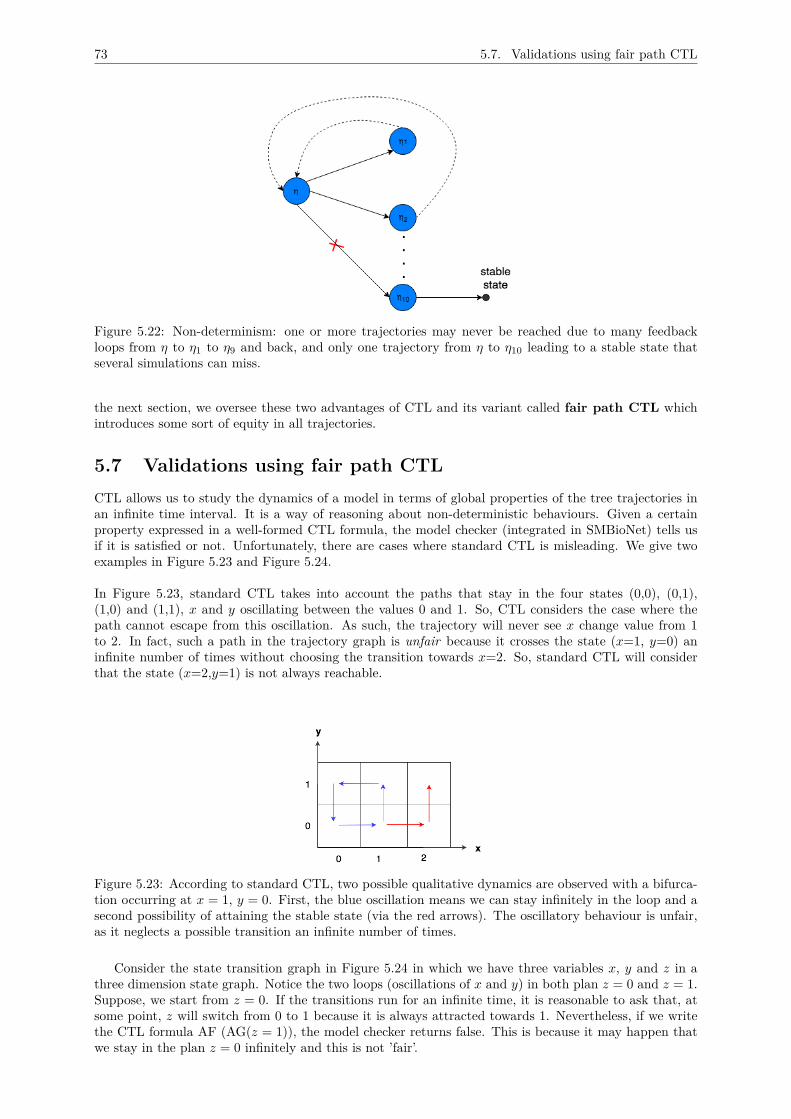
73 5.7. Validations using fair path CTL
Figure 5.22: Non-determinism: one or more trajectories may never be reached due to many feedbackloops from η to η1 to η9 and back, and only one trajectory from η to η10 leading to a stable state thatseveral simulations can miss.
the next section, we oversee these two advantages of CTL and its variant called fair path CTL whichintroduces some sort of equity in all trajectories.
5.7 Validations using fair path CTLCTL allows us to study the dynamics of a model in terms of global properties of the tree trajectories inan infinite time interval. It is a way of reasoning about non-deterministic behaviours. Given a certainproperty expressed in a well-formed CTL formula, the model checker (integrated in SMBioNet) tells usif it is satisfied or not. Unfortunately, there are cases where standard CTL is misleading. We give twoexamples in Figure 5.23 and Figure 5.24.
In Figure 5.23, standard CTL takes into account the paths that stay in the four states (0,0), (0,1),(1,0) and (1,1), x and y oscillating between the values 0 and 1. So, CTL considers the case where thepath cannot escape from this oscillation. As such, the trajectory will never see x change value from 1to 2. In fact, such a path in the trajectory graph is unfair because it crosses the state (x=1, y=0) aninfinite number of times without choosing the transition towards x=2. So, standard CTL will considerthat the state (x=2,y=1) is not always reachable.
Figure 5.23: According to standard CTL, two possible qualitative dynamics are observed with a bifurca-tion occurring at x = 1, y = 0. First, the blue oscillation means we can stay infinitely in the loop and asecond possibility of attaining the stable state (via the red arrows). The oscillatory behaviour is unfair,as it neglects a possible transition an infinite number of times.
Consider the state transition graph in Figure 5.24 in which we have three variables x, y and z in athree dimension state graph. Notice the two loops (oscillations of x and y) in both plan z = 0 and z = 1.Suppose, we start from z = 0. If the transitions run for an infinite time, it is reasonable to ask that, atsome point, z will switch from 0 to 1 because it is always attracted towards 1. Nevertheless, if we writethe CTL formula AF (AG(z = 1)), the model checker returns false. This is because it may happen thatwe stay in the plan z = 0 infinitely and this is not ’fair’.
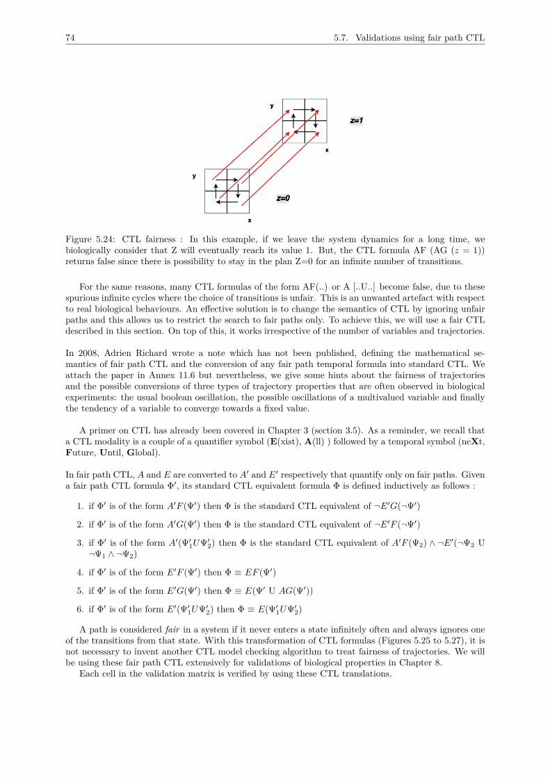
74 5.7. Validations using fair path CTL
Figure 5.24: CTL fairness : In this example, if we leave the system dynamics for a long time, webiologically consider that Z will eventually reach its value 1. But, the CTL formula AF (AG (z = 1))returns false since there is possibility to stay in the plan Z=0 for an infinite number of transitions.
For the same reasons, many CTL formulas of the form AF(..) or A [..U..] become false, due to thesespurious infinite cycles where the choice of transitions is unfair. This is an unwanted artefact with respectto real biological behaviours. An effective solution is to change the semantics of CTL by ignoring unfairpaths and this allows us to restrict the search to fair paths only. To achieve this, we will use a fair CTLdescribed in this section. On top of this, it works irrespective of the number of variables and trajectories.
In 2008, Adrien Richard wrote a note which has not been published, defining the mathematical se-mantics of fair path CTL and the conversion of any fair path temporal formula into standard CTL. Weattach the paper in Annex 11.6 but nevertheless, we give some hints about the fairness of trajectoriesand the possible conversions of three types of trajectory properties that are often observed in biologicalexperiments: the usual boolean oscillation, the possible oscillations of a multivalued variable and finallythe tendency of a variable to converge towards a fixed value.
A primer on CTL has already been covered in Chapter 3 (section 3.5). As a reminder, we recall thata CTL modality is a couple of a quantifier symbol (E(xist), A(ll) ) followed by a temporal symbol (neXt,Future, Until, Global).
In fair path CTL, A and E are converted to A′ and E′ respectively that quantify only on fair paths. Givena fair path CTL formula Φ′, its standard CTL equivalent formula Φ is defined inductively as follows :
1. if Φ′ is of the form A′F (Ψ′) then Φ is the standard CTL equivalent of ¬E′G(¬Ψ′)
2. if Φ′ is of the form A′G(Ψ′) then Φ is the standard CTL equivalent of ¬E′F (¬Ψ′)
3. if Φ′ is of the form A′(Ψ′1UΨ′2) then Φ is the standard CTL equivalent of A′F (Ψ2) ∧ ¬E′(¬Ψ2 U¬Ψ1 ∧ ¬Ψ2)
4. if Φ′ is of the form E′F (Ψ′) then Φ ≡ EF (Ψ′)
5. if Φ′ is of the form E′G(Ψ′) then Φ ≡ E(Ψ′ U AG(Ψ′))
6. if Φ′ is of the form E′(Ψ′1UΨ′2) then Φ ≡ E(Ψ′1UΨ′2)
A path is considered fair in a system if it never enters a state infinitely often and always ignores oneof the transitions from that state. With this transformation of CTL formulas (Figures 5.25 to 5.27), it isnot necessary to invent another CTL model checking algorithm to treat fairness of trajectories. We willbe using these fair path CTL extensively for validations of biological properties in Chapter 8.
Each cell in the validation matrix is verified by using these CTL translations.
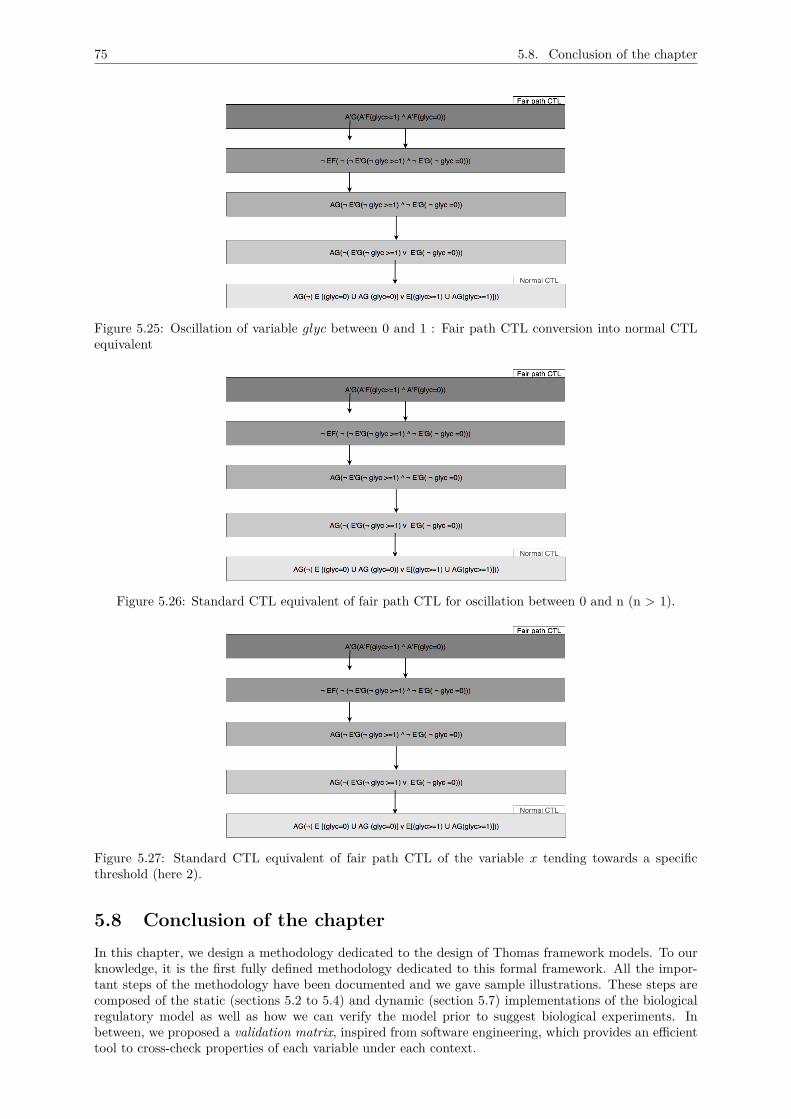
75 5.8. Conclusion of the chapter
Figure 5.25: Oscillation of variable glyc between 0 and 1 : Fair path CTL conversion into normal CTLequivalent
Figure 5.26: Standard CTL equivalent of fair path CTL for oscillation between 0 and n (n > 1).
Figure 5.27: Standard CTL equivalent of fair path CTL of the variable x tending towards a specificthreshold (here 2).
5.8 Conclusion of the chapterIn this chapter, we design a methodology dedicated to the design of Thomas framework models. To ourknowledge, it is the first fully defined methodology dedicated to this formal framework. All the impor-tant steps of the methodology have been documented and we gave sample illustrations. These steps arecomposed of the static (sections 5.2 to 5.4) and dynamic (section 5.7) implementations of the biologicalregulatory model as well as how we can verify the model prior to suggest biological experiments. Inbetween, we proposed a validation matrix, inspired from software engineering, which provides an efficienttool to cross-check properties of each variable under each context.

76 5.8. Conclusion of the chapter
We have shown how simulations can be useful to verify some initial well-known properties of a givensystem. The in-built non-deterministic aspect of the simulations motivates to validating certain proper-ties using CTL and the variant fair path CTL (detail is available in the Annex). This validation techniquehas been instrumental in the elaboration of all biologically sensible trajectories (irrespective of spuriousoscillations). In the next chapter, we will describe how we implemented all these functionalities in ourtool called DyMBioNet which allows to perform simulations as well as fair path CTL verifications.
CHAPTER 6DYMBIONET
6.1 IntroductionSmall biological networks can be designed and verified on paper and blackboard but this method is notfeasible for large networks. When the number of variables is significant, we are confronted with a hugenumber of possible state transition graphs and checking certain network properties can be complicatedand time consuming. More often, the extra but crucial step in modelling approach is casting the modelinto a formal, computable form that can be analysed rigorously using simulation and other mathematicalmethods 3.2. Furthermore, multiple simulations are needed to cater for main possible observable prop-erties or to refute a model, and this is where a software platform proves to be valuable.
On top of this, visually representing the network and being able to observe the dynamic evolutionsof the network is an important step to initiate discussions with the biologists. The advantages of simu-lations are therefore many folds: the network can be graphically represented, simulation of any size canbe done repeatedly, we can observe known properties as well as emerging properties, we can get usedto the network and attain faster diagnostics. We can also be exposed to counterexamples obtained bysimulation or model checking verification results. With the help of a simulator, the user can replay theviolating scenario to obtain useful debugging information. The model (or the dynamic property) canthen be adapted accordingly.
In the first section of this chapter, we will have a brief overview of four software that have been de-veloped for modelling complex networks using formal methods. We then give reasons why we have notuse them in our context. In later sections of this chapter, we will dive into the core functionalities ofDyMBioNet and show how it can be used to construct, analyse and simulate a biological network. Wecontinue to elaborate on how CTL can be helpful to establish important general biological propertiesinside DyMBioNet.
6.2 Existing software tools for the Thomas frameworkSome qualitative modelling tools already exist for the modelling of complex biological networks [122]. Wemention in this section, the advantages and drawbacks of four main tools namely: GINSim, GNA andSMBioNet, which are based on discrete formalisms.
6.2.1 GINsimGINsim (Gene Interaction Network simulation) is a computer tool for the modelling and simulation ofgenetic regulatory networks. GINsim allows the user to specify a model of a genetic regulatory networkin term of asynchronous, multivalued logical functions, and to simulate and/or analyse its qualitativedynamical behavior [131] as shown in Figure 6.1. This tool is platform–independent (Linux, Mac OS10.3+, Windows).GINsim is based on a compilation of Thomas networks with known parameter values into standard Petrinets. Consequently, it takes benefit of the whole corpus of analysis tools for Petri nets. The remarkableresult, proved by Chaouiya in [157], is that no inhibitory arcs are needed to perform the translation, sothat all decidability results are preserved. This provides a good theoretical ground and at the same timeaccounts for the popularity of GINsim. While this method is powerful, the complexity incurred by thistransformation into Petri nets is a major drawback. Moreover, it is somewhat paradoxical to translateThomas networks, where there is no concurrency on resources, into Petri nets. The complexity of the
77
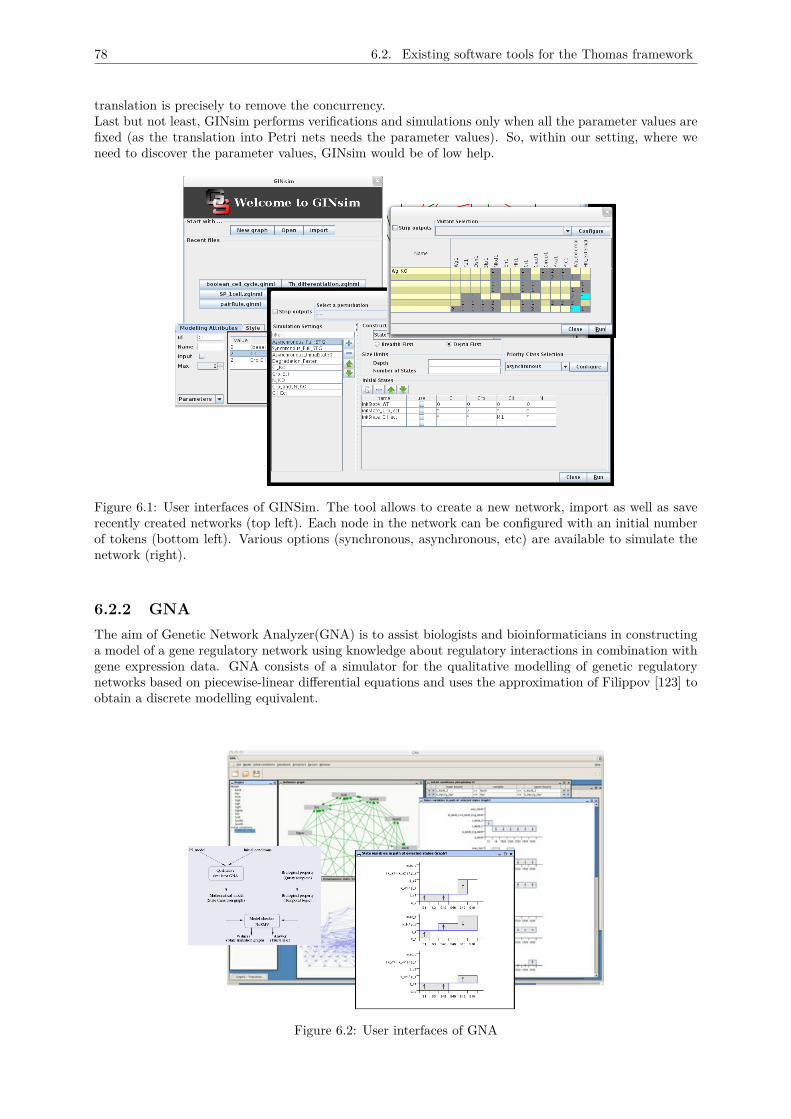
78 6.2. Existing software tools for the Thomas framework
translation is precisely to remove the concurrency.Last but not least, GINsim performs verifications and simulations only when all the parameter values arefixed (as the translation into Petri nets needs the parameter values). So, within our setting, where weneed to discover the parameter values, GINsim would be of low help.
Figure 6.1: User interfaces of GINSim. The tool allows to create a new network, import as well as saverecently created networks (top left). Each node in the network can be configured with an initial numberof tokens (bottom left). Various options (synchronous, asynchronous, etc) are available to simulate thenetwork (right).
6.2.2 GNAThe aim of Genetic Network Analyzer(GNA) is to assist biologists and bioinformaticians in constructinga model of a gene regulatory network using knowledge about regulatory interactions in combination withgene expression data. GNA consists of a simulator for the qualitative modelling of genetic regulatorynetworks based on piecewise-linear differential equations and uses the approximation of Filippov [123] toobtain a discrete modelling equivalent.
Figure 6.2: User interfaces of GNA
79 6.3. Description of the sample model
Figure 6.3: Singular states in GNA
Despite using a qualitative modelling approach, the methodology used by GNA is not the same as weadopted in this thesis. Our discrete formalism is based more on the logical aspects of nodes in the graph.We rely heavily on the discovery of values for kinetic parameters for system dynamics which we cannotsee in GNA. The implementation of CTL is somewhat comparable to our proposed software, where bothuse symbolic checker NuSMV, for validating CTL formulas. Figure 6.2 shows sample user interfaces ofthe GNA tool with several useful features, to list some: the model can be constructed from scratch andthe tool provides the possibility to import / export existing models; the ability to visualise the regulatorynetworks with an indication of all steady states; and finally, the specification of the dynamics in temporallogic.
Instead of using discrete values for its kinetic parameters, the user of GNA specifies inequality constraints[128]. The use of inequalities for thresholds and the application of differential equation for dynamic mod-elling of the network make GNA different from our approach which uses a logical implementation withdiscrete variables. For this reason, we prefer to extend our own platform to cater for these differences.
6.2.3 SMBioNet and TotemBioNetSMBioNet which stands for Symbolic Model checking of Biological Network is a command line tool cre-ated by Adrien Richard in 2007 [129]. It is mainly used for the modelling of gene regulatory networksbased on an extension of R.Thomas’ approach that integrate multiplexes. It acts as an interface betweenthe model and the associated model checking tool, NuSMV. Recently, several extensions of SMBioNethave been developed namely: HHLforBioNet and HyMBioNet [127]. In terms of functionality, it ressem-bles GNA with two differences: temporal model checking in the form of CTL is implemented in SMBioNetand we do not have singular states in SMBioNet. Nevertheless, the disadvantages of SMBioNet is the lackof visual simulation capability and it does not take into consideration fair CTL paths, which in returncould give rise to erroneous interpretation of the evaluation results. Since SMBioNet is an integral partof DyMBioNet, it is further discussed in section 6.5.2.
TotemBioNet is the successor of SMBioNet. Its aim is to combine Hoare Logic and CTL in order toimprove the efficacy of the enumeration phase that permit to automatically output all the correct pa-rameter valuations. As we will not use Hoare logic for our model of metabolism regulation, we have onlyintegrated SMBioNet into our DymBioNet software.
6.3 Description of the sample modelIn this section, we describe the sample network we will be using throughout this chapter as reference toshow some of the functionalities of DyMBioNet and at the same time demonstrate our methodologicalapproach (we called it model x-y throughout this text).
6.3.1 Main variablesWe use a simple network with 2 main variables: x and y. We assume they represent two biological entitieswhereby x is an activator of y and at the same time it is self-activator, and y is an inhibitor of x. Wealso put a control variable, c, which is an activator of x and is boolean.
6.3.2 Thresholdsx activates y at a threshold of 1, there is an auto-activation of x at threshold of 2 whereas y inhibitsx at a threshold of 1. As a reminder, whenever there is a unit threshold, it may be represented with
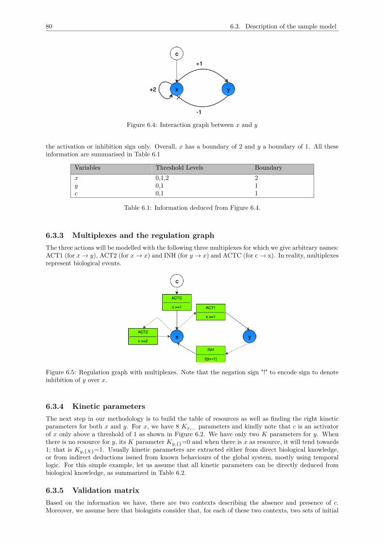
80 6.3. Description of the sample model
Figure 6.4: Interaction graph between x and y
the activation or inhibition sign only. Overall, x has a boundary of 2 and y a boundary of 1. All theseinformation are summarised in Table 6.1
Variables Threshold Levels Boundaryx 0,1,2 2y 0,1 1c 0,1 1
Table 6.1: Information deduced from Figure 6.4.
6.3.3 Multiplexes and the regulation graphThe three actions will be modelled with the following three multiplexes for which we give arbitrary names:ACT1 (for x→ y), ACT2 (for x→ x) and INH (for y → x) and ACTC (for c → x). In reality, multiplexesrepresent biological events.
Figure 6.5: Regulation graph with multiplexes. Note that the negation sign "!" to encode sign to denoteinhibition of y over x.
6.3.4 Kinetic parametersThe next step in our methodology is to build the table of resources as well as finding the right kineticparameters for both x and y. For x, we have 8 Kx,... parameters and kindly note that c is an activatorof x only above a threshold of 1 as shown in Figure 6.2. We have only two K parameters for y. Whenthere is no resource for y, its K parameter Ky,{}=0 and when there is x as resource, it will tend towards1; that is Ky,{X}=1. Usually kinetic parameters are extracted either from direct biological knowledge,or from indirect deductions issued from known behaviours of the global system, mostly using temporallogic. For this simple example, let us assume that all kinetic parameters can be directly deduced frombiological knowledge, as summarized in Table 6.2.
6.3.5 Validation matrixBased on the information we have, there are two contexts describing the absence and presence of c.Moreover, we assume here that biologists consider that, for each of these two contexts, two sets of initial
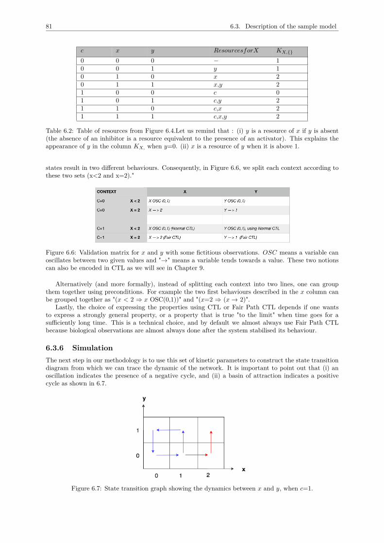
81 6.3. Description of the sample model
c x y ResourcesforX KX,{}
0 0 0 − 10 0 1 y 10 1 0 x 20 1 1 x,y 21 0 0 c 01 0 1 c,y 21 1 0 c,x 21 1 1 c,x,y 2
Table 6.2: Table of resources from Figure 6.4.Let us remind that : (i) y is a resource of x if y is absent(the absence of an inhibitor is a resource equivalent to the presence of an activator). This explains theappearance of y in the column KX, when y=0. (ii) x is a resource of y when it is above 1.
states result in two different behaviours. Consequently, in Figure 6.6, we split each context according tothese two sets (x<2 and x=2)."
Figure 6.6: Validation matrix for x and y with some fictitious observations. OSC means a variable canoscillates between two given values and "→" means a variable tends towards a value. These two notionscan also be encoded in CTL as we will see in Chapter 9.
Alternatively (and more formally), instead of splitting each context into two lines, one can groupthem together using preconditions. For example the two first behaviours described in the x column canbe grouped together as "(x < 2 ⇒ x OSC(0,1))" and "(x=2 ⇒ (x→ 2)".
Lastly, the choice of expressing the properties using CTL or Fair Path CTL depends if one wantsto express a strongly general property, or a property that is true "to the limit" when time goes for asufficiently long time. This is a technical choice, and by default we almost always use Fair Path CTLbecause biological observations are almost always done after the system stabilised its behaviour.
6.3.6 SimulationThe next step in our methodology is to use this set of kinetic parameters to construct the state transitiondiagram from which we can trace the dynamic of the network. It is important to point out that (i) anoscillation indicates the presence of a negative cycle, and (ii) a basin of attraction indicates a positivecycle as shown in 6.7.
Figure 6.7: State transition graph showing the dynamics between x and y, when c=1.
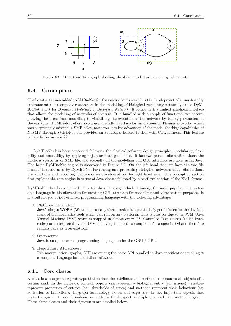
82 6.4. Conception
Figure 6.8: State transition graph showing the dynamics between x and y, when c=0.
6.4 ConceptionThe latest extension added to SMBioNet for the needs of our research is the development of a user-friendlyenvironment to accompany researchers in the modelling of biological regulatory networks, called DyM-BioNet, short for Dynamic Modelling of Biological Network. It comes with a unified graphical interfacethat allows the modelling of networks of any size. It is bundled with a couple of functionalities accom-panying the users from modelling to visualising the evolution of the network by tuning parameters ofthe variables. DyMBioNet offers also a user-friendly interface for simulations of Thomas networks, whichwas surprisingly missing in SMBioNet, moreover it takes advantage of the model checking capabilities ofNuSMV through SMBioNet but provides an additional feature to deal with CTL fairness. This featureis detailed in section ??.
DyMBioNet has been conceived following the classical software design principles: modularity, flexi-bility and reusability, by applying object-oriented guidelines. It has two parts: information about themodel is stored in an XML file, and secondly all the modelling and GUI interfaces are done using Java.The basic DyMBioNet engine is showcased in Figure 6.9. On the left hand side, we have the two fileformats that are used by DyMBioNet for storing and processing biological networks data. Simulations,visualisations and reporting functionalities are showed on the right hand side. This conception sectionfirst explains the core engine in terms of Java classes followed by a brief explanation of the XML format.
DyMBioNet has been created using the Java language which is among the most popular and prefer-able language in bioinformatics for creating GUI interfaces for modelling and visualisation purposes. Itis a full fledged object-oriented programming language with the following advantages:
1. Platform-independentJava’s slogan WORA (Write one, run anywhere) makes it a particularly good choice for the develop-ment of bioinformatics tools which can run on any platform. This is possible due to its JVM (JavaVirtual Machine JVM) which is shipped in almost every OS. Compiled Java classes (called byte-codes) are interpreted by the JVM removing the need to compile it for a specific OS and thereforerenders Java as cross-platform.
2. Open-sourceJava is an open-source programming language under the GNU / GPL.
3. Huge library API supportFile manipulation, graphs, GUI are among the basic API bundled in Java specifications making ita complete language for simulation software.
6.4.1 Core classesA class is a blueprint or prototype that defines the attributes and methods common to all objects of acertain kind. In the biological context, objects can represent a biological entity (eg. a gene), variablesrepresent properties of entities (eg. thresholds of genes) and methods represent their behaviour (eg.activation or inhibition). In graph terminology, nodes and edges are the two important aspects thatmake the graph. In our formalism, we added a third aspect, multiplex, to make the metabolic graph.These three classes and their signatures are detailed below.
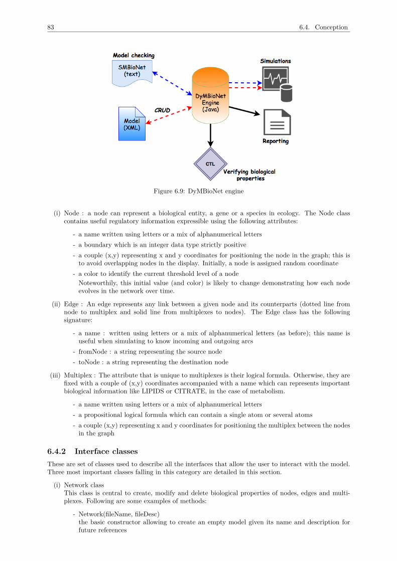
83 6.4. Conception
Figure 6.9: DyMBioNet engine
(i) Node : a node can represent a biological entity, a gene or a species in ecology. The Node classcontains useful regulatory information expressible using the following attributes:
- a name written using letters or a mix of alphanumerical letters- a boundary which is an integer data type strictly positive- a couple (x,y) representing x and y coordinates for positioning the node in the graph; this isto avoid overlapping nodes in the display. Initially, a node is assigned random coordinate
- a color to identify the current threshold level of a nodeNoteworthily, this initial value (and color) is likely to change demonstrating how each nodeevolves in the network over time.
(ii) Edge : An edge represents any link between a given node and its counterparts (dotted line fromnode to multiplex and solid line from multiplexes to nodes). The Edge class has the followingsignature:
- a name : written using letters or a mix of alphanumerical letters (as before); this name isuseful when simulating to know incoming and outgoing arcs
- fromNode : a string representing the source node- toNode : a string representing the destination node
(iii) Multiplex : The attribute that is unique to multiplexes is their logical formula. Otherwise, they arefixed with a couple of (x,y) coordinates accompanied with a name which can represents importantbiological information like LIPIDS or CITRATE, in the case of metabolism.
- a name written using letters or a mix of alphanumerical letters- a propositional logical formula which can contain a single atom or several atoms- a couple (x,y) representing x and y coordinates for positioning the multiplex between the nodesin the graph
6.4.2 Interface classesThese are set of classes used to describe all the interfaces that allow the user to interact with the model.Three most important classes falling in this category are detailed in this section.
(i) Network classThis class is central to create, modify and delete biological properties of nodes, edges and multi-plexes. Following are some examples of methods:
- Network(fileName, fileDesc)the basic constructor allowing to create an empty model given its name and description forfuture references
84 6.4. Conception
- addX(attributes)where X represents a Node, an Edge or a Multiplex; the same naming is used for delete andupdate
- addParameter(..) and updateKParameter(..) are the set of methods for creating and deletingK parameters for each variable
(ii) DyMBioNet classThis is the main entry point to the software when the application is launched. It represents thedashboard of the software.
- createGraph(..)This method will create the graph with the set of nodes, edges and multiplexes by retrievingdata stored in the XML file.
- showGraph(...)This method will display the graph on the interface.
- explore(...)This method is used to simulate the network with initial parameters provided by the user.
(iii) KineticScreen classKinetic parameterisation is done in this class and is divided in two parts. One with an outline ofthe set of resources for the variable under investigation in a tabular form. The second shows thevariable graphically which allows the user to reason locally with all its incoming and outgoing arcs.
- KineticScreen(..)Default constructor to show the interface for displaying the list of K parameters which can beupdated directly.
- generateKineticGraph(..)Display the set of resources of a particular node to facilitate the user with the task of identifyingthe K parameters.
- isActivator(..)This boolean method is to verify the formula of a given multiplex to check if it an activatoror inhibitor.
The complete code for the above-mentioned classes are found in Annex11.8 together with other javaclasses in the package fr.unice.
6.4.3 Model formatMany possibilities exist to store biological models and their related information of interest; for exampleusing text files, a local database, or the widely used XML format. Text files contain delimiters andinformation stored are unstructured making it difficult to be interpreted and managed. The use of alocal database is highly dependent on a web server for interfacing with the software. Updating networkinformation is cumbersome and the migration of the networks would require backing database tables whichis not too practical. Notably, XML becomes a good choice as a modelling format and its practicalityis outlined hereafter. This short section is by no means a complete guide to XML or any if its validityformat, but instead is intended as a broad overview of how it is used to represent the information ofvariables and their interactions in the biological network.
XML, which stands for eXtensible Markup Language, has been here since more than a decade fromnow. In our context, its usefulness is justified as follows:
• Simplicity - Information coded in XML is easy to read and understand, plus it is understood byalmost all programming languages (through API)
• Openness - XML is a W3C standard, endorsed by software industry market leaders.
• Extensibility - There is no fixed set of tags. New tags can be created as and when needed. Thisis particular interesting in our case: for example a <node> element for representing a variable, a<mult> tag linking it to a multiplex, etc.
• Self-description - Each tag or attribute speaks clearly about its meaning in the file. For example a<nodes> tag refers to the list of nodes in the graph whereas a <node> tag refers to a particularnode with some fixed attributes.
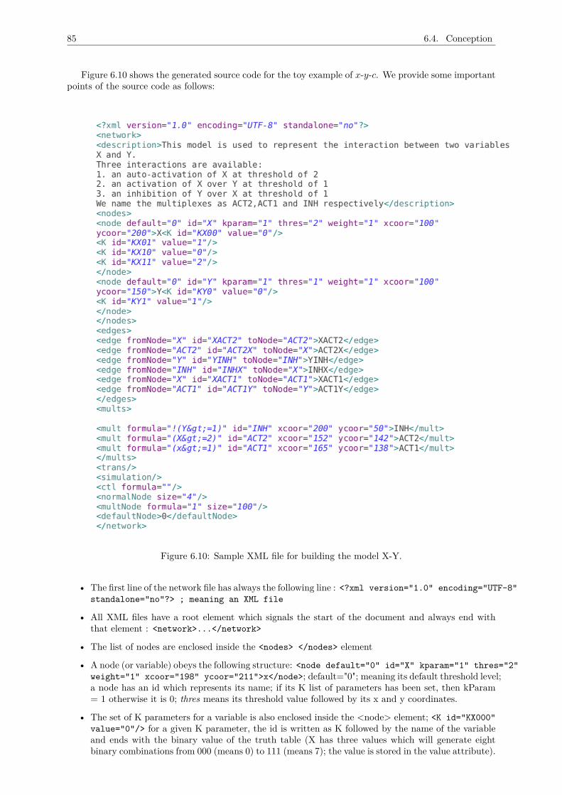
85 6.4. Conception
Figure 6.10 shows the generated source code for the toy example of x-y-c. We provide some importantpoints of the source code as follows:
Figure 6.10: Sample XML file for building the model X-Y.
• The first line of the network file has always the following line : <?xml version="1.0" encoding="UTF-8"standalone="no"?> ; meaning an XML file
• All XML files have a root element which signals the start of the document and always end withthat element : <network>...</network>
• The list of nodes are enclosed inside the <nodes> </nodes> element
• A node (or variable) obeys the following structure: <node default="0" id="X" kparam="1" thres="2"weight="1" xcoor="198" ycoor="211">x</node>; default="0"; meaning its default threshold level;a node has an id which represents its name; if its K list of parameters has been set, then kParam= 1 otherwise it is 0; thres means its threshold value followed by its x and y coordinates.
• The set of K parameters for a variable is also enclosed inside the <node> element; <K id="KX000"value="0"/> for a given K parameter, the id is written as K followed by the name of the variableand ends with the binary value of the truth table (X has three values which will generate eightbinary combinations from 000 (means 0) to 111 (means 7); the value is stored in the value attribute).
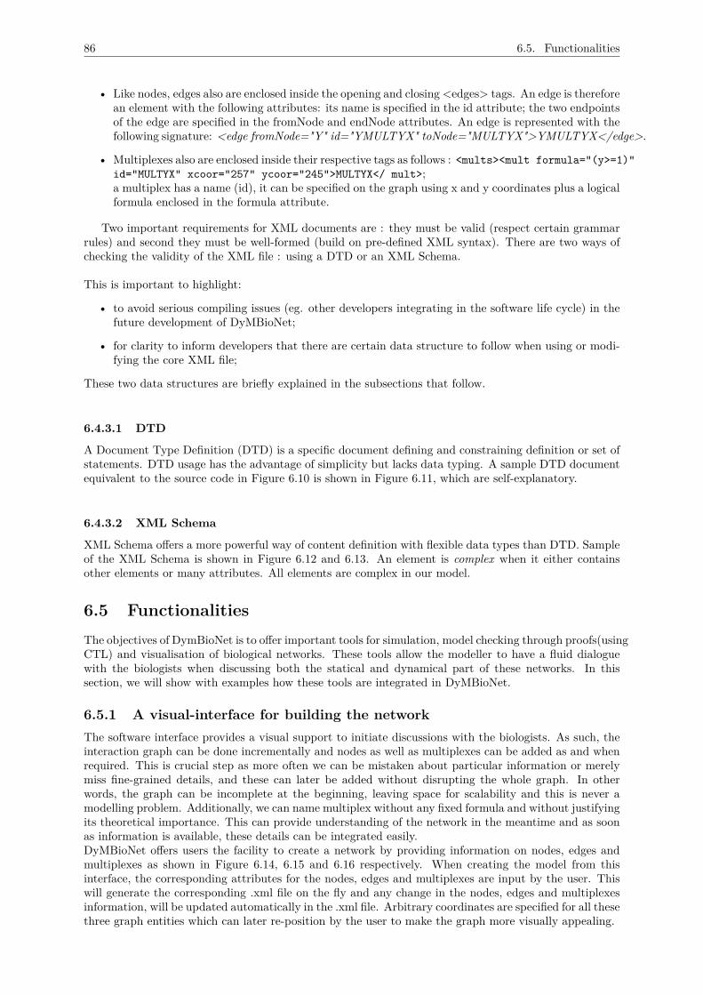
86 6.5. Functionalities
• Like nodes, edges also are enclosed inside the opening and closing <edges> tags. An edge is thereforean element with the following attributes: its name is specified in the id attribute; the two endpointsof the edge are specified in the fromNode and endNode attributes. An edge is represented with thefollowing signature: <edge fromNode="Y" id="YMULTYX" toNode="MULTYX">YMULTYX</edge>.
• Multiplexes also are enclosed inside their respective tags as follows : <mults><mult formula="(y>=1)"id="MULTYX" xcoor="257" ycoor="245">MULTYX</ mult>;a multiplex has a name (id), it can be specified on the graph using x and y coordinates plus a logicalformula enclosed in the formula attribute.
Two important requirements for XML documents are : they must be valid (respect certain grammarrules) and second they must be well-formed (build on pre-defined XML syntax). There are two ways ofchecking the validity of the XML file : using a DTD or an XML Schema.
This is important to highlight:
• to avoid serious compiling issues (eg. other developers integrating in the software life cycle) in thefuture development of DyMBioNet;
• for clarity to inform developers that there are certain data structure to follow when using or modi-fying the core XML file;
These two data structures are briefly explained in the subsections that follow.
6.4.3.1 DTD
A Document Type Definition (DTD) is a specific document defining and constraining definition or set ofstatements. DTD usage has the advantage of simplicity but lacks data typing. A sample DTD documentequivalent to the source code in Figure 6.10 is shown in Figure 6.11, which are self-explanatory.
6.4.3.2 XML Schema
XML Schema offers a more powerful way of content definition with flexible data types than DTD. Sampleof the XML Schema is shown in Figure 6.12 and 6.13. An element is complex when it either containsother elements or many attributes. All elements are complex in our model.
6.5 FunctionalitiesThe objectives of DymBioNet is to offer important tools for simulation, model checking through proofs(usingCTL) and visualisation of biological networks. These tools allow the modeller to have a fluid dialoguewith the biologists when discussing both the statical and dynamical part of these networks. In thissection, we will show with examples how these tools are integrated in DyMBioNet.
6.5.1 A visual-interface for building the networkThe software interface provides a visual support to initiate discussions with the biologists. As such, theinteraction graph can be done incrementally and nodes as well as multiplexes can be added as and whenrequired. This is crucial step as more often we can be mistaken about particular information or merelymiss fine-grained details, and these can later be added without disrupting the whole graph. In otherwords, the graph can be incomplete at the beginning, leaving space for scalability and this is never amodelling problem. Additionally, we can name multiplex without any fixed formula and without justifyingits theoretical importance. This can provide understanding of the network in the meantime and as soonas information is available, these details can be integrated easily.DyMBioNet offers users the facility to create a network by providing information on nodes, edges andmultiplexes as shown in Figure 6.14, 6.15 and 6.16 respectively. When creating the model from thisinterface, the corresponding attributes for the nodes, edges and multiplexes are input by the user. Thiswill generate the corresponding .xml file on the fly and any change in the nodes, edges and multiplexesinformation, will be updated automatically in the .xml file. Arbitrary coordinates are specified for all thesethree graph entities which can later re-position by the user to make the graph more visually appealing.
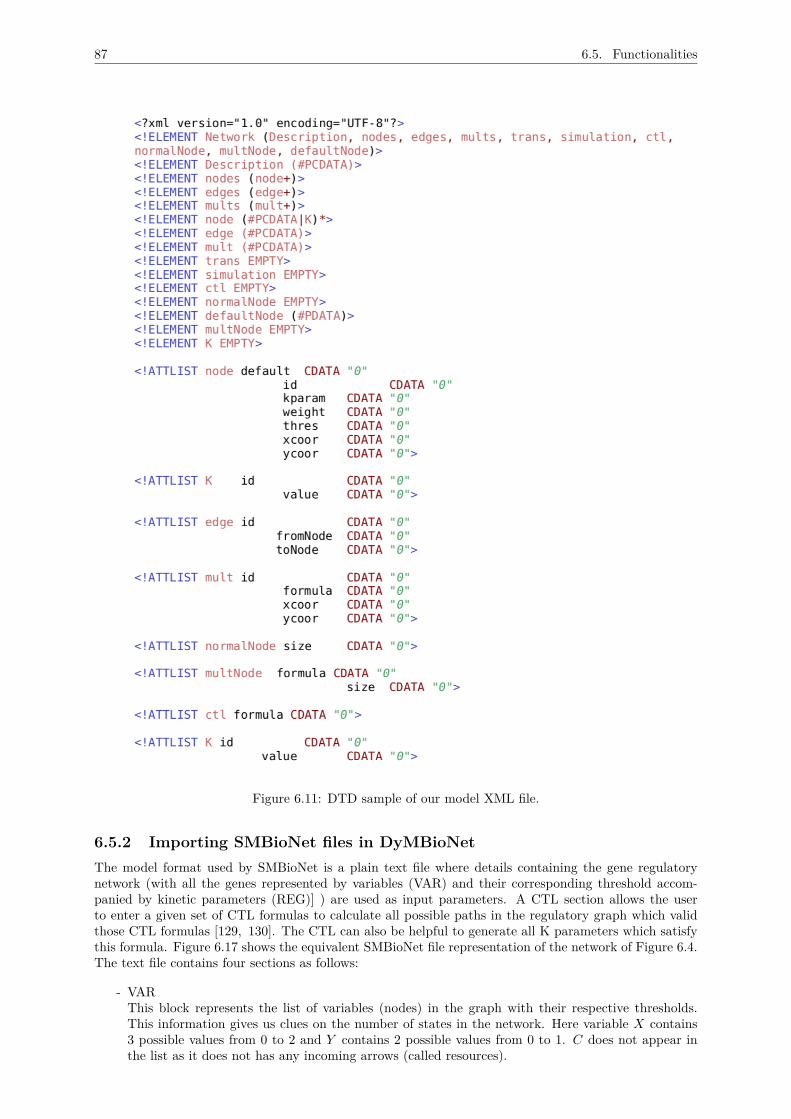
87 6.5. Functionalities
Figure 6.11: DTD sample of our model XML file.
6.5.2 Importing SMBioNet files in DyMBioNetThe model format used by SMBioNet is a plain text file where details containing the gene regulatorynetwork (with all the genes represented by variables (VAR) and their corresponding threshold accom-panied by kinetic parameters (REG)] ) are used as input parameters. A CTL section allows the userto enter a given set of CTL formulas to calculate all possible paths in the regulatory graph which validthose CTL formulas [129, 130]. The CTL can also be helpful to generate all K parameters which satisfythis formula. Figure 6.17 shows the equivalent SMBioNet file representation of the network of Figure 6.4.The text file contains four sections as follows:
- VARThis block represents the list of variables (nodes) in the graph with their respective thresholds.This information gives us clues on the number of states in the network. Here variable X contains3 possible values from 0 to 2 and Y contains 2 possible values from 0 to 1. C does not appear inthe list as it does not has any incoming arrows (called resources).
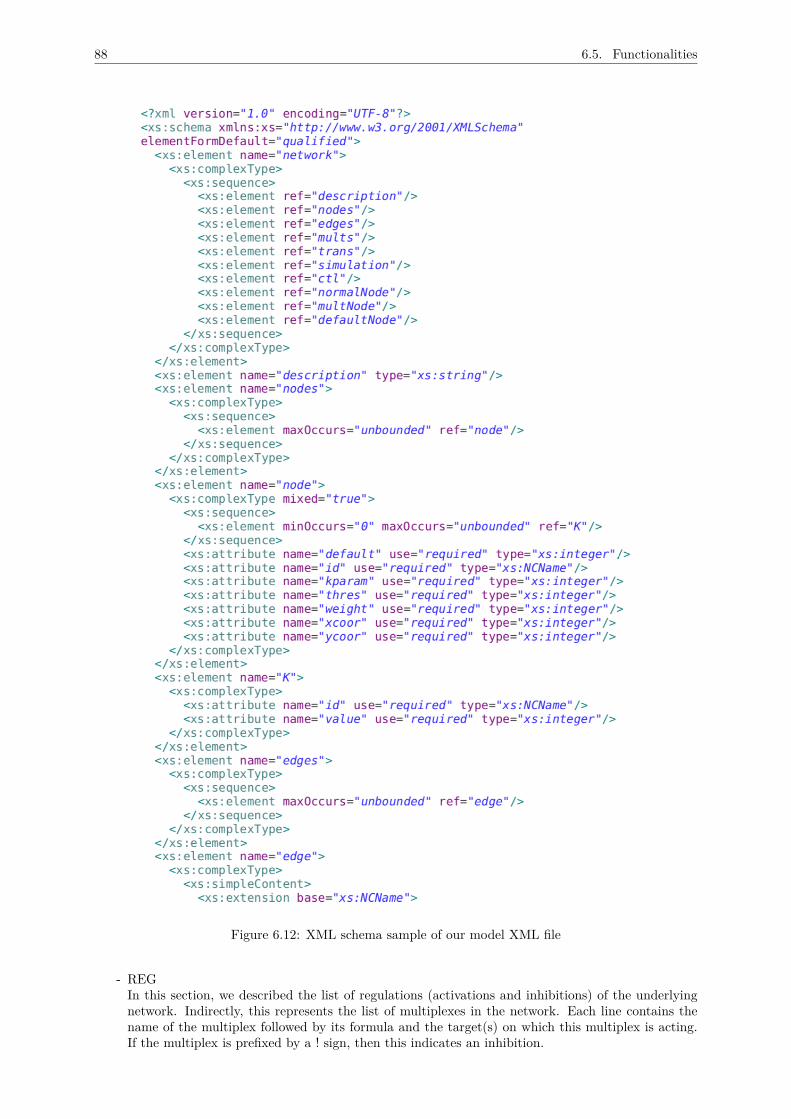
88 6.5. Functionalities
Figure 6.12: XML schema sample of our model XML file
- REGIn this section, we described the list of regulations (activations and inhibitions) of the underlyingnetwork. Indirectly, this represents the list of multiplexes in the network. Each line contains thename of the multiplex followed by its formula and the target(s) on which this multiplex is acting.If the multiplex is prefixed by a ! sign, then this indicates an inhibition.
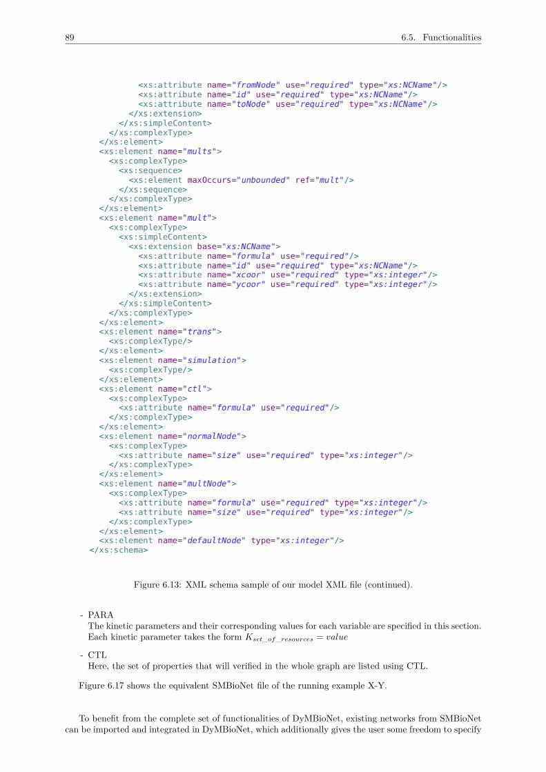
89 6.5. Functionalities
Figure 6.13: XML schema sample of our model XML file (continued).
- PARAThe kinetic parameters and their corresponding values for each variable are specified in this section.Each kinetic parameter takes the form Kset_of_resources = value
- CTLHere, the set of properties that will verified in the whole graph are listed using CTL.
Figure 6.17 shows the equivalent SMBioNet file of the running example X-Y.
To benefit from the complete set of functionalities of DyMBioNet, existing networks from SMBioNetcan be imported and integrated in DyMBioNet, which additionally gives the user some freedom to specify
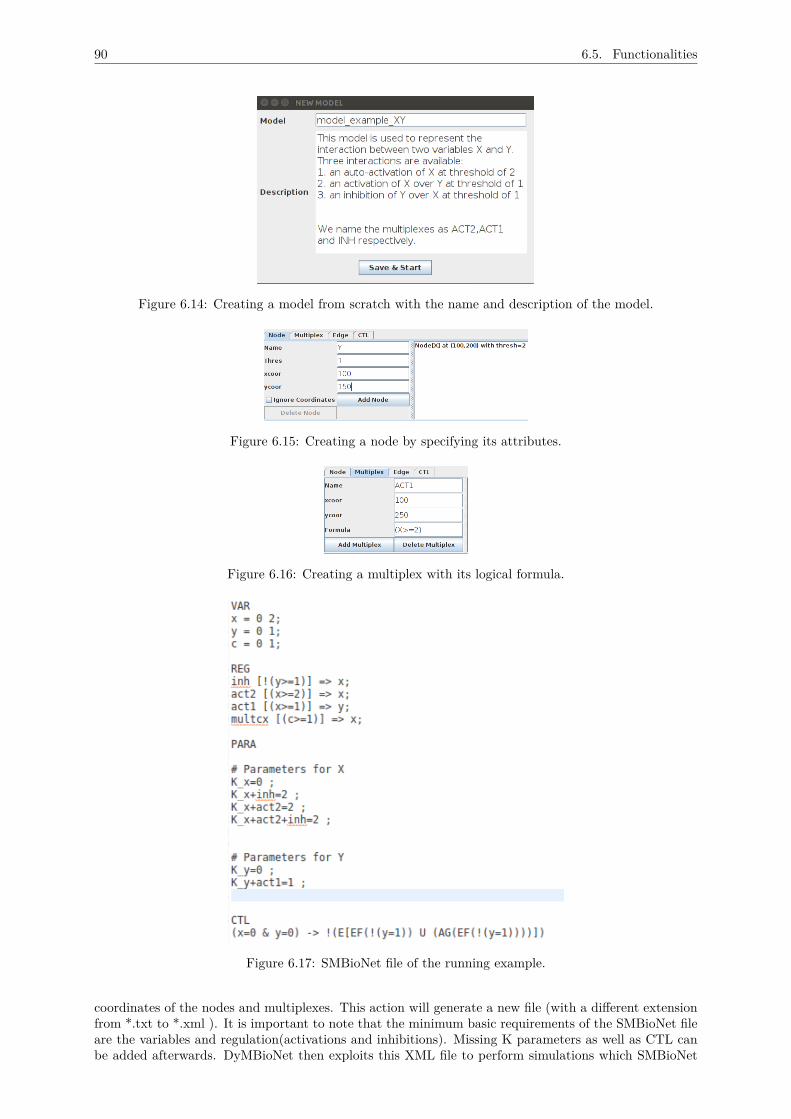
90 6.5. Functionalities
Figure 6.14: Creating a model from scratch with the name and description of the model.
Figure 6.15: Creating a node by specifying its attributes.
Figure 6.16: Creating a multiplex with its logical formula.
Figure 6.17: SMBioNet file of the running example.
coordinates of the nodes and multiplexes. This action will generate a new file (with a different extensionfrom *.txt to *.xml ). It is important to note that the minimum basic requirements of the SMBioNet fileare the variables and regulation(activations and inhibitions). Missing K parameters as well as CTL canbe added afterwards. DyMBioNet then exploits this XML file to perform simulations which SMBioNet
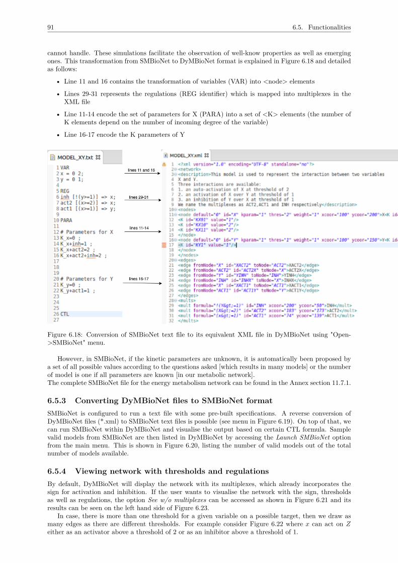
91 6.5. Functionalities
cannot handle. These simulations facilitate the observation of well-know properties as well as emergingones. This transformation from SMBioNet to DyMBioNet format is explained in Figure 6.18 and detailedas follows:
• Line 11 and 16 contains the transformation of variables (VAR) into <node> elements
• Lines 29-31 represents the regulations (REG identifier) which is mapped into multiplexes in theXML file
• Line 11-14 encode the set of parameters for X (PARA) into a set of <K> elements (the number ofK elements depend on the number of incoming degree of the variable)
• Line 16-17 encode the K parameters of Y
Figure 6.18: Conversion of SMBioNet text file to its equivalent XML file in DyMBioNet using "Open->SMBioNet" menu.
However, in SMBioNet, if the kinetic parameters are unknown, it is automatically been proposed bya set of all possible values according to the questions asked [which results in many models] or the numberof model is one if all parameters are known [in our metabolic network].The complete SMBioNet file for the energy metabolism network can be found in the Annex section 11.7.1.
6.5.3 Converting DyMBioNet files to SMBioNet formatSMBioNet is configured to run a text file with some pre-built specifications. A reverse conversion ofDyMBioNet files (*.xml) to SMBioNet text files is possible (see menu in Figure 6.19). On top of that, wecan run SMBioNet within DyMBioNet and visualise the output based on certain CTL formula. Samplevalid models from SMBioNet are then listed in DyMBioNet by accessing the Launch SMBioNet optionfrom the main menu. This is shown in Figure 6.20, listing the number of valid models out of the totalnumber of models available.
6.5.4 Viewing network with thresholds and regulationsBy default, DyMBioNet will display the network with its multiplexes, which already incorporates thesign for activation and inhibition. If the user wants to visualise the network with the sign, thresholdsas well as regulations, the option See w/o multiplexes can be accessed as shown in Figure 6.21 and itsresults can be seen on the left hand side of Figure 6.23.
In case, there is more than one threshold for a given variable on a possible target, then we draw asmany edges as there are different thresholds. For example consider Figure 6.22 where x can act on Zeither as an activator above a threshold of 2 or as an inhibitor above a threshold of 1.
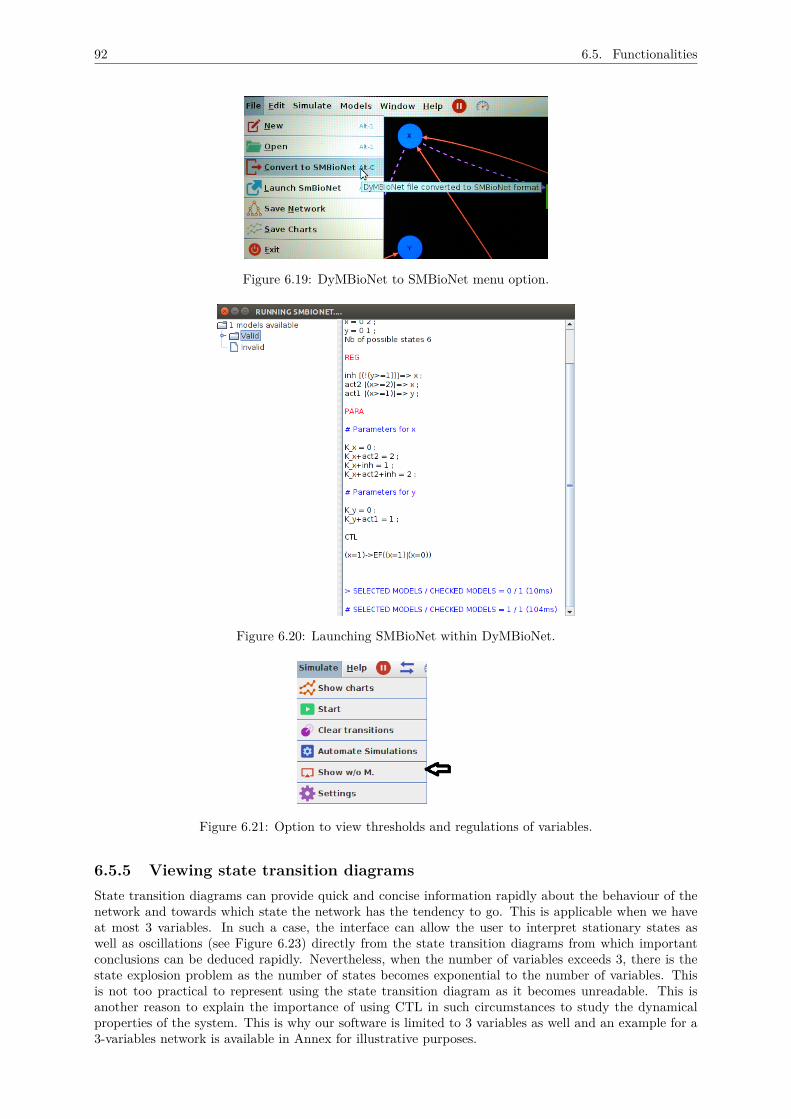
92 6.5. Functionalities
Figure 6.19: DyMBioNet to SMBioNet menu option.
Figure 6.20: Launching SMBioNet within DyMBioNet.
Figure 6.21: Option to view thresholds and regulations of variables.
6.5.5 Viewing state transition diagramsState transition diagrams can provide quick and concise information rapidly about the behaviour of thenetwork and towards which state the network has the tendency to go. This is applicable when we haveat most 3 variables. In such a case, the interface can allow the user to interpret stationary states aswell as oscillations (see Figure 6.23) directly from the state transition diagrams from which importantconclusions can be deduced rapidly. Nevertheless, when the number of variables exceeds 3, there is thestate explosion problem as the number of states becomes exponential to the number of variables. Thisis not too practical to represent using the state transition diagram as it becomes unreadable. This isanother reason to explain the importance of using CTL in such circumstances to study the dynamicalproperties of the system. This is why our software is limited to 3 variables as well and an example for a3-variables network is available in Annex for illustrative purposes.
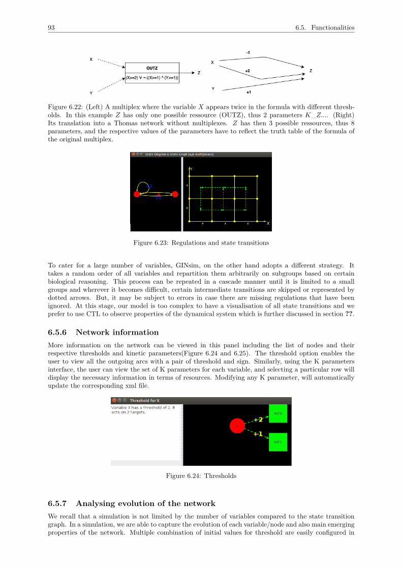
93 6.5. Functionalities
Figure 6.22: (Left) A multiplex where the variable X appears twice in the formula with different thresh-olds. In this example Z has only one possible ressource (OUTZ), thus 2 parameters K_Z.... (Right)Its translation into a Thomas network without multiplexes. Z has then 3 possible ressources, thus 8parameters, and the respective values of the parameters have to reflect the truth table of the formula ofthe original multiplex.
Figure 6.23: Regulations and state transitions
To cater for a large number of variables, GINsim, on the other hand adopts a different strategy. Ittakes a random order of all variables and repartition them arbitrarily on subgroups based on certainbiological reasoning. This process can be repeated in a cascade manner until it is limited to a smallgroups and wherever it becomes difficult, certain intermediate transitions are skipped or represented bydotted arrows. But, it may be subject to errors in case there are missing regulations that have beenignored. At this stage, our model is too complex to have a visualisation of all state transitions and weprefer to use CTL to observe properties of the dynamical system which is further discussed in section ??.
6.5.6 Network informationMore information on the network can be viewed in this panel including the list of nodes and theirrespective thresholds and kinetic parameters(Figure 6.24 and 6.25). The threshold option enables theuser to view all the outgoing arcs with a pair of threshold and sign. Similarly, using the K parametersinterface, the user can view the set of K parameters for each variable, and selecting a particular row willdisplay the necessary information in terms of resources. Modifying any K parameter, will automaticallyupdate the corresponding xml file.
Figure 6.24: Thresholds
6.5.7 Analysing evolution of the networkWe recall that a simulation is not limited by the number of variables compared to the state transitiongraph. In a simulation, we are able to capture the evolution of each variable/node and also main emergingproperties of the network. Multiple combination of initial values for threshold are easily configured in
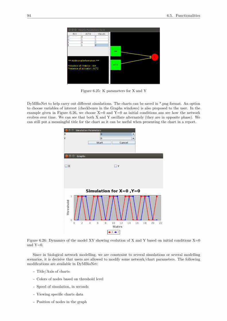
94 6.5. Functionalities
Figure 6.25: K parameters for X and Y
DyMBioNet to help carry out different simulations. The charts can be saved in *.png format. An optionto choose variables of interest (checkboxes in the Graphs windows) is also proposed to the user. In theexample given in Figure 6.26, we choose X=0 and Y=0 as initial conditions ans see how the networkevolves over time. We can see that both X and Y oscillate alternately (they are in opposite phase). Wecan still put a meaningful title for the chart as it can be useful when presenting the chart in a report.
Figure 6.26: Dynamics of the model XY showing evolution of X and Y based on initial conditions X=0and Y=0.
Since in biological network modelling, we are constraint to several simulations or several modellingscenarios, it is decisive that users are allowed to modify some network/chart parameters. The followingmodifications are available in DyMBioNet:
- Title/Axis of charts
- Colors of nodes based on threshold level
- Speed of simulation, in seconds
- Viewing specific charts data
- Position of nodes in the graph
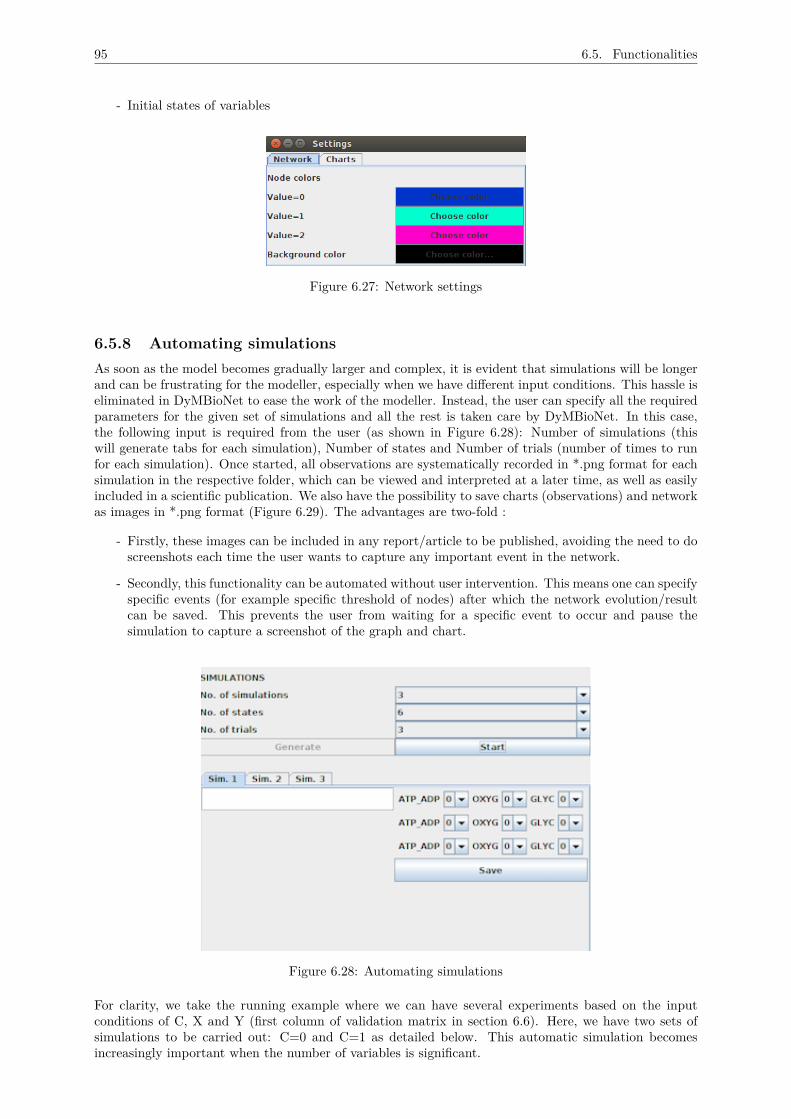
95 6.5. Functionalities
- Initial states of variables
Figure 6.27: Network settings
6.5.8 Automating simulationsAs soon as the model becomes gradually larger and complex, it is evident that simulations will be longerand can be frustrating for the modeller, especially when we have different input conditions. This hassle iseliminated in DyMBioNet to ease the work of the modeller. Instead, the user can specify all the requiredparameters for the given set of simulations and all the rest is taken care by DyMBioNet. In this case,the following input is required from the user (as shown in Figure 6.28): Number of simulations (thiswill generate tabs for each simulation), Number of states and Number of trials (number of times to runfor each simulation). Once started, all observations are systematically recorded in *.png format for eachsimulation in the respective folder, which can be viewed and interpreted at a later time, as well as easilyincluded in a scientific publication. We also have the possibility to save charts (observations) and networkas images in *.png format (Figure 6.29). The advantages are two-fold :
- Firstly, these images can be included in any report/article to be published, avoiding the need to doscreenshots each time the user wants to capture any important event in the network.
- Secondly, this functionality can be automated without user intervention. This means one can specifyspecific events (for example specific threshold of nodes) after which the network evolution/resultcan be saved. This prevents the user from waiting for a specific event to occur and pause thesimulation to capture a screenshot of the graph and chart.
Figure 6.28: Automating simulations
For clarity, we take the running example where we can have several experiments based on the inputconditions of C, X and Y (first column of validation matrix in section 6.6). Here, we have two sets ofsimulations to be carried out: C=0 and C=1 as detailed below. This automatic simulation becomesincreasingly important when the number of variables is significant.
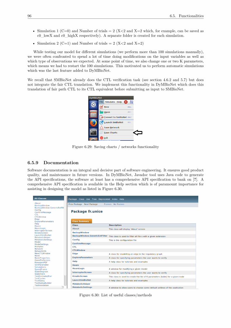
96 6.5. Functionalities
• Simulation 1 (C=0) and Number of trials = 2 (X<2 and X=2 which, for example, can be saved asc0_lowX and c0_highX respectively). A separate folder is created for each simulation.
• Simulation 2 (C=1) and Number of trials = 2 (X<2 and X=2)
While testing our model for different simulations (we perform more than 100 simulations manually),we were often confronted to spend a lot of time doing modifications on the input variables as well aswhich type of observations we expected. At some point of time, we also change one or two K parameters,which means we had to restart the 100 simulations. This motivated us to perform automatic simulationswhich was the last feature added to DyMBioNet.
We recall that SMBioNet already does the CTL verification task (see section 4.6.2 and 5.7) but doesnot integrate the fair CTL translation. We implement this functionality in DyMBioNet which does thistranslation of fair path CTL to its CTL equivalent before submitting as input to SMBioNet.
Figure 6.29: Saving charts / networks functionality
6.5.9 DocumentationSoftware documentation is an integral and decisive part of software engineering. It ensures good productquality, and maintenance in future versions. In DyMBioNet, Javadoc tool uses Java code to generatethe API specifications, the software at least has a comprehensive API specification to bank on [?]. Acomprehensive API specification is available in the Help section which is of paramount importance forassisting in designing the model as listed in Figure 6.30.
Figure 6.30: List of useful classes/methods
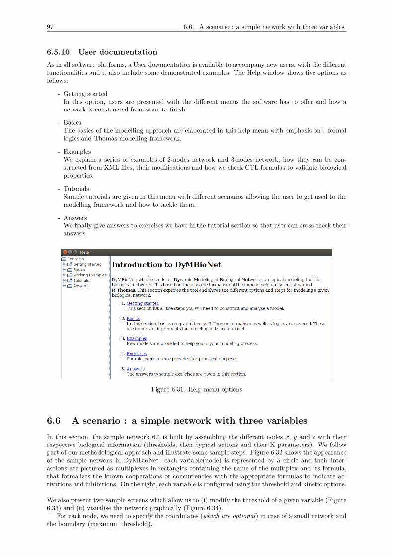
97 6.6. A scenario : a simple network with three variables
6.5.10 User documentationAs in all software platforms, a User documentation is available to accompany new users, with the differentfunctionalities and it also include some demonstrated examples. The Help window shows five options asfollows:
- Getting startedIn this option, users are presented with the different menus the software has to offer and how anetwork is constructed from start to finish.
- BasicsThe basics of the modelling approach are elaborated in this help menu with emphasis on : formallogics and Thomas modelling framework.
- ExamplesWe explain a series of examples of 2-nodes network and 3-nodes network, how they can be con-structed from XML files, their modifications and how we check CTL formulas to validate biologicalproperties.
- TutorialsSample tutorials are given in this menu with different scenarios allowing the user to get used to themodelling framework and how to tackle them.
- AnswersWe finally give answers to exercises we have in the tutorial section so that user can cross-check theiranswers.
Figure 6.31: Help menu options
6.6 A scenario : a simple network with three variablesIn this section, the sample network 6.4 is built by assembling the different nodes x, y and c with theirrespective biological information (thresholds, their typical actions and their K parameters). We followpart of our methodological approach and illustrate some sample steps. Figure 6.32 shows the appearanceof the sample network in DyMBioNet: each variable(node) is represented by a circle and their inter-actions are pictured as multiplexes in rectangles containing the name of the multiplex and its formula,that formalizes the known cooperations or concurrencies with the appropriate formulas to indicate ac-tivations and inhibitions. On the right, each variable is configured using the threshold and kinetic options.
We also present two sample screens which allow us to (i) modify the threshold of a given variable (Figure6.33) and (ii) visualise the network graphically (Figure 6.34).
For each node, we need to specify the coordinates (which are optional) in case of a small network andthe boundary (maximum threshold).
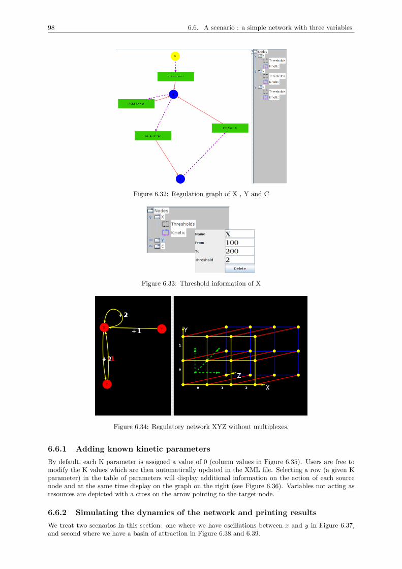
98 6.6. A scenario : a simple network with three variables
Figure 6.32: Regulation graph of X , Y and C
Figure 6.33: Threshold information of X
Figure 6.34: Regulatory network XYZ without multiplexes.
6.6.1 Adding known kinetic parametersBy default, each K parameter is assigned a value of 0 (column values in Figure 6.35). Users are free tomodify the K values which are then automatically updated in the XML file. Selecting a row (a given Kparameter) in the table of parameters will display additional information on the action of each sourcenode and at the same time display on the graph on the right (see Figure 6.36). Variables not acting asresources are depicted with a cross on the arrow pointing to the target node.
6.6.2 Simulating the dynamics of the network and printing resultsWe treat two scenarios in this section: one where we have oscillations between x and y in Figure 6.37,and second where we have a basin of attraction in Figure 6.38 and 6.39.
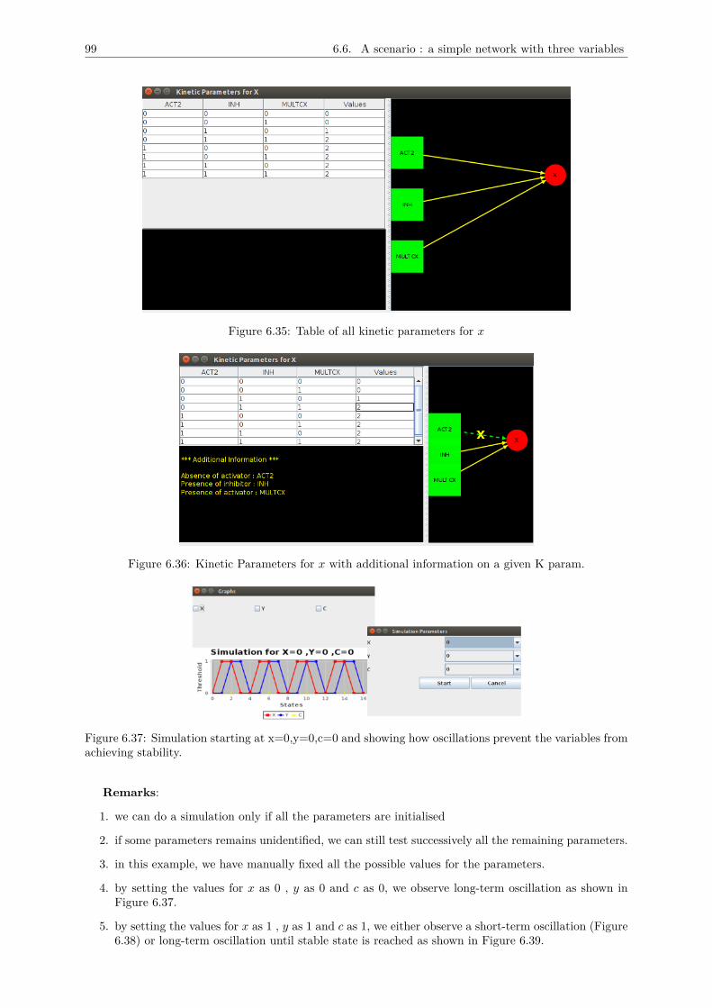
99 6.6. A scenario : a simple network with three variables
Figure 6.35: Table of all kinetic parameters for x
Figure 6.36: Kinetic Parameters for x with additional information on a given K param.
Figure 6.37: Simulation starting at x=0,y=0,c=0 and showing how oscillations prevent the variables fromachieving stability.
Remarks:
1. we can do a simulation only if all the parameters are initialised
2. if some parameters remains unidentified, we can still test successively all the remaining parameters.
3. in this example, we have manually fixed all the possible values for the parameters.
4. by setting the values for x as 0 , y as 0 and c as 0, we observe long-term oscillation as shown inFigure 6.37.
5. by setting the values for x as 1 , y as 1 and c as 1, we either observe a short-term oscillation (Figure6.38) or long-term oscillation until stable state is reached as shown in Figure 6.39.
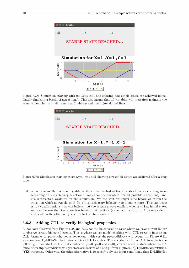
100 6.6. A scenario : a simple network with three variables
Figure 6.38: Simulation starting with x=1,y=1,c=1 and showing how stable states are achieved imme-diately (indicating bassin of attractions). This also means that all variables will thereafter maintain thesame values; that is x will remain at 2 while y and c at 1 (see dotted lines).
Figure 6.39: Simulation starting at x=1,y=1,c=1 and showing how stable states are achieved after a longtime.
6. in fact the oscillation is not stable as it can be reached either in a short term or a long termdepending on the arbitrary selection of values for the variables (for all possible transitions), andthis represents a weakness for the simulation. We can wait for longer time before we attain thetransition which allows the shift from this oscillatory behaviour to a stable state. This can leadsus to two affirmations : we can believe that the system always oscillate when x < 1 at initial state,and also believe that there are two bassin of attractions (either with x=0 or or 1 on one side orwith x=2 on the other side) when in fact we have only 1.
6.6.3 Adding CTL to verify biological propertiesAs we have observed from Figure 6.38 and 6.39, we can be exposed to cases where we have to wait longerto observe certain biological events. This is where we use model checking with CTL to write interestingCTL formulas to prove whether a behaviour (with certain preconditions) will occur. In Figure 6.41,we show how DyMBioNet facilitates writing CTL formulas. The encoded with our CTL formula is thefollowing: if we start with initial conditions (x=0, y=0 and c=0), can we reach a state where x=1 ?.Since, these input conditions will generate oscillations of x and y (from Figure 6.37), DyMBioNet returns a’YES’ response. Otherwise, the other alternative is to specify only the input conditions, then DyMBioNet
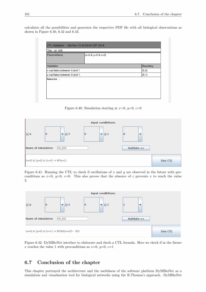
101 6.7. Conclusion of the chapter
calculates all the possibilities and generates the respective PDF file with all biological observations asshown in Figure 6.40, 6.42 and 6.43.
Figure 6.40: Simulation starting at x=0, y=0, c=0
Figure 6.41: Running the CTL to check if oscillations of x and y are observed in the future with pre-conditions as x=0, y=0, c=0. This also proves that the absence of c prevents x to reach the value2.
Figure 6.42: DyMBioNet interface to elaborate and check a CTL formula. Here we check if in the futurex reaches the value 1 with preconditions as x=0, y=0, c=1
6.7 Conclusion of the chapterThis chapter portrayed the architecture and the usefulness of the software platform DyMBioNet as asimulation and visualisation tool for biological networks using the R.Thomas’s approach. DyMBioNet
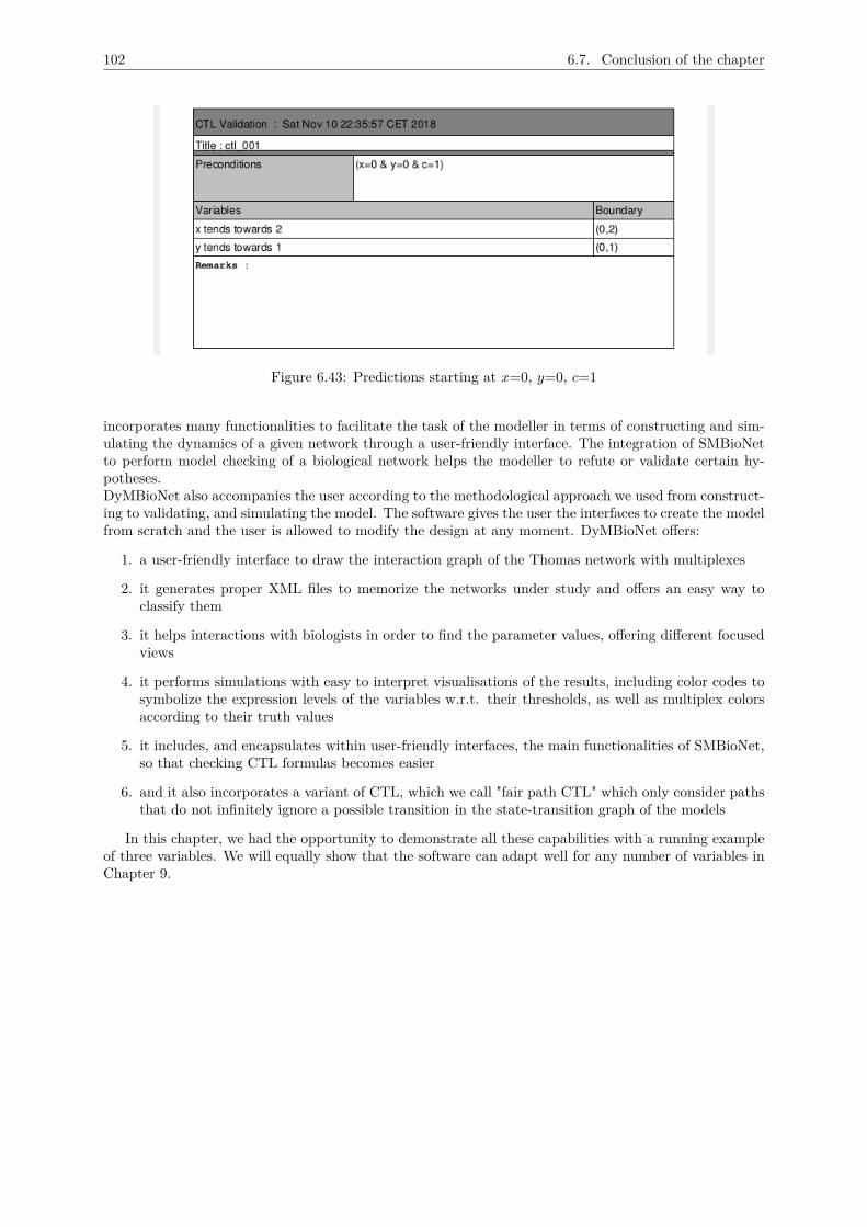
102 6.7. Conclusion of the chapter
Figure 6.43: Predictions starting at x=0, y=0, c=1
incorporates many functionalities to facilitate the task of the modeller in terms of constructing and sim-ulating the dynamics of a given network through a user-friendly interface. The integration of SMBioNetto perform model checking of a biological network helps the modeller to refute or validate certain hy-potheses.DyMBioNet also accompanies the user according to the methodological approach we used from construct-ing to validating, and simulating the model. The software gives the user the interfaces to create the modelfrom scratch and the user is allowed to modify the design at any moment. DyMBioNet offers:
1. a user-friendly interface to draw the interaction graph of the Thomas network with multiplexes
2. it generates proper XML files to memorize the networks under study and offers an easy way toclassify them
3. it helps interactions with biologists in order to find the parameter values, offering different focusedviews
4. it performs simulations with easy to interpret visualisations of the results, including color codes tosymbolize the expression levels of the variables w.r.t. their thresholds, as well as multiplex colorsaccording to their truth values
5. it includes, and encapsulates within user-friendly interfaces, the main functionalities of SMBioNet,so that checking CTL formulas becomes easier
6. and it also incorporates a variant of CTL, which we call "fair path CTL" which only consider pathsthat do not infinitely ignore a possible transition in the state-transition graph of the models
In this chapter, we had the opportunity to demonstrate all these capabilities with a running exampleof three variables. We will equally show that the software can adapt well for any number of variables inChapter 9.
CHAPTER 7ABSTRACT GRAPH FOR THE
REGULATION OF ENERGYMETABOLISM
7.1 IntroductionIn this chapter, we will show the methodology for constructing the abstract model of biological regulationswhich applies not only for gene networks but for metabolic networks as well. We reiterate our question ofinterest which is the regulation of the energy and biomass metabolism. As such, the notion of activatorand inhibitor is adapted by using respectively the notion of "resource consumer" and "resource provider"in order to abstract the underlying mass action rules that governs metabolic fluxes in terms of regulations.We describe here five steps of our methodology (5) which we use to construct our metabolic graph (whichcan be extended to other regulatory graphs) :
1. Inventory of variables with respect to the scientific question and their classification in categories
2. Identification of the biological signals that may influence each target variables mentioned in step1. (Definition of the multiplex, that is a meaningful name for each given biological signal and thegroup of variables that are part of this multiplex).
3. Defining the number of activation states for each variable mentioned in step 1: this is the numberof outgoing arrows emerging from a given variable plus 1 (if counting background state 0).
4. Identifying activating threshold for each interaction between a variable and another variable or amultiplex.
5. Construction of the final graph.
7.2 Inventory of the pertinent variablesTo address the energy and biomass regulations in our study, we categorise four types of variables forcentral carbon metabolism that enter into the description of the respiration-fermentative shift :
1. Metabolic pathways which are subdivided into catabolic and anabolic pathways
2. Molecular cofactors (ATP/ADP, NADH/NAD+)
3. Nutrients (glucose, O2, amino acids and fatty acids) which are subdivided into internal metabolitesand control nutrients
Next, we give the abstract and molecular definition of the variables associated to the four differentclasses.
7.2.1 Metabolic functions and pathwaysFrom our coarse-grained and abstracted view of metabolism, we differentiate two types of metabolicpathways for representing our regulatory graph: catabolism and anabolism. The abstract definitionbelow corresponds to the definition taken by the model. This abstract definition differs from the biologicaldefinition of the variable as at molecular level : a pathway may have many bifurcation points and might
103
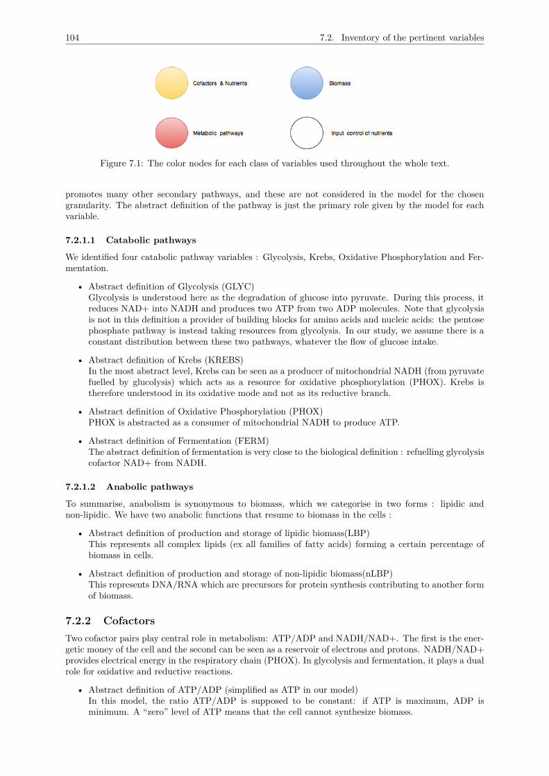
104 7.2. Inventory of the pertinent variables
Figure 7.1: The color nodes for each class of variables used throughout the whole text.
promotes many other secondary pathways, and these are not considered in the model for the chosengranularity. The abstract definition of the pathway is just the primary role given by the model for eachvariable.
7.2.1.1 Catabolic pathways
We identified four catabolic pathway variables : Glycolysis, Krebs, Oxidative Phosphorylation and Fer-mentation.
• Abstract definition of Glycolysis (GLYC)Glycolysis is understood here as the degradation of glucose into pyruvate. During this process, itreduces NAD+ into NADH and produces two ATP from two ADP molecules. Note that glycolysisis not in this definition a provider of building blocks for amino acids and nucleic acids: the pentosephosphate pathway is instead taking resources from glycolysis. In our study, we assume there is aconstant distribution between these two pathways, whatever the flow of glucose intake.
• Abstract definition of Krebs (KREBS)In the most abstract level, Krebs can be seen as a producer of mitochondrial NADH (from pyruvatefuelled by glucolysis) which acts as a resource for oxidative phosphorylation (PHOX). Krebs istherefore understood in its oxidative mode and not as its reductive branch.
• Abstract definition of Oxidative Phosphorylation (PHOX)PHOX is abstracted as a consumer of mitochondrial NADH to produce ATP.
• Abstract definition of Fermentation (FERM)The abstract definition of fermentation is very close to the biological definition : refuelling glycolysiscofactor NAD+ from NADH.
7.2.1.2 Anabolic pathways
To summarise, anabolism is synonymous to biomass, which we categorise in two forms : lipidic andnon-lipidic. We have two anabolic functions that resume to biomass in the cells :
• Abstract definition of production and storage of lipidic biomass(LBP)This represents all complex lipids (ex all families of fatty acids) forming a certain percentage ofbiomass in cells.
• Abstract definition of production and storage of non-lipidic biomass(nLBP)This represents DNA/RNA which are precursors for protein synthesis contributing to another formof biomass.
7.2.2 CofactorsTwo cofactor pairs play central role in metabolism: ATP/ADP and NADH/NAD+. The first is the ener-getic money of the cell and the second can be seen as a reservoir of electrons and protons. NADH/NAD+provides electrical energy in the respiratory chain (PHOX). In glycolysis and fermentation, it plays a dualrole for oxidative and reductive reactions.
• Abstract definition of ATP/ADP (simplified as ATP in our model)In this model, the ratio ATP/ADP is supposed to be constant: if ATP is maximum, ADP isminimum. A “zero” level of ATP means that the cell cannot synthesize biomass.
105 7.3. Identification of regulation signals (metabolism)
• Abstract definition of NADH/NAD+ (simplified as NADH in our model)The NADH/NAD+ corresponds to both cytoplasmic and mitochondrial reduced and oxidized nicoti-namide dinucleotide species. As for ATP/ADP, the ratio NADH/NAD+ is supposed to be constant:if NADH is maximum, NAD+ is minimum. A “zero” level of NADH means that fermentation oroxidative phosphorylation cannot work. A zero level of NAD+ means that glycolysis cannot work.
7.2.3 NutrientsThis section is divided into two parts : nutrients which are internal metabolites and nutrients which actas control variables for the energy metabolic network.
7.2.3.1 Internal metabolites
The cellular regimes for the regulation of the energy metabolism inside cells, called internal metabolites,are Glucose, O2 and Glutamine. They are abstracted as follows:
• Abstract definition of Glucose (GLC)Glucose symbolize the organic matter, i.e. the carbon source, the reservoir of protons and electronsneeded for electric energy production.
• Abstract definition of O2Oxygen is the acceptor of electrons used by the respiratory chain. Absence of oxygen is similar tohypoxic condition and prevents oxidative phosphorylation, and promotes fermentation as an ATPproduction pathway. The shift from respiration to aerobic glycolysis occurs even in presence ofoxygen.
• Abstract definition of nitrogen and carbon donors (NCD)Nitrogen and carbon are essential precursors for the synthesis of amino acids and lipids. A majorityof these nitrogen and carbon skeletons are derived from metabolic processes like glycolysis andKrebs, which we abstract here as NCD.
7.2.3.2 Input variables
In order to control the level of nutrients which are important to mimic cellular environments (like hy-poxia, cancer microenvironment , etc), we use three input variables namely FA to mean Fatty Acids, AAto mean Amino Acids and InO2. We do not have an input for glucose since there are no actions (regu-lations) on glucose in our model. Therefore, glucose (GLC) is both a nutrient as well as an input variable.
Now, that we have the full list of variables, we need to see all the possible interactions between thesevariables to construct the metabolic network, and this is exactly what we will do in the next section.
7.3 Identification of regulation signals (metabolism)The goal of this section is to identify regulation signals or more specifically to distinguish all biologicalregulation signals that influence a given variable of the system. This has to be done for all variablesenumerated in the previous section. This is a preliminary identification as we are only here creating agroup of variables for each regulation signal or regulation mechanism without mentioning at this stagethe state condition of each variable for this regulation signal to occur. It is therefore an inventory of thephenomena that act on that given target variable.
This regulation signal can be triggered by a single variable or by several variables. We suppose thisregulation to act as an on/off signal, for which the target variable switches to another state if in thegroup of variables that form the input signal (the multiplex), each variable is at the required activatedstate. If the notion of a "state" of a variable can yet be defined as its capacity or not to act on anothervariable, it is not possible at the moment to tell how many states a variable may have as it depends onthe number of outgoing arrows in the network, that is on the number of distinct action this variable cando on another (single) variable to change its state.
For illustration, suppose a gene transcript with arbitrary 11 transcript levels numbered 0 to 10. Supposethat this gene transcript induces a single biological regulation signal if it reaches level 5. From levels 5 to10, this gene transcript induces the same effect. This gene transcript has one threshold (corresponding tointernal transcript level 5) which induces two actions: i) doing nothing (inactive state corresponding to
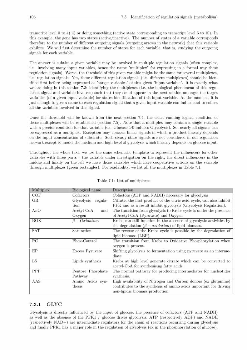
106 7.3. Identification of regulation signals (metabolism)
transcript level 0 to 4) ii) or doing something (active state corresponding to transcript level 5 to 10). Inthis example, the gene has two states (active/inactive). The number of states of a variable correspondstherefore to the number of different outgoing signals (outgoing arrows in the network) that this variableexhibits. We will first determine the number of states for each variable, that is, studying the outgoingsignals for each variable.
The answer is subtle: a given variable may be involved in multiple regulation signals (often complex,i.e. involving many input variables, hence the name "multiplex" for expressing in a formal way theseregulation signals). Worse, the threshold of this given variable might be the same for several multiplexes,i.e. regulation signals. Yet, these different regulation signals (i.e. different multiplexes) should be iden-tified first before being expressed as "target variables" of this given "input variable". It is exactly whatwe are doing in this section 7.3: identifying the multiplexes (i.e. the biological phenomena of this regu-lation signal and variable involves) such that they could appear in the next section amongst the targetvariables (of a given input variable) for states identification of this input variable. At the moment, it isjust enough to give a name to each regulation signal that a given input variable can induce and to collectall the variables involved in this signal.
Once the threshold will be known from the next section 7.4, the exact running logical condition ofthese multiplexes will be established (section 7.5). Note that a multiplex may contain a single variablewith a precise condition for that variable (ex. Glucose >0 induces Glycolysis). So, nearly all signals canbe expressed as a multiplex. Exception may concern linear signals in which a product linearly dependson the input concentration of substrate. Such steady state signals are not considered in our regulationnetwork except to model the medium and high level of glycolysis which linearly depends on glucose input.
Throughout the whole text, we use the same schematic template to represent the influencers for othervariables with three parts : the variable under investigation on the right, the direct influencers in themiddle and finally on the left we have those variables which have cooperative actions on the variablethrough multiplexes (green rectangles). For readability, we list all the multiplexes in Table 7.1.
Table 7.1: List of multiplexes
Multiplex Biological name DescriptionCOF Cofactors Cofactors (ATP and NADH) necessary for glycolysisGR Glycolysis regula-
tionCitrate, the first product of the citric acid cycle, can also inhibitPFK and as a result inhibit glycolysis (Glycolysis Regulation).
AnO Acetyl-CoA andOxygen
The transition from glycolysis to Krebs cycle is under the presenceof Acetyl-CoA (Pyruvate) and Oxygen
BOX β −Oxidation Krebs can still function in the absence of glycolytic activities bythe degradation (β − oxidation) of lipid biomass.
SAT Saturation The reverse of the Krebs cycle is possible by the degradation oflipid biomass (LBP).
PC Phox-Control The transition from Krebs to Oxidative Phosphorylation whenoxygen is present.
EP Excess Pyruvate Shifting glycolysis to fermentation using pyruvate as an interme-diate
LS Lipids synthesis Krebs at high level generate citrate which can be converted toacetyl-CoA for synthesising fatty acids.
PPP Pentose PhosphatePathway
The normal pathway for producing intermediates for nucleotidessynthesis.
AAS Amino Acids syn-thesis
High availability of Nitrogen and Carbon donors (ex glutamine)contributes to the synthesis of amino acids important for drivingnon-lipidic biomass production.
7.3.1 GLYCGlycolysis is directly influenced by the input of glucose, the presence of cofactors (ATP and NADH)as well as the absence of the PFK1 : glucose drives glycolysis, ATP (respectively ADP) and NADH(respectively NAD+) are intermediate regulators for the chain of reactions occurring during glycolysisand finally PFK1 has a major role in the regulation of glycolysis (ex in the phosphorylation of glucose).

107 7.3. Identification of regulation signals (metabolism)
We display these interactions in Figure 7.2.
Figure 7.2: Influencers of glycolysis (GLYC)
7.3.2 KREBSHere, we note two versions of Krebs : an oxidative and normal mode controlled by AnO (Acetyl CoA andoxygen ; that is normal glycolysis) or a reductive mode that can be controlled either by SAT (throughNCD via &-KG) or by the degradation of biomass through BOX (beta-oxidation).
Figure 7.3: Influencers of Krebs (KREBS)
7.3.3 PHOXOxidation phosphorylation occurs only in the presence of oxygen. The sole and direct influencers ofOxidative phosphorylation are oxygen, ATP and NADH whose combined actions are merged in themultiplex PC (Phox-Control in Figure 7.6) as they are all pre-requisites for PHOX to happen.
Figure 7.4: Influencers of Oxidative Phosphorylation (PHOX)
7.3.4 FERMIn our model, fermentation occurs only in the presence of excess pyruvate which results from the combinedaction of three variables : oxygen (its absence triggers fermentation but in the presence of high glucosemilieu, fermentation process can be triggered even in the presence of oxygen), glycolysis (acts as donorof pyruvate) and NADH (see Figure 7.5).
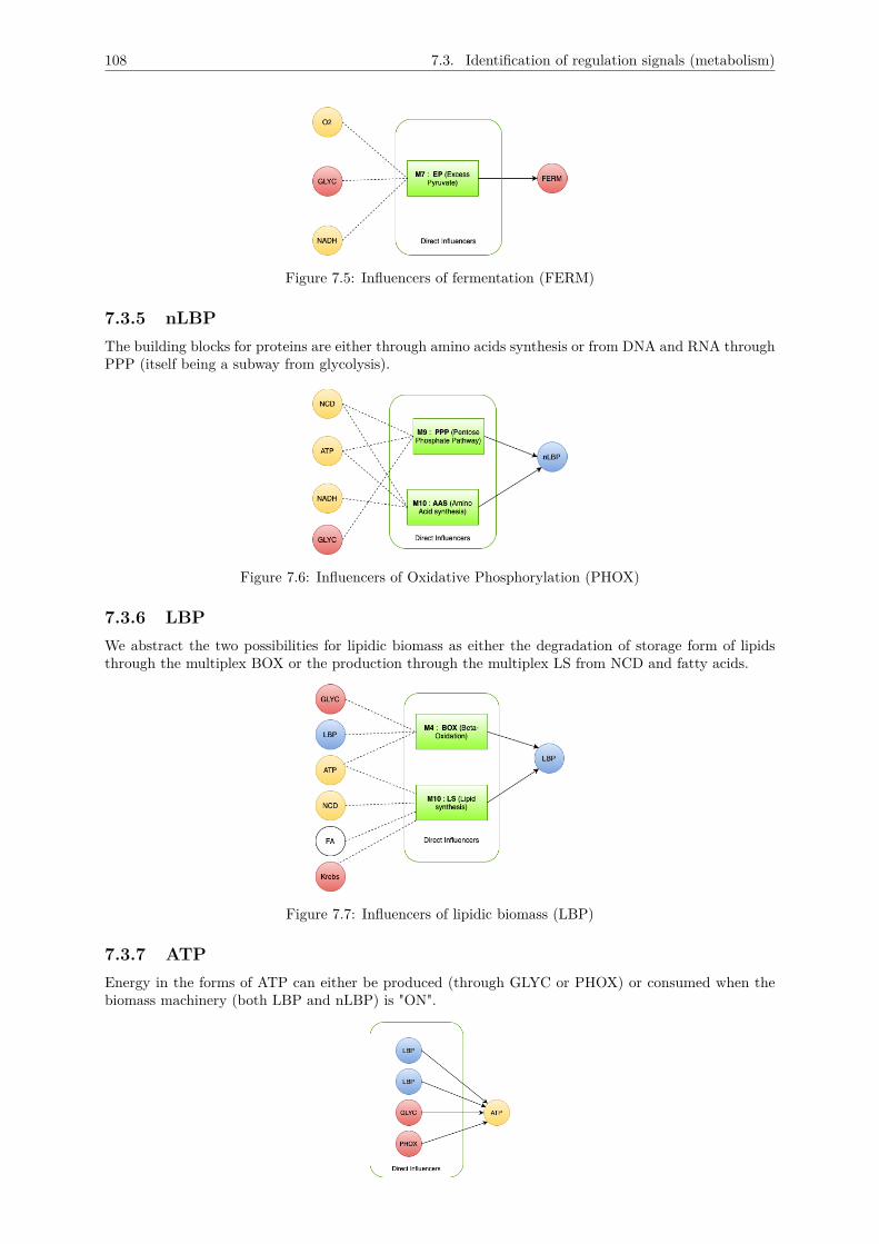
108 7.3. Identification of regulation signals (metabolism)
Figure 7.5: Influencers of fermentation (FERM)
7.3.5 nLBPThe building blocks for proteins are either through amino acids synthesis or from DNA and RNA throughPPP (itself being a subway from glycolysis).
Figure 7.6: Influencers of Oxidative Phosphorylation (PHOX)
7.3.6 LBPWe abstract the two possibilities for lipidic biomass as either the degradation of storage form of lipidsthrough the multiplex BOX or the production through the multiplex LS from NCD and fatty acids.
Figure 7.7: Influencers of lipidic biomass (LBP)
7.3.7 ATPEnergy in the forms of ATP can either be produced (through GLYC or PHOX) or consumed when thebiomass machinery (both LBP and nLBP) is "ON".
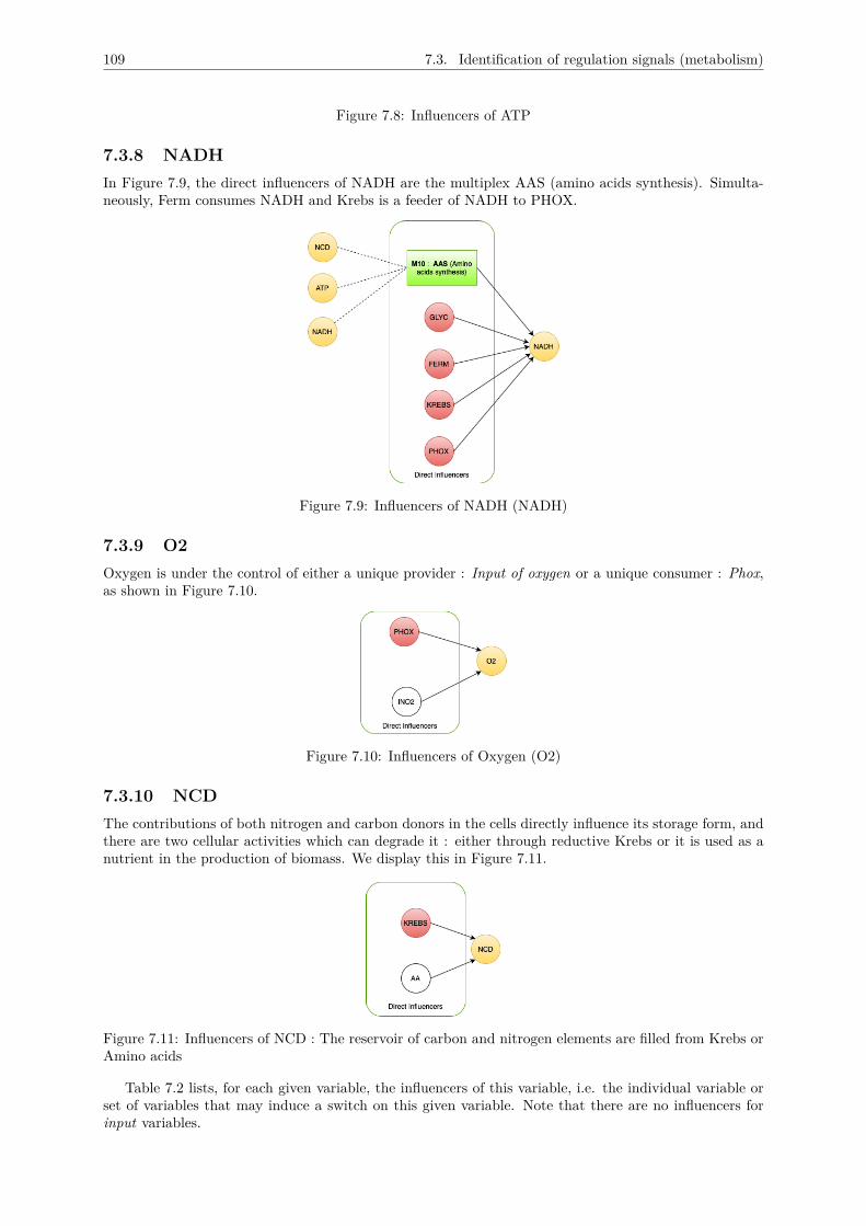
109 7.3. Identification of regulation signals (metabolism)
Figure 7.8: Influencers of ATP
7.3.8 NADHIn Figure 7.9, the direct influencers of NADH are the multiplex AAS (amino acids synthesis). Simulta-neously, Ferm consumes NADH and Krebs is a feeder of NADH to PHOX.
Figure 7.9: Influencers of NADH (NADH)
7.3.9 O2Oxygen is under the control of either a unique provider : Input of oxygen or a unique consumer : Phox,as shown in Figure 7.10.
Figure 7.10: Influencers of Oxygen (O2)
7.3.10 NCDThe contributions of both nitrogen and carbon donors in the cells directly influence its storage form, andthere are two cellular activities which can degrade it : either through reductive Krebs or it is used as anutrient in the production of biomass. We display this in Figure 7.11.
Figure 7.11: Influencers of NCD : The reservoir of carbon and nitrogen elements are filled from Krebs orAmino acids
Table 7.2 lists, for each given variable, the influencers of this variable, i.e. the individual variable orset of variables that may induce a switch on this given variable. Note that there are no influencers forinput variables.
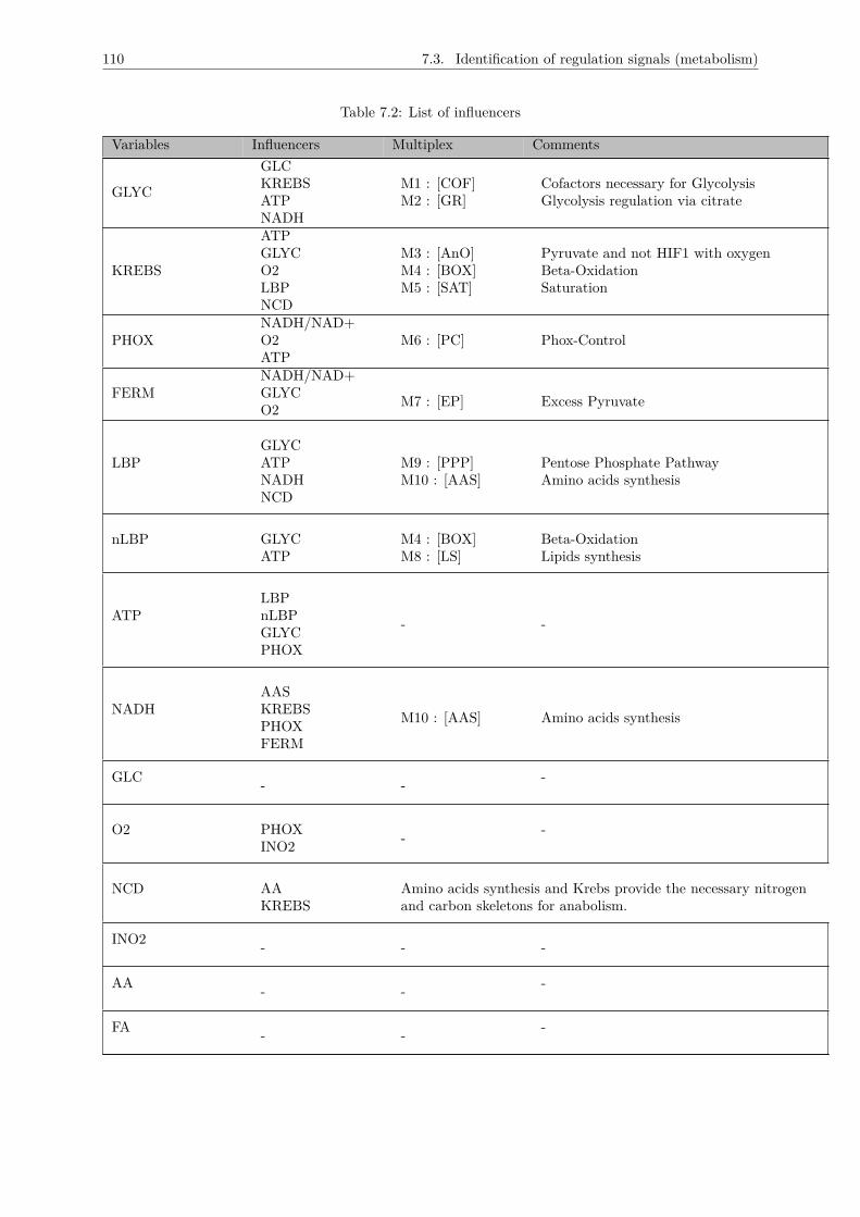
110 7.3. Identification of regulation signals (metabolism)
Table 7.2: List of influencers
Variables Influencers Multiplex Comments
GLYC
GLCKREBSATPNADH
M1 : [COF]M2 : [GR]
Cofactors necessary for GlycolysisGlycolysis regulation via citrate
KREBS
ATPGLYCO2LBPNCD
M3 : [AnO]M4 : [BOX]M5 : [SAT]
Pyruvate and not HIF1 with oxygenBeta-OxidationSaturation
PHOXNADH/NAD+O2ATP
M6 : [PC] Phox-Control
FERMNADH/NAD+GLYCO2 M7 : [EP] Excess Pyruvate
LBPGLYCATPNADHNCD
M9 : [PPP]M10 : [AAS]
Pentose Phosphate PathwayAmino acids synthesis
nLBP GLYCATP
M4 : [BOX]M8 : [LS]
Beta-OxidationLipids synthesis
ATPLBPnLBPGLYCPHOX
- -
NADHAASKREBSPHOXFERM
M10 : [AAS] Amino acids synthesis
GLC - - -
O2 PHOXINO2 - -
NCD AAKREBS
Amino acids synthesis and Krebs provide the necessary nitrogenand carbon skeletons for anabolism.
INO2 - - -
AA - - -
FA - - -
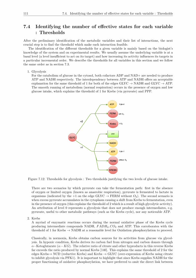
111 7.4. Identifying the number of effective states for each variable : Thresholds
7.4 Identifying the number of effective states for each variable: Thresholds
After the preliminary identification of the metabolic variables and their list of interactions, the nextcrucial step is to find the threshold which make each interaction feasible.
The identification of the different thresholds for a given variable is mainly based on the biologist’sknowledge of the system and on experimental results. We usually assume the underlying variable is at abasal level (a level insufficient to act on its target) and how increasing its activity influences its targets ina particular incremental order. We describe the thresholds for all variables in this section and we followthe same order as in section 7.3.
1. GlycolysisFor the catabolism of glucose in the cytosol, both cofactors ADP and NAD+ are needed to produceATP and NADH respectively. The interdependency between ATP and NADH offers an acceptableexplanation for the same threshold of 1 for both of the edges GLYC → NADH and GLYC → ATP.The smooth running of metabolism (normal respiration) occurs in the presence of oxygen and lowglucose intake, which explains the threshold of 1 for Krebs (via pyruvate) and PPP.
Figure 7.12: Thresholds for glycolysis : Two thresholds justifying the two levels of glucose intake.
There are two scenarios by which pyruvate can take the fermentation path: first in the absenceof oxygen or limited oxygen (known as anaerobic respiration), pyruvate is fermented to lactate inorganisms (indicated by the +1 on the edge GLYC → FERM without O2). The second scenario iswhen excess pyruvate accumulates in the cytoplasm causing a shift from Krebs to fermentation, evenin the presence of oxygen (this explains the threshold of 2 which is a result of high glycolytic activity).An attribution of level 0 represents a glycolysis that does not produce enough intermediates, e.g.pyruvate, useful to other metabolic pathways (such as the Krebs cycle), nor any noticeable ATP.
2. KrebsA myriad of enzymatic reactions occurs during the normal oxidative phase of the Krebs cycleproducing intermediate compounds NADH, FADH2, CO2 and ATP. This corroborates with thethreshold of 1 for Krebs → NADH at a reasonable level for Oxidation phosphorylation to proceed.
Classically, in normoxia, Krebs obtains carbon sources for its activities from glucose via glycol-ysis. In hypoxic condition, Krebs derives its carbon fuel from nitrogen and carbon donors throughα−Ketoglutarate (α−KG). The relative ratio of citrate and other byproducts in this reverse Krebsfar exceeds the ratio produced by normal Krebs [140]. This explains the same threshold of 2 for theedges Krebs→ NCD (reductive Krebs) and Krebs → GLYC (over-expression of Krebs using citrateto inhibit glycolysis via PFK1). It is important to highlight that since Krebs supplies NADH for theproper functioning of oxidative phosphorylation, we have preferred to omit the direct link between
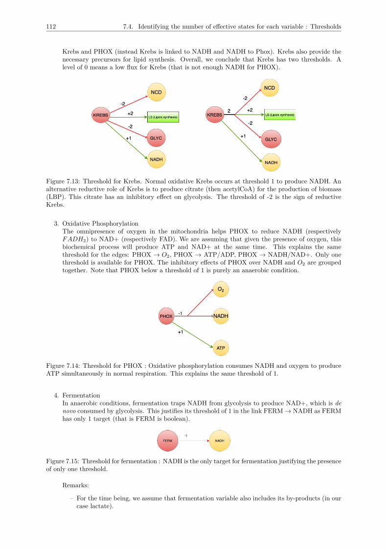
112 7.4. Identifying the number of effective states for each variable : Thresholds
Krebs and PHOX (instead Krebs is linked to NADH and NADH to Phox). Krebs also provide thenecessary precursors for lipid synthesis. Overall, we conclude that Krebs has two thresholds. Alevel of 0 means a low flux for Krebs (that is not enough NADH for PHOX).
Figure 7.13: Threshold for Krebs. Normal oxidative Krebs occurs at threshold 1 to produce NADH. Analternative reductive role of Krebs is to produce citrate (then acetylCoA) for the production of biomass(LBP). This citrate has an inhibitory effect on glycolysis. The threshold of -2 is the sign of reductiveKrebs.
3. Oxidative PhosphorylationThe omnipresence of oxygen in the mitochondria helps PHOX to reduce NADH (respectivelyFADH2) to NAD+ (respectively FAD). We are assuming that given the presence of oxygen, thisbiochemical process will produce ATP and NAD+ at the same time. This explains the samethreshold for the edges: PHOX → O2, PHOX → ATP/ADP, PHOX → NADH/NAD+. Only onethreshold is available for PHOX. The inhibitory effects of PHOX over NADH and O2 are groupedtogether. Note that PHOX below a threshold of 1 is purely an anaerobic condition.
Figure 7.14: Threshold for PHOX : Oxidative phosphorylation consumes NADH and oxygen to produceATP simultaneously in normal respiration. This explains the same threshold of 1.
4. FermentationIn anaerobic conditions, fermentation traps NADH from glycolysis to produce NAD+, which is denovo consumed by glycolysis. This justifies its threshold of 1 in the link FERM→ NADH as FERMhas only 1 target (that is FERM is boolean).
Figure 7.15: Threshold for fermentation : NADH is the only target for fermentation justifying the presenceof only one threshold.
Remarks:
– For the time being, we assume that fermentation variable also includes its by-products (in ourcase lactate).
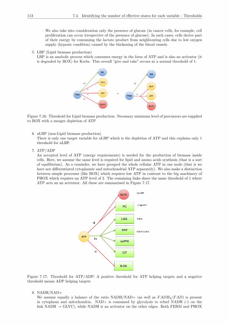
113 7.4. Identifying the number of effective states for each variable : Thresholds
– We also take into consideration only the presence of glucose (in cancer cells, for example, cellproliferation can occur irrespective of the presence of glucose). In such cases, cells derive partof their energy by consuming the lactate product from neighbouring cells due to low oxygensupply (hypoxic condition) caused by the thickening of the blood vessels.
5. LBP (Lipid biomass production)LBP is an anabolic process which consumes energy in the form of ATP and is also an activator (itis degraded by BOX) for Krebs. This overall "give and take" occurs at a normal threshold of 1.
Figure 7.16: Threshold for Lipid biomass production: Necessary minimum level of precursors are suppliedto BOX with a meagre depletion of ATP
6. nLBP (non-Lipid biomass production)There is only one target variable for nLBP which is the depletion of ATP and this explains only 1threshold for nLBP.
7. ATP/ADPAn accepted level of ATP (energy requirements) is needed for the production of biomass insidecells. Here, we assume the same level is required for lipid and amino acids synthesis (that is a sortof equilibrium). As a reminder, we have grouped the whole cellular ATP in one node (that is wehave not differentiated cytoplasmic and mitochondrial ATP separately). We also make a distinctionbetween simple processes (like BOX) which requires low ATP in contrast to the big machinery ofPHOX which requires an ATP level of 2. The remaining links share the same threshold of 1 whereATP acts an an activator. All these are summarised in Figure 7.17.
Figure 7.17: Threshold for ATP/ADP: A positive threshold for ATP helping targets and a negativethreshold means ADP helping targets
8. NADH/NAD+We assume equally a balance of the ratio NADH/NAD+ (as well as FADH2/FAD) is presentin cytoplasm and mitochondria. NAD+ is consumed by glycolysis to refuel NADH (-1 on thelink NADH → GLYC), while NADH is an activator on the other edges. Both FERM and PHOX
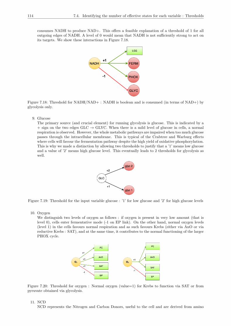
114 7.4. Identifying the number of effective states for each variable : Thresholds
consumes NADH to produce NAD+. This offers a feasible explanation of a threshold of 1 for alloutgoing edges of NADH. A level of 0 would mean that NADH is not sufficiently strong to act onits targets. We show these interactions in Figure 7.18.
Figure 7.18: Threshold for NADH/NAD+ : NADH is boolean and is consumed (in terms of NAD+) byglycolysis only.
9. GlucoseThe primary source (and crucial element) for running glycolysis is glucose. This is indicated by a+ sign on the two edges GLC → GLYC. When there is a mild level of glucose in cells, a normalrespiration is observed. However, the whole metabolic pathways are impaired when too much glucosepasses through the intracellular membrane. This is typical of the Crabtree and Warburg effectswhere cells will favour the fermentation pathway despite the high yield of oxidative phosphorylation.This is why we made a distinction by allowing two thresholds to justify that a ’1’ means low glucoseand a value of ’2’ means high glucose level. This eventually leads to 2 thresholds for glycolysis aswell.
Figure 7.19: Threshold for the input variable glucose : ’1’ for low glucose and ’2’ for high glucose levels
10. OxygenWe distinguish two levels of oxygen as follows : if oxygen is present in very low amount (that islevel 0), cells enter fermentative mode (-1 on EP link). On the other hand, normal oxygen levels(level 1) in the cells favours normal respiration and as such favours Krebs (either via AnO or viareductive Krebs : SAT), and at the same time, it contributes to the normal functioning of the largerPHOX cycle.
Figure 7.20: Threshold for oxygen : Normal oxygen (value=1) for Krebs to function via SAT or frompyruvate obtained via glycolysis.
11. NCDNCD represents the Nitrogen and Carbon Donors, useful to the cell and are derived from amino

115 7.5. Logical description of the multiplexes
acids (AA). These donors are precursors for many anabolic activities : at level 0 NCD action is toolow to undergo anabolic processes; at level 1 it can participate to the activation of the PPP; whileat level 2, it contributes to intensive anabolic activities like lipid synthesis (LS) and AAS (aminoacids synthesis) and also fuels reductive Krebs.
Figure 7.21: Thresholds for NCD : Nitrogen and carbon skeletons are important for almost all anabolicactivities. A level of 0 means its inactive state.
12. FA, AA and InO2The input or environmental variables, namely fatty acids, amino acids and oxygen, refer to theabstract level of nutrients we consider important for metabolic processes, and they play vital rolesin the study of Warburg/Crabtree effect. FA and InO2 are both boolean variables simulatingdifferent cell’s milieu. We differentiate 2 levels for AA since we consider its contribution to lipidand amino acids synthesis varies.
7.5 Logical description of the multiplexesAs a reminder from chapter 5, we distinguished two types of multiplexes : implicit (where there is onlyone atom and no biological significance in our model) and explicit (where there are at least two atomsinfluencing the target variables). In this section, we first list all the explicit multiplexes in the same orderas described in Table 7.2.
• M1 - [COF] : ¬(ATP ≥ 2) ∧ ¬(NADH ≥ 1)The multiplex COF, which refers to cofactors, gives the minimal condition necessary to inducenormal glycolysis:
Hypothesis: As soon as there is ADP and NAD+, the glycolysis is working at normal rate.
Figure 7.22: ADP (!ATP) and NAD+(!NADH) are both important cofactors required for glycolysis.
• M2 - [GR] : ¬[(KREBS ≥ 2) ∧ (ATP ≥ 1)]The multiplex GR gives the condition to inhibit glycolysis by ATP (ATP ≥ 1) meaning also theabsence of PFK (Phospho-fructo-kinase) and an accumulation of citrate. Moreover, the end productof glycolysis (pyruvate) fuels the TCA cycle and is transformed into citrate, which, if in excess,inhibits glycolysis. So, GLYC is inhibited when both conditions are satisfied as indicated in themultiplex formula.
• M3 - [AnO] : (GLY C ≥ 1) ∧ (O2 ≥ 1)A variety of glucose transporters (GLUT1 to GLUT5) are available to facilitate the entry of glucosemolecules through the cell membrane [149]. Under normal conditions (glyc >= 1), glucose isconverted to pyruvate which in turns is converted to acetyl-CoA in the presence of oxygen (O2 >=1). Pyruvate molecules are then used to continue the Krebs cycle which is the second step of aerobicglycolysis.
• M4 - [BOX] : (BM ≥ 1) ∧ ¬(GLY C ≥ 1) ∧ ¬(ATP ≥ 1)In conditions of glucose deprivation !(glyc >= 1), cells undergo a catabolic process during which
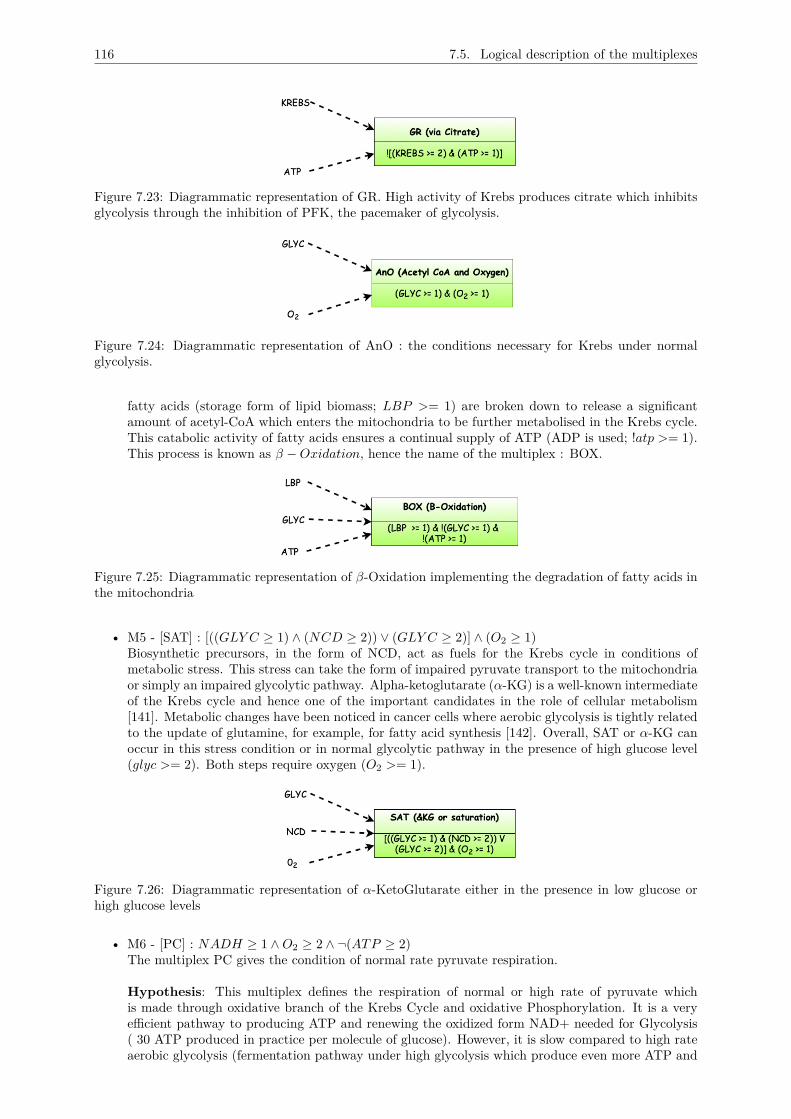
116 7.5. Logical description of the multiplexes
Figure 7.23: Diagrammatic representation of GR. High activity of Krebs produces citrate which inhibitsglycolysis through the inhibition of PFK, the pacemaker of glycolysis.
Figure 7.24: Diagrammatic representation of AnO : the conditions necessary for Krebs under normalglycolysis.
fatty acids (storage form of lipid biomass; LBP >= 1) are broken down to release a significantamount of acetyl-CoA which enters the mitochondria to be further metabolised in the Krebs cycle.This catabolic activity of fatty acids ensures a continual supply of ATP (ADP is used; !atp >= 1).This process is known as β −Oxidation, hence the name of the multiplex : BOX.
Figure 7.25: Diagrammatic representation of β-Oxidation implementing the degradation of fatty acids inthe mitochondria
• M5 - [SAT] : [((GLY C ≥ 1) ∧ (NCD ≥ 2)) ∨ (GLY C ≥ 2)] ∧ (O2 ≥ 1)Biosynthetic precursors, in the form of NCD, act as fuels for the Krebs cycle in conditions ofmetabolic stress. This stress can take the form of impaired pyruvate transport to the mitochondriaor simply an impaired glycolytic pathway. Alpha-ketoglutarate (α-KG) is a well-known intermediateof the Krebs cycle and hence one of the important candidates in the role of cellular metabolism[141]. Metabolic changes have been noticed in cancer cells where aerobic glycolysis is tightly relatedto the update of glutamine, for example, for fatty acid synthesis [142]. Overall, SAT or α-KG canoccur in this stress condition or in normal glycolytic pathway in the presence of high glucose level(glyc >= 2). Both steps require oxygen (O2 >= 1).
Figure 7.26: Diagrammatic representation of α-KetoGlutarate either in the presence in low glucose orhigh glucose levels
• M6 - [PC] : NADH ≥ 1 ∧O2 ≥ 2 ∧ ¬(ATP ≥ 2)The multiplex PC gives the condition of normal rate pyruvate respiration.
Hypothesis: This multiplex defines the respiration of normal or high rate of pyruvate whichis made through oxidative branch of the Krebs Cycle and oxidative Phosphorylation. It is a veryefficient pathway to producing ATP and renewing the oxidized form NAD+ needed for Glycolysis( 30 ATP produced in practice per molecule of glucose). However, it is slow compared to high rateaerobic glycolysis (fermentation pathway under high glycolysis which produce even more ATP and
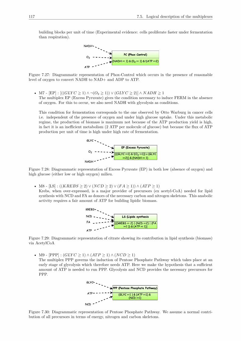
117 7.5. Logical description of the multiplexes
building blocks per unit of time (Experimental evidence: cells proliferate faster under fermentationthan respiration).
Figure 7.27: Diagrammatic representation of Phox-Control which occurs in the presence of reasonablelevel of oxygen to convert NADH to NAD+ and ADP to ATP.
• M7 - [EP] : [((GLY C ≥ 1) ∧ ¬(O2 ≥ 1)) ∨ (GLY C ≥ 2)] ∧NADH ≥ 1The multiplex EP (Excess Pyruvate) gives the condition necessary to induce FERM in the absenceof oxygen. For this to occur, we also need NADH with glycolysis as conditions.
This condition for fermentation corresponds to the one observed by Otto Warburg in cancer cellsi.e. independent of the presence of oxygen and under high glucose uptake. Under this metabolicregime, the production of biomass is maximum not because of the ATP production yield is high,in fact it is an inefficient metabolism (2 ATP per molecule of glucose) but because the flux of ATPproduction per unit of time is high under high rate of fermentation.
Figure 7.28: Diagrammatic representation of Excess Pyruvate (EP) in both low (absence of oxygen) andhigh glucose (either low or high oxygen) milieu.
• M8 - [LS] : ((KREBS ≥ 2) ∨ (NCD ≥ 2) ∨ (FA ≥ 1)) ∧ (ATP ≥ 1)Krebs, when over-expressed, is a major provider of precursors (ex acetyl-CoA) needed for lipidsynthesis with NCD and FA as donors of the necessary carbon and nitrogen skeletons. This anabolicactivity requires a fair amount of ATP for building lipidic biomass.
Figure 7.29: Diagrammatic representation of citrate showing its contribution in lipid synthesis (biomass)via AcetylCoA
• M9 - [PPP] : (GLY C ≥ 1) ∧ (ATP ≥ 1) ∧ (NCD ≥ 1)The multiplex PPP governs the induction of Pentose Phosphate Pathway which takes place at anearly stage of glycolysis which therefore needs ATP. Here we make the hypothesis that a sufficientamount of ATP is needed to run PPP. Glycolysis and NCD provides the necessary precursors forPPP.
Figure 7.30: Diagrammatic representation of Pentose Phosphate Pathway. We assume a normal contri-bution of all precursors in terms of energy, nitrogen and carbon skeletons.
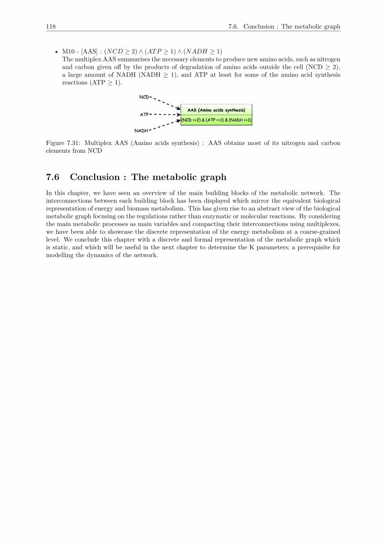
118 7.6. Conclusion : The metabolic graph
• M10 - [AAS] : (NCD ≥ 2) ∧ (ATP ≥ 1) ∧ (NADH ≥ 1)The multiplex AAS summarises the necessary elements to produce new amino acids, such as nitrogenand carbon given off by the products of degradation of amino acids outside the cell (NCD ≥ 2),a large amount of NADH (NADH ≥ 1), and ATP at least for some of the amino acid synthesisreactions (ATP ≥ 1).
Figure 7.31: Multiplex AAS (Amino acids synthesis) : AAS obtains most of its nitrogen and carbonelements from NCD
7.6 Conclusion : The metabolic graphIn this chapter, we have seen an overview of the main building blocks of the metabolic network. Theinterconnections between each building block has been displayed which mirror the equivalent biologicalrepresentation of energy and biomass metabolism. This has given rise to an abstract view of the biologicalmetabolic graph focusing on the regulations rather than enzymatic or molecular reactions. By consideringthe main metabolic processes as main variables and compacting their interconnections using multiplexes,we have been able to showcase the discrete representation of the energy metabolism at a coarse-grainedlevel. We conclude this chapter with a discrete and formal representation of the metabolic graph whichis static, and which will be useful in the next chapter to determine the K parameters; a prerequisite formodelling the dynamics of the network.
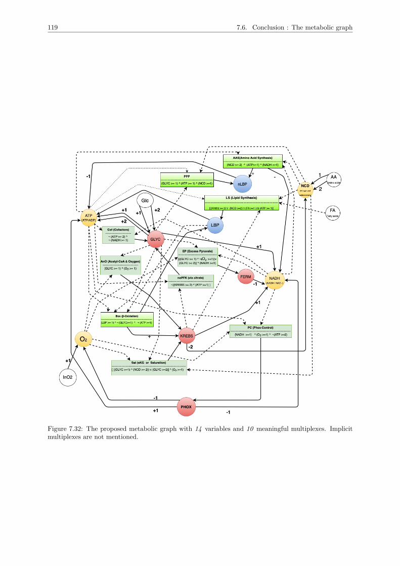
119 7.6. Conclusion : The metabolic graph
Figure 7.32: The proposed metabolic graph with 14 variables and 10 meaningful multiplexes. Implicitmultiplexes are not mentioned.
CHAPTER 8RELATIVE FORCES BETWEENBIOLOGICAL REGULATIONS :
k-PARAMETERS
8.1 IntroductionThe purpose of this chapter is to identify the kinetic parameters for each variable with biological expla-nation according to each possible set of resources and following the methodology defined in Chapter 5(Section 5). To better understand regulations and consequently the dynamics of a biological network,one first needs to do an inventory of all the active regulations for each variable in the network and thechallenge is to get the value towards which each variable tends to evolve, based on the input signals(or active regulations) it receives. This value is influenced by the activation of the regulators or moreprecisely the multiplexes (i.e set of multiplexes) acting on the said variable. A multiplex is active whenits formula is true or inactive if false. Remind that the influencers on a variable can be activators andinhibitors : an inhibitor is active when its formula is false, and as such the formula for an inhibitor ispreceded by a ¬ sign (negation). Finally, if there are n input arrows to a given target variable, there willbe 2n possible combination of active resources.It is a small chapter but it contains a considerable amount of interdisciplinary works between modellersand biologists or biochemists.
For sake of clarity, we will present the K parameters in always the same three steps:
a) eliminate those kinetic parameters where we have contradictions. This can occur in two main cases :first, a variable which passes threshold n must also pass all lower thresholds, and second, a multiplexcontaining the logical formula of another multiplex cannot occur without the latter multiplex. Thishelps us to eliminate those parameters which are useless because there is no state of the systemwhere they apply.
b) list all kinetic parameters which have 0 values based on the availability of resources.
c) list all kinetic parameters which have values other than 0
We do not apply these steps to variables that have only one resource as it is logical that in the absenceof the resource, the value will be 0; otherwise, the value of the K parameter will have the maximumthreshold value of the variable : else, it would mean that the interaction graph contains interactions thatare never functional.
8.2 Identification of the K parametersMost of the K parameters have obvious value due to simple facts such as "no resource, no product".The extraction of these K parameters is based on biological literature or parameter values from publicdatabases (e.g. the Km of an enzyme inhibitor).Nevertheless, new discovery or unknown experimental facts from us might lead to reconsider certain ofthese parameter values (but currently, the model is correct with respect to our knowledge).
In this chapter, the template used in the identification of parameters are : on the left we have solid
120
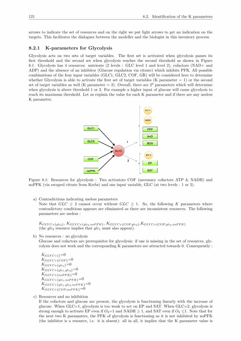
121 8.2. Identification of the K parameters
arrows to indicate the set of resources and on the right we put light arrows to get an indication on thetargets. This facilitates the dialogues between the modeller and the biologist in this inventory process.
8.2.1 K-parameters for GlycolysisGlycolysis acts on two sets of target variables. The first set is activated when glycolysis passes itsfirst threshold and the second set when glycolysis reaches the second threshold as shown in Figure8.1. Glycolysis has 4 resources: nutrients (2 levels : GLC level 1 and level 2), cofactors (NAD+ andADP) and the absence of an inhibitor (Glucose regulation via citrate) which inhibits PFK. All possiblecombinations of the four input variables (GLC1, GLC2, COF, GR) will be considered here to determinewhether Glycolysis is able to activate the first set of target variables (K parameter = 1) or the secondset of target variables as well (K parameter = 2). Overall, there are 24 parameters which will determinewhen glycolysis is above threshold 1 or 2. For example a higher input of glucose will cause glycolysis toreach its maximum threshold. Let us explain the value for each K parameter and if there are any uselessK parameter.
Figure 8.1: Resources for glycolysis : Two activators COF (necessary cofactors ATP & NADH) andnoPFK (via escaped citrate from Krebs) and one input variable, GLC (at two levels : 1 or 2).
a) Contradictions indicating useless parametersNote that GLC ≥ 2 cannot occur without GLC ≥ 1. So, the following K parameters wherecontradictory conditions appears are eliminated as there are inconsistent resources. The followingparameters are useless :
KGLY C+{glc2}, KGLY C+{glc2,noP F K}, KGLY C+{COF,glc2},KGLY C+{COF,glc2,noP F K}(the glc2 resource implies that glc1 must also appear).
b) No resources : no glycolysisGlucose and cofactors are prerequisites for glycolysis: if one is missing in the set of resources, gly-colysis does not work and the corresponding K parameters are attracted towards 0. Consequently :
KGLY C+{}=0KGLY C+{COF}=0KGLY C+{glc1}=0KGLY C+{glc1,glc2}=0KGLY C+{noP F K}=0KGLY C+{glc1,noP F K}=0KGLY C+{glc1,glc2,noP F K}=0KGLY C+{COF,noP F K}=0
c) Resources and no inhibitionIf the cofactors and glucose are present, the glycolysis is functioning linearly with the increase ofglucose. When GLC=1, glycolysis is too weak to act on EP and SAT. When GLC=2, glycolysis isstrong enough to activate EP even if O2=1 and NADH ≥ 1, and SAT even if O2 ≤1. Note that forthe next two K paramaters, the PFK of glycolysis is functioning as it is not inhibited by noPFK(the inhibitor is a resource, i.e. it is absent): all in all, it implies that the K parameter value is
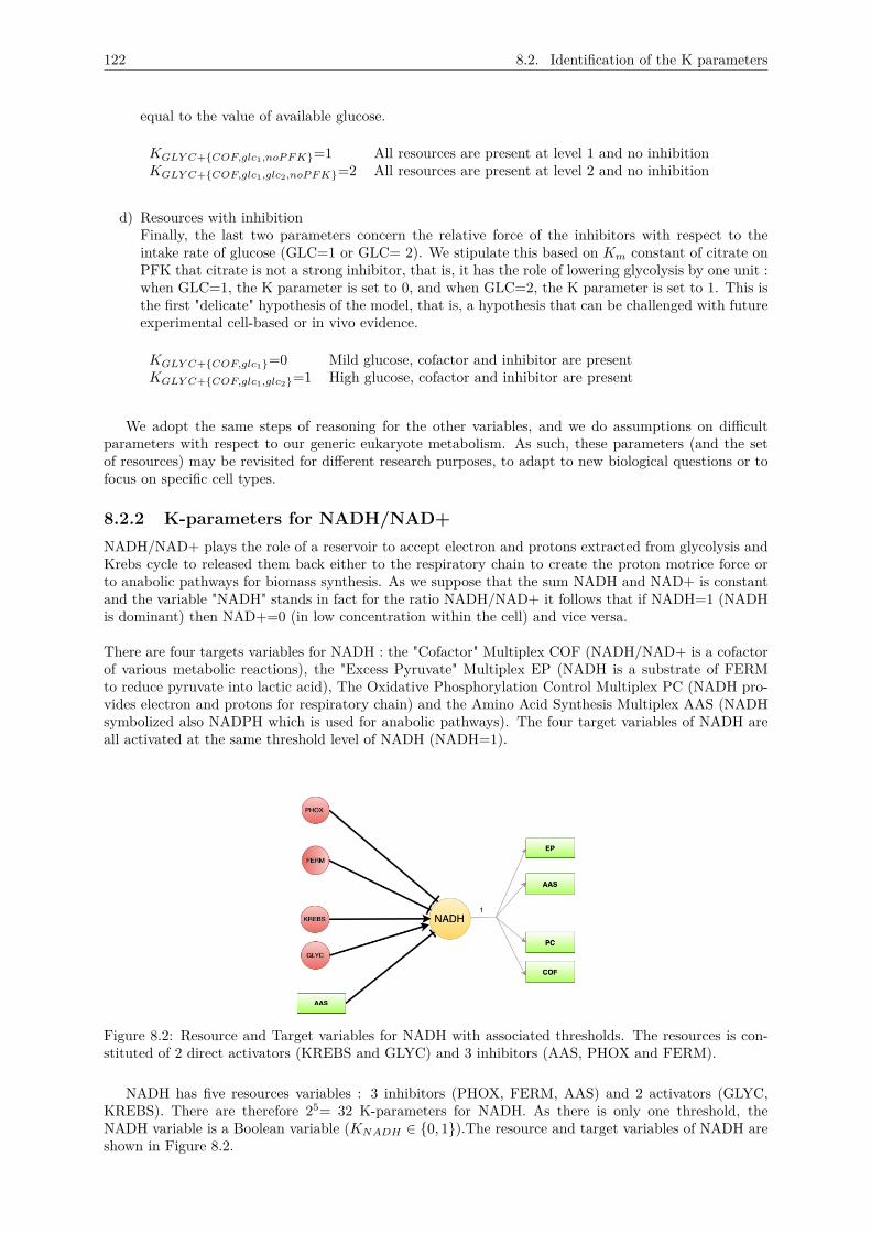
122 8.2. Identification of the K parameters
equal to the value of available glucose.
KGLY C+{COF,glc1,noP F K}=1 All resources are present at level 1 and no inhibitionKGLY C+{COF,glc1,glc2,noP F K}=2 All resources are present at level 2 and no inhibition
d) Resources with inhibitionFinally, the last two parameters concern the relative force of the inhibitors with respect to theintake rate of glucose (GLC=1 or GLC= 2). We stipulate this based on Km constant of citrate onPFK that citrate is not a strong inhibitor, that is, it has the role of lowering glycolysis by one unit :when GLC=1, the K parameter is set to 0, and when GLC=2, the K parameter is set to 1. This isthe first "delicate" hypothesis of the model, that is, a hypothesis that can be challenged with futureexperimental cell-based or in vivo evidence.
KGLY C+{COF,glc1}=0 Mild glucose, cofactor and inhibitor are presentKGLY C+{COF,glc1,glc2}=1 High glucose, cofactor and inhibitor are present
We adopt the same steps of reasoning for the other variables, and we do assumptions on difficultparameters with respect to our generic eukaryote metabolism. As such, these parameters (and the setof resources) may be revisited for different research purposes, to adapt to new biological questions or tofocus on specific cell types.
8.2.2 K-parameters for NADH/NAD+NADH/NAD+ plays the role of a reservoir to accept electron and protons extracted from glycolysis andKrebs cycle to released them back either to the respiratory chain to create the proton motrice force orto anabolic pathways for biomass synthesis. As we suppose that the sum NADH and NAD+ is constantand the variable "NADH" stands in fact for the ratio NADH/NAD+ it follows that if NADH=1 (NADHis dominant) then NAD+=0 (in low concentration within the cell) and vice versa.
There are four targets variables for NADH : the "Cofactor" Multiplex COF (NADH/NAD+ is a cofactorof various metabolic reactions), the "Excess Pyruvate" Multiplex EP (NADH is a substrate of FERMto reduce pyruvate into lactic acid), The Oxidative Phosphorylation Control Multiplex PC (NADH pro-vides electron and protons for respiratory chain) and the Amino Acid Synthesis Multiplex AAS (NADHsymbolized also NADPH which is used for anabolic pathways). The four target variables of NADH areall activated at the same threshold level of NADH (NADH=1).
Figure 8.2: Resource and Target variables for NADH with associated thresholds. The resources is con-stituted of 2 direct activators (KREBS and GLYC) and 3 inhibitors (AAS, PHOX and FERM).
NADH has five resources variables : 3 inhibitors (PHOX, FERM, AAS) and 2 activators (GLYC,KREBS). There are therefore 25= 32 K-parameters for NADH. As there is only one threshold, theNADH variable is a Boolean variable (KNADH ∈ {0, 1}).The resource and target variables of NADH areshown in Figure 8.2.
123 8.2. Identification of the K parameters
The determination of the K-parameters relies on hypotheses that stipulates relative force between con-tradictory signals, i.e. inhibiting and activating signals. These hypotheses correspond in fact to statusof the cell (e.g. proliferative versus quiescence mode). The hypotheses are therefore adapted to the typeof cell we want to consider in the model. The hypotheses below correspond to a normal cell without theglycolytic phenotype.
Hypothesis 1: PHOX consumption of NADH balance the NADH production of KREBS (normaloxidative direction of KREBS). When such oxidative KREBS is functioning, it include NADH producedby glycolysis in low or medium mode, i.e. when GLYC ≤1. PHOX therefore does not balance KREBS+ GLYC when GLYC is at high level (glycolytic phenotype). So when KREBS is present with GLYC,then GLYC is supposed to be weak and PHOX consumes all NADH produced by KREBS and GLYC.
Hypothesis 2: when KREBS and GLYC are present, KREBS produces more NADH than GLYCwhich is suppose to be weak in the respiratory metabolism. So the consideration of these relative forcesrelies not on time but on yield (number of NADH produced per molecule of glucose consumed).
Hypothesis 3: Inhibition of NADH by PHOX is stronger than inhibition by FERM. This is an hy-pothesis which is difficult to check experimentally from a metabolic flux point of view. Instead it can bechecked more easily through indirect incidence of phenotype (see validation techniques of cell phenotypesin the next chapter).
Hypothesis 4: In a proliferative mode whether in respiratory or fermentative metabolism, cell willtend to produce biomass and the anabolic processes (AAS multiplex) may be considered as a big con-sumer of NADH. (This might not be the case for quiescent cells). We suppose therefore that AAS isa stronger consumer of NADH than FERM. AAS is therefore equivalent to PHOX in terms of NADHconsumption.
We identify all parameters starting with the most obvious considerations, i.e. absence of providersfollowed by the presence of providers only. The following 21 descriptors are further identified into twosteps depending on whether anabolic pathways (AAS) are taken into account or not.
a) No providersThere are 8 K parameters falling in this case. There are all set to the value 0.KNADH+{}=0 (no resources)KNADH+{P HOX}=0 (PHOX consumer is absent)KNADH+{F ERM}=0 (FERM consumer is absent)KNADH+{AAS}=0 (AAS consumer is absent)KNADH+{F ERM,P HOX}=0 (PHOX & FERM consumers are absent)KNADH+{F ERM,AAS}=0 (FERM & AAS consumers are absent)KNADH+{P HOX,AAS}=0 (PHOX & AAS consumers are absent)KNADH+{F ERM,P HOX,AAS}=0 (PHOX & AAS consumers are absent)
We are left with 32 - 8 = 24 parameters to find.
b) No consumers - one provider at leastThe second subset of parameters concerns those for which there is no consumer and at least oneprovider in the combination of resources. There are 3 K parameters in this case, all set to themaximum value 1.KNADH+{GLY C,F ERM,AAS,P HOX}=1 (no consumers and one provider : GLYC)KNADH+{F ERM,AAS,KREBS,P HOX}=1 (no consumers and one provider : KREBS)KNADH+{GLY C,F ERM,AAS,KREBS,P HOX}=1 (all producers, no consumer)
c) Tight between consumers and providers without the presence of AAS (amino-acid synthesis)There are 9 parameters in this case which are the following with the associated biological explana-tions.
124 8.2. Identification of the K parameters
KNADH+{GLY C,AAS}=0 (Whether GLYC is low or high PHOX and FERM con-sumes all NADH produced by GLYC)
KNADH+{GLY C,P HOX,AAS}=0 (FERM consumes all NADH produced by GLYC evenif GLYC is high)
KNADH+{GLY C,F ERM,AAS}=0 (PHOX consumes all NADH produced by GLYC whichis weak in respiratory mode)
KNADH+{KREBS,AAS}=0 (PHOX and FERM consumes all NADH produced byKREBS)
KNADH+{KREBS,F ERM,AAS}=0 (PHOX consumes all NADH produced by KREBS)KNADH+{KREBS,P HOX,AAS}=1 (FERM cannot consumes all NADH produced by
KREBS)KNADH+{GLY C,KREBS,AAS}=0 (PHOX and FERM consumes all NADH produced by
GLYC & KREBS )KNADH+{GLY C,KREBS,F ERM,AAS}=0 (PHOX consumes all NADH produced by GLYC &
KREBS)KNADH+{GLY C,KREBS,P HOX,AAS}=1 (FERM cannot consume all NADH produced by
GLYC & KREBS since GLYC is weak in respiratorymetabolism as presence of KREBS suggests)
d) Tight between consumers and providers with amino-acid synthesisThe amino-acid synthesis is not activated (AAS inhibition is function, i.e. absence of the resources).There are 12 parameters in this case. This achieves the total number of parameters: 32= 8+3+9+12KNADH+{GLY C}=0 (all consumers consumes NADH produced by GLYC
even if GLYC >= 2)KNADH+{GLY C,P HOX}=0 (FERM & AAS consumes NADH produced by GLYC)KNADH+{GLY C,F ERM}=0 (PHOX & AAS consumes NADH produced by GLYC)KNADH+{KREBS}=0 (all consumers consumes NADH produced by KREBS)KNADH+{KREBS,F ERM}=0 (PHOX & AAS consumes NADH produced by KREBS)KNADH+{KREBS,P HOX}=0 (FERM & AAS consumes all NADH produced by
KREBS)KNADH+{GLY C,KREBS}=0 (PHOX and FERM consumes all NADH produced by
GLYC & KREBS)KNADH+{GLY C,KREBS,F ERM}=0 (PHOX & AAS consumes all NADH produced by GLYC
& KREBS)KNADH+{GLY C,KREBS,P HOX}=1 (FERM & AAS cannot consume all NADH produced by
GLYC & KREBS as FERM is supposed to be a weakerconsumer of NADH compare to KREBS)
KNADH+{KREBS,F ERM,P HOX}=0 (AAS can consumes all NADH produced by KREBS byHypothesis 4)
KNADH+{F ERM,GLY C,KREBS,P HOX}=0 (AAS consumes all NADH produced by GLYC &KREBS)
KNADH+{F ERM,GLY C,P HOX}=0 (AAS can consumes all NADH produced by GLYC evenwith GLYC>=2)
8.2.3 K-parameters for ATP/ADPBeside other functions, ATP is the "energetic money" of the cell that is created through oxidation of or-ganic matter such as sugar and lipids. It is produced in the cytoplasm (glycolysis) and in the mitochondriathrough ATP-synthase molecular complex of the respiratory chain. Krebs Cycle and β-oxidation are thetwo substrate providers in mitochondria for ATP synthesis. The "ATP" variable symbolically representsthe ATP/ADP ratio. As for "NADH/NAD+" ratio, when ATP is maximal (highest concentration), theother is minimal (lowest concentration).
The ATP variable has two groups of target variables activated at two different thresholds and hastherefore 3 activating states {0,1,2}. In terms of resources, there are three ATP providers : Glycolysis atlevel 1 (GLYC1), Glycolysis at level 2 (GLYC2) and oxidative phosphorylation (PHOX). There are insteadtwo ATP consumers corresponding to anabolic synthetic pathways whether for lipids ’bio’-production(LBP) or for non-lipids production (nLBP). There are therefore 25 = 32 K parameters associated for thisATP variable.
We use the following hypothesis to resolve the tights between consumers and provider :
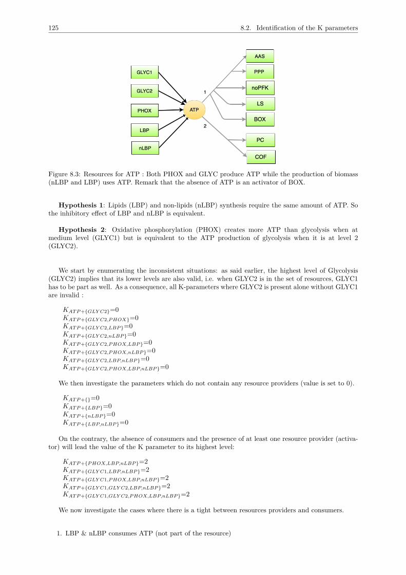
125 8.2. Identification of the K parameters
Figure 8.3: Resources for ATP : Both PHOX and GLYC produce ATP while the production of biomass(nLBP and LBP) uses ATP. Remark that the absence of ATP is an activator of BOX.
Hypothesis 1: Lipids (LBP) and non-lipids (nLBP) synthesis require the same amount of ATP. Sothe inhibitory effect of LBP and nLBP is equivalent.
Hypothesis 2: Oxidative phosphorylation (PHOX) creates more ATP than glycolysis when atmedium level (GLYC1) but is equivalent to the ATP production of glycolysis when it is at level 2(GLYC2).
We start by enumerating the inconsistent situations: as said earlier, the highest level of Glycolysis(GLYC2) implies that its lower levels are also valid, i.e. when GLYC2 is in the set of resources, GLYC1has to be part as well. As a consequence, all K-parameters where GLYC2 is present alone without GLYC1are invalid :
KAT P +{GLY C2}=0KAT P +{GLY C2,P HOX}=0KAT P +{GLY C2,LBP}=0KAT P +{GLY C2,nLBP}=0KAT P +{GLY C2,P HOX,LBP}=0KAT P +{GLY C2,P HOX,nLBP}=0KAT P +{GLY C2,LBP,nLBP}=0KAT P +{GLY C2,P HOX,LBP,nLBP}=0
We then investigate the parameters which do not contain any resource providers (value is set to 0).
KAT P +{}=0KAT P +{LBP}=0KAT P +{nLBP}=0KAT P +{LBP,nLBP}=0
On the contrary, the absence of consumers and the presence of at least one resource provider (activa-tor) will lead the value of the K parameter to its highest level:
KAT P +{P HOX,LBP,nLBP}=2KAT P +{GLY C1,LBP,nLBP}=2KAT P +{GLY C1,P HOX,LBP,nLBP}=2KAT P +{GLY C1,GLY C2,LBP,nLBP}=2KAT P +{GLY C1,GLY C2,P HOX,LBP,nLBP}=2
We now investigate the cases where there is a tight between resources providers and consumers.
1. LBP & nLBP consumes ATP (not part of the resource)
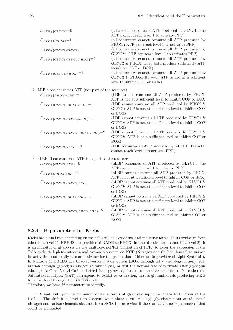
126 8.2. Identification of the K parameters
KAT P +{GLY C1}=0 (all consumers consume ATP produced by GLYC1 : theATP cannot reach level 1 to activate PPP)
KAT P +{P HOX}=1 (all consumers cannot consume all ATP produced byPHOX : ATP can reach level 1 to activates PPP)
KAT P +{GLY C1,GLY C2}=1 (all consumers cannot consume all ATP produced byGLYC2 : ATP can reach level 1 to activates PPP)
KAT P +{GLY C1,GLY C2,P HOX}=2 (all consumers cannot consume all ATP produced byGLYC2 & PHOX: They both produce sufficiently ATPto inhibit COF or BOX)
KAT P +{GLY C1,P HOX}=1 (all consumers cannot consume all ATP produced byGLYC2 & PHOX: However ATP is not at a sufficientlevel to inhibit COF or BOX)
2. LBP alone consumes ATP (not part of the resource)KAT P +{P HOX,nLBP}=1 (LBP cannot consume all ATP produced by PHOX:
ATP is not at a sufficient level to inhibit COF or BOXKAT P +{GLY C1,P HOX,nLBP}=1 (LBP cannot consume all ATP produced by PHOX &
GLYC1: ATP is not at a sufficient level to inhibit COFor BOX)
KAT P +{GLY C1,GLY C2,nLBP}=1 (LBP cannot consume all ATP produced by GLYC1 &GLYC2: ATP is not at a sufficient level to inhibit COFor BOX)
KAT P +{GLY C1,GLY C2,P HOX,nLBP}=2 (LBP cannot consume all ATP produced by GLYC1 &GLYC2: ATP is at a sufficient level to inhibit COF orBOX)
KAT P +{GLY C1,nLBP}=0 (LBP consumes all ATP produced by GLYC1 : the ATPcannot reach level 1 to activate PPP)
3. nLBP alone consumes ATP (not part of the resources)KAT P +{GLY C1,LBP}=0 (nLBP consumes all ATP produced by GLYC1 : the
ATP cannot reach level 1 to activate PPP)KAT P +{P HOX,LBP}=1 (nLBP cannot consume all ATP produced by PHOX:
ATP is not at a sufficient level to inhibit COF or BOX)KAT P +{GLY C1,GLY C2,LBP}=1 (nLBP cannot consume all ATP produced by GLYC1 &
GLYC2: ATP is not at a sufficient level to inhibit COFor BOX)
KAT P +{GLY C1,P HOX,LBP}=1 (nLBP cannot consume all ATP produced by PHOX &GLYC1: ATP is not at a sufficient level to inhibit COFor BOX)
KAT P +{GLY C1,GLY C2,P HOX,LBP}=2 (nLBP cannot consume all ATP produced by GLYC1 &GLYC2: ATP is at a sufficient level to inhibit COF orBOX)
8.2.4 K-parameters for KrebsKrebs has a dual role depending on the cell’s milieu : oxidative and reductive forms. In its oxidative form(that is at level 1), KREBS is a provider of NADH to PHOX. In its reductive form (that is at level 2), itis an inhibitor of glycolysis via the multiplex noPFK (inhibition of PFK) to lower the expression of theTCA cycle, it depletes nitrogen and carbon reservoirs via NCD (Nitrogen and Carbon donors) to sustainits activities, and finally it is an activator for the production of biomass (a provider of Lipid Synthesis).In Figure 8.4, KREBS has three resources : β-oxydation (BOX through fatty acid degradation), Sat-uration through (glycolysis and/or glutaminolysis) or just the normal fate of pyruvate after glycolysis(through AnO as Acetyl-CoA is derived from pyruvate, that is in normoxic condition). Note that theSaturation multiplex (SAT) correspond to oxidative saturation, that is glutaminolysis producing α-KGto be oxidized through the KREBS cycle.Therefore, we have 23 parameters to identify.
BOX and AnO provide minimum forces in terms of glycolytic input for Krebs to function at thelevel 1. The shift from level 1 to 2 occurs when there is either a high glycolytic input or additionalnitrogen and carbon elements obtained from NCD. Let us review if there are any kinetic parameters thatcould be eliminated.
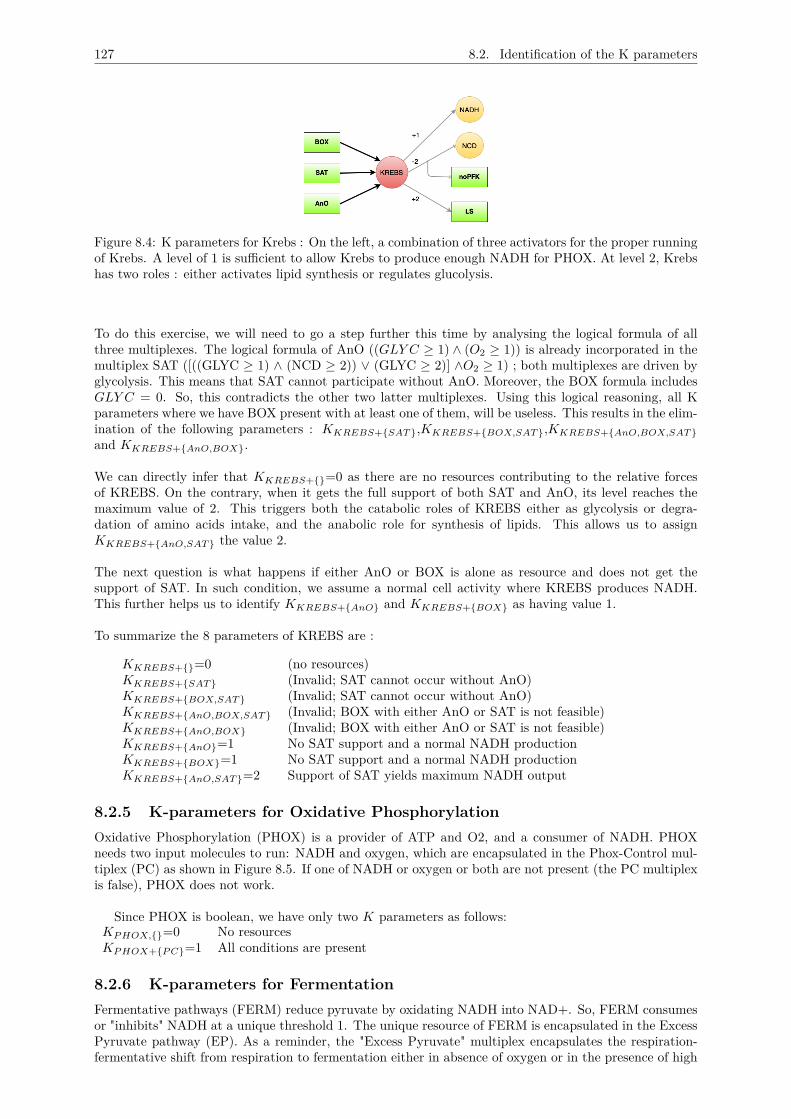
127 8.2. Identification of the K parameters
Figure 8.4: K parameters for Krebs : On the left, a combination of three activators for the proper runningof Krebs. A level of 1 is sufficient to allow Krebs to produce enough NADH for PHOX. At level 2, Krebshas two roles : either activates lipid synthesis or regulates glucolysis.
To do this exercise, we will need to go a step further this time by analysing the logical formula of allthree multiplexes. The logical formula of AnO ((GLY C ≥ 1) ∧ (O2 ≥ 1)) is already incorporated in themultiplex SAT ([((GLYC ≥ 1) ∧ (NCD ≥ 2)) ∨ (GLYC ≥ 2)] ∧O2 ≥ 1) ; both multiplexes are driven byglycolysis. This means that SAT cannot participate without AnO. Moreover, the BOX formula includesGLY C = 0. So, this contradicts the other two latter multiplexes. Using this logical reasoning, all Kparameters where we have BOX present with at least one of them, will be useless. This results in the elim-ination of the following parameters : KKREBS+{SAT},KKREBS+{BOX,SAT},KKREBS+{AnO,BOX,SAT}and KKREBS+{AnO,BOX}.
We can directly infer that KKREBS+{}=0 as there are no resources contributing to the relative forcesof KREBS. On the contrary, when it gets the full support of both SAT and AnO, its level reaches themaximum value of 2. This triggers both the catabolic roles of KREBS either as glycolysis or degra-dation of amino acids intake, and the anabolic role for synthesis of lipids. This allows us to assignKKREBS+{AnO,SAT} the value 2.
The next question is what happens if either AnO or BOX is alone as resource and does not get thesupport of SAT. In such condition, we assume a normal cell activity where KREBS produces NADH.This further helps us to identify KKREBS+{AnO} and KKREBS+{BOX} as having value 1.
To summarize the 8 parameters of KREBS are :
KKREBS+{}=0 (no resources)KKREBS+{SAT} (Invalid; SAT cannot occur without AnO)KKREBS+{BOX,SAT} (Invalid; SAT cannot occur without AnO)KKREBS+{AnO,BOX,SAT} (Invalid; BOX with either AnO or SAT is not feasible)KKREBS+{AnO,BOX} (Invalid; BOX with either AnO or SAT is not feasible)KKREBS+{AnO}=1 No SAT support and a normal NADH productionKKREBS+{BOX}=1 No SAT support and a normal NADH productionKKREBS+{AnO,SAT}=2 Support of SAT yields maximum NADH output
8.2.5 K-parameters for Oxidative PhosphorylationOxidative Phosphorylation (PHOX) is a provider of ATP and O2, and a consumer of NADH. PHOXneeds two input molecules to run: NADH and oxygen, which are encapsulated in the Phox-Control mul-tiplex (PC) as shown in Figure 8.5. If one of NADH or oxygen or both are not present (the PC multiplexis false), PHOX does not work.
Since PHOX is boolean, we have only two K parameters as follows:KP HOX,{}=0 No resourcesKP HOX+{P C}=1 All conditions are present
8.2.6 K-parameters for FermentationFermentative pathways (FERM) reduce pyruvate by oxidating NADH into NAD+. So, FERM consumesor "inhibits" NADH at a unique threshold 1. The unique resource of FERM is encapsulated in the ExcessPyruvate pathway (EP). As a reminder, the "Excess Pyruvate" multiplex encapsulates the respiration-fermentative shift from respiration to fermentation either in absence of oxygen or in the presence of high
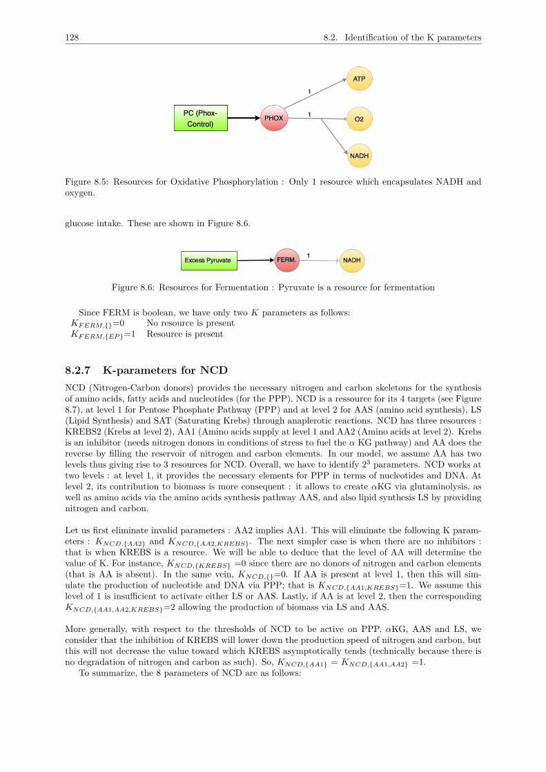
128 8.2. Identification of the K parameters
Figure 8.5: Resources for Oxidative Phosphorylation : Only 1 resource which encapsulates NADH andoxygen.
glucose intake. These are shown in Figure 8.6.
Figure 8.6: Resources for Fermentation : Pyruvate is a resource for fermentation
Since FERM is boolean, we have only two K parameters as follows:KF ERM,{}=0 No resource is presentKF ERM,{EP}=1 Resource is present
8.2.7 K-parameters for NCDNCD (Nitrogen-Carbon donors) provides the necessary nitrogen and carbon skeletons for the synthesisof amino acids, fatty acids and nucleotides (for the PPP). NCD is a ressource for its 4 targets (see Figure8.7), at level 1 for Pentose Phosphate Pathway (PPP) and at level 2 for AAS (amino acid synthesis), LS(Lipid Synthesis) and SAT (Saturating Krebs) through anaplerotic reactions. NCD has three resources :KREBS2 (Krebs at level 2), AA1 (Amino acids supply at level 1 and AA2 (Amino acids at level 2). Krebsis an inhibitor (needs nitrogen donors in conditions of stress to fuel the α KG pathway) and AA does thereverse by filling the reservoir of nitrogen and carbon elements. In our model, we assume AA has twolevels thus giving rise to 3 resources for NCD. Overall, we have to identify 23 parameters. NCD works attwo levels : at level 1, it provides the necessary elements for PPP in terms of nucleotides and DNA. Atlevel 2, its contribution to biomass is more consequent : it allows to create αKG via glutaminolysis, aswell as amino acids via the amino acids synthesis pathway AAS, and also lipid synthesis LS by providingnitrogen and carbon.
Let us first eliminate invalid parameters : AA2 implies AA1. This will eliminate the following K param-eters : KNCD,{AA2} and KNCD,{AA2,KREBS}. The next simpler case is when there are no inhibitors :that is when KREBS is a resource. We will be able to deduce that the level of AA will determine thevalue of K. For instance, KNCD,{KREBS} =0 since there are no donors of nitrogen and carbon elements(that is AA is absent). In the same vein, KNCD,{}=0. If AA is present at level 1, then this will sim-ulate the production of nucleotide and DNA via PPP; that is KNCD,{AA1,KREBS}=1. We assume thislevel of 1 is insufficient to activate either LS or AAS. Lastly, if AA is at level 2, then the correspondingKNCD,{AA1,AA2,KREBS}=2 allowing the production of biomass via LS and AAS.
More generally, with respect to the thresholds of NCD to be active on PPP, αKG, AAS and LS, weconsider that the inhibition of KREBS will lower down the production speed of nitrogen and carbon, butthis will not decrease the value toward which KREBS asymptotically tends (technically because there isno degradation of nitrogen and carbon as such). So, KNCD,{AA1} = KNCD,{AA1,AA2} =1.
To summarize, the 8 parameters of NCD are as follows:
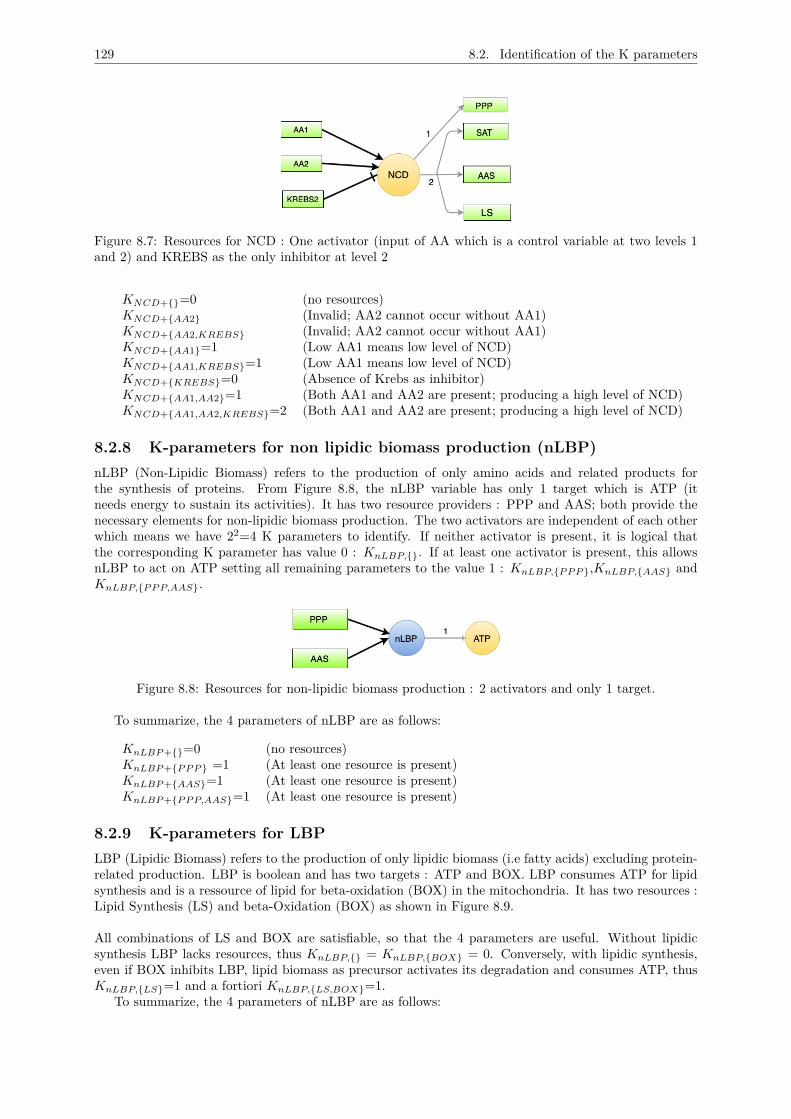
129 8.2. Identification of the K parameters
Figure 8.7: Resources for NCD : One activator (input of AA which is a control variable at two levels 1and 2) and KREBS as the only inhibitor at level 2
KNCD+{}=0 (no resources)KNCD+{AA2} (Invalid; AA2 cannot occur without AA1)KNCD+{AA2,KREBS} (Invalid; AA2 cannot occur without AA1)KNCD+{AA1}=1 (Low AA1 means low level of NCD)KNCD+{AA1,KREBS}=1 (Low AA1 means low level of NCD)KNCD+{KREBS}=0 (Absence of Krebs as inhibitor)KNCD+{AA1,AA2}=1 (Both AA1 and AA2 are present; producing a high level of NCD)KNCD+{AA1,AA2,KREBS}=2 (Both AA1 and AA2 are present; producing a high level of NCD)
8.2.8 K-parameters for non lipidic biomass production (nLBP)nLBP (Non-Lipidic Biomass) refers to the production of only amino acids and related products forthe synthesis of proteins. From Figure 8.8, the nLBP variable has only 1 target which is ATP (itneeds energy to sustain its activities). It has two resource providers : PPP and AAS; both provide thenecessary elements for non-lipidic biomass production. The two activators are independent of each otherwhich means we have 22=4 K parameters to identify. If neither activator is present, it is logical thatthe corresponding K parameter has value 0 : KnLBP,{}. If at least one activator is present, this allowsnLBP to act on ATP setting all remaining parameters to the value 1 : KnLBP,{P P P},KnLBP,{AAS} andKnLBP,{P P P,AAS}.
Figure 8.8: Resources for non-lipidic biomass production : 2 activators and only 1 target.
To summarize, the 4 parameters of nLBP are as follows:
KnLBP +{}=0 (no resources)KnLBP +{P P P} =1 (At least one resource is present)KnLBP +{AAS}=1 (At least one resource is present)KnLBP +{P P P,AAS}=1 (At least one resource is present)
8.2.9 K-parameters for LBPLBP (Lipidic Biomass) refers to the production of only lipidic biomass (i.e fatty acids) excluding protein-related production. LBP is boolean and has two targets : ATP and BOX. LBP consumes ATP for lipidsynthesis and is a ressource of lipid for beta-oxidation (BOX) in the mitochondria. It has two resources :Lipid Synthesis (LS) and beta-Oxidation (BOX) as shown in Figure 8.9.
All combinations of LS and BOX are satisfiable, so that the 4 parameters are useful. Without lipidicsynthesis LBP lacks resources, thus KnLBP,{} = KnLBP,{BOX} = 0. Conversely, with lipidic synthesis,even if BOX inhibits LBP, lipid biomass as precursor activates its degradation and consumes ATP, thusKnLBP,{LS}=1 and a fortiori KnLBP,{LS,BOX}=1.
To summarize, the 4 parameters of nLBP are as follows:
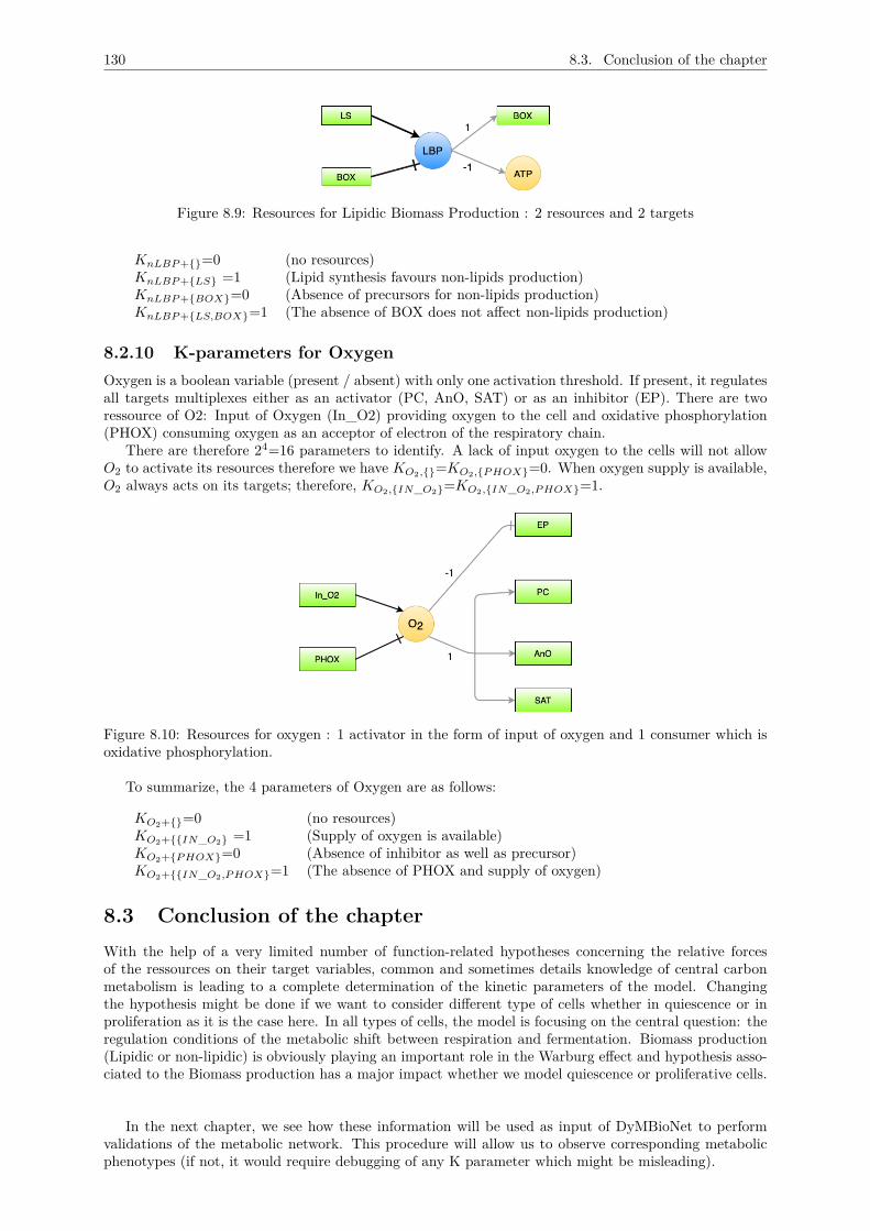
130 8.3. Conclusion of the chapter
Figure 8.9: Resources for Lipidic Biomass Production : 2 resources and 2 targets
KnLBP +{}=0 (no resources)KnLBP +{LS} =1 (Lipid synthesis favours non-lipids production)KnLBP +{BOX}=0 (Absence of precursors for non-lipids production)KnLBP +{LS,BOX}=1 (The absence of BOX does not affect non-lipids production)
8.2.10 K-parameters for OxygenOxygen is a boolean variable (present / absent) with only one activation threshold. If present, it regulatesall targets multiplexes either as an activator (PC, AnO, SAT) or as an inhibitor (EP). There are tworessource of O2: Input of Oxygen (In_O2) providing oxygen to the cell and oxidative phosphorylation(PHOX) consuming oxygen as an acceptor of electron of the respiratory chain.
There are therefore 24=16 parameters to identify. A lack of input oxygen to the cells will not allowO2 to activate its resources therefore we have KO2,{}=KO2,{P HOX}=0. When oxygen supply is available,O2 always acts on its targets; therefore, KO2,{IN_O2}=KO2,{IN_O2,P HOX}=1.
Figure 8.10: Resources for oxygen : 1 activator in the form of input of oxygen and 1 consumer which isoxidative phosphorylation.
To summarize, the 4 parameters of Oxygen are as follows:
KO2+{}=0 (no resources)KO2+{{IN_O2} =1 (Supply of oxygen is available)KO2+{P HOX}=0 (Absence of inhibitor as well as precursor)KO2+{{IN_O2,P HOX}=1 (The absence of PHOX and supply of oxygen)
8.3 Conclusion of the chapterWith the help of a very limited number of function-related hypotheses concerning the relative forcesof the ressources on their target variables, common and sometimes details knowledge of central carbonmetabolism is leading to a complete determination of the kinetic parameters of the model. Changingthe hypothesis might be done if we want to consider different type of cells whether in quiescence or inproliferation as it is the case here. In all types of cells, the model is focusing on the central question: theregulation conditions of the metabolic shift between respiration and fermentation. Biomass production(Lipidic or non-lipidic) is obviously playing an important role in the Warburg effect and hypothesis asso-ciated to the Biomass production has a major impact whether we model quiescence or proliferative cells.
In the next chapter, we see how these information will be used as input of DyMBioNet to performvalidations of the metabolic network. This procedure will allow us to observe corresponding metabolicphenotypes (if not, it would require debugging of any K parameter which might be misleading).
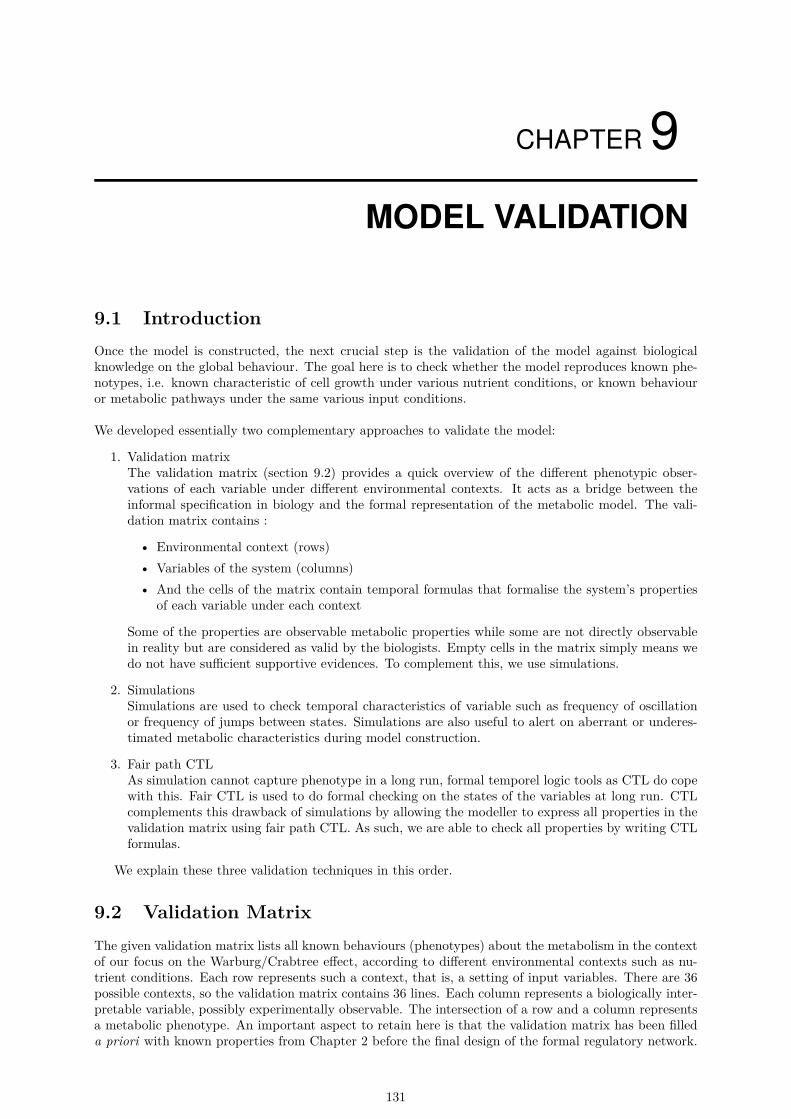
CHAPTER 9MODEL VALIDATION
9.1 IntroductionOnce the model is constructed, the next crucial step is the validation of the model against biologicalknowledge on the global behaviour. The goal here is to check whether the model reproduces known phe-notypes, i.e. known characteristic of cell growth under various nutrient conditions, or known behaviouror metabolic pathways under the same various input conditions.
We developed essentially two complementary approaches to validate the model:
1. Validation matrixThe validation matrix (section 9.2) provides a quick overview of the different phenotypic obser-vations of each variable under different environmental contexts. It acts as a bridge between theinformal specification in biology and the formal representation of the metabolic model. The vali-dation matrix contains :
• Environmental context (rows)• Variables of the system (columns)• And the cells of the matrix contain temporal formulas that formalise the system’s properties
of each variable under each context
Some of the properties are observable metabolic properties while some are not directly observablein reality but are considered as valid by the biologists. Empty cells in the matrix simply means wedo not have sufficient supportive evidences. To complement this, we use simulations.
2. SimulationsSimulations are used to check temporal characteristics of variable such as frequency of oscillationor frequency of jumps between states. Simulations are also useful to alert on aberrant or underes-timated metabolic characteristics during model construction.
3. Fair path CTLAs simulation cannot capture phenotype in a long run, formal temporel logic tools as CTL do copewith this. Fair CTL is used to do formal checking on the states of the variables at long run. CTLcomplements this drawback of simulations by allowing the modeller to express all properties in thevalidation matrix using fair path CTL. As such, we are able to check all properties by writing CTLformulas.
We explain these three validation techniques in this order.
9.2 Validation MatrixThe given validation matrix lists all known behaviours (phenotypes) about the metabolism in the contextof our focus on the Warburg/Crabtree effect, according to different environmental contexts such as nu-trient conditions. Each row represents such a context, that is, a setting of input variables. There are 36possible contexts, so the validation matrix contains 36 lines. Each column represents a biologically inter-pretable variable, possibly experimentally observable. The intersection of a row and a column representsa metabolic phenotype. An important aspect to retain here is that the validation matrix has been filleda priori with known properties from Chapter 2 before the final design of the formal regulatory network.
131
132 9.2. Validation Matrix
There are 4 input variables (FA, in_O2, GLC and AA) which describe the environmental contextfor our metabolic model and 10 variables of the system which describe metabolic processes. Note thatthe asymptotic behaviour of variable NCD depends directly of the variable AA, consequently the NCDcolumn would be a copy (up to the ”tend()” pattern) to the AA column and therefore is omitted fromthe validation matrix. Among the input variables, in_O2 and FA are boolean while AA and GLC havethree values (boundary=2). This gives us 36 possibilities (2 x 2 x 3 x 3), which gives rise to 36 rows inthe validation matrix : 36 possible biological contexts.
As there are 9 variables, there is a total of 9 x 36 behaviours for all 9 variables whether they oscillateor tend to a stationary state. These two global behaviours of the variable can be coded in term of FairCTL formula and it is therefore possible to determine whether each variable oscillate or not under the36 input environmental conditions. There are potentially 9x36 Fair CTL formula constructed for thisvalidation matrix, but some are gray box as already mentioned(see Table 9.1).
The "oscillatory" or "tend towards" behaviour are encoded as follows:
1. tend represented by "tendTowards" function which accepts two parameters : a variable and theinteger value towards which the variable should go.Using Fair CTL, tend(n) for a variable x is simply encoded as AF (AG(x = n). Notice that, con-trarily to CTL, the A quantifier does not take into account unfair paths where a possible transitionfrom a given state is ignored while this state is visited an infinite number of times.
2. osc meaning an alternance between two extreme values represented by the "oscillate" function. Thisfunction accepts the variable three parameters : the variable and the two extreme values betweenwhich the variable will oscillate.osc(m,n) for a variable x is encoded as follows in Fair CTL : AF (x = m) ∧ AF (x = n) and weadopt a model checking strategy such that we retain the smallest possible value m and the highestpossible value n in the model.
Moreover, in Table 9.1, "!" stands for negation. Each test is detailed in the order they appear inthe validation matrix of Table 9.1. We regroup the 36 biological contexts into 4 categories defining theboolean combination of lipids and oxygen supply (first 2 columns of the matrix). In some cases, whenthe phenotypes resemble, we combine the biological context (rows 2 & 3 for example). When no generalknowledge about the behaviour of a given variable in a given context is available, the corresponding boxremains empty (dark grey). We will try to answer these missing information later on using simulationsand CTL.
9.2.1 No lipids and oxygen supply : FA=0 & In_O2 = 0We explain rows 1 - 8 with different combinations of glucose and amino acids. If there is no supply ofoxygen, it is feasible enough to say that oxygen (O2) will tend to 0 and PHOX also will tend to 0 as itis highly dependent on oxygen.
• ROW 1 : GLC= 0, AA = 0Cells fail to receive the necessary nutrient for growth and even survive : each variable should tendto zero.
• ROW 2 & 3 : GLC=0, AA = 1, 2Without glucose, cells can survive if the carbon source is represented by amino acids. (There areindeed nutritive milieu without glucose for certain cancer cell lines [157, 158]). Cell energy (ATP) isproduced through cataplerotic feeding of amino acids to KREBS cycle which works as an oxidativemachinery connected to PHOX to produce ATP. So without O2, the oxidative process is not possibleand all non-gray variables (i.e. O2) tend to 0.
• ROW 4 : GLC = 1 and AA = 0In the absence of oxygen, cells use glucose to ferment due to the delta redox reactions of NADH. Alow glucose is sufficient to allow the production of lactate which reduces NADH to NAD+, which isrecycled back to glycolysis (NADH will therefore oscillate). Mitochondrial activity is shunted andcytosolic metabolism of glucose follows the unidirectional transformation of glucose molecules topyruvate and finally to lactate. Following these explanations, we expect the following phenotypicobservations: at least fermentation is not down, Krebs and PHOX must maintain a low state,other related cofactors in this glycolysis-fermentation cycle will manifest with time. So, GLYC will
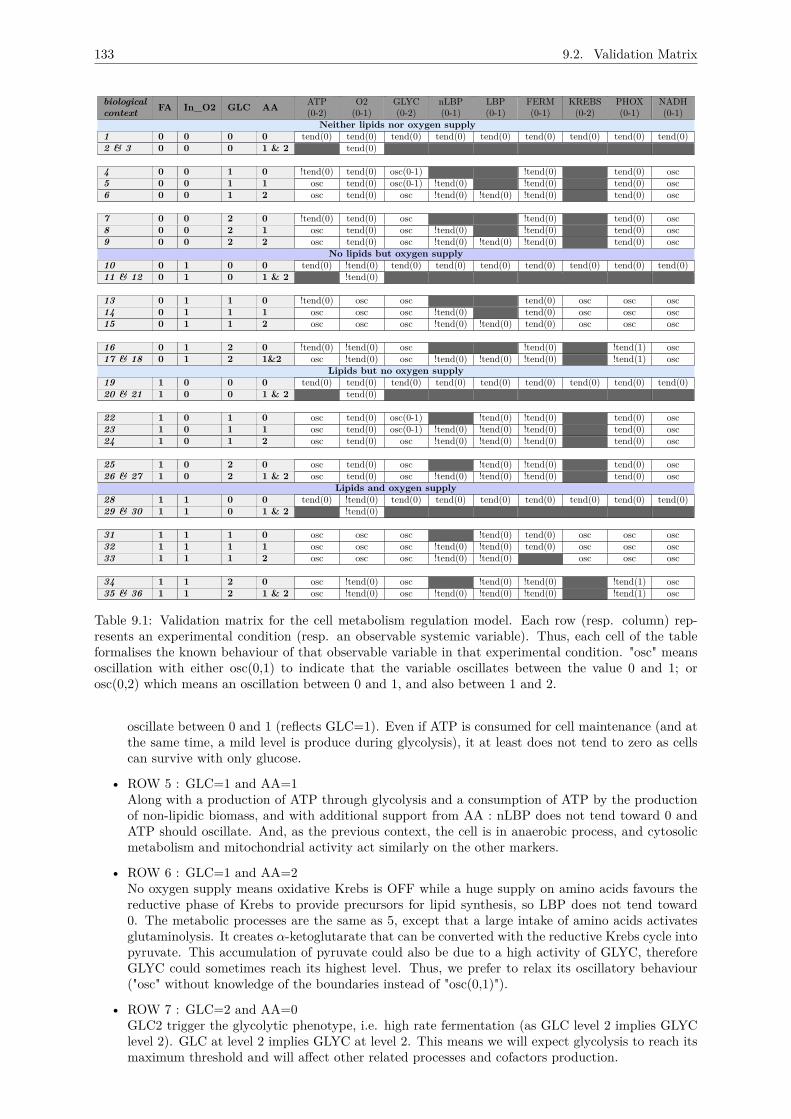
133 9.2. Validation Matrix
biologicalcontext FA In_O2 GLC AA ATP
(0-2)O2(0-1)
GLYC(0-2)
nLBP(0-1)
LBP(0-1)
FERM(0-1)
KREBS(0-2)
PHOX(0-1)
NADH(0-1)
Neither lipids nor oxygen supply1 0 0 0 0 tend(0) tend(0) tend(0) tend(0) tend(0) tend(0) tend(0) tend(0) tend(0)2 & 3 0 0 0 1 & 2 tend(0)
4 0 0 1 0 !tend(0) tend(0) osc(0-1) !tend(0) tend(0) osc5 0 0 1 1 osc tend(0) osc(0-1) !tend(0) !tend(0) tend(0) osc6 0 0 1 2 osc tend(0) osc !tend(0) !tend(0) !tend(0) tend(0) osc
7 0 0 2 0 !tend(0) tend(0) osc !tend(0) tend(0) osc8 0 0 2 1 osc tend(0) osc !tend(0) !tend(0) tend(0) osc9 0 0 2 2 osc tend(0) osc !tend(0) !tend(0) !tend(0) tend(0) osc
No lipids but oxygen supply10 0 1 0 0 tend(0) !tend(0) tend(0) tend(0) tend(0) tend(0) tend(0) tend(0) tend(0)11 & 12 0 1 0 1 & 2 !tend(0)
13 0 1 1 0 !tend(0) osc osc tend(0) osc osc osc14 0 1 1 1 osc osc osc !tend(0) tend(0) osc osc osc15 0 1 1 2 osc osc osc !tend(0) !tend(0) tend(0) osc osc osc
16 0 1 2 0 !tend(0) !tend(0) osc !tend(0) !tend(1) osc17 & 18 0 1 2 1&2 osc !tend(0) osc !tend(0) !tend(0) !tend(0) !tend(1) osc
Lipids but no oxygen supply19 1 0 0 0 tend(0) tend(0) tend(0) tend(0) tend(0) tend(0) tend(0) tend(0) tend(0)20 & 21 1 0 0 1 & 2 tend(0)
22 1 0 1 0 osc tend(0) osc(0-1) !tend(0) !tend(0) tend(0) osc23 1 0 1 1 osc tend(0) osc(0-1) !tend(0) !tend(0) !tend(0) tend(0) osc24 1 0 1 2 osc tend(0) osc !tend(0) !tend(0) !tend(0) tend(0) osc
25 1 0 2 0 osc tend(0) osc !tend(0) !tend(0) tend(0) osc26 & 27 1 0 2 1 & 2 osc tend(0) osc !tend(0) !tend(0) !tend(0) tend(0) osc
Lipids and oxygen supply28 1 1 0 0 tend(0) !tend(0) tend(0) tend(0) tend(0) tend(0) tend(0) tend(0) tend(0)29 & 30 1 1 0 1 & 2 !tend(0)
31 1 1 1 0 osc osc osc !tend(0) tend(0) osc osc osc32 1 1 1 1 osc osc osc !tend(0) !tend(0) tend(0) osc osc osc33 1 1 1 2 osc osc osc !tend(0) !tend(0) osc osc osc
34 1 1 2 0 osc !tend(0) osc !tend(0) !tend(0) !tend(1) osc35 & 36 1 1 2 1 & 2 osc !tend(0) osc !tend(0) !tend(0) !tend(0) !tend(1) osc
Table 9.1: Validation matrix for the cell metabolism regulation model. Each row (resp. column) rep-resents an experimental condition (resp. an observable systemic variable). Thus, each cell of the tableformalises the known behaviour of that observable variable in that experimental condition. "osc" meansoscillation with either osc(0,1) to indicate that the variable oscillates between the value 0 and 1; orosc(0,2) which means an oscillation between 0 and 1, and also between 1 and 2.
oscillate between 0 and 1 (reflects GLC=1). Even if ATP is consumed for cell maintenance (and atthe same time, a mild level is produce during glycolysis), it at least does not tend to zero as cellscan survive with only glucose.
• ROW 5 : GLC=1 and AA=1Along with a production of ATP through glycolysis and a consumption of ATP by the productionof non-lipidic biomass, and with additional support from AA : nLBP does not tend toward 0 andATP should oscillate. And, as the previous context, the cell is in anaerobic process, and cytosolicmetabolism and mitochondrial activity act similarly on the other markers.
• ROW 6 : GLC=1 and AA=2No oxygen supply means oxidative Krebs is OFF while a huge supply on amino acids favours thereductive phase of Krebs to provide precursors for lipid synthesis, so LBP does not tend toward0. The metabolic processes are the same as 5, except that a large intake of amino acids activatesglutaminolysis. It creates α-ketoglutarate that can be converted with the reductive Krebs cycle intopyruvate. This accumulation of pyruvate could also be due to a high activity of GLYC, thereforeGLYC could sometimes reach its highest level. Thus, we prefer to relax its oscillatory behaviour("osc" without knowledge of the boundaries instead of "osc(0,1)").
• ROW 7 : GLC=2 and AA=0GLC2 trigger the glycolytic phenotype, i.e. high rate fermentation (as GLC level 2 implies GLYClevel 2). GLC at level 2 implies GLYC at level 2. This means we will expect glycolysis to reach itsmaximum threshold and will affect other related processes and cofactors production.
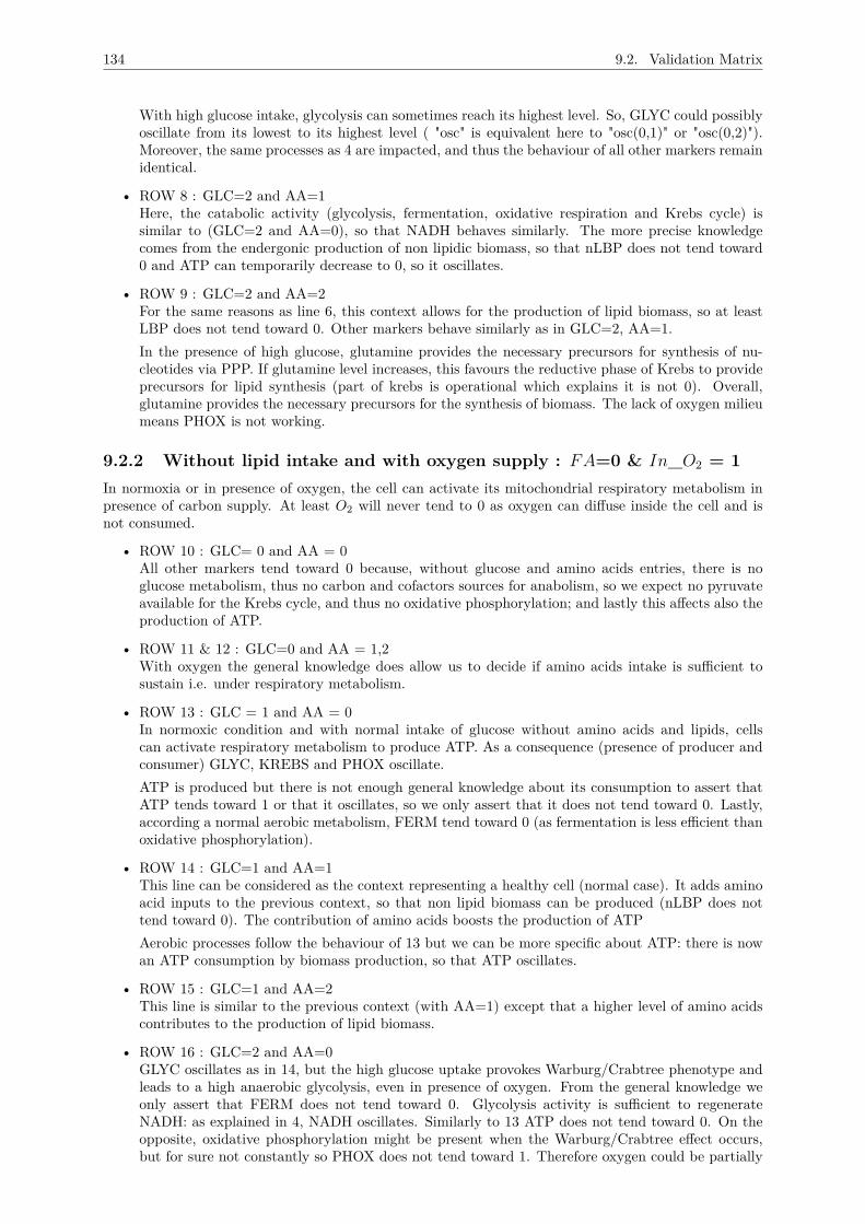
134 9.2. Validation Matrix
With high glucose intake, glycolysis can sometimes reach its highest level. So, GLYC could possiblyoscillate from its lowest to its highest level ( "osc" is equivalent here to "osc(0,1)" or "osc(0,2)").Moreover, the same processes as 4 are impacted, and thus the behaviour of all other markers remainidentical.
• ROW 8 : GLC=2 and AA=1Here, the catabolic activity (glycolysis, fermentation, oxidative respiration and Krebs cycle) issimilar to (GLC=2 and AA=0), so that NADH behaves similarly. The more precise knowledgecomes from the endergonic production of non lipidic biomass, so that nLBP does not tend toward0 and ATP can temporarily decrease to 0, so it oscillates.
• ROW 9 : GLC=2 and AA=2For the same reasons as line 6, this context allows for the production of lipid biomass, so at leastLBP does not tend toward 0. Other markers behave similarly as in GLC=2, AA=1.In the presence of high glucose, glutamine provides the necessary precursors for synthesis of nu-cleotides via PPP. If glutamine level increases, this favours the reductive phase of Krebs to provideprecursors for lipid synthesis (part of krebs is operational which explains it is not 0). Overall,glutamine provides the necessary precursors for the synthesis of biomass. The lack of oxygen milieumeans PHOX is not working.
9.2.2 Without lipid intake and with oxygen supply : FA=0 & In_O2 = 1In normoxia or in presence of oxygen, the cell can activate its mitochondrial respiratory metabolism inpresence of carbon supply. At least O2 will never tend to 0 as oxygen can diffuse inside the cell and isnot consumed.
• ROW 10 : GLC= 0 and AA = 0All other markers tend toward 0 because, without glucose and amino acids entries, there is noglucose metabolism, thus no carbon and cofactors sources for anabolism, so we expect no pyruvateavailable for the Krebs cycle, and thus no oxidative phosphorylation; and lastly this affects also theproduction of ATP.
• ROW 11 & 12 : GLC=0 and AA = 1,2With oxygen the general knowledge does allow us to decide if amino acids intake is sufficient tosustain i.e. under respiratory metabolism.
• ROW 13 : GLC = 1 and AA = 0In normoxic condition and with normal intake of glucose without amino acids and lipids, cellscan activate respiratory metabolism to produce ATP. As a consequence (presence of producer andconsumer) GLYC, KREBS and PHOX oscillate.ATP is produced but there is not enough general knowledge about its consumption to assert thatATP tends toward 1 or that it oscillates, so we only assert that it does not tend toward 0. Lastly,according a normal aerobic metabolism, FERM tend toward 0 (as fermentation is less efficient thanoxidative phosphorylation).
• ROW 14 : GLC=1 and AA=1This line can be considered as the context representing a healthy cell (normal case). It adds aminoacid inputs to the previous context, so that non lipid biomass can be produced (nLBP does nottend toward 0). The contribution of amino acids boosts the production of ATPAerobic processes follow the behaviour of 13 but we can be more specific about ATP: there is nowan ATP consumption by biomass production, so that ATP oscillates.
• ROW 15 : GLC=1 and AA=2This line is similar to the previous context (with AA=1) except that a higher level of amino acidscontributes to the production of lipid biomass.
• ROW 16 : GLC=2 and AA=0GLYC oscillates as in 14, but the high glucose uptake provokes Warburg/Crabtree phenotype andleads to a high anaerobic glycolysis, even in presence of oxygen. From the general knowledge weonly assert that FERM does not tend toward 0. Glycolysis activity is sufficient to regenerateNADH: as explained in 4, NADH oscillates. Similarly to 13 ATP does not tend toward 0. On theopposite, oxidative phosphorylation might be present when the Warburg/Crabtree effect occurs,but for sure not constantly so PHOX does not tend toward 1. Therefore oxygen could be partially
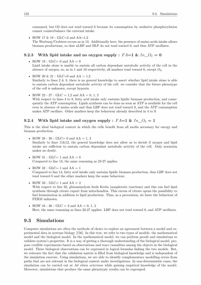
135 9.3. Simulations
consumed, but O2 does not tend toward 0 because its consumption by oxidative phosphorylationcannot counterbalance the external intake.
• ROW 17 & 18 : GLC=2 and AA=1,2The Warburg/Crabtree occurs as in 13. Additionally here, the presence of amino acids intake allowsbiomass productions, so that nLBP and BLP do not tend toward 0, and thus ATP oscillates.
9.2.3 With lipid intake and no oxygen supply : FA=1 & In_O2 = 0• ROW 19 : GLC= 0 and AA = 0
Lipid intake alone is unable to sustain all carbon dependant metabolic activity of the cell in theabsence of oxygen, so, as in 1 and 10 respectively, all markers tend toward 0, except O2.
• ROW 20 & 21 : GLC=0 and AA = 1,2Similarly to lines 2 & 3, there is no general knowledge to assert whether lipid intake alone is ableto sustain carbon dependant metabolic activity of the cell: we consider that the future phenotypeof the cell is unknown, except hypoxia.
• ROW 22 - 27 : GLC = 1,2 and AA = 0, 1, 2With respect to lines 4 to 9, fatty acid intake only sustains lipidic biomass production, and conse-quently the ATP consumption. Lipids synthesis can be done as soon as ATP is available for the celleven in absence of amino acids and thus LBP does not tend toward 0, and the ATP consumptionmakes ATP oscillate. Other markers keep the behaviour already described in 4 to 9.
9.2.4 With lipid intake and oxygen supply : FA=1 & In_O2 = 1This is the ideal biological context in which the cells benefit from all media necessary for energy andbiomass production.
• ROW 28 - 30 : GLC= 0 and AA = 1, 2Similarly to lines 11&12, the general knowledge does not allow us to decide if oxygen and lipidintake are sufficient to sustain carbon dependant metabolic activity of the cell. Only normoxiamakes no doubt.
• ROW 31 : GLC= 1 and AA = 0Compared to line 13, the same reasoning as 22-27 applies.
• ROW 32 : GLC= 1 and AA = 1Compared to line 14, fatty acid intake only sustains lipidic biomass production, thus LBP does nottend toward 0 and the other markers keep the same behaviour.
• ROW 33 : GLC= 1 and AA = 2With respect to line 32, glutaminolysis feeds Krebs (anaplerotic reactions) and this can fuel lipidsynthesis through citrate export from mitochondria. This excess of citrate opens the possibility tofuel fermentation in addition to lipid production. Thus, as a precaution, we leave the behaviour ofFERM unknown.
• ROW 34 - 36 : GLC = 2 and AA = 0, 1, 2Here, the same reasoning as lines 22-27 applies: LBP does not tend toward 0, and ATP oscillates.
9.3 SimulationsComputer simulations are often the methods of choice to explore an agreement between a model and ex-perimental data in systems biology [156]. In this text, we refer to two types of models: the mathematicalmodel and the biological model. In the mathematical model, we can perform proofs and simulations tovalidate system’s properties. It is a way of getting a thorough understanding of the biological model, pro-pose credible experiments based on observations and trace causalities among the objects in the biologicalmodel. These biological observations can be expressed in logical formulas linking the two models. But,we reiterate the fact that the validation matrix is filled from biological knowledge and is independent ofthe simulation exercise. Using simulations, we are able to identify complementary modelling errors frompaths that are not relevant in the biological context under investigations. In non-deterministic cases, thesimulation can be carried out at Ad vitam aeternam while gaining empirical knowledge of the model.Moreover, simulations that produce the same phenotypic results can be regrouped.
136 9.3. Simulations
In this section, we will perform simulations to demonstrate three well-known phenotypic characteris-tics of metabolism : respiration, fermentation, and the CrabTree effect in fermenting yeast. In thesethree different phenotypes, we will have the chance to see how simulations are helpful and how we canalso mimic the cellular environment based on availability of nutrients.
9.3.1 Environmental context of Row 13 : FA=0 & In_O2 = 1, GLC = 1 andAA = 0
As a reminder, respiration takes place when cells have sufficient amount of oxygen to degrade glucose,and Krebs and PHOX are functioning normally. During this respiration process, the ultimate goal of thecells is to provide sufficient energy for maintenance and growth. As a result of this glucose metabolism,the following key oscillations occur in the cells and for simplicity, we put the curve colour within bracketas shown in Figure 9.1.
• NADH/NAD+ (grenat)Oscillation of NADH/NAD+ occurs as NAD+ is reduced to NADH during glycolysis and in themitochondria, NADH is oxidised back to NAD+. So, overall, the concentration of NADH/NAD+needs to remain homeostatic which justifies this oscillatory behaviour.
• ATP/ADP (red)The production of ATP is mostly likely to increase as soon as the mitochondria activity starts: thisis visible in the graph as KREBS and PHOX becomes active, that is they switch from 0 to 1. ATPalso changes from a threshold of 0 to 1, then slowly from 1 to 2.
• GLYC (yellow)Assuming a constant supply of glucose, the process of glycolysis oscillates as it consumes NAD+to produce NADH and recovers it back from the mitochondria. This balance of NADH/NAD+ ismaintained by glycolysis and Krebs in normoxic conditions. This shows the existence of a certainkind of feedback control which is important to catalyse intermediate reactions.
• KREBS (black)Krebs also is likely to fluctuate depending on the availability of its input sources: mostly pyruvateand in condition of stress, acetyl CoA from degradation of fatty acids. When glycolysis oscillates,KREBS also will oscillate as it is dependent on the end products of glycolysis.
• PHOX (green)The dependency of oxidative phosphorylation on Krebs for cofactors NADH and FADH accountsfor its fluctuations and this dependency is visible in the graph; PHOX appears after KREBS withtime.
9.3.2 Environmental context of Row 18 : FA=0 & In_O2 = 1, GLC=2 andAA=2
This is the case of normal respiration where we have excess of both amino acids and glucose. Excessof glucose can favours the fermentation process even in the presence of oxygen (FERM oscillates in thegraph 9.2). Similarly, these variables do not tend to 0 but rather oscillate: GLYC, ATP, NADH andNCD.
9.3.3 Environmental context of Row 20 & 21 : FA=0 & In_O2 = 1, GLC=0and AA = 1,2
The prime nutrients (glucose and oxygen) are absent. Fatty acids and amino acids are the only nutrientsfor the cells, which contribute to the nitrogen and carbon elements for future use. From Figure 9.3,stable state is reached both in the case of Row 20 & 21. This means that all variables will maintain theiroriginal values and will not change in such conditions.
9.3.4 Environmental context of Row 29 : FA=1 & In_O2 = 1, GLC=0 andAA = 1
Similar to the previous cases, here also stable state is reached quickly. From Figure 9.4, we can see thatboth O2 and NCD tend to 1. Other variables will normally stay at their assigned values.
137 9.3. Simulations
Figure 9.1: Normal Respiration with only input of glucose and oxygen.
Figure 9.2: Respiration with normal glucose and excess amino acids
9.3.5 Environmental context of Row 35 : FA=1 & In_O2 = 1, GLC=2 andAA = 1
From Figure 9.5, we can see that the majority of the variables will have the tendency to change from thevalue 0 to another value. In these conditions, the status of the KREBS shift from 0 and oscillates. Thisallows us to complete the missing interpretation at row 35 in the validation matrix.
Many biological systems exhibit non-deterministic behaviour. When simulating a dynamical model,it may happen (as it is the case more often) that certain trajectories appear after a very long timedue to the non-deterministic behaviour and randomness of certain primary components of the system.Contrarily, it may also happen that some unexpected properties are observed during simulations but thisdoes not readily means that we have refuted the model. Again, due to this non-deterministic feature,some trajectories have less probability of being chosen and their turn may happen after a long time.
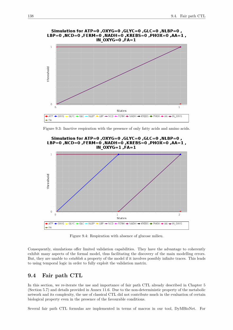
138 9.4. Fair path CTL
Figure 9.3: Inactive respiration with the presence of only fatty acids and amino acids.
Figure 9.4: Respiration with absence of glucose milieu.
Consequently, simulations offer limited validation capabilities. They have the advantage to coherentlyexhibit many aspects of the formal model, thus facilitating the discovery of the main modelling errors.But, they are unable to establish a property of the model if it involves possibly infinite traces. This leadsto using temporal logic in order to fully exploit the validation matrix.
9.4 Fair path CTLIn this section, we re-iterate the use and importance of fair path CTL already described in Chapter 5(Section 5.7) and details provided in Annex 11.6. Due to the non-deterministic property of the metabolicnetwork and its complexity, the use of classical CTL did not contribute much in the evaluation of certainbiological property even in the presence of the favourable conditions.
Several fair path CTL formulas are implemented in terms of macros in our tool, DyMBioNet. For
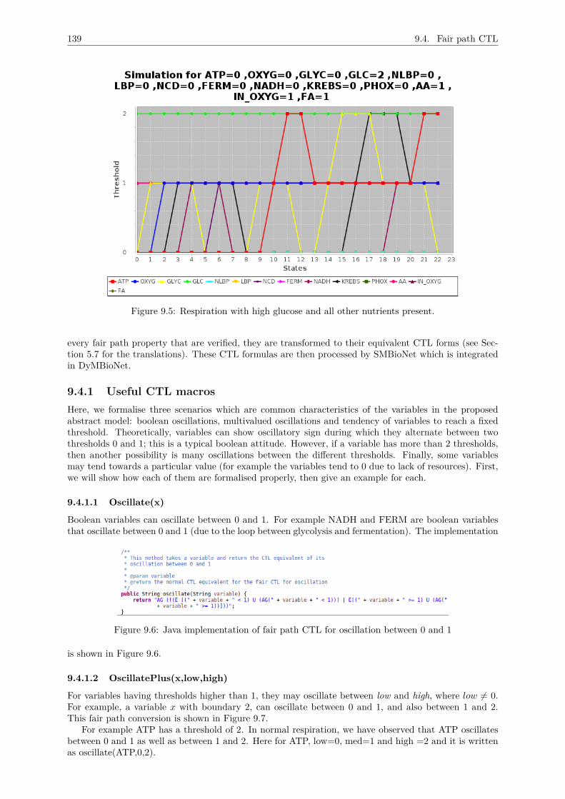
139 9.4. Fair path CTL
Figure 9.5: Respiration with high glucose and all other nutrients present.
every fair path property that are verified, they are transformed to their equivalent CTL forms (see Sec-tion 5.7 for the translations). These CTL formulas are then processed by SMBioNet which is integratedin DyMBioNet.
9.4.1 Useful CTL macrosHere, we formalise three scenarios which are common characteristics of the variables in the proposedabstract model: boolean oscillations, multivalued oscillations and tendency of variables to reach a fixedthreshold. Theoretically, variables can show oscillatory sign during which they alternate between twothresholds 0 and 1; this is a typical boolean attitude. However, if a variable has more than 2 thresholds,then another possibility is many oscillations between the different thresholds. Finally, some variablesmay tend towards a particular value (for example the variables tend to 0 due to lack of resources). First,we will show how each of them are formalised properly, then give an example for each.
9.4.1.1 Oscillate(x)
Boolean variables can oscillate between 0 and 1. For example NADH and FERM are boolean variablesthat oscillate between 0 and 1 (due to the loop between glycolysis and fermentation). The implementation
Figure 9.6: Java implementation of fair path CTL for oscillation between 0 and 1
is shown in Figure 9.6.
9.4.1.2 OscillatePlus(x,low,high)
For variables having thresholds higher than 1, they may oscillate between low and high, where low 6= 0.For example, a variable x with boundary 2, can oscillate between 0 and 1, and also between 1 and 2.This fair path conversion is shown in Figure 9.7.
For example ATP has a threshold of 2. In normal respiration, we have observed that ATP oscillatesbetween 0 and 1 as well as between 1 and 2. Here for ATP, low=0, med=1 and high =2 and it is writtenas oscillate(ATP,0,2).
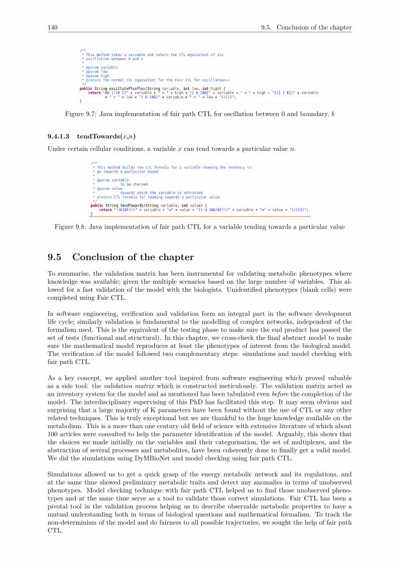
140 9.5. Conclusion of the chapter
Figure 9.7: Java implementation of fair path CTL for oscillation between 0 and boundary, b
9.4.1.3 tendTowards(x,n)
Under certain cellular conditions, a variable x can tend towards a particular value n.
Figure 9.8: Java implementation of fair path CTL for a variable tending towards a particular value
9.5 Conclusion of the chapterTo summarise, the validation matrix has been instrumental for validating metabolic phenotypes whereknowledge was available; given the multiple scenarios based on the large number of variables. This al-lowed for a fast validation of the model with the biologists. Unidentified phenotypes (blank cells) werecompleted using Fair CTL.
In software engineering, verification and validation form an integral part in the software developmentlife cycle; similarly validation is fundamental to the modelling of complex networks, independent of theformalism used. This is the equivalent of the testing phase to make sure the end product has passed theset of tests (functional and structural). In this chapter, we cross-check the final abstract model to makesure the mathematical model reproduces at least the phenotypes of interest from the biological model.The verification of the model followed two complementary steps: simulations and model checking withfair path CTL.
As a key concept, we applied another tool inspired from software engineering which proved valuableas a side tool: the validation matrix which is constructed meticulously. The validation matrix acted asan inventory system for the model and as mentioned has been tabulated even before the completion of themodel. The interdisciplinary supervising of this PhD has facilitated this step. It may seem obvious andsurprising that a large majority of K parameters have been found without the use of CTL or any otherrelated techniques. This is truly exceptional but we are thankful to the huge knowledge available on themetabolism. This is a more than one century old field of science with extensive literature of which about100 articles were consulted to help the parameter identification of the model. Arguably, this shows thatthe choices we made initially on the variables and their categorisation, the set of multiplexes, and theabstraction of several processes and metabolites, have been coherently done to finally get a valid model.We did the simulations using DyMBioNet and model checking using fair path CTL.
Simulations allowed us to get a quick grasp of the energy metabolic network and its regulations, andat the same time showed preliminary metabolic traits and detect any anomalies in terms of unobservedphenotypes. Model checking technique with fair path CTL helped us to find those unobserved pheno-types and at the same time serve as a tool to validate those correct simulations. Fair CTL has been apivotal tool in the validation process helping us to describe observable metabolic properties to have amutual understanding both in terms of biological questions and mathematical formalism. To track thenon-determinism of the model and do fairness to all possible trajectories, we sought the help of fair pathCTL.

141 9.5. Conclusion of the chapter
Finally, our mathematical model is a formal model of the metabolic regulation in eukaryotes. As themetabolic network is a central machinery for cell proliferation, our proposed model can be integrated inmore complex and large networks (more parametrisation will be required) including, in particular, celldivision cycle. These models are of interest for studying the control of cell proliferation (for examplecancer, parasite related diseases, etc). We give some fruitful applications where our model is being usedin the next final chapter.
CHAPTER 10CONCLUSION
This manuscript demonstrated the interdisciplinary work needed for the logical modelling of the regulationof the metabolic pathways : a contribution brought together by computer scientists and biochemists. Themain contributions of the thesis are reminded in this chapter; we then show how our model could be usedas input for other projects and discuss the main possible avenues for future works.
10.1 Contributions of the thesisWe have achieved a rather big and intricated model of central carbon metabolism to understand the reg-ulation mechanisms that control the metabolic shift between respiration and fermentation. This modelincludes several novative abstractions, without which it would not be possible to manage the modellingtask, due to a large number of interdependent variables. As a result, we obtain a fully consistent abstractmodel that offers a "global view" never offered up to now within a fully mathematically defined modelwith dynamics. This finds many interesting applications as this model is pluggable in metabolic relatedresearch (for example in cancer therapy).
The choice of a discrete model has been decisive in the success of our modelling objective. This choicealso is somehow "non-standard" in a domain (metabolism) where all models are based on quantitativeflux modelling. Owing to this choice, we have been able to provide a coarse-grained model able to mimicthe metabolic network behaviour. The model uses sufficiently global components of energetic metabolismin order to identify parameters through global understanding of these components (metabolic pathways).As a result, it has been possible to determine all regulation kinetic parameters K which basically informthe cellular component or pathway which action to make according to input signals (sometimes a combi-nation of activation and inhibitory signals).
We have put in place a well-defined methodology to tackle the degree of complexity of the metabolicnetwork. This comprises of two parts : first, the K parameters have been determined using a set of"thought experiments" supported by a large number of biochemical knowledge, supplemented secondlyby using a "validation matrix" which exposes a systemic view of the expected global behaviour of themodel.
The model has been validated using proof checking techniques from software engineering that wereapplied to the R. Thomas formalism. Validation of experimental phenotype has been possible using Com-putation Tree Logic (more precisely Fair path CTL) which assesses whether an experimental phenotypelisted in a validation matrix is reachable by the model or not at a certain time in the future.
We developed the software platform DyMBioNet according to the aforementioned methodology. DyM-BioNet was essential to put in place a software environment to easily manage all the 14 variables (and100 K parameters) and also to observe the overall dynamics of the system. Thus, we constructed theDyMBioNet platform for simulation purposes as well as to check a host of Fair CTL properties.
10.1.1 Contribution to theoretical biologyDue to the high complexity of biological networks, one often needs to abstract from the structural specificsof a mechanism and represents it in a skeletal, coarse-grained manner. There is a lot of biologicalresearches that have been successful for the study of gene and protein networks by applying a certaindegree of abstraction [159]. In doing so, we lost information on molecular details but however, we gainedsufficient precision on the phenotypic behaviour of the different metabolic pathways and their regulations.
142
143 10.1. Contributions of the thesis
This central notion of abstraction presents powerful strategies where the causal relationships can beidentified. By using this mindset, we have successfully been able to abstract the pathways regulating theproduction of energy and biomass: two pivotal elements for cell survival and proliferations. We show thisabstraction as follows:
• the ability to regroup biological entities in different cell compartiments. For example, we haveabstracted two main cofactors ATP and NADH present in cytosol and mitochondria.
• the ratio of ATP/ADP and NADH/NAD+ have been regrouped in only one variable ATP andNADH respectively. ADP is represented as ¬ATP and NAD as ¬NADH. At the same time, ATP(respectively NADH) also abstract their derivatives GTP (respectively NADPH).
On this understanding of abstraction, this has allowed us to reduce drastically the number of variablesand build a minimised version of the metabolic regulatory graph. Modelling the dynamic behaviour ofthe metabolic network could have taken two forms either using classical continuous frameworks or usinga discrete approach. We opted for the discrete dynamical approach and we give our justifications in thenext sub-section.
10.1.2 Modelling strategyFor a long time, differential equations have been the classical choice for the study of biological systems.However, differential equations present a major difficulty: The set of parameter values must be deter-mined from curve fitting that ask for many experiments with precise measurements. The number of realparameters is comparable to the number of discrete parameters of our approach but they can take aninfinity number of real values, making their identification far more complex.
We illustrate this by assuming we have the in-degree (number of variables acting on it) of a variableset to n, which in differential equation would lead to 2n + 2 parameters. In our model, most of thein-degrees n lies between 2 and 3, and as we have seen (in chapter 4), the use of multiplexes greatlyreduces the number of in-degree for each variable. If we were to use differential equations, the numberof kinetic parameters for n would therefore lies between 6 and 8. In the discrete logical approach, onaverage, n is between 4 and 8. The difference in numbers of parameters is not significant in the twoapproaches. But, the discrete formal approach only requires finding discrete finite values (0 to 2) whereasfinding continuous values in differential equation is far more difficult with a larger domain. Finding thesevalues from learning techniques based on heuristics depend heavily on the amount of data as input andmore often, most of these precise data is unknown. Therefore, this allows for only a partial identificationof parameters with differential equations. On the contrary, by selecting an abstract level of intervals, ourlogical approach allows for an exhaustive search in the identification of K parameters.
We used Thomas’ framework, as a large majority of interactions are of regulatory nature. We thought theidentification of integer parameters would be easier than any continuous approach as we would benefitfrom the use of model checking tools. Even better, after completing the model, we realised that notonly the boundary for almost all variables lies between 0 and 2 but also the in-degree for almost allvariables is less than 3. This gives rise to a fairly smaller number of kinetic parameters to identify, com-pared to differential equations, and this reinforces a posteriori our choice for a discrete approach. As theboundary for some variables exceeds a boolean value, we opted for the multivalued Thomas alternative.Model checking technique using Fair path CTL has allowed us to easily verify known metabolic traits,and confirmed our K parameter values.
10.1.3 MethodologyPutting in place a strict methodology was pivotal for the smooth and effective progress of the thesis dueto the large complex size of the network, and also to avoid missing any regulatory paths during the coarse-grained construction of the metabolic network. On one hand, the interdisciplinary "though experiment"guided us to the determination of the 100 K-parameters with the help of the biochemist thank to theavailable rich bibliography. On the other hand, the validation matrix (inspired from software engineering)was useful for depicting the global behaviour of the model. Metabolism is a well-studied metabolic net-work, most of the known phenotypic behaviours were listed in the validation matrix. Unknown cellularbehaviour were queried using our formal checking tools.
This methodology is comparable to classic software engineering : the interaction graph and the val-ues of the K parameters determined from biochemical transitions play a similar role as a computer
144 10.1. Contributions of the thesis
program with its detailed stepwise instructions, whereas the validation matrix is comparable to a formalspecification of a program since it formalises the expected global behaviour of the model. Then, modelchecking for CTL is the tool to formally prove correctness.
Just like in software engineering practices, it is crucial to keep the independence between (1) the writingof the specification and the final testing of the product and (2) the development of the detailed program.In the same way, the independence of the K parameters identification using biochemistry knowledge andthe validation matrix by phenotypic analysis in biology, was crucial for a good quality validation of themetabolic model proposed. Compared to the thesis plan, the validation matrix was written well beforethe identification of the K parameters (therefore before testing the global behaviour of the model) by ourplatform DyMBioNet.
To end, it is important to highlight that it is the first time, to our knowledge, that this type of sys-temic methodology is being put in place for modelling in systems biology due to the size of the model,among the largest, using R. Thomas theory.
10.1.4 Verification of proposed abstract modelWe implemented two complementary ways of verifying the correctness of our model and all the underlyingregulations in the metabolic network : graphic simulations and model checking with CTL formulas.
Graphic simulations using DyMBioNet helped us for checking the model for basic regulations and well-known phenotypes (for example oscillations in certain environmental contexts) in a specific timeframe.This approach enabled us to proceed relatively fast with the model and gave us some relative guaranteethat the K parameters were good estimations. Furthermore, these simulations gave us sufficient groundsto get a base model which is easily configurable. Unfortunately, due to the large number of variables,simulations were slow and it was almost impossible to detect the behaviour of the variables in the long run.
For unknown environmental contexts and for an infinite timeframe, we revert to model checking whereunknown biological properties were verified using CTL. Due to the complexity of the network, the hugenumber of variables and the high number of retroactions, classical CTL fails to check certain properties(certain paths were never visited which means wrong interpretations of certain phenotypes). To ensureequity in all the paths, biological traces were handled using fair path CTL. This guaranteed to ignorespurious unfair paths where a given transition is neglected although its initial state is reached an infinitynumber of times. that all paths would at least be visited once an infinite number of times.
In between, we highlighted the importance of the validation matrix that allows us to cross-check dynamicproperties of the model with known biological observations. Simulations have been instrumental to getwell acquainted with the mathematical model and have been carried out with our new tool, DyMBioNet.Each simulation result was verified against the cells for a given context. For long term verifications ofvariables, complex properties in the normal CTL were translated and formalised using Fair path CTL.
Finally, we have a generic, complete and fully validated abstract model of the regulation of energyand biomass production of metabolism in eukaryotes. This generic model can serve as a blueprint forthe design of more complicated biological systems and some of these systems are discussed in the nextsection.
10.1.5 DyMBioNet : A modelling platform for Thomas’ modelsIn the context of complex biological regulation networks, we have designed a configurable software archi-tecture to deal with the dynamics of the networks. The DyMBioNet platform is a modular tool which isextensible allowing future users to easily incorporate other functionalities.
The set of existing options bundled with DyMBioNet include : a visual GUI to design a biologicalnetwork from scratch, customise K parameters, threshold values and variable colors, a charting interfacefor simulation purposes, and the possibility to visualise a 3D representation of state transition diagram ofsmall biological networks (≤ 3 variables). The tool has been instrumental for verifying known biologicalphenotypes and to go further, users can benefit from checking these same phenotypic behaviours (andunknowns as well) using Fair path CTL. Also, a reporting feature is available to generate global evolutionsof all variables under certain environmental conditions set by the user.
145 10.2. Future directions
10.2 Future directionsThe model we have developed using the R.Thomas framework allows to implement the behaviour ofdifferent types of cells. We are able to model normal cells (quiescience and / or proliferation) or toadd certain properties which are unique to cancerous cells. If our model is based only on normal cellswhich are proliferative in nature with the classic respiration-fermentation shift, the different hypothesesfor other types of cells can be realised by modifying certain K parameters.With the implementation of Fair path CTL for path equity in the model, there is the possibility todo certain phenotypic screening of cells to identify conditions necessary for the activation or inhibitionof phenotypes of interest (like fermentation). More interesting, this can enable us to find importantcombination of actions necessary to reverse the Warburg effect alongside the main metabolic pathwaysof central carbon metabolism. These combinations (which can be encapsulated in multiplexes) can betranslated into an action in poly-pharmacology (a combination of drugs) for reversing the Warburg effectand suggest novel approaches for cancer metabolism. The choice of each drug activating or inhibiting acertain metabolic pathway cannot predicted by the model. This expertise is left to the pharmacologist.Integrating our "turnkey" system into more elaborated complex models will not necessarily imply addingmany new variables and neither exploding many existing variables into subunits. Nevertheless, thebibliographical knowledge acquired from the 100 kinetic parameters can be foundational for furtherspecific contexts. This can take two twists:
• the model is controlled by other variables (on top and above what we have considered for ourcontext) which act on the existing input variables. For example, if we have an oncogene maintainingthe value of glucose to 1, this will reduce the number of parameters and will also have a cascadingeffect on the model as a whole: all multiplexes using glucose greater than 1 can be simplified, possiblybringing new constraints on some target variables, which in turn, can allow further simplifications.
• the model is merged into a more complex system where it serves as a "black box" input to othersubsystems. For example, incorporating the model with the cell cycle or the circadian clock.
We may also imagine a hybrid version of this metabolic regulation by incorporating the notion of time:that is how much time we spend in a given discrete state. But, due to the degree of abstraction, this ishardly achievable as many details are hidden in the abstracted variables. So, we do not include this as afuture work, at least before a notably long term.
This section is devoted to the list of future works entailing the regulation of energy and biomass regulationin eukaryotes. First, we give a brief explanation of an ongoing project which has already started usingour generic model and second we present other potential metabolically-engineered disciplines.
10.2.1 The project "PAIR Pancreas"This project involves 5 french research teams including I3S, INSERM Marseille, INSERM Toulouse, IN-SERM Lyon and INSERM Lille.
Cell to cell communication occurs via signalling pathways to accomplish the transmission of impor-tant biological information. This intercellular communication is complex, forming a network of networkswhere the output of one cell becomes the input of other cells. In such complexity, feedback loops canarise and there is possibility of recursivity. In cancer progression, this communication is altered wherecancer cells persuade normal cells to give unique growth signals for proliferation. These growth signalsare under the control of a family proteins known as Ras proteins (including HRas, NRas and KRas). Butit is well-known in cancer biology that, among the Ras genes, KRas is the most mutated and active gene.K-Ras orchestrates (via the energy and biomass production) ROS production which is harmful to cells.Persistent ROS generation can damage DNA and can activate p53 to promote full-blown apoptosis [166].
As such, the objectives of the PAIR pancreas project are to elucidate the communication between dif-ferent types of cells with more emphasis on KRas protein and ROS. The workflow for this project is tobetter understand cell-to-cell communication as follows: normal cells and cancer cells, normal cells andaggressive cells, and finally between normal cancer cells and aggressive cancer cells.
This study of information interchange between normal cells and cancer cells can open up new thera-peutic windows to pancreas cancer treatment.
146 10.2. Future directions
10.2.2 A rather natural continuation : Interplay between the circadian cycle,cell cycle and metabolic regulations
Cells have built-in mechanisms to sustain their activities (growth and repair) by sensing the organism’sdemand, which are controlled in a timely manner. This is to limit damage and maintain homeostasis:both important for cell’s survival and the smooth running of the organism as a whole. The state of theorganism is orchestrated by three main biological regulations: metabolism to give energy and biomass,cell cycle which integrates cell division procedures and the circadian clock which imposes a rhythm foreach process to optimise the succession of biological processes (and at the same time to optimise resourceusage).
However, highly proliferative cells impose their own rules and bypass these setups. Cancer, for ex-ample, is characterised by an uncontrolled cell growth supported by metabolic reprogramming. They donot follow the usual pathways of normal cells and more often they display abnormal cellular capacitiesthat allow them to become aggressive and dominate neighbouring cells. On top of that, they becomeresistant to the body immune systems.
This motivates to focus researches on the crossroad between the study of the three aforementioned cyclesand how their inter-communications can provide insights for chrono-therapeutics approaches for manydiseases. It would be of outmost interest to understand the dynamics between the following networks:
1. Metabolism and cell cycleThe metabolic requirements of dividing cells differ largely from that of resting cells: they need toreplicate their DNA and need more biomass [176, 177]. This means that cell cycle progression ishighly dependent on metabolism which itself relies on substantial nutrients supply. Evidence isemerging in support of the coordinated temporal regulation of metabolism directly by the cell cyclemodulators [175].
2. Cell cycle and Circadian cycleRecent research has shown that a disruption of the circadian timing system in mice causes increasedtumour development [174]. The formal regulation of the circadian cycle on the cell cycle imple-mented using a mathematical model can provide a precise understanding of this intuitive mechanics.This can open doors for precise medicines to revert the uncontrolled proliferative properties of can-cer cells. For example, there is a possibility to target specific times when cancer patients can beadministrated medicines for sustaining health.
3. Circadian cycle and metabolismCircadian rhythms and cellular metabolism are intimately linked [171]. Multiple systemic andmolecular mechanisms exist that connect the circadian clock with metabolism at all levels, fromcellular organelles to the whole organism, and deregulation of this circadian-metabolic crosstalk canlead to various pathologies [172].
10.2.3 Research opportunities other than diseasesMany micro organisms and plants display metabolic properties that offer potential for commercial appli-cations [160, 161]. We discuss two emerging metabolic-engineered processes as follows:
• BiodegradationThere is a global concern on the accumulation of all forms of plastics as environmental wastes. Manystrategies are being adopted worldwide to ban plastics and use paper as alternatives. Syntheticplastics, which are widely present in materials of everyday use, are ubiquitous and slowly-degradingpolymers in environmental wastes [162]. Some species of Pseudomonas have shown great efficiencyfor degrading polluants including plastics, oils and other types of polymers. These kind of bio-remediations through metabolic engineering are useful for a sustainable environment and should beused at a larger scale. A better way of achieving this, is to modulate the existing generic metabolicmodel to identify ways of increasing the biomass yield in a short duration.
• BiofuelsThe efficient production of biofuels like bioethanol, biohydrogen and biodiesel are safer alternativesfor a greener environment as they have shown cleaner burning characteristics. They can significantlyreduce the emissions of greenhouse gases and are considered as replacements for many petroleumsproducts. Recently, microorganisms are being metabolically engineered to convert carbon elements(example carbon dioxide) to effective biochemicals [164, 165]. In these processes, many parameters

147 10.2. Future directions
can be tuned to enhance fuel production.
In short, we believe that energy and biomass form the left and right hands of the cell: both are neededto carry out all the activities for continual existence of the cell. In this study, we have modelled part ofthe whole mesh of networks in metabolism: the regulation of the energy and biomass production. Thestudy of the metabolism is complex, yet exciting. It has just started and we hardly know how manyapplications and discoveries will be unraveled in the future.

List of Figures
2.1 Anabolism and catabolism are mutually exclusive: catabolism degrades biomass to produceenergy and anabolism does the reverse by consuming ATP. . . . . . . . . . . . . . . . . . 6
2.2 Glycolysis: A catabolic process producing ATP, NADH and pyruvate, and some precursorsfor Pentose Phosphate Pathway (PPP) . . . . . . . . . . . . . . . . . . . . . . . . . . . . . 9
2.3 GADPH plays a double role in cytoplasmic metabolism: Glycolytic (conversion of NAD+to NADH) and non-glycolytic (conversion of NADPH to NADP+) . . . . . . . . . . . . . 9
2.4 A brief summary of PPP: Oxidative decarboxylation occurs where G6P is converted inintermediate steps to Ribose-5-Phosphate (R5P). Depending on cell demands, R5P caneither route to the oxidative branch to support biomass production through nucleotidesynthesis. In starve conditions, R5P is converted into intermediates F6P and G3P to bereused in reverse glycolysis. . . . . . . . . . . . . . . . . . . . . . . . . . . . . . . . . . . . 11
2.5 Positive regulation on the left and negative regulation on the right [10] . . . . . . . . . . . 112.6 Metabolic loop between glycolysis and fermentation in mammalian cells . . . . . . . . . . 112.7 Summary of the different steps in oxidative krebs. Source: [27] . . . . . . . . . . . . . . . 132.8 Proteins complexes (I to IV) transferring electrons in Oxidative Phosphorylation. [28] . . 142.9 Efficient (respiration) versus inefficient catabolism (fermentation) [29] . . . . . . . . . . . 152.10 Overview of anabolic activities. Biomass synthesis from 1) Nucleotides for DNA and 2)
Acetyl-CoA for fatty acids . . . . . . . . . . . . . . . . . . . . . . . . . . . . . . . . . . . . 152.11 Alternating expression of anabolic and catabolic genes. The top panel shows the time
courses of the dissolved O2 trace (DOT) in the culture medium in percent of the saturatedconcentration. (Figure taken from [13]). Catabolic and anabolic activities are mutuallyexclusive as we have shown in Figure 2.1; when one is low, the other activity is high. . . . 17
2.12 Malate-Aspartate shuttle: Malate is converted into oxaloacetate in the oxidative phaseof TCA cycle. Some oxaloacetate molecules escape through the mitochondrial membraneinto the cytosol in the form aspartate. . . . . . . . . . . . . . . . . . . . . . . . . . . . . . 18
2.13 Citrate-pyruvate shuttle: Pyruvate can be converted to Acetyl-CoA which moves out ofthe mitochondria and enters the cytoplasm as citrate . . . . . . . . . . . . . . . . . . . . . 18
2.14 Our proposed regulation graph. It summarises, at a coarse grained level, the diverseregulations mentioned in this chapter. . . . . . . . . . . . . . . . . . . . . . . . . . . . . . 19
3.1 Enzymatic reaction : A dotted arrow meaning a reversible reaction. . . . . . . . . . . . . 203.2 Enzymatic reaction: B remains unchanged after the conversion of A to C. . . . . . . . . . 223.3 Toy example of a metabolic network : u and v are substrates; d and e are products; b and
c are internal metabolites . . . . . . . . . . . . . . . . . . . . . . . . . . . . . . . . . . . . 223.4 An example of a toy network (left) with four external metabolites: A as input, and C, E
and F as outputs. Three elementary modes (X, Y and Z) are extracted from the network,with stoichiometric coefficients on the arrows. This figure will be used to illustrate howthe three EMs participate to produce a certain flux of interest. . . . . . . . . . . . . . . . 27
3.5 Elementary mode 1 (EM1): 2X + Z; there is no need to have Y in the computational pathsas we target only the flux distribution of C and F. . . . . . . . . . . . . . . . . . . . . . . 28
3.6 Elementary mode 2 (M2): 2X + 1/2 Y + 1/2 Z; an equal distribution of weight betweenY and Z allows us to produce the required metabolic phenotypes shown in (a) . . . . . . . 28
3.7 Elementary mode 3 (EM3): 2X + 1/8 Y + 3/8 Z; we need to put a greater weight of F inZ to be able to achieve the output shown in (a). . . . . . . . . . . . . . . . . . . . . . . . 29
3.8 A simple enzymatic reaction of the conversion of substrate(S) to product(P) catalysed byan enzyme(E). kf , kr and kenz are rate constants. C denotes an intermediate reaction. . . 30
3.9 Interaction graph between gene x and gene y. x activates y and y inhibits x . . . . . . . . 313.10 A sigmoid representing the action of x on y. Here, we have a positive sigmoid demonstrating
activation. x will gradually increase the derivation of the expression level of y over time. . 313.11 A sigmoid representing the action of y on x. A negative sigmoid demonstrating inhibition
where y decreases the derivation of the expression level of x over time. . . . . . . . . . . . 31
148
149 List of Figures
3.12 Curve-fitting in differential equation by calculating distance between model and experi-mental data. . . . . . . . . . . . . . . . . . . . . . . . . . . . . . . . . . . . . . . . . . . . . 32
3.13 Computation Tree: To explore the whole structure, we can intuitively see CTL as unwind-ing the state transition graph so that it works down the tree when validating a particularformula. . . . . . . . . . . . . . . . . . . . . . . . . . . . . . . . . . . . . . . . . . . . . . . 34
3.14 Example of a state transition graph: stable state (x=2,y=0), its attraction basin (coveringstates starting from x=0,y=0) and infinite loop (transitions between states 1,1 and 0,1) . 36
3.15 Model Checking as a black box. It takes two inputs: a state transition graph and a CTLformula, and outputs whether the CTL formula is valid or at least a state which does notsatisfy the CTL formula. . . . . . . . . . . . . . . . . . . . . . . . . . . . . . . . . . . . . . 36
3.16 Model checking using EX : All predecessors of a state labelled φ are labelled with EXφeven if they have other successors (dotted arrow). . . . . . . . . . . . . . . . . . . . . . . . 37
3.17 Model checking using EG : All states labelled with φ which are also the predecessors ofstate satisfying φ, are labelled with EGφ . . . . . . . . . . . . . . . . . . . . . . . . . . . . 37
3.18 Model checking using E(φ U ψ). (a) A state where ψ holds can be labelled as E(φ U ψ) . 373.19 (i)Boolean network showing the interaction between three variables A, B and C. (ii)
Boolean functions for expressing the type of cooperations between the variables. (iii)Truth tables for nodes A, B and C . . . . . . . . . . . . . . . . . . . . . . . . . . . . . . . 38
3.20 Boolean network - Sample synchronous transition : Only one transition for each state ispossible. . . . . . . . . . . . . . . . . . . . . . . . . . . . . . . . . . . . . . . . . . . . . . . 39
3.21 Boolean network - An example of an asynchronous transition : Many transitions possiblefor each state. . . . . . . . . . . . . . . . . . . . . . . . . . . . . . . . . . . . . . . . . . . . 39
3.22 Boolean network - An example of block synchronous transition : For instance, by allowingchanges to {A,B} followed by {C}, state 101 changes to 111 (red arrow) then stay in 111for changes in {C} as shown with blue arrow . . . . . . . . . . . . . . . . . . . . . . . . . 39
3.23 A Petri net with (i) 4 places (ii) 3 transitions (t1,t2,t3) (iii) 2 tokens in place P1 . . . . . 413.24 Incidence matrix, C, calculated using C = O - I. The incidence matrix can be read as
follows : for example if t1 fires, then 2 tokens have to be removed from p1, 1 and 2 tokensadded to p2 and p3 respectively while a "0" value means no direct transitions exist betweent1 and p4. . . . . . . . . . . . . . . . . . . . . . . . . . . . . . . . . . . . . . . . . . . . . . 41
3.25 (a) Starting from Figure 3.23, only transition t1 will fire as I(t1, p1) contains sufficientnumber of tokens from p1 to pass on to p2 (1 token) and p3 (2 tokens). (b) Only transitionst2 and t3 will be enabled and we assume t2 will fire first followed by t3 (c) Only t3 will beenabled and is the only one to fire. . . . . . . . . . . . . . . . . . . . . . . . . . . . . . . . 41
3.26 BIOCHAM : Boolean method. 3 variables generating 8 possibilities . . . . . . . . . . . . . 44
4.1 Discretisation of sigmoids (a) Activation (b) Inhibition . . . . . . . . . . . . . . . . . . . . 474.2 Interaction graph between two variables x and y and three edges : (x, y), (y, x) and (y, y) 474.3 The interaction graph of x and y with thresholds, and how their sigmoids are discretised.
Here, we assumed that the threshold of action of y on x is lower than the one of the actionof y on itself. So, the edge y → x is labelled by a "1" and the edge y → y is labelled by a "2’. 48
4.4 Labelled interaction graph with thresholds on the edges. Alternatively, (x ≥ 1) can berepresented as 1+ or simply +, (y ≥ 2) as 2+ and ¬ (y ≥ 1) as (1−) . . . . . . . . . . . . 49
4.5 State transition type (i) Synchronous: x and y in state (1,0) change values at the sametime (ii) Asynchronous: Desynchronisation of state (1,0) to allow either x or y to changevalues. The Thomas approach is asynchronous. . . . . . . . . . . . . . . . . . . . . . . . . 50
4.6 If the global K vector at the state represented here by a cube (3 variables) attracts allpoints in the direction given by the black arrow then all trajectories will cross one of thethree grey surfaces of the cube. The three coloured edges of the cube show the placeswhere continuous trajectories would modify several discrete variables at the same time.The union of the three edges is a set of points of surface 0. The probability of crossingthem in the cube is 0. . . . . . . . . . . . . . . . . . . . . . . . . . . . . . . . . . . . . . . 51
4.7 Three variables acting on x. If we know that the two variables a and b need the other oneto act on x, we group them in a multiplex (right). . . . . . . . . . . . . . . . . . . . . . . 52
4.8 Multiplex notation: dotted arrows are used for variables involved in the logical formulawith the name of the multiplex in block letters . . . . . . . . . . . . . . . . . . . . . . . . 52
4.9 Multiplexes with logical formulas and names: multiplex C is prefixed with a negationmeaning it is an inhibition. The multiplex COMPLEX_AB indicates that a and b areactivators. . . . . . . . . . . . . . . . . . . . . . . . . . . . . . . . . . . . . . . . . . . . . . 53
4.10 An interaction graph with multiplexes as resources. ¬ means inhibition. Doted lines areonly drawn to facilitate the global view: They can be deduced from the multiplex formulas. 53
150 List of Figures
4.11 The individual reaction of x over z and y over z are merged into a multiplex with a logicalformula. . . . . . . . . . . . . . . . . . . . . . . . . . . . . . . . . . . . . . . . . . . . . . . 54
4.12 Separate multiplexes are incorporated in the regulatory graph: one for activation and onefor inhibition (prefixed by a ¬ sign) . . . . . . . . . . . . . . . . . . . . . . . . . . . . . . . 54
4.13 Interaction graph between x, y and z: y activates z which in turn activates x. This clearlymeans that y indirectly activates x. If z does not have any other biological relevance in thegraph (and it does not influence other variables), it can be replaced simply by a multiplex(M3). For sure, y could have been chosen instead of z and the choice of multiplex vsvariable is a matter of modelling choice. . . . . . . . . . . . . . . . . . . . . . . . . . . . . 54
4.14 One counter-example of Snoussi’s condition. x (respectively y) produces a protein X(respectively Y ). Alone X or Y activates z but their products produces another complexX-Y that does not activate z. So, in presence of x, the "activator" y appears to be aninhibitor because it captures the activator X without activating z. . . . . . . . . . . . . . 56
4.15 Unsatisfiability in the set of resources. {M1,M2} and {M1,M3} cannot be considered asresources. . . . . . . . . . . . . . . . . . . . . . . . . . . . . . . . . . . . . . . . . . . . . . 56
4.16 State transition graph showing the dynamics of x and y. Oscillation between x and ybetween their respective thresholds of 0 and 1. . . . . . . . . . . . . . . . . . . . . . . . . 57
4.17 (i) Only activators (ii) Only inhibitors . . . . . . . . . . . . . . . . . . . . . . . . . . . . . 584.18 Basin of attractions (i) For (+,+) cycle (ii) For (−,−) cycle (white areas) . . . . . . . . . 584.19 Negative circuit can generate oscillations. Black lines for x activates y and y inhibits x.
Red dotted lines for x acting as inhibitor on y and y is an activator of x. . . . . . . . . . . 58
5.1 (a) z is acting as a "relay" between x and y (b)z is removed as it has no outgoing edge toother variables in the system. . . . . . . . . . . . . . . . . . . . . . . . . . . . . . . . . . . 64
5.2 Introducing the input variable c . . . . . . . . . . . . . . . . . . . . . . . . . . . . . . . . . 645.3 (a) Using outgoing edges to identify thresholds for each variable. (b) x → y1 and x → y2
have the same thresholds and therefore are grouped together. . . . . . . . . . . . . . . . . 655.4 Finding the threshold for the variable x. Assuming the action of x over yi arrives before
that of yj . We must avoid seeing the interaction of the variable yi on yj , when determiningthe threshold of x over yj . . . . . . . . . . . . . . . . . . . . . . . . . . . . . . . . . . . . . 65
5.5 After identifying the thresholds, we obtain an interaction graph showing the thresholdvalue on all edges between variables. . . . . . . . . . . . . . . . . . . . . . . . . . . . . . . 65
5.6 Predecessors of y. If there are no cooperation between the predecessors, then y will have2n possible set of resources. . . . . . . . . . . . . . . . . . . . . . . . . . . . . . . . . . . . 66
5.7 The presence of both xi and xj are needed to activate y. . . . . . . . . . . . . . . . . . . . 665.8 The inhibitor xk has a greater influence than the two activators xi and xj . . . . . . . . . . 665.9 Validation matrix with x and y as main variables, c as boolean input variable; x<2 and
x=2 representing the initial states. ’→’ means tends towards a particular value; OSC(0,1)means oscillation between 0 and 1. . . . . . . . . . . . . . . . . . . . . . . . . . . . . . . . 67
5.10 Considering the variable u and all the resources(r1 and r2) acting on it. Each resource rhas a logical formula which is satisfied or not. . . . . . . . . . . . . . . . . . . . . . . . . . 68
5.11 Representing all the targets of u and their corresponding thresholds according to the knowl-edge of the network. . . . . . . . . . . . . . . . . . . . . . . . . . . . . . . . . . . . . . . . 69
5.12 Regrouping all outgoing edges having same threshold. . . . . . . . . . . . . . . . . . . . . 695.13 For identifying the K parameters for u; feedback loops (top and bottom red arrows) must
not be considered during the thought experiment. . . . . . . . . . . . . . . . . . . . . . . . 695.14 Identifying the K parameters for u; intermediate variable w must not be considered. In-
direct variables are also ignored (x acting on mult1) during the thought experiment. . . . 695.15 No resources acting on u. . . . . . . . . . . . . . . . . . . . . . . . . . . . . . . . . . . . . 705.16 Observing the effect of r1 only on u. We must not consider r2 as a resource of u. . . . . . 705.17 Observing the effect of r2 on u. We must not consider r1 as a resource of u. . . . . . . . . 705.18 Considering both r1 and r2 as resources. . . . . . . . . . . . . . . . . . . . . . . . . . . . . 715.19 Oscillation of x and y in the absence of c (c=0). . . . . . . . . . . . . . . . . . . . . . . . . 725.20 Oscillation of x and y in the presence of c (c=1) but stable state is reached immediately. . 725.21 Oscillation of x and y in the presence of c (c=1). Due to non-determinism, we can wait a
long time to see the transition from x=1 to x=2 . . . . . . . . . . . . . . . . . . . . . . . 725.22 Non-determinism: one or more trajectories may never be reached due to many feedback
loops from η to η1 to η9 and back, and only one trajectory from η to η10 leading to a stablestate that several simulations can miss. . . . . . . . . . . . . . . . . . . . . . . . . . . . . . 73
151 List of Figures
5.23 According to standard CTL, two possible qualitative dynamics are observed with a bifur-cation occurring at x = 1, y = 0. First, the blue oscillation means we can stay infinitelyin the loop and a second possibility of attaining the stable state (via the red arrows). Theoscillatory behaviour is unfair, as it neglects a possible transition an infinite number oftimes. . . . . . . . . . . . . . . . . . . . . . . . . . . . . . . . . . . . . . . . . . . . . . . . 73
5.24 CTL fairness : In this example, if we leave the system dynamics for a long time, webiologically consider that Z will eventually reach its value 1. But, the CTL formula AF(AG (z = 1)) returns false since there is possibility to stay in the plan Z=0 for an infinitenumber of transitions. . . . . . . . . . . . . . . . . . . . . . . . . . . . . . . . . . . . . . . 74
5.25 Oscillation of variable glyc between 0 and 1 : Fair path CTL conversion into normal CTLequivalent . . . . . . . . . . . . . . . . . . . . . . . . . . . . . . . . . . . . . . . . . . . . . 75
5.26 Standard CTL equivalent of fair path CTL for oscillation between 0 and n (n > 1). . . . . 755.27 Standard CTL equivalent of fair path CTL of the variable x tending towards a specific
threshold (here 2). . . . . . . . . . . . . . . . . . . . . . . . . . . . . . . . . . . . . . . . . 75
6.1 User interfaces of GINSim. The tool allows to create a new network, import as well as saverecently created networks (top left). Each node in the network can be configured with aninitial number of tokens (bottom left). Various options (synchronous, asynchronous, etc)are available to simulate the network (right). . . . . . . . . . . . . . . . . . . . . . . . . . 78
6.2 User interfaces of GNA . . . . . . . . . . . . . . . . . . . . . . . . . . . . . . . . . . . . . . 786.3 Singular states in GNA . . . . . . . . . . . . . . . . . . . . . . . . . . . . . . . . . . . . . 796.4 Interaction graph between x and y . . . . . . . . . . . . . . . . . . . . . . . . . . . . . . . 806.5 Regulation graph with multiplexes. Note that the negation sign "!" to encode sign to denote
inhibition of y over x. . . . . . . . . . . . . . . . . . . . . . . . . . . . . . . . . . . . . . . 806.6 Validation matrix for x and y with some fictitious observations. OSC means a variable
can oscillates between two given values and "→" means a variable tends towards a value.These two notions can also be encoded in CTL as we will see in Chapter 9. . . . . . . . . 81
6.7 State transition graph showing the dynamics between x and y, when c=1. . . . . . . . . . 816.8 State transition graph showing the dynamics between x and y, when c=0. . . . . . . . . . 826.9 DyMBioNet engine . . . . . . . . . . . . . . . . . . . . . . . . . . . . . . . . . . . . . . . . 836.10 Sample XML file for building the model X-Y. . . . . . . . . . . . . . . . . . . . . . . . . . 856.11 DTD sample of our model XML file. . . . . . . . . . . . . . . . . . . . . . . . . . . . . . . 876.12 XML schema sample of our model XML file . . . . . . . . . . . . . . . . . . . . . . . . . . 886.13 XML schema sample of our model XML file (continued). . . . . . . . . . . . . . . . . . . . 896.14 Creating a model from scratch with the name and description of the model. . . . . . . . . 906.15 Creating a node by specifying its attributes. . . . . . . . . . . . . . . . . . . . . . . . . . . 906.16 Creating a multiplex with its logical formula. . . . . . . . . . . . . . . . . . . . . . . . . . 906.17 SMBioNet file of the running example. . . . . . . . . . . . . . . . . . . . . . . . . . . . . . 906.18 Conversion of SMBioNet text file to its equivalent XML file in DyMBioNet using "Open-
>SMBioNet" menu. . . . . . . . . . . . . . . . . . . . . . . . . . . . . . . . . . . . . . . . 916.19 DyMBioNet to SMBioNet menu option. . . . . . . . . . . . . . . . . . . . . . . . . . . . . 926.20 Launching SMBioNet within DyMBioNet. . . . . . . . . . . . . . . . . . . . . . . . . . . . 926.21 Option to view thresholds and regulations of variables. . . . . . . . . . . . . . . . . . . . . 926.22 (Left) A multiplex where the variable X appears twice in the formula with different thresh-
olds. In this example Z has only one possible ressource (OUTZ), thus 2 parametersK_Z....(Right) Its translation into a Thomas network without multiplexes. Z has then 3 possibleressources, thus 8 parameters, and the respective values of the parameters have to reflectthe truth table of the formula of the original multiplex. . . . . . . . . . . . . . . . . . . . 93
6.23 Regulations and state transitions . . . . . . . . . . . . . . . . . . . . . . . . . . . . . . . . 936.24 Thresholds . . . . . . . . . . . . . . . . . . . . . . . . . . . . . . . . . . . . . . . . . . . . 936.25 K parameters for X and Y . . . . . . . . . . . . . . . . . . . . . . . . . . . . . . . . . . . . 946.26 Dynamics of the model XY showing evolution of X and Y based on initial conditions X=0
and Y=0. . . . . . . . . . . . . . . . . . . . . . . . . . . . . . . . . . . . . . . . . . . . . . 946.27 Network settings . . . . . . . . . . . . . . . . . . . . . . . . . . . . . . . . . . . . . . . . . 956.28 Automating simulations . . . . . . . . . . . . . . . . . . . . . . . . . . . . . . . . . . . . . 956.29 Saving charts / networks functionality . . . . . . . . . . . . . . . . . . . . . . . . . . . . . 966.30 List of useful classes/methods . . . . . . . . . . . . . . . . . . . . . . . . . . . . . . . . . . 966.31 Help menu options . . . . . . . . . . . . . . . . . . . . . . . . . . . . . . . . . . . . . . . . 976.32 Regulation graph of X , Y and C . . . . . . . . . . . . . . . . . . . . . . . . . . . . . . . . 986.33 Threshold information of X . . . . . . . . . . . . . . . . . . . . . . . . . . . . . . . . . . . 986.34 Regulatory network XYZ without multiplexes. . . . . . . . . . . . . . . . . . . . . . . . . 98
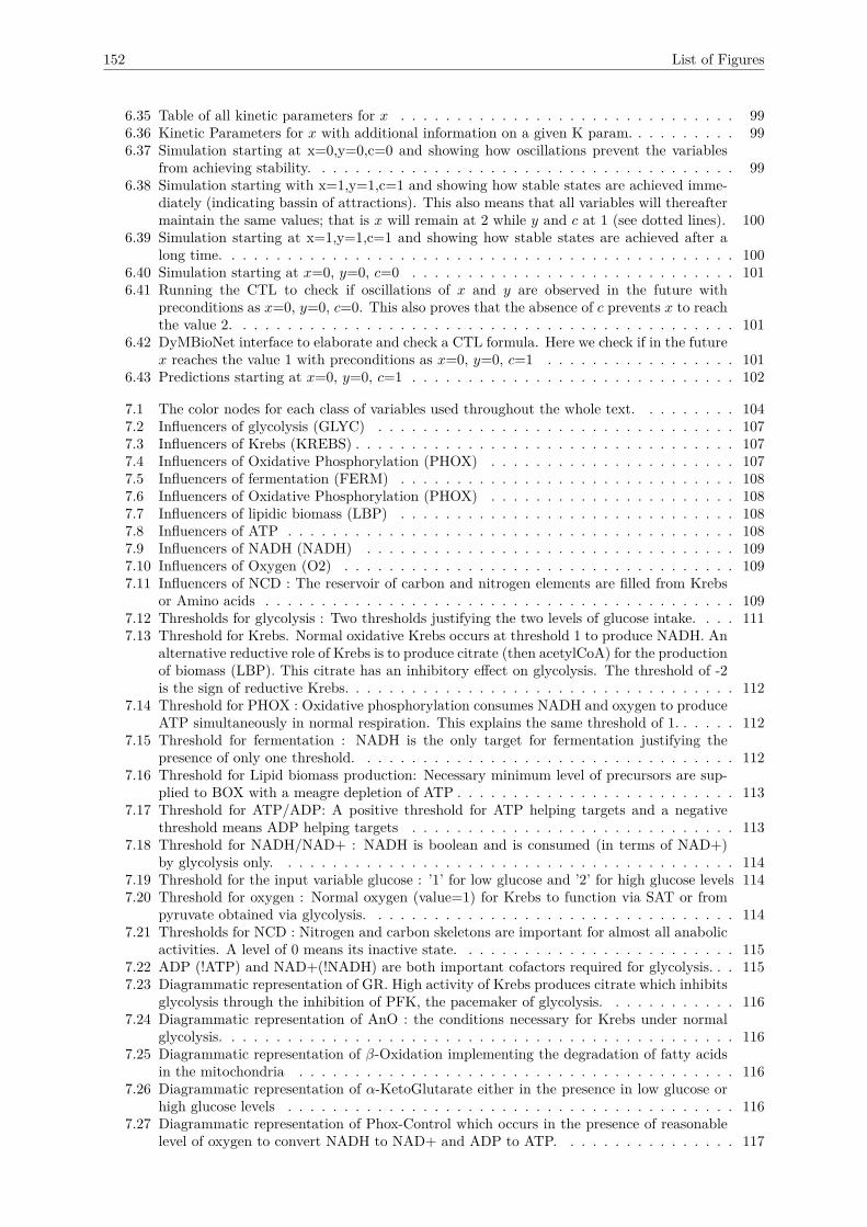
152 List of Figures
6.35 Table of all kinetic parameters for x . . . . . . . . . . . . . . . . . . . . . . . . . . . . . . 996.36 Kinetic Parameters for x with additional information on a given K param. . . . . . . . . . 996.37 Simulation starting at x=0,y=0,c=0 and showing how oscillations prevent the variables
from achieving stability. . . . . . . . . . . . . . . . . . . . . . . . . . . . . . . . . . . . . . 996.38 Simulation starting with x=1,y=1,c=1 and showing how stable states are achieved imme-
diately (indicating bassin of attractions). This also means that all variables will thereaftermaintain the same values; that is x will remain at 2 while y and c at 1 (see dotted lines). 100
6.39 Simulation starting at x=1,y=1,c=1 and showing how stable states are achieved after along time. . . . . . . . . . . . . . . . . . . . . . . . . . . . . . . . . . . . . . . . . . . . . . 100
6.40 Simulation starting at x=0, y=0, c=0 . . . . . . . . . . . . . . . . . . . . . . . . . . . . . 1016.41 Running the CTL to check if oscillations of x and y are observed in the future with
preconditions as x=0, y=0, c=0. This also proves that the absence of c prevents x to reachthe value 2. . . . . . . . . . . . . . . . . . . . . . . . . . . . . . . . . . . . . . . . . . . . . 101
6.42 DyMBioNet interface to elaborate and check a CTL formula. Here we check if in the futurex reaches the value 1 with preconditions as x=0, y=0, c=1 . . . . . . . . . . . . . . . . . 101
6.43 Predictions starting at x=0, y=0, c=1 . . . . . . . . . . . . . . . . . . . . . . . . . . . . . 102
7.1 The color nodes for each class of variables used throughout the whole text. . . . . . . . . 1047.2 Influencers of glycolysis (GLYC) . . . . . . . . . . . . . . . . . . . . . . . . . . . . . . . . 1077.3 Influencers of Krebs (KREBS) . . . . . . . . . . . . . . . . . . . . . . . . . . . . . . . . . . 1077.4 Influencers of Oxidative Phosphorylation (PHOX) . . . . . . . . . . . . . . . . . . . . . . 1077.5 Influencers of fermentation (FERM) . . . . . . . . . . . . . . . . . . . . . . . . . . . . . . 1087.6 Influencers of Oxidative Phosphorylation (PHOX) . . . . . . . . . . . . . . . . . . . . . . 1087.7 Influencers of lipidic biomass (LBP) . . . . . . . . . . . . . . . . . . . . . . . . . . . . . . 1087.8 Influencers of ATP . . . . . . . . . . . . . . . . . . . . . . . . . . . . . . . . . . . . . . . . 1087.9 Influencers of NADH (NADH) . . . . . . . . . . . . . . . . . . . . . . . . . . . . . . . . . 1097.10 Influencers of Oxygen (O2) . . . . . . . . . . . . . . . . . . . . . . . . . . . . . . . . . . . 1097.11 Influencers of NCD : The reservoir of carbon and nitrogen elements are filled from Krebs
or Amino acids . . . . . . . . . . . . . . . . . . . . . . . . . . . . . . . . . . . . . . . . . . 1097.12 Thresholds for glycolysis : Two thresholds justifying the two levels of glucose intake. . . . 1117.13 Threshold for Krebs. Normal oxidative Krebs occurs at threshold 1 to produce NADH. An
alternative reductive role of Krebs is to produce citrate (then acetylCoA) for the productionof biomass (LBP). This citrate has an inhibitory effect on glycolysis. The threshold of -2is the sign of reductive Krebs. . . . . . . . . . . . . . . . . . . . . . . . . . . . . . . . . . . 112
7.14 Threshold for PHOX : Oxidative phosphorylation consumes NADH and oxygen to produceATP simultaneously in normal respiration. This explains the same threshold of 1. . . . . . 112
7.15 Threshold for fermentation : NADH is the only target for fermentation justifying thepresence of only one threshold. . . . . . . . . . . . . . . . . . . . . . . . . . . . . . . . . . 112
7.16 Threshold for Lipid biomass production: Necessary minimum level of precursors are sup-plied to BOX with a meagre depletion of ATP . . . . . . . . . . . . . . . . . . . . . . . . . 113
7.17 Threshold for ATP/ADP: A positive threshold for ATP helping targets and a negativethreshold means ADP helping targets . . . . . . . . . . . . . . . . . . . . . . . . . . . . . 113
7.18 Threshold for NADH/NAD+ : NADH is boolean and is consumed (in terms of NAD+)by glycolysis only. . . . . . . . . . . . . . . . . . . . . . . . . . . . . . . . . . . . . . . . . 114
7.19 Threshold for the input variable glucose : ’1’ for low glucose and ’2’ for high glucose levels 1147.20 Threshold for oxygen : Normal oxygen (value=1) for Krebs to function via SAT or from
pyruvate obtained via glycolysis. . . . . . . . . . . . . . . . . . . . . . . . . . . . . . . . . 1147.21 Thresholds for NCD : Nitrogen and carbon skeletons are important for almost all anabolic
activities. A level of 0 means its inactive state. . . . . . . . . . . . . . . . . . . . . . . . . 1157.22 ADP (!ATP) and NAD+(!NADH) are both important cofactors required for glycolysis. . . 1157.23 Diagrammatic representation of GR. High activity of Krebs produces citrate which inhibits
glycolysis through the inhibition of PFK, the pacemaker of glycolysis. . . . . . . . . . . . 1167.24 Diagrammatic representation of AnO : the conditions necessary for Krebs under normal
glycolysis. . . . . . . . . . . . . . . . . . . . . . . . . . . . . . . . . . . . . . . . . . . . . . 1167.25 Diagrammatic representation of β-Oxidation implementing the degradation of fatty acids
in the mitochondria . . . . . . . . . . . . . . . . . . . . . . . . . . . . . . . . . . . . . . . 1167.26 Diagrammatic representation of α-KetoGlutarate either in the presence in low glucose or
high glucose levels . . . . . . . . . . . . . . . . . . . . . . . . . . . . . . . . . . . . . . . . 1167.27 Diagrammatic representation of Phox-Control which occurs in the presence of reasonable
level of oxygen to convert NADH to NAD+ and ADP to ATP. . . . . . . . . . . . . . . . 117
153 List of Figures
7.28 Diagrammatic representation of Excess Pyruvate (EP) in both low (absence of oxygen)and high glucose (either low or high oxygen) milieu. . . . . . . . . . . . . . . . . . . . . . 117
7.29 Diagrammatic representation of citrate showing its contribution in lipid synthesis (biomass)via AcetylCoA . . . . . . . . . . . . . . . . . . . . . . . . . . . . . . . . . . . . . . . . . . 117
7.30 Diagrammatic representation of Pentose Phosphate Pathway. We assume a normal contri-bution of all precursors in terms of energy, nitrogen and carbon skeletons. . . . . . . . . . 117
7.31 Multiplex AAS (Amino acids synthesis) : AAS obtains most of its nitrogen and carbonelements from NCD . . . . . . . . . . . . . . . . . . . . . . . . . . . . . . . . . . . . . . . 118
7.32 The proposed metabolic graph with 14 variables and 10 meaningful multiplexes. Implicitmultiplexes are not mentioned. . . . . . . . . . . . . . . . . . . . . . . . . . . . . . . . . . 119
8.1 Resources for glycolysis : Two activators COF (necessary cofactors ATP & NADH) andnoPFK (via escaped citrate from Krebs) and one input variable, GLC (at two levels : 1 or2). . . . . . . . . . . . . . . . . . . . . . . . . . . . . . . . . . . . . . . . . . . . . . . . . . 121
8.2 Resource and Target variables for NADH with associated thresholds. The resources isconstituted of 2 direct activators (KREBS and GLYC) and 3 inhibitors (AAS, PHOX andFERM). . . . . . . . . . . . . . . . . . . . . . . . . . . . . . . . . . . . . . . . . . . . . . . 122
8.3 Resources for ATP : Both PHOX and GLYC produce ATP while the production of biomass(nLBP and LBP) uses ATP. Remark that the absence of ATP is an activator of BOX. . . 125
8.4 K parameters for Krebs : On the left, a combination of three activators for the properrunning of Krebs. A level of 1 is sufficient to allow Krebs to produce enough NADH forPHOX. At level 2, Krebs has two roles : either activates lipid synthesis or regulates glucolysis.127
8.5 Resources for Oxidative Phosphorylation : Only 1 resource which encapsulates NADH andoxygen. . . . . . . . . . . . . . . . . . . . . . . . . . . . . . . . . . . . . . . . . . . . . . . 128
8.6 Resources for Fermentation : Pyruvate is a resource for fermentation . . . . . . . . . . . . 1288.7 Resources for NCD : One activator (input of AA which is a control variable at two levels
1 and 2) and KREBS as the only inhibitor at level 2 . . . . . . . . . . . . . . . . . . . . . 1298.8 Resources for non-lipidic biomass production : 2 activators and only 1 target. . . . . . . . 1298.9 Resources for Lipidic Biomass Production : 2 resources and 2 targets . . . . . . . . . . . . 1308.10 Resources for oxygen : 1 activator in the form of input of oxygen and 1 consumer which is
oxidative phosphorylation. . . . . . . . . . . . . . . . . . . . . . . . . . . . . . . . . . . . . 130
9.1 Normal Respiration with only input of glucose and oxygen. . . . . . . . . . . . . . . . . . 1379.2 Respiration with normal glucose and excess amino acids . . . . . . . . . . . . . . . . . . . 1379.3 Inactive respiration with the presence of only fatty acids and amino acids. . . . . . . . . . 1389.4 Respiration with absence of glucose milieu. . . . . . . . . . . . . . . . . . . . . . . . . . . 1389.5 Respiration with high glucose and all other nutrients present. . . . . . . . . . . . . . . . . 1399.6 Java implementation of fair path CTL for oscillation between 0 and 1 . . . . . . . . . . . 1399.7 Java implementation of fair path CTL for oscillation between 0 and boundary, b . . . . . 1409.8 Java implementation of fair path CTL for a variable tending towards a particular value . 140
11.1 General logics : Syntax defines all the allowable sets of propositions formulas that canbe stated about models. Possible Models are mathematically defined as sets where theformulas can be interpreted, allowing to define if a model satisfies a formula or not. Proofsare syntactic transformations allowing to derive new formulas from a given set of formulashypotheses via inference rules. Finally, one requires these newly inferred formulas to besatisfied in all models satisfying the hypotheses (soundness) , and where the expressivepower if weak enough, the reverse property, completeness, may be ensured. . . . . . . . . 155
11.2 Proof tree proving FERM ≤ GLYC using inference rules. Dotted lines and red text referto the leaves of the proof tree. . . . . . . . . . . . . . . . . . . . . . . . . . . . . . . . . . . 157
11.3 Temporal Semantics. (i) AX(p) : in general, p holds in all next states of a given previousstate(ii) A [p u q] : p holds until q for all cases in the tree . . . . . . . . . . . . . . . . . . 160
11.4 Temporal Semantics. (i) EF(p) : there exists a state in the future where p holds (ii) EG(p): if p holds in a state, then in general p holds in all successive states. . . . . . . . . . . . . 167
11.5 Temporal Semantics. (i) EF(p) : for a given state, there exists a next state where p holds(ii) E[p u q] : there exists a trajectory where p holds until a state where q holds . . . . . 167

List of Tables
3.1 Syntactic temporal formulas: Temporal identifiers are always preceded by quantifiers. . . 34
4.1 Table of resources for x and y using multiplexes as resources from Figure 4.10. . . . . . . 574.2 Table of K parameters for x and y. x has a maximum of two K parameters and y has a
maximum of 4 K parameters. . . . . . . . . . . . . . . . . . . . . . . . . . . . . . . . . . . 57
6.1 Information deduced from Figure 6.4. . . . . . . . . . . . . . . . . . . . . . . . . . . . . . 806.2 Table of resources from Figure 6.4.Let us remind that : (i) y is a resource of x if y is absent
(the absence of an inhibitor is a resource equivalent to the presence of an activator). Thisexplains the appearance of y in the column KX, when y=0. (ii) x is a resource of y whenit is above 1. . . . . . . . . . . . . . . . . . . . . . . . . . . . . . . . . . . . . . . . . . . . 81
7.1 List of multiplexes . . . . . . . . . . . . . . . . . . . . . . . . . . . . . . . . . . . . . . . . 1067.2 List of influencers . . . . . . . . . . . . . . . . . . . . . . . . . . . . . . . . . . . . . . . . . 110
9.1 Validation matrix for the cell metabolism regulation model. Each row (resp. column)represents an experimental condition (resp. an observable systemic variable). Thus, eachcell of the table formalises the known behaviour of that observable variable in that experi-mental condition. "osc" means oscillation with either osc(0,1) to indicate that the variableoscillates between the value 0 and 1; or osc(0,2) which means an oscillation between 0 and1, and also between 1 and 2. . . . . . . . . . . . . . . . . . . . . . . . . . . . . . . . . . . . 133
11.1 Propositional Connectives : Apart from ¬ which is a unary connective, the other connec-tives are binary . . . . . . . . . . . . . . . . . . . . . . . . . . . . . . . . . . . . . . . . . . 158
11.2 Logical Connective OR . . . . . . . . . . . . . . . . . . . . . . . . . . . . . . . . . . . . . . 15811.3 Logical Connective IMPLICATION . . . . . . . . . . . . . . . . . . . . . . . . . . . . . . . 15911.4 Logical Connective NOT . . . . . . . . . . . . . . . . . . . . . . . . . . . . . . . . . . . . . 15911.5 Natural deduction rules . . . . . . . . . . . . . . . . . . . . . . . . . . . . . . . . . . . . . 15911.6 Example of a proof tree . . . . . . . . . . . . . . . . . . . . . . . . . . . . . . . . . . . . . 160
154

CHAPTER 11ANNEX
11.1 Classical LogicsLogic is at the basis of all formal approaches. In this context, we give a panoramic view of what constitutesgeneral logics.
11.1.1 General LogicsNowadays, many modellers of complex systems are embracing logic as a useful tool to solve problems inbiology, and bioinformatics among others. Logic, which for decades, has been used in software engineeringfor validating or invalidating programs, is progressively paving its way in other areas like medicine, drugdesign and the like. A general overview of the main aspects of logic is shown in Figure 11.1 with a briefintroduction of the different parts.
Figure 11.1: General logics : Syntax defines all the allowable sets of propositions formulas that can bestated about models. Possible Models are mathematically defined as sets where the formulas can beinterpreted, allowing to define if a model satisfies a formula or not. Proofs are syntactic transformationsallowing to derive new formulas from a given set of formulas hypotheses via inference rules. Finally, onerequires these newly inferred formulas to be satisfied in all models satisfying the hypotheses (soundness) ,and where the expressive power if weak enough, the reverse property, completeness, may be ensured.
According to [?], a general logic is defined by 5 notions (sections 11.1.1.1 to 11.1.1.5) that are linkedby important properties (section 11.1.1.6):
11.1.1.1 Signatures
The first object that defines general logics is a set of possible signatures. A signature (denoted as Σ) is inpractice a set of symbols that are specific to a given studied question. We can attach static informationto each symbol and this information will establish how each symbol can be used in formulas. So, thesignature is not only the set of symbols but can also impose the arity of each symbol or typing rulesfor example. In our study, for example, the following two symbols are used among others: FERM andGLYC (representing fermentation and glycolysis respectively). Then, in our case, the corresponding staticinformation for these two symbols are : "FERM" is boolean and "GLYC" can take a maximum value of2.
155
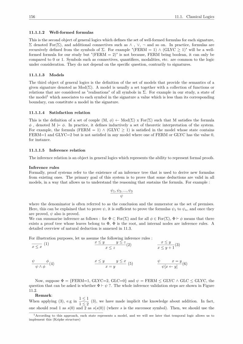
156 11.1. Classical Logics
11.1.1.2 Well-formed formulas
This is the second object of general logics which defines the set of well-formed formulas for each signature,Σ denoted For(Σ), and additional connectives such as ∧ , ∨, ¬ and so on. In practice, formulas arerecursively defined from the symbols of Σ. For example "(FERM = 1) ∧ (GLYC ≥ 1)" will be a well-formed formula for our study but "(FERM = 2)" is not because, FERM being boolean, it can only becompared to 0 or 1. Symbols such as connectives, quantifiers, modalities, etc. are common to the logicunder consideration. They do not depend on the specific question, contrarily to signatures.
11.1.1.3 Models
The third object of general logics is the definition of the set of models that provide the semantics of agiven signature denoted as Mod(Σ). A model is usually a set together with a collection of functions orrelations that are considered as "realisations" of all symbols in Σ. For example in our study, a state ofthe model1 which associates to each symbol in the signature a value which is less than its correspondingboundary, can constitute a model in the signature.
11.1.1.4 Satisfaction relation
This is the definition of a set of couple (M, φ) ← Mod(Σ) x For(Σ) such that M satisfies the formulaφ , denoted M |= φ. In practice, it defines inductively a set of theoretic interpretation of the system.For example, the formula (FERM = 1) ∧ (GLYC ≥ 1) is satisfied in the model whose state containsFERM=1 and GLYC=2 but is not satisfied in any model where one of FERM or GLYC has the value 0,for instance.
11.1.1.5 Inference relation
The inference relation is an object in general logics which represents the ability to represent formal proofs.
Inference rulesFormally, proof systems refer to the existence of an inference tree that is used to derive new formulasfrom existing ones. The primary goal of this system is to prove that some deductions are valid in allmodels, in a way that allows us to understand the reasoning that sustains the formula. For example :
ψ1, ψ2, ..., ψ3
ψ
where the denominator is often referred to as the conclusion and the numerator as the set of premises.Here, this can be explained that to prove ψ, it is sufficient to prove the formulas ψ1 to ψn, and once theyare proved, ψ also is proved.We can summarise inference as follows : for Φ ⊂ For(Σ) and for all φ ∈ For(Σ), Φ ` φ means that thereexists a proof tree whose leaves belong to Φ, Φ is the root, and internal nodes are inference rules. Adetailed overview of natural deduction is annexed in 11.3.
For illustration purposes, let us assume the following inference rules :
x ≤ x(1) x ≤ y y ≤ z
x ≤ z(2) x ≤ y
x ≤ y + 1 (3)
ψ φ
ψ ∧ φ(4)
x ≤ y y ≤ xx = y
(5) ψ x = y
ψ[x← y] (6)
Now, suppose Φ = {FERM=1, GLYC=2, GLC=0} and ψ = FERM ≤ GLYC ∧ GLC ≤ GLYC, thequestion that can be asked is whether Φ ` ψ ?. The whole inference validation steps are shown in Figure11.2.
Remark:When applying (3), e.g in 1 ≤ 1
1 ≤ 2 (3), we have made implicit the knowledge about addition. In fact,one should read 1 as s(0) and 2 as s(s(0)) (where s is the successor symbol). Then, we should use the
1According to this approach, each state represents a model, and we will see later that temporal logic allows us toimplement this (Kripke structure)
157 11.1. Classical Logics
Figure 11.2: Proof tree proving FERM ≤ GLYC using inference rules. Dotted lines and red text refer tothe leaves of the proof tree.
inference rule (3) under the more detailed (but less intuitive) form x ≤ yx ≤ s(y) .
Note that proof trees are not the only way to define "`". For example, if the set of models is finiteand if there exists a model checking algorithm able to decide if M |= ψ whatever M and ψ, then Φ ` ψcan be defined by checking all models.
11.1.1.6 Important logic properties
There are few properties that allow to evaluate the pragmatic usefulness of a logic:
• Soundness is always requiredAn inference relation is called sound, if all what we can prove is valid. More precisely : for allsignatures Σ, all subsets Φ ⊂ for(Σ) and all formulas ψ ∈ for(Σ), we have:
– if Φ ` φ then for all models M ∈ Mod(Σ), if M |= Φ then M |= ψ (where M |= Φ means :∀φ ∈ Φ,M |= ψ)
• Completeness is the reverse propertyFor all signatures Σ, all subsets Φ ⊂ For(Σ) and all formulas φ ∈ For(Σ), we have:
– If for all models M ∈Mod(Σ) : (M |= Φ) =⇒ (M |= φ), then Φ ` φCompleteness is difficult to obtain and there are several interesting logics that are incomplete.In fact, due to the Gödel theorem, a logic with recursivity is likely to be incomplete.
• DecidabilityThis simply means that there exists an algorithm which always finds the proof tree if it exists, orelse fails, in finite time.
In the next section, we give an insight on propositional logic, which is mostly the basic case of almostall logics.
11.1.2 Propositional LogicIn the past, diverse logics have been studied by philosophers, mathematicians and computer scientists.The simplest one is propositional logic. It is a logic which consists of a finite set of statements (calledatoms) which constitute the signature and can be either true or false within a model. One can constructmore complex statements using logical connectives.
11.1.2.1 Syntax
The language of propositional logic is inductively defined as follows:
• There is a finite set P = {p1, .., pn} of propositions where pi is an atomic proposition formula (P isthe signature)
• If φ is a propositional formula, then ¬φ (the negation of φ) is also a propositional formula.
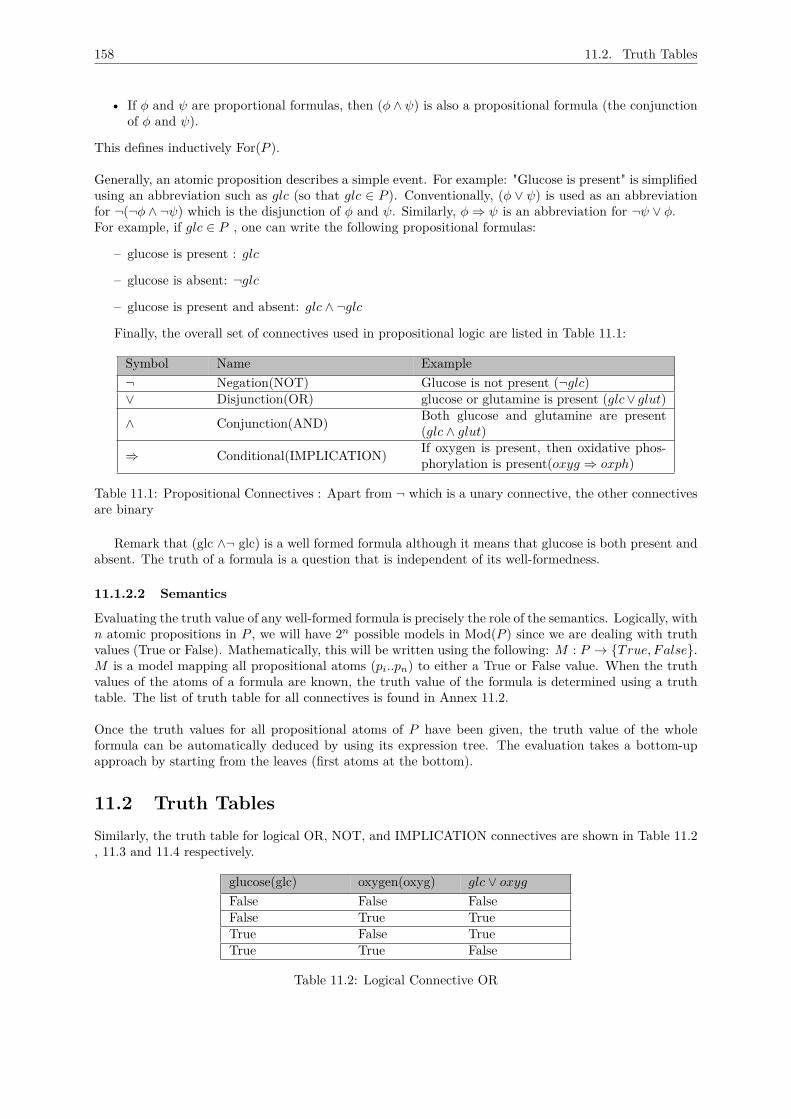
158 11.2. Truth Tables
• If φ and ψ are proportional formulas, then (φ ∧ ψ) is also a propositional formula (the conjunctionof φ and ψ).
This defines inductively For(P ).
Generally, an atomic proposition describes a simple event. For example: "Glucose is present" is simplifiedusing an abbreviation such as glc (so that glc ∈ P ). Conventionally, (φ ∨ ψ) is used as an abbreviationfor ¬(¬φ ∧ ¬ψ) which is the disjunction of φ and ψ. Similarly, φ⇒ ψ is an abbreviation for ¬ψ ∨ φ.For example, if glc ∈ P , one can write the following propositional formulas:
– glucose is present : glc
– glucose is absent: ¬glc
– glucose is present and absent: glc ∧ ¬glc
Finally, the overall set of connectives used in propositional logic are listed in Table 11.1:
Symbol Name Example¬ Negation(NOT) Glucose is not present (¬glc)∨ Disjunction(OR) glucose or glutamine is present (glc∨ glut)
∧ Conjunction(AND) Both glucose and glutamine are present(glc ∧ glut)
⇒ Conditional(IMPLICATION) If oxygen is present, then oxidative phos-phorylation is present(oxyg ⇒ oxph)
Table 11.1: Propositional Connectives : Apart from ¬ which is a unary connective, the other connectivesare binary
Remark that (glc ∧¬ glc) is a well formed formula although it means that glucose is both present andabsent. The truth of a formula is a question that is independent of its well-formedness.
11.1.2.2 Semantics
Evaluating the truth value of any well-formed formula is precisely the role of the semantics. Logically, withn atomic propositions in P , we will have 2n possible models in Mod(P ) since we are dealing with truthvalues (True or False). Mathematically, this will be written using the following: M : P → {True, False}.M is a model mapping all propositional atoms (pi..pn) to either a True or False value. When the truthvalues of the atoms of a formula are known, the truth value of the formula is determined using a truthtable. The list of truth table for all connectives is found in Annex 11.2.
Once the truth values for all propositional atoms of P have been given, the truth value of the wholeformula can be automatically deduced by using its expression tree. The evaluation takes a bottom-upapproach by starting from the leaves (first atoms at the bottom).
11.2 Truth TablesSimilarly, the truth table for logical OR, NOT, and IMPLICATION connectives are shown in Table 11.2, 11.3 and 11.4 respectively.
glucose(glc) oxygen(oxyg) glc ∨ oxygFalse False FalseFalse True TrueTrue False TrueTrue True False
Table 11.2: Logical Connective OR
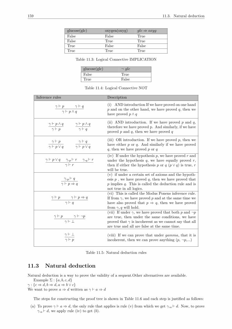
159 11.3. Natural deduction
glucose(glc) oxygen(oxyg) glc⇒ oxyg
False False TrueFalse True TrueTrue False FalseTrue True True
Table 11.3: Logical Connective IMPLICATION
glucose(glc) ¬ glcFalse TrueTrue False
Table 11.4: Logical Connective NOT
Inference rules Description
γ ` p γ ` qγ ` p ∧ q
(i) AND introduction If we have proved on one handp and on the other hand, we have proved q, then wehave proved p ∧ q
γ ` p ∧ qγ ` p
γ ` p ∧ qγ ` q
(ii) AND introduction. If we have proved p and q,therefore we have proved p. And similarly, if we haveproved p and q, then we have proved q
γ ` pγ ` p ∨ q
γ ` qγ ` p ∨ q
(iii) OR introduction. If we have proved p, then wehave either p or q. And similarly if we have provedq, then we have proved p or q
γ ` p ∨ q γ,p ` r γ,q ` rγ ` r
(iv) If under the hypothesis p, we have proved r andunder the hypothesis q, we have equally proved r,then if either the hypothesis p or q (p ∨ q) is true, rwill be true.
γ,p ` qγ ` p⇒ q
(v) if under a certain set of axioms and the hypoth-esis p , we have proved q, then we have proved thatp implies q. This is called the deduction rule and isnot true in all logics.
γ ` p γ ` p⇒ q
γ ` q
(vi) This is called the Modus Ponens inference rule.If from γ, we have proved p and at the same time wehave also proved that p ⇒ q, then we have provedfrom γ, q will hold.
γ ` p γ ` ¬pγ ` ⊥
(vii) If under γ, we have proved that both p and ¬pare true, then under the same conditions, we haveproved that γ is incoherent as we cannot say that allare true and all are false at the same time.
γ ` ⊥γ ` p
(viii) If we can prove that under gamma, that it isincoherent, then we can prove anything (p, ¬p,...)
Table 11.5: Natural deduction rules
11.3 Natural deductionNatural deduction is a way to prove the validity of a sequent.Other alternatives are available.
Example Σ : {a, b, c, d}γ : {c⇒ d, b⇒ d, a⇒ b ∨ c}We want to prove a⇒ d written as γ ` a⇒ d
The steps for constructing the proof tree is shown in Table 11.6 and each step is justified as follows:
(a) To prove γ ` a⇒ d, the only rule that applies is rule (v) from which we get γ,a ` d. Now, to proveγ,a ` d, we apply rule (iv) to get (b).
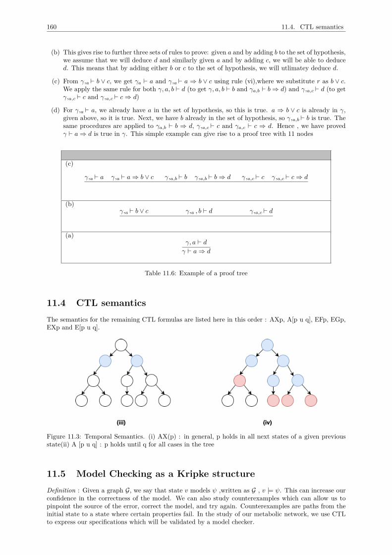
160 11.4. CTL semantics
(b) This gives rise to further three sets of rules to prove: given a and by adding b to the set of hypothesis,we assume that we will deduce d and similarly given a and by adding c, we will be able to deduced. This means that by adding either b or c to the set of hypothesis, we will utlimatey deduce d.
(c) From γ,a ` b ∨ c, we get γa ` a and γ,a ` a ⇒ b ∨ c using rule (vi),where we substitute r as b ∨ c.We apply the same rule for both γ, a, b ` d (to get γ, a, b ` b and γa,b ` b⇒ d) and γ,a,c ` d (to getγ,a,c ` c and γ,a,c ` c⇒ d)
(d) For γ,a ` a, we already have a in the set of hypothesis, so this is true. a ⇒ b ∨ c is already in γ,given above, so it is true. Next, we have b already in the set of hypothesis, so γ,a,b ` b is true. Thesame procedures are applied to γa,b ` b ⇒ d, γ,a,c ` c and γa,c ` c ⇒ d. Hence , we have provedγ ` a⇒ d is true in γ. This simple example can give rise to a proof tree with 11 nodes
(c)
γ,a ` a γ,a ` a⇒ b ∨ c γ,a,b ` b γ,a,b ` b⇒ d γ,a,c ` c γ,a,c ` c⇒ d
(b)γ,a ` b ∨ c γ,a , b ` d γ,a,c ` d
(a)γ, a ` dγ ` a⇒ d
Table 11.6: Example of a proof tree
11.4 CTL semanticsThe semantics for the remaining CTL formulas are listed here in this order : AXp, A[p u q], EFp, EGp,EXp and E[p u q].
Figure 11.3: Temporal Semantics. (i) AX(p) : in general, p holds in all next states of a given previousstate(ii) A [p u q] : p holds until q for all cases in the tree
11.5 Model Checking as a Kripke structureDefinition : Given a graph G, we say that state v models ψ ,written as G , v |= ψ. This can increase ourconfidence in the correctness of the model. We can also study counterexamples which can allow us topinpoint the source of the error, correct the model, and try again. Counterexamples are paths from theinitial state to a state where certain properties fail. In the study of our metabolic network, we use CTLto express our specifications which will be validated by a model checker.
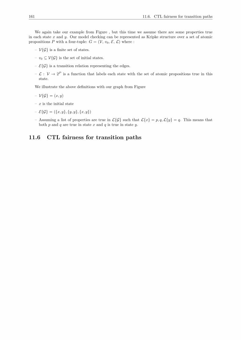
161 11.6. CTL fairness for transition paths
We again take our example from Figure , but this time we assume there are some properties truein each state x and y. Our model checking can be represented as Kripke structure over a set of atomicpropositions P with a four-tuple: G = (V, v0, E , L) where :
– V{G} is a finite set of states.
– v0 ⊆ V{G} is the set of initial states.
– E{G} is a transition relation representing the edges.
– L : V → 2P is a function that labels each state with the set of atomic propositions true in thisstate.
We illustrate the above definitions with our graph from Figure
– V{G} = (x, y)
– x is the initial state
– E{G} = ({x, y}, {y, y}, {x, y})
– Assuming a list of properties are true in L{G} such that L{x} = p, q,L{y} = q. This means thatboth p and q are true in state x and q is true in state y.
11.6 CTL fairness for transition paths
Fair paths in CTL
Adrien Richard
Laboratoire I3S - CNRS & Université de Nice
Octobre 2, 2008
1 IntroductionWe consider a Kripke structure (V,E, L) and focus on its fair paths.
Such a path p is an infinite path of (V,E) verifying : if a vertex v occursinfinitely often in p, then all the edges of E starting from v occur infinitelyoften in p. It is very natural to consider this paths when (V,E) is seen asan undeterministic discrete dynamical system whose set of states is V andsuch that : if the system is in state u at time t then the probabilities for thesystem to be in state v at time t + 1 is > 0 if (u, v) ∈ E, and 0 otherwise.Indeed, a path then describes a possible evolution of the system if and onlyif it is a fair path.
In this note, we show that all the temporal operators of the ComputationalTree Logic can be interpreted on fair paths without leave this logic. Thisallows to use the powerful computational tools related to ctl in order tocheck properties on fair paths.
2 PreliminariesThroughout this note, G = (V,E) denotes a finite directed graph in which
each vertex has at least one successor : for each u ∈ V there exists v ∈ Vsuch that (u, v) ∈ E.
A path of is a map p from N to V such that (pi, pi+1) ∈ E for all i ∈ N(the image of i by p is denoted pi). The set of images of p is denoted p(N)and is called the set of vertices of p. A path from u is a path p such thatp0 = u. A path from u to v is a path p from u such that v is a vertex of p.More generally, a path from u to A ⊆ V is a path p from u such that p hasat least one vertex in A.
In the following, we need the notions of trap domain and attractors. Antrap domain is a non-empty set A ⊆ V such that, for all (u, v) ∈ E, if
1
u ∈ A then v ∈ A. An attractor is a smallest trap domain with respect tothe inclusion relation.
Proposition 1 If u and v belong to a same attractor, then there exists apath from u to v.
proof. Suppose that u and v belong to a same attractor A. Let T be the setof w such that there exists a path from u to w. Clearly, T is a trap domainand is included in A. Since there is no trap strictly included in A, we haveA = T . So v ∈ T : there is path from u to v. �
Proposition 2 For each vertex u, there exists a path from u to an attractor.
proof. Let u ∈ V and let T be the set of v such that there exists a pathfrom u to v. Clearly, T is a trap domain, so there exists at least one attractorincluded in T . �
3 Fair pathsDefinition 1 A fair path is a path p verifying : for all (u, v) ∈ E, if thenumber of i such that pi = u is infinite, then the number of i such thatpi = u and pi+1 = v is also infinite.
Note that, from each vertex, there exists at least one fair path. Not alsothat if p is a fair path, and if p′ is a path such that there exists j such thatp′i+j = pi for all i ∈ N, then p′ is a fair path.
Remark 1 In order to see why this notion of fair path is interesting, let ussee G is seen as a discrete dynamical system : the vertex set V correspondsto the set of possible states for the system, and E corresponds to the set ofpossible transitions between states : when the system is in state u at time t+1then it is in a state v such that (u, v) ∈ E at time t+1. This usual dynamicalinterpretation can be slightly specify by stating that, when the system is instate u at time t, the probability for the system to be in state v at time t+ 1is, for all state v such that (u, v) ∈ E, strictly greater than zero. A path thendescribes a possible evolution of the system if and only if it is a fair path.
Proposition 3 Let p be a fair path, let u be a vertex of p, and let p′ be apath from u. If the number of i such that pi = u is infinite then, for all j ∈ N,the number of i such that pi = p′j is infinite.
Proof. We proceed by induction on j. If j = 0 then p′j = u and so, followingthe conditions of the proposition, the number of i such that pi = p′j = u isinfinite. If j > 0 then, by induction hypothesis, the number of i such thatpi = p′j−1 is infinite. Since p is fair, and since (p′j−1, p
′j) ∈ E, we deduce that
the number of i such that pi = p′j−1 and pi = p′j is infinite. It is then obviousthat the number of i such that pi = p′j is infinite. �
2
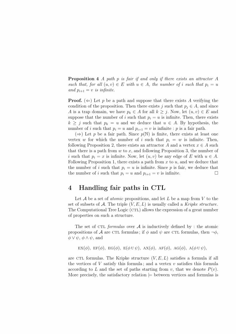
Proposition 4 A path p is fair if and only if there exists an attractor Asuch that, for all (u, v) ∈ E with u ∈ A, the number of i such that pi = uand pi+1 = v is infinite.
Proof. (⇐) Let p be a path and suppose that there exists A verifying thecondition of the proposition. Then there exists j such that pj ∈ A, and sinceA is a trap domain, we have pk ∈ A for all k ≥ j. Now, let (u, v) ∈ E andsuppose that the number of i such that pi = u is infinite. Then, there existsk ≥ j such that pk = u and we deduce that u ∈ A. By hypothesis, thenumber of i such that pi = u and pi+1 = v is infinite : p is a fair path.
(⇒) Let p be a fair path. Since p(N) is finite, there exists at least onevertex w for which the number of i such that pi = w is infinite. Then,following Proposition 2, there exists an attractor A and a vertex x ∈ A suchthat there is a path from w to x, and following Proposition 3, the number ofi such that pi = x is infinite. Now, let (u, v) be any edge of E with u ∈ A.Following Proposition 1, there exists a path from x to u, and we deduce thatthe number of i such that pi = u is infinite. Since p is fair, we deduce thatthe number of i such that pi = u and pi+1 = v is infinite. �
4 Handling fair paths in CTLLet A be a set of atomic propositions, and let L be a map from V to the
set of subsets of A. The triple (V,E, L) is usually called a Kripke structure.The Computational Tree Logic (ctl) allows the expression of a great numberof properties on such a structure.
The set of ctl formulas over A is inductively defined by : the atomicpropositions of A are ctl formulas ; if φ and ψ are ctl formulas, then ¬φ,φ ∨ ψ, φ ∧ ψ, and
ex(φ), ef(φ), eg(φ), e(φuψ), ax(φ), af(φ), ag(φ), a(φuψ),
are ctl formulas. The Kripke structure (V,E, L) satisfies a formula if allthe vertices of V satisfy this formula ; and a vertex v satisfies this formulaaccording to L and the set of paths starting from v, that we denote P (v).More precisely, the satisfactory relation |= between vertices and formulas is
3
inductively defined by : for all a ∈ A and for all ctl formula φ and ψ,
v |= a ⇐⇒ a ∈ L(v).v |= ¬φ ⇐⇒ v 6|= φ.
v |= φ ∧ ψ ⇐⇒ v |= φ ∧ v |= ψ.v |= φ ∨ ψ ⇐⇒ v |= φ ∨ v |= ψ.
v |= ex(φ) ⇐⇒ ∃p ∈ P (v), p1 |= φ.v |= ax(φ) ⇐⇒ ∀p ∈ P (v), p1 |= φ.
v |= ef(φ) ⇐⇒ ∃p ∈ P (v),∃i ∈ N, pi |= φ.v |= af(φ) ⇐⇒ ∀p ∈ P (v),∃i ∈ N, pi |= φ.
v |= eg(φ) ⇐⇒ ∃p ∈ P (v),∀i ∈ N, pi |= φ.v |= ag(φ) ⇐⇒ ∀p ∈ P (v),∀i ∈ N, pi |= φ.
v |= e(φuψ) ⇐⇒ ∃p ∈ P (v),∃j ∈ N, pj |= ψ, ∀i < j, pi |= φ.v |= a(φuψ) ⇐⇒ ∀p ∈ P (v),∃j ∈ N, pj |= ψ, ∀i < j, pi |= φ.
When (V,E) is seen as an undeterministic discrete dynamical system asin Remark 1, the set possible evolutions of the system from an initial vertexv is given by the set of fair paths starting from v, that we denote by P ′(v),and not by P (v). The ctl is then not satisfactory since a formula can befalse at v because of the paths present P (v) \P ′(v) which do not correspondto possible evolutions of the system. Typically, we can have v 6|= af(φ) whe-reas all the possible evolutions of the system from v lead to a state verifying φ.
This lead us to consider a variant of ctl, denoted ctl′, allowing theexpression of formulas interpreted according to the fair paths. More precisely,the syntax ctl′ is obtained from the one of ctl by adding the following sixtemporal operators
e′f(φ), e′g(φ), e′(φuψ), a′f(φ), a′g(φ), a′(φuψ).
The semantic of ctl′ is then obtained by adding the following equivalencesto the ones given above :
v |= e′f(φ) ⇐⇒ ∃p ∈ P ′(v),∃i ∈ N, pi |= φ.v |= a′f(φ) ⇐⇒ ∀p ∈ P ′(v),∃i ∈ N, pi |= φ.
v |= e′g(φ) ⇐⇒ ∃p ∈ P ′(v),∀i ∈ N, pi |= φ.v |= a′g(φ) ⇐⇒ ∀p ∈ P ′(v),∀i ∈ N, pi |= φ.
v |= e′(φuψ) ⇐⇒ ∃p ∈ P ′(v),∃j ∈ N, pj |= ψ, ∀i < j, pi |= φ.v |= a′(φuψ) ⇐⇒ ∀p ∈ P ′(v),∃j ∈ N, pj |= ψ, ∀i < j, pi |= φ.
4
Proposition 5 We have the following equivalences :
v |= e′f(φ) ⇐⇒ v |= ef(φ) (1)v |= a′f(φ) ⇐⇒ v |= ¬e′g(¬φ) (2)v |= e′g(φ) ⇐⇒ v |= e(φuag(φ)) (3)v |= a′g(φ) ⇐⇒ v |= ¬e′f(¬φ) (4)
v |= e′(φuψ) ⇐⇒ v |= e(φuψ) (5)v |= a′(φuψ) ⇐⇒ v |= a′f(ψ) ∧ ¬e′(¬ψ u¬φ ∧ ¬ψ) (6)
Proof. The non-obvious equivalences are the equivalences (3) and (6).To prove (3), suppose first that v |= e′g(φ), and let p ∈ P ′(v) be such
that pi |= φ for all i. Following Proposition 4, there exists an attractor Asuch that A ⊆ p(N), and we deduce that u |= φ for all u ∈ A. Let j be suchthat pj ∈ A. Since A is an attractor, for all p′ ∈ P (pj), we have p′(N) ⊆ A.So pj |= ag(φ), and since pi |= φ for all i, we deduce that v |= e(φuag(φ)).
Now, suppose that v |= e(φuag(φ)) : there exists p ∈ P (v) and j ∈ Nsuch that pj |= ag(φ) and pi |= φ for all i < j. So, given any fair pathp′ ∈ P ′(pj) we have p′i |= φ for all i ∈ N. Consider the path p′′ that weobtain by concatenating the prefix of p of length (j−1) and p′ : for all i ∈ N,p′′i = pi if i < j, p′′i = p′i−j otherwise. Clearly, p′′i |= φ for all i, and p′′0 = v.Furthermore, since p′ is a fair path, p′′ is a fair path, and we deduce thatv |= e′g(φ).
To prove (6) suppose first that v |= a′(φuψ). This obviously impliesv |= a′f(ψ). Now, suppose, by contradiction, that v |= e′(¬ψ u¬φ ∧ ¬ψ).Then, there exists p ∈ P ′(v) and j such that pj |= ¬φ and pi |= ¬ψ forall i ≤ j. So, if pk |= ψ then k > j, and since pj |= ¬φ, we deduce thatv |= ¬a′(φuψ), a contradiction.
Now, suppose that v |= a′f(ψ)∧¬e′(¬ψ u¬φ∧¬ψ). Let p ∈ P ′(v). Sincev |= a′f(ψ) there exists a smallest j such that pj |= ψ. Now, suppose, bycontradiction, that there exists i < j with pi |= ¬φ. By the choice of j, wehave pk |= ¬ψ for all k ≤ i, and we deduce that v |= e(¬ψ u¬φ ∧ ¬ψ), acontradiction. �
According to this proposition, any formula of φ of ctl′ can be translatedinto a formula ψ in ctl which is equivalent to φ, that is, such that v |=ψ ⇐⇒ v |= ψ. Furthermore, the proposition gives a constructive way toachieve this translation. This means that ctl′ formulas can be handled inpractice by the powerful verification tools related to ctl.
5
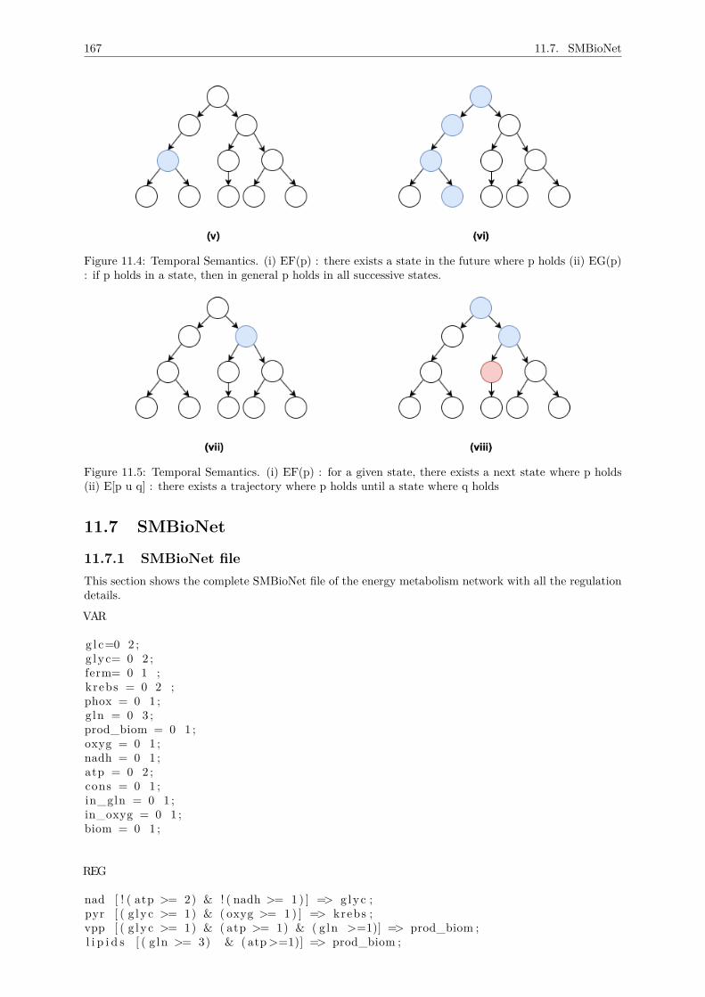
167 11.7. SMBioNet
Figure 11.4: Temporal Semantics. (i) EF(p) : there exists a state in the future where p holds (ii) EG(p): if p holds in a state, then in general p holds in all successive states.
Figure 11.5: Temporal Semantics. (i) EF(p) : for a given state, there exists a next state where p holds(ii) E[p u q] : there exists a trajectory where p holds until a state where q holds
11.7 SMBioNet
11.7.1 SMBioNet fileThis section shows the complete SMBioNet file of the energy metabolism network with all the regulationdetails.
VAR
g l c=0 2 ;g lyc= 0 2 ;ferm= 0 1 ;krebs = 0 2 ;phox = 0 1 ;g ln = 0 3 ;prod_biom = 0 1 ;oxyg = 0 1 ;nadh = 0 1 ;atp = 0 2 ;cons = 0 1 ;in_gln = 0 1 ;in_oxyg = 0 1 ;biom = 0 1 ;
REG
nad [ ! ( atp >= 2) & ! ( nadh >= 1 ) ] => glyc ;pyr [ ( g lyc >= 1) & ( oxyg >= 1 ) ] => krebs ;vpp [ ( g lyc >= 1) & ( atp >= 1) & ( gln >=1)] => prod_biom ;l i p i d s [ ( g ln >= 3) & ( atp>=1)] => prod_biom ;
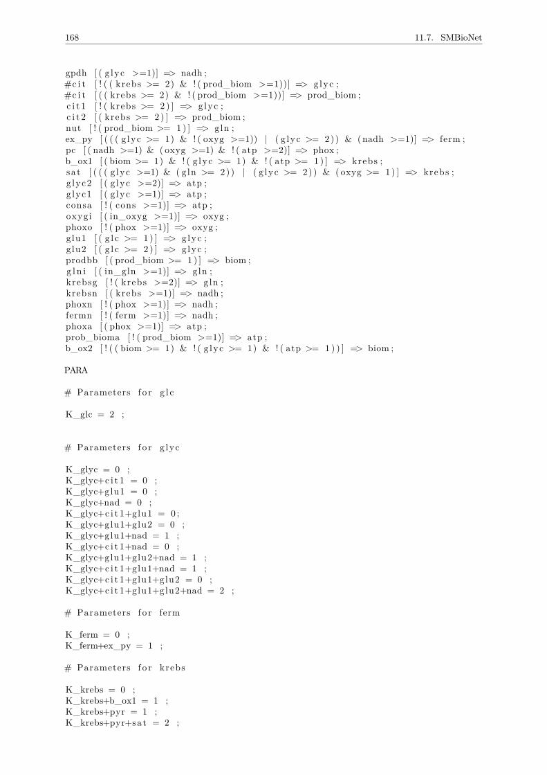
168 11.7. SMBioNet
gpdh [ ( g lyc >=1)] => nadh ;#c i t [ ! ( ( krebs >= 2) & ! ( prod_biom >=1))] => g lyc ;#c i t [ ( ( krebs >= 2) & ! ( prod_biom >=1))] => prod_biom ;c i t 1 [ ! ( krebs >= 2 ) ] => glyc ;c i t 2 [ ( krebs >= 2 ) ] => prod_biom ;nut [ ! ( prod_biom >= 1 ) ] => gln ;ex_py [ ( ( ( g lyc >= 1) & ! ( oxyg >=1)) | ( g lyc >= 2)) & (nadh >=1)] => ferm ;pc [ ( nadh >=1) & ( oxyg >=1) & ! ( atp >=2)] => phox ;b_ox1 [ ( biom >= 1) & ! ( g lyc >= 1) & ! ( atp >= 1 ) ] => krebs ;sa t [ ( ( ( g lyc >=1) & ( gln >= 2)) | ( g lyc >= 2)) & ( oxyg >= 1 ) ] => krebs ;g lyc2 [ ( g lyc >=2)] => atp ;g lyc1 [ ( g lyc >=1)] => atp ;consa [ ! ( cons >=1)] => atp ;oxygi [ ( in_oxyg >=1)] => oxyg ;phoxo [ ! ( phox >=1)] => oxyg ;g lu1 [ ( g l c >= 1 ) ] => glyc ;g lu2 [ ( g l c >= 2 ) ] => glyc ;prodbb [ ( prod_biom >= 1 ) ] => biom ;g l n i [ ( in_gln >=1)] => gln ;krebsg [ ! ( krebs >=2)] => gln ;krebsn [ ( krebs >=1)] => nadh ;phoxn [ ! ( phox >=1)] => nadh ;fermn [ ! ( ferm >=1)] => nadh ;phoxa [ ( phox >=1)] => atp ;prob_bioma [ ! ( prod_biom >=1)] => atp ;b_ox2 [ ! ( ( biom >= 1) & ! ( g lyc >= 1) & ! ( atp >= 1 ) ) ] => biom ;
PARA
# Parameters f o r g l c
K_glc = 2 ;
# Parameters f o r g lyc
K_glyc = 0 ;K_glyc+c i t 1 = 0 ;K_glyc+glu1 = 0 ;K_glyc+nad = 0 ;K_glyc+c i t 1+glu1 = 0 ;K_glyc+glu1+glu2 = 0 ;K_glyc+glu1+nad = 1 ;K_glyc+c i t 1+nad = 0 ;K_glyc+glu1+glu2+nad = 1 ;K_glyc+c i t 1+glu1+nad = 1 ;K_glyc+c i t 1+glu1+glu2 = 0 ;K_glyc+c i t 1+glu1+glu2+nad = 2 ;
# Parameters f o r ferm
K_ferm = 0 ;K_ferm+ex_py = 1 ;
# Parameters f o r krebs
K_krebs = 0 ;K_krebs+b_ox1 = 1 ;K_krebs+pyr = 1 ;K_krebs+pyr+sat = 2 ;
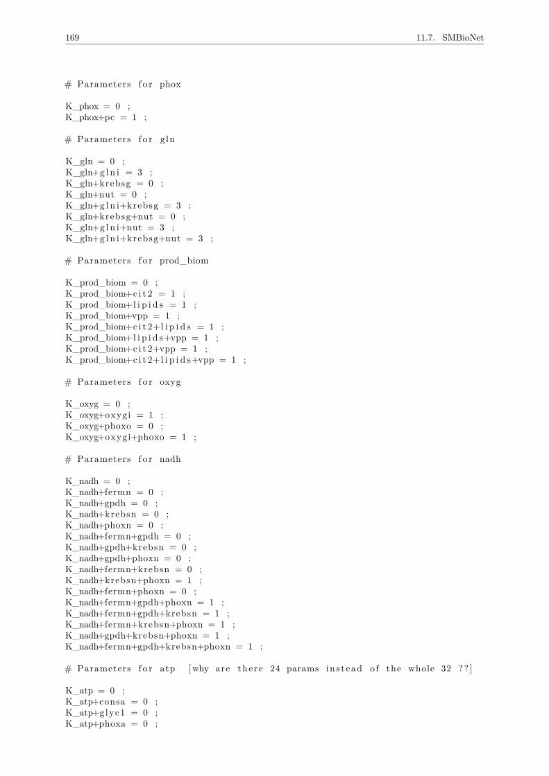
169 11.7. SMBioNet
# Parameters f o r phox
K_phox = 0 ;K_phox+pc = 1 ;
# Parameters f o r g ln
K_gln = 0 ;K_gln+g l n i = 3 ;K_gln+krebsg = 0 ;K_gln+nut = 0 ;K_gln+g l n i+krebsg = 3 ;K_gln+krebsg+nut = 0 ;K_gln+g l n i+nut = 3 ;K_gln+g l n i+krebsg+nut = 3 ;
# Parameters f o r prod_biom
K_prod_biom = 0 ;K_prod_biom+c i t 2 = 1 ;K_prod_biom+l i p i d s = 1 ;K_prod_biom+vpp = 1 ;K_prod_biom+c i t 2+l i p i d s = 1 ;K_prod_biom+l i p i d s+vpp = 1 ;K_prod_biom+c i t 2+vpp = 1 ;K_prod_biom+c i t 2+l i p i d s+vpp = 1 ;
# Parameters f o r oxyg
K_oxyg = 0 ;K_oxyg+oxygi = 1 ;K_oxyg+phoxo = 0 ;K_oxyg+oxygi+phoxo = 1 ;
# Parameters f o r nadh
K_nadh = 0 ;K_nadh+fermn = 0 ;K_nadh+gpdh = 0 ;K_nadh+krebsn = 0 ;K_nadh+phoxn = 0 ;K_nadh+fermn+gpdh = 0 ;K_nadh+gpdh+krebsn = 0 ;K_nadh+gpdh+phoxn = 0 ;K_nadh+fermn+krebsn = 0 ;K_nadh+krebsn+phoxn = 1 ;K_nadh+fermn+phoxn = 0 ;K_nadh+fermn+gpdh+phoxn = 1 ;K_nadh+fermn+gpdh+krebsn = 1 ;K_nadh+fermn+krebsn+phoxn = 1 ;K_nadh+gpdh+krebsn+phoxn = 1 ;K_nadh+fermn+gpdh+krebsn+phoxn = 1 ;
# Parameters f o r atp [why are the re 24 params in s t ead o f the whole 32 ? ? ]
K_atp = 0 ;K_atp+consa = 0 ;K_atp+glyc1 = 0 ;K_atp+phoxa = 0 ;
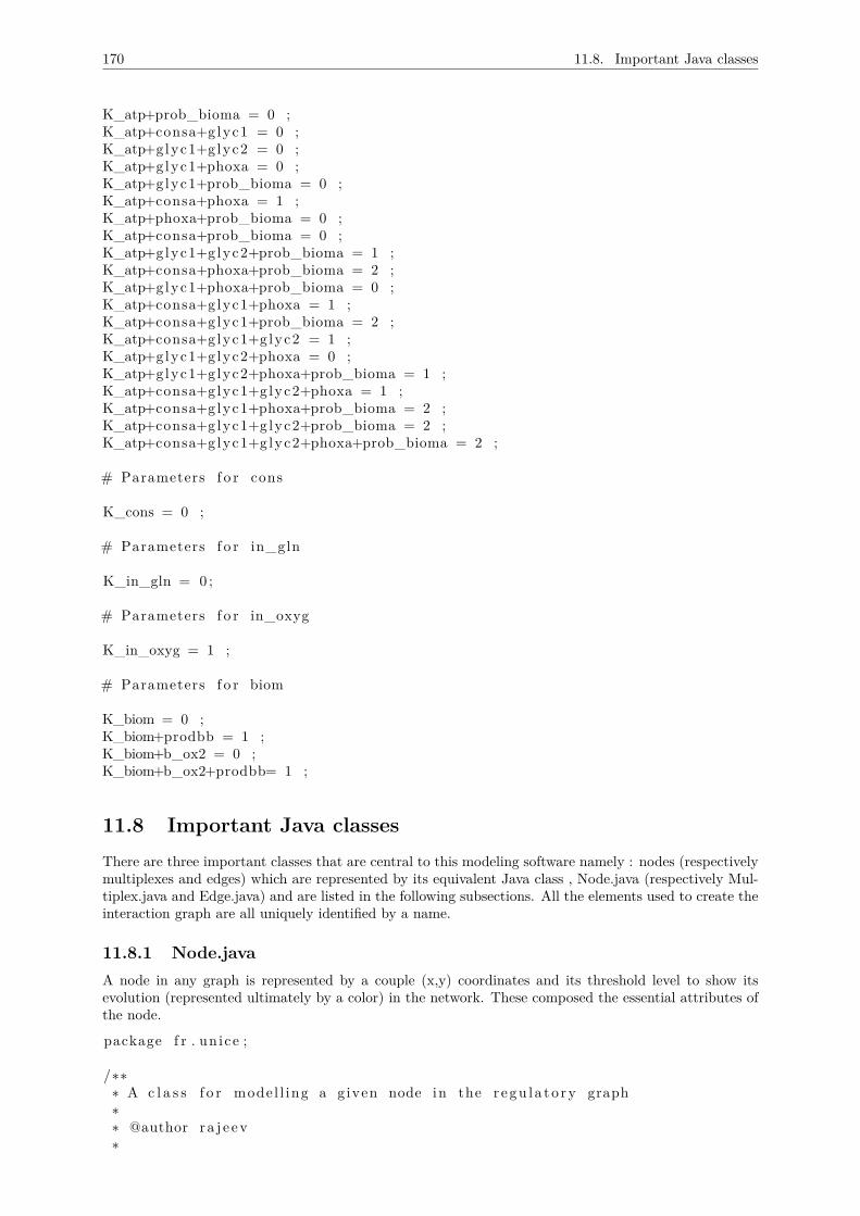
170 11.8. Important Java classes
K_atp+prob_bioma = 0 ;K_atp+consa+glyc1 = 0 ;K_atp+glyc1+glyc2 = 0 ;K_atp+glyc1+phoxa = 0 ;K_atp+glyc1+prob_bioma = 0 ;K_atp+consa+phoxa = 1 ;K_atp+phoxa+prob_bioma = 0 ;K_atp+consa+prob_bioma = 0 ;K_atp+glyc1+glyc2+prob_bioma = 1 ;K_atp+consa+phoxa+prob_bioma = 2 ;K_atp+glyc1+phoxa+prob_bioma = 0 ;K_atp+consa+glyc1+phoxa = 1 ;K_atp+consa+glyc1+prob_bioma = 2 ;K_atp+consa+glyc1+glyc2 = 1 ;K_atp+glyc1+glyc2+phoxa = 0 ;K_atp+glyc1+glyc2+phoxa+prob_bioma = 1 ;K_atp+consa+glyc1+glyc2+phoxa = 1 ;K_atp+consa+glyc1+phoxa+prob_bioma = 2 ;K_atp+consa+glyc1+glyc2+prob_bioma = 2 ;K_atp+consa+glyc1+glyc2+phoxa+prob_bioma = 2 ;
# Parameters f o r cons
K_cons = 0 ;
# Parameters f o r in_gln
K_in_gln = 0 ;
# Parameters f o r in_oxyg
K_in_oxyg = 1 ;
# Parameters f o r biom
K_biom = 0 ;K_biom+prodbb = 1 ;K_biom+b_ox2 = 0 ;K_biom+b_ox2+prodbb= 1 ;
11.8 Important Java classesThere are three important classes that are central to this modeling software namely : nodes (respectivelymultiplexes and edges) which are represented by its equivalent Java class , Node.java (respectively Mul-tiplex.java and Edge.java) and are listed in the following subsections. All the elements used to create theinteraction graph are all uniquely identified by a name.
11.8.1 Node.javaA node in any graph is represented by a couple (x,y) coordinates and its threshold level to show itsevolution (represented ultimately by a color) in the network. These composed the essential attributes ofthe node.
package f r . un ice ;
/∗∗∗ A c l a s s f o r mode l l ing a g iven node in the r egu l a t o ry graph∗∗ @author r a j e ev∗
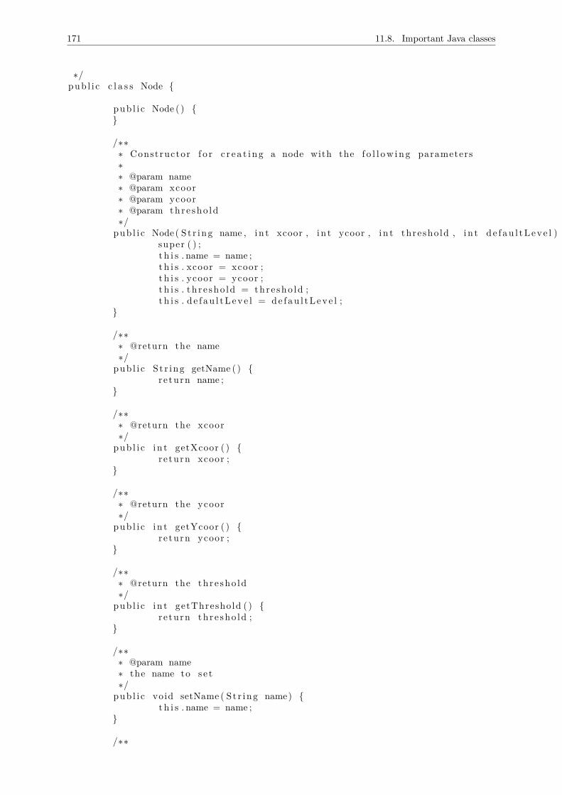
171 11.8. Important Java classes
∗/pub l i c c l a s s Node {
pub l i c Node ( ) {}
/∗∗∗ Constructor f o r c r e a t i n g a node with the f o l l ow i ng parameters∗∗ @param name∗ @param xcoor∗ @param ycoor∗ @param thre sho ld∗/
pub l i c Node ( St r ing name , i n t xcoor , i n t ycoor , i n t thresho ld , i n t d e f au l tLev e l ) {super ( ) ;t h i s . name = name ;t h i s . xcoor = xcoor ;t h i s . ycoor = ycoor ;t h i s . th r e sho ld = thre sho ld ;t h i s . d e f au l tLev e l = de f au l tLev e l ;
}
/∗∗∗ @return the name∗/
pub l i c S t r ing getName ( ) {re turn name ;
}
/∗∗∗ @return the xcoor∗/
pub l i c i n t getXcoor ( ) {re turn xcoor ;
}
/∗∗∗ @return the ycoor∗/
pub l i c i n t getYcoor ( ) {re turn ycoor ;
}
/∗∗∗ @return the th r e sho ld∗/
pub l i c i n t getThreshold ( ) {re turn thr e sho ld ;
}
/∗∗∗ @param name∗ the name to s e t∗/
pub l i c void setName ( St r ing name) {t h i s . name = name ;
}
/∗∗
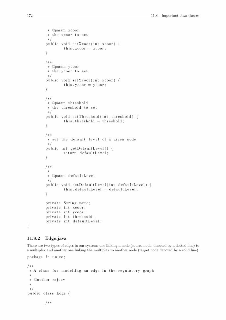
172 11.8. Important Java classes
∗ @param xcoor∗ the xcoor to s e t∗/
pub l i c void setXcoor ( i n t xcoor ) {t h i s . xcoor = xcoor ;
}
/∗∗∗ @param ycoor∗ the ycoor to s e t∗/
pub l i c void setYcoor ( i n t ycoor ) {t h i s . ycoor = ycoor ;
}
/∗∗∗ @param thre sho ld∗ the th r e sho ld to s e t∗/
pub l i c void setThresho ld ( i n t th r e sho ld ) {t h i s . th r e sho ld = thre sho ld ;
}
/∗∗∗ s e t the d e f au l t l e v e l o f a g iven node∗/
pub l i c i n t ge tDe fau l tLeve l ( ) {re turn de f au l tL ev e l ;
}
/∗∗∗∗ @param de f au l tLev e l∗/
pub l i c void s e tDe f au l tLeve l ( i n t d e f au l tLev e l ) {t h i s . d e f au l tLev e l = de f au l tLev e l ;
}
p r i va t e St r ing name ;p r i va t e i n t xcoor ;p r i va t e i n t ycoor ;p r i va t e i n t th r e sho ld ;p r i va t e i n t d e f au l tL ev e l ;
}
11.8.2 Edge.javaThere are two types of edges in our system: one linking a node (source node, denoted by a dotted line) toa multiplex and another one linking the multiplex to another node (target node denoted by a solid line).
package f r . un ice ;
/∗∗∗ A c l a s s f o r mode l l ing an edge in the r egu l a t o ry graph∗∗ @author r a j e ev∗∗/
pub l i c c l a s s Edge {
/∗∗
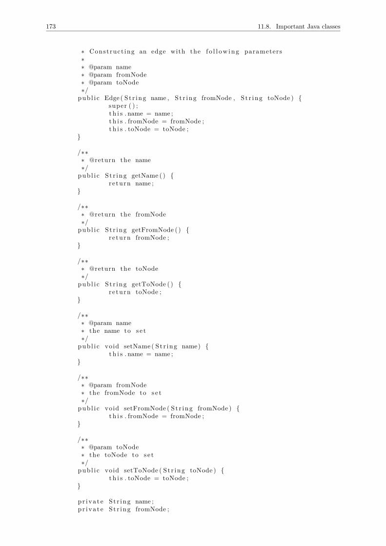
173 11.8. Important Java classes
∗ Construct ing an edge with the f o l l ow i ng parameters∗∗ @param name∗ @param fromNode∗ @param toNode∗/
pub l i c Edge ( S t r ing name , S t r ing fromNode , S t r ing toNode ) {super ( ) ;t h i s . name = name ;t h i s . fromNode = fromNode ;t h i s . toNode = toNode ;
}
/∗∗∗ @return the name∗/
pub l i c S t r ing getName ( ) {re turn name ;
}
/∗∗∗ @return the fromNode∗/
pub l i c S t r ing getFromNode ( ) {re turn fromNode ;
}
/∗∗∗ @return the toNode∗/
pub l i c S t r ing getToNode ( ) {re turn toNode ;
}
/∗∗∗ @param name∗ the name to s e t∗/
pub l i c void setName ( St r ing name) {t h i s . name = name ;
}
/∗∗∗ @param fromNode∗ the fromNode to s e t∗/
pub l i c void setFromNode ( St r ing fromNode ) {t h i s . fromNode = fromNode ;
}
/∗∗∗ @param toNode∗ the toNode to s e t∗/
pub l i c void setToNode ( St r ing toNode ) {t h i s . toNode = toNode ;
}
p r i va t e S t r ing name ;p r i va t e S t r ing fromNode ;
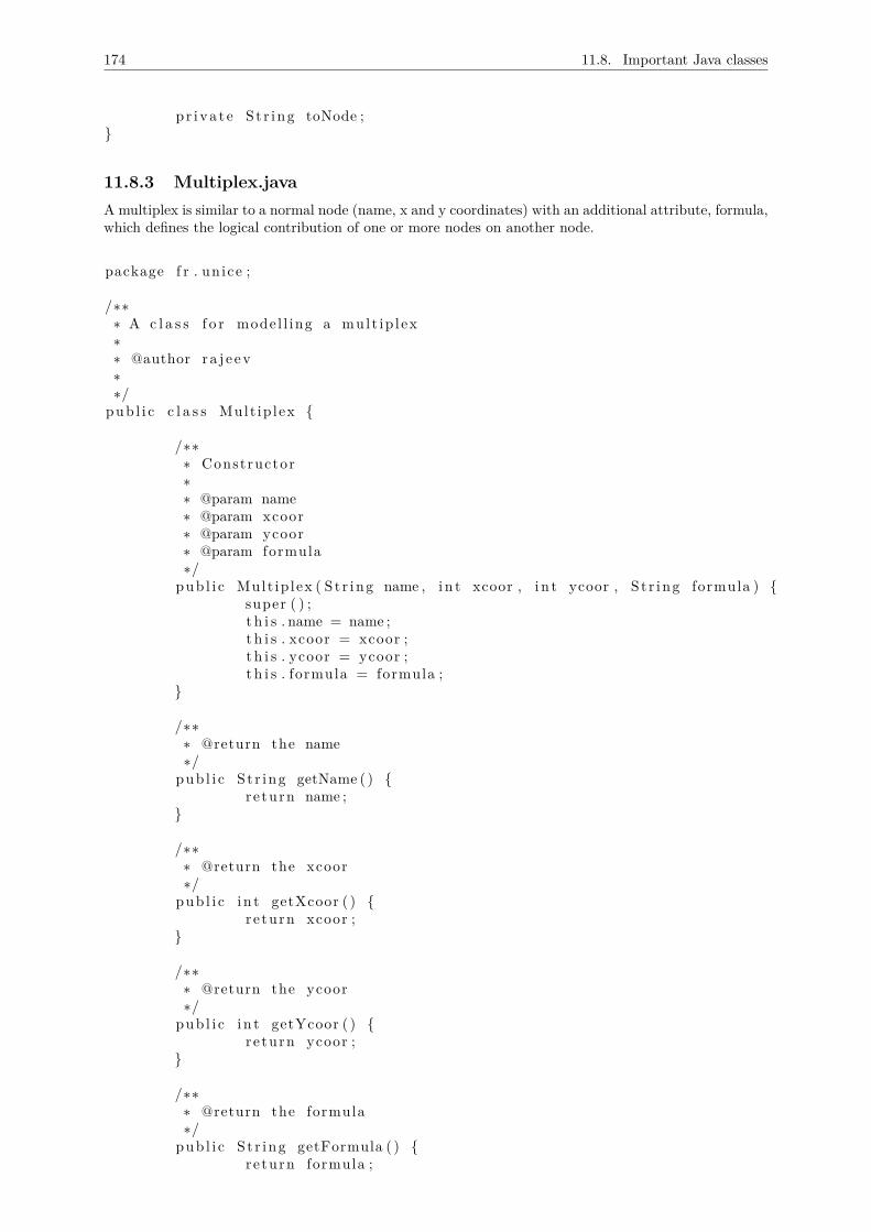
174 11.8. Important Java classes
p r i va t e St r ing toNode ;}
11.8.3 Multiplex.javaA multiplex is similar to a normal node (name, x and y coordinates) with an additional attribute, formula,which defines the logical contribution of one or more nodes on another node.
package f r . un ice ;
/∗∗∗ A c l a s s f o r mode l l ing a mul t ip l ex∗∗ @author r a j e ev∗∗/
pub l i c c l a s s Mult ip lex {
/∗∗∗ Constructor∗∗ @param name∗ @param xcoor∗ @param ycoor∗ @param formula∗/
pub l i c Mult ip lex ( S t r ing name , i n t xcoor , i n t ycoor , S t r ing formula ) {super ( ) ;t h i s . name = name ;t h i s . xcoor = xcoor ;t h i s . ycoor = ycoor ;t h i s . formula = formula ;
}
/∗∗∗ @return the name∗/
pub l i c S t r ing getName ( ) {re turn name ;
}
/∗∗∗ @return the xcoor∗/
pub l i c i n t getXcoor ( ) {re turn xcoor ;
}
/∗∗∗ @return the ycoor∗/
pub l i c i n t getYcoor ( ) {re turn ycoor ;
}
/∗∗∗ @return the formula∗/
pub l i c S t r ing getFormula ( ) {re turn formula ;
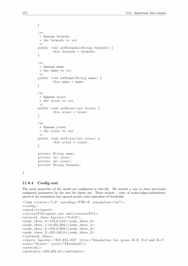
175 11.8. Important Java classes
}
/∗∗∗ @param formula∗ the formula to s e t∗/
pub l i c void setFormula ( S t r ing formula ) {t h i s . formula = formula ;
}
/∗∗∗ @param name∗ the name to s e t∗/
pub l i c void setName ( St r ing name) {t h i s . name = name ;
}
/∗∗∗ @param xcoor∗ the xcoor to s e t∗/
pub l i c void setXcoor ( i n t xcoor ) {t h i s . xcoor = xcoor ;
}
/∗∗∗ @param ycoor∗ the ycoor to s e t∗/
pub l i c void setYcoor ( i n t ycoor ) {t h i s . ycoor = ycoor ;
}
p r i va t e St r ing name ;p r i va t e i n t xcoor ;p r i va t e i n t ycoor ;p r i va t e St r ing formula ;
}
11.8.4 Config.xmlThe main properties of the model are configured in this file. We needed a way to store previouslyconfigured parameters by the user for future use. These include : color of nodes/edges/multiplexes,speed of the simulation, last opened model, color equivalent of thresholds.
<?xml ve r s i on ="1.0" encoding="UTF−8" s tanda lone="no"?><conf ig><speed>1</speed><cur r en tF i l e >genes_xyz . xml</cur r en tF i l e ><network_thres bgco lo r ="0 ,0 ,0"><node_thres_0 >153 ,0 ,153</node_thres_0><node_thres_1 >0 ,255 ,204</node_thres_1><node_thres_2 >255 ,0 ,204</node_thres_2><node_thres_3 >255 ,102 ,0</node_thres_3></network_thres><char t s bgco lo r ="255 ,255 ,255" t i t l e ="Simulat ion f o r genes X=0, Y=1 and Z=1"xax i s="Sta t e s " yax i s="Threshold "/><network/><mult ip lex >204 ,255 ,51</mult ip lex>
176 11.8. Important Java classes
<dottedEdge >204 ,0 ,255</dottedEdge><normalEdge >255 ,102 ,102</normalEdge></con f ig>
11.8.5 Config.javaThe Config.java file acts as an interface between the Config.xml file and the metabolic model.
11.8.6 Network.javaThe core methods of DyMBioNet are centralized in this class. All interactions (CRUD actions) betweenthe user and the software are implemented in this java class.
L i s t o f methods
void addCTL( java . lang . S t r ing c t l )This method w i l l add a new CTL or update the e x i s t i n g CTL f o r a g iven model
i n t addEdge ( i n t mode , java . lang . S t r ing edgeName , java . lang . S t r ing fromNode ,java . lang . S t r ing toNode )THis method enab l e s the user to add an edge in the graph
void addModelFromSMBioNet ( java . lang . S t r ing fi leName , java . u t i l . ArrayList<Node> nodeArr )THis method w i l l be used when user wants to run model ( s ) generated fromSMBioNet ( v a l i d a t i n g a c e r t a i n CTL formula )
boolean addMultiplex ( java . lang . S t r ing multName , java . lang . S t r ing formula ,java . lang . S t r ing xcoor , java . lang . S t r ing ycoor )This method a l l ows the user to add a mul t ip l ex with the f o l l ow i ng parameters :
boolean addNode ( java . lang . S t r ing nodeName , java . lang . S t r ing xCoor , java . lang . S t r ingyCoor , java . lang . S t r ing th r e sho ld )
This method i s used to add a node to your network f i l e with the f o l l ow i ng parameters :
void addParameter ( java . lang . S t r ing nodeId , java . lang . S t r ing rowCol , i n t de fau l tValue ,boolean isEnd )
This method i s used to add K parameter from Kinet i c window to xml f i l e
boolean convertToSmBioNet ( )This method i s used to generate SmBioNet from DymBioNet xml f i l e
void generateModelFromSmBioNet ( java . lang . S t r ing f i l ename , java . i o . F i l e f )Generate model from SmBionet f i l e
void generateNetwork ( java . lang . S t r ing fi leName , java . lang . S t r ing f i l eD e s c )This method i s used to generate xml f i l e from c l a s s i c SymBionet f i l e
java . lang . S t r ing getCTL ( )This method w i l l r e turn CTL formula f o r t h i s model
i n t [ ] getDefaultParamsOfNodes (Node [ ] nodes )This method r e t r i e v e s the d e f au l t parameters f o r each node . . . . s imu la t i on
Edge [ ] getEdges ( )This method i s used to get l i s t o f edges from a given xml f i l e / network
Mult ip lex [ ] g e tMul t ip l exe s ( )This method w i l l output the l i s t o f mu l t i p l exe s from the graph
177 11.8. Important Java classes
Mult ip lex getMultiplexInfoByName ( java . lang . S t r ing multName)Get a l l in fo rmat ion on a mul t ip l ex by i t s name
Node getNodeInfoByName ( java . lang . S t r ing nodeName)Get a l l in fo rmat ion on a node by i t s name in the graph
Mult ip lex [ ] getPosMults ( boolean p o s i t i v e )This w i l l r e turn the l i s t o f a c t i v a t i o n s
i n t ge tS ta r tMu l t ip l ex ( )This method i s c a l l e d from too lba r when c r e a t i n g a mul t ip l ex
void r eadF i l e ( java . lang . S t r ing f i leName )THis method i s used to i n i t i a l i s e a model f o r read ing
void removeEdge ( java . lang . S t r ing edgeName)This method i s used to remove an edge
void s av eF i l e ( java . lang . S t r ing f i leName )This method i s c a l l e d each time a network i s created , a node , edge ormul t ip l ex i s added
void updateFromSMBioNet ( i n t modelNo , java . u t i l . ArrayList<java . lang . Str ing>arrNodes , java . u t i l .Map<java . lang . Str ing , java . lang . Integer> valNodes )
Update xml f i l e based on the model chosen by the user from ’Launch SMBioNet ’window
void updateKParameters ( java . lang . S t r ing nodeName , i n t row , i n t co l ,java . lang . S t r ing newValue )This method w i l l be c a l l e d when user mod i f i e s K Parameter in Kinet i c t ab l e
void updateMultiplexFormula ( boolean checked )This method w i l l change whether mul t ip l ex formula mustbe shown or not
boolean updateNodeParams ( org . graphstream . graph . Graph g , java . lang . S t r ingnodeType , java . lang . S t r ing nodeName , java . lang . S t r ing [ ] newValues )This method i s used to update parameters f o r a node or mul t ip l ex in the xml f i l e
void updateNodePos ( i n t nodeType , java . lang . S t r ing nodeName , i n t x , i n t y )This method w i l l be used to update cur rent p o s i t i o n o f a g iven node/mul t ip l ex
11.8.7 Metabolism.xmlThe final version of the metabolic model in the XML format.
<?xml ve r s i on ="1.0" encoding="UTF−8" s tanda lone="no"?><network><des c r i p t i on>Metabol ic network</de s c r i p t i on><nodes><node d e f au l t ="0" id="ATP_ADP" kparam="1" th r e s ="2" weight="1" xcoor="−50" ycoor="100">ATP_ADP<K id="KATP_ADP00000" value="0"/><K id="KATP_ADP00001" value="0"/><K id="KATP_ADP00010" value="0"/><K id="KATP_ADP00011" value="0"/><K id="KATP_ADP00100" value="0"/><K id="KATP_ADP00101" value="0"/><K id="KATP_ADP00110" value="0"/><K id="KATP_ADP00111" value="0"/><K id="KATP_ADP01000" value="0"/><K id="KATP_ADP01001" value="0"/><K id="KATP_ADP01010" value="0"/>
178 11.8. Important Java classes
<K id="KATP_ADP01011" value="0"/><K id="KATP_ADP01100" value="1"/><K id="KATP_ADP01101" value="1"/><K id="KATP_ADP01110" value="2"/><K id="KATP_ADP01111" value="2"/><K id="KATP_ADP10000" value="0"/><K id="KATP_ADP10001" value="0"/><K id="KATP_ADP10010" value="0"/><K id="KATP_ADP10011" value="1"/><K id="KATP_ADP10100" value="0"/><K id="KATP_ADP10101" value="0"/><K id="KATP_ADP10110" value="0"/><K id="KATP_ADP10111" value="1"/><K id="KATP_ADP11000" value="0"/><K id="KATP_ADP11001" value="1"/><K id="KATP_ADP11010" value="2"/><K id="KATP_ADP11011" value="2"/><K id="KATP_ADP11100" value="1"/><K id="KATP_ADP11101" value="1"/><K id="KATP_ADP11110" value="2"/><K id="KATP_ADP11111" value="2"/></node><node de f au l t ="0" id="OXYG" kparam="1" th r e s ="1" weight="1" xcoor="−50" ycoor="−100">OXYG<K id="KOXYG00" value="0"/><K id="KOXYG01" value="0"/><K id="KOXYG10" value="1"/><K id="KOXYG11" value="1"/></node><node de f au l t ="0" id="GLYC" kparam="1" th r e s ="2" weight="1" xcoor ="60" ycoor="90">GLYC<K id="KGLYC0000" va lue="0"/><K id="KGLYC0001" va lue="0"/><K id="KGLYC0010" va lue="0"/><K id="KGLYC0011" va lue="0"/><K id="KGLYC0100" va lue="0"/><K id="KGLYC0101" va lue="0"/><K id="KGLYC0110" va lue="0"/><K id="KGLYC0111" va lue="0"/><K id="KGLYC1000" va lue="0"/><K id="KGLYC1001" va lue="0"/><K id="KGLYC1010" va lue="1"/><K id="KGLYC1011" va lue="1"/><K id="KGLYC1100" va lue="0"/><K id="KGLYC1101" va lue="0"/><K id="KGLYC1110" va lue="1"/><K id="KGLYC1111" va lue="2"/></node><node de f au l t ="2" id="GLU" kparam="1" th r e s ="2" weight="1" xcoor ="50" ycoor="190">GLU<K id="KGLU" value="2"/></node><node de f au l t ="0" id="BIOM" kparam="1" th r e s ="1" weight="1" xcoor ="127" ycoor="95">BIOM<K id="KBIOM00" value="0"/><K id="KBIOM01" value="1"/><K id="KBIOM10" value="0"/><K id="KBIOM11" value="1"/></node><node de f au l t ="0" id="PROD_BIOM" kparam="1" th r e s ="1" weight="1" xcoor ="200"ycoor="140">PROD_BIOM<K id="KPROD_BIOM000" value="0"/><K id="KPROD_BIOM001" value="1"/><K id="KPROD_BIOM010" value="1"/>
179 11.8. Important Java classes
<K id="KPROD_BIOM011" value="1"/><K id="KPROD_BIOM100" value="1"/><K id="KPROD_BIOM101" value="1"/><K id="KPROD_BIOM110" value="1"/><K id="KPROD_BIOM111" value="1"/></node><node de f au l t ="0" id="GLN" kparam="1" th r e s ="3" weight="1" xcoor ="316" ycoor="131">GLN<K id="KGLN000" va lue="0"/><K id="KGLN001" va lue="0"/><K id="KGLN010" va lue="0"/><K id="KGLN011" va lue="0"/><K id="KGLN100" va lue="3"/><K id="KGLN101" va lue="3"/><K id="KGLN110" va lue="3"/><K id="KGLN111" va lue="3"/></node><node de f au l t ="0" id="FERM" kparam="1" th r e s ="1" weight="1" xcoor ="170" ycoor="−5">FERM<K id="KFERM0" value="0"/><K id="KFERM1" value="1"/></node><node de f au l t ="0" id="NADH" kparam="1" th r e s ="3" weight="1" xcoor ="300"ycoor="−10">NADH<K id="KNADH0000" va lue="0"/><K id="KNADH0001" va lue="0"/><K id="KNADH0010" va lue="0"/><K id="KNADH0011" va lue="1"/><K id="KNADH0100" va lue="0"/><K id="KNADH0101" va lue="0"/><K id="KNADH0110" va lue="0"/><K id="KNADH0111" va lue="1"/><K id="KNADH1000" va lue="0"/><K id="KNADH1001" va lue="0"/><K id="KNADH1010" va lue="0"/><K id="KNADH1011" va lue="1"/><K id="KNADH1100" va lue="0"/><K id="KNADH1101" va lue="1"/><K id="KNADH1110" va lue="1"/><K id="KNADH1111" va lue="1"/></node><node de f au l t ="0" id="KREBS" kparam="1" th r e s ="2" weight="1" xcoor ="110"ycoor="−70">KREBS<K id="KKREBS000" va lue="0"/><K id="KKREBS001" value="0"/><K id="KKREBS010" value="1"/><K id="KKREBS011" value="0"/><K id="KKREBS100" value="1"/><K id="KKREBS101" value="2"/><K id="KKREBS110" value="0"/><K id="KKREBS111" value="0"/></node><node de f au l t ="0" id="PHOX" kparam="1" th r e s ="1" weight="1" xcoor ="100"ycoor="−180">PHOX<K id="KPHOX0" value="0"/><K id="KPHOX1" value="1"/></node><node de f au l t ="0" id="CONS" kparam="1" th r e s ="1" weight="1" xcoor="−100"ycoor="200">CONS<K id="KCONS" value="0"/></node><node de f au l t ="0" id="IN_GLN" kparam="1" th r e s ="1" weight="1" xcoor ="450"ycoor="190">IN_GLN<K id="KIN_GLN" value="0"/></node><node de f au l t ="1" id="IN_OXYG" kparam="1" th r e s ="1" weight="1" xcoor="−130"
180 11.8. Important Java classes
ycoor="−180">IN_OXYG<K id="KIN_OXYG" value="1"/></node>
</nodes><edges><edge fromNode="GLYC1" id="e38 " toNode="ATP_ADP">e38</edge><edge fromNode="CONSA" id="e39 " toNode="ATP_ADP">e39</edge><edge fromNode="PHOXA" id="e54 " toNode="ATP_ADP">e54</edge><edge fromNode="PROD_BIOMA" id="e55 " toNode="ATP_ADP">e55</edge><edge fromNode="GLYC2" id="e65 " toNode="ATP_ADP">e65</edge><edge fromNode="NAD+" id="e2 " toNode="GLYC">e2</edge><edge fromNode="CIT" id="e13 " toNode="GLYC">e13</edge><edge fromNode="GLU1" id="e42 " toNode="GLYC">e42</edge><edge fromNode="GLU2" id="e43 " toNode="GLYC">e43</edge><edge fromNode="GPDH" id="e15 " toNode="NADH">e15</edge><edge fromNode="FERMN" id="e50 " toNode="NADH">e50</edge><edge fromNode="KREBSN" id="e51 " toNode="NADH">e51</edge><edge fromNode="PHOXN" id="e53 " toNode="NADH">e53</edge><edge fromNode="OXYGI" id="e40 " toNode="OXYG">e40</edge><edge fromNode="PHOXO" id="e41 " toNode="OXYG">e41</edge><edge fromNode="GLNI" id="e47 " toNode="GLN">e47</edge><edge fromNode="GLN−NUT" id="e48 " toNode="GLN">e48</edge><edge fromNode="KREBSG" id="e49 " toNode="GLN">e49</edge><edge fromNode="EX−PYR" id="e28 " toNode="FERM">e28</edge><edge fromNode="PC" id="e24 " toNode="PHOX">e24</edge><edge fromNode="B−OX" id="e31 " toNode="KREBS">e31</edge><edge fromNode="SAT" id="e32 " toNode="KREBS">e32</edge><edge fromNode="PYR" id="e4 " toNode="KREBS">e4</edge><edge fromNode="VPP" id="e6 " toNode="PROD_BIOM">e6</edge><edge fromNode="LIPIDS " id="e44 " toNode="PROD_BIOM">e44</edge><edge fromNode="CIT2" id="e67 " toNode="PROD_BIOM">e67</edge><edge fromNode="PRODBB" id="e46 " toNode="BIOM">e46</edge><edge fromNode="B−OX" id="e36 " toNode="BIOM">e36</edge><edge fromNode="GLU" id="e7 " toNode="GLU1">e7</edge><edge fromNode="GLU" id="e37 " toNode="GLU2">e37</edge><edge fromNode="ATP_ADP" id="e1 " toNode="NAD+">e1</edge><edge fromNode="ATP_ADP" id="e33 " toNode="B−OX">e33</edge><edge fromNode="ATP_ADP" id="e57 " toNode="VPP">e57</edge><edge fromNode="ATP_ADP" id="e58 " toNode="LIPIDS">e58</edge><edge fromNode="ATP_ADP" id="e62 " toNode="PC">e62</edge><edge fromNode="GLYC" id="e3 " toNode="PYR">e3</edge><edge fromNode="GLYC" id="e9 " toNode="GLYC1">e9</edge><edge fromNode="GLYC" id="e14 " toNode="GPDH">e14</edge><edge fromNode="GLYC" id="e19 " toNode="EX−PYR">e19</edge><edge fromNode="GLYC" id="e22 " toNode="SAT">e22</edge><edge fromNode="GLYC" id="e35 " toNode="B−OX">e35</edge><edge fromNode="GLYC" id="e64 " toNode="GLYC2">e64</edge><edge fromNode="GLYC" id="e69 " toNode="VPP">e69</edge><edge fromNode="PHOX" id="e52 " toNode="PHOXN">e52</edge><edge fromNode="PHOX" id="e56 " toNode="PHOXA">e56</edge><edge fromNode="PHOX" id="e25 " toNode="PHOXO">e25</edge><edge fromNode="IN_GLN" id="e18 " toNode="GLNI">e18</edge><edge fromNode="IN_OXYG" id="e11 " toNode="OXYGI">e11</edge><edge fromNode="CONS" id="e10 " toNode="CONSA">e10</edge><edge fromNode="KREBS" id="e12 " toNode="CIT">e12</edge><edge fromNode="KREBS" id="e29 " toNode="KREBSN">e29</edge><edge fromNode="KREBS" id="e30 " toNode="KREBSG">e30</edge><edge fromNode="KREBS" id="e45 " toNode="CIT2">e45</edge><edge fromNode="FERM" id="e16 " toNode="FERMN">e16</edge>
181 11.8. Important Java classes
<edge fromNode="BIOM" id="e34 " toNode="B−OX">e34</edge><edge fromNode="OXYG" id="e8 " toNode="PYR">e8</edge><edge fromNode="OXYG" id="e21 " toNode="SAT">e21</edge><edge fromNode="OXYG" id="e27 " toNode="EX−PYR">e27</edge><edge fromNode="OXYG" id="e70 " toNode="PC">e70</edge><edge fromNode="PROD_BIOM" id="e5 " toNode="PRODBB">e5</edge><edge fromNode="PROD_BIOM" id="e17 " toNode="GLN−NUT">e17</edge><edge fromNode="PROD_BIOM" id="e60 " toNode="PROD_BIOMA">e60</edge><edge fromNode="PROD_BIOM" id="e66 " toNode="CIT2">e66</edge><edge fromNode="PROD_BIOM" id="e68 " toNode="CIT">e68</edge><edge fromNode="NADH" id="e20 " toNode="PC">e20</edge><edge fromNode="NADH" id="e63 " toNode="NAD+">e63</edge><edge fromNode="NADH" id="e26 " toNode="EX−PYR">e26</edge><edge fromNode="GLN" id="e23 " toNode="SAT">e23</edge><edge fromNode="GLN" id="e59 " toNode="LIPIDS">e59</edge><edge fromNode="GLN" id="e61 " toNode="VPP">e61</edge></edges><mults><mult formula ="! (CONS > ;=1)" id="CONSA" xcoor="−100" ycoor="150">CONSA</mult><mult formula ="! (PROD_BIOM > ;=1)" id="PROD_BIOMA" xcoor ="100"ycoor="200">PROD_BIOMA</mult><mult formula="(GLYC > ;=2)" id="GLYC2" xcoor="0" ycoor="120">GLYC2</mult><mult formula="(GLYC > ;=1)" id="GLYC1" xcoor="0" ycoor="90">GLYC1</mult><mult formula="(PHOX > ; 1 ) " id="PHOXA" xcoor="−140" ycoor="−90">PHOXA</mult><mult formula="(GLU > ;=2)" id="GLU2" xcoor ="80" ycoor="150">GLU2</mult><mult formula="(GLU > ;=1)" id="GLU1" xcoor ="20" ycoor="150">GLU1</mult><mult formula ="! (ATP_ADP > ;=2) & ; ! (NADH > ;=1)" id="NAD+" xcoor="−20"ycoor="60">NAD+</mult><mult formula =" ! ( (KREBS > ;=2) & ; ! (PROD_BIOM > ;=1)) " id="CIT"xcoor ="100" ycoor="0">CIT</mult><mult formula="(IN_OXYG > ;=1)" id="OXYGI" xcoor="−80" ycoor="−145">OXYGI</mult><mult formula ="! (PHOX > ;=1)" id="PHOXO" xcoor ="30" ycoor="−130">PHOXO</mult><mult formula="(IN_GLN > ;=1)" id="GLNI" xcoor ="390" ycoor="186">GLNI</mult><mult formula ="! (PROD_BIOM > ;=1)" id="GLN−NUT" xcoor ="255" ycoor="140">GLN−NUT</mult><mult formula ="! (KREBS > ;=2)" id="KREBSG" xcoor ="388" ycoor="−47">KREBSG</mult><mult formula="(GLYC > ;=1)" id="GPDH" xcoor ="250" ycoor="40">GPDH</mult><mult formula="(KREBS > ;=1)" id="KREBSN" xcoor ="236" ycoor="−88">KREBSN</mult><mult formula ="! (PHOX > ;=1)" id="PHOXN" xcoor ="250" ycoor="−186">PHOXN</mult><mult formula ="! (FERM > ;=1)" id="FERMN" xcoor ="264" ycoor="−2">FERMN</mult><mult formula="(GLYC > ;=1) & ; (OXYG > ;=1)" id="PYR" xcoor="−70"ycoor="0">PYR</mult><mult formula="(BIOM > ;=1) & ; ! (GLYC > ;=1) & ; ! (ATP_ADP > ;=1)"id="B−OX" xcoor="−30" ycoor="−50">B−OX</mult><mult formula ="(((GLYC > ;=1) & ; (GLN > ;=2)) | (GLYC > ;=2)) & ;(OXYG > ;= 1) " id="SAT" xcoor ="40" ycoor="−100">SAT</mult><mult formula="(GLYC > ;=1) & ; (ATP_ADP > ;=1) & ; (GLN > ;=1)"id="VPP" xcoor ="180" ycoor="200">VPP</mult>
<mult formula="(GLN > ;=3) & ; (ATP_ADP > ;=1)" id="LIPIDS " xcoor ="250"ycoor="200">LIPIDS</mult><mult formula ="((KREBS > ;=2) & ; ! (PROD_BIOM > ;=1)) " id="CIT2" xcoor ="100"ycoor="0">CIT2</mult><mult formula ="(((GLYC > ;=1) & ; ! (OXYG > ;=1)) | (GLYC > ;=2)) & ;(NADH > ;=1)" id="EX−PYR" xcoor ="110" ycoor="50">EX−PYR</mult><mult formula="(NADH > ;=1) & ; (OXYG > ;=1) & ; ! (ATP_ADP > ;= 2) "id="PC" xcoor ="210" ycoor="−140">PC</mult><mult formula="(PROD_BIOM > ;=1)" id="PRODBB" xcoor ="160"ycoor="130">PRODBB</mult><mult formula =" ! ( (BIOM > ;=1) & ; ! (GLYC > ;=1) & ; ! (ATP_ADP > ;=1)) "id="BOXB" xcoor ="160" ycoor="130">BOXB</mult>

182 11.8. Important Java classes
</mults><trans >... </ trans></network>
Bibliography
[1] Sebastian Kmiecik, Dominik Gront, Michal Kolinski, Lukasz Wieteska, Aleksandra Elz-bieta Dawid, and Andrzej Kolinski; Chemical Reviews 2016 116 (14), 7898-7936; DOI:10.1021/acs.chemrev.6b00163
[2] Bernot G, Comet JP, Richard A, Guespin J. Application of formal methods to biological regulatorynetworks: extending Thomas’ asynchronous logical approach with temporal logic. J Theor Biol.2004;229(3):339-347; DOI:10.1016/j.jtbi.2004.04.003
[3] Bernot, G., Comet, J. P., Khalis, Z., Richard, A., & Roux, O. (2019). A genetically modified Hoarelogic. Theoretical Computer Science, 765, 145-157.
[4] Lunt SY, Vander Heiden MG. Aerobic glycolysis: meeting the metabolic requirements of cell pro-liferation. Annu Rev Cell Dev Biol. 2011;27:441-64; DOI: 10.1146/annurev-cellbio-092910-154237.PMID: 21985671
[5] DeBerardinis RJ, Chandel NS. Fundamentals of cancer metabolism. Sci Adv. 2016 May27;2(5):e1600200; DOI: 10.1126/sciadv.1600200. PMID: 27386546; PMCID: PMC4928883
[6] Newsholme EA, Crabtree B, Ardawi MS. Glutamine metabolism in lymphocytes: its biochemical,physiological and clinical importance. Q J Exp Physiol. 1985 Oct;70(4):473-89; DOI: 10.1113/exp-physiol.1985.sp002935. PMID: 3909197
[7] Kovacevic, Z., and McGivan, J.D. (1983). Mitochondrial metabolism of glutamine and glutamateand its physiological significance. Physiol. Rev.63,547-605.
[8] Kerkhoven EJ, Achcar F, Alibu VP, Burchmore RJ, Gilbert IH, et al. (2013) Handling Uncertaintyin Dynamic Models: The Pentose Phosphate Pathway in Trypanosoma brucei. PLoS Comput Biol9(12): e1003371; DOI:10.1371/journal.pcbi.1003371
[9] Loureiro I, Faria J, Santarem N, Smith TK, Tavares J, Cordeiro-da-Silva A. Potential Drug Targetsin the Pentose Phosphate Pathway of Trypanosomatids. Curr Med Chem. 2018;25(39):5239-5265;DOI:10.2174/0929867325666171206094752
[10] Jiang, P., Du, W. & Wu, M. Regulation of the pentose phosphate pathway in cancer. Protein Cell5, 592-602 (2014); DOI:10.1007/s13238-014-0082-8
[11] Bensaad K, Tsuruta A, Selak MA, Vidal MN, Nakano K, Bartrons R, Gottlieb E, Vousden KH.TIGAR, a p53-inducible regulator of glycolysis and apoptosis. Cell. 2006 Jul 14;126(1):107-20;DOI:10.1016/j.cell.2006.05.036. PMID: 16839880
[12] Jiang, Dadi and Brady, Colleen A. and Johnson, Thomas M. and Lee, Eunice Y. and Park, EuniceJ. and Scott, Matthew P. and Attardi, Laura D; Full p53 transcriptional activation potential is dis-pensable for tumor suppression in diverse lineages; Proceedings of the National Academy of Sciences108 (41) pp. 17123 - 28 (2011); DOI:10.1073/pnas.1111245108
[13] Machné R, Murray DB (2012); The Yin and Yang of Yeast Transcription: Elements of a GlobalFeedback System between Metabolism and Chromatin; [PloS One, 716] p. e37906
[14] Dell’ Antone P. Energy metabolism in cancer cells: how to explain the Warburg and Crabtree effects?Med Hypotheses. 2012 Sep;79(3):388-92; DOI: 10.1016/j.mehy.2012.06.002. Epub 2012 Jul 5. PMID:22770870
[15] Rodrigo Diaz-Ruiz, Michel Rigoulet, Anne Devin; The Warburg and Crabtree effects: On the ori-gin of cancer cell energy metabolism and of yeast glucose repression; Biochim Biophys Acta. 2011Jun;1807(6):568-76; DOI: 10.1016/j.bbabio.2010.08.010. Epub 2010 Sep 8. PMID: 20804724.
[16] Liberti MV, Locasale JW. The Warburg Effect: How Does it Benefit Cancer Cells? Trends BiochemSci. 2016 Mar;41(3):211-218; DOI: 10.1016/ j.tibs.2015.12.001. Epub 2016 Jan 5.
183
184 Bibliography
[17] Paolo Dell’ Antone, Energy metabolism in cancer cells: How to explain the Warburg andCrabtree effects?, Medical Hypotheses,Volume 79, Issue 3,2012, pp. 388-392,ISSN 0306-9877;DOI:10.1016/j.mehy.2012.06.002
[18] Cairns RA. Drivers of the Warburg phenotype. Cancer J. 2015 Mar-Apr; 21(2):56-61; DOI:10.1097/PPO.0000000000000106. PMID: 25815844
[19] Czernin, J., Allen-Auerbach, M., Nathanson, D. et al. PET/CT in Oncology: Current Status andPerspectives. Curr Radiol Rep 1, 177–190 (2013); DOI:10.1007/s40134-013-0016-x
[20] Maria V. Liberti and Jason W. Locasale; The Warburg Effect: How Does it Benefit Cancer Cells? ;Trends Biochem Sci. 2016 March ; 41(3): 211–218; DOI:10.1016/j.tibs.2015.12.001
[21] Liberti MV, Locasale JW. Correction to: The Warburg Effect: How Does it Benefit Cancer Cells? :[Trends in Biochemical Sciences, 41 (2016) 211]; DOI:10.1016/j.tibs.2016.01.004
[22] Zhang JY, Zhang F, Hong CQ, Giuliano AE, Cui XJ, Zhou GJ, Zhang GJ, Cui YK. Critical proteinGAPDH and its regulatory mechanisms in cancer cells. Cancer Biol Med. 2015 Mar;12(1):10-22;DOI: 10.7497/j.issn.2095-3941.2014.0019. PMID: 25859407; PMCID: PMC4383849
[23] George S Krasnov, Alexey A Dmitriev, Anastasiya V Snezhkina & Anna V Kudryavtseva (2013)Deregulation of glycolysis in cancer: glyceraldehyde-3-phosphate dehydrogenase as a therapeutictarget, Expert Opinion on Therapeutic Targets, 17:6, 681-693; DOI: 10.1517/14728222.2013.775253
[24] Tang, Z., Yuan, S., Hu, Y. et al. Over-expression of GAPDH in human colorectal carcinoma as apreferred target of 3-Bromopyruvate Propyl Ester. J Bioenerg Biomembr 44, 117–125 (2012); DOI:10.1007/s10863-012-9420-9
[25] Nguyen TL, Durán RV. Glutamine metabolism in cancer therapy. Cancer Drug Resist 2018;1:126-38;DOI: 10.20517/cdr.2018.08
[26] Bar-Even, A., Flamholz, A., Noor, E. et al. Rethinking glycolysis: on the biochemical logic ofmetabolic pathways. Nat Chem Biol 8, 509–517 (2012); DOI: 10.1038/nchembio.971
[27] Elizabeth L. Lieu, Tu Nguyen, Shawn Rhyne, and Jiyeon Kim; Mol Med. 2020 Jan; 52(1): 15–30;DOI: 10.1038/s12276-020-0375-3; PMCID: PMC7000687
[28] Cristina Bianchi and Maria Luisa Genova and Giovanna Parenti Castelli and Giorgio Lenaz; TheMitochondrial Respiratory Chain Is Partially Organized in a Supercomplex Assembly, Journal ofBiological Chemistry (2004); Vol. 279, No. 35, Issue of August 27, pp. 36562–36569, 2004; DOI:10.1074/jbc.M405135200
[29] Molenaar D, van Berlo R, de Ridder D, Teusink B. Shifts in growth strategies reflect tradeoffs incellular economics. Mol Syst Biol. 2009;5:323; DOI: 10.1038/msb.2009.82. Epub 2009 Nov 3. PMID:19888218; PMCID: PMC2795476
[30] Asha Kumari, Chapter 4 - Beta Oxidation of Fatty Acids, Sweet Biochemistry,Academic Press,2018,pp. 17-19, ISBN 9780128144534; DOI: 10.1016/B978-0-12-814453-4.00004-2
[31] Mondesir J, Willekens C, Touat M, de Botton S. IDH1 and IDH2 mutations as novel therapeutictargets: current perspectives. J Blood Med. 2016 Sep 2;7:171-80; DOI: 10.2147/JBM.S70716. PMID:27621679; PMCID: PMC5015873
[32] Lisa M Lindqvist, Kristofferson Tandoc, Ivan Topisirovic, Luc Furic,Cross-talk between proteinsynthesis, energy metabolism and autophagy in cancer, Current Opinion in Genetics & Develop-ment,Volume 48,2018, pp. 104-111,ISSN 0959-437X; DOI: 10.1016/j.gde.2017.11.003
[33] G, Dr, Naga Rathna Supriya & Prajapati, Bhumi. (2017). Review on Anticancer enzymesand their targeted amino acids. World Journal of Pharmaceutical Research. 2. 268-284; DOI :10.20959/wjpr201712-9676
[34] Anderson, N.M., Mucka, P., Kern, J.G. et al. The emerging role and targetability of the TCA cyclein cancer metabolism. Protein Cell 9, 216–237 (2018); DOI: 10.1007/s13238-017-0451-1
[35] G, Dr, Naga Rathna Supriya & Prajapati, Bhumi. (2017). REVIEW ON ANTICANCER ENZYMESAND THEIR TARGETED AMINO ACIDS. World Journal of Pharmaceutical Research. 2. 268-284;DOI : 10.20959/wjpr201712-9676
185 Bibliography
[36] Migita T, Narita T, Nomura K, Miyagi E, Inazuka F, Matsuura M, Ushijima M, Mashima T, SeimiyaH, Satoh Y, et al. ATP citrate lyase: activation and therapeutic implications in non-small cell lungcancer. Cancer Res. 2008;68 (20) :8547-8554
[37] Jiang, C., Li, X., Zhao, H. et al. Long non-coding RNAs: potential new biomarkers for predictingtumor invasion and metastasis. Mol Cancer 15 (1) pp. 1 - 15, 62 (2016); DOI: 10.1186/s12943-016-0545-z
[38] Jinheng Wang, Yongjiang Zheng, and Meng Zhao; Exosome-Based Cancer Therapy: Implication forTargeting Cancer Stem Cells; Frontiers in Pharmacology, 7, p. 533; DOI: 10.3389/ fphar.2016.00533
[39] Menendez JA, Vellon L, Mehmi I, Oza BP, Ropero S, Colomer R, Lupu R. Inhibition of fatty acidsynthase (FAS) suppresses HER2/neu (erbB-2) oncogene overexpression in cancer cells. Proc NatlAcad Sci U S A. 2004 Jul 20;101(29):10715-20; DOI: 10.1073/pnas.0403390101.
[40] Swinnen JV, Roskams T, Joniau S, Van Poppel H, Oyen R, Baert L, Heyns W, Verhoeven G.Overexpression of fatty acid synthase is an early and common event in the development of prostatecancer. Int J Cancer. 2002 Mar 1;98(1):19-22; DOI: 10.1002/ijc.10127. PMID: 11857379.
[41] Seltzer MJ, Bennett BD, Joshi AD, Gao P, Thomas AG, Ferraris DV, Tsukamoto T, RojasCJ, Slusher BS, Rabinowitz JD, Dang CV, Riggins GJ. Inhibition of glutaminase preferentiallyslows growth of glioma cells with mutant IDH1. Cancer Res. 2010 Nov 15;70(22):8981-7; DOI:10.1158/0008-5472.CAN-10-1666. Epub 2010 Nov 2. PMID: 21045145; PMCID: PMC3058858
[42] Cheng J, Xu J, Duanmu J, Zhou H, Booth CJ, Hu Z. Effective treatment of human lung cancer bytargeting tissue factor with a factor VII-targeted photodynamic therapy. Curr Cancer Drug Targets.2011 Nov;11(9):1069-81; DOI: 10.2174/156800911798073023. PMID: 21933104.
[43] Oettgen HF, Old LJ, Boyse EA, Campbell HA, Philips FS, Clarkson BD, Tallal L, Leeper RD,Schwartz MK, Kim JH. Inhibition of leukemias in man by L-asparaginase. Cancer Res. 1967Dec;27(12):2619-31. PMID: 5237354.
[44] Lo M, Wang YZ, Gout PW. The x(c)- cystine/glutamate antiporter: a potential target for therapy ofcancer and other diseases. J Cell Physiol. 2008 Jun;215(3):593-602; DOI: 10.1002/jcp.21366. PMID:18181196.
[45] Rodman S. N., Spence J. M., Ronnfeldt T. J., Zhu Y., Solst S. R., ONeill R. A., et al. (2016).Enhancement of radiation response in breast cancer stem cells by inhibition of thioredoxin andglutathione-dependent metabolism. Radiat. Res. 186 385-39; DOI: 10.1667/RR14463.1
[46] Sajnani K, Islam F, Smith RA, Gopalan V, Lam AK. Genetic alterations in Krebs cycle and its impacton cancer pathogenesis. Biochimie. 2017 Apr;135:164-172; DOI: 10.1016/j.biochi.2017.02.008. Epub2017 Feb 20. PMID: 28219702
[47] Berg JM, Tymoczko JL, Stryer L. Biochemistry. 5th edition. New York: W H Freeman; 2002. Entryto the Citric Acid Cycle and Metabolism Through It Are Controlled. Biochemistry 5 Section 17.2;https://www.ncbi.nlm.nih.gov/books/NBK22347/
[48] Valk, Rüdiger, Concurrent Object-Oriented Programming and Petri Nets: Advances in Petri Nets,Valk2001 2001 164–195 Springer Berlin Heidelberg
[49] Marsan M.A. (1990) Stochastic Petri nets: An elementary introduction. In: Rozenberg G. (eds)Advances in Petri Nets 1989. APN 1988. Lecture Notes in Computer Science, vol 424. Springer,Berlin, Heidelberg; pp. 1–29; DOI : 10.1007/3-540-52494-0_23
[50] Ranganathan, A. & Campbell, R.H.; An infrastructure for contexte awareness based on first orderlogic; Pers Ubiquit Comput (2003) 7: 353; DOI:10.1007/s00779-003-0251-x
[51] Huber P., Jensen K., Shapiro R.M. Hierarchies in coloured petri nets. In: Rozenberg G. (eds)Advances in Petri Nets. ICATPN 1989. Lecture Notes in Computer Science, vol 483 pp. 313 - 341.Springer, Berlin, Heidelberg
[52] Costa, Rafael S; Machado, Daniel; Rocha, Isabel; Ferreira, Eugénio C; Hybrid dynamic modelingof Escherichia coli central metabolic network combining Michaelis-Menten and approximate kineticequations; BioSystems, 100(2) pp. 150-157; DOI: 10.1016/j.biosystems.2010.03.001
186 Bibliography
[53] Huber W, Carey VJ, Gentleman R, et al. Orchestrating high-throughput genomic analysis withBioconductor. Nature methods. 2015;12(2); pp. 115-121; DOI:10.1038/nmeth.3252.
[54] Jong Min Lee, Erwin P. Gianchandani and Jason A. Papin; Flux balance analysis in the era ofmetabolomics; Briefings in Bioinformatics 2006 7(2) pp. 140 - 150; DOI:10.1093/bib/bbl007
[55] Lakshmanan M, Koh G, Chung BK, Lee DY. Software applications for flux balance analysis. BriefBioinform. 2014 Jan;15(1):108-22; DOI: 10.1093/bib/bbs069. Epub 2012 Nov 5. PMID: 23131418
[56] Orth, J., Thiele, I. & Palsson, B. What is flux balance analysis?. Nat Biotechnol 28, 245–248 (2010);DOI: 10.1038/nbt.1614
[57] Kauffman KJ, Prakash P, Edwards JS. Advances in flux balance analysis. Curr Opin Biotechnol.2003 Oct;14(5):491-6; DOI: 10.1016/j.copbio.2003.08.001. PMID: 14580578
[58] Borger S, Liebermeister W, Uhlendorf J, Klipp E (2007) automatically generated model of ametabolic network. Genome Informatics Series 18 (1): 215-224
[59] Brooks, James & Burns, William & Fong, Stephen & Gowen, Christopher. (2012). Gap Detectionfor Genome-Scale Constraint-Based Models. Advances in bioinformatics. 2012. pp. 323-333; DOI:10.1155/2012/323472
[60] Resat H., Petzold L., Pettigrew M.F. (2009) Kinetic Modeling of Biological Systems. In: Ireton R.,Montgomery K., Bumgarner R., Samudrala R., McDermott J. (eds) Computational Systems Biology.Methods in Molecular Biology (Methods and Protocols), vol 541. Humana Press; pp. 311-335; DOI:10.1007/978-1-59745-243-4_14
[61] Topfer Nadine, Kleessen Sabrina, Nikoloski Zoran; Integration of metabolomics data into metabolicnetworks ; Frontiers in Plant Science; 2015 (6) p. 49; DOI: 10.3389/fpls.2015.00049
[62] Trinh CT, Wlaschin A, Srienc F. Elementary mode analysis: a useful metabolic pathway analysistool for characterizing cellular metabolism. Appl Microbiol Biotechnol. 2009 Jan;81(5); pp. 813-26;DOI: 10.1007/s00253-008-1770-1. Epub 2008 Nov 15. PMID: 19015845; PMCID: PMC2909134
[63] Pérès S, Vallée F, Beurton-Aimar M, Mazat JP. ACoM: A classification method for el-ementary flux modes based on motif finding. Biosystems. 2011 Mar;103(3):410-9; DOI:10.1016/j.biosystems.2010.12.001. Epub 2010 Dec 8. PMID: 21145369
[64] Trinh, C. T., Thompson, R. A., Elementary mode analysis: A useful metabolic path-way analysistool for reprograming microbial metabolic pathways, in Wang, X., Chen, J., Quinn, P. (Eds.),Reprogramming Microbial Metabolic Pathways, volume 64, Springer Netherlands, Dordrecht 2012,21-42
[65] Trinh, C. T., Wlaschin, A., Srienc, F., Elementary mode analysis: A useful metabolic pathwayanalysis tool for characterizing cellular metabolism. Appl. Microbiol. Biotechnol. 2009, 81, pp. 813-826.
[66] Wang, Z., Gerstein, M. & Snyder, M. RNA-Seq: a revolutionary tool for transcriptomics. Nat RevGenet 10, 57–63 (2009); DOI: 10.1038/nrg2484
[67] Enis Afgan, Dannon Baker, et al., The Galaxy platform for accessible, reproducible and collaborativebiomedical analyses: 2016 update, Nucleic Acids Research, Volume 44, Issue W1, 8 July 2016, pp.W3–W10; DOI: 10.1093/nar/gkw343
[68] Ross D. King, Simon M. Garrett, George M. Coghill; On the use of qualitative reasoning to simulateand identify metabolic pathways. Bioinformatics 2005; 21 (9): 2017-2026; DOI: 10.1093/bioinfor-matics/bti255
[69] Bally, L., Bovet, C., Nakas, C.T. et al. A metabolomics approach to uncover effects of differentexercise modalities in type 1 diabetes. Metabolomics 13, pp. 78 (2017); DOI: 10.1007/s11306-017-1217-8
[70] Herman, S., Emami Khoonsari, P., Aftab, O. et al. Mass spectrometry based metabolomics for invitro systems pharmacology: pitfalls, challenges, and computational solutions. Metabolomics 13, pp.79 (2017); DOI: 10.1007/s11306-017-1213-z
187 Bibliography
[71] Frank T. Bergmann, Stefan Hoops, Brian Klahn, Ursula Kummer, Pedro Mendes, Jürgen Pahle, SvenSahle,COPASI and its applications in biotechnology, Journal of Biotechnology,Volume 261,2017, pp.215-220,ISSN 0168-1656; DOI: 10.1016/j.jbiotec.2017.06.1200
[72] Wang RS. (2013) Ordinary Differential Equation (ODE), Model. In: Dubitzky W., WolkenhauerO., Cho KH., Yokota H. (eds) Encyclopedia of Systems Biology. Springer, New York, NY; DOI :10.1007/978-1-4419-9863-7_381
[73] Gratie, Diana-Elena and Iancu, Bogdan and Petre, Ion; ODE Analysis of Biological Systems (2013);Formal Methods for Dynamical Systems: 13th International School on Formal Methods for theDesign of Computer, Communication, and Software Systems, SFM 2013, Bertinoro, Italy, June17-22, 2013. Advanced Lectures; 10.1007/978-3-642-38874-3_2
[74] Yang, B., Bao, W., Zhang, W. et al. Reverse engineering gene regulatory network based oncomplex-valued ordinary differential equation model. BMC Bioinformatics 22, 448 (2021); DOI:10.1186/s12859-021-04367-2
[75] Kitano H. Systems biology: a brief overview. Science. 2002;295:1662-1664; DOI:10.1126/science.1069492
[76] Baker SN, Kilner JM, Pinches EM, Lemon RN. The role of synchrony and oscillations in the motoroutput. Exp Brain Res. 1999; pp. 109-117
[77] Karthik Raman, Nagasuma Chandra; Flux balance analysis of biological systems: applicationsand challenges, Briefings in Bioinformatics, Volume 10, Issue 4, 1 July 2009, pp. 435-449; DOI:10.1093/bib/bbp011
[78] Covert MW, Palsson BO. Transcriptional regulation in constraints-based metabolic models of Es-cherichia coli. J Biol Chem 2002; pp. 58-64.
[79] Covert MW, Schilling CH, Palsson BO. Regulation of gene expression in flux balance models ofmetabolism. J Theor Biol 2001; pp. 73-88.
[80] Burgard AP, Pharkya P, Maranas CD. Optknock: a bilevel programming framework for identifyinggene knockout strategies for microbial strain optimization. Biotechnol Bioeng 2003; 84:647–57.
[81] Alper H, Jin Y-S, Moxley JF, et al. Identifying gene targets for the metabolic engineering of lycopenebiosynthesis in Escherichia coli. Metab Eng 2005;7:155–64.
[82] Raman K, Rajagopalan P, Chandra N (2005) Flux Balance Analysis of Mycolic Acid Pathway:Targets for Anti-Tubercular Drugs. PLoS Comput Biol 1(5): e46. DOI : 10.1371/journal.pcbi.0010046
[83] Rowe, E., Palsson, B.O. & King, Z.A. Escher-FBA: a web application for interactive flux balanceanalysis. BMC Syst Biol 12, (1) pp. 1 - 17 (2018); DOI: 10.1186/s12918-018-0607-5
[84] T.Pfeiffer, I. Sanchez Valdenebro, J.C. Nuno, F. Montero and S. Schuster, METATOOL: for studyingmetabolic networks., Bioinformatics, Volume 15, Issue 3, Mar 1999, pp. 251-257; DOI: 10.1093/bioin-formatics/15.3.251
[85] Schuster, S., Fell, D. & Dandekar, T. A general definition of metabolic pathways useful for systematicorganization and analysis of complex metabolic networks. Nat Biotechnol 18, 326–332 (2000); DOI:10.1038/73786
[86] Klamt S, Stelling J. Combinatorial complexity of pathway analysis in metabolic networks. Mol BiolRep. 2002;29(1-2):233-6; DOI: 10.1023/a:1020390132244. PMID: 12241063
[87] Rui B, Yi Y, Shen T, Zheng M, Zhou W, Du H, Fan Y, Wang Y, Zhang Z, Xu S, Liu Z, WenH, Xie X. Elementary Flux Mode Analysis Revealed Cyclization Pathway as a Powerful Way forNADPH Regeneration of Central Carbon Metabolism. PLoS One. 2015 Jun 18;10(6):e0129837; DOI: 10.1371/journal.pone.0129837. PMID: 26086807; PMCID: PMC4472234
[88] Poolman, M.G.: ’ScrumPy: metabolic modelling with Python’, IEE Proceedings - Systems Biol-ogy, 2006, 153, (5), p. 375-378; DOI: 10.1049/ip-syb:20060010 IET Digital Library, https://digital-library.theiet.org/content/journals/10.1049/ip-syb_20060010
[89] Axel von Kamp, Sven Thiele, Oliver Hädicke, Steffen Klamt,Use of CellNetAnalyzer inbiotechnology and metabolic engineering,Journal of Biotechnology,Volume 261,2017,221-228; DOI:10.1016/j.jbiotec.2017.05.001
188 Bibliography
[90] Brewer D, Barenco M, Callard R, Hubank M, Stark J. Fitting ordinary differential equations toshort time course data. Philos Trans A Math Phys Eng Sci. 2008 Feb 28;366(1865):519-44; DOI:10.1098/rsta.2007.2108. PMID: 17698469
[91] Tashkova K., Koroec P., ilc J., Todorovski L., Deroski S. Parameter estimation with bio-inspiredmeta-heuristic optimization: modeling the dynamics of endocytosis. BMC Syst. Biol. 2011;5:159;DOI : 10.1186/1752-0509-5-159
[92] Li S , Assmann S M and Albert R 2006 Predicting essential components of signal transductionnetworks: a dynamic model of guard cell abscisic acid signaling PLoS Biol. 2006 Oct; 4(1); e312
[93] Saadatpour A, Wang R S, Liao A, Liu X, Loughran T P, Albert I and Albert R 2011 Dynamicaland structural analysis of a T cell survival network identifies novel candidate therapeutic targets forlarge granular lymphocyte leukemia PLoS Comput. Biol. 2011 Nov; 7(11); e1002267
[94] A. Saadatpour, R. Albert; Boolean Modeling of biological regulatory networks - a methodologytutorial; Methods (2013) 62(1) pp. 3 - 12 ; DOI: 10.1016/j.ymeth.2012.10.012
[95] W. Samarrai, J. W. Yeol, I. Barjis and Y. S. Ryu, "System biology modeling of protein process usingdeterministic finite automata (DFA)," 2005 9th International Workshop on Cellular Neural Networksand Their Applications, 2005, pp. 290-295; DOI: 10.1109/CNNA.2005.1543218
[96] Richa Hu and X. Ruan, Differential equation and cellular automata model, IEEE International Con-ference on Robotics, Intelligent Systems and Signal Processing, 2003. Proceedings. 2003, Changsha,Hunan, China, 2003, pp. 1047-1051 vol.2; DOI: 10.1109/RISSP.2003.1285734.
[97] Y. Jia, Z. Li and Z. Zhang, Timed Component-Interaction Automata for Specification and Veri-fication of Real-Time Reactive Systems, 2008 International Conference on Computer Science andSoftware Engineering, Hubei, 2008, pp. 135-138; DOI: 10.1109/CSSE.2008.1132
[98] A. Arya and S. Gupta, A cognitive model of navigation and path finding using cellular automataagent, 2015 International Conference on Advances in Computer Engineering and Applications, 2015,pp. 512-516; DOI: 10.1109/ICACEA.2015.7164798
[99] Y. Kawano, Z. Nakao and Y. W. Chen, An application of automaton neural networks to artificialagents, 1998 Second International Conference. Knowledge- Based Intelligent Electronic Systems.Proceedings KES’98 (Cat. No.98EX111), 1998, pp. 224-228 vol.3; DOI: 10.1109/KES.1998.725976
[100] Kauffman SA. Metabolic stability and epigenesis in randomly constructed genetic nets, J. Theor.Biol. , 1969, vol. 22 (pp. 437-467)
[101] Kauffman SA. , The Origins of Order: Self-Organization and Selection in Evolution. , 1993 NewYork Oxford University Press, USA
[102] Reddy, Venkatramana N., Michael L. Mavrovouniotis, and Michael N. Liebman. Petri net repre-sentations in metabolic pathways. ISMB. Vol. 93. 1993; pp. 328 - 336
[103] Baldan, Paolo, et al. Petri nets for modelling metabolic pathways: a survey. Natural Computing9.4 (2010): 955-989.
[104] Ross-Léon, Roberto, et al. Control of metabolic systems modelled with timed continuous Petri nets.In ACSD/Petri Nets Workshops, volume 827 of CEUR Workshop Proceedings. 2010.
[105] Bønneland, Frederik and Dyhr, Jakob and Jensen, Peter G. and Johannsen, Mads and Srba; Simpli-fication of CTL Formulae for Efficient Model Checking of Petri Nets; Simplification of CTL Formulaefor Efficient Model Checking of Petri Nets (2018); 143-163; DOI: 10.1007/978-3-319-91268-4_8
[106] Calzone L1, Fages F, Soliman S.; BIOCHAM: an environment for modeling biological systems andformalizing experimental knowledge; Bioinformatics. 2006 Jul 15;22(14):1805-7. Epub 2006 May 3.
[107] Pierre Boutillier, Mutaamba Maasha, Xing Li, Héctor F Medina-Abarca, Jean Krivine, JérômeFeret, Ioana Cristescu, Angus G Forbes, Walter Fontana, The Kappa platform for rule-based mod-eling, Bioinformatics, Volume 34, Issue 13, 01 July 2018, pp. i583–i592; DOI: 10.1093/bioinformat-ics/bty272
[108] B. Neveu, M. de la Gorce and G. Trombettoni, Improving a Constraint Programming Approach forParameter Estimation, 2015 IEEE 27th International Conference on Tools with Artificial Intelligence(ICTAI), 2015, pp. 852-859; DOI: 10.1109/ICTAI.2015.164
189 Bibliography
[109] Gratie, Diana-Elena & Iancu, Bogdan & Petre, Ion. (2013). ODE Analysis of Biological Systems;International School of formal methods for the design of Computer, Communication and SoftwareDesign, pp. 27 - 62, Springer, Berlin Heidelberg; DOI: 10.1007/978-3-642-38874-3_2
[110] Thomas, R. Remarks on the Respective Roles of Logical Parameters and Time Delays in Asyn-chronous Logic: An Homage to El Houssine Snoussi. Bull Math Biol 75, 896–904 (2013); DOI:10.1007/s11538-013-9830-9
[111] Jonathan Behaegel and Jean-Paul Comet and Maxime Folschette; Constraint Identification Us-ing Modified Hoare Logic on Hybrid Models of Gene Networks; 24th International Symposium onTemporal Representation and Reasoning (TIME 2017),1868-8969,10.4230/LIPIcs.TIME.2017.5
[112] G. Bernot, J.-P. Comet, Z. Khalis, A. Richard, O. Roux, A genetically modifiedHoare logic,Theoretical Computer Science,Volume 765,2019,pp. 145-157,ISSN 0304-3975; DOI:10.1016/j.tcs.2018.02.003
[113] Bernot G, Comet JP, Richard A, Guespin J. Application of formal methods to biological regulatorynetworks: extending Thomas’ asynchronous logical approach with temporal logic. J Theor Biol.2004;229(3):339-347; DOI:10.1016/j.jtbi.2004.04.003
[114] Clarke, E., Emerson, E. (1981), Design and syntheses of synchronization skeletons using branchingtime temporal logic, in Proc. Logics of Programs Workshop, Yorktown Heights, New York, vol. 131of LNCS, Springer, pp. 52-71; DOI : 10.1007/978-3-540-69850-0_12
[115] Kirsten Winter, Model Checking with Abstract Types, Electronic Notes in Theoretical ComputerScience; 55 (3) pp. 382 - 393; DOI: 10.1016/ S1571-0661(04)00264-6
[116] Huth, Annual, Michael. (2000). Logic in Computer Science: tool-based modeling and reasoningabout systems. 30th Frontiers in Education, Annual. 1. IEEE pnc. Vol 1 pp. T1C-1; T1C/1-T1C/6
[117] C. A. R. Hoare. 1969. An axiomatic basis for computer programming. Commun. ACM 12, 10 (Oct.1969), 576–580; DOI: 10.1145/363235.363259
[118] Lowell Lindstrom & Ron Jeffries (2004) Extreme Programming and Agile Software DevelopmentMethodologies, Information Systems Management, 21:3, pp. 4152
[119] A. K. Sultania; Developing software product and test automation software using Agile method-ology in proceedings, IEEE2015 International Conference on Computer Control and InformationTechnology pp 1 - 14; DOI: 10.1109/ C3IT.2015.7060120
[120] Koc, Hatice & Erdoğan, Ali & Barjakly, Yousef & Peker, Serhat. (2021). UML Diagrams in SoftwareEngineering Research: A Systematic Literature Review. Proceedings; DOI : 74.13.10.3390/proceed-ings2021074013
[121] Stuart, Michael. (2020). Thought Experiments, The Palgrave Encyclopedia of the Possible, PalgraveMacmillan; DOI: 10.1007/978-3-319-98390-5_59-1
[122] Henry VJ, Bandrowski AE, Pepin AS, Gonzalez BJ, Desfeux A. OMICtools: an informa-tive directory for multi-omic data analysis. Database (Oxford). 2014 Jul 14;2014:bau069; DOI:10.1093/database/bau069. PMID: 25024350; PMCID: PMC4095679
[123] Machina, Anna and Ponosov, Arcady,Filippov solutions in the analysis of piecewise linear modelsdescribing gene regulatory networks (2011), Non-linear Analysis : Theory, Methods and Applications;74(3) pp. 882-900; DOI: 10.1016/j.na.2010.09.039
[124] C. Chaouiya, A. Naldi, D. Thieffry (2012), Logical Modelling of Gene Regulatory Networks withGINsim, Methods in Molecular Biology, 1, Volume 804, Bacterial Molecular Networks, Part 3, pp.463-479 ; DOI: 10.1007/978-1-61779-361-5_23
[125] P.T. Monteiro, C. Chaouiya (2012), Efficient verification for logical models of regulatory networks,In PACBB’12. Advances in Intelligent and Soft Computing, Vol. 154:259-267; DOI: 10.1007/978-3-642-28839-5_30
[126] A. Naldi, D. Thieffry, C. Chaouiya (2007), Decision diagrams for the representation and analysis oflogical models of genetic networks, CMSB’07. LNCS/LNBI 4695:233-247; DOI: 10.1007/978-3-540-75140-3
190 Bibliography
[127] Cornillon, Emilien & Comet, Jean-Paul & Bernot, Gilles & Énée, Gilles. (2016). Hybrid GeneNetworks: a new Framework and a Software Environment.
[128] Batt G. et al. (2012) Genetic Network Analyzer: A Tool for the Qualitative Modeling and Simulationof Bacterial Regulatory Networks. In: van Helden J., Toussaint A., Thieffry D. (eds) BacterialMolecular Networks. Methods in Molecular Biology (Methods and Protocols), vol 804. Springer,New York, NY; pp. 439 - 462; DOI: 10.1007/978-1-61779-361-5_22
[129] Khalis, Zohra &, Jean-Paul Comet, & Adrien Richard, Gilles Bernot (2009). The SMBioNet methodfor discovering models of gene regulatory networks. Genes, Genomes and Genomics (pp. 15-22)
[130] G. Batt, M. Page, I. Cantone, G. Goessler, P. Monteiro, H. de Jong. Efficient parameter searchfor qualitative models of regulatory networks using symbolic model checking. Bioinformatics,26(18):i603-i610, 2010. Special issue ECCB 2010
[131] Chaouiya C, Naldi A, Thieffry D. Logical modelling of gene regulatory networks with GINsim.Methods Mol Biol. 2012;804:463-79; DOI :10.1007/978-1-61779-361-5_23. PMID: 22144167.
[132] Vulcan, A., Manjer, J. & Ohlsson, B. High blood glucose levels are associated with higher risk ofcolon cancer in men: a cohort study. BMC Cancer 17, 842 (2017); DOI: 10.1186/s12885-017-3874-4
[133] Wanxing Duan, Xin Shen, Jianjun Lei, Qinhong Xu, Yongtian Yu, Rong Li, Erxi Wu, QingyongMa, Hyperglycemia, a Neglected Factor during Cancer Progression, BioMed Research International,vol. 2014, Article ID 461917, 2014; DOI: 10.1155/2014/461917
[134] Hou Y, Zhou M, Xie J, Chao P, Feng Q, Wu J. High glucose levels promote the proliferationof breast cancer cells through GTPases. Breast Cancer (Dove Med Press). 2017;9:429-436; DOI:10.2147/BCTT.S135665
[135] Cheng-Zhi Ding, Xu-Feng Guo, Guo-Lei Wang, Hong-Tao Wang, Guang-Hui Xu, Yuan-Yuan Liu,Zhen-Jiang Wu, Yu-Hang Chen, Jiao Wang, Wen- Guang Wang; High glucose contributes to theproliferation and migration of non-small-cell lung cancer cells via GAS5-TRIB3 axis. Biosci RepApril 2018; 38 (2): BSR20171014; DOI: 10.1042/BSR20171014
[136] Ching-Ying Kuo, David K. Ann; When fats commit crimes: fatty acid metabolism, cancer stemnessand therapeutic resistance, Cancer communication 38(1) : pp. 1-2; 2018; DOI: 10.1186/ s40880-018-0317-9
[137] Carracedo, A., Cantley, L. & Pandolfi, P. Cancer metabolism: fatty acid oxidation in the limelight.Nat Rev Cancer 13, pp. 227–232 (2013); DOI: 10.1038/ nrc3483
[138] Aiderus et al.; BMC Cancer (2018) 18:805; DOI: 10.1186/s12885-018-4626-9
[139] Qing Zhang, From diabetes to cancer: Glucose makes the difference, Science TranslationalMedicine,2018 10(452); DOI: 10.1126/scitranslmed.aau7383
[140] Fabian V. Filipp, David a. Dcott,Ze’ev a. Ronai, Andrei l. Osterman and Jeffrey W. smith; ReverseTCA cycle flux through isocitrate dehydrogenases 1 and 2 is required for lipogenesis in hypoxicmelanoma cells; Pigment Cell & Melanoma research Volume 25, issue 3, pp. 375-383
[141] Singh D, Vishnoi T, Kumar A. Effect of Alpha-Ketoglutarate on Growth and Metabolismof Cells Cultured on Three-Dimensional Cryogel Matrix. Int J Biol Sci 2013; 9(5):521-530;DOI:10.7150/ijbs.4962
[142] Chendong Yang, Bookyung Ko, Christopher T. Hensley, Lei Jiang, Ajla T. Wasti, Jiyeon Kim,Jessica Sudderth, Maria Antonietta Calvaruso, Lloyd Lumata, Matthew Mitsche, Jared Rutter,Matthew E. Merritt, Ralph J. DeBerardinis,Glutamine Oxidation Maintains the TCA Cycle andCell Survival during Impaired Mitochondrial Pyruvate Transport,Molecular Cell,Volume 56, Issue3,2014,pp. 414-424,ISSN 1097-2765; DOI: 10.1016/j.molcel.2014.09.025
[143] Zhang JY, Zhang F, Hong CQ, Giuliano AE, Cui XJ, Zhou GJ, Zhang GJ, Cui YK. Critical proteinGAPDH and its regulatory mechanisms in cancer cells. Cancer Biol Med. 2015 Mar;12(1):10-22; DOI:10.7497/j.issn.2095-3941.2014.0019. PMID: 25859407; PMCID: PMC4383849.
191 Bibliography
[144] Hidemitsu Nakajima, Masanori Itakura, Takeya Kubo, Akihiro Kaneshige, Naoki Harada,Takeshi Izawa, Yasu-Taka Azuma, Mitsuru Kuwamura, Ryouichi Yamaji, and Tadayoshi Takeuchi;Glyceraldehyde-3-phosphate Dehydrogenase (GAPDH) Aggregation Causes Mitochondrial Dysfunc-tion during Oxidative Stress-induced Cell Death (2017); Journal of Biological Chemistry 292 (11)pp. 4727 - 4742; DOI: 10.1074/jbc.M116.759084
[145] Schulze, A., Harris, A. How cancer metabolism is tuned for proliferation and vulnerable to disrup-tion. Nature 491, pp. 364–373 (2012); DOI: 10.1038/ nature11706
[146] Phan LM, Yeung SC, Lee MH. Cancer metabolic reprogramming: importance, main fea-tures, and potentials for precise targeted anti-cancer therapies. Cancer Biol Med. 2014;11(1):1-19;DOI:10.7497/j.issn.2095-3941.2014.01.001
[147] Berg JM, Tymoczko JL, Stryer L. Biochemistry. 5th edition. New York: W H Freeman; 2002;https://www.ncbi.nlm.nih.gov/books/NBK21154/
[148] Al Hasawi N, Alkandari MF, Luqmani YA. Phosphofructokinase: a mediator of gly-colytic flux in cancer progression. Crit Rev Oncol Hematol. 2014 Dec;92(3):312-21; DOI:10.1016/j.critrevonc.2014.05.007. Epub 2014 May 22. PMID: 24910089
[149] Berg JM, Tymoczko JL, Stryer L. Biochemistry. 5th edition. New York: WH Freeman; 2002. Section 16.2, The Glycolytic Pathway Is Tightly Controlled ;https://www.ncbi.nlm.nih.gov/books/NBK22395/
[150] Davinder Singh,Rohit Arora,Pardeep Kaur,Balbir Singh,Rahul Mannan,and Saroj Arora; Over-expression of Hypoxia-Inducible Factor and metabolic pathways : possible targets of Cancer; CellBiosci. 2017; 7: 62; DOI: 10.1186/s13578-017-0190-2
[151] Yahyah Aman, Yumin Qiu, Jun Tao, Evandro F. Fang ; Therapeutic potential of boosting NAD+in aging and age-related diseases Translation Medecine of Aging pp. 30-37, 2018; DOI : 10.1016/j.tma.2018.08.003
[152] Zhu Y, Li T, Ramos da Silva S, Lee J-J, Lu C, Eoh H, Jung JU, Gao S-J. 2017. A critical role ofglutamine and asparagine nitrogen in nucleotide biosynthesis in cancer cells hijacked by an oncogenicvirus. mBio 8 (4) :e01179-17; DOI: 10.1128/mBio.01179-17.
[153] Stephen A. Brose, Amanda L. Marquardt, and Mikhail Y. Golovko; Fatty acid biosynthesis fromglutamate and glutamine is specifically induced in neuronal cells under hypoxia; J Neurochem. 2014May ; 129(3): pp. 400-412; DOI:10.1111/jnc.12617.
[154] Chiang, A.W., Liu, WC., Charusanti, P. et al. Understanding system dynamics of an adaptiveenzyme network from globally profiled kinetic parameters. BMC Syst Biol 8, (1) pp. 1 - 12; (2014);DOI: 10.1186/1752-0509-8-4
[155] Altman, B., Stine, Z. & Dang, C. From Krebs to clinic: glutamine metabolism to cancer therapy.Nat Rev Cancer 16, pp. 619–634 (2016); DOI: 10.1038/nrc.2016.71
[156] N. A. Sinitsyn, Nicolas Hengartner, Ilya Nemenman ; Adiabatic coarse-graining and simulations ofstochastic biochemical networks; Proceedings of the National Academy of Sciences Jun 2009, 106(26) 10546-10551; DOI: 10.1073/pnas.0809340106
[157] Rigoulet, M.; Bouchez, C.L.; Paumard, P.; Ransac, S.; Cuvellier, S.; Duvezin-Caubet, S.; Mazat,J.P.; Devin, A. Cell energy metabolism: An update. Biochim. Biophys. Acta Bioenerg., 1861, 148276;DOI: 10.1016/j.bbabio.2020.148276.
[158] Murray, D.B.; Beckmann, M.; Kitano, H. Regulation of yeast oscillatory dynamics. PNAS, 104,2241-2246. Publisher: National Academy of Sciences Section: Biological Sciences; DOI: 10.1073/p-nas.0606677104.
[159] Bertalan T, Wu Y, Laing C, Gear CW and Kevrekidis IG (2017) Coarse-Grained Descriptions ofDynamics for Networks with Both Intrinsic and Structural Heterogeneities. Front. Comput. Neurosci.11:43; DOI: 10.3389/fncom.2017.00043
[160] Lau W, Fischbach MA, Osbourn A, Sattely ES (2014) Key Applications of Plant Metabolic Engi-neering. PLoS Biol 12(6): e1001879; DOI: 10.1371/journal.pbio.1001879
192 Bibliography
[161] Jens Nielsen and Jay D. Keasling; Engineering Cellular Metabolism; Cell 164 (6) pp. 1185 - 1197;https://www.cell.com/cell/pdf/S0092-8674(16)30070-8.pdf
[162] R.A. Wilkes and L. Aristilde ; Degradation and metabolism of synthetic plastics and associatedproducts by Pseudomonas sp.: capabilities and challenges; Journal of Microbiology 123 (3) pp. 582- 593; DOI:10.1111/jam.13472
[163] Parastoo Majidian, Meisam Tabatabaei, Mehrshad Zeinolabedini, Mohammad Pooya Naghsh-bandi, Yusuf Chisti, Metabolic engineering of microorganisms for biofuel production,Renewableand Sustainable Energy Reviews,Volume 82, Part 3, 2018, pp. 3863-3885, ISSN 1364-0321; DOI:10.1016/j.rser.2017.10.085
[164] Kyeong Rok Choi, Song Jiao, Sang Yup Lee,Metabolic engineering strategies toward production ofbiofuels, Current Opinion in Chemical Biology 59, pp. 1 - 14; DOI: 10.1016/j.cbpa.2020.02.009.
[165] Gauri Singhal, Vartika Verma, Sameer Suresh Bhagyawant, Nidhi Srivastava,Chapter 11 - Pro-duction of biofuel through metabolic engineering: Processing, types, and applications; Geneticand Metabolic Engineering of improved biofuel production 2020 , pp. 155 - 169 Elsevier; DOI:10.1016/B978-0-12-817953-6.00011-7.
[166] Peter Storz (2017) KRas, ROS and the initiation of pancreatic cancer, Small GTPases, 8:1, pp.38-42; DOI: 10.1080/21541248.2016.1192714
[167] Jinesh, G., Sambandam, V., Vijayaraghavan, S. et al. Molecular genetics and cellular events ofK-Ras-driven tumorigenesis. Oncogene 37, pp. 839–846 (2018); DOI: 10.1038/onc.2017.377
[168] Z. Liu, L. Li, B. Xue Cancer-associated fibroblast-derived annexin A6+ extracellular vesicles sup-port pancreatic cancer aggressiveness. European J. Pharmacology, 2018, 824 :72 77.
[169] Damini Kothari Seema Patel Soo-Ki Kim, Anticancer and other therapeutic relevance of mushroompolysac- charides : A holistic appraisal. Biomedicine & Pharmacotherapy 2018, pp. 377-394.
[170] M.D. Kalaras, J.P. Richie, A. Calcagnotto, R.B. Beelman, Mushrooms : A rich source of theantioxidants ergothioneine and glutathione. Food Chemistry, 2017, 233 :429 433.
[171] Joanna Kaplon, Loes van Dam and Daniel Peeper1; Two-way communication between the metabolicand cell cycle machineries: the molecular basis; Cell cycle 2015 14 (13) pp. 2022 - 2032; DOI :10.1080/15384101.2015.1044172
[172] Joanna Kalucka et al; Metabolic control of the cell cycle 2015 14 (21) pp. 3379 - 3388; DOI:10.1080/15384101.2015.1090068
[173] Lluis Fajas; Re-thinking cell cycle regulators: the cross-talk with metabolism; Frontiers inOncology (2013) 3, pp. 4; https://www.frontiersin.org/article/10.3389/fonc.2013.00004; DOI:10.3389/fonc.2013.00004
[174] Feillet C, van der Horst GTJ, Levi F, Rand DA and Delaunay F (2015) Coupling between thecircadian clock and cell cycle oscillators: implication for healthy cells and malignant growth. Front.Neurol. 6:96; DOI: 10.3389/fneur.2015.00096
[175] Lucia C. Leal-Esteban, Lluis Fajas,Cell cycle regulators in cancer cell metabolism,Biochimicaet Biophysica Acta (BBA) - Molecular Basis of Disease; 1866(5) : 165715; DOI:10.1016/j.bbadis.2020.165715.
[176] Kalucka J, Missiaen R, Georgiadou M, Schoors S, Lange C, De Bock K, Dewerchin M,Carmeliet P. Metabolic control of the cell cycle. Cell Cycle. 2015;14(21):3379-88; DOI:10.1080/15384101.2015.1090068. PMID: 26431254; PMCID: PMC4825590
[177] Futcher, B. Metabolic cycle, cell cycle, and the finishing kick to Start. Genome Biol 7 (4), pp 1 - 5(2006). DOI: 10.1186/gb-2006-7-4-107

Modélisation discrète de la régulation du métabolisme énergétique des cellules eukaryoteset validation formelle de sa dynamique
Rajeev KHOODEERAM
RésuméNous présentons une modélisation formelle de la régulation du métabolisme énergétique de la celluleeucaryote. Le choix original de cette modélisation est de considérer explicitement des abstractions desprincipaux processus cellulaires qui pilotent ce métabolisme, réduisant ainsi considérablement le nombrede variables à prendre en compte dans le modèle. De plus, le formalisme de modélisation introduit parRéné Thomas est particulièrement adapté à une vision qualitative des phénomènes de régulation, desorte que le modèle repose sur seulement 14 variables et 112 paramètres entiers. En revanche, le modèlepossède de nombreux cycles de retroaction fortement intriqués, qui rendent la dynamique du système trèscomplexe. Comme dans toute modèlisation de système complexe, la difficulté majeure est l’identificationdes valeurs des paramètres de manière cohérente avec les comportements dynamiques connus.
L’identification des paramètres a été effectuée sur la base d’une abondante connaissance biologiquemoléculaire, et la validation du modèle a été effectuée par model checking sur plus de 160 formulestemporelles (incluant les principaux phénotypes connus, en particulier l’effet Warburg). Il s’agit d’untravail minutieux qui n’a pu être mené à son terme qu’en mettant en place une méthode pluridisciplinairede modélisation et une plateforme logicielle (DyMBioNet), qui constituent également une contributionimportante de la thèse. Le modèle achévé a été conçu comme un "noyau formel" réutilisable en connexionavec d’autres réseaux de régulation comme le cycle cellulaire et l’horloge circadienne, par exemple en vued’application au cancer ou à la chronothéraphie. L’outil DyMBioNet présente plusieurs fonctionnalitésincluant la possibilité de faire des preuves en CTL, la simulation ainsi que la visualisation d’un systèmecomplexe. Enfin, la méthodologie définie ici et son outillage DyMBioNet pourront être réutilisés directe-ment pour construire d’autres modèles formels de régulation de grande taille.
Mots-clés: Modélisation, Réseaux biologiques, Logique formelles, Métabolisme
Discrete modelling of the energy metabolism regulation of eukaryotic cells and formalvalidation of its dynamics
AbstractWe present a formal model of the regulation of the energetic metabolism in eukaryotic cells. The mainoriginality of this model is to consider explicitly an abstraction of the main metabolic processes that pilotthis metabolism, thereby greatly reducing the number of variables in the model. Moreover, the mod-elling framework proposed by Réné Thomas is particularly well suited for a qualitative view of regulatorynetworks resulting in a model with 14 variables and 112 parameters, with integer values. However, themodel contains a lot of feedback loops which are intricately linked and which makes the dynamic of thesystem very complex. As in all complex system modelling, the main difficulty is to identify the value ofall parameters in a coherent way with respect to known dynamic behaviours.
The identification of parameters has been smoothed due to a large repertoire of knowledge in molec-ular biology, and the validation of the proposed model has been done by model checking, in more than160 temporal logic formulas (including the main metabolic phenotypes, notably the Warburg effect). Ithas been a meticulate process which has been successful by putting in place a solid and pluridisciplinarymethod of modelling together with a software platform (DyMBioNet), both pivotal for this thesis. Themodel has been conceived to be used as a backbone, which can be plugged with other regulatory net-works like the cell cycle or the circadian clock, for potential applications to cancer or chronotherapy.The DyMBioNet software is bundled with three main functionalities including verifying system proper-ties with CTL, simulation as well as visualisation of a complex system. Furthermore, this well-definedmethodology, and its software platform DyMBioNet, would be useful to directly construct other formalregulatory networks of large size.
Keywords: Modelling, Biological networks, Formal logics, Metabolism
Related Documents


