Discrete Fourier Transformajitvr/CS663_Fall2017/DFT.pdf•Due to the periodic nature of the DFT and IDFT, the convolution will also be periodic. •The above formula represents one

Discrete Fourier Transform

Ajit Rajwade

CS 663

Fourier Transform

• You have so far studied the Fourier transform of a 1D or 2D continuous (analog) function.

• The functions we deal with in practical signal or image processing are however discrete.

• We need an equivalent of the Fourier transform of such discrete signals.

Towards the Discrete Fourier Transform

• Given a continuous signal f(t), we will consider signal g(t), obtained by sampling f(t) at equally-spaced time instants.

• So g(t) is the pointwise product of f(t) with an impulse train sΔT(t) given by:

)()()(

)()(

tstftg

Tntts

T

n

T

The impulse functions here are Dirac delta functions.

Towards the Discrete Fourier Transform

n

T

TnT

S

SFtstftgG

)/(1

)( where

)(*)())()(())(()(

FF

n

n

TnFT

dTnFT

dSFG

)/(1

)/()(1

)()()(

This shows that the Fourier transform G(μ) of the sampled signal g(t) is an infinite periodic sequence of copies of F(μ) which is the Fourier transform of f(t). The periodicity of G(μ) is given by the sampling period ΔT. Also though g(t) is a sampled function, its Fourier transform is continuous.

Check the book for the derivation for this

G(μ)

G(μ)

G(μ)

Towards the Discrete Fourier Transform

• Let us now try to derive G(μ) directly in terms of g(t) instead of F(μ).

)2exp(

)2exp()()(

)2exp()()(

)2exp()())(()(

Tnjf

dttjTnttf

dttjTnttf

dttjtgtgG

n

n

n

n

F

Towards the Discrete Fourier Transform

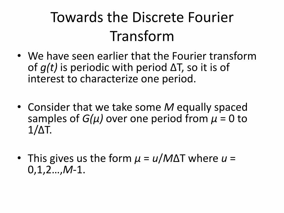
• We have seen earlier that the Fourier transform of g(t) is periodic with period ΔT, so it is of interest to characterize one period.

• Consider that we take some M equally spaced samples of G(μ) over one period from μ = 0 to 1/ΔT.

• This gives us the form μ = u/MΔT where u = 0,1,2…,M-1.

Towards the Discrete Fourier Transform

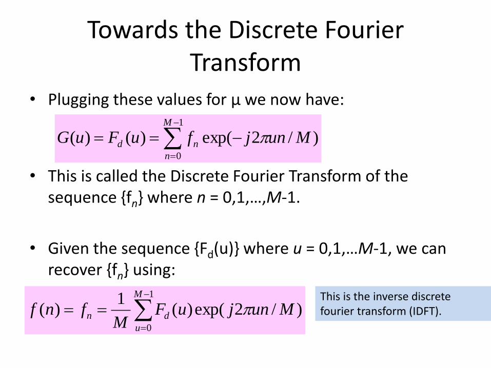
• Plugging these values for μ we now have:

• This is called the Discrete Fourier Transform of the sequence {fn} where n = 0,1,…,M-1.

• Given the sequence {Fd(u)} where u = 0,1,…M-1, we can recover {fn} using:

)/2exp()()(1

0

MunjfuFuGM

n

nd

)/2exp()(1

)(1

0

MunjuFM

fnfM

u

dn

This is the inverse discrete fourier transform (IDFT).

Towards the Discrete Fourier Transform

• Consider:

• It can be proved that plugging in the expression for f(n) into the expression for Fd (u) yields the identity Fd (u) = Fd (u).

• Also plugging in the expression for Fd (u) into the expression for f(n) yields the identity f(n) = f(n).

)/2exp()()(1

0

MunjfuFuGM

n

nd

)/2exp()(1

)(1

0

MunjuFM

nfM

u

d

Towards the Discrete Fourier Transform

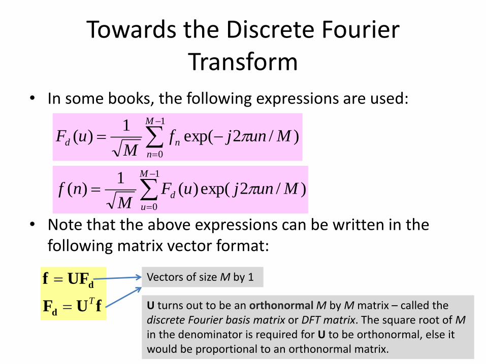
• In some books, the following expressions are used:

• Note that the above expressions can be written in the following matrix vector format:

)/2exp(1

)(1

0

MunjfM

uFM

n

nd

)/2exp()(1

)(1

0

MunjuFM

nfM

u

d

fUF

UFf

d

d

T

Vectors of size M by 1

U turns out to be an orthonormal M by M matrix – called the discrete Fourier basis matrix or DFT matrix. The square root of M in the denominator is required for U to be orthonormal, else it would be proportional to an orthonormal matrix.

)1(

.

.

)1(

)0(

..

.....

.....

..

..

1

)1(

.

.

)1(

)0(

domain realdomain,complex ;,,,

/)1)(1(2/)1)(1(2/)0)(1(2

/)1)(1(2/)1)(1(2/)0)(1(2

/)1)(0(2/)1)(0(2/)0)(0(2

MF

F

F

eee

eee

eee

M

Mf

f

f

d

d

d

MMMjMMjMMj

MMjMjMj

MMjMjMj

MMM

d

M

d

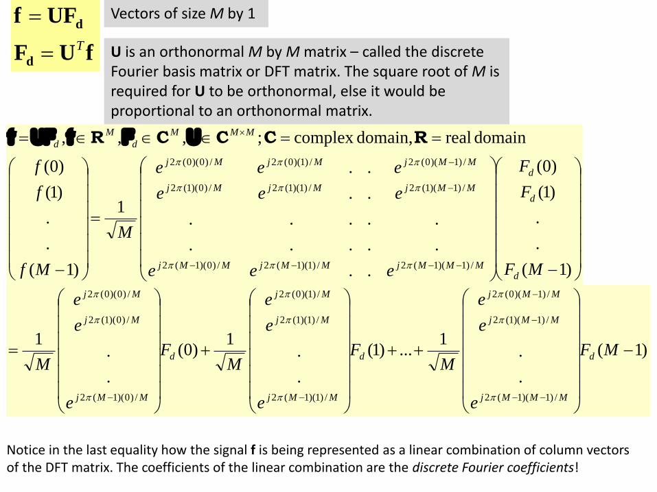
RCCCR UFfUFf

fUF

UFf

d

d

T

Vectors of size M by 1

U is an orthonormal M by M matrix – called the discrete Fourier basis matrix or DFT matrix. The square root of M is required for U to be orthonormal, else it would be proportional to an orthonormal matrix.

Notice in the last equality how the signal f is being represented as a linear combination of column vectors of the DFT matrix. The coefficients of the linear combination are the discrete Fourier coefficients!

)1(

.

.1

...)1(

.

.1

)0(

.

.1

/)1)(1(2

/)1)(1(2

/)1)(0(2

/)1)(1(2

/)1)(1(2

/)1)(0(2

/)0)(1(2

/)0)(1(2

/)0)(0(2

MF

e

e

e

MF

e

e

e

MF

e

e

e

Md

MMMj

MMj

MMj

d

MMj

Mj

Mj

d

MMj

Mj

Mj

Sampling in time and frequency

• Remember that the function g(t) was created by sampling f(t) with a period of ΔT.

• And the spacing between the samples in the frequency domain (to get the DFT from G(μ)) is

1/ ΔT since μ = u/MΔT where u = 0,1,2…,M-1.

• Likewise the range of frequencies spanned by the DFT is also inversely proportional to ΔT.

DFT properties

• Linearity: F(af+bg)(u) = aF(f)(u) + bF(g)(u)

• Periodicity: F(u) = F(u + kM) for integer k,

• And so is the inverse DFT since f(n) = f(n+kM).

• The DFT is in general complex. Hence it has a magnitude |F(u)| and a phase.

Clarification about DFT• We have seen earlier that the Fourier transform G(μ) of the sampled version g(t) of analog

signal f(t) is continuous.

• We also saw earlier that we take some M equally spaced samples of G(μ) over one period from μ = 0 to 1/ΔT.

• This way the DFT and the discrete signal both were vectors of M elements.

• Obtaining the DFT given the signal (or the signal given its DFT) is an efficient operation owing to the orthonormality of the discrete fourier matrix (why efficient? Because for an orthonormal matrix, inverse = transpose).

• Why don’t we take more than M samples in the frequency domain?

• If we did, the aforementioned computational efficiency would be lost. The inverse transform would require a matrix pseudo-inverse which is costly.

• Also the columns of the orthonormal matrix UT(size M x M) constitute a basis: i.e. any vector in M-dimensional space can be uniquely represented using linear combination of the columns of that matrix. If you took more than M samples in the frequency domain, that uniqueness would be lost as UT would now have size M’ x M where M’ > M.

Convolution of discrete signals

• Discrete equivalent of the convolution is:

• Due to the periodic nature of the DFT and IDFT, the convolution will also be periodic.

• The above formula represents one period of that periodic resultant signal.

1

0

)()())(*(M

m

mnhmfnhf

Convolution of discrete signals

• The convolution theorem from continuous signals has an extension to the discrete case as well:

• Therefore discrete convolution can be implemented using product of DFTs followed by an IDFT.

• But in doing so, one has to account for periodicityissues to avoid wrap-around artifacts (see next slide).

)()())(*( uHuFuhf F

Convolution of discrete signals• Consider the discrete convolution:

• To convolve f with h, you need to (1) flip h about the origin, (2) translate the flipped signal by an amount n, and (3) compute the sum in the above formula.

• Steps 2 and 3 are repeated for each value of n.

• The variable n ranges over all integers required to completely slide h over f.

• If h and f have size M, then n has to range up to 2M-1.

1

0

)()())(*(M

l

lnhlfnhf

Convolution of discrete signals• In other words, the resultant signal must have length of

2M-1.

• The convolution can be implemented in the time/spatial domain – and MATLAB has a routine called conv which does the job for you!

• Now imagine you tried to implement the convolution using a DFT of M-point signals followed by an M-point IDFT.

• Owing to the assumed periodicity, you would get an undesirable wrap-around effect. See next slide for an illustration.

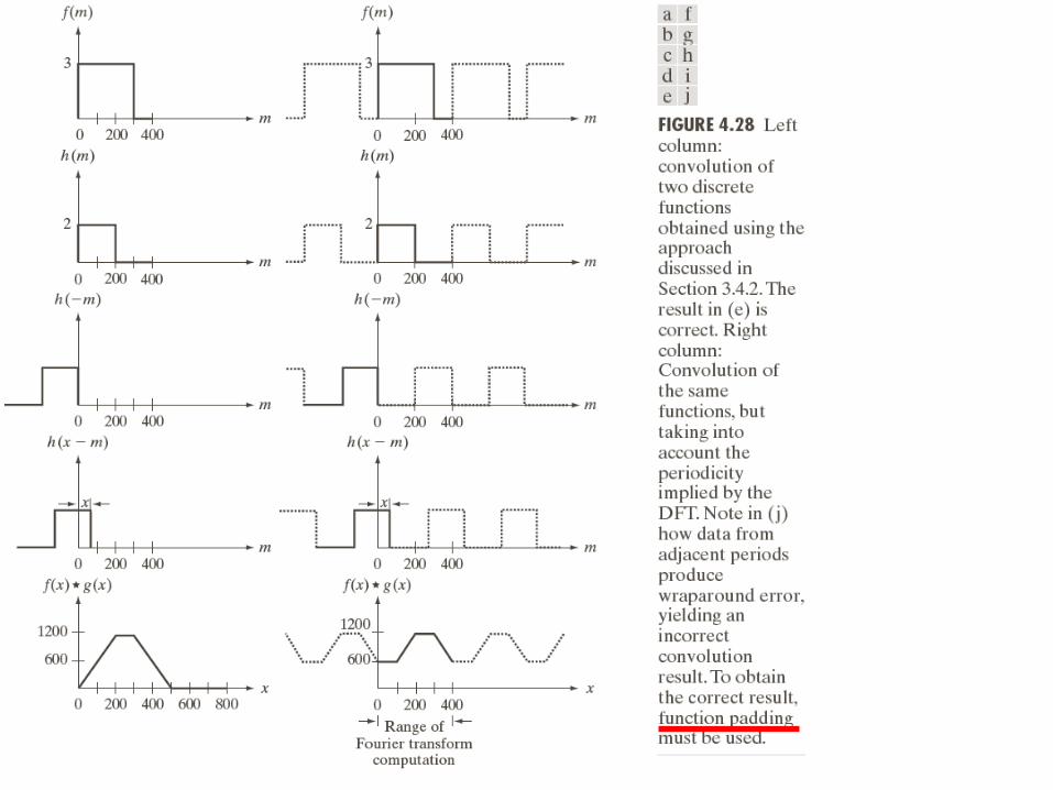
Convolution of discrete signals• How does one deal with this conundrum?

• If f has length M and h has length K, then you should zero-pad both sequences so that they now have length at least M+K-1.

• Then compute M+K-1 point DFT for both, multiply the DFTs and compute the M+K-1 point IDFT.

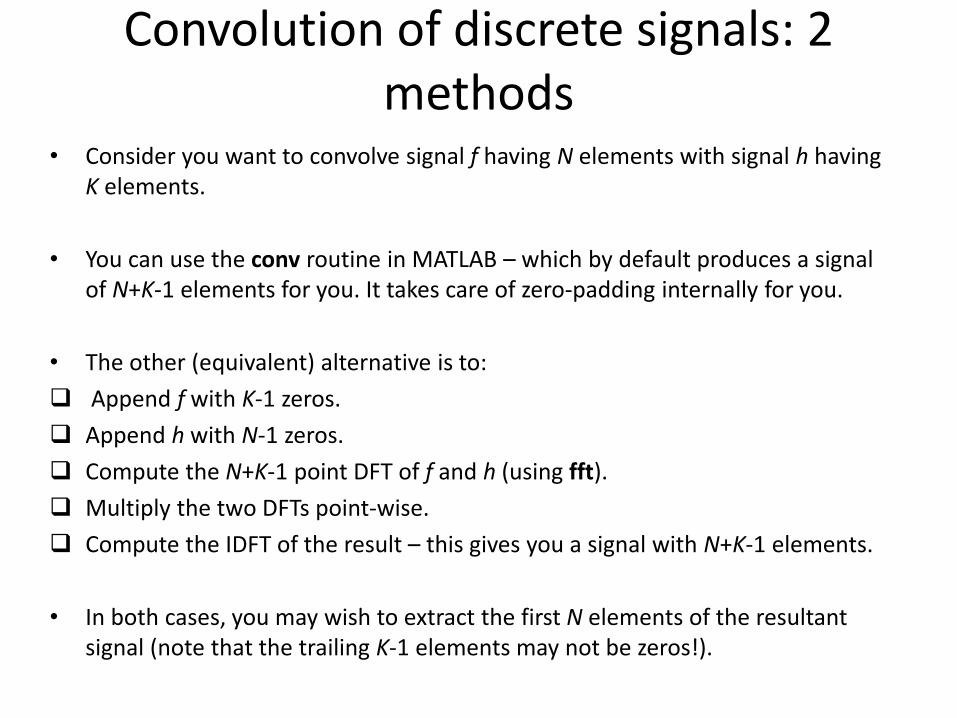
Convolution of discrete signals: 2 methods

• Consider you want to convolve signal f having N elements with signal h having K elements.

• You can use the conv routine in MATLAB – which by default produces a signal of N+K-1 elements for you. It takes care of zero-padding internally for you.

• The other (equivalent) alternative is to:

Append f with K-1 zeros.

Append h with N-1 zeros.

Compute the N+K-1 point DFT of f and h (using fft).

Multiply the two DFTs point-wise.

Compute the IDFT of the result – this gives you a signal with N+K-1 elements.

• In both cases, you may wish to extract the first N elements of the resultant signal (note that the trailing K-1 elements may not be zeros!).

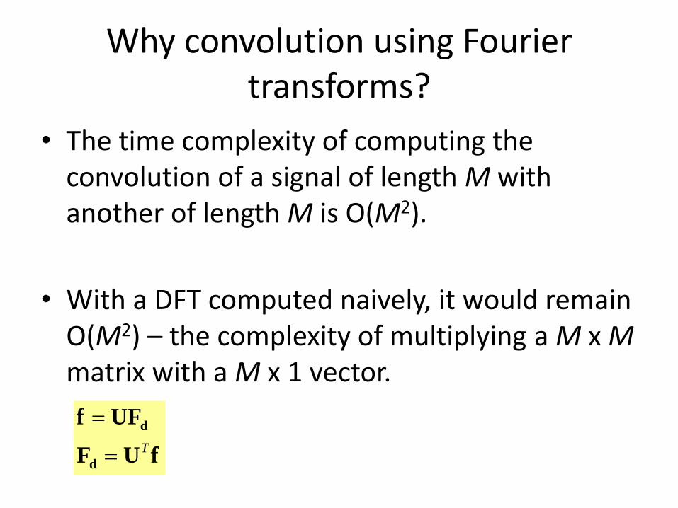
Why convolution using Fourier transforms?

• The time complexity of computing the convolution of a signal of length M with another of length M is O(M2).

• With a DFT computed naively, it would remain O(M2) – the complexity of multiplying a M x Mmatrix with a M x 1 vector.

fUF

UFf

d

d

T

Why convolution using Fourier transforms?

• But there’s a smarter way of doing the same which computes the DFT in O(M log M) time.

• That is called the Fast Fourier Transform, discovered by Cooley and Tukey in 1965.

• It is based on a divide and conquer algorithmic strategy.

• The same strategy can be used to compute the IDFT in O(Mlog M) time.

• Hence convolution can now be computed in O(M log M) time.

Towards the Fast Fourier Transform

)/2exp( where

)/2exp()(1

0

1

0

MjW

WfMunjfuF

M

un

M

M

n

n

M

n

n

KM n 22Let

)12(

2

1

0

12

)2(

2

1

0

22

12

0

)(

nu

K

K

n

n

nu

K

K

n

n

un

K

K

n

n WfWfWfuF

Even indicesOdd indices

u

K

nu

K

K

n

n

nu

K

K

n

n WWfWfuF 2

)(1

0

12

)(1

0

2)(

)()2(

2

nu

K

nu

K WW

Towards the Fast Fourier Transform

u

K

nu

K

K

n

n

nu

K

K

n

n WWfWfuF 2

)(1

0

12

)(1

0

2)(

u

K

u

K

K

K

u

K

Ku

K

u

Koddeven

u

Koddeven

nu

K

K

n

nodd

nu

K

K

n

neven

WKKjWWWW

KuWuFuFKuF

KuWuFuFuF

WfuFWfuF

22222

2

2

)(1

0

12

)(1

0

2

)2/2exp( as

1,...,1,0for )()()( and

1,...,1,0for )()()(

)(,)( Define

The M-point DFT computation for F is split up into two halves. The first half requirestwo M/2-point DFT computations – one for Feven, one for Fodd. The second half followsdirectly without any additional transform evaluations once Feven and Fodd are computed.Now Feven and Fodd can be further split up recursively.

Towards the Fast Fourier Transform

The M-point DFT computation for F is split up into two halves. The first halfrequires two M/2-point DFT computations – one for Feven, one for Fodd. Thesecond half follows directly without any additional transform evaluations onceFeven and Fodd are computed. Now Feven and Fodd can be further split uprecursively.This gives:

)log(

)2/(2

...

2)2/(2)2/)4/(2(2

)2/(2)(

(constant) )1(

22

MMO

kMMT

MMTMMMT

MMTMT

cT

kk

There is also a fast inverse Fourier transform which works quite similarly in O(M log M) time. The speedup achieved by the fast fourier transform over a naïve DFT computation is rather dramatic for large M!

M

T(M)

MATLAB implementation

• The Fast Fourier Transform is implemented in MATLAB directly – there are the routines fftand ifft for the inverse.

2D-DFT

• Given a 2D discrete signal (image) f(x,y) of size W1 by W2, its DFT is given as:

))//(2exp(),(1

),( 21

1

0

1

021

1 2

WvyWuxjyxfWW

vuFW

x

W

y

d

))//(2exp(),(1

),( 21

1

0

1

021

1 2

WvyWuxjvuFWW

yxfW

u

W

v

2D-DFT computation

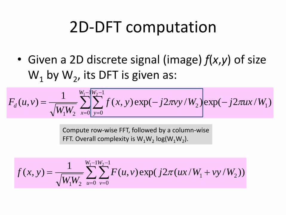
• Given a 2D discrete signal (image) f(x,y) of size W1 by W2, its DFT is given as:

)/2exp()/2exp(),(1

),( 12

1

0

1

021

1 2

WuxjWvyjyxfWW

vuFW

x

W

y

d

))//(2exp(),(1

),( 21

1

0

1

021

1 2

WvyWuxjvuFWW

yxfW

u

W

v

Compute row-wise FFT, followed by a column-wise FFT. Overall complexity is W1W2 log(W1W2).

MATLAB implementation

• The FFT for 2D arrays or images is implemented in MATLAB routines fft2 and ifft2.

2D-DFT properties

• Linearity: F(af+bg)(u,v) = aF(f)(u,v) + bF(g)(u,v) where a and b are scalars.

• Periodicity: F(u,v) = F(u + k1W1,v) = F(u,v + k2W2)=F(u + k1W1,v + k2W2) for integer k1 and k2.

• And so is the inverse DFT since f(x,y) = f(x + k1W1,y) = f(x,y + k2W2)= f(x + k1W1,y + k2W2) for integer k1 and k2.

2D-DFT: Magnitude and phase

• The phase carries very critical information.

• If you retain the magnitude of the Fourier transform of an image, but change its phase, the appearance drastically changes.

Magnitude of FT of Salman Khan, and phase of P V Sindhu

Magnitude of FT of P V Sindhu, and phase of Salman Khan

2D-DFT properties

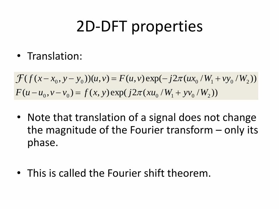
• Translation:

• Note that translation of a signal does not change the magnitude of the Fourier transform – only its phase.

• This is called the Fourier shift theorem.

))//(2exp(),(),(

))//(2exp(),(),))(,((

201000

201000

WyvWxujyxfvvuuF

WvyWuxjvuFvuyyxxf

F

Application in image alignment

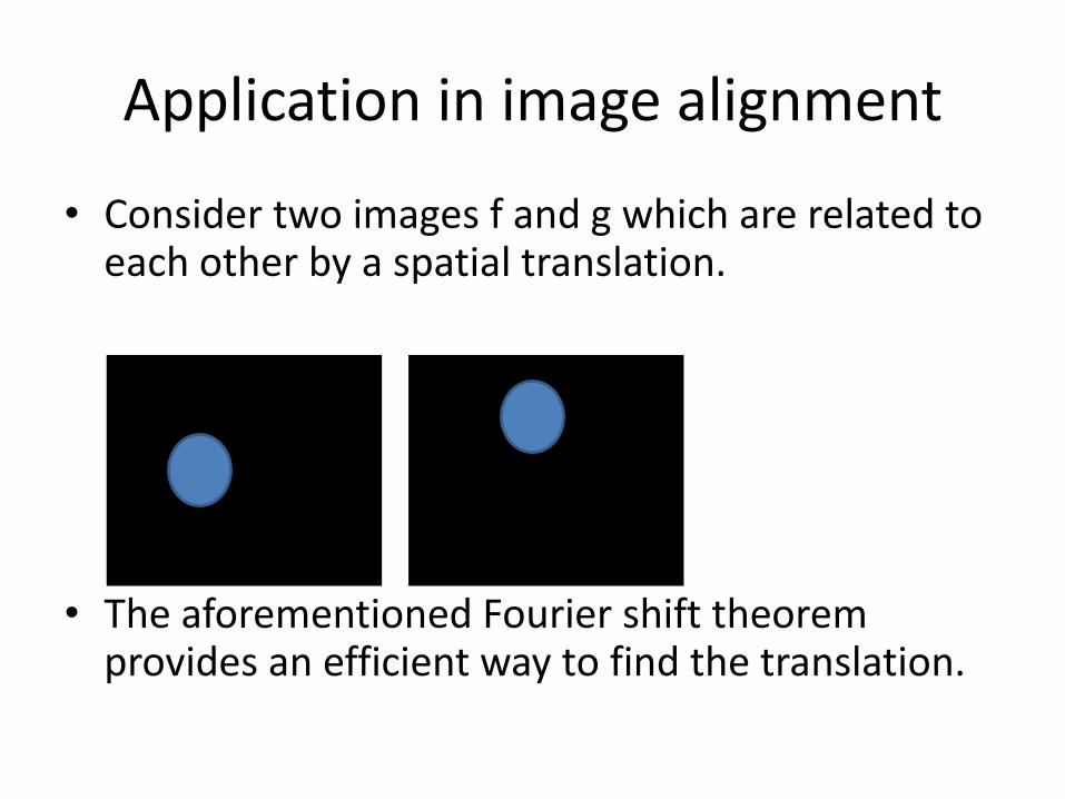
• Consider two images f and g which are related to each other by a spatial translation.

• The aforementioned Fourier shift theorem provides an efficient way to find the translation.

Application in image alignment

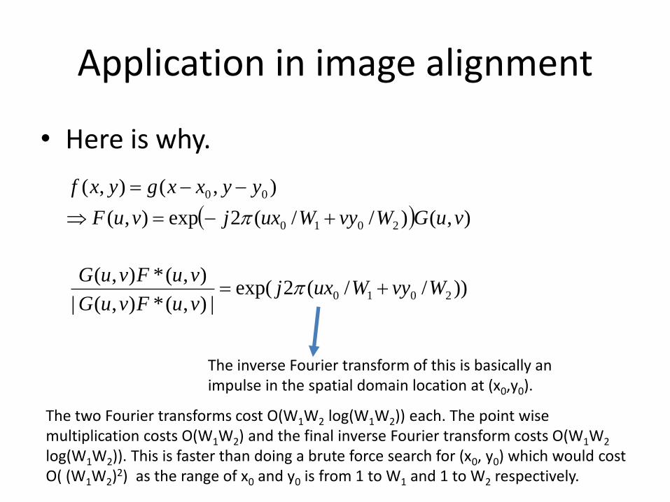
• Here is why.

),()//(2exp),(

),(),(

2010

00

vuGWvyWuxjvuF

yyxxgyxf

))//(2exp(|),(*),(|

),(*),(2010 WvyWuxj

vuFvuG

vuFvuG

The inverse Fourier transform of this is basically an impulse in the spatial domain location at (x0,y0).

The two Fourier transforms cost O(W1W2 log(W1W2)) each. The point wise multiplication costs O(W1W2) and the final inverse Fourier transform costs O(W1W2

log(W1W2)). This is faster than doing a brute force search for (x0, y0) which would cost O( (W1W2)2) as the range of x0 and y0 is from 1 to W1 and 1 to W2 respectively.

2D-DFT properties

• The Fourier transform of a rotated image yields a rotated version of its Fourier transform

• If you consider conversion to polar coordinates, then we have:

)cossin,sincos(

),))(cossin,sincos((

),(),))(,((

vuvuF

vuyxyxf

vuFvuyxf

F

F

sin,cos

sin,cos

vu

ryrx

))sin(),cos((

),)))(sin(),cos(((

),(),))(,((

F

vurrf

vuFvuyxf

F

F

2D-DFT visualization in MATLAB

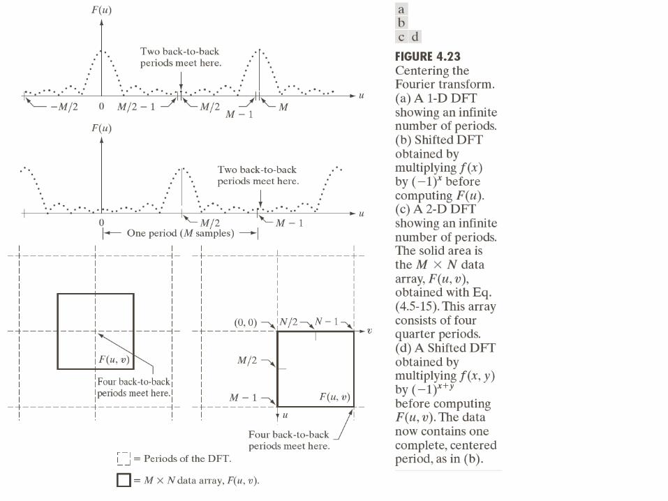
• In the formula for the DFT, the frequency range from u= 0 to u = M-1 actually represents two half periods back to back meeting at M/2 (see next slide).

• It is more convenient to instead view a complete period of the DFT instead.

• For that purpose we visualize F(u-M/2) instead of F(u) in 1D, and F(u-W1/2,v-W2/2) instead of F(u,v) in 2D.

• Thereby frequency u = 0 or u = v = 0 now occurs at the center of the displayed Fourier transform.

• Note that F(u-W1/2,v-W2/2) = F(f(x,y)(-1)x+y)(u,v), so the centering operation is easy to implement.

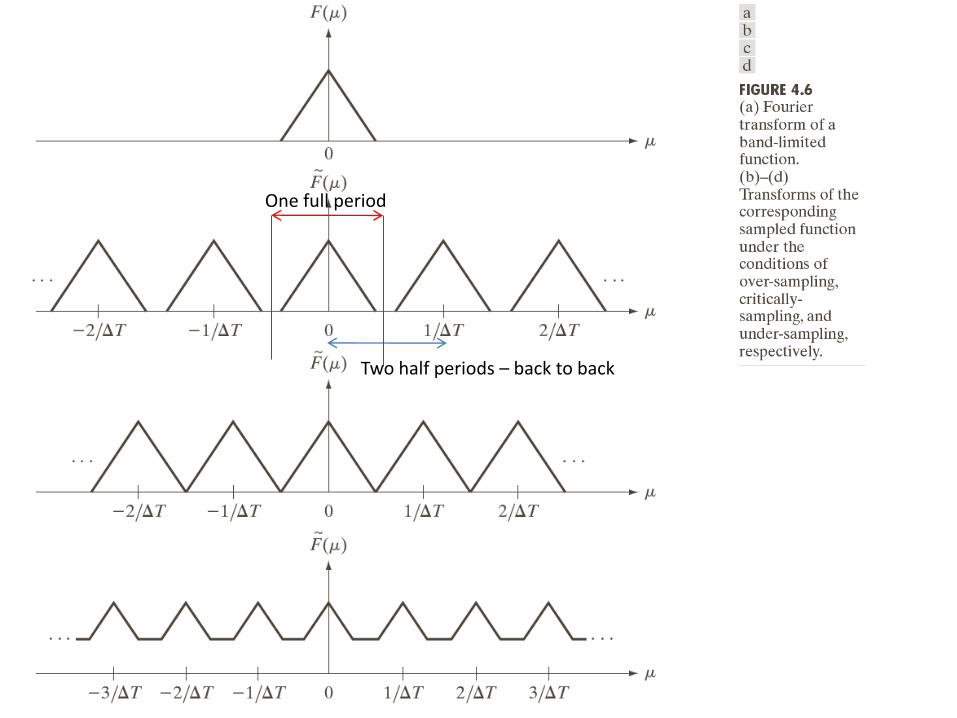
One full period

Two half periods – back to back

2D-DFT visualization in MATLAB

• To visualize the DFT of an image, we visualize the magnitude of the DFT.

• The Fourier transform is first centered as mentioned on the previous slide.

• Due to the large range of magnitude values, the DFT magnitudes are visualized on a logarithmic scale, i.e. we view log(|F(u,v)|+1) where the 1 is added for stability.

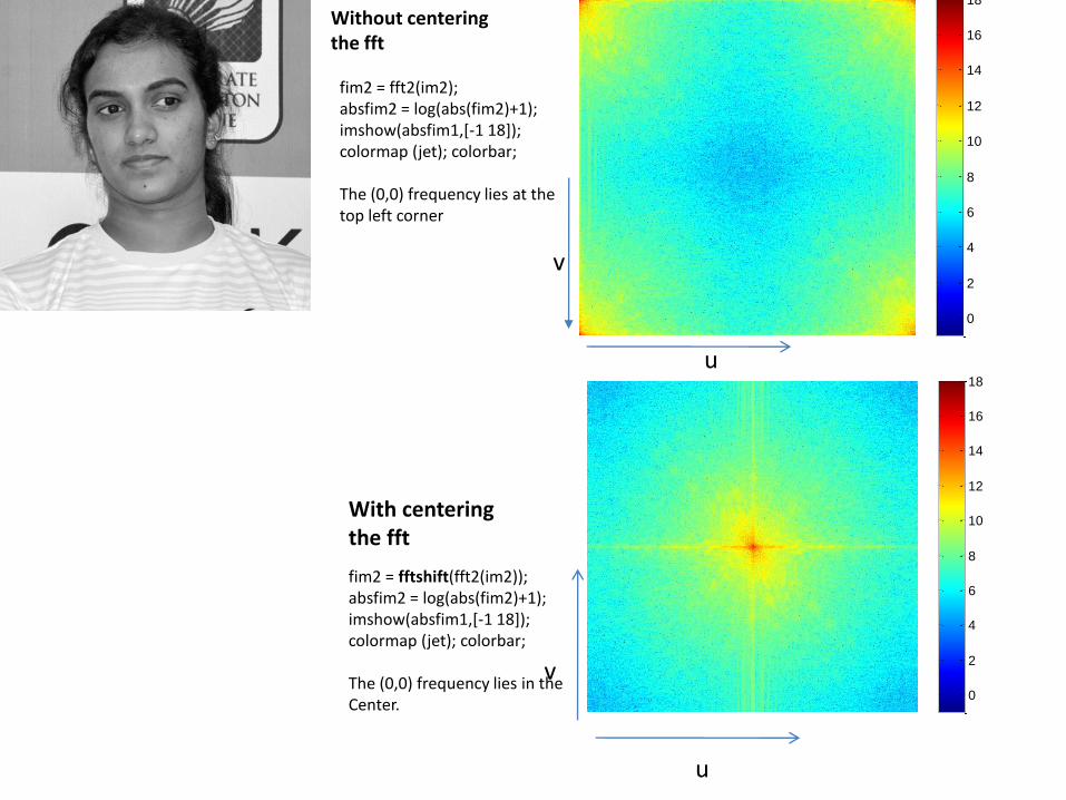
fim2 = fft2(im2); absfim2 = log(abs(fim2)+1); imshow(absfim1,[-1 18]); colormap (jet); colorbar;

The (0,0) frequency lies at the top left corner

Without centering the fft

0

2

4

6

8

10

12

14

16

18

0

2

4

6

8

10

12

14

16

18

fim2 = fftshift(fft2(im2)); absfim2 = log(abs(fim2)+1); imshow(absfim1,[-1 18]); colormap (jet); colorbar;

The (0,0) frequency lies in theCenter.

With centering the fft

u

v

u

v

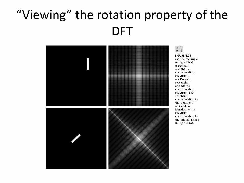
“Viewing” the rotation property of the DFT

2D convolution

• In MATLAB, 2D convolution can be implemented using the routine conv2.

• This can be very expensive if the signals you wish to convolve another with, are of large size.

• Hence one resorts to the convolution theorem which holds in 2D as well.

2D convolution• The convolution theorem applies to 2D-DFTs as

well:

• Consider an image f of size W1 x W2 which you want to convolve with a kernel k of size K1 x K2using the DFT method.

• Then you should symmetrically zero-pad f and kso that they acquire size W1+K1-1 x W2+K2-1.

• Compute the DFTs of the zero-padded images using the FFT algorithm, point-wise multiply them and obtain the IDFT of the result.

• Extract the central W1 x W2 portion of the result –for the final answer.

),(),(),)(*( vuHvuFvuhf F

Image Filtering: Frequency domain

• You have studied image filters of various types: mean filter, Gaussian filter, bilateral filter, patch-based filter.

• The former two are linear filters and the latter two aren’t.

• Linear filters are represented using convolutions and hence have a frequency domain interpretation as seen on the previous slides.

Image Filtering: Frequency domain

• Hence such filters can also be designed in the frequency domain.

• In certain applications, it is in fact more intuitive to design filters directly in the frequency domain.

• Why? Because you get to design directly which frequency components to weaken/eliminate and which ones to boost, and by how much.

Low pass filters

• Edges and fine textures in images contribute significantly to the high frequency content of an image.

• When you smooth/blur an image, these edges and textures are weakened (or removed).

• Such filters allow only the low frequencies to remain intact and are called as low pass filters.

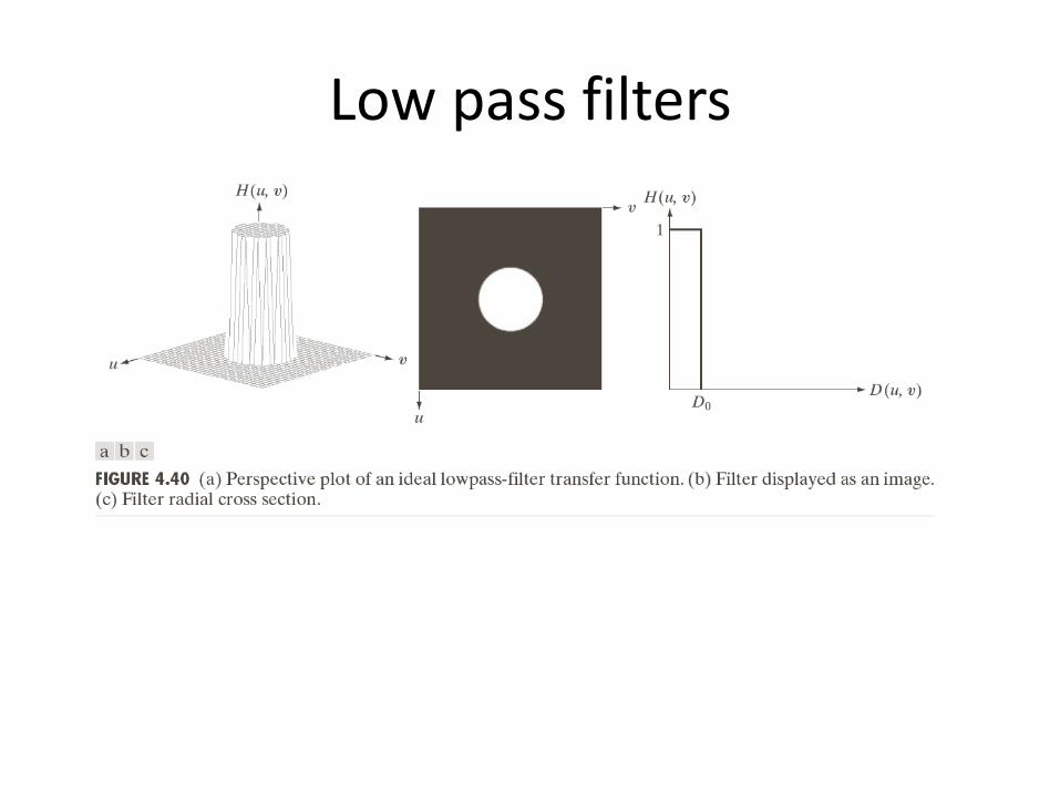
• In the frequency domain, an ideal low pass filter can be represented as follows:

otherwise 0

if ,1),( 222

DvuvuH Note: we are assuming (0,0) to be the center (lowest) frequency. Frequencies outside a radius of D from the center frequency are eliminated.

Low pass filters

Low pass filters

• To apply such a filter to an image f to create a filtered image g, we do as follows:

• D is a design parameter of the filter – often called the cutoff frequency.

• This is called the ideal low pass filter as it completely eliminates frequencies outside the chosen radius.

),(),(),(

otherwise 0

if ,1),( 222

vuHvuFvuG

DvuvuH

Low pass filters

Notice the ringing artifacts around the edges!

Low pass filters

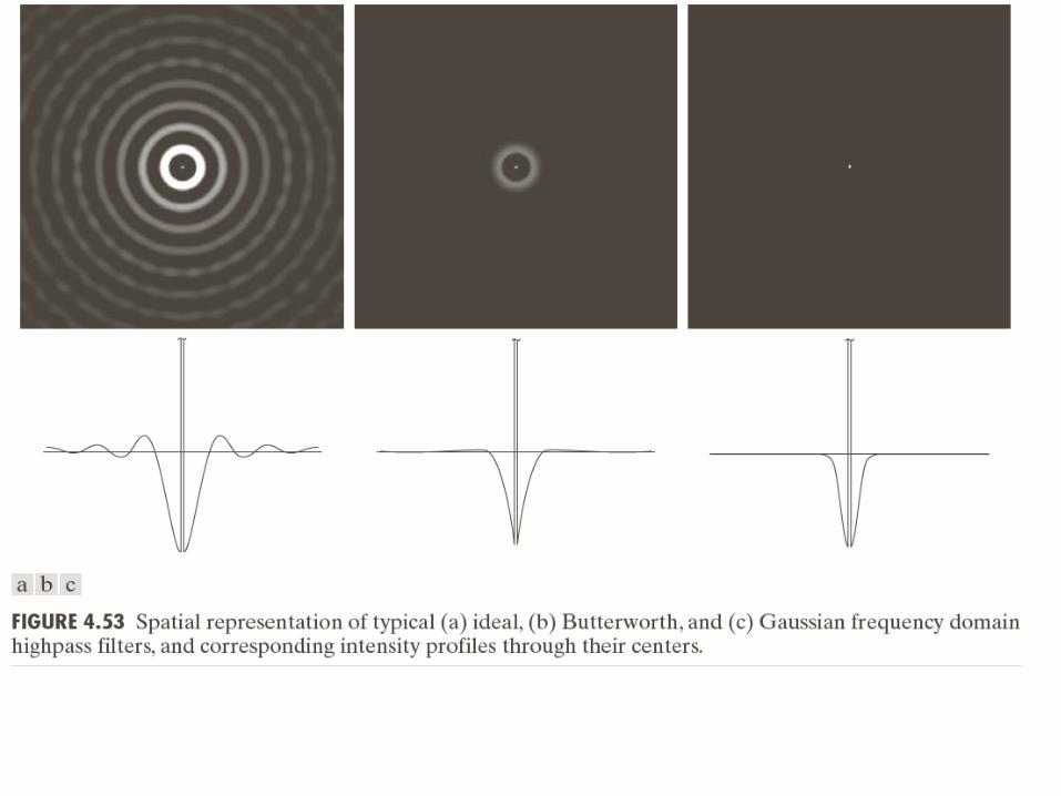
• The ringing artifacts can be explained by the convolution theorem.

• The corresponding spatial domain filter is called the jinc function.

• The jinc is a 2D and circularly symmetric version of the sincfunction – see also the next slide.

• Any cross section of the jinc is basically a sinc function.

https://en.wikipedia.org/wiki/Sombrero_function

An image can be regarded as a weighted sum of Kronecker delta functions (impulses). Convolving with a sinc function means placing copies of the sinc function at each impulse. The central lobe of the sinc function causes the blurring and the smaller lobes give rise to the “ripple artifacts” or ringing.

Low pass filters: other types

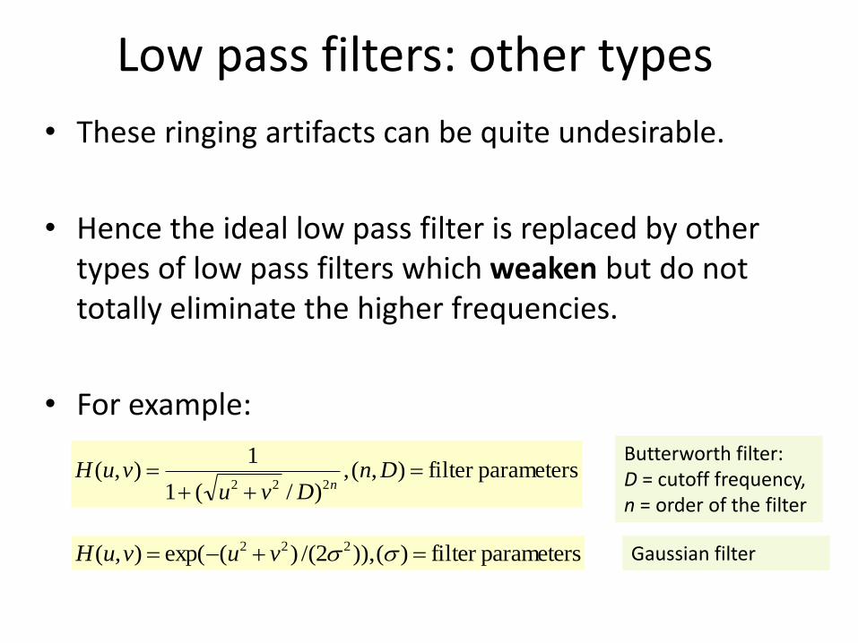
• These ringing artifacts can be quite undesirable.

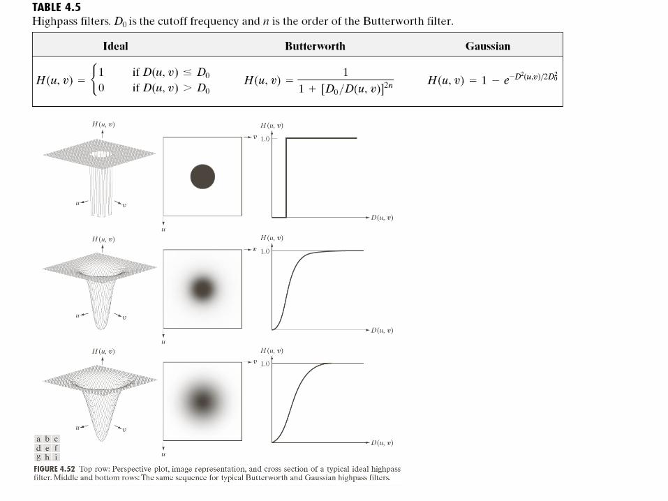
• Hence the ideal low pass filter is replaced by other types of low pass filters which weaken but do not totally eliminate the higher frequencies.

• For example:

parametersfilter ),(,)/(1

1),(

222

Dn

DvuvuH

n

parametersfilter )()),2/()(exp(),( 222 vuvuH

Butterworth filter:D = cutoff frequency, n = order of the filter

Gaussian filter

Low pass filters: Butterworth

• As D increases, the Butterworth filter allows more frequencies to pass through without weakening (see previous slide).

• As the order n increases, the Butterworth filter weakens the higher frequencies more aggressively (why?) – which actually increases ringing artifacts (see previous slide).

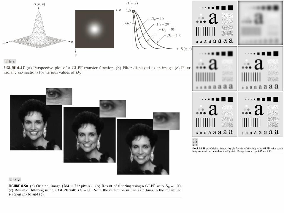
Low pass filters: Gaussian

• The spatial domain representation for the Gaussian LPF is basically a Gaussian.

• In fact, the following are Fourier transform pairs:

)/1(2exp)(

2exp

2

1)(

2

2

2

2

uuG

xxg

http://www.cse.yorku.ca/~kosta/CompVis_Notes/fourier_transform_Gaussian.pdf

Notice from the equations that a spatial domain Gaussian with high standard deviation corresponds to a frequency domain Gaussian with low cut off frequency! The extreme case of this is a constant intensity signal (Gaussian with very high standard deviation – infinite as such) whose Fourier transform is an impulse at the origin of the Frequency plane). Another extreme case is a spatial domain signal which is just an impulse – its Fourier transform has constant amplitude everywhere.

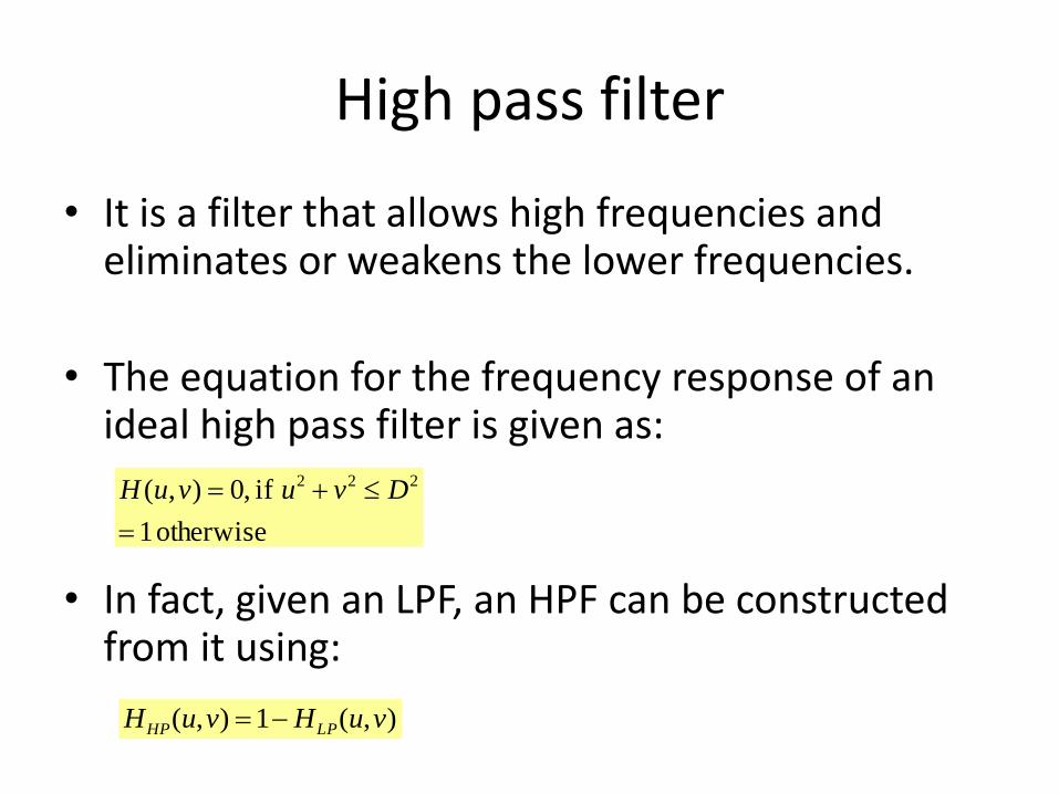
High pass filter

• It is a filter that allows high frequencies and eliminates or weakens the lower frequencies.

• The equation for the frequency response of an ideal high pass filter is given as:

• In fact, given an LPF, an HPF can be constructed from it using:

otherwise 1

if ,0),( 222

DvuvuH

),(1),( vuHvuH LPHP

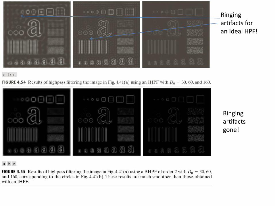
Ringing artifacts for an Ideal HPF!

Ringing artifacts gone!

Ringing artifacts for an Ideal HPF!

Ringing artifacts gone!

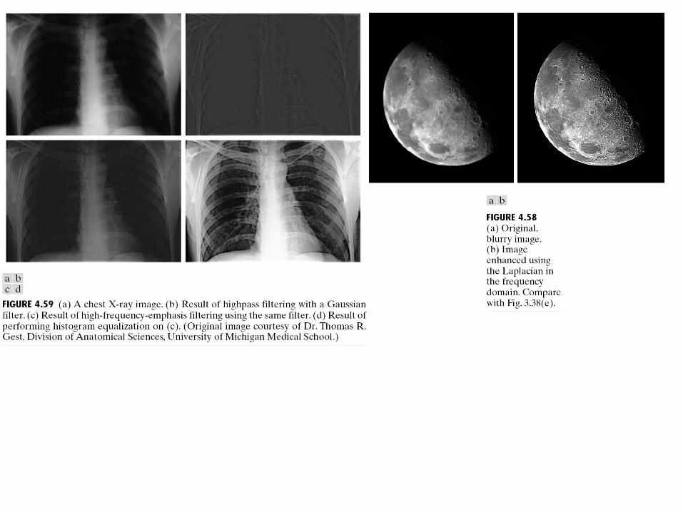
High pass filters

• Note that any gradient-based operation on images is essentially a type of high-pass filter.

• This includes first order derivative filters or the Laplacian filter.

• Why? Consider the first order derivative filter in y direction.

)1)(,(),(

),()1,(),(

/2 MvjevuIvuG

yxIyxIyxg

0)0,( uG

High pass filters

• Consider the Laplacian filter:

),(4

)4(),(

4/)),(4),1()1,(),1()1,((),(

/2/2/2/2

vuIeeee

vuG

yxIyxIyxIyxIyxIyxg

MujMvjMujMvj

0)0,0( G

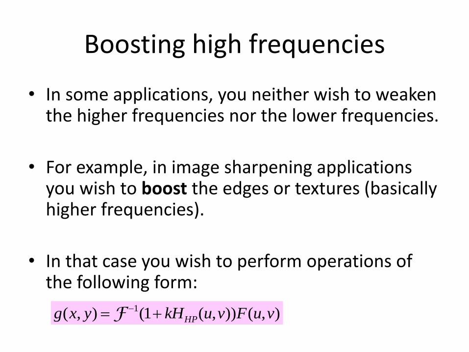
Boosting high frequencies

• In some applications, you neither wish to weaken the higher frequencies nor the lower frequencies.

• For example, in image sharpening applications you wish to boost the edges or textures (basically higher frequencies).

• In that case you wish to perform operations of the following form:

),()),(1(),( 1 vuFvukHyxg HP F

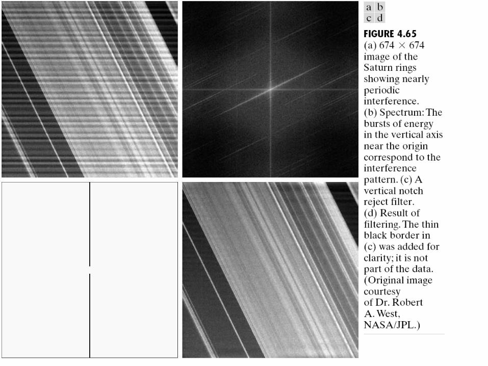
Notch filters

• There are applications where images are presented with periodic noise patterns – e.g. images scanned from old newspapers (see next slide).

• Usually, the amplitudes of the Fourier components of natural images are seen to decay with frequency.

• The Fourier transform of images with periodic patterns show unnatural peaks – unlike ordinary natural images.

• Such images can be restored using notch filters, which basically weaken or eliminate these unnatural frequency components (or any frequency components specified by the user).

The yellow ellipses indicate unnatural peaks in the Fourier transform of the image with the superimposed interfering pattern. These are unnatural because typical images do not have such Fourier transforms. Therefore one can apply a notch filter to remove the interfering pattern.

Courtesy: http://www.robots.ox.ac.uk/~az/lectures/ia/lect2.pdf

Courtesy: http://www.robots.ox.ac.uk/~az/lectures/ia/lect2.pdf

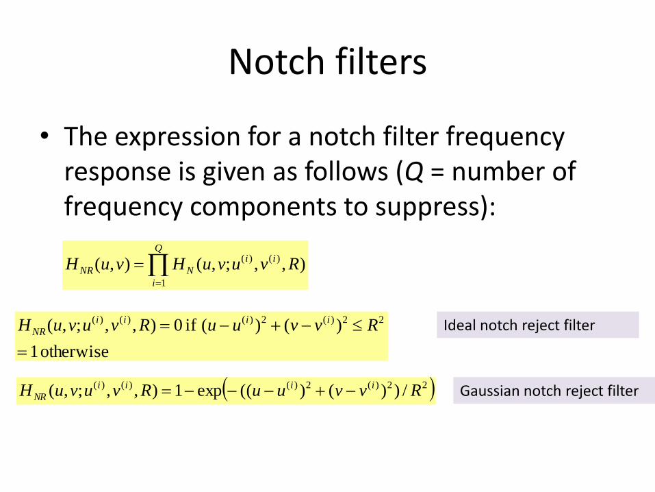
Notch filters

• The expression for a notch filter frequency response is given as follows (Q = number of frequency components to suppress):

),,;,(),( )()(

1

RvuvuHvuH iiQ

i

NNR

otherwise 1

)()( if 0),,;,( 22)(2)()()(

RvvuuRvuvuH iiii

NRIdeal notch reject filter

22)(2)()()( /))()((exp1),,;,( RvvuuRvuvuH iiii

NR Gaussian notch reject filter

Algorithm for frequency domain filtering

• Consider you have to filter an image f of size H x W using one of the filters described in these slides.

• Zero pad the image symmetrically to create a new image f’ of size 2H x 2W.

• Compute the Fourier transform of f’ and center it using fftshift. Let the Fourier transform be F’(u,v).

• Design a frequency domain filter H(u,v) of size 2H x 2W with the zero frequency at index (H,W) of the 2D filter array.

• Compute the product F’(u,v)H(u,v).• Compute the inverse Fourier transform of the product after applying

ifftshift (to undo the effect of fftshift).• Consider only the real part of the inverse Fourier transform and extract

the central portion of size H x W.• That gives you the final filtered image.• Note that the zero padding is important. To understand the difference, see

the results on the next slide with and without zero-padding.

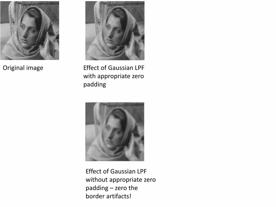
Effect of Gaussian LPF with appropriate zero padding

Original image

Effect of Gaussian LPF without appropriate zero padding – zero the border artifacts!

Interpreting the DFT of Natural Images

• In a few cases, one can guess some structural properties of an image by looking at its Fourier transform.

• Most natural images have stronger low frequency components as compared to higher frequency components. This is generally true, although its not a strictly monotonic relationship.

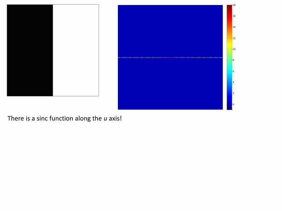
• For example, how does the DFT of a vertical edge image look like?

0

2

4

6

8

10

12

14

16

18

There is a sinc function along the u axis!

2

4

6

8

10

12

14

16

Strong horizontal and vertical edges = strong responses along u and v axes in the Fourier plane!

A strong edge in direction θ in XY plane = a strong response in the direction perpendicular to θin UV plane

Interpreting the DFT

• For an image (or any 2D array) with Fourier transform F(u,v), F(0,0) is proportional to the average value of the image intensity – why?

• The DFT of a non-zero constant intensity image is basically an impulse at the zero frequency. What is the height of the impulse?

DFT limitations

• A strong response at frequency (u,v) (i.e. a large magnitude for F(u,v)) indicates the presence of a sinusoid with frequency (u,v) and with large amplitude somewhere in the image.

• In general, the Fourier transform cannot and does not tell us where in the image the sinusoid is located (read section 1 of http://users.rowan.edu/~polikar/WAVELETS/WTpart1.html ).

• For that, you need to compute separate Fourier transforms over smaller regions of the image (Short time Fourier transform) – that will tell you which region(s) contained a particular sinusoidal component.

Fun with Fourier: Hybrid images

• Hybrid images are a superposition of an image J1 with strong low frequency components and weak higher frequency components, and an image J2 with stronger higher frequency components and weak lower frequency components.

• J1 = apply LPF with some cutoff frequency D on an image.• J2 = apply HPF with some cutoff frequency D on another

image.

• The appearance of the hybrid image changes with viewing distance!

Tiger – when seen up-close, Cheetah – when seen from far

Einstein from nearby, Marilyn Monroe from far away (or if you squint)!

Refer to:http://cvcl.mit.edu/hybrid_gallery/monroe_einstein.htmlhttp://cvcl.mit.edu/publications/OlivaTorralb_Hybrid_Siggraph06.pdf (paper from a graphics journal!)

Fourier in action: tomographic reconstruction

• Tomography refers to the process of estimation of the internal structure of an object (tomos in Greek means interior).

• This is different from photographic imaging which images only the object surface.

• Tomography is typically accomplished via X Rays and the so called Radon transform.

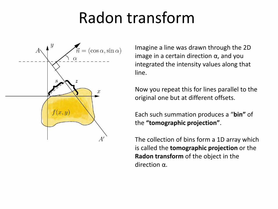
Radon transform

Imagine a line was drawn through the 2D image in a certain direction α, and you integrated the intensity values along that line.

Now you repeat this for lines parallel to the original one but at different offsets.

Each such summation produces a “bin” of the “tomographic projection”.

The collection of bins form a 1D array which is called the tomographic projection or the Radon transform of the object in the direction α.

Reconstruction from the Radon Transform

• The Radon transform computation can be similarly repeated for multiple angles.

• The aim of tomographic reconstruction is to reconstruct the 2D image from a collection of its 1D tomographic projections in different angles.

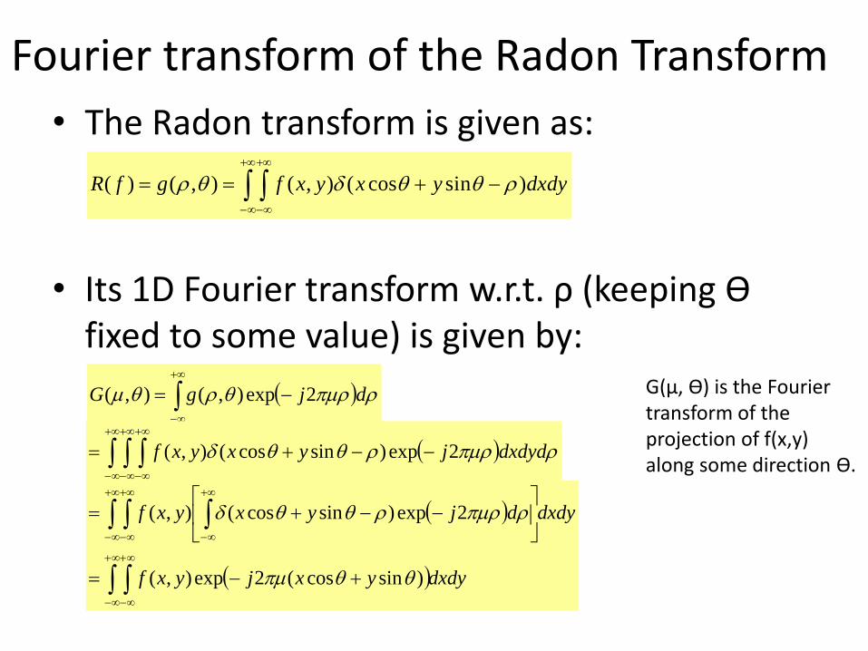
Fourier transform of the Radon Transform

• The Radon transform is given as:

• Its 1D Fourier transform w.r.t. ρ (keeping ϴfixed to some value) is given by:

dxdyyxyxfgfR )sincos(),(),()(

djgG 2exp),(),(

G(μ, ϴ) is the Fourier transform of the projection of f(x,y) along some direction ϴ.

dxdydjyxyxf 2exp)sincos(),(

dxdyyxjyxf

dxdydjyxyxf

)sincos(2exp),(

2exp)sincos(),(

Fourier transform of the Radon Transform

• Its 1D Fourier transform w.r.t. ρ (keeping ϴfixed) is given by:

sin,cos define wewhere

)(2exp),(

)sincos(2exp),(),(

vu

dxdyyvxujyxf

dxdyyxjyxfG

)sin,cos(),(),( sin,cos FvuFG vu

The RHS of this equation is a slice of the 2D Fourier transform of f(x,y), i.e. F(u,v), along the angle ϴ in the frequency plane, and passing through the origin

This equation above is called the Projection Slice Theorem or the Fourier Slice Theorem. It states that the Fourier transform of a projection of the 2D object along some direction ϴ(i.e. G(μ, ϴ)) is equal to a slice of the 2D Fourier transform of the object along the same direction ϴ (in the frequency plane), passing through the origin.

Reconstruction from the Radon transfer

• The projection slice theorem thus tells you that you can fill up the 2D Fourier transform of the original image – since the 1D Fourier transform of the projection at angle θ is equal to a slice of the 2D Fourier transform of the image at the angle θ through the origin of the (u,v) plane.

• Thus given different projections, each at different angles, you can fill up the Fourier transform of the original image. The final inverse Fourier transform gives you a reconstruction of the image.