Time Varying SDRs Ben Groom Individual Time Preferences The Social Discount Rate Time Varying Social Discount Rates Uncertainty Heterogeneity Risky Projects Estimating the Parameters of the SDR Conclusion Additional Materials Time Varying Social Discount Rates: Uncertainty, Heterogeneity and Project Risk Ben Groom (LSE) Centre for Health Economics, University of York December 7th, 2017

Welcome message from author
This document is posted to help you gain knowledge. Please leave a comment to let me know what you think about it! Share it to your friends and learn new things together.
Transcript
Time VaryingSDRs
Ben Groom
Individual TimePreferences
The SocialDiscount Rate
Time VaryingSocial DiscountRates
UncertaintyHeterogeneityRisky Projects
Estimating theParameters of theSDR
Conclusion
AdditionalMaterials
Time Varying Social Discount Rates:Uncertainty, Heterogeneity and Project Risk
Ben Groom (LSE)
Centre for Health Economics, University of YorkDecember 7th, 2017

Time VaryingSDRs
Ben Groom
Individual TimePreferences
The SocialDiscount Rate
Time VaryingSocial DiscountRates
UncertaintyHeterogeneityRisky Projects
Estimating theParameters of theSDR
Conclusion
AdditionalMaterials
Impatience, self-control and hyperbolic discounting
Figure: Source: The New Yorker.

Time VaryingSDRs
Ben Groom
Individual TimePreferences
The SocialDiscount Rate
Time VaryingSocial DiscountRates
UncertaintyHeterogeneityRisky Projects
Estimating theParameters of theSDR
Conclusion
AdditionalMaterials
Impatience, self-control and hyperbolic discounting
Figure: Source: The New Yorker.

Time VaryingSDRs
Ben Groom
Individual TimePreferences
The SocialDiscount Rate
Time VaryingSocial DiscountRates
UncertaintyHeterogeneityRisky Projects
Estimating theParameters of theSDR
Conclusion
AdditionalMaterials
The Social Discount RateRisk Free Projects
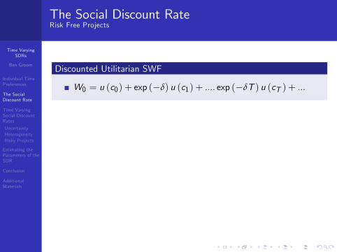
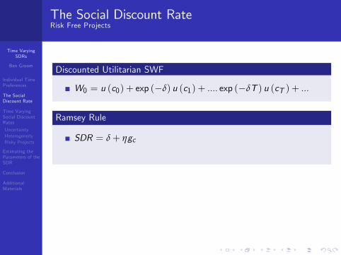
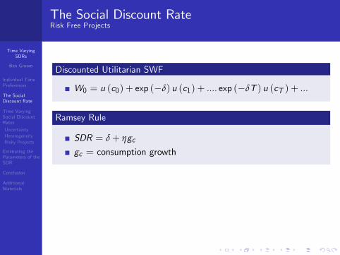
Discounted Utilitarian SWF
W0 = u (c0) + exp (�δ) u (c1) + .... exp (�δT ) u (cT ) + ...
Ramsey Rule
SDR = δ+ ηgcgc = consumption growth
2 consumption side arguments for discounting, 3 parameters (δ,η, gc )
1 Utility discounting: pure time preference, δ.
2 Societal �Wealth E¤ect�: ηgc
Time VaryingSDRs
Ben Groom
Individual TimePreferences
The SocialDiscount Rate
Time VaryingSocial DiscountRates
UncertaintyHeterogeneityRisky Projects
Estimating theParameters of theSDR
Conclusion
AdditionalMaterials
The Social Discount RateRisk Free Projects
Discounted Utilitarian SWF
W0 = u (c0) + exp (�δ) u (c1) + .... exp (�δT ) u (cT ) + ...
Ramsey Rule
SDR = δ+ ηgcgc = consumption growth
2 consumption side arguments for discounting, 3 parameters (δ,η, gc )
1 Utility discounting: pure time preference, δ.
2 Societal �Wealth E¤ect�: ηgc
Time VaryingSDRs
Ben Groom
Individual TimePreferences
The SocialDiscount Rate
Time VaryingSocial DiscountRates
UncertaintyHeterogeneityRisky Projects
Estimating theParameters of theSDR
Conclusion
AdditionalMaterials
The Social Discount RateRisk Free Projects
Discounted Utilitarian SWF
W0 = u (c0) + exp (�δ) u (c1) + .... exp (�δT ) u (cT ) + ...
Ramsey Rule
SDR = δ+ ηgc
gc = consumption growth
2 consumption side arguments for discounting, 3 parameters (δ,η, gc )
1 Utility discounting: pure time preference, δ.
2 Societal �Wealth E¤ect�: ηgc

Time VaryingSDRs
Ben Groom
Individual TimePreferences
The SocialDiscount Rate
Time VaryingSocial DiscountRates
UncertaintyHeterogeneityRisky Projects
Estimating theParameters of theSDR
Conclusion
AdditionalMaterials
The Social Discount RateRisk Free Projects
Discounted Utilitarian SWF
W0 = u (c0) + exp (�δ) u (c1) + .... exp (�δT ) u (cT ) + ...
Ramsey Rule
SDR = δ+ ηgcgc = consumption growth
2 consumption side arguments for discounting, 3 parameters (δ,η, gc )
1 Utility discounting: pure time preference, δ.
2 Societal �Wealth E¤ect�: ηgc
Time VaryingSDRs
Ben Groom
Individual TimePreferences
The SocialDiscount Rate
Time VaryingSocial DiscountRates
UncertaintyHeterogeneityRisky Projects
Estimating theParameters of theSDR
Conclusion
AdditionalMaterials
The Social Discount RateRisk Free Projects
Discounted Utilitarian SWF
W0 = u (c0) + exp (�δ) u (c1) + .... exp (�δT ) u (cT ) + ...
Ramsey Rule
SDR = δ+ ηgcgc = consumption growth
2 consumption side arguments for discounting, 3 parameters (δ,η, gc )
1 Utility discounting: pure time preference, δ.
2 Societal �Wealth E¤ect�: ηgc
Time VaryingSDRs
Ben Groom
Individual TimePreferences
The SocialDiscount Rate
Time VaryingSocial DiscountRates
UncertaintyHeterogeneityRisky Projects
Estimating theParameters of theSDR
Conclusion
AdditionalMaterials
The Social Discount RateRisk Free Projects
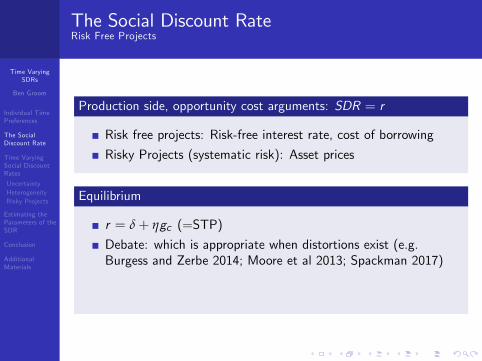
Production side, opportunity cost arguments: SDR = r
Risk free projects: Risk-free interest rate, cost of borrowing
Risky Projects (systematic risk): Asset prices
Equilibrium
r = δ+ ηgc (=STP)
Debate: which is appropriate when distortions exist (e.g.Burgess and Zerbe 2014; Moore et al 2013; Spackman 2017)
Shadow cost of capital approach: convert to consumption anddiscount using STP

Time VaryingSDRs
Ben Groom
Individual TimePreferences
The SocialDiscount Rate
Time VaryingSocial DiscountRates
UncertaintyHeterogeneityRisky Projects
Estimating theParameters of theSDR
Conclusion
AdditionalMaterials
The Social Discount RateRisk Free Projects
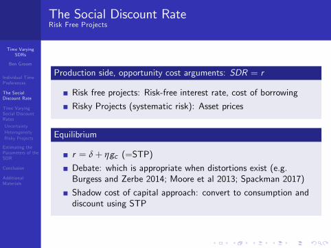
Production side, opportunity cost arguments: SDR = r
Risk free projects: Risk-free interest rate, cost of borrowing
Risky Projects (systematic risk): Asset prices
Equilibrium
r = δ+ ηgc (=STP)
Debate: which is appropriate when distortions exist (e.g.Burgess and Zerbe 2014; Moore et al 2013; Spackman 2017)
Shadow cost of capital approach: convert to consumption anddiscount using STP
Time VaryingSDRs
Ben Groom
Individual TimePreferences
The SocialDiscount Rate
Time VaryingSocial DiscountRates
UncertaintyHeterogeneityRisky Projects
Estimating theParameters of theSDR
Conclusion
AdditionalMaterials
The Social Discount RateRisk Free Projects
Production side, opportunity cost arguments: SDR = r
Risk free projects: Risk-free interest rate, cost of borrowing
Risky Projects (systematic risk): Asset prices
Equilibrium
r = δ+ ηgc (=STP)
Debate: which is appropriate when distortions exist (e.g.Burgess and Zerbe 2014; Moore et al 2013; Spackman 2017)
Shadow cost of capital approach: convert to consumption anddiscount using STP
Time VaryingSDRs
Ben Groom
Individual TimePreferences
The SocialDiscount Rate
Time VaryingSocial DiscountRates
UncertaintyHeterogeneityRisky Projects
Estimating theParameters of theSDR
Conclusion
AdditionalMaterials
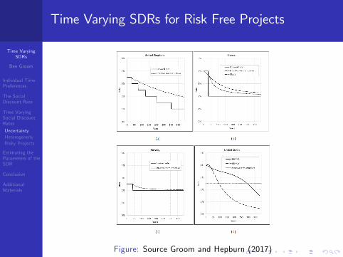
Time Varying SDRs for Risk Free Projects
Figure: Source Groom and Hepburn (2017)
Time VaryingSDRs
Ben Groom
Individual TimePreferences
The SocialDiscount Rate
Time VaryingSocial DiscountRates
UncertaintyHeterogeneityRisky Projects
Estimating theParameters of theSDR
Conclusion
AdditionalMaterials
Time Varying SDRs: Uncertainty in growthRisk Free Projects
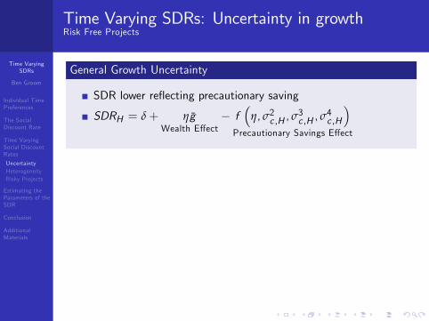
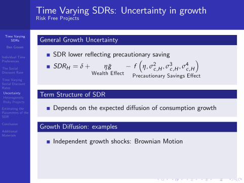
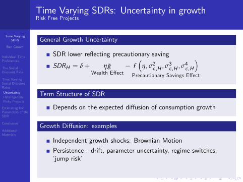
General Growth Uncertainty
SDR lower re�ecting precautionary saving
SDRH = δ+ ηgWealth E¤ect
� f�
η, σ2c ,H , σ3c ,H , σ
4c ,H
�Precautionary Savings E¤ect
Term Structure of SDR
Depends on the expected di¤usion of consumption growth
Growth Di¤usion: examples
Independent growth shocks: Brownian Motion
Persistence : drift, parameter uncertainty, regime switches,�jump risk�
See Gollier (2012)
Time VaryingSDRs
Ben Groom
Individual TimePreferences
The SocialDiscount Rate
Time VaryingSocial DiscountRates
UncertaintyHeterogeneityRisky Projects
Estimating theParameters of theSDR
Conclusion
AdditionalMaterials
Time Varying SDRs: Uncertainty in growthRisk Free Projects
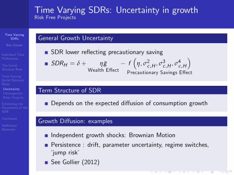
General Growth Uncertainty
SDR lower re�ecting precautionary saving
SDRH = δ+ ηgWealth E¤ect
� f�
η, σ2c ,H , σ3c ,H , σ
4c ,H
�Precautionary Savings E¤ect
Term Structure of SDR
Depends on the expected di¤usion of consumption growth
Growth Di¤usion: examples
Independent growth shocks: Brownian Motion
Persistence : drift, parameter uncertainty, regime switches,�jump risk�
See Gollier (2012)
Time VaryingSDRs
Ben Groom
Individual TimePreferences
The SocialDiscount Rate
Time VaryingSocial DiscountRates
UncertaintyHeterogeneityRisky Projects
Estimating theParameters of theSDR
Conclusion
AdditionalMaterials
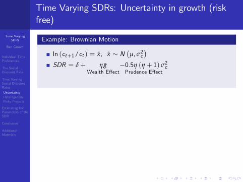
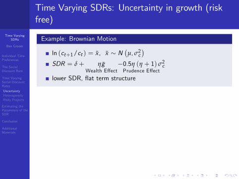
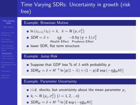
Time Varying SDRs: Uncertainty in growth (riskfree)
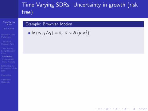
Example: Brownian Motion
ln (ct+1/ct ) = x , x � N�µ, σ2c
�SDR = δ+ ηg
Wealth E¤ect�0.5η (η + 1) σ2cPrudence E¤ect
lower SDR, �at term structure
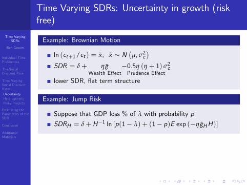
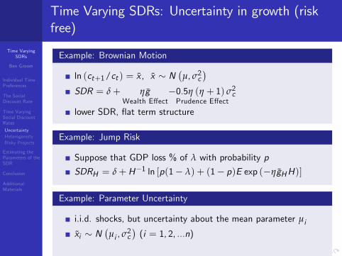
Example: Jump Risk
Suppose that GDP loss % of λ with probability p
SDRH = δ+H�1 ln [p(1� λ) + (1� p)E exp (�ηgHH)]
Example: Parameter Uncertainty
i.i.d. shocks, but uncertainty about the mean parameter µi
xi � N�µi , σ
2c�(i = 1, 2, ...n)
SDRH = δ+H�1 ln [E exp (�ηgHH)]
Time VaryingSDRs
Ben Groom
Individual TimePreferences
The SocialDiscount Rate
Time VaryingSocial DiscountRates
UncertaintyHeterogeneityRisky Projects
Estimating theParameters of theSDR
Conclusion
AdditionalMaterials
Time Varying SDRs: Uncertainty in growth (riskfree)
Example: Brownian Motion
ln (ct+1/ct ) = x , x � N�µ, σ2c
�
SDR = δ+ ηgWealth E¤ect
�0.5η (η + 1) σ2cPrudence E¤ect
lower SDR, �at term structure
Example: Jump Risk
Suppose that GDP loss % of λ with probability p
SDRH = δ+H�1 ln [p(1� λ) + (1� p)E exp (�ηgHH)]
Example: Parameter Uncertainty
i.i.d. shocks, but uncertainty about the mean parameter µi
xi � N�µi , σ
2c�(i = 1, 2, ...n)
SDRH = δ+H�1 ln [E exp (�ηgHH)]
Time VaryingSDRs
Ben Groom
Individual TimePreferences
The SocialDiscount Rate
Time VaryingSocial DiscountRates
UncertaintyHeterogeneityRisky Projects
Estimating theParameters of theSDR
Conclusion
AdditionalMaterials
Time Varying SDRs: Uncertainty in growth (riskfree)
Example: Brownian Motion
ln (ct+1/ct ) = x , x � N�µ, σ2c
�SDR = δ+ ηg
Wealth E¤ect�0.5η (η + 1) σ2cPrudence E¤ect
lower SDR, �at term structure
Example: Jump Risk
Suppose that GDP loss % of λ with probability p
SDRH = δ+H�1 ln [p(1� λ) + (1� p)E exp (�ηgHH)]
Example: Parameter Uncertainty
i.i.d. shocks, but uncertainty about the mean parameter µi
xi � N�µi , σ
2c�(i = 1, 2, ...n)
SDRH = δ+H�1 ln [E exp (�ηgHH)]
Time VaryingSDRs
Ben Groom
Individual TimePreferences
The SocialDiscount Rate
Time VaryingSocial DiscountRates
UncertaintyHeterogeneityRisky Projects
Estimating theParameters of theSDR
Conclusion
AdditionalMaterials
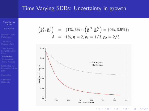
Time Varying SDRs: Uncertainty in growth
�gL1 , g
L2
�= (1%, 3%) ;
�gH1 , g
H2
�= (0%, 3.5%) ;
δ = 1%, η = 2, p1 = 1/3, p2 = 2/3
Time VaryingSDRs
Ben Groom
Individual TimePreferences
The SocialDiscount Rate
Time VaryingSocial DiscountRates
UncertaintyHeterogeneityRisky Projects
Estimating theParameters of theSDR
Conclusion
AdditionalMaterials
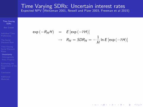
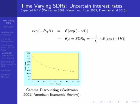
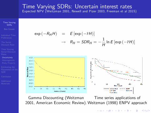
Time Varying SDRs: Uncertain interest ratesExpected NPV (Weitzman 2001, Newell and Pizer 2003, Freeman et al 2015)
exp (�RHH) = E [exp (�rH)]
! RH = SDRH = �1HlnE [exp (�rH)]
Gamma Discounting (Weitzman2001, American Economic Review).
Time series applications ofWeitzman (1998) ENPV approach
Time VaryingSDRs
Ben Groom
Individual TimePreferences
The SocialDiscount Rate
Time VaryingSocial DiscountRates
UncertaintyHeterogeneityRisky Projects
Estimating theParameters of theSDR
Conclusion
AdditionalMaterials
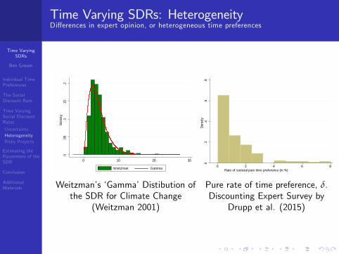
Time Varying SDRs: HeterogeneityDi¤erences in expert opinion, or heterogeneous time preferences
0.0
5.1
.15
.2De
nsity
0 10 20 30
Weitzman Gamma
Weitzman�s �Gamma�Distibution ofthe SDR for Climate Change
(Weitzman 2001)0
.2.4
.6.8
Dens
ity
0 2 4 6 8Rate of societal pure time preference (in %)
Pure rate of time preference, δ.Discounting Expert Survey by
Drupp et al. (2015)
Time VaryingSDRs
Ben Groom
Individual TimePreferences
The SocialDiscount Rate
Time VaryingSocial DiscountRates
UncertaintyHeterogeneityRisky Projects
Estimating theParameters of theSDR
Conclusion
AdditionalMaterials
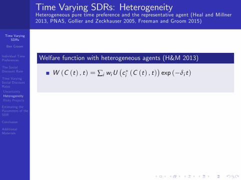
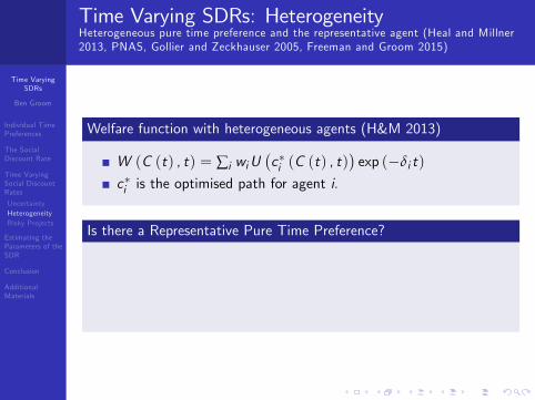
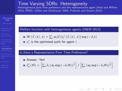
Time Varying SDRs: HeterogeneityHeterogeneous pure time preference and the representative agent (Heal and Millner2013, PNAS, Gollier and Zeckhauser 2005, Freeman and Groom 2015)
Welfare function with heterogeneous agents (H&M 2013)
W (C (t) , t) = ∑i wiU�c�i (C (t) , t)
�exp (�δi t)
c�i is the optimised path for agent i.
Is there a Representative Pure Time Preference?
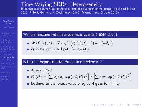
Answer: Yes!
δ�η (H) =h∑i δi (wi exp (�δiH))
1η
i/h∑i (wi exp (�δiH))
1η
iDeclines to the lowest value of δi as H goes to in�nity
Time VaryingSDRs
Ben Groom
Individual TimePreferences
The SocialDiscount Rate
Time VaryingSocial DiscountRates
UncertaintyHeterogeneityRisky Projects
Estimating theParameters of theSDR
Conclusion
AdditionalMaterials
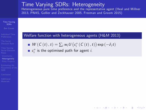
Time Varying SDRs: HeterogeneityHeterogeneous pure time preference and the representative agent (Heal and Millner2013, PNAS, Gollier and Zeckhauser 2005, Freeman and Groom 2015)
Welfare function with heterogeneous agents (H&M 2013)
W (C (t) , t) = ∑i wiU�c�i (C (t) , t)
�exp (�δi t)
c�i is the optimised path for agent i.
Is there a Representative Pure Time Preference?
Answer: Yes!
δ�η (H) =h∑i δi (wi exp (�δiH))
1η
i/h∑i (wi exp (�δiH))
1η
iDeclines to the lowest value of δi as H goes to in�nity

Time VaryingSDRs
Ben Groom
Individual TimePreferences
The SocialDiscount Rate
Time VaryingSocial DiscountRates
UncertaintyHeterogeneityRisky Projects
Estimating theParameters of theSDR
Conclusion
AdditionalMaterials
Time Varying SDRs: HeterogeneityHeterogeneous pure time preference and the representative agent (Heal and Millner2013, PNAS, Gollier and Zeckhauser 2005, Freeman and Groom 2015)
Welfare function with heterogeneous agents (H&M 2013)
W (C (t) , t) = ∑i wiU�c�i (C (t) , t)
�exp (�δi t)
c�i is the optimised path for agent i.
Is there a Representative Pure Time Preference?
Answer: Yes!
δ�η (H) =h∑i δi (wi exp (�δiH))
1η
i/h∑i (wi exp (�δiH))
1η
iDeclines to the lowest value of δi as H goes to in�nity
Time VaryingSDRs
Ben Groom
Individual TimePreferences
The SocialDiscount Rate
Time VaryingSocial DiscountRates
UncertaintyHeterogeneityRisky Projects
Estimating theParameters of theSDR
Conclusion
AdditionalMaterials
Time Varying SDRs: HeterogeneityHeterogeneous pure time preference and the representative agent (Heal and Millner2013, PNAS, Gollier and Zeckhauser 2005, Freeman and Groom 2015)
Welfare function with heterogeneous agents (H&M 2013)
W (C (t) , t) = ∑i wiU�c�i (C (t) , t)
�exp (�δi t)
c�i is the optimised path for agent i.
Is there a Representative Pure Time Preference?
Answer: Yes!
δ�η (H) =h∑i δi (wi exp (�δiH))
1η
i/h∑i (wi exp (�δiH))
1η
i
Declines to the lowest value of δi as H goes to in�nity
Time VaryingSDRs
Ben Groom
Individual TimePreferences
The SocialDiscount Rate
Time VaryingSocial DiscountRates
UncertaintyHeterogeneityRisky Projects
Estimating theParameters of theSDR
Conclusion
AdditionalMaterials
Time Varying SDRs: HeterogeneityHeterogeneous pure time preference and the representative agent (Heal and Millner2013, PNAS, Gollier and Zeckhauser 2005, Freeman and Groom 2015)
Welfare function with heterogeneous agents (H&M 2013)
W (C (t) , t) = ∑i wiU�c�i (C (t) , t)
�exp (�δi t)
c�i is the optimised path for agent i.
Is there a Representative Pure Time Preference?
Answer: Yes!
δ�η (H) =h∑i δi (wi exp (�δiH))
1η
i/h∑i (wi exp (�δiH))
1η
iDeclines to the lowest value of δi as H goes to in�nity
Time VaryingSDRs
Ben Groom
Individual TimePreferences
The SocialDiscount Rate
Time VaryingSocial DiscountRates
UncertaintyHeterogeneityRisky Projects
Estimating theParameters of theSDR
Conclusion
AdditionalMaterials
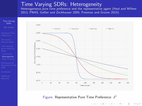
Time Varying SDRs: HeterogeneityHeterogeneous pure time preference and the representative agent (Heal and Millner2013, PNAS, Gollier and Zeckhauser 2005, Freeman and Groom 2015)
Figure: Representative Pure Time Preference: δ�
Time VaryingSDRs
Ben Groom
Individual TimePreferences
The SocialDiscount Rate
Time VaryingSocial DiscountRates
UncertaintyHeterogeneityRisky Projects
Estimating theParameters of theSDR
Conclusion
AdditionalMaterials
Time Varying SDRs with Risky ProjectsGollier (2012, 2012b)
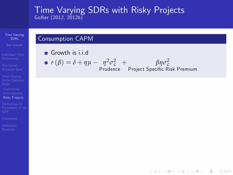
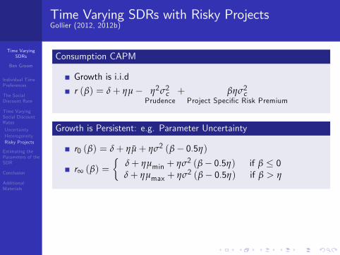
Consumption CAPM
Growth is i.i.d
r (β) = δ+ ηµ� η2σ2cPrudence
+ βησ2cProject Speci�c Risk Premium
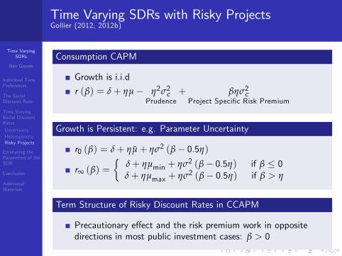
Growth is Persistent: e.g. Parameter Uncertainty
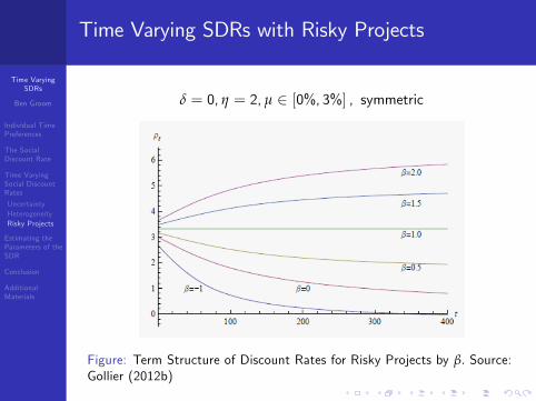
r0 (β) = δ+ ηµ+ ησ2 (β� 0.5η)
r∞ (β) =�
δ+ ηµmin + ησ2 (β� 0.5η) if β � 0δ+ ηµmax + ησ2 (β� 0.5η) if β > η
Term Structure of Risky Discount Rates in CCAPM
Precautionary e¤ect and the risk premium work in oppositedirections in most public investment cases: β > 0

Time VaryingSDRs
Ben Groom
Individual TimePreferences
The SocialDiscount Rate
Time VaryingSocial DiscountRates
UncertaintyHeterogeneityRisky Projects
Estimating theParameters of theSDR
Conclusion
AdditionalMaterials
Time Varying SDRs with Risky ProjectsGollier (2012, 2012b)
Consumption CAPM
Growth is i.i.d
r (β) = δ+ ηµ� η2σ2cPrudence
+ βησ2cProject Speci�c Risk Premium
Growth is Persistent: e.g. Parameter Uncertainty
r0 (β) = δ+ ηµ+ ησ2 (β� 0.5η)
r∞ (β) =�
δ+ ηµmin + ησ2 (β� 0.5η) if β � 0δ+ ηµmax + ησ2 (β� 0.5η) if β > η
Term Structure of Risky Discount Rates in CCAPM
Precautionary e¤ect and the risk premium work in oppositedirections in most public investment cases: β > 0
Time VaryingSDRs
Ben Groom
Individual TimePreferences
The SocialDiscount Rate
Time VaryingSocial DiscountRates
UncertaintyHeterogeneityRisky Projects
Estimating theParameters of theSDR
Conclusion
AdditionalMaterials
Time Varying SDRs with Risky Projects
δ = 0, η = 2, µ 2 [0%, 3%] , symmetric
Figure: Term Structure of Discount Rates for Risky Projects by β. Source:Gollier (2012b)
Time VaryingSDRs
Ben Groom
Individual TimePreferences
The SocialDiscount Rate
Time VaryingSocial DiscountRates
UncertaintyHeterogeneityRisky Projects
Estimating theParameters of theSDR
Conclusion
AdditionalMaterials
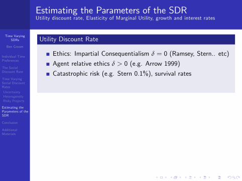
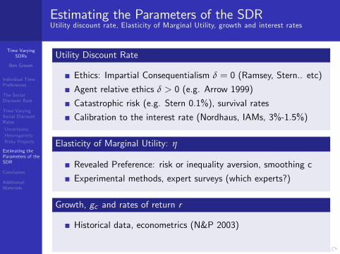
Estimating the Parameters of the SDRUtility discount rate, Elasticity of Marginal Utility, growth and interest rates
Utility Discount Rate
Ethics: Impartial Consequentialism δ = 0 (Ramsey, Stern.. etc)
Agent relative ethics δ > 0 (e.g. Arrow 1999)
Catastrophic risk (e.g. Stern 0.1%), survival rates
Calibration to the interest rate (Nordhaus, IAMs, 3%-1.5%)
Elasticity of Marginal Utility: η
Revealed Preference: risk or inequality aversion, smoothing c
Experimental methods, expert surveys (which experts?)
Growth, gc and rates of return r
Historical data, econometrics (N&P 2003)
Expert surveys (Drupp et al. 2015, Pindyck 2017)
Time VaryingSDRs
Ben Groom
Individual TimePreferences
The SocialDiscount Rate
Time VaryingSocial DiscountRates
UncertaintyHeterogeneityRisky Projects
Estimating theParameters of theSDR
Conclusion
AdditionalMaterials
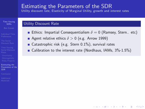
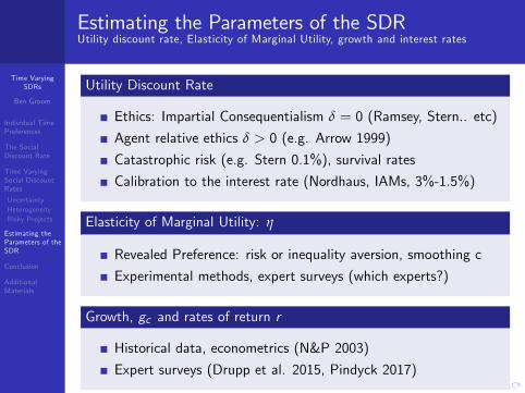
Estimating the Parameters of the SDRUtility discount rate, Elasticity of Marginal Utility, growth and interest rates
Utility Discount Rate
Ethics: Impartial Consequentialism δ = 0 (Ramsey, Stern.. etc)
Agent relative ethics δ > 0 (e.g. Arrow 1999)
Catastrophic risk (e.g. Stern 0.1%), survival rates
Calibration to the interest rate (Nordhaus, IAMs, 3%-1.5%)
Elasticity of Marginal Utility: η
Revealed Preference: risk or inequality aversion, smoothing c
Experimental methods, expert surveys (which experts?)
Growth, gc and rates of return r
Historical data, econometrics (N&P 2003)
Expert surveys (Drupp et al. 2015, Pindyck 2017)
Time VaryingSDRs
Ben Groom
Individual TimePreferences
The SocialDiscount Rate
Time VaryingSocial DiscountRates
UncertaintyHeterogeneityRisky Projects
Estimating theParameters of theSDR
Conclusion
AdditionalMaterials
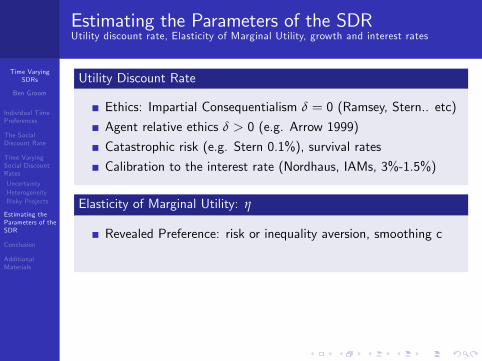
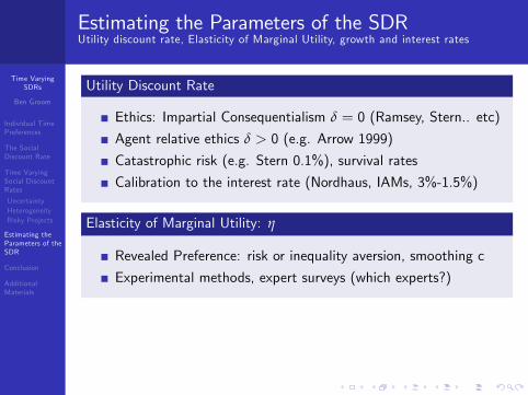
Estimating the Parameters of the SDRUtility discount rate, Elasticity of Marginal Utility, growth and interest rates
Utility Discount Rate
Ethics: Impartial Consequentialism δ = 0 (Ramsey, Stern.. etc)
Agent relative ethics δ > 0 (e.g. Arrow 1999)
Catastrophic risk (e.g. Stern 0.1%), survival rates
Calibration to the interest rate (Nordhaus, IAMs, 3%-1.5%)
Elasticity of Marginal Utility: η
Revealed Preference: risk or inequality aversion, smoothing c
Experimental methods, expert surveys (which experts?)
Growth, gc and rates of return r
Historical data, econometrics (N&P 2003)
Expert surveys (Drupp et al. 2015, Pindyck 2017)

Time VaryingSDRs
Ben Groom
Individual TimePreferences
The SocialDiscount Rate
Time VaryingSocial DiscountRates
UncertaintyHeterogeneityRisky Projects
Estimating theParameters of theSDR
Conclusion
AdditionalMaterials
Estimating the Parameters of the SDRUtility discount rate, Elasticity of Marginal Utility, growth and interest rates
Utility Discount Rate
Ethics: Impartial Consequentialism δ = 0 (Ramsey, Stern.. etc)
Agent relative ethics δ > 0 (e.g. Arrow 1999)
Catastrophic risk (e.g. Stern 0.1%), survival rates
Calibration to the interest rate (Nordhaus, IAMs, 3%-1.5%)
Elasticity of Marginal Utility: η
Revealed Preference: risk or inequality aversion, smoothing c
Experimental methods, expert surveys (which experts?)
Growth, gc and rates of return r
Historical data, econometrics (N&P 2003)
Expert surveys (Drupp et al. 2015, Pindyck 2017)
Time VaryingSDRs
Ben Groom
Individual TimePreferences
The SocialDiscount Rate
Time VaryingSocial DiscountRates
UncertaintyHeterogeneityRisky Projects
Estimating theParameters of theSDR
Conclusion
AdditionalMaterials
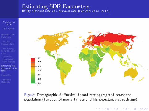
Estimating SDR ParametersUtility discount rate as a survival rate (Fenichel et al. 2017)
Figure: Demographic δ : Survival hazard rate aggregated across thepopulation (Function of mortality rate and life expectancy at each age)
Time VaryingSDRs
Ben Groom
Individual TimePreferences
The SocialDiscount Rate
Time VaryingSocial DiscountRates
UncertaintyHeterogeneityRisky Projects
Estimating theParameters of theSDR
Conclusion
AdditionalMaterials
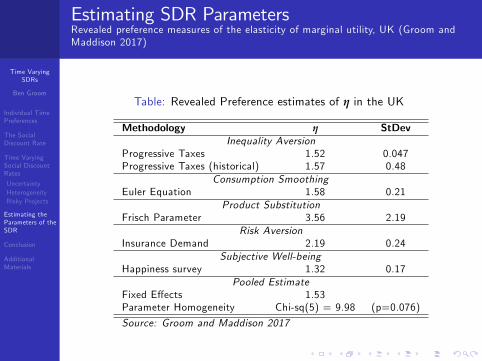
Estimating SDR ParametersRevealed preference measures of the elasticity of marginal utility, UK (Groom andMaddison 2017)
Table: Revealed Preference estimates of η in the UK
Methodology η StDevInequality Aversion
Progressive Taxes 1.52 0.047Progressive Taxes (historical) 1.57 0.48
Consumption SmoothingEuler Equation 1.58 0.21
Product SubstitutionFrisch Parameter 3.56 2.19
Risk AversionInsurance Demand 2.19 0.24
Subjective Well-beingHappiness survey 1.32 0.17
Pooled EstimateFixed E¤ects 1.53Parameter Homogeneity Chi-sq(5) = 9.98 (p=0.076)
Source: Groom and Maddison 2017
Time VaryingSDRs
Ben Groom
Individual TimePreferences
The SocialDiscount Rate
Time VaryingSocial DiscountRates
UncertaintyHeterogeneityRisky Projects
Estimating theParameters of theSDR
Conclusion
AdditionalMaterials
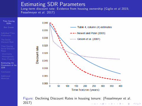
Estimating SDR ParametersLong-term discount rate: Evidence from housing ownership (Giglio et al 2015;Fesselmeyer et al. 2017)
Figure: Declining Discount Rates in housing tenure: (Fesselmeyer et al.2017)

Time VaryingSDRs
Ben Groom
Individual TimePreferences
The SocialDiscount Rate
Time VaryingSocial DiscountRates
UncertaintyHeterogeneityRisky Projects
Estimating theParameters of theSDR
Conclusion
AdditionalMaterials
Project BetasFrench Guidelines (Gollier 2011)
Sector Estimatedconsumption
BetaAgriculture, Silviculture and Fisheries 0.85Industry 2.09
Automobile Industry 4.98Manufacture of Mechanical Equipment 3.00
Intermediate Industries 2.76Energy 0.85
Construction 1,45Transport 1.60Administrative Services 0.09
Education 0.11Health 0.24
Financial Services 0.15Financial Intermediation 0.49
Assurance 0.36
Time VaryingSDRs
Ben Groom
Individual TimePreferences
The SocialDiscount Rate
Time VaryingSocial DiscountRates
UncertaintyHeterogeneityRisky Projects
Estimating theParameters of theSDR
Conclusion
AdditionalMaterials
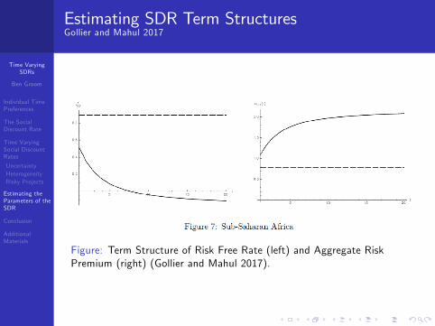
Estimating SDR Term StructuresGollier and Mahul 2017
Figure: Term Structure of Risk Free Rate (left) and Aggregate RiskPremium (right) (Gollier and Mahul 2017).
Time VaryingSDRs
Ben Groom
Individual TimePreferences
The SocialDiscount Rate
Time VaryingSocial DiscountRates
UncertaintyHeterogeneityRisky Projects
Estimating theParameters of theSDR
Conclusion
AdditionalMaterials
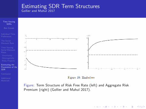
Estimating SDR Term StructuresGollier and Mahul 2017
Figure: Term Structure of Risk Free Rate (left) and Aggregate RiskPremium (right) (Gollier and Mahul 2017).
Time VaryingSDRs
Ben Groom
Individual TimePreferences
The SocialDiscount Rate
Time VaryingSocial DiscountRates
UncertaintyHeterogeneityRisky Projects
Estimating theParameters of theSDR
Conclusion
AdditionalMaterials
ConclusionProject Appraisal in LMICs
Declining Discount Rates for risk free projects
TVSDRs? Empirics: persistence? variability? risk prefs?
Prudence and high variability: large prudence e¤ects
Low growth, low SDR: Liberia, DRC, (-2%) etc.
High growth, high SDR: Botswana, South Africa (+4%), etc
Risky Projects
Term structure for risky projects depends on the �beta�
Risk premium rises with the time horizon for β > 0
Practical Advice
SDR important (country speci�c), but so is valuation
Empirical work exists to help guide decision makers
Time VaryingSDRs
Ben Groom
Individual TimePreferences
The SocialDiscount Rate
Time VaryingSocial DiscountRates
UncertaintyHeterogeneityRisky Projects
Estimating theParameters of theSDR
Conclusion
AdditionalMaterials
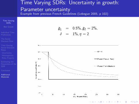
Time Varying SDRs: Uncertainty in growth:Parameter uncertaintyExample from previous French Guidelines (Lebegue 2005, p 102)
g1 = 0.5%, g2 = 2%,
δ = 1%, η = 2
Time VaryingSDRs
Ben Groom
Individual TimePreferences
The SocialDiscount Rate
Time VaryingSocial DiscountRates
UncertaintyHeterogeneityRisky Projects
Estimating theParameters of theSDR
Conclusion
AdditionalMaterials
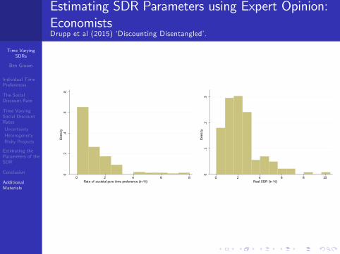
Estimating SDR Parameters using Expert Opinion:EconomistsDrupp et al (2015) �Discounting Disentangled�.
0.2
.4.6
.8De
nsity
0 2 4 6 8Rate of societal pure time preference (in %)
0.1
.2.3
Dens
ity
0 2 4 6 8 10Real SDR (in %)
Time VaryingSDRs
Ben Groom
Individual TimePreferences
The SocialDiscount Rate
Time VaryingSocial DiscountRates
UncertaintyHeterogeneityRisky Projects
Estimating theParameters of theSDR
Conclusion
AdditionalMaterials
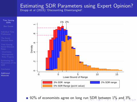
Estimating SDR Parameters using Expert Opinion?Drupp et al (2015) �Discounting Disentangled�.
1% 2%
0.2
.4.6
.81
Den
sity
5 0 5 10 15Lower Bound of Range
3% SDR range 2% SDR range0% SDR Range (point value)
92% of economists agree on long run SDR between 1% and 3%
Time VaryingSDRs
Ben Groom
Individual TimePreferences
The SocialDiscount Rate
Time VaryingSocial DiscountRates
UncertaintyHeterogeneityRisky Projects
Estimating theParameters of theSDR
Conclusion
AdditionalMaterials
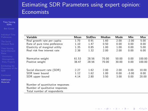
Estimating SDR Parameters using expert opinion:Economists
Variable Mean StdDev Median Mode Min Max NReal growth rate per capita 1.70 0.91 1.60 2.00 -2.00 5.00 181Rate of pure time preference 1.10 1.47 0.50 0.00 0.00 8.00 180Elasticity of marginal utility 1.35 0.85 1.00 1.00 0.00 5.00 173Real risk free interest rate 2.38 1.32 2.00 2.00 0.00 6.00 176
Normative weight 61.53 28.56 70.00 50.00 0.00 100.00 182Positive weight 38.47 28.56 70.00 30.00 0.00 100.00 182
Social discount rate (SDR) 2.27 1.62 2.00 2.00 0.00 10.00 181SDR lower bound 1.12 1.62 1.00 0.00 -3.00 8.00 182SDR upper bound 4.14 2.80 3.50 3.00 0.00 20.00 183
Number of quantitative responses 185Number of qualitative responses 99Total number of respondents 197
Time VaryingSDRs
Ben Groom
Individual TimePreferences
The SocialDiscount Rate
Time VaryingSocial DiscountRates
UncertaintyHeterogeneityRisky Projects
Estimating theParameters of theSDR
Conclusion
AdditionalMaterials
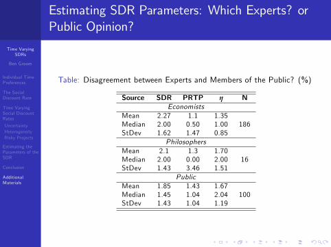
Estimating SDR Parameters: Which Experts? orPublic Opinion?
Table: Disagreement between Experts and Members of the Public? (%)
Source SDR PRTP η NEconomists
Mean 2.27 1.1 1.35Median 2.00 0.50 1.00 186StDev 1.62 1.47 0.85
PhilosophersMean 2.1 1.3 1.70Median 2.00 0.00 2.00 16StDev 1.43 3.46 1.51
PublicMean 1.85 1.43 1.67Median 1.45 1.04 2.04 100StDev 1.43 1.04 1.19
Time VaryingSDRs
Ben Groom
Individual TimePreferences
The SocialDiscount Rate
Time VaryingSocial DiscountRates
UncertaintyHeterogeneityRisky Projects
Estimating theParameters of theSDR
Conclusion
AdditionalMaterials
Social Discounting: References
Cropper, M.,Freeman,M.,Groom,B.,Pizer,W.,2014.Decliningdiscount rates.Am.Econ.Rev.:Pap.Proc.104,538�543.Drupp, M.A., Freeman,M.C. ,Groom,B., Nesje,F., 2015.Discounting Disentangled: An Expert Survey on theDeterminants of the Long-Term Social Discount Rate.Grantham Research Institute Working Paper No.172. LondonSchool of Economics.Fenichel et al (2017). Even the representative agent must die!....NBER Working Paper No. w23591Freeman,M.C.,Groom,B.,2015. Positively gamma discounting:combining the opinions of experts on the social discount rate.Econ.J. 125,1015�1024.Freeman, et al, 2015. Declining discount rates and the FisherE¤ect: in�ated past, discounted future? Journal ofEnvironmental Economics and Management, 73, pp. 32-39Gollier, C., 2012. Pricing the Planet�s Future: The Economics ofDiscounting in an Uncertain World. Princeton University Press,Princeton.
Time VaryingSDRs
Ben Groom
Individual TimePreferences
The SocialDiscount Rate
Time VaryingSocial DiscountRates
UncertaintyHeterogeneityRisky Projects
Estimating theParameters of theSDR
Conclusion
AdditionalMaterials
Social Discounting: References
Gollier, Christian. 2013. �Evaluation of Long-Dated InvestmentsUnder Uncertain Growth Trend, Volatility and Catastrophes.�Toulouse School of Economics TSE Working Papers 12-361.
Gollier, Christian. 2012b. Term Structures of discount rates forrisky investments IDEI, mimeo.
Groom B and Hepburn C (2017). Looking back at SocialDiscount Rates..... Review of Environmental Economics andPolicy, Volume 11, Issue 2, 1 July 2017, Pages 336�356,https://doi.org/10.1093/reep/rex015
Groom, B., Maddison,D.J. ,2013. Non-Identical Quadruplets:Four New Estimates of the Elasticity of Marginal Utility for theUK. Grantham Institute Centre for Climate Change Economicsand Policy Working Paper No.141.
Harberger A.C. and Jenkins G (2015). Musings on the SocialDiscount Rate. Journal of bene�t-cost analysis, Vol. 6.2015, 1,p. 6-32
Time VaryingSDRs
Ben Groom
Individual TimePreferences
The SocialDiscount Rate
Time VaryingSocial DiscountRates
UncertaintyHeterogeneityRisky Projects
Estimating theParameters of theSDR
Conclusion
AdditionalMaterials
Social Discounting: References
Heal,G. and Millner, A.,2014. Agreeing to disagree on climatepolicy. Proc. Natl. Acad. Sci. 111, 3695�3698.
Moore et al (2013). More Appropriate Social Discounting.....Journal of Bene�t-Cost Analysis, 2013, vol. 4, issue 1, 1-16
Newell R and Pizer W (2003). Discounting the bene�ts ofclimate change: How much do uncertain interest rates increasevaluations? Journal of Environmental Economics andManagement, 46(1), 52-74.
Weitzman,M.L.,1998.Why the far-distant future should bediscounted at its lowest possible rate.J.Environ.Econ.Manag.36,201�208.
Weitzman,M.L.,2001.Gamma discounting.Am.Econ.Rev.91,260�271.
Related Documents