Discounted Cash Flow Valuation. Challenges Defining and forecasting CF’s Estimating appropriate discount rate.

Discounted Cash Flow Valuation

Challenges

Defining and forecasting CF’s

Estimating appropriate discount rate

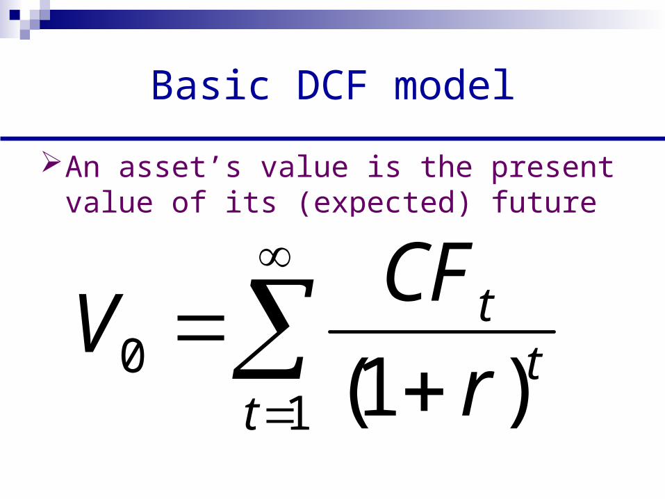
Basic DCF model

An asset’s value is the present value of its (expected) future cash flows

10 )1(t

tt

r

CFV

Three alternative definitions of cash flow

Dividend discount model

Free cash flow model

Residual income model

Free cash flow

Free cash flow to the firm (FCFF) is cash flow from operations minus capital expenditures

Free cash flow to equity (FCFE) is cash flow from operations minus capital expenditures minus net payments to debtholders (interest and principal)

FCF valuation

PV of FCFF is the total value of the company. Value of equity is PV of FCFF minus the market value of outstanding debt.

PV of FCFE is the value of equity.

Discount rate for FCFF is the WACC. Discount rate for FCFE is the cost of equity (required rate of return for equity).

Intro to Free Cash Flows

Dividends are the cash flows actually paid to stockholders

Free cash flows are the cash flows available for distribution.

Defining Free Cash Flow

Free cash flow to equity (FCFE) is the cash flow available to the firm’s common equity holders after all operating expenses, interest and principal payments have been paid, and necessary investments in working and fixed capital have been made.

• FCFE is the cash flow from operations minus capital expenditures minus payments to (and plus receipts from) debtholders.

Valuing FCFE

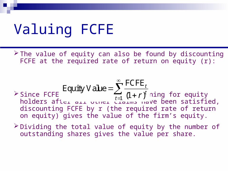
The value of equity can also be found by discounting FCFE at the required rate of return on equity (r):

Since FCFE is the cash flow remaining for equity holders after all other claims have been satisfied, discounting FCFE by r (the required rate of return on equity) gives the value of the firm’s equity.

Dividing the total value of equity by the number of outstanding shares gives the value per share.

1

FCFEEquity Value

(1 )tt

t r

Discount rate determination

Jargon

• Discount rate: any rate used in finding the present value of a future cash flow

• Risk premium: compensation for risk, measured relative to the risk-free rate

• Required rate of return: minimum return required by investor to invest in an asset

• Cost of equity: required rate of return on common stock

Two major approaches for cost of equity

Equilibrium models:

• Capital asset pricing model (CAPM)

• Arbitrage pricing theory (APT)

Bond yield plus risk premium method (BYPRP)

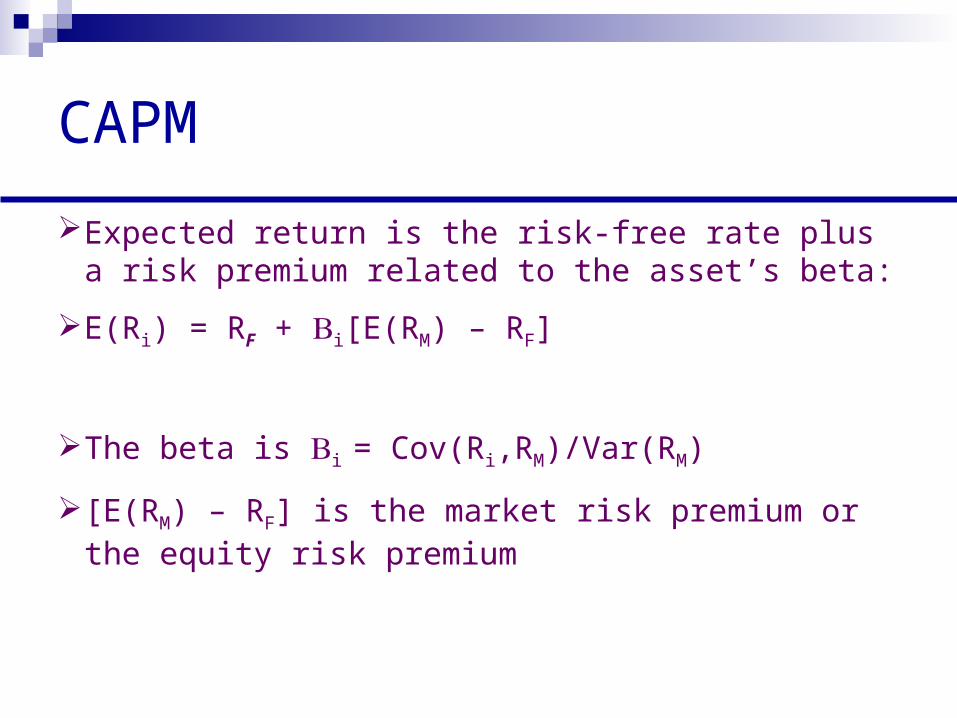
CAPM

Expected return is the risk-free rate plus a risk premium related to the asset’s beta:

E(Ri) = RF + i[E(RM) – RF]

The beta is i = Cov(Ri,RM)/Var(RM)

[E(RM) – RF] is the market risk premium or the equity risk premium

CAPM

What do we use for the risk-free rate of return?

• Choice is often a short-term rate such as the 30-day T-bill rate or a long-term government bond rate.

• We usually match the duration of the bond rate with the investment period, so we use the long-term government bond rate.

• Risk-free rate must be coordinated with how the equity risk premium is calculated (i.e., both based on same bond maturity).

Equity risk premium

Historical estimates: Average difference between equity market returns and government debt returns.

• Choice between arithmetic mean return or geometric mean return

• Survivorship bias

• ERP varies over time

• ERP differs in different markets

Equity risk premium

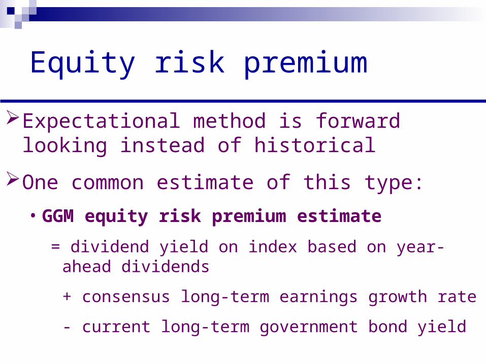
Expectational method is forward looking instead of historical

One common estimate of this type:

• GGM equity risk premium estimate

= dividend yield on index based on year-ahead dividends

+ consensus long-term earnings growth rate

- current long-term government bond yield

Sources of error in using models

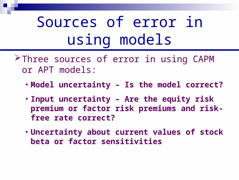
Three sources of error in using CAPM or APT models:

• Model uncertainty – Is the model correct?

• Input uncertainty – Are the equity risk premium or factor risk premiums and risk-free rate correct?

• Uncertainty about current values of stock beta or factor sensitivities

BYPRP method

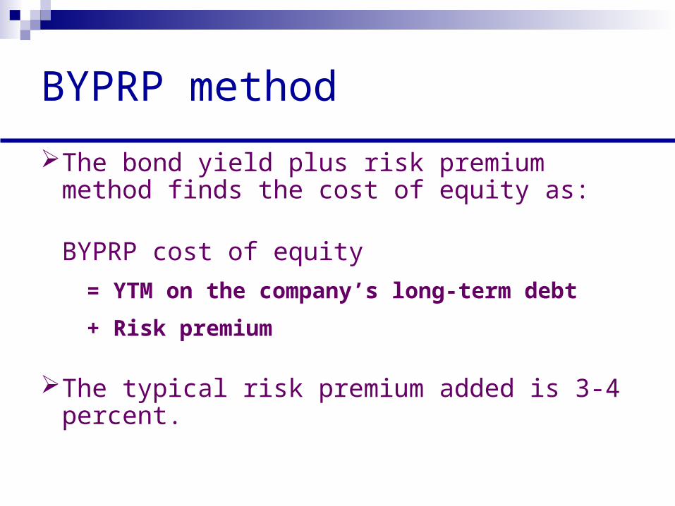
The bond yield plus risk premium method finds the cost of equity as:

BYPRP cost of equity

= YTM on the company’s long-term debt

+ Risk premium

The typical risk premium added is 3-4 percent.

Single-stage, constant-growth FCFE valuation model

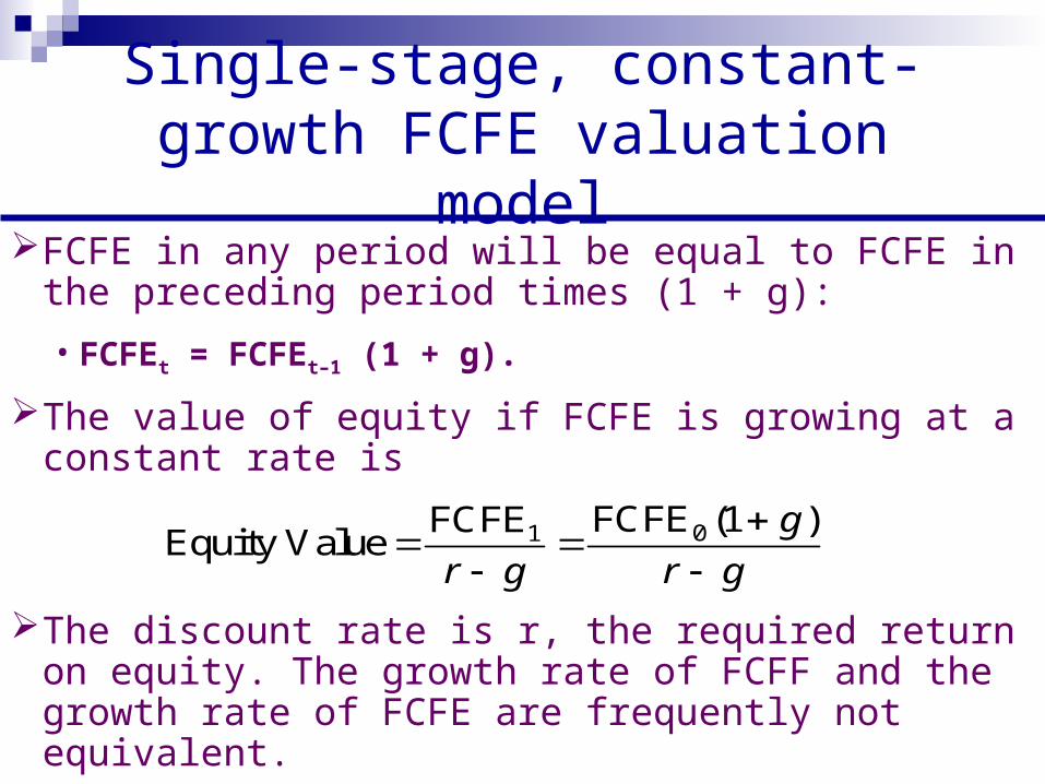
FCFE in any period will be equal to FCFE in the preceding period times (1 + g):

• FCFEt = FCFEt–1 (1 + g).

The value of equity if FCFE is growing at a constant rate is

The discount rate is r, the required return on equity. The growth rate of FCFF and the growth rate of FCFE are frequently not equivalent.

01 FCFE (1 )FCFEEquity Value

g

r g r g

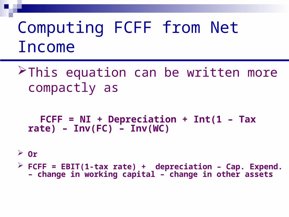
Computing FCFF from Net Income

This equation can be written more compactly as

FCFF = NI + Depreciation + Int(1 – Tax rate) – Inv(FC) – Inv(WC)

Or

FCFF = EBIT(1-tax rate) + depreciation – Cap. Expend. – change in working capital – change in other assets

Forecasting free cash flows

Computing FCFF and FCFE based upon historical accounting data is straightforward. Often times, this data is then used directly in a single-stage DCF valuation model.

On other occasions, the analyst desires to forecast future FCFF or FCFE directly. In this case, the analyst must forecast the individual components of free cash flow. This section extends our previous presentation on computing FCFF and FCFE to the more complex task of forecasting FCFF and FCFE. We present FCFF and FCFE valuation models in the next section.

Forecasting free cash flows

Given that we have a variety of ways in which to derive free cash flow on a historical basis, it should come as no surprise that there are several methods of forecasting free cash flow.

One approach is to compute historical free cash flow and apply some constant growth rate. This approach would be appropriate if free cash flow for the firm tended to grow at a constant rate and if historical relationships between free cash flow and fundamental factors were expected to be maintained.

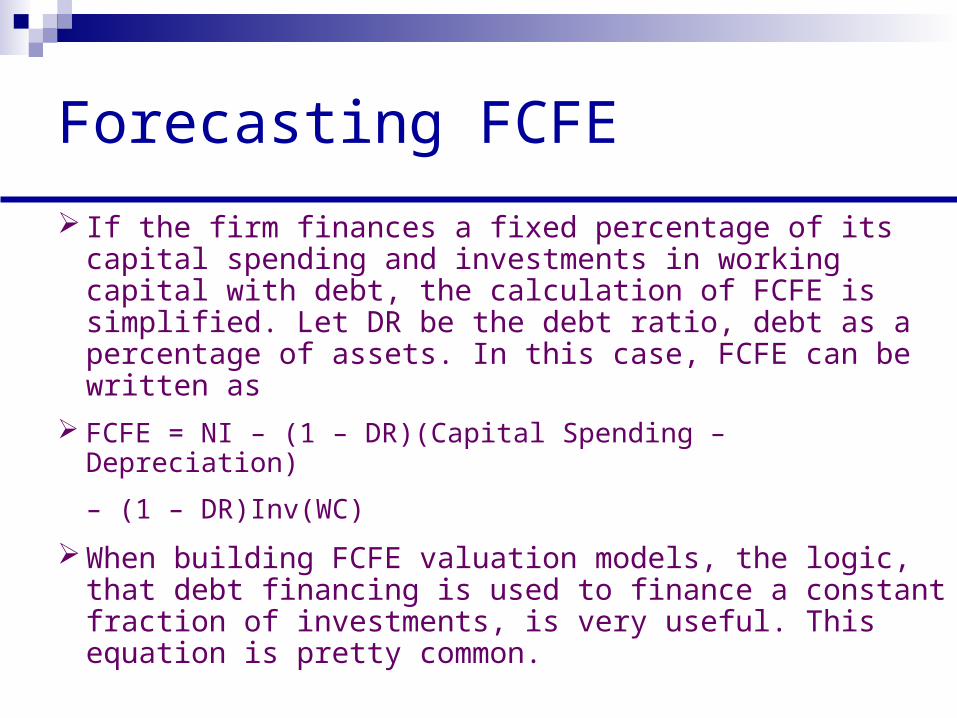
Forecasting FCFE

If the firm finances a fixed percentage of its capital spending and investments in working capital with debt, the calculation of FCFE is simplified. Let DR be the debt ratio, debt as a percentage of assets. In this case, FCFE can be written as

FCFE = NI – (1 – DR)(Capital Spending – Depreciation)

– (1 – DR)Inv(WC)

When building FCFE valuation models, the logic, that debt financing is used to finance a constant fraction of investments, is very useful. This equation is pretty common.

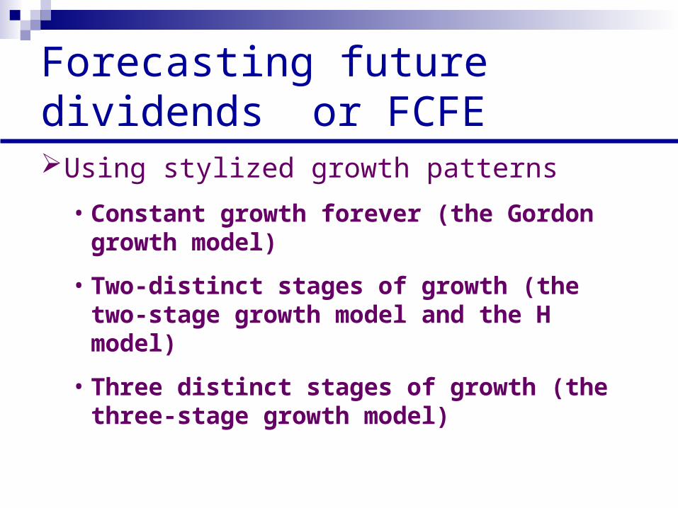
Forecasting future dividends or FCFEUsing stylized growth patterns

• Constant growth forever (the Gordon growth model)

• Two-distinct stages of growth (the two-stage growth model and the H model)

• Three distinct stages of growth (the three-stage growth model)

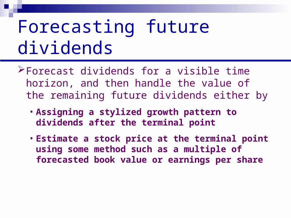
Forecasting future dividends

Forecast dividends for a visible time horizon, and then handle the value of the remaining future dividends either by

• Assigning a stylized growth pattern to dividends after the terminal point

• Estimate a stock price at the terminal point using some method such as a multiple of forecasted book value or earnings per share

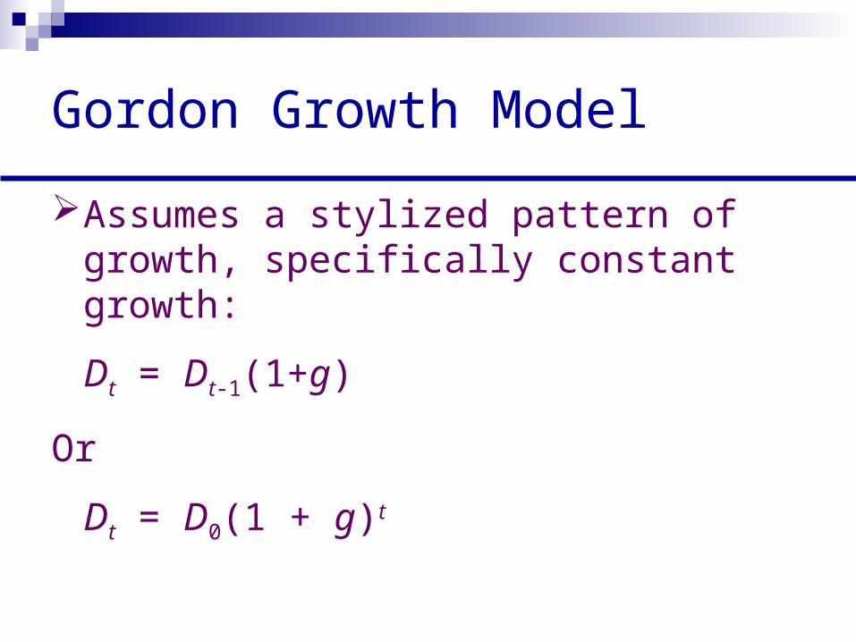
Gordon Growth Model

Assumes a stylized pattern of growth, specifically constant growth:

Dt = Dt-1(1+g)

Or

Dt = D0(1 + g)t

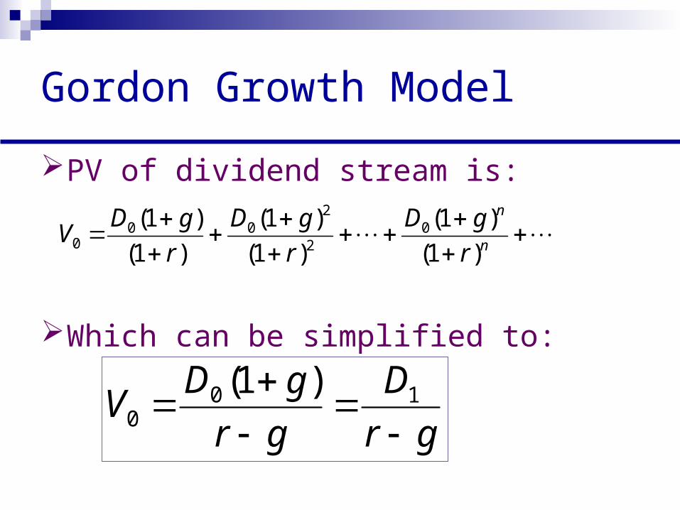
Gordon Growth Model

PV of dividend stream is:

Which can be simplified to:

n

n

r

gD

r

gD

r

gDV

)1(

)1(

)1(

)1(

)1(

)1( 02

200

0

gr

D

gr

gDV

100

)1(

Gordon growth model

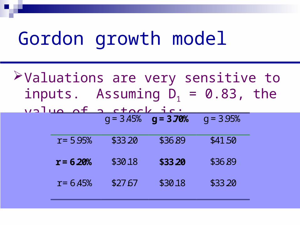
Valuations are very sensitive to inputs. Assuming D1 = 0.83, the value of a stock is:

g = 3.45% g = 3.70% g = 3.95%

r = 5.95% $33.20 $36.89 $41.50

r = 6.20% $30.18 $33.20 $36.89

r = 6.45% $27.67 $30.18 $33.20

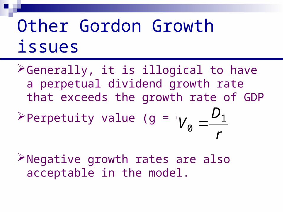
Other Gordon Growth issues

Generally, it is illogical to have a perpetual dividend growth rate that exceeds the growth rate of GDP

Perpetuity value (g = 0):

Negative growth rates are also acceptable in the model.

r

DV 1

0

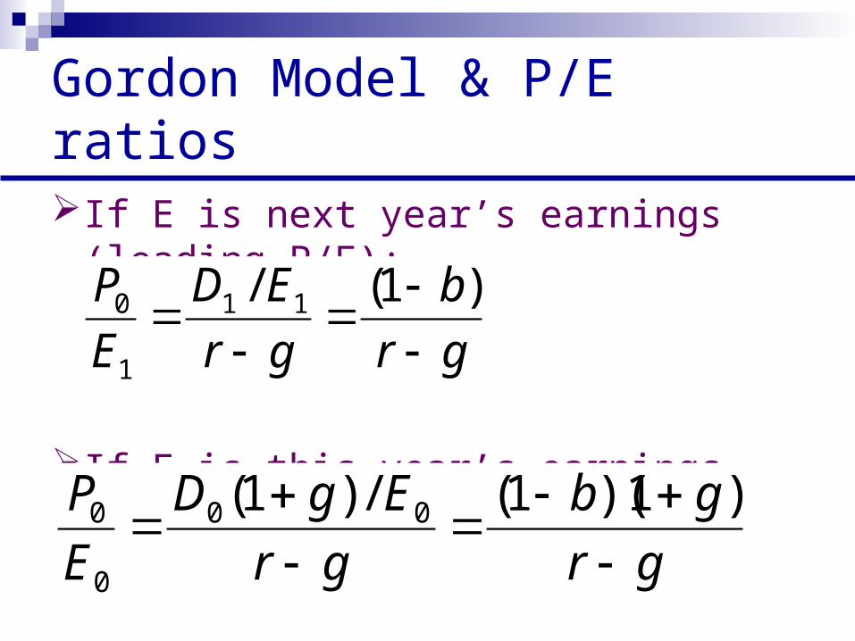
Gordon Model & P/E ratios

If E is next year’s earnings (leading P/E):

If E is this year’s earnings (trailing P/E):

gr

b

gr

ED

E

P

)1(/ 11

1

0

gr

gb

gr

EgD

E

P

)1)(1(/)1( 00

0

0

Using a P/E for terminal value

The terminal value at the beginning of the second stage was found above with a Gordon growth model, assuming a long-term sustainable growth rate.

The terminal value can also be found using another method to estimate the terminal value at t = n. You can also use a P/E ratio, applied to estimated earnings at t = n.

Using a P/E for terminal value

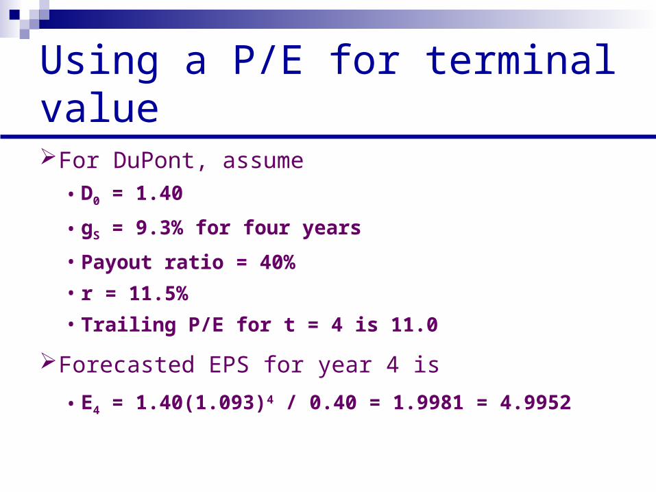
For DuPont, assume

• D0 = 1.40

• gS = 9.3% for four years

• Payout ratio = 40%

• r = 11.5%

• Trailing P/E for t = 4 is 11.0

Forecasted EPS for year 4 is

• E4 = 1.40(1.093)4 / 0.40 = 1.9981 = 4.9952

Using a P/E for terminal value

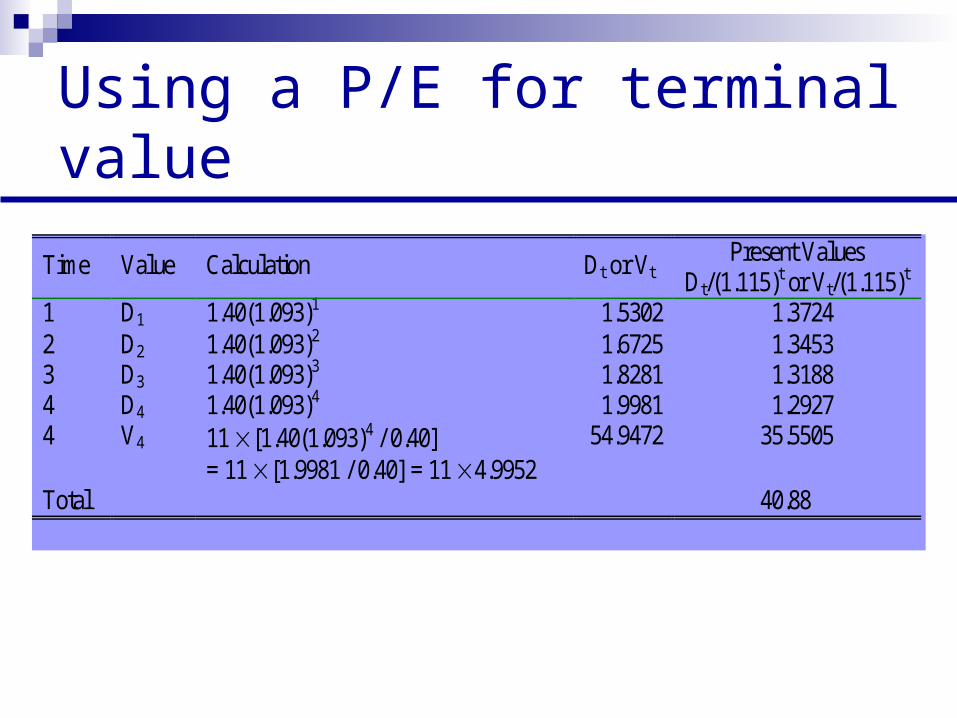
Time Value Calculation Dt or Vt Present Values

Dt/(1.115)t or Vt/(1.115)t 1 D1 1.40(1.093)1 1.5302 1.3724 2 D2 1.40(1.093)2 1.6725 1.3453 3 D3 1.40(1.093)3 1.8281 1.3188 4 D4 1.40(1.093)4 1.9981 1.2927 4 V4 11 [1.40(1.093)4 / 0.40]

= 11 [1.9981 / 0.40] = 11 4.9952 54.9472 35.5505

Total 40.88

Three-stage DDM

There are two popular version of the three-stage DDM• The first version is like the two-stage model, only the

firm is assumed to have a constant dividend growth rate in each of the three stages.

• A second version of the three-stage DDM combines the two-stage DDM and the H model. In the first stage, dividends grow at a high, constant (supernormal) rate for the whole period. In the second stage, dividends decline linearly as they do in the H model. Finally, in stage three, dividends grow at a sustainable, constant rate.

Spreadsheet modeling

Spreadsheets allow the analyst to build very complicated models that would be very cumbersome to describe using algebra.

Built-in functions such as those to find rates of return use algorithms to get a numerical answer when a mathematical solution would be impossible or extremely

complicated.

Strengths of multistage DDMs

Can accommodate a variety of patterns of future dividend streams.

Even though they may not replicate the future dividends exactly, they can be a useful approximation.

The expected rates of return can be imputed by finding the discount rate that equates the present value of the dividend stream to the current stock price.

Strengths of multistage DDMs

Because of the variety of DDMs available, the analyst is both enabled and compelled to evaluate carefully the assumptions about the stock under examination.

Spreadsheets are widely available, allowing the analyst to construct and solve an almost limitless number of models.

Weaknesses of multistage DDMs

Garbage in, garbage out. If the inputs are not economically meaningful, the outputs from the model will be of questionable value.

Analysts sometimes employ models that they do not understand fully.

Valuations are very sensitive to the inputs to the models.

Forecasting growth rates

There are three basic methods for forecasting growth rates:

• Using analyst forecasts

• Using historical rates (use historical dividend growth rate or use a statistical forecasting model based on historical data)

• Using company and industry fundamentals

Finding g

The simplest model of the dividend growth rate is:

• g = b x ROE

• where g = Dividend growth rate

• b = Earnings retention rate (1 – payout ratio)

• ROE = Return on equity.