Disappointment Aversion Preferences in General Equilibrium ...

Great Expectations, Greater Disappointment:Disappointment Aversion Preferences in General

Equilibrium Asset Pricing Models

by

Stefanos Delikouras

A dissertation submitted in partial fulfillmentof the requirements for the degree of

Doctor of Philosophy(Business Administration)

in The University of Michigan2013

Doctoral Committee:

Associate Professor Robert F. Dittmar, ChairProfessor Miles S. KimballProfessor Reuven LehavyAssociate Professor Paolo PasquarielloProfessor Tyler G. Shumway

Σα βγεις στoν πηγαιµo για την Iθακη, On your way to Ithaka, you should hope

να ευχεσαι να ‘ναι µακρυς o δρoµoς, that there lies a long journey ahead of you,

γεµατoς περιπετειες, γεµατoς γνωσεις. full of adventures, full of knowledge.

Toυς Λαιστρυγoνας και τoυς Kυκλωπας, Of the Lestrygonians and the Cyclops,

τoν θυµωµενo Πoσειδωνα µη φoβασαι of the angry Poseidon, have no fear

extract from the poem “Ithaca” by Constantine P. Cavafy (1863-1933)

Odysseus and the cyclops Polyphemus by Arnold Bocklin (1827-1902). 1896. Oil on panel.

75.5 x 148.5 cm. Private collection

c© Stefanos Delikouras 2013

All Rights Reserved

To my beloved family, Nickolaos, Eleni and Eirini. I could have never come thus far

without your unconditional encouragement, love, and support over the years.

To Lavrentia, my only reason for undertaking and completing this journey.

ii

ACKNOWLEDGEMENTS

This dissertation could not have been completed, had it not been for so many

people. First and foremost, I am grateful to Robert Dittmar, my doctoral committee

chair, whom I first met almost ten years ago when I was a student at the Financial

Engineering program. His contribution to my Doctorate degree has been crucial long

before this journey even began. Had it not been for his recommendation letter, it

would have been difficult for me to get accepted into the Doctoral program at the Ross

School of Business. Robert has been a catalyst in my academic development from a

PhD student to a young scholar. Besides the numerous research opportunities he has

given me through our co-authored papers, he has always taken a sincere interest on

my research agenda, and has spent a lot of time providing me with valuable feedback

on my research endeavors.

I am particularly grateful to Paolo Pasquariello, whom I also met while being a

student at the Financial Engineering program, for his help and support. His advice

has been critical in improving my presentation skills, and successfully navigating

through the job market. Moreover, during my teaching semester, Paolo’s suggestions

were indispensable in assembling a novel curriculum for the undergraduate course in

International Finance.

I would like to thank Tyler Shumway because his behavioral finance class inspired

me to introduce elements of behavioral economics in my orthodox view of a ratio-

nal world. I am also grateful to Francisco Palomino who taught me the basic tools

for solving dynamic stochastic general equilibrium models with non-separable pref-

iii

erences. This dissertation is actually based on a term project for Francisco’s special

topics class. Finally, I owe Miles Kimball a huge part of my economics background,

and I would like to thank him for teaching me how to communicate finance concepts

to an economic audience.

I would also like to thank Sugato Battacharrya, Mattias Cattaneo, Joseph Con-

lon, Amy Dittmar, Lutz Kilian, Reuven Lehavy, NP Narayanan, Amiyatosh Purnan-

dadam, Uday Rajan, and Lu Zhang for their time, attention, and research discussions

during the last five years. My research profile would not be the same if it weren’t

for all these wonderful scholars who helped shape my academic personality. Finally,

I would like to thank Achilleas Anastasopoulos, Samir Nurmohamed, Robert Smith,

and Daniel Weagley for their support and advice. Special thanks to all the people

who put together a nice LATEX template for me to use for my dissertation, and to

Alex Hsu for letting me know that such a template exists.

iv

PREFACE

Two years ago, during the weekly finance seminar at Ross, I was having lunch

with a well-known scholar in the field of asset pricing. When I asked him whether it

would be possible to introduce a stochastic discount factor based on a “habit model”

with forward-looking reference levels, he immediately replied that such a model would

be really hard to solve.

For the following year I was trying to wrap my head around the problem of intro-

ducing preferences with expectation-based reference levels into asset pricing models.

Unfortunately, Gul had already done that back in 1991 when he introduced disap-

pointment aversion preferences. Disappointment aversion relies on the simple and

intuitive fact that people feel really sad whenever things turn out worse than ex-

pected. Although the theoretical framework for expectation-based utility functions

was established more than twenty years ago, disappointment aversion preferences have

been largely overlooked in favor of Kahneman’s and Tversky’s (1979) loss aversion

model.

Disappointment aversion preferences combine well established behavioral patterns

for decision making under uncertainty, such as reference-based utility and asymmet-

ric marginal utility, with a number of economically tractable properties. For in-

stance, unlike most behavioral models, disappointment aversion preferences do not

violate first-order stochastic dominance, transitivity of preferences or aggregation of

investors, and can therefore help us shed additional light on the link between financial

markets and aggregate economic activity, while maintaining investor rationality.

v

TABLE OF CONTENTS

DEDICATION . . . . . . . . . . . . . . . . . . . . . . . . . . . . . . . . . . ii

ACKNOWLEDGEMENTS . . . . . . . . . . . . . . . . . . . . . . . . . . iii

PREFACE . . . . . . . . . . . . . . . . . . . . . . . . . . . . . . . . . . . . . v

LIST OF FIGURES . . . . . . . . . . . . . . . . . . . . . . . . . . . . . . . viii

LIST OF TABLES . . . . . . . . . . . . . . . . . . . . . . . . . . . . . . . . ix

LIST OF APPENDICES . . . . . . . . . . . . . . . . . . . . . . . . . . . . x

LIST OF ABBREVIATIONS . . . . . . . . . . . . . . . . . . . . . . . . . xi

ABSTRACT . . . . . . . . . . . . . . . . . . . . . . . . . . . . . . . . . . . xiii

CHAPTER

I. Disappointment Events in Consumption Growth, and theCross-Section of Expected Stock Returns . . . . . . . . . . . . 1

1.1 Abstract . . . . . . . . . . . . . . . . . . . . . . . . . . . . . 11.2 Introduction . . . . . . . . . . . . . . . . . . . . . . . . . . . 21.3 Recursive utility with disappointment aversion preferences . . 61.4 Estimation . . . . . . . . . . . . . . . . . . . . . . . . . . . . 151.5 Related literature . . . . . . . . . . . . . . . . . . . . . . . . 401.6 Conclusion . . . . . . . . . . . . . . . . . . . . . . . . . . . . 461.7 Tables . . . . . . . . . . . . . . . . . . . . . . . . . . . . . . . 481.8 Figures . . . . . . . . . . . . . . . . . . . . . . . . . . . . . . 56

II. Disappointment Aversion Preferences, and the Credit SpreadPuzzle . . . . . . . . . . . . . . . . . . . . . . . . . . . . . . . . . . 65

2.1 Abstract . . . . . . . . . . . . . . . . . . . . . . . . . . . . . 652.2 Introduction . . . . . . . . . . . . . . . . . . . . . . . . . . . 66

vi

2.3 The credit spread puzzle . . . . . . . . . . . . . . . . . . . . . 702.4 Recursive utility with disappointment aversion preferences . . 772.5 Simulation results for the disappointment aversion discount

factor . . . . . . . . . . . . . . . . . . . . . . . . . . . . . . . 862.6 Related literature . . . . . . . . . . . . . . . . . . . . . . . . 992.7 Conclusion . . . . . . . . . . . . . . . . . . . . . . . . . . . . 1012.8 Tables . . . . . . . . . . . . . . . . . . . . . . . . . . . . . . . 1032.9 Figures . . . . . . . . . . . . . . . . . . . . . . . . . . . . . . 111

APPENDICES . . . . . . . . . . . . . . . . . . . . . . . . . . . . . . . . . . 115

BIBLIOGRAPHY . . . . . . . . . . . . . . . . . . . . . . . . . . . . . . . . 153

vii

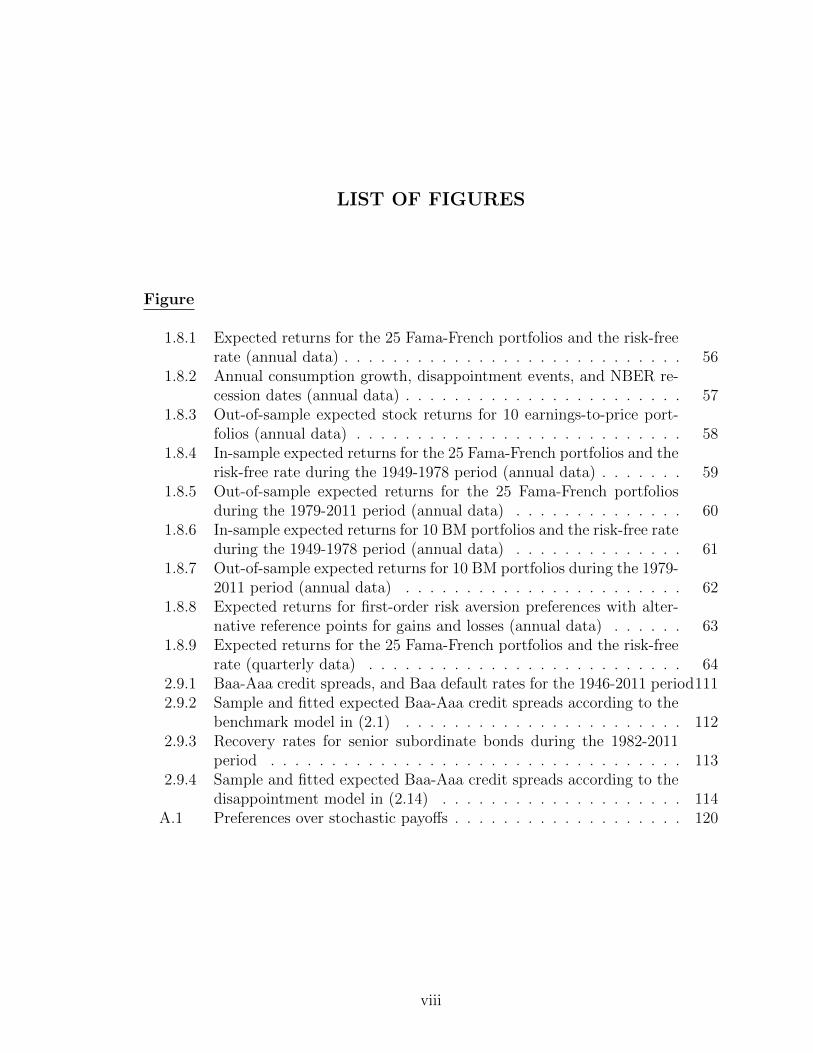
LIST OF FIGURES

Figure

1.8.1 Expected returns for the 25 Fama-French portfolios and the risk-freerate (annual data) . . . . . . . . . . . . . . . . . . . . . . . . . . . . 56

1.8.2 Annual consumption growth, disappointment events, and NBER re-cession dates (annual data) . . . . . . . . . . . . . . . . . . . . . . . 57

1.8.3 Out-of-sample expected stock returns for 10 earnings-to-price port-folios (annual data) . . . . . . . . . . . . . . . . . . . . . . . . . . . 58

1.8.4 In-sample expected returns for the 25 Fama-French portfolios and therisk-free rate during the 1949-1978 period (annual data) . . . . . . . 59

1.8.5 Out-of-sample expected returns for the 25 Fama-French portfoliosduring the 1979-2011 period (annual data) . . . . . . . . . . . . . . 60

1.8.6 In-sample expected returns for 10 BM portfolios and the risk-free rateduring the 1949-1978 period (annual data) . . . . . . . . . . . . . . 61

1.8.7 Out-of-sample expected returns for 10 BM portfolios during the 1979-2011 period (annual data) . . . . . . . . . . . . . . . . . . . . . . . 62

1.8.8 Expected returns for first-order risk aversion preferences with alter-native reference points for gains and losses (annual data) . . . . . . 63

1.8.9 Expected returns for the 25 Fama-French portfolios and the risk-freerate (quarterly data) . . . . . . . . . . . . . . . . . . . . . . . . . . 64

2.9.1 Baa-Aaa credit spreads, and Baa default rates for the 1946-2011 period1112.9.2 Sample and fitted expected Baa-Aaa credit spreads according to the

benchmark model in (2.1) . . . . . . . . . . . . . . . . . . . . . . . 1122.9.3 Recovery rates for senior subordinate bonds during the 1982-2011

period . . . . . . . . . . . . . . . . . . . . . . . . . . . . . . . . . . 1132.9.4 Sample and fitted expected Baa-Aaa credit spreads according to the

disappointment model in (2.14) . . . . . . . . . . . . . . . . . . . . 114A.1 Preferences over stochastic payoffs . . . . . . . . . . . . . . . . . . . 120

viii

LIST OF TABLES

Table

1.7.1 Summary statistics . . . . . . . . . . . . . . . . . . . . . . . . . . . 481.7.2 GMM results for the 25 Fama-French portfolios and the risk-free rate

(annual data) . . . . . . . . . . . . . . . . . . . . . . . . . . . . . . 491.7.3 NBER recessions and disappointment years (annual data) . . . . . . 501.7.4 Out-of-sample expected stock returns for 10 earnings-to-price port-

folios and the stock market (annual data) . . . . . . . . . . . . . . . 511.7.5 GMM results for the 25 Fama-French portfolios and the risk-free rate

during the 1949-1978 period (annual data) . . . . . . . . . . . . . . 521.7.6 GMM results for 10 Book-to-Market portfolios and the risk-free rate

during the 1949-1978 period (annual data) . . . . . . . . . . . . . . 531.7.7 GMM results for first-order risk aversion preferences with alternative

reference points for gains and losses (annual data) . . . . . . . . . . 541.7.8 GMM results for the 25 Fama-French portfolios and the risk-free rate

(quarterly data) . . . . . . . . . . . . . . . . . . . . . . . . . . . . . 552.8.1 Average default rates, and expected credit spreads for Baa and Aaa

bonds . . . . . . . . . . . . . . . . . . . . . . . . . . . . . . . . . . . 1032.8.2 OLS regression of recovery rates on aggregate consumption growth

(1982-2011) . . . . . . . . . . . . . . . . . . . . . . . . . . . . . . . 1042.8.3 Preference parameters, and state variable dynamics for the baseline

disappointment model . . . . . . . . . . . . . . . . . . . . . . . . . 1052.8.4 Simulation results for aggregate state variables . . . . . . . . . . . . 1062.8.5 Default boundaries, average default rates, and expected Baa-Aaa

credit spreads for the disappointment model . . . . . . . . . . . . . 1072.8.6 Simulation results for the stock market and the risk-free rate accord-

ing to the disappointment model . . . . . . . . . . . . . . . . . . . . 1082.8.7 Simulation results for alternative preference parameters in the disap-

pointment model . . . . . . . . . . . . . . . . . . . . . . . . . . . . 1092.8.8 Model implied expected credit spreads and equity risk premia in the

literature . . . . . . . . . . . . . . . . . . . . . . . . . . . . . . . . . 110

ix

LIST OF APPENDICES

Appendix

A. Disappointment Events in Consumption Growth, and the Cross-Sectionof Expected Stock Returns . . . . . . . . . . . . . . . . . . . . . . . . 116

B. Disappointment Aversion Preferences, and the Credit Spread Puzzle . 132

x

LIST OF ABBREVIATIONS

AMEX American Stock Exchange

APT Arbitrage Pricing Theory

AR Autoregressive

BARC Barclays

BEA Bureau of Economic Analysis

BM Book-to-Market

BofA Bank of America

bps basis points

CAPM Capital Asset Pricing Model

c.d.f. cumulative distribution function

CRRA Constant Relative Risk Aversion

CRSP Center for Research on Stock Prices

DA Disappointment Aversion

EBIT Earnings Before Interest and Taxes

EBITDA Earnings Before Interest, Taxes, Depreciation, and Amortization

EIS Elasticity of Intertemporal Substitution

EP Earnings-to-Price

EZ Epstein-Zin

FF Fama-French

GDA Generalized Disappointment Aversion

xi

GMM Generalized Method of Moments

GP Gross Profits

HML High Minus Low

i.i.d. independent and identically distributed

LDA Linear Disappointment Aversion

LTCM Long-Term Capital Management

MOM Momentum

NASDAQ National Association of Securities Dealers Automated Quotations

NBER National Bureau of Economic Research

NYSE New York Stock Exchange

OECD Organisation for Economic Co-operation and Development

OLS Ordinary Least Squares

PCE Personal Consumption Expenditures

p.d.f. probability distribution function

SMB Small Minus Big

SDF Stochastic Discount Factor

TR Thomson-Reuters

WRDS Wharton Data Research Services

yr year

xii

ABSTRACT

Great Expectations, Greater Disappointment: Disappointment Aversion Preferencesin General Equilibrium Asset Pricing Models

by

Stefanos Delikouras

Chair: Associate Professor Robert Dittmar

For a long time, most financial economists have largely ignored experimental evidence

on decision making under risk, mainly because introducing behavioral elements into

asset pricing models while preserving investor rationality is a very challenging task.

This thesis focuses on a relatively novel set of preferences that exhibit attitudes toward

risk termed disappointment aversion preferences. These preferences are able to cap-

ture well documented patterns for risky choices, such as asymmetric marginal utility

over gains and losses, without violating first-order stochastic dominance, transitivity

of preferences or aggregation of investors. In my dissertation, I employ disappoint-

ment aversion preferences in an attempt to resolve two of the most prominent puzzles

in asset pricing: the equity premium puzzle in the cross-section of expected stock

returns, and the credit spread puzzle in corporate bond markets.

The first chapter of my dissertation explains the cross-section of expected stock

returns for the U.S. economy using an empirically tractable solution for the disap-

pointment aversion discount factor. The consumption-based asset pricing framework

introduced in the first chapter does not rely on additional risk processes, backwards-

xiii

looking state variables, or extremely persistent macroeconomic shocks to generate

large equity risk premia. In contrast, estimation results highlight the importance of

disappointment events, defined as periods during which consumption growth drops

below its forward-looking certainty equivalent. Finally, the disappointment aversion

model is able to generate smaller in- and out-of-sample pricing errors than popular

factor-based models using aggregate consumption growth as the only independent

variable.

Structural models of default are unable to generate measurable Baa-Aaa credit

spreads, when these models are calibrated to realistic values for default rates and

losses given default. Motivated by recent results in behavioral economics, the second

chapter proposes a consumption-based asset pricing model with disappointment aver-

sion preferences in an attempt to resolve the credit spread puzzle. Simulation results

suggest that as long as losses given default and default boundaries are countercyclical,

then the disappointment model can resolve the Baa-Aaa credit spread puzzle using

preference parameters that are consistent with experimental findings. Further, the

disappointment aversion discount factor can almost perfectly match key moments for

stock market returns, the price-dividend ratio, and the risk-free rate.

xiv

CHAPTER I

Disappointment Events in Consumption Growth,

and the Cross-Section of Expected Stock Returns

“Blessed is he who expects nothing, for he shall never be disappointed.”

Alexander Pope (1688− 1744)

1.1 Abstract

This paper explains the cross-section of expected stock returns for the U.S. econ-

omy using an empirically tractable solution for the disappointment aversion discount

factor. The consumption-based asset pricing framework introduced in this paper does

not rely on additional risk processes, backwards-looking state variables, or extremely

persistent macroeconomic shocks to generate large equity risk premia. In contrast,

estimation results highlight the importance of disappointment events, defined as pe-

riods during which consumption growth drops below its forward-looking certainty

equivalent. Finally, the disappointment aversion model is able to generate smaller in-

and out-of-sample pricing errors than popular factor-based models using aggregate

consumption growth as the only independent variable.

1

1.2 Introduction

This paper examines whether recent experimental results on choices under un-

certainty can help explain the cross-section of expected stock returns. Towards this

goal, I focus on a relatively novel set of preferences that exhibit attitudes toward risk

termed disappointment aversion preferences. Introducing behavioral models into a

general equilibrium framework has always been a challenging task due to the fact

that these models tend to violate fundamental preference axioms. Disappointment

aversion preferences on the other hand are able to capture well documented patterns

for risky choices, such as asymmetric marginal utility over gains and losses, without

violating first-order stochastic dominance, transitivity of preferences or aggregation

of investors. The disappointment framework can therefore help us shed additional

light on the link between expected stock returns and aggregate economic activity,

while maintaining investor rationality.

Although several consumption-based asset pricing models have proposed frame-

works that generate risk premia consistent with empirical observations, these frame-

works rely on unobserved or hard-to-measure quantities. In contrast, the empirical

results obtained here depend only on the standard measure of growth in per capita

consumption of nondurables and services. The disappointment aversion model defines

bad states of the economy endogenously, and generates risk premia by amplifying con-

temporaneous covariances between equity returns and consumption growth through

first-order risk aversion. Estimation results suggest that the disappointment aversion

framework captures book-to-market, size, earnings-to-price, and market-wide risk pre-

mia, while maintaining low first and second moments for the risk-free rate. Further

the disappointment aversion framework generates smaller in- and out-of-sample pric-

ing errors than popular factor-based pricing models, such as the four-factor Fama-

French-Carhart (Fama and French 1993 & 1996, Carhart 1997) model, using aggregate

consumption growth as the only independent variable.

2

The disappointment model is centered around a single parameter, the disappoint-

ment aversion parameter, and a single explanatory variable, disappointment events in

consumption growth, defined as periods during which consumption growth falls below

its forward-looking certainty equivalent. If consumption growth is i.i.d., then disap-

pointment events happen whenever annual consumption growth is less than 0.84%.

In contrast, if consumption growth is an AR(1) process, then the disappointment

threshold is time-varying. In the postwar sample, disappointment years happen with

a 16% probability. These disappointment events tend to pre-date NBER recessions.

For instance, if year t is a disappointment year, then the probability that year t + 1

will have more than three NBER recession months rises from 15% to 88%. Moreover,

stock market crises, such as the one in 1987 or the 1998 LTCM bailout, which do

not spill over to the real economy are not particularly important for the pricing of

equity claims, because these periods are not associated with disappointment events

in consumption growth.

Finally, this paper is one of the first to estimate disappointment aversion param-

eters using stock market data. Parameter estimates are higher than those estimated

in clinical experiments. Nevertheless, the interaction between disappointment and

second-order risk aversion results in lower estimates for the coefficient of relative risk

aversion relative to preferences with second-order risk aversion alone. Under CRRA

or Epstein-Zin (Epstein and Zin 1989) preferences with i.i.d. consumption growth,

the annual point estimate for the relative risk aversion coefficient in my sample is

55 (140 for quarterly data). By incorporating disappointment aversion, point esti-

mates for the coefficients of relative risk aversion fall between 10 and 16, depending

on the persistence of consumption growth, the sample frequency, and the sample

period. Moreover, even though risk aversion estimates for second-order risk aver-

sion preferences are very sensitive to sample frequency, preference parameters for the

disappointment aversion model remain constant across frequencies.

3

Disappointment aversion preferences were first introduced by Gul (1991) in order

to resolve the Allais paradox (Allais 1953)1. These preferences belong to a broader

class of preferences which are usually referred to as first-order risk aversion prefer-

ences. One way to describe first-order risk aversion preferences is by non-differentiable

utility functions with asymmetric slopes around a reference point for gains and losses.

On the other hand, preferences that are characterized by smooth, continuously dif-

ferentiable utility functions are usually referred to as second-order risk aversion pref-

erences.

Routledge and Zin (2010) and Bonomo et al. (2011) employ a generalized version

of disappointment aversion preferences in order to explain the stock market premium

for the U.S. economy. Furthermore, Bonomo et al. (2011) also find that the disap-

pointment aversion framework can closely replicate predictability patterns found in

stock market data and price-dividend ratios. However, neither paper addresses the

cross-section of equity returns. In contrast, Ostrovnaya et al. (2006) use disappoint-

ment aversion preferences to explain the cross-section of stock returns, and focus on

monthly returns for book-to-market, size and industry portfolios. Even though they

emphasize the importance of consumption growth as a state variable, the authors also

rely on aggregate stock market returns as a proxy for returns on aggregate wealth.

Ostrovnaya et al. (2006) conclude that the addition of consumption growth to the dis-

appointment aversion discount factor enhances the ability of the stock market index

to explain the cross-section of stock returns.

This paper employs the same disappointment aversion framework as Routledge

and Zin (2010) and Ostrovnaya et al. (2006), but further augments their contribution

by solving for the value function solely in terms of consumption growth. A closed-form

solution for the value function, and hence the pricing kernel, in terms of consumption

growth is significant for three reasons. First, characterizing the pricing kernel in

1The Allais paradox is related to the empirical finding that people tend to violate the indepen-dence axiom for choices under uncertainty.

4

terms of consumption growth alone, rather than consumption growth and market

returns, forces the model to confront asset pricing moments using macroeconomic data

alone. Consequently, the model does not fit equity returns to reasonable preference

parameters simply by increasing the volatility and correlation of the pricing kernel

through the use of market returns. Second, contrary to the calibration approach

undertaken by Routledge and Zin (2010) or Bonomo et al. (2011), I estimate rather

than calibrate the disappointment model allowing consumption and stock return data

to decide on the statistical and economic significance of disappointment aversion.

Finally, due to the closed-form solution for the stochastic discount factor and the use

of real data, I am able to actually identify disappointment events in the post-war

sample.

Although, Ang et al. (2006) theoretically motivate their discussion on the down-

side risk CAPM based on disappointment aversion preferences, they do not provide

a framework that directly links the disappointment aversion utility function to their

asymmetric CAPM. Lettau et al. (2013) also employ the downside CAPM to ex-

plain the cross-sectional dispersion for an impressively broad set of assets: equities,

currencies, commodities, corporate bonds. Despite the analytical tractability of the

downside CAPM, by estimating the disappointment model via GMM on consumption-

Euler equations, I do not have to explicitly transform the disappointment aversion

pricing kernel into a linear factor model, thus preserving the economic content of

preference parameters. Finally, even though I only consider a single class of assets

(equities), I conduct a number of statistical tests (out-of-sample, different frequen-

cies, different reference levels) which highlight the model’s successes as well as its

shortcomings.

The use of disappointment aversion preferences is motivated by strong experimen-

tal and field evidence from aspects of economic life that are not directly related to

5

portfolio choices2. There are many asset pricing models that can efficiently explain

stylized facts in equity markets, yet these models usually have questionable out-of-

sample performance. The strategy of this paper is to impose more discipline on

investor preferences, and provide solid micro-foundations for a universal discount fac-

tor by taking into account recent experimental results for choices under uncertainty.

These results emphasize the importance of expectation-based reference-dependent

utility. This paper also adds to the relatively limited strand of literature that in-

corporates elements of behavioral economics into a consumption-based asset pricing

model without violating key assumptions of the traditional general equilibrium frame-

work.

1.3 Recursive utility with disappointment aversion prefer-

ences

1.3.1 Disappointment aversion and the portfolio-consumption problem

Consider a discrete-time, single-good, closed, endowment economy. Disappoint-

ment aversion preferences are homothetic. Therefore, if all individuals have identical

preferences, then a representative investor exists, and equilibrium prices are indepen-

dent of the wealth distribution3. Implicit in the representative agent framework lies

the assumption of complete markets. There is no productive activity, yet at each

point in time the endowment of the economy is generated exogenously by n “tree”-

assets as in Lucas (1978). There is also a market where equity claims on these assets

can be traded. In addition to rational expectations, I will also assume that there are

no restrictions on individual asset holdings, no transaction costs, and that all agents

can borrow and lend at the same risk-free rate.

At each point in time, the infinitely-lived, representative investor chooses con-

2See Section 1.5 for a complete set of references.3Chapter 1 in Duffie (2000), and Chapter 5 in Huang and Litzenberger (1989).

6

sumption (Ct) and asset holdings ({wi,t}ni=1) in order to maximize her lifetime utility

Vt4:

Vt = maxCt, {wi,t}ni=1

[(1− β)Cρ

t + βµt(Vt+1; Vt+1 < δµt)ρ] 1ρ , (1.1)

with

µt(Vt+1; Vt+1 < δµt)−α = Et

[ V −αt+1 (1 + θ1{Vt+1 < δµt})1− θ(δ−α − 1)1{δ > 1}+ θδ−αEt[1{Vt+1 < δµt}]

], (1.2)

subject to the usual budget and transversality constraints.

Lifetime utility Vt is strictly increasing in wealth, globally concave5, and homo-

geneous of degree one. Dolmas (1996) shows that homothetic preferences are a nec-

essary condition for balanced growth of the economy6. This is an appealing charac-

teristic of disappointment aversion relative to other types of first-order risk aversion

preferences: disappointment preferences can successfully explain the cross-section of

expected returns without violating key economic implications for the macroecon-

omy. Another important issue with reference-based utility in a dynamic framework

is time-consistency. The disappointment aversion framework is time-consistent since

∂Vt∂Vt+1

> 07.

µt in equation (1.2) is the disappointment aversion certainty equivalent which

generalizes the concept of expected value. Et is the conditional expectation operator.

The denominator in (1.2) is a normalization constant such that µt(µt) = µt. 1{} is

the disappointment indicator function that overweighs bad states of the world (dis-

appointment events). In a dynamic setting, the reference point for disappointment is

4In Barberis et al. (2001) and Easley and Yang (2012), investors draw utility from consumptionas well as from investing in risky assets. Here, investors draw utility from consumption alone.

5Contrary to Kahneman and Tversky’s (1979) prospect theory, the objective function in (1.1) isglobally concave, and the second-order conditions for maximization are satisfied.

6Along balanced growth paths for the economy, the consumption-wealth ratio Ct/Wt is a sta-tionary process.

7Andries (2011), p. 12 and pp. 50-55.

7

forward-looking and proportional to the certainty equivalent for next period’s lifetime

utility µt(Vt+1

). According to (1.2), disappointment events happen whenever lifetime

utility Vt+1 is less than some multiple δ of its certainty equivalent µt8.

δ > 0 is the generalized disappointment aversion (GDA) multiplier introduced in

Routlegde and Zin (2010). The parameter δ is associated with the threshold below

which disappointment events occur. In Gul (1991) δ is 1, and disappointment events

happen whenever utility falls below its certainty equivalent: Vt+1 < µt(Vt+1). On the

other hand, according to the GDA framework, disappointment events may happen

below or above the certainty equivalent, Vt+1 < δµt(Vt+1), depending on whether the

GDA parameter δ is lower or greater than one respectively9. I set δ = 1 as in Gul

(1991) in order to solve Vt analytically.

α ≥ −1 is the Pratt (1964) coefficient of second-order risk aversion which affects

the smooth concavity of the objective function. θ ≥ 0 is the disappointment aversion

parameter which characterizes the degree of asymmetry in marginal utility over above

and below the reference level. If θ is positive10, then a an additional one-dollar-loss in

consumption below the reference point hurts approximately 1 + θ times more than a

an additional one-dollar-loss in consumption above the reference point. When θ = 0

investors have symmetric preferences, and the effects of first-order risk aversion vanish.

β ∈ (0, 1) is the rate of time preference. In the deterministic steady-state of the

economy, an additional $1 of consumption tomorrow is worth $β today. ρ ≤ 1 char-

acterizes the elasticity of intertemporal substitution (EIS) for consumption between

two consecutive periods since EIS = 11−ρ . The EIS also measures the responsiveness

of consumption growth to the real interest rate. The sign of ρ and the magnitude of

the EIS have important implications for asset pricing models. In Bansal and Yaron

8I explicitly write Vt+1 < δµt as a parameter in the certainty equivalent function to keep trackof the disappointment threshold.

9For δ > 1 in (1.2), θ(δα − 1) < 1 is a sufficient condition for decreasing marginal utility.10If θ is negative, then investor preferences are characterized by convex utility functions, losses

hurt less than gains give joy, and investors are usually referred to as ”elation seekers”.

8

(2004), ρ is positive, and the EIS is greater than 1. However, in a time-additive con-

text, Hall (1988) finds that ρ is negative, and that the EIS is a very small number.

Here, I set ρ = 0 (EIS=1) in order to analytically solve the value function Vt in terms

of consumption growth.

Since the focus of this paper is the cross-sectional dimension of stock returns

and not the time-series, setting ρ equal to zero does not significantly affect empirical

results while keeping the number of free parameters to a minimum. Fixing ρ to

zero essentially implies that current consumption expenditures and future lifetime

utility are compliments (log-aggregator for consumption at different points of time),

that consumption is always a fixed fraction of wealth, and that consumption growth

moves one for one with the interest rate. Log-time preferences have been heavily

exploited in the literature precisely because they lead to closed-form solutions for

lifetime utility Vt. Piazzesi and Schneider (2006), Hansen et al. (2007), Hansen and

Heaton (2008) are a few examples in which the elasticity of intertemporal substitution

is equal to one. This paper is the first to show that an EIS equal to one allows for

closed form solutions even in the case of disappointment aversion preferences.

The expression for the disappointment aversion intertemporal marginal rate of

substitution11 between two consecutive periods is given by

Mt,t+1 = β(Ct+1

Ct

)ρ−1

︸ ︷︷ ︸time correction

[ Vt+1

µt(Vt+1; Vt+1 < δµt

)]−α−ρ︸ ︷︷ ︸second-order risk correction

× (1.3)

[ 1 + θ1{Vt+1 < δµt}1− θ(δ−α − 1)1{δ > 1}+ θδ−αEt[1{Vt+1 < δµt}]

].︸ ︷︷ ︸

disappointment (first-order risk) correction

Mt,t+1 essentially corrects expected values by taking into account investor preferences

over the timing and riskiness of stochastic payoffs. The first term in (1.3) corrects

for the timing of uncertain payoffs (resolution of uncertainty) which happen at a fu-

11See also Hansen et al. (2007), and Routledge and Zin (2010).

9

ture date. The second term adjusts future payoffs for investors’ dislike towards risk

(second-order risk aversion). When investors’ preferences are time-additive, adjust-

ments for time and risk are identical (α = ρ)12, and the second term vanishes. The

third term in equation (1.3) corrects future payoffs for investors’ aversion towards

disappointment events, defined as periods during which lifetime utility Vt+1 drops

below some multiple δ of its certainty equivalent µt.

According to the expression in (1.3), if household preferences are not separable

across time (Kreps and Porteus 1978), then the stochastic discount factor is a func-

tion of consumption growth as well as of lifetime utility (investor’s value function).

Epstein and Zin (1989) were the first to show that these lifetime utility terms can

be replaced by returns on aggregate wealth. However, because aggregate wealth is

hard to measure, various approaches have been suggested for measuring its returns.

Campbell (1996) log-linearizes the budget constraint and expresses returns on wealth

as a function of consumption growth. Lettau and Ludvigson (2001) infer returns

on wealth by exploiting the co-integration of macroeconomic variables such as in-

vestment, consumption and production. Ostrovnaya et al. (2006) use stock market

returns as a proxy for returns on wealth. Finally, Weil (1989) assumes a discrete

state space for consumption growth, and solves a system of non-linear equations that

yield wealth returns for each state of the world. Contrary to all the above, this paper

analytically characterizes investors’ lifetime utility in terms of consumption growth

by building upon the methodology used in Hansen and Heaton (2008), and exploiting

the fact that the EIS is set equal to one.

12When investors have time-additive preferences, the Bellman equation in (1.1) reads Vt =

−C−αt

α + βEt[Vt+1], β ∈ (0, 1), α ≥ −1.

10

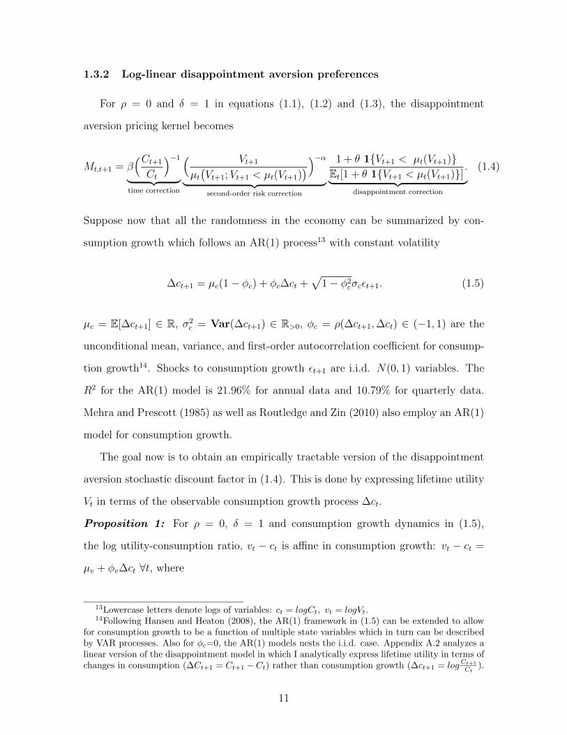
1.3.2 Log-linear disappointment aversion preferences

For ρ = 0 and δ = 1 in equations (1.1), (1.2) and (1.3), the disappointment

aversion pricing kernel becomes

Mt,t+1 = β(Ct+1

Ct

)−1

︸ ︷︷ ︸time correction

( Vt+1

µt(Vt+1;Vt+1 < µt(Vt+1)

))−α︸ ︷︷ ︸second-order risk correction

1 + θ 1{Vt+1 < µt(Vt+1)}Et[1 + θ 1{Vt+1 < µt(Vt+1)}]

.︸ ︷︷ ︸disappointment correction

(1.4)

Suppose now that all the randomness in the economy can be summarized by con-

sumption growth which follows an AR(1) process13 with constant volatility

∆ct+1 = µc(1− φc) + φc∆ct +√

1− φ2cσcεt+1. (1.5)

µc = E[∆ct+1] ∈ R, σ2c = Var(∆ct+1) ∈ R>0, φc = ρ(∆ct+1,∆ct) ∈ (−1, 1) are the

unconditional mean, variance, and first-order autocorrelation coefficient for consump-

tion growth14. Shocks to consumption growth εt+1 are i.i.d. N(0, 1) variables. The

R2 for the AR(1) model is 21.96% for annual data and 10.79% for quarterly data.

Mehra and Prescott (1985) as well as Routledge and Zin (2010) also employ an AR(1)

model for consumption growth.

The goal now is to obtain an empirically tractable version of the disappointment

aversion stochastic discount factor in (1.4). This is done by expressing lifetime utility

Vt in terms of the observable consumption growth process ∆ct.

Proposition 1: For ρ = 0, δ = 1 and consumption growth dynamics in (1.5),

the log utility-consumption ratio, vt − ct is affine in consumption growth: vt − ct =

µv + φv∆ct ∀t, where

13Lowercase letters denote logs of variables: ct = logCt, vt = logVt.14Following Hansen and Heaton (2008), the AR(1) framework in (1.5) can be extended to allow

for consumption growth to be a function of multiple state variables which in turn can be describedby VAR processes. Also for φc=0, the AR(1) models nests the i.i.d. case. Appendix A.2 analyzes alinear version of the disappointment model in which I analytically express lifetime utility in terms ofchanges in consumption (∆Ct+1 = Ct+1 −Ct) rather than consumption growth (∆ct+1 = logCt+1

Ct).

11

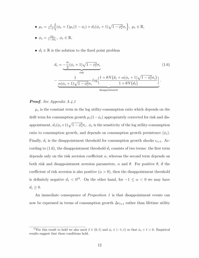
• µv = β1−β

{(φv + 1)µc(1− φc) + d1(φv + 1)

√1− φ2

cσc

}, µv ∈ R,

• φv = βφc1−βφc , φv ∈ R,

• d1 ∈ R is the solution to the fixed point problem

d1 = −α2

(φv + 1)√

1− φ2cσc︸ ︷︷ ︸

risk

(1.6)

− 1

α(φv + 1)√

1− φ2cσc

log[1 + θN

(d1 + α(φv + 1)

√1− φ2

cσc)

1 + θN(d1

) ]︸ ︷︷ ︸

disappointment

.

Proof. See Appendix A.4.1

µv is the constant term in the log utility-consumption ratio which depends on the

drift term for consumption growth µc(1−φc) appropriately corrected for risk and dis-

appointment, d1(φv+1)√

1− φ2cσc. φv is the sensitivity of the log utility-consumption

ratio to consumption growth, and depends on consumption growth persistence (φc).

Finally, d1 is the disappointment threshold for consumption growth shocks εt+1. Ac-

cording to (1.6), the disappointment threshold d1 consists of two terms: the first term

depends only on the risk aversion coefficient α, whereas the second term depends on

both risk and disappointment aversion parameters, α and θ. For positive θ, if the

coefficient of risk aversion is also positive (α > 0), then the disappointment threshold

is definitely negative d1 < 015. On the other hand, for −1 ≤ α < 0 we may have

d1 ≥ 0.

An immediate consequence of Proposition 1 is that disappointment events can

now be expressed in terms of consumption growth ∆ct+1 rather than lifetime utility

15For this result to hold we also need β ∈ (0, 1) and φc ∈ (−1, 1) so that φv + 1 > 0. Empiricalresults suggest that these conditions hold.

12

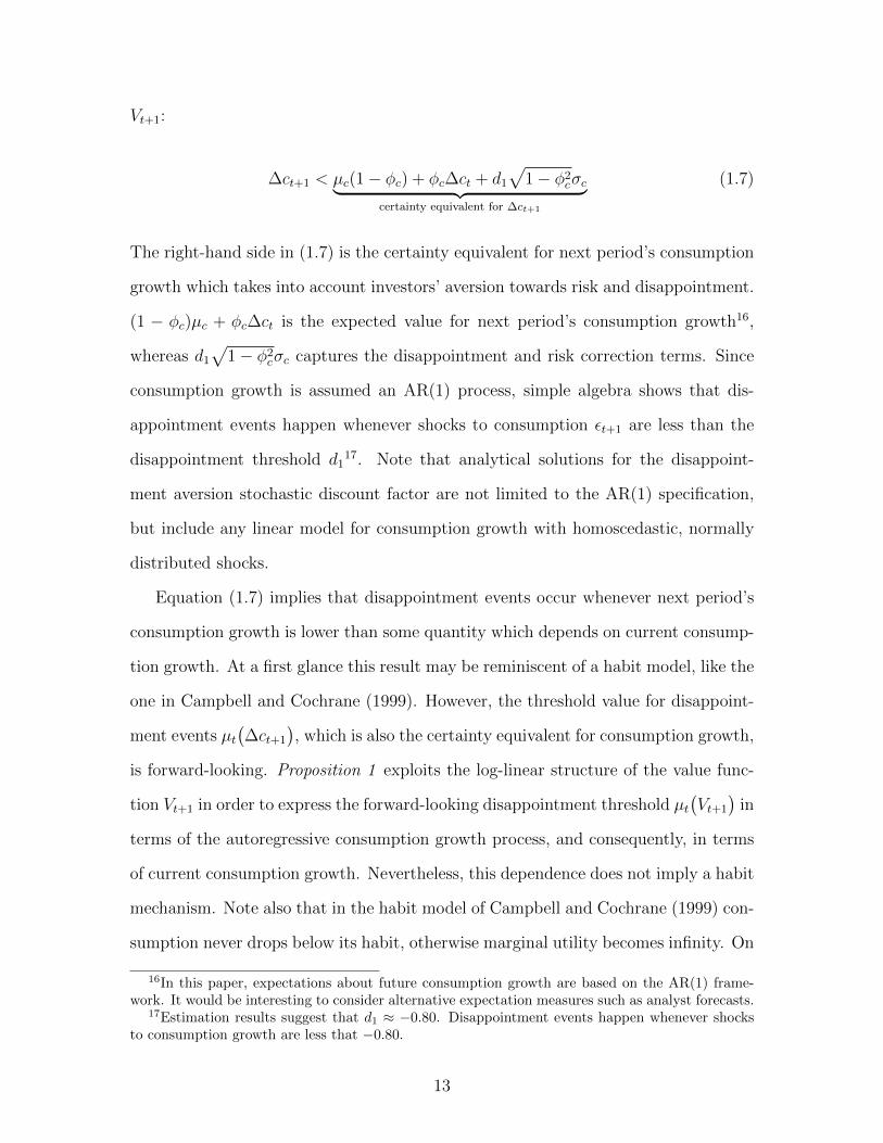
Vt+1:

∆ct+1 < µc(1− φc) + φc∆ct + d1

√1− φ2

cσc︸ ︷︷ ︸certainty equivalent for ∆ct+1

(1.7)

The right-hand side in (1.7) is the certainty equivalent for next period’s consumption

growth which takes into account investors’ aversion towards risk and disappointment.

(1 − φc)µc + φc∆ct is the expected value for next period’s consumption growth16,

whereas d1

√1− φ2

cσc captures the disappointment and risk correction terms. Since

consumption growth is assumed an AR(1) process, simple algebra shows that dis-

appointment events happen whenever shocks to consumption εt+1 are less than the

disappointment threshold d117. Note that analytical solutions for the disappoint-

ment aversion stochastic discount factor are not limited to the AR(1) specification,

but include any linear model for consumption growth with homoscedastic, normally

distributed shocks.

Equation (1.7) implies that disappointment events occur whenever next period’s

consumption growth is lower than some quantity which depends on current consump-

tion growth. At a first glance this result may be reminiscent of a habit model, like the

one in Campbell and Cochrane (1999). However, the threshold value for disappoint-

ment events µt(∆ct+1

), which is also the certainty equivalent for consumption growth,

is forward-looking. Proposition 1 exploits the log-linear structure of the value func-

tion Vt+1 in order to express the forward-looking disappointment threshold µt(Vt+1

)in

terms of the autoregressive consumption growth process, and consequently, in terms

of current consumption growth. Nevertheless, this dependence does not imply a habit

mechanism. Note also that in the habit model of Campbell and Cochrane (1999) con-

sumption never drops below its habit, otherwise marginal utility becomes infinity. On

16In this paper, expectations about future consumption growth are based on the AR(1) frame-work. It would be interesting to consider alternative expectation measures such as analyst forecasts.

17Estimation results suggest that d1 ≈ −0.80. Disappointment events happen whenever shocksto consumption growth are less that −0.80.

13

the other hand, for disappointment aversion preferences it is precisely periods during

which consumption growth falls below its certainty equivalent that are important for

asset prices.

Using the results in Proposition 1, the disappointment aversion discount factor

becomes

Mt,t+1 = exp[logβ −∆ct+1︸ ︷︷ ︸

time correction

(1.8)

+αµc

1− βφc(1− φc)−

α2σ2c

2(1− βφc)2(1− φ2

c)−α

1− βφc∆ct+1 +

α

βφv∆ct

]︸ ︷︷ ︸

second-order risk correction

×1 + θ1{∆ct+1 < µc(1− φc) + φc∆ct + d1

√1− φ2

cσc}1 + θEt

[1{∆ct+1 < µc(1− φc) + φc∆ct + d1

√1− φ2

cσc + α(φv + 1)(1− φ2c)σ

2c}]︸ ︷︷ ︸

disappointment (first-order risk) correction

,

Mt,t+1 in (1.8) corrects expected future payoffs for timing, risk and disappointment18,

much like the discount factor in (1.4). The crucial difference between the two ex-

pressions is that in equation (1.8) unobservable lifetime utility Vt+1 is expressed in

terms of the observable consumption growth ∆ct+1. The empirically relevant terms

in (1.8) which affect expected excess stock returns are future consumption growth

terms (∆ct+1), and the disappointment aversion indicator function.

The disappointment model yields an analytical solution for the risk-free rate as

18Excluding time-correction terms, exp(logβ−∆ct+1

), the expected value of the remaining terms

in (1.8) should equal one, since the risk and disappointment correction terms induce a new probabilitymeasure on the space of asset returns and consumption growth.

14

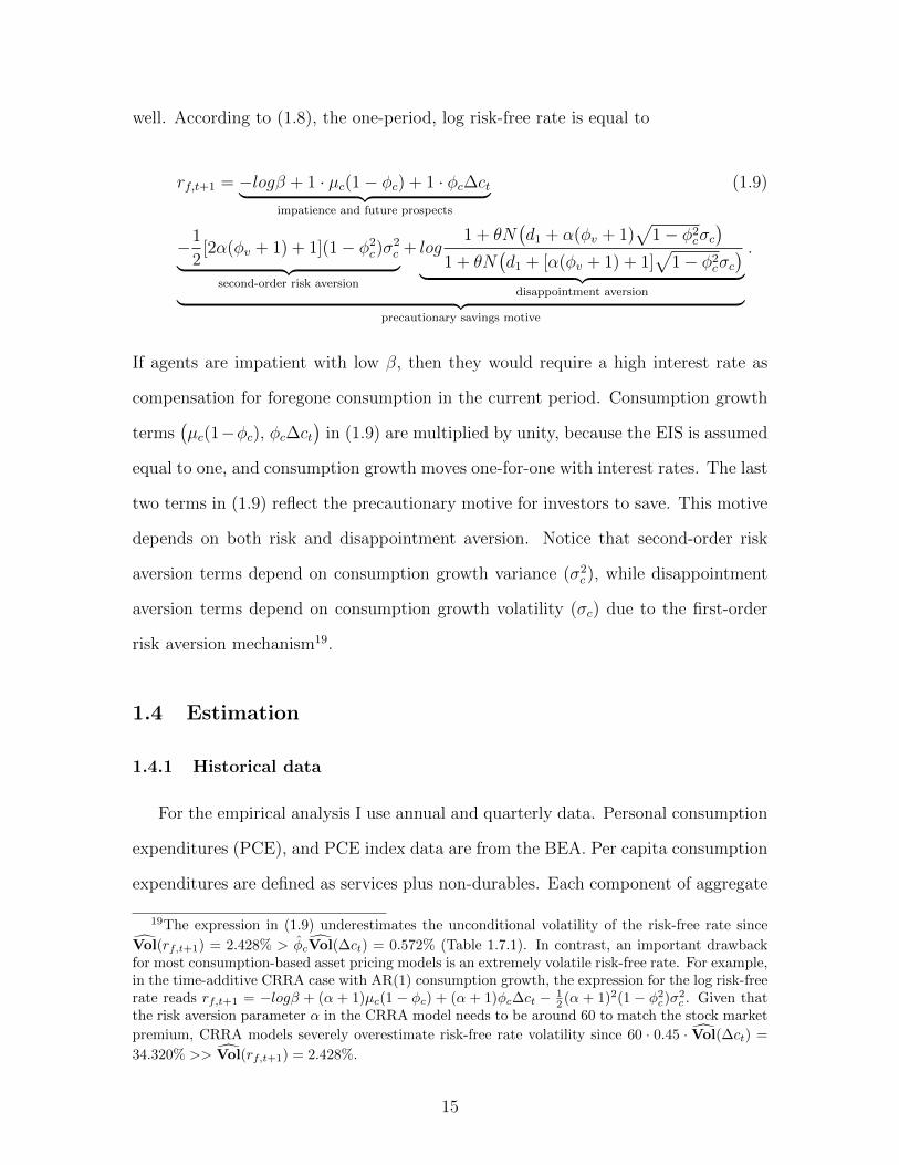
well. According to (1.8), the one-period, log risk-free rate is equal to

rf,t+1 = −logβ + 1 · µc(1− φc) + 1 · φc∆ct︸ ︷︷ ︸impatience and future prospects

(1.9)

−1

2[2α(φv + 1) + 1](1− φ2

c)σ2c︸ ︷︷ ︸

second-order risk aversion

+ log1 + θN

(d1 + α(φv + 1)

√1− φ2

cσc)

1 + θN(d1 + [α(φv + 1) + 1]

√1− φ2

cσc)︸ ︷︷ ︸

disappointment aversion︸ ︷︷ ︸precautionary savings motive

.

If agents are impatient with low β, then they would require a high interest rate as

compensation for foregone consumption in the current period. Consumption growth

terms(µc(1−φc), φc∆ct

)in (1.9) are multiplied by unity, because the EIS is assumed

equal to one, and consumption growth moves one-for-one with interest rates. The last

two terms in (1.9) reflect the precautionary motive for investors to save. This motive

depends on both risk and disappointment aversion. Notice that second-order risk

aversion terms depend on consumption growth variance (σ2c ), while disappointment

aversion terms depend on consumption growth volatility (σc) due to the first-order

risk aversion mechanism19.

1.4 Estimation

1.4.1 Historical data

For the empirical analysis I use annual and quarterly data. Personal consumption

expenditures (PCE), and PCE index data are from the BEA. Per capita consumption

expenditures are defined as services plus non-durables. Each component of aggregate

19The expression in (1.9) underestimates the unconditional volatility of the risk-free rate since

Vol(rf,t+1) = 2.428% > φcVol(∆ct) = 0.572% (Table 1.7.1). In contrast, an important drawbackfor most consumption-based asset pricing models is an extremely volatile risk-free rate. For example,in the time-additive CRRA case with AR(1) consumption growth, the expression for the log risk-freerate reads rf,t+1 = −logβ + (α + 1)µc(1 − φc) + (α + 1)φc∆ct − 1

2 (α + 1)2(1 − φ2c)σ

2c . Given that

the risk aversion parameter α in the CRRA model needs to be around 60 to match the stock market

premium, CRRA models severely overestimate risk-free rate volatility since 60 · 0.45 · Vol(∆ct) =

34.320% >> Vol(rf,t+1) = 2.428%.

15

consumption expenditures is deflated by its corresponding PCE price index (base

year is 2004). Population data are from the U.S. Census Bureau. Recession dates are

from the NBER. Asset returns, factor returns, and interest rates are from Kenneth

French’s (whom I kindly thank) website. Stock returns and interest rates have been

adjusted for inflation by subtracting the growth rate of the PCE price index20. For

quarterly data, I follow the “beginning-of-period” convention as in Campbell (2003)

and Yogo (2006) because beginning-of-quarter consumption growth is better aligned

with stock returns.

Annual consumption data are from 12/31/1948 to 12/31/2011, whereas quarterly

consumption data are from 1948.Q1 to 2011.Q4. Annual asset returns are cum-

dividend, equal-weighted returns from 12/31/1949 to 12/31/2011 with the exception

of earnings-to-price portfolios which start on 12/31/1952. Quarterly returns are from

1948.Q2 up to 2011.Q4. Following Liu et al. (2009), I focus on equal-weighted portfo-

lios which exhibit more pronounced cross-sectional dispersion, and do not overweigh

large firms. Following Yogo (2006), I start the sample in the late 40’s in order to

allow sufficient time for Second World War shocks to die out. The use of post-war

data is motivated by the possibility of a structural break in the U.S. economy af-

ter the Second World War, as well as by the fact that consumption and population

measurements during the first half of the 20th century may not be accurate21.

1.4.2 Estimation methodology

My analysis is focused on portfolios double sorted on size and book-to-market

(BM). Ever since Fama and French (1993 & 1996) documented that these two vari-

ables capture most of the cross-sectional variation in equity returns, much of the

20Rreal,t+1 = exp(logRnom,t+1 − log PCEt+1

PCEt), R are gross returns.

21This study focuses on 25 portfolios double sorted on book-to-market and size. Estimationresults for 10 BM portfolios, 10 size portfolios, 10 BM and 10 size portfolios combined, value-weighted portfolios, nominal consumption growth and nominal stock returns, as well as results forthe 1930-2011 period are available upon request.

16

asset pricing literature in the past two decades has focused on explaining the size

and value factors. Parameters to be estimated are the rate of time preference β, the

second-order risk aversion parameter α, and the disappointment aversion parame-

ter θ. The key insight for disappointment aversion preferences is that the reference

point for disappointment d1 is endogenous. According to equation (1.6), d1 will be

identified once preference parameters and consumption growth moments have been

estimated. Consumption growth moments (mean µc, autocorrelation φc, volatility σc)

are estimated in advance, and are considered inputs for the GMM estimation22.

Estimation is conducted using the generalized method of moments (GMM, Hansen

and Singleton 1982) in which the unconditional consumption-Euler equations serve

as moment restrictions

g(β, α, θ) =

E[Mt,t+1

(Ri,t+1 −Rf,t+1

)]for i = 1, 2, ..., n− 1

E[

Mt,t+1

1+θEt[1{∆ct+1<φc∆ct+µc(1−φc)+d1

√1−φ2

cσc+α(φv+1)(1−φ2c)σ

2c}]Rf,t+1

]− 1

, (1.10)

with

Mt,t+1 = exp[logβ + α(φv + 1)µc(1− φc)−

α2

2(φv + 1)2(1− φ2

c)σ2c (1.11)

−[α

1− βφc+ 1]∆ct+1 +

α

βφv∆ct

](1 + θ1{∆ct < µc(1− φc) + φc∆ct+1 + d1

√1− φ2

cσc}),

Ri,t are one-period, real, cum-dividend, gross returns for portfolio i, and Rf,t is the one

period risk-free rate. It is important to emphasize that, contrary to the majority of

cross-sectional results in the literature, moment conditions include the Euler equation

for the risk-free rate in order to examine whether the disappointment model can

explain the cross-section of expected stock returns while generating realistic first and

22In untabulated results, I also consider the case where consumption moments are part of theGMM objective function, and results still go through.

17

second moments for the risk-free rate23.

We can also use the unconditional consumption-Euler equations in (1.10), and the

definition of covariances24 to obtain an explicit formula for model-implied expected

returns

ˆE[Ri,t+1] = E[Rf,t+1]− 1

E[Mt,t+1]Cov[Ri,t+1 −Rf,t+1, Mt,t+1], (1.12)

m.a.p.e. =1

n

n∑i=1

∣∣ ˆE[Ri,t+1]− E[Ri,t+1]∣∣.

Mt,t+1 is from (1.11),ˆE[Ri,t] are model-implied expected returns, and E[Ri,t] are

sample expected returns. Mean absolute prediction error (m.a.p.e.) is a metric which

shows how well the model fits expected returns.

Parameters are estimated by minimizing the sample analogue of the GMM objec-

tive function (g(β, α, θ)) with respect to the unknown preference parameters

min{β, α, θ}

g(β, α, θ)′ W g(β, α, θ). (1.13)

Moment conditions are weighted by the identity matrix (first-stage GMM). According

to Cochrane (2001) and Liu et al. (2009), first-stage GMM preserves the economic

structure of the GMM objective function. Furthermore, according to Ferson and

Foerster (1994), second-stage GMM estimates are distorted in finite samples. Hayashi

(2000, p. 229) and references therein also provide a discussion on small sample GMM

estimators, and suggest the use of first-stage GMM in finite samples. Although first-

stage GMM estimates are consistent (Cochrane 2001, p. 203), standard errors need

to be adjusted for the fact that first-stage GMM does not use the minimum variance

weighting matrix (Cochrane 2001, p. 205).

23The risk-free rate is assumed conditionally risk-free. Unconditionally, the risk-free rate becomesa random variable.

24Cov(X,Y ) = E[XY ]− E[X]E[Y ].

18

Estimation of the disappointment model is challenging because the discount factor

in (1.8) is not continuous. However, Newey and McFadden (1994) and Andrews

(1994) have shown that continuity and differentiability of the GMM objective function

can be replaced by the less stringent conditions of continuity with probability one

(Theorem 2.6 p. 2132 in Newey and McFadden 1994) and stochastic differentiability

(Theorems 7.2 p. 2186, and 7.3 p. 2188, in Newey and McFadden 1994). As shown in

Appendix A.3, both of these conditions are satisfied by the disappointment aversion

stochastic discount factor provided that log-consumption growth and log-stock returns

are continuous random variables (no mass points) with bounded first and second

moments, and a well defined moment generating function. In this case, discontinuities

are zero probability events.

For comparison purposes, I estimate five additional models: the market discount

factor (Lintner 1965), the four factor Fama-French-Carhart (FF) model (Fama and

French 1996, Carhart 1997) model, the time-additive CRRA discount factor defined

over consumption (Mehra and Prescott 1985)

M(CRRA)t,t+1 = βe−(α+1)∆ct+1 , (1.14)

the Epstein-Zin (EZ) pricing kernel with AR(1) consumption growth and log-time

aggregator (Epstein and Zin 1989, Hansen and Heaton 2008)25

M(EZ)t,t+1 = (1.15)

exp[log(β) +

αµc1− βφc

(1− φc)−α2σ2

c

2(1− βφc)2(1− φ2

c)−α

1− βφc+ 1]∆ct+1 +

α

βφv∆ct

],

25The EIS in Epstein-Zin preferences is not necessarily one as it is assumed here. However,throughout the paper I will refer to the non-separable model with second-order risk aversion andlog-time preferences as the Epstein-Zin model. The discount factor in (1.15) is derived along thelines of Proposition 1 with the additional assumption that the coefficient of disappointment aversionθ is zero (no first-order risk aversion effects).

19

and finally, a linear version of the disappointment aversion discount factor2627:

M(LDA)t,t+1 = β

1 + θ 1{∆Ct+1 < µC + d1ΣC}1 + θ Et[1{∆Ct+1 < µC + d1ΣC}]

. (1.16)

The market and Fama-French-Carhart specifications are considered benchmark

models among practitioners and academics. According to Cochrane (2001, p. 442),

the Fama-French-Carhart (FF) model can be regarded as an arbitrage pricing the-

ory model (APT) ”rather than a macroeconomic factor model.” However, due to its

popularity, I include it in the set of asset pricing models. The time-additive CRRA

discount factor in (1.14) requires extremely large values for the second-order risk aver-

sion and rate of time preference parameters in order to match equity returns. The

Epstein-Zin framework does not account for disappointment aversion, yet it relies on

second-order risk aversion and consumption growth persistence in order to generate

realistic equity premia. The linear disappointment model in (1.15) with i.i.d. changes

in consumption highlights the explanatory power of disappointment aversion alone,

without considering second-order risk aversion or persistence in consumption growth.

Consumption models in (1.14) - (1.16) are essentially nested by the benchmark model

in (1.8).

1.4.3 Estimation results for annual stock returns

Table 1.7.2 shows estimation results for the the 25 Fama-French portfolios and

the disappointment aversion discount factor. According to the J-test and p-value

statistics (20.087 and 0.636 respectively), the null hypothesis that all moment condi-

tions are jointly zero cannot be rejected at conventional confidence levels. The rate

26The linear version of the disappointment aversion discount factor is discussed in AppendixA.2, and derived in Appendix A.4.2. µC and ΣC are the unconditional mean and standard devia-tion respectively for consumption in first differences (∆Ct+1) which, in turn, is assumed to be ani.i.d. process with normal shocks. d1 is the disappointment threshold for the linear disappointmentaversion discount factor, and is defined in Appendix A.4.2 (equation A.17).

27An undesirable aspect of the linear disappointment models is the non-zero, but infinitesimallysmall, probability of negative consumption.

20

of time preference β is equal to 0.977 (t-statistic 2.868), whereas the disappointment

aversion coefficient θ is 4.606 (t-statistic 3.883). The estimated value for θ implies

that an extra dollar of consumption during disappointment years is approximately 5.5

times more valuable in terms of marginal utility than an extra dollar of consumption

during normal times. The second-order risk aversion coefficient is 9.929, yet the low

t-statistic (t-stat. 0.574) suggests that α cannot be accurately estimated by GMM.

Kahneman and Tversky (1992) estimate the loss aversion coefficient to be 1.25,

and the second-order risk aversion parameter α to be -0.88. Barberis et al. (2001)

also use a loss aversion parameter of 1.25, yet they set the second-order risk aversion

parameter equal to zero (log-preferences over risk) and prescribe preferences over con-

sumption as well as individual asset returns, whereas here investors have preferences

over consumption alone. In order to explain the market-wide equity premium, Rout-

ledge and Zin (2010) set θ equal to 9 with α equal to -1 (second-order risk neutrality),

whereas in Bonomo et al. (2011) θ is 2.33 and α is 1.5 because the authors assume

a very persistent process for resumption growth variance, whereas here consumption

growth variance is constant.

Choi et al. (2007) conduct clinical experiments on portfolio choice under uncer-

tainty, and find disappointment aversion coefficients that range from 0 to 1.876, with

a mean of 0.39. They also estimate second-order risk aversion parameters that range

from -0.952 to 2.871, with a mean of 1.448. Using experimental data on real effort

provision, Gill and Prowse (2012) estimate disappointment aversion coefficients rang-

ing from 1.260 to 2.070. Ostrovnaya et al. (2006) estimate disappointment aversion

parameters from stock market data using market wide stock market returns as the

explanatory variable, instead of consumption growth. Their estimates for θ range

from 1.825 to 2.783. However, the authors rely on aggregate stock market returns as

an explanatory variable, which are much more volatile than consumption growth.

The main reason as to why parameter estimates may deviate from those obtained

21

in clinical experiments is probably limited stock market participation. It has been

well documented (Mankiw and Zeldes 1991, Jorgensen 2002) that only a fraction of

households participate in the stock market. If aggregate consumption is less volatile

than stock-market participants’ consumption, then parameter estimates using aggre-

gate consumption will be upwards biased.

According to Table 1.7.2, the disappointment threshold d1 is -0.780, which means

that disappointment events happen whenever annual consumption growth is less than

1.031% + 0.463∆ct− 0.780 · 1.120%. These events happen with a 15.873% probability

in the post-war sample28. This is in sharp contrast to the disaster literature (Barro

2006) which indicates that disasters happen with probability 1.7% per year, and to

the results in Ostrovnaya et al. (2006) which identify only 4 disappointment months

for a period from 1960 to 2005. Barro (2006) calibrates the disaster process, an ad-

ditional risk process, to OECD log-output data, whereas here disappointment events

arise endogenously from investor preferences over consumption. In Ostrovnaya et al.

(2006), disappointment events happen rarely because reference levels for disappoint-

ment, in terms of the generalized disappointment aversion coefficient δ, are low. In

their model, the aggregate investor penalizes extreme events since δ < 1, whereas

here δ is 1.

Table 1.7.2 also shows GMM estimation results for the extended set of discount

factors. The constant term in the market model is positive (4.377), whereas the

coefficient on the market factor is negative (-3.132). Both parameters are statistically

significant (t-statistics 3.661 and -2.991 respectively), yet the null hypothesis that all

moment conditions are jointly satisfied can be rejected (p-value 0.009). Statistically

significant estimates for the Fama-French-Carhart model include the constant term

(3.659, t-stat. 2.627), the market parameter (-2.268, t-stat. 1.931), and the HML

coefficient (-3.956, t-stat. -3.058). The null hypothesis for the Fama-French-Carhart

28Disappointment years for the log-linear disappointment aversion discount factor happened in1953, 1956, 1959, 1973, 1980, 1990, 1999, 2007, 2008, 2010.

22

model is also rejected (p-value 0.023). According to Hayashi (2000, p. 229), the low

J-statistics across all asset pricing models in Table 1.7.2 can be attributed to the fact

that first-stage GMM tests of overidentifying restrictions tend to reject the null more

often than they should.

Results for time-separable preferences (CRRA model) reaffirm the equity premium

puzzle in Mehra and Prescott (1985) since the second-order risk aversion parameter

is extremely high (55.17129, t-stat. 2.561). With time-separable CRRA preferences, a

large coefficient of risk aversion is the only way to map consumption growth risk into

equity premia. Moreover, the rate of time preference β is significantly larger than one

(2.17230, t-stat. 3.334) so that the unconditional mean for the risk-free rate remains

low despite the large risk aversion coefficient. Nevertheless, a risk aversion parameter

equal to 55 implies an extremely volatile risk-free rate. Finally, the null hypothesis

for this model is rejected at conventional confidence levels (p-value 0.002).

Contrary to the CRRA case, the estimated rate of time preference for the Epstein-

Zin model is lower than one (0.983, t-stat. 9.395). Also, the second-order risk aversion

parameter (35.55031, t-stat. 3.336) is smaller than for CRRA utility because, with

Epstein-Zin preferences, consumption growth risk is amplified by consumption growth

persistence. However, in untabulated results for i.i.d., instead of AR(1), consumption

growth, the risk aversion estimate for Epstein-Zin preferences is 55.171 (t-stat. 2.537),

exactly identical to the time-additive CRRA case.

The Epstein-Zin discount factor can explain the cross-section of returns with low

values for the second-order risk aversion parameter α provided that consumption

growth is extremely persistent. A number of recent asset pricing results rely on highly

persistent shocks to expected consumption growth. In Bansal and Yaron (2004),

29Cochrane (2001) argues that time-additive CRRA preferences can explain the unconditionalequity premium provided that the risk aversion parameter is larger than 50.

30Liu et al. (2009) and Yogo (2004) also estimate β larger than one for time-additive CRRApreferences.

31In Routldege and Zin (2010), the risk aversion parameter α for the Epstein-Zin model is cali-brated to 31.542.

23

shocks to expected consumption growth have a half-life of approximately 3 years32,

whereas, according to BEA data from Table 1.7.1, shocks to consumption growth

have a half-life of less than a year. Of course, consumption growth persistence and

expected consumption growth persistence are two different quantities. Nevertheless,

the persistent shocks in expected consumption growth assumed by the Bansal-Yaron

model are hard to detect empirically (Beeler and Campbell 2012). Furthermore,

a number of authors (Campbell and Cochrane 1999, Cochrane 2001) suggest that

consumption growth is most likely an i.i.d. process.

When preferences are time-separable, expected excess log-returns are a function

of covariances between stock returns and consumption growth. According to the

expression in (1.14), these covariances are amplified by the second-order risk aversion

coefficient α33:

E[ri,t+1 − rf,t+1]CRRA ≈ (α + 1)Cov(∆ct+1, ri,t+1 − rf,t+1

). (1.17)

When preferences are non-separable (Epstein-Zin model), then expected excess log-

returns are still generated by covariances between stock returns and consumption

growth. However, according to the expression in (1.15), the second-order risk aversion

coefficient α, which amplifies covariances, is divided by 1−βφc, the term that captures

consumption growth persistence

E[ri,t+1 − rf,t+1]EZ ≈ (α

1− βφc+ 1)Cov

(∆ct+1, ri,t+1 − rf,t+1

). (1.18)

If consumption growth persistence φc or the rate of time preferences β are high

enough so that 1 − βφc ≈ 0, then covariances of consumption growth with stock

returns can generate plausible equity risk premia, even if the coefficient of risk aversion

32The half-life of consumption growth shocks when consumption growth follows an AR(1) processis equal to log(0.5)/log(φAR(1)) in which φAR(1) is the first-order autocorrelation coefficient.

33ri,t = logRi,t

24

α is low. For φc = 0 however, risk aversion estimates for the Epstein-Zin model

are the same as in the time-separable case. If additionally we allow the elasticity

of intertemporal substitution to be greater than one, instead of unitary EIS as is

assumed here, then the effects of consumption growth persistence will be even more

pronounced. Beeler and Campbell (2012) highlight the interaction between expected

consumption growth persistence and an EIS higher than one as the main driving force

behind equity risk premia in the long-run risk model of Bansal and Yaron (2004). In

the long-run risk model, equity premia are almost zero if the EIS is lower than one

or if consumption growth is i.i.d.34, unless one assumes extremely high values for the

coefficient of risk aversion α.

Turning to the linear disappointment model in (1.16), the disappointment thresh-

old d1 is -0.913, higher than the threshold for the log-linear case (-0.780 in Table

1.7.2). Similarly, disappointment events for the linear model happen with probabil-

ity 11.111%, and are less frequent relative to the log-linear case35. The rate of time

preference for the linear disappointment aversion model is 0.987 (t-stat. 340.996)36,

and the disappointment aversion coefficient θ is 9.33137 (t-stat. 1.070). The GMM

cannot accurately estimate the disappointment aversion for the linear model probably

because the GMM function remains constant for a range of θ values. Nevertheless,

with a p-value of 0.074 the null hypothesis for the linear disappointment model cannot

be rejected at a 5% confidence level.

Table 1.7.2 also shows mean absolute prediction errors (m.a.p.e.) across all models,

and Figure 1.8.1 shows fitted and sample expected returns according to the expression

in (1.12). Prediction errors for the disappointment aversion discount factors (log-

34Table 4, p. 23 in Bonomo et al. (2011).35Disappointment years for the linear disappointment aversion discount factor happened in 1957,

1973, 1979, 1980, 1990, 2007, 2008.36The high t-statistic is due to the fact that the linear disappointment model exactly pins down

the rate of time preference β from the moment condition E[Rf,t+1β] = 1.37For their version of the linear model, Routledge and Zin (2010) set the disappointment aversion

parameter equal to 9.

25

linear m.a.p.e. 0.99%, linear m.a.p.e. 0.99%) are smaller than for the rest of the

models. The market model is the least accurate model since average prediction error is

2.38% and fitted returns in Figure 1.8.1 (graph b) are almost parallel to the horizontal

axis. The Fama-French-Carhart model does a better job than the market model (FF

m.a.p.e. 1.12%), and its accuracy is superior to consumption models (CRRA m.a.p.e.

1.51%, EZ m.a.p.e. 1.35%). However, in-sample prediction errors for the Fama-

French-Carhart specification are slightly lager than the errors for the disappointment

aversion models. In accordance to m.a.p.e. results, fitted expected returns for the

disappointment models (plots a & f in Figure 1.8.1) are aligned in an orderly fashion

along the 45◦ line.

Relative to the time-additive CRRA and Epstein-Zin models in (1.14) and (1.15),

the log-linear disappointment aversion discount factor in (1.8) has an additional free

parameter, the disappointment aversion coefficient θ. We would therefore expect

the disappointment aversion discount factor to fit the data better than traditional

consumption models. However, results in Table 1.7.2 and Figure 1.8.1 suggest that the

linear disappointment discount factor performs better than the CRRA and Epstein-

Zin discount factors while maintaining the same number of free parameters.

The empirical performance of disappointment aversion preferences can be ex-

plained by three important characteristics. The first one is common to all consump-

tion models, and is related to consumption smoothing. During bad times, when

consumption growth is low, the discount factor is high. According to equation (1.12),

assets that covary positively with the stochastic discount factor Mt,t+1, that is as-

sets that perform well in states of the world for which consumption growth is low,

essentially provide insurance to investors. These assets command low, even negative,

expected returns. On the other hand, assets which do well when consumption growth

is high, but perform poorly when consumption growth is low (negative covariance

with the stochastic discount factor), command high expected returns so as to entice

26

the aggregate investor to include these assets in her portfolio.

Second, disappointment averse investors are reluctant to take small bets due to

non differentiable preferences with asymmetric marginal utility over gains and losses.

Aggregate consumption growth exhibits extremely low time-series variability, which in

turn implies very low covariances between assets returns and consumption growth38.

If investors’ preferences are described by continuously differentiable functions, then

these functions need to be extremely concave in order to generate the observed equity

premia. In contrast, with disappointment aversion preferences, whenever disappoint-

ment events occur, there is an upwards jump in marginal utility. Even though these

jumps in marginal utility are smoothed out by the expectation operator, first-order

risk aversion terms amplify shocks to consumption growth, and generate realistic risk

premia with preference parameters which are smaller in magnitude than those in

second-order risk aversion models.

The third characteristic is related to the reference point for disappointment events.

According to the expression in (1.7), reference levels for disappointment and gains are

endogenously defined, and depend on preference parameters α and θ. Furthermore, in

a dynamic setting the expectation-based reference point for disappointment aversion

preferences is forward-looking which matches perfectly the forward-looking nature

of asset prices. On the other hand, most first-order risk aversion models assume

reference points which are exogenously specified. Relative to other first-order risk

aversion models, the disappointment framework seems to provide a more accurate

description of what investors consider gains and losses.

The sceptical reader might argue that by introducing a non-differentiable utility

function, one can reduce the required magnitude of the risk aversion coefficient be-

cause second-order risk aversion and disappointment aversion are perfect substitutes.

While this might be partially true, the discussion in the introductory and literature

38Table 1.7.1.

27

review parts of this paper, and references therein, emphasize important theoretical

differences between the two concepts. First-order risk aversion can resolve a num-

ber of stylized facts about decisions under uncertainty which cannot be explained by

smooth utility functions. If second-order risk aversion and disappointment aversion

were perfect substitutes, then prediction errors in Table 1.7.2 for the two types of

consumption models should be identical. Moreover, expected returns for traditional

consumption models (graphs d and e in Figure 1.8.1) should perfectly match those

for disappointment aversion preferences (graphs a and f).

1.4.4 Disappointment events and NBER recessions

Figure 1.8.2 plots consumption growth, disappointment years, and NBER reces-

sion dates. Disappointment events are estimated from the Euler equations for the

25 Fama-French portfolios plus the risk-free rate, and are highlighted with ellipses.

When consumption growth is i.i.d, the disappointment threshold is constant across

time (the flat line in Figure 1.8.2) and equal to 0.84%39. When consumption growth is

AR(1), the disappointment threshold is time-varying (the dashed line in Figure 1.8.2).

Overall, disappointment events are connected to real economic activity. The stock

market crisis of 1987 or the LTCM bailout in 1998 are not considered disappointment

events since the financial meltdowns did not spill over to aggregate consumption.

Disappointment events emphasize an important aspect of consumption asset pricing

models: financial assets are priced according to the co-movement of these assets with

aggregate consumption and the real economy. Financial crises are therefore priced

into asset returns only to the extent that these crises spill over to the real sector.

This is exactly what happened during the recent 2007-2009 recession.

39For i.i.d. consumption growth, disappointment events are characterized by the threshold µc +d1σc ≈ 0.84%. µc is the unconditional expected consumption growth (1.922% from Table 1.7.1), σcis the unconditional standard deviation for consumption growth (1.264% from Table 1.7.1), and d1

is the disappointment threshold (-0.854 in untabulated results for i.i.d. consumption growth and theset of the 25 Fama-French portfolios plus the risk-free rate).

28

According to Figure 1.8.2, disappointment events tend to pre-date NBER recession

years. In order to test how often disappointment events are followed by recessions,

I run logistic regressions in which the dependent variable is an indicator function

depending on whether there are at least three NBER recession months in year t

Y = 1{at least three months in year t are NBER recession months}.

The explanatory variable is also an indicator function depending on whether year

t− 1 was a disappointment year

X = 1{year t− 1 was a disappointment year}.

Disappointment years are estimated for the set of 25 BM-size portfolios and the

disappointment discount factor in (1.8) with AR(1) consumption growth (the ellipses

in Figure 1.8.2). Panel A in Table 1.7.3 presents results for the logistic regression. If

year t− 1 is a disappointment year, then the probability that there will be more than

three NBER recession months during year t increases from (1 + e1.727)−1 = 15.09%40

to (1 + e1.727−3.806)−1 = 88.88%. Furthermore, since the p-value for the log-likelihood

test is almost zero, we can reject the null hypothesis that the two logistic regression

models, with and without disappointment events as an explanatory variable, have the

same overall fit.

In order to emphasize the fact that disappointment events precede NBER reces-

sions, I repeat the above exercise, but now the explanatory variable is an indicator

function depending on whether year t is also a disappointment year.

X = 1{year t is also a disappointment year}.

4015.09% is the probability that at least three months in year t are NBER recession months giventhat year t− 1 was not a disappointment year.

29

Results in Panel B suggest that disappointment events do not overlap with NBER

recessions since regression coefficients are statistically insignificant (0.251, t-stat.

0.330). Moreover, the high p-value (0.743) indicates that including contemporaneous

disappointment events to the logistic model does not improve the overall fit relative

to the model with the constant term alone. The above results establish that the

set of disappointment events is different than the set of NBER recessions, and that

disappointment events tend to pre-date NBER recessions.

1.4.5 Out-of-sample performance

Consumption-based stochastic discount factors are usually structural models that

rely on deep economic parameters such as the rate of time preference, first or second-

order risk aversion parameters, the elasticity of intertemporal substitution, the elas-

ticity of substitution across different consumption goods, the Frisch elasticity of labor

supply and so on. Estimates for these parameters should remain roughly the same

across time41 and across assets. In this section, the set of asset pricing models is sub-

mitted to a series of out-of-sample performance tests. Besides providing additional

information for the disappointment model, out-of-sample tests can also help address

the critique in Lewellen et al. (2010) on the structural nature of book-to-market

portfolios.

Using estimation results for the 25 Fama-French portfolios in Table 1.7.2, I calcu-

late prediction errors according to the expression in (1.12) when the estimated asset

pricing models are applied to 10 equal-weighted earnings-to-price (EP) portfolios.

Earnings-to-price portfolios have also been used by Fama and French (1993) as test-

ing assets. The stock market portfolio is also included as an out-of-sample testing

asset for consumption models only, since the Fama-French and market models already

include market returns as an asset pricing factor. For the market portfolio tests, I

41The possibility of exogenous time variation in preference parameters is generally unappealingto most economists.

30

also set preference parameters in the log-linear disappointment aversion model equal

to the clinical estimates from Choi et al. (2007): the disappointment aversion param-

eter θ is 1.876, and the second-order risk aversion coefficient α is 2.871. Choi et al.

(2007) perform their clinical experiments in an atemporal setting, and do not provide

any guidance on the choice of β which I set equal to 0.99. Finally, for the Choi et

al. (2007) parametrization, I assume an extremely persistent process for consumption

growth in which the autocorrelation coefficient φc is equal to 0.968.

Panel A in Table 1.7.4 shows out-of-sample results for the set of discount factors

considered in this study and the 10 EP portfolios. Disappointment aversion mod-

els seem to outperform all other models in terms of prediction errors (linear m.a.p.e.

0.40%, log-linear m.a.p.e. 0.80%). According to graph a in Figure 1.8.3, predicted and

sample returns for the disappointment aversion model are almost perfectly aligned

across the diagonal. In terms of the market-wide equity premium (Panel B), dis-

appointment models outperform standard consumption models, and can almost per-

fectly replicate stock market expected returns (linear m.a.p.e. 0.24%), even though

preference parameters have been estimated from the set of 25 Fama-French portfo-

lios. Prediction errors for the Choi et al. (2007) model are also very low (0.15%),

but this is mainly due to consumption growth autocorrelation, which is set equal

to 0.968. Fitted expected returns for the Choi et al. (2007) parametrization with

extremely persistent consumption growth prove that, according to the expression in

(1.18), if consumption growth persistence φc or the rate of time preference β are large

enough, clinical estimates for risk and disappointment aversion parameters can fully

rationalize the equity premium.

In addition to cross-sectional out-of-sample tests, I also study the out-of-sample

accuracy of the asset pricing models across the time-series dimension. First, I esti-

mate model parameters for the extended set of discount factors using stock returns

from 1949 to 1978. Then, I use the estimated parameters to generate model-implied

31

expected returns according to (1.12) for the second half of the sample. For these tests,

I set consumption growth moments (autocorrelation, mean, standard deviation) equal

to the full sample estimates from Table 1.7.1.

Table 1.7.5 shows GMM results for the 1949-1978 sample. Parameter estimates

for the market and Fama-French-Carhart specifications are statistically significant,

and are comparable to the full-sample results from Table 1.7.2, with the exception of

the momentum coefficient (-6.607 vs. 0.268 for the full sample in Table 1.7.2). The

risk aversion estimate for the CRRA model during the 1949-1978 period is 61.229

(t-stat. 2.179), slightly larger than for the full sample. The rate of time preference

for the Epstein-Zin model is higher than one (1.104, t-stat. 5.508), and the second-

order risk aversion estimate is 30.014 (t-stat. 2.706), which is lower than the one

obtained for the full sample in Table 1.7.2. Finally, estimates for the disappointment

aversion parameter θ in the log-linear and linear disappointment models are 3.990

(t-stat. 2.768) and 6.810 (t-stat. 1.980) respectively. None of the models is rejected

since all p-values are large. Nevertheless, standard errors are not reliable, and test

statistics should be interpreted with caution since there are only 30 observations in

the sample.

Table 1.7.5 also shows out-of-sample mean absolute prediction errors for the four

models during the 1979-2011 period. The Fama-French-Carhart model cannot price

expected returns out of sample since the mean absolute prediction error for 1979-2011

period is 13.59%. The market, CRRA, and linear disappointment aversion models do

not do well either, since average out-of-sample errors are equal to 4.10%, 3.22%, and

2.67% respectively. In contrast, the log-linear disappointment aversion and Epstein-

Zin models outperform all other specifications with average prediction errors of 2.17%

and 1.99% respectively. Figure 1.8.4 and Figure 1.8.5 show expected stock returns

for the first and second half of the sample. According to Figure 1.8.4, the Fama-

French-Carhart specification clearly performs better than all other specifications in

32

terms of in-sample accuracy. However, plot c in Figure 1.8.5 shows that the Fama-

French-Carhart model cannot explain out-of-sample expected returns.

Figure 1.8.6 and Figure 1.8.7 show expected stock returns for 10 book-to-market

portfolios during the first and second half of the sample respectively. Estimation re-

sults can be found in Table 1.7.6. In terms of point estimates, results in Table 1.7.6

are quite similar to the ones obtained for the 25 portfolios in Table 1.7.2. Figure

1.8.6 highlights the impressive in-sample performance of the Fama-Frech discount

factor (FF in-sample m.a.p.e. 0.21%). However, out-of-sample prediction errors for

the second half are extremely large (FF out-of-sample m.a.p.e. 10.70%). According

to Figure 1.8.6 and Figure 1.8.7, consumption models exhibit more consistent perfor-

mance across samples than the Fama-French model, and this is probably due to the

structural nature of these models.

Large out-of-sample errors for the Fama-French-Carhart model do not imply that

we should automatically dismiss this model, but rather that its unconditional version

fails to capture time variation in risk premia. Following Ferson and Harvey (1991),

and Jagannathan and Wang (1996), there is a large literature on time-varying betas

which seem to improve the performance of factor-based asset pricing models. On

the other hand, the disappointment model delivers out-of-sample performance with

constant preferences parameters, since time-variation in risk aversion, and therefore

in expected risk premia, is hardwired into disappointment aversion terms. The im-

pressive out-of-sample performance for the disappointment model should also be at-

tributed to better consumption measurements towards the end of the sample, and the

realization of particularly important disappointment events in 1990 and 2007-2008.

33

1.4.6 Estimation results for first-order risk aversion preferences with al-

ternative reference points for gains and losses

The empirical evidence in this paper emphasize the importance of endogenous

reference points for gains and losses in explaining the cross-section of expected stock

returns. In this section, I estimate three additional consumption models which are

very similar to the disappointment aversion stochastic discount factor in (1.8). How-

ever, unlike the disappointment aversion framework, reference points for gains and

losses are no longer equal to the certainty equivalent for consumption growth.

The first-order risk aversion discount factor specification to be tested is

Mt,t+1 = exp[logβ −∆ct+1︸ ︷︷ ︸

time correction

+αµc

1− βφc(1− φc)−

1

2

( ασc1− βφc

)2(1− φ2

c)−α

1− βφc∆ct+1 +

α

βφv∆ct

]×︸ ︷︷ ︸

second-order risk correction

1 + θ1{∆ct+1 < d}1 + θEt

[1{∆ct+1 < d+ α(φv + 1)(1− φ2

c)σ2c}] .︸ ︷︷ ︸

first-order risk correction

(1.19)

in which d is the exogenous reference point for gains and losses. It is straightforward

to show that Mt,t+1 in (1.19) is non-negative and that

Et{exp[α(φv + 1)µc(1− φc)− α2

2σ2c (1− φ2

c)(φv + 1)2 − α1−βφc∆ct+1 + α

βφv∆ct

−log(1 + θEt

[∆ct+1 < d+ α(φv + 1)(1− φ2

c)σ2c

])+ log(1 + θ1{∆ct+1 < d})

]}= 1,

provided that i) consumption growth is log-normal, ii) its dynamics are given by the

expression in (1.5), and iii) φv = βφc1−βφc . Note that utility functions corresponding

to the discount factor in (1.19) are hard, or even impossible, to aggregate because

preferences are no longer homothetic.

Disappointment events are defined in equation (1.7) as years during which con-

34

sumption growth drops below its certainty equivalent. Similarly, we can define loss

events as periods during which consumption growth drops below the threshold d. I

consider four different values for d: i) the log risk-free rate rf,t+1, ii) current period’s

consumption growth ∆ct, iii) zero consumption growth, and iv) d is a free parameter

to be estimated. The above parameter values are intuitively appealing, and have been

previously used in the literature42.

Table 1.7.7 shows results for the discount factor in (1.19). When d is equal to the

log risk-free rate, the probability of a loss event is 33.333%, the rate of time preference

is 0.917 (t-stat. 5.143), the second-order risk aversion estimates is quite high (α =

46.784, t-stat. 3.015), and the disappointment aversion parameter is negative (θ = -

0.827, t-stat. -3.073). When d is equal to current consumption growth, the probability

of a loss event is 53.568%, the rate of time preference is larger than one (1.215, t-

stat. 6.590), the second-order risk aversion estimate (54.227, t-stat. 13.369) is almost

equal to the time-separable CRRA case from Table 1.7.2, and the first-order risk

aversion parameter is negative (-0.916, t-stat. -7.794). We can therefore conclude

that whenever the reference point d is equal to either the log risk-free rate or current

consumption growth, then loss events happen so often that: i) they become irrelevant

for asset pricing, ii) the first-order risk aversion parameter is negative, and iii) the

second-order risk aversion parameter is similar in magnitude to the time-additive

CRRA estimates from Table 1.7.2.

Results are more economically sensible when the reference point for consumption

growth is zero (the status quo). This reference point can also be interpreted as the

outcome of a reference mechanism for consumption in levels: Ct+1 < Ct. In this case,

loss events happen rarely with probability 6.349% because the loss threshold is quite

low. The rate of time preference is lower than one (0.919, t-stat. 11.963), the first-

order risk aversion estimate is quite low (1.511, t-stat. 0.428), and the second-order

42Barberis et al. (2001) and Piccioni (2011) use the risk-free rate as a reference point, whereasin Bernatzi and Thaler (1995) the reference point is zero.

35

risk aversion parameter is equal to 19.297 (t-stat. 0.793).

Finally, estimates for the free threshold model are very similar to the benchmark

disappointment aversion model from Table 1.7.2. The rate of time preference is

lower than one (0.903, t-stat. 4.444), while the first and second-order risk aversion

parameters are equal to 4.113 (t-stat. 2.018) and 13.043 (t-stat. 0.875) respectively.

The estimated reference point for consumption growth, ˆd = 0.47%, is greater than

zero but lower than the i.i.d. disappointment reference level of 0.84% in Figure 1.8.2.

Empirical results for the disappointment aversion and free threshold models suggest

that loss events in consumption-based asset pricing models are triggered by positive

thresholds rather than zero or negative consumption growth.

None of the models in Table 1.7.7 is rejected. However, mean absolute prediction

errors across different models indicate that the relatively high p-values for first-order

risk aversion models are mainly driven by large covariance estimates, rather than zero

means for the error terms. Similarly, mean absolute prediction errors for first-order

risk aversion models are larger than those for the disappointment model in Table

1.7.2. For d = rf,t+1 m.a.p.e. is 2.02%, for d = ∆ct m.a.p.e. is 1.84%, for d = 0

m.a.p.e. is 1.54%, and for the free threshold model with ˆd = 0.47% m.a.p.e. is 1.23%.

Figure 1.8.8 shows fitted expected returns for first-order risk aversion models plus

the disappointment aversion discount factor from (1.8). According to Figure 1.8.8,

the free threshold and disappointment aversion discount factors outperform the rest

of the models in terms of fitted expected returns. The above results highlight the

fact that asymmetric marginal utility alone does not improve the performance of

consumption-based asset pricing models. First-order risk aversion preferences must

be combined with an accurate description of investors’ perception of losses in order

to achieve accurate asset pricing moments.

36

1.4.7 Estimation results for quarterly stock returns

Discrete-time models do not provide any guidelines as to how often investors

should evaluate their wealth, and adjust their consumption. If an optimal consump-

tion rebalancing frequency exists, then it will undoubtedly affect the empirical per-

formance of consumption-based asset pricing models. This section studies the per-

formance of asset pricing models at the quarterly frequency in order to shed more

light on the relevant frequency of consumption adjustments by disappointment averse

individuals.

Table 1.7.8 shows GMM results for the 25 Fama-French portfolios and the set of

discount factors. The intercept for the market discount factor is economically and

statistically significant (4.317, t-stat. 4.342), while the loading on market returns (-

3.253, t-stat. -3.392) is similar to the one estimated from annual data. For the Fama-

French-Carhart model, all terms are statistically significant. According to Table 1.7.8,

the equity premium puzzle is more pronounced for quarterly data since second-order

risk aversion parameters for the time-additive CRRA and Epstein-Zin discount factors

are extremely large: 138.538 (t-stat. 3.368) and 147.910 (t-stat. 1.406) respectively43.

Notice also that the rate of time preference β for CRRA utility is higher than one

(1.483, t-stat. 13.030).

Why are second-order risk aversion estimates for the CRRA and Epstein-Zin mod-

els so large? Gabaix and Laibson (2002) propose a continuous-time model in which at

each point in time only a fraction of investors adjust consumption for a period of D

time-units. The authors show that adjustment delays cause covariances of aggregate

consumption with asset returns to be very low. According to Gabaix and Laibson

(2002), second-order risk aversion parameters should be divided by 6D (“6D bias”)

with D being the adjustment period44. If we believe the 6D bias, and investors adjust

43Aıt-Sahalia et al. (2004) and Yogo (2006) obtain even larger estimates for the second-order riskaversion parameter using quarterly data.

44Breeden et al. (1989) suggest dividing the second-order risk aversion estimate by 2 in order to

37

their consumption every 4 quarters, then quarterly estimates for risk aversion parame-

ters should be equal to 138/(6·4) ≈ 5.75 for CRRA preferences, and 148/(6·4) ≈ 6.16

for the Epstein-Zin model. However, Piazzesi (2002) shows that adjustment delays

in consumption are not enough to generate plausible equity premia, and that the

Gabaix-Laibson model has a number of undesirable implications.

Unlike second-order risk aversion models, preference parameters for the disap-

pointment aversion discount factor remain roughly equal to their annual counterparts.

The disappointment aversion coefficient θ in the linear model is 7.932 (t-stat. 1.412),

whereas for the log-linear disappointment aversion model θ is 5.274 (t-stat. 2.861)

and α is 14.376 (t-stat. 0.352). The disappointment threshold d1 is -0.858 for the

linear model, and -0.774 for the log-linear case, while the probabilities of disappoint-

ment events are 15.294% and 16.862% respectively. Disappointment thresholds and

disappointment event probabilities for quarterly data are similar to those obtained

for annual data in Table 1.7.2 because preference parameters for the two samples

are almost identical. The fact that disappointment aversion parameters remain con-

stant across frequencies, while risk aversion triples in magnitude, emphasizes that

first and second-order risk aversion models are not perfect substitutes, and that the

two specifications have both quantitative and qualitative differences.

According to Table 1.7.8, the CRRA model achieves the lowest mean absolute

prediction error (0.40%) among consumption models, probably because the AR(1)

specification in non-separable preferences does not fit quarterly consumption growth

well (Table 1.7.1). The Fama-French-Carhart specification generates the lowest pre-

diction error among all models (0.24%). Figure 1.8.9 shows predicted and sample

expected returns at the quarterly frequency. Although there is a weak alignment pat-

tern between predicted and sample expected returns for the disappointment discount

factors (graphs a & f), the latter models tend to overestimate expected returns for

correct for the summation bias in consumption measures.

38

low book-to-market portfolios (portfolios 1, 6, 11, and 16).

An important issue that emerges from quarterly data is the disappointing per-

formance of the disappointment models. Bernatzi and Thaler (1995) combine loss

aversion with narrow framing45 under the term “myopic loss aversion”. They pro-

vide evidence that stock market equity premia can be explained by a model in which

loss averse investors evaluate portfolio performance and rebalance consumption infre-

quently:

The longer the investor intends to hold the asset, the more attractive the risky asset

will appear, so long the investment is not evaluated frequently. Bernatzi and Thaler

(1995), p. 75.

My results also suggest that the disappointment aversion discount factor performs

much better at low frequencies. Disappointment aversion preferences do not seem

to work well for high frequencies simply because individuals do not adjust their con-

sumption often enough. The fact that disappointment models fail at the quarterly

frequency may also be related to the results in Dillenberger (2004) and Artstein-

Avidan and Dillenberger (2011) where the authors show that disappointment averse

individuals prefer one-shot over gradual resolution of uncertainty. According to these

results, investors prefer to evaluate their portfolios once a year (one-shot resolution

of uncertainty) rather than gradually accumulate information about portfolio perfor-

mance every quarter, and adjust their consumption accordingly.

Aıt-Sahalia et al. (2004) provide an alternative explanation for the failure of con-

sumption models at higher frequencies which is related to consumption measurement.

They claim that consumption pricing models should focus on consumption of luxury

goods because these goods are more responsive to changes in wealth, and constitute

a better measure for stock market participants’ consumption. Yogo (2006) success-

fully explains quarterly expected returns for 25 Fama-French portfolios using durables

45The fact that investors tend to evaluate new risks in isolation instead of pooling new riskstogether with old ones is usually referred to as “narrow framing”.

39

consumption, even though estimated coefficients for second-order risk aversion are ex-

tremely large (around 200). It might well be the case that consumption of nondurables

and services, which is used here, is unresponsive to wealth performance on a quarterly

basis, while other measures of consumption that include luxury or durable goods co-

vary better with equity returns. Note also that this study uses seasonally adjusted

consumption data from the BEA. Ferson and Harvey (1992) show that the implied

smoothing in seasonally adjusted quarterly data will affect the empirical performance

of consumption-based models.

Overall, results for quarterly data raise two very important questions which are

left for future research: i) What determines optimal consumption rebalancing in-

tervals when investors are disappointment averse? ii) Why are quarterly estimates

for disappointment aversion parameters almost equal to annual estimates, whereas

second-order risk aversion coefficients for time-additive and Epstein-Zin preferences

triple in magnitude?

1.5 Related literature

Before concluding the discussion about disappointment aversion preferences, I

will briefly relate the disappointment framework to previous results on first-order risk

aversion, and to the current state of consumption-based asset pricing literature.

1.5.1 First-order risk aversion preferences

Starting with the seminal paper by Kahneman and Tversky (1979), there has been

an abundance of experimental evidence in favor of first-order risk aversion preferences

(Duncan 2010, Pope and Schweitzer 2011). Kahneman and Tversky (1979) were

also among the first to introduce the concept of loss aversion which describes first-

order risk aversion behavior by means of piece-wise utility functions with exogenous

reference points for gains and losses. However, piece-wise utility functions are not

40

the only way to obtain first-order risk aversion preferences. Epstein and Zin (1990)

show that first-order risk aversion behavior also occurs when investors use concave

functions to rescale cumulative distribution functions of random payoffs. These types

of preferences are usually referred to as rank-dependent preferences (Epstein and Zin

1990).

Even though loss aversion is probably the most widely known approach for model-

ing first-order risk aversion preferences, there are a number of important issues which

until recently have been overlooked by the literature. First, loss aversion preferences

may lead to violations of the continuity and transitivity axioms for choices under

uncertainty (Gul 1991). Second, the original loss aversion framework does not pro-

vide theoretical arguments as to what reference points for gains and losses should be

or how these reference points should be dynamically updated. Towards the end of

their paper, Kahneman and Tversky (1979) essentially discuss time-varying reference

points. However, they do not provide further guidelines on how to construct endoge-

nous reference points within the loss aversion framework. Third, contrary to the well

behaved aggregation properties of the disappointment model, Ingersoll (2011) shows

that loss aversion preferences cannot be aggregated under the standard assumptions

of general equilibrium models.

Segal and Spivak (1990), who were among the first to introduce the term first-

order risk aversion, discuss the full insurance problem46 which can be rationalized

by first-order risk aversion preferences, but cannot be explained by smooth utility

functions. Rabin (2000) argues that smooth utility functions imply an approximately

risk-neutral behavior “not just for negligible stakes, but for quite sizeable and eco-

nomically important stakes”47. He also explains why second-order risk aversion pref-

erences have unappealing implications for large scale risks, a result known as the

46The full insurance puzzle is related to the fact that it is never optimal to purchase full insurancewhen insurance policies are not actuarially fairly priced, but in practice people do so (Mossin 1968).

47Rabin (2000), p. 1281.

41

calibration theorem48. First-order risk aversion models are not immune to calibration

theorems. Safra and Segal (2008) extend Rabin’s (2000) critique on expected utility

to non-expected utility models, like the disappointment aversion model, in which they

assume the presence of background risk (Theorem 2, p. 1151 in Safra and Segal 2008

)49.

Recent empirical results indicate that endogenous reference points are a very im-

portant aspect of first-order risk aversion preferences. Choi et al. (2007) identify

disappointment aversion behavior during clinical experiments on portfolio decisions

under uncertainty. Post et al. (2008) suggest that players’ choices in the TV show

“Deal or No Deal” can be explained by reference-based preferences in which reference

points are affected by previous outcomes experienced during the game. Using a ques-

tionnaire experiment with stock prices, Arkes et al. (2008) identify an asymmetric

adaptation process for reference points which is a function of past decision outcomes

(gains vs. losses).

Doran (2010) and Crawford and Meng (2011) find evidence that taxi drivers set

daily income goals (reference points) which are affected by expectations (slow day vs.

a good day), and these goals change during the course of the day (dynamic updating).

Choice-acclimating reference-dependent preferences have also been well documented

in the context of effort provision by Abeler et al. (2011), while Gill and Prowse (2012)

identify disappointment aversion preferences in real effort competition. They argue

that

Disappointment at doing worse than expected can be a powerful emotion. This emotion

may be particularly intense when the disappointed agent exerted effort in competing

for a prize [...] Furthermore, a rational agent who anticipates possible disappointment

48Appendix A.1 also provides a brief discussion about key differences between first and second-order risk aversion preferences.

49Nevertheless, Chapman and Polkovnichenko (2011) show that if this background risk is a dis-crete random variable and investors have rank-dependent preferences, then Safra and Segal’s (2008)critique cannot be applied.

42

will optimize taking into account the expected disappointment arising from her choice.

Gill and Prowse (2012), p. 469.

Finally, Artstein-Avidan and Dillenberger (2011) show that their dynamic disappoint-

ment aversion framework can explain why individuals tend to pay overpriced fees in

order to insure electric appliances.

First-order risk aversion preferences have already been used in prior attempts to

resolve asset pricing puzzles. Epstein and Zin (1990), Bernatzi and Thaler (1995),

Barberis et al. (2001), Andries (2011), Piccioni (2011), Easley and Yang (2012) are

papers which use loss aversion models or some form of asymmetric marginal utility

over gains and losses in order to explain the equity premium puzzle. However, none

of these papers focuses on the importance of reference points for gains and losses.

Epstein and Zin (2001) integrate models of first-order risk aversion into a recursive

intertemporal asset-pricing framework and find that “risk preferences that exhibit

first-order risk aversion accounts for significantly more of the mean and autocorrela-

tion properties of the data than models that exhibit only second-order risk aversion”

(Epstein and Zin 2001, p. 537). Campanale et al. (2010) introduce disappointment

aversion preferences in a production economy to match the unconditional market-wide

equity premium.

Ang et al. (2005) compare loss and disappointment aversion models, and empha-

size the tractability of disappointment aversion preferences relative to loss aversion.

The authors also argue that if expected excess returns are positive, then smooth utility

functions will necessarily generate positive holdings of risky assets, while first-order

risk aversion preferences can admit corner solutions: zero holdings of risky assets in

spite of positive expected excess returns (non-participation effect). In a similar way,

Khanapure (2012) uses disappointment aversion preferences to rationalize the fact

that investors drastically cut their portfolio allocations on stocks after retirement, a

puzzling behavior that cannot be explained by smooth (CRRA) preferences.

43

Finally, the theoretical framework in this paper assumes identical preferences

across individuals which can then be aggregated due to linear homogeneity of dis-

appointment aversion. Nevertheless, Chapman and Polkovnichenko (2009) show that

in models with first-order risk aversion preferences the equity premium and the risk-

free rate are sensitive to preference heterogeneity, an important implication which is

ignored by the representative agent model.

1.5.2 Consumption-based asset pricing

Throughout this paper, I maintain that BEA consumption accurately depicts eco-

nomic conditions. A number of papers have tried to improve on BEA measures of

consumption by focusing on consumption of stock market participants in Mankiw and

Zeldes (1991), luxury goods consumption like in Aıt-Sahalia et al. (2004), consump-

tion of durable goods in Yogo (2006), or even garbage output as in Savov (2011).

An extremely important aspect of consumption measurement is limited stock market

participation. According to Jorgensen (2002), stock market participants are a small

sub-sample of the total population. Using aggregate consumption as a proxy for stock

market participants’ consumption may lead to inconsistent estimates for preference

parameters. The above strand of literature is complimentary to ours. Combining

more accurate measures of consumption with disappointment aversion preferences

will probably resolve a number of stylized facts in financial markets. Furthermore,

improving upon measures of consumption will also decrease the estimated magnitudes

for risk and disappointment aversion parameters.

It has been well documented that consumption models with time-additive CRRA

preferences require implausibly high values for the risk aversion parameter (Mehra

and Prescott 1985) in order to explain expected stock returns. However, Bansal

and Yaron (2004) show that with non-separable preferences and a persistent mean

in consumption growth, consumption risk can explain stock return moments with

44

plausible parameter values. Furthermore, Bansal et al. (2005) use the concept of

long-run risk and are able to explain 60% of the cross-sectional variation in risk

premia for BM, size and momentum portfolios. However, the persistent shocks in

expected consumption growth implied by the long-run risk framework are difficult to

detect empirically. According to the results for the linear disappointment aversion

discount factor in which consumption changes are i.i.d. (Table 1.7.2 and Figure 1.8.1),

disappointment events can explain stock returns even if there are no risks for the long-

run, and changes in consumption are unpredictable. van Binsbergen et al. (2011)

also find that short-term risks may be more important than long-term ones for the

pricing of dividend strips.

Habit models, like the one proposed by Campbell and Cochrane (1999), are

a promising answer to asset pricing puzzles, mainly because they allow for time-

variation in expected returns. Nevertheless, according to Ljungqvist and Uhlig (2009),

these models imply a weird behavior from the social planner’s point of view: gov-

ernment interventions that destroy part of the endowment may lead to an increase

in welfare. Disappointment events should not be confused with Barro’s (2006) rare

disaster framework either. First, contrary to rare disasters, which are not present in

the post-war U.S. economy, disappointment events can be easily identified and hap-

pen relatively often. Second, disappointment events are endogenously characterized

by investor preferences, and are not exogenously specified as an additional source of

uncertainty.

Ju and Miao (2012) address the equity premium puzzle using the concept of

smooth ambiguity aversion introduced by Klibanoff et al. (2005). Ambiguity es-

sentially refers to uncertainty about the“true” probability distribution of stochastic

variables. Klibanoff et al. (2005) propose a smooth concave “utility” function over

the set of possible distributions for stochastic payoffs which implies that investors

overweigh unfavorable prior distributions. Epstein (2010) highlights some unappeal-

45

ing characteristics of the smooth ambiguity aversion model, and proposes the multiple

priors approach by Gilboa and Scmeidler (1989) instead. Although, uncertainty about

“true” probability distributions for macroeconomic variables and asset returns is a

realistic assumption, I abstain from such considerations, and assume a rational ex-

pectations framework with no uncertainty about probability distributions in order to

focus on the performance of disappointment aversion preferences alone.

1.6 Conclusion

According to Kocherlacota (1996), in order to resolve the equity premium puzzle

(at least) one of the following three assumptions needs to be relaxed: i) CRRA pref-

erences, ii) market completeness, iii) transaction costs. Although, I maintain the last

two assumptions, this paper focuses on the first one, and introduces disappointment

aversion preferences in a general equilibrium framework. This paper is the first to

obtain closed-form solutions for the stochastic discount factor in terms of consump-

tion growth when investors are disappointment averse. Analytical solutions, in turn,

allow for a wide range of empirical tests, including comparisons with more traditional

asset pricing models. Unlike exogenous reference levels proposed by the majority of

first-order risk aversion models, my results highlight that endogenous, expectation-

based reference points for gains and losses, as suggested by disappointment aversion

preferences, are important in explaining the cross-section of equity returns.

At the annual frequency, the disappointment aversion discount factor can explain

expected returns for portfolios sorted on book-to-market, size, earnings-to-price, as

well as the aggregate market portfolio. Comparative results also suggest that at the

annual frequency disappointment aversion preferences outperform traditional asset

pricing models in terms of prediction errors, and that disappointment events tend to

predate NBER recessions. Nevertheless, at higher frequencies the performance of the

disappointment model deteriorates, and this is probably related to the myopic loss

46

aversion effect of Bernatzi and Thaler (1995) or due to consumption measurement

issues. Directions for future research include the pricing of fixed income securities

subject to default risk, introducing disappointment aversion preferences in a pro-

duction economy in order to study investment, production and employment during

disappointment years, or even combining disappointment aversion preferences with

better measures for consumption. Finally, this study establishes that small and value

firms covary more with macroeconomic conditions, and consequently, that these firms

are riskier than big and growth firms respectively. However, a very important ques-

tion that remains unanswered by the literature is what are the fundamental firm-level

characteristics which expose small and value firms to aggregate risk.

47

1.7 Tables

Table 1.7.1 Summary statistics

Consumption and the risk-free rate

annually quarterly∆ct+1 ∆Ct+1 rf ,t+1 ∆ct+1 ∆Ct+1 rf ,t+1

E 1.922% $291.432 1.174% 0.484% $73.254 0.295%σ 1.264% $223.447 2.338% 0.502% $77.705 0.644%

ρ(

∆ct+1, .)

1 0.841 0.087 1 0.876 0.057

ρt,t−1 0.463 0.503 0.701 0.328 0.509 0.736R2 AR(1) 21.968% 24.751% 49.261% 10.796% 25.909% 54.172%

Panel B: 25 Fama-French portfolios

Small/ Medium/ Medium/ Big/Value Growth Medium Value Growth

25 BM-Size E[Ri,t+1] 20.766% 8.419% 11.971% 15.770% 8.204%

annual Cov(∆ct+1, Ri,t+1) 0.0017 0.0009 0.0011 0.0013 0.0010

25 BM-Size E[Ri,t+1] 4.667% 2.120% 2.880% 3.678% 2.006%

quarterly Cov(∆ct+1, Ri,t+1) 0.0001 0.0001 0.0001 0.0001 0.0001

Panel C: stock market, HML, SMB, and MOM factors

market HML SMB MOM

annualE[Ri,t+1] 8.930% 5.126% 2.669% 9.374%

Cov(∆ct+1, Ri,t+1) 0.0010 0.0004 0.0002 -0.0000

quarterlyE[Ri,t+1] 1.778% 1.110% 0.504% 2.319%

Cov(∆ct+1, Ri,t+1) 0.0001 0.0000 0.0000 -0.0000

Table 1.7.1 presents summary statistics for the variables used in this study. ∆ct+1 = log(Ct+1/Ct

)in Panel A is real consumption growth, ∆Ct+1 = Ct+1 − Ct is real consumption in first differences,and rf,t+1 = log

(Rf,t+1

)is the real log risk-free rate. E is the sample mean, σ is the sample

standard deviation, and ρ(

∆ct+1, .)

is the sample correlation coefficient with consumption growth.

ρt,t−1 is the autocorrelation coefficient estimate, and R2 AR(1) is the R-square for the AR(1) model.

Panel B shows summary statistics for real, cum-dividend, equity returns Ri,t for the 25 Fama-Frenchportfolios. HML, SMB, MOM in Panel C are the value, size and momentum factors respectively.

Cov are covariance estimates. More details on consumption data and stock returns can be found insubsection 1.4.1.

48

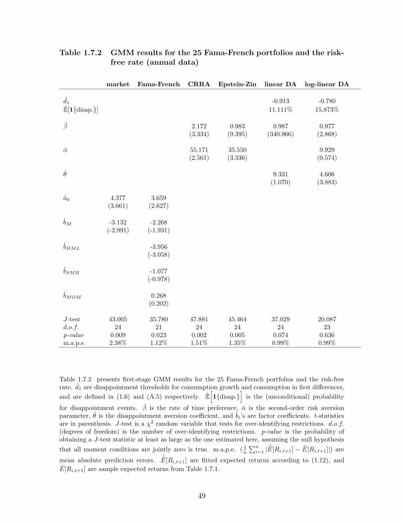
Table 1.7.2 GMM results for the 25 Fama-French portfolios and the risk-free rate (annual data)

market Fama-French CRRA Epstein-Zin linear DA log-linear DA

d1 -0.913 -0.780

E[1{disap.}] 11.111% 15.873%

β 2.172 0.983 0.987 0.977(3.334) (9.395) (340.966) (2.868)

α 55.171 35.550 9.929(2.561) (3.336) (0.574)

θ 9.331 4.606(1.070) (3.883)

a0 4.377 3.659(3.661) (2.627)

bM -3.132 -2.268(-2.991) (-1.931)

bHML -3.956(-3.058)

bSMB -1.077(-0.978)

bMOM 0.268(0.202)

J-test 43.005 35.780 47.881 45.464 37.029 20.087d.o.f. 24 21 24 24 24 23p-value 0.009 0.023 0.002 0.005 0.074 0.636m.a.p.e. 2.38% 1.12% 1.51% 1.35% 0.99% 0.99%

Table 1.7.2 presents first-stage GMM results for the 25 Fama-French portfolios and the risk-freerate. d1 are disappointment thresholds for consumption growth and consumption in first differences,

and are defined in (1.6) and (A.5) respectively. E[1{disap.}

]is the (unconditional) probability

for disappointment events. β is the rate of time preference, α is the second-order risk aversionparameter, θ is the disappointment aversion coefficient, and bi’s are factor coefficients. t-statisticsare in parenthesis. J-test is a χ2 random variable that tests for over-identifying restrictions. d.o.f.(degrees of freedom) is the number of over-identifying restrictions. p-value is the probability ofobtaining a J-test statistic at least as large as the one estimated here, assuming the null hypothesis

that all moment conditions are jointly zero is true. m.a.p.e. ( 1n

∑ni=1 |

ˆE[Ri,t+1] − E[Ri,t+1]|) are

mean absolute prediction errors.ˆE[Ri,t+1] are fitted expected returns according to (1.12), and

E[Ri,t+1] are sample expected returns from Table 1.7.1.

49

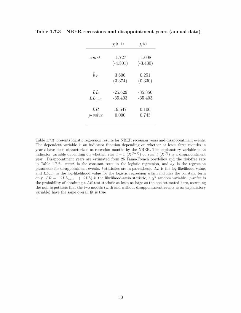
Table 1.7.3 NBER recessions and disappointment years (annual data)

X(t−1) X(t)

const. -1.727 -1.098(-4.501) (-3.430)

bX 3.806 0.251(3.374) (0.330)

LL -25.629 -35.350LLnull -35.403 -35.403

LR 19.547 0.106p-value 0.000 0.743

Table 1.7.3 presents logistic regression results for NBER recession years and disappointment events.The dependent variable is an indicator function depending on whether at least three months inyear t have been characterized as recession months by the NBER. The explanatory variable is anindicator variable depending on whether year t − 1 (X(t−1)) or year t (X(t)) is a disappointmentyear. Disappointment years are estimated from 25 Fama-French portfolios and the risk-free ratein Table 1.7.2. const. is the constant term in the logistic regression, and bX is the regressionparameter for disappointment events. t-statistics are in parenthesis. LL is the log-likelihood value,and LLnull is the log-likelihood value for the logistic regression which includes the constant termonly. LR = −2LLnull − (−2LL) is the likelihood-ratio statistic, a χ2 random variable. p-value isthe probability of obtaining a LR-test statistic at least as large as the one estimated here, assumingthe null hypothesis that the two models (with and without disappointment events as an explanatoryvariable) have the same overall fit is true

.

50

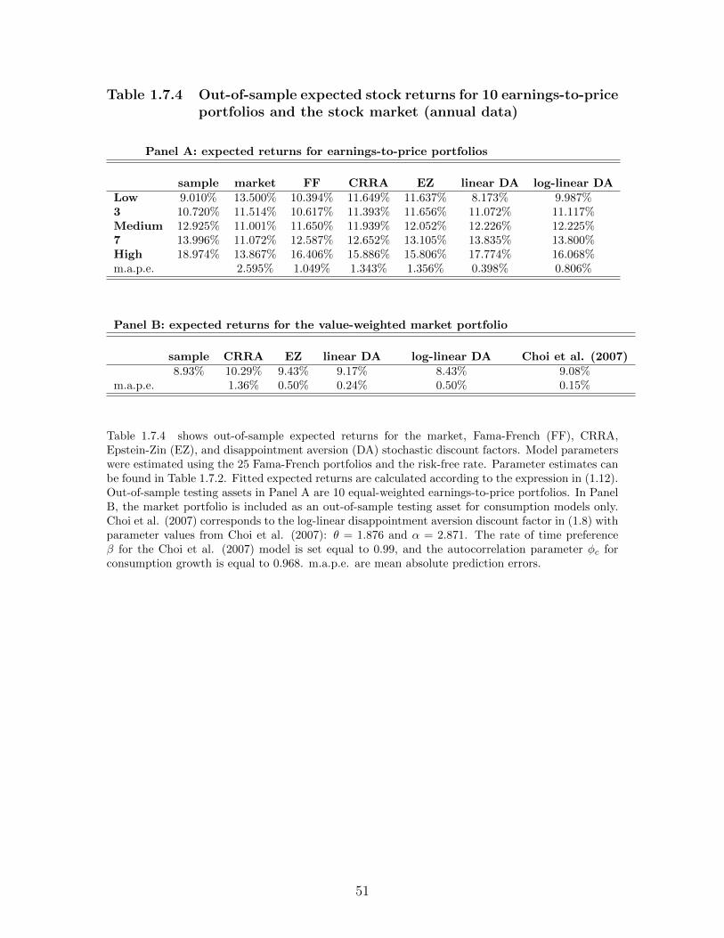
Table 1.7.4 Out-of-sample expected stock returns for 10 earnings-to-priceportfolios and the stock market (annual data)

Panel A: expected returns for earnings-to-price portfolios

sample market FF CRRA EZ linear DA log-linear DALow 9.010% 13.500% 10.394% 11.649% 11.637% 8.173% 9.987%3 10.720% 11.514% 10.617% 11.393% 11.656% 11.072% 11.117%Medium 12.925% 11.001% 11.650% 11.939% 12.052% 12.226% 12.225%7 13.996% 11.072% 12.587% 12.652% 13.105% 13.835% 13.800%High 18.974% 13.867% 16.406% 15.886% 15.806% 17.774% 16.068%m.a.p.e. 2.595% 1.049% 1.343% 1.356% 0.398% 0.806%

Panel B: expected returns for the value-weighted market portfolio

sample CRRA EZ linear DA log-linear DA Choi et al. (2007)8.93% 10.29% 9.43% 9.17% 8.43% 9.08%

m.a.p.e. 1.36% 0.50% 0.24% 0.50% 0.15%

Table 1.7.4 shows out-of-sample expected returns for the market, Fama-French (FF), CRRA,Epstein-Zin (EZ), and disappointment aversion (DA) stochastic discount factors. Model parameterswere estimated using the 25 Fama-French portfolios and the risk-free rate. Parameter estimates canbe found in Table 1.7.2. Fitted expected returns are calculated according to the expression in (1.12).Out-of-sample testing assets in Panel A are 10 equal-weighted earnings-to-price portfolios. In PanelB, the market portfolio is included as an out-of-sample testing asset for consumption models only.Choi et al. (2007) corresponds to the log-linear disappointment aversion discount factor in (1.8) withparameter values from Choi et al. (2007): θ = 1.876 and α = 2.871. The rate of time preferenceβ for the Choi et al. (2007) model is set equal to 0.99, and the autocorrelation parameter φc forconsumption growth is equal to 0.968. m.a.p.e. are mean absolute prediction errors.

51

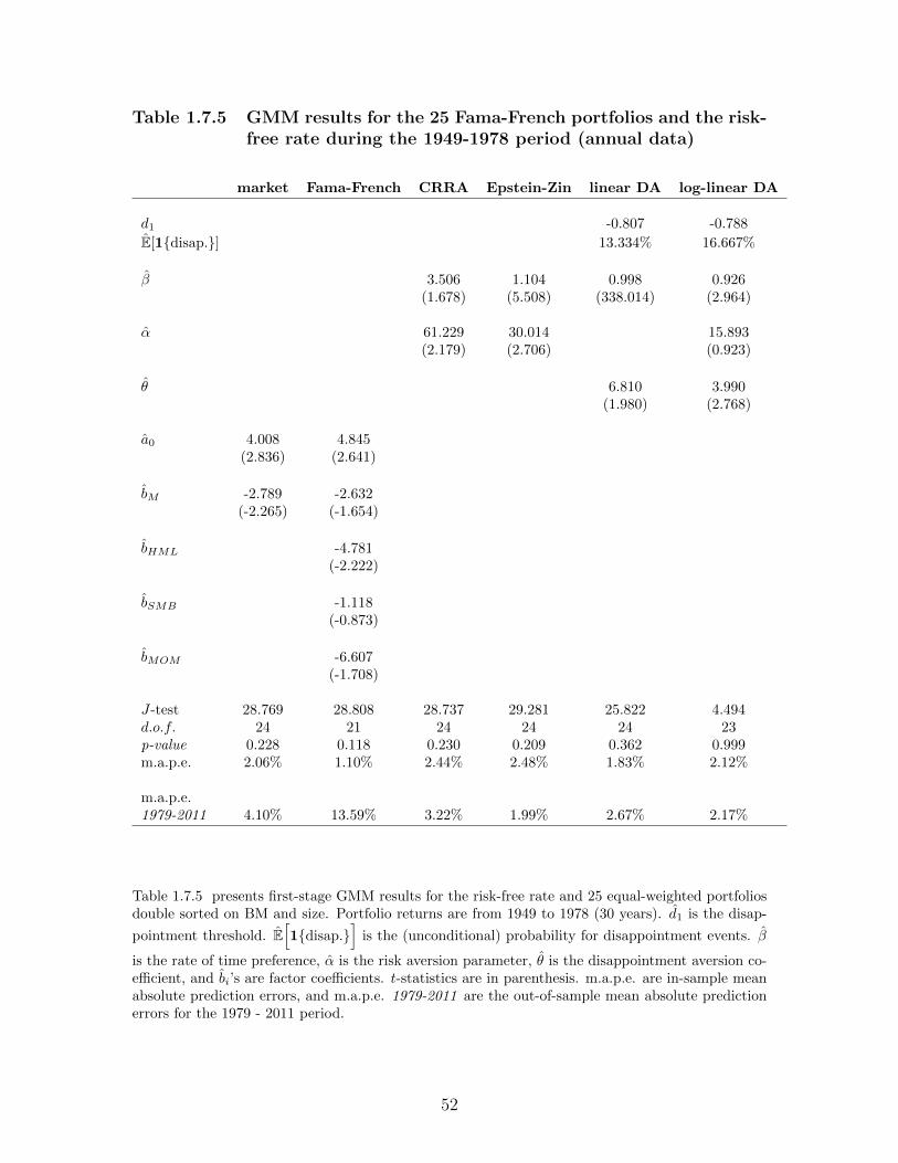
Table 1.7.5 GMM results for the 25 Fama-French portfolios and the risk-free rate during the 1949-1978 period (annual data)

market Fama-French CRRA Epstein-Zin linear DA log-linear DA

d1 -0.807 -0.788

E[1{disap.}] 13.334% 16.667%

β 3.506 1.104 0.998 0.926(1.678) (5.508) (338.014) (2.964)

α 61.229 30.014 15.893(2.179) (2.706) (0.923)

θ 6.810 3.990(1.980) (2.768)

a0 4.008 4.845(2.836) (2.641)

bM -2.789 -2.632(-2.265) (-1.654)

bHML -4.781(-2.222)

bSMB -1.118(-0.873)

bMOM -6.607(-1.708)

J-test 28.769 28.808 28.737 29.281 25.822 4.494d.o.f. 24 21 24 24 24 23p-value 0.228 0.118 0.230 0.209 0.362 0.999m.a.p.e. 2.06% 1.10% 2.44% 2.48% 1.83% 2.12%

m.a.p.e.1979-2011 4.10% 13.59% 3.22% 1.99% 2.67% 2.17%

Table 1.7.5 presents first-stage GMM results for the risk-free rate and 25 equal-weighted portfoliosdouble sorted on BM and size. Portfolio returns are from 1949 to 1978 (30 years). d1 is the disap-

pointment threshold. E[1{disap.}

]is the (unconditional) probability for disappointment events. β

is the rate of time preference, α is the risk aversion parameter, θ is the disappointment aversion co-efficient, and bi’s are factor coefficients. t-statistics are in parenthesis. m.a.p.e. are in-sample meanabsolute prediction errors, and m.a.p.e. 1979-2011 are the out-of-sample mean absolute predictionerrors for the 1979 - 2011 period.

52

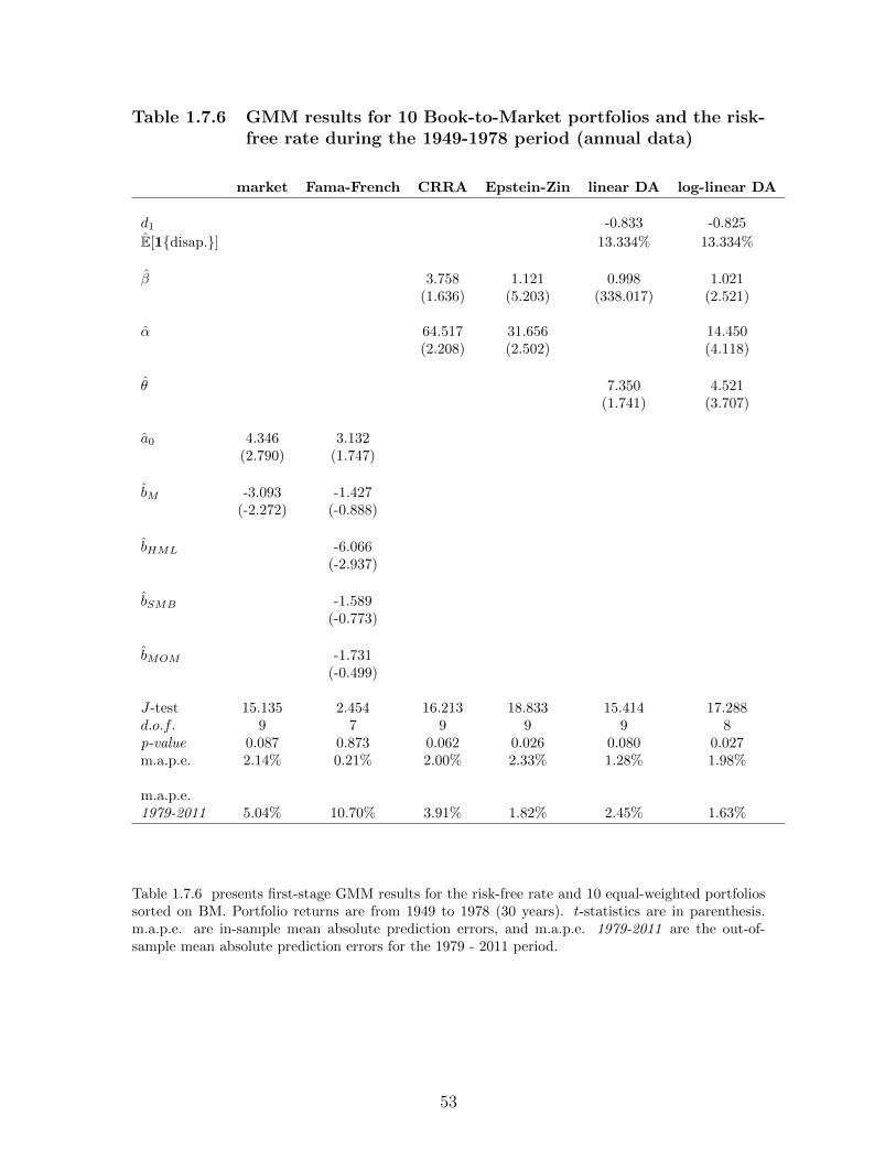
Table 1.7.6 GMM results for 10 Book-to-Market portfolios and the risk-free rate during the 1949-1978 period (annual data)

market Fama-French CRRA Epstein-Zin linear DA log-linear DA

d1 -0.833 -0.825

E[1{disap.}] 13.334% 13.334%

β 3.758 1.121 0.998 1.021(1.636) (5.203) (338.017) (2.521)

α 64.517 31.656 14.450(2.208) (2.502) (4.118)

θ 7.350 4.521(1.741) (3.707)

a0 4.346 3.132(2.790) (1.747)

bM -3.093 -1.427(-2.272) (-0.888)

bHML -6.066(-2.937)

bSMB -1.589(-0.773)

bMOM -1.731(-0.499)

J-test 15.135 2.454 16.213 18.833 15.414 17.288d.o.f. 9 7 9 9 9 8p-value 0.087 0.873 0.062 0.026 0.080 0.027m.a.p.e. 2.14% 0.21% 2.00% 2.33% 1.28% 1.98%

m.a.p.e.1979-2011 5.04% 10.70% 3.91% 1.82% 2.45% 1.63%

Table 1.7.6 presents first-stage GMM results for the risk-free rate and 10 equal-weighted portfoliossorted on BM. Portfolio returns are from 1949 to 1978 (30 years). t-statistics are in parenthesis.m.a.p.e. are in-sample mean absolute prediction errors, and m.a.p.e. 1979-2011 are the out-of-sample mean absolute prediction errors for the 1979 - 2011 period.

53

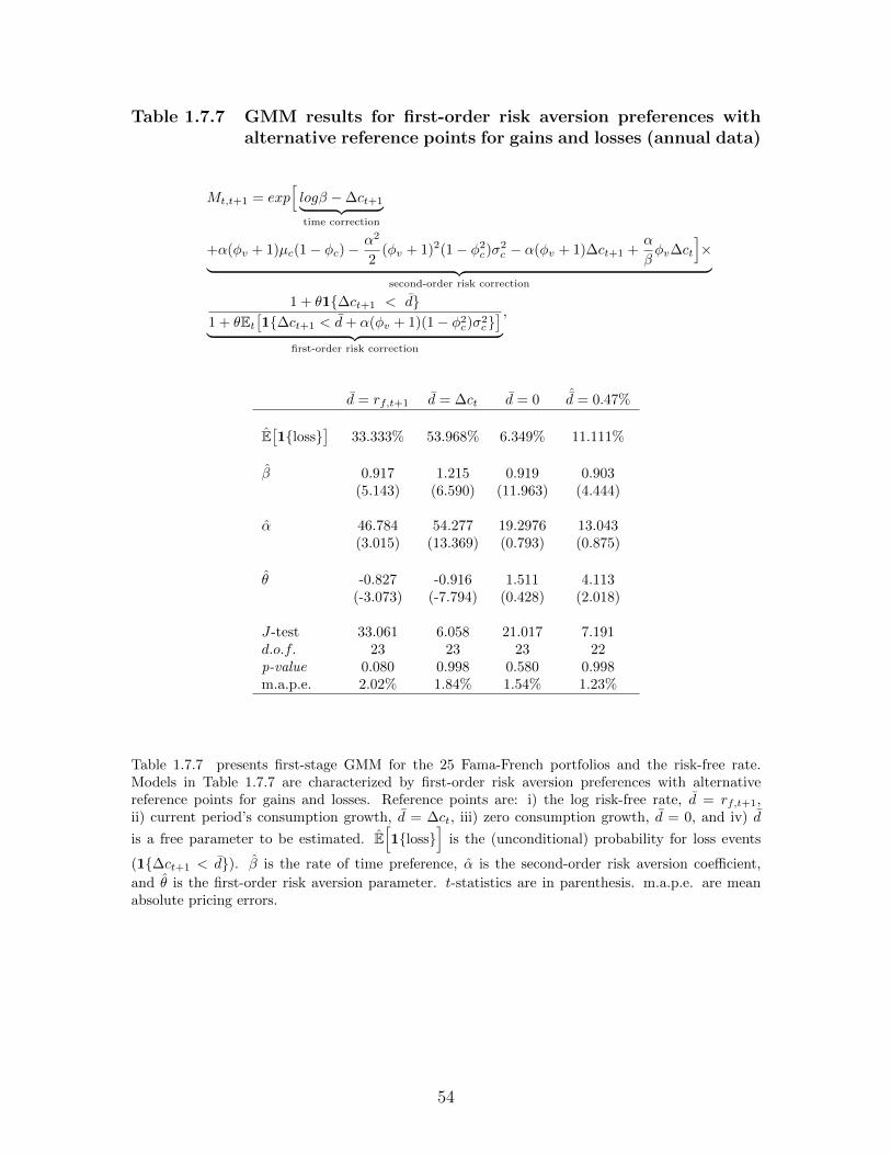
Table 1.7.7 GMM results for first-order risk aversion preferences withalternative reference points for gains and losses (annual data)

Mt,t+1 = exp[logβ −∆ct+1︸ ︷︷ ︸time correction

+α(φv + 1)µc(1− φc)−α2

2(φv + 1)2(1− φ2

c)σ2c − α(φv + 1)∆ct+1 +

α

βφv∆ct

]×︸ ︷︷ ︸

second-order risk correction

1 + θ1{∆ct+1 < d}1 + θEt

[1{∆ct+1 < d+ α(φv + 1)(1− φ2

c)σ2c}]︸ ︷︷ ︸

first-order risk correction

,

d = rf,t+1 d = ∆ct d = 0 ˆd = 0.47%

E[1{loss}

]33.333% 53.968% 6.349% 11.111%

β 0.917 1.215 0.919 0.903(5.143) (6.590) (11.963) (4.444)

α 46.784 54.277 19.2976 13.043(3.015) (13.369) (0.793) (0.875)

θ -0.827 -0.916 1.511 4.113(-3.073) (-7.794) (0.428) (2.018)

J-test 33.061 6.058 21.017 7.191d.o.f. 23 23 23 22p-value 0.080 0.998 0.580 0.998m.a.p.e. 2.02% 1.84% 1.54% 1.23%

Table 1.7.7 presents first-stage GMM for the 25 Fama-French portfolios and the risk-free rate.Models in Table 1.7.7 are characterized by first-order risk aversion preferences with alternativereference points for gains and losses. Reference points are: i) the log risk-free rate, d = rf,t+1,ii) current period’s consumption growth, d = ∆ct, iii) zero consumption growth, d = 0, and iv) d

is a free parameter to be estimated. E[1{loss}

]is the (unconditional) probability for loss events

(1{∆ct+1 < d}). β is the rate of time preference, α is the second-order risk aversion coefficient,

and θ is the first-order risk aversion parameter. t-statistics are in parenthesis. m.a.p.e. are meanabsolute pricing errors.

54

Table 1.7.8 GMM results for the 25 Fama-French portfolios and the risk-free rate (quarterly data)

market Fama-French CRRA Epstein-Zin linear DA log-linear DA

d1 -0.858 -0.774

E[1{disap.}] 15.294% 16.862%

β 1.483 0.917 0.997 0.996(13.030) (5.110) (2,486) (4.173)

α 138.538 147.910 14.376(3.368) (1.406) (0.352)

θ 7.932 5.274(1.412) (2.861)

a0 4.317 6.892(4.342) (4.296)

bM -3.253 -5.406(-3.392) (-3.604)

bHML -8.625(-4.527)

bSMB -4.534(-1.865)

bMOM -11.055(-2.227)

J-test 78.741 43.351 71.640 70.984 35.234 8.921d.o.f. 24 21 24 24 24 23p-value 0.000 0.002 0.000 0.000 0.065 0.996m.a.p.e. 0.60% 0.24% 0.40% 0.48% 0.43% 0.42%

Table 1.7.8 presents first-stage GMM results for the 25 Fama-French portfolios and the risk-freerate at the quarterly frequency.

55

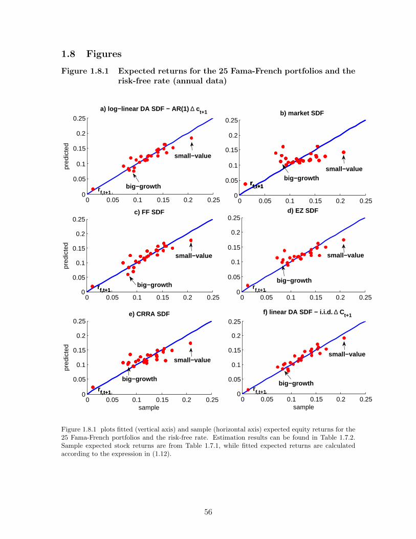
1.8 Figures

Figure 1.8.1 Expected returns for the 25 Fama-French portfolios and therisk-free rate (annual data)

0 0.05 0.1 0.15 0.2 0.250

0.05

0.1

0.15

0.2

0.25

sample

f) linear DA SDF − i.i.d. ∆ Ct+1

small−value

big−growthrf,t+1

0 0.05 0.1 0.15 0.2 0.250

0.05

0.1

0.15

0.2

0.25

pred

icte

d

a) log−linear DA SDF − AR(1) ∆ ct+1

small−value

big−growthrf,t+1

0 0.05 0.1 0.15 0.2 0.250

0.05

0.1

0.15

0.2

0.25

sample

pred

icte

d

e) CRRA SDF

rf,t+1

small−value

big−growth

rf,t+1

0 0.05 0.1 0.15 0.2 0.250

0.05

0.1

0.15

0.2

0.25

pred

icte

d

c) FF SDF

rf,t+1

small−value

big−growthrf,t+1

0 0.05 0.1 0.15 0.2 0.250

0.05

0.1

0.15

0.2

0.25b) market SDF

rf,t+1rf,t+1

small−valuebig−growth

rf,t+1

0 0.05 0.1 0.15 0.2 0.250

0.05

0.1

0.15

0.2

0.25d) EZ SDF

small−value

big−growthrf,t+1

Student Version of MATLAB

Figure 1.8.1 plots fitted (vertical axis) and sample (horizontal axis) expected equity returns for the25 Fama-French portfolios and the risk-free rate. Estimation results can be found in Table 1.7.2.Sample expected stock returns are from Table 1.7.1, while fitted expected returns are calculatedaccording to the expression in (1.12).

56

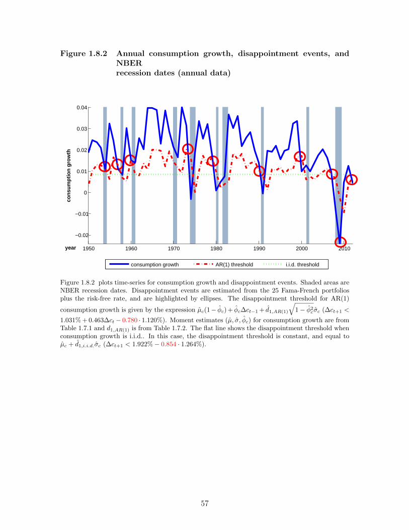
Figure 1.8.2 Annual consumption growth, disappointment events, andNBERrecession dates (annual data)

year

con

sum

pti

on

gro

wth

1950 1960 1970 1980 1990 2000 2010

−0.02

−0.01

0

0.01

0.02

0.03

0.04

consumption growth AR(1) threshold i.i.d. threshold

Student Version of MATLAB

Figure 1.8.2 plots time-series for consumption growth and disappointment events. Shaded areas areNBER recession dates. Disappointment events are estimated from the 25 Fama-French portfoliosplus the risk-free rate, and are highlighted by ellipses. The disappointment threshold for AR(1)

consumption growth is given by the expression µc(1− φc) + φc∆ct−1 + d1,AR(1)

√1− φ2

c σc (∆ct+1 <

1.031% + 0.463∆ct − 0.780 · 1.120%). Moment estimates (µ, σ, φc) for consumption growth are fromTable 1.7.1 and d1,AR(1) is from Table 1.7.2. The flat line shows the disappointment threshold whenconsumption growth is i.i.d.. In this case, the disappointment threshold is constant, and equal toµc + d1,i.i.d.σc (∆ct+1 < 1.922%− 0.854 · 1.264%).

57

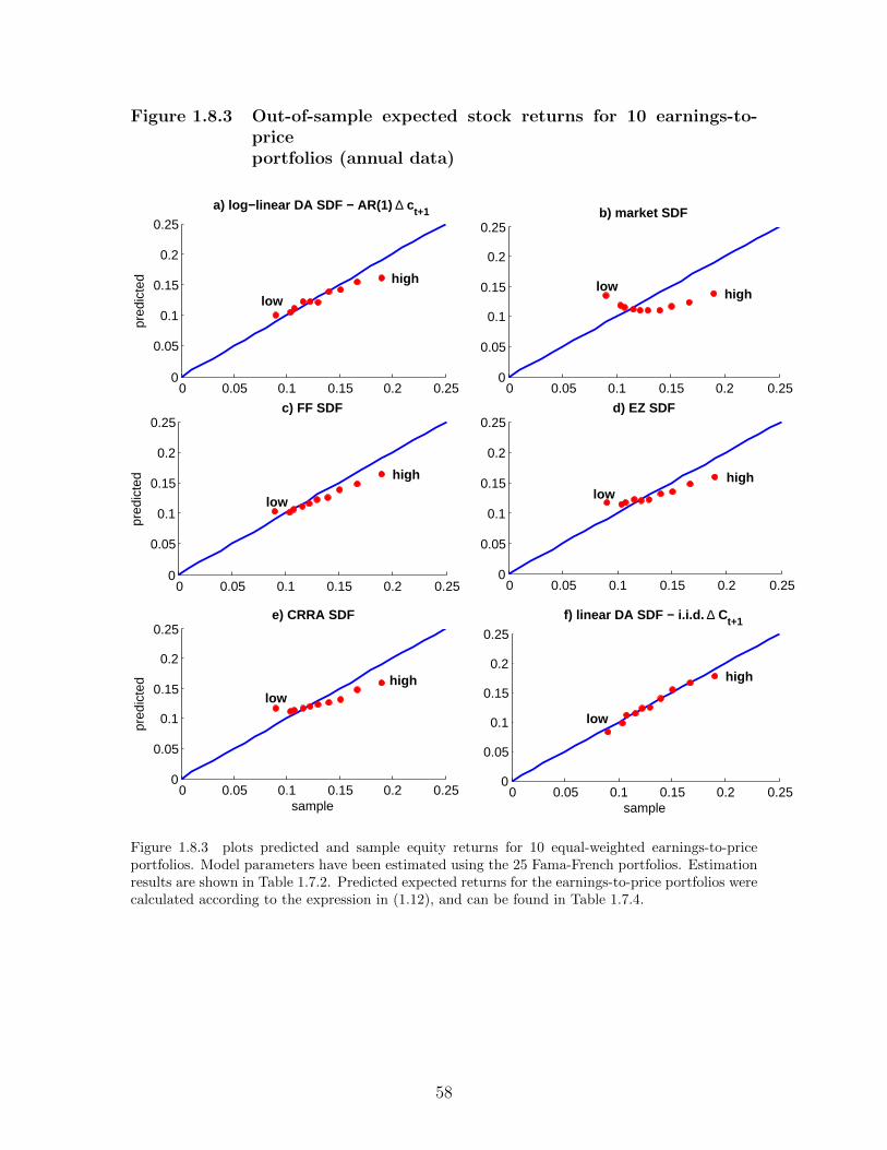
Figure 1.8.3 Out-of-sample expected stock returns for 10 earnings-to-priceportfolios (annual data)

0 0.05 0.1 0.15 0.2 0.250

0.05

0.1

0.15

0.2

0.25

pred

icte

d

c) FF SDF

low

high

0 0.05 0.1 0.15 0.2 0.250

0.05

0.1

0.15

0.2

0.25b) market SDF

lowhigh

0 0.05 0.1 0.15 0.2 0.250

0.05

0.1

0.15

0.2

0.25

sample

pred

icte

d

e) CRRA SDF

lowhigh

0 0.05 0.1 0.15 0.2 0.250

0.05

0.1

0.15

0.2

0.25d) EZ SDF

lowhigh

0 0.05 0.1 0.15 0.2 0.250

0.05

0.1

0.15

0.2

0.25

sample

f) linear DA SDF − i.i.d. ∆ Ct+1

low

high

0 0.05 0.1 0.15 0.2 0.250

0.05

0.1

0.15

0.2

0.25

pred

icte

d

a) log−linear DA SDF − AR(1) ∆ ct+1

low

high

Student Version of MATLAB

Figure 1.8.3 plots predicted and sample equity returns for 10 equal-weighted earnings-to-priceportfolios. Model parameters have been estimated using the 25 Fama-French portfolios. Estimationresults are shown in Table 1.7.2. Predicted expected returns for the earnings-to-price portfolios werecalculated according to the expression in (1.12), and can be found in Table 1.7.4.

58

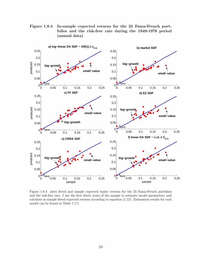
Figure 1.8.4 In-sample expected returns for the 25 Fama-French port-folios and the risk-free rate during the 1949-1978 period(annual data)

0 0.05 0.1 0.15 0.2 0.250

0.05

0.1

0.15

0.2

0.25

pred

icte

d

a) log−linear DA SDF − AR(1) ∆ ct+1

small−value

big−growth

rf,t+1

0 0.05 0.1 0.15 0.2 0.250

0.05

0.1

0.15

0.2

0.25

sample

f) linear DA SDF − i.i.d. ∆ Ct+1

small−valuebig−growth

rf,t+1

0 0.05 0.1 0.15 0.2 0.250

0.05

0.1

0.15

0.2

0.25d) EZ SDF

small−value

big−growth

rf,t+1

0 0.05 0.1 0.15 0.2 0.250

0.05

0.1

0.15

0.2

0.25

pred

icte

d

c) FF SDF

small−value

big−growth

rf,t+1

0 0.05 0.1 0.15 0.2 0.250

0.05

0.1

0.15

0.2

0.25b) market SDF

small−value

big−growth

rf,t+1

0 0.05 0.1 0.15 0.2 0.250

0.05

0.1

0.15

0.2

0.25

sample

pred

icte

d

e) CRRA SDF

small−valuebig−growth

rf,t+1

Student Version of MATLAB

Figure 1.8.4 plots fitted and sample expected equity returns for the 25 Fama-French portfoliosand the risk-free rate. I use the first thirty years of the sample to estimate model parameters, andcalculate in-sample fitted expected returns according to equation (1.12). Estimation results for eachmodel can be found in Table 1.7.5.

59

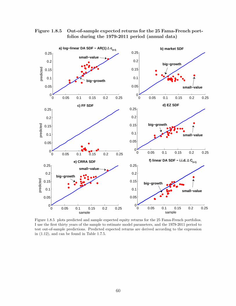
Figure 1.8.5 Out-of-sample expected returns for the 25 Fama-French port-folios during the 1979-2011 period (annual data)

0 0.05 0.1 0.15 0.2 0.250

0.05

0.1

0.15

0.2

0.25

pred

icte

d

a) log−linear DA SDF − AR(1) ∆ ct+1

small−value

big−growth

0 0.05 0.1 0.15 0.2 0.250

0.05

0.1

0.15

0.2

0.25

sample

f) linear DA SDF − i.i.d. ∆ Ct+1

big−growth

small−value

0 0.05 0.1 0.15 0.2 0.250

0.05

0.1

0.15

0.2

0.25b) market SDF

small−value

big−growth

0 0.05 0.1 0.15 0.2 0.250

0.05

0.1

0.15

0.2

0.25

pred

icte

d

c) FF SDF

0 0.05 0.1 0.15 0.2 0.250

0.05

0.1

0.15

0.2

0.25

sample

pred

icte

d

e) CRRA SDF

small−value

big−growth

0 0.05 0.1 0.15 0.2 0.250

0.05

0.1

0.15

0.2

0.25d) EZ SDF

small−value

big−growth

Student Version of MATLAB

Figure 1.8.5 plots predicted and sample expected equity returns for the 25 Fama-French portfolios.I use the first thirty years of the sample to estimate model parameters, and the 1979-2011 period totest out-of-sample predictions. Predicted expected returns are derived according to the expressionin (1.12), and can be found in Table 1.7.5.

60

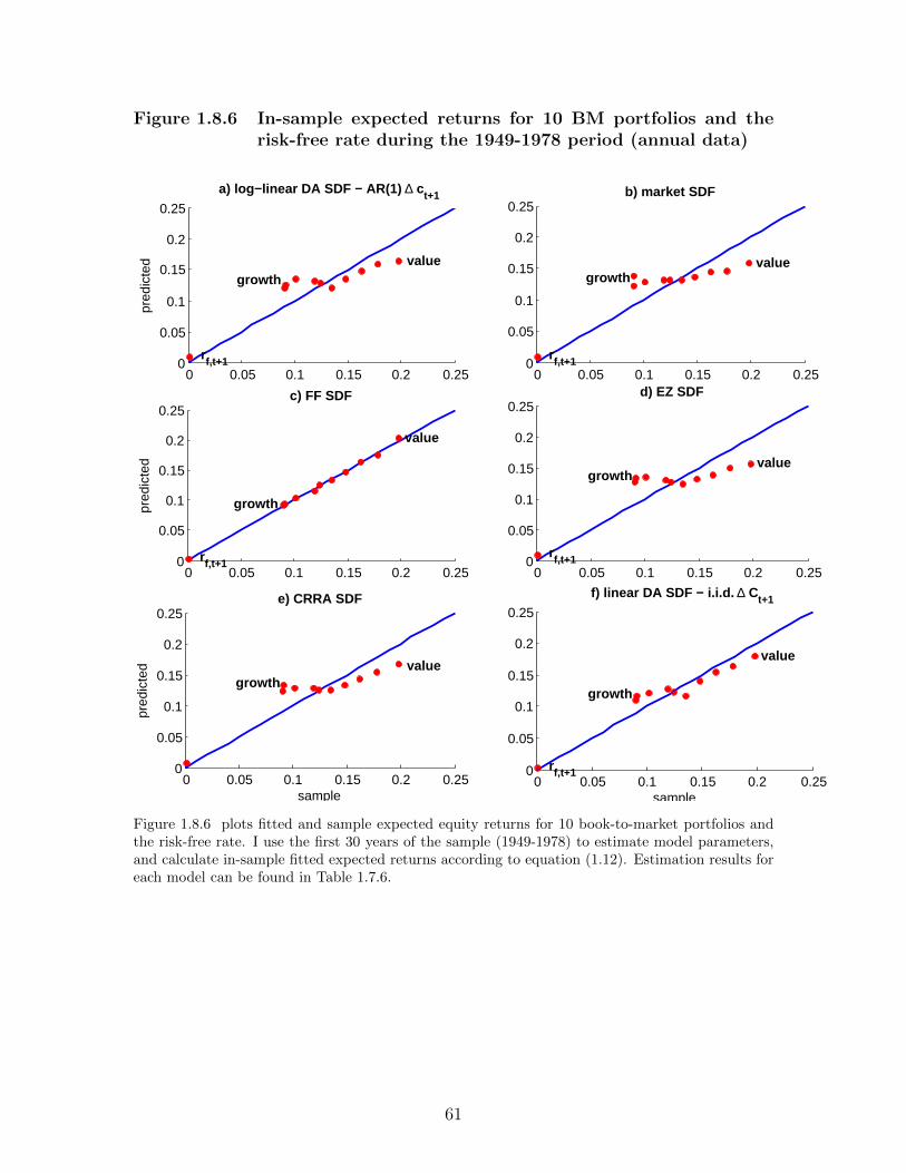
Figure 1.8.6 In-sample expected returns for 10 BM portfolios and therisk-free rate during the 1949-1978 period (annual data)

0 0.05 0.1 0.15 0.2 0.250

0.05

0.1

0.15

0.2

0.25b) market SDF

growthvalue

rf,t+1

0 0.05 0.1 0.15 0.2 0.250

0.05

0.1

0.15

0.2

0.25

pred

icte

d

c) FF SDF

growth

value

rf,t+10 0.05 0.1 0.15 0.2 0.25

0

0.05

0.1

0.15

0.2

0.25d) EZ SDF

growthvalue

rf,t+1

0 0.05 0.1 0.15 0.2 0.250

0.05

0.1

0.15

0.2

0.25

pred

icte

d

a) log−linear DA SDF − AR(1) ∆ ct+1

growthvalue

rf,t+1

0 0.05 0.1 0.15 0.2 0.250

0.05

0.1

0.15

0.2

0.25

sample

f) linear DA SDF − i.i.d. ∆ Ct+1

growth

value

rf,t+10 0.05 0.1 0.15 0.2 0.25

0

0.05

0.1

0.15

0.2

0.25

sample

pred

icte

d

e) CRRA SDF

growthvalue

Student Version of MATLAB

Figure 1.8.6 plots fitted and sample expected equity returns for 10 book-to-market portfolios andthe risk-free rate. I use the first 30 years of the sample (1949-1978) to estimate model parameters,and calculate in-sample fitted expected returns according to equation (1.12). Estimation results foreach model can be found in Table 1.7.6.

61

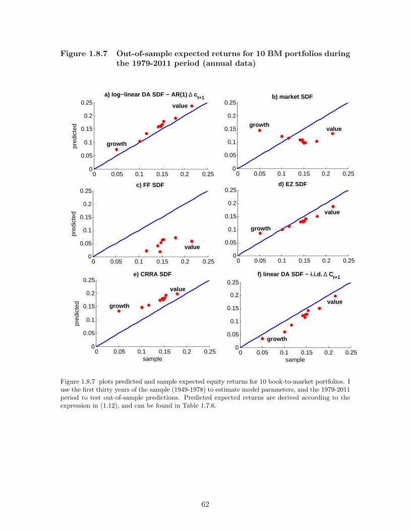
Figure 1.8.7 Out-of-sample expected returns for 10 BM portfolios duringthe 1979-2011 period (annual data)

0 0.05 0.1 0.15 0.2 0.250

0.05

0.1

0.15

0.2

0.25b) market SDF

growthvalue

0 0.05 0.1 0.15 0.2 0.250

0.05

0.1

0.15

0.2

0.25

pred

icte

d

c) FF SDF

value

0 0.05 0.1 0.15 0.2 0.250

0.05

0.1

0.15

0.2

0.25d) EZ SDF

growth

value

0 0.05 0.1 0.15 0.2 0.250

0.05

0.1

0.15

0.2

0.25

pred

icte

d

a) log−linear DA SDF − AR(1) ∆ ct+1

growth

value

0 0.05 0.1 0.15 0.2 0.250

0.05

0.1

0.15

0.2

0.25

sample

f) linear DA SDF − i.i.d. ∆ Ct+1

growth

value

0 0.05 0.1 0.15 0.2 0.250

0.05

0.1

0.15

0.2

0.25

sample

pred

icte

d

e) CRRA SDF

growth

value

Student Version of MATLAB

Figure 1.8.7 plots predicted and sample expected equity returns for 10 book-to-market portfolios. Iuse the first thirty years of the sample (1949-1978) to estimate model parameters, and the 1979-2011period to test out-of-sample predictions. Predicted expected returns are derived according to theexpression in (1.12), and can be found in Table 1.7.6.

62

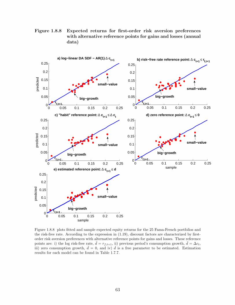
Figure 1.8.8 Expected returns for first-order risk aversion preferenceswith alternative reference points for gains and losses (annualdata)

0 0.05 0.1 0.15 0.2 0.250

0.05

0.1

0.15

0.2

0.25

e) estimated reference point: ∆ ct+1 ≤ d

rf,t+1

sample

pred

icte

d

small−value

big−growth

0 0.05 0.1 0.15 0.2 0.250

0.05

0.1

0.15

0.2

0.25

b) risk−free rate reference point: ∆ ct+1 ≤ rf,t+1

small−value

big−growth

rf,t+1

0 0.05 0.1 0.15 0.2 0.250

0.05

0.1

0.15

0.2

0.25

pred

icte

d

c) "habit" reference point: ∆ ct+1 ≤ ∆ ct

small−value

big−growthrf,t+1

0 0.05 0.1 0.15 0.2 0.250

0.05

0.1

0.15

0.2

0.25

sample

d) zero reference point: ∆ ct+1 ≤ 0

small−value

big−growthrf,t+1

0 0.05 0.1 0.15 0.2 0.250

0.05

0.1

0.15

0.2

0.25

pred

icte

d

a) log−linear DA SDF − AR(1) ∆ ct+1

small−value

big−growthrf,t+1

Student Version of MATLAB

Figure 1.8.8 plots fitted and sample expected equity returns for the 25 Fama-French portfolios andthe risk-free rate. According to the expression in (1.19), discount factors are characterized by first-order risk aversion preferences with alternative reference points for gains and losses. These referencepoints are: i) the log risk-free rate, d = rf,t+1, ii) previous period’s consumption growth, d = ∆ct,iii) zero consumption growth, d = 0, and iv) d is a free parameter to be estimated. Estimationresults for each model can be found in Table 1.7.7.

63

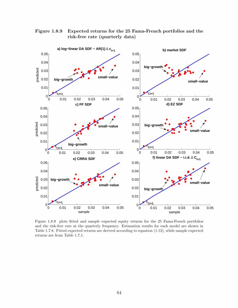
Figure 1.8.9 Expected returns for the 25 Fama-French portfolios and therisk-free rate (quarterly data)

0 0.01 0.02 0.03 0.04 0.050

0.01

0.02

0.03

0.04

0.05

sample

f) linear DA SDF − i.i.d. ∆ Ct+1

small−value

big−growth

rf,t+1

0 0.01 0.02 0.03 0.04 0.050

0.01

0.02

0.03

0.04

0.05d) EZ SDF

small−value

big−growth

rf,t+1

0 0.01 0.02 0.03 0.04 0.050

0.01

0.02

0.03

0.04

0.05

pred

icte

d

a) log−linear DA SDF − AR(1) ∆ ct+1

small−valuebig−growth

rf,t+1

0 0.01 0.02 0.03 0.04 0.050

0.01

0.02

0.03

0.04

0.05

sample

pred

icte

d

e) CRRA SDF

small−value

big−growth

rf,t+1

0 0.01 0.02 0.03 0.04 0.050

0.01

0.02

0.03

0.04

0.05

pred

icte

d

c) FF SDF

small−value

big−growthrf,t+1

0 0.01 0.02 0.03 0.04 0.050

0.01

0.02

0.03

0.04

0.05b) market SDF

small−value

big−growth

rf,t+1

Student Version of MATLAB

Figure 1.8.9 plots fitted and sample expected equity returns for the 25 Fama-French portfoliosand the risk-free rate at the quarterly frequency. Estimation results for each model are shown inTable 1.7.8. Fitted expected returns are derived according to equation (1.12), while sample expectedreturns are from Table 1.7.1.

64

CHAPTER II

Disappointment Aversion Preferences, and the

Credit Spread Puzzle

oυκ αν λαβoις παρα τoυ µη εχoντoς

“You cannot receive anything by someone who has nothing”

“Dialogues of the Dead”, Lucian (125− 175 A.D.)

2.1 Abstract

Structural models of default are unable to generate measurable Baa-Aaa credit

spreads, when these models are calibrated to realistic values for default rates and

losses given default. Motivated by recent results in behavioral economics, this paper

is the first to propose a consumption-based asset pricing model with disappointment

aversion preferences in an attempt to resolve the credit spread puzzle. Simulation

results suggest that as long as losses given default and default boundaries are coun-

tercyclical, then the disappointment model can explain Baa-Aaa credit spreads using

preference parameters that are consistent with experimental findings. Further, the

disappointment aversion discount factor can match key moments for stock market

returns, the price-dividend ratio, and the risk-free rate.

65

2.2 Introduction

When traditional structural models of default1 are calibrated to realistic values

for default rates and losses given default, then these models are unable to generate

measurable Baa-Aaa credit spreads, an empirical conundrum also known as the credit

spread puzzle. Moreover, recent results2 suggest that state-of-the-art consumption-

based asset pricing models cannot rationalize corporate bond spreads, even if they are

successful in explaining equity premia. Nevertheless, a universal stochastic discount

that can resolve the equity premium puzzle should also be able to fit credit spreads

in corporate bond markets.

Although behavioral theories have been extensively used to explain equity risk pre-

mia3, this is the first paper to address the credit spread puzzle from a behavioral per-

spective. Towards this objective, I use a general equilibrium model of an endowment

economy populated by disappointment averse investors in order to price zero-coupon

corporate bonds subject to default. Disappointment aversion preferences were first

introduced by Gul (1991), and are able to capture well documented patterns for risky

choices, such as asymmetric marginal utility over gains and losses or reference-based

evaluation of stochastic payoffs4, without violating first-order stochastic dominance,

transitivity of preferences or aggregation of investors. The disappointment aversion

framework can therefore help us shed additional light on the link between credit-

spreads and aggregate economic activity while maintaining investor rationality.

Disappointment averse investors are characterized by first-order risk aversion5

preferences with endogenous expectation-based reference points for gains and losses.

Due to the linear homogeneity of these preferences, I am able to obtain approximate

1e.g. Merton (1974)2Chen et al. 2009.3Epstein and Zin (1990), Bernatzi and Thaler (1995), Barberis et al. (2001), Andries (2011),

Piccioni (2011), Easley and Yang (2012), Delikouras (2013).4Kahneman and Tversky (1979), Duncan (2010), Pope and Schweitzer (2011).5Segal and Spivak (1990).

66

analytical solutions for the price-payout ratios in the economy which are log-linear

functions of three state variables: consumption growth, consumption growth volatil-

ity, and consumption growth variance. Explicit solutions for price-payout ratios, in

turn, facilitate the simulation algorithm, and provide valuable intuition. The main

mechanism in place for disappointment aversion preferences is related to asymmetric

marginal utility, and the fact that disappointment averse investors penalize losses

below the endogenous reference level three times more than they do for losses above

the reference level.

The disappointment aversion model highlights the interaction between default

rates and periods of worse-than-expected aggregate macroeconomic conditions when

marginal utility is high. During these periods there is an upwards jump in marginal

utility. Almeida and Philipon (2007) also document that distress costs are most likely

to happen during times when marginal utility is high. Figure 2.9.1 shows Baa-Aaa

credit spreads, Baa default rates, and NBER recessions for the 1946-2011 period.

Two things become immediately clear from Figure 2.9.1. First, credit spreads are

strongly countercyclical. Second, Baa default rates are zero during most of the time,

and tend to spike up at or after a recession. Through first-order risk aversion, the

disappointment model amplifies very small risks, such as the almost zero default risk

for Baa firms, and is able to generate measurable Baa-Aaa credit spreads despite the

very low default rates.

Although several consumption-based asset pricing models have proposed frame-

works that generate credit spreads consistent with empirical observations, with the

exception of the habit model in Chen et al. (2009), either preference parameters (eg.

the risk aversion coefficient) in these models are much larger than those estimated

in clinical experiments6, or these models cannot perfectly match other asset pricing

6Chen (2010), p. 2190, assumes a risk aversion parameter equal to 6.5 and an EIS larger than1. Bhamra et al. (2010) remain silent on preference parameters, and focus on risk-neutral pricing.

67

moments such as equity risk premia7. On the other hand, preference parameters for

the disappointment model in this paper are calibrated to values which are consistent

with recent experimental results8: the risk aversion parameter is equal to 1.8, and the

disappointment aversion coefficient is equal to 2.03.

By providing evidence that the disappointment model can contribute to the reso-

lution of the credit spread puzzle, this paper compliments a growing literature which

argues that disappointment aversion preferences are able address a variety of stylized

facts in financial markets such as the equity premium puzzle (Routledge and Zin 2010,

Bonomo et al. 2011), the cross-section of expected returns (Ostrovnaya et al. 2006,

Delikouras 2013), or limited stock market participation (Ang et al. 2005, Khanapure

2012). Simulation results suggest that as long as losses given default and default

boundaries are countercyclical, then the disappointment model can explain the credit

spread puzzle, and generate expected Baa-Aaa credit spreads equal to 100 bps for

four-year maturities, contrary to 51 bps for the benchmark model which is based on

Merton’s framework (1974), and it is derived in discrete time. Nevertheless, the dis-

appointment model seems to overpredict expected credit spreads for long maturities

(15yr+).

Ever since Merton’s model (Merton 1974), most results on corporate bond pricing

(Leland 1994, Leland and Toff 1996, Goldstein et al. 2001, Bhamra et al. 2010)

rely directly on the risk-neutral probability measure for asset returns, while being

silent on investor preferences and the stochastic discount factor. In contrast, this

paper adds to recent works by Chen et al. (2009), and Chen (2010) who approach

the equity premium and credit spread puzzles in a unified manner, explicitly using a

universal consumption-based stochastic discount factor across all financial markets.

Taking a stance on the functional form of the stochastic discount factor is particu-

7The equity premium in Bhamra et al. (2010), p. 682, is 3.19%, whereas the sample equitypremium for the 1946-2011 period is around 5.7%.

8Choi et al. (2007), Gill and Prowse (2012).

68

larly important for two reasons. First, we can identify whether a particular set of

preferences is able to generate plausible asset pricing moments across different mar-

kets. For instance, besides explaining the credit spread puzzle, the disappointment

aversion discount factor in this paper matches moments for aggregate state variables,

stock market returns, and the risk-free rate. Second, estimates for preference param-

eters can be compared to recent experimental findings for choices under uncertainty

in order to assess the empirical plausibility of the model.

There are many asset pricing models that can efficiently explain stylized facts in

financial markets, yet these models usually explain asset prices one market at a time.

The strategy of this paper is to impose more discipline on investor preferences, and

provide solid micro-foundations for a universal discount factor across different mar-

kets by taking into account recent experimental results for choices under uncertainty.

These results emphasize the importance of expectation-based reference-dependent

utility. The use of disappointment aversion preferences is therefore motivated by

strong experimental and field evidence from aspects of economic life that are not

directly related to financial markets9. This paper also adds to the relatively lim-

ited strand of literature that incorporates elements of behavioral economics into a

consumption-based asset pricing model without violating key assumptions of the tra-

ditional general equilibrium framework.

9Choi et al. (2007), Gill and Prowse (2012), Artstein-Avidan and Dillenberger (2011).

69

2.3 The credit spread puzzle

2.3.1 Historical data

Average default rates for the 1970-2011 period10 and recovery rates are from the

Moody’s 2012 annual report. Data on recovery rates start in 1982. Corporate bond

yields are obtained from Datastream and the St. Louis Fed website for four different

sets of indices: two Moody’s indices11, four Barclays indices12, six BofA indices13, and

eighteen Thomson-Reuters corporate bond indices14.

In terms of aggregate variables, personal consumption expenditures (PCE), and

PCE index data are from the BEA. Per capita consumption expenditures are defined

as services plus non-durables. Each component of aggregate consumption expendi-

tures is deflated by its corresponding PCE price index (base year is 2004). Population

data are from the U.S. Census Bureau. Recession dates are from the NBER. Interest

rates are from Kenneth French’s (whom I kindly thank) website. Market returns, div-

idends, and price-dividend ratios are obtained through the CRSP-WRDS database

for the value weighted AMEX/NYSE/NASDAQ index.

Earnings are gross profits (item GP) from the merged CRSP-Compustat database.

I use gross profits as a measure of earnings because Compustat EBIT (or EBITDA)

growth rates are very volatile15. Earnings have been exponentially detrended due to

the increasing number of firms in the Compustat sample over time. Stock market

10Average default rates in the Moody’s report are calculated for three different periods: 1920-2011,1970-2011, and 1983-2011. Average default rates for the 1983-2011 sample are almost identical tothe ones used in this study. However, average default rates for the 1920-2011 period are substantiallyhigher than for the 1970-2011 or the 1983-2011 samples due to the inclusion of the Great Depression.

11Moody’s Seasoned Aaa and Baa Corporate Bond Indices (1920-2011).12US Agg. Corp. Intermediate Aaa and Baa Indices, US Agg. Corp. Long Aaa and Baa Indices

(1974-2011).13US Corp. 1-5y Aaa and Baa, US Corp. 7-10y Aaa and Baa, and US Corp. 15y+ Aaa and Baa

Indices (2001-2011).14US Corp. AAA and BBB Indices for maturities from 2yr up to 10yr (2003-2011). Even though

BofA indices use S&P ratings (AAA, BBB), for the practical purposes of this study, BBB (AAA)and Baa (Aaa) ratings are considered equivalent. See also Cantor and Packer (1994).

15Compustat EBIT growth volatility is around 12%. Earnings growth volatility from Shiller’swebsite is around 30%.

70

returns, dividend growth, earnings growth, and interest rates have been adjusted

for inflation by subtracting the growth rate of the PCE price index16. Aggregate

variables and market data are sampled for the 1946-2011 period, with the exception

of earnings data that start in 1950 and end in 2010. Earnings growth for year t have

been aligned with consumption for year t − 1 because in the 1950-2010 sample, the

contemporaneous correlation coefficient between earnings growth and consumption

growth is low. All variables have been sampled or simulated at the annual frequency.

2.3.2 A benchmark model for credit spreads

Consider a discrete-time, single-good, closed, endowment economy in which the

aggregation problem has been solved. Implicit in the representative agent framework

lies the assumption of complete markets. There is no productive activity, yet at each

point in time the endowment of the economy is generated exogenously by n “tree-

”assets as in Lucas (1978). There are also markets where equity, debt, and claims

on the total output of these “tree-”assets can be traded. In addition to rational

expectations, I will also assume that there are no restrictions on individual asset

holdings or transaction costs, that preferences over risky payoffs can be described by

power utility, and that all agents have can borrow and lend at the same risk-free rate.

This paper focuses on zero-coupon bonds because, according to Chen et al. (2009, p.

3384), the inclusion of coupon payments does not really affect credit spreads.

Consider also a T -period, zero-coupon bond written on a firm’s assets. This bond

pays $1 if the firm remains solvent at time t + T , and $(1 − L) < $1 otherwise.

According to Appendix B.1, expected yields for zero-coupon, corporate bonds are

16Rreal,t+1 = exp(logRnom,t+1 − log PCEt+1

PCEt).

71

given by17

E[yi,t,t+T ] = rf −1

Tlog[1− LN

(N−1(πP

i,T ) +µi − rfσi

√T)]. (2.1)

yi,t,t+T and rf are the continuously compounded yield-to-maturity and risk-free rate

respectively, L are losses given default, N() is the standard normal c.d.f. and N−1()

is the inverse of the standard normal c.d.f., πPi,T is the physical probability of default,

while µi and σi are the expected value and standard deviation for asset log-returns.

Expected corporate bond yields in (2.1) depend on Sharpe ratios (µi−rfσi

), physical

probabilities of default (πPi,T ), losses given default (L), and bond maturity (T ). In

calibrating the model, I set the Sharpe ratio equal to 0.22 which is the Sharpe ratio for

the median Baa firm in Chen et al. (2009)18. Losses given default L are set equal to

54.9% to match the average recovery rate of 45.1% for senior unsecured bonds in the

Moody’s report19. Finally, Panel A in Table 2.8.1 shows average default probabilities

for Aaa and Baa bonds during the 1970-2011 period.

Panel B in Table 2.8.1 shows average Baa-Aaa credit spreads estimated in previous

studies, as well as mean spreads for the four sets of bond indices (Moody’s, Barclays,

BofA, Thomson-Reuters)20. Following the credit spread puzzle literature, this paper

focuses on Baa-Aaa spreads because Aaa yields seem to encompass parts of credit

spreads such as liquidity, callability, or tax issues which are unrelated to default risk,

and are ignored by the model in (2.1)21. According to Panel B, the average Baa-Aaa

spread in the Huang and Huang sample (2012) is around 103 bps for short matu-

17This expression is identical to the continuous-time one in Chen et al. (2009) p. 3377. However,Appendix B.1 derives the expression in (2.1) for a discrete-time economy with CRRA investors.

18The Sharpe ratio in (2.1) is the Sharpe ratio for the firm’s assets in place, not the equity Sharperatio. However, because returns for assets in place are hard to measure, I follow Chen et al. (2009,p. 3375) who proxy asset Sharpe ratios with equity Sharpe ratios.

19Chen et al. (2009) use an average recovery rate of 44.1%.20See subsection 2.3.1.21Longstaff, Mithal and Neis (2005) find evidence in favor of a liquidity component in the spreads

of corporate bonds over treasuries, while Ericsson and Renault (2006) suggest part of the spreadover treasuries can also be attributed to taxes.

72

rities, 131 bps for medium maturities, whereas expected credit spreads for the long

maturity Barclays indices is 112 bps. However, due to different sample periods, there

is significant variation in average credit spreads estimates across different studies. In

Duffee (1998), average credit spreads are low because the sample is short (1985-1995),

and is heavily influenced by the 1990-1995 period which, according to Figure 2.9.1,

is characterized by very low spreads (around 50 bps). In contrast, average credit

spreads for the BofA and Thomson-Reuters indices are high because average credit

spreads for the these indices are also calculated over a short sample (2001-2011), and

mean spreads are affected by high credit spreads during the 2009 recession (Figure

2.9.1).

For the rest of the paper, target expected credit spreads will be 103 bps for 4yr

maturities and 131 bps for 10yr maturities from Huang and Huang (2012), because

these spreads are frequently cited in the literature, and have been calculated over

a relatively long period (1973-1993). Note that 4yr expected credit spreads from

Huang and Huang are very similar to 4yr spreads in Chen et al. (2009) (107 bps for

the 1970-2001 period), while 10yr expected credit spreads from Huang and Huang are

very close to 10yr spreads in the Barclays sample (129 bps for the 1974-2011 period).

Finally, the target spread for long maturities (15yr) is 112 bps from the long-term

Barclays indices. Expected credit spreads for the long-term Barclays indices, in turn,

are similar to the Moody’s sample (118 bps for 1920-2011 data).

The second-to-last line in Panel B of Table 2.8.1 shows average Baa-Aaa credit

spreads generated by the benchmark model in (2.1). Expected Baa bond yields were

calculated using default probabilities for Baa firms from Panel A, a Sharpe ratio

of 0.22, and losses given default equal to 54.9%. Expected Aaa bond yields were

estimated with the same values for the Sharpe ratio and losses given default, but

Aaa default probabilities were used instead. Expected Baa-Aaa spreads generated by

the model in (2.1) are substantially smaller in magnitude than those observed in the

73

data. For instance, model implied expected credit spreads for short maturites (4yr)

are almost half the average spreads observed in practice (51 bps vs. 103 bps in Huang

and Huang 2012)22.

The credit spread puzzle is clearly illustrated in Figure 2.9.2. The dotted line

shows expected credit spreads according to the expression in (2.1). The scattered dots

in Figure 2.9.2 are mean Baa-Aaa spreads from Huang and Huang (2012), and the

three sets of bond indices shown in Table 2.8.1 (Barclays, Thomson-Reuters, BofA).

If the expression in (2.1) were able to fit expected credits spread reasonably well,

then the credit spread curve should intersect with the scattered points. According, to

Figure 2.9.2, the credit spread puzzle is particularly pronounced for short maturities

up to 10 years. However, as maturity (T ) increases, the termµi−rfσi

√T in (2.1)

becomes larger, and the benchmark model is able to fit credit spreads better.

Besides the implicit assumption of CRRA preferences, the model in (2.1) imposes

three very important limitations that can explain its problematic empirical perfor-

mance. First, even though time-variation in expected asset returns is considered a key

mechanism for resolving a number of stylized facts in financial markets, asset returns

in (2.1) are normally distributed with constant mean (µi) and variance (σi). Fer-

son and Harvey (1991) emphasize the importance of time-varying expected returns,

while Campbell and Cochrane (1999), Bansal and Yaron (2004), and Ostrovnaya et

al. (2006) describe different mechanisms (habit, time-varying macroeconomic un-

certainty, generalized disappointment aversion) which can generate time-variation in

investors’ risk attitudes, and, consequently, time-varying expected returns23.

Second, recovery rates (1− L) in (2.1) are also constant. Table 2.8.2 shows OLS

regression results for recovery rates and aggregate consumption growth during the

22Nevertheless, the benchmark model is doing quite well in matching the Duffee (1998) sampleor longer maturities.

23Besides constant moments, the normal distribution also appears to be a restrictive assumption.Nevertheless, Huang and Huang (2012) and Chet et al. (2009) show that introducing jumps andrelaxing the normality assumption cannot resolve the credit spread puzzle.

74

1982-2011 period. The regression coefficient is positive (4.461), and statistically sig-

nificant (t-stat. 3.036, R2 24.767%), suggesting that recovery rates are most likely

procyclical. Figure 2.9.3 also indicates that recovery rates decrease substantially dur-

ing recessions24. Appendix B.2 shows that if recovery rates comove with aggregate

economic conditions (consumption growth) in a linear way25

1− Lt+T = arec,0 + arec,c∆ct+T−1,t+T ,

then the benchmark model becomes

E[yi,t,t+T ] = rf −1

Tlog[1−

(E[Lt+T ] + arec,c

µm − rfρm,cσm

σc︸ ︷︷ ︸risk premia for Lt+T

)N(N−1

(πPi,T

)+µi − rfσi

√T)]. (2.2)

µm−rfσm

in (2.2) is the stock market Sharpe ratio (0.378 from Table 2.8.6), ρm,c is the

correlation coefficient between stock market returns and consumption growth (0.463

in Table 2.8.6), and σc is consumption growth volatility (1.914% in Table 2.8.4)26.

According to the expression in (2.2), risk averse individuals adjust (decrease)

expected values for recovery rates 1 − E[Lt+T ] because these rates are procyclical

(arec,c > 0). This risk adjustment term depends on the risk aversion parameter of the

CRRA power utility. However, Appendix B.2 shows that we can use the consumption-

Euler equation for stock market returns (eqn. B.6 in Appendix B.6.1) in order to

substitute the risk aversion parameter with the stock market Sharpe ratioµm−rfσm

adjusted for the correlation (ρm,c) between stock market returns and consumption

growth. Nevertheless, the last line in Panel B suggests that the addition of procyclical

24Evidence in favor of procyclical recovery rates can be found in Altman et al. (2005), andAcharya et al. (2007) among others. Shleifer and Vishny (1992) also provide theoretical argumentsin favor of procyclical recovery rates.

25Throughout the paper, recovery rates do not change across all firms, even though they can varythrough time.

26For comparison purposes with the disappointment model in subsection 1.4.3, values forµm−rfσm

,ρm,c, and σc are from the simulated economy.

75

recovery rates leads to a small increase in credit spreads (10 bps across maturities)

relative to the benchmark model in (2.1), either because recovery rates do not covary

much with aggregate consumption (low arec,c in 2.2), or because the standard power

utility framework does not penalize enough recovery rate risk.

The third drawback of the benchmark model in (2.1) is related to the constant

and exogenous default boundary. In the original Merton model, default boundaries

are constant, and equal to the face value of debt. In (2.1), the default boundary is

also assumed constant but not necessarily equal to the face value of debt, because a

number of studies27 suggest that default happens below the debt level. For instance,

Chen et al. (2009) argue that since average recovery rates are around 45%, if default

happened at the face value of debt, then default costs would amount to 55% of face

value, an extremely large number. Contrary to the constant default case, Chen et

al. (2009) set an exogenous default boundary which comoves negatively with surplus

consumption28. Chen (2010) and Bhama et al. (2010), on the other hand, endoge-

nize default boundaries exploiting the smooth pasting conditions in a continous-time

framework. Although default boundaries are hard to measure, it seems that time-

variation in these boundaries is an important ingredient for resolving the credit spread

puzzle.

In a continuous-time setting, the derivation of the benchmark models in (2.1) and

(2.2) hinges on continuous trading so that, under the risk-neutral probability measure,

expected returns (µi) are replaced by the risk-free rate 29. However, for discrete-time

models, in which continuous trading is not an option, replacing the mean with the

risk-free rate while preserving log-normality of asset returns necessarily requires that

investor preferences are characterized by power utility30. Hence, in a discrete-time

27Leland (2004), Davydenko (2012).28The assumption of countercyclical default boundaries in Chen et al. (2009) is necessary for

positive comovement between default rates and credit spreads.29Black and Scholes (1973).30Brennan (1979) and Appendix B.6.1.

76

world, the models in (2.1) and (2.2) are essentially a statement about investor pref-

erences, despite the absence of the risk aversion parameter. The aim of this paper is

to examine whether relaxing the CRRA assumption, and introducing disappointment

aversion preferences can help us resolve the credit-spread puzzle. Unfortunately, by

introducing more complicated preference structures, we are no longer able to derive

simple pricing formulas for corporate bond yields like the ones in (2.1) and (2.2).

2.4 Recursive utility with disappointment aversion prefer-

ences

2.4.1 Disappointment aversion stochastic discount factor

For the main model of this paper, I maintain the same assumptions as in sub-

section 2.3.2, with the crucial difference that now the model economy is populated

by disappointment averse, instead of CRRA, individuals. Disappointment aversion

preferences are homothetic. Therefore, if all individuals have identical preferences,

then a representative investor exists, and equilibrium prices are independent of the

wealth distribution31. The expression for the disappointment aversion intertemporal

marginal rate of substitution between periods t and t+ 132 is given by

Mt,t+1 = β(Ct+1

Ct

)(ρ−1)

︸ ︷︷ ︸time correction

[ Vt+1

µt(Vt+1

)]−α−ρ︸ ︷︷ ︸second-order risk correction︸ ︷︷ ︸

Epstein-Zin terms

× (2.3)

[ 1 + θ1{Vt+1 < δµt}1− θ(δ−α − 1)1{δ > 1}+ θδ−αEt[1{Vt+1 < δµt}]

].︸ ︷︷ ︸

disappointment (first-order risk) correction

31Chapter 1 in Duffie (2000), and Chapter 5 in Huang and Litzenberger (1989).32See also Hansen et al. (2007), Routledge and Zin (2010), and Delikouras (2013).

77

with

µt(Vt+1) = Et[ V −αt+1 (1 + θ1{Vt+1 < δµt})

1− θ(δ−α − 1)1{δ > 1}+ θδ−αEt[1{Vt+1 < δµt}]

]− 1α. (2.4)

The derivation of the disappointment aversion discount factor is shown in Appendix

B.3.

Vt is lifetime utility from time t onwards. µt in equation (2.4) is the disappointment

aversion certainty equivalent which generalizes the concept of expected value. Et is

the conditional expectation operator. The denominator in (2.4) is a normalization

constant such that µt(µt) = µt. 1{} is the disappointment indicator function that

overweighs bad states of the world (disappointment events). According to (2.4),

disappointment events happen whenever lifetime utility Vt+1 is less than some multiple

δ of its certainty equivalent µt. The parameter δ is associated with the threshold

below which disappointment events occur. In Gul (1991) δ is 1, whereas in Routlegde

and Zin (2010), disappointment events may happen below or above the certainty

equivalent, Vt+1 < δµt(Vt+1), depending on whether the GDA parameter δ is lower

or greater than one respectively. Here, I follow Gul (1991), and set δ equal to 1 for

analytical tractability.

α ≥ −1 is the Pratt (1964) coefficient of second-order risk aversion which affects

the smooth concavity of the objective function. θ ≥ 0 is the disappointment aversion

parameter which characterizes the degree of asymmetry in marginal utility above and

below the reference level. β ∈ (0, 1) is the rate of time preference. ρ ≤ 1 character-

izes the elasticity of intertemporal substitution (EIS) for consumption between two

consecutive periods since EIS = 11−ρ . In order to facilitate the derivation of analytical

solutions, I set the EIS equal to unity (ρ = 0). For ρ = 0 and δ = 1 in (2.3), the

78

disappointment aversion stochastic discount factor becomes33

Mt,t+1 = β(Ct+1

Ct

)−1

︸ ︷︷ ︸time correction

( Vt+1

µt(Vt+1

))−α︸ ︷︷ ︸second-order risk correction

1 + θ 1{Vt+1 < µt(Vt+1)}Et[1 + θ 1{Vt+1 < µt(Vt+1)}]︸ ︷︷ ︸

disappointment correction

. (2.5)

Mt,t+1 in (2.3) and (2.5) essentially corrects expected values by taking into ac-

count investor preferences over the timing and riskiness of stochastic payoffs. The

first term in (2.3) and (2.5) corrects for the timing of uncertain payoffs (resolution of

uncertainty) which happen at a future date. The second term adjusts future payoffs

for investors’ dislike towards risk (second-order risk aversion). When investors’ pref-

erences are time-additive, adjustments for time and risk are identical (α = ρ), and

the second term vanishes. The third term in equations (2.3) and (2.5) corrects fu-

ture payoffs for investors’ aversion towards disappointment events, defined as periods

during which lifetime utility Vt+1 drops below its certainty equivalent µt.

2.4.2 Approximate analytical solutions for the disappointment aversion

discount factor

Since lifetime utility Vt in (2.5) is unobservable, it is hard to test the empirical

performance of the disappointment model. The analysis will become much easier if

we are able to express lifetime utility as a function of observable state variables.

Suppose that at each point in time, expected consumption growth is a function of a

state variable xt. For simplicity, I will assume that xt is equal to current consumption

growth ∆ct−1,t. Suppose also that there is a second state variable σt which drives

aggregate economic uncertainty. Based on those two assumptions, our model economy

33The reader is referred to Delikouras (2013) for a more thorough analysis of the disappointmentmodel.

79

is described by the following system of equations

∆ct,t+1 = µc + φc∆ct−1,t + σtεc,t+1, (2.6)

σt+1 = µσ + φσσt + νσεσ,t+1, (2.7)

∆om,t,t+1 = µo + φo∆ct−1,t + σoσtεo,t+1. (2.8)

According to (2.6), consumption growth is an AR(1) process with time-varying

volatility. φc ∈ (−1, 1) is the first-order autocorrelation coefficient, µc is the constant

term, and εc,t+1 are i.i.d. N(0, 1) shocks. Although, the AR(1) model for consump-

tion growth is quite common in the asset pricing literature (Mehra and Prescott

1985, Routledge and Zin 2010), a number of authors (Campbell and Cochrane 1999,

Cochrane 2001) suggest that consumption growth is i.i.d., and φc in (2.6) is zero.

Time-varying macroeconomic uncertainty34 is captured by consumption growth

volatility σt which is stochastic. Following Chen et al. (2009), σt is an AR(1) process

in which εσ,t+1 are i.i.d. N(0, 1) shocks, φσ ∈ (−1, 1) is the first-order autocorrela-

tion coefficient, µσ ∈ R>0 is the constant term, and νσ ∈ R>0 captures the condi-

tional volatility in macroeconomic uncertainty. Bansal and Yaron (2004), Bansal et

al. (2007), Lettau et al. (2007), and Bonomo et al. (2011) all use similar autore-

gressive models for macroeconomic uncertainty, although they consider consumption

growth variance instead of consumption growth volatility. Because shocks in (2.7)

are normally distributed, the probability of negative volatility is non-zero. However,

consumption growth variance σ2t is always positive35.

The last equation describes the evolution of aggregate payout growth. Depend-

ing on the asset we want to price, om,t represents different kinds of cashflows. For

34In addition to the asset pricing implications of stochastic volatility, Bloom (2009) and Bloomet al. (2012) propose a model in which stochastic second moments in TFP shocks are the singlecause for business cycle fluctuations.

35Hsu and Palomino (2011) resolve the issue of negative variance by assuming an autoregressivegamma process as in Gourieroux and Gasiak (2006).

80

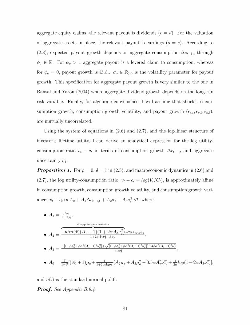
aggregate equity claims, the relevant payout is dividends (o = d). For the valuation

of aggregate assets in place, the relevant payout is earnings (o = e). According to

(2.8), expected payout growth depends on aggregate consumption ∆ct−1,t through

φo ∈ R. For φo > 1 aggregate payout is a levered claim to consumption, whereas

for φo = 0, payout growth is i.i.d.. σo ∈ R>0 is the volatility parameter for payout

growth. This specification for aggregate payout growth is very similar to the one in

Bansal and Yaron (2004) where aggregate dividend growth depends on the long-run

risk variable. Finally, for algebraic convenience, I will assume that shocks to con-

sumption growth, consumption growth volatility, and payout growth (εc,t, εσ,t, εo,t),

are mutually uncorrelated.

Using the system of equations in (2.6) and (2.7), and the log-linear structure of

investor’s lifetime utility, I can derive an analytical expression for the log utility-

consumption ratio vt − ct in terms of consumption growth ∆ct−1,t and aggregate

uncertainty σt.

Proposition 1: For ρ = 0, δ = 1 in (2.3), and macroeconomic dynamics in (2.6) and

(2.7), the log utility-consumption ratio, vt − ct = log(Vt/Ct), is approximately affine

in consumption growth, consumption growth volatility, and consumption growth vari-

ance: vt − ct ≈ A0 + A1∆ct−1,t + A2σt + A3σ2t ∀t, where

• A1 = βφc1−βφc ,

• A2 =

disappointment aversion︷ ︸︸ ︷−θβn(x)(A1 + 1)(1 + 2αA3ν

2σ) +2βA3µσφσ

1+2αA3ν2σ−βφσ

,

• A3 =−[1−βφ2

σ+βα2(A1+1)2ν2σ ]+√

[1−βφ2σ+βα2(A1+1)2ν2

σ ]2−4βα2(A1+1)2ν2σ

4αν2σ

,

• A0 = β1−β [(A1 +1)µc+ 1

1+2αA3ν2σ(A2µσ +A3µ

2σ−0.5αA2

2ν2σ)+ 1

2αlog(1+2αA3ν

2σ)],

and n(.) is the standard normal p.d.f..

Proof. See Appendix B.6.4

81

A1 is the consumption growth multiplier. The sign and magnitude of A1 depend

on consumption growth autocorrelation φc. If consumption growth is i.i.d. then A1

is zero. A3 is the multiplier for consumption growth variance σ2t . If the risk aversion

coefficient α is positive, then A3 is negative36. For A3 to be real, we require that the

terms inside the square root are positive, and that α is different than zero37. A2 is the

multiplier for consumption growth volatility σt, and captures first-order risk aversion

through the θn(x) term. For A3 negative and positive θ, then A2 is also negative. A0

is the constant term in the log utility-consumption ratio. For A0 to be well defined,

we require 1 + 2αA3ν2σ to be positive, and that α is non-zero. Finally, if consumption

growth is positively autocorrelated (φc > 0), and preference parameters (α, θ > 0) are

also positive, then the log utility-consumption ratio is procyclical since A1 is positive,

and A2, A3 are negative.

An immediate consequence of Proposition 1 is that we can express the disappoint-

ment aversion stochastic discount factor in (2.5) as a function of consumption growth

∆ct−1,t, and consumption growth volatility σt

Mt,t+1 ≈ elogβ−∆ct,t+1︸ ︷︷ ︸time correction

e−α{A0(1− 1

β)+[(A1+1)∆ct,t+1− 1

βA1∆ct−1,t]+A2(σt+1− 1

βσt)+A3(σ2

t+1−1βσ2t )}︸ ︷︷ ︸

second-order risk correction

× (2.9)

1 + θ 1{A0 + (A1 + 1)∆ct,t+1 + A2σt+1 + A3σ2t+1 <

1β(A0 + A1∆ct−1,t + A2σt + A3σ

2t )}

Et[1 + θ 1{A0 + (A1 + 1)∆ct,t+1 + A2σt+1 + A3σ2t+1 <

1β(A0 + A1∆ct−1,t + A2σt + A3σ2

t )}]︸ ︷︷ ︸disappointment correction

.

Mt,t+1 in (2.9) corrects expected future payoffs for timing, risk and disappointment,

much like the one in (2.5). The crucial difference between the two expressions is

that in equation (2.9) unobservable lifetime utility Vt+1 is expressed in terms of state

variables.

Armed with the expression for the stochastic discount factor, we can also solve

36Appendix B.6.4.37A detailed discussion on parameter restrictions can be found in Appendix B.6.4. The require-

ment α 6= 0, implies that preferences need to be non-separable across time.

82

for the one-period log risk-free rate (see Appendix B.6.5)

rf,t,t+1 ≈ −logβ + 1 · µc + 1 · φc∆ct−1,t︸ ︷︷ ︸impatience and future prospects

−0.5[2α(A1 + 1) + 1]σ2t︸ ︷︷ ︸

second-order risk aversion

− θn(x)σt.︸ ︷︷ ︸disappointment aversion︸ ︷︷ ︸

precautionary savings motive

(2.10)

Consumption growth terms(µc(1− φc), φc∆ct−1,t

)in (2.10) are multiplied by unity,

since the EIS is assumed equal to one, and thus consumption growth moves one-for-

one with interest rates. The last two terms in (2.10) reflect the precautionary motive

for investors to save. This motive depends on both risk and disappointment aversion.

Notice that second-order risk aversion terms depend on consumption growth variance

(σ2t ), while disappointment aversion terms depend on consumption growth volatility

(σt) due to the first-order risk aversion effect. For α, θ positive, higher uncertainty

(high values for σt and σ2t ) will force investors to save more in the risk-free technology,

and therefore decrease interest rates.

Turning now to risky financial assets, let Rm,t be the cum-payout, one-period,

gross return for a claim on a stream of aggregate payments (dividends or earnings).

If claims are traded in complete, frictionless markets, then the consumption-Euler

equation implies that

Et[Mt,t+1Rm,t,t+1

]= 1.

Using the results in Appendix B.4, aggregate log-returns rm,t,t+1 can be written as a

linear function of log price-payout ratios, and the Euler equation becomes

Et[Mt,t+1e

κm,0+κm,0zm,t+1−zm,t+∆om,t,t+1

]= 1,

where κm,0 and κm,1 are linearization constants, and zm,t = log Pm,tOm,t

is the log price-

payout ratio.

83

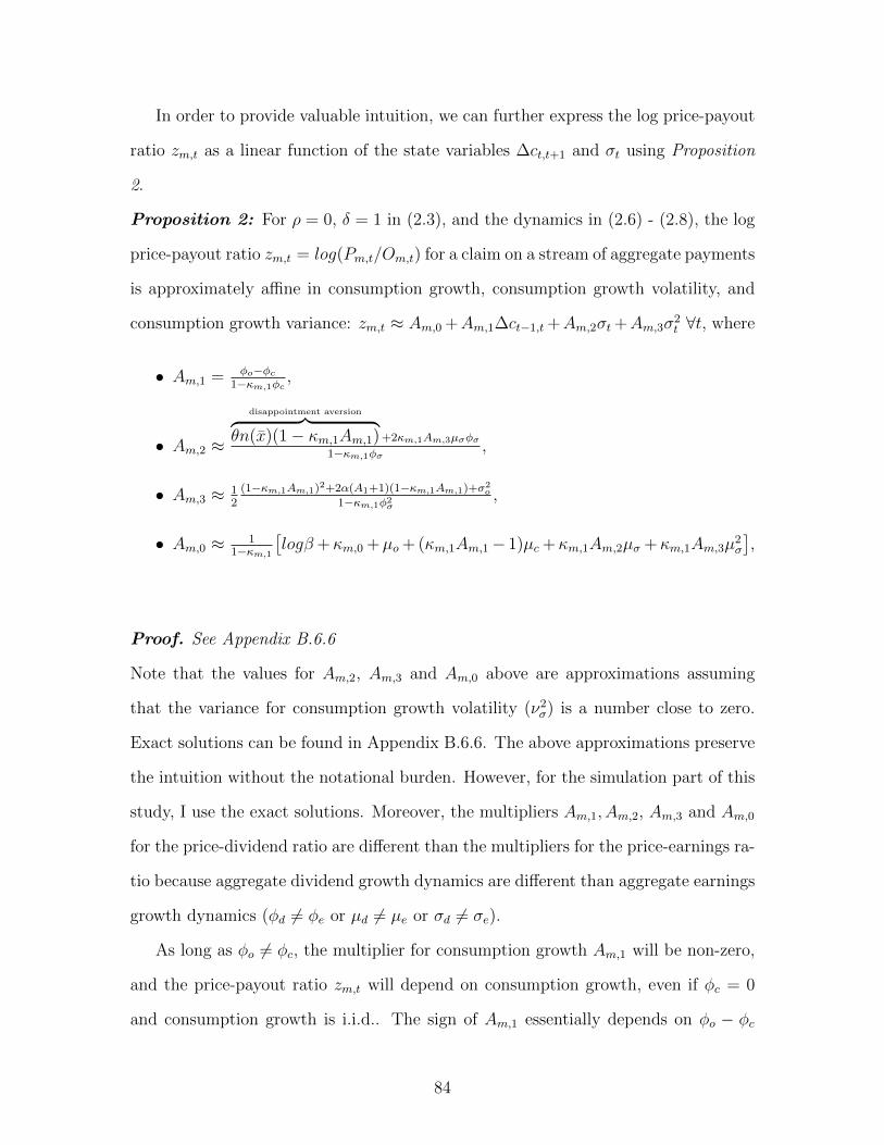
In order to provide valuable intuition, we can further express the log price-payout

ratio zm,t as a linear function of the state variables ∆ct,t+1 and σt using Proposition

2.

Proposition 2: For ρ = 0, δ = 1 in (2.3), and the dynamics in (2.6) - (2.8), the log

price-payout ratio zm,t = log(Pm,t/Om,t) for a claim on a stream of aggregate payments

is approximately affine in consumption growth, consumption growth volatility, and

consumption growth variance: zm,t ≈ Am,0 +Am,1∆ct−1,t +Am,2σt +Am,3σ2t ∀t, where

• Am,1 = φo−φc1−κm,1φc ,

• Am,2 ≈

disappointment aversion︷ ︸︸ ︷θn(x)(1− κm,1Am,1) +2κm,1Am,3µσφσ

1−κm,1φσ ,

• Am,3 ≈ 12

(1−κm,1Am,1)2+2α(A1+1)(1−κm,1Am,1)+σ2o

1−κm,1φ2σ

,

• Am,0 ≈ 11−κm,1

[logβ+κm,0 +µo + (κm,1Am,1− 1)µc +κm,1Am,2µσ +κm,1Am,3µ

2σ

],

Proof. See Appendix B.6.6

Note that the values for Am,2, Am,3 and Am,0 above are approximations assuming

that the variance for consumption growth volatility (ν2σ) is a number close to zero.

Exact solutions can be found in Appendix B.6.6. The above approximations preserve

the intuition without the notational burden. However, for the simulation part of this

study, I use the exact solutions. Moreover, the multipliers Am,1, Am,2, Am,3 and Am,0

for the price-dividend ratio are different than the multipliers for the price-earnings ra-

tio because aggregate dividend growth dynamics are different than aggregate earnings

growth dynamics (φd 6= φe or µd 6= µe or σd 6= σe).

As long as φo 6= φc, the multiplier for consumption growth Am,1 will be non-zero,

and the price-payout ratio zm,t will depend on consumption growth, even if φc = 0

and consumption growth is i.i.d.. The sign of Am,1 essentially depends on φo − φc

84

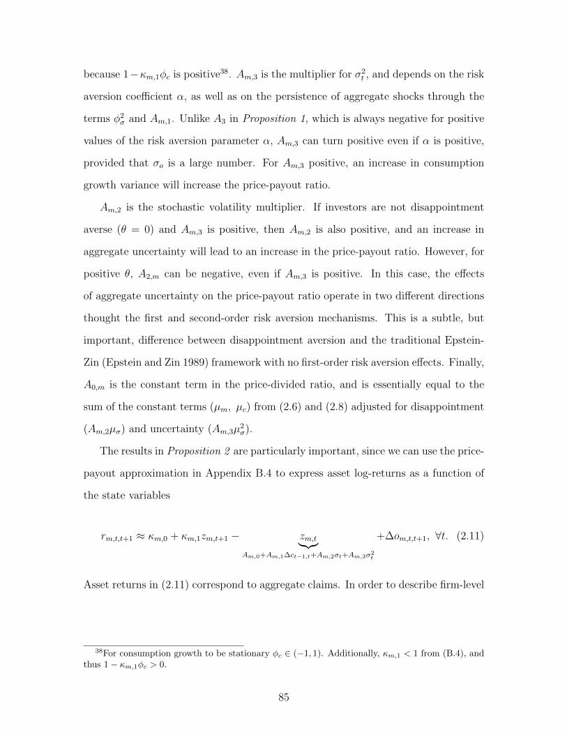
because 1−κm,1φc is positive38. Am,3 is the multiplier for σ2t , and depends on the risk

aversion coefficient α, as well as on the persistence of aggregate shocks through the

terms φ2σ and Am,1. Unlike A3 in Proposition 1, which is always negative for positive

values of the risk aversion parameter α, Am,3 can turn positive even if α is positive,

provided that σo is a large number. For Am,3 positive, an increase in consumption

growth variance will increase the price-payout ratio.

Am,2 is the stochastic volatility multiplier. If investors are not disappointment

averse (θ = 0) and Am,3 is positive, then Am,2 is also positive, and an increase in

aggregate uncertainty will lead to an increase in the price-payout ratio. However, for

positive θ, A2,m can be negative, even if Am,3 is positive. In this case, the effects

of aggregate uncertainty on the price-payout ratio operate in two different directions

thought the first and second-order risk aversion mechanisms. This is a subtle, but

important, difference between disappointment aversion and the traditional Epstein-

Zin (Epstein and Zin 1989) framework with no first-order risk aversion effects. Finally,

A0,m is the constant term in the price-divided ratio, and is essentially equal to the

sum of the constant terms (µm, µc) from (2.6) and (2.8) adjusted for disappointment

(Am,2µσ) and uncertainty (Am,3µ2σ).

The results in Proposition 2 are particularly important, since we can use the price-

payout approximation in Appendix B.4 to express asset log-returns as a function of

the state variables

rm,t,t+1 ≈ κm,0 + κm,1zm,t+1 − zm,t︸︷︷︸Am,0+Am,1∆ct−1,t+Am,2σt+Am,3σ2

t

+∆om,t,t+1, ∀t. (2.11)

Asset returns in (2.11) correspond to aggregate claims. In order to describe firm-level

38For consumption growth to be stationary φc ∈ (−1, 1). Additionally, κm,1 < 1 from (B.4), andthus 1− κm,1φc > 0.

85

asset returns, we need to introduce idiosyncratic shocks as follows

ri,t,t+1 ≈ κm,0 + κm,1zm,t+1 − zm,t + ∆om,t,t+1︸ ︷︷ ︸systematic component

+ σiεi,t+1︸ ︷︷ ︸idiosyncratic part

, (2.12)

for cum-payout returns, and

rxi,t,t+1 = zm,t+1 − zm,t + ∆om,t,t+1 + σiεi,t+1, (2.13)

for ex-payout returns. εi,t+1 are i.i.d. N(0,1) idiosyncratic shocks, orthogonal to the

rest of the aggregate shocks in (2.6)-(2.8). The above specification for firm-level

returns matches perfectly a long-standing concept in finance according to which asset

returns can be decomposed into a systematic part, and an idiosyncratic one. Note

that for equity returns the relevant payout in (2.11) - (2.13) is dividends (o = d),

whereas for assets in place returns the relevant payout is earnings (o = e).

2.5 Simulation results for the disappointment aversion dis-

count factor

2.5.1 Preference parameters, and state variable moments for the simu-

lated economy

The EIS and the GDA parameters for the disappointment aversion discount fac-

tor in (1.3) are assumed equal to one for analytical tractability. For the remaining

parameters, I set the risk aversion coefficient α equal to 1.8 and the disappointment

aversion parameter θ equal to 2.030. These values are within the range of clinical

estimates39, and are very similar to those used in Bonomo et al. (2011). The value

for θ implies that whenever lifetime utility is below its certainty equivalent (disap-

pointment events), investors penalize losses 3 times more than during normal times.

39Gill and Prowse (2012).

86

Finally, the rate of time preference β is equal to 0.9955. In the deterministic steady-

state of the economy, an additional $1 of consumption tomorrow is worth $0.9955

today.

In order to explain the market-wide equity premium, Routledge and Zin (2010)

employ a constant consumption growth variance framework, and set θ equal to 9 with

α equal to -1 (second-order risk neutrality). In Bonomo et al. (2011) consumption

growth variance is stochastic, θ is 2.33, and α is 1.5. Choi et al. (2007) conduct clinical

experiments on portfolio choice under uncertainty, and find disappointment aversion

coefficients that range from 0 to 1.876, with a mean of 0.39. They also estimate

second-order risk aversion parameters that range from -0.952 to 2.871, with a mean

of 1.448. Using experimental data on real effort provision, Gill and Prowse (2012)

estimate disappointment aversion coefficients ranging from 1.260 to 2.070. Ostrov-

naya et al. (2006) estimate disappointment aversion parameters from stock market

data using market wide stock market returns as the explanatory variable, instead

of consumption growth. Their estimates for θ range from 1.825 to 2.783. Finally,

Delikouras (2013) assumes constant consumption growth volatility, and provides θ

estimates around 4.6, and risk aversion estimates that range from 10 up to 16.

Table 2.8.3 summarizes parameter values for state variable dynamics in (2.6)-(2.8).

These values are carefully chosen so that simulated moments match those observed

in real data. Many of these parameters have been used in previous studies. For

instance, the consumption growth multipliers φd and φe in (2.8) are equal to 3 as

in Bansal and Yaron (2004). Earnings are considered a levered claim to consump-

tion (φe > 1) because the endowment model ignores other claims to earnings such

as salaries, depreciation, and taxes that need to be paid out before interest and div-

idends40. Volatility parameters for dividends and earnings growth (σd = 7.1664 and

40Also, for uncorrelated macroeconomic shocks in (2.6)-(2.8), letting φe (φd) be larger than one isthe only way to obtain plausible correlations between earnings (dividend) growth and consumptiongrowth. Chen et al. (2009), p. 3404, set φd equal to 3.5 and φe equal to 2.7.

87

σe = 2.2011) are larger than one, because dividend and earnings growth are much

more volatile than consumption growth. The autocorrelation parameter for aggre-

gate consumption growth volatility is 0.971 because, according to previous results41,

aggregate uncertainty is a very persistent process. Finally, idiosyncratic volatility σi

is set equal to 0.210 so as to match the Sharpe ratio for the median Baa firm which

is 0.220 (Chen et al. 2009, p. 3377).

Despite the similarities with previous studies, there are a few notable exceptions.

First, in Bansal and Yaron (2004) and Bansal et al. (2007), expected consumption

growth is a very persistent process, whereas in Chen et al. (2009) and Bonomo et al.

(2011) consumption growth is i.i.d. (φc=0). Here, I set the autocorelation parameter

φc equal to 0.5 to match the persistence in BEA consumption data. Second, the

volatility parameter µσ in Bansal and Yaron (2004) and Bonomo et al. (2011) is

quite high. Their values for µσ imply that annual consumption growth volatility is

approximately 3%, which is more than two times the volatility observed in the BEA

sample (1.3% from Table 2.8.4). In this study, µσ is equal to a very small value

(0.0004) so that consumption growth volatility remains low. Finally, the linearization

constant zm for log price-payout ratios in (B.4) is equal to 3, which is very close to

the unconditional mean for the stock market log price-dividend ratio (Table 2.8.6).

Table 2.8.4 shows simulated and sample moments for all macroeconomic variables.

Simulated values for the state variables are according to the system in (2.6)-(2.8),

using parameter values from Table 2.8.342. Simulated moments for aggregate con-

sumption growth are very close to actual ones (mean 1.834% vs. 1.838% in the data,

autocorrelation 0.504 vs. 0.502), with the exception of consumption growth volatil-

ity which is higher for the simulated economy (1.914% vs. 1.346% in the data)43.

41Bansal and Yaron (2004), Bansal et al. (2007), Lettau et al. (2007), Chen et al. (2009), andBonomo et al. (2011).

42Because (2.7) admits negative volatility, if at some point volatility becomes negative, then thenegative observation is replaced with the previous observation.

43In Chen et al. (2009) consumption growth volatility is around 1.5%. In Bansal and Yaron(2004) and Bonomo et al. (2011) consumption growth volatility is 3%, whereas consumption growth

88

Simulated moments for aggregate dividend growth are very realistic as well (mean

1.796% vs. 2.107%, volatility 13.232% vs. 13.079% in the data). However, the au-

tocorrelation for the simulated aggregate dividend growth process is positive (0.093),

whereas dividend growth in the data is a mean reverting process (-0.278). Finally,

the simulated dividend growth and consumption growth processes are positively au-

tocorrelated much like in the 1946-2011 sample (0.218 vs. 0.286 in real data44).

Expected earnings growth for the simulated economy is positive (1.819%), and

similar to the to expected value for consumption and dividend growth. Even though,

in the long-run, expected growth rates should be almost identical because dividends

and earnings are cointegrated, Belo et al. (2012) explain how endogenous capital de-

cisions can make dividends riskier than earnings in the short-run. Expected earnings

growth in the sample is negative (-3.831%), and approximately equal to expected infla-

tion, because CRSP-Compustat nominal earnings have been exponentially detrended

due to the increasing number of firms in the Compustat sample over time. Earnings

growth volatility is lower than in the 1946-2011 sample (6.784% vs. 7.057%). Simi-

larly, the simulated correlation coefficient between earnings growth and consumption

growth is lower than the sample one (0.425 vs. 0.487)45. Macroeconomic uncer-

tainty is hard to measure, and, therefore, there aren’t any readily available data to

benchmark simulation results for σt. Nevertheless, parameter values for uncertainty

dynamics in (2.8) are based on previous results commonly used in the asset pricing

literature46.

volatility in Shiller’s data is 1.8%.44For their habit model, Chen et al. (2009), p. 3377, assume that the correlation coefficient

between aggregate dividends and aggregate consumption growth is equal to 0.60, more than twicethe estimated value 0.286 in Table 2.8.4.

45The correlation coefficient between consumption growth and earnings growth in Chen et al.(2009) is 0.48 (p. 3377).

46Bansal and Yaron (2004), Bansal et al. (2007), Chen et al. (2009), and Bonomo et al. (2011).

89

2.5.2 Simulation results for Baa-Aaa credit spreads

The main pricing equation used in this study is the consumption-Euler equation

for zero-coupon, corporate bonds that are subject to default at the expiration date

E[yi,t,t+T ] = E[− 1

TlogEt

[( T∏j=1

Mt+j−1,t+j

)(1− Lt+T1{rxi,t,t+T < Di,t+T}

)]], (2.14)

in which Mt,t+j is the disappointment aversion stochastic discount factor from (2.9),

Lt+T are losses given default, rxi,t,t+T are ex-payout, log-returns for assets in place (not

equity returns) according to (2.13), and Di,t+T is the default boundary. Although

bond yields in Table 2.8.1 are measured in nominal terms, the model economy has

been simulated in real terms, and thus, model implied spreads are inflation-free. To

the extend that inflation risk premia are approximately equal for Baa and Aaa bonds,

then nominal Baa-Aaa credit spreads should be very similar to real Baa-Aaa credit

spreads. Unlike the model in (2.1), losses given default Lt+T and default boundaries

Di,t+T are allowed to vary over time, and also be functions of the state variables

1− Lt+T = arec,0 + arec,c∆ct+T−1,t+T , (2.15)

Di,t+T = ai,def,0 + adef,c(∆ct+T−1,t+T −

µc1− φc

)+ adef,σ

(σt+T −

µσ1− φσ

). (2.16)

Table 2.8.5 shows the main empirical results in this study which have been ob-

tained through the simulation process discussed in Appendix B.5. Panel A in Table

2.8.5 specifies values for the Baa and Aaa default boundaries which are expressed in

terms of asset log-returns. For example, the 4yr constant Baa default boundary is

equal to -0.998 which means that the value of assets in place needs to decrease to

e−0.998 = 36.861% of initial value before a Baa firm defaults47.

Simulated default probabilities in Panel B are practically indistinguishable from

47Chen et al. 2009 also assume a similar constant default boundary for 4 year Baa bonds (p.3384).

90

default rates in the Moody’s report due to appropriately selecting default boundaries.

The default rates in Panel B guarantee that the stochastic discount factor in (2.9)

generates plausible credit spreads because investors severely penalize default states

through the disappointment aversion mechanism, and not because default probabili-

ties are abnormally high. Finally, Panel C in Table 2.8.5 shows average credit spreads

implied by the disappointment aversion discount factor in (2.9) with preference pa-

rameters from Table 2.8.3, and aggregate state variable dynamics according to the

system in (2.6)-(2.8). In order to address the shortcomings of the benchmark model in

(2.1), I consider four different cases: I) constant recovery rates and default boundaries,

II) procyclical recovery rates according to (2.15) and constant default boundaries, III)

constant recovery rates and countercyclical default boundaries according to (2.16),

and IV) procyclical recovery rates and countercyclical default boundaries.

Expected credit spreads for the disappointment aversion discount factor in case I

are larger than those for the benchmark model (average increase across maturities 15

bps) because disappointment averse investors heavily penalize periods during which

lifetime utility is less than its certainty equivalent (disappointment events). During

these periods, Baa defaults happen more often than defaults for Aaa firms, which are

fairly acyclical. In other words, Baa corporate bonds expose the aggregate investor

to more disappointment risk than Aaa bonds. Therefore, in order for Baa bonds to

be part of the aggregate portfolio, these claims should be discounted at higher rates

than Aaa bonds.

Relative to the benchmark model in (2.1), case I in Panel C is different in two very

important ways. First, as explained by Lemma 1 in Appendix B.6.1, the benchmark

model implicitly assumes CRRA preferences. Although concave CRRA utility func-

tions overweigh unfavorable outcomes, they do not capture asymmetries in marginal

utility, because CRRA preferences are isoelasic. On the other hand, the disappoint-

ment model relies heavily on investors penalizing losses that happen during periods

91

when lifetime utility is below the certainty equivalent 1+θ times more than loses dur-

ing normal times. Second, disappointment aversion preference induce time-variation

in risk attitudes. This time-variation is further amplified by stochastic consump-

tion growth volatility in (2.7) to generate substantially time-variation in expected

returns and Sharpe ratios. Recent results in asset pricing suggest that time-variation

in Sharpe ratios is almost a necessary condition for resolving a number of prominent

asset pricing puzzles48, including the credit spread puzzle.

Nevertheless, disappointment aversion alone cannot fully rationalize expected Baa-

Aaa credit spreads, especially for very short maturities, since, according to Table

2.8.5, 41 bps in expected credit spreads for 4yr bonds remain unexplained by the

disappointment model. These results should not cast any doubt on the explanatory

power of disappointment aversion. According to Chen et al. (2009), neither the

habit, nor the long-run risk models can explain credit spreads49, unless we assume

time-varying recovery rates or stochastic default boundaries.

Table 2.8.2 provides evidence that recovery rates are procyclical. The assumption

of constant recovery rates therefore ignores an important risk source for credit spreads.

Case II in Table 2.8.5 relaxes this assumption, and, based on the results of Table 2.8.2,

assumes that losses given default Lt+T are a linear function of aggregate consumption

growth as in (2.15) in which arec,c is set equal to 4.464 from Table 2.8.2. The addition

of procyclical recovery rates increases Baa-Aaa spreads implied by the disappointment

model by 34 bps on average across maturities relatively to the benchmark model in

(2.1), and by 23 bps relatively to the benchmark model with procyclical recovery

rates in (2.2).

In the case of countercyclical losses given default, corporate bonds need to com-

pensate the disappointment averse investor for two sources of systematic risk. The

48Campbell and Cochrane (1999), Bansal and Yaron (2004), Verdelhan (2010), Routledge andZin (2010), Bansal and Shaliastovich (2013).

49Chen et al. (2009) p. 3384 and p. 3405.

92

first one is related to the fact that during economic downturns default frequencies for

Baa firms increase more than default frequencies for Aaa bonds. The second source of

systematic risk captures the fact that during disappointment periods recovery rates

decrease. Moreover, disappointment aversion preferences punish the procyclicality

of recovery rates more severely than power utility which is implicitly assumed by

the model in (2.2). The first-order risk aversion mechanism amplifies recovery rate

risk, despite the relatively low covariance between recovery rates and consumption

growth. However, despite the improvement relatively to the benchmark case in (2.2),

even with countercyclical recovery rates, 26 bps in 4yr expected credit spreads (17

bps for 10yr maturities) cannot be explained by case II of the disappointment model.

Cases III and IV in Table 2.8.5 assume stochastic default boundaries. Since these

boundaries are hard to measure, parameters for the stochastic default boundary have

been calibrated so that default rates for the simulated economy match actual ones.

Unlike Chen (2010) or Bhamra et al. (2010), but similar to Chen et al. (2009),

default boundaries in this study are exogenous, even though they are functions of state

variables. The calibrated values for the default boundary functions in (2.16) imply

that these boundaries are strongly countercyclical, since they co-move negatively with

consumption growth, and positively with macroeconomic uncertainty. In bad times,

when consumption growth (volatility) is lower (higher) than its unconditional mean,

default boundaries are low in absolute value, and thus managers find it easier to

declare bankruptcy. In good times, when consumption growth (volatility) is higher

(lower) than its mean, default boundaries are high in absolute value, and firms do

not default as easily as in bad times.

Countercyclical default boundaries lead to a larger number of defaults during

economic downturns, and fewer number of defaults during good times, yet, uncondi-

tionally, average default rates are equal to the ones observed in actual data. Coun-

tercyclical default boundaries essentially imply that default events covary more with

93

aggregate macroeconomic conditions relative to cases I and II. The combination of dis-

appointment aversion preferences with countercyclical default boundaries (case III)

improves the fit of the baseline disappointment model (case I), and also increases

model implied expected credit spreads by 25 bps across maturities relative to the

benchmark model in (2.1). Nevertheless, the increase in credit spreads induced by

stochastic default boundaries in case III is less than the increase due to procyclical

recovery rates in case II, and leaves 29 bps in 4yr expected credit spreads (25 bps in

10yr bonds) unexplained.

Finally, the disappointment model with procyclical recovery rates and counter-

cyclical boundaries (case IV) can fit average credit spreads for short (100 bps vs. 103

bps for 4yr spreads) and medium maturities (129 bps vs. 131 bps for 10yr spreads),

but severely overestimates credit spreads at the long end of the term structure (148

bps vs. 112 bps for 15yr bonds). Countercyclical default boundaries increase the fre-

quency of defaults during bad times, while procyclical recovery rates increase losses

given default during periods of low economic growth. Because periods of high Baa

default rates and high losses given default are also associated with disappointment

events (lifetime utility below its certainty equivalent), disappointment averse investors

require larger compensation for holding Baa bonds than Aaa bonds.

Overall, results in Table 2.8.5 suggest that as long as we allow for procyclical

recovery rates and countercyclical default boundaries, disappointment aversion pref-

erences are able to resolve the credit spread puzzle using risk and disappointment

aversion parameters that are consistent with recent experimental results. However,

as shown in Figure 2.9.4, by fitting mean credit spreads for short and medium ma-

turities, the disappointment model overestimates mean credit spreads for maturities

longer than 15 years. The credit spread literature mostly considers 4yr or 10yr bonds,

and does not provide any results on long maturities. Therefore, we cannot assess the

relative performance of the disappointment aversion model for long maturities. More-

94

over, matching average credit spreads for very short maturities (1-3yr) still remains

an open question50.

Although, the goal of this paper is not a horse race between prominent asset

pricing models, we need to highlight that the disappointment aversion mechanism

is unique. First, disappointment aversion preferences fully encompass recent clinical

and field evidence for behavior under uncertainty which emphasize the importance of

expectation-based reference-dependent utility51. The key mechanism in disappoint-

ment aversion is asymmetric marginal utility over gains and losses. Gains and losses

are, in turn, endogenously characterized by the forward-looking certainty equivalent

for lifetime utility.

Asymmetric marginal utility is not present in the habit model, which assumes

a backwards-looking unobservable habit process, and, according to Ljungqvist and

Uhlig (2009), leads to policy inconsistencies for the central planner. Furthermore, in

the habit model of Campbell and Cochrane (1999) consumption never drops below its

habit, otherwise marginal utility becomes infinity. On the other hand, for disappoint-

ment aversion preferences it is precisely periods during which consumption growth

falls below its certainty equivalent that are important for credit spreads. Asymmetric

marginal utility is not captured by the long-run risk model either which assumes a

highly persistent mean in expected consumption growth52.

2.5.3 Equity premium, and the risk-free rate

By assuming extremely high risk premia, one could possibly improve the perfor-

mance of consumption-based models in fitting credit spreads. However, high risk

premia would also imply abnormally high expected returns for the stock market.

50According to Table 2.8.1, default rates for for 1 up to 3 years are almost zero. Because no assetpricing model can map zero default rates for short term bonds into measurable yields, the creditspread literature focuses on medium to long term maturities (4-10yr).

51Choi et al. (2007), Post et al. (2008), Doran (2010), Crawford and Meng (2011), Abeler et al.(2011), Gill and Prowse (2012).

52Beeler and Campbell (2012), Bonomo et al. (2011).

95

In this section, I show that the disappointment aversion model in (2.9) can match

moments for the equity premium, the price-dividend ratio, and the risk-free rate rea-

sonably well, with the same preference parameters and state variable dynamics from

Table 2.8.3. Equity returns, the risk-free rate, and the price-dividend ratio, have been

simulated according to the expressions in (2.11), (2.10), and Proposition 2 respec-

tively, while sample moments are calculated using the data described in subsection

2.3.1.

According to Table 2.8.6, simulated stock market returns for the disappoint-

ment aversion model have a high mean (6.653% vs. 6.581% in the data), are quite

volatile (15.049% vs. 17.216% in the data) and i.i.d.(ρ(rm,t,t+1, rm,t−1,t) = 0.035

vs. -0.030 in the data), and are positively correlated with consumption growth(

ρ(rm,t,t+1,∆ct−1,t) = 0.463 vs. 0.503 in the data). The disappointment model also

predicts a highly autocorrelated (0.650 vs. 0.696 in the data) and low mean (0.962%

vs. 0.928% in the data) risk-free rate, yet the variance for the simulated risk-free rate

is substantially smaller than the sample estimate (1.163% vs. 2.727%). Finally, even

though results for the price-dividend ratio are fairly accurate, especially in terms of

persistence (0.891 vs. 0.950 in the data), the simulated price-dividend in the dis-

appointment averse economy has lower mean (3.000 vs. 3.433), and is less volatile

(0.227 vs. 0.467) than the one obtained from the CRSP database.

Traditional consumption-based asset pricing models with time-separable power

utility need exorbitant values for the risk aversion coefficient, around 50 for annual

data53, and around 150 for quarterly data54, in order to match expected stock market

returns. Further, extremely large risk aversion parameters lead to very volatile risk-

free rates55. Non-separable Epstein-Zin preferences without first-order risk aversion

53Mehra and Prescott (1985), Cochrane (2001), Yogo (2004), Liu et al. (2009), Routldege andZin (2010), Delikouras (2013).

54Aıt-Sahalia et al. (2004), Yogo (2004), Delikouras (2013).55Weil (1989), Delikouras (2013).

96

effects, also require large coefficients of risk aversion, around 3056 to match expected

stock market returns, unless we assume a very persistent process for expected con-

sumption growth57. These empirical discrepancies are ingeniously concealed by the

benchmark models in (2.1) and (2.2) or any other model that directly uses risk-

neutral pricing because these models do not explicitly model investor preferences. In

contrast, the disappointment aversion discount factor in (2.9) can generate realistic

asset pricing moments using parameter values that are consistent with clinical results

for behavior under uncertainty.

2.5.4 Comparative results for alternative preference parameters

The main goal of the paper is to examine whether disappointment aversion pref-

erences can explain asset prices across different financial markets with risk and dis-

appointment aversion parameters calibrated to experimental findings. This section

performs a sensitivity analysis on preference parameters for the disappointment aver-

sion discount factor in (2.9). Comparative results focus on the two parameters that

affect risky choices, the risk and disappointment aversion parameters α and θ, while

the rest of the parameters in Table 2.8.3 as well as model dynamics from (2.6)-(2.8)

are kept constant.

The choice of alternative parameter values for the disappointment aversion model

serves three purposes. First, alternative parameters need to be close to clinical esti-

mates. Second, alternative parameter values should be able to identify the marginal

importance of the first and second-order risk aversion channels. Finally, the choice

of these alternative values ought to guarantee that the multipliers A0 − A3, and

Am,0−Am,3 are well defined and real. The systems of equations in Proposition 1 and

Proposition 2 impose constraints on the magnitude of the risk aversion parameter.

For instance, if α is greater than 8.7, then the solutions to the quadratic equations for

56Routldege and Zin (2010), Delikouras (2013).57Bonomo et al. (2011), Beeler and Campbell (2012), Delikouras (2013)

97

A3 and Am,3 are imaginary numbers, unless we specify different parameters for the

state variable dynamics in (2.6)-(2.8). In contrast, there are no constraints imposed

on θ, because A2 and Am,2 are solutions to linear equations.

For the first alternative scenario, the risk aversion parameter is set equal to -1

(second-order risk neutrality), and the disappointment aversion parameter is equal

to 3. By setting α equal to -1, we are essentially downgrading the importance of

consumption growth variance σ2t as a state variable. This is done through the param-

eters A3 and Am,3 which significantly decrease in magnitude, and even turn positive

due to second order risk neutrality. For the baseline disappointment model in Table

2.8.5 and Table 2.8.6 where α is positive, A3 and Am,3 are large in absolute value and

negative.

According to Table 2.8.7, if we turn off the risk aversion channel, and increase the

magnitude for the disappointment aversion parameter, then the expected risk-free

rate decreases relative to the baseline scenario (0.519% vs. 0.962%) because the first-

order precautionary savings motive intensifies. In contrast, expected equity premia

remain essentially the same relative to the baseline disappointment model (5.676% vs.

5.691% for the baseline model). Even though the reduction in expected excess stock

returns is almost zero, the decrease in expected credit spreads relative to the baseline

scenario in Table 2.8.7 is quite impressive, approximately -29 bps for 4yr maturities

across all four cases. Results in Table 2.8.7 suggest that although equity premia

are insensitive to the second-order risk aversion channel, credit-spreads are hugely

affected by setting α equal to -1. Because Baa defaults are very rare events, even the

slightest change in systematic risk can lead to substantial changes in credit spreads.

On the other hand, equity premia are not sensitive to second-order risk-neutrality

because stock market returns are not related to rare events.

For the second alternative scenario, the disappointment aversion channel is turned

off (θ = 0), and the risk aversion parameter is set equal to 5. Although 5 is a reason-

98

able value in the asset pricing literature, experimental results imply that α cannot be

greater than 2.858. In the absence of the first-order risk aversion mechanism, there

is an important decrease in average credit spreads relative to the baseline calibration

for the disappointment model, approximately -38 bps for 4yr maturities across all

four cases. Furthermore, expected excess stock returns are almost zero, while the

expected risk-free rate doubles in magnitude (2.000%), because, without disappoint-

ment aversion, the precautionary savings motive attenuates. Table 2.8.7 highlights

the importance of both first- and second-order risk aversion terms in generating mea-

surable credit spreads. Asset pricing models that do not include disappointment

aversion preferences, usually substitute first-order risk aversion effects with highly

persistent shocks to the stochastic discount factor through the habit or the long-run

risk mechanisms59.

2.6 Related literature

Before concluding the discussion on the credit spread puzzle, I will briefly relate

the disappointment framework to some key results in the corporate bond literature.

Merton (1974) was one of the first authors to propose a unified framework for the

valuation of corporate securities, bonds and equities, which are priced as contingent

claims written on a firm’s assets in place. Previous results on the inability of the

Merton model to match credit spreads date back to Jones et al. (1984), while Huang

and Huang (2012) show that the credit puzzle is robust to a variety of specifications

for the risk-neutral dynamics of asset returns.

In Merton’s early framework, there were no taxes, no bankruptcy costs, and capital

structure choices were irrelevant. Leland (1994) and Leland and Toft (1996), extend

Merton’s framework to account for tax benefits of debt, bankruptcy costs, and optimal

58Choi et al. (2007).59Campbell and Conchrane (1999), Bansal and Yaron (2004).

99

leverage decisions. Goldstein et al. (2001) also propose an asset pricing model for

corporate bonds in which the government, bondholders, and equityholders all have

stakes in the firm’s EBIT-generating process. In the Goldstein et al. model, bond

coupons, default, and leverage are all endogenous decisions. However, all these papers

rely directly on risk-neutral dynamics, remain silent on investor preferences, and do

not really focus on the empirical performance of these models across financial markets.

Bhamra et al. (2010) also propose a unified framework to explain the equity

premium and the credit-spread puzzle. Even though they use risk-neutral dynamics,

and do not focus on investor preferences either60, they provide a comprehensive model

with endogenous capital structure and default decisions in order to resolve the equity

premium and credit spread puzzles. Nevertheless, their model generates a credit

spread of only 45 bps for 5yr maturities (75 bps for 10yr maturities, p. 670), and an

equity risk premium of 3.19%.

Chen et al. (2009) compare the habit model of Campbell and Cochrane (1999),

and the long-run risk model of Bansal and Yaron (2004) for their ability to explain

the credit spread puzzle while generating possible moments for the stock market.

Although, both models can resolve the equity premium puzzle, the long-run risk model

has difficulties in generating measurable credit-spreads, while the habit-model needs

to be combined with countercyclical default boundaries or procyclical recovery rates

in order to fit Baa-Aaa credit spreads. Finally, Chen (2010) provides a parsimonious

general equilibrium model in order to resolve the credit spread and underleverage

puzzles, while matching moments for equity risk premia. However, he focuses only

on 10yr maturities, while he sets the risk aversion coefficient equal to 6.5, and the

EIS equal to 1.5., even though a number of empirical results suggest that61 the EIS

cannot be larger than one.

Table 2.8.8 shows model implied credit spreads and expected equity premia calcu-

60Although they assume Epstein-Zin utility for the aggregate investor.61Hall (1988), Bonomo et al. (2011), and Beeler and Campbell (2012).

100

lated in previous works. Notice that almost all results focus on 4yr or 10yr maturities

and remain silent on longer maturities. Furthermore, this paper is the first to im-

pose a stochastic discount factor which is microfounded on experimental evidence for

behavior under risk.

2.7 Conclusion

The aim of this paper is to examine whether disappointment aversion preferences

can help us resolve the credit spread puzzle within a consumption-based asset pric-

ing framework of an endowment economy. Given the relative success of first-order

risk aversion preferences in explaining other stylized facts in financial markets, the

disappointment aversion discount factor seems a natural candidate for correctly pric-

ing corporate bonds. However, the first-order risk aversion mechanism implied by

disappointment aversion is not powerful enough to map low probabilities of default

into measurable Baa-Aaa credit spreads. Only when the disappointment model is

combined with countercyclical losses given default and default boundaries, can dis-

appointment aversion preferences resolve the credit spread puzzle. This is in line

with the conclusions in Chen et al. (2009), according to which neither the habit nor

the long-run risk models can price Baa corporate bonds, unless we assume additional

sources of risk such as procyclical recovery rates, countercyclical default boundaries

or stochastic idiosyncratic volatility.

Furthermore, by fitting credit spreads for the short and medium term, the disap-

pointment model tends to overestimate credit spreads for long maturities (15yr+).

Traditional consumption-based asset pricing models (habit, long-run risk) have only

been tested against 4yr or 10yr bond maturities. It would be interesting to examine

the predictions of these models for longer maturities, as well as for the ultra short run.

Another direction for future research is to introduce disappointment aversion prefer-

ences in a world where capital structure choices matter so as to endogenize default

101

decisions. In spite of all these issues, the disappointment model is quite successful

in explaining not just corporate bond prices, but also key moments for stock market

returns, the risk-free rate, and the price-dividend ratio using preference parameters

that are consistent with experimental data for choices under uncertainty.

102

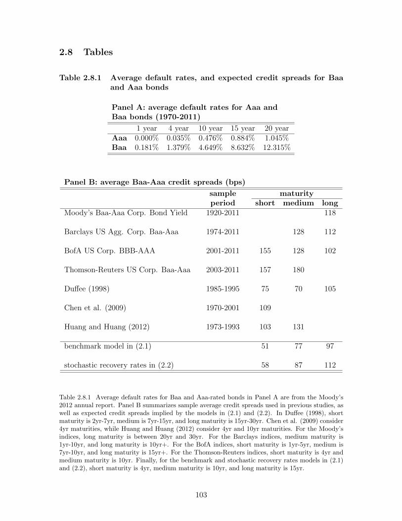
2.8 Tables

Table 2.8.1 Average default rates, and expected credit spreads for Baaand Aaa bonds

Panel A: average default rates for Aaa andBaa bonds (1970-2011)

1 year 4 year 10 year 15 year 20 yearAaa 0.000% 0.035% 0.476% 0.884% 1.045%Baa 0.181% 1.379% 4.649% 8.632% 12.315%

Panel B: average Baa-Aaa credit spreads (bps)

sample maturityperiod short medium long

Moody’s Baa-Aaa Corp. Bond Yield 1920-2011 118

Barclays US Agg. Corp. Baa-Aaa 1974-2011 128 112

BofA US Corp. BBB-AAA 2001-2011 155 128 102

Thomson-Reuters US Corp. Baa-Aaa 2003-2011 157 180

Duffee (1998) 1985-1995 75 70 105

Chen et al. (2009) 1970-2001 109

Huang and Huang (2012) 1973-1993 103 131

benchmark model in (2.1) 51 77 97

stochastic recovery rates in (2.2) 58 87 112

Table 2.8.1 Average default rates for Baa and Aaa-rated bonds in Panel A are from the Moody’s2012 annual report. Panel B summarizes sample average credit spreads used in previous studies, aswell as expected credit spreads implied by the models in (2.1) and (2.2). In Duffee (1998), shortmaturity is 2yr-7yr, medium is 7yr-15yr, and long maturity is 15yr-30yr. Chen et al. (2009) consider4yr maturities, while Huang and Huang (2012) consider 4yr and 10yr maturities. For the Moody’sindices, long maturity is between 20yr and 30yr. For the Barclays indices, medium maturity is1yr-10yr, and long maturity is 10yr+. For the BofA indices, short maturity is 1yr-5yr, medium is7yr-10yr, and long maturity is 15yr+. For the Thomson-Reuters indices, short maturity is 4yr andmedium maturity is 10yr. Finally, for the benchmark and stochastic recovery rates models in (2.1)and (2.2), short maturity is 4yr, medium maturity is 10yr, and long maturity is 15yr.

103

Table 2.8.2 OLS regression of recovery rates on aggregate consumptiongrowth (1982-2011)

arec,c 4.461(3.036)

R2 24.767%

Table 2.8.2 shows results for the OLS regression of recovery rates on contemporaneous consumptiongrowth. Recovery rates for senior subordinate debt are from the Moody’s 2012 report. arec,c is theOLS estimate with the t-statistic in parenthesis.

104

Table 2.8.3 Preference parameters, and state variable dynamics for thebaseline disappointment model

variable variable description variable valueEIS elasticity of intetemporal substitution 1δ generalized disappointment aversion 1β rate of time preference 0.9955α risk aversion 1.8000θ disappointment aversion 2.0303

µc consumption growth constant 0.0091φc consumption growth autocorrelation 0.5026

µσ volatility constant 0.0004φσ volatility autocorrelation 0.9715νσ volatility of volatility 0.0017

µd dividend growth constant -0.0367φd leverage parameter for dividend growth 3σd volatility parameter for dividend growth 7.1664

µe earnings growth constant -0.0367φe leverage parameter for earnings growth 3σe volatility parameter for earnings growth 2.2011

σi idiosyncratic return volatility 0.2100

zm linearization constant for the price-payout ratio in (B.4) 3x linearization constant for the normal c.d.f. in (B.9) 0

Table 2.8.3 summarizes preference parameters for the disappointment aversion stochastic discountfactor in (2.9), as well as model parameters for aggregate state dynamics in equations (2.6)-(2.8).

105

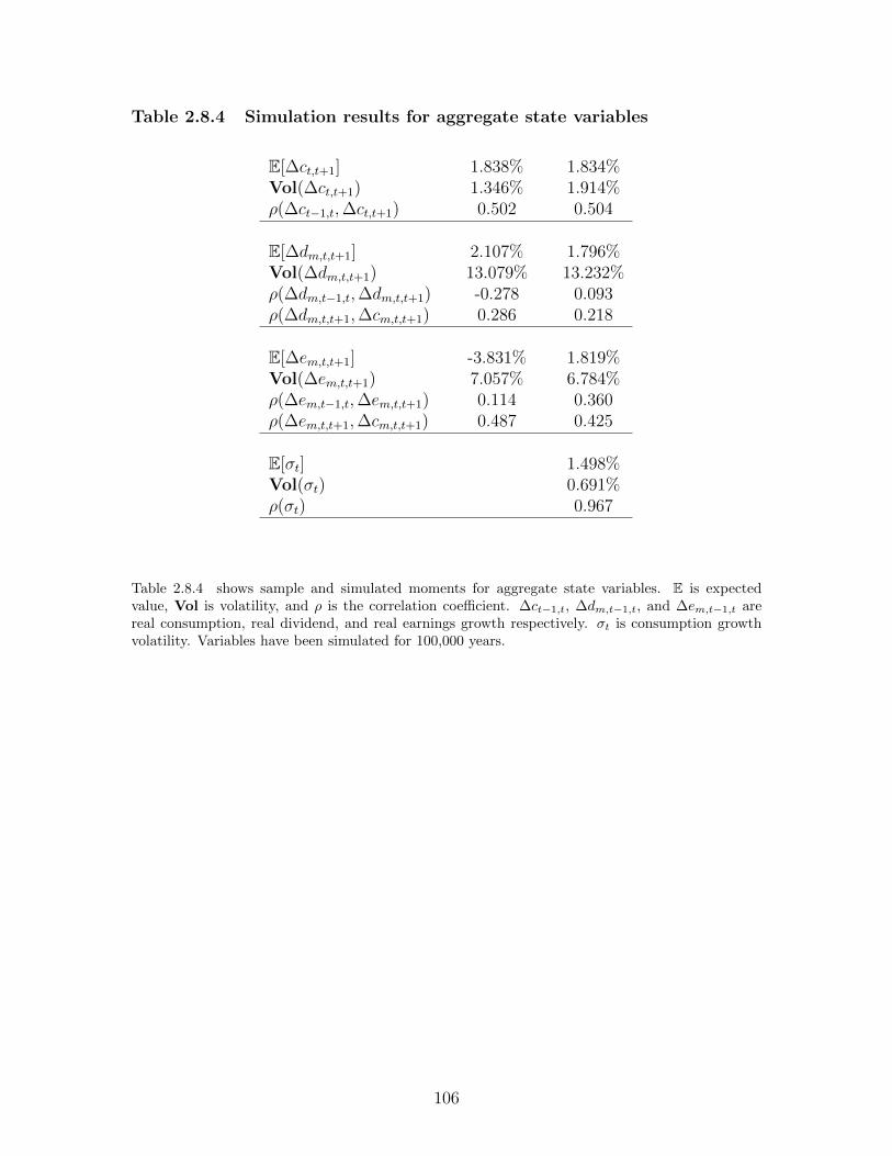
Table 2.8.4 Simulation results for aggregate state variables

E[∆ct,t+1] 1.838% 1.834%Vol(∆ct,t+1) 1.346% 1.914%ρ(∆ct−1,t,∆ct,t+1) 0.502 0.504

E[∆dm,t,t+1] 2.107% 1.796%Vol(∆dm,t,t+1) 13.079% 13.232%ρ(∆dm,t−1,t,∆dm,t,t+1) -0.278 0.093ρ(∆dm,t,t+1,∆cm,t,t+1) 0.286 0.218

E[∆em,t,t+1] -3.831% 1.819%Vol(∆em,t,t+1) 7.057% 6.784%ρ(∆em,t−1,t,∆em,t,t+1) 0.114 0.360ρ(∆em,t,t+1,∆cm,t,t+1) 0.487 0.425

E[σt] 1.498%Vol(σt) 0.691%ρ(σt) 0.967

Table 2.8.4 shows sample and simulated moments for aggregate state variables. E is expectedvalue, Vol is volatility, and ρ is the correlation coefficient. ∆ct−1,t, ∆dm,t−1,t, and ∆em,t−1,t arereal consumption, real dividend, and real earnings growth respectively. σt is consumption growthvolatility. Variables have been simulated for 100,000 years.

106

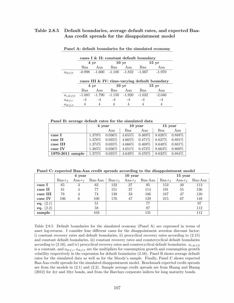
Table 2.8.5 Default boundaries, average default rates, and expected Baa-Aaa credit spreads for the disappointment model

Panel A: default boundaries for the simulated economy

cases I & II: constant default boundary4 yr 10 yr 15 yr

Baa Aaa Baa Aaa Baa Aaaadef,0 -0.998 -1.600 -1.108 -1.832 -1.007 -1.970

cases III & IV: time-varying default boundary4 yr 10 yr 15 yr

Baa Aaa Baa Aaa Baa Aaaai,def,0 -1.085 -1.790 -1.150 -1.920 -1.032 -2.040adef,c -4 -4 -4 -4 -4 -4adef,σ 4 4 4 4 4 4

Panel B: average default rates for the simulated data4 year 10 year 15 year

Aaa Baa Aaa Baa Aaacase I 1.379% 0.036% 4.655% 0.469% 8.626% 0.888%case II 1.378% 0.035% 4.665% 0.471% 8.627% 0.891%case III 1.374% 0.035% 4.666% 0.469% 8.640% 0.881%case IV 1.385% 0.036% 4.651% 0.472% 8.663% 0.869%1970-2011 sample 1.375% 0.035% 4.649% 0.476% 8.632% 0.884%

Panel C: expected Baa-Aaa credit spreads according to the disappointment model4 year 10 year 15 year

Baa-rf Aaa-rf Baa-Aaa Baa-rf Aaa-rf Baa-Aaa Baa-rf Aaa-rf Baa-Aaacase I 65 3 62 122 27 95 153 40 113case II 81 4 77 151 37 114 191 55 136case III 78 4 74 139 33 106 167 47 120case IV 106 6 100 176 47 129 215 67 148eq. (2.1) 51 77 97eq. (2.2) 58 87 112sample 103 131 112

Table 2.8.5 Default boundaries for the simulated economy (Panel A) are expressed in terms ofasset log-returns. I consider four different cases for the disappointment aversion discount factor:i) constant recovery rates and default boundaries, ii) procyclical recovery rates according to (2.15)and constant default boundaries, iii) constant recovery rates and countercyclical default boundariesaccording to (2.16), and iv) procyclical recovery rates and countercyclical default boundaries. ai,def,0is a constant, and adef,c, adef,σ are the multipliers for consumption growth and consumption growthvolatility respectively in the expression for default boundaries (2.16). Panel B shows average defaultrates for the simulated data as well as for the Moody’s sample. Finally, Panel C shows expectedBaa-Aaa credit spreads for the simulated disappointment model. Benchmark expected credit spreadsare from the models in (2.1) and (2.2). Sample average credit spreads are from Huang and Huang(2012) for 4yr and 10yr bonds, and from the Barclays corporate indices for long maturity bonds.

107

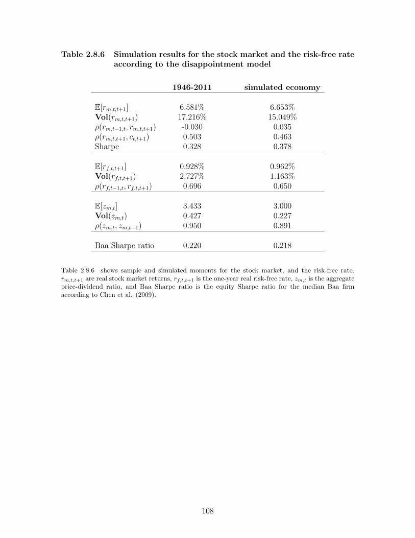
Table 2.8.6 Simulation results for the stock market and the risk-free rateaccording to the disappointment model

1946-2011 simulated economy

E[rm,t,t+1] 6.581% 6.653%Vol(rm,t,t+1) 17.216% 15.049%ρ(rm,t−1,t, rm,t,t+1) -0.030 0.035ρ(rm,t,t+1, ct,t+1) 0.503 0.463Sharpe 0.328 0.378

E[rf,t,t+1] 0.928% 0.962%Vol(rf,t,t+1) 2.727% 1.163%ρ(rf,t−1,t, rf,t,t+1) 0.696 0.650

E[zm,t] 3.433 3.000Vol(zm,t) 0.427 0.227ρ(zm,t, zm,t−1) 0.950 0.891

Baa Sharpe ratio 0.220 0.218

Table 2.8.6 shows sample and simulated moments for the stock market, and the risk-free rate.rm,t,t+1 are real stock market returns, rf,t,t+1 is the one-year real risk-free rate, zm,t is the aggregateprice-dividend ratio, and Baa Sharpe ratio is the equity Sharpe ratio for the median Baa firmaccording to Chen et al. (2009).

108

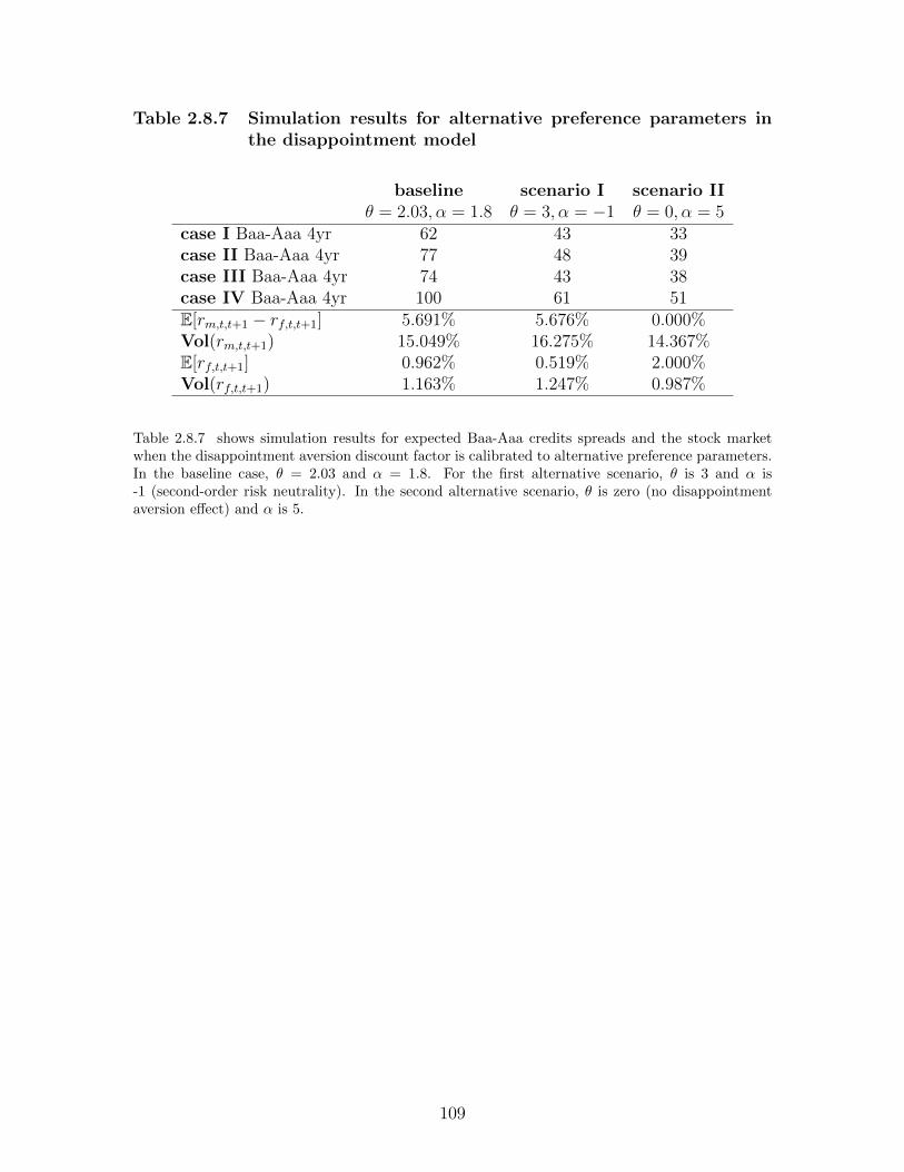
Table 2.8.7 Simulation results for alternative preference parameters inthe disappointment model

baseline scenario I scenario IIθ = 2.03, α = 1.8 θ = 3, α = −1 θ = 0, α = 5

case I Baa-Aaa 4yr 62 43 33case II Baa-Aaa 4yr 77 48 39case III Baa-Aaa 4yr 74 43 38case IV Baa-Aaa 4yr 100 61 51E[rm,t,t+1 − rf,t,t+1] 5.691% 5.676% 0.000%Vol(rm,t,t+1) 15.049% 16.275% 14.367%E[rf,t,t+1] 0.962% 0.519% 2.000%Vol(rf,t,t+1) 1.163% 1.247% 0.987%

Table 2.8.7 shows simulation results for expected Baa-Aaa credits spreads and the stock marketwhen the disappointment aversion discount factor is calibrated to alternative preference parameters.In the baseline case, θ = 2.03 and α = 1.8. For the first alternative scenario, θ is 3 and α is-1 (second-order risk neutrality). In the second alternative scenario, θ is zero (no disappointmentaversion effect) and α is 5.

109

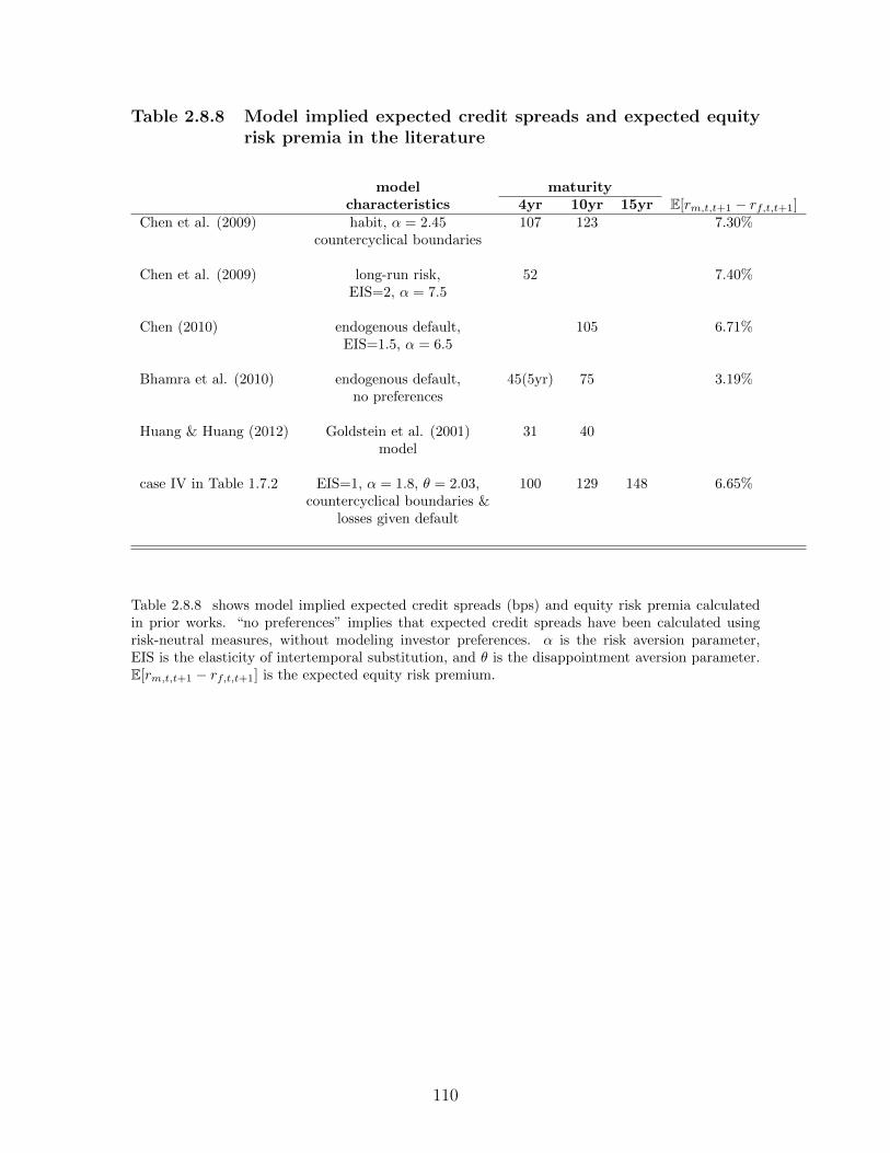
Table 2.8.8 Model implied expected credit spreads and expected equityrisk premia in the literature

model maturitycharacteristics 4yr 10yr 15yr E[rm,t,t+1 − rf,t,t+1]

Chen et al. (2009) habit, α = 2.45 107 123 7.30%countercyclical boundaries

Chen et al. (2009) long-run risk, 52 7.40%EIS=2, α = 7.5

Chen (2010) endogenous default, 105 6.71%EIS=1.5, α = 6.5

Bhamra et al. (2010) endogenous default, 45(5yr) 75 3.19%no preferences

Huang & Huang (2012) Goldstein et al. (2001) 31 40model

case IV in Table 1.7.2 EIS=1, α = 1.8, θ = 2.03, 100 129 148 6.65%countercyclical boundaries &

losses given default

Table 2.8.8 shows model implied expected credit spreads (bps) and equity risk premia calculatedin prior works. “no preferences” implies that expected credit spreads have been calculated usingrisk-neutral measures, without modeling investor preferences. α is the risk aversion parameter,EIS is the elasticity of intertemporal substitution, and θ is the disappointment aversion parameter.E[rm,t,t+1 − rf,t,t+1] is the expected equity risk premium.

110

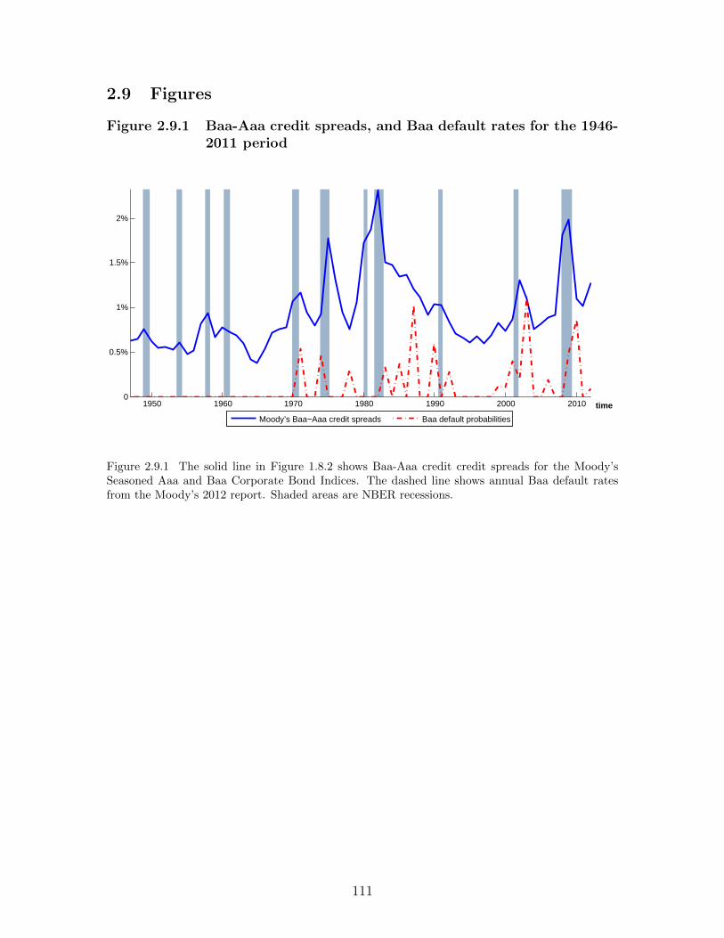
2.9 Figures

Figure 2.9.1 Baa-Aaa credit spreads, and Baa default rates for the 1946-2011 period

time

1950 1960 1970 1980 1990 2000 20100

0.5%

1%

1.5%

2%

Moody’s Baa−Aaa credit spreads Baa default probabilities

Student Version of MATLAB

Figure 2.9.1 The solid line in Figure 1.8.2 shows Baa-Aaa credit credit spreads for the Moody’sSeasoned Aaa and Baa Corporate Bond Indices. The dashed line shows annual Baa default ratesfrom the Moody’s 2012 report. Shaded areas are NBER recessions.

111

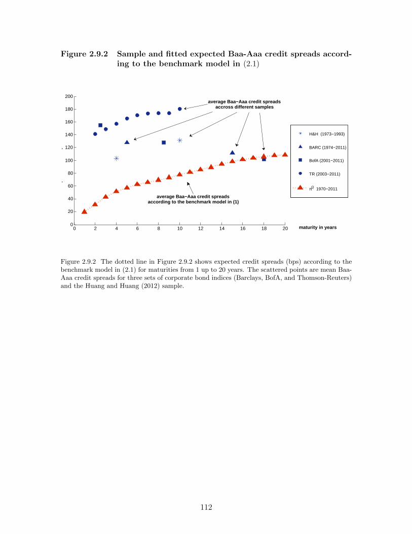
Figure 2.9.2 Sample and fitted expected Baa-Aaa credit spreads accord-ing to the benchmark model in (2.1)

0 2 4 6 8 10 12 14 16 18 200

20

40

60

80

100

120

140

160

180

200

expe

cted

cre

dit s

prea

ds

maturity in years

H&H (1973−1993)

BARC (1974−2011)

BofA (2001−2011)

TR (2003−2011)

πQ 1970−2011

average Baa−Aaa credit spreadsaccording to the benchmark model in (1)

average Baa−Aaa credit spreadsaccross different samples

Student Version of MATLAB

Figure 2.9.2 The dotted line in Figure 2.9.2 shows expected credit spreads (bps) according to thebenchmark model in (2.1) for maturities from 1 up to 20 years. The scattered points are mean Baa-Aaa credit spreads for three sets of corporate bond indices (Barclays, BofA, and Thomson-Reuters)and the Huang and Huang (2012) sample.

112

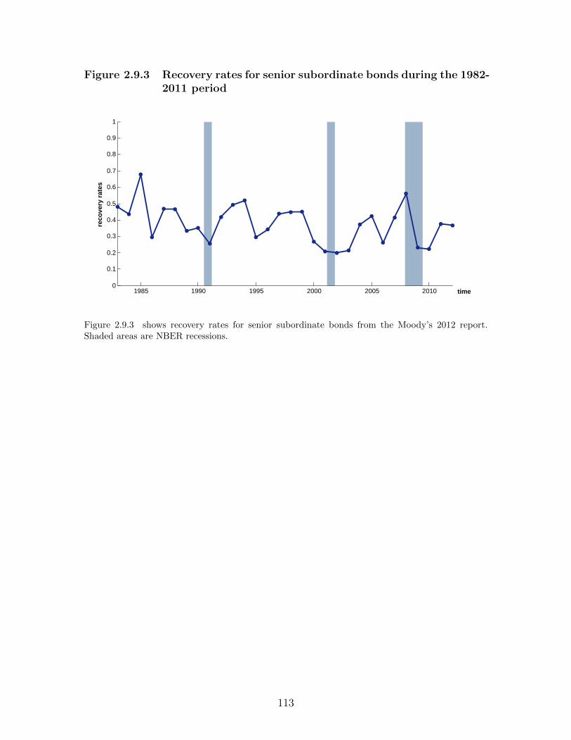
Figure 2.9.3 Recovery rates for senior subordinate bonds during the 1982-2011 period

reco

very

rat

es

time1985 1990 1995 2000 2005 20100

0.1

0.2

0.3

0.4

0.5

0.6

0.7

0.8

0.9

1

Student Version of MATLAB

Figure 2.9.3 shows recovery rates for senior subordinate bonds from the Moody’s 2012 report.Shaded areas are NBER recessions.

113

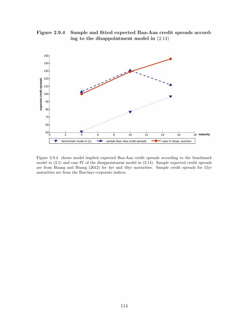
Figure 2.9.4 Sample and fitted expected Baa-Aaa credit spreads accord-ing to the disappointment model in (2.14)

0 2 4 6 8 10 12 14 16 1850

60

70

80

90

100

110

120

130

140

150

maturity

exp

ecte

d c

red

it s

pre

ads

benchmark model in (1) sample Baa−Aaa credit spreads case IV disap. aversion

Student Version of MATLAB

Figure 2.9.4 shows model implied expected Baa-Aaa credit spreads according to the benchmarkmodel in (2.1) and case IV of the disappointment model in (2.14). Sample expected credit spreadsare from Huang and Huang (2012) for 4yr and 10yr maturities. Sample credit spreads for 15yrmaturities are from the Barclays corporate indices.

114

APPENDICES

115

APPENDIX A

Disappointment Events in Consumption Growth,

and the Cross-Section of Expected Stock Returns

Appendix A.1 Preferences over stochastic payoffs

Assume that conditions for expected utility hold1. Suppose also that an investor

is endowed with $1, and is presented with the following dilemma: consume $1 for

sure or spend $1 to buy a ticket to a lottery that pays either $1 + σ or $1 − σ

(σ > 0) with equal probability. Consider first a risk-neutral agent whose preferences

over risky payoffs x can be expressed by a linear utility function U1(x) = x. Since

E[U1(x)] = U1

(E[x]

)= 1, the risk neutral agent is indifferent between taking the

actuarial fair bet or not.

Now suppose that preferences over risky payoffs x can be represented by a strictly

increasing, strictly concave, twice differentiable utility function U2(x) such that U2(1) =

1. The second-order Taylor approximation for expected utility 12U2(1+σ)+ 1

2U2(1−σ)

around the point σ0 = 0 is given by

1

2U2(1 + σ) +

1

2U2(1− σ) = U2(1) + 0.5U ′′2 (1)σ2 +O(σ3). (A.1)

1See von Neumann and Morgenstern (1944). For disappointment averse agents, the independenceaxiom can be relaxed with a betweenness axiom (Gul 1991).

116

Notice that when preferences are represented by smooth utility functions there are

no linear σ-terms in equation (A.1) because U2(x) is twice differentiable, and the

probability mass function for the random payoff is symmetric. Ignoring O(σ3) terms,

as long as U2(x) is strictly concave everywhere, then U ′′2 (x) < 0 ∀x, and 12U2(1 +σ) +

12U2(1 − σ) < U2(1) = 1. The risk averse individual would reject the lottery, unless

the lottery ticket were cheaper than $1 (risk premium2).

Taking the limit of the Taylor expansion in (A.1) as the variance becomes zero,

we conclude that

limσ2↓0

(U2(1) +

1

2U ′′2 (1)σ2 +O(σ3)

)= U2(1) = 1

When the dispersion of possible outcomes is very small, risk averse investors become

indifferent between participating in an actuarial fair lottery or not, much like a risk

neutral agent3.

The utility function for a loss averse individual is given by

U3(x) =

x+ θ(x− 1), x < 1, θ > 0,

x, x ≥ 1,

in which θ is the coefficient of loss aversion. Since loss aversion theory does not

provide any guidelines on the selection of the reference point, we set it equal to one,

the value of investor’s current wealth. Expected utility over lottery payoffs for the

loss averse individual is equal to

E[U3(x)] = 1− 1

2θσ.

For θ > 0, loss averse individuals would reject the fair bet, unless the ticket to enter

2The risk premium depends on the magnitude of U ′′2 (1) which is associated with the Arrow-Prattcoefficient of second-order risk aversion (Pratt 1964).

3See also the discussion in Backus et al. (2005) p. 334.

117

the lottery were cheaper than $1 (loss premium).

Consider finally an individual whose preferences over payoffs are described by a

utility function of the form

U4(x;µ) =

x+ θ(x− µ), x < µ, θ > 0, µ = E[x]

+ E[θ(x− µ)1{x < µ}

],

x, x ≥ µ,

in which θ > 0 is the coefficient of disappointment aversion, and µ is the certainty

equivalent of the random payoff4. Notice that µ is also the threshold for disappoint-

ment events. For θ > 0, µ ∈ (1− σ, 1 + σ) and in particular

µ = 1−12θ

1 + 12θσ < 1. (A.2)

The disappointment averse agent would also reject the actuarially fair bet, unless the

price to enter the lottery were cheaper than $1 (disappointment premium).

Let ε be an extremely small positive number close to zero, and consider the limit

in (A.2) as σ2 approaches ε

limσ2↓ε

µ = 1−12θ

1 + 12θ

√ε < 1.

A similar expression holds for loss averse individuals

limσ2↓ε

(1− 1

2θ√σ2)

= 1− 1

2θ√ε < 1.

4According the the generalized disappointment aversion model of Routledge and Zin (2010), thereference level for gains and losses is a multiple δ of the certainty equivalent µ

U4(x;µ) =

{x+ θ(x− δµ), x < δµ, δ ∈ (0, 1], θ > 0, µ = E

[x]

+ E[θ(x− δµ)1{x < δµ}

],

x, x ≥ δµ.

For the case δ > 1, the reader is referred to Routledge and Zin (2010).

118

Finally, for the continuously differentiable concave utility function, it follows that

limσ2↓ε

(U2(1) +

1

2U ′′2 (1)σ2 +O(σ3)

)= U2(1) +

1

2U ′′2 (1)ε ≈ 1.

As σ2 approaches zero, σ also approaches zero but at a far slower rate than σ2 5.

First-order risk aversion effects in disappointment or loss aversion preferences do

not vanish immediately as σ2 ↓ 0. In contrast, as σ2 ↓ 0, a second-order risk averse

individual would be indifferent between accepting actuarial fair lotteries or not. When

the dispersion of lottery payoffs is small, first-order risk aversion induces a more

conservative risk taking behavior than second-order risk aversion.

In the context of consumption-based asset pricing, smooth utility functions need

to be extremely concave in order to generate realistic equity risk premia because

aggregate consumption growth exhibits very low variability (σ2c ↓ 0). On the other

hand, even if consumption growth variance is almost zero, there might still be mea-

surable consumption growth volatility terms (σc > 0). These volatility terms can

be combined with disappointment aversion preferences to generate measurable equity

risk premia.

The figure below shows utility plots for all four types of preferences considered

here. When uncertainty is low, linear utility becomes tangential to the CRRA utility

function, and CRRA investors behave as if they were risk-neutral.

Appendix A.2 Linear disappointment aversion preferences

One of the key insights of non-separable utility functions is that preferences over

the timing and uncertainty of payoffs need not be characterized by the same param-

eter. The disappointment aversion framework can separate preferences over risk and

time, while preserving the additive form for lifetime utility Vt. Suppose that in equa-

5σ approaches zero at a square root rate, yet as σ2 eventually becomes zero, σ will also becomezero.

119

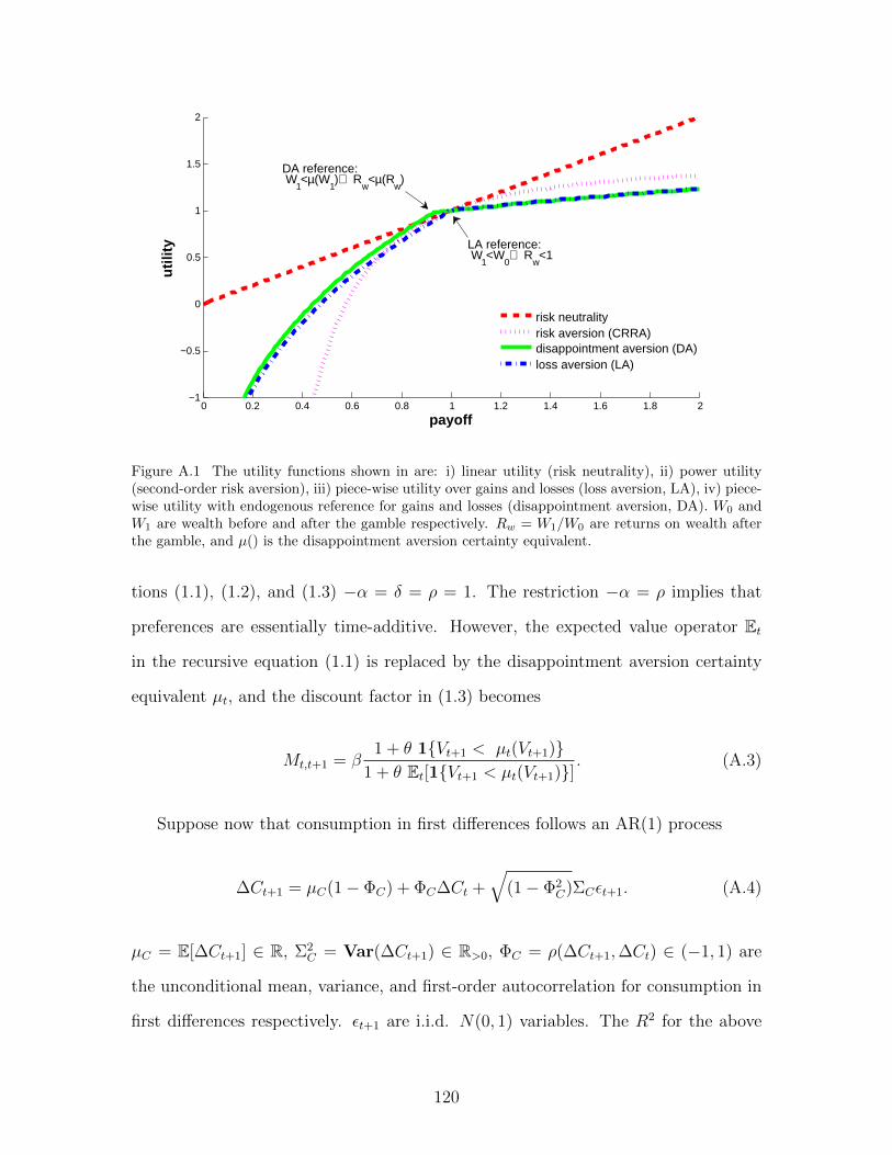
0 0.2 0.4 0.6 0.8 1 1.2 1.4 1.6 1.8 2−1

−0.5

0

0.5

1

1.5

2

payoff

uti

lity

risk neutralityrisk aversion (CRRA)disappointment aversion (DA)loss aversion (LA)

DA reference: W

1<µ(W

1)⇒ R

w<µ(R

w)

LA reference: W

1<W

0⇒ R

w<1

Student Version of MATLAB

Figure A.1 The utility functions shown in are: i) linear utility (risk neutrality), ii) power utility(second-order risk aversion), iii) piece-wise utility over gains and losses (loss aversion, LA), iv) piece-wise utility with endogenous reference for gains and losses (disappointment aversion, DA). W0 andW1 are wealth before and after the gamble respectively. Rw = W1/W0 are returns on wealth afterthe gamble, and µ() is the disappointment aversion certainty equivalent.

tions (1.1), (1.2), and (1.3) −α = δ = ρ = 1. The restriction −α = ρ implies that

preferences are essentially time-additive. However, the expected value operator Et

in the recursive equation (1.1) is replaced by the disappointment aversion certainty

equivalent µt, and the discount factor in (1.3) becomes

Mt,t+1 = β1 + θ 1{Vt+1 < µt(Vt+1)}

1 + θ Et[1{Vt+1 < µt(Vt+1)}]. (A.3)

Suppose now that consumption in first differences follows an AR(1) process

∆Ct+1 = µC(1− ΦC) + ΦC∆Ct +√

(1− Φ2C)ΣCεt+1. (A.4)

µC = E[∆Ct+1] ∈ R, Σ2C = Var(∆Ct+1) ∈ R>0, ΦC = ρ(∆Ct+1,∆Ct) ∈ (−1, 1) are

the unconditional mean, variance, and first-order autocorrelation for consumption in

first differences respectively. εt+1 are i.i.d. N(0, 1) variables. The R2 for the above

120

AR(1) model is 24.571% at the annual frequency, and 25.909% for quarterly data.

Since Vt+1 is unobservable, the use of the disappointment aversion discount factor in

(A.3) for empirical purposes becomes problematic. However, we can express lifetime

utility Vt in terms of consumption changes ∆Ct,

Proposition 2: Given the consumption dynamics in (A.4), then for −α = ρ = δ = 1

in equations (1.1), (1.2) and (1.3), investors’ lifetime utility Vt can be expressed as

Vt = Ct + µV + ΦV ∆Ct ∀t, where

• ΦV = βΦC1−βΦC

, ΦV ∈ R,

• µV = β1−β

[µC(1− ΦC)(ΦV + 1)− θn(d1)

1+θN(d1)(ΦV + 1)

√1− Φ2

CΣC

], µV ∈ R,

• d1 ∈ R<0 is the solution to the fixed point problem

d1 = − θn(d1)

1 + θN(d1), (A.5)

and N(.) and n(.) are the standard normal cdf and pdf respectively.

Proof. See Appendix A.4.2.

Proposition 2 tells us that lifetime utility minus current consumption (Vt − Ct)

is an affine function of consumption in first differences (∆Ct). µV is the constant

term, and ΦV is the slope coefficient for consumption changes. Notice the linear

(d1

√1− Φ2

CΣC), instead of quadratic, structure of the disappointment aversion cor-

rection in µv. Comparative statics for µV imply that high uncertainty about the

economy (large ΣC) or a large disappointment aversion coefficient θ would lead to

large (in absolute magnitude) corrections to µV6.

6∂µV /∂θ = − n(d1)1+θN(d1)

(1− θN(d1)

1+θN(d1)

)< 0 since the inequality 1 > x

1+x holds trivially ∀ x ∈ R>0.

121

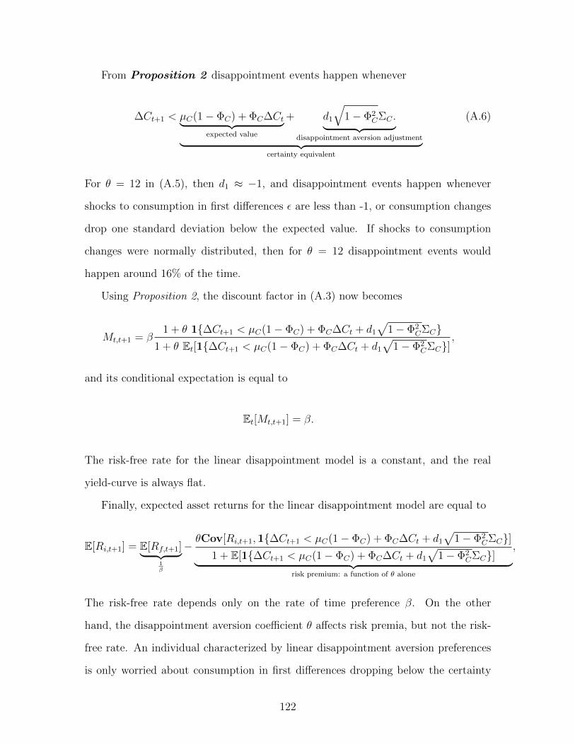
From Proposition 2 disappointment events happen whenever

∆Ct+1 < µC(1− ΦC) + ΦC∆Ct︸ ︷︷ ︸expected value

+ d1

√1− Φ2

CΣC .︸ ︷︷ ︸disappointment aversion adjustment︸ ︷︷ ︸

certainty equivalent

(A.6)

For θ = 12 in (A.5), then d1 ≈ −1, and disappointment events happen whenever

shocks to consumption in first differences ε are less than -1, or consumption changes

drop one standard deviation below the expected value. If shocks to consumption

changes were normally distributed, then for θ = 12 disappointment events would

happen around 16% of the time.

Using Proposition 2, the discount factor in (A.3) now becomes

Mt,t+1 = β1 + θ 1{∆Ct+1 < µC(1− ΦC) + ΦC∆Ct + d1

√1− Φ2

CΣC}1 + θ Et[1{∆Ct+1 < µC(1− ΦC) + ΦC∆Ct + d1

√1− Φ2

CΣC}],

and its conditional expectation is equal to

Et[Mt,t+1] = β.

The risk-free rate for the linear disappointment model is a constant, and the real

yield-curve is always flat.

Finally, expected asset returns for the linear disappointment model are equal to

E[Ri,t+1] = E[Rf,t+1]︸ ︷︷ ︸1β

−θCov[Ri,t+1,1{∆Ct+1 < µC(1− ΦC) + ΦC∆Ct + d1

√1− Φ2

CΣC}]1 + E[1{∆Ct+1 < µC(1− ΦC) + ΦC∆Ct + d1

√1− Φ2

CΣC}]︸ ︷︷ ︸risk premium: a function of θ alone

,

The risk-free rate depends only on the rate of time preference β. On the other

hand, the disappointment aversion coefficient θ affects risk premia, but not the risk-

free rate. An individual characterized by linear disappointment aversion preferences

is only worried about consumption in first differences dropping below the certainty

122

equivalent. On the other hand, an investor with log-linear disappointment aversion

preferences (section 1.3.2) cares about consumption growth falling below the certainty

equivalent, as well as about the actual level of consumption growth.

Appendix A.3 Consistency and asymptotic normality of GMM estima-

tors when the GMM objective function is not continuous

In order to prove consistency and asymptotic normality for GMM estimators, stan-

dard applications require differentiability of the GMM objective function. However,

continuity and differentiability are violated when moment restrictions are associated

with indicator functions.

Let zt be a vector of random variables and x a vector of parameters. Consider the

GMM objective function

Q0 = E[q(zt, x)

]′W E

[q(zt, x)

], (A.7)

and its sample analogue

QT =[ 1

T

T∑t=1

q(zt, x)]′W[ 1

T

T∑t=1

q(zt, x)]. (A.8)

For the disappointment aversion model x = {β, α, θ}, zt ={

∆ct+1, {ri,t+1}n−1i=1 , rf,t+1

},

and

q(zt, θ) = Mt,t+1

(eri,t+1 − erf,t+1

)for i = 1, 2, ..., n, (A.9)

123

with

Mt,t+1 = exp[log(β) + α(φv + 1)µc(1− φc)−

α2

2(φv + 1)2(1− φ2

c)σ2c

−[α(φv + 1) + 1]∆ct+1 +α

βφv∆ct

](1 + θ1{∆ct+1 < µc(1− φc) + φc∆ct + d1

√1− φ2

cσc}),

and

d1 = −α2

(φv + 1)√

1− φ2cσc −

1

α(φv + 1)√

1− φ2cσc

log[1 + θN

(d1 + α(φv + 1)

√1− φ2

cσc)

1 + θN(d1

) ].

We can assume that x = {β, α, θ} takes values in a compact space X ∈ R3.

Economic theory suggests that for disappointment averse investors β ∈ (0, 1), α ∈

(−1, Bα), and θ ∈ (0, Bθ). Bα < +∞ and Bθ < +∞ are upper bounds for the coef-

ficients of risk and disappointment aversion respectively. In general, risk preference

parameters α and θ cannot assume infinite values, and are bounded from above by

some positive real numbers (Bα and Bθ) which may be arbitrarily large but finite. We

will also assume that zt ={

∆ct+1, {ri,t+1}n−1i=1 , rf,t+1

}is characterized by a continu-

ous probability distribution function, and a well-defined moment generating function

∀x ∈ X7. Finally, let x0 be the minimizer in (A.7), and xT the minimizer in (A.8).

Identification. We will assume that the GMM objective function in (A.7) satis-

fies the conditions in Lemma 2.3, p. 2126 in Newey and McFadden (1994), so that x0

is globally identified. Because it is quite hard to verify identification, for the practical

purposes of our estimation we will simply assume it8.

Consistency. For consistency of GMM estimators when the GMM objective

function is not continuous, we refer to Theorem 2.6, p. 2132 in Newey and McFadden

(1994). We essentially require that:

1. zt is stationary and ergodic

7For β ∈ (0, 1) and ∆ct+1 stationary, it also follows that 1− φcβ 6= 0.8See also the discussion in Newey and McFadden (1994), p. 2127 on the Hansen and Singleton

(1982) model.

124

2. Wp→W , W is positive definite, and WE[g(z, x0)] = 0 only if x = x0

3. X is compact

4. q(zt, x) is continuous with probability one.

5. E[supx∈X||q(zt, x)||

]< +∞

Stationarity and ergodicity are reasonable properties for the random variables{∆ct+1, {ri,t+1}n−1

i=1 , rf,t+1

}at the quarterly and annual frequencies. The second con-

dition is satisfied because the GMM weighting matrix is constant, and equal to the

identity matrix. Moreover, according to the identification assumption above, the

GMM objective function has a unique minimizer x0 which can be identified. Eco-

nomic theory suggests that the parameter space X is compact. The fourth condition

is also satisfied since the only point of discontinuity in expression (A.9) is

∆ct+1 = φc∆ct + µc(1− φc) + d1

√1− φ2

cσc,

which is a zero-probability event as long as consumption growth is a continuous

random variable. Finally, condition five is satisfied because X is compact, and the

distribution of zt has a well-defined moment generating function ∀x ∈ X.

Asymptotic normality. Theorems 7.2, p. 2186, and 7.3, p. 2188 in Newey and

McFadden (1994) provide conditions for asymptotic normality of GMM estimates

when the GMM objective function is not continuous. These conditions are

1.[

1T

∑Tt=1 q(zt, x)

]′W[

1T

∑Tt=1 q(zt, x)

]≤ infx∈X

[1T

∑Tt=1 q(zt, x)

]′W[

1T

∑Tt=1 q(zt, x)

]2. W

p→W , W is positive definite

3. xp→x0

125

4. x0 is in the interior of X

5. E[g(z, x0)] = 0

6.[

1T

∑Tt=1 q(zt, x0)

] d→N(0,Σ)

7. E[g(z, x)] is differentiable at x0 with derivative G, and G′WG is non-singular

8. for δN → 0, then

sup||x−x0||≤δn

√n∣∣∣∣∣∣[ 1

T

∑Tt=1 q(zt, x)

]−[

1T

∑Tt=1 q(zt, x0)

]− E

[g(z, x0)

]∣∣∣∣∣∣1 +√n||x− x0||

p→ 0. (A.10)

The first condition is related to identification. The second condition is satisfied since

W = I. The third condition is satisfied by the consistency theorem above. Condi-

tions 4, 5, and 6 are standard GMM assumptions. The seventh condition is satisfied

provided that the joint probability density function of asset returns and consumption

growth is continuous, and that the moment generating function is well-defined. The

critical condition for asymptotic normality is condition 8, the stochastic equicontinu-

ity condition.

Andrews (1994) provides primitive conditions in order to verify stochastic equicon-

tinuity. These conditions are related to Pollard’s entropy condition (Pollard 1984).

Fortunately, the GMM objective function in (A.9) is a mixture of functions that sat-

isfy the entropy condition. According to Theorem 2, p. 2272 in Andrews (1994),

indicator functions (which are “type I” functions, p. 2270 in Andrews 1994) sat-

isfy Pollard’s conditions. A second class of functions (“type II” functions, p. 2271

in Andrews 1994) that satisfy Pollard’s conditions are functions which depend on

a finite number of parameters, and are Lipschitz-continuous9 with respect to these

parameters.

9Lipschitz continuity is also exploited in Theorem 7.3, p. 2188, in Newey and McFadden (1994)as a primitive condition to show stochastic equicontinuity.

126

The GMM q(zt, x) vector-valued function in equation (A.9) consists of exponen-

tial terms which, in turn, are functions of a finite number of preference parameters.

Exponentially functions are only locally Lipschitz-continuous. However, the exponen-

tial terms in the GMM objective function are Lipschitz-continuous on the compact

parameter space X, since the rate of change of the exponential functions remains

bounded as long as variables take values in compact spaces. Therefore, exponential

functions defined on the compact set X belong to the “type II” class of functions.

We conclude that the disappointment aversion GMM objective function in equation

(A.9) contains terms which individually satisfy Pollard’s entropy condition.

According to Theorem 3, p. 2273 in Andrews (1994), elementary operations among

“type I” and “type II” functions result in functions which also satisfy Pollard’s en-

tropy condition. Consequently, the disappointment aversion GMM objective function

in (A.9), which is a product of “type I” and “type II” functions, satisfies the stochas-

tic equicontinuity condition, and GMM estimates for the disappointment model are

therefore asymptotically normally distributed.

The above discussion confirms that even though q(zt, x) in (A.9) is not continuous

with respect to x = {β, α, θ}, standard results from GMM asymptotic theory can still

be applied provided that certain regularity conditions are satisfied. These conditions

are in general associated with “continuity” and “differentiability” of the function

E[q(zt, x)

]rather than the function q(zt, x) itself.

Finally, even if q(zt, x) is not continuous or continuously differentiable, we can still

proceed with hypothesis testing as usual by replacing derivatives with finite differ-

ences approximations. Theorem 7.4, p. 2190 in Newey and McFadden (1994) suggests

that numerical derivatives for 1T

∑Tt=1 q(zt, x) will asymptotically converge in proba-

bility to the derivative of E[q(zt, x)]. We can, therefore, obtain consistent asymptotic

variance estimators using finite differences. However, a practical problem with nu-

merical derivatives is the choice of perturbation parameters used in the denominator.

127

Unfortunately, econometric theory does not provide a clear answer to this problem.

Appendix A.4 Proofs

Appendix A.4.1 Proof of Proposition 1

For ρ = 0 and δ = 1, equation (1.1) implies that along an optimal consumption path10

(VtCt

) 1β

= µt(Vt+1

Ct;Vt+1

Ct< µt(

Vt+1

Ct)).

Taking logs in both sides of the equation, and using the definition of the disappoint-

ment aversion certainty equivalent µt in (1.2), we obtain

1

β(vt − ct) = − 1

αlogEt

{exp[− α(vt+1 − ct)

] 1 + θ1{vt+1 − ct < 1β(vt − ct)}

1 + θEt[1{vt+1 − ct < 1β(vt − ct)}]

}.

Letting vt − ct = µv + φv∆ct ∀t, then

1

β(µv + φv∆ct) = − 1

αlogEt

{e−α[µv+(φv+1)∆ct+1

] 1 + θ1{µv + (φv + 1)∆ct+1 <1β(µv + φv∆ct)}

1 + θEt[1{µv + (φv + 1)∆ct+1 <1β(µv + φv∆ct)}]

}.

We can use (1.5) to express ∆ct+1 in terms of ∆ct

1β(µv + φv∆ct) = − 1

αlogEt

{exp[− α

[µv + (φv + 1)

(µc(1− φc) + φc∆ct +

√1− φ2

cσcεt)]]×

1+θ1{µv+(φv+1)(µc(1−φc)+φc∆ct+√

1−φ2cσcεt+1)< 1

β(µv+φv∆ct)}

1+θEt[1{µv+(φv+1)(µc(1−φc)+φc∆ct+√

1−φ2cσcεt+1)< 1

β(µv+φv∆ct)}]

}.

Partial moments for log-normal random variables imply that

1β(µv + φv∆ct) = µv + (φv + 1)

(µc(1− φc) + φc∆ct − α

2(φv + 1)2(1− φ2

c)σ2c

)(A.11)

− 1αlog[1 + θN

( 1β

(µv+φv∆ct)−µv−(φv+1)(µc(1−φc)+φc∆ct)

(φv+1)√

1−φ2cσc

+ α(φv + 1)√

1− φ2cσc

)]+ 1αlog[1 + θN

( 1β

(µv+φv∆ct)−µv−(φv+1)(µc(1−φc)+φc∆ct)

(φv+1)√

1−φ2cσc

)].

10Lower case letters denote logs of variables.

128

Ignoring for the moment the last two log-terms, φv must satisfy

φv =βφc

1− βφc.

For φv = βφc1−βφc , the two log-terms in (A.11) do not depend on ∆ct. Hence, the

constant term µv in (A.11) must be equal to

µv =β

1− β

{µc(1− φc)1− βφc

− α(1− φ2c)σ

2c

2(1− βφc)2

− 1

αlog[1 + θN

( 1−ββµv−(φv+1)µc(1−φc)

(φv+1)√

1−φ2cσc

+ α(φv + 1)√

1− φ2cσc

)1 + θN

( 1−ββµv−(φv+1)µc(1−φc)

(φv+1)√

1−φ2cσc

) ]}.

We can define the disappointment event threshold as11

d1 =

1−ββµv − (φv + 1)µc(1− φc)(φv + 1)

√1− φ2

cσc. (A.12)

Then µv becomes

µv =β

1− β

{(φv + 1)µc(1− φc)−

α

2(φv + 1)2(1− φ2

c)σ2c

− 1

αlog[1 + θN

(d1 + α(φv + 1)

√1− φ2

cσc)

1 + θN(d1

) ]}.

Plugging back the above expression for µv into the definition of d1 in (A.12), d1 is the

solution to the fixed-point problem

d1 = −α2

(φv + 1)√

1− φ2cσc −

1

α(φv + 1)√

1− φ2cσc

log[1 + θN

(d1 + α(φv + 1)

√1− φ2

cσc)

1 + θN(d1

) ].

11If δ 6= 1 in (1.2), then d1 would be a function of ∆ct, and the linearity of the log-value functionin terms of consumption growth would brake down.

129

Finally,

µv =β

1− β

{(φv + 1)µc(1− φc) + d1(φv + 1)

√1− φ2

cσc

}.

Appendix A.4.2 Proof of Proposition 2

For −α = ρ = δ = 1, equation (1.1) implies that along an optimal consumption path

1

β

(Vt − Ct

)= µt

(Vt+1 − Ct; Vt+1 − Ct <

1

β

(Vt − Ct

)).

Assume that Vt − Ct = µV + ΦV ∆Ct ∀t, then

1

β

(µV + ΦV ∆Ct

)= µt

(µV + (ΦV + 1)∆Ct+1; µV + (ΦV + 1)∆Ct+1 <

1

β[µV + ΦV ∆Ct]

).

Plugging the dynamics for ∆Ct+1 from equation (A.4), it follows that

1

β

(µV + ΦV ∆Ct

)= Et

[(µV + (ΦV + 1)µC + (ΦV + 1)ΦC∆Ct + (ΦV + 1)ΣCεt+1

)(1 + θ1{µV + (ΦV + 1)µC + (ΦV + 1)ΦC∆Ct + (ΦV + 1)ΣCεt+1 <

1

β(µV + ΦV ∆Ct)}

)]×{

1 + θEt[1{µV + (ΦV + 1)µC + (ΦV + 1)ΦC∆Ct + (ΦV + 1)ΣCεt+1 <

1

β(µV + ΦV ∆Ct)}

]}−1

,

where µC = µc(1 − ΦC) and ΣC = Σc

√1− Φ2

C . Since error terms εt+1 are normally

distributed, we conclude that12

1

β

(µV + ΦV ∆Ct

)=

1

1 + θ N(d1)×{µV + (ΦV + 1)µC (A.13)

+(ΦV + 1)ΦC∆Ct + θ[(µV + (ΦV + 1)µC + (ΦV + 1)ΦC∆Ct

)N(d1)

]− θ n(d1)

(ΦV + 1

)ΣC

},

12Winkler et al. (1972) derive simple expressions for partial moments of normally and log-normally distributed random variables.

130

in which N(.) and n() are the standard normal c.d.f. and p.d.f. respectively, and

d1 =[ 1

β(µV + ΦV ∆Ct)− µV − (ΦV + 1)µC − (ΦV + 1)ΦC∆Ct

]·((ΦV + 1)ΣC

)−1, (A.14)

is the disappointment threshold.

Equation (A.13) simplifies to

1

β

(µV + ΦV ∆Ct

)=[µV + µC(ΦV + 1) + (ΦV + 1)ΦC∆Ct

]−θn(d1)

(ΦV + 1

)ΣC

1 + θ N(d1). (A.15)

Ignoring for the moment the last term, ΦV must satisfy

ΦV =βΦC

1− βΦC

.

For ΦV = βΦC1−βΦC

13, then d1 in (A.14) is equal to

d1 =[1− β

βµV − (ΦV + 1)µC

]·((ΦV + 1)ΣC

)−1. (A.16)

Thus, for ΦV = βΦC1−βΦC

, there are no ∆Ct terms in the expression for the disappoint-

ment threshold d1. Collecting constant terms from (A.15), µv is equal to

µV =β

1− β[(ΦV + 1)µC(1− ΦC)− θn(d1)

1 + θN(d1)

√1− Φ2

C(ΦV + 1)ΣC

].

Plugging the equation for µV back into the equation for d1 in (A.16), d1 now becomes

the solution to the fixed point problem14

d1 = − θn(d1)

1 + θN(d1)< 0. (A.17)

13The scalar 1− βΦC is non-zero since ΦC lies within the (−1, 1) interval, and β ∈ (0, 1).14Given the continuity and monotonicity of the function h(x) = x+ θn(x)

1+θN(x) for θ > 0, the fixed

point problem is well defined and has a negative solution.

131

APPENDIX B

Disappointment Aversion Preferences, and the

Credit Spread Puzzle

Appendix B.1 Bond yields according to the benchmark model in (2.1)

Suppose that single-period, cum-payout, asset log-returns for firm i ri,t,t+1 are

i.i.d. normal random variables with constant mean µi − 12σ2i ∈ R, and volatility

σi ∈ R>0. Let ∆i be the constant log-payout yield(∆i = log(1 +

Oi,t+1

Pi,t+1))

1. Ex-

payout, log-returns rxi,t,t+1 are equal to cum-payout log-returns minus the log-payout

yield (rxi,t,t+1 = ri,t,t+1−∆i). Hence, rxi,t,t+1 are also normal random variables, and, in

a discrete-time setting, can be expressed as

rxi,t,t+1 = µi −∆i −1

2σ2i + σiεi,t+1,

with εi,t+1 i.i.d. N(0, 1) shocks. Moreover, T -period, ex-payout returns are also i.i.d.

normal random variables with mean (µi −∆i − 12σ2i )T and volatility σi

√T .

Suppose that the single-period, log risk-free rate is constant and equal to rf .

Assume also that there are no taxes, and that default boundaries Di,T as well as

1Oi,t+1 is the payout, and Pi,t+1 is the price of assets in place.

132

losses given default L are constant. Let πPi,t,t+T be the physical probability of default

for a T -period, zero-coupon bond

πPi,t,t+T = Pt

(Pi,t+T < Di,T

).

Pi,t is the value of assets in place for firm i. Similarly to the original Merton model,

default can only happen at the expiration date t + T , but unlike the Merton model,

the default boundary is not necessarily equal to the face value of debt. Normalizing

current period firm value Pi,t to one, the physical probability of default πPi,t,t+T can

be expressed in terms of asset log-returns rxi,t,t+1

πPi,t,t+T = N

( logDi,T − (µi −∆i − 12σ2i )T

σi√T

),

in which N() is the standard normal c.d.f.. Because asset log-returns are i.i.d. with

constant mean and standard deviation, πPi,t,t+T depends only on maturity T , hence

πPi,t,t+T = πP

i,T . Finally, using the inverse of the normal c.d.f. N−1(), we can express

the log-default boundary logDi,T in terms of the physical probability of default πPi,T ,

expected returns for assets in place µi, and asset return volatility σi

logDi,T = (µi −∆i −1

2σ2i )T +N−1

(πPi,T

)σi√T . (B.1)

The continuous-time framework in Black and Scholes (1973) allows for frictionless

trading and hedging between underlying and derivative securities. An immediate

consequence of continuous trading is that if asset returns under the physical measure

are normally distributed with constant mean and volatility, then asset returns under

the risk-neutral measure are also normally distributed with the same variance, and

mean equal to the risk-free rate.

In a discrete-time setting, continuous trading is not possible. However, according

133

to Lemma 1 in Appendix B.6.1, the risk-neutral density for asset returns is normal,

provided that aggregate preferences over consumption are described by a CRRA util-

ity function, and that aggregate consumption growth is a log-normal random vari-

able. Hence, assuming that all conditions for Lemma 1 hold, T -period, ex-payout

asset log-returns under the risk-neutral measure are normally distributed with mean

(rf −∆i − 12σ2i )T , and volatility σi

√T .

Let yi,t,t+T be the continuously compounded yield to maturity for a T -period,

zero-coupon bond written on firm i at time t. Then, under the risk-neutral measure

e−Tyi,t,t+T = e−Trf(

1− LN( logDi,T − (rf −∆i − 1

2σ2i )T

σi√T

)). (B.2)

Taking logs in (B.2), and substituting logDi,T with the expression from (B.1), we get

that

yi,t,t+T − rf = − 1

Tlog[1− LN

(N−1

(πPi,T

)+µi − rfσi

√T)].

Since the right-hand side above and the risk-free rate are constants, we conclude that

E[yi,t,t+T ]− rf = − 1

Tlog[1− LN

(N−1

(πPi,T

)+µi − rfσi

√T)].

Appendix B.2 Bond yields according to the model in (2.2) with time-

varying recovery rates

Suppose that recovery rates are the same across all bonds, and depend only on

consumption growth

1− Lt+T = arec,0 + arec,c∆ct+T−1,t+T .

134

Suppose also that all the assumptions in Appendix B.1 hold. Then, the yield-to-

maturity for a zero-coupon, T-period bond is given by2

e−Tyi,t,t+T = e−TrfEQt

[EQt

[1− (1− arec,0 − arec,c∆ct+T−1,t+T )1

{ri,t,t+T < logDi,T

}|∆ct+T−1,t+T

]],

in which EQt is the expectation under the risk-neutral measure. Further algebra implies

that

e−Tyi,t,t+T = e−TrfEQt

[1− (1− arec,0 − arec,c∆ct+T−1,t+T )N

( logDi,T − (rf −∆i − 12σ2i )T

σi√T

)]

According to Appendix B.6.3, under the risk neutral measure, log-consumption

growth is a normal random variable with volatility σc, and mean µc− µm−rfρm,cσm

σc.µm−rfσm

is the stock market Sharpe ratio, and ρm,c is the correlation between stock market

returns and consumption growth. Using the expression for the default boundary

logDi,T from (B.1), we obtain

e−T (yi,t,t+T+rf ) =[1−

(1− arec,0 − arec,cµc︸ ︷︷ ︸

E[Lt+T ]

+arec,cµm − rfρm,cσm

σc

)N(N−1

(πPi,T

)+µi − rfσi

√T)].

Since the right-hand side and the risk-free rate are constants, we conclude that

E[yi,t,t+T ]− rf = − 1

Tlog[1−

(E[Lt+T ] + arec,c

µm − rfρm,cσm

σc

)N(N−1

(πPi,T

)+µi − rfσi

√T)].

2Under the risk neutral measure Q, asset returns ri,t,t+1 and consumption growth are indepen-dent.

135

Appendix B.3 Intertemporal marginal rate of substitution for disappoint-

ment aversion preferences

Along an optimal consumption path, the Bellman equation for the representative

investor’s consumption-investment problem implies that

Vt =[(1− β)Cρ

t + βµt(Vt+1

)ρ] 1ρ ,

where µt is the disappointment aversion certainty equivalent from (2.4). The expres-

sion for the stochastic discount factor is given by

Mt,t+1 =∂Vt/∂Ct+1

∂Vt/∂Ct,

in which

∂Vt/∂Ct =1

ρV 1−ρt (1− β)ρCρ−1

t ,

and

∂Vt/∂Ct+1 =1

ρV 1−ρt βρµt

(Vt+1

)ρ−1 ×

(− 1

α)Et[ V −αt+1 (1 + θ1{Vt+1 < δµt})

1− θ(δ−α − 1)1{δ > 1}+ θδ−αEt[1{Vt+1 < δµt}]

]− 1α−1

×

(−α)V −α−1t+

1 + θ1{Vt+1 < δµt})1− θ(δ−α − 1)1{δ > 1}+ θδ−αEt[1{Vt+1 < δµt}]

1

ρV 1−ρt+1 (1− β)ρCρ−1

t+1 ,

to conclude that

Mt,t+1 = β(Ct+1

Ct

)(ρ−1)[ Vt+1

µt(Vt+1

)]−α−ρ[ 1 + θ1{Vt+1 < δµt}1− θ(δ−α − 1)1{δ > 1}+ θδ−αEt[1{Vt+1 < δµt}]

].

136

Appendix B.4 Asset returns and the price-payout ratio

Let Pm,t, Om,t, Zm,t = (P/O)m,t be the price, payout, and price-payout ratio of

a generic financial claim m written on a stream of aggregate payments. Depending

on the asset we want to price, payouts can be aggregate dividends (equity), aggre-

gate earnings (assets in place), or even aggregate consumption (claim on aggregate

consumption). Let Rm,t+1 be the cum-payout, gross return for claim m, then

Rm,t+1 =Pm,t+1 +Om,t+1

Pm,t.

Dividing and multiplying the numerator with Om,t+1, the denominator with Om,t,

and taking logs, we can express log-returns rm,t,t+1 in terms of log price-payout ratios

zm,t

rm,t,t+1 = log[ezm,t+1 + 1]− zm,t + ∆om,t,t+1.

Using a first-order Taylor series approximation for log[ezm,t+1 + 1] around the point

zm,t+1 = zm, asset returns can be expressed as

rm,t,t+1 ≈ κm,0 + κm,1zm,t+1 − zm,t + ∆om,t,t+1, (B.3)

where

κm,1 =ezm

ezm + 1∈ (0, 1), (B.4)

and

κm,0 = log[ezm + 1]− ezm

ezm + 1zm. (B.5)

137

Following a similar line of arguments3, ex-payout, asset log-returns are given by

rxm,t,t+1 = zm,t+1 − zm,t + ∆om,t,t+1.

Appendix B.5 Simulation

Appendix B.5.1 Simulation methodology

The consumption-Euler equation for a T -period, zero-coupon bond written on

firm’s i assets reads

e−Tyi,t,t+T = Et[( T∏

j=1

Mt+j−1,t+j

)(1{rxi,t,t+T ≥ Di,t+T}+ (1− Lt+T )1{rxi,t,t+T < Di,t+T}

)].

Unlike the model in (2.1), the default barrier Di,t+T , which is expressed in terms of

ex-payout asset returns, and losses given default Lt+T are allowed to vary over time,

and be functions of the state variables

Di,t+T = ai,def,0 + adef,c(∆ct+T−1,t+T −

µc1− φc

)+ adef,σ

(σt+T −

µσ1− φσ

),

and

1− Lt+T = arec,0 + arec,c∆ct+T−1,t+T .

The first step in the simulation exercise is to discretize the consumption growth

and consumption growth volatility space into N∆c = 20 and Nσ = 20 equidistant

points with a pace of d∆c and dσ respectively. The consumption growth space is

truncated from above and below by E[∆ct−1,t]± 3Vol(∆ct−1,t), whereas the volatility

space is truncated from above and below by E[σt]± 1.9Vol(σt). The lower bound for

the volatility space guarantees that initial values for volatility are always positive. E[]

3For ex-dividend returns, no linearization is needed, since rxm,t,t+1 = logPm,t+1/Om,t+1

Pm,t/Om,t

Om,t+1

Om,t.

138

and Vol() are the simulated unconditional mean and standard deviation from Table

1.7.3.

The second step is to choose starting values for consumption growth and con-

sumption growth volatility. To do so, I iterate though all possible pairs of {∆cl, σk},

l = 1, 2, ..., N∆c, k = 1, 2, ..., Nσ. For each pair of starting values, I simulate N =

10, 000 4 paths for consumption growth, consumption growth volatility, and aggre-

gate payout growth according to the system in (2.6)-(2.8), as well as idiosyncratic

volatility shocks. Each path contains T nodes, as many nodes as the life of of the

zero-coupon security. Negative volatility observations are replaced with the lowest

positive observation(E[σt]− 1.9Vol(σt)

)from the initial grid.

At each node of the simulated paths for ∆ct−1,t and σt, I can obtain values for

the stochastic discount factor Mt+j−1,t+j from (2.9), price-payout ratios according

to Proposition 2, one-period, ex-payout asset log-returns for the median firm from

(2.13), as well as losses given default and default boundaries according to (2.15) and

(2.16). T -period, ex-payout, asset log-returns are simply given by the sum of single-

period returns rxi,t,t+T =∑T

j=1 rxi,t,t+j. Finally, for each simulated path, the discounted

cashflow of a zero-coupon corporate bond is(∏T

j=1Mt+j−1,t+j

)(1{rxi,t,t+T ≥ Di,t+T}+

(1−Lt+T )1{rxi,t,t+T < Di,t+T})

. Averaging across all N simulated paths, we obtain a

value for the yield to maturity given the initial values for ∆ct,t−1 and σt

yi,t,t+T (∆cl, σk) ≈ −1

Tlog[ 1

n

N∑n=1

( T∏j=1

M(n)t+j−1,t+j

)×(

1{rx (n)i,t,t+T ≥ D

(n)i,t+T}+ (1− L(n)

t+T )1{rx (n)i,t,t+T < D

(n)i,t+T}

)].

The objective is to match unconditional first moments for credit spreads. We

therefore need to calculate unconditional expected values over the grid of starting

values for consumption growth and consumption growth volatility using the p.d.f’s.

4Simulation results are not affected by the number of simulation paths N or the number of gridpoints (Nδc, Nσ), provided of course that these numbers are relatively large.

139

for ∆ct−1,t, σt, and σt−1

E[yi,t,t+T (∆cl, σk)] ≈Nσ∑j=1

{ Nσ∑k=1

[ N∆c∑l=1

yi,t,t+T (∆cl, σk)f(∆cl|σk, σj)d′∆c]f(σk|σj)d′σ

}f(σj)d

′′σ,

where f(∆cl|σk, σj), f(σk|σj), and f(σj) are the p.d.f.’s for ∆ct−1,t, σt, and σt−1, while

d′∆c, d′σ and d′′σ are constants such that

∑N∆c

l=1 f(∆ck|σl, σj)d′∆c = 1,∑Nσ

k=1 f(σk|σj)d′σ =

1, and∑Nσ

j=1 f(σj)d′′σ = 1. The p.d.f.’s for ∆ct−1,t, σt, and σt−1 are derived in Appendix

B.5.2.

Appendix B.5.2 Unconditional p.d.f. for consumption growth, and con-

sumption growth volatility

According to (2.7), consumption growth volatility σt−1 is unconditionally normally

distributed with mean µσ/(1 − φσ) and variance ν2σ/(1 − φ2

σ). According to (2.6),

conditional on σt−1, ∆ct is normally distributed with long-run mean

E[∆ct−1,t|σt−1] =µc

1− φc,

and long-run variance

Var(∆ct−1,t|σt−1) =σ2t−1

1− φ2c

.

Using the above results and equations (2.6)-(2.7), we conclude that the long-run

p.d.f. for σt−1 is equal to

f(σt−1) =1√

2π(νσ/√

1− φ2σ)e−

(σt−1−µσ

1−φσ)2

2ν2σ/(1−φ2

σ) .

140

The p.d.f. for σt|σt−1 is equal to

f(σt|σt−1) =1√

2πνσe− (σt−µσ−φσσt−1)2

2ν2σ .

The long-run p.d.f for ∆ct−1,t conditional on σt and σt−1 is equal to

f(∆ct−1,t|σt, σt−1) =1√

2π(σt−1/√

1− φ2c)e− (∆ct−µc/(1−φc))

2

2σ2t−1/(1−φ

2c) .

The joint p.d.f. for ∆ct−1,t, σt and σt−1 is therefore equal to

f(∆ct−1,t, σt, σt−1) = f(∆ct−1,t|σt, σt−1)f(σt|σt−1)f(σt−1)⇔

f(∆ct−1,t, σt, σt−1) =1√

2π(νσ/√

1− φ2σ)

1√2πνσ

1√2π(σt−1/

√1− φ2

c)×

e−

(∆ct−1,t−µc/(1−φc))2

2σ2t−1/(1−φ

2c) e

− (σt−µσ−φσσt−1)2

2ν2σ e

− (σt−1−µσ/(1−φσ))2

2ν2σ/(1−φ2

σ)

Appendix B.6 Proofs

Appendix B.6.1 Lemma 1

Lemma 1: Suppose that one-period, cum-dividend, asset log-returns ri,t,t+1 are i.i.d.

normal random variables with constant mean µi − 12σ2i and volatility σi. Suppose

also that financial markets are complete, that there exists a representative investor

with CRRA (power utility) defined over consumption5, that log-consumption growth

∆ct,t+1 is a normal random variable with constant mean µc and constant volatility σc,

and that the correlation coefficient between ri,t,t+1 and ∆ct,t+1 is ρi,c. Then, the log

risk-free rate rf is constant, and also cum-payout, asset log-returns under the risk-

neutral measure Q are i.i.d. normal random variables with constant mean rf − 12σ2i

and volatility σi.

5More on the aggregation properties of the CRRA utility function can be found in Chapter 1 ofDuffie (2000), and Chapter 5 in Huang and Litzenberger (1989).

141

Proof:

In equilibrium, the consumption-Euler equation for asset log-returns implies that

Et[βe−α∆ct,t+1eri,t,t+1

]= 1⇔ µi + logβ − αµc +

1

2α2σ2

c − αρi,cσcσi = 0. (B.6)

in which β ∈ (0, 1) is the rate of time-preference, and α ≥ −1 is the risk aversion

parameter in the CRRA power utility function. Similarly, for the log risk-free rate

rf + logβ − αµc +1

2α2σ2

c = 0. (B.7)

which is constant since µc and σc are also constant.

We can rewrite the consumption-Euler equation in (B.6) using the p.d.f. for ∆ct+1

conditional on ri,t,t+1

+∞∫−∞

1√2πσi

elogβeri,t,t+1e−

(ri,t,t+1−µi+0.5σ2i )2

2σ2i e

−α[µc+ρi,cσcσi

(ri,t,t+1−µi+0.5σ2i )]+ 1

2α2(1−ρ2

i,c)σ2cdri,t,t+1 = 1.

Exploiting the consumption-Euler conditions in (B.6) and (B.7), we obtain

e−rf

+∞∫−∞

1√2πσi

eri,t,t+1e−

(ri,t,t+1−rf+0.5σ2i )2+(αρi,cσiσc)

2−2(ri,t,t+1−rf+0.5σ2i )αρi,cσiσc

2σ2i ×

e−αρi,c σcσi (ri,t,t+1−µi+0.5σ2

i )e−

12α2ρ2

i,cσ2cdri,t,t+1 = 1.

Further algebra yields

e−rf

+∞∫−∞

1√2πσi

eri,t,t+1e−

(ri,t,t+1−rf+0.5σ2i )2

σi e− 1

2α2ρ2

i,cσ2c+(ri,t,t+1−rf+0.5σ2

i )αρi,cσcσi ×

e−αρi,c σcσi (ri,t,t+1−rf−αρi,cσiσc+0.5σ2

i )e−

12α2ρ2

i,cσ2cdri,t,t+1 = 1.

142

Cancelling out terms, we conclude that

e−rf

+∞∫−∞

1√2πσi

eri,t,t+1e−

(ri,t,t+1−rf+0.5σ2i )2

σi dri,t,t+1 = 1.

Appendix B.6.2 Lemma 2

Lemma 2: Let x be a normal random variable with mean µ ∈ R and standard

deviation σ ∈ R>0. Let A and B two real numbers with B > − 12σ2 , then

E[e−Ax−Bx

2]

= e0.5A2σ2−Aµ−Bµ2

1+2Bσ21√

1 + 2Bσ2. (B.8)

Proof:

E[e−Ax−Bx

2]

=1√2πσ

+∞∫−∞

e−2Aσ2x−2σ2Bx2−x2−µ2+2µx

2σ2 dx.

Completing the square in the right-hand side

E[e−Ax−Bx

2]

= e

(µ−Aσ2√1+2Bσ2

)2

−µ2

2σ21√2πσ

+∞∫−∞

e

−(1+2Bσ2)x2+2µ−Aσ2√1+2Bσ2

√1+2Bσ2x−

(µ−Aσ2√1+2Bσ2

)2

2σ2 dx.

After a change of variables x =√

1 + 2Bσ2x, we conclude that

E[e−Ax−Bx

2]

= e0.5A2σ2−Aµ−Bµ2

1+2Bσ21√

1 + 2Bσ2.

Appendix B.6.3 Risk-neutral density for consumption growth under CRRA

preferences

Following Lemma 1 in Appendix B.6.1, assume that consumption growth is log-

normally distributed with constant mean µc and volatility σc, and that aggregate in-

vestor preferences can be described by a CRRA power utility function. Let ft(∆ct,t+1)

143

be the normal p.d.f. for log-consumption growth, then the risk-neutral density fQt (∆ct,t+1)

is given by

fQt (∆ct,t+1) =

MCRRAt,t+1

Et[MCRRAt,t+1 ]

ft(∆ct,t+1).

Following a similar line of arguments as in Lemma 1, we obtain

fQt (∆ct,t+1) =

1√2πσc

e−

(∆ct,t+1−(µc−ασ2

c )

)2

2σ2c .

Exploiting the consumption-Euler equations for stock market returns and the risk-

free rate in (B.6) and (B.7), we can substitute out the term ασ2c with the stock market

Sharpe ratio adjusted for the correlation between the stock market and consumption

growth

ασ2c =

µm − rfσmρm,c

σc,

to conclude that

fQt (∆ct,t+1) =

1√2πσc

e−

(∆ct,t+1−(µc−

µm−rfσmρm,c

σc)

)2

2σ2c .

Appendix B.6.4 Proof of Proposition 1

For ρ = 0, the Bellman recursion for the aggregate investor’s consumption problem

becomes

Vt = C1−βt µt

(Vt+1

)β.

µt is the disappointment aversion certainty equivalent from (2.4) with δ = 1. Suppose

that log VtCt

= vt − ct = A0 + A1∆ct−1,t + A2σt + A3σ2t . Then, the Bellman equation

144

reads

exp[ 1

β(A0 + A1∆ct−1,t + A2σt + A3σ

2t )]

=

Et{exp[− α[A0 + (A1 + 1)∆ct,t+1 + A2σt+1 + A3σ

2t+1]]×

1 + θ1{A0 + (A1 + 1)∆ct,t+1 + A2σt+1 + A3σ2t+1 <

1β(A0 + A1∆ct−1,t + A2σt + A3σ

2t )}

1 + θPt{A0 + (A1 + 1)∆ct,t+1 + A2σt+1 + A3σ2t+1 <

1β(A0 + A1∆ct−1,t + A2σt + A3σ2

t )}

}− 1α.

Dividing both parts by the left-hand side,

1 = Et{exp[− α(A0 −

1

βA0)− α[(A1 + 1)∆ct,t+1 −

1

βA1∆ct−1,t]

−α(A2σt+1 −1

βA2σt)− α(A3σ

2t+1 −

1

βA3σ

2t )]×

1 + θ1{A0 + (A1 + 1)∆ct,t+1 + A2σt+1 + A3σ2t+1 <

1β(A0 + A1∆ct−1,t + A2σt + A3σ

2t )}

1 + θPt{A0 + (A1 + 1)∆ct,t+1 + A2σt+1 + A3σ2t+1 <

1β(A0 + A1∆ct−1t + A2σt + A3σ2

t )}

}− 1α.

Recall that εc,t+1 and εσ,t+1 from (2.6) and (2.7) are independent. We can use the law

of total expectation to rewrite the above expression as

1 = Et{Et{exp[− α(A0 −

1

βA0)− α[(A1 + 1)∆ct,t+1 −

1

βA1∆ct−1,t]

−α(A2σt+1 −1

βA2σt)− α(A3σ

2t+1 −

1

βA3σ

2t )]×

1 + θ1{A0 + (A1 + 1)∆ct,t+1 + A2σt+1 + A3σ2t+1 <

1β(A0 + A1∆ct−1,t + A2σt + A3σ

2t )}

1 + θPt{A0 + (A1 + 1)∆ct,t+1 + A2σt+1 + A3σ2t+1 <

1β(A0 + A1∆ct−1,t + A2σt + A3σ2

t )}|εσ,t+1

}}.

Using the dynamics of consumption growth ∆ct,t+1 in (2.6), and partial moments for

the normal distribution, the above expression becomes

1 = Et{exp[− α(A0 −

1

βA0)− α[(A1 + 1)(µc + φc∆ct−1,t)−

1

βA1∆ct−1,t] +

1

2α2(A1 + 1)2σ2

t

−α(A2σt+1 −1

βA2σt)− α(A3σ

2t+1 −

1

βA3σ

2t )]×

1 + θN( 1β

(A0+A1∆ct−1,t+A2σt+A3σ2t )−A0−(A1+1)µc−(A1+1)φc∆ct−1,t−A2σt+1−A3σ2

t+1

(A1+1)σt+ α(A1 + 1)σt

)1 + θN

( 1β

(A0+A1∆ct−1,t+A2σt+A3σ2t )−A0−(A1+1)µc−(A1+1)φc∆ct−1,t−A2σt+1−A3σ2

t+1

(A1+1)σt

) }.

145

For θ = 2 and N() a small number6, we can use the following approximation 1 +

θN(y) ≈ eθN(y) to get

Et{exp[− α(A0 −

1

βA0)− α[(A1 + 1)(µc + φc∆ct−1,t)−

1

βA1∆ct−1,t] +

1

2α2(A1 + 1)2σ2

t

−α(A2σt+1 −1

βA2σt)− α(A3σ

2t+1 −

1

βA3σ

2t )]×

eθN

(1β

(A0+A1∆ct−1,t+A2σt+A3σ2t )−A0−(A1+1)µc−(A1+1)φc∆ct−1,t−A2σt+1−A3σ

2t+1

(A1+1)σt+α(A1+1)σt

)×

e−θN(

1β

(A0+A1∆ct−1,t+A2σt+A3σ2t )−A0−(A1+1)µc−(A1+1)φc∆ct−1,t−A2σt+1−A3σ

2t+1

(A1+1)σt

)}= 1,

Further, we can use a first-order linear approximation for the difference of the two

standard normal c.d.f.’s in the above equation, provided that this difference is small7,

N(x)−N(y) ≈ n(x)(x− y),

to obtain

exp[− α(A0 −

1

βA0)− α[(A1 + 1)(µc + φc∆ct−1,t)−

1

βA1∆ct−1,t] +

1

2α2(A1 + 1)2σ2

t + (B.9)

αθn(x)(A1 + 1)σt + α1

βA2σt + α

1

βA3σ

2t

]Et{exp[− αA2σt+1 − αA3σ

2t+1

]}= 1,

in which n() is the standard normal p.d.f..

Combining the dynamics for aggregate uncertainty σt+1 in (2.7) with Lemma 2

from Appendix B.6.2, the Bellman equation becomes

e0 = exp[− α(A0 −

1

βA0)− α[(A1 + 1)(µc + φc∆ct−1,t)−

1

βA1∆ct−1,t] (B.10)

+1

2α2(A1 + 1)2σ2

t + αθn(x)(A1 + 1)σt + α1

βA2σt + α

1

βA3σ

2t

]×

exp[0.5α2A2

2ν2σ − αA2µσ − αA2φσσt − αA3µ

2σ − αA3φ

2σσ

2t − 2αA3µσφσσt

1 + 2αA3ν2σ

] 1√1 + 2αA3ν2

σ

.

6In simulations, the probability of disappointment events is less than 0.57Essentially we require that α

1−βφcσt to be small.

146

We can now solve for A0, A1, A2, and A3 using the method of undetermined

coefficients. We first collect ∆ct−1,t terms to get

A1 =βφc

1− βφc. (B.11)

Note that for β ∈ (0, 1) and φc ∈ (−1, 1), then A1 + 1 is positive. Also, for β ∈ (0, 1),

the sign of A1 depends only on the sign of φc.

Similarly, collecting σ2t terms yields

2αν2σA

23 + [1− βφ2

σ + βα2(A1 + 1)2ν2σ]A3 +

1

2βα(A1 + 1)2 = 0. (B.12)

For α 6= 0, the solution for to the quadratic equation is

A3 =−[1− βφ2

σ + βα2(A1 + 1)2ν2σ]±

√[1− βφ2

σ + βα2(A1 + 1)2ν2σ]2 − 4βα2(A1 + 1)2ν2

σ

4αν2σ

. (B.13)

The ratio of the constant term over the quadratic coefficient in the above quadratic

equation is a positive number(β(A1 + 1)2/4ν2

σ

). Hence, the roots of the quadratic

equation will be of the same sign. Furthermore, since β ∈ (0, 1) and φσ ∈ (−1, 1),

then 1−βφ2σ is positive, −[1−βφ2

σ +βα2(A1 +1)2ν2σ] is negative, and the solutions to

the quadratic equation are therefore negative. We will pick the largest negative root

so that the quadratic solution in (B.13) is very close to the linear approximation in

(B.14) below.

For A3 to be a real number, we require that

[1− βφ2σ + βα2(A1 + 1)2ν2

σ]2 − 4βα2(A1 + 1)2ν2σ > 0.

We cannot really examine whether the above inequality holds without having cali-

brated model parameters. However, ν2σ is a very small number close to zero (0.001772),

147

and for ν2σ ≈ 0 the determinant in (B.13) is approximately equal to

limν2σ↓0

[1− βφ2σ + βα2(A1 + 1)2ν2

σ]2 − 4βα2(A1 + 1)2ν2σ ≈ [1− βφ2

σ]2 > 0.

The restriction that νσ is a very small number is associated with higher consumption

growth moments being well defined. Parameter values for the simulated economy

ensure that the determinant in (B.13) is well defined, and that 1 + 2αA3ν2σ > 0

as required by Lemma 2 in Appendix B.6.2. Finally, for ν2σ ≈ 0, equation (B.12)

becomes linear yielding an approximate solution for A3

A3 ≈ −1

2

βα(A1 + 1)2

1− βφ2σ

. (B.14)

Collecting σt terms in (B.10), we obtain the solution for A2

A2 =−θβn(x)(A1 + 1)(1 + 2αA3ν

2σ) + 2βA3µσφσ

1 + 2αA3ν2σ − βφσ

. (B.15)

It is easy to verify that for negative A3, then A2 is also negative. As ν2σ ↓ 0, an

approximate solution for A2 reads

A2 ≈−θβn(x)(A1 + 1) + 2βA3µσφσ

1− βφσ. (B.16)

Finally, the remaining constant terms in (B.10) are grouped under A0

A0 =β

1− β[(A1 + 1)µc +

1

1 + 2αA3ν2σ

(A2µσ + A3µ2σ − 0.5αA2

2ν2σ) +

log(1 + 2αA3ν2σ)]

2α, (B.17)

with the approximation for ν2σ ↓ 0

A0 ≈β

1− β[(A1 + 1)µc + A2µσ + A3µ

2σ]. (B.18)

148

Appendix B.6.5 The log risk-free rate

The Euler condition for the log risk-free rate reads

e−rf,t,t+1 = Et[β(Ct+1

Ct

)−1( Vt+1

µt(Vt+1

))−α 1 + θ 1{Vt+1 < µt(Vt+1)}Et[1 + θ 1{Vt+1 < µt(Vt+1)}]

].

Repeating all the steps that lead to equation (B.9) in Appendix B.6.4, we obtain

e−rf,t,t+1 = exp[logβ − α(A0 −

1

βA0)−

[[α(A1 + 1) + 1](µc + φc∆ct−1,t)−

1

βA1∆ct

]+

1

2[α(A1 + 1) + 1]2σ2

t + θn(x)[α(A1 + 1) + 1]σt + α1

βA2σt + α

1

βA3σ

2t

]Et{exp[− αA2σt+1 − αA3σ

2t+1

]}.

But from (B.9) we know that

exp[− α(A0 −

1

βA0)− α[(A1 + 1)(µc + φc∆ct−1,t)−

1

βA1∆ct−1,t] +

1

2α2(A1 + 1)2σ2

t +

αθn(x)(A1 + 1)σt + α1

βA2σt + α

1

βA3σ

2t

]Et{exp[− αA2σt+1 − αA3σ

2t+1

]}= 1.

Therefore, the log risk-free rate must be approximately equal to

rf,t,t+1 ≈ −logβ + µc + φc∆ct−1,t −1

2[2α(A1 + 1) + 1]σ2

t − θn(x)σt

Appendix B.6.6 Proof of Proposition 2

We conjecture that the log price-payout ratio zm,t for a financial claim on a stream

of aggregate payments (dividends or earnings) is an affine function of the state vari-

ables ∆ct−1,t, σt, σ2t

zm,t = Am,0 + Am,1∆ct−1,t + Am,1σt + Am,2σ2t .

149

Combining equation (B.3) with our conjecture about zm,t, the Euler equation for asset

returns becomes

Et[Mt,t+1e

κm,0+κm,1(Am,0+Am,1∆ct,t+1+Am,2σt+1+Am,3σ2t+1)−(Am,0+Am,1∆ct−1,t+Am,2σt+Am,3σ2

t )+∆om,t,t+1]

= 1.

Substituting the result for the disappointment aversion discount factor Mt,t+1 from

(2.9), we can re-write the Euler equation as

Et[elog β−∆ct,t+1e−α

{A0(1− 1

β)+[(A1+1)∆ct,t+1− 1

βA1∆ct−1,t]+A2(σt+1− 1

βσt)+A3(σ2

t+1−1βσ2t )}× (B.19)

1 + θ 1{A0 + (A1 + 1)∆ct,t+1 + A2σt+1 + A3σ2t+1 <

1β(A0 + A1∆ct−1,t + A2σt + A3σ

2t )}

Et[1 + θ 1{A0 + (A1 + 1)∆ct,t+1 + A2σt+1 + A3σ2t+1 <

1β(A0 + A1∆ct + A2σt + A3σ2

t )}]×

eκm,0+κm,1(Am,0+Am,1∆ct,t+1+Am,2σt+1+Am,3σ2t+1)−(Am,0+Am,1∆ct−1,t+Am,2σt+Am,3σ2

t )+∆om,t,t+1

]= 1.

Following the same line of arguments as in Appendix B.6.4, the Euler equation be-

comes

exp[log(β)− α(A0 −

1

βA0)−

[[α(A1 + 1) + 1− κm,1Am,1](µc + φc∆ct−1,t) + α

1

βA1∆ct−1,t

]+

1

2[α(A1 + 1) + 1− κm,1Am,1]2σ2

t + θn(x)[α(A1 + 1) + 1− κm,1Am,1]σt + α1

βA2σt + α

1

βA3σ

2t

+κm,0 + Am,0(κm,1 − 1)− Am,1∆ct−1,t − Am,2σt − Am,3σ2t + µm + φm∆ct−1,t +

1

2σ2mσ

2t

]×

exp[0.5(αA2 − κm,1Am,2)ν2

σ − (αA2 − κm,1Am,2)µσ − (αA2 − κm,1Am,2)φσσt1 + 2(αA3 − κm,1Am,3)ν2

σ

]×

exp[−(αA3 − κm,1Am,3)µ2

σ − (αA3 − κm,1Am,3)φ2σσ

2t − 2(αA3 − κm,1Am,3)µσφσσt

1 + 2(αA3 − κm,1Am,3)ν2σ

]× (B.20)

1√1 + 2(αA3 − κm,1Am,3)ν2

σ

= e0.

We are now able to solve for Am,0, Am,1, Am,2, and Am,3 using the method of

undetermined coefficients. Specifically, for Am,1 we get

−φc − α(A1 + 1)φc +1

βαA1 + κm,1Am,1φc − Am,1 + φm = 0.

150

Using the expression for A1 from (B.11), we conclude that

Am,1 =φm − φc

1− κm,1φc. (B.21)

Collecting σ2t terms from (B.19), Am,3 must satisfy the quadratic equation

1

2β[[α(A1 + 1) + 1− κm,1Am,1]2 + σ2

m

][1 + 2(αA3 − κm,1Am,3)ν2

σ] + αA3(1 + 2αA3ν2σ − βφ2

σ)

−2αA3κm,1Am,3ν2σ − βAm,3 − 2αA3ν

2σβAm,3 + 2βκm,1ν

2σA

2m,3 + βκm,1φ

2σAm,3 = 0.

After tedious algebra, the solution for Am,3 is equal to

Am,3 =−b±

√b2 − 4ac

2a, (B.22)

with

a = 2βκm,1ν2σ,

b = −β + βκm,1φ2σ − 2αA3κm,1ν

2σ − 2αβA3ν

2σ,

c =1

2β[[α(A1 + 1) + 1− κm,1Am,1]2 + σ2

m

](1 + 2αA3ν

2σ) + αA3(1 + 2αA3ν

2σ − βφ2

σ).

We will pick the largest negative root so that the quadratic solution in (B.22) is very

close to the linear approximation in (B.23) below. As in Appendix B.6.4, we need

to make sure that 1 + 2(αA3 − κm,1Am,3)ν2σ is positive, and that the determinant in

(B.22) is well defined. Both conditions are satisfied for very small ν2σ, and reasonable

values for the risk aversion coefficient α. Finally, since ν2σ is a small number close to

zero, we can obtain an approximate solution for Am,3 using equation (B.14) for A3

Am,3 ≈1

2

[α(A1 + 1) + 1− κm,1Am,1]2 + σ2m − α2(A1 + 1)2

1− κm,1φ2σ

. (B.23)

151

Collecting σt terms from (B.19), the solution for A2,m is given by

Am,2 =θβn(x)[α(A1 + 1) + 1− κm,1Am,1][1 + 2(αA3 − κm,1Am,3)ν2

σ]

β + 2β(αA3 − κm,1Am,3)ν2σ − βκm,1φσ

(B.24)

+αA2[1 + 2(αA3 − κm,1Am,3)ν2σ − βφσ]− 2β(αA3 − κm,1Am,3)µσφσ

β + 2β(αA3 − κm,1Am,3)ν2σ − βκm,1φσ

.

For ν2σ ≈ 0, and the approximate expressions for A3 and A2 in (B.14) and (B.16)

respectively, we conclude that

Am,2 ≈θn(x)(1− κm,1Am,1) + 2κm,1Am,3µσφσ

1− κm,1φσ. (B.25)

Finally, collecting all the constant terms in (B.20), we get

Am,0 =1

1− κm,1

[logβ + κm,0 + µm − αA0

β − 1

β− [α(A1 + 1) + 1− κm,1Am,1]µc (B.26)

−(αA2 − κm,1Am,2)µσ + (αA3 − κm,1Am,3)µ2σ − 0.5(αA2 − κm,1Am,2)2ν2

σ

1 + 2(αA3 − κm,1Am,3)ν2σ

−0.5log(1 + 2(αA3 − κm,1Am,3)ν2

σ

)].

Exploiting the fact that ν2σ ≈ 0, and the expression for A0 in (B.18), an approximation

for Am,0 is

Am,0 ≈1

1− κm,1[logβ + κm,0 + µm + (κm,1Am,1 − 1)µc + κm,1Am,2µσ + κm,1Am,3µ

2σ

]. (B.27)

152

BIBLIOGRAPHY

153

BIBLIOGRAPHY

Abeler, J., A. Falk, L. Goette, and D. Huffman (2011), Reference points and effortprovision, American Economic Review, 101 (2), 470–492.

Acharya, V., S. Bharath, and A. Srinivasan (2007), Does industry-wide distress af-fect defaulted firms? Evidence from creditor recoveries, Journal of Financial Eco-nomics, 85, 787–821.

Aıt-Sahalia, Y., J. A. Parker, and M. Yogo (2004), Luxury goods and the equitypremium, Journal of Finance, 59 (6), 2959–3004.

Allais, M. (1953), Le comportement de l’ homme rationnel devant le risque: Critiquedes postulats et axiomes de l’ Ecole Americaine, Econometrica, 21 (4), 503–546.

Almeida, H., and T. Philippon (2007), The risk-adjusted cost of financial distress,Journal of Finance, 62, 2557–2586.

Altman, E. I., B. Brady, A. Resti, and A. Sironi (2005), The link between default andrecovery rates: Theory, empirical evidence, and implications, Journal of Business,78, 2203–2228.

Andrews, D. (1994), Empirical process methods in econometrics, in Handbook ofEconometrics, vol. 4, chap. 37, pp. 2248–2292, Elsevier B.V., Amsterdam.

Andries, M. (2011), Consumption-based asset pricing with loss aversion, Workingpaper.

Ang, A., G. Bekaert, and J. Liu (2005), Why stocks may disappoint, Journal ofFinancial Economics, 76 (3), 471–508.

Ang, A., J. Chen, and Y. Xing (2006), Downside risk, Review of Financial Studies,19 (4), 1191–1239.

Arkes, H. R., D. Hirshleifer, D. Jiang, and S. Lim (2008), Reference point adapta-tion: Tests in the domain of security trading, Organizational Behavior and HumanDecision Processes, 105, 67–81.

Artstein-Avidan, S., and D. Dillenberger (2011), Dynamic disappointment aversion,Working paper.

154

Backus, D. K., B. R. Routledge, and S. E. Zin (2005), Exotic preferences for macroe-conomists, in NBER Macroeconomics Annual, vol. 19, pp. 319–405, MIT Press,Cambridge, MA.

Bansal, R., and I. Shaliastovich (2013), A long-run risks explanation of predictabilitypuzzles in bond and currency markets, Review of Financial Studies, 26 (1), 1–33.

Bansal, R., and A. Yaron (2004), Risks for the long-run: a potential resolution ofasset pricing puzzles, Journal of Finance, 59 (4), 1481–1509.

Bansal, R., R. F. Dittmar, and C. T. Lundblad (2005), Consumption, dividends, andthe cross-section of equity returns, Journal of Finance, 60 (4), 1639–1671.

Bansal, R., D. Kiku, and A. Yaron (2007), Risks for the long-run: Estimation andinference, Working Paper.

Barberis, N., M. Huang, and T. Santos (2001), Prospect theory and asset prices,Quarterly Journal in Economics, 116 (1), 1–53.

Barro, R. (2006), Rare disasters and asset markets in the twentieth century, QuarterlyJournal of Economics, 121 (3), 823–866.

Beeler, J., and J. Y. Campbell (2012), The long-run risks model and aggregate assetprices: an empirical assessment, Critical Finance Review, 1, 141–182.

Belo, F., P. Collin-Dufresne, and R. S. Goldstein (2012), Endogenous dividend dy-namics and the term structure of dividend strips, Working Paper.

Bernatzi, S., and R. Thaler (1995), Myopic risk aversion and the equity premiumpuzzle, Quarterly Journal of Economics, 110 (1), 73–92.

Bhamra, H. S., L.-A. Kuehn, and I. A. Strebulaev (2010), The levered equity riskpremium and credit spreads: a unified framework, Review of Financial Studies,23 (2), 645–703.

Black, F., and M. Scholes (1973), The pricing of options and corporate liabilities,Journal of Political Economy, 81 (3), 637–654.

Bloom, N. (2009), The impact of uncertainty shocks, Econometrica, 77, 623–685.

Bloom, N., M. Floetotto, N. Jaimovich, I. Saporta-Eksten, and S. J. Terry (2012),Really uncertain business cycles, Working paper.

Bonomo, M., R. Garcia, N. Meddahi, and R. Tedongap (2011), Generalized disap-pointment aversion, long-run volatility risk, and asset prices, Review of FinancialStudies, 24 (1), 82–122.

Breeden, D., M. Gibbons, and R. Litzenberger (1989), Empirical tests of theconsumption-oriented CAPM, Journal of Finance, 44 (2), 231–262.

155

Brennan, M. J. (1979), The pricing of contingent claims in discrete time models,Journal of Finance, 34 (1), 53–68.

Campanale, C., R. Castro, and G. L. Clementi (2010), Asset pricing in a productioneconomy with Chew-Dekel preferences, Review of Economic Dynamics, 13, 379–402.

Campbell, J. (2003), Consumption-based asset pricing, in Handbook of the Economicsof Finance, vol. 1b, chap. 13, pp. 801–885, Elsevier B.V., Amsterdam.

Campbell, J. Y. (1996), Understanding risk and returns, Journal of Political Econ-omy, 104 (2), 298–345.

Campbell, J. Y., and J. H. Cochrane (1999), By force of habit: a consumption-basedexplanation of aggregate stock market behavior, Journal of Political Economy,102 (2), 205–251.

Cantor, R., and F. Packer (1994), The credit rating industry, Federal Reserve Bankof New York Quarterly Journal, 2, 1–26.

Carhart, M. (1997), On persistence in mutual fund performance, Journal of Finance,52 (1), 57–82.

Chapman, D. A., and V. Polkovnichenko (2009), First-order risk aversion, hetero-geneity, and asset market outcomes, Journal of Finance, 64 (4), 141 – 153.

Chapman, D. A., and V. Polkovnichenko (2011), Risk attitudes toward small andlarge bets in the presence of background risk, Review of Finance, 15, 909 – 927.

Chen, H. (2010), Macroeconomic conditions and the puzzles of credit spreads andcapital structure, Journal of Finance, 65 (6), 2171–2219.

Chen, L., P. Collin-Dufresne, and R. S. Goldstein (2009), On the relation between thecredit spread puzzle and the equity premium puzzle, Review of Financial Studies,22 (9), 3367–3409.

Choi, S., R. Fisman, D. Gale, and S. Kariv (2007), Consistency and heterogeneity ofindividual behavior under uncertainty, American Economic Review, 97 (5), 1921 –1938.

Cochrane, J. (2001), Asset pricing, Princeton University Press, Princeton, NJ.

Crawford, V. P., and J. Meng (2011), New York City cab drivers’ labor supply revis-ited: Reference-dependent preferences with rational-expectations targets for hoursand income, American Economic Review, 101 (5), 1912–1932.

Davydenko, S. (2012), When do firms default? A study of the default boundary,Working paper.

156

Delikouras, S. (2013), Disappointment events in consumption growth and the cross-section of expected stock returns, Working Paper.

Dillenberger, D. (2004), Preferences for one shot resolution of uncertainty and Allais-type behavior, Econometrica, 78 (6), 1973–2004.

Dolmas, J. (1996), Balanced-growth-consistent recursive utility, Journal of EconomicDynamics and Control, 20 (4), 657–680.

Doran, K. B. (2010), Wages, daily income goals and daily labor supply, Workingpaper.

Duffee, G. R. (1998), The relation between treasury yields and corporate bond yieldspreads, Journal of Finance, 53, 2225–2241.

Duffie, D. (2000), Dynamic Asset Pricing Theory, Princeton University Press, Prince-ton, NJ.

Duncan, L. R. (2010), Utility of Gains and Losses: Measurement-Theoretical, andExperimental Approaches, Lawerence Erlbaum Associates Inc., Mahwah, NJ.

Easley, D., and L. Yang (2012), Loss aversion, survival and asset prices, Workingpaper.

Epstein, L. (2010), A paradox for the “smooth” ambiguity model of preference, Econo-metrica, 78 (6), 2085–2099.

Epstein, L. G., and S. Zin (1990), First-order risk aversion and the equity premiumpuzzle, Journal of Monetary Economics, 26, 387–407.

Epstein, L. G., and S. E. Zin (1989), Substitution, risk aversion, and the temporalbehavior of consumption and asset returns, Econometrica, 57 (4), 937–969.

Epstein, L. G., and S. E. Zin (2001), The independence axiom and asset returns,Journal of Empirical Finance, 8, 537–572.

Ericsson, J., and O. M. Renault (2006), Liquidity and credit risk, Journal of Finance,61, 2219–2250.

Fama, E. F., and K. R. French (1993), Common risk factors in the returns on stocksand bonds, Journal of Financial Economics, 33, 3–56.

Fama, E. F., and K. R. French (1996), Multifactor explanations of asset pricinganomalies, Journal of Finance, 50 (1), 131–156.

Ferson, W., and C. R. Harvey (1991), The variations of economic risk premia, Journalof Political Economy, 99, 385–415.

Ferson, W. E., and S. R. Foerster (1994), Finite sample properties of the general-ized method of moments in tests of conditional asset pricing, Journal of FinancialEconomics, 36, 29–55.

157

Ferson, W. E., and C. R. Harvey (1992), Seasonality and consumption based assetpricing, Journal of Finance, 47 (2), 511–551.

Gabaix, X., and D. Laibson (2002), The 6-D bias and the equity premium puzzle, inNBER Macroeconomics Annual, vol. 16, pp. 257–312, MIT Press, Cambridge, MA.

Gilboa, I., and D. Schmeidler (1989), Maxmin expected utility with non-unique priors,Journal of Mathematical Economics, 18, 141–153.

Gill, D., and V. Prowse (2012), A structural analysis of disappointment aversion in areal effort competition, American Economic Review, 102 (1), 469–503.

Goldstein, R., N. Ju, and H. E. Leland (2001), An EBIT-based model of dynamiccapital structure, Journal of Business, 74, 483–512.

Gul, F. (1991), A theory of disappointment aversion, Econometrica, 59 (3), 667–686.

Hall, R. (1988), Intertemporal elasticity of consumption, Journal of Political Econ-omy, 96 (2), 339–357.

Hansen, L. P., and J. C. Heaton (2008), Consumption strikes back? Measuring long-run risk, Journal of Political Economy, 116 (2), 260–302.

Hansen, L. P., and K. J. Singleton (1982), Generalized instrumental variables estima-tion of non-linear rational expectations models, Econometrica, 50 (5), 1269–1286.

Hansen, L. P., J. C. Heaton, J. Lee, and N. Russanov (2007), Intertemporal sub-stitution and risk aversion, in Handbook of Econometrics, vol. 6A, chap. 61, pp.3968–4056, Elsevier B.V., Amsterdam.

Hayashi, F. (2000), Econometrics, Princeton University Press, Princeton, NJ.

Hsu, A., and F. Palomino (2011), A simple solution method for models with time-varying volatility, Working Paper.

Huang, C.-F., and R. H. Litzenberger (1989), Foundations for Financial Economics,North-Holland, New York, NY.

Huang, J.-Z., and M. Huang (2012), How much of the corporate-treasury yield spreadis due to credit risk?, Review of Asset Pricing Studies, 2 (2), 153–202.

Ingersoll, J. E., Jr. (2011), Cumulative prospect theory and the representative in-vestor, Working paper.

Jagannathan, R., and Z. Wang (1996), The conditional CAPM and the cross-sectionof expected returns, Journal of Finance, 51 (1), 3–51.

Jasiak, J., and C. Gourieroux (2006), Autoregressive gamma processes, Journal ofForecasting, 25 (2), 129–152.

158

Jones, E. P., S. P. Mason, and E. Rosenfeld (1984), Contigent claims analysis ofcorporate capital structures: an empirical investigation, Journal of Finance, 39 (2),611–625.

Ju, N., and J. Miao (2012), Ambiguity, learning, and asset returns, Econometrica, 2,559 – 591.

Kahneman, D., and A. Tversky (1979), Prospect theory: an analysis of decisionsunder risk, Econometrica, 47 (2), 263–292.

Kahneman, D., and A. Tversky (1992), Advances in prospect theory: Cumulativerepresentation of uncertainty, Journal of Risk and Uncertainty, 5, 297–323.

Khanapure, R. (2012), Life-cycle portfolio allocation for disappointment averseagents, Working paper.

Klibanoff, P., M. Marinacci, and S. Mukerji (2005), A smooth decision model ofdecision making under uncertainty, Econometrica, 73 (6), 1849–1892.

Kocheracota, N. (1996), The equity premium: It’s still a puzzle, Journal of EconomicLiterature, 34, 42–71.

Kreps, D. M., and E. L. Porteus (1978), Temporal resolution of uncertainty anddynamic choice, Econometrica, 46 (1), 185–200.

Leland, H. E. (1994), Corporate debt value, bond covenants, and capital structure,Journal of Finance, 49, 1213–1252.

Leland, H. E. (2004), Predictions of default probabilities in structural models ofdefault, Journal of Investment Management, 2, 5–20.

Leland, H. E., and K. B. Toft (1996), Optimal capital structure, endogenousbankruptcy, and the term structure of credit spreads, Journal of Finance, 51, 987–1019.

Lettau, M., S. Ludvigson, and J. Wachter (2007), The declining equity premium:What role does macroeconomic risk play?, Review of Financial Studies, 21, 1653–1687.

Lettau, M. L., and S. C. Ludvigson (2001), Consumption, aggregate wealth, andexpected stock returns, Journal of Finance, 56 (3), 815–849.

Lettau, M. L., M. Maggiori, and M. Weber (2013), Conditional risk premia in currencymarkets and other asset classes, Working paper.

Lewellen, J., S. Nagel, and J. Shankenc (2010), A skeptical appraisal of asset pricingtests, Journal of Financial Economics, 96 (2), 175–194.

159

Lintner, J. (1965), The valuation of assets and the selection of risky investments instock portfolios and capital budgets, Review of Economics and Statistics, 47 (1),13–37.

Liu, L. X., T. M. Whited, and L. Zhang (2009), Investment-based expected stockreturns, Journal of Political Economy, 117, 1105–1139.

Ljungqvist, L., and H. Uhlig (2009), Optimal endowment construction underCampbell-Cochrane habit formation, Working paper.

Longstaff, F. A., S. Mithal, and E. Neis (2005), Corporate yield spreads: Defaultrisk or liquidity? New evidence form the credit default swap market, Journal ofFinance, 60, 2213–2253.

Lucas, R. (1978), Asset prices in an exchange economy, Econometrica, 46 (6), 1429–1445.

Mankiw, G. N., and S. P. Zeldes (1991), The consumption of stockholders and non-stockholders, Journal of Financial Economics, 29 (1), 97–112.

Mehra, R., and E. C. Prescott (1985), The equity premium: a puzzle, Journal ofMonetary Economics, 15, 145–161.

Merton, R. C. (1974), On the pricing of corporate debt: the risk structure of interestrates, Journal of Finance, 29, 449–470.

Mossin, J. (1968), Aspects of rational insurance purchasing, Journal of Political Econ-omy, 76, 533–568.

Newey, W., and D. McFadden (1994), Large sample estimation and hypothesis test-ing, in Handbook of Econometrics, vol. 4, chap. 36, pp. 2112–2241, Elsevier B.V.,Amsterdam.

Ostrovnaya, A., B. R. Routledge, and S. E. Zin (2006), Endogenous countercyclicalrisk aversion and the cross-section, Working Paper.

Piazzesi, M. (2002), The 6-D bias and the equity premium puzzle: Comment, inNBER Macroeconomics Annual, vol. 16, pp. 317–329, MIT Press, Cambridge, MA.

Piazzesi, M., and M. Schneider (2006), Equilibrium yield curves, in MacroeconomicsAnnual 2006, pp. 389–442, MIT Press, Cambridge, MA.

Piccioni, I. (2011), Rationalizing size, value, and momentum effects with an asym-metric CAPM, Working paper.

Pollard, D. (1984), Convergence of Stochastic Processes, Springer, New York.

Pope, D. G., and M. E. Schweitzer (2011), Is Tiger Woods loss averse? Persistentbias in the face of experience, competition, and high stakes, American EconomicReview, 101 (1), 129–157.

160

Post, T., M. J. van den Assem, G. Baltussen, and R. H. Thaler (2008), Deal or NoDeal? Decision making under risk in a large-payoff game show, American EconomicReview, 98 (1), 38–71.

Pratt, J. W. (1964), Risk aversion in the small and in the large, Econometrica,32 (1/2), 122–136.

Rabin, M. (2000), Risk aversion and expected-utility theory: a calibration theorem,Econometrica, 68 (5), 1281–1292.

Routledge, B., and S. Zin (2010), Generalized disappointment aversion and assetprices, Journal of Finance, 65 (4), 1303–1332.

Safra, Z., and U. Segal (2008), Calibration results for non-expected utility theories,Econometrica, 76 (5), 1143–1166.

Savov, A. (2011), Asset pricing with garbage, Journal of Finance, 76 (1), 177–201.

Segal, U., and A. Spivak (1990), First order versus second order risk aversion, Journalof Economic Theory, 51 (1), 111–125.

Shleifer, A., and R. W. Vishny (1992), Liquidation values and debt capacity, Journalof Finance, 47, 1343–1366.

van Binsbergen, J. H., W. H. Hueskes, R. S. Koijen, and E. B. Vrugt (2011), Equityyields, Working paper.

Verdelhan, A. (2010), A habit-based explanation of the exchange rate risk premium,Journal of Investment Management, 65, 123?145.

Vissing-Jorgensen, A. (2002), Limited asset market participation and the elasticity ofintertemporal substitution, Journal of Political Economy, 110 (4), 825–853.

von Neumann, J., and O. Morgenstern (1944), Theory of Games and Economic Be-havior, Princeton University Press, Princeton, NJ.

Weil, P. (1989), The equity premium puzzle and the risk-free rate puzzle, Journal ofMonetary Economics, 24, 401–421.

Winkler, R. L., G. M. Roodman, and R. R. Britney (1972), The determination ofpartial moments, Management Science, 19 (3), 290–296.

Yogo, M. (2004), Essays on consumption and expected returns, Ph.D. thesis, HarvardUniversity.

Yogo, M. (2006), A consumption-based explanation of expected stock returns, Journalof Finance, 61, 540–579.

161