Direction field diffusion on cortical surface via graph cuts

Abstract

The direction field on cortical surface conveys important

information. Diffusion of direction field, which aims to smooth noise and meanwhile preserve major geometric structures and inherent discontinuity in the direction field, is useful for cortical surface analysis. In this paper, we propose a novel method for tangential direction field diffusion on cortical surface, which is formulated as an energy minimization problem. To minimize the energy function, we first convert it to a discrete labeling problem, in which the space of solution is represented using a set of labels corresponding to a set of predefined diffused directions. Then we solve the labeling problem efficiently by the graph cuts method. At last, we project the labeled diffused directions to the tangential spaces of the cortical surface and normalize them in order to obtain the final diffused direction field. We validate the proposed direction field diffusion method on both synthesized surfaces and real cortical surfaces, and obtain promising results.

1. Introduction The cortical surface reconstructed from human brain MR

image is a highly folded 2D manifold embedded in 3D space. Cortical surface based representation is very useful for characterization and analysis of the intrinsic geometry of the cerebral cortex [1], such as curvature, geodesic distance, cortical thickness, etc. The direction field on cortical surface conveys important information, e.g., the principal direction fields indicate the directions where principal curvatures achieve the largest and smallest. However, estimation of the direction field on cortical surfaces is not easy, e.g., even with the state-of-the-art method, the estimated principal direction field is usually very noisy and unreliable on flat cortical regions where both of the two principal curvatures are very small [2]. Tiny noise might significantly affect the estimated direction field at flat cortical regions. Therefore, in order to make use of the direction field for cortical surface analysis, one has to perform direction field diffusion [2, 3], which aims to

smooth the noisy direction field and meanwhile preserve major geometric structures and inherent discontinuity in the direction field. Direction or vector field diffusion has been extensively used in image processing and computer vision [4, 5, 6, 7]. Direction field diffusion on cortical surface also has a variety of applications, such as cortical surface parcellation based on flow field tracking [2] and oriented morphometry of cortical folds [3].

In this paper, we focus on tangential direction field diffusion on cortical surfaces, which is usually formulated as an energy minimization problem [2, 3]. The solution of the energy function corresponds to the diffused direction field. The energy function is typically designed as the sum of two terms, including a data fidelity term and a smoothness term [2, 3]. And the energy function is usually minimized by variational method or gradient decent method in an iterative manner, which might result to poor local minima. In this paper, we formulate the problem of direction field diffusion on cortical surface as a discrete labeling problem. Each vertex on the cortical surface is assigned a direction label indicating the resulting diffused direction. The discrete labeling problem is efficiently optimized by the graph cuts method [8]. The labeled directions are finally projected to the tangential space of the cortical surface and normalized in order to obtain the final diffused direction field. The method is validated on both synthesized surfaces and real cortical surfaces, and promising results is obtained.

The major contributions of this paper are twofold. Firstly, we proposed a general energy function for direction field diffusion on cortical surfaces. Secondly, we converted the direction field diffusion to a discrete labeling problem and solved the problem efficiently via graph cuts. Note that the direction field diffusion method is not limited to work on cortical surfaces, but could be potentially generalized to generic surface meshes in other applications.

2. Method The aim of direction field diffusion on cortical surface is

to propagate reliable and informative directions to cortical regions with noisy and unreliable directions, in order to smooth noise and meanwhile preserve the major geometric

Direction Field Diffusion on Cortical Surface via Graph Cuts

Gang Li1, Lei Guo1, Jingxin Nie1

1School of Automation, Northwestern Polytechnical University, Xi’an, China

Kaiming Li1,2, Tianming Liu2 2Department of Computer Science,

The University of Georgia, Athens, GA, USA

95978-1-4244-7030-3/10/$26.00 ©2010 IEEE

structures and inherent discontinuity in the original direction field. In this paper, we consider tangential direction field where a direction can be represented as a unit-norm vector in tangential plane of the cortical surface. Without loss of generality, we take the maximum principal direction field diffusion as an example. However, it should be noted that the proposed method is applicable for other tangential direction fields on cortical surfaces, such as the minimum principal direction field. The maximum principal direction at a vertex is the direction corresponding to the maximum principal curvature, which is the principal curvature with the largest absolute value in the two principal curvatures. For the purpose of real applications, the maximum principal direction field is forced to uniformly point to the descent directions of maximum principal curvatures by inspecting the derivatives of maximum principal curvatures along with the maximum principal directions. If the directional derivative of maximum principal curvature along maximum principal direction is positive, the maximum principal direction is flipped to the opposite direction. In this paper, the principal curvatures, the principal directions and the derivatives of principal curvatures on cortical surfaces are computed using the method in [9].

2.1. Energy function formulation Given a triangulated cortical surface with the estimated

maximum principal curvatures and maximum principal directions as shown in figure 1, the diffused maximum principal direction field ))(),(),(()( xxxxv wvu= is defined as the solution that minimizes an energy function:

∫∫ ∈∈−+∇=

SSdhdgE

xxxxpxvxxxvx )()()()()( (1)

with subject to: 0)()( =⋅ xnxv and 1)( =xv , where ∇ is the gradient operator and )(xn is the normal direction at vertex x . ⋅ is the L2-norm operator. S indicates the set

of all of the vertices on the cortical surface. The formula 0)()( =⋅ xnxv constrains the diffused direction field to stay

at the tangential planes of the cortical surface. )(xp is the maximum principal direction. The first term is a smoothness term, which is used to impose spatial smoothness of the diffused direction field. And the second term is a data fidelity term, which is used to keep the diffused direction field close to the original direction field.

)(⋅g and )(⋅h are spatially varying weighting functions designed for smoothness and data terms respectively. In principle, )(⋅g should be large where we want the diffused direction field to vary smoothly, and )(⋅h should be large where we want the diffused direction field to be close to the original direction field. On cortical surface, maximum principal directions can be reliably estimated at strong

bending regions, corresponding to gyral crests or sulcal bottoms. As shown in figure 1 (a), the maximum principal curvatures )(⋅c are large positive and large negative values at gyral crests and sulcal bottoms respectively. Therefore, the magnitude of the maximum principal curvatures )(⋅c are large at these strong bending regions. Moreover, the maximum principal directions are informative at strong bending regions, since they are perpendicular to the local orientations of cortical folding. Whereas, the estimated principal directions tend to be noisy and unreliable at flat cortical regions, where the magnitudes of the maximum principal curvatures )(⋅c are very small and almost keep

unchanged in all directions, so that every tangential direction could be the maximum principal direction. Hence, we want the diffused direction field to be smooth at flat cortical regions and meanwhile be close to the original principal direction field at gyral crests and sulcal bottoms. As a result, )(⋅g and )(⋅h should be monotonically non-increasing and non-decreasing function of )(⋅c ,

respectively. The energy function for direction field diffusion proposed in [2] is similar to our designed energy function in this paper when setting μ=)(xg and

)()( xx ch = , except that quadric smoothness and data

terms are used in [2]. In the method in [2], )(⋅h are large around gyral crests and sulcal bottoms and will dominate the energy function there. However, )(⋅g is set as a constant, hence smoothing occurs everywhere on cortical surface. To reduce undesired smoothing effect at gyral crests and sulcal bottoms, in our designed energy function, we adopt the following weighting functions:

))(exp()( xx cg ⋅−= λ , and )(1)( xx gh −= (2) The basic idea behind this setting is that: according to the

energy function, at flat cortical regions where the magnitudes of maximum principal curvatures )(xc are

small, )(xh will be small and the energy function is dominated by the first smoothness term to enforce that the diffused direction field varies smoothly. Whereas, at gyral crests or sulcal bottoms, where )(xc are large values and

the principal directions are reliable and informative, )(xg will be small and the energy is dominated by the second data fidelity term to enforce that the diffused direction field is close to the original principal direction field. The parameter λ determines the tradeoff between the first smoothness term and the second data fidelity term.

2.2. Energy minimization via graph cuts The above energy function could be minimized by

variational method or gradient decent method in an iterative manner [2, 3], which might result to poor local

96

minima, however. Herein, we adopt the graph cuts method [8], which can grantee to achieve a strong local minimum for some specific energy functions. We first convert the above defined energy function to an approximated discrete form:

∑∑∈∈

−+−+=SNhggE

xyxxpxvxyvxvyx )()()()()())()((

),(

(3)

where N∈),( yx iff x and y are adjacent vertices. Since the solution space of )(xv is infinite in above energy function, we further convert the optimization problem to a discrete labeling problem by setting )(xv as a finite set. In Cartesian coordinates, )(xv can be represented as )cos,sinsin,sin(cos))(),(),(()( φφθφθ== xxxxv wvu , where [ )πθ 2 ,0∈ and [ ]πφ ,0∈ . Let

θπθ ni /2⋅= , where θn

is the number of discrete angles in θ , ]1,0[ −∈ θni , and

φπφ nj /⋅= , where φn is the number of discrete angles in

φ , ],0[ φnj∈ . Thus, )(xv can be represented by a set of

2)2( +−×= φθ nnn directions. A discrete set of label

},...,,{ 21 nlllL = corresponds to a discrete version of the solution space of the diffused direction field

},...,,{ 21 nvvv=Θ . The discrete labeling problem can be solved efficiently by the graph cuts method. In general, the graph cuts method is used to solve the discrete labeling problem by minimizing an energy function in the following form [8, 10, 11]:

∑∑ +=∈ x

xxyx

yxyx, )(),(),(

lDllVEN

(4)

The term ),( yxyx, llV , referred as the smoothness term,

measures the cost of assigning label yx ll , to neighboring

vertices yx, . And the term )( xx lD , referred as the data

term, measures the cost of assigning label xl to vertex x . If we set yx vvyxyxyx,

llggllV −+= ))()((),( and

)()()( xpvx xxx −= lhlD , apparently our current energy

function for direction field diffusion is already in the form that can be solved by the alpha-expansion method [8, 10, 11].

In the graph cuts method, the cortical surface is represented as an undirected weighed graph ),( EVG = , where V is the set of nodes, including all vertices on the cortical surface and the terminals represented by the set of discrete labels corresponding to the set of candidate diffused directions.

TN EEE U= is the collection of edges, and NE is the edge formed by neighboring vertices, called n-links, and TE is the edge formed by vertices to terminals, called t-links. In above constructed graph, )(⋅xD describes the edge weight of t-links, and ),( ⋅⋅yx,V describe the edge

weight of n-links. A cut EC∈ is a set of edges by removing which the linked nodes are divided into disjoint sets, where each node connects to only one terminal corresponding to its diffused direction. The cost of a cut is the sum of the weights on the edge set. For more details of the graph cuts method, we refer to [8, 10, 11]. Once the label is assigned for each vertex via graph cuts, the labeled directions are projected to the tangential space of the cortical surface and normalized to obtain the final diffused direction field. In contrast to the method in [2], one has to project the diffused directions to tangential planes and perform normalization at each iteration, in which the diffused direction field might be affected by accumulated errors.

3. Results In this section, a series of experiments are conducted to

validate the performance of the proposed direction field diffusion method via graph cuts on both synthesized surfaces and real cortical surfaces.

3.1. Parameter setting

The number of discrete labels θn and φn play important roles in the direction field diffusion result via graph cuts. Apparently, setting the number of labels to infinity will converge to the continuous solution. However, this setting is intractable from computational perspective. Therefore, we tried different values for θn and φn , and

found that with the setting 12=θn and 9=φn the discrete directions are already dense enough to generate promising diffused direction field. Further increase of θn

and φn has no obvious improvement for the direction

diffusion results, because we have to project the diffused direction field to tangential planes of cortical surface at last. Therefore, we have 86 directions sampled on a unit sphere surface in total with above setting.

The nonnegative parameter λ determines the tradeoff between the first smoothness term and the second fidelity term in the energy function for direction field diffusion. In principle, small λ values, which generate large weights for the smoothness term and small weights for the fidelity term, tend to cause the diffused direction field to be smooth everywhere. Whereas large λ values, which generate small weights for the smoothness term and large weights for the fidelity term, tend to cause the diffused direction field to be fidelity everywhere. We tried different values for λ , including 1.0, 8.0 and 100.0, for maximum principal direction field diffusion on a cortical surface. The direction field diffusion results are shown in Figure 1. The dashed ellipses highlight the diffused direction fields on gyral

97

crests. The dashed yellow circles highlight the diffused direction fields on flat cortical regions. As expected, small λ values cause the diffused direction field over-smooth at gyral crests and sulcal bottoms, whereas large λ values cause the diffused direction field under-smooth at flat cortical regions. By comparison, we found that 0.8=λ provides a better tradeoff between the fidelity term and the smoothness term, which means the diffused direction field is fidelity at gyral crests and sulcal bottoms, and meanwhile is smooth at flat cortical regions. Therefore, λ will be set as 8.0 in all experiments throughout the paper. We also compared our proposed method with the method in [2] with the default parameter setting. Figure 1 (f) shows the diffused direction fields by the method in [2], which causes the diffused direction field over-smooth at gyral crests and sulcal bottoms, since the weight for smoothness term is set as a constant in [2], hence smoothing occurs everywhere.

3.2. Results on synthesized surfaces To quantitatively validate the proposed method, we adopted a synthesized surface, where we can infer the maximum principal direction field analytically and treat it as the ground truth. Then we added random noise to the positions of vertices of the surface. As a result, the estimated maximum principal direction field by the method in [9] tends to be noisy at flat surface regions. Figure 2 (a) and (b) show the ideal maximum principal direction field (ground truth) and the estimated maximum principal direction field on the surface with added noise respectively. We diffused the maximum principal direction field using our proposed method. Figure 2 (c) shows the diffused direction field by our method, which is very close to the ground truth and smoothly flow from ridges to valleys on the synthesized surface. We also compared the diffusion result by our method and the one by the method in [2], as

Figure 1: An example of principal direction field diffusion on a cortical surface. (a) A cortical surface with maximum principal curvature. The color bar is on the top. (b) The principal direction field of the bounded rectangular cortical region in (a). (c) The diffused principal direction field by our method with 0.8=λ . (d) The diffused principal direction field by our method with 0.1=λ . (e) The diffused principal direction field by our method with 0.100=λ . (f) The diffused principal direction field by the method in [2] with default parameter setting. The dashed ellipses highlight the diffused direction fields on gyral crests. The dashed yellow circles highlight the diffused direction fields on flat cortical regions. As we can see that small λ causes the diffused direction field over-smooth at gyral crests and sulcal bottoms, whereas large λ causes the diffused direction field under-smooth at all cortical regions. 0.8=λ causes the diffused direction field to be fidelity at gyral crests or sulcal bottoms and meanwhile be smooth at flat cortical regions. The method in [2] causes the diffused direction field over-smooth at gyral crests and sulcal bottoms, since the weight for smoothness term is set as a constant in [2], hence smoothing occurs everywhere.

98

Figure 2: An example of principal direction field diffusion on a synthesized surface. (a) A synthesized surface with the ideal maximum principal direction field. The directions are color-coded by the maximum principal curvatures. The color bar is on the right. (b) The estimated maximum principal direction field on the synthesized surface with added noises. (c) The diffused principal direction field by our method. (d) The diffused direction field by the method in [2].

Figure 3: A zoomed view of direction fields in the red rectangular regions in figure 2. (a) The ideal principal direction field. (b) The estimated noisy principal direction field. (c) The diffusion result by our method. (d) The diffusion result by the method in [2].

99

shown in figure 2 (d). Figure 3 show a zoomed view of direction fields in the red rectangular regions in figure 2. As we can see, our method achieved better diffusion result.

To quantitatively evaluate our method, we calculated the average angle difference between the ground truth and the diffused direction field as:

∑∑ ∈∈

⋅=SS xx

xvxp )()(arccos1

1AngleDiff (5)

where )(xp is the ideal principal direction, and )(xv is the diffused principal direction or the noisy principal direction at vertex x . The average angle difference between the ground truth and original principal direction field with added noise is 67.6 degree. In contrast, the average angle difference between the ground truth and the diffused principal direction field by the method in [2] is 46.8 degree, whereas the average angle difference between the ground truth and the diffused direction field by our method is 6.3 degree, suggesting the superior performance of our proposed method.

3.3. Results on real cortical surfaces We applied the proposed method for maximum principal

direction field diffusion on 12 normal cortical surfaces reconstructed from human brain MR images using the BrainVISA software [12]. Since there is no ground truth on real cortical surface, we can not evaluate the results using average angle difference measurement. Therefore, we assess the smoothness of the diffused direction field instead by defining a coherence measurement of a direction field at vertex x as:

∑∑ ∈∈

⋅=NN ),(),(

)()(1

1)(Cohyxyx

yvxvx (6)

where )(xv is the direction at vertex x , and N∈),( yx iff x and y are adjacent vertices. The coherence measurement

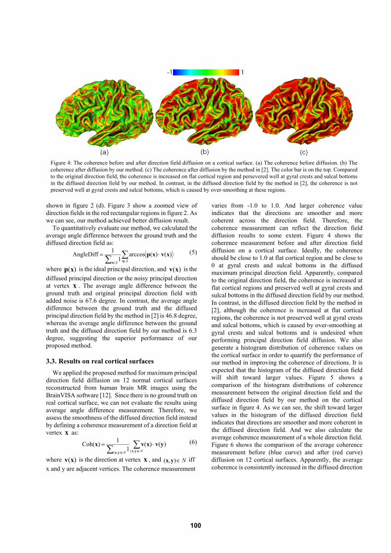
varies from -1.0 to 1.0. And larger coherence value indicates that the directions are smoother and more coherent across the direction field. Therefore, the coherence measurement can reflect the direction field diffusion results to some extent. Figure 4 shows the coherence measurement before and after direction field diffusion on a cortical surface. Ideally, the coherence should be close to 1.0 at flat cortical region and be close to 0 at gyral crests and sulcal bottoms in the diffused maximum principal direction field. Apparently, compared to the original direction field, the coherence is increased at flat cortical regions and preserved well at gyral crests and sulcal bottoms in the diffused direction field by our method. In contrast, in the diffused direction field by the method in [2], although the coherence is increased at flat cortical regions, the coherence is not preserved well at gyral crests and sulcal bottoms, which is caused by over-smoothing at gyral crests and sulcal bottoms and is undesired when performing principal direction field diffusion. We also generate a histogram distribution of coherence values on the cortical surface in order to quantify the performance of our method in improving the coherence of directions. It is expected that the histogram of the diffused direction field will shift toward larger values. Figure 5 shows a comparison of the histogram distributions of coherence measurement between the original direction field and the diffused direction field by our method on the cortical surface in figure 4. As we can see, the shift toward larger values in the histogram of the diffused direction field indicates that directions are smoother and more coherent in the diffused direction field. And we also calculate the average coherence measurement of a whole direction field. Figure 6 shows the comparison of the average coherence measurement before (blue curve) and after (red curve) diffusion on 12 cortical surfaces. Apparently, the average coherence is consistently increased in the diffused direction

Figure 4: The coherence before and after direction field diffusion on a cortical surface. (a) The coherence before diffusion. (b) The coherence after diffusion by our method. (c) The coherence after diffusion by the method in [2]. The color bar is on the top. Compared to the original direction field, the coherence is increased on flat cortical region and persevered well at gyral crests and sulcal bottoms in the diffused direction field by our method. In contrast, in the diffused direction field by the method in [2], the coherence is not preserved well at gyral crests and sulcal bottoms, which is caused by over-smoothing at these regions.

100

fields, suggesting the validity of our proposed method. We also applied the flow field tracking method [2] based

on the diffused maximum principal direction field by our method for sulcal parcellation of these 12 cortical surfaces. In the diffused maximum principal direction field, the directions smoothly flow from gyral crests to sulcal bottoms, therefore, the directions are tracked until reaching sulcal bottoms and all of the vertices flowing to the same sulcal bottom are grouped as a sulcus. For more details of the flow field tracking method, we refer to [2]. The results are shown in figure 7. As we can see, all of the 12 cortical surfaces were consistently parcellated into anatomically meaningful sulci. For example, the central sulci in these 12 subjects, represented by green color, were quite visually reasonable. Each sulcus in each subject was randomly assigned a color, except that the color for the central sulci is interactively identified for visualization purpose. Figure 8 shows a comparison of the parcellation results on a cortical surface based on the diffused direction field by our method and the one by the method in [2]. The dashed yellow circles highlight several regions where the parcellation result

based on the diffused direction field by our method is better.

4. Conclusion In this paper, a novel method for direction field diffusion

on cortical surface is proposed. In this method, the problem of direction field diffusion is formulized as an energy minimization problem, which is converted as a discrete labeling problem and solved efficiently via graph cuts. The method has been validated on both synthesized surfaces and real cortical surfaces, and promising results have been achieved. Our feature work will include further validation of the method on more subjects.

References [1] A.M. Dale, B. Fischl, and M.I. Sereno. Cortical

surface-based analysis: I. Segmentation and surface reconstruction. Neuroimage, 9(2):179-194, 1999.

[2] G. Li, L. Guo, J. Nie, and T. Liu. Automatic cortical sulcal parcellation based on surface principal direction flow field tracking. NeuroImage, 46(4):923-937, 2009.

[3] M. Boucher, A. Evans, and K. Siddiqi. Oriented morphometry of folds on surfaces. In: Proc. Information Processing in Medical Imaging (IPMI), LNCS, 5636, 614-625, 2009.

[4] B. Tang, G. Sapiro, and V. Caselles. Diffusion of general data on non-flat manifolds via harmonic maps theory: the direction diffusion case. International Journal of Computer Vision 36(2):149-161, 2000.

[5] P. Perona. Orientation diffusions. IEEE Trans. Image Processing 7(3):457-467, 1998.

[6] R. Kimmel, and N. Sochen, N. Orientation diffusion or how to comb a porcupine. Journal of Visual Communication and Image Representation 13(1-2):238-248, 2002.

[7] C. Xu, and J.L. Prince. Snakes, shapes, and gradient vector flow. IEEE Trans. Image Proc., 7(3):359-369, 1998.

[8] Y. Boykov, O. Veksler, and R. Zabih. Fast approximate energy minimization via graph cuts. IEEE Trans. PAMI, 23(11): 1222-1239, 2001.

[9] S. Rusinkiewicz. Estimating curvatures and their derivatives on triangle meshes. In: Proc. Symposium on 3D Data Processing, Visualization and Transmission, pp. 486-493, 2004.

[10] V. Kolmogorov, and R. Zabih. What energy functions can be minimized via graph cuts? IEEE Trans. PAMI, 26(2):147-159, 2004.

[11] R. Szeliski, R. Zabih, D. Scharstein, O. Veksler, V. Kolmogorov, A. Agarwala, M. Tappen, and C. Rother. A comparative study of energy minimization methods for Markov random fields with smoothness-based priors. IEEE trans. PAMI 30(6):1068-1080, 2008.

[12] http://brainvisa.info/

Figure 5: A comparison of coherence distribution before and after direction field diffusion by our method on the cortical surface shown in figure 4.

Figure 6: A comparison of average coherence measurementbefore and after direction field diffusion by our method on 12 cortical surfaces.

101

Figure 7: The cortical sulcal parcellation results of 12 cortical surfaces based on the flow field tracking algorithm using the diffuseddirection field by our method. Note that anatomically corresponding sulci in different cases may have different colors, except that the colors of central sulci for which the color is interactively assigned for visualization purpose.

Figure 8: A comparison of cortical sulcal parcellation result on a cortical surface using different diffused direction fields. (a) The results by the diffused direction field by our method. (b) The results by the diffused direction field by the method in [2]. The dashed yellow circles highlight several regions where the parcellation result based on the diffused direction field by our method is better.

102