arXiv:hep-th/0505100v2 6 Jun 2005 Dipole Deformations of N =1 SYM and Supergravity backgrounds with U (1) × U (1) global symmetry Umut G¨ ursoy ∗ 1 and Carlos N´ u˜ nez ∗2 ∗ Center for Theoretical Physics, Massachusetts Institute of Technology Cambridge, MA 02139, USA ABSTRACT We study SL(3,R) deformations of a type IIB background based on D5 branes that is conjectured to be dual to N = 1 SYM. We argue that this deformation of the geometry correspond to turning on a dipole deformation in the field theory on the D5 branes. We give evidence that this deformation only affects the KK-sector of the dual field theory and helps decoupling the KK dynamics from the pure gauge dynamics. Similar deformations of the geometry that is dual to N = 2 SYM are studied. Finally, we also study a deformation that leaves us with a possible candidate for a dual to N = 0 YM theory. MIT-CPT 3630 hep-th/0505100 1 [email protected] 2 [email protected]

Welcome message from author
This document is posted to help you gain knowledge. Please leave a comment to let me know what you think about it! Share it to your friends and learn new things together.
Transcript
arX
iv:h
ep-t
h/05
0510
0v2
6 J
un 2
005
Dipole Deformations of N = 1 SYM and Supergravity
backgrounds with U(1) × U(1) global symmetry
Umut Gursoy ∗1 and Carlos Nunez ∗2
∗ Center for Theoretical Physics, Massachusetts Institute of Technology
Cambridge, MA 02139, USA
ABSTRACT
We study SL(3, R) deformations of a type IIB background based on D5 branes that is
conjectured to be dual to N = 1 SYM. We argue that this deformation of the geometry
correspond to turning on a dipole deformation in the field theory on the D5 branes. We give
evidence that this deformation only affects the KK-sector of the dual field theory and helps
decoupling the KK dynamics from the pure gauge dynamics. Similar deformations of the
geometry that is dual to N = 2 SYM are studied. Finally, we also study a deformation that
leaves us with a possible candidate for a dual to N = 0 YM theory.
MIT-CPT 3630
hep-th/0505100
[email protected]@lns.mit.edu
Contents
1 Introduction 2
1.1 General idea of this paper . . . . . . . . . . . . . . . . . . . . . . . . . . . . 4
2 Warm-up: Transformations of the Flat D5 Brane Solution 7
2.1 The flat D5 brane . . . . . . . . . . . . . . . . . . . . . . . . . . . . . . . . . 7
2.2 The General Transformation . . . . . . . . . . . . . . . . . . . . . . . . . . . 8
2.3 Regularity of Transformed D5 . . . . . . . . . . . . . . . . . . . . . . . . . . 10
2.4 The Gauge Theory . . . . . . . . . . . . . . . . . . . . . . . . . . . . . . . . 12
2.5 Dual of the Dipole Theory . . . . . . . . . . . . . . . . . . . . . . . . . . . . 13
3 N = 1 SYM and the KK-Mixing Problem 14
3.1 Review of the Geometry Dual to N = 1 SYM . . . . . . . . . . . . . . . . . 14
3.2 Dual Field Theory and the Dipole Deformation of the KK Sector . . . . . . 16
4 Deformations of the Singular N = 1 Theory 20
4.1 The Singular Solution a(r)=0 . . . . . . . . . . . . . . . . . . . . . . . . . . 20
4.2 Transformations in the R-symmetry Directions . . . . . . . . . . . . . . . . . 23
4.3 The General β Transformation . . . . . . . . . . . . . . . . . . . . . . . . . . 24
5 Deformation of the Non-singular N = 1 Theory 25
5.1 Confinement . . . . . . . . . . . . . . . . . . . . . . . . . . . . . . . . . . . . 27
5.2 The Beta Function . . . . . . . . . . . . . . . . . . . . . . . . . . . . . . . . 27
5.3 KK Modes and the Domain Wall Tension . . . . . . . . . . . . . . . . . . . . 30
6 PP-waves of the Transformed Solutions 32
6.1 General Properties . . . . . . . . . . . . . . . . . . . . . . . . . . . . . . . . 33
6.2 PP-wave of the Transformed Flat D5 . . . . . . . . . . . . . . . . . . . . . . 34
6.3 PP-wave of the Transformed D5 on S2 . . . . . . . . . . . . . . . . . . . . . 35
6.4 PP-wave Limit of the Transformed Non-singular Solution . . . . . . . . . . . 35
7 Deformations of the N = 2 Theory 37
7.1 Transformation along a non-R-symmetry Direction . . . . . . . . . . . . . . 38
7.2 Transformation along the R-symmetry Directions . . . . . . . . . . . . . . . 40
8 Summary and Conclusions 41
1
9 Acknowledgments 43
A Appendix: Solution Generating Technique 43
B Appendix : The Non-Commutative N = 1 SYM Solution 44
C Appendix: The Non-Commutative KK theory 46
D Appendix: Details on Rotations in R-symmetry Direction 47
E Appendix: Explicit Form of the coordinate transformation in Section 6.4 48
1 Introduction
The AdS/CFT conjecture [1] [2] [3] is one of the most powerful analytic tools for studying
strong coupling effects in gauge theories. There are many examples that go beyond the
initially conjectured duality. First steps in generalizing the original duality to non-conformal
examples were taken in [4]. Later, very interesting developments led to the construction of
the gauge-string duality in phenomenologically more relevant theories i.e. minimally or non-
supersymmetric gauge theories [5]. New geometries that realize various different aspects of
gauge theories allowed us to deepen our knowledge on the duality.
Conceptually, the most clear set up for less symmetric theories is obtained by breaking the
conformality and partial supersymmetry by deforming N = 4 SYM with relevant operators
or VEV’s. The models put forward by Polchinski and Strassler [6] and Klebanov and Strassler
[7] belong to this class. Many authors have contributed to the understanding of this class
of set-ups. The review [8] provides a nice summary of the procedure to compute correlation
functions and various observables.
On the other hand, a different set of models, that are less conventional regarding the UV
completion of the field theory have been developed. The idea here is to start from a set of
Dp-branes (usually with p > 3), that wrap a q-dimensional compact manifold in a way such
that two conditions are satisfied: One imposes that the low energy description of the system
is (p − q) dimensional, that is, the size of the q-manifold is small and is not observable at
low energies. Secondly, it gives technical control over the theory to require that a minimal
amount of SUSY is preserved. For example, the resolution of the the Einstein eqs. is eased.
It turns out that, in this second class of phenomenologically interesting dualities, the UV
completion of the field theory is a higher dimensional field theory.
There are several models that belong to this latter class, and in this paper we are interested
in those that are dual to N = 1 and N = 2 SYM. The model dual to N = 1 SYM [9] builds
on a geometry that was originally found in 4-d gauged supergravity in [10]. The model that
2
is dual to N = 2 SYM was later found in [11]. It must be noted that all of the models in this
category are afflicted by the following problem: they are not dual to “pure” field theory of
interest, but instead, the field theory degrees of freedom are entangled with the KK modes
on the q-manifold in a way that depends on the energy scale of the field theory. The KK
modes enter the theory at an energy scale which is inversely proportional to the size of the
q-manifold and the main problem is that this size is comparable to the scale that one wants
to study non-perturbative phenomena such as confinement, spontaneous breaking of chiral
symmetry, etc. Nevertheless, this limitation can be seen as an artifact of the supergravity
approximation and will hopefully be avoided once the formulations of the string sigma model
on these RR backgrounds becomes available. Many articles have studied different aspects of
these models. Instead of revisiting the main results here, we refer the interested reader to
the review articles [13].
Very recently, an interesting development took place by the paper of Lunin and Malda-
cena [14]. The authors considered a general background of IIB SG 1 that possess two shift
isometries, hence includes a torus as a part of the geometry. This U(1) × U(1) isometry
allows one to generate new SG solutions by performing an SL(2, R) transformation on the
τ parameter of the torus:
τ = B12 + i√
det[g], (1.1)
where the real and imaginary parts are the component of the NS two-form along the torus
and the volume of the torus respectively. This transformation combined with the usual
SL(2, R) symmetry of the IIB theory (that acts on the axion and dilaton) closes onto a
larger group SL(3, R). A two-parameter subgroup of this general symmetry is singled out
by the requirement of regularity in the transformed solutions. This specific subgroup is
referred to as the β-transformation. A natural question from the point of view of the gauge-
gravity duality concerns the dual of the β transformations on the field theory side. In
other words, if we consider a geometry that is associated to a known field theory, what
deformation in the field theory does the transformed solution produce? The answer to this
question that was proposed by Lunin and Maldacena [14] is quite interesting: Associated
with the U(1)×U(1) isometry of the geometry, there are two separate shift transformations
that act on the component fields of the field theory. If we denote the charges of two canonical
fields φ1 and φ2 in the field theory as q1i and q2
i under these transformations, then, the effect
of the β-transformation in the dual field theory can be viewed as modifying the product of
fields in the Lagrangian according to the following rule:
φ1(x)φ2(x) → φ1(x) ∗ φ2(x) = eiπβ det(qji)φ1(x)φ2(x), (1.2)
Therefore this deformation is very much in the spirit of non-commutative deformations of
field theories [15].
1See [14] for discussion also in cases of IIA and 11D SG.
3
The reason behind this result lies in the consideration of associated D-brane picture. One
considers the geometry produced by a number of D-branes. Then the general idea in [14] is
that, depending on the different locations of the torus in the full geometry, one introduces
various different type of β-deformations on the gauge theory that lives on the D-branes. For
example, the choice of the torus in the directions transverse to the D-branes yields a defor-
mation where the two symmetry transformations in (1.2) are two global U(1) symmetries
of the field theory. Lunin and Maldacena gave a specific Leigh-Strassler deformation [16]
of N = 4 SYM as an example of this case. On the other hand, when the torus is along
the D-brane coordinates then the associated deformation of the field theory is precisely the
standard non-commutative deformation of the field theory along the torus directions. In this
case, the two charges in (1.2) are the momenta qix,y = pix,y of φi along the torus. Finally,
another interesting case that we have more to say in this paper is the case where one of the
torus directions is along the branes and the other along one of the transverse directions. In
this case the β-transformation of the original geometry corresponds to the so-called “dipole
deformation” of the field theory [17].
1.1 General idea of this paper
In this work, we consider the N = 1 and N = 2 geometries of [9] and [11] and study
the effects of various β-deformations. From the general arguments of [14] that we repeated
above, we expect that, if one considers a toroidal isometry that is transverse to the field
theory directions, and one makes the β-deformation along these directions, this will modify
only the fields that are charged under these transverse directions. In other words, in the field
theory dual to this particular β-transformed theory, the dynamics of the KK-modes will be
modified, whereas the gauge theory dynamics—that we are ultimately interested in—will
not be affected. Then, one may ask, whether or not the change that one produces in the
KK-sector of the field theory cures the problem of entanglement of these unwanted modes
with the “pure” gauge theory dynamics. In this paper we present evidence that the answer
is in the affirmative. We present our discussion mainly for the case of N = 1 theory, but the
same considerations apply in the case of N = 2.
Specifically, we consider the geometry that is presented in [9] and apply a real β trans-
formation that also keeps the supersymmetry of the theory intact. Then we repeat the
computations of the VEV of Wilson loops, θYM and βYM -function of the theory from the
deformed geometry. We show that these results are independent of the deformation param-
eter. The case of imaginary β deformation is also interesting in that it changes these results,
however we show that in that case the dual geometry is singular, hence the gravity computa-
tions of the field theory quantites cannot be trusted. In order to investigate whether the real
β transformation affects the KK sector of the theory, we compute the masses of a particular
kind of KK modes in the deformed geometry. This computation is done both as a dipole
4
field theory computation and as a supergravity computation. As a field theory calculation
it is easy to show that the particular dipole deformations that we consider when reduced to
4D yield shifts in the KK masses. In the supergravity side, we compute the volume of S3 in
the deformed solution and show that indeed the volume becomes smaller as one turns on β.
Therefore these KK-modes indeed begin to decouple from the pure gauge theory dynamics
when one turns on the deformation parameter. We also consider the pp-wave limits of our
deformed geometries with the same goal in mind. Namely, to analyze the effects of deforma-
tion on the dynamics of the KK-sector. The analysis results in a β correction to the original
pp-wave that was obtained from the original geometry of [9]. Therefore the pp-wave analysis
also confirms the claim that the dynamics of the KK-modes are modified in a non-trivial
way. Similar observations hold for the case of β-deformed N = 2 geometry.
We also consider another interesting geometry that is obtained from the singular “UV”
solution that was found in [9]. The singular solutions dual to minimally supersymmetric
gauge theories are interesting in their own right. Indeed, historically first the singular dual
geometries have been found [12][9] and then the resolution of the singularities have been
discovered [7][9]. The singular solutions generally believed to encode information on the UV
behavior of N = 1 SYM. The singular solution in [9] preserves an additional U(1) symmetry
that is associated with the chiral R-symmetry of the N = 1 SYM in the UV. It is sometimes
denoted as the ψ isometry of the solution. We consider choosing the torus such that one
leg is along the direction of ψ. Then we perform the β transformation to generate new
solutions. As this SL(3, R) transformation does not commute with the R-symmetry the
resulting theory is non-supersymmetric. Therefore by this method, we generate a geometry
that would-be a candidate for a dual of non-supersymmetric pure YM, once the singularity at
r = 0 is resolved. We also observe that in the case of β-transforming along the R-symmetry
direction both the real and imaginary parts of the transformation is allowed: One does
not generate any irregularities that were present in the previous case of supersymmetry
preserving transformation. This may rise some hope that in a particular regime of the
relatively larger parameter space of the theory (now consists of both real and the imaginary
parts of β) one may be able to find a resolution to the singularity at the origin. We leave
this question for future work.
In the next section, we move on to a presentation of the β deformations of [14]. Rather
than repeating the discussion in [14], we introduce the basic idea and the technical aspects of
the method in a simple “warm-up” example: the flat D5 geometry. We stress the discussion
of the irregularities associated with the imaginary β transformations.
Section three reviews the dual of N = 1. We review the geometry and present a detailed
discussion of the mixing between the KK and pure gauge dynamics in the original theory.
Specifically, we review the “twisting” procedure and we make a comparison of confinement
and KK scales. In this section we also present our field theory argument for the change in
the masses of the KK modes. We show that the dipole deformation of the 6D field theory
5
when reduced to 4D indeed realizes the idea of improving the KK entanglement problem.
In section 4, we present the β-transformation of the non-singular solution where the β
transformation is chosen in such a way to preserve supersymmetry. In this section, we also
obtain and discuss the aforementioned non-supersymmetric solution that explicitly breaks
the ψ-isometry of singular N = 1 solution.
The main results of our work are presented in section 5, that is devoted to the discussion
of the β deformation of the non-singular N = 1 geometry. There we introduce the trans-
formed solution and discuss its properties. Finally we compute the field theory observables
of interest. In particular, we show that the expectation value of the Wilson loop, θYM and
the beta function βYM are independent of the deformation parameter and we present the
change in the mass of the KK-modes on S3; we also study domain walls and their tensions.
Section 6 discusses pp-wave limits of some of our solutions. We first make some general
observations about how to perform the pp-wave limits in general β-deformed geometries.
In particular we argue that β should be scaled to zero along with R → ∞. This fact
was already observed in [14]. 2 Then we apply this general method of taking the pp-
waves to three geometries in the following order: The flat β-transformed D5 geometry, the
transformed geometry obtained from the singular geometry of D5 wrapped on S2 and finally
the non-singular β deformed N = 1 geometry.
Section 7 includes our results for the deformations of the N = 2 geometry. We give a
summary and discuss various open directions in our work in the final section 8. Various
appendices contain the details of our computations.
Here is a brief summary of the very recent literature on the subject. After the paper [14]
presented the idea described above, together with some checks, Ref. [18] studied the pro-
posal from the view point of comparing semi-classical strings moving in these backgrounds
with anomalous dimensions of gauge theory operators. Also aspects of integrability of the
spin chain system that is associated with the Leigh-Strassler deformation are studied. Ref.
[19], presented a nice way of understanding (the bosonic NS part of) the SL(3, R) trans-
formations in terms of T dualities; also made a connection with Lax pairs and found new
non-supersymmetric deformations.
A final note on the notation: As we discuss in the next section, we will mainly be concerned
with the real β transformations in this paper —unless specified otherwise— because of the
concerns about irregularity of the imaginary β transformations. These specific real trans-
formations were denoted as γ-transformations in [14]. Therefore the term γ-transformation
will be used instead of β in what follows.
2Note a misprint in [14]: β goes to zero instead of ∞.
6
2 Warm-up: Transformations of the Flat D5 Brane So-
lution
In this section, we outline the solution generating technique in a simple warm-up example.
This allows us to introduce the basic idea and the necessary notation that will be used in
the following sections. More importantly, the examples we discuss here shall serve as an
illustration of when and how the SL(3, R) transformations lead to irregular solutions. The
criteria for regularity of the transformation was outlined in [14] and a specific transformation
of the NS5 (or D5) brane was mentioned as an example of irregular behavior. Here, we discuss
this point in detail.
2.1 The flat D5 brane
Let us consider N D5 branes in flat 10D space-time. The solution in the string frame is,
ds2 = eφ[
dx21,5 + α′gsN(dr2 +
1
4
3∑
i=1
w2i )
]
, F(3) =α′N
4ω1∧w2∧w3, e
φ =α′gs(2π)
3
2√N
er. (2.3)
We define the su(2) left-invariant one forms as,
w1 = cosψdθ + sinψ sin θdϕ ,
w2 = − sinψdθ + cosψ sin θdϕ ,
w3 = dψ + cos θdϕ . (2.4)
Ranges of the three angles are 0 ≤ ϕ < 2π, 0 ≤ θ ≤ π and 0 ≤ ψ < 4π.
One easily sees that this solution includes a torus that is parametrized by ψ and ϕ as part
of its isometries. In order to perform the SL(3, R) transformation that was specified in [14],
one writes (2.3) in the form that separates the torus part from the 8D part that is transverse
to the torus. The 8D part is left invariant (up to an overall factor) under the transformation.
We shall use the notation introduced in [14] in order to avoid confusion (see our Appendix
A for a summary). The D5 metric, (2.3) can be written as,
ds2 =F√∆
(Dϕ1 − CDϕ2)2 + F
√∆(Dϕ2)
2 + gµνdxµdxν . (2.5)
In this particular case, the torus is given by,
Dϕ1 = dψ + A(1), Dϕ2 = dϕ+ A(2). (2.6)
7
The connection one-forms, A(1) and A(2) that are required to put a generic metric in the
above form, vanish in this simple case:
A(1) = A(2) = 0. (2.7)
The 8D part of the metric in (2.3) is,
gµνdxµdxν = dx2
1,5 +N(dr2 +1
4dθ2). (2.8)
We introduced the following metric functions,
F =α′gsN
4eφ sin θ, ∆ = sin2 θ, C = − cos θ. (2.9)
Similarly, one separates the torus and the transverse part in the RR two form in a generic
way as follows [14] and Appendix A:
C2 = C12Dϕ1 ∧Dϕ2 + C(1) ∧Dϕ1 + C(2) ∧Dϕ2 −1
2(A(a) ∧ C(a) − c). (2.10)
C(1) and C(2) are one-forms and c is a two-form on the 8D transverse part. In this particular
example, one can take the RR form as follows:
C2 =α′N
4ψw1 ∧ w2. (2.11)
Then, various objects that appear in the general formula (2.10) become,
C(2) =α′N
4ψ sin θdθ, C12 = C(1) = c = 0. (2.12)
2.2 The General Transformation
Now, we consider the transformation of a general solution of IIB SG under the following
two-parameter subgroup of SL(3, R) 3:
Λ =
1 γ 00 1 00 σ 1
In the next subsection, we work out the details of the transformation in the simple example
of (2.3).
3This specific subgroup - actually a larger one which also includes the ordinary SL(2, R) of IIB in part- was specified in [14] as a necessary condition for the regularity of the transformed geometry. Althoughnecessary, it is not sufficient for the regularity, as we discuss further below.
8
Consider a general solution to IIB Supergravity. Various components of the RR two-form,
NSNS two-form, the four-form and the A-vectors that are defined in (2.5) are grouped into
the following combinations that transform as vectors under SL(3, R) ([14] and Appendix A):
V (i)µ = (−ǫijB(j)
µ , A(i)µ , ǫ
ijC(j)µ ),
Wµν = (cµν , dµν , bµν). (2.13)
Here B(1), B(2), b and d are components of the NS form and the four-form that follows
from the separation of the torus and the transverse part in complete analogy with (2.10)[14].
Their explicit transformation under (2.2) is given as,
(V (i))′ = (−ǫijB(j), A(i) + γǫijB(j) − σǫijC(j), ǫijC(j))
W ′ = (c + γd, d, b+ σd) (2.14)
Transformation of various scalar fields that we defined above is obtained as follows (see
our Appendix A for a summary of these results). One constructs a 3 × 3 matrix, gT , from
the scalar F , the dilaton, and the torus components of the RR and NS forms, C12 and B12.
The components of the initial gT are 4,
gT1,1 = (eφF )−1/3, gT2,2 = e−φ/3F 2/3, gT3,2 = −C12(F )−1/3e2/3φ, gT3,3 = e2/3φ(F )−1/3 (2.15)
and all of the other components are zero.
Now, a few words about how to obtain the transformed matrix: The object that transforms
as a matrix under SL(3, R) is the following one:
M = ggT , M → ΛMΛT . (2.16)
Thus, one can read off the transformation of gT as,
gT → ηTgTΛT , (2.17)
where η is an SO(3) matrix that can be parametrized by three Euler angles. These angles
are determined by demanding that the transformed gT has the specific structure given in
[14], namely its (1, 3), (2, 1) and (2, 3) components vanish. We obtain the new values for
F, eφ, C12, χ, B12 as,
F ′ = FG√H, eφ
′
= eφH√G, B′
12 = γF 2G, χ′ = γJ
H, C ′
12 = −JG (2.18)
where we defined,
H = (1 − C12σ)2 + F 2σ2e−2φ,
G = ((1 − C12σ)2 + F 2σ2e−2φ + γ2F 2)−1, (2.19)
J = σF 2e−2φ − C12(1 − C12σ).4Here, we consider the special case of B12 = 0. The most general case is further discussed in the Appendix
A.
9
Using these transformation properties one obtains the new metric as follows:
ds2 =F ′
√D
(Dϕ′1 − CDϕ′
2)2+ F ′
√D(Dϕ′
2)2 + Ustgµνdx
µdxν . (2.20)
Here Dϕ′i include the transformed A forms, i.e.Dϕ′
i = dϕi + A′(i). The volume ratio that
appears in front of the 8D transverse part is,
Ust =e
2
3(φ′−φ)
(F′
F)
1
3
= H1
2 . (2.21)
where we used (2.18) in the last line. The expression for H in (2.19) tells us the important
fact that the 8D volume ratio is different than 1 only for non-zero σ transformations. In
particular an arbitrary γ transformation (with σ = 0), leaves the 8D volume invariant:
Ust(σ = 0) = 1. (2.22)
To extract useful information about the field theory that is dual to the transformed ge-
ometry, one often needs the analogous expression in the Einstein frame. Making a Weyl
transformation to the Einstein frame, one obtains the following volume ratio of the 8D part
in the Einstein frame:
UE = e−1
2(φ′−φ)Ust = G− 1
4 . (2.23)
This ratio is generally different than one for any transformation.
2.3 Regularity of Transformed D5
Now, let us apply this procedure to the particular solution given in (2.9) and (2.12). From
(2.14) we read off the new values of the A forms, and the vector components of the RR form
as,
A(1)′ = −σC(2) = −σα′N
4ψ sin θdθ, (2.24)
C(2)′ = C(2) = −α′N
4ψ sin θdθ, A(2)′ = C(1)′ = 0
Various scalar fields in the new solution are obtained from (2.18). The new metric is,
using (2.24) in (2.20),
ds2 =F ′
√∆
(
dψ − σα′N
4ψ sin θdθ + cos θdϕ2
)2
+ F ′√
∆dϕ2 + Ustgµνdxµdxν . (2.25)
The particular appearance of ψ above makes the transformed metric irregular. This is
because, ψ originally was defined as a periodic variable with period 4π. However the trans-
formed metric is no longer periodic in ψ. One can easily track the origin of this irregularity:
10
It is coming from the contribution of the σ transformation to the A one-forms in (2.24). In
this case where the torus is chosen in the directions transverse to the D5 brane, the RR two
form has the particular form in (2.12) with a bare dependence on ψ and this bare depen-
dence directly carries on to the metric under the σ transformation. Notice that this irregular
behavior does not happen for a one parameter γ-transformation where one sets σ = 0. In
that case one obtains a new regular solution to IIB SG! (or at least one in which we do not
generate new singularities).
One may wonder if this irregularity is due to our particular choice of (2.11): C2 is defined
only up to a gauge transformation and one can try to use a gauge-equivalent expression
where ψ does not appear in this form. For example a gauge equivalent choice of C2 is given
by,
C2 =α′N
4dψ ∧ w3 =
α′N
4cos θdψ ∧ dϕ. (2.26)
Comparison with the general expression, (2.10) shows that,
C12 =α′N
4cos θ, (2.27)
and the rest of the components in (2.10) vanish. In particular, the vector C(1) vanish and
one does not generate any irregular behavior in the metric, as in (2.25).
However, as described in [14], for the regularity of the full solution, one should also make
sure that the RR two-form in the original solution go to the same integer at various poten-
tially dangerous points where the volume of the torus shrinks to zero size.5 One sees from
(2.3) that these singular points where the volume of the ψ-ϕ torus shrinks to zero are given
by θ = 0 and π. Equation, (2.27) tells us that at these points, C2 goes over to −N and +N ,
respectively. As θ is a periodic variable with period π, a discrete jump of 2N in the flux as
one completes the period is unacceptable and generates an infinite field strength. Thus we
conclude that, in case where the torus is chosen in the transverse directions to the D5 brane,
σ transformation is sick, independently of the gauge choice for C2. This does not happen for
the γ transformation. With a completely analogous argument, one shows that 6 the reverse
phenomena happens in case of the NS5 brane solution. In that case there is a non-trivial B2
form and this time the γ transformation exhibits the same irregular behavior, whereas the
σ transformation is free of irregularity.
Finally, let us recall that the Ricci scalar of the original flat D5 brane (2.3) geometry is
bounded for large values of the radial coordinate, where the dilaton becomes large. The
divergence in the dilaton indicates the need to passing to an S-dual description that is
5In [14], this argument was made for B2 under the γ transformation. Same argument applies to C2 inthe case of σ transformation.
6One can use the formulae given in the previous subsection to work this case out. Our formula (2.18) isapplicable only to the case B12 = 0 (but we wrote general formulas in Appendix A) and one can choose agauge in the NS5 solution such that this happens.
11
given in terms of NS5 branes. At small values of the radial coordinate, the Ricci scalar
diverges instead, thus indicating that we are in the regime where the 6D SYM theory is
the weakly coupled description of the system. In the case of the transformed metric (2.20)
things are more interesting. One can check that, for large values of the radial coordinate,
the transformed dilaton in (2.18) does not diverge (except for the values θ = 0, θ = π) and
the Ricci scalar has an expression that depends on the transformation parameter,
Reff ≈ e−r(−384 + 26η2γ2e2r − η2γ4e4r + η2γ2 cos(2θ)e2r(54 + e2rγ2)
η2(16 + γ2e2r sin2 θ)
)
, η =√
g2YMN(2π)−3,
(2.28)
where η =√
g2YMN(2π)−3. So, if we fix θ as nπ, for large values of the radial coordinate,
we should pass to a dual description. In this case, doing a T-duality seems appropriate.
On the other hand, for values of the angle θ different from nπ we see that the Ricci scalar
(which is non-zero) and the dilaton are bounded for large values of the radial coordinates,
in contrast with the usual D5 case. For this case, it does not seem necessary to pass to a
NS5 description.
For values of the radial coordinate near negative infinity, the Ricci scalar diverges and the
good description is in terms of a 6D gauge theory. The main point of the discussion above
is the fact that the transformed system has in principle a more complicated ‘phase space’
than the original flat D5-branes [4].
2.4 The Gauge Theory
Let us briefly comment on the gauge theory dual of the transformed D5 background. First,
let us recall that the gauge theory on flat D5 branes is a 6D maximally supersymmetric
Yang-Mills theory. The bosonic part of the Lagrangian can be obtained by reducing ten-
dimensional SYM on a four-torus. Schematically, it is given as
S = Tr∫
d6x(
F 2µν + (DµΦ)2 + V ([Φ,Φ])
)
(2.29)
According to the prescription of [14] the new background in (2.20) is dual to (2.29) but
with the potential replaced by a γ deformed one obtained by replacing the products of fields
in V [. . .] by the deformed product of (1.2). We would like to remark that as the torus
of transformation that is formed by ψ and ϕ is transverse to the D5 branes this will only
introduce some phases in the scalar potential.
One should also note that as the transformation that we perform mixes angles that cor-
respond to the SU(2)L × SU(2)R R-symmetry of the 6D SYM theory, this transformation
will break supersymmetry. We shall not dwell on this issue for this warm-up exercise but it
is discussed in more detail for the model of our interest in the next section.
12
2.5 Dual of the Dipole Theory
We would like to end this warm-up section by a discussion of the dipole theories that shall
interest us in the following sections. Our main interest in these exotic quantum theories lies
in the fact that the transformations studied in this section when applied to a supergravity
dual to N = 1 SYM leads to a dipole theory for the KK section of the field theory. This is
discussed in section 3.2 in detail. For the literature on the dipole theories, see [17]. Here we
only summarize some features that will interest us.
A dipole theory is a field theory where the locality is lost due to the fact that some of the
fields come equipped with a “dipolar moment” Lµ such that the product of fields (Φ1,Φ2)
with moments ~L1, ~L2 is given by
Φ1(x)Φ2(x) = Φ1(x− L2/2)Φ2(x+ L1/2) (2.30)
The non-locality of the interaction is manifest. Also, the presence of dipole moments break
Lorentz invariance. We are interested in the particular case where all of the dipole moments
point in the same direction.
If we have a field theory with many fields Φi, each one of them with a global conserved
charge qi, we can pick an arbitrary vector Lµ and the dipole moment of each field is taken
as qiLµ. More generally, if for each field Φi in a collection of n fields, there exist a set of
conserved charges qi1, ...qik, then one can pick an n × k matrix (that we call S) and assign
each field a dipole moment of the form ~L = S~q. In this general case the arbitrary choice of
S, breaks the Lorentz invariance.
The way to construct the dipole Lagrangian is clearly explained in [17]. Basically, the idea
follows the approach of [15], only that in this case, we allow for a non-constant NS field, in
addition to the RR forms. Briefly, the proposal is that, any term in the original Lagrangian
that is of the following form,
Lint = Φ1(x)....Φn(x) (2.31)
is replaced (in momentum space) by
L′int = e
∑n
i<jpiLjΦ1(x)....Φn(x) (2.32)
If we follow the proposal of Lunin and Maldacena [14] that was reviewed above, this is
equivalent to performing an SL(3, R) transformation on a torus that has one direction on
the brane and one external to the brane.
To improve and clarify this discussion, let us now construct the background dual to a
dipole 6D field theory. Once again, we do not worry about preservation of supersymmetry
in this section. If one performs the γ transformation on the torus with one direction along
the D5 brane and one transverse to it, one produces a background dual to a six dimensional
dipole theory as described above. Obviously the Lorentz invariance SO(1, 5) is explicitly
13
broken by the choice of one coordinate along the brane. The background dual to this field
theory is given by
ds2 =F ′
√∆
(dψ + cos θdϕ)2 + F ′√
∆dz2 + Ust(
dx21,4 +
α′gsN(dr2 +1
4(dθ2 + sin θ2dϕ2))
)
(2.33)
where we labeled by z, ψ the directions of the two torus. Following the notation in eq.(2.5),
the functions are defined as
F 2 =α′gsNe
2φ
4, ∆ =
4
α′gsN. F ′ =
F
1 + γ2F 2, A(1) = cos θdϕ,A2 = Ci = C = 0 (2.34)
and Ust is given by (2.21). There is also a dilaton and NS and RR forms that transform
according to eq.(2.18). The original RR two form only has the following component,
c = 2ψα′N sin θdθ ∧ dϕ (2.35)
and it transforms as we indicated in (2.14).
Let us briefly comment on the geometry (2.33). The transformed dilaton is bounded above
for large values of the radial coordinate (and for any values of the angles) unlike the case of
the flat D5 brane analyzed in the previous subsection. The effective curvature is given by,
R ≈ 2e−r(−96 + 8η2γ2e2r + η4γ4e4r
η2(4 + γ2e2r)2
)
, η =√
g2YMN(2π)−3. (2.36)
Again, we find no problem for the large-r regime, neither for the Ricci scalar, nor for the
dilaton. It is peculiar that it is possible to find a value of the radial coordinate where the
Ricci scalar vanishes.
3 N = 1 SYM and the KK-Mixing Problem
3.1 Review of the Geometry Dual to N = 1 SYM
We work with the model presented in [9] (the solution was first found in a 4d context in [10])
and described and studied in more detail in [22]. Let us briefly describe the main points of
this supergravity dual to N = 1 SYM and its UV completion.
Suppose that we start with N D5 branes. The field theory that lives on them is 6D SYM
with 16 supercharges. Then, suppose that we wrap two directions of the D5 branes on a
curved two manifold that can be chosen as a sphere. In order to preserve SUSY a twisting
procedure has to be implemented and actually, there are two ways of doing it. The one we
14
will be interested in this section, deals with a twisting that preserves four supercharges. In
this case the two-cycle mentioned above lives inside a CY3 fold. On the other hand, if the
twist that preserves eight supercharges is performed, the two cycle lives inside a CY2-fold
[11]. This second case will be analyzed in section 7. We note that this supergravity solution
is dual to a four dimensional field theory, only for low energies (small values of the radial
coordinate). Indeed, at high energies, the modes of the gauge theory begins to fluctuate also
on the two-cycle and as the energy is increased further, the theory first becomes N = 1 SYM
in six dimensions and then, blowing-up of the dilaton forces one to S-dualize. Therefore the
UV completion of the model is given by the little string theory.
The supergravity solution that interests us in this section, preserves four supercharges and
has the topology R1,3 × R × S2 × S3. There is a fibration of the two spheres in such a way
that that N = 1 supersymmetry is preserved. By going near r = 0 it can be seen that the
topology is R1,6 ×S3. The full solution and Killing spinors are written in detail in [22]. The
metric in the Einstein frame reads,
ds210 = α′gsNe
φ2
[ 1
α′gsNdx2
1,3 + e2h ( dθ2 + sin2 θdϕ2 ) + dr2 +1
4(wi −Ai)2
]
, (3.37)
where φ is the dilaton. The angles θ ∈ [0, π] and ϕ ∈ [0, 2π) parametrize a two-sphere. This
sphere is fibered in the ten dimensional metric by the one-forms Ai (i = 1, 2, 3). Their are
given in terms of a function a(r) and the angles (θ, ϕ) as follows:
A1 = −a(r)dθ , A2 = a(r) sin θdϕ , A3 = − cos θdϕ . (3.38)
The wi one-forms are defined in (2.4).
The geometry in (3.37) preserves supersymmetry when the functions a(r), h(r) and the
dilaton φ are:
a(r) =2r
sinh 2r,
e2h = r coth 2r − r2
sinh2 2r− 1
4,
e−2φ = e−2φ02eh
sinh 2r, (3.39)
where φ0 is the value of the dilaton at r = 0. Near the origin r = 0 the function e2h behaves
as e2h ∼ r2 and the metric is non-singular. The solution of the type IIB supergravity includes
a RR three-form F(3) that is given by
1
α′NF(3) = −1
4(w1 −A1 ) ∧ (w2 −A2 ) ∧ (w3 − A3 ) +
1
4
∑
a
F a ∧ (wa − Aa ) , (3.40)
15
where F a is the field strength of the su(2) gauge field Aa, defined as:
F a = dAa +1
2ǫabcA
b ∧Ac . (3.41)
Different components of F a read,
F 1 = −a′ dr ∧ dθ , F 2 = a′ sin θdr ∧ dϕ , F 3 = ( 1 − a2 ) sin θdθ ∧ dϕ , (3.42)
where the prime denotes derivative with respect to r. Since dF(3) = 0, one can represent F(3)
in terms of a two-form potential C(2) as F(3) = dC(2). Actually, it is not difficult to verify
that C(2) can be taken as:
C(2)
α′N=
1
4
[
ψ ( sin θdθ ∧ dϕ − sin θdθ ∧ dϕ ) − cos θ cos θdϕ ∧ dϕ −
−a ( dθ ∧ w1 − sin θdϕ ∧ w2 )]
. (3.43)
The equation of motion of F(3) in the Einstein frame is d(
eφ ∗F(3)
)
= 0, where ∗ denotes
Hodge duality. Let us stress that the configuration presented above is non-singular. Finally,
let us mention that the BPS equations also admit a solution in which the function a(r)
vanishes, i.e. in which the one-form Ai has only one non-vanishing component, namely A3.
We will refer to this solution as the abelian N = 1 background. Its explicit form can easily
be obtained by taking the r → ∞ limit of the functions given in eq. (3.39). Notice that,
indeed a(r) → 0 as r → ∞ in eq. (3.39). Neglecting exponentially suppressed terms, one
obtains
e2h = r − 1
4, (a = 0) , (3.44)
while φ can be obtained from the last equation in (3.39). The metric of the abelian back-
ground is singular at r = 1/4 (the position of the singularity can be moved to r = 0 by
a redefinition of the radial coordinate). This IR singularity of the abelian background is
removed in the non-abelian metric by switching on the A1, A2 components of the one-form
(3.38).
3.2 Dual Field Theory and the Dipole Deformation of the KK
Sector
Let us first summarize some aspects of the field theory that is dual to the geometry above.
In [9] this solution was argued to be dual to N = 1 SYM.
The 4D field theory is obtained by reduction of N D5 branes on S2 with a twist that we
explain below. Therefore, as the energy scale of the 4D field theory becomes comparable to
the inverse volume of S2, the KK modes begin to enter the spectrum.
16
To analyze the spectrum in more detail, we briefly review the twisting procedure. In order
to have a supersymmetric theory on a curved manifold like the S2 here, one needs globally
defined spinors. A way to achieve this was introduced in [24]. In our case the argument
goes as follows. As D5 branes wrap the two sphere, the Lorentz symmetry along the branes
decompose as SO(1, 3)×SO(2). There is also an SU(2)L×SU(2)R symmetry that rotates the
transverse coordinates. This symmetry corresponds to the R-symmetry of the supercharges
on the field theory of D5 branes. One can properly define N = 1 supersymmetry on the
curved space that is obtained by wrapping the D5 branes on the two-cycle, by identifying a
U(1) subgroup of either SU(2)L or SU(2)R R-symmetry with the SO(2) of the two-sphere.7
To fix the notation, let us choose the U(1) in SU(2)L. Having done the identification with
SO(2) of the sphere, we denote this twisted U(1) as U(1)T .
After this twisting procedure is performed, the fields in the theory are labeled by the
quantum numbers of SO(1, 3) × U(1)T × SU(2)R. The bosonic fields are,
Aaµ = (4, 0, 1), Φa = (1,±, 1), ξa = (1,±, 2). (3.45)
Respectively they are the gluon, two massive scalars that are coming from the reduction of
the original 6D gauge field on S2, (explicitly from the Aϕ and Aθ components) and finally
four other massive scalars (that originally represented the positions of the D5 branes in the
transverse R4). As a general rule, all the fields that transform under U(1)T—the second
entry in the above charge designation—are massive. For the fermions one has,
λa = (2, 0, 1), (2, 0, 1), Ψa = (2,++, 1), (2,−−, 1), ψa = (2,+, 2), (2,−, 2). (3.46)
These fields are the gluino plus some massive fermions whose U(1)T quantum number is
non-zero. The KK modes in the 4D theory are obtained by the harmonic decomposition
of the massive modes, Φ, ξ,Ψ and ψ that are shown above. Their mass is of the order of
M2KK = (V olS2)−1 ∝ 1
gsα′N. A very important point to notice here is that these KK modes
are charged under U(1)T × U(1)R where the second U(1) is a subgroup of the SU(2)R that
is left untouched in the twisting procedure. On the other hand, the pure gauge fields gluon
and the gluino are not charged under either of the U(1)’s.
The dynamics of these KK modes mixes with the dynamics of confinement in this model
because the strong coupling scale of the theory is of the order of the KK mass. One way
to evade the mixing problem would be to work instead with the full string solution, namely
the world-sheet sigma model on this background (or in the S-dual NS5 background) which
would give us control over the duality to all orders in α′, hence we would be able to decouple
the dynamics of KK-modes from the gauge dynamics. This direction is unfortunately not
yet available.
The dynamics of these KK modes have not been studied in much detail in the literature.
In [20] a very interesting object—the annulon—was introduced. It is composed out of a7The choice of a diagonal U(1) inside SU(2)L × SU(2)R leads to an N = 2 field theory instead, see [11].
17
condensate of many KK modes. More interesting studies on the annulons in this and related
models—some being non-supersymmetric—are in [21].
We would like to argue in this paper that the proposal of Lunin and Maldacena [14] opens
a new path to approach the KK mixing problem in a controlled way. Let us consider the
torus of the β transformations as U(1)T × U(1)R—that is in fact the only torus in the non-
singular solution (3.37) and it is given by shifts along ϕ and ϕ. Then the proposal of LM
implies that,
The β deformation of (3.37) generates a dipole deformation in the dual field the theory,
but only in the KK sector that is the only sector which is charged under U(1)T × U(1)R.
We propose that the deformation does not affect the 4D field theory modes namely the
gluon and the gluino, encouraged by the fact that they are not charged under this symmetry,
as explicitly shown in (3.45) and (3.46).
Let us sketch the general features of this dipole field theory and then present an explicit
argument showing an example of how the dynamics of the KK sector of the theory is affected
under the dipole deformation. In particular, we would like to show that the masses of the
KK modes are shifted under the dipole deformation.
One can schematically write a Lagrangian for these fields as follows:
L = −Tr[14F 2µν+iλDλ−(DµΦi)
2−(Dµξk)2+Ψ(iD−M)Ψ+M2
KK(ξ2k+Φ2
i )+V [ξ,Φ,Ψ]] (3.47)
The potential typically contains the scalar potential for the bosons, Yukawa type interactions
and more. This expression is schematic because of (at least) two reasons. First of all, the
potential presumably contains very complicated interactions involving the KK and massless
fields. Secondly, there is mixing between the infinite tower of spherical harmonics that are
obtained by reduction on S2 and S3. (We were being schematic in the definitions of (3.45)
and (3.46). For example a precise designation for Φ should involve the spherical harmonic
quantum numbers (l,m) on S2.)
Let us now discuss the effect of the β deformation in more detail. The U(1)T corresponds
to shift isometries along ϕ and U(1)R corresponds to shift along ϕ in (3.37). From the D5
brane point of view, the former is a dipole charge and the latter is a global phase on the 6D
fields. Here we only focus on the γ transformation because as we discussed in the previous
section, only the real part of the β deformation gives rise to a regular dual geometry. In
this case, the prescription of Lunin and Maldacena [14] tells us to deform the product of two
fields in the superpotential as follows:
X[~x6]Y [~x6] → eiγ(QX LY −QY LX)X[~x6]Y [~x6], (3.48)
where X and Y are either of the fields that appear in (3.47) and Q and L denotes the charges
of the indicated fields under U(1)R and U(1)T respectively. Note that the action of L on a
field that is charged under U(1)T is a dipole deformation.
18
As a simple exercise, let us investigate the implications of the γ deformation in (3.48) for
the masses of the KK modes. Mass terms in (3.47) are coming from the quadratic terms in the
superpotential. Let us consider the following term in original (undeformed) superpotential,
W ∼MKK Φ+0 [~x6] ξ
++ [~x6] + · · · (3.49)
Here we take two fields of the types in (3.45) with the denoted charges under U(1)T and
U(1)R: Φ has charge +1 under U(1)T and uncharged under U(1)R. ξ carries +1 under both.
Under the deformation (3.48) this term becomes,
W → Wγ ∼MKK eiγ(QΦLξ−QξLΦ) Φ+
0 [~x6] ξ++ [~x6] = MKK e
−iγR3R2LΦ Φ+0 [~x6] ξ
++ [~x6]
≈ MKK Φ+0 [~x6] (1 + γ (R2R3) ∂ϕ) ξ
++ [~x6]. (3.50)
In the last step in (3.50) we used the fact that the dipole generator L corresponds to shifts
in ϕ
Here R2 and R3 are length scales that are associated with the two-cycle and the three-
cycle in the geometry. 8 In general these length scales depend on the radial coordinate
r, hence the charges Q and L will depend on the energy scale of the field theory. In the
far IR region—that we are ultimately interested in—they are both proportional to√α′gsN .
Indeed, we support this claim by our supergravity computations in section 5.3.
Now, consider the spherical decomposition of ξ++ on S2:
ξ++ [~x6] =
∑
l,m
ξ++ [~x4]Yl,m[θ, ϕ]. (3.51)
The spherical harmonics satisfy 9,
− i∂ϕYl,m(θ, ϕ) = mYl,m(θ, ϕ). (3.52)
Then, consider a specific KK mode of ξ++ with the quantum numbers l,m in eq.(3.50).
Expanding (3.50) for small γ and using (3.52) we get the following particular term in the
deformed superpotential,
Wγ ∼MKKΦ+0 [~x6]ξ
++ [~x4; l,m](1 + iγR2R3m). (3.53)
There is a mass term in the scalar potential of the theory that derives from
∣
∣
∣
∣
∂Wγ
∂Φ+0
∣
∣
∣
∣
2
8Note that γ has dimensions of α′−1 therefore in order to make the exponential dimensionless the chargesQ and L should have dimensions of length.
9for a detailed study of the KK modes spectrum see [25]
19
and gives the following mass for this specific KK mode:
(MγKK)2 =
(
1 + (γR2R3m)2)
M2KK . (3.54)
Of course, our computation should be viewed as schematic because in order to obtain the
true mass eigenstates one should diagonalize the mass matrix on infinite dimensional space
of KK harmonics. Nevertheless, it is enough to support our main claim that the dipole
deformation of the N = 1 theory changes the dynamics of the KK modes in a very specific
and controlled way. It is also enough to show that the change in the masses of the KK
modes are always in the positive direction, they increase. We shall verify the mass shift in
(3.54) by explicitly computing the volumes of the two and three cycles in the IR geometry
in section 5.3. There we obtain analytical expressions—as functions of γ— for volume ratios
of deformed over undeformed theories for the S2 and S3 cycles. It is encouraging to see
that the mass ratio is greater than one. This fact is quite tempting to believe that the β
deformation of [9] is a positive step in curing the main problem associated with this model
and similar ones, namely mixing with the KK modes. Our computations therefore suggest
that for large values of γ, one may be able to decouple the KK modes from the IR dynamics;
but the value of γ is to be restricted from above by the condition of small Ricci scalar that is
necessary for the validity of supergravity approximation. Therefore we seem to have a finite
window for the γ parameter where we can make an improvement of the model by pushing
the KK modes up.
Taking very large values of γ might conflict with having a bounded Ricci scalar to stay in
the Supergravity approximation.
Another encouraging fact is directly seen when one considers applying the deformation in
(3.48) in case either of X or Y is the vector multiplet. As the vector multiplet is uncharged
under either of the Q or L we see that the γ transformation of the the N = 1 theory indeed
does not affect the pure gauge dynamics. It acts on the gauge and KK sectors of the theory
(but it may translate into the massless sector through interaction terms). Motivated by the
mass calculation that we presented above, one can consider more elaborate computations
regarding the interaction terms in the potential in (3.47). An interesting question to ask is
how is the IR theory “renormalized” under the γ transformations.
4 Deformations of the Singular N = 1 Theory
4.1 The Singular Solution a(r)=0
In order to apply the SL(2, R) transformation we shall put the metric in (3.37) in the form
explained in [14] (See also Appendix A in this paper). Like before, we will stick with the
definitions given in this paper to avoid confusion. It is very useful to first consider the
transformation of the simpler but singular case of a(r) = 0. This provides us with some
20
intuition and physical insight. The metric of eq.(3.37), written in string frame, in the case
a(r) set to zero reads as follows:
ds2 = F
(
1√∆
(dϕ− Cdϕ+ A(1) − CA(2))2 +√
∆(dϕ+ A(2))2
)
+e2/3φ
F 1/3gµνdx
µdxν (4.55)
where we write the eight dimensional part of the metric that is transverse to the torus as,
gµνdxµdxν = e−2/3φF 1/3[Ddψ2 + eφ(dx2
1,3 + gsNα′(e2hdθ2 + dr2 +
1
4dθ2))], (4.56)
we have defined the following vectors,
A(1) = αdψ, A(2) = βdψ, (4.57)
and the functions F,D,∆, C, α, β that appear above are:
F =α′gsNe
φ
4(4e2h sin2 θ + cos2 θ sin2 θ)
1
2 , ∆ =4e2h sin2 θ + sin2 θ cos2 θ
(4e2h sin2 θ + cos2 θ)2,
C = − cos θ cos θ
4e2h sin2 θ + cos2 θ,D =
α′gsNe2h+φ sin2 θ sin2 θ
4e2h sin2 θ + sin2 θ cos2 θ,
α =cos θ sin2 θ
cos2 θ sin2 θ + 4e2h sin2 θ, β =
4e2h sin2 θcosθ
4e2h sin2 θ + cos2 θ sin2 θ(4.58)
The RR two form given in (3.43) for a(r) = 0 can be written as,
C2 = C12(dϕ+ A(1)) ∧ (dϕ+ A(2)) + C(1)µ (dϕ+ A(1)) ∧ dxµ + C(2)
µ (dϕ+ A(2)) ∧ dxµ
−1
2(A(a)
µ C(a)ν − cµν)dx
µ ∧ dxν . (4.59)
Here various components and one-forms read as follows:
C12 = −1
4cos θ cos θ, C(1) = −C12βdψ − ψ
4sin θdθ, C(2) = C12αdψ +
ψ
4sin θdθ,
c2 =ψ
4(α sin θdψ ∧ dθ + β sin θdθ ∧ dψ) (4.60)
Like in the previous section, various components of the two-form and the A-vectors above
are grouped in combinations that transform under SL(2, R) as vectors:
V (i)µ = (−ǫijB(j)
µ , A(i)µ , ǫ
ijC(j)µ ) = (0, A(i)
µ , ǫijC(j)
µ ), Wµν = (cµν , dµν , bµν) = (cµν , 0, 0) (4.61)
that transform explicitly as,
(V (i))′ = (−ǫijB(j), A(i) + γǫijB(j) − σǫijC(j), ǫijC(j)) W ′ = (c+ γd, d, b+ σd)(4.62)
21
We will concentrate on the γ-transformation. In this case, the vectors and tensors in (2.14)
transform as (V (i))′ = (0, A(i), ǫijC(j)), W ′ = (c, 0, 0). Notice that due to the transforma-
tions above, the differentials Dϕ,Dϕ do not change under SL(3, R). Following what we
explained in the previous section, we can transform the functions appearing in (4.55). We
obtain the new values for F, eφ, C12, χ, B12 as given by eq.(2.18). For the D5 branes, the
γ-transformation leads to nonsingular spaces according to the discussion of the previous sec-
tion, we will concentrate in the following on transformations that have σ = 0. Then the new
fields become,
F ′ =F
(F 2γ2 + 1), B′
12 =F 2γ
(F 2γ2 + 1), e2φ
′
=e2φ
(F 2γ2 + 1), χ′ = γC12, C
′12 =
C12
(F 2γ2 + 1).
(4.63)
Putting all of the things together, we can get the new configuration, that consists in this
case of metric, dilaton, axion, RR and NS two forms and four form. The new metric, in
string frame is given by,
ds2 =F ′
√∆
(Dϕ− CDϕ)2 + F ′√
∆(Dϕ)2 + (e2φ
′
F ′e−2φF )1/3[Ddψ2 +
eφ(dx21,3 + α′gsN(e2hdθ2 + dr2 +
1
4dθ2))] (4.64)
the NS gauge field is Bϕ,ϕ = B′12Dϕ
′ ∧Dϕ′, with B′12 given in (4.63). The new dilaton and
axion are e2φ′
= e2φ
(1+γ2F 2), χ′ = −γ
4cos θ cos θ, the new RR two-form,
C(2)′ = C ′12Dϕ ∧Dϕ− C(1) ∧Dϕ− C(2) ∧Dϕ− 1
2(A(1) ∧ C(1) + A(2) ∧ C(2) − c), (4.65)
with C ′12 given in (4.63). Finally, the RR four form is given by
(C4)′ = −1
2B′
12(c− (A(1) ∧ C(1) + A(2) ∧ C(2))) ∧Dϕ ∧Dϕ. (4.66)
For completeness, let us write here the expressions for the gauge field strengths H ′3, F
′3, F
′5
H ′3 = dB′
12 ∧ (dϕ ∧ dϕ+ αdψ ∧ dϕ+ βdϕ ∧ dψ) +B′12(dϕ ∧ dα+ dβ ∧ dϕ) ∧ dψ (4.67)
F ′3 = dC2 − χ′H ′
3 =
1
4dψ ∧ (sin θdθ ∧ dϕ− sin θdθ ∧ dϕ) + dϕ ∧ dϕ ∧
( 1
1 + γ2F 2dC12 + C12d(
1 − γ2F 2
1 + γ2F 2))
+
(−αdϕ+ βdϕ) ∧ dψ ∧ γ2F 2
1 + γ2F 2dC12 (4.68)
and the RR four form that reads
− 2C ′4 = B′
12(c−A(i) ∧ C(i)) ∧Dϕ ∧Dϕ (4.69)
22
and finally
F ′5 = dC ′
4 − C ′2 ∧H ′
3 (4.70)
What can we learn from this transformed background? One first thing that comes to mind
is related to chiral symmetry breaking. Indeed, as shown in [26], it is enough to work with
the singular background and the respective RR fields to see explicitly the phenomena of χSB
as a Higgs mechanism for a gauge field used to gauge the isometry corresponding to chiral
symmetry (translations in the angle ψ in this case). It should be interesting to do again
this computation in this transformed background. The new ingredients to take into account
are the new NS and RR fields as shown above. We believe that the anomaly will be the
same because, as an anomaly, it can only be affected by the mass less fields. In our case,
the transformed background only takes into account changes in the dynamics of the massive
KK modes. It should be interesting to see this argument working explicitly.
4.2 Transformations in the R-symmetry Directions
In the previous section, we performed rotations that commuted with the R symmetry of
the field theory. Indeed, the R-symmetry of N=1 SYM is represented in the background
studied in in the previous subsection by changes in the angle ψ. The rotations done above,
preserve SUSY, since they do not involve the angle ψ. In this section, we will concentrate
on rotations taking the torus, to be composed of ψ, ϕ; this will break SUSY. Notice that in
this case, the dual field theory to the transformed solution will not be a dipole theory, but
a theory where phases has been added to the interaction terms. Also, notice that we can do
this in the singular solution only, because in the desingularized solution, we do not have the
invariance ψ → ψ + ǫ.
So, to remind the reader, let us write explicitly the 10 metric (3.37) in the singular case
(string frame is used)
ds210 = α′gsNe
φ[ 1
α′gsNdx2
1,3 + e2h ( dθ2 + sin2 θdϕ2 ) + dr2 +
1
4(dθ2 + sin2 θdϕ2 + (dψ + cos θdϕ+ cos θdϕ)2)
]
, (4.71)
We notice that this metric is already written in the form that we want it. Indeed, comparing
we can see that
F =α′gsN
4eφ sin θ, ∆ = sin2 θ, Dϕ1 = Dψ = dψ+cos θdϕ, Dϕ2 = Dϕ = dϕ, C = − cos θ.
(4.72)
and
gµνdxµdxν = e−2φ/3F 1/3[α′gsNe
φ(1
α′gsNdx2
1,3 + e2h ( dθ2 +sin2 θdϕ2 ) + dr2 +dθ2
4)] (4.73)
23
After doing some computations, see Appendix D, we can see that the transformed string
metric reads,
(ds2string)
′ = e2(φ′−φ)/3(
F
F ′)1/3α′gsNe
φ[ 1
α′gsNdx2
1,3 + e2h ( dθ2 + sin2 θdϕ2 ) + dr2
+1
4dθ2
]
+ (F ′√
∆(Dϕ)2 +F ′
√∆
(Dψ + cos θDϕ)2) (4.74)
The new RR and NS fields are explicitly written in the Appendix D. The reader can check
that there is no five form generated. Indeed, there is no C4 generated by the SL(3,R) rotation
and besides the term C2 ∧H3 does not contribute.
This new solution is expected to be non-SUSY, and an occasional resolution of the sin-
gularity at r = 0 could give a dual to YM theory. One might think about, for example, a
resolution by turning on a black hole, dual to YM at finite temperature. This should be very
interesting to solve.
Like in the examples of the D5 brane, doing this transformation is changing quantities like
for example the Ricci scalar, but the place where α′Reff diverges (r → 0 with a divergence
of the form α′Reff ≈ r−7/4) are the same before and after the transformation. The divergent
structure does not seem to become worst by the effect of the gamma transformation.
4.3 The General β Transformation
Transformations of the singular solution i.e.(3.37) for a = 0 where the torus is chosen
transverse to the D5 brane have the interesting property of being regular both for real and
imaginary parts of β. Therefore it is tempting to perform the general β = γ + iσ trans-
formation. Here we, show the regularity of the general transformed solution explicitly, by
presenting the resulting geometry.
The only new feature that one introduces to the results of section 4.2 is that, turning on
σ changes the connections A(i) according to (2.14). The transformed connections are:
A(1)′ = A(1) = cos θdϕ, A(2)′ = A(2) + σC(1) =α′N
4σ cos θϕ, (4.75)
Details are given in Appendix D. Using (2.18), we find the the string frame metric as,
ds2string = Ustα
′gsNeφ[ 1
α′gsNdx2
1,3 + e2h( dθ2 + sin2 θdϕ2) + dr2 +1
4dθ2
]
(4.76)
+F ′√
∆(dϕ+ σα′N
4cos θdϕ)2 +
F ′
√∆
(dψ + cos θdϕ+ cos θdϕ+ σα′N
4cos θ cos θdϕ)2)
(4.77)
Here the new metric functions are given by (2.18) and (2.21) and they generally depend on
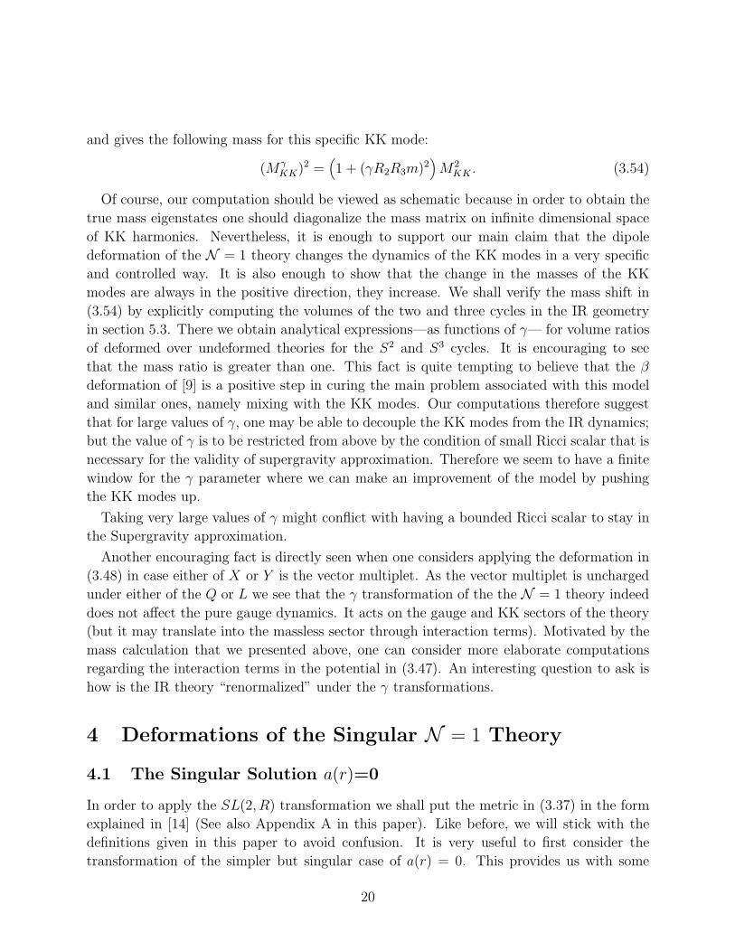
both γ and σ. Eqs. (2.18) also determine how the RR two-form and the dilaton transforms
and shows the new fields that are generated by the general transformation.
24
It should be interesting to study the fate of the symmetry ψ → ψ + ǫ after this transfor-
mation. This symmetry, in the case of N = 1 SYM was associated with chiral rotations [26].
In this case, our theory does not have massless fermions. So, the symmetry corresponds to
some kind of flavor symmetry within the KK sector. It should be interesting to see if this
symmetry gets by the broken and the way studied in [26].
Now that we gained some insight with this type of configurations, let us study the U(1)×U(1) transformation in the case of the non-singular background.
5 Deformation of the Non-singular N = 1 Theory
Now, let us discuss the non-singular case, a(r) 6= 0. The type of problems we have in
mind that might be tackled, are related to previous computations of non-perturbative field
theory aspects from a supergravity perspective. Indeed, in some cases, it was not clear if
the result of this computation was afflicted by the presence of the massive KK modes. So,
finding the transformed background and re-doing the computations with it, might help us
improve this situation, since as we remarked above, both backgrounds do differ in the fact
that their dual theories have different dynamics for the KK modes, results that depend on
the transformation parameter γ will indicate the presence of effects of the KK modes.
We first write the full metric in (3.37) in the following appropriate form for the SL(3, R)
rotation in which the torus and the transverse parts have been separated as follows:
ds2string = eφ[dx2
1,3 + α′gsNdr2] +D1dψ
2 +D2dθ2 +D3dθ
2 + E1dθdθ +
E2dθdψ + E3dθdψ +F√∆
[dϕ+ (α1 − Cβ1)dθ + (α2 − Cβ2)dθ + (α3 − Cβ3)dψ − Cdϕ]2 +
F√
∆(dϕ+ β1dθ + β2dθ + β3dψ)2 (5.78)
To simplify the notation let us define,
f = 4e2h sin2 θ + cos2 θ + a2 sin2 θ, g = a sin θ sin θ cosψ − cos θ cos θ. (5.79)
Then, various functions in (5.78) are given as,
F =α′gsNe
φ
4
√
f − g2, ∆ =f − g2
f 2, C =
g
f,
β1 =f
f − g2a sinψ sin θ, β2 =
g
f − g2a sinψ sin θ, β3 =
f cos θ + g cos θ
f − g2
α1 =a sin θ sinψg
f − g2, α2 =
a sin θ sinψ
f − g2, α3 =
cos θ + g cos θ
f − g2
25
D1 =α′gsNe
φ
4(f − g2)(f sin2 θ − g2 − cos2 θ − 2g cos θ cos θ),
D2 =α′gsNe
φ
4(a2 + 4e2h − f
f − g2a2 sin2 ψ sin2 θ) (5.80)
D3 =α′gsNe
φ
4(1 − a2 sin2 θ sin2 ψ
f − g2), E1 =
a
2α′gsNe
φ(cosψ − g
f − g2a sin2 ψ sin θ sin θ)
E2 = −α′gsNe
φa
2
sinψ sin θ(f cos θ + g cos θ)
f − g2, E3 = −α
′gsNeφ
2
a sin θ sinψ
f − g2(cos θ + g cos θ).
Now, let us focus on the RR two form. Like before, it is useful to define four one forms as
A(i), C(i), i = 1, 2
A(1) = α1dθ + α2dθ + α3dψ, A(2) = β1dθ + β1dθ + β3dψ, (5.81)
and
C(1) = C(1)θ dθ + C
(1)
θdθ + C
(1)ψ dψ, C(2) = C
(2)θ dθ + C
(2)
θdθ + C
(2)ψ dψ, (5.82)
and the two form cµνdxµ ∧ dxν , with components cθθ, cθψ, and all others being zero. In order
to reproduce the RR two-form potential given in (3.43) in the following form,
C(2) = C12Dϕ ∧Dϕ− C(1) ∧Dϕ− C(2) ∧Dϕ− 1
2(A(1) ∧ C(1) + A(2) ∧ C(2) − c); (5.83)
the quantities defined above are determined as,
C12 =1
4(a(r) sin θ sin θ cosψ − cos θ cos θ),
C(1) = (−ψ4
sin θ − C12β1)dθ − (1
4a(r) sin θ sinψ + C12β2)dθ − β3C12dψ,
C(2) = (1
4a(r) sin θ sinψ + C12α1)dθ + (
ψ
4sin θ − C12α2)dθ + α3C12dψ,
c = cθθdθ ∧ dθ + cθψdθ ∧ dψ + cθψdθ ∧ dψ (5.84)
with
cθθ = α1α2 + β1β2 + C12(α1β2 − α1β2) −1
4ψ sin θβ1 +
1
4a sin θ sinψα1
−1
4a cosψ +
1
4aβ2 sinψ sin θ,
cθψ = α1α3 + β1β3 − C12(α1β3 − α3β1) −1
4ψ sin θα3 +
1
4a sinψ sin θβ3,
cθψ = α2α3 + β2β3 − C12(α2β3 − α3β2) +1
4ψ sin θβ3 −
1
4a sinψ sin θα3. (5.85)
One can check that in the limit a(r) → 0 one recovers the result in (4.55).
26
So, after the SL(3, R) rotation we obtain a metric that reads
(ds2string)
′ = (e2(φ
′−φ)F
F ′)1/3
(
eφ[dx21,3 + α′gsNdr
2] +D1dψ2 +D2dθ
2 +D3dθ2 + E1dθdθ +
E2dθdψ + E3dθdψ)
+F ′
√∆
[dϕ+ (α1 − Cβ1)dθ + (α2 − Cβ2)dθ + (α3 − Cβ3)dψ − Cdϕ]2
+F ′√
∆(dϕ+ β1dθ + β2dθ + β3dψ)2 (5.86)
The RR and NS fields will transform according to the rules discussed in previous sections.
Notice that as happened before, the γ transformation leaves the one forms A(i), C(i) invari-
ant. This is a good point to notice that the torus given by the cycle of constant θ, θ, ψ, r, x,
has volume VT2 = F ′ = F1+γ2F 2 after the transformation and that only vanished if F vanishes
or becomes infinite. So, if the original geometry is nonsingular, the transformed one also
is. In the points where the volume of the torus shrinks, it happens that it does in a way
B′12 = Re[τ ] → 0 when
√g′ = Im[τ ] → 0, thus the metric satisfies the criteria in [14] for
nonsingularities.
5.1 Confinement
The first check that this new solution should pass is the confinement. As clearly explained for
example in [27], the expectation value of the Wilson loop can be computed by calculating the
Nambu-Goto action for a string that is connected to a probe brane at infinity and explores
the IR region (r=0) of the background. The criteria for confinement is that if the following
combination (that can be intuitively associated with the tension of the confining string)
Ts =√gttgxx
∣
∣
∣
∣
r=0(5.87)
is non-vanishing then there is linear confinement. The “QCD string” tension, Ts defined
above, is non vanishing. In the original background, the value of Ts = eφ(0). After the
transformation, we can see that the string tension is given by
T ′s =
√
g′ttg′xx = Ust√gttgxx = Ts (5.88)
where Ust is defined in (2.21). We note that the tension would change if we perform a σ-
transformation. It should be interesting to understand the effects of the sigma transformation
in more detail, since they seem to alter important aspects of the gauge theory.
5.2 The Beta Function
Let us compute the beta function, following the lines of [28], [29]. We first revise their steps
and add some comments that might make the derivation more clear. In order to compute
27
beta functions, one needs to define a SUSY cycle where to wrap a D5 brane at finite distance
from the origin. It was found in [22] that such cycle exists for an infinite value of the radial
constant. The cycle is given by the following identifications 10
θ = θ, ϕ = 2π − ϕ, ψ = π, 3π (5.89)
Notice that, since this is a calibrated (SUSY) cycle for large values of the radial coordinate, we
should be considering the “abelian version” (a(r) = 0) of the background. We proceed with
the full nonsingular solution, but one should keep in mind that this is a good approximation
only for r → ∞. Then, one needs to introduce a relation between the radial coordinate
r, and the energy scale of the theory. We will take the following relation [30], [28], that
identifies the gaugino condensate with the function a(r).
a(r) =Λ3
µ3= 〈λλ〉 (5.90)
This relation has an intuitive explanation since the gaugino condensate, like the turning-
on of the function a(r) are phenomena that occur in the IR, that is at small values of
the energy/radial coordinate. This identification (5.90), is indeed the reason for doing the
calculation in the non-singular background, even when the cycle we use is supersymmetric
only for large values of r.
Using (5.89) one defines the coupling constant as
1
g2YM
=1
(2π)2gsα′
∫ 2π
0dϕ
∫ π
0dθe−φ(gxx)2
√
detG6. (5.91)
This gives,π2
4g2YMN
= (4e2h + (a(r)2 − 1)2) (5.92)
Therefore on obtains the beta function as
β =dgYM
dlog(µ/Λ)= −g
3YMN
8π2
d( π4g2N
)
dr(d(−1/3Log(µ/Λ))
dr)−1. (5.93)
Expanding the result for large values of the radial coordinate and using an expansion for
large r of (5.92) one gets,
β = −3g3YMN
8π
1
(1 − g2YM
N
8π)
(5.94)
If one keeps higher orders in the r expansion, one gets extra terms that in [28] were attributed
to fractional instantons.
10notice that also the cycle θ = π − θ, ϕ = ϕ, ψ = 0, 2π is SUSY at large values of r
28
The reader may wonder what is the origin of these extra effects. On one hand, one might
think that they are a pure N = 1 SYM effects. Or might argue that they are an effects due
to the KK modes of the field theory to which this supergravity solution is dual. Apart from
these two possibilities, one can think that they are spurious effects coming from the fact that
for small values of r in the expansion of the quantities above, the supersymmetry is broken,
since the cycle (5.89) is no longer SUSY.
In order to discard some of these alternatives, we compute the beta function in the γ
deformed non-singular background. If these extra terms that seem to modify the original
NSVZ result are effects of the KK modes, then by our general philosophy in this paper, the
beta function should be different in the deformed theory.
Let us take the same cycle in the transformed solution (5.86) 11 The relevant six dimen-
sional part of the metric is
(ds26D)′ = [eφ(dx2
1,3 + gsNα′dr2) + (D2 +D3 + E1)dθ
2] +
F ′
√∆
((1 + C)dϕ+ (α2 − Cβ2)dθ)2 + F ′
√∆)(−dϕ+ (β1 + β2)dθ)
2 (5.95)
We note that at the special cycle the metric components reduce to the original undeformed
components except than the change from F to F ′. This gives a factor of F ′/F which exactly
cancels out the change in the dilaton in (5.91). So, computing the determinant and defining
the coupling as before,
1
g2YM
=1
(2π)2gsα′
∫ 2π
0dϕ
∫ π
0dθe−φ
′
(g′xx)2√
detG6. (5.96)
Using the fact that
eφ−φ′
= (1 + γ2F 2)1/2 (5.97)
the coupling readsπ2
4g2YMN
= [4e2h + (a2 − 1)2]. (5.98)
This is precisely the same as (5.92). Then, one repeats the procedure in eq. (5.93) [28], [29]
and obtains the same result for the beta function in the deformed theory.
One can repeat the same computation for the theta parameter of Yang-Mills. The essen-
tials of the computation do not change. θYM is the same as in the undeformed theory.
We learn that the computation for beta function seems robust under the deformations.
Indeed, the beta function is a field theory result, that should be independent of the KK
modes dynamics. So, this transformed solution that only changes the KK sector of the dual
field theory, does not produce any effect in the result (5.93). On the other hand, the fact
11We believe that by general properties of the γ transformation this cycle is also supersymmetric in thedeformed geometry. It should be interesting to verify this by an explicit BPS calculation.
29
that we got the same result is perhaps indicating that the result should only be taken to
first order in the large r expansion thus implying that there are no “fractional instanton”
corrections. Or may be, the “fractional instantons” are a genuine field theory effects; but
the result of these computations above, make sure that the KK modes have no relation to
them whatsoever. Finally, we note that it should of course be of great interest to find the
SUSY cycle that computes the beta function in the IR.
5.3 KK Modes and the Domain Wall Tension
There are two types of KK modes, those that are proportional to the volume of an S2 in
the geometry and those that are proportional to the volume of a three cycle, the first type
are the ‘gauge’ KK modes. On the other hand, the volume of the non-vanishing three cycle
at the IR (at r = 0) is inversely related to the masses of the “geometric” KK modes in the
theory. Therefore it is very interesting to see whether or not these volumes are changed by
the transformation. If the volume decreases under the transformation, it would be a non-
trivial improvement of the model as the undesired KK degrees of freedom would have better
decoupling. Let us start with the ‘geometric’ KK modes. The three cycle in the original
theory is given by,
θ = ϕ = r = ~x = 0. (5.99)
In the original metric (3.37), this volume is, (in the string frame),
V = 2π2(α′gsNeφ(0))
3
2 . (5.100)
Now, we consider the same cycle in the transformed geometry (5.86). Using eqs. (5.81) the
reader can see that one obtains
V ol(S3′) = π2(α′gsNeφ0)3/2
∫ π
0dθ
sin θ
1 + µ2 sin2 θ
= π2(α′gsNeφ0)3/2(
2arctanh(µ/√
1 + µ2)
µ√
1 + µ2)
∝ π2(α′gsNeφ0)3/2(2 − 4
3µ2 + ..),
where 16µ2 = γ2(α′gsNeφ0)2. It is useful to consider the ratio,
(
M ′KK
MKK
)2
=
(
V olS3
V olS3′
)2/3
=
(
µ√
1 + µ2
2arctanh[µ/√
1 + µ2]
)2/3
. (5.101)
So, we see that the mass of these ‘geometric’ KK modes indeed increase improving the
decoupling between the KK and the pure SYM sector.
30
Now, let us analyze the mass of the ‘gauge’ KK modes, that are inversely proportional to
the volume of some S2 defined in the geometry. Let us define the two cycle as,
θ = ϕ = ψ = x = r = 0, (θ, ϕ) (5.102)
Computing the line element of this two cycle one gets (once again, we concentrate on the γ
transformation)
ds2 = (D2 + β21F
′√
∆)dθ2 +F ′
√∆dϕ2 (5.103)
so, the volume of this two cycle near r = 0 is
V ol(S2′) =πα′gsNe
φ0
2
∫ π
0
dθ√
1 + 116
(γα′gsNeφ0 sin θ)2→
V ol(S2′) ≈ πα′gsNeφ0
2(1 − γ2α′(gsN)2e2φ0
64) (5.104)
again, it is convenient to present the quotient,
(m′kk
mkk)2 = (
∫ π
0
dθ√
1 + 116
(γα′gsNeφ0 sin θ)2)−1 ≈ 1 +
1
16(γα′gsNe
φ0)2 (5.105)
So, we see that the mass of the ‘gauge’ KK modes also increases when this transformation
is performed. We would like to stress again that under the σ transformation, the volumes
above indeed change. However, as the σ transformation produces irregularities, the role of
the σ modification of the original model is unclear 12
Another interesting quantity to compute is the tension of a Domain Wall. A domain wall
is thought as a D5 brane that wraps the three cycle (5.99) and extends in (2 + 1) directions
of spacetime. The way of computing the tension of this wall is by computing the coefficient
in front of the Born-Infeld action for a D5 as indicated above.
Swall =∫
d3x(∫
dΩ3e−φ′√
detG6) + CS (5.106)
from the term in parentheses we read the tension of the domain wall, to be
Twall =∫ 4π
0
∫ 2π
0
∫ π
0dθdϕdψe−φ
′+2φ(e2(φ′−φ) F
F ′α′gsN)1/2 F
(1 + γ2F 2)
∣
∣
∣
∣
r=0(5.107)
Using (5.97) we see that the result changes and the chane is explicitly given as,
T ′
T=
1
2+
1
πarctan(
4e−φ0
γα′gsN). (5.108)
12We are grateful to Juan Maldacena for suggesting that redefinitions of the periodicities of the originalcycles may improve the situation.
31
One should perhaps interpret this as an effect of the KK modes in field theory observables
because the cycle we are choosing (5.99) is not the appropriate one for computing domain
walls. This point deserves more study.
In this line, it would be nice to analyze what happens to the computation of baryonic
strings as D3 branes wrapping the previous 3 cycle done in the paper [31].
The result of the last two subsections is basically that under the γ transformations many
field theory aspects of N=1 SYM are not changed when computed from the transformed
background, while the KK modes change their masses. This, on one hand is reassuring of
the conjectured duality, because as we stressed many times, the transformed background
only differs in the dynamics of the KK modes. It is of interest to see an example where
some changes in the dynamics are indeed expected to happen. This example is provided by
pp-waves. The objects called annulons and studied in [20], [21] are constructed to be heavy
composites of many KK modes (this composite is called ‘hadron’ in the papers mentioned
above). These objects are studied in a plane wave approximations of the geometry. So, in
order to see real changes in dynamics of KK modes, in the next section,we will study these
composites in the transformed backgrounds.
6 PP-waves of the Transformed Solutions
PP-wave limits of various transformed solutions are quite interesting. The first example of
this kind was discussed by Lunin and Maldacena [14] where they considered a particular
PP-wave limit of the β transformed AdS5 × S5 geometry; it is quite amusing to observe
that with different arguments and objectives Niarchos and Prezas found the same plane
wave some years ago [23]. In most cases, one can indeed obtain PP-waves that lead to
quantizable string actions. Here, we would like to first make some observations about the
general properties that are satisfied by the PP-waves of the transformed geometries. Then,
we exemplify these properties by studying two simple cases, those of flat the D5 brane and
singular D5 wrapped on S2. Finally we discuss the PP-wave associated to the transformed
non-singular geometry that we obtained in section 4.2.
We restrict our attention to the pp-wave limits that are obtained by the scaling of the
same coordinates, before and after the transformation. The motivation for this is to study
the effects of the SL(3, R) transformation to the pp-wave limits. In general one may also ask
whether or not the transformed geometry admits interesting pp-wave limits other than the
pp-waves of the original geometry. A separate issue is to apply the SL(3, R) transformation
to the pp-wave itself and seek for new quantizable geometries. We note that generally the
pp-wave limit does not commute with the SL(3, R) transformation. We do not investigate
these interesting issues further in this paper.
32
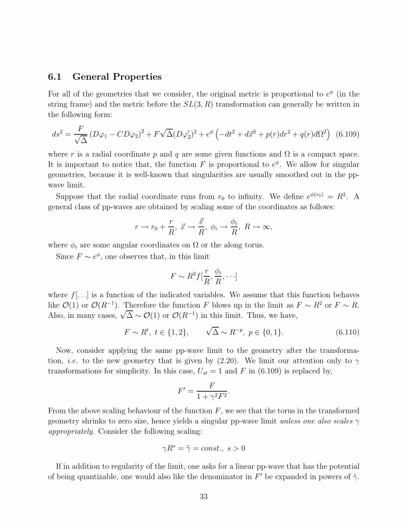
6.1 General Properties
For all of the geometries that we consider, the original metric is proportional to eφ (in the
string frame) and the metric before the SL(3, R) transformation can generally be written in
the following form:
ds2 =F√∆
(Dϕ1 − CDϕ2)2 + F
√∆(Dϕ′
2)2 + eφ
(
−dt2 + d~x2 + p(r)dr2 + q(r)dΩ2)
(6.109)
where r is a radial coordinate p and q are some given functions and Ω is a compact space.
It is important to notice that, the function F is proportional to eφ. We allow for singular
geometries, because it is well-known that singularities are usually smoothed out in the pp-
wave limit.
Suppose that the radial coordinate runs from r0 to infinity. We define eφ(r0) = R2. A
general class of pp-waves are obtained by scaling some of the coordinates as follows:
r → r0 +r
R, ~x→ ~x
R, φi →
φiR, R → ∞,
where φi are some angular coordinates on Ω or the along torus.
Since F ∼ eφ, one observes that, in this limit
F ∼ R2f [r
R,φiR, · · ·]
where f [. . .] is a function of the indicated variables. We assume that this function behaves
like O(1) or O(R−1). Therefore the function F blows up in the limit as F ∼ R2 or F ∼ R.
Also, in many cases,√
∆ ∼ O(1) or O(R−1) in this limit. Thus, we have,
F ∼ Rt, t ∈ 1, 2,√
∆ ∼ R−p, p ∈ 0, 1. (6.110)
Now, consider applying the same pp-wave limit to the geometry after the transforma-
tion, i.e. to the new geometry that is given by (2.20). We limit our attention only to γ
transformations for simplicity. In this case, Ust = 1 and F in (6.109) is replaced by,
F ′ =F
1 + γ2F 2.
From the above scaling behaviour of the function F , we see that the torus in the transformed
geometry shrinks to zero size, hence yields a singular pp-wave limit unless one also scales γ
appropriately. Consider the following scaling:
γRs = γ = const., s > 0
If in addition to regularity of the limit, one asks for a linear pp-wave that has the potential
of being quantizable, one would also like the denominator in F ′ be expanded in powers of γ.
33
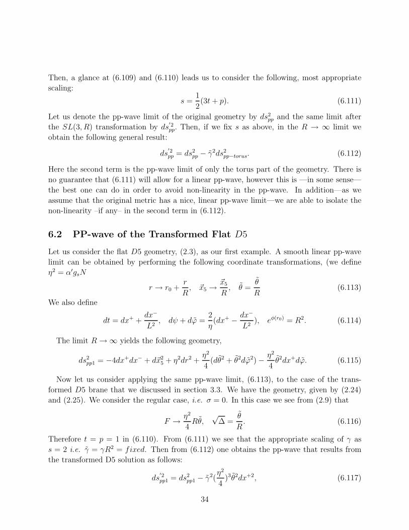
Then, a glance at (6.109) and (6.110) leads us to consider the following, most appropriate
scaling:
s =1
2(3t+ p). (6.111)
Let us denote the pp-wave limit of the original geometry by ds2pp and the same limit after
the SL(3, R) transformation by ds′2pp. Then, if we fix s as above, in the R → ∞ limit we
obtain the following general result:
ds′2pp = ds2
pp − γ2ds2pp−torus. (6.112)
Here the second term is the pp-wave limit of only the torus part of the geometry. There is
no guarantee that (6.111) will allow for a linear pp-wave, however this is —in some sense—
the best one can do in order to avoid non-linearity in the pp-wave. In addition—as we
assume that the original metric has a nice, linear pp-wave limit—we are able to isolate the
non-linearity –if any– in the second term in (6.112).
6.2 PP-wave of the Transformed Flat D5
Let us consider the flat D5 geometry, (2.3), as our first example. A smooth linear pp-wave
limit can be obtained by performing the following coordinate transformations, (we define
η2 = α′gsN
r → r0 +r
R, ~x5 →
~x5
R, θ =
θ
R(6.113)
We also define
dt = dx+ +dx−
L2, dψ + dϕ =
2
η(dx+ − dx−
L2), eφ(r0) = R2. (6.114)
The limit R → ∞ yields the following geometry,
ds2pp1 = −4dx+dx− + d~x2
5 + η2dr2 +η2
4(dθ2 + θ2dϕ2) − η2
4θ2dx+dϕ. (6.115)
Now let us consider applying the same pp-wave limit, (6.113), to the case of the trans-
formed D5 brane that we discussed in section 3.3. We have the geometry, given by (2.24)
and (2.25). We consider the regular case, i.e. σ = 0. In this case we see from (2.9) that
F → η2
4Rθ,
√∆ =
θ
R. (6.116)
Therefore t = p = 1 in (6.110). From (6.111) we see that the appropriate scaling of γ as
s = 2 i.e. γ = γR2 = fixed. Then from (6.112) one obtains the pp-wave that results from
the transformed D5 solution as follows:
ds′2pp1 = ds2
pp1 − γ2(η2
4)3θ2dx+2, (6.117)
34
where ds2pp1 is given in (6.115). We see that the SL(3, R) transformation produced a simple
γ- correction in the original pp-wave geometry. This fact was observed in [14] in case of the
deformed AdS5×S5. The string theory is quadratic and easily quantizable and one observes
that the bosonic θ field receives a correction to its mass that is proportional to γ2.
6.3 PP-wave of the Transformed D5 on S2
Let us now apply our general discussion to a slightly more complicated example: The singular
geometry of D5 brane wrapping an S2. The metric is,
ds2 = eφ[
dx21,3 +η2
(
dr2 +r(dθ2+sin2 θdϕ2)+1
4(dθ2 +sin2 θdϕ2 +(dψ+cos θdϕ+cos θdϕ)2)
)]
(6.118)
This geometry is supplied with a dilaton e2φ = e2φ0+2r√r
and an RR three form. We take a
similar geodesic as the one above (6.113):
r → r0 +r
R, θ → θ
R, θ → θ
R, ~x3 →
~x3
R, dt = dx+ +
dx−
R2, dψ+ dϕ+ dϕ =
2
η(dx+ − dx−
R2)
(6.119)
where R is again defined by eφ(r0) = R2. The following linear pp-wave geometry follows from
the R → ∞ limit:
ds2pp2 = −4dx+dx− + d~x2
3 + η2dr2 + η2r0(dθ2 + θ2dϕ2) +
η2
4(dθ2 + θ2dϕ2)− (θ2dϕ+ θ2dϕ)dx+
(6.120)
Now we consider the γ transformation where we take the same torus as is section 5.2. F
and√
∆ behaves exactly the same as in (6.116). Therefore, we also fix s = 2 and we get the
following new pp-wave from (6.112) by focusing on the same geodesic as in (6.119):
ds′2pp2 = ds2
pp2 − γ2(η2
4)3θ2dx+2 (6.121)
where ds2pp2 is given in (6.120).
6.4 PP-wave Limit of the Transformed Non-singular Solution
We finally consider the physically most interesting case of the transformed non-singular
solution. It has proved somewhat tricky to obtain a regular pp-wave limit of this solution
even before the SL(3, R) transformation. This limit is discussed in [20]. Here we first review
the argument of [20] and we revise it slightly so that it can be applied also for the case of γ
deformed non-singular background.
In order to explore the gauge dynamics at IR one is interested in a geodesic near r = 0.
With this purpose in mind, the authors of [20] considered the non-singular N = 1 geometry
35
in (3.37) and picked up a null geodesic that is on the S3 at the origin. It is tricky to find the
suitable coordinates for this geodesic essentially because of the following fact: the one-forms
wi of (2.4) that involve the angular coordinates of S3 are fibered by the S2 coordinates and
this fibration is given by the connection one form Ai. As one scales r → r/R and the angles
on S3 by φi → φ/R together, one does not obtain a metric that is suitable for the pp-wave
limit. This is because the the one-forms are O(1) near r ∼ 0 (the function a(r) approaches
to 1 as r → 0). Therefore this part of the metric blows up as R → ∞.
This only indicates that one should use a better set of coordinates that is more suitable for
the pp-wave limit of this geometry. [20] solved this problem as follows. The geometry when
Scherk-Schwarz reduced on the S3 produces an SU(2) gauged supergravity in 7D [10]. On
the other hand it is well-known that the gauge field A—that was the cause of the problem
that we mentioned above— is pure gauge at the origin, up to O(r2) corrections:
A = −idhh−1 + O(r2), h = e−iσ1 θ
2 e−iσ3 ϕ
2 . (6.122)
Here, we defined A = Ai σi
2. Therefore [20] simply gauged the O(1) part of A away by the
following gauge transformation,
A→ h1Ah+ ih−1dh, (6.123)
and then took the appropriate pp-wave limit as
r → r
R, θ → θ
R, ~x3 =
~x3
R, dt = dx+ +
dx−
R2, dψ + dϕ =
2
η(dx+ − dx−
R2). (6.124)
This limit produces the linear, quantizable pp-wave that is given in [20]. Here, we would
like to consider the same pp-wave limit that is given in (6.124) in the case of the γ deformed
solution (5.86). As the S3 of the undeformed solution is distorted by the γ transformation,
one cannot simply make a “gauge transformation” in A. Below, we explain the appropriate
way to put the metric in a suitable form.
The gauge transformation (6.123) is nothing else but a coordinate transformation on the
angular variables θ, ϕ, ψ from the 10D point of view. Explicitly, it is equivalent to changing
the coordinates as,
w → hw h−1 − idh h−1, (6.125)
where we defined w = wi σi
2. Noting that the one-forms, (2.4) on the SU(2) group manifold
are given as follows,
w = −idg g−1, g = eiσ3 ψ
2 eiσ1 θ
2 eiσ3 ϕ
2
one sees that the transformation in (6.125) is equivalent to
g → h g. (6.126)
36
where h is given in (6.122). We give the explicit form of this coordinate transformation
in Appendix E. Now we apply this coordinate transformation to the γ deformed metric in
(5.86). Using the explicit expressions in Appendix E one can work out the full coordinate
transformation of (5.86). However, it is sufficient for us to observe the following. At the end
of section 6.1 we argued that, if one knows the pp-wave limit in the undeformed solution one
can obtain the new pp-wave of the deformed solution from (6.112). Having performed the
coordinate transformation (6.126), we put the first term in (6.112) in the appropriate form
to perform the pp-wave limit in (6.124). Therefore the limit of this part will be explicitly
given as the pp-wave in [20], that is
ds2 = −2dx+dx− − 1
gsNα′(1
9~u2 + ~v2)(dx+)2 + d ~x3
2 + dz2 + d~u2 + d~v2 (6.127)
Here u and v are two-planes and z is a line. There is also an expression for the three form.
The second part in (6.112), then produces some non-linear corrections to this pp-wave that
is proportional to γ. In order to obtain a meaningful limit we found that the scaling should
be defined as follows:
γR4 = γ = const.
We explicitly see that the γ deformation produces a non-linear correction to the pp-wave
of the original solution and this deformation should be dual to the complicated dynamics
that affects the KK-sector of the N = 1 theory.
7 Deformations of the N = 2 Theory
With the fields (Aaµ, φa, ψa) mentioned in section 2, one can perform a different twisting
from the one explained there. One can choose the second U(1) to twist, inside the diagonal
combination of the SU(2)′s. That is U(1)D inside diag(SU(2)L×SU(2)R). If this is done, we
can see that the massless spectrum can be put in correspondence with a vector multiplet of
N = 2 in d=(3+1). The corresponding solution, preserves eight supercharges as was found
in [11]
ds2 = eφ(
dx21,3 +
z
λ
(
dθ2 + sin2 θdϕ2)
)
+e−φ
λ
(
dρ2 + ρ2dϕ22
)
(7.128)
+e−φ
λz
(
dσ2 + σ2(
dϕ1 + cos θdϕ)2)
, (7.129)
where λ = (gsNα′)−1. The dilaton is,
e2φ = e2z(
1 − sin2 θ1 + ce−2z
2z
)
. (7.130)
37
Here z and θ are given in terms of the radial functions that appear in (7.128) as
ρ = sin θez, σ =√z cos θez−x (7.131)
and x is the following radial function:
e−2x = 1 − 1 + ce−2z
2z. (7.132)
c is an integration constant. The RR two-form field reads,
C(2) = gsNα′ϕ2d
(
ξ(dϕ1 + cos θdϕ))
, (7.133)
where
ξ = (1 + e2x cot2 θ)−1. (7.134)
It is well-known that the R-symmetry of the theory is dual to the isometry along the ϕ2
direction. This chiral symmetry is anomalous because of the ϕ2 dependence of C(2).
7.1 Transformation along a non-R-symmetry Direction
We shall first discuss the simpler case of SL(2, R) transformations along the torus that is
composed of ϕ1 and ϕ. The metric is already in the desired form given in eq. (4.55)
ds2 = F
(
1√∆
(dϕ1 − Cdϕ+ A(1) − CA(2))2 +√
∆(dϕ+ A(2))2
)
+ gµνdxµdxν (7.135)
with,
F =σ sin θ
λ, ∆ =
e2φz2 sin2 θ
σ2, C = − cos θ, A(1) = A(2) = 0 (7.136)
and
gµνdxµdxν = eφ(dx2
1.3 +z
λdθ2) +
e−φ
λzdσ2 +
e−φ
λ(dρ2 + ρ2dϕ2
2). (7.137)
The RR two from is put in the following form:
C2 = C12(dϕ1 + A(1)) ∧ (dϕ+ A(2)) + C(1)µ (dϕ1 + A(1)) ∧ dxµ + C(2)
µ (dϕ+ A(2)) ∧ dxµ
−1
2(A(a)
µ C(a)ν − cµν)dx
µ ∧ dxν . (7.138)
Comparison of (7.133) with (7.138) yields the following components of the RR two-form:
C12 = 0, C(1)ρ = −ϕ2
λ
∂ξ
∂ρ, C
(1)σ = −ϕ2
λ
∂ξ
∂σ,
C(2)ρ = −ϕ2
λ
∂ξ
∂ρcos θ, C
(2)σ = −ϕ2
λ
∂ξ
∂σcos θ, C
(2)
θ=ϕ2
λξ sin θ, cµν = 0. (7.139)
38
The transformation yields the following results.
A′(1) = −σC(2), A′(2) = σC(1), C ′(1) = C(1), C ′(2) = C(2), c′µν = 0. (7.140)
New metric functions are given by the general formula, eq. (2.18) with C12 = 0. In the
simpler case of σ = 0 transformation one obtains,
C ′12 = 0, F ′ =
F
1 + γ2F 2, B′
12 =γF 2
1 + γ2F 2, e2φ
′
=e2φ
1 + γ2F 2, χ′ = 0. (7.141)
Now, let us see whether or not the gravity dual computations of the β-function and the
chiral anomaly are affected by the SL(2, R) transformation. We shall consider the general
transformation that depends on both σ and γ in what follows. Gravity duals of the theta
angle and the YM coupling constant can be obtained by placing a probe D5-brane on the
supersymmetric cycle σ = 0 in the geometry [28]. From the DBI action on the probe
brane one can read off the information after reducing on the S2. Essentially, the coupling
constant is determined by the volume of S2 that the D5 branes wrap and the theta angle is
determined by the flux of the RR form on this sphere. One gets the following results (before
the transformation):
1
g2=
1
2(2π)3gsα′
∫ 2π
0dϕ
∫ π
0dθe−φV ol(S2) =
N
4π2log ρ. (7.142)
θYM =1
2πgsα′
∫ 2π
0dϕ∫ π
0dθC
(2)
θϕ= −2Nϕ2. (7.143)
We consider the transformed solution determined by the transformation rules in (2.18)
and (7.140). One obtains the following result for the coupling constant:
1
g′2=
1
2(2π)3gsα′
∫ 2π
0dϕ
∫ π
0dθe−φ
′
V ol(S2)′ =1
2(2π)3gsα′
∫ 2π
0dϕ∫ π
0dθH− 1
2e−φV ol(S2).
(7.144)
Here V ol(S2)′ denotes the volume of S2 in the transformed geometry and the function H is
given by,
H = 1 + σ2 σ2
λsin2 θe−2φ. (7.145)
However one should remember to place the probe brane on the supersymmetric cycle. From
the general transformation rules under SL(2, R) it is not hard to see that σ = 0 maps to σ = 0
hence we have the same supersymmetric cycle. On this cycle one learns from (7.145) that
H = 1. Therefore we refer that the coupling function is unaffected by the transformation.
For the theta angle, one has the following new expression:
θ′YM =1
2πgsα′
∫ 2π
0dϕ∫ π
0dθC(2)′
θϕ =1
2πgsα′
∫ 2π
0dϕ∫ π
0dθ(1 − JGσ)C
(2)
θϕ. (7.146)
39
From (2.19) we see that J = 0 at the supersymmetric cycle σ = 0 (Remember that when
C12 = 0). Therefore we learn that θYM is also unaffected by the transformation. This result
is indeed expected because the particular SL(3, R) transformation that we make here is not
breaking the supersymmetry. Then, this result can be viewed as a consistency check for the
whole setup.
7.2 Transformation along the R-symmetry Directions
Now, let us work out a more complicated case of the transformation involving the torus
on the ϕ2 and ϕ angles. As ϕ2 was identified with the R-symmery we expect that this
transformation breaks supersymmetry. We rewrite the metric again in the form (4.55) that
makes the torus explicit.
ds2 = F
(
1√∆
(dϕ2 − Cd ˜ϕ+ A(1) − CA(2))2 +√
∆(dϕ+ A(2))2
)
+e2/3φ
F 1/3gµνdx
µdxν (7.147)
with,
gµνdxµdxν = e−2φ/3F 1/3
(
eφ(dx21.3 +
z
λdθ2) +
e−φ
λzdσ2 +
e−φ
λdρ2 +Ddϕ2
1
)
. (7.148)
Various functions that appear in the metric is determined as,
F√∆
= e−φσ2
λ, F
√∆ = eφ sin2 θ
z
λ+ e−φ cos2 θ
σ2
zλ,
D = e−φσ2
zλ− F
√∆A(2)
ϕ1
2, A(2) = e−ϕ
σ2
zλ
cos θ
F√
∆dϕ1, (7.149)
A(1) = C = 0. (7.150)
The RR two-form is written,
C2 = C12(dϕ2 + A(1)) ∧ (dϕ+ A(2)) + C(1)µ (dϕ2 + A(1)) ∧ dxµ + C(2)
µ (dϕ+ A(2)) ∧ dxµ
−1
2(A(a)
µ C(a)ν − cµν)dx
µ ∧ dxν . (7.151)
Comparison of (7.133) with (7.151) yields the following components of the RR two-form:
C12 = 0, C(1)µ = 0, C(2)
ρ = −ϕ2
λ
∂ξ
∂ρcos θ,
C(2)σ = −ϕ2
λ
∂ξ
∂σcos θ, C
(2)
θ=ϕ2
λξ sin θ, cµν = 0, cϕ1σ =
ϕ2
λ
∂ξ
∂σ(1
2cos θ − 1),
cϕ1ρ =ϕ2
λ
∂ξ
∂ρ(1
2cos θ − 1), cϕ1θ
= −ϕ2
λξ sin θ.
40
The transformation yields the following results.
A′(1) = −σC(2), A′(2) = A(2), C ′(1) = 0, C ′(2) = C(2), c′µν = cµν . (7.152)
New metric functions are given by the general formula, eq. (2.18) with C12 = 0.
For the new coupling constant and the new theta angle it is not hard to see that one
would get exactly the same results had one allowed to put the probe brane at the would-be
susy cycle σ = 0. However as the transformation breaks supersymmetry, σ = 0 is not a
supersymmetric cycle anymore. Therefore one does not trust the computations of the beta
function and the theta angle in this deformed solution. It will be interesting to study these
issues further.
8 Summary and Conclusions
In this paper we studied in detail the proposal of Lunin and Maldacena[14], that is to
interpret particular SL(3, R) transformations of supergravity backgrounds as duals to field
theories where the product between fields have been modified in a particular way.
We considered the quantum theories that correspond to the β deformations of D5 branes
and analyzed the regularity of the transformed configuration.
More importantly, we applied this to models that are argued to be dual to the strong
coupling regime of N = 1, 2 SYM. In this case, β transformations affect the so called KK
modes of the theory, that can be thought as ‘contaminating’ the pure SYM theory in the
supergravity approximation. We argued by a simple dipole field theory computation that
the γ deformations increase the mass of the KK modes. However they do not directly
affect the pure gauge dynamics. We confirmed these expectations from the supergravity side
by computing some field theory observables in the transformed supergravity backgrounds.
When these quantities were purely of field theory origin, no modifications were observed,
thus providing a check for the original proposal. We also showed that, as a consequence of
the transformations, there is an increase in the mass of the KK modes, hence the decoupling
is improved. We would also like to stress here the fact that in these transformed geometries,
the dilaton does not blow at infinity. This fact was already observed in the non-commutative
case and here we extend it for all β deformations.
We have studied pp-waves of the configurations that are mentioned above. In this case,
these pp waves are dual to some condensates of KK modes called annulons. We have studied
changes in the dynamics of these annulons.
As a check of consistency, we also computed the dual to N = 1 non-commutative SYM
with the methods explained here and obtained the solution previously studied by [33]. This
is in Appendix B.
Let us now comment on possible further work. It should be interesting to study the
41
physical effects of these transformations on observables of the field theory. For example,
by considering Wilson loops that wrap the transformed directions one could get some infor-
mation that depends on the deformation parameters. Also, the study of strings rotating in
the internal space could yield additional information. Another field theory quantity that is
interesting to study, and that is not expected to change, is the law obeyed by the tensions
of confining strings. These models usually obey a sine law behaviour [32].
We did not check explicitly the SUSY of the deformed backgrounds, but we expect that,
unless where we indicated, the same spinors will be preserved. In this line, it should be
interesting to study the SUSY holomorphic two cycles to place probe D5 branes in the
deformed geometry. This is interesting for the quenched SQCD and meson dynamics as
studied in [22]. It is possible that some of the holomorphic two cycles found in [22] do
indeed change. These changes should be reflected in the dynamics and spectrum of mesons.
It will also be interesting to study the glueballs of the transformed models. Indeed,
since one of the problems of studying glueballs from a supergravity perspective is that we
cannot disentangle those glueballs that belong to the original field theory from those that are
coming from KK modes, the study of this spectrum for the transformed models is interesting
because in the comparison we might be able to identify what belongs to the field theory we
are interested in and what is an artifact of the supergravity approximation. In this line, one
can study the possibility of finding massless glueballs, following what is done in [36]. In this
case, the asymptotic behavior of the dilaton in the transformed solution is different, thus it
might be possible to find a massless glueball. However, this should be analyzed in detail. A
study of the transformed family of metrics developed in [37] may also be interesting.
We also note that a more detailed study of the annulons in these confining models is
required. The annulons are precisely made of the part of the spectrum that is modified by
the SL(3, R) transformations.
It should also be of interest to study the G2 holonomy manifolds in M theory. These
backgrounds can be thought of as coming from D6 branes wrapping a three manifold inside
a CY 3−fold. There are at least three U(1)’s that can be identified (see [34], for a summary
on these geometries and the explicit expression of the U(1)’s of interest). It should also be
of interest to study different geometries, like the ones found by Pando-Zayas and Tseytlin
[35]. As well as other geometries in massive IIA; for example the duals of CFT’s in five and
three dimensions that are constructed in [38] also present all the necessary characteristics
for the SL(3, R) transformations to be applied. Computing observables in these transformed
geometries could be a way of understanding better the dual field theories.
To end this paper, we want to stress that the differences and similarities between the
original confining model and the transformed one leads us, by comparison, to a better un-
derstanding of the Physics underlying these models.
42
9 Acknowledgments
We would like to thank Changhyun Ahn, Dan Freedman, Joanna Karczmarek, Ingo Kirsch,
Martin Kruczenski, Juan Martin Maldacena, Angel Paredes-Galan, Leo Pando-Zayas, Martin
Schvellinger, Alfonso Ramallo for discussion, comments and correspondence that helped
improving the presentation of this work. This work was supported in part by funds provided
by the U.S.Department of Energy (DoE) under cooperative research agreement DF-FC02-
94ER408818. Carlos Nunez is a Pappalardo Fellow.
A Appendix: Solution Generating Technique
In this appendix we summarize the technique which was used to generate supergravity solu-
tions presented in the paper [14].
Let us write the most general configuration in IIB as
ds2IIB = F
[
1√∆
(Dϕ1 − C(Dϕ2))2 +√
∆(Dϕ2)2
]
+e2φ/3
F 1/3gµνdx
µdxν ,
B = B12(Dϕ1) ∧ (Dϕ2) +
B1µ(Dϕ1) +B2µ(Dϕ
2)
∧ dxµ
−1
2Amµ Bmνdx
µ ∧ dxν +1
2bµνdx
µ ∧ dxν
e2Φ = e2φ, C(0) = χ
C(2) = C12(Dϕ1) ∧ (Dϕ2) +
C1µ(Dϕ1) + C2µ(Dϕ
2)
∧ dxµ
−1
2Amµ Cmνdx
µ ∧ dxν +1
2cµνdx
µ ∧ dxν
C(4) = −1
2(dµν +B12cµν − ǫmnBmµCnν − B12A
mµ Cmν)dx
µdxνDϕ1Dϕ2
+1
6(Cµνλ + 3(bµν + A1
µB1ν − A2µB2ν)C1λ)dx
µdxνdxλDϕ1 + (A.1)
+dµ1µ2µ3µ4dxµ1dxµ2dxµ3dxµ4 + dµ1µ2µ3
dxµ1dxµ2dxµ3Dϕ2
where as defined in the main text of this paper
Dϕ2 = dϕ2 + A2, Dϕ1 = dϕ1 + A1 (A.2)
We have three objects which transform as vectors (see also (2.13)-(2.14) in the main text):
V (1)µ =
−B2µ
A1µ
C2µ
, V (2)µ =
B1µ
A2µ
−C1µ
: V (i)µ → (ΛT )−1V (i)
µ ; (A.3)
Wµν =
cµνdµνbµν
→ ΛWµν (A.4)
43
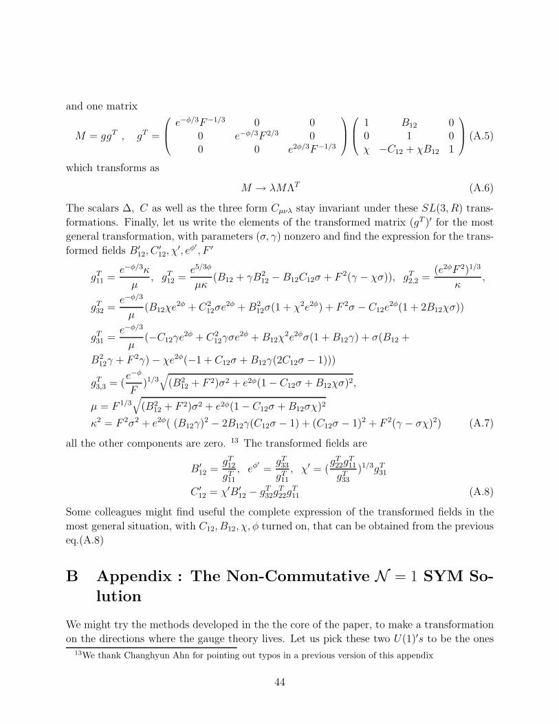
and one matrix
M = ggT , gT =
e−φ/3F−1/3 0 00 e−φ/3F 2/3 00 0 e2φ/3F−1/3
1 B12 00 1 0χ −C12 + χB12 1
(A.5)
which transforms as
M → λMΛT (A.6)
The scalars ∆, C as well as the three form Cµνλ stay invariant under these SL(3, R) trans-
formations. Finally, let us write the elements of the transformed matrix (gT )′ for the most
general transformation, with parameters (σ, γ) nonzero and find the expression for the trans-
formed fields B′12, C
′12, χ
′, eφ′
, F ′
gT11 =e−φ/3κ
µ, gT12 =
e5/3φ
µκ(B12 + γB2
12 − B12C12σ + F 2(γ − χσ)), gT2,2 =(e2φF 2)1/3
κ,
gT32 =e−φ/3
µ(B12χe
2φ + C212σe
2φ +B212σ(1 + χ2e2φ) + F 2σ − C12e
2φ(1 + 2B12χσ))
gT31 =e−φ/3
µ(−C12γe
2φ + C212γσe
2φ + B12χ2e2φσ(1 +B12γ) + σ(B12 +
B212γ + F 2γ) − χe2φ(−1 + C12σ +B12γ(2C12σ − 1)))
gT3,3 = (e−φ
F)1/3
√
(B212 + F 2)σ2 + e2φ(1 − C12σ +B12χσ)2,
µ = F 1/3√
(B212 + F 2)σ2 + e2φ(1 − C12σ +B12σχ)2
κ2 = F 2σ2 + e2φ( (B12γ)2 − 2B12γ(C12σ − 1) + (C12σ − 1)2 + F 2(γ − σχ)2) (A.7)
all the other components are zero. 13 The transformed fields are
B′12 =
gT12gT11
, eφ′
=gT33gT11
, χ′ = (gT22g
T11
gT33)1/3gT31
C ′12 = χ′B′
12 − gT32gT22g
T11 (A.8)
Some colleagues might find useful the complete expression of the transformed fields in the
most general situation, with C12, B12, χ, φ turned on, that can be obtained from the previous
eq.(A.8)
B Appendix : The Non-Commutative N = 1 SYM So-
lution
We might try the methods developed in the the core of the paper, to make a transformation
on the directions where the gauge theory lives. Let us pick these two U(1)′s to be the ones13We thank Changhyun Ahn for pointing out typos in a previous version of this appendix
44
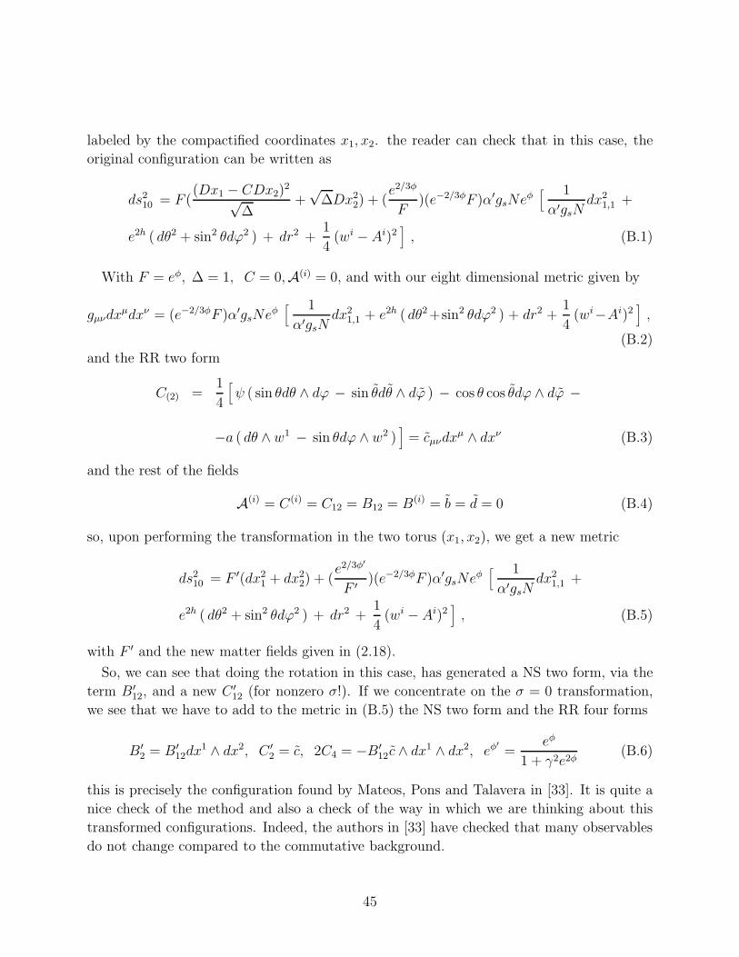
labeled by the compactified coordinates x1, x2. the reader can check that in this case, the
original configuration can be written as
ds210 = F (
(Dx1 − CDx2)2
√∆
+√
∆Dx22) + (
e2/3φ
F)(e−2/3φF )α′gsNe
φ[ 1
α′gsNdx2
1,1 +
e2h ( dθ2 + sin2 θdϕ2 ) + dr2 +1
4(wi − Ai)2
]
, (B.1)
With F = eφ, ∆ = 1, C = 0,A(i) = 0, and with our eight dimensional metric given by
gµνdxµdxν = (e−2/3φF )α′gsNe
φ[ 1
α′gsNdx2
1,1 + e2h ( dθ2+sin2 θdϕ2 ) + dr2 +1
4(wi−Ai)2
]
,
(B.2)
and the RR two form
C(2) =1
4
[
ψ ( sin θdθ ∧ dϕ − sin θdθ ∧ dϕ ) − cos θ cos θdϕ ∧ dϕ −
−a ( dθ ∧ w1 − sin θdϕ ∧ w2 )]
= cµνdxµ ∧ dxν (B.3)
and the rest of the fields
A(i) = C(i) = C12 = B12 = B(i) = b = d = 0 (B.4)
so, upon performing the transformation in the two torus (x1, x2), we get a new metric
ds210 = F ′(dx2
1 + dx22) + (
e2/3φ′
F ′)(e−2/3φF )α′gsNe
φ[ 1
α′gsNdx2
1,1 +
e2h ( dθ2 + sin2 θdϕ2 ) + dr2 +1
4(wi − Ai)2
]
, (B.5)
with F ′ and the new matter fields given in (2.18).
So, we can see that doing the rotation in this case, has generated a NS two form, via the
term B′12, and a new C ′
12 (for nonzero σ!). If we concentrate on the σ = 0 transformation,
we see that we have to add to the metric in (B.5) the NS two form and the RR four forms
B′2 = B′
12dx1 ∧ dx2, C ′
2 = c, 2C4 = −B′12c ∧ dx1 ∧ dx2, eφ
′
=eφ
1 + γ2e2φ(B.6)
this is precisely the configuration found by Mateos, Pons and Talavera in [33]. It is quite a
nice check of the method and also a check of the way in which we are thinking about this
transformed configurations. Indeed, the authors in [33] have checked that many observables
do not change compared to the commutative background.
45
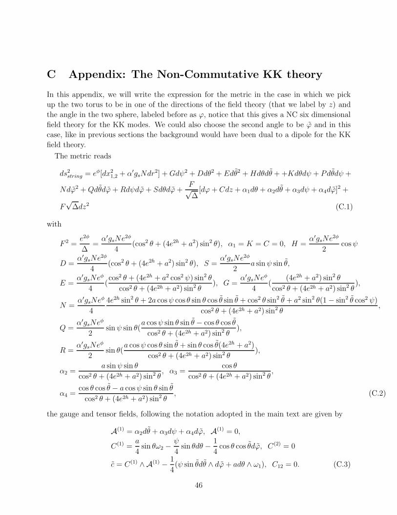
C Appendix: The Non-Commutative KK theory
In this appendix, we will write the expression for the metric in the case in which we pick
up the two torus to be in one of the directions of the field theory (that we label by z) and
the angle in the two sphere, labeled before as ϕ, notice that this gives a NC six dimensional
field theory for the KK modes. We could also choose the second angle to be ϕ and in this
case, like in previous sections the background would have been dual to a dipole for the KK
field theory.
The metric reads
ds2string = eφ[dx2
1,2 + α′gsNdr2] +Gdψ2 +Ddθ2 + Edθ2 +Hdθdθ + +Kdθdψ + Pdθdψ +
Ndϕ2 +Qdθdϕ+Rdψdϕ+ Sdθdϕ+F√∆
[dϕ+ Cdz + α1dθ + α2dθ + α3dψ + α4dϕ]2 +
F√
∆dz2 (C.1)
with
F 2 =e2φ
∆=α′gsNe
2φ
4(cos2 θ + (4e2h + a2) sin2 θ), α1 = K = C = 0, H =
α′gsNe2φ
2cosψ
D =α′gsNe
2φ
4(cos2 θ + (4e2h + a2) sin2 θ), S =
α′gsNe2φ
2a sinψ sin θ,
E =α′gsNe
φ
4(cos2 θ + (4e2h + a2 cos2 ψ) sin2 θ
cos2 θ + (4e2h + a2) sin2 θ), G =
α′gsNeφ
4(
(4e2h + a2) sin2 θ
cos2 θ + (4e2h + a2) sin2 θ),
N =α′gsNe
φ
4
4e2h sin2 θ + 2a cosψ cos θ sin θ cos θ sin θ + cos2 θ sin2 θ + a2 sin2 θ(1 − sin2 θ cos2 ψ)
cos2 θ + (4e2h + a2) sin2 θ,
Q =α′gsNe
φ
2sinψ sin θ(
a cosψ sin θ sin θ − cos θ cos θ
cos2 θ + (4e2h + a2) sin2 θ),
R =α′gsNe
φ
2sin θ(
a cosψ cos θ sin θ + sin θ cos θ(4e2h + a2)
cos2 θ + (4e2h + a2) sin2 θ),
α2 =a sinψ sin θ
cos2 θ + (4e2h + a2) sin2 θ, α3 =
cos θ
cos2 θ + (4e2h + a2) sin2 θ,
α4 =cos θ cos θ − a cosψ sin θ sin θ
cos2 θ + (4e2h + a2) sin2 θ, (C.2)
the gauge and tensor fields, following the notation adopted in the main text are given by
A(1) = α2dθ + α3dψ + α4dϕ, A(1) = 0,
C(1) =a
4sin θω2 −
ψ
4sin θdθ − 1
4cos θ cos θdϕ, C(2) = 0
c = C(1) ∧A(1) − 1
4(ψ sin θdθ ∧ dϕ+ adθ ∧ ω1), C12 = 0. (C.3)
46
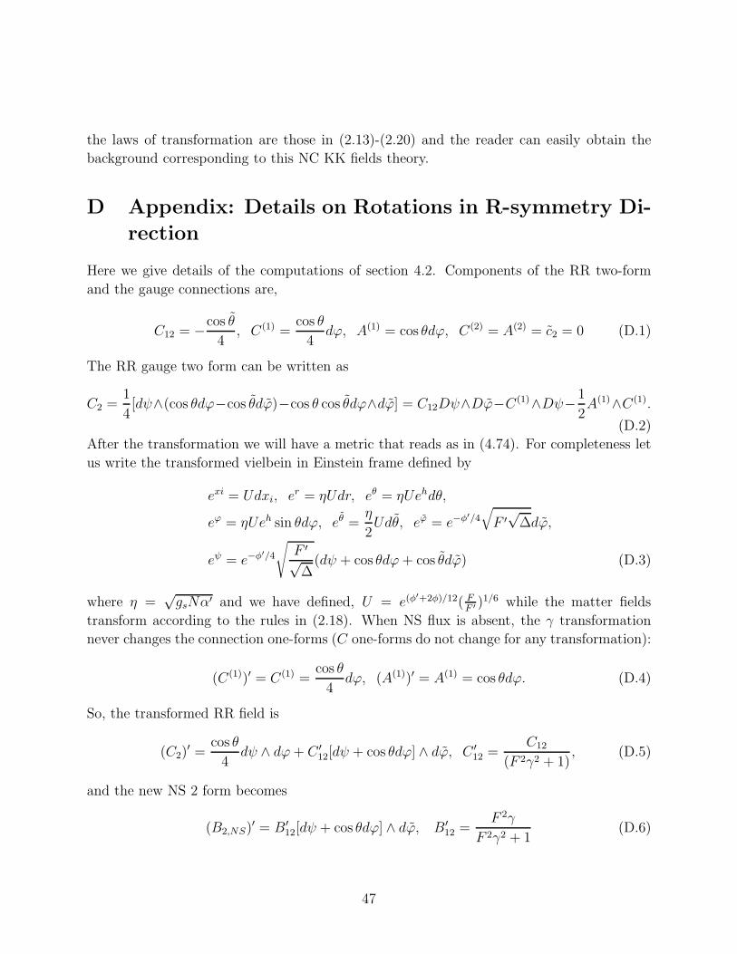
the laws of transformation are those in (2.13)-(2.20) and the reader can easily obtain the
background corresponding to this NC KK fields theory.
D Appendix: Details on Rotations in R-symmetry Di-
rection
Here we give details of the computations of section 4.2. Components of the RR two-form
and the gauge connections are,
C12 = −cos θ
4, C(1) =
cos θ
4dϕ, A(1) = cos θdϕ, C(2) = A(2) = c2 = 0 (D.1)
The RR gauge two form can be written as
C2 =1
4[dψ∧(cos θdϕ−cos θdϕ)−cos θ cos θdϕ∧dϕ] = C12Dψ∧Dϕ−C(1)∧Dψ− 1
2A(1)∧C(1).
(D.2)
After the transformation we will have a metric that reads as in (4.74). For completeness let
us write the transformed vielbein in Einstein frame defined by
exi = Udxi, er = ηUdr, eθ = ηUehdθ,
eϕ = ηUeh sin θdϕ, eθ =η
2Udθ, eϕ = e−φ
′/4
√
F ′√
∆dϕ,
eψ = e−φ′/4
√
F ′√
∆(dψ + cos θdϕ+ cos θdϕ) (D.3)
where η =√gsNα′ and we have defined, U = e(φ
′+2φ)/12( FF ′
)1/6 while the matter fields
transform according to the rules in (2.18). When NS flux is absent, the γ transformation
never changes the connection one-forms (C one-forms do not change for any transformation):
(C(1))′ = C(1) =cos θ
4dϕ, (A(1))′ = A(1) = cos θdϕ. (D.4)
So, the transformed RR field is
(C2)′ =
cos θ
4dψ ∧ dϕ+ C ′
12[dψ + cos θdϕ] ∧ dϕ, C ′12 =
C12
(F 2γ2 + 1), (D.5)
and the new NS 2 form becomes
(B2,NS)′ = B′
12[dψ + cos θdϕ] ∧ dϕ, B′12 =
F 2γ
F 2γ2 + 1(D.6)
47
The new dilaton and the axion fields are, e2φ′
= e2φ
F 2γ2+1, χ′ = γC12. Let us also present the
RR field strength,
H ′3 = dB2 =
e−2h+φ′/4
η2U2
√
F ′√
∆B′
12eϕ ∧ eθ ∧ eϕ +
eφ′/2
ηF ′U(∂rB
′12e
r + 2∂θB′12e
θ) ∧ eψ ∧ eϕ (D.7)
F ′3 = dC ′
2 − χ′H ′3 =
e−2h+φ′/4
η2U2
√
F ′√
∆(C ′
12 +cos θ
4− χ′B′
12)eϕ ∧ eθ ∧ eϕ +
e−2h+φ′/4
4η2U2√
F ′
√∆
eθ ∧ eϕ ∧ eψ
+eφ
′/2
F ′ηU([∂rC
′12 − χ∂rB
′12]e
r + 2[∂θC′12 − χ∂θB
′12]e
θ) ∧ eψ ∧ eϕ. (D.8)
E Appendix: Explicit Form of the coordinate trans-
formation in Section 6.4
Defining the new coordinates as θ, ψ, ϕ, one shows that (6.126) is given by:
cos θ = cos θ cos θ − sin τ sin θ cos(ψ + ϕ),
cot ψ = cos θ cos(ψ + ϕ), (F.1)
cos ϕ sin θ = cosϕ sin θ cos θ + sin θ cos θ cos ϕ cos(ψ + ϕ) − sin θ sin ϕ sin(ψ + ϕ).(F.2)
References
[1] J. M. Maldacena, Adv. Theor. Math. Phys. 2, 231 (1998) [Int. J. Theor. Phys. 38, 1113
(1999)] [arXiv:hep-th/9711200].
[2] S. S. Gubser, I. R. Klebanov and A. M. Polyakov, Phys. Lett. B 428, 105 (1998)
[arXiv:hep-th/9802109].
[3] E. Witten, Adv. Theor. Math. Phys. 2, 253 (1998) [arXiv:hep-th/9802150].
[4] N. Itzhaki, J. M. Maldacena, J. Sonnenschein and S. Yankielowicz, Phys. Rev. D 58,
046004 (1998) [arXiv:hep-th/9802042].
[5] L. Girardello, M. Petrini, M. Porrati and A. Zaffaroni, Nucl. Phys. B 569, 451
(2000) [arXiv:hep-th/9909047]. L. Girardello, M. Petrini, M. Porrati and A. Zaffaroni,
JHEP 9905, 026 (1999) [arXiv:hep-th/9903026]. L. Girardello, M. Petrini, M. Porrati
and A. Zaffaroni, JHEP 9812, 022 (1998) [arXiv:hep-th/9810126]. D. Z. Freedman,
S. S. Gubser, K. Pilch and N. P. Warner, Adv. Theor. Math. Phys. 3, 363 (1999)
48
[arXiv:hep-th/9904017]. D. Z. Freedman, S. S. Gubser, K. Pilch and N. P. Warner,
JHEP 0007, 038 (2000) [arXiv:hep-th/9906194].
[6] J. Polchinski and M. J. Strassler, arXiv:hep-th/0003136.
[7] I. R. Klebanov and M. J. Strassler, JHEP 0008, 052 (2000) [arXiv:hep-th/0007191].
[8] K. Skenderis, Class. Quant. Grav. 19, 5849 (2002) [arXiv:hep-th/0209067].
[9] J. M. Maldacena and C. Nunez, Phys. Rev. Lett. 86, 588 (2001) [arXiv:hep-th/0008001].
[10] A. H. Chamseddine and M. S. Volkov, Phys. Rev. Lett. 79, 3343 (1997) [arXiv:hep-
th/9707176].
[11] J. P. Gauntlett, N. Kim, D. Martelli and D. Waldram, Phys. Rev. D 64, 106008 (2001)
[arXiv:hep-th/0106117]. F. Bigazzi, A. L. Cotrone and A. Zaffaroni, Phys. Lett. B 519,
269 (2001) [arXiv:hep-th/0106160].
[12] I. R. Klebanov and A. A. Tseytlin, Nucl. Phys. B 578, 123 (2000) [arXiv:hep-
th/0002159].
[13] M. Bertolini, Int. J. Mod. Phys. A 18, 5647 (2003) [arXiv:hep-th/0303160]. F. Bigazzi,
A. L. Cotrone, M. Petrini and A. Zaffaroni, theories,” Riv. Nuovo Cim. 25N12, 1
(2002) [arXiv:hep-th/0303191]. E. Imeroni, theories,” arXiv:hep-th/0312070. A. Pare-
des, arXiv:hep-th/0407013.
[14] O. Lunin and J. Maldacena, arXiv:hep-th/0502086.
[15] N. Seiberg and E. Witten, JHEP 9909, 032 (1999) [arXiv:hep-th/9908142].
[16] R. G. Leigh and M. J. Strassler, Nucl. Phys. B 447, 95 (1995) [arXiv:hep-th/9503121].
[17] A. Bergman and O. J. Ganor, JHEP 0010, 018 (2000) [arXiv:hep-th/0008030].
A. Bergman, K. Dasgupta, O. J. Ganor, J. L. Karczmarek and G. Rajesh, Phys. Rev.
D 65, 066005 (2002) [arXiv:hep-th/0103090].
[18] S. A. Frolov, R. Roiban and A. A. Tseytlin, arXiv:hep-th/0503192.
[19] S. Frolov, arXiv:hep-th/0503201.
[20] E. G. Gimon, L. A. Pando Zayas, J. Sonnenschein and M. J. Strassler, JHEP 0305, 039
(2003) [arXiv:hep-th/0212061].
49
[21] R. Apreda, F. Bigazzi and A. L. Cotrone, JHEP 0312, 042 (2003) [arXiv:hep-
th/0307055]. G. Bertoldi, F. Bigazzi, A. L. Cotrone, C. Nunez and L. A. Pando Zayas,
Nucl. Phys. B 700, 89 (2004) [arXiv:hep-th/0401031]. F. Bigazzi, A. L. Cotrone, L. Mar-
tucci and L. A. Pando Zayas, Phys. Rev. D 71, 066002 (2005) [arXiv:hep-th/0409205].
F. Bigazzi, A. L. Cotrone and L. Martucci, Nucl. Phys. B 694, 3 (2004) [arXiv:hep-
th/0403261].
[22] C. Nunez, A. Paredes and A. V. Ramallo, JHEP 0312, 024 (2003) [arXiv:hep-
th/0311201].
[23] V. Niarchos and N. Prezas, JHEP 0306, 015 (2003) [arXiv:hep-th/0212111].
[24] E. Witten, Commun. Math. Phys. 117, 353 (1988). M. Bershadsky, C. Vafa and
V. Sadov, Nucl. Phys. B 463, 420 (1996) [arXiv:hep-th/9511222].
[25] R. P. Andrews and N. Dorey, arXiv:hep-th/0505107.
[26] U. Gursoy, S. A. Hartnoll and R. Portugues, Phys. Rev. D 69, 086003 (2004) [arXiv:hep-
th/0311088]. I. R. Klebanov, P. Ouyang and E. Witten, Phys. Rev. D 65, 105007 (2002)
[arXiv:hep-th/0202056].
[27] J. Sonnenschein, arXiv:hep-th/0003032.
[28] P. Di Vecchia, A. Lerda and P. Merlatti, Nucl. Phys. B 646, 43 (2002) [arXiv:hep-
th/0205204].
[29] M. Bertolini and P. Merlatti, Phys. Lett. B 556, 80 (2003) [arXiv:hep-th/0211142].
[30] R. Apreda, F. Bigazzi, A. L. Cotrone, M. Petrini and A. Zaffaroni, Phys. Lett. B 536
(2002) 161 [arXiv:hep-th/0112236].
[31] S. A. Hartnoll and R. Portugues, Phys. Rev. D 70, 066007 (2004) [arXiv:hep-
th/0405214].
[32] C. P. Herzog and I. R. Klebanov, Phys. Lett. B 526, 388 (2002) [arXiv:hep-th/0111078].
[33] T. Mateos, J. M. Pons and P. Talavera, Nucl. Phys. B 651, 291 (2003) [arXiv:hep-
th/0209150].
[34] S. A. Hartnoll and C. Nunez, “Rotating membranes on G(2) manifolds, logarithmic
anomalous dimensions and JHEP 0302, 049 (2003) [arXiv:hep-th/0210218].
[35] L. A. Pando Zayas and A. A. Tseytlin, “3-branes on resolved conifold,” JHEP 0011,
028 (2000) [arXiv:hep-th/0010088].
50
[36] S. S. Gubser, C. P. Herzog and I. R. Klebanov, JHEP 0409, 036 (2004) [arXiv:hep-
th/0405282]. M. Schvellinger, JHEP 0409, 057 (2004) [arXiv:hep-th/0407152].
[37] A. Butti, M. Grana, R. Minasian, M. Petrini and A. Zaffaroni, supersymmetric family
JHEP 0503, 069 (2005) [arXiv:hep-th/0412187].
[38] C. Nunez, I. Y. Park, M. Schvellinger and T. A. Tran, JHEP 0104, 025 (2001)
[arXiv:hep-th/0103080].
[39] J. Gomis and H. Ooguri, Nucl. Phys. B 635, 106 (2002) [arXiv:hep-th/0202157].
51
Related Documents


![[Wess Bagger]Supersymmetry and Supergravity](https://static.cupdf.com/doc/110x72/55cf8eb6550346703b94d652/wess-baggersupersymmetry-and-supergravity.jpg)