Dipankar Bandyopadhyay, Ph.D.dbandyop/BIOS625/lecture_02_new.pdf · Inference for Binomial Parameters Dipankar Bandyopadhyay, Ph.D. Department of Biostatistics, Virginia Commonwealth

Inference for Binomial Parameters

Dipankar Bandyopadhyay, Ph.D.

Department of Biostatistics,Virginia Commonwealth University

D. Bandyopadhyay (VCU) BIOS 625: Categorical Data & GLM 1 / 58

Inference for a probability

Phase II cancer clinical trials are usually designed to see if a new,single treatment produces favorable results (proportion of success),when compared to a known, “industry standard”).

If the new treatment produces good results, then further testing willbe done in a Phase III study, in which patients will be randomized tothe new treatment or the “industry standard”.

In particular, n independent patients on the study are given just onetreatment, and the outcome for each patient is usually

Yi =

{1 if new treatment shrinks tumor (success)0 if new treatment does not shrinks tumor (failure)

,

i = 1, . . . , n

For example, suppose n = 30 subjects are given Polen Springs water,and the tumor shrinks in 5 subjects.

The goal of the study is to estimate the probability of success, get aconfidence interval for it, or perform a test about it.


Suppose we are interested in testing

H0 : p = .5

where .5 is the probability of success on the “industry standard”

As discussed in the previous lecture, there are three ML approaches we canconsider.

Wald Test (non-null standard error)

Score Test (null standard error)

Likelihood Ratio test


Wald Test

For the hypothesesH0 : p = p0

HA : p 6= p0

The Wald statistic can be written as

zW = p̂−p0SE

= p̂−p0√p̂(1−p̂)/n


Score Test

Agresti equations 1.8 and 1.9 yield

u(p0) =y

p0− n − y

1− p0

ι(p0) =n

p0(1− p0)

zS = u(p0)

[ι(p0)]1/2

= (some algebra)

= p̂−p0√p0(1−p0)/n


Application of Wald and Score Tests


H0 : p = .5,

Suppose Y = 2 and n = 10 so p̂ = .2

Then,

ZW =(.2− .5)√.2(1− .8)/10

= −2.37171

and

ZS =(.2− .5)√.5(1− .5)/10

= −1.89737

Here, ZW > ZS and at the α = 0.05 level, the statistical conclusionwould differ.


Notes about ZW and ZS

Under the null, ZW and ZS are both approximately N(0, 1) . However, ZS ’ssampling distribution is closer to the standard normal than ZW so it isgenerally preferred.

When testing H0 : p = .5,|ZW | ≥ |ZS |

i.e., ∣∣∣∣∣ (p̂ − .5)√p̂(1− p̂)/n

∣∣∣∣∣≥∣∣∣∣∣ (p̂ − .5)√

.5(1− .5)/n

∣∣∣∣∣Why ? Note that p̂(1− p̂) ≤ .5(1− .5), i.e., p(1− p) takes on its maximumvalue at p = .5 :

p .10 .20 .30 .40 .50 .60 .70 .80 .90p(1-p) .09 .16 .21 .24 .25 .24 .21 .16 .09

Since the denominator of ZW is always less than the denominator ofZS , |ZW | ≥ |ZS |


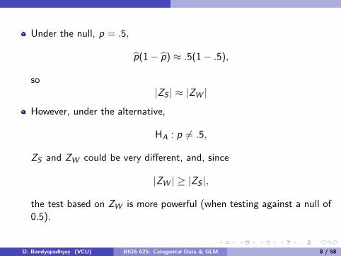
Under the null, p = .5,

p̂(1− p̂) ≈ .5(1− .5),

so|ZS | ≈ |ZW |

However, under the alternative,

HA : p 6= .5,

ZS and ZW could be very different, and, since

|ZW | ≥ |ZS |,

the test based on ZW is more powerful (when testing against a null of0.5).


For the general testH0 : p = po ,

for a specified value po , the two test statistics are

ZS =(p̂ − po)√po(1− po)/n

and

ZW =(p̂ − po)√p̂(1− p̂)/n

For this general test, there is no strict rule that

|ZW | ≥ |ZS |


Likelihood-Ratio Test

It can be shown that

2 log

{L(p̂|HA)

L(po |H0)

}= 2[log L(p̂|HA)− log L(po |H0)] ∼ χ2

1

whereL(p̂|HA) is the likelihood after replacing p by its estimate, p̂, underthe alternative (HA), and

L(po |H0)

is the likelihood after replacing p by its specified value, po , under thenull (H0).


Likelihood Ratio for Binomial Data

For the binomial, recall that the log-likelihood equals

log L(p) = log

(ny

)+ y log p + (n − y) log(1− p),


H0 : p = .5 versus H0 : p 6= .5

The likelihood ratio statistic generally only is for a two-sidedalternative (recall it is χ2 based)

Under the alternative,

log L(p̂|HA) = log

(ny

)+ y log p̂ + (n − y) log(1− p̂),

Under the null,

log L(.5|H0) = log

(ny

)+ y log .5 + (n − y) log(1− .5),


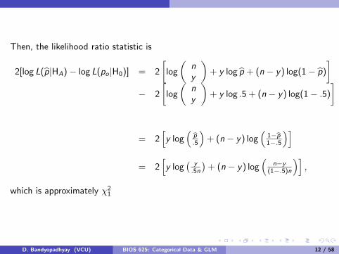
Then, the likelihood ratio statistic is

2[log L(p̂|HA)− log L(po |H0)] = 2

[log

(ny

)+ y log p̂ + (n − y) log(1− p̂)

]− 2

[log

(ny

)+ y log .5 + (n − y) log(1− .5)

]

= 2[y log

(p̂.5

)+ (n − y) log

(1−p̂1−.5

)]= 2

[y log

(y.5n

)+ (n − y) log

(n−y

(1−.5)n

)],

which is approximately χ21


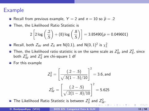
Example

Recall from previous example, Y = 2 and n = 10 so p̂ = .2

Then, the Likelihood Ratio Statistic is

2

[2 log

(.2

.5

)+ (8) log

(.8

.5

)]= 3.85490(p = 0.049601)

Recall, both ZW and ZS are N(0,1), and N(0, 1)2 is χ21

Then, the Likelihood ratio statistic is on the same scale as Z 2W and Z 2

S , sinceboth Z 2

W and Z 2S are chi-square 1 df

For this example

Z 2S =

[(.2− .5)√.5(1− .5)/10

]2= 3.6, and

Z 2W =

[(.2− .5)√.2(1− .8)/10

]2= 5.625

The Likelihood Ratio Statistic is between Z 2S and Z 2

W .


Likelihood Ratio Statistic

For the general testH0 : p = po ,

the Likelihood Ratio Statistic is

2

[y log

(p̂

po

)+ (n − y) log

(1− p̂

1− po

)]∼ χ2

1

asymptotically under the Null.


Large Sample Confidence Intervals

In large samples, since

p̂ ∼ N

(p,

p(1− p)

n

),

we can obtain a 95% confidence interval for p with

p̂ ± 1.96

√p̂(1− p̂)

n

However, since 0 ≤ p ≤ 1, we would want the endpoints of theconfidence interval to be in [0, 1], but the endpoints of this confidenceinterval are not restricted to be in [0, 1].

When p is close to 0 or 1 (so that p̂ will usually be close to 0 or 1),and/or in small samples, we could get endpoints outside of [0,1]. Thesolution would be the truncate the interval endpoint at 0 or 1.


Example

Suppose n = 10, and Y = 1, then

p̂ =1

10= .1

and the 95% confidence interval is

p̂ ± 1.96

√p̂(1− p̂)

n,

.1± 1.96

√.1(1− .1)

10,

[−.086, .2867]

After truncating, you get,[0, .2867]


Exact Test Statistics and Confidence IntervalsUnfortunately, many of the phase II trials have small samples, and theabove asymptotic test statistics and confidence intervals have very poorproperties in small samples. (A 95% confidence interval may only have80% coverage). In this situation, “Exact test statistics and ConfidenceIntervals” can be obtained.

One-sided Exact Test Statistic

The historical norm for the clinical trial you are doing is 50%, so youwant to test if the response rate of the new treatment is greater then50%.

In general, you want to test

H0:p = po = 0.5

versus

HA:p > po = 0.5


The test statistic

Y = the number of successes out of n trials

Suppose you observe yobs successes ;

Under the null hypothesis,

np̂ = Y ∼ Bin(n, po),

i.e.,

P(Y = y |H0:p = po) =

(ny

)pyo (1− po)n−y

When would you tend to reject H0:p = po in favor of HA:p > po


Answer

Under H0:p = po , you would expect p̂ ≈ po(Y ≈ npo)Under HA:p > po , you would expect p̂ > po(Y > npo)i.e., you would expect Y to be ‘large’ under the alternative.


Exact one-sided p-value

If you observe yobs successes, the exact one-sided p-value is theprobability of getting the observed yobs plus any larger (moreextreme) Y

p − value = pr(Y ≥ yobs |H0:p = po)

=∑n

j=yobs

(nj

)pjo(1− po)n−j


Other one-sided exact p-value

You want to testH0:p = po

versus

HA:p < po

The exact p-value is the probability of getting the observed yobs plusany smaller (more extreme) y

p − value = pr(Y ≤ yobs |H0:p = po)

=∑yobs

j=0

(nj

)pjo(1− po)n−j


Two-sided exact p-value

The general definition of a 2-sided exact p-value is

P

[seeing a result as likely orless likely than the observed result

∣∣∣∣∣ H0

].

It is easy to calculate a 2-sided p−value for a symmetric distribution,such as Z ∼ N(0, 1). Suppose you observe z > 0,


fontsize=fontsize=fontsize= 0.4 + ... Standard Normal Density

fontsize= | ... ...

fontsize= | . .

fontsize= | .. ..

fontsize= ******** Graph Modified to Fit on Slide *********

fontsize= | .. ..

fontsize= | . .

fontsize= | .. ..

fontsize= 0.1 + less likely .| |. less likely

fontsize= | <==== ..| |.. ====>

fontsize= | .. | | ..

fontsize= | .. | | ..

fontsize= | ... | | ...

fontsize= | .... | | ....

fontsize= 0.0 + .......... | | ..........

fontsize= | | |

fontsize= ---+--------------+--|-----------+-----------|--+--------------+--

fontsize= -4 -2 | 0 | 2 4

fontsize= | |

fontsize= -1.96 1.96

fontsize= -z z

fontsize=


Symmetric distributions

If the distribution is symmetric with mean 0, e.g., normal, then theexact 2-sided p−value is

p − value = 2 · P(Z ≥ |z |)

when z is positive or negative.

In general, if the distribution is symmetric, but not necessarilycentered at 0, then the exact 2-sided p−value is

p − value = 2 · min{P(Y ≥ yobs),P(Y ≤ yobs)}


Now, consider a symmetric binomial. For example, suppose n = 4 andpo = .5, then,

Binomial PDF for N=4 and P=0.5

Number of

Successes P(Y=y) P(Y<=y) P(Y>=y)

0 0.0625 0.0625 1.0000

1 0.2500 0.3125 0.9375

2 0.3750 0.6875 0.6875

3 0.2500 0.9375 0.3125

4 0.0625 1.0000 0.0625


Suppose you observed yobs = 4, then the exact two-sided p-value would be

p − value = 2 ·min{pr(Y ≥ yobs), pr(Y ≤ yobs)}

= 2 ·min{pr(Y ≥ 4),pr(Y ≤ 4)}

= 2 ·min{.0625, 1}

= 2(.0625)

= .125


The two-sided exact p-value is trickier when the binomial distributionis not symmetric

For the binomial data, the exact 2-sided p-value is

P

seeing a result as likely orless likely than the observedresult in either direction

∣∣∣∣∣ H0 : p = po

.Essentially the sum of all probabilities such thatP(Y = y |P0) ≤ P(yobs |P0)


In general, to calculate the 2-sided p−value1 Calculate the probability of the observed result under the null

π = P(Y = yobs |p = po) =

(n

yobs

)pyobso (1− po)n−yobs

2 Calculate the probabilities of all n + 1 values that Y can take on:

πj = P(Y = j |p = po) =

(nj

)pjo(1− po)n−j ,

j = 0, . . . , n.3 Sum the probabilities πj in (2.) that are less than or equal to the

observed probability π in (1.)

p − value =n∑

j=0

πj I (πj ≤ π) where

I (πj ≤ π) =

{1 if πj ≤ π0 if πj > π

.


Suppose n = 5, you hypothesize p = .4 and we observe y = 3successes.

Then, the PDF for this binomial is

Binomial PDF for N=5 and P=0.4

Number of

Successes P(Y=y) P(Y<=y) P(Y>=y)

0 0.07776 0.07776 1.00000

1 0.25920 0.33696 0.92224

2 0.34560 0.68256 0.66304

3 0.23040 0.91296 0.31744 <----Y obs

4 0.07680 0.98976 0.08704

5 0.01024 1.00000 0.01024


Exact p-value by hand

Step 1: Determine P(Y = 3|n = 5,P0 = .4). In this caseP(Y = 3) = .2304.

Step 2: Calculate Table (see previous slide)

Step 3: Sum probabilities less than or equal to the one observed instep 1. When Y ∈ {0, 3, 4, 5}, P(Y ) ≤ 0.2304.

ALTERNATIVE EXACT PROBS

HA: p > .4 .317 P[Y ≥ 3]HA: p < .4 .913 P[Y ≤ 3]

HA: p 6= .4 .395 P[Y ≥ 3] +P[Y = 0]


Comparison to Large Sample Inference

Note that the exact and asymptotic do not agree very well:

LARGEALTERNATIVE EXACT SAMPLEHA: p > .4 .317 .181HA: p < .4 .913 .819HA: p 6= .4 .395 .361


We will look at calculations by

1 STATA (best)

2 R (good)

3 SAS (surprisingly poor)


The following STATA code will calculate the exact p-value for you

From within STATA at the dot, type

bitesti 5 3 .4

----------Output-------------------------------------------

N Observed k Expected k Assumed p Observed p

------------------------------------------------------------

5 3 2 0.40000 0.60000

Pr(k >= 3) = 0.317440 (one-sided test)

Pr(k <= 3) = 0.912960 (one-sided test)

Pr(k <= 0 or k >= 3) = 0.395200 (two-sided test)


To perform an exact binomial test in R

Use the binom.test function available in R package stats

> binom.test(3, 5, p = 0.4, alternative = "two.sided")

Exact binomial test

data: 3 and 5

number of successes = 3, number of trials = 5, p-value = 0.3952

alternative hypothesis: true probability of success is not equal to 0.4

95 percent confidence interval:

0.1466328 0.9472550

sample estimates: probability of success

0.6

This gets a score of good since the output is not as descriptive as theSTATA output.


Interestingly, SAS Proc Freq gives the wrong 2-sided p−value

data one;

input outcome $ count;

cards;

1succ 3

2fail 2

;

proc freq data=one;

tables outcome / binomial(p=.4);

weight count;

exact binomial;

run;


---------Output-----------

Binomial Proportion

for outcome = 1succ

-----------------------------------

Test of H0: Proportion = 0.4

ASE under H0 0.2191

Z 0.9129

One-sided Pr > Z 0.1807

Two-sided Pr > |Z| 0.3613

Exact Test

One-sided Pr >= P 0.3174

Two-sided = 2 * One-sided 0.6349

Sample Size = 5


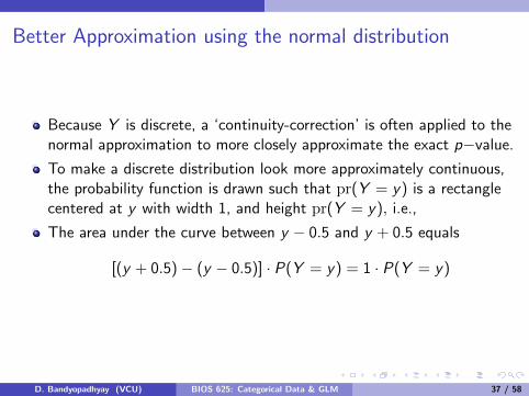
Better Approximation using the normal distribution

Because Y is discrete, a ‘continuity-correction’ is often applied to thenormal approximation to more closely approximate the exact p−value.

To make a discrete distribution look more approximately continuous,the probability function is drawn such that pr(Y = y) is a rectanglecentered at y with width 1, and height pr(Y = y), i.e.,

The area under the curve between y − 0.5 and y + 0.5 equals

[(y + 0.5)− (y − 0.5)] · P(Y = y) = 1 · P(Y = y)


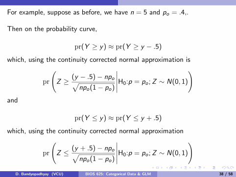
For example, suppose as before, we have n = 5 and po = .4,.

Then on the probability curve,

pr(Y ≥ y) ≈ pr(Y ≥ y − .5)

which, using the continuity corrected normal approximation is

pr

(Z ≥ (y − .5)− npo√

npo(1− po)

∣∣∣∣∣H0:p = po ;Z ∼ N(0, 1)

)and

pr(Y ≤ y) ≈ pr(Y ≤ y + .5)

which, using the continuity corrected normal approximation

pr

(Z ≤ (y + .5)− npo√

npo(1− po)

∣∣∣∣∣H0:p = po ;Z ∼ N(0, 1)

)D. Bandyopadhyay (VCU) BIOS 625: Categorical Data & GLM 38 / 58

With the continuity correction, the above p−values becomes

ContinuityCorrected

LARGE LARGEALTERNATIVE EXACT SAMPLE SAMPLE

HA: p > .4 .317 .181 .324HA: p < .4 .913 .819 .915HA: p 6= .4 .395 .361 .409

Then, even with the small sample size of n = 5, the continuity correctiondoes a good job of approximating the exact p−value.

Also, as n→∞, the exact and asymptotic are equivalent under the null;so for large n, you might as well use the asymptotic.

However, given the computational power available, you can easily calculatethe exact p-value.


Exact Confidence IntervalA (1− α) confidence interval for p is of the form

[pL, pU ],

where pL and pU are random variables such that

pr[pL ≤ p ≤ pU ] = 1− α

For example, for a large sample 95% confidence interval,

pL = p̂ − 1.96

√p̂(1− p̂)

n,

and

pU = p̂ + 1.96

√p̂(1− p̂)

n,

.D. Bandyopadhyay (VCU) BIOS 625: Categorical Data & GLM 40 / 58

It can be shown that, to obtain a 95% exact confidence interval [pL, pU ],the endpoints pL and pU satisfy

α/2 = .025 = pr(Y ≥ yobs |p = pL)

=∑n

j=yobs

(nj

)pjL(1− pL)n−j ,

andα/2 = .025 = pr(Y ≤ yobs |p = pU)

=∑yobs

j=0

(nj

)pjU(1− pU))n−j


In these formulas, we know α/2 = .025 and we know yobs and n.Then, we solve for the unknowns pL and pU .

Can figure out pL and pU by plugging different values for pL and pUuntil we find the values that make α/2 = .025

Luckily, this is implemented on the computer, so we don’t have to doit by hand.

Because of relationship between hypothesis testing and confidenceintervals, to calculate the exact confidence interval, we are actuallysetting the exact one-sided p−values to α/2 for testing Ho : p = poand solving for pL and pU .

In particular, we find pL and pU to make these p−values equal to α/2.


Example

Suppose n = 5 and yobs = 4, and we want a 95% confidence interval.(α = .05, α/2 = .025).

Then, the lower point, pL of the exact confidence interval [pL, pU ] isthe value pL such that

α/2 = .025 = pr[Y ≥ 4|p = pL] =5∑

j=4

(5j

)pjL(1− pL)n−j ,

If you don’t have a computer program to do this, you can try ‘trial’and error for pL

pL pr(Y ≥ 4|p = pL)

.240 0.013404

.275 0.022305

.2836 .025006∗ ≈ .025

Then, pL ≈ .2836.


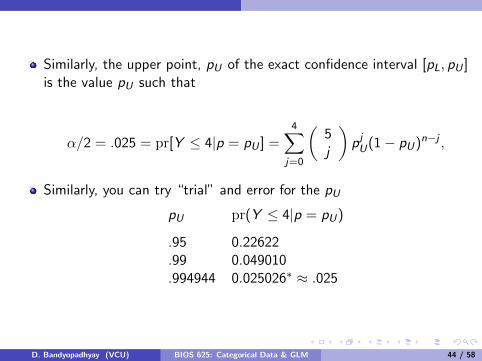
Similarly, the upper point, pU of the exact confidence interval [pL, pU ]is the value pU such that

α/2 = .025 = pr[Y ≤ 4|p = pU ] =4∑

j=0

(5j

)pjU(1− pU)n−j ,

Similarly, you can try “trial” and error for the pU

pU pr(Y ≤ 4|p = pU)

.95 0.22622

.99 0.049010

.994944 0.025026∗ ≈ .025


STATA ? The following STATA code will calculate the exact binomialconfidence interval for you

. cii 5 4

----------- Output -----------------

-- Binomial Exact --

Variable | Obs Mean Std. Err. [95% Conf. Interval]

---------+-------------------------------------------------------

| 5 .8 .1788854 .2835937 .9949219


How about SAS?

data one;

input outcome $ count;

cards;

1succ 4

2fail 1

;

proc freq data=one;

tables outcome / binomial;

weight count;

run;


Binomial Proportion

--------------------------------

Proportion 0.8000

ASE 0.1789

95% Lower Conf Limit 0.4494

95% Upper Conf Limit 1.0000

Exact Conf Limits



Test of H0: Proportion = 0.5

ASE under H0 0.2236

Z 1.3416

One-sided Pr > Z 0.0899

Two-sided Pr > |Z| 0.1797

Sample Size = 5D. Bandyopadhyay (VCU) BIOS 625: Categorical Data & GLM 47 / 58

Comparing the exact and large sample

Then, the two sided confidence intervals are

LARGESAMPLE

(NORMAL)EXACT p̂

[.2836,.9949] [.449,1]

We had to truncate the upper limit based on using p̂ at 1.

The exact CI is not symmetric about p̂ = 45 = .8, whereas the the

confidence interval based on p̂ would be if not truncated.

Suggestion; if Y < 5, and/or n < 30, use exact; for large Y and n,any of the three would be almost identical.


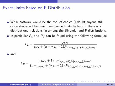
Exact limits based on F Distribution

While software would be the tool of choice (I doubt anyone stillcalculates exact binomial confidence limits by hand), there is adistributional relationship among the Binomial and F distributions.

In particular PL and PU can be found using the following formulae

PL =yobs

yobs + (n − yobs + 1)F2(n−yobs+1),2·yobs ,1−α/2

and

PU =(yobs + 1) · F2·(yobs+1),2·(n−yobs),1−α/2

(n − yobs) + (yobs + 1) · F2·(yobs+1),2·(n−yobs),1−α/2


Example using F-dist

Thus, using our example of n = 5 and yobs = 4

PL = yobsyobs+(n−yobs+1)F2(n−yobs+1),2·yobs ,1−α/2

= 44+2F4,8,0.975

= 44+2·5.0526

= 0.2836

and

PU =(yobs+1)·F2·(yobs+1),2·(n−yobs ),1−α/2

(n−yobs)+(yobs+1)·F2·(yobs+1),2·(n−yobs ),1−α/2

=5·F10,2,0.975

1+5·F10,2,0.975

= 5·39.397971+5·39.39797

= 0.9949

Therefore, our 95% exact confidence interval for p is [0.2836, 0.9949]as was observed previously


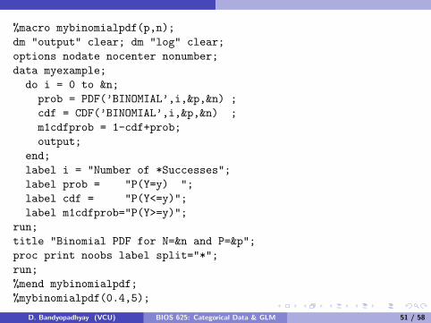
%macro mybinomialpdf(p,n);

dm "output" clear; dm "log" clear;

options nodate nocenter nonumber;

data myexample;

do i = 0 to &n;

prob = PDF(’BINOMIAL’,i,&p,&n) ;

cdf = CDF(’BINOMIAL’,i,&p,&n) ;

m1cdfprob = 1-cdf+prob;

output;

end;

label i = "Number of *Successes";

label prob = "P(Y=y) ";

label cdf = "P(Y<=y)";

label m1cdfprob="P(Y>=y)";

run;

title "Binomial PDF for N=&n and P=&p";

proc print noobs label split="*";

run;

%mend mybinomialpdf;

%mybinomialpdf(0.4,5);


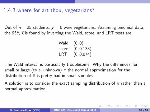
1.4.3 where for art thou, vegetarians?

Out of n = 25 students, y = 0 were vegetarians. Assuming binomial data,the 95% CIs found by inverting the Wald, score, and LRT tests are

Wald (0, 0)score (0, 0.133)LRT (0, 0.074)

The Wald interval is particularly troublesome. Why the difference? forsmall or large (true, unknown) π the normal approximation for thedistribution of π̂ is pretty bad in small samples.

A solution is to consider the exact sampling distribution of π̂ rather than anormal approximation.


1.4.4 Exact inference

An exact test proceeds as follows.

Under H0 : π = π0 we know Y ∼ bin(n, π0). Values of π̂ far away from π0,or equivalently, values of Y far away from nπ0, indicate that H0 : π = π0 isunlikely.

Say we reject H0 if Y < a or Y > b where 0 ≤ a < b ≤ n. Then we setthe type I error at α by requiring P(reject H0|H0 is true) = α. That is,

P(Y < a|π = π0) =α

2and P(Y > b|π = π0) =

α

2.


Bounding Type I error

However, since Y is discrete, the best we can do is bounding the type Ierror by choosing a as large as possible such that

P(Y < a|π = π0) =a−1∑i=0

(ni

)πi0(1− π0)n−i <

α

2,

and b as small as possible such that

P(Y > b|π = π0) =n∑

i=b+1

(ni

)πi0(1− π0)n−i <

α

2.


Exact test, cont.

For example, when n = 20, H0 : π = 0.25, and α = 0.05 we have

P(Y < 2|π = 0.25) = 0.024 and P(Y < 3|π = 0.25) = 0.091,

so a = 2. Also,

P(Y > 9|π = 0.25) = 0.014 and P(Y > 8|π = 0.25) = 0.041,

so b = 9. We reject H0 : π = 0.25 when Y < 2 or Y > 9. The type I erroris bounded: α = P(reject H0|H0 is true) ≤ 0.05, but in fact this isconservative, P(reject H0|H0 is true) = 0.024 + 0.014 = 0.038.

Nonetheless, this type of exact test can be inverted to obtain exactconfidence intervals for π. However, the actual coverage probability is atleast as large as 1− α, but typically more. So the procedure errs on theside of being conservative (CI’s are bigger than they need to be). Section16.6.1 has more details.


Tests in R

To obtain the 95% CI from inverting the score test, and from inverting theexact (Clopper-Pearson) test:

> out1=prop.test(x=0,n=25,conf.level=0.95,correct=F)

> out1$conf.int

[1] 0.0000000 0.1331923

attr(,"conf.level") [1] 0.95

> out2=binom.test(x=0,n=25,conf.level=0.95)

> out2$conf.int

[1] 0.0000000 0.1371852

attr(,"conf.level") [1] 0.95


SAS code

data table;

input vegetarian$ count @@;

datalines;

yes 0 no 25

;

* let pi be proportion of vegetarians in population;

* let’s test H0: pi=0.032 (U.S. proportion) and obtain exact 95% CI for pi;

* SAS also provides a test of H0: pi=0.5,

* other options given by binomial(ac wilson exact jeffreys)

* even though you didn’t ask for it! (not shown on next slide);

proc freq data=table order=data; weight count / zeros;

tables vegetarian / binomial testp=(0.032,0.968);

exact binomial chisq;

run;

data veg;

input response $ count;

datalines;

no 25

yes 0

;

proc freq data=veg; weight count;

tables response / binomial(ac wilson exact jeffreys) alpha

=.05; run;D. Bandyopadhyay (VCU) BIOS 625: Categorical Data & GLM 57 / 58

SAS output

The FREQ Procedure

Test Cumulative Cumulative

vegetarian Frequency Percent Percent Frequency Percent

---------------------------------------------------------------------------

yes 0 0.00 3.20 0 0.00

no 25 100.00 96.80 25 100.00

Chi-Square Test

for Specified Proportions

---------------------------------------

Chi-Square 0.8264

DF 1

Asymptotic Pr > ChiSq 0.3633

Exact Pr >= ChiSq 0.6335

WARNING: 50% of the cells have expected counts less than 5.

(Asymptotic) Chi-Square may not be a valid test.

Binomial Proportion

for vegetarian = yes

-------------------------------------

Proportion (P) 0.0000

ASE 0.0000



Exact Conf Limits



Sample Size = 25


Dipankar Bandyopadhyay, Ph.D.dbandyop/BIOS625/lecture_02_new.pdf · Inference for Binomial Parameters Dipankar Bandyopadhyay, Ph.D. Department of Biostatistics, Virginia Commonwealth

Documents