Prof. Carlos Eduardo Nigro Mazzilli Universidade de São Paulo Dinamica Non Lineare di Strutture e Sistemi Meccanici

Welcome message from author
This document is posted to help you gain knowledge. Please leave a comment to let me know what you think about it! Share it to your friends and learn new things together.
Transcript
Prof. Carlos Eduardo Nigro Mazzilli
Universidade de São Paulo
Dinamica Non Lineare di Strutture e Sistemi
Meccanici

Lezione 1
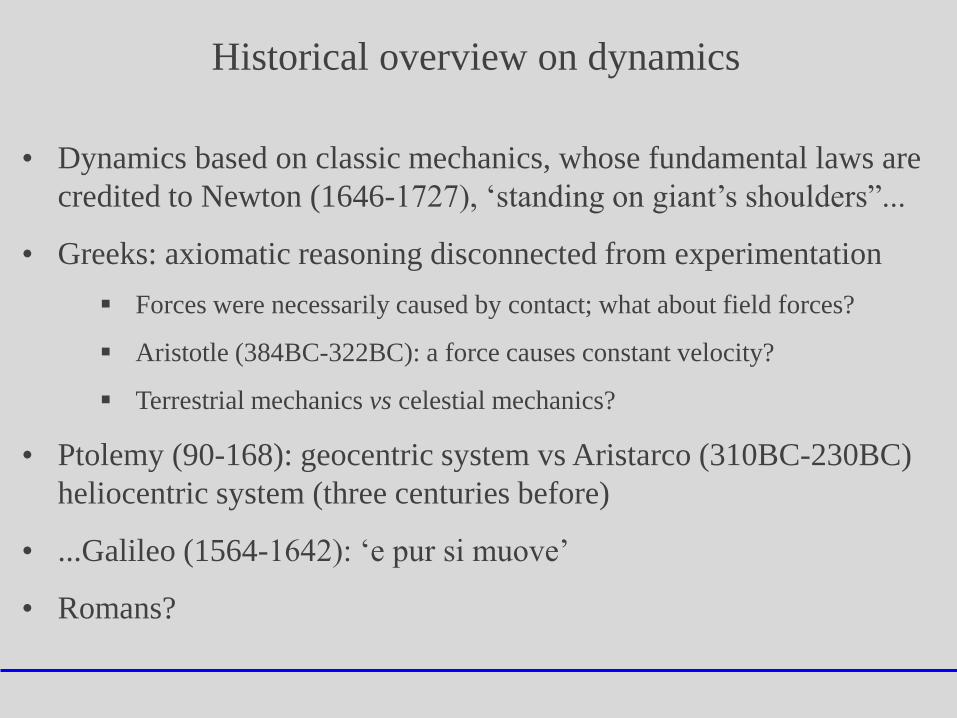
• Dynamics based on classic mechanics, whose fundamental laws are
credited to Newton (1646-1727), ‘standing on giant’s shoulders”...
• Greeks: axiomatic reasoning disconnected from experimentation
Forces were necessarily caused by contact; what about field forces?
Aristotle (384BC-322BC): a force causes constant velocity?
Terrestrial mechanics vs celestial mechanics?
• Ptolemy (90-168): geocentric system vs Aristarco (310BC-230BC)
heliocentric system (three centuries before)
• ...Galileo (1564-1642): ‘e pur si muove’
• Romans?
Historical overview on dynamics

• Moslems: from VIII to XIV centuries (Alexandria, Iberic Peninsula)
Barakat (1080-1165) denied Aristotle: force causes velocity to change...
Newton’s second law?
Alhazen (965-1040): body moves perpetually unless force obliges it to
stop or change direction... Newton’s first law?
Avempace (1095-1138): to an action corresponds a reaction... Newton’s
third law?
• Kepler, Copernicus and Galileo: celestial mechanics
• Galileo: terrestrial mechanics (displacement of a falling body
proportional to the square of time)
• Newton: law of universal gravitation and much more...
Historical overview on dynamics

Newton’s laws
First law (inertia): there are priviledged observers, called inertial observers, with
respect to whom isolated material points – that is, those subjected to null resultant
force – are at rest or in uniform rectilinear motion.
Lex I: Corpus omne perseverare in statu suo quiescendi vel movendi uniformiter in
directum, nisi quatenus a viribus impressis cogitur statum illum mutare
Historical overview on dynamics
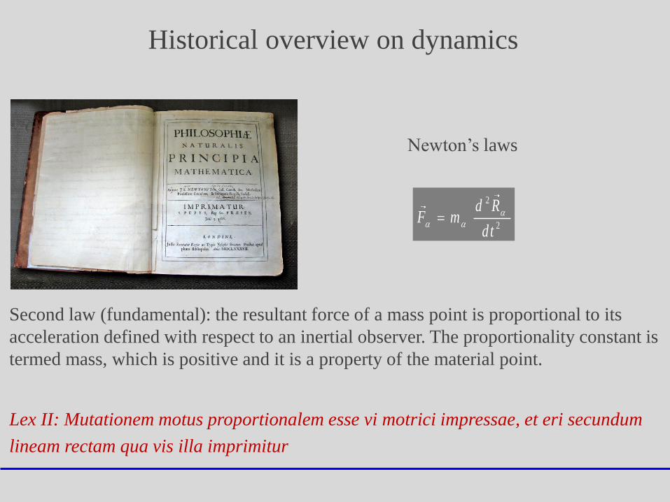
Second law (fundamental): the resultant force of a mass point is proportional to its
acceleration defined with respect to an inertial observer. The proportionality constant is
termed mass, which is positive and it is a property of the material point.
Lex II: Mutationem motus proportionalem esse vi motrici impressae, et eri secundum
lineam rectam qua vis illa imprimitur
2
2
d RF m
dt
Newton’s laws
Historical overview on dynamics
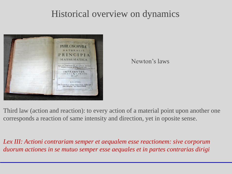
Third law (action and reaction): to every action of a material point upon another one
corresponds a reaction of same intensity and direction, yet in oposite sense.
Lex III: Actioni contrariam semper et aequalem esse reactionem: sive corporum
duorum actiones in se mutuo semper esse aequales et in partes contrarias dirigi
Newton’s laws
Historical overview on dynamics
• Newton: differential and integral calculus
• Leibniz (1646-1716): independent development of differential
calculus & fundamentals of analytical dynamics
• D’Alembert (1717-1783): principle...
• Lagrange (1736-1813): Mécanique Analytique and variational
principles
• Hamilton (1805-1865): principle...
• ...
Historical overview on dynamics
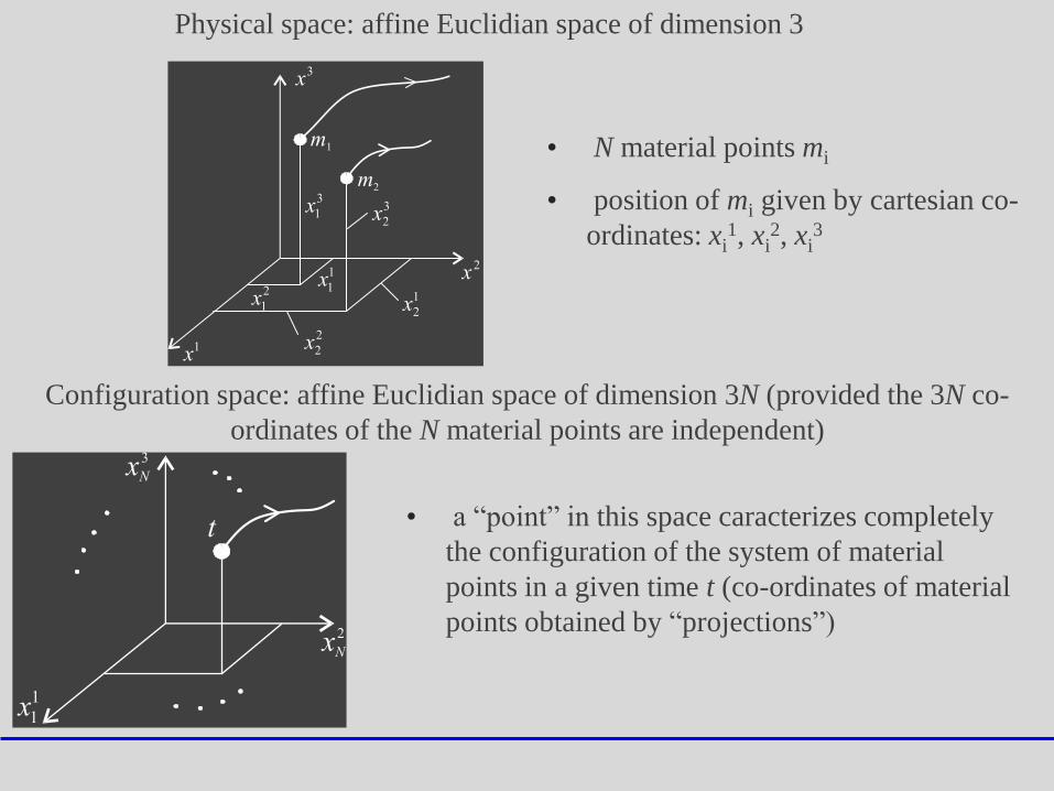
Physical space: affine Euclidian space of dimension 3
Configuration space: affine Euclidian space of dimension 3N (provided the 3N co-
ordinates of the N material points are independent)
• N material points mi
• position of mi given by cartesian co-
ordinates: xi1, xi
2, xi3
• a “point” in this space caracterizes completely
the configuration of the system of material
points in a given time t (co-ordinates of material
points obtained by “projections”)
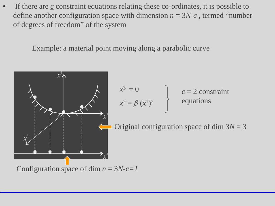
Example: a material point moving along a parabolic curve
Original configuration space of dim 3N = 3
• If there are c constraint equations relating these co-ordinates, it is possible to
define another configuration space with dimension n = 3N-c , termed “number
of degrees of freedom” of the system
x3 = 0
x2 = (x1)2
c = 2 constraint
equations
Configuration space of dim n = 3N-c=1
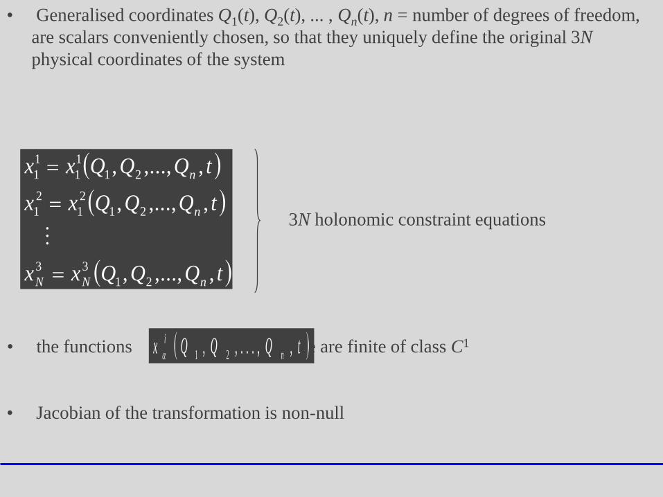
• Generalised coordinates Q1(t), Q2(t), ... , Qn(t), n = number of degrees of freedom,
are scalars conveniently chosen, so that they uniquely define the original 3N
physical coordinates of the system
tQQQxx
tQQQxx
tQQQxx
nNN
n
n
,,...,,
,,...,,
,,...,,
21
33
21
2
1
2
1
21
1
1
1
1
3N holonomic constraint equations
• the functions are are finite of class C1 tQQQx n
i ,, . . . ,, 21
• Jacobian of the transformation is non-null
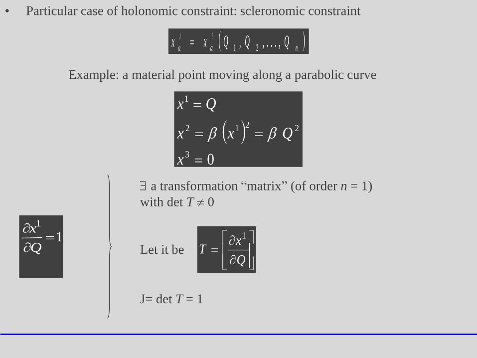
• Particular case of holonomic constraint: scleronomic constraint
03
2212
1
x
Qxx
Qx
a transformation “matrix” (of order n = 1)
with det T 0
Let it be
n
ii QQQxx , . . . ,, 21
Example: a material point moving along a parabolic curve
11
Q
x
Q
xT
1
J= det T = 1
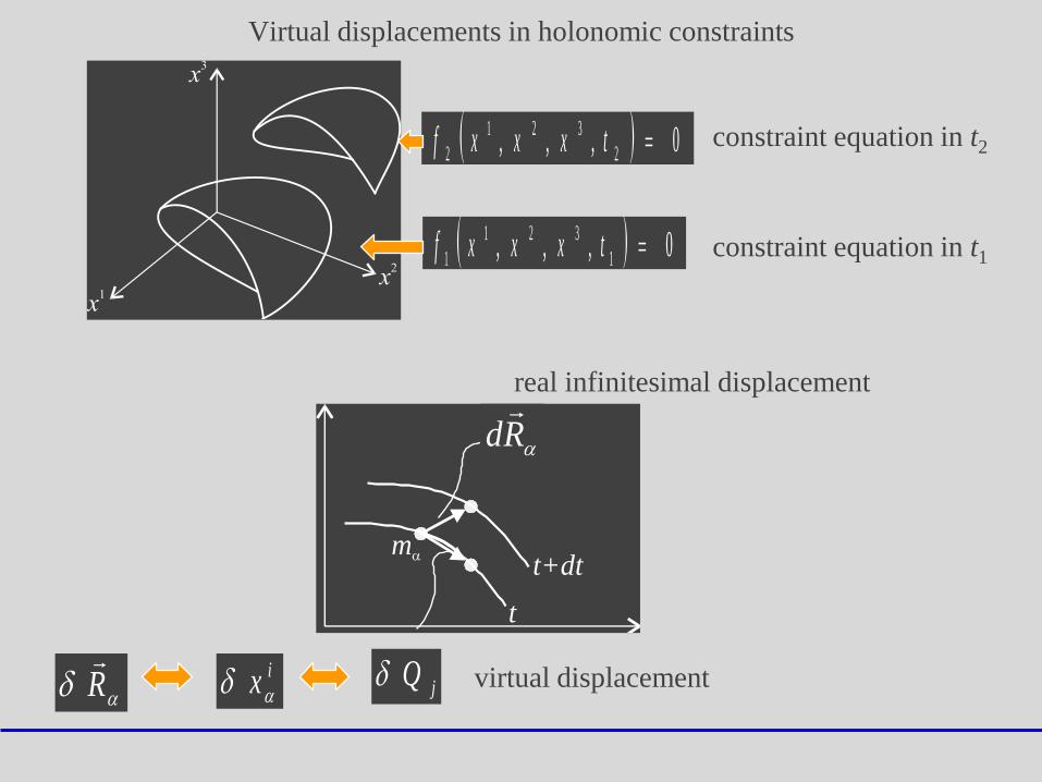
constraint equation in t2
0,,, 1
321
1 txxxf
0,,, 2
321
2 txxxf
constraint equation in t1
real infinitesimal displacement
R
virtual displacementix jQ
Virtual displacements in holonomic constraints
t
mt+dt
Rd
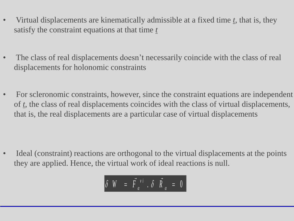
• Virtual displacements are kinematically admissible at a fixed time t, that is, they
satisfy the constraint equations at that time t
0. RFW v i
• The class of real displacements doesn’t necessarily coincide with the class of real
displacements for holonomic constraints
• For scleronomic constraints, however, since the constraint equations are independent
of t, the class of real displacements coincides with the class of virtual displacements,
that is, the real displacements are a particular case of virtual displacements
• Ideal (constraint) reactions are orthogonal to the virtual displacements at the points
they are applied. Hence, the virtual work of ideal reactions is null.
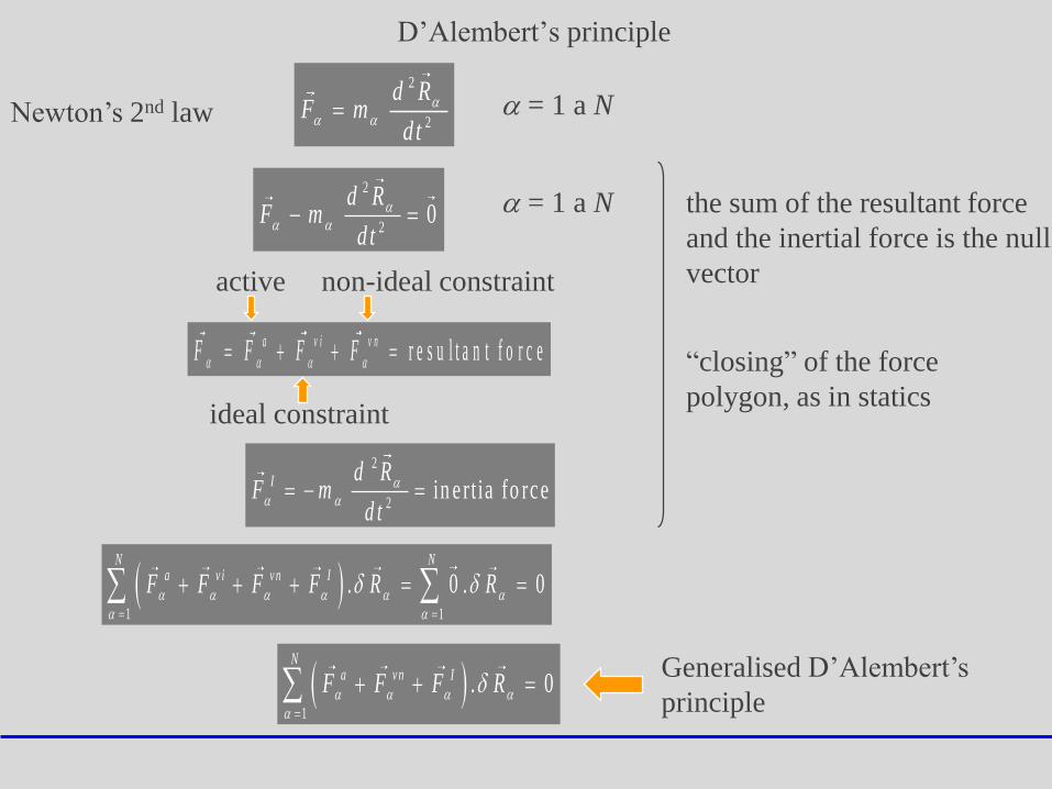
D’Alembert’s principle
the sum of the resultant force
and the inertial force is the null
vector
2
2
d RF m
dtNewton’s 2nd law = 1 a N
2
20
d R
F md t
= 1 a N
r e s u l t a n t f o r c e a v i v nF F F F
active
ideal constraint
non-ideal constraint
2
2in e rt ia fo rc e
I d RF m
d t
“closing” of the force
polygon, as in statics
1 1
. 0 . 0
N N
a v i v n IF F F F R R
1
. 0
N
a vn IF F F RGeneralised D’Alembert’s
principle
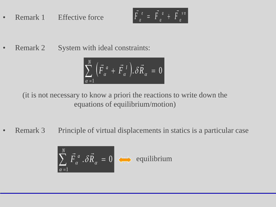
v nae FFF
• Remark 1 Effective force
(it is not necessary to know a priori the reactions to write down the
equations of equilibrium/motion)
equilibrium
• Remark 2 System with ideal constraints:
0.1
RFFN
Ia
• Remark 3 Principle of virtual displacements in statics is a particular case
0.1
RFN
a
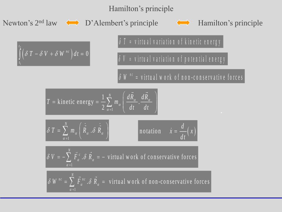
Newton’s 2nd law
Hamilton’s principle
2
1
0 t
nc
t
T V W dt
1
1kinetic energy .
2
N dR dR
T mdt d t
D’Alembert’s principle Hamilton’s principle
v i r t u a l v a r i a t i o n o f k i n e t i c e n e r g y T
1
.
N
T m R R n o ta tio n d
x xd t
1
. v i r tu a l w o rk o f c o n s e rv a t iv e fo rc e s
N
cV F R
1
. v i r tu a l w o rk o f n o n -c o n s e rv a t iv e fo rc e s
N
n c n cW F R
v i r t u a l v a r i a t i o n o f p o t e n t i a l e n e r g y V
v i r t u a l w o r k o f n o n - c o n s e r v a t i v e f o r c e s n cW
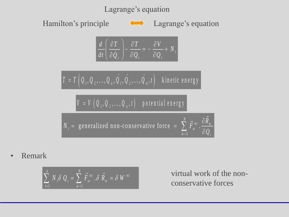
Lagrange’s equation
i
i ii
d T T VN
dt Q QQ
1 2 1 2, , . . . , , , , . . . , , k i n e t i c e n e r g yn nT T Q Q Q Q Q Q t
1 2, , . . . , , p o t e n t i a l e n e r g ynV V Q Q Q t
1
g en e ra lized n o n -co n se rv a tiv e fo rce .N
n c
i
i
RN F
Q
• Remark
1 1
.n N
n c n c
i i
i
N Q F R W
virtual work of the non-
conservative forces
Hamilton’s principle Lagrange’s equation
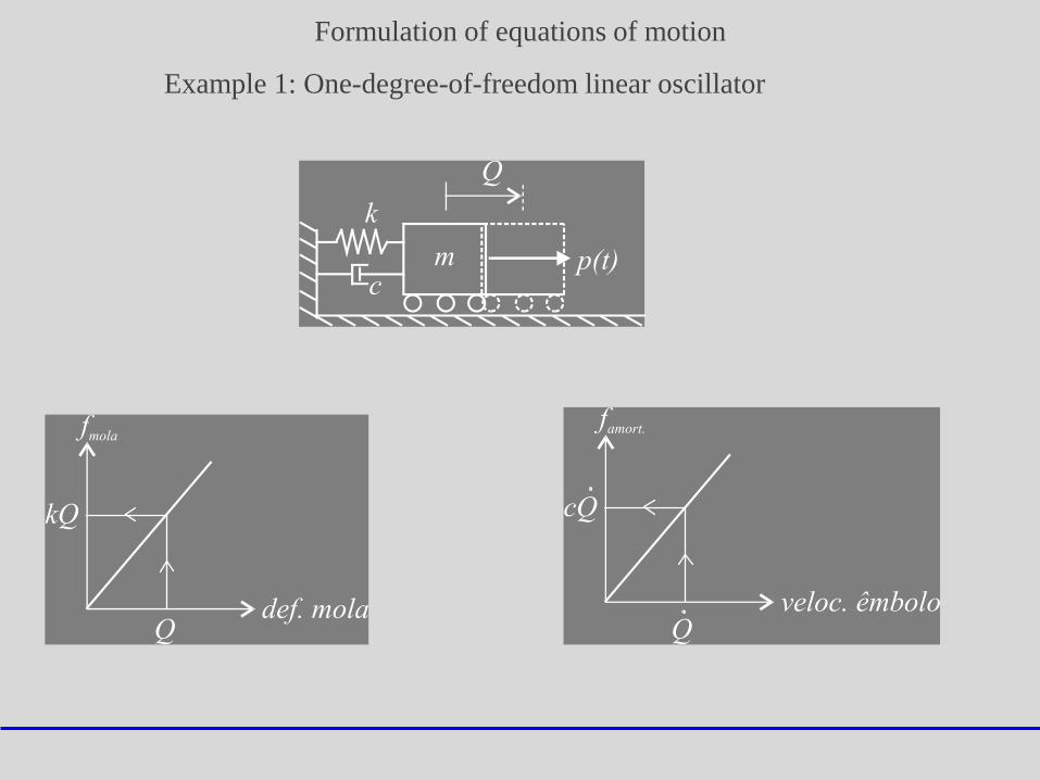
Example 1: One-degree-of-freedom linear oscillator
Formulation of equations of motion
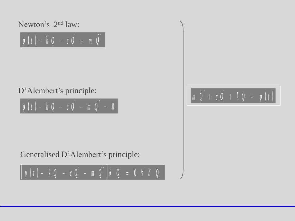
QmQck Qtp
Newton’s 2nd law:
0 QmQck Qtp
D’Alembert’s principle:
QQQmQck Qtp 0
Generalised D’Alembert’s principle:
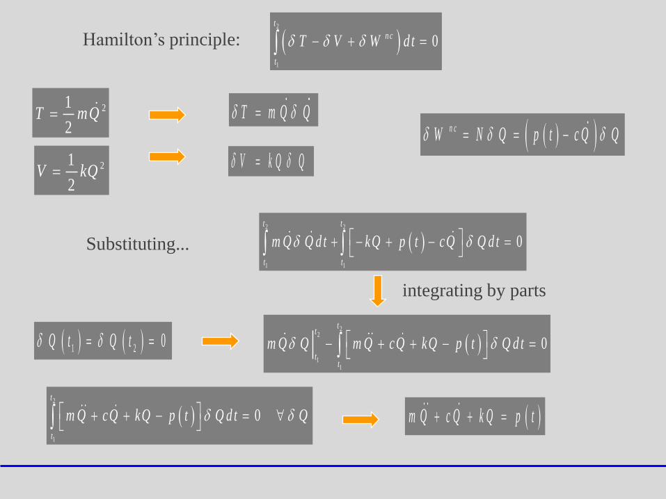
tpk QQcQm
2
1
0
t
nc
t
T V W dt Hamilton’s principle:
n cW N Q p t c Q Q
Substituting...
m Q c Q k Q p t
2 2
1 1
0
t t
t t
m Q Q d t kQ p t cQ Q d t
integrating by parts
2
2
11
0
tt
tt
m Q Q m Q cQ kQ p t Q d t 1 2 0Q t Q t
2
1
0
t
t
m Q cQ kQ p t Q d t Q
21
2T mQ
21
2V kQ
T m Q Q
V k Q Q
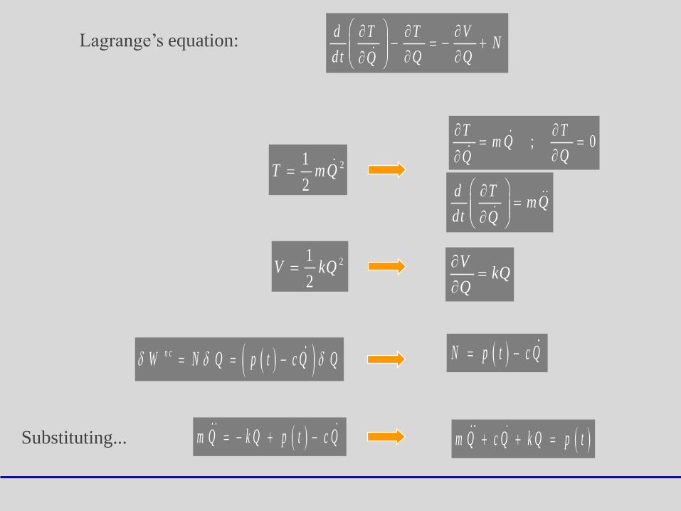
d T T VN
dt Q QQ
Lagrange’s equation:
n cW N Q p t c Q Q N p t c Q
m Q c Q k Q p t m Q k Q p t c Q Substituting...
21
2T mQ
21
2V kQ
; 0T T
m QQQ
VkQ
Q
d Tm Q
dt Q
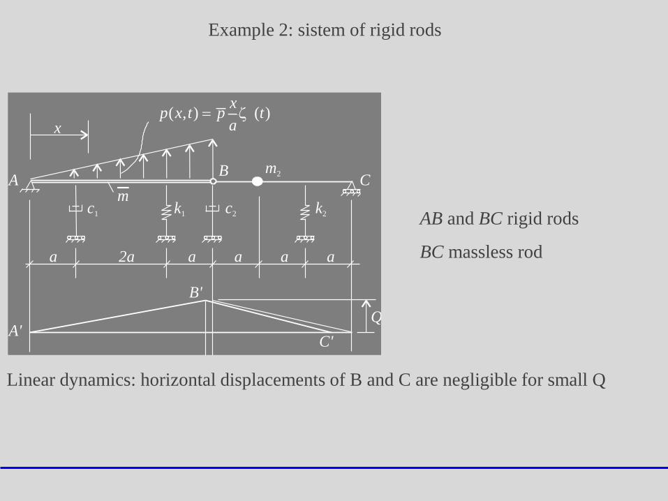
Example 2: sistem of rigid rods
AB and BC rigid rods
BC massless rod
Linear dynamics: horizontal displacements of B and C are negligible for small Q
AB
C
x
m
m2
c1 c2 k2k1
a a a a a2a
A'
B'
C'
Q
)(),( ta
xptxp
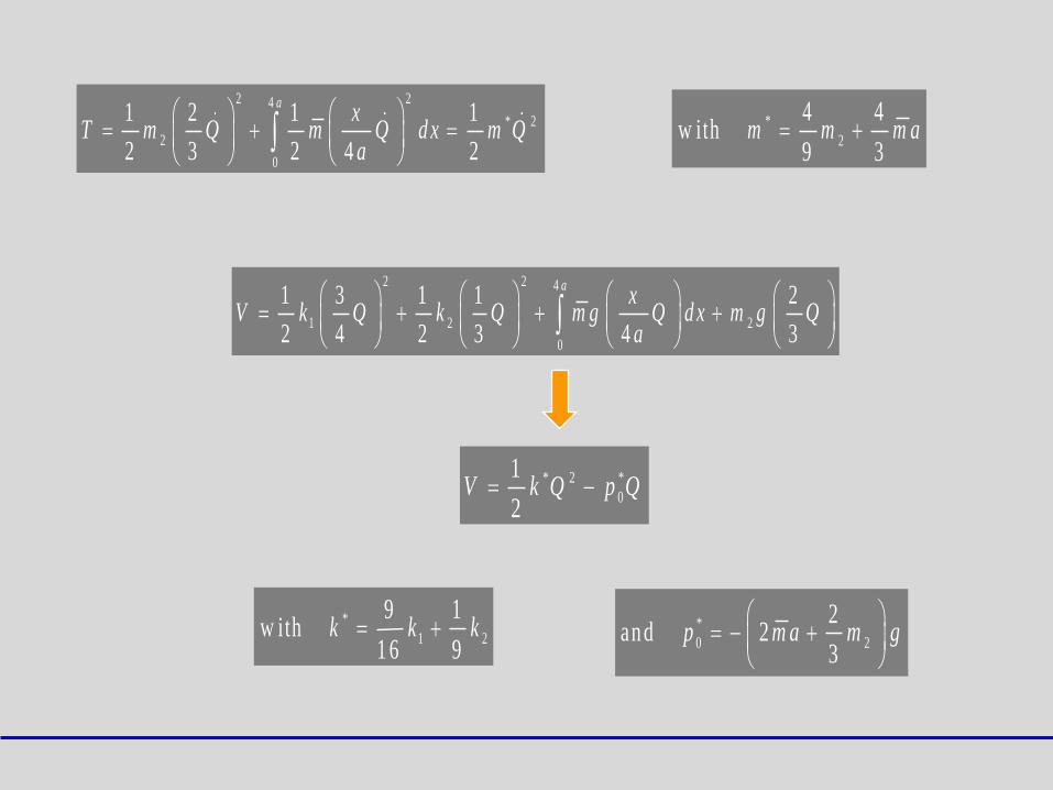
2 24
* 2
2
0
1 2 1 1
2 3 2 4 2
ax
T m Q m Q d x m Qa
*
2
4 4w ith
9 3m m m a
2 2 4
1 2 2
0
1 3 1 1 2
2 4 2 3 4 3
ax
V k Q k Q m g Q d x m g Qa
* 2 *
0
1
2V k Q p Q
*
1 2
9 1w ith
1 6 9k k k *
0 2
2an d 2
3p m a m g
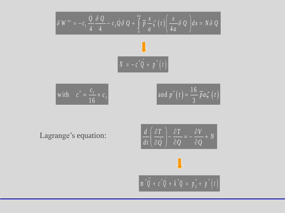
Lagrange’s equation:
4
1 2
04 4 4
a
n c Q Q x xW c c Q Q p t Q d x N Q
a a
* *N c Q p t
* 12w ith
1 6
cc c * 1 6
an d 3
p t p a t
d T T VN
dt Q QQ
* * * * *
0m Q c Q k Q p p t
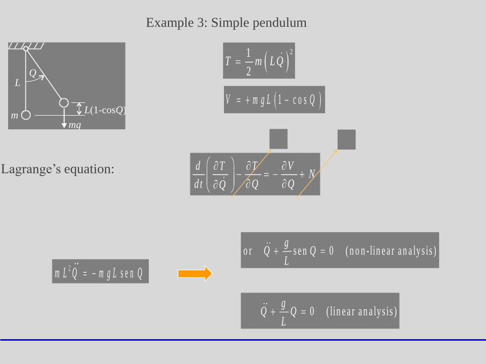
Example 3: Simple pendulum
d T T VN
dt Q QQ
Lagrange’s equation:
21
2T m L Q
1 c o sV m g L Q m
Q
mg
L - Q(1 cos )
L
2 s e nm L Q m g L Q
o r s e n 0 ( n o n -lin e a r a n a ly s is )g
Q QL
0 ( lin e a r a n a lys is )g
Q QL
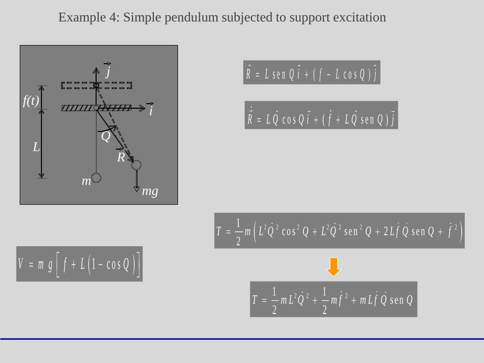
Example 4: Simple pendulum subjected to support excitation
2 2 2 2 2 2 21c o s s e n 2 s e n
2T m L Q Q L Q Q L f Q Q f
1 c o sV m g f L Q
s e n ( c o s )R L Q i f L Q j
c o s ( s e n )R L Q Q i f L Q Q j
2 2 21 1s e n
2 2T m L Q m f m L f Q Q
m
Q
mg
L
f(t)
j
i
R
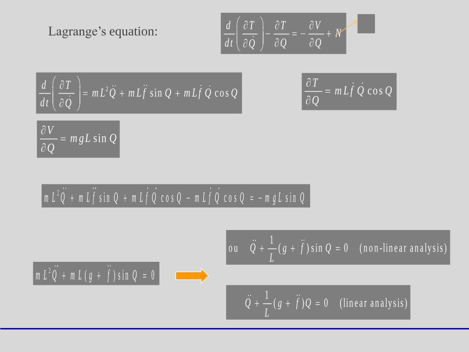
d T T VN
dt Q QQ
Lagrange’s equation:
2 ( ) s i n 0m L Q m L g f Q
1o u ( ) s in 0 ( n o n -lin e a r a n a ly s is )Q g f Q
L
2 s in co sd T
m L Q m L f Q m L f Q Qd t Q
co sT
m L f Q QQ
sinV
m gL QQ
2 s i n c o s c o s s i nm L Q m L f Q m L f Q Q m L f Q Q m g L Q
1 ( ) 0 ( lin e a r a n a ly s is )Q g f Q
L
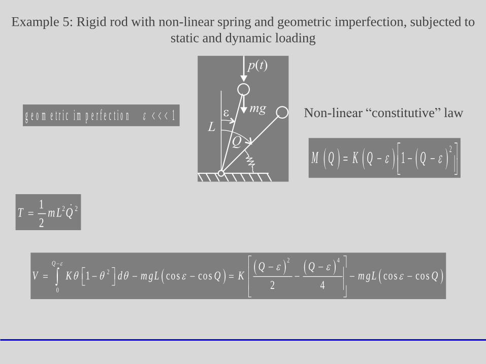
Example 5: Rigid rod with non-linear spring and geometric imperfection, subjected to
static and dynamic loading
Non-linear “constitutive” lawg e o m e t r i c i m p e r f e c t i o n 1
2
1M Q K Q Q
2 21
2T m L Q
2 4
2
0
1 cos cos cos cos2 4
Q Q QV K d m gL Q K m gL Q
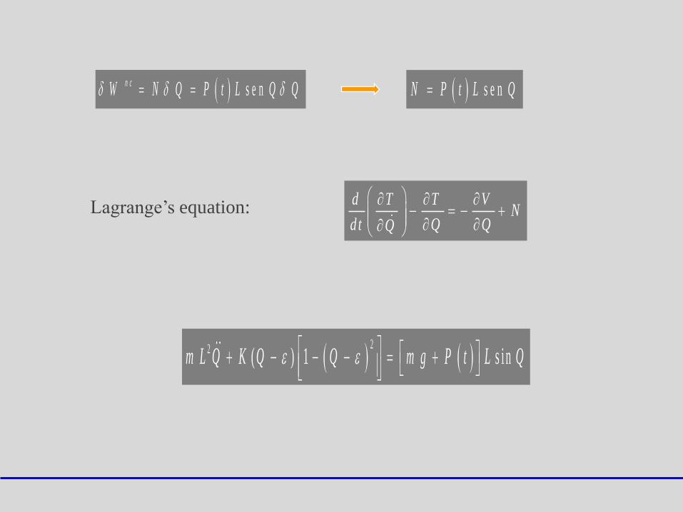
d T T VN
dt Q QQ
Lagrange’s equation:
s e nn cW N Q P t L Q Q s e nN P t L Q
22 ( ) 1 s i nm L Q K Q Q m g P t L Q
Related Documents