Dimensional Testing for Multi-step Similarity Search

Dimensional Testing for Multi-Step Similarity Search

Michael E. Houle∗, Xiguo Ma†, Michael Nett§∗ and Vincent Oria†∗ National Institute of Informatics, Tokyo 101-8430, Japan

Email: {meh, nett}@nii.ac.jp† New Jersey Institute of Technology, Newark, NJ 07102, USA

Email: {xm23, oria}@njit.edu§ University of Tokyo, Tokyo 113-8656, Japan

Abstract—In data mining applications such as subspace clus-tering or feature selection, changes to the underlying featureset can require the reconstruction of search indices to supportfundamental data mining tasks. For such situations, multi-stepsearch approaches have been proposed that can accommodatechanges in the underlying similarity measure without the needto rebuild the index. In this paper, we present a heuristicmulti-step search algorithm that utilizes a measure of intrinsicdimension, the generalized expansion dimension (GED), as thebasis of its search termination condition. Compared to the cur-rent state-of-the-art method, experimental results show that ourheuristic approach is able to obtain significant improvementsin both the number of candidates and the running time, whilelosing very little in the accuracy of the query results.

Keywords-Similarity search; k-NN; nearest neighbor; intrin-sic dimensionality; multi-step; adaptive similarity

I. INTRODUCTION

One of the most fundamental operations employed in data

mining tasks such as classification, cluster analysis, and

anomaly detection, is that of similarity search. Similarity

search is the basis of k-nearest-neighbor (k-NN) classifica-

tion, which often produces the lowest error rates in practice,

particularly when the number of classes is large [1]. For

clustering, many of the most popular strategies require the

determination of neighbor sets based at a large proportion

of the data set objects [1]. Content-based filtering methods

for recommender systems [2] and anomaly detection meth-

ods [3] commonly make use of k-NN techniques, either

through the direct use of k-NN search, or by means of k-NN

cluster analysis. A popular density-based measure, the Local

Outlier Factor (LOF), relies heavily on k-NN computation

to determine the relative density of the data in the vicinity of

the test point [4]. Similarity queries are of two main types:

range queries and k-nearest neighbor (k-NN) queries. Of the

two types of similarity queries, k-NN queries are arguably

more important for data mining applications, perhaps due to

the difficulty faced by the user in deciding range thresholds.

In this paper, we focus on the k-NN search problem.

Traditional indices for similarity search require that the

distance functions used to rank query results be fixed.

In other words, they do not allow distance measures to

be determined adaptively, at query time. In data mining

applications such as subspace clustering or feature selec-

tion, changes to the underlying feature set can require the

reconstruction of search indices to support fundamental data

mining tasks. For such situations, adaptive search approaches

have been proposed that can accommodate changes in the

underlying similarity measure without the need to rebuild the

index [5]. The efficient handling of queries with respect to

adaptive similarity measures can accelerate wrapper methods

for feature selection [6], by accommodating small changes

in the feature set (hopefully) without the need to rebuild

the search indices associated with the feature evaluation

process (such as k-NN classification or clustering). Subspace

clustering [7] is another area that can potentially benefit

from the availability of adaptive similarity indexing, as

cluster formation is generally assessed with respect to a

subset of the features. The effectiveness of using adaptive

(or user-defined) similarity measures have already been

demonstrated for problems with data mining applications,

including content-based image retrieval [8] and document

clustering [9]. In this paper, we will be concerned only with

search methods that can adapt to changes in the underlying

similarity measure or feature set.

To handle adaptive queries, so-called ‘multi-step’ k-NN

strategies have been devised, by which a query result

computed using a fixed ‘lower-bounding’ distance function

can be adapted to answer the same query with respect

to a user-supplied ‘target’ distance function. Formally, d ′

is a lower-bounding distance function for the target d if

d ′(u, v) ≤ d(u, v) for any two objects u, v ∈ U , where Uis a data domain upon which both d ′ and d are defined. Such

lower-bounding relationships arise naturally, for example,

when projecting high-dimensional feature vectors to low-

dimensional feature vectors in Euclidean spaces. In other

cases, d ′ can be a lower-bounding approximation that is

more efficient to compute than d. Lower-bounding distances

that have appeared in the research literature include:

• The lower bound for the max-morphological distance

of 2D shapes [10].

• The 3D-averaging lower bound [11] and the Lp-norm-

based lower bound [12] for the earth mover’s distance.

• The lower bounds for the dynamic time-warping dis-

2012 IEEE 12th International Conference on Data Mining

1550-4786/12 $26.00 © 2012 IEEE

DOI 10.1109/ICDM.2012.91

595

2012 IEEE 12th International Conference on Data Mining

1550-4786/12 $26.00 © 2012 IEEE

DOI 10.1109/ICDM.2012.91

299

tance for time-series data [13].

• The L2-based lower bound for the class of quadratic

form distance functions [14].

In multi-step k-NN search, there are two main stages:

filtering and refinement. In the filtering stage, from the data

set S, a candidate set is generated using d ′. In the refinement

stage, the candidate set is refined using d to get the query

result. Seidl and Kriegel [5] developed an algorithm which

is known to filter the minimum number of candidates needed

in order to guarantee a correct query result after refinement.

Nevertheless, as we will show later, the Seidl-Kriegel (SK)

algorithm may still produce a very large candidate set.

Motivated by this observation, we propose a heuristic

multi-step k-NN search algorithm, that utilizes a general-

ization of a measure of the intrinsic dimensionality of the

data, the expansion dimension [15], [16], as the basis of

an early termination condition. In contrast with previous

multi-step algorithms, we consider a generalization of the

lower-bounding relationship between d ′ and d, in which

λ · d ′(u, v) ≤ d(u, v) for any two objects u, v ∈ U ,

given some lower-bounding ratio λ ≥ 1. The motivation for

introducing λ is to allow as tight as possible a fit between

the lower-bounding distance and the target distance.

The main contributions of this paper are:

• An adaptation of the expansion dimension that allows

the estimation of intrinsic dimension in the vicinity of

a query point q, through the observation of the query

ranks and distances of two neighbors of q, utilized

dynamically to guide the search decisions.

• A novel multi-step algorithm for approximate similarity

search, in which tests of (generalized) expansion di-

mension are used to guide early termination decisions.

• A theoretical analysis of our approach that shows con-

ditions under which an exact result can be guaranteed.

The remainder of this paper is organized as follows. Sec-

tion II discusses previous multi-step algorithms. Section III

provides a formal definition of the generalized expansiondimension, as well as other concepts and terminology that

we require. Section IV presents our proposed algorithm, as

well as its analysis. Experimental results are presented in

Section V. The discussion is concluded in Section VI.

II. MULTI-STEP SEARCH ALGORITHMS

A. Related Work

Adaptive similarity search is loosely related to search

techniques that make use of projection, in that the under-

lying feature space (and therefore the similarity measure)

has been changed. One example of this is the MedScoretechnique, due to Andoni et al. [17], in which the original

high-dimensional feature space is transformed into a low-

dimensional feature space by means of random projections.

For each dimension in the new feature space, a sorted list

is created. The search is done by aggregating precomputed

Algorithm SK (query q, neighborhood size k)

1: Assume there is an index I ′ created with respect to d ′, togetherwith a method getnext that uses I ′ to iterate through the nearestneighbor list of q.

2: Let P be a set of pairs with the form (v, β), where v is anobject and β = d(q, v).

3: P ← ∅.4: dmax ← ∞.5: repeat6: (v, β ′)← I ′.getnext. // β ′ = d ′(q, v)7: if β ′ ≥ dmax then8: Return P.9: end if

10: Compute the target distance value d(q, v).11: P ← P ∪ {(v, d(q, v))}.12: if |P| < k then13: Continue to Line 6.14: else if |P| > k then15: Delete the pair with the largest distance β from P. Ties

are broken arbitrarily.16: end if17: Update the value of dmax to be the largest distance value β

in P.18: until no more objects to be retrieved from I ′.19: Return P.

Figure 1. The multi-step algorithm proposed by Seidl and Kriegel [5].

sorted lists to find the objects with the minimum median

scores. The well-known threshold algorithm [18] is used

here for the aggregation.

The first true lower-bounding (‘multi-step’) k-NN search

algorithm was proposed by Korn et al. [10]. In the filtering

stage, the algorithm first obtains from the data set S the k-

nearest neighbors of q with respect to d ′, and then computes

their distances to q with respect to the target distance d.

From among the target distance values, the maximum value

dmax is determined. The candidate set is then obtained from

S by performing a range query with respect to d ′, where

dmax is used as the range limit. In the refinement stage,

the algorithm simply evaluates the target distances from q

to all the candidates to get the query result. The algorithm

guarantees a correct query result; however, the candidate set

produced may be prohibitively large.

Seidl and Kriegel [5] later proposed a more efficient

multi-step k-NN search algorithm. They showed that their

algorithm is optimal, in the sense that it produces the

minimum number of candidates needed in order to guarantee

a correct query result, based on the information available

given d ′. In other words, with even one such candidate

missing, the query result may not be guaranteed correct. We

will discuss this algorithm in detail in the next subsection.

B. Seidl and Kriegel’s Algorithm

In the remainder of this paper, we will refer to the

algorithm proposed by Seidl and Kriegel [5] as SK. The

description of Algorithm SK is presented in Figure 1. In

contrast to the first multi-step k-NN search algorithm, SK

596300

0.1

0.12

0.14

0.16

0.18

0.2

0.22

1 20 40 60 80Exa

ct a

nd lo

wer

-bou

ndin

g di

stan

ce

Ranking according to lower-bounding distance

Lower-bounding distanceExact distance

Figure 2. An example of a typical 10-NN query on the data set ALOI.The 10-th smallest exact distance is marked by the horizontal line. Inthis example, Algorithm SK produces 64 candidates, although the correctneighbor set is available once the 17th candidate has been produced (asmarked by red circles).

performs rounds of filtering and refinement on a candidate

set that grows incrementally. The function getnext allows for

incremental generation of the neighbors of q with respect to

d ′. An existing method designed for general spatial indices

with such purpose can be found in [19].

At every iteration of the main loop of Algorithm SK, the

candidate set is the current neighborhood of q with respect to

d ′. From the candidate set, the k-nearest neighbors of q with

respect to d are stored as a tentative query result (the set of

object-distance pairs P), and the k-th smallest target distance

is maintained (dmax). The algorithm terminates when the

value of dmax is no greater than the largest lower-bounding

distance that has been seen so far (β ′), or when all the

objects in the data set S have been fetched as candidates and

refined. In [5], Seidl and Kriegel showed that at termination,

the value of dmax will have been decreased to the exact k-th

smallest distance from q to the objects in S, ensuring the

optimality of the algorithm.

Though SK produces only those candidates which are

necessary to obtain an exact query result, it may still

produce an unsatisfactorily large candidate set if the lower-

bounding distance function d ′ used for filtering is not a good

approximation of the exact distance function d.

In Figure 2, we illustrate how Algorithm SK handles a

typical 10-NN query on a real data set, the Amsterdam

Library of Object Images (ALOI) data set described in

Section V. For the example, we projected the original 641-

dimensional feature space to a 20-dimensional feature space,

and used the Euclidean distance on these respective spaces

as the target and lower-bounding distance measures. The

10-th smallest target distance is 0.172, which is marked by

the horizontal line in the figure. To find a lower-bounding

distance no less than 0.172 (thereby reaching one of the two

termination conditions), Algorithm SK must produce and

refine 64 candidates. All these candidates must be verified

in order to guarantee that a correct query result is returned.

Clearly, if one is willing to accept a query result that is

not necessarily exact, the potential exists for improving the

performance of SK by reducing the number of candidates

through early termination.

III. EXPANSION DIMENSION

In this section, we introduce the generalized expansiondimension (GED), which will serve as the basis of the early

termination test used by our proposed multi-step similarity

search heuristic. More details on the GED, including for-

mulations for Lp distances, cosine similarity and Hamming

distances, can be found in [16].

A. Background

In [15], Karger and Ruhl introduced a measure of intrinsic

dimension as a means of analyzing the performance of a

local search strategy for handling nearest neighbor queries.

The complexity of their method depends heavily on the rate

at which the number of visited elements grows as the search

expands. Accordingly, they limited their attention to sets

which satisfied the following smooth-growth property. Let

BS(q, r) = {v ∈ S | d(q, v) ≤ r} be the set of elements of

S ⊆ U contained in the closed ball of radius r centered at

q ∈ U , where U is a data domain. S is said to have (b, α)-expansion if for all q ∈ U and r > 0,

|BS(q, r)| ≥ b =⇒ |BS(q, 2r)| ≤ α · |BS(q, r)| .

The expansion rate of S is the minimum value of α such that

the above condition holds, subject to the choice of minimum

ball size b (in their analysis, Karger and Ruhl chose b =O(log |S|)).

One can consider the value log2 α to be a measure of

the intrinsic dimension, by observing that for the Euclidean

distance metric in Rc, doubling the radius of a sphere

increases its volume by a factor of 2c. When sampling Rc

by a uniformly distributed point set, the expanded sphere

would contain proportionally as many points. Accordingly,

the value of log2 α is often referred to as the expansiondimension of the set. It should be noted that this doubling

property is true of many other distance measures as well,

including the Lp norms. For other norms, the dependence

on c may be different; one such example is the vector angle

distance metric (equivalent to the cosine similarity measure),

where the volume increases by a factor of 2c−1. Although

the definition of expansion dimension can be extended to

handle such distance metrics [16], for simplicity we will

consider only distance metrics (such as weighted Lp norms)

for which doubling the radius of a sphere would increase

the volume by a factor of 2c.

B. Generalized Expansion Dimension

The original definition of expansion rate was motivated

to support analysis that depend on the use of the triangle

inequality. In these contexts, it is useful to consider the effect

of a doubling of the radius of the bounding balls. In general,

however, the dimensionality of the space is revealed by any

two balls of differing radii. Let B1 and B2 be two balls with

the same center q and unequal radii r1 �= r2. If V1 and V2

597301

Generalized expansion dimension:

GED(B≤S (q, r1), B≤

S (q, r2)) =log |B

≤S (q, r2)| − log |B

≤S (q, r1)|

log r2 − log r1.

Inner ball set:

B(q, k) = {B≤S (q, δS(q, j)) | 1 ≤ j ≤ k − 1, δS(q, j) > 0} \ {B

≤S (q, δS(q, k))}.

Maximum expansion dimension:MaxGED(q, k) = max{GED(B, B

≤S (q, δS(q, k))) | B ∈ B(q, k)}.

q

r1r2

B≤

S(q, r1)

B≤

S(q, r2)

Figure 3. Formal definitions of generalized expansion dimension and maximum expansion dimension.

are the respective volumes of B1 and B2, then the dimension

of the set is given by

rDim =log V2 − log V1

log r2 − log r1.

Accordingly, by estimating the spherical volumes V1 and

V2 by the numbers of data points they contain (call them

k1 and k2), we can estimate the dimensionality of the data

set in the vicinity of B1 and B2 by:

GED(B1, B2) =log k2 − log k1

log r2 − log r1.

The balls B1 and B2 constitute two lower-dimensional

measurements — distance-rank pairs — that together allow

an assessment of the higher-dimensional structure — the

intrinsic dimension — of the data points in the vicinity of

the balls. We refer to GED(B1, B2) as a dimensional testvalue from the perspective of B1 and B2. Changing B1

or B2 would likely produce a change in the result of the

dimensional test; however, aggregating the results of such

tests over a range of ball radii or sizes can produce a useful

estimate of the overall intrinsic dimension in the vicinity of

a query point.

In order to provide formal definitions of generalized mea-

sures of the expansion dimension, we first require additional

terminology and notation. For a point q ∈ U and a data

set X ⊆ U , let νX(q, k) be the k-th nearest neighbor of q

in X with respect to d. Ties in distance values are broken

arbitrarily but consistently. Let δX(q, k) = d(q, νX(q, k))be the distance from q to its k-th nearest neighbor. Given

a point q ∈ U and a radius r > 0, we denote by B≤S (q, r)

the closed ball centered at q with radius r containing all

the points v ∈ S satisfying d(q, v) ≤ r, and B<S (q, r) the

open ball centered at q with radius r containing all the

points v ∈ S satisfying d(q, v) < r. Let |B≤S (q, r)| and

|B<S (q, r)| denote the numbers of points of S contained in

the two balls B≤S (q, r) and B<

S (q, r), respectively. Given two

closed balls B≤S (q, r1) and B

≤S (q, r2) with radii 0 < r1 < r2

and the numbers of points of S contained in them satisfying

0 < |B≤S (q, r1)| < |B

≤S (q, r2)|, the generalized expansion

dimension is defined as in Figure 3. We also define the innerball set and the maximum expansion dimension (MED) rela-

tive to a point q ∈ U and a neighborhood size k ≥ 2, again

in Figure 3. Note that MaxGED(q, k) would be undefined if

the inner ball set B(q, k) is empty. In other words, in order

for MaxGED(q, k) to be properly defined, there must be at

least one ball B≤S (q, δS(q, j)), where 1 ≤ j ≤ k − 1, with

radius satisfying 0 < δS(q, j) < δS(q, k).In the past, measures of intrinsic dimension (such as

the expansion dimension) have been used strictly for the

analysis of similarity search methods. In the next section, we

demonstrate that tests of (generalized) expansion dimension

can be used to dynamically guide the decisions made by

search algorithms.

IV. ALGORITHM

We now turn our attention to the main contribution of the

paper, Algorithm MAET (Multi-step Algorithm with Early

Termination). Let us first introduce some needed notations.

For a query q ∈ U and a data set X ⊆ U , let NX(q, k) be

the set of k-nearest neighbors of q over X, with respect to

d. Ties are broken arbitrarily and consistently. Let R≤X(q, r)

be the closed range set of objects in X having distances to

q (with respect to d) no greater than r, and R<X (q, r) be the

open range set of objects in X having distances to q (with

respect to d) strictly less than r.

A. Algorithm MAETAlgorithm MAET is described in Figure 4. The algorithm

accepts a query q ∈ U , a target query result size k > 0, a

lower-bounding ratio λ ≥ 1, and a termination parameter t >

0 as its inputs. Throughout the search process, the algorithm

maintains a tentative query result set P. At each iteration,

the algorithm obtains a candidate object from the underlying

index structure I ′, computes its exact distance to q, and

stores in the result set P those k objects associated with

the smallest distances encountered so far. After at least k

candidates have been retrieved and stored in P, two closed

balls centered at q are determined. The inner ball contains

at least k1 > 0 points of S and has r1 > 0 as its radius; the

outer ball contains at least k > 0 points of S and has r > 0 as

its radius. Provided that the two balls are distinct (k1 �= k),

a dimensional test is performed. If the test indicates that a

termination condition has been reached (as determined by

termination parameter t), the algorithm halts and returns P.

In the next subsection, we will show that when k1 > 0 and

k1 �= k hold, k1 < k and r1 < r must hold, and the inner

ball contains exactly k1 points of S.

598302

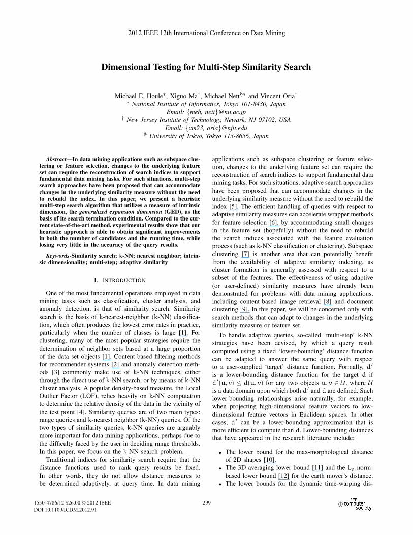
Algorithm MAET (query q, neighborhood size k, lower-boundingratio λ, termination parameter t)

1: Assume there is an index I ′ created with respect to d ′, togetherwith a method getnext that uses I ′ to iterate through the nearestneighbor list of q.

2: Let P be a set of pairs with the form (v, β), where v is an objectand β = d(q, v). Let Pv denote the object set associated withP.

3: P ← ∅.4: repeat5: (v, β ′)← I ′.getnext. // β ′ = d ′(q, v)6: Compute the target distance value from q to v, d(q, v).7: P ← P ∪ {(v, d(q, v))}.8: if |P| < k then9: Continue to Line 5.

10: else if |P| > k then11: Delete the pair with the largest distance β from P. Ties

are broken arbitrarily.12: end if13: k1 ← |R<

Pv(q, λ · β ′)|.

14: if k1 = k then15: Return P.16: else if k1 > 0 then17: r← δPv(q, k).18: r1 ← δPv(q, k1).19: if r1 > 0 and k1 · (r/r1)t < k + 1 then20: Return P.21: end if22: end if23: until no more objects to be retrieved from I ′.24: Return P.

Figure 4. The description of Algorithm MAET.

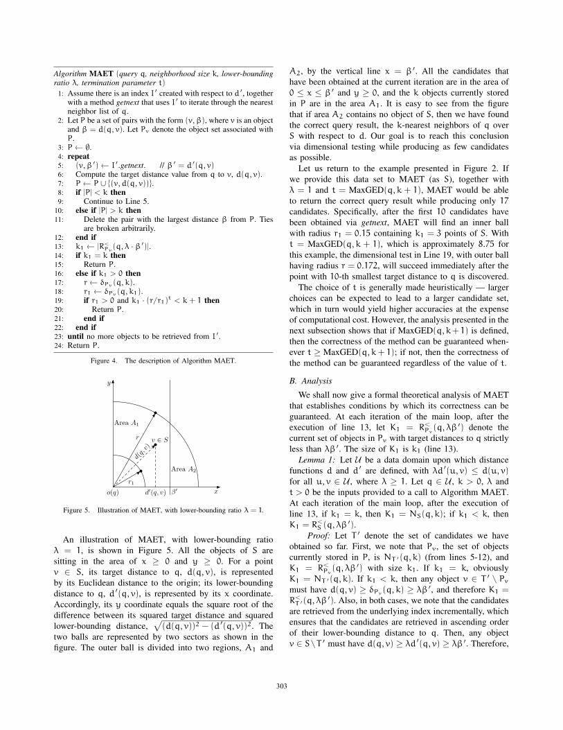
d(q,v)

d′(q, v)

v ∈ S

x

y

r

r1

β′o(q)

Area A1

Area A2

Figure 5. Illustration of MAET, with lower-bounding ratio λ = 1.

An illustration of MAET, with lower-bounding ratio

λ = 1, is shown in Figure 5. All the objects of S are

sitting in the area of x ≥ 0 and y ≥ 0. For a point

v ∈ S, its target distance to q, d(q, v), is represented

by its Euclidean distance to the origin; its lower-bounding

distance to q, d ′(q, v), is represented by its x coordinate.

Accordingly, its y coordinate equals the square root of the

difference between its squared target distance and squared

lower-bounding distance,√

(d(q, v))2 − (d ′(q, v))2. The

two balls are represented by two sectors as shown in the

figure. The outer ball is divided into two regions, A1 and

A2, by the vertical line x = β ′. All the candidates that

have been obtained at the current iteration are in the area of

0 ≤ x ≤ β ′ and y ≥ 0, and the k objects currently stored

in P are in the area A1. It is easy to see from the figure

that if area A2 contains no object of S, then we have found

the correct query result, the k-nearest neighbors of q over

S with respect to d. Our goal is to reach this conclusion

via dimensional testing while producing as few candidates

as possible.

Let us return to the example presented in Figure 2. If

we provide this data set to MAET (as S), together with

λ = 1 and t = MaxGED(q, k + 1), MAET would be able

to return the correct query result while producing only 17

candidates. Specifically, after the first 10 candidates have

been obtained via getnext, MAET will find an inner ball

with radius r1 = 0.15 containing k1 = 3 points of S. With

t = MaxGED(q, k + 1), which is approximately 8.75 for

this example, the dimensional test in Line 19, with outer ball

having radius r = 0.172, will succeed immediately after the

point with 10-th smallest target distance to q is discovered.

The choice of t is generally made heuristically — larger

choices can be expected to lead to a larger candidate set,

which in turn would yield higher accuracies at the expense

of computational cost. However, the analysis presented in the

next subsection shows that if MaxGED(q, k+ 1) is defined,

then the correctness of the method can be guaranteed when-

ever t ≥ MaxGED(q, k + 1); if not, then the correctness of

the method can be guaranteed regardless of the value of t.

B. Analysis

We shall now give a formal theoretical analysis of MAET

that establishes conditions by which its correctness can be

guaranteed. At each iteration of the main loop, after the

execution of line 13, let K1 = R<Pv

(q, λβ ′) denote the

current set of objects in Pv with target distances to q strictly

less than λβ ′. The size of K1 is k1 (line 13).

Lemma 1: Let U be a data domain upon which distance

functions d and d ′ are defined, with λd ′(u, v) ≤ d(u, v)for all u, v ∈ U , where λ ≥ 1. Let q ∈ U , k > 0, λ and

t > 0 be the inputs provided to a call to Algorithm MAET.

At each iteration of the main loop, after the execution of

line 13, if k1 = k, then K1 = NS(q, k); if k1 < k, then

K1 = R<S (q, λβ ′).

Proof: Let T ′ denote the set of candidates we have

obtained so far. First, we note that Pv, the set of objects

currently stored in P, is NT ′(q, k) (from lines 5-12), and

K1 = R<Pv

(q, λβ ′) with size k1. If k1 = k, obviously

K1 = NT ′(q, k). If k1 < k, then any object v ∈ T ′ \ Pv

must have d(q, v) ≥ δPv(q, k) ≥ λβ ′, and therefore K1 =R<

T ′(q, λβ ′). Also, in both cases, we note that the candidates

are retrieved from the underlying index incrementally, which

ensures that the candidates are retrieved in ascending order

of their lower-bounding distance to q. Then, any object

v ∈ S\T ′ must have d(q, v) ≥ λd ′(q, v) ≥ λβ ′. Therefore,

599303

if k1 = k, then K1 = NS(q, k) must be true; if k1 < k,

then K1 = R<S (q, λβ ′) must be true.

Theorem 1: Let U be a data domain upon which distance

functions d and d ′ are defined, with λd ′(u, v) ≤ d(u, v)for all u, v ∈ U where λ ≥ 1. Let q ∈ U , k > 0, λ and

t > 0 be the inputs provided to a call to Algorithm MAET.

If MaxGED(q, k + 1) is defined, then the algorithm returns

the correct query result whenever t ≥ MaxGED(q, k + 1).Otherwise, the algorithm returns the correct query result

regardless of the value of t.

Proof: First, we note that the algorithm must terminate,

as the iterative retrieval of candidates would eventually result

in the termination condition of the loop being reached (Line

23). In this case, all the target distance values from q to

every object in S would have been evaluated, and only the

k objects with the smallest distances would have been stored

in P (Lines 5-12). Obviously, the algorithm would return the

correct result for this case.

Otherwise, the algorithm would terminate with one of the

following two conditions being reached (Line 14 or 19):

k1 = k or

k1

(r

r1

)t

< k + 1. (1)

For the case when k1 = k, K1 = NS(q, k) must be true

(from Lemma 1). By the definitions of K1 and Pv, we know

that all the objects in K1 are currently stored in P. Also, we

have |P| = k. Therefore, the algorithm returns the correct

result for this case also.

For the last case when Inequality (1) holds, r1 > 0, k1 >

0 and k1 �= k must be true (Lines 19 and 16). Together

with k1 = |R<Pv

(q, λβ ′)| ≤ |Pv| = k, we obtain k1 < k

for this case. Since |R<Pv

(q, λβ ′)| = k1 < k, we have r1 =δPv(q, k1) < λβ ′ and r = δPv(q, k) ≥ λβ ′. Consequently,

r1 < r must be true for this case. From Lemma 1, we know

that K1 = R<S (q, λβ ′). Together with K1 = R<

Pv(q, λβ ′)

and |K1| = k1, we can derive

r1 = δPv(q, k1) = δK1(q, k1) = δS(q, k1) < δS(q, k1+1).

Therefore, the closed ball B≤S (q, δS(q, k1)) has r1 as its

radius and contains exactly k1 points of S. We also know

that the closed ball B≤S (q, δS(q, k + 1)) has δS(q, k + 1)

as its radius and contains |B≤S (q, δS(q, k + 1))| points of S.

Since k1 < k, we obtain r1 < δS(q, k1 +1) ≤ δS(q, k+1).Thus, MaxGED(q, k + 1) is defined for this case. Assume

t ≥ MaxGED(q, k + 1), we can derive

k1

(δS(q, k + 1)

r1

)t

≥ |B≤S (q, δS(q, k + 1))| ≥ k + 1.

Together with Inequality (1), r < δS(q, k + 1) must hold

for this case. Also, we have |P| = k and r = δPv(q, k), so

all the k objects in P have target distances to q less than

δS(q, k+ 1). Therefore, we can conclude that the algorithm

returns the correct result for the last case.

C. Sampling of Potential Queries

We have shown that for a particular query q ∈ U , if

MaxGED(q, k + 1) is defined, then MAET is guaranteed to

produce a correct k-NN query result whenever termination

parameter t ≥ MaxGED(q, k+1); otherwise, MAET returns

the correct query result regardless of the value of t. In

this subsection, we further show how that t can be chosen

through sampling of potential queries for MAET, in order

to correctly answer a desired proportion of potential queries

with high probability. We will first describe the method

for determining such a value of t, and then justify the

method by providing a technical lemma. We call this method

SamplingGED.

Let D(U) be a list of |U | real values. For each point q ∈U , a value a = MaxGED(q, k + 1) exists in list D(U).If MaxGED(q, k + 1) is undefined, a = −1. The method

SamplingGED can be stated as follows:

1. Sample a set U1 uniformly at random without replace-

ment from U .

2. Compute list D(U1).3. Choose termination parameter t > 0 to be the smallest

value for which at least a desired proportion 0 < η1 ≤ 1

of the list entries D(U1) are no greater than t.

Correspondingly, we let η denote the proportion of values in

D(U) which are no greater than t. According to Theorem 1,

if we provide this choice of t to MAET, the proportion of

queries in U (and U1) for which MAET is guaranteed to

answer correctly is η (and η1 respectively). Now, we shall

establish the relationship between the true success rate η and

the sample success rate η1.

Lemma 2: Let N be a list of n real numbers and let

N1 be a list of n1 elements sampled uniformly at random

from list N without replacement. Given a threshold t ∈ R,

let m and m1 refer to the number of elements in N and

N1, respectively, that are no greater than t. Take η and

η1 to refer to the proportion of those elements within N

and N1, respectively. For any real number φ ≥ 0, we have

Pr[|η1 − η| ≥ φ] ≤ 2e−2φ2n1 .

Proof: Omitted in this version; see [16] for details.

When taking N = D(U) and N1 = D(U1), Lemma 2

states that the probability of the unknown success rate η

deviating from the sample success rate η1 by more than

φ ≥ 0 is at most 2e−2φ2|U1|. That is, the probability of

the true success rate being significantly less than the sample

success rate vanishes as the sample size grows. Therefore,

for a reasonable value of φ ≥ 0, we are able to choose a

global value of t (through method SamplingGED) for MAET

to correctly answer a certain proportion (η1−φ) of potential

queries with high probability.

As an illustrative example, let us suppose that in Step 1 of

SamplingGED we sample a set U1 with size |U1| = 1000,

and then determine a value of t in Step 3 by choosing a

desired success rate η1 = 95% for this sample. Then the

600304

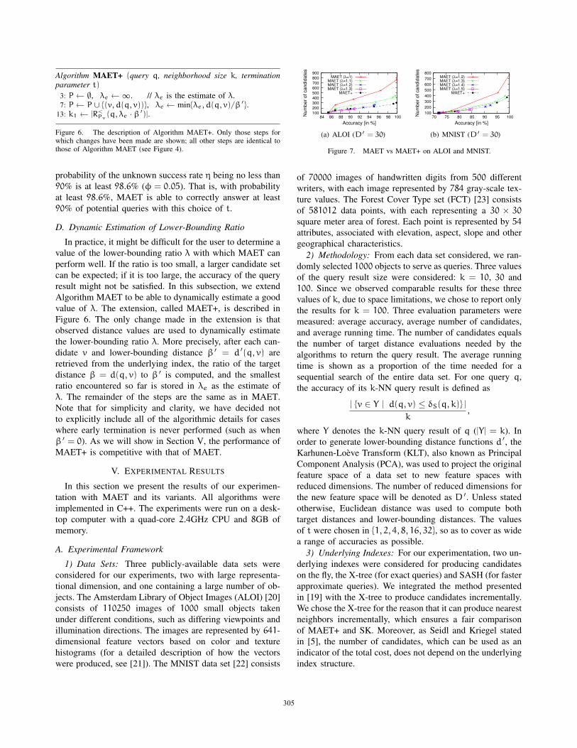
Algorithm MAET+ (query q, neighborhood size k, terminationparameter t)

3: P ← ∅, λe ← ∞. // λe is the estimate of λ.7: P ← P ∪ {(v, d(q, v))}, λe ← min{λe , d(q, v)/β ′}.

13: k1 ← |R<Pv

(q, λe · β ′)|.

Figure 6. The description of Algorithm MAET+. Only those steps forwhich changes have been made are shown; all other steps are identical tothose of Algorithm MAET (see Figure 4).

probability of the unknown success rate η being no less than

90% is at least 98.6% (φ = 0.05). That is, with probability

at least 98.6%, MAET is able to correctly answer at least

90% of potential queries with this choice of t.

D. Dynamic Estimation of Lower-Bounding Ratio

In practice, it might be difficult for the user to determine a

value of the lower-bounding ratio λ with which MAET can

perform well. If the ratio is too small, a larger candidate set

can be expected; if it is too large, the accuracy of the query

result might not be satisfied. In this subsection, we extend

Algorithm MAET to be able to dynamically estimate a good

value of λ. The extension, called MAET+, is described in

Figure 6. The only change made in the extension is that

observed distance values are used to dynamically estimate

the lower-bounding ratio λ. More precisely, after each can-

didate v and lower-bounding distance β ′ = d ′(q, v) are

retrieved from the underlying index, the ratio of the target

distance β = d(q, v) to β ′ is computed, and the smallest

ratio encountered so far is stored in λe as the estimate of

λ. The remainder of the steps are the same as in MAET.

Note that for simplicity and clarity, we have decided not

to explicitly include all of the algorithmic details for cases

where early termination is never performed (such as when

β ′ = 0). As we will show in Section V, the performance of

MAET+ is competitive with that of MAET.

V. EXPERIMENTAL RESULTS

In this section we present the results of our experimen-

tation with MAET and its variants. All algorithms were

implemented in C++. The experiments were run on a desk-

top computer with a quad-core 2.4GHz CPU and 8GB of

memory.

A. Experimental Framework

1) Data Sets: Three publicly-available data sets were

considered for our experiments, two with large representa-

tional dimension, and one containing a large number of ob-

jects. The Amsterdam Library of Object Images (ALOI) [20]

consists of 110250 images of 1000 small objects taken

under different conditions, such as differing viewpoints and

illumination directions. The images are represented by 641-

dimensional feature vectors based on color and texture

histograms (for a detailed description of how the vectors

were produced, see [21]). The MNIST data set [22] consists

100 200 300 400 500 600 700 800 900

84 86 88 90 92 94 96 98 100Num

ber

of c

andi

date

s

Accuracy [in %]

MAET (λ=1)MAET (λ=1.1)MAET (λ=1.2)MAET (λ=1.3)

MAET+

(a) ALOI (D′ = 30)

100 200 300 400 500 600 700 800

70 75 80 85 90 95 100Num

ber

of c

andi

date

s

Accuracy [in %]

MAET (λ=1.2)MAET (λ=1.3)MAET (λ=1.4)MAET (λ=1.5)

MAET+

(b) MNIST (D′ = 30)

Figure 7. MAET vs MAET+ on ALOI and MNIST.

of 70000 images of handwritten digits from 500 different

writers, with each image represented by 784 gray-scale tex-

ture values. The Forest Cover Type set (FCT) [23] consists

of 581012 data points, with each representing a 30 × 30

square meter area of forest. Each point is represented by 54

attributes, associated with elevation, aspect, slope and other

geographical characteristics.

2) Methodology: From each data set considered, we ran-

domly selected 1000 objects to serve as queries. Three values

of the query result size were considered: k = 10, 30 and

100. Since we observed comparable results for these three

values of k, due to space limitations, we chose to report only

the results for k = 100. Three evaluation parameters were

measured: average accuracy, average number of candidates,

and average running time. The number of candidates equals

the number of target distance evaluations needed by the

algorithms to return the query result. The average running

time is shown as a proportion of the time needed for a

sequential search of the entire data set. For one query q,

the accuracy of its k-NN query result is defined as

| {v ∈ Y | d(q, v) ≤ δS(q, k)} |

k,

where Y denotes the k-NN query result of q (|Y| = k). In

order to generate lower-bounding distance functions d ′, the

Karhunen-Loeve Transform (KLT), also known as Principal

Component Analysis (PCA), was used to project the original

feature space of a data set to new feature spaces with

reduced dimensions. The number of reduced dimensions for

the new feature space will be denoted as D ′. Unless stated

otherwise, Euclidean distance was used to compute both

target distances and lower-bounding distances. The values

of t were chosen in {1, 2, 4, 8, 16, 32}, so as to cover as wide

a range of accuracies as possible.

3) Underlying Indexes: For our experimentation, two un-

derlying indexes were considered for producing candidates

on the fly, the X-tree (for exact queries) and SASH (for faster

approximate queries). We integrated the method presented

in [19] with the X-tree to produce candidates incrementally.

We chose the X-tree for the reason that it can produce nearest

neighbors incrementally, which ensures a fair comparison

of MAET+ and SK. Moreover, as Seidl and Kriegel stated

in [5], the number of candidates, which can be used as an

indicator of the total cost, does not depend on the underlying

index structure.

601305

100

110

120

130

140

5 10 15 20 25 30Num

ber

of c

andi

date

s

Number of reduced dimensions

MAET+ (t=32)SK

0

4

8

12

16

20

5 10 15 20 25 30

Run

ning

tim

e [in

%]

Number of reduced dimensions

MAET+ (t=32)SK

Figure 8. MAET+ vs SK on FCT (single d). The accuracy of MAET+with t = 32 is more than 99%.

102

103

104

10 20 30 40 50 60Num

ber

of c

andi

date

s

Number of reduced dimensions

MAET+ (t=8)MAET+ (t=16)

SK

4

8

12

16

20

24

10 20 30 40 50 60

Run

ning

tim

e [in

%]

Number of reduced dimensions

MAET+ (t=8)MAET+ (t=16)

SK

Figure 9. MAET+ vs SK on ALOI (single d). The accuracies of MAET+are approximately 93% and 99% for t = 8 and 16, respectively.

102

103

104

105

10 20 30 40 50 60Num

ber

of c

andi

date

s

Number of reduced dimensions

MAET+ (t=16)MAET+ (t=32)

SK

0

10

20

30

40

50

60

10 20 30 40 50 60

Run

ning

tim

e [in

%]

Number of reduced dimensions

MAET+ (t=16)MAET+ (t=32)

SK

Figure 10. MAET+ vs SK on MNIST (single d). The accuracies ofMAET+ are approximately 95% and 99% for t = 16 and 32, respectively.

B. MAET vs MAET+

For the first set of experiments, we compared the perfor-

mance of dynamic estimation of the lower-bounding ratio

λ (MAET+) against that of fixed choices of λ (MAET).

All three data sets were used here. The number of reduced

dimensions D ′ was chosen to be 5, 30 and 30 for FCT,

ALOI and MNIST, respectively. The X-tree was used as an

appropriate underlying index for this set of experiments.

The results are shown in Figure 7. Due to space limita-

tions, the CPU time, which follows almost exactly the same

trend as the number of candidates in this example, is not

shown in this figure. The plot for the FCT experiment is

also not shown, since all methods tested performed virtually

identically. From the results, we can find that MAET+ is

consistently competitive with MAET, which is provided with

several fixed choices of λ. For MAET, the choice of λ that

leads to a given accuracy value is different across the various

data sets. For example, the best values of λ to achieve

95% average accuracy are 1.1, 1.2 and 1.3 for FCT, ALOI

and MNIST, respectively. For this reason, and due to space

limitations, for all the remaining experiments except those

appearing in Section V-E, we omit the experimental results

of MAET, and instead compare only MAET+ with SK.

C. MAET+ vs SK

Two sets of experiments were conducted for comparing

the performance of MAET+ with that of SK. In the first set,

we compared their performances in dealing with one target

102

103

104

75 80 85 90 95 100Num

ber

of c

andi

date

s

Accuracy [in %]

MAET+ (L2)SK (L2)

MAET+ (WL2)SK (WL2)

MAET+ (L1)SK (L1)

0

1

2

3

4

5

75 80 85 90 95 100

Run

ning

tim

e [in

%]

Accuracy [in %]

MAET+ (L2)SK (L2)

MAET+ (WL2)SK (WL2)

MAET+ (L1)SK (L1)

Figure 11. MAET+ vs SK on FCT (adaptive d). D′ = 5.

102

103

104

105

106

70 75 80 85 90 95 100Num

ber

of c

andi

date

s

Accuracy [in %]

MAET+ (L2)SK (L2)

MAET+ (WL2)SK (WL2)

MAET+ (L1)SK (L1)

4

6

8

10

12

14

16

70 75 80 85 90 95 100

Run

ning

tim

e [in

%]

Accuracy [in %]

MAET+ (L2)SK (L2)

MAET+ (WL2)SK (WL2)

MAET+ (L1)

Figure 12. MAET+ vs SK on ALOI (adaptive d). D′ = 20.

101

102

103

104

105

70 75 80 85 90 95 100Num

ber

of c

andi

date

s

Accuracy [in %]

MAET+ (L2)SK (L2)

MAET+ (WL2)SK (WL2)

MAET+ (L1)SK (L1)

10 15 20 25 30 35 40 45

70 75 80 85 90 95 100

Run

ning

tim

e [in

%]

Accuracy [in %]

MAET+ (L2)SK (L2)

MAET+ (WL2)SK (WL2)

MAET+ (L1)

Figure 13. MAET+ vs SK on MNIST (adaptive d). D′ = 40.

distance function d with respect to different lower-bounding

distance functions d ′. In the second set, we compared their

performances in handling adaptive target distance functions

with respect to one lower-bounding distance function. The

X-tree was used for the comparison.

1) Single Target Distance Function: In this set of ex-

periments, MAET+ and SK were compared for one choice

of target distance function, but with several choices of

lower-bounding distance functions. All three data sets were

used for the comparison. For each data set, 6 values for

the number of reduced dimension D ′ were chosen, each

corresponding to a lower-bounding distance function for

which an X-tree was created. The results for FCT, ALOI and

MNIST are displayed in Figure 8, 9 and 10, respectively.

From the results for all three data sets, we can observe

that with the increase of the number of reduced dimensions,

the number of candidates monotonically decreases for both

MAET+ and SK, whereas the running time does not, or

may even monotonically increase. This is due to the effect

of dimensionality on the performance of X-tree indexing.

For the FCT data set, the performances of MAET+

and SK are similar. However, for the other two data sets,

MAET+ shows improvement over SK while sacrificing little

in accuracy, with respect to all choices of lower-bounding

distance functions. The improvement is especially evident

when the number of reduced dimensions is small — that

is, when the lower-bounding distance function is not a very

good approximation of the target distance function.

Comparing the results across the three data sets for a

common value of D ′ (for example, D ′ = 10), we find

that MAET+ obtains the largest improvement over SK on

602306

MNIST; however, on FCT, no improvement is obtained.

This can be explained by differences in the approximation

qualities of d ′ to d across these data sets. Compared to

SK, our method MAET+ is able to make further predictions

of future distances, due to both tests of dimensionality and

the dynamic estimation of lower-bounding ratio. Therefore,

more improvement of MAET+ over SK can be expected as

the approximation quality of d ′ to d worsens.

2) Adaptive Target Distance Functions: In this set of

experiments, we compared the performances of MAET+ and

SK regarding their ability to handle adaptive target distance

functions. Here, all three data sets were used. Three target

distance functions were considered: Euclidean distance (L2),

weighted Euclidean distance (WL2) and Manhattan distance

(L1). Euclidean distance was used for d ′. In order to ensure

the lower-bounding property, every weight used in WL2

was randomly selected uniformly from the range [1, 2]. The

number of reduced dimensions D ′ was chosen to be 5

for FCT, 20 for ALOI, and 40 for MNIST, the values for

which SK achieved its smallest execution times using the

L2 distance. The results are shown in Figure 11, 12 and 13

for FCT, ALOI and MNIST, respectively.

From the results for ALOI and MNIST, we can find that

MAET+ outperforms SK while still maintaining very high

accuracy for all three target distance functions considered.

The improvement is not so evident in the results for FCT.

We note that when handling queries with respect to L1 on

ALOI and MNIST, Algorithm SK completely fails, in that

it must refine almost every object in the data set to get the

correct query result. In contrast, MAET+ still performs well

with respect to both the total cost and the accuracy.

D. Further Evaluation of MAET+

For this set of experiments, we evaluated the performance

of MAET+ using the SASH as the underlying index. Specif-

ically, we tested the performance of MAET+ in handling

adaptive target distance functions with respect to one lower-

bounding distance function. Two data sets were used for the

evaluation, ALOI and MNIST. As FCT is a sparse data set

with only 54 dimensions in total, the X-tree performs very

efficiently for this set, eliminating the need to use a fast ap-

proximate similarity search index such as the SASH; for this

reason, FCT was omitted from this experiment. Three target

distance functions were considered: Euclidean distance (L2),

weighted Euclidean distance (WL2) and Manhattan distance

(L1). For both ALOI and MNIST, the number of reduced

dimensions D ′ was chosen to be 60. Euclidean distance was

used for computing lower-bounding distances. Again, every

weight used in WL2 was randomly selected from the range

[1, 2] to ensure the lower-bounding property. The results are

displayed in Figure 14 for ALOI, and Figure 15 for MNIST.

From the results for both ALOI and MNIST, we observe

that significant speedups (of roughly two order of magni-

tudes) are achieved by MAET+ as compared to sequential

0 200 400 600 800

1000 1200 1400 1600

70 75 80 85 90 95 100Num

ber

of c

andi

date

s

Accuracy [in %]

MAET+ (L2)MAET+ (WL2)

MAET+ (L1)

0 1 2 3 4 5 6 7 8

70 75 80 85 90 95 100

Run

ning

tim

e [in

%]

Accuracy [in %]

MAET+ (L2)MAET+ (WL2)

MAET+ (L1)

Figure 14. The results of MAET+ on ALOI (D′ = 60). SASH wasused as the underlying index structure, with approximately 93% averageaccuracy.

100 150 200 250 300 350 400 450

75 80 85 90 95 100Num

ber

of c

andi

date

s

Accuracy [in %]

MAET+ (L2)MAET+ (WL2)

MAET+ (L1)

0

1

2

3

4

5

75 80 85 90 95 100

Run

ning

tim

e [in

%]

Accuracy [in %]

MAET+ (L2)MAET+ (WL2)

MAET+ (L1)

Figure 15. The results of MAET+ on MNIST (D′ = 60). SASH wasused as the underlying index structure, with approximately 94% averageaccuracy.

search, all while maintaining very high accuracy, for the L2

and WL2 distances. For the L1 distance, MAET+ obtains a

speedup of more than one order of magnitude for both ALOI

and MNIST. Moreover, for all three target distance functions,

the number of candidates never exceeds 1.4% and 0.7% of

the size of ALOI and MNIST, respectively.

E. Theoretical Bounds and Practical Performance

The theoretical analysis in Section IV-C indicates that

through method SamplingGED, we are able to choose

a value of t for MAET to correctly answer a desired

proportion of potential queries with high probability. In

this subsection, we will show that the performance of our

method in practice is considerably better even than what the

theoretical bounds indicate, through a set of experiments on

all three available data sets.

In our experiment, we considered all data objects as

potential queries. The value of k was chosen to be 100.

In order to obtain a lower-bounding distance function, KLT

was used to project the original feature space of each data

set to a lower-dimensional feature space. For all three data

sets, the number of reduced dimensions of the new feature

space was chosen to be 10. Euclidean distance was used

for both the target distance function and the lower-bounding

distance function. In order to avoid the introduction of error

by overestimating the lower-bounding ratio λ, we set λ = 1.

By applying SamplingGED on each data set, we picked 10

values for t, corresponding to 10 desired proportions η1 at

intervals of 0.1, from 0.1 to 1. The sample size was chosen

to be 1000. The X-tree was used as an underlying exact

index structure. For this set of experiments, we measured the

proportion of queries for which MAET returns the correct

query result; this proportion is denoted by θ in the results

displayed in Table I. We also measured the average number

of candidates as an indicator of the total cost needed by

603307

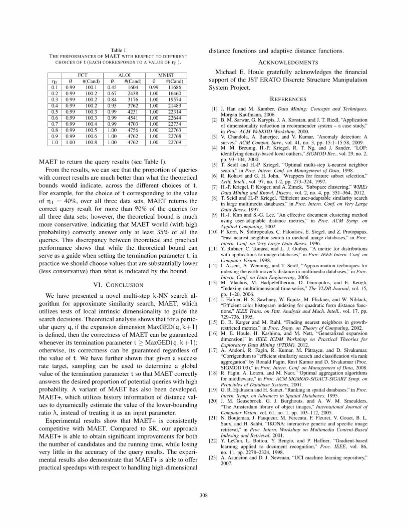
Table ITHE PERFORMANCES OF MAET WITH RESPECT TO DIFFERENT

CHOICES OF t (EACH CORRESPONDS TO A VALUE OF η1 ).

FCT ALOI MNISTη1 θ #(Cand) θ #(Cand) θ #(Cand)0.1 0.99 100.1 0.45 1604 0.99 116860.2 0.99 100.2 0.67 2438 1.00 164600.3 0.99 100.2 0.84 3176 1.00 195740.4 0.99 100.2 0.95 3762 1.00 214890.5 0.99 100.3 0.99 4231 1.00 223140.6 0.99 100.3 0.99 4541 1.00 226440.7 0.99 100.4 0.99 4703 1.00 227340.8 0.99 100.5 1.00 4756 1.00 227630.9 0.99 100.6 1.00 4762 1.00 227681.0 1.00 100.8 1.00 4762 1.00 22769

MAET to return the query results (see Table I).

From the results, we can see that the proportion of queries

with correct results are much better than what the theoretical

bounds would indicate, across the different choices of t.

For example, for the choice of t corresponding to the value

of η1 = 40%, over all three data sets, MAET returns the

correct query result for more than 90% of the queries for

all three data sets; however, the theoretical bound is much

more conservative, indicating that MAET would (with high

probability) correctly answer only at least 35% of all the

queries. This discrepancy between theoretical and practical

performance shows that while the theoretical bound can

serve as a guide when setting the termination parameter t, in

practice we should choose values that are substantially lower

(less conservative) than what is indicated by the bound.

VI. CONCLUSION

We have presented a novel multi-step k-NN search al-

gorithm for approximate similarity search, MAET, which

utilizes tests of local intrinsic dimensionality to guide the

search decisions. Theoretical analysis shows that for a partic-

ular query q, if the expansion dimension MaxGED(q, k+1)is defined, then the correctness of MAET can be guaranteed

whenever its termination parameter t ≥ MaxGED(q, k+1);otherwise, its correctness can be guaranteed regardless of

the value of t. We have further shown that given a success

rate target, sampling can be used to determine a global

value of the termination parameter t so that MAET correctly

answers the desired proportion of potential queries with high

probability. A variant of MAET has also been developed,

MAET+, which utilizes history information of distance val-

ues to dynamically estimate the value of the lower-bounding

ratio λ, instead of treating it as an input parameter.

Experimental results show that MAET+ is consistently

competitive with MAET. Compared to SK, our approach

MAET+ is able to obtain significant improvements for both

the number of candidates and the running time, while losing

very little in the accuracy of the query results. The experi-

mental results also demonstrate that MAET+ is able to offer

practical speedups with respect to handling high-dimensional

distance functions and adaptive distance functions.

ACKNOWLEDGMENTS

Michael E. Houle gratefully acknowledges the financial

support of the JST ERATO Discrete Structure Manipulation

System Project.

REFERENCES

[1] J. Han and M. Kamber, Data Mining: Concepts and Techniques.Morgan Kaufmann, 2006.

[2] B. M. Sarwar, G. Karypis, J. A. Konstan, and J. T. Riedl, “Applicationof dimensionality reduction in recommender system – a case study,”in Proc. ACM WebKDD Workshop, 2000.

[3] V. Chandola, A. Banerjee, and V. Kumar, “Anomaly detection: Asurvey,” ACM Comput. Surv., vol. 41, no. 3, pp. 15:1–15:58, 2009.

[4] M. M. Breunig, H.-P. Kriegel, R. T. Ng, and J. Sander, “LOF:identifying density-based local outliers,” SIGMOD Rec., vol. 29, no. 2,pp. 93–104, 2000.

[5] T. Seidl and H.-P. Kriegel, “Optimal multi-step k-nearest neighborsearch,” in Proc. Intern. Conf. on Management of Data, 1998.

[6] R. Kohavi and G. H. John, “Wrappers for feature subset selection,”Artif. Intell., vol. 97, no. 1-2, pp. 273–324, 1997.

[7] H.-P. Kriegel, P. Kroger, and A. Zimek, “Subspace clustering,” WIREsData Mining and Knowl. Discov., vol. 2, no. 4, pp. 351–364, 2012.

[8] T. Seidl and H.-P. Kriegel, “Efficient user-adaptable similarity searchin large multimedia databases,” in Proc. Intern. Conf. on Very LargeData Bases, 1997.

[9] H.-J. Kim and S.-G. Lee, “An effective document clustering methodusing user-adaptable distance metrics,” in Proc. ACM Symp. onApplied Computing, 2002.

[10] F. Korn, N. Sidiropoulos, C. Faloutsos, E. Siegel, and Z. Protopapas,“Fast nearest neighbor search in medical image databases,” in Proc.Intern. Conf. on Very Large Data Bases, 1996.

[11] Y. Rubner, C. Tomasi, and L. J. Guibas, “A metric for distributionswith applications to image databases,” in Proc. IEEE Intern. Conf. onComputer Vision, 1998.

[12] I. Assent, A. Wenning, and T. Seidl, “Approximation techniques forindexing the earth mover’s distance in multimedia databases,” in Proc.Intern. Conf. on Data Engineering, 2006.

[13] M. Vlachos, M. Hadjieleftheriou, D. Gunopulos, and E. Keogh,“Indexing multidimensional time-series,” The VLDB Journal, vol. 15,pp. 1–20, 2006.

[14] J. Hafner, H. S. Sawhney, W. Equitz, M. Flickner, and W. Niblack,“Efficient color histogram indexing for quadratic form distance func-tions,” IEEE Trans. on Patt. Analysis and Mach. Intell., vol. 17, pp.729–736, 1995.

[15] D. R. Karger and M. Ruhl, “Finding nearest neighbors in growth-restricted metrics,” in Proc. Symp. on Theory of Computing, 2002.

[16] M. E. Houle, H. Kashima, and M. Nett, “Generalized expansiondimension,” in IEEE ICDM Workshop on Practical Theories forExploratory Data Mining (PTDM), 2012.

[17] A. Andoni, R. Fagin, R. Kumar, M. Patrascu, and D. Sivakumar,“Corrigendum to ”efficient similarity search and classification via rankaggregation” by Ronald Fagin, Ravi Kumar and D. Sivakumar (Proc.SIGMOD’03),” in Proc. Intern. Conf. on Management of Data, 2008.

[18] R. Fagin, A. Lotem, and M. Naor, “Optimal aggregation algorithmsfor middleware,” in Proc. ACM SIGMOD-SIGACT-SIGART Symp. onPrinciples of Database Systems, 2001.

[19] G. R. Hjaltason and H. Samet, “Ranking in spatial databases,” in Proc.Intern. Symp. on Advances in Spatial Databases, 1995.

[20] J. M. Geusebroek, G. J. Burghouts, and A. W. M. Smeulders,“The Amsterdam library of object images,” International Journal ofComputer Vision, vol. 61, no. 1, pp. 103–112, 2005.

[21] N. Boujemaa, J. Fauqueur, M. Ferecatu, F. Fleuret, V. Gouet, B. L.Saux, and H. Sahbi, “IKONA: interactive generic and specific imageretrieval,” in Proc. Intern. Workshop on Multimedia Content-BasedIndexing and Retrieval, 2001.

[22] Y. LeCun, L. Bottou, Y. Bengio, and P. Haffner, “Gradient-basedlearning applied to document recognition,” Proc. IEEE, vol. 86,no. 11, pp. 2278–2324, 1998.

[23] A. Asuncion and D. J. Newman, “UCI machine learning repository,”2007.

604308