Dimensional regularisation of QED

PHY 801 Dissertation

SECTION 9.5-9.8 OF QUANTUM FIELD THEORY

FIELD (BY L.H RYDER )

By Group N;

GIWA KUNLE WASIU (BIOPHYSICS)

AGBOEGBA THANKGOD (GEOPHYSICS)

PALMER THEOPHILUS EZE (GEOPHYSICS)

ANINYEM FELIX C. (THEORETICAL PHYSICS)

OFULUE MUSILINI EMEKA (GEOPHYSICS)

Course Lecturer: Professor John Idiodi

July, 2013

STATEMENT OF THE PROBLEM:

The problem is to discuss section 9.5-9.8 of the text, quantum field

theory and derived explicitly equation (9.85), (9.97), (9.98), (9.102),

(9.103), (9.106), (9.108), (9.113), (9.119), (9.124), (9.127), (9.135),

(9.136), (9.140), (9.182), (9.184), (9.188), (9.192), (9.198), (9.199),

(9.202), (9.206), (9.211), (9.212) and (9.215).

INTRODUCTION

In recent years the renormalization group has played an

increasingly important role in the study of the asymptotic behavior

of renormalizable field theories [1].

In quantum field theory, the statistical mechanics of fields,

and the theory of self-similar geometric structures, renormalization

is any of a collection of techniques used to treat infinities arising in

calculated quantities. When describing space and time as a

continuum, certain statistical and quantum mechanical

constructions are ill defined. To define them, the continuum limit

has to be taken carefully. Renormalization establishes a

relationship between parameters in the theory, when the

parameters describing large distance scales differ from the

parameters describing small distances [2]. Renormalization was

first developed in quantum electrodynamics (QED) to make sense of

infinite integrals in perturbation theory. Initially viewed as a

suspicious provisional procedure by some of its originators,

renormalization eventually was embraced as an important and self-

consistent tool in several fields of physics and mathematics.

Theories can be constructed where all the couplings really

tend to zero in the continuum limit. These theories are called

asymptotically free, and they allow for accurate approximations in

the ultraviolet. It is generally believed that such theories can be

defined in a completely unambiguous fashion through their

perturbation expansions in the ultraviolet; in any case, they allow

for very accurate calculations of all their physical properties.

Quantum chromodynamics (QCD) is the prime example [3, 4].

9.5 DIVERGENCES AND DIMENSIONAL REGULARIZATION OF

QED

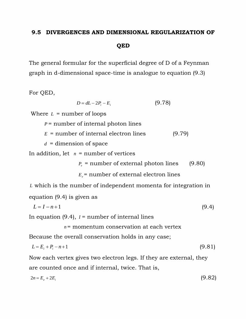
The general formular for the superficial degree of D of a Feynman

graph in d-dimensional space-time is analogue to equation (9.3)

For QED,

ii EPdLD 2 (9.78)

Where L = number of loops

P = number of internal photon lines

E = number of internal electron lines (9.79)

d = dimension of space

In addition, let n = number of vertices

eP = number of external photon lines (9.80)

eE = number of external electron lines

L which is the number of independent momenta for integration in

equation (9.4) is given as

1 nIL (9.4)

In equation (9.4), I = number of internal lines

n = momentum conservation at each vertex

Because the overall conservation holds in any case;

1 nPEL ii (9.81)

Now each vertex gives two electron legs. If they are external, they

are counted once and if internal, twice. That is,

ie EEn 22 (9.82)

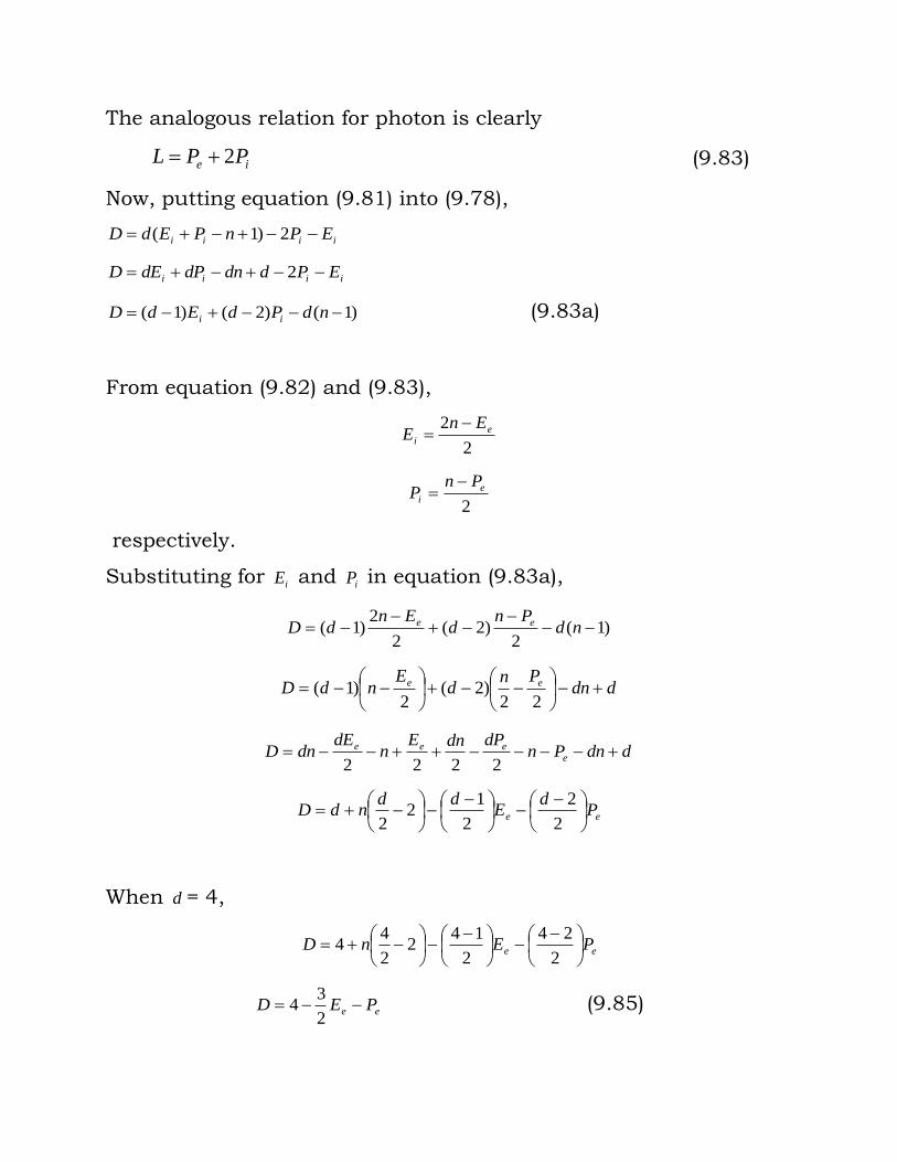
The analogous relation for photon is clearly

ie PPL 2 (9.83)

Now, putting equation (9.81) into (9.78),

iiii EPnPEdD 2)1(

iiii EPddndPdED 2

)1()2()1( ndPdEdD ii (9.83a)

From equation (9.82) and (9.83),

2

2 e

i

EnE

2

e

i

PnP

respectively.

Substituting for iE and iP in equation (9.83a),

)1(2

)2(2

2)1(

nd

Pnd

EndD ee

ddnPn

dE

ndD ee

22)2(

2)1(

ddnPndPdnE

ndE

dnD e

eee 2222

ee Pd

Edd

ndD

2

2

2

12

2

When d = 4,

ee PEnD

2

24

2

142

2

44

ee PED 2

34 (9.85)

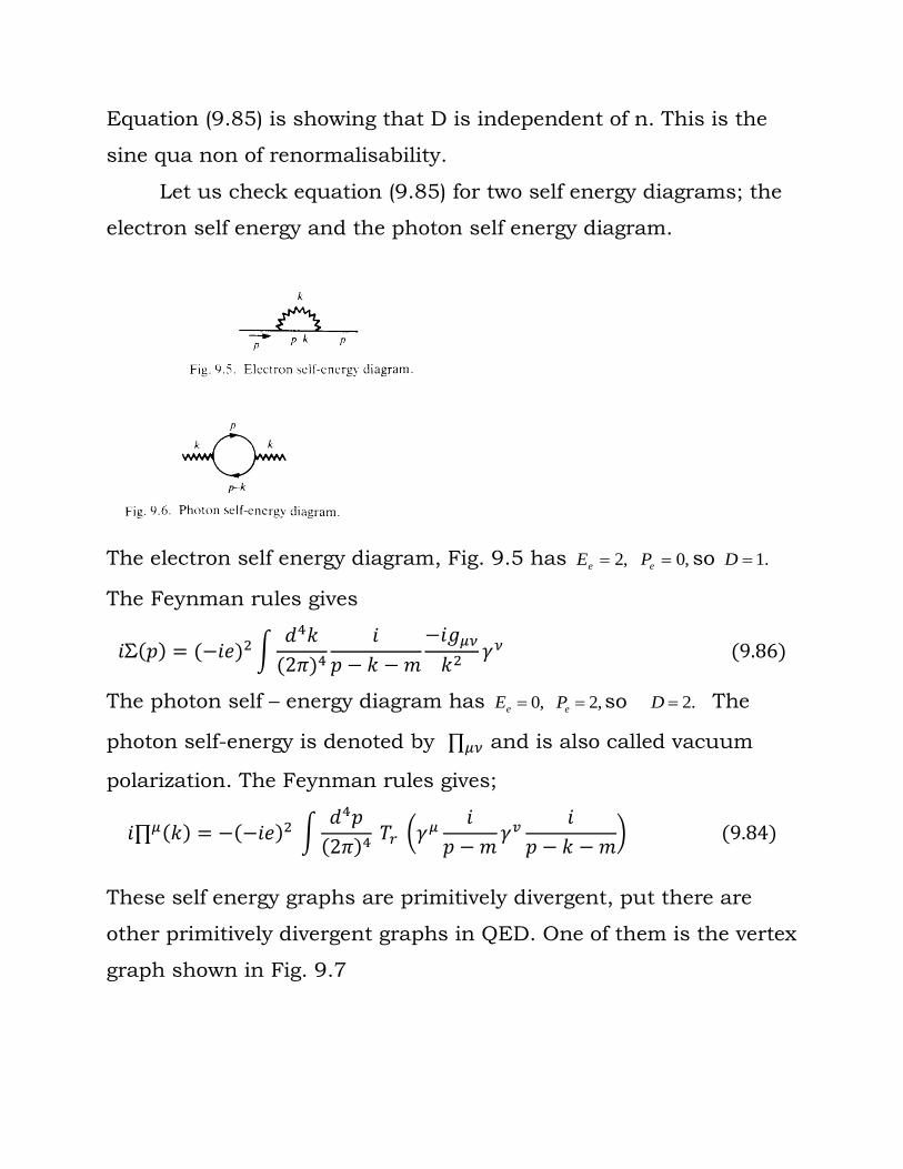
Equation (9.85) is showing that D is independent of n. This is the

sine qua non of renormalisability.

Let us check equation (9.85) for two self energy diagrams; the

electron self energy and the photon self energy diagram.

The electron self energy diagram, Fig. 9.5 has ,2eE ,0eP so .1D

The Feynman rules gives

The photon self – energy diagram has ,0eE ,2eP so .2D The

photon self-energy is denoted by and is also called vacuum

polarization. The Feynman rules gives;

These self energy graphs are primitively divergent, put there are

other primitively divergent graphs in QED. One of them is the vertex

graph shown in Fig. 9.7

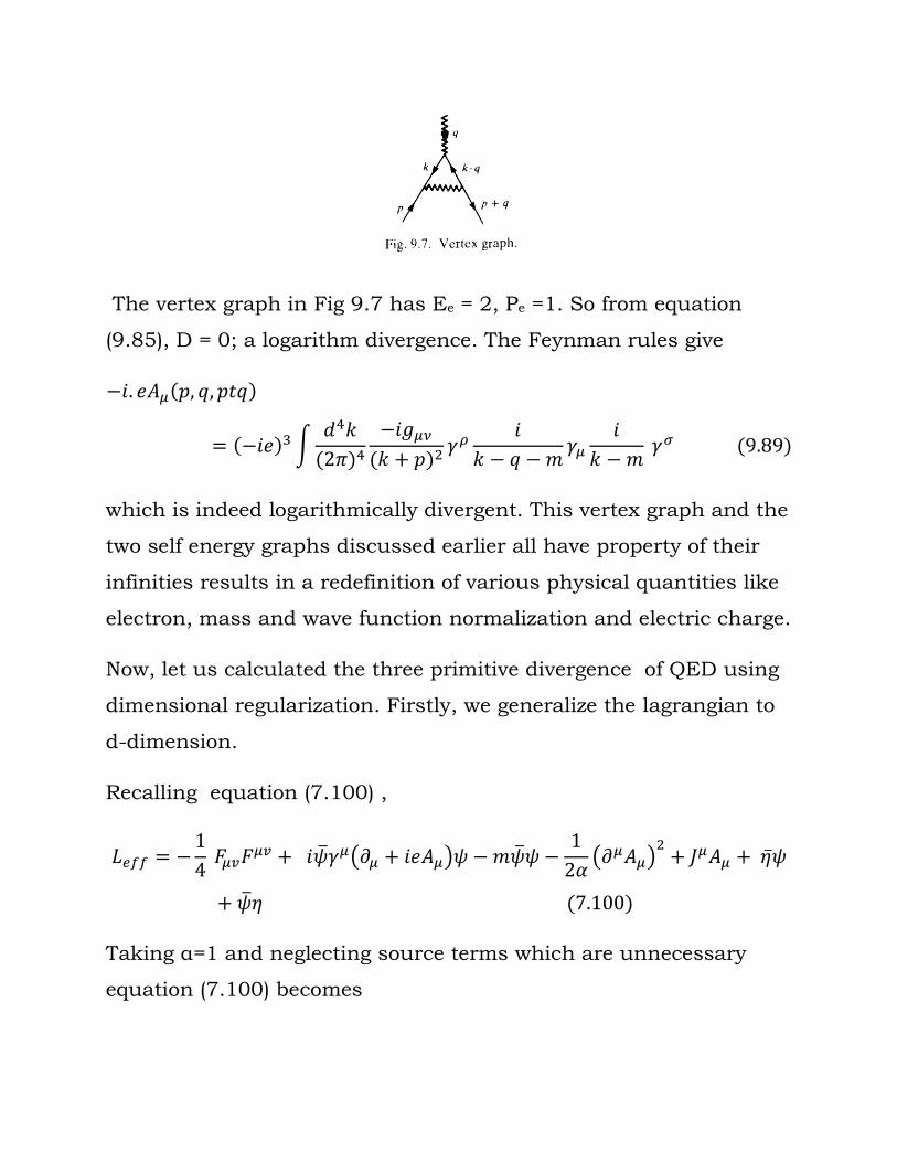
The vertex graph in Fig 9.7 has Ee = 2, Pe =1. So from equation

(9.85), D = 0; a logarithm divergence. The Feynman rules give

which is indeed logarithmically divergent. This vertex graph and the

two self energy graphs discussed earlier all have property of their

infinities results in a redefinition of various physical quantities like

electron, mass and wave function normalization and electric charge.

Now, let us calculated the three primitive divergence of QED using

dimensional regularization. Firstly, we generalize the lagrangian to

d-dimension.

Recalling equation (7.100) ,

Taking α=1 and neglecting source terms which are unnecessary

equation (7.100) becomes

All the three terms in equation (7.100a) has the right dimension

except the third. To get the third one right, must be

multiplied with e.

Here, is an arbitrary mass[5].

After the multiplication, equation (7.100a) becomes

)

Now let consider the definition and algebra of Dirac matrices in d-

dimensions. We modify the dirac matrices as follows; beginning

with the anticommutator,

Where which is the metric tensor in minkowski space is defined

in d-dimension so that,

For consistency, it then implies that

In addition, stating unmodified trace identities,

Tr (odd number of γ matrices) =0

(9.93)

Where f(d) is an arbitrary well behaved function with f(4) =4. The

analogues of cannot be given in d - dimension. So in four

dimension, we have

The levi- civita symbol specific for d=4.

Going back to the primitively divergent diagrams. Let us start with

the fermion self energy graph of fig 9.5.

The generalized expression of (9.86) to d - dimension gives

Multiplying (p-k+m) to the numerator and denominator,

Putting

Introducing the Feynman parameter Z, i.e recalling the relation

equation (9.22)

So that

Equation 9.96c becomes,

Defining gives

The linear term in Integrate to zero, so

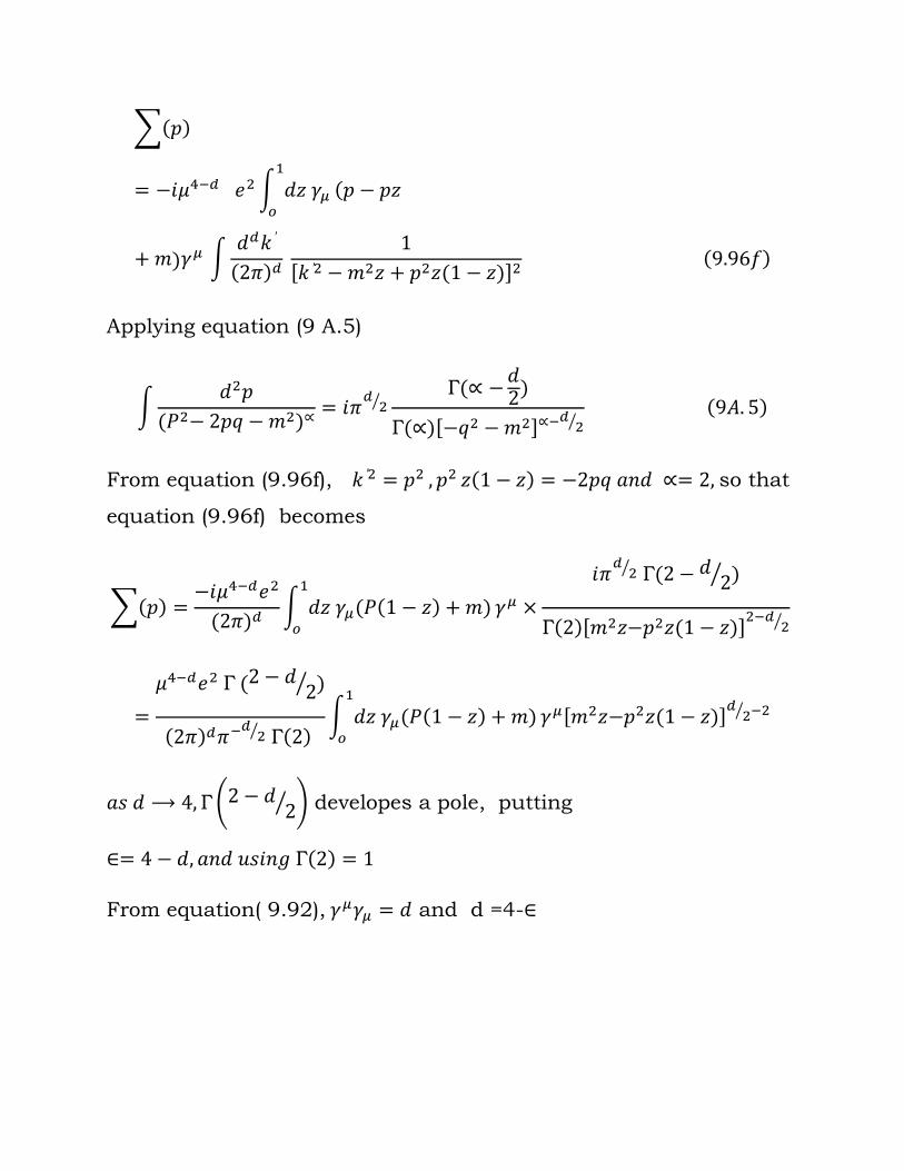
Applying equation (9 A.5)

From equation (9.96f), so that

equation (9.96f) becomes

developes a pole, putting

From equation( 9.92), and d =4-

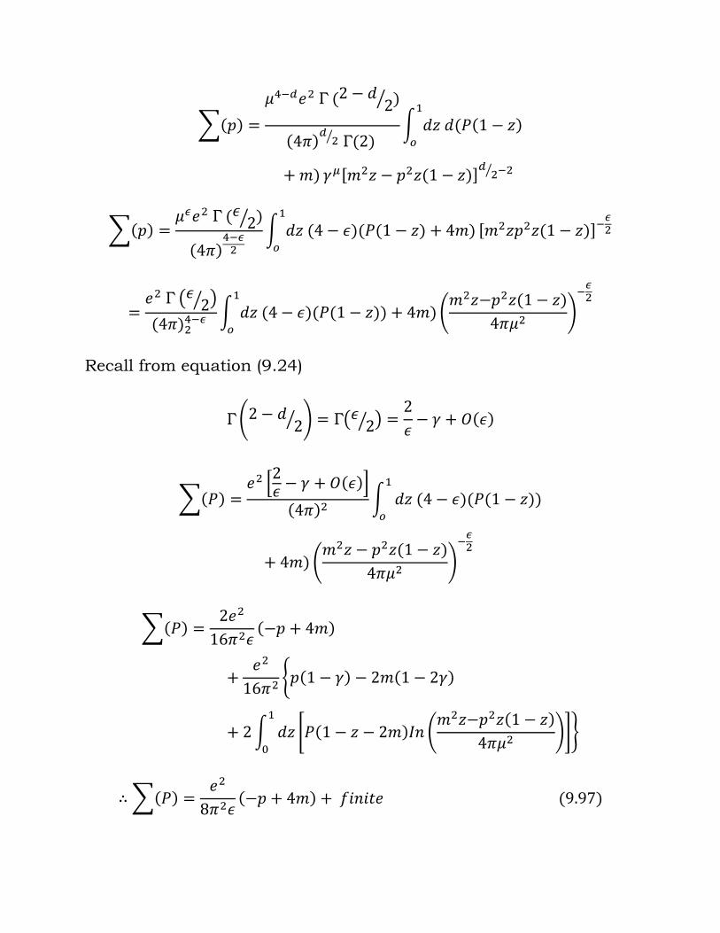
Recall from equation (9.24)

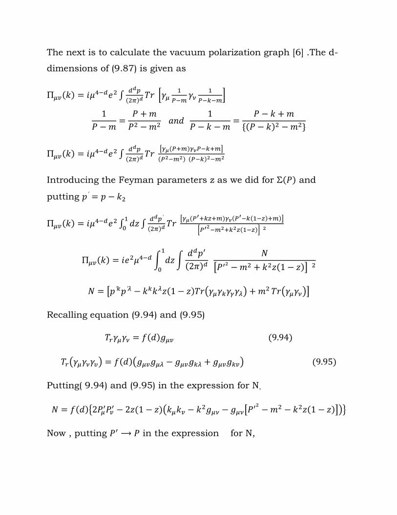
The next is to calculate the vacuum polarization graph [6] .The d-

dimensions of (9.87) is given as

Introducing the Feyman parameters z as we did for and

putting

Recalling equation (9.94) and (9.95)

Putting( 9.94) and (9.95) in the expression for N,

Now , putting in the expression for N,

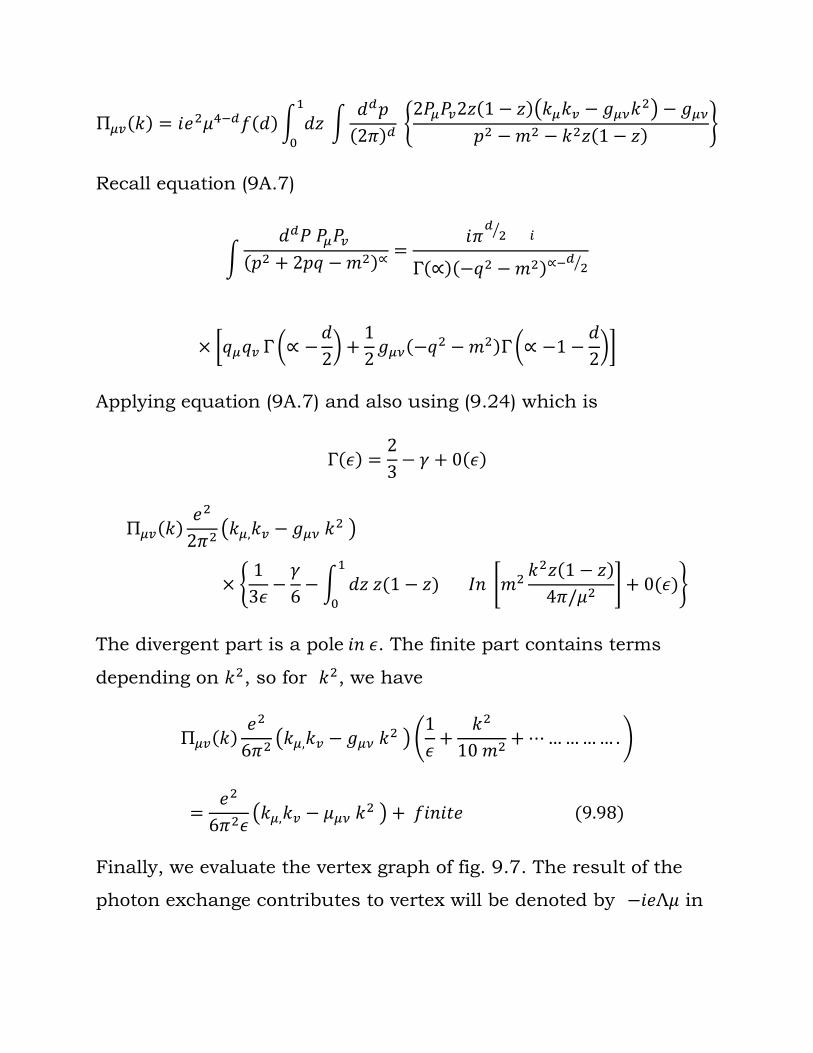
Recall equation (9A.7)

Applying equation (9A.7) and also using (9.24) which is

The divergent part is a pole . The finite part contains terms

depending on , so for , we have

Finally, we evaluate the vertex graph of fig. 9.7. The result of the

photon exchange contributes to vertex will be denoted by in

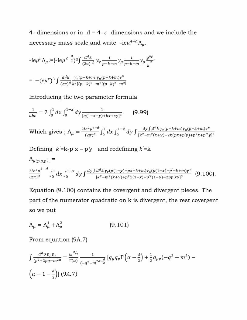
4- dimensions or in d = 4- dimensions and we include the

necessary mass scale and write -ie .

-ie .=(-ie

3

-

=

Introducing the two parameter formula

(9.99)

Which gives ;

Defining =k-p x – p y and redefining =k

(9.100).

Equation (9.100) contains the covergent and divergent pieces. The

part of the numerator quadratic on k is divergent, the rest covergent

so we put

(9.101)

From equation (9A.7)

[

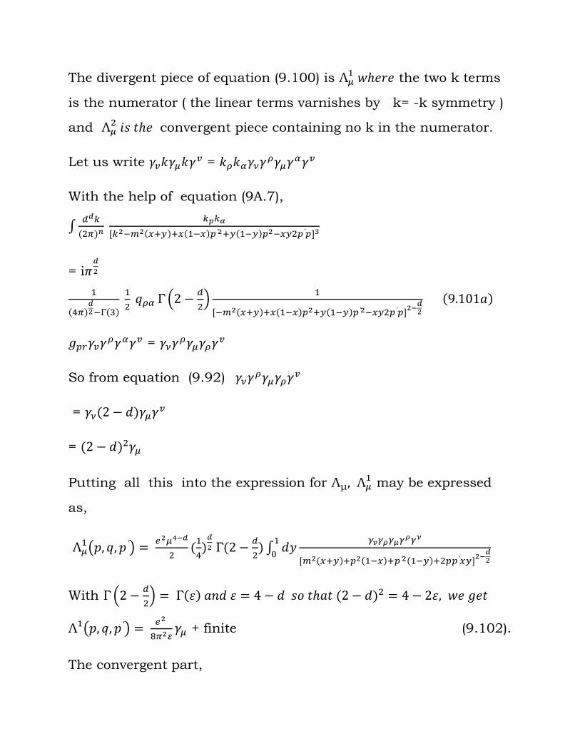
The divergent piece of equation (9.100) is the two k terms

is the numerator ( the linear terms varnishes by k= -k symmetry )

and convergent piece containing no k in the numerator.

Let us write =

With the help of equation (9A.7),

= i

=

So from equation (9.92)

=

=

Putting all this into the expression for may be expressed

as,

With

+ finite (9.102).

The convergent part,

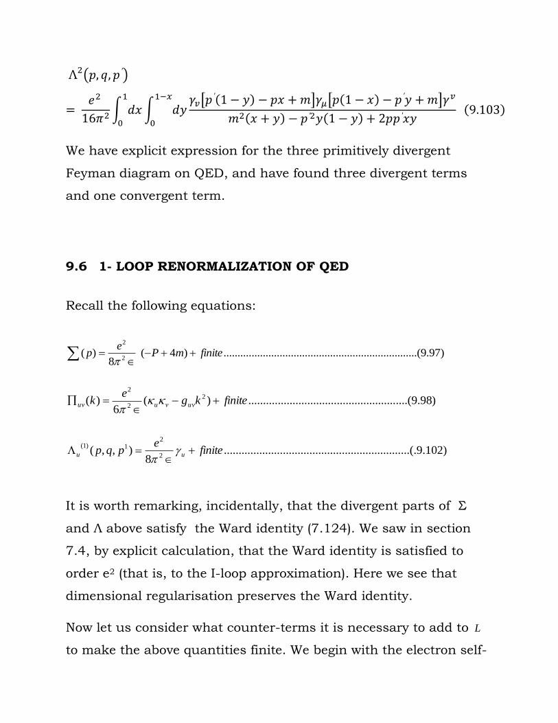
We have explicit expression for the three primitively divergent

Feyman diagram on QED, and have found three divergent terms

and one convergent term.

9.6 1- LOOP RENORMALIZATION OF QED

Recall the following equations:

)97.9.........(............................................................)4(8

)(2

2

finitemPe

p

)102.9...(.............................................................8

),,(

)98.9....(..................................................)(6

)(

2

21)1(

2

2

2

finitee

pqp

finitekge

k

uu

uvvuuv

It is worth remarking, incidentally, that the divergent parts of

and above satisfy the Ward identity (7.124). We saw in section

7.4, by explicit calculation, that the Ward identity is satisfied to

order e2 (that is, to the I-loop approximation). Here we see that

dimensional regularisation preserves the Ward identity.

Now let us consider what counter-terms it is necessary to add to L

to make the above quantities finite. We begin with the electron self-

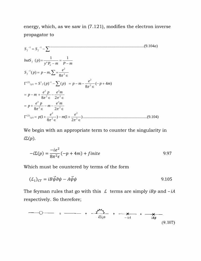
energy, which, as we saw in (7.121), modifies the electron inverse

propagator to

)104.9.....(............................................................)2

1()8

1(

28

28

)4(8

)()(

8,)(

11)(

)104.9.....(..........................................................................................

2

2

2

2

)()2(

2

2

2

2

2

2

2

2

2

211

)()2(

2

21

11

em

ep

mem

pep

mepemp

mpe

mpppS

emppS

mPmPypbutS

aSS

p

fp

f

u

uf

ff

We begin with an appropriate term to counter the singularity in

Which must be countered by terms of the form

The feyman rules that go with this terms are simply and –

respectively. So therefore;

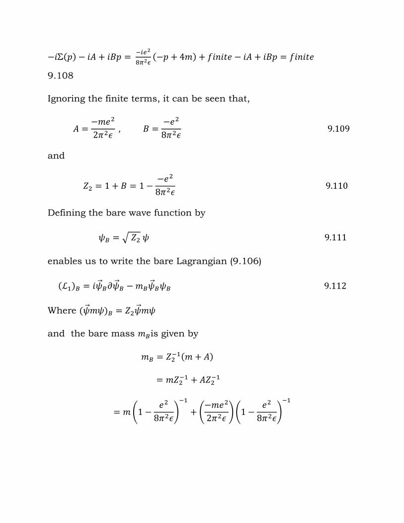
9.108

Ignoring the finite terms, it can be seen that,

and

Defining the bare wave function by

enables us to write the bare Lagrangian (9.106)

Where

and the bare mass is given by

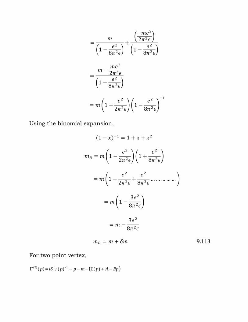
Using the binomial expansion,

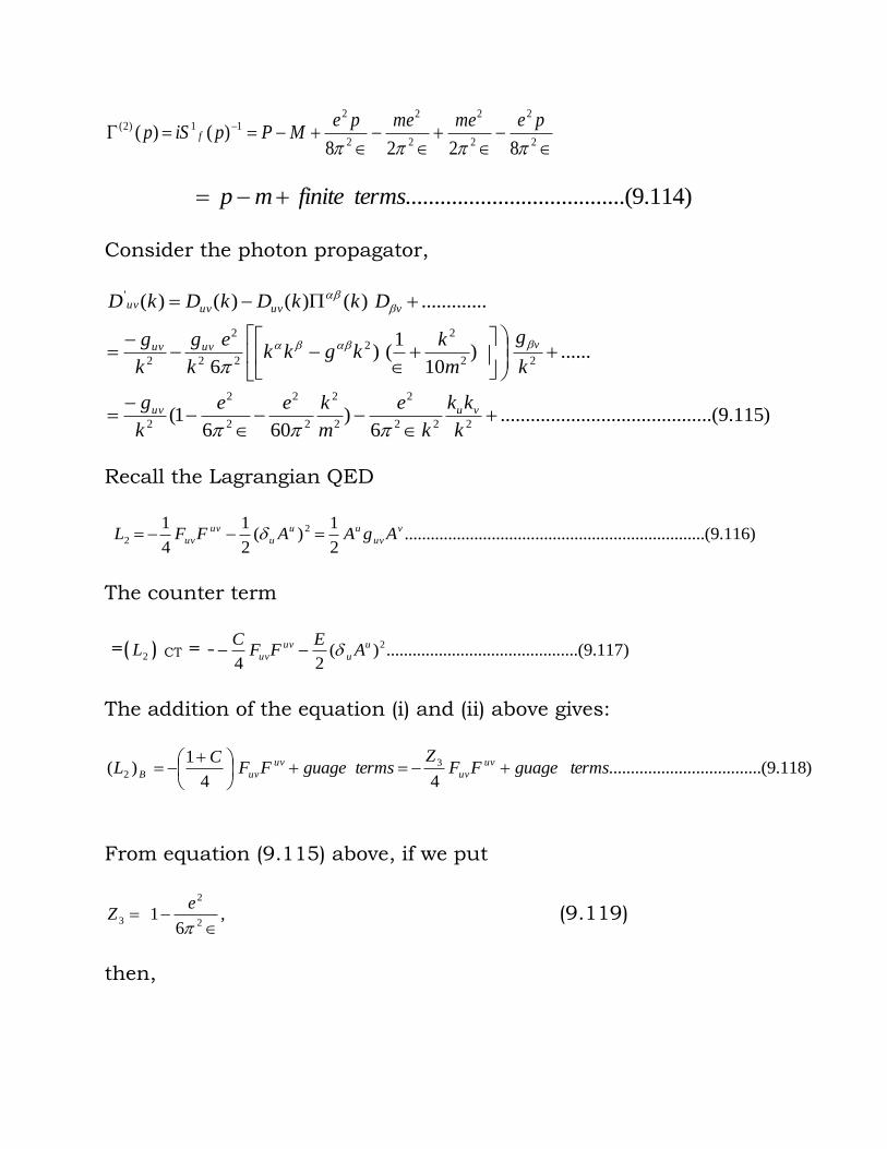
For two point vertex,

BpApmppiSp f )()()( 11)2(

2

2

2

2

2

2

2

211)2(

8228)()(

pememepeMPpiSp f

)114.9........(..............................termsfinitemp

Consider the photon propagator,

)115.9..(........................................6

)606

1(

......)10

1()

6

.............)()()()(

222

2

2

2

2

2

2

2

2

22

22

22

2

2

'

k

kk

k

e

m

kee

k

g

k

g

m

kkgkk

k

eg

k

g

DkkDkDkD

vuuv

vuvuv

vuvuvuv

Recall the Lagrangian QED

)116.9.........(............................................................2

1)(

2

1

4

1 2

2

v

uv

uu

u

uv

uv AgAAFFL

The counter term

=( 2L ) CT = - )117.9....(........................................)(24

2u

u

uv

uv AE

FFC

The addition of the equation (i) and (ii) above gives:

)118.9.....(..............................44

1)( 3

2 termsguageFFZ

termsguageFFC

L uv

uv

uv

uvB

From equation (9.115) above, if we put

,6

12

2

3

eZ (9.119)

then,

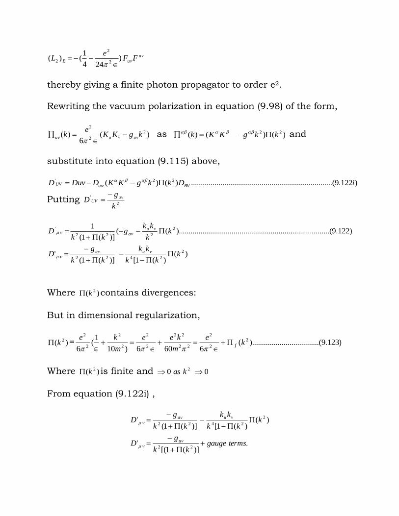
uv

uvB FFe

L )244

1()(

2

2

2

thereby giving a finite photon propagator to order e2.

Rewriting the vacuum polarization in equation (9.98) of the form,

)(6

)( 2

2

2

kgKKe

k uvvuuv

as )()()( 22 kkgKKk and

substitute into equation (9.115) above,

)122.9..(......................................................................)()( 22' iDkkgKKDDuvD BVuUV

Putting 2

'

k

gD uv

UV

)()(1[)](1(

'

)122.9........(............................................................).........(()](1(

1

2

2422

2

222

'

kkk

kk

kk

gD

kk

kkg

kkD

vuav

vu

v

Where )( 2k contains divergences:

But in dimensional regularization,

)( 2k = )123.9.....(....................).........(6606)10

1(

6

2

2

2

22

22

2

2

2

2

2

2

ke

m

kee

m

kef

Where )( 2k is finite and 00 2 kas

From equation (9.122i) ,

.)](1[(

'

)()(1[)](1(

'

22

2

2422

termsgaugekk

gD

kkk

kk

kk

gD

uv

vuav

= termsguage

ke

k

g

f

uv

)(6

1[ 2

2

22

But Z3 = ,6

12

2

ethen

2

2

61

e

termsgaugekk

gZD uv

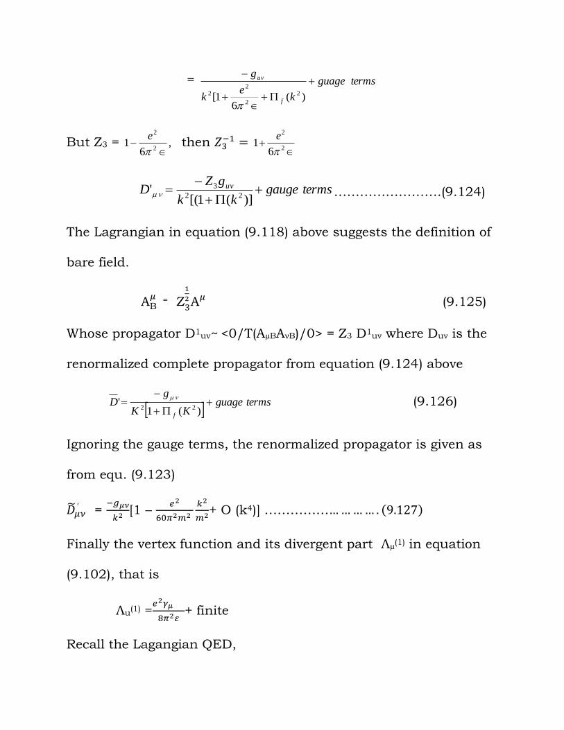
)](1[('

22

3 …………………….(9.124)

The Lagrangian in equation (9.118) above suggests the definition of

bare field.

=

(9.125)

Whose propagator D1uv~ <0/T(AµBAνB)/0> = Z3 D1

uv where Duv is the

renormalized complete propagator from equation (9.124) above

termsguage

KK

gD

f

)(1'

22

(9.126)

Ignoring the gauge terms, the renormalized propagator is given as

from equ. (9.123)

=

[1 –

+ O (k4)] ……………

Finally the vertex function and its divergent part Лµ(1) in equation

(9.102), that is

u(1) =

+ finite

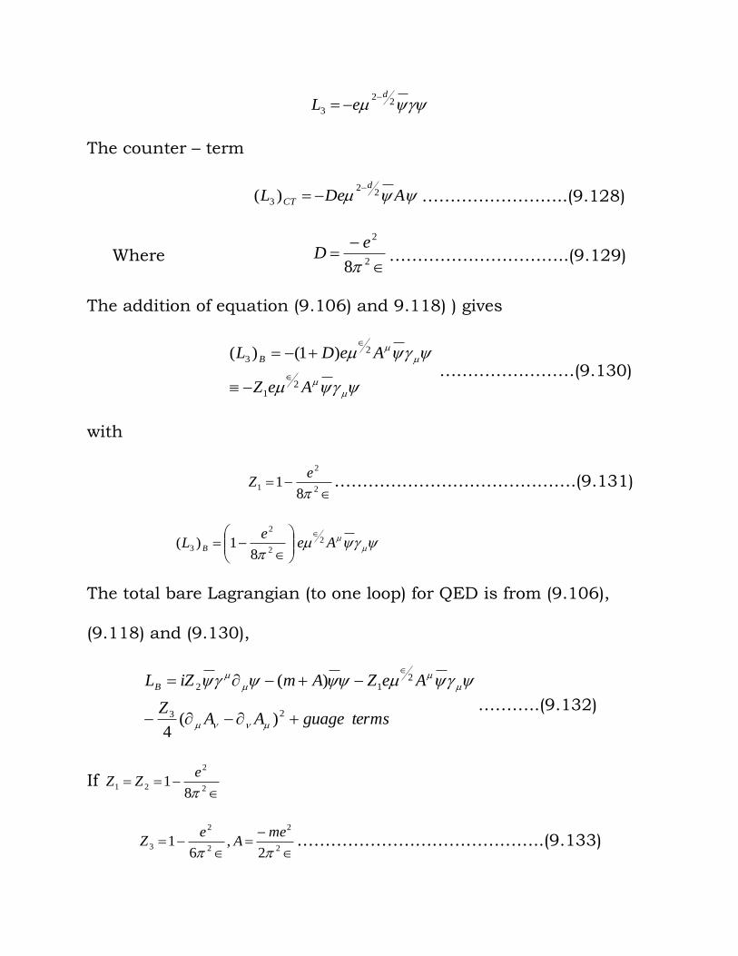
Recall the Lagangian QED,

22

3

d

eL

The counter – term

ADeLd

CT2

2

3 )(

……………………..(9.128)

Where

2

2

8

eD …………………………..(9.129)

The addition of equation (9.106) and 9.118) ) gives

AeZ

AeDL B

21

23 )1()(

……………………(9.130)

with

2

2

18

1

eZ …………………………………….(9.131)

2

2

38

1)(

eL B

Ae 2

The total bare Lagrangian (to one loop) for QED is from (9.106),

(9.118) and (9.130),

termsguageAAZ

AeZAmiZLB

23

212

)(4

)(

………..(9.132)

If

2

2

218

1

eZZ

2

2

2

2

32

,6

1

meA

eZ ……………………………………..(9.133)

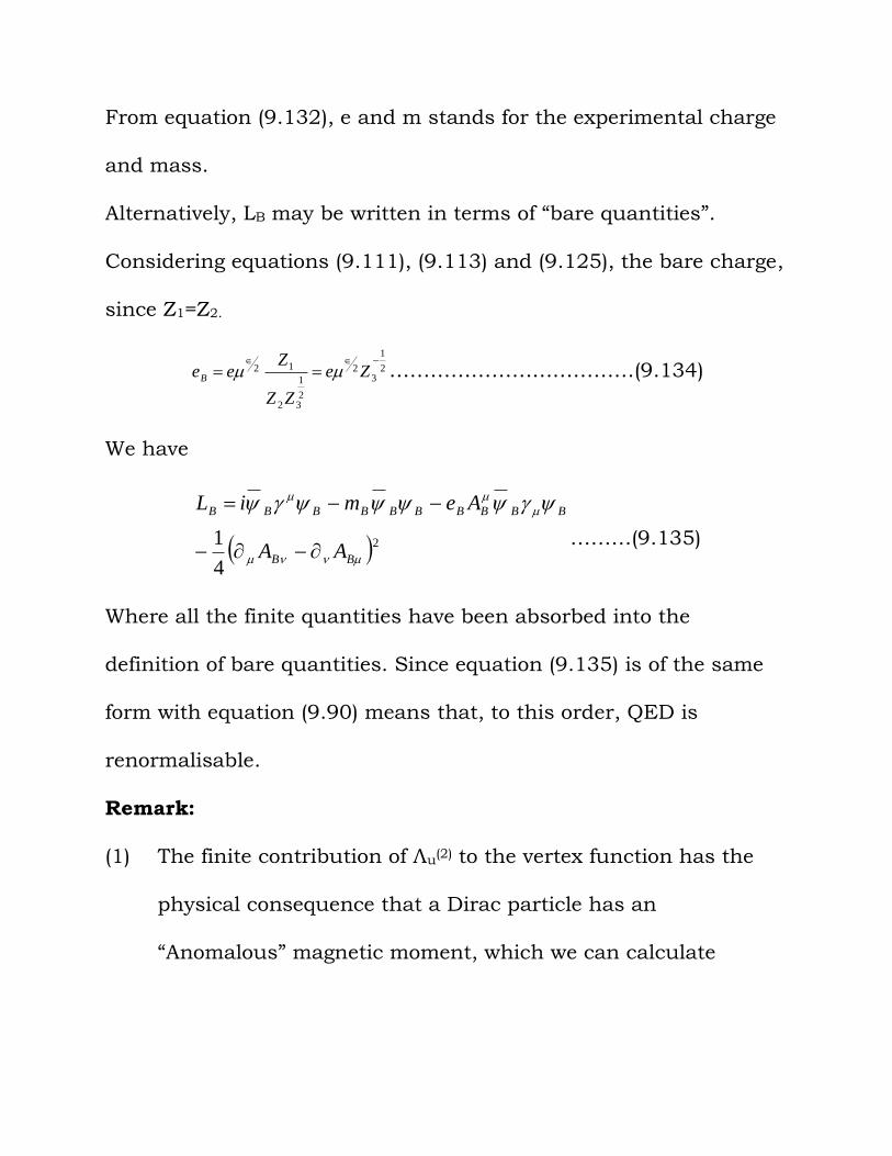
From equation (9.132), e and m stands for the experimental charge

and mass.

Alternatively, LB may be written in terms of “bare quantities”.

Considering equations (9.111), (9.113) and (9.125), the bare charge,

since Z1=Z2.

2

1

32

2

1

32

12

Ze

ZZ

ZeeB ………………………………(9.134)

We have

24

1

BB

BBBBBBBBBB

AA

AemiL

………(9.135)

Where all the finite quantities have been absorbed into the

definition of bare quantities. Since equation (9.135) is of the same

form with equation (9.90) means that, to this order, QED is

renormalisable.

Remark:

(1) The finite contribution of u(2) to the vertex function has the

physical consequence that a Dirac particle has an

“Anomalous” magnetic moment, which we can calculate

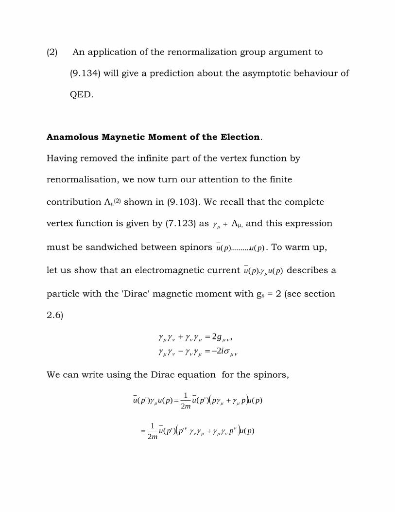
(2) An application of the renormalization group argument to

(9.134) will give a prediction about the asymptotic behaviour of

QED.

Anamolous Maynetic Moment of the Election.

Having removed the infinite part of the vertex function by

renormalisation, we now turn our attention to the finite

contribution Лµ(2) shown in (9.103). We recall that the complete

vertex function is given by (7.123) as Лµ, and this expression

must be sandwiched between spinors )(.).........( pupu . To warm up,

let us show that an electromagnetic current )().( pupu describes a

particle with the 'Dirac' magnetic moment with gs = 2 (see section

2.6)

i

g

2

,2

We can write using the Dirac equation for the spinors,

)()'(2

1)()'( pupppu

mpupu

)(')'(2

1pupppu

m

)(')'(2

1pupigigppu

m

)(')'(2

1puqipppu

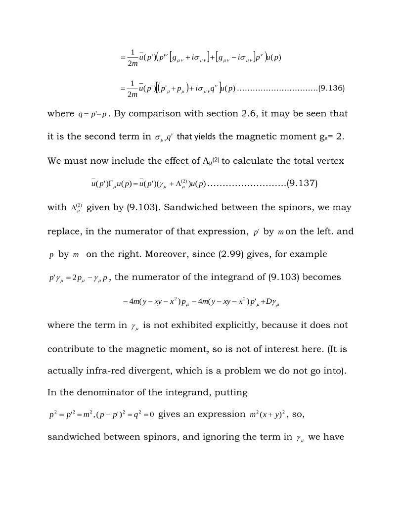
m

………………………….(9.136)

where ppq ' . By comparison with section 2.6, it may be seen that

it is the second term in q that yields the magnetic moment gs= 2.

We must now include the effect of µ(2) to calculate the total vertex

)())('()()'( )2( pupupupu ……………………..(9.137)

with )2(

given by (9.103). Sandwiched between the spinors, we may

replace, in the numerator of that expression, 'p by m on the left. and

p by m on the right. Moreover, since (2.99) gives, for example

ppp 2' , the numerator of the integrand of (9.103) becomes

Dpxxyympxxyym ')(4)(4 22

where the term in is not exhibited explicitly, because it does not

contribute to the magnetic moment, so is not of interest here. (It is

actually infra-red divergent, which is a problem we do not go into).

In the denominator of the integrand, putting

0)'(,' 22222 qppmpp gives an expression 22 )( yxm , so,

sandwiched between spinors, and ignoring the term in we have

')()()(

1

4

221

0 2

1

02

2)2( pyxyxpxxyy

yxdydx

m

e x

)'(16 2

2

ppm

e

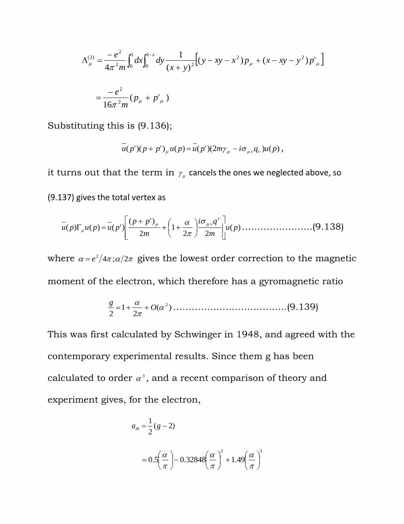
Substituting this is (9.136);

)()2)('()()')('( puqimpupupppu ,

it turns out that the term in cancels the ones we neglected above, so

(9.137) gives the total vertex as

)(22

12

)'()'()()( pu

m

qi

m

pppupupu

…………………..(9.138)

where 2;42e gives the lowest order correction to the magnetic

moment of the electron, which therefore has a gyromagnetic ratio

)(2

12

2

O

g ……………………………….(9.139)

This was first calculated by Schwinger in 1948, and agreed with the

contemporary experimental results. Since them g has been

calculated to order 3 , and a recent comparison of theory and

experiment gives, for the electron,

)2(2

1 gath

32

49.132848.05.0

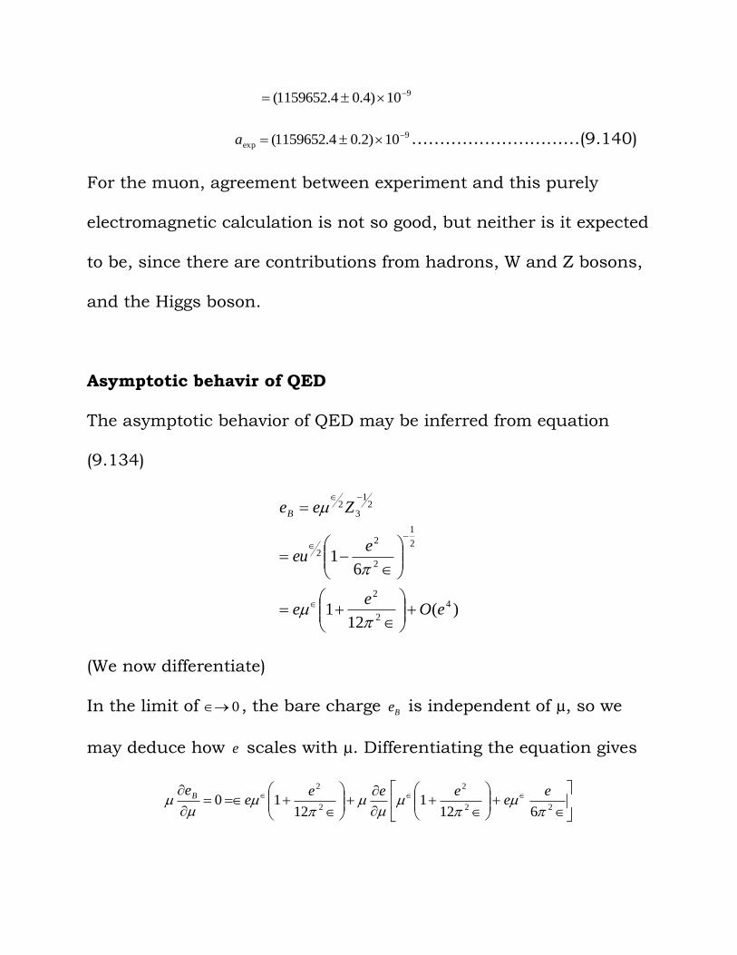
910)4.04.1159652(

9

exp 10)2.04.1159652( a …………………………(9.140)

For the muon, agreement between experiment and this purely

electromagnetic calculation is not so good, but neither is it expected

to be, since there are contributions from hadrons, W and Z bosons,

and the Higgs boson.

Asymptotic behavir of QED

The asymptotic behavior of QED may be inferred from equation

(9.134)

)(12

1

61

4

2

2

2

1

2

2

2

21

32

eOe

e

eeu

ZeeB

(We now differentiate)

In the limit of 0 , the bare charge Be is independent of µ, so we

may deduce how e scales with µ. Differentiating the equation gives

22

2

2

2

6121

1210

ee

eeee

eB

2

2

2

2

81

1210

eeee

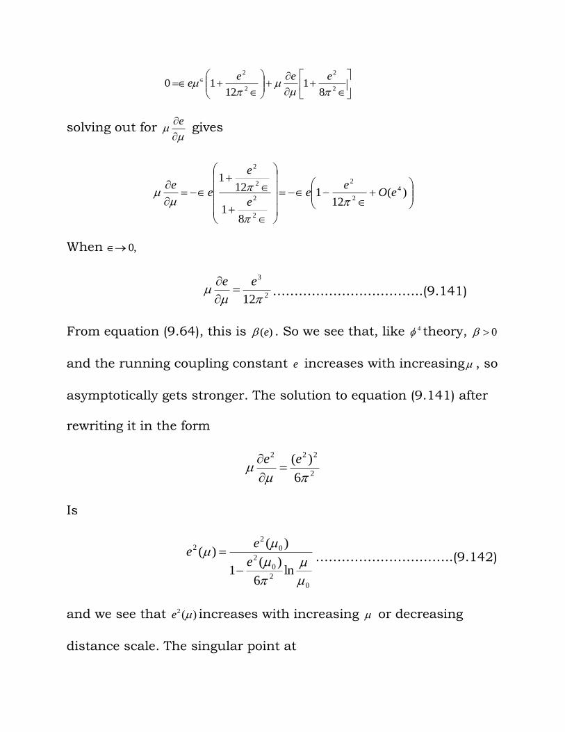
solving out for

e gives

)(

121

81

121

4

2

2

2

2

2

2

eOe

ee

e

ee

When ,0

2

3

12

ee

……………………………..(9.141)

From equation (9.64), this is )(e . So we see that, like 4 theory, 0

and the running coupling constant e increases with increasing , so

asymptotically gets stronger. The solution to equation (9.141) after

rewriting it in the form

2

222

6

)(

ee

Is

0

2

0

2

0

22

ln6

)(1

)()(

e

ee

…………………………..(9.142)

and we see that )(2 e increases with increasing or decreasing

distance scale. The singular point at

)(

6exp

0

2

2

0

e

is referred to as Landau singularity.

9.8 ASYMPTOTIC FREEDOM OF YANG-MILLS THEORIES

Asymptotic freedom is the flow of coupling constant to an

ultraviolet fixed point where it vanishes. In asymptotically free

theories, the interacting particles are essentially free at short

distances and high energies. We shall perform calculations in order

to show that at high energies the running coupling in yang-mills

theories approaches zero. The asymptotic freedom is a property

possessed by all non-Abelian gauge theories, and, so far is known,

only by non-Abelian gauge theories [1]. In quantum

electrodynamics (QED), the coupling constant increases with energy

due to screening. It is known that quarks act as free particles at

high energies. The general case shall not be studied, but we confine

ourselves for definiteness and because of the physical relevance of

QCD, to SU(3) gauge symmetry[7].

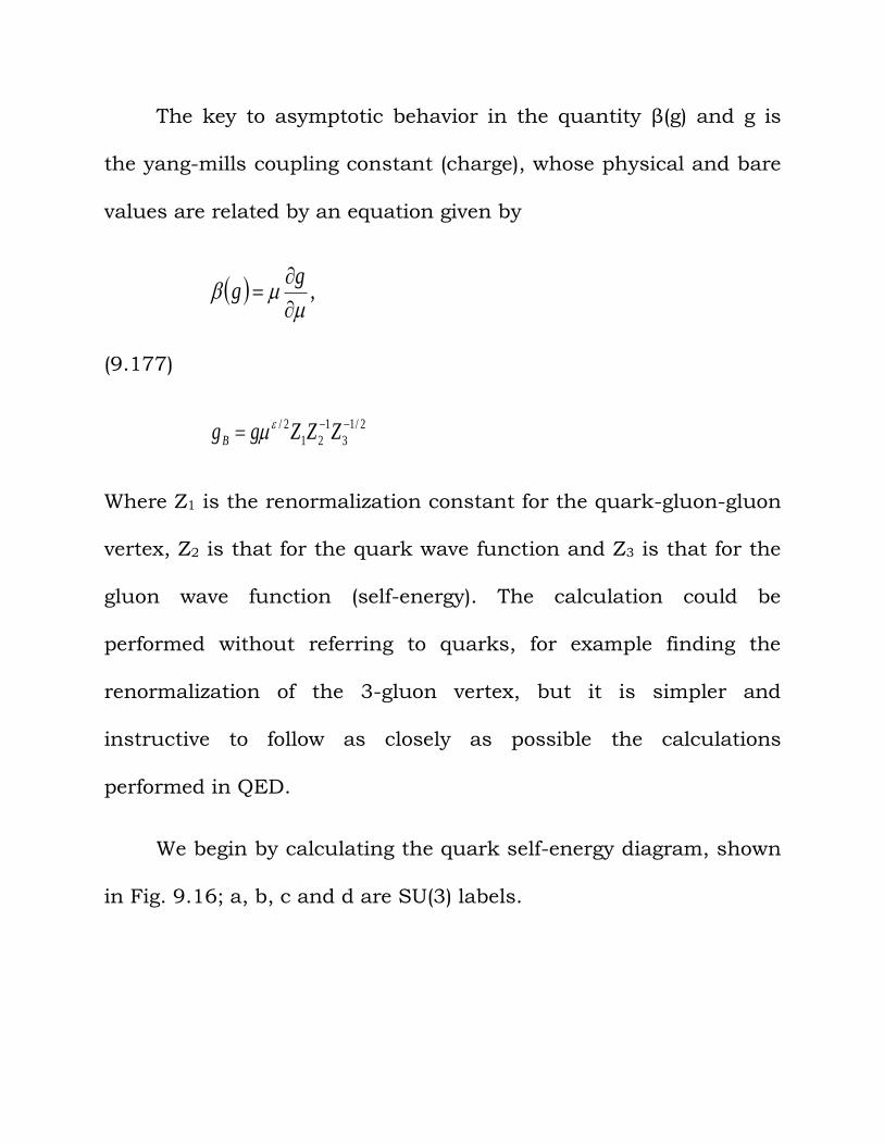
The key to asymptotic behavior in the quantity β(g) and g is

the yang-mills coupling constant (charge), whose physical and bare

values are related by an equation given by

,

gg

(9.177)

2/1

3

1

21

2/ ZZZggB

Where Z1 is the renormalization constant for the quark-gluon-gluon

vertex, Z2 is that for the quark wave function and Z3 is that for the

gluon wave function (self-energy). The calculation could be

performed without referring to quarks, for example finding the

renormalization of the 3-gluon vertex, but it is simpler and

instructive to follow as closely as possible the calculations

performed in QED.

We begin by calculating the quark self-energy diagram, shown

in Fig. 9.16; a, b, c and d are SU(3) labels.

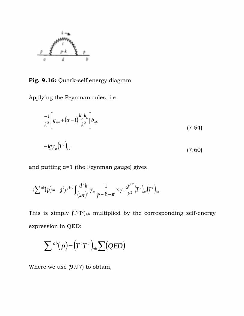
Fig. 9.16: Quark-self energy diagram

Applying the Feynman rules, i.e

abk

kkg

k

i

22

1

(7.54)

ab

cTig (7.60)

and putting α=1 (the Feynman gauge) gives

db

c

ad

c

d

ddab TT

k

g

mkp

kdgpi

2

42 1

2

This is simply (TcTc)ab multiplied by the corresponding self-energy

expression in QED:

QEDTTp ab

ccab

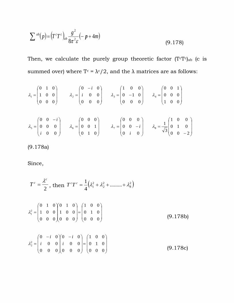
Where we use (9.97) to obtain,

mpg

TTp ab

ccab 48 2

2

(9.178)

Then, we calculate the purely group theoretic factor (TcTc)ab (c is

summed over) where Tc = λc/2, and the λ matrices are as follows:

000

001

010

1

000

00

00

2 i

i

000

010

001

3

001

000

100

4

00

000

00

5

i

i

010

100

000

6

00

00

000

7

i

i

200

010

001

3

18

(9.178a)

Since,

2

ccT

, then 2

8

2

2

2

1 .........4

1 ccTT

000

010

001

000

001

010

000

001

0102

1

(9.178b)

000

010

001

000

00

00

000

00

002

2 i

i

i

i

(9.178c)

000

010

001

000

010

001

000

010

0012

3

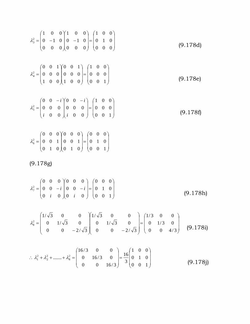
(9.178d)

100

000

001

001

000

100

001

000

1002

4

(9.178e)

100

000

001

00

000

00

00

000

002

5

i

i

i

i

(9.178f)

100

010

000

010

100

000

010

100

0002

6

(9.178g)

100

010

000

00

00

000

00

00

0002

7

i

i

i

i

(9.178h)

3/400

03/10

003/1

3/200

03/10

003/1

3/200

03/10

003/12

8

(9.178i)

100

010

001

3

16

3/1600

03/160

003/16

....... 2

8

2

2

2

1 (9.178j)

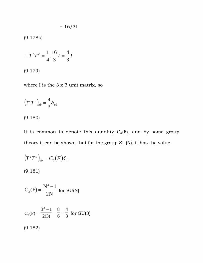
= 16/3I

(9.178k)

IITT cc

3

4

3

16.

4

1

(9.179)

where I is the 3 x 3 unit matrix, so

abab

ccTT 3

4

(9.180)

It is common to denote this quantity C2(F), and by some group

theory it can be shown that for the group SU(N), it has the value

abab

cc FCTT 2

(9.181)

N2

1N)F(C

2

2

for SU(N)

)F(C2 3

4

6

8

)3(2

132

for SU(3)

(9.182)

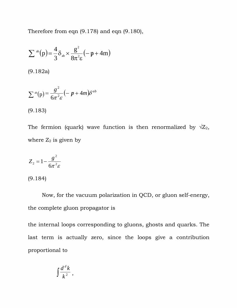
Therefore from eqn (9.178) and eqn (9.180),

m4p8

g

3

4p

2

2

ab

ab

(9.182a)

pab

abmpg

46 2

2

(9.183)

The fermion (quark) wave function is then renormalized by √Z2,

where Z2 is given by

2

2

26

1g

Z

(9.184)

Now, for the vacuum polarization in QCD, or gluon self-energy,

the complete gluon propagator is

the internal loops corresponding to gluons, ghosts and quarks. The

last term is actually zero, since the loops give a contribution

proportional to

2k

kd d

,

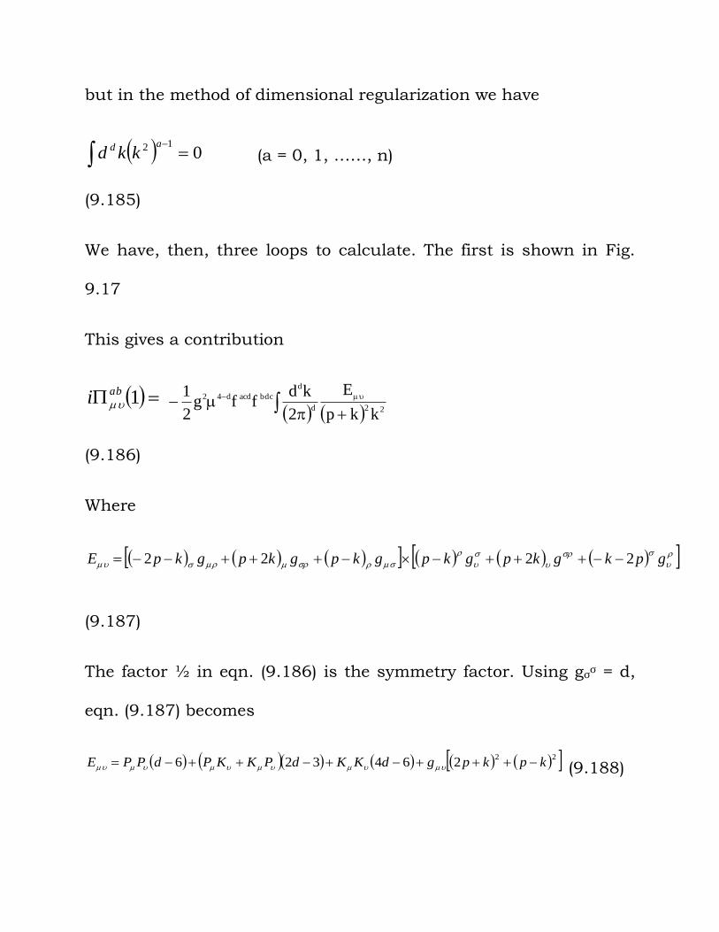
but in the method of dimensional regularization we have

012 ad kkd (a = 0, 1, ……, n)

(9.185)

We have, then, three loops to calculate. The first is shown in Fig.

9.17

This gives a contribution

1abi

22d

d

bdcacdd42

kkp

E

2

kdffg

2

1

(9.186)

Where

gpkgkpgkpgkpgkpgkpE 2222

(9.187)

The factor ½ in eqn. (9.186) is the symmetry factor. Using gσσ = d,

eqn. (9.187) becomes

22264326 kpkpgdKKdPKKPdPPE (9.188)

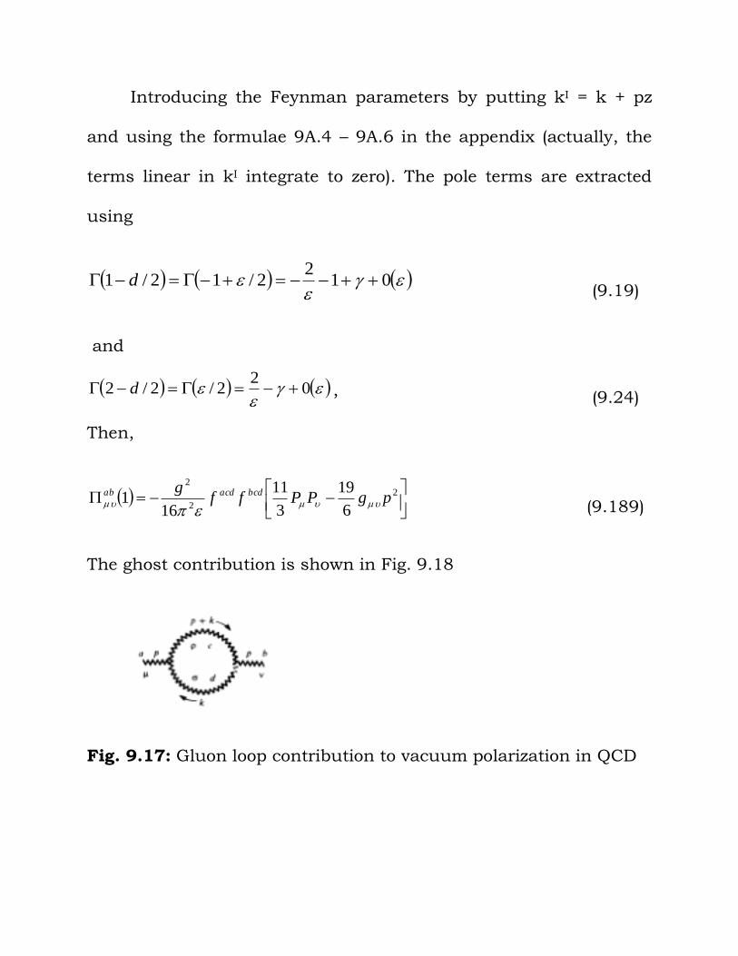
Introducing the Feynman parameters by putting kI = k + pz

and using the formulae 9A.4 – 9A.6 in the appendix (actually, the

terms linear in kI integrate to zero). The pole terms are extracted

using

012

2/12/1 d (9.19)

and

02

2/2/2 d , (9.24)

Then,

2

2

2

6

19

3

11

161 pgPPff

g bcdacdab

(9.189)

The ghost contribution is shown in Fig. 9.18

Fig. 9.17: Gluon loop contribution to vacuum polarization in QCD

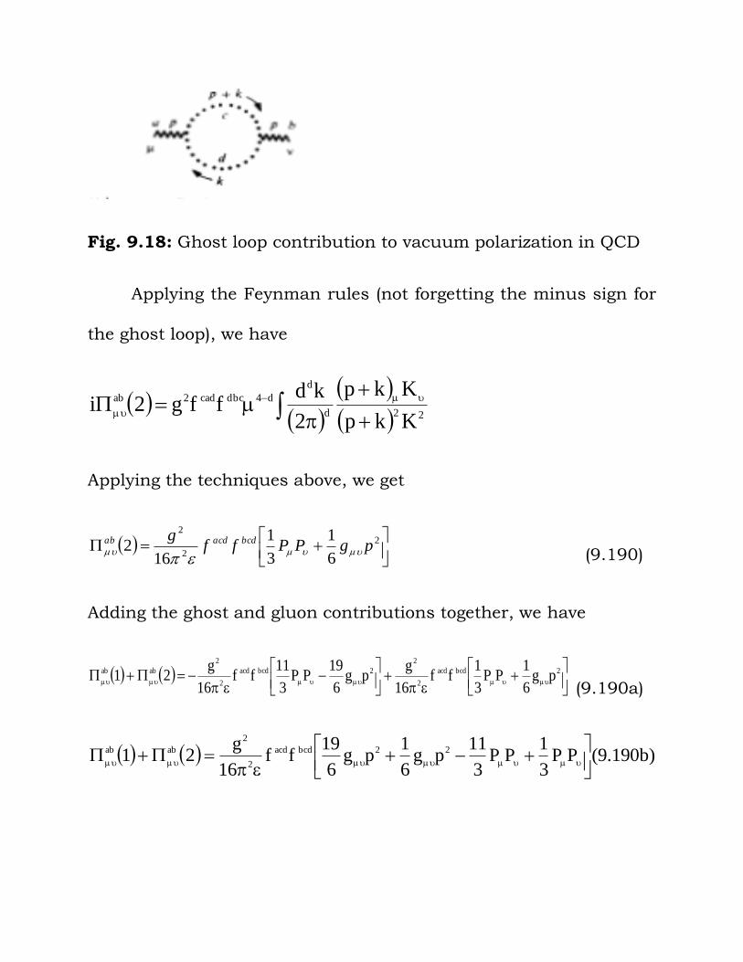
Fig. 9.18: Ghost loop contribution to vacuum polarization in QCD

Applying the Feynman rules (not forgetting the minus sign for

the ghost loop), we have

22d

d

d4dbccad2ab

Kkp

Kkp

2

kdffg2i

Applying the techniques above, we get

2

2

2

6

1

3

1

162 pgPPff

g bcdacdab

(9.190)

Adding the ghost and gluon contributions together, we have

2bcdacd

2

2

2bcdacd

2

2

abab pg6

1PP

3

1ff

16

gpg

6

19PP

3

11ff

16

g21

(9.190a)

)b190.9(PP3

1PP

3

11pg

6

1pg

6

19ff

16

g21 22bcdacd

2

2

abab

PP

3

10pg

3

10ff

16

g21 2bcdacd

2

2

abab

(9.190c)

PPpg3

10.ff

16

g21 2bcdacd

2

2

abab

(9.190d)

PPpgffg bcdacdab 2

2

2

3

5.

821

(9.191)

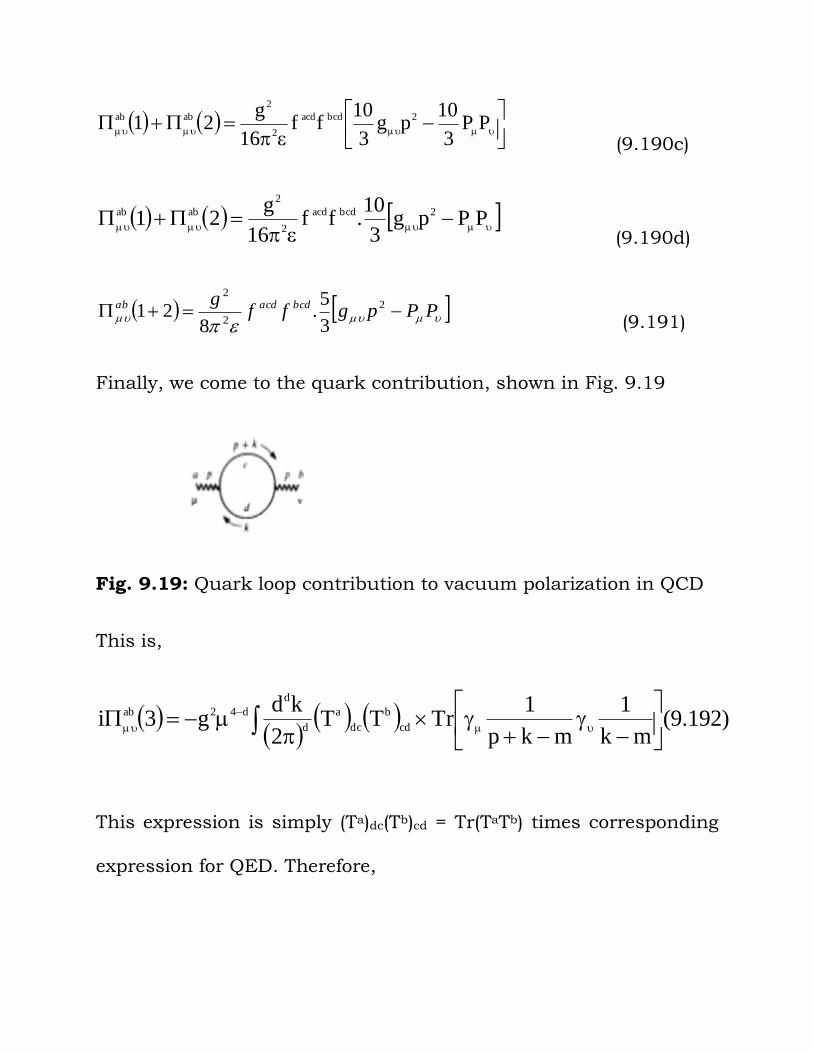
Finally, we come to the quark contribution, shown in Fig. 9.19

Fig. 9.19: Quark loop contribution to vacuum polarization in QCD

This is,

)192.9(mk

1

mkp

1TrTT

2

kdg3i cd

b

dc

a

d

d

d42ab

This expression is simply (Ta)dc(Tb)cd = Tr(TaTb) times corresponding

expression for QED. Therefore,

2

2

2

63 pgPP

gTTTr baab

(9.193)

We now calculate the group theoretic factors appearing in equations

(9.191) and (9.193). The λ matrices are normalized such that

Trλaλb = 2δab

But Ta = λa/2 and Tb = λb/2

Therefore, λaλb = 4TaTb

4Tr(TaTb) = 2δab

Tr(TaTb) = 2δab/4 = ½ δab

This is what would be substituted in eqn. (9.193) if only quarks

belonging to one representation of SU(3) contributed to the vacuum

polarization; or, in other words, if there were only one ‘flavour’ of

quark carrying the SU(3) colour label. But we know this is not true

because there are at least six flavours of quarks and possibly more.

So if nF is the number of quark flavours, we have:

Tr(TaTb) = nF/2 δab

(9.194)

But facdfbcd = 3δab

(9.195)

This number 3 is a casimir operator of the group, commonly

denoted C2(G), and the above equation is more generally written as:

facdfbcd = δabC2(G), (9.196)

C2(G) = N for SU(N)

C2(G) = 3 for SU(3) (9.197)

Gathering our results together, the vacuum polarization tensor

becomes

)a197.9(pgPP6

gTTTrPPpg

3

5ff

8

g321 2

2

2

ba2bcdacd

2

2

ab

ab2F

2

2

ab2

22

2

ab pgPP2

n

6

gPPpg

3

5GC

8

g321

(9.197b)

abF

2

2

2

2

ab

2

n

6

8GC

3

5PPpg

8

g321

(9.197c)

abF

2

2

2

2

ab

3

n2GC

3

5PPpg

8

g321

(9.197d)

But C2(G) = 3, therefore

abFab nPPpg

g

3

25

8321 2

2

2

(9.198)

The renormalization constant Z3 required to cancel this divergence

in a counter-term follows immediately by comparing the equations:

2

2

2

6pgKK

gk

, (9.98)

2

2

36

1g

Z (9.119)

Therefore,

3

25

81

2

2

3Fng

Z

(9.199)

An interesting feature of eqns (9.198) and (9.199) is that the

contributions of the ‘pure yang-mills’ terms (gluons and ghosts) and

of the quarks, to , are opposite in sign. We shall see that a

consequence of this is that asymptotic freedom depends on the

number of quark flavours.

We now calculate the quark-gluon vertex function. Two

distinct Feynman diagrams contribute to this, and are shown in

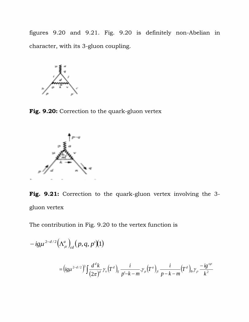
figures 9.20 and 9.21. Fig. 9.20 is definitely non-Abelian in

character, with its 3-gluon coupling.

Fig. 9.20: Correction to the quark-gluon vertex

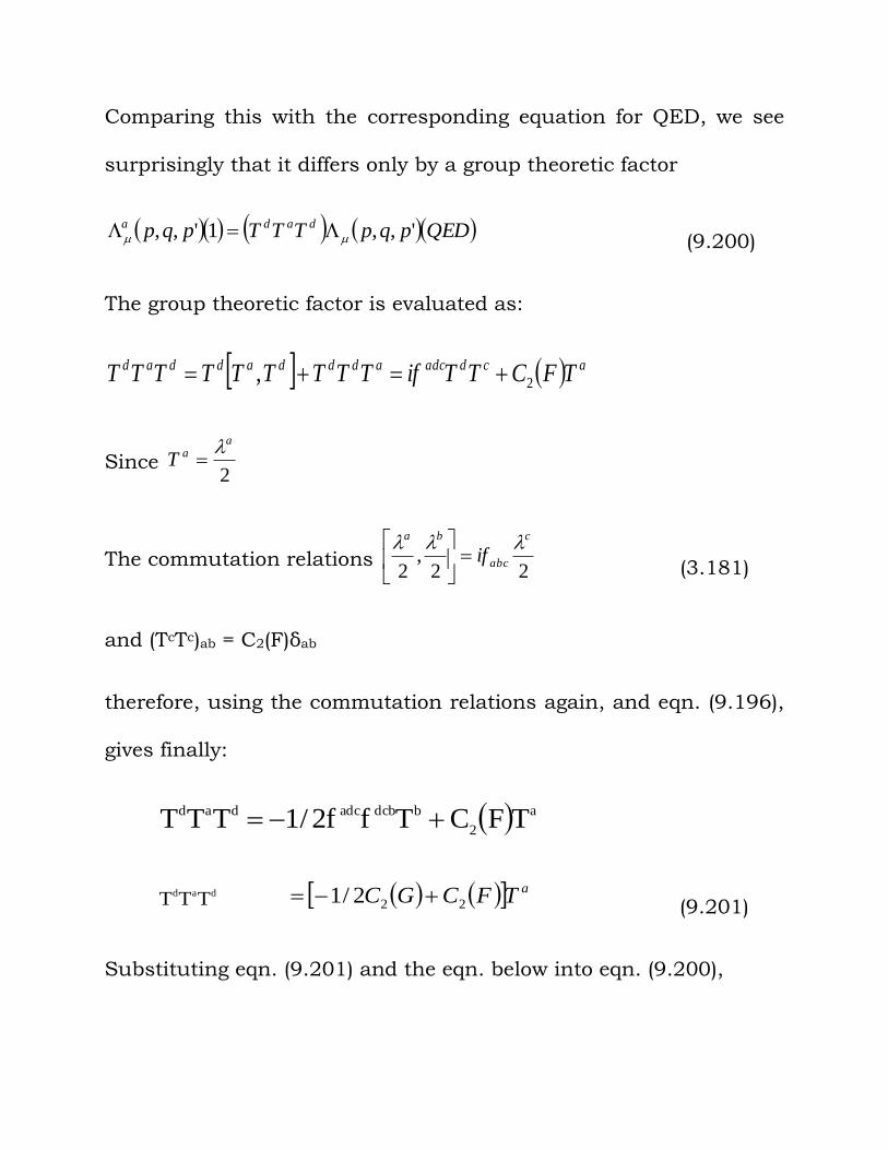
Fig. 9.21: Correction to the quark-gluon vertex involving the 3-

gluon vertex

The contribution in Fig. 9.20 to the vertex function is

1',,2/2 pqpigcd

ad

2

32/2 .'2 k

igT

mkp

iT

mkp

iT

kdig ib

d

ji

a

ij

d

d

dd

Comparing this with the corresponding equation for QED, we see

surprisingly that it differs only by a group theoretic factor

QEDpqpTTTpqp dada ',,1',, (9.200)

The group theoretic factor is evaluated as:

acdadcadddaddad TFCTTifTTTTTTTTT 2,

Since 2

aaT

The commutation relations 22

,2

c

abc

ba

if

(3.181)

and (TcTc)ab = C2(F)δab

therefore, using the commutation relations again, and eqn. (9.196),

gives finally:

a

2

bdcbadcdad TFCTff2/1TTT

dad TTT aTFCGC 222/1 (9.201)

Substituting eqn. (9.201) and the eqn. below into eqn. (9.200),

2

2)1(

8',,

gpqp

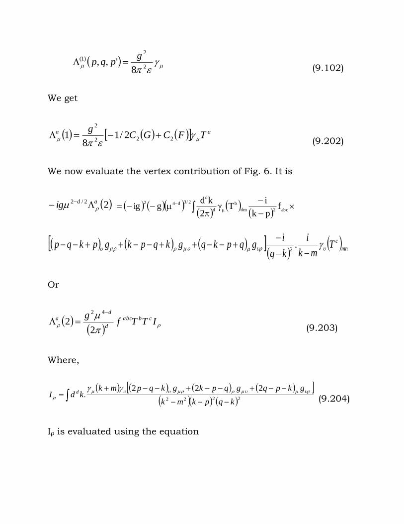
(9.102)

We get

aa TFCGCg

222

2

2/18

1 (9.202)

We now evaluate the vertex contribution of Fig. 6. It is

22/2 adig

abc2dm

b

d

d2/3d42

fpk

iT

2

kdgig

mn

cTmk

i

kq

igqpkqgkqpkgpkqp

.

2

Or

ITTf

g cbabc

d

da

22

42

(9.203)

Where,

2222

222.

kqpkmk

gkpqgqpkgkqpmkkdI d

(9.204)

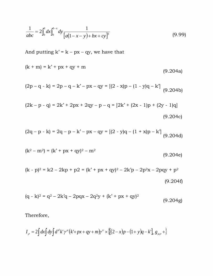
Iρ is evaluated using the equation

31

0

1

0 1

12

1

cybxyxadydx

abc

x

(9.99)

And putting k’ = k – px – qy, we have that

(k + m) = k’ + px + qy + m (9.204a)

(2p – q - k) = 2p – q – k’ – px – qy = [(2 - x)p – (1 - y)q – k’] (9.204b)

(2k – p - q) = 2k’ + 2px + 2qy – p – q = [2k’ + (2x - 1)p + (2y - 1)q]

(9.204c)

(2q – p - k) = 2q – p – k’ – px – qy = [(2 - y)q – (1 + x)p – k’] (9.204d)

(k2 – m2) = (k’ + px + qy)2 – m2 (9.204e)

(k - p)2 = k2 – 2kp + p2 = (k’ + px + qy)2 – 2k’p – 2p2x – 2pqy + p2

(9.204f)

(q - k)2 = q2 – 2k’q – 2pqx – 2q2y + (k’ + px + qy)2 (9.204g)

Therefore,

gkqypxmqypxkkddydxI d '12''2

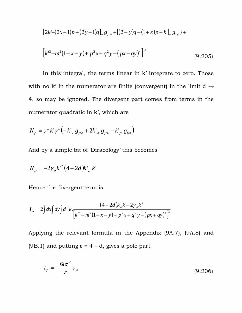
}'121212'2 gkpxqygqypxk

322222 1'

qypxyqxpyxmk (9.205)

In this integral, the terms linear in k’ integrate to zero. Those

with no k’ in the numerator are finite (convergent) in the limit d →

4, so may be ignored. The divergent part comes from terms in the

numerator quadratic in k’, which are

gkgkgkkN v ''2''

And by a simple bit of ‘Diracology’ this becomes

''24'2 2 kkdkN

Hence the divergent term is

322222

2

1

224.2

qypxyqxpyxmk

kkkdkddydxI d

Applying the relevant formula in the Appendix (9A.7), (9A.8) and

(9B.1) and putting ε = 4 – d, gives a pole part

26iI

(9.206)

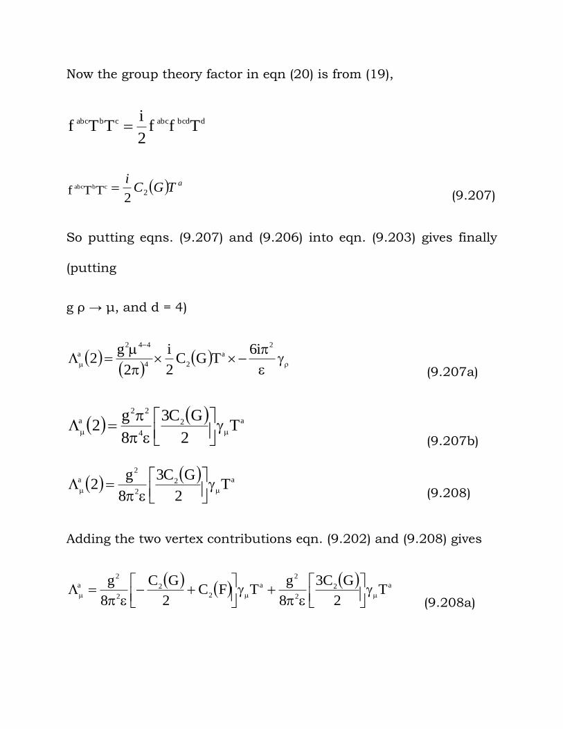
Now the group theory factor in eqn (20) is from (19),

dbcdabccbabc Tff2

iTTf

cbabc TTf aTGCi

22

(9.207)

So putting eqns. (9.207) and (9.206) into eqn. (9.203) gives finally

(putting

g ρ → , and d = 4)

2

a

24

442

a i6TGC

2

i

2

g2

(9.207a)

a2

4

22

a T2

GC3

8

g2

(9.207b)

a2

2

2

a T2

GC3

8

g2

(9.208)

Adding the two vertex contributions eqn. (9.202) and (9.208) gives

T

2

G3C

8

gTFC

2

GC

8

g a2

2

2

a

2

2

2

2

a

(9.208a)

a

2

3

282

22

2

2aTFC

GCGCg

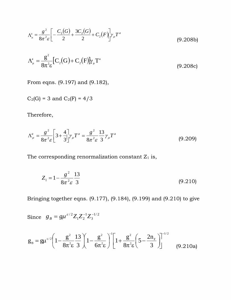
(9.208b)

TFCGC8

g a

222

2

a

(9.208c)

From eqns. (9.197) and (9.182),

C2(G) = 3 and C2(F) = 4/3

Therefore,

aaa Tg

Tg

3

13

83

43

8 2

2

2

2

(9.209)

The corresponding renormalization constant Z1 is,

3

13

81

2

2

1

gZ

(9.210)

Bringing together eqns. (9.177), (9.184), (9.199) and (9.210) to give

Since 2/1

3

1

21

2/ ZZZggB

2/1

F

2

21

2

2

2

2

2/

B3

n25

8

g1

6

g1

3

13

8

g1gg

(9.210a)

3

n

2

5

8

g1

3

4

8

g1

3

13

8

g1gg F

2

2

2

2

2

2

2/

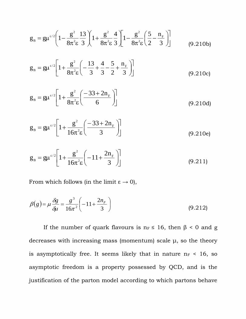
B

(9.210b)

3

n

2

5

3

4

3

13

8

g1gg F

2

2

2/

B

(9.210c)

6

n233

8

g1gg F

2

2

2/

B

(9.210d)

3

n233

16

g1gg F

2

2

2/

B

(9.210e)

3

n211

16

g1gg F

2

2

2/

B

(9.211)

From which follows (in the limit ε → 0),

3

211

16 2

3

Fnggg

(9.212)

If the number of quark flavours is nF ≤ 16, then β < 0 and g

decreases with increasing mass (momentum) scale , so the theory

is asymptotically free. It seems likely that in nature nF < 16, so

asymptotic freedom is a property possessed by QCD, and is the

justification of the parton model according to which partons behave

almost like free particles when interacting at high momentum

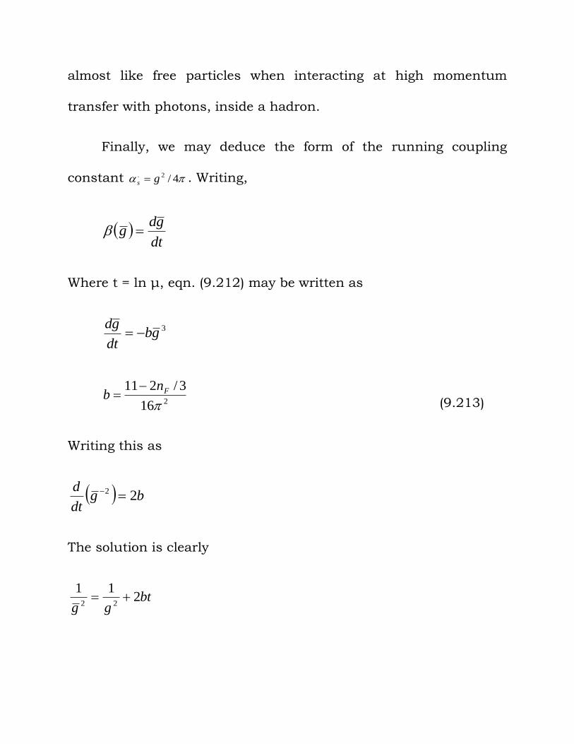
transfer with photons, inside a hadron.

Finally, we may deduce the form of the running coupling

constant 4/2. gs . Writing,

dt

gdg

Where t = ln , eqn. (9.212) may be written as

3gb

dt

gd

216

3/211

Fnb

(9.213)

Writing this as

bgdt

d22

The solution is clearly

btgg

211

22

2

2

2

211

g

btg

g

2

22

21 btg

gg

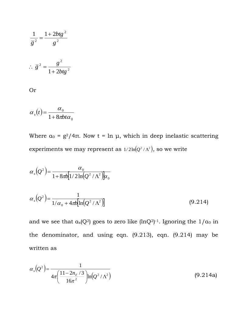
Or

0

0

81

btts

Where α0 = g2/4 . Now t = ln , which in deep inelastic scattering

experiments we may represent as 22 /ln2/1 Q , so we write

0

22

02

/ln2/181

QbQs

22

0

2

/ln4/1

1

QbQs

(9.214)

and we see that αs(Q2) goes to zero like (lnQ2)-1. Ignoring the 1/α0 in

the denominator, and using eqn. (9.213), eqn. (9.214) may be

written as

22

2

2

/ln16

3/2114

1

Qn

QF

s

(9.214a)

22

2

/ln4

3/211

1

Qn

QF

s

(9.214b)

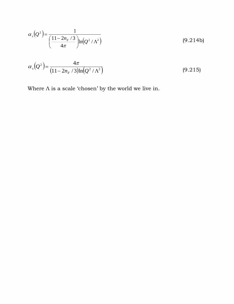
22

2

/ln3/211

4

QnQ

F

s

(9.215)

Where is a scale ‘chosen’ by the world we live in.

CONCLUSION

The power counting formular for the superficial degree of

divergence of Feynman diagrams in QED is derived and primitively

divergent diagrams is isolated.

The electron self energy, vacuum polarization and vertex graph are

evaluated using dimensional regularization.

By explicit calculation of the relevant Feynman diagrams, QCD is

shown to be asymptotically free if the numbers of quark flavours is

less than 16.

REFERENCES

[1]. Gross D.J. (1973). Asymptotically free guage theories I, Phy Rev D, Vol 8, Number 10.

[2]. Hateld, B. (1992). Quantum Field Theory of Point Particles and Strings, Volume 75 of Frontiers in Physics. Addison-Wesley Publishing Company Advanced Book Program, Redwood City, CA.

[3]. Banerjee, H. (1980). Chiral Anomalies in Field Theories, S. N. Bose National Centre for Basic Sciences Salt Lake, India.

[5]. t’Hooft G. and Veltman N. (1972). Regularisation and renormalization of guage fields, Nuclear physics B44, pp 189-213, North publishing company.

[4]. Taylor, J.C.(1976). Gauge Theories of Weak Interactions. Cambridge University Press.

[6]. Pauli W. and Villars F. (1949). On the invariant regularization in relativistic quantum theory, Review Modern Physics, Vol. 21, Number 3.

[7]. Peskin, M.E. and Schr¨oder, D.V. (1995). An introduction to quantum field theory. Westview Press.