Dimensional crossover in anisotropic Kondo lattices

IOP PUBLISHING JOURNAL OF PHYSICS: CONDENSED MATTER

J. Phys.: Condens. Matter 19 (2007) 406203 (10pp) doi:10.1088/0953-8984/19/40/406203

Dimensional crossover in anisotropic Kondo lattices

D Reyes1 and M A Continentino2

1 Centro Brasileiro de Pesquisas Fısicas—Rua Dr Xavier Sigaud, 150-Urca, 22290-180, RJ, Brazil2 Instituto de Fısica, Universidade Federal Fluminense, Campus da Praia Vermelha, Niteroi, RJ,24.210-340, Brazil

E-mail: [email protected] and [email protected]

Received 6 July 2007, in final form 15 August 2007Published 11 September 2007Online at stacks.iop.org/JPhysCM/19/406203

AbstractDimensional crossover in the Kondo necklace model is analyzed using thebond-operator method at zero and finite temperatures. Explicit relationsdescribing quasi-two-dimensional properties are obtained by asymptoticallysolving the resulting equations. The crossover from two dimensions (2d) tothree dimensions (3d) is investigated, turning on the electronic hopping (t⊥)of conduction electrons between different planes. In order to give continuityto our analysis, both cases of crossover, quasi-three-dimensional (q3d) andquasi-one-dimensional (q1d), are also investigated. The phase diagram as afunction of temperature T , J/t‖ and t⊥/t‖, where t‖ is the hopping within theplanes, is calculated. Unusual reentrant behavior in the temperature-dependentantiferromagnetic critical line is found close to two dimensions. Near theisotropic three-dimensional quantum critical point the critical line is describedby a standard power law with a square root dependence on the distance to thequantum critical point.

(Some figures in this article are in colour only in the electronic version)

1. Introduction

Dimensionality plays a central role in strongly correlated electron systems (SCES) [1].For instance, explanations based on two-dimensional (2d) theories in the neighborhoodof a quantum critical point (QCP) [2–7] have been proposed to explain significantunsolved problems in SCES, such as non-Fermi liquid (NFL) behavior and high-temperaturesuperconductivity. But the real materials to which these ideas have been applied are usuallyrendered three dimensional (3d) by a finite electronic coupling between their component layers;a 2d-QCP has not been experimentally observed in any bulk 3d system, and mechanismsfor dimensional reduction have remained the subject of theoretical conjecture [8, 9]. Thusthe very notion of dimensionality can be said to acquire an ‘emergent’ nature: although theindividual particles move on a three-dimensional lattice, their collective behavior occurs inlower-dimensional space.

0953-8984/07/406203+10$30.00 © 2007 IOP Publishing Ltd Printed in the UK 1

J. Phys.: Condens. Matter 19 (2007) 406203 D Reyes and M A Continentino

Specifically in heavy-fermion (HF) materials, there have already been diverse theorieswhich propose that quasi-two-dimensional (q2d) systems play a central role in theunderstanding of anomalous behaviors near a magnetic QCP. Several theories were formulatedto explain their unusual properties [10–12]. In this context the spin-density wave(SDW) [11, 12] theory as well as the local quantum critical description [13] can accountfor the logarithmically divergent specific heat coefficients and quasi-linear resistivities onlyif the spin fluctuations are q2d. The hypothesis that HF materials involve decoupled layersof spins motivates a search for a mechanism that can generate a q2d environment for the spinfluctuations out of a metal that is manifestly three dimensional. One such frequently citedmechanism is geometric anisotropy. Here, the idea is that turning on the hopping betweenplanes t⊥ leads magnetic long-range order (LRO) at finite temperatures. In this paper, we usethe Kondo necklace model [14] as a simple Hamiltonian to explore this line of reasoning. Thebasic aim of our paper is not to examine whether inter-layer coupling is relevant or irrelevant atthe QCP but rather to examine whether anisotropy can set up an environment in which the inter-layer coupling is sufficiently weak for us to consider the system to be quasi-two dimensional inall its properties.

The anisotropic Kondo necklace model (AKNM) is given by

H = t‖∑

i,δ1

(τ xi τ

xi+δ1

+ τyi τ

yi+δ1

)+ t⊥∑

i,δ2

(τ xi τ

xi+δ2

+ τyi τ

yi+δ2

)+ J∑

i

Si · τ i , (1)

where τi and Si are independent sets of spin-1/2 Pauli operators, representing the conductionelectron spins and localized spin operators, respectively. δ1(δ2) is the difference betweenlattice vectors of the in-plane (inter-plane) nearest-neighbor sites. t‖ is the hopping within theplanes and t⊥ that between them. The last term is the magnetic interaction between conductionelectrons and localized spins via the coupling J .

The plan of the paper is the following. In section 2 we set up the bond-operator formalism.In section 3 we describe the antiferromagnetic (AF) ordered state solving the anisotropic Kondonecklace Hamiltonian via the Green’s function method; also we show the order parameters atfinite temperatures. Section 4 discusses the Neel line in the AKNM. Using the results obtainedin the previous section the thermodynamic phase transition and phase diagrams are discussedin section 5 for both cases, the q2d and q3d AKNM. The case ξ � 1 that corresponds to d = 1will be shown only to give continuity to our analysis. Also the reentrance phenomenon, i.e. twosuccessive transitions for certain parameter values, is analyzed. Finally, in section 6 we givethe conclusions of our paper.

2. Bond-operators formalism

The bond-operator mean-field approach [15] is basically a strong coupling approximation inJ . The spins between layers dominantly form singlets and the density of triplets is ‘low’ (thisassumption will allows one to neglect triplet–triplet interaction). For two S = 1

2 spins, Sachdevand Bhatt [15] introduced four creation operators to represent the four states in Hilbert space.This basis can be created out of the vacuum by singlet |s〉 and triplet |tα〉 = t†

α |0〉 (α = x, y, z)operators. In terms of these triplet and singlet operators the localized and conduction electronspin operators are given by

Si,α = 12

(s†

i ti,α + t†i,αsi − iεαβγ t†

i,β ti,γ

),

τi,α = 12

(−s†

i ti,α − t†i,αsi − iεαβγ t†

i,β ti,γ

),

(2)

where α, β and γ take the values x , y, z, repeated indices are summed over, and ε is the totallyantisymmetric Levi–Civita tensor. The restriction that the physical states are either singlets or

2

J. Phys.: Condens. Matter 19 (2007) 406203 D Reyes and M A Continentino

triplets leads to the constraint s†s + ∑α t†α tα = 1. Moreover, the singlet and triplet operators

at each site satisfy bosonic commutation relations [s, s†] = 1, [tα, t†β] = δα,β , [s, t†

α] = 0.Substituting the operator representation of spins defined in equation (2) into the originalHamiltonian equation (1) and considering the commutation relations, we obtain

H = H0 + H1 + H2

where

H0 = J

4

∑

i

(−3s†

i si + t†i,x ti,x + t†

i,yti,y + t†i,z ti,z

)

+∑

i

μi

(s†

i si + t†i,x ti,x + t†

i,yti,y + t†i,z ti,z − 1

),

H1 = t‖4

∑

i,δ1;α

(s†

i s†i+δ1

ti,αti+δ1,α+ s†

i si+δ1ti,αt†

i+δ1,α

)

− t‖4

∑

i,δ1;α

(t†i,z t†

i+δ1,zti,αti+δ1,α

− t†i,z ti+δ1,z

ti,α t†i+δ1,α

+ h.c.),

H2 = t⊥4

∑

i,δ2;α

(s†

i s†i+δ2

ti,αti+δ2,α+ s†

i si+δ2ti,αt†

i+δ2,α

)

− t⊥4

∑

i,δ2;α

(t†i,z t†

i+δ2,zti,α ti+δ2,α

− t†i,z ti+δ2,z

ti,αt†i+δ2,α

+ h.c.).

(3)

Here α = x, y. H0 represents the interaction between spins S and τ in the site i and theconstraint s†s+t†

i,x ti,x +t†i,yti,y+t†

i,z ti,z = 1 is implemented through the local chemical potentialsμi . H1, H2, are terms associated with the hopping t‖ and t⊥, respectively. As argued before,we neglect triplet–triplet interactions [19].

3. Antiferromagnetic ordered phase

The Hamiltonian above, at half filling, can be simplified using a mean-field decoupling [20].Relying on the nature of the strong coupling limit (t/J ) → 0 we take 〈s†

i 〉 = 〈si 〉 = s. Next,to describe the condensation of one local Kondo spin triplet tk,x on the AF reciprocal vectorQ = (π/a, π/a, π/a), we introduce: tk,x = √

Ntδk,Q + ηk,x corresponding to fixing theorientation of the localized spins along the x direction. The quantity t is the mean value of thex-component spin triplet in the ground state and ηk,x represents the fluctuations. Finally thetranslation invariance of the problem implies that we may assume the local chemical potentialas a global one.

Making approximations already used in the bond-operator formalism [16, 17] and afterperforming a Fourier transformation of the boson operators, we get

Hm f = N

(−3

4Js2 + μs2 − μ

)+

(J

4+ μ

) ∑

k

t†k,z tk,z

+(

J

4+ μ− 1

2s2(t‖ Z‖ + t⊥Z⊥)

)Nt2

+∑

k

[�kη

†k,xηk,x + Dk

(η

†k,xη

†−k,x + ηk,xη−k,x

)]

+∑

k

[�kt†

k,ytk,y + Dk

(t†k,yt†

−k,y + tk,yt−k,y

)], (4)

with �k = ω0 + 2Dk, λ(k)‖ = cos kx + cos ky , �k = 14 t‖s2λ(k)‖, λ(k)⊥ = cos kz ,

�′k = 1

4 t⊥s2λ(k)⊥, Dk = �k + �′k, N is the number of lattice sites, Z‖ = 4 is the total

3

J. Phys.: Condens. Matter 19 (2007) 406203 D Reyes and M A Continentino

number of the nearest neighbors in planes and Z⊥ = 2 is the number of the nearest neighborsbetween planes. The wavevectors k are taken in the first Brillouin zone and the lattice spacingwas assumed to be unity. We have considered for simplicity a cubic lattice.

Now we obtain the free energy; for that, we shall employ the equation of motion methodusing the Green’s functions and thus to obtain the thermal averages 〈Hm f 〉 = U . So the thermalaverages of the singlet and triplet correlation functions are obtained from

〈〈γk,α; γ †k,α〉〉ω = 1

2π

ω +�k

ω2 − ω2k

, 〈〈tk,z; t†k,z〉〉ω = 1

2π

1

ω − ω0, (5)

where γ = η, (t) for α = x, (y). The poles of the Green’s functions determine the excitationenergies of the system as ω0 = ( J

4 +μ), which is the dispersionless spectrum of the longitudinal

spin triplet states and ωk = ±√�2

k − (2Dk)2 that correspond to the excitation spectrum ofthe transverse spin triplet states for both branches ωx = ωy . Then, we can stress that thecontribution of the term k = Q for the free energy from the bosons tk,x will depend only on theaverage value t in the expression and not on the energy spectrum of the bosons. Consequentlythe Green’s function for both α = x and y is the same. Solving the coupled equations of motionobtained for the Green’s function propagators we obtain

U = 〈Hm f 〉 = ε0 + ω0

2

∑

k

(coth

βω0

2− 1

)+

∑

k

ωk

(coth

βωk

2− 1

), (6)

where

ε0 = N

(−3

4Js2 + μs2 − μ

)+ N

(J

4+ μ− 1

2s2(t‖ Z‖ + t⊥Z⊥)

)t2 +

∑

k

(ωk − ω0), (7)

is the ground state energy of the system, β = 1/kBT , s and t being the singlet and triplet orderparameters, respectively.

Considering the above equation (6) and that the entropy of free bosons is S =kB

∑k[(n(ωk)+ 1) ln(n(ωk)+ 1)− n(ωk) ln(n(ωk))], the free energy F = U − T S is trivially

obtained as

F = ε0 − 2

β

∑

k

ln[1 + n(ωk)] − N

βln[1 + n(ω0)], (8)

where n(ω) = 12 (coth βω

2 − 1) is the occupation factor for bosons. Since the parameters is always nonzero [19, 18] and t = 0 in the antiferromagnetic phase, we minimizethe ground state energy with respect to t to find μ = t‖s2/y − J/4, and consequentlyωk = 1

y t‖s2√

1 + y(λ(k)‖ + ξλ(k)⊥) where ξ = t⊥/t‖ is the real spatial anisotropy ratiobetween the hopping along different directions and y = 1/(2 + ξ). Then, we can calculate theother parameters s2 = s2(T ) and t2 = t2

(T ) minimizing the free energy equation (8). Using(∂ε/∂μ, ∂ε/∂s) = (0, 0), we can easily get the following saddle-point equations:

s2 = 1 + J

t‖y

2− 1

2N

∑

k

√1 + y(λ(k)‖ + ξλ(k)⊥) coth

βωk

2− ς,

t2 = 1 − J

t‖y

2− 1

2N

∑

k

1√1 + y(λ(k)‖ + ξλ(k)⊥)

cothβωk

2− ς,

(9)

where ς = 14 (coth βω0

2 − 1). Generally the equations for s and t in equation (9) should besolved and at ξ = 0, (ξ = 1) the results of [20] for 2d (3d) are recovered. For J/t‖ > (J/t‖)c,triplet excitations remain gapped and at J/t‖ < (J/t‖)c the ground state has both condensationof singlets and triplets at the antiferromagnetic wavevector Q = (π, π, π). Then, the QCP atT = 0, (J/t)c separates an antiferromagnetic long-range ordered phase from a gapped spin

4

J. Phys.: Condens. Matter 19 (2007) 406203 D Reyes and M A Continentino

liquid phase. For finite temperatures, the condensation of singlets s occurs at a temperaturescale which, to a first approximation, tracks the exchange J . The energy scale below whichthe triplet excitations condense is given by the Neel temperature (TN) which is calculated in thenext section near the AF magnetic instability.

4. Neel temperature in the AKNM

The Neel line giving the finite temperature instability of the antiferromagnetic phase forJ/t‖ < (J/t‖)c is obtained as the line in the T versus (J/t‖) plane at which t vanishes (t = 0).Thereby from equation (9) we have

J

t‖= 2

y

(1 − 1

2N

∑

k

1√1 + y(λ(k)‖ + ξλ(k)⊥)

cothβωk

2+ ς

). (10)

This expression defines the boundary of the AF state. Consequently the QCP is obtainedmaking T = 0 in equation (10), then we get

(J

t‖

)

c

= 2

y

(1 − 1

2N

∑

k

1√1 + y(λ(k)‖ + ξλ(k)⊥)

), (11)

where y = 1/(2 + ξ) as defined before. Because g = |(J/t‖)c − (J/t‖)| measures the distanceto the QCP we finally obtain

|g| = 1

y N

∑

k

1√1 + y(λ(k)‖ + ξλ(k)⊥)

(coth

βωk

2− 1

)+ 2ς

y. (12)

4.1. Numerical results at T = 0

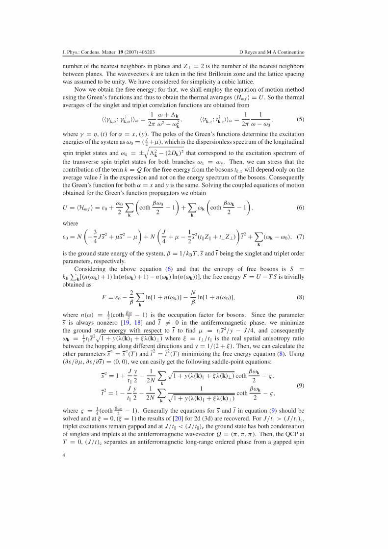
In order to find the AF boundary at T = 0 we are going to calculate as the QCP varies from 2dto 3d, i.e. as we turn on ξ . Our numerical task consists in evaluating, at various ξ , the quantumcritical point given by equation (11). For this purpose we first consider the isotropic cases,i.e. ξ = 1 (3d) with t‖ = t⊥ = t , and ξ = 0 (2d) where t‖ = t and t⊥ = 0. Thereby weeasily obtain J/t ≈ 1.4409 (J/t ≈ 2.6611) in 2d (3d) in agreement with previous works inthe KNM [19] as well as KLM [18]. In figure 1 we have plotted the coupling strength (J/t‖)cversus the anisotropy at 1 − ξ for different ξ ∈ [0,1]. The inset shows the log–log plot of gversus ξ close to d = 2 (ξ ∈ [0, 0.1], g = |(J/t‖)c − (J/t‖)c2d | and (J/t‖)c2d ≈ 1.4409). Theline fit yields g ∝ ξ 1.8.

In summary, in this section we have established the essential expression, equation (12),for finding the Neel temperature as a function of g and ξ as well as the QCP dependenceon the anisotropy ξ . In the next section we are going to use the calculations above toinvestigate analytically if there is thermodynamic phase transition when inter-plane hoppingt⊥ is turned on.

5. Analytical results for finite temperature

In this section we are going to calculate analytically the Neel critical line for both the q2d(ξ � 1) and q3d (ξ ≈ 1) AKNM. The case ξ � 1 that corresponds to d = 1 will beshown only to give continuity to our analysis. All the calculations will be done considering twoessential approximations: (i) the system is close to a magnetic instability; (ii) the temperatureregion where the Neel line will be found will be lower than the Kondo temperature (TK).

5

J. Phys.: Condens. Matter 19 (2007) 406203 D Reyes and M A Continentino

Figure 1. Zero temperature phase diagram showing the line of quantum phase transitions (J/t‖)cas a function of the anisotropy parameter 1 − ξ . Also shown is the AF border (J/t‖)c at2d (2d-QCP ≈ 1.4409) and 3d (3d-QCP ≈ 2.6611). The points were obtained by solvingequation (11). The inset shows the log–log plot of g versus ξ close to d = 2 (ξ ∈ [0, 0.1],g = |(J/t‖)c − (J/t‖)c2d | and (J/t‖)c2d ≈ 1.4409). The line fit yields g ∝ ξ1.8.

We will start expanding k close to the wavevector Q = (π, π, π) associated with theantiferromagnetic instability, so we get

λ(k)‖ = −2 + k2‖

2+ O(k4

‖),

λ(k)⊥ = −1 + k2z

2+ O(k4

z ).

(13)

This yields the spectrum of transverse spin triplet excitations as

ωk = ω0

√1 + y(λ(k)‖ + ξλ(k)⊥) ≈ ω0

√y

2(k2

‖ + ξk2z ), (14)

where ω0 is the z-polarized dispersionless branch of excitations. Replacing equation (14) inequation (12), and considering that for temperatures kBT � ω0, ς goes to zero faster than thefirst term of equation (12), we obtain

|g| y

2= 1

π2

∫ π

0

∫ π

0

k‖ dk‖ dkz√y2 (k

2‖ + ξk2

z )

(coth

βωk

2− 1

). (15)

For ξ = 0 the integral above diverges, excluding long-range order at finite temperatures in twodimensions in accord with the Mermim–Wagner theorem [21]. On the other hand, when ξ = 1,the in-plane interaction equals the inter-plane coupling (t⊥ = t‖) and we have a pure 3d KNMwith TN ∝ √|g| as found in a previous work [20].

5.1. The case ξ � 1

We now demonstrate analytically the appearance of a finite Neel line temperature when a smallhopping t⊥ between planes is turned on. Making a change of variables in equation (15) weobtain

|g| = 1

y2π2α

∫ π

0

(∫ b

a(coth u − 1) du

)dkz, (16)

6

J. Phys.: Condens. Matter 19 (2007) 406203 D Reyes and M A Continentino

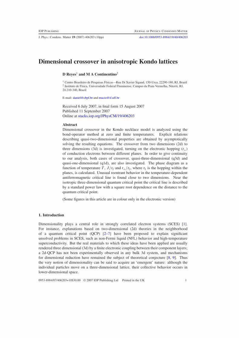
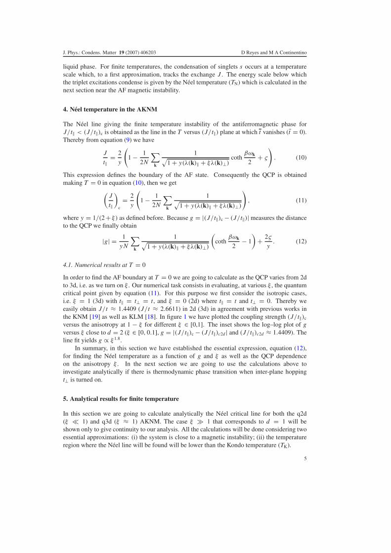
Figure 2. Phase diagram between the temperature as α−1c and J/t‖ for nonzero ξ . We observe

that Neel order arises for an arbitrarily weak inter-plane hopping t⊥ and it increases as ξ increases.2d-QCP shows the zero temperature quantum critical point in 2d (ξ = 0). The interesting featureof this phase diagram is the reentrant behavior for 0.002 < ξ < 0.1. As temperature is lowered, thesystem passes from a disordered paramagnetic phase (with no spontaneous symmetry braking), tothe antiferromagnetic phase, and back to the disordered phase as the temperature is lowered further.

where u = 2α√

y2 (k

2‖ + ξk2

z ), b = 2α√

y(π2 + ξk2z )/2, a = 2α

√ξy/2kz and α = ω0/4kBT .

While each of the Kondo systems has its own energy scale Kondo temperature TK belowwhich the thermodynamic and transport properties are governed by the QCP [22], relevantperturbation which is normally present in real systems introduces another energy scale Tx

where crossover to another regime occurs (for instance, the coherence temperature proposedby Continentino and collaborators [23]). In our case we argue that the Neel temperature regioncan be observed only when Tx/TK � 1. In other words, the Neel region can be observed onlyfor α � 1 (since ω0 tracks J ∼ TK). Thereby, solving equation (16) considering the latter andξ � 1 we get

|g|ξ�1 = 2√ξ + 4

πα

[1 − ln

(2π

√ξα

)]+ O(ξ), (17)

where we took y ≈ (1 − ξ

2 )/2 and the second term in the right-hand side takes into accountthe thermal fluctuations. Equation (17) gives us the Neel line as a function of the distance toQCP g for a small but finite anisotropy ξ and temperatures kBT � ω0, where as said beforeω0 tracks TK. We observe in equation (17) that |g| diverges for ξ = 0, then in two dimensionsthere is no AF ordering above zero temperature. As soon as the dimension of the AKNM isgreater than two, there is a nonzero-temperature phase transition.

In figure 2 we show the phase diagram α−1c = 4kBTN/ω0 as a function of J/t‖ for different

value of ξ between [2×10−3, 10−1]. α−1c is defined as the critical line where Neel order appears.

We observe a reentrance phenomenon that will be discussed in the following subsection. Closeto the isotropic 3d-QCP the system does not display this phenomenon. At this point we canconstruct the phase diagram α−1

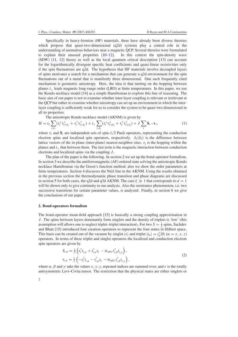
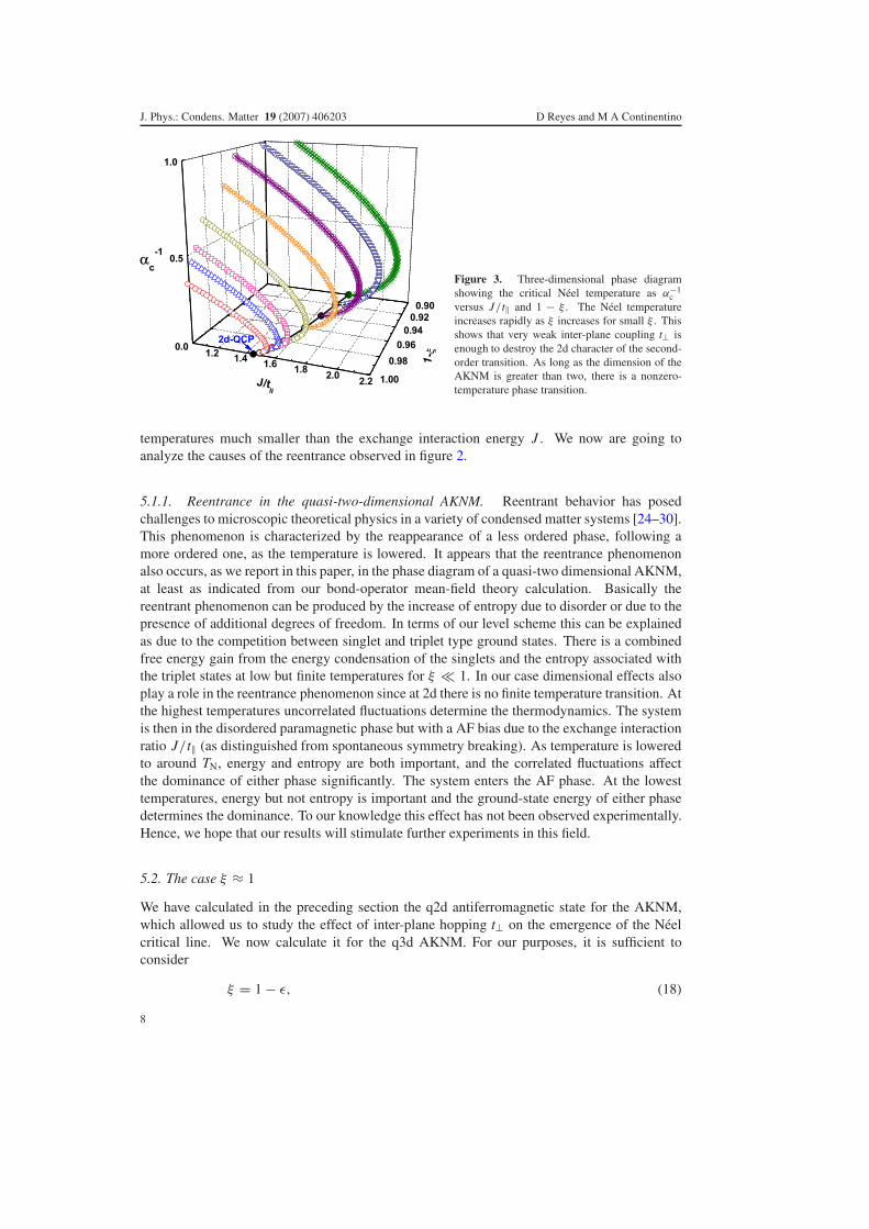
c versus J/t‖ versus 1 − ξ for ξ � 1 considering our analyticaland numerical calculations. This is shown in figure 3, where the boundary line at T = 0 hasbeen calculated using equation (11) and the Neel lines using equation (17).

In summary, in this subsection we have obtained analytically the expression for the Neelline close to the QCP in q2d and we have shown that in fact this line exists for ξ � 1 and

7

J. Phys.: Condens. Matter 19 (2007) 406203 D Reyes and M A Continentino

Figure 3. Three-dimensional phase diagramshowing the critical Neel temperature as α−1

cversus J/t‖ and 1 − ξ . The Neel temperatureincreases rapidly as ξ increases for small ξ . Thisshows that very weak inter-plane coupling t⊥ isenough to destroy the 2d character of the second-order transition. As long as the dimension of theAKNM is greater than two, there is a nonzero-temperature phase transition.

temperatures much smaller than the exchange interaction energy J . We now are going toanalyze the causes of the reentrance observed in figure 2.

5.1.1. Reentrance in the quasi-two-dimensional AKNM. Reentrant behavior has posedchallenges to microscopic theoretical physics in a variety of condensed matter systems [24–30].This phenomenon is characterized by the reappearance of a less ordered phase, following amore ordered one, as the temperature is lowered. It appears that the reentrance phenomenonalso occurs, as we report in this paper, in the phase diagram of a quasi-two dimensional AKNM,at least as indicated from our bond-operator mean-field theory calculation. Basically thereentrant phenomenon can be produced by the increase of entropy due to disorder or due to thepresence of additional degrees of freedom. In terms of our level scheme this can be explainedas due to the competition between singlet and triplet type ground states. There is a combinedfree energy gain from the energy condensation of the singlets and the entropy associated withthe triplet states at low but finite temperatures for ξ � 1. In our case dimensional effects alsoplay a role in the reentrance phenomenon since at 2d there is no finite temperature transition. Atthe highest temperatures uncorrelated fluctuations determine the thermodynamics. The systemis then in the disordered paramagnetic phase but with a AF bias due to the exchange interactionratio J/t‖ (as distinguished from spontaneous symmetry breaking). As temperature is loweredto around TN, energy and entropy are both important, and the correlated fluctuations affectthe dominance of either phase significantly. The system enters the AF phase. At the lowesttemperatures, energy but not entropy is important and the ground-state energy of either phasedetermines the dominance. To our knowledge this effect has not been observed experimentally.Hence, we hope that our results will stimulate further experiments in this field.

5.2. The case ξ ≈ 1

We have calculated in the preceding section the q2d antiferromagnetic state for the AKNM,which allowed us to study the effect of inter-plane hopping t⊥ on the emergence of the Neelcritical line. We now calculate it for the q3d AKNM. For our purposes, it is sufficient toconsider

ξ = 1 − ε, (18)

8

J. Phys.: Condens. Matter 19 (2007) 406203 D Reyes and M A Continentino

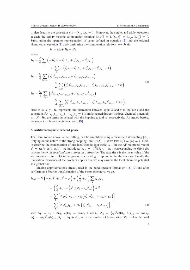
Figure 4. Phase diagram between thetemperature for α−1

c versus J/t‖ forξ ≈ 1. We observe that the Neel line isonly renormalized when the inter-planehopping t⊥ ∼ t‖ . The inset shows thelog–log plot of α−1

c versus g. The Neelline scales like TN ∼ gψ with ψ ≈ 0.5close to the 3d-QCP.

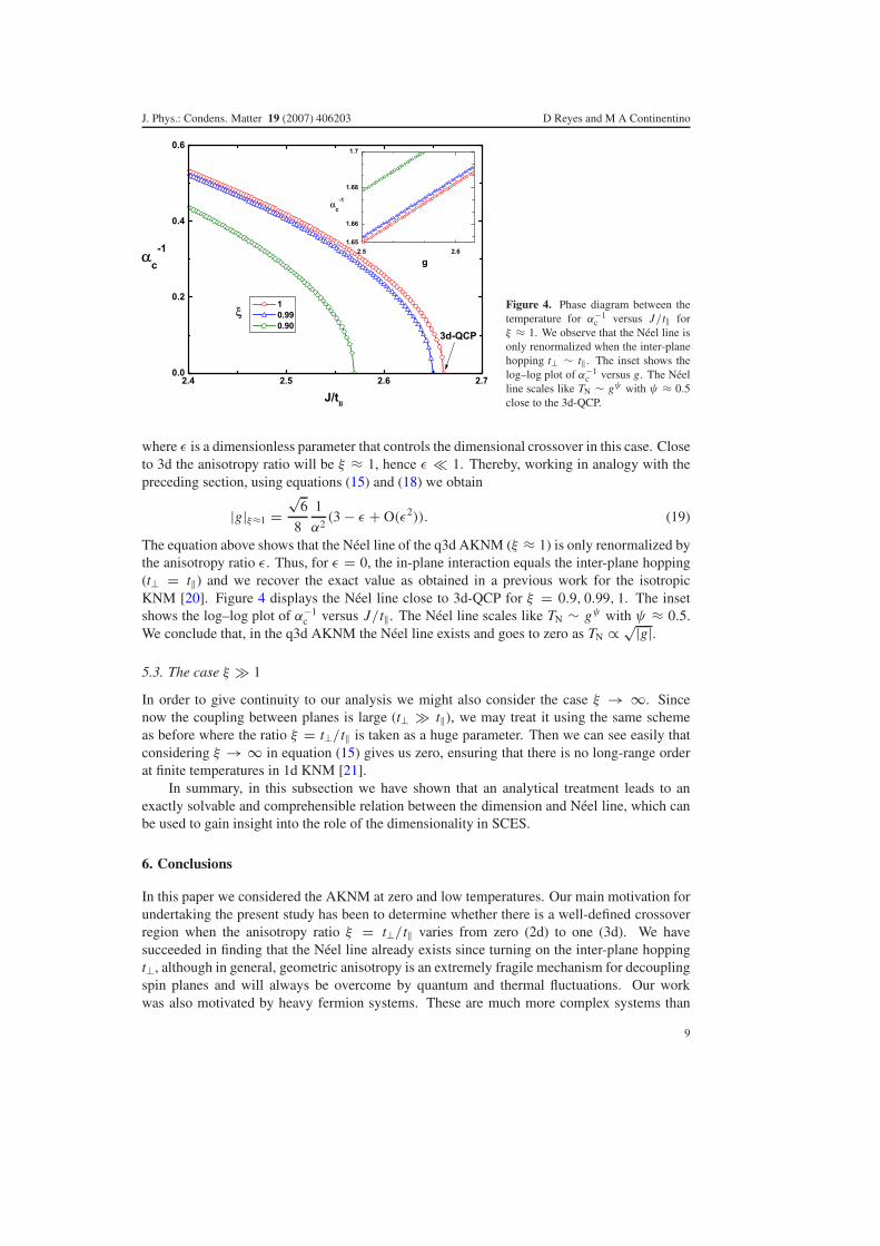
where ε is a dimensionless parameter that controls the dimensional crossover in this case. Closeto 3d the anisotropy ratio will be ξ ≈ 1, hence ε � 1. Thereby, working in analogy with thepreceding section, using equations (15) and (18) we obtain

|g|ξ≈1 =√

6

8

1

α2(3 − ε + O(ε2)). (19)

The equation above shows that the Neel line of the q3d AKNM (ξ ≈ 1) is only renormalized bythe anisotropy ratio ε. Thus, for ε = 0, the in-plane interaction equals the inter-plane hopping(t⊥ = t‖) and we recover the exact value as obtained in a previous work for the isotropicKNM [20]. Figure 4 displays the Neel line close to 3d-QCP for ξ = 0.9, 0.99, 1. The insetshows the log–log plot of α−1

c versus J/t‖. The Neel line scales like TN ∼ gψ with ψ ≈ 0.5.We conclude that, in the q3d AKNM the Neel line exists and goes to zero as TN ∝ √|g|.

5.3. The case ξ � 1

In order to give continuity to our analysis we might also consider the case ξ → ∞. Sincenow the coupling between planes is large (t⊥ � t‖), we may treat it using the same schemeas before where the ratio ξ = t⊥/t‖ is taken as a huge parameter. Then we can see easily thatconsidering ξ → ∞ in equation (15) gives us zero, ensuring that there is no long-range orderat finite temperatures in 1d KNM [21].

In summary, in this subsection we have shown that an analytical treatment leads to anexactly solvable and comprehensible relation between the dimension and Neel line, which canbe used to gain insight into the role of the dimensionality in SCES.

6. Conclusions

In this paper we considered the AKNM at zero and low temperatures. Our main motivation forundertaking the present study has been to determine whether there is a well-defined crossoverregion when the anisotropy ratio ξ = t⊥/t‖ varies from zero (2d) to one (3d). We havesucceeded in finding that the Neel line already exists since turning on the inter-plane hoppingt⊥, although in general, geometric anisotropy is an extremely fragile mechanism for decouplingspin planes and will always be overcome by quantum and thermal fluctuations. Our workwas also motivated by heavy fermion systems. These are much more complex systems than

9

J. Phys.: Condens. Matter 19 (2007) 406203 D Reyes and M A Continentino

the insulating Kondo systems at half-filling presented here. Nevertheless, we believe thatour mechanism for the formation of a q2d Neel line by means of a real spatial anisotropysurvives in the case of more complicated SCES. It emphasizes the need to consider the effectsof dimensionality in a more realistic generalization of the widely accepted views that followfrom Doniach’s Kondo necklace model. We are led to conclude that inter-plane coupling isessential to keep 3d AF ordering at finite temperatures. Therefore there are AF phase transitionsfor ξ > 0 at the Neel temperature TN > 0.

Although the transport properties related to the kinetic energy of conduction electrons arenot quantitatively represented in the Hamiltonian (1), the most essential features of Kondolattices, i.e. the competition between a long-range ordered state and a disordered state is clearlyretained in the model. The qualitative features regarding the stability of the AF phase are welldisplayed in the model and it allows a simple physical interpretation of the phase diagram inanisotropic Kondo lattices. It will be left to a further work to compare our theoretical resultsobtained for the AKNM with both experimental data and different levels of approximationin order to clarify to what extent the estimates of ξ from measured quantities depend on thetheoretical tools used.

Acknowledgments

The authors would like to thank the Brazilian agencies FAPERJ and CNPq for financial support.

References

[1] Reyes D and Continentino M A 2007 Physica B at press[2] Sachdev S 2000 Science 288 475–80[3] Stockert O, von Lohneysen H, Rosch H, Pyka N and Loewenhaupt M 1998 Phys. Rev. Lett. 80 5627–30[4] Si Q, Rabello S, Ingersent K and Smith J L 2001 Nature 413 804–8[5] Mathur N D et al 1998 Nature 394 39–43[6] Senthil T, Vishwanth A, Balents L, Sachdev S and Fisher M P A 2004 Science 303 1490–4[7] Millis A J 1993 Phys. Rev. B 48 7183–96[8] Batista C D and Nussinov Z 2005 Phys. Rev. B 72 045137[9] Xu C and Moore J E 2005 Phys. Rev. B 72 064455

[10] Continentino M A 1993 Phys. Rev. B 47 11587[11] Moriya T and Takimoto T 1995 J. Phys. Soc. Japan 64 960[12] Hertz J A 1976 Phys. Rev. B 14 1165[13] Si Q, Rabello R, Ingersent K and Smith J 2001 Nature 413 804[14] Doniach S 1977 Physica B 91 231[15] Sachdev S and Bhatt R N 1990 Phys. Rev. B 41 9323[16] Gopalan S, Rice T M and Sigrist M 1994 Phys. Rev. B 49 8901[17] Normand B and Rice T M 1996 Phys. Rev. B 54 7180[18] Jurecka C and Brenig W 2001 Phys. Rev. B 64 092406[19] Zhang G-M, Gu Q and Yu L 2000 Phys. Rev. B 62 69[20] Reyes D and Continentino M A 2007 Phys. Rev. B 76 075114[21] Mermin N D and Wagner H 1966 Phys. Rev. Lett. 17 1133[22] Continentino M A 2001 Scaling in Many-Body Systems (Singapore: World Scientific)[23] Continentino M A, Japiasu G and Troper A 1989 Phys. Rev. B 39 9734[24] Fertig J G and Maple M B 1974 Solid State Commun. 15 453[25] Simanek E 1981 Phys. Rev. B 23 5762[26] Cladis P E 1975 Phys. Rev. Lett. 35 48[27] Tinh N H, Hardouin F and Destrade C 1982 J. Physique 43 1127[28] Indekeu O J and Berker A N 1986 Phys. Rev. A 33 1158[29] Manheimer A M, Bhagat S M and Chem H S 1982 Phys. Rev. B 26 456[30] Vasconcelos dos Santos R J, Sa Barreto F C and Coutinho S 1990 J. Phys. A: Math. Gen. 23 2563

10