DEPT. OF ECE, MRCET DSP LAB MANUAL DIGITATL SIGNAL PROCESSING LABORATORY MANUAL B.Tech (III Year-II Sem) (2020-2021) Prepared by Mrs.N.Saritha, Assistant Professor Mr.K.L.N.Prasad, Assistant Professor DEPARTMENT OF ELECTRONICS AND COMMUNICATIONS ENGG. MALLA REDDY COLLEGE OF ENGINEERING & TECHNOLOGY (Autonomous Institution – UGC, Govt. of India) (Affiliated to JNTU, Hyderabad, Approved by AICTE - Accredited by NBA & NAAC – ‘A’ Grade - ISO 9001:2015 Certified) Maisammaguda, Dhulapally (Kompally), Secunderabad – 500100, Telangana State, India www.mrcet.ac.in

Welcome message from author
This document is posted to help you gain knowledge. Please leave a comment to let me know what you think about it! Share it to your friends and learn new things together.
Transcript
DEPT. OF ECE, MRCET DSP LAB MANUAL
DIGITATL SIGNAL PROCESSING LABORATORY MANUAL
B.Tech (III Year-II Sem)
(2020-2021)
Prepared by
Mrs.N.Saritha, Assistant Professor Mr.K.L.N.Prasad, Assistant Professor
DEPARTMENT OF ELECTRONICS AND COMMUNICATIONS ENGG.
MALLA REDDY COLLEGE OF ENGINEERING & TECHNOLOGY
(Autonomous Institution – UGC, Govt. of India) (Affiliated to JNTU, Hyderabad, Approved by AICTE - Accredited by NBA & NAAC – ‘A’ Grade - ISO
9001:2015 Certified) Maisammaguda, Dhulapally (Kompally), Secunderabad – 500100, Telangana State, India
www.mrcet.ac.in

ELECTRONICS & COMMUNICATION ENGINEERING
VISION To evolve into a center of excellence in Engineering Technology through creative and innovative
practices in teaching-learning, promoting academic achievement & research excellence to produce
internationally accepted competitive and world class professionals.
MISSION To provide high quality academic programmes, training activities, research facilities and opportunities
supported by continuous industry institute interaction aimed at employability, entrepreneurship,
leadership and research aptitude among students.
QUALITY POLICY Impart up-to-date knowledge to the students in Electronics & Communication area to make
them quality engineers.
Make the students experience the applications on quality equipment and tools.
Provide systems, resources and training opportunities to achieve continuous improvement.
Maintain global standards in education, training and services.

PROGRAMME EDUCATIONAL OBJECTIVES (PEOs)
PEO1: PROFESSIONALISM & CITIZENSHIP
To create and sustain a community of learning in which students acquire knowledge and
learn to apply it professionally with due consideration for ethical, ecological and economic
issues.
PEO2: TECHNICAL ACCOMPLISHMENTS
To provide knowledge based services to satisfy the needs of society and the industry by
providing hands on experience in various technologies in core field.
PEO3: INVENTION, INNOVATION AND CREATIVITY
To make the students to design, experiment, analyze, interpret in the core field with the help
of other multi disciplinary concepts wherever applicable.
PEO4: PROFESSIONAL DEVELOPMENT
To educate the students to disseminate research findings with good soft skills and become a
successful entrepreneur.
PEO5: HUMAN RESOURCE DEVELOPMENT
To graduate the students in building national capabilities in technology, education and
research.
PROGRAMME SPECIFIC OBJECTIVES (PSOs)
PSO1 To develop a student community who acquire knowledge by ethical learning and fulfill the societal and industry needs in various technologies of core field.
PSO2 To nurture the students in designing, analyzing and interpreting required in research and development with exposure in multi disciplinary technologies in order to mould them as successful industry ready engineers/entrepreneurs
PSO3 To empower students with all round capabilities who will be useful in making nation strong in technology, education and research domains.

PROGRAM OUTCOMES (POs) Engineering Graduates will be able to: 1. Engineering knowledge: Apply the knowledge of mathematics, science, engineering
fundamentals, and an engineering specialization to the solution of complex engineering problems.
2. Problem analysis: Identify, formulate, review research literature, and analyze complex engineering problems reaching substantiated conclusions using first principles of mathematics, natural sciences, and engineering sciences.
3. Design / development of solutions: Design solutions for complex engineering problems and design system components or processes that meet the specified needs with appropriate consideration for the public health and safety, and the cultural, societal, and environmental considerations.
4. Conduct investigations of complex problems: Use research-based knowledge and research methods including design of experiments, analysis and interpretation of data, and synthesis of the information to provide valid conclusions.
5. Modern tool usage: Create, select, and apply appropriate techniques, resources, and modern engineering and IT tools including prediction and modeling to complex engineering activities with an understanding of the limitations.
6. The engineer and society: Apply reasoning informed by the contextual knowledge to assess societal, health, safety, legal and cultural issues and the consequent responsibilities relevant to the professional engineering practice.
7. Environment and sustainability: Understand the impact of the professional engineering solutions in societal and environmental contexts, and demonstrate the knowledge of, and need for sustainable development.
8. Ethics: Apply ethical principles and commit to professional ethics and responsibilities and norms of the engineering practice.
9. Individual and team work: Function effectively as an individual, and as a member or leader in diverse teams, and in multidisciplinary settings.
10. Communication: Communicate effectively on complex engineering activities with the engineering community and with society at large, such as, being able to comprehend and write effective reports and design documentation, make effective presentations, and give and receive clear instructions.
11. Project management and finance: Demonstrate knowledge and understanding of the engineering and management principles and apply these to one’s own work, as a member and leader in a team, to manage projects and in multi disciplinary environments.
12. Life- long learning: Recognize the need for, and have the preparation and ability to engage in independent and life-long learning in the broadest context of technological change.
MALLA REDDY COLLEGE OF ENGINEERING AND TECHNOLOGY III Year B.Tech. ECE-II Sem L T/P/D C
- / 3 /- 2
(R18A0488) DIGITAL SIGNAL PROCESSING LAB Note: 1. Minimum of 12 experiments has to be conducted. 2. The programs shall be implemented in software (Using MATLAB / Lab view / C
programming/ Equivalent) and hardware (Using TI / Analog devices / Motorola / Equivalent DSP processors).
List of Experiments: 1. To find DFT / IDFT of given DT signal 2. Program to obtain Linear Convolution of two finite length sequences 3. Program for computing Auto-correlation. 4. To find frequency response of a given system (in Transfer Function/ Differential equation
form). 5. Implementation of FFT of given sequence 6. Determination of power spectrum of a given signal(s). 7. Implementation of LP FIR filter for given sequence 8. Implementation of HP FIR filter for given sequence 9. Implementation of LP IIR filter for given sequence 10. Implementation of HP IIR filter for given sequence 11. Generation of sinusoidal signal through filtering 12. Generation of DTMF signals 13. Implementation of Decimation Process 14. Implementation of Interpolation Process 15. Implementation of I/D sampling rate converters. 16. Audio application such as to plot a time and frequency display of microphone plus a cosine using
DSP. Read a .wav file and match with their respective spectrograms.
17. Impulse response of first order and second order systems. COURSE OUTCOMES
1. Generate & Perform different operations on discrete time signals and systems.
2. Analyze and implement digital systems using the Discrete Fourier Transform and Fast Fourier
Transform (FFT) techniques using MATLAB and signal processing toolboxes.
3. Use Z transforms to analyze a digital system finding the region of convergence using MATLAB
and signal processing toolboxes.
4 Design and Implement digital FIR and IIR filters.
5 Design Up converter, down converter & Sample rate converter.
- 1 -
DEPT. OF ECE, MRCET
CONTENTS
DSP LAB MANUAL
S.No Experiment Name Page No.
PART A - LIST OF EXPERIMENTS USING MATLAB
Introduction to MATLAB
1. To find DFT / IDFT of given DT signal 4
2. Program to obtain Linear Convolution of two finite length sequences 9
3. Program for Computing auto correlation 14
4. To find frequency response of a given system(transfer function/
difference equation) 18
5. Implementation of FFT of given sequence 22
6. Determination of Power Spectrum of a given signal. 26
7. Implementation of LP FIR filter for a given sequence 30
8. Implementation of HP FIR filter for a given sequence 36
9. Implementation of LP IIR filter for a given sequence 40
10. Implementation of HP IIR filter for a given sequence 46
11. Generation of Sinusoidal signal through filtering 51
12. Generation of DTMF signals 55
13. Implementation of Decimation Process 60
14. Implementation of Interpolation Process 64
15. Implementation of I/D sampling rate converters 68
16. Impulse Response of First Order and Second Order Systems 72
PART B - LIST OF EXPERIMENTS USING DSP PROCESSOR
Architecture and Instruction Set of DSPCHIP- TMS320C5515
Introduction to Code Composer Studio
1. Computation of N- Point DFT of a Given Sequence 85
2. Implementation of FFT of Given Sequence 90
3. Power Spectrum 97
4. Implementation of LP FIR Filter for Given Sequence &
Implementation of HP FIR Filter for Given Sequence 101
5. Implementation of LP IIR Filter for Given Sequence &
Implementation of HP IIR Filter for Given Sequence 112
6. Generation of Sinusoidal Signal Through Filtering 120
7. Generation of DTMF Signals 123
8. Implementation of Decimation Process 126
9. Implementation of Interpolation Process 129
10. Impulse Response of First Order and Second Order Systems 133
11. Audio Applications 138
12. Noise removal: Add noise above 3kHz and then remove ; Interference
Suppression using 400 Hz Tone 147
- 2 -
DEPT. OF ECE, MRCET DSP LAB MANUAL
PART A - LIST OF EXPERIMENTS USING MATLAB
INTRODUCTION TO MATLAB
MATLAB (MATrix LABoratory):
MATLAB is a software package for high-performance language for technical
computing. It integrates computation, visualization, and programming in an easy-to-use
environment where problems and solutions are expressed in familiar mathematical
notation. Typical uses include the following
Math and computation
Algorithm development
Data acquisition
Modeling, simulation, and prototyping
Data analysis, exploration, and visualization
Scientific and engineering graphics
Application development, including graphical user interface building
The name MATLAB stands for matrix laboratory. MATLAB was originally written
to provide easy access to matrix software developed by the LINPACK and EISPACK
projects. Today, MATLAB engines incorporate the LAPACK and BLAS libraries,
embedding the state of the art in software for matrix computation.
MATLAB has evolved over a period of years with input from many users. In
university environments, it is the standard instructional tool for introductory and
advanced courses in mathematics, engineering, and science. In industry, MATLAB is the
tool of choice for high-productivity research, development, and analysis.
MATLAB features a family of add-on application-specific solutions called
toolboxes. Very important to most users of MATLAB, toolboxes allow learning and
applying specialized technology. Toolboxes are comprehensive collections of MATLAB
functions (M-files) that extend the MATLAB environment to solve particular classes of
problems. Areas in which toolboxes are available include Image processing, signal
processing, control systems, neural networks, fuzzy logic, wavelets, simulation, and many
others.

- 3 -
DEPT. OF ECE, MRCET DSP LAB MANUAL
The main features of MATLAB
1. Advance algorithm for high performance numerical computation ,especially in the
Field matrix algebra
2. A large collection of predefined mathematical functions and the ability to define
one’s own functions.
3. Two-and three dimensional graphics for plotting and displaying data
4. A complete online help system
5. Powerful, matrix or vector oriented high level programming language for individual
applications.
6. Toolboxes available for solving advanced problems in several application areas
- 4 -
DEPT. OF ECE, MRCET DSP LAB MANUAL
EXP.NO: 1
TO FIND DFT / IDFT OF GIVEN DT SIGNAL
AIM: To find Discrete Fourier Transform and Inverse Discrete Fourier Transform of
given digital signal.
Software: MATLAB
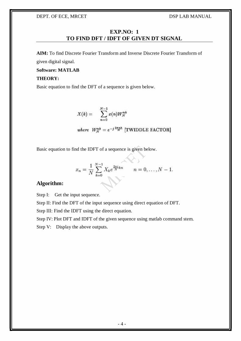
THEORY:
Basic equation to find the DFT of a sequence is given below.
Basic equation to find the IDFT of a sequence is given below.
Algorithm:
Step I: Get the input sequence.
Step II: Find the DFT of the input sequence using direct equation of DFT.
Step III: Find the IDFT using the direct equation.
Step IV: Plot DFT and IDFT of the given sequence using matlab command stem.
Step V: Display the above outputs.
- 5 -
DEPT. OF ECE, MRCET DSP LAB MANUAL
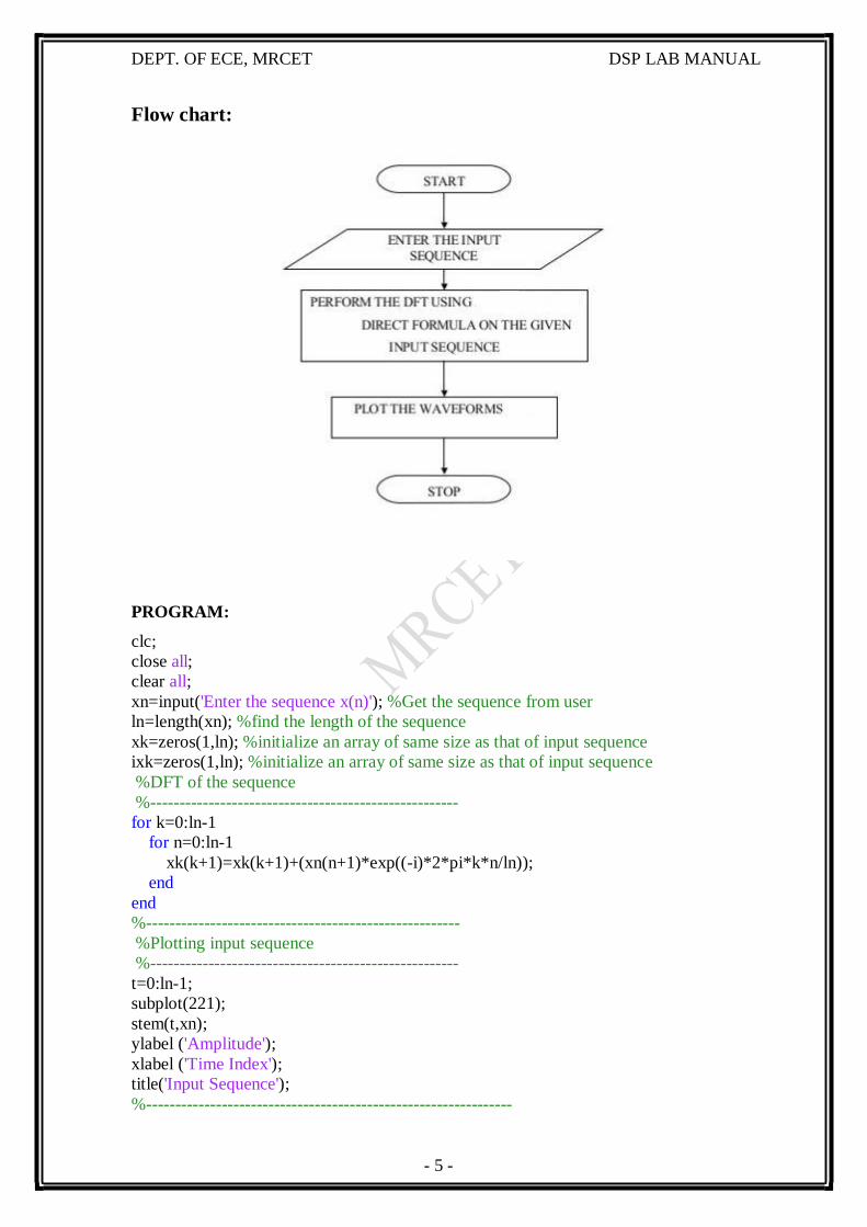
Flow chart:
PROGRAM:
clc;
close all;
clear all;
xn=input('Enter the sequence x(n)'); %Get the sequence from user
ln=length(xn); %find the length of the sequence
xk=zeros(1,ln); %initialize an array of same size as that of input sequence
ixk=zeros(1,ln); %initialize an array of same size as that of input sequence
%DFT of the sequence
%-----------------------------------------------------
for k=0:ln-1
for n=0:ln-1
xk(k+1)=xk(k+1)+(xn(n+1)*exp((-i)*2*pi*k*n/ln));
end
end
%------------------------------------------------------
%Plotting input sequence
%-----------------------------------------------------
t=0:ln-1;
subplot(221);
stem(t,xn);
ylabel ('Amplitude');
xlabel ('Time Index');
title('Input Sequence');
%---------------------------------------------------------------
- 6 -
DEPT. OF ECE, MRCET DSP LAB MANUAL
magnitude=abs(xk); % Find the magnitudes of individual DFT points
% plot the magnitude response
%------------------------------------------------------------
t=0:ln-1;
subplot(222);
stem(t,magnitude);
ylabel ('Amplitude');
xlabel ('K');
title('Magnitude Response');
%------------------------------------------------------------
phase=angle(xk); % Find the phases of individual DFT points % plot the magnitude
sequence
%------------------------------------------------------------
t=0:ln-1;
subplot(223);
stem(t,phase);
ylabel ('Phase');
xlabel ('K');
title ('Phase Response');
%------------------------------------------------------------
%IDFT of the sequence
%------------------------------------------------------------
for n=0:ln-1
for k=0:ln-1
ixk(n+1)=ixk(n+1)+(xk(k+1)*exp(i*2*pi*k*n/ln));
end
end
ixk=ixk./ln;
%------------------------------------------------------------
%code block to plot the input sequence
%------------------------------------------------------------
t=0:ln-1;
subplot(224);
stem(t,ixk);
ylabel ('Amplitude');
xlabel ('Time Index');
title ('IDFT sequence');
%------------------------------------------------------
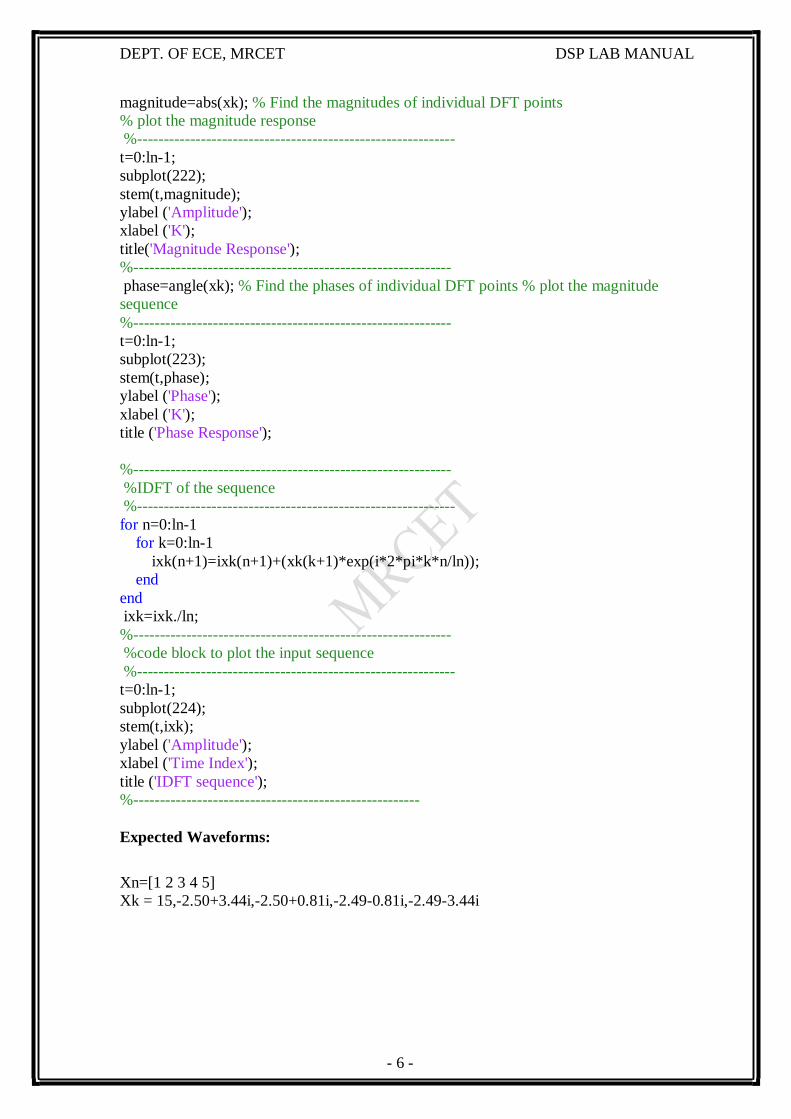
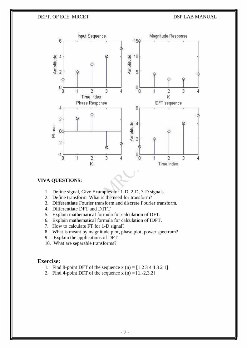
Expected Waveforms:
Xn=[1 2 3 4 5]
Xk = 15,-2.50+3.44i,-2.50+0.81i,-2.49-0.81i,-2.49-3.44i
- 7 -
DEPT. OF ECE, MRCET DSP LAB MANUAL
VIVA QUESTIONS:
1. Define signal, Give Examples for 1-D, 2-D, 3-D signals.
2. Define transform. What is the need for transform? 3. Differentiate Fourier transform and discrete Fourier transform.
4. Differentiate DFT and DTFT
5. Explain mathematical formula for calculation of DFT.
6. Explain mathematical formula for calculation of IDFT.
7. How to calculate FT for 1-D signal?
8. What is meant by magnitude plot, phase plot, power spectrum?
9. Explain the applications of DFT.
10. What are separable transforms?
Exercise: 1. Find 8-point DFT of the sequence x (n) = [1 2 3 4 4 3 2 1] 2. Find 4-point DFT of the sequence x (n) = [1,-2,3,2]

- 8 -
DEPT. OF ECE, MRCET DSP LAB MANUAL
OBSERVATIONS
Output Waveforms:
- 9 -
DEPT. OF ECE, MRCET DSP LAB MANUAL
EXP.NO: 2
LINEAR CONVOLUTION OF TWO SEQUENCES
AIM: To obtain Linear Convolution of two finite length sequences
Software: MATLAB
THEORY:
Convolution is a mathematical operation used to express the relation between
input and output of an LTI system. It relates input, output and impulse response of an
LTI system as
y(n)=x(n)∗h(n)
Where y (n) = output of LTI
x (n) = input of LTI
h (n) = impulse response of LTI
Discrete Convolution
y(n)=x(n)∗h(n)
=
By using convolution we can find zero state response of the system.
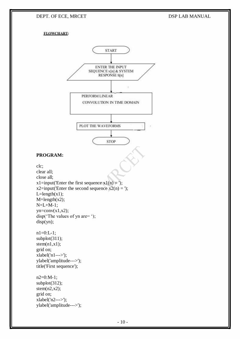
Algorithm:
Step I: Give input sequence x[n].
Step II: Give impulse response sequence h(n)
Step III: Find the convolution y[n] using the matlab command conv.
Step IV: Plot x[n],h[n],y[n].
- 10 -
DEPT. OF ECE, MRCET DSP LAB MANUAL
PROGRAM:
clc;
clear all;
close all;
x1=input('Enter the first sequence x1(n) = ');
x2=input('Enter the second sequence x2(n) = ');
L=length(x1);
M=length(x2);
N=L+M-1;
yn=conv(x1,x2);
disp(‘The values of yn are= ‘);
disp(yn);
n1=0:L-1;
subplot(311);
stem(n1,x1);
grid on;
xlabel('n1--->');
ylabel('amplitude--->');
title('First sequence');
n2=0:M-1;
subplot(312);
stem(n2,x2);
grid on;
xlabel('n2--->');
ylabel('amplitude--->');
- 11 -
DEPT. OF ECE, MRCET DSP LAB MANUAL
title('Second sequence');
n3=0:N-1;
subplot(313); stem(n3,yn);
grid on;
xlabel('n3--->');
ylabel('amplitude--->');
title('Convolved output');
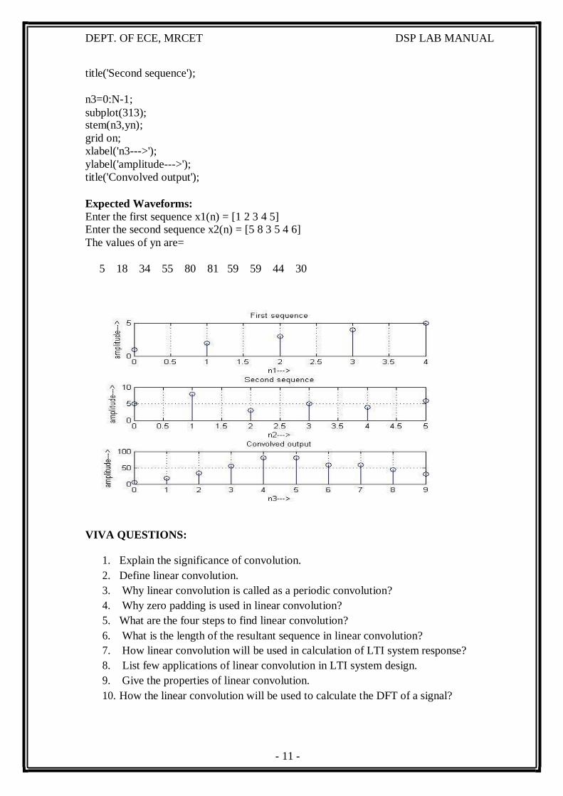
Expected Waveforms:
Enter the first sequence x1(n) = [1 2 3 4 5] Enter the second sequence x2(n) = [5 8 3 5 4 6]
The values of yn are=
5 18 34 55 80 81 59 59 44 30
VIVA QUESTIONS:
1. Explain the significance of convolution.
2. Define linear convolution.
3. Why linear convolution is called as a periodic convolution?
4. Why zero padding is used in linear convolution?
5. What are the four steps to find linear convolution?
6. What is the length of the resultant sequence in linear convolution?
7. How linear convolution will be used in calculation of LTI system response?
8. List few applications of linear convolution in LTI system design.
9. Give the properties of linear convolution.
10. How the linear convolution will be used to calculate the DFT of a signal?
- 12 -
DEPT. OF ECE, MRCET DSP LAB MANUAL
Exercise:
1. Find the linear convolution of x(n)=[7 5 4 0] and h(n)=[0 3 6 2 9]
2. Find the linear convolution of x(n)=[1 -3 0 5 6] and h(n)=[2 4 6 -2 -3]

- 13 -
DEPT. OF ECE, MRCET DSP LAB MANUAL
OBSERVATIONS
Output Waveforms:
- 14 -
DEPT. OF ECE, MRCET DSP LAB MANUAL
EXP.NO: 3
AUTO CORRELATION
AIM: To compute auto correlation between two sequences
SOFTWARE: MATLAB
THEORY:
Auto Correlation Function
Auto correlation function is a measure of similarity between a signal & its time
delayed version. It is represented with R(k).
The auto correlation function of x(n) is given by
R11(k)=R(k)=
Algorithm:
Step I : Give input sequence x[n].
Step II : Give impulse response sequence h (n)
Step III: Find auto correlation using the matlab command xcorr.
Step IV: Plot x[n], h[n], z[n].
Step V: Display the results
- 15 -
DEPT. OF ECE, MRCET DSP LAB MANUAL
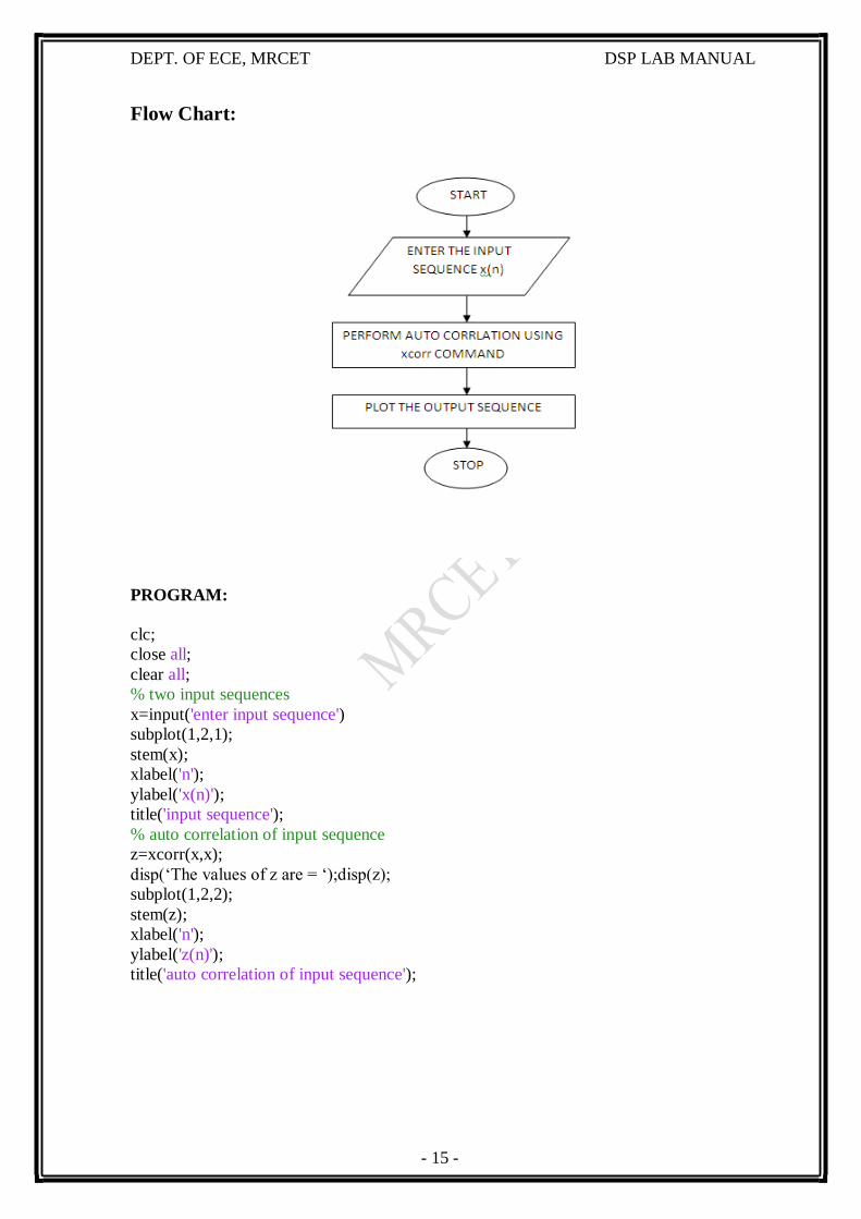
Flow Chart:
PROGRAM:
clc;
close all;
clear all;
% two input sequences
x=input('enter input sequence')
subplot(1,2,1);
stem(x);
xlabel('n');
ylabel('x(n)');
title('input sequence');
% auto correlation of input sequence
z=xcorr(x,x);
disp(‘The values of z are = ‘);disp(z);
subplot(1,2,2);
stem(z);
xlabel('n');
ylabel('z(n)');
title('auto correlation of input sequence');
- 16 -
DEPT. OF ECE, MRCET DSP LAB MANUAL
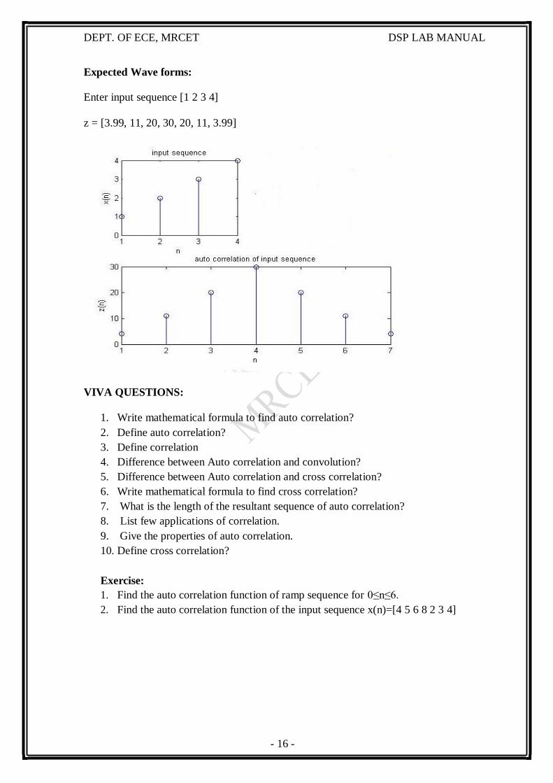
Expected Wave forms:
Enter input sequence [1 2 3 4]
z = [3.99, 11, 20, 30, 20, 11, 3.99]
VIVA QUESTIONS:
1. Write mathematical formula to find auto correlation?
2. Define auto correlation?
3. Define correlation
4. Difference between Auto correlation and convolution?
5. Difference between Auto correlation and cross correlation?
6. Write mathematical formula to find cross correlation?
7. What is the length of the resultant sequence of auto correlation?
8. List few applications of correlation.
9. Give the properties of auto correlation.
10. Define cross correlation?
Exercise:
1. Find the auto correlation function of ramp sequence for 0≤n≤6.
2. Find the auto correlation function of the input sequence x(n)=[4 5 6 8 2 3 4]
- 17 -
DEPT. OF ECE, MRCET DSP LAB MANUAL
OBSERVATIONS
Output Waveforms:
- 18 -
DEPT. OF ECE, MRCET DSP LAB MANUAL
EXP.NO: 4 TO FIND FREQUENCY RESPONSE OF A GIVEN SYSTEM GIVEN
IN (TRANSFER FUNCTION/ DIFFERENTIAL EQUATION FORM)
AIM: To find frequency response of a given system in differential equation form.
Software: MATLAB
THEORY:
Systems respond differently to inputs of different frequencies. Some systems may
amplify components of certain frequencies, and attenuate components of other
frequencies. The way that the system output is related to the system input for different
frequencies is called the frequency response of the system.
Since the frequency response is a complex function, we can convert it to polar
notation in the complex plane. This will give us a magnitude and an angle. We call the
angle the phase.
The phase response, or its derivative the group delay, tells us how the system delays the
input signal as a function of frequency.
Given Difference equation is
Algorithm:
Step I : Give numerator coefficients of the given transfer function or difference
equation.
Step II : Give denominator coefficients of the given transfer function or difference
equation
Step III : Pass these coefficients to matlab command freqz to find frequency response.
Step IV : Find magnitude and phase response using matlab commands abs and angle.
Step V : Plot magnitude and phase response.
Amplitude Response:
For each frequency, the magnitude represents the system's tendency to amplify or
attenuate the input signal.
Phase Response:
The phase represents the system's tendency to modify the phase of the input sinusoids.
- 19 -
DEPT. OF ECE, MRCET DSP LAB MANUAL
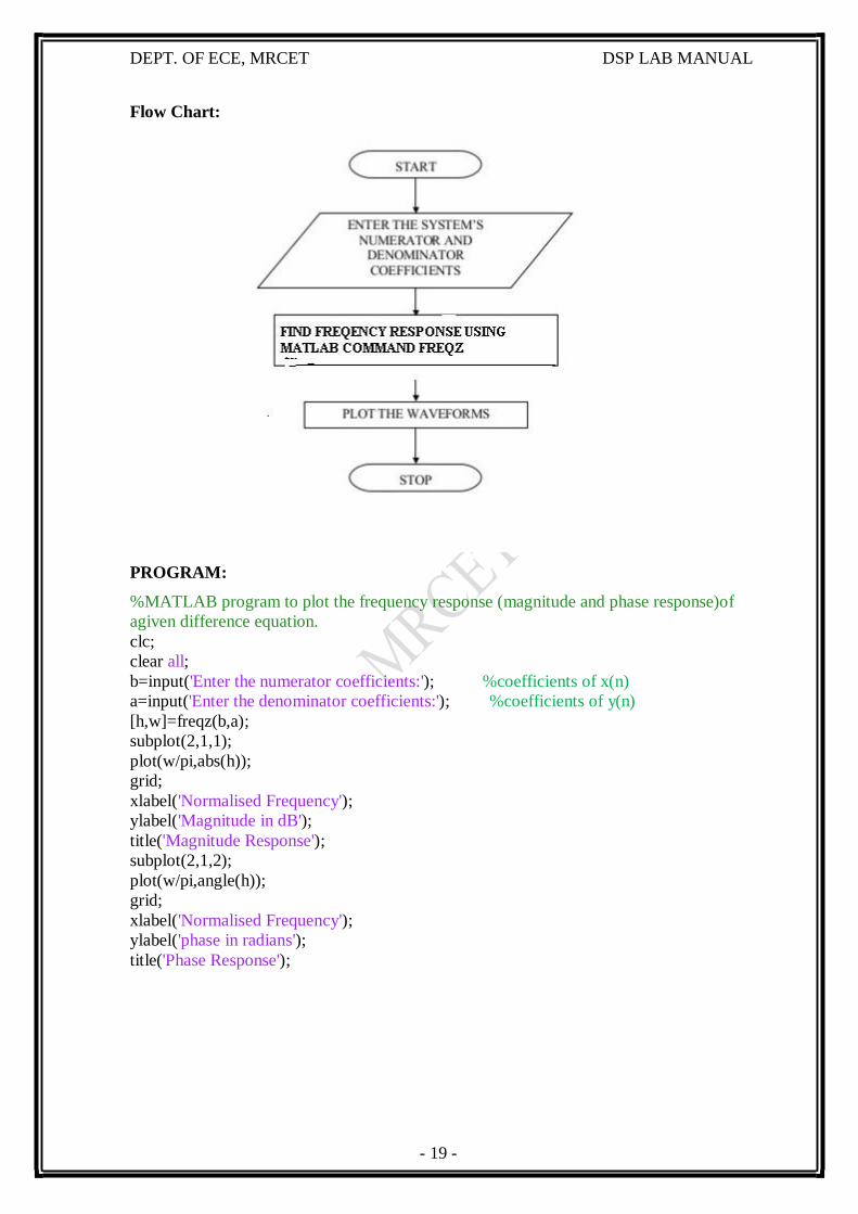
Flow Chart:
PROGRAM:
%MATLAB program to plot the frequency response (magnitude and phase response)of
agiven difference equation.
clc;
clear all;
b=input('Enter the numerator coefficients:'); %coefficients of x(n)
a=input('Enter the denominator coefficients:'); %coefficients of y(n)
[h,w]=freqz(b,a);
subplot(2,1,1);
plot(w/pi,abs(h));
grid;
xlabel('Normalised Frequency');
ylabel('Magnitude in dB');
title('Magnitude Response');
subplot(2,1,2);
plot(w/pi,angle(h));
grid;
xlabel('Normalised Frequency');
ylabel('phase in radians');
title('Phase Response');
- 20 -
VIVA QUESTIONS:
DEPT. OF ECE, MRCET DSP LAB MANUAL
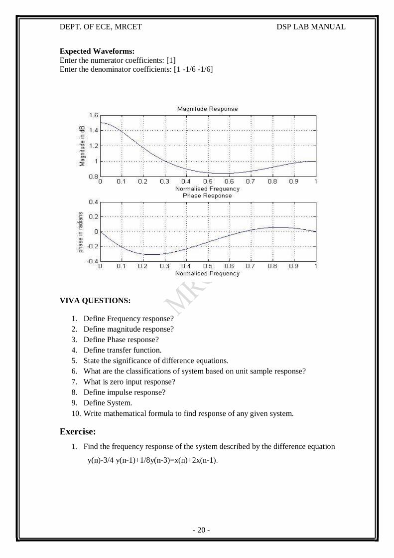
Expected Waveforms:
Enter the numerator coefficients: [1] Enter the denominator coefficients: [1 -1/6 -1/6]
1. Define Frequency response?
2. Define magnitude response?
3. Define Phase response?
4. Define transfer function.
5. State the significance of difference equations.
6. What are the classifications of system based on unit sample response?
7. What is zero input response?
8. Define impulse response?
9. Define System.
10. Write mathematical formula to find response of any given system.
Exercise:
1. Find the frequency response of the system described by the difference equation
y(n)-3/4 y(n-1)+1/8y(n-3)=x(n)+2x(n-1).

- 21 -
DEPT. OF ECE, MRCET DSP LAB MANUAL
OBSERVATIONS
Output Waveforms:
- 22 -
N 1
DEPT. OF ECE, MRCET DSP LAB MANUAL
EXP.NO: 5
TO FIND THE FFT OF A GIVEN SEQUENCE
AIM: To find the FFT of a given sequence.
Software: MATLAB
THEORY:
DFT of a sequence
X k x[n]e j 2 / N kn
n0
Where N= Length of sequence.
K= Frequency Coefficient.
n = Samples in time domain.
FFT: -Fast Fourier transform.
There are two methods.
1. Decimation in time (DIT ) FFT.
2. Decimation in Frequency (DIF) FFT.
Why we need FFT?
The no of multiplications in DFT = N2.
The no of Additions in DFT = N (N-1).
For FFT.
The no of multiplication = N/2 log 2N.
The no of additions = N log2 N.
Algorithm:
Step I : Give input sequence x[n].
Step II : Find the length of the input sequence using length command.
Step III : Find FFT and IFFT using matlab commands fft and ifft.
Step IV : Plot magnitude and phase response
Step V : Display the results
- 23 -
DEPT. OF ECE, MRCET DSP LAB MANUAL
Flow Chart:
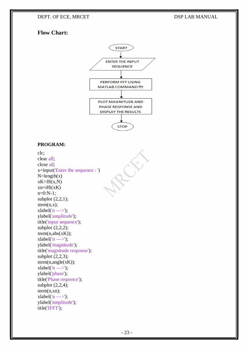
PROGRAM:
clc;
clear all;
close all;
x=input('Enter the sequence : ')
N=length(x)
xK=fft(x,N)
xn=ifft(xK)
n=0:N-1;
subplot (2,2,1);
stem(n,x);
xlabel('n --- >');
ylabel('amplitude');
title('input sequence');
subplot (2,2,2);
stem(n,abs(xK));
xlabel('n --- >');
ylabel('magnitude');
title('magnitude response');
subplot (2,2,3);
stem(n,angle(xK));
xlabel('n --- >');
ylabel('phase');
title('Phase responce');
subplot (2,2,4);
stem(n,xn);
xlabel('n --- >');
ylabel('amplitude');
title('IFFT');
- 24 -
DEPT. OF ECE, MRCET DSP LAB MANUAL
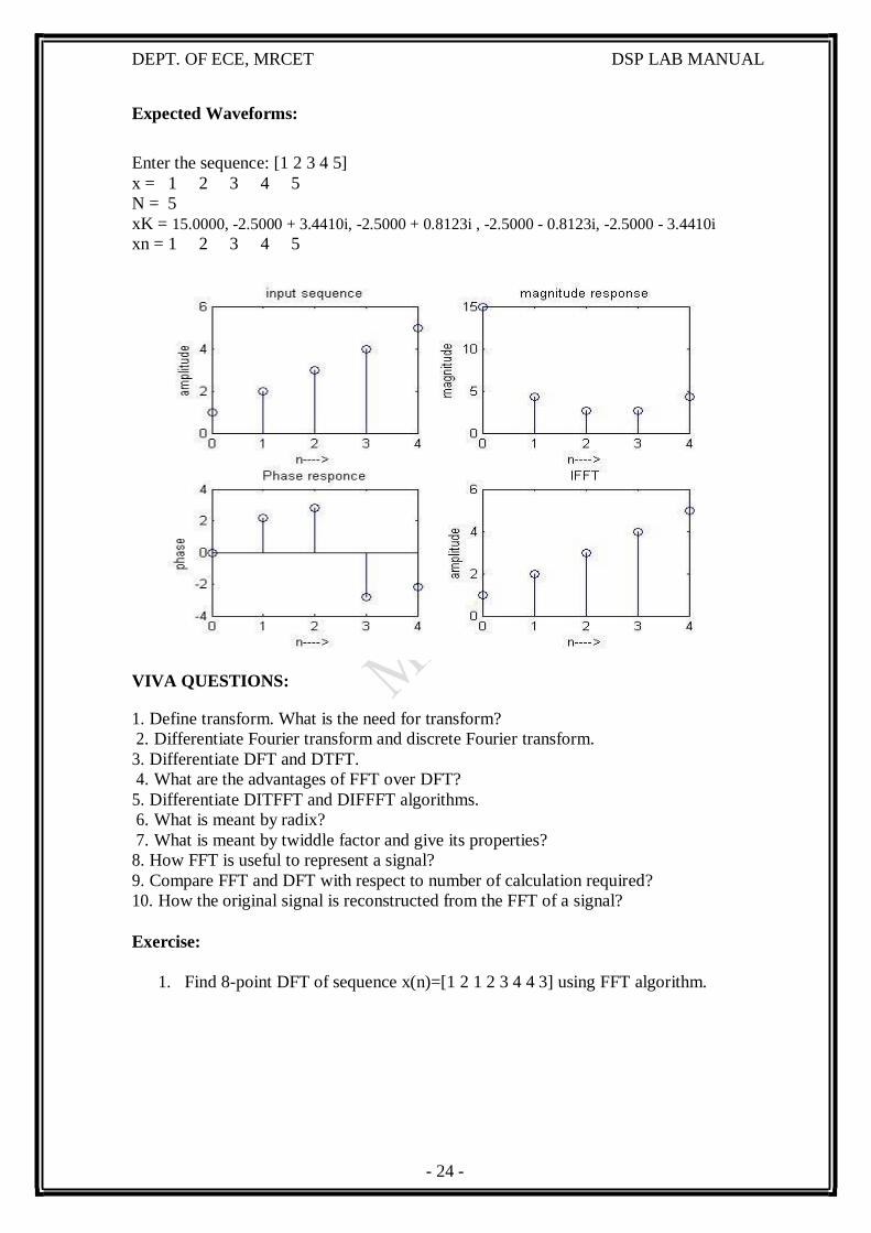
Expected Waveforms:
Enter the sequence: [1 2 3 4 5]
x = 1 2 3 4 5
N = 5
xK = 15.0000, -2.5000 + 3.4410i, -2.5000 + 0.8123i , -2.5000 - 0.8123i, -2.5000 - 3.4410i
xn = 1 2 3 4 5
1. Define transform. What is the need for transform?
2. Differentiate Fourier transform and discrete Fourier transform.
3. Differentiate DFT and DTFT.
4. What are the advantages of FFT over DFT?
5. Differentiate DITFFT and DIFFFT algorithms.
6. What is meant by radix?
7. What is meant by twiddle factor and give its properties?
8. How FFT is useful to represent a signal?
9. Compare FFT and DFT with respect to number of calculation required?
10. How the original signal is reconstructed from the FFT of a signal?
Exercise:
1. Find 8-point DFT of sequence x(n)=[1 2 1 2 3 4 4 3] using FFT algorithm.
VIVA QUESTIONS:

- 25 -
DEPT. OF ECE, MRCET DSP LAB MANUAL
OBSERVATIONS
Output Waveforms:
- 26 -
DEPT. OF ECE, MRCET DSP LAB MANUAL
EXP.NO: 6
DETERMINATION OF POWER SPECTRUM OF A GIVEN SIGNAL
AIM: Determination of Power Spectrum of a given signal.
Software: MATLAB
THEORY:
The power spectrum describes the distribution of signal power over a frequency
spectrum. The most common way of generating a power spectrum is by using a discrete
Fourier transform, but other techniques such as the maximum entropy method can also be
used. The power spectrum can also be defined as the Fourier transform of auto correlation
function.
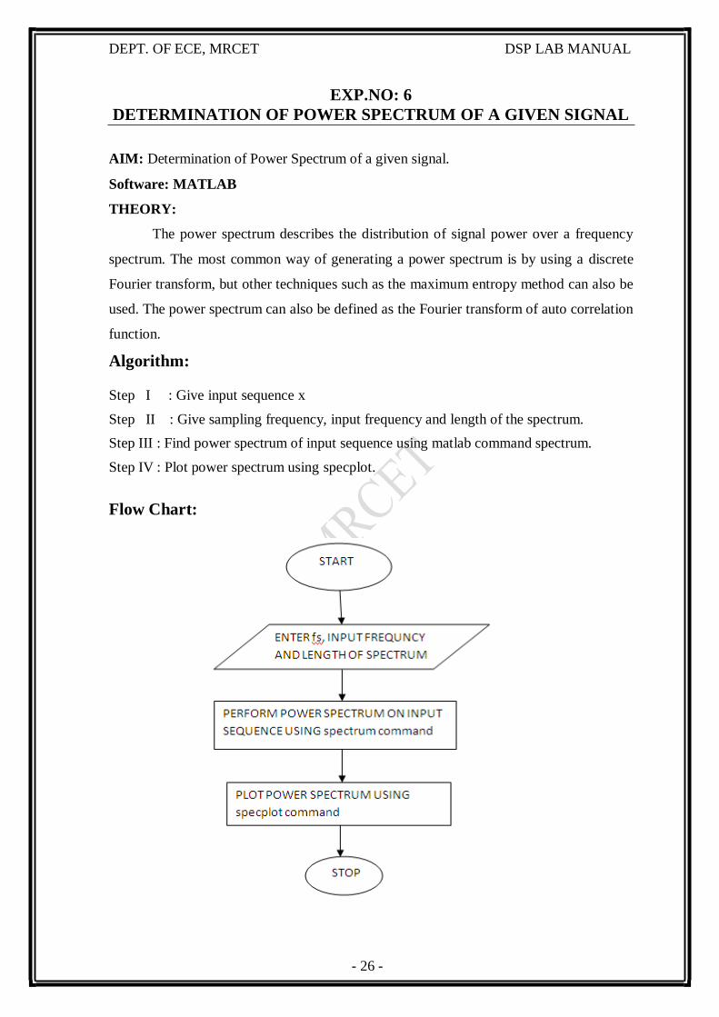
Algorithm:
Step I : Give input sequence x
Step II : Give sampling frequency, input frequency and length of the spectrum.
Step III : Find power spectrum of input sequence using matlab command spectrum.
Step IV : Plot power spectrum using specplot.
Flow Chart:
- 27 -
DEPT. OF ECE, MRCET DSP LAB MANUAL
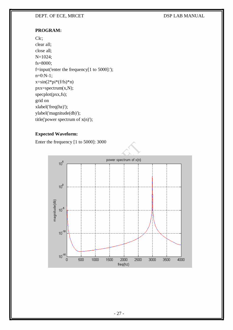
PROGRAM:
Clc;
clear all;
close all;
N=1024;
fs=8000;
f=input('enter the frequency[1 to 5000]:');
n=0:N-1;
x=sin(2*pi*(f/fs)*n)
pxx=spectrum(x,N);
specplot(pxx,fs);
grid on
xlabel('freq(hz)');
ylabel('magnitude(db)');
title('power spectrum of x(n)');
Expected Waveform:
Enter the frequency [1 to 5000]: 3000

- 28 -
DEPT. OF ECE, MRCET DSP LAB MANUAL
VIVA QUESTIONS:
1. Define power signal.
2. Define energy signal.
3. Define power spectral density of a signal.
4. How the energy of a signal can be calculated?
5. Explain difference between energy spectral density and power spectral density.
6. Explain the PSD plot.
7. What is the importance of PSD?
8. What are the applications of PSD?
9. Explain MATLAB function randn(size(n)).
10. What is the need to represent the signal in frequency domain?
Exercise:
1. Find power spectrum of the signal x(n)=cos(2*pi*50*n)

- 29 -
DEPT. OF ECE, MRCET DSP LAB MANUAL
OBSERVATIONS
Output Waveforms:
- 30 -
DEPT. OF ECE, MRCET DSP LAB MANUAL
EXP. NO: 7
IMPLEMENTATION OF LP FIR FILTER
AIM: To implement LP FIR filter for a given sequence.
Software: MATLAB
THEORY:
FIR filters are digital filters with finite impulse response. They are also known
as non-recursive digital filters as they do not have the feedback.
An FIR filter has two important advantages over an IIR design:
Firstly, there is no feedback loop in the structure of an FIR filter. Due to not
having a feedback loop, an FIR filter is inherently stable. Meanwhile, for an IIR
filter, we need to check the stability.
Secondly, an FIR filter can provide a linear-phase response. As a matter of fact,
a linear-phase response is the main advantage of an FIR filter over an IIR
design otherwise, for the same filtering specifications; an IIR filter will lead to
a lower order.
FIR FILTER DESIGN
An FIR filter is designed by finding the coefficients and filter order that meet
certain specifications, which can be in the time-domain (e.g. a matched filter) and/or the
frequency domain (most common). Matched filters perform a cross-correlation between
the input signal and a known pulse-shape. The FIR convolution is a cross-correlation
between the input signal and a time-reversed copy of the impulse-response. Therefore, the
matched-filter's impulse response is "designed" by sampling the known pulse-shape and
using those samples in reverse order as the coefficients of the filter.
When a particular frequency response is desired, several different design methods are
common:
1. Window design method
2. Frequency Sampling method
3. Weighted least squares design
WINDOW DESIGN METHOD
In the window design method, one first designs an ideal IIR filter and then
truncates the infinite impulse response by multiplying it with a finite length window
function. The result is a finite impulse response filter whose frequency response is
modified from that of the IIR filter.
- 31 -
DEPT. OF ECE, MRCET DSP LAB MANUAL
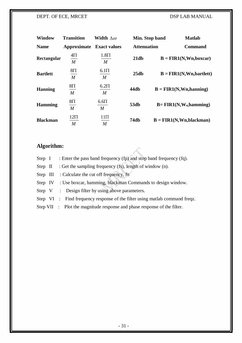
Window Transition Width Min. Stop band Matlab
Name Approximate Exact values Attenuation Command
Rectangular
Bartlett
Hanning
Hamming
Blackman
4
M
8
M
8
M
8
M
12
M
1.8
M
6.1
M
6.2
M
6.6
M
11
M
21db B = FIR1(N,Wn,boxcar)
25db B = FIR1(N,Wn,bartlett)
44db B = FIR1(N,Wn,hanning)
53db B= FIR1(N,Wn,hamming)
74db B = FIR1(N,Wn,blackman)
Algorithm:
Step I : Enter the pass band frequency (fp) and stop band frequency (fq).
Step II : Get the sampling frequency (fs), length of window (n).
Step III : Calculate the cut off frequency, fn
Step IV : Use boxcar, hamming, blackman Commands to design window.
Step V : Design filter by using above parameters.
Step VI : Find frequency response of the filter using matlab command freqz.
Step VII : Plot the magnitude response and phase response of the filter.
- 32 -
DEPT. OF ECE, MRCET DSP LAB MANUAL
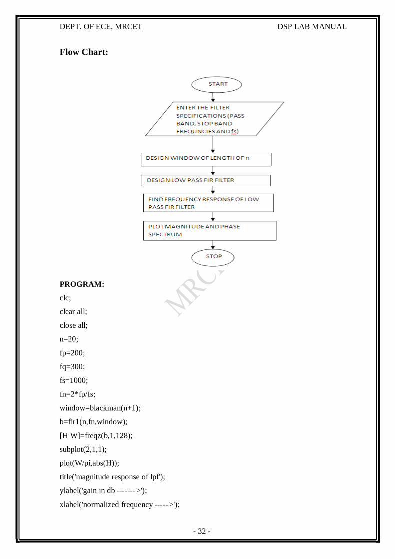
Flow Chart:
PROGRAM:
clc;
clear all;
close all;
n=20;
fp=200;
fq=300;
fs=1000;
fn=2*fp/fs;
window=blackman(n+1);
b=fir1(n,fn,window);
[H W]=freqz(b,1,128);
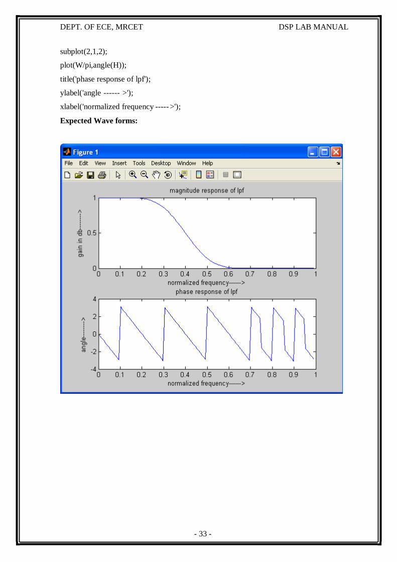
subplot(2,1,1);
plot(W/pi,abs(H));
title('magnitude response of lpf');
ylabel('gain in db ------- >');
xlabel('normalized frequency ----- >');
- 33 -
DEPT. OF ECE, MRCET DSP LAB MANUAL
subplot(2,1,2);
plot(W/pi,angle(H));
title('phase response of lpf');
ylabel('angle ------ >');
xlabel('normalized frequency ----- >');
Expected Wave forms:

- 34 -
DEPT. OF ECE, MRCET DSP LAB MANUAL
VIVA QUESTIONS:
1. Define filter.
2. What are the different types of filters?
3. Why are FIR filters generally preferred over IIR filters in multirate (decimating
and interpolating) systems/
4. Difference between IIR and FIR filters?
5. Differentiate ideal filter and practical filter responses.
6. What is the filter specifications required to design the analog filters?
7. What is meant by frequency response of filter?
8. What is meant by magnitude response?
9. What is meant by phase response?
10. Difference between FIR low pass filter and high pass filter.
Exercise:
1. Design LP FIR filter using Bartlett and hamming window.

- 35 -
DEPT. OF ECE, MRCET DSP LAB MANUAL
OBSERVATIONS
Output Waveforms:
- 36 -
DEPT. OF ECE, MRCET DSP LAB MANUAL
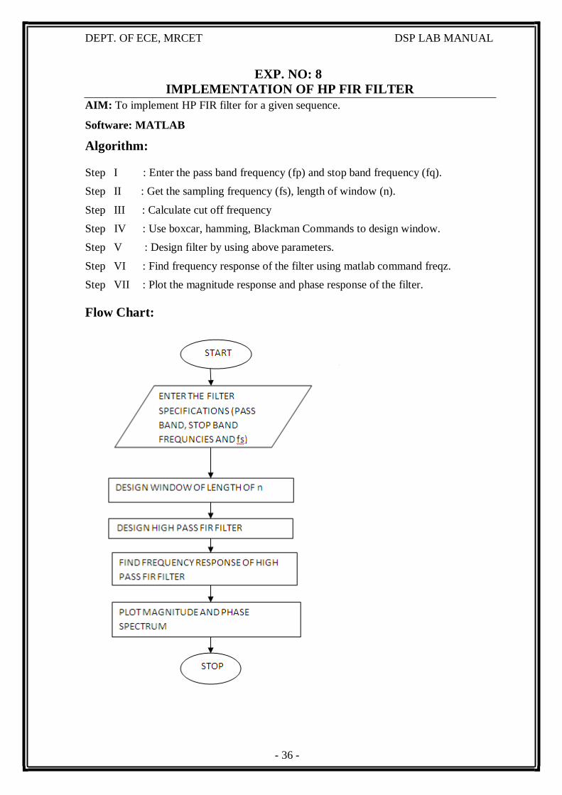
EXP. NO: 8
IMPLEMENTATION OF HP FIR FILTER
AIM: To implement HP FIR filter for a given sequence.
Software: MATLAB
Algorithm:
Step I : Enter the pass band frequency (fp) and stop band frequency (fq).
Step II : Get the sampling frequency (fs), length of window (n).
Step III : Calculate cut off frequency
Step IV : Use boxcar, hamming, Blackman Commands to design window.
Step V : Design filter by using above parameters.
Step VI : Find frequency response of the filter using matlab command freqz.
Step VII : Plot the magnitude response and phase response of the filter.
Flow Chart:
- 37 -
DEPT. OF ECE, MRCET DSP LAB MANUAL
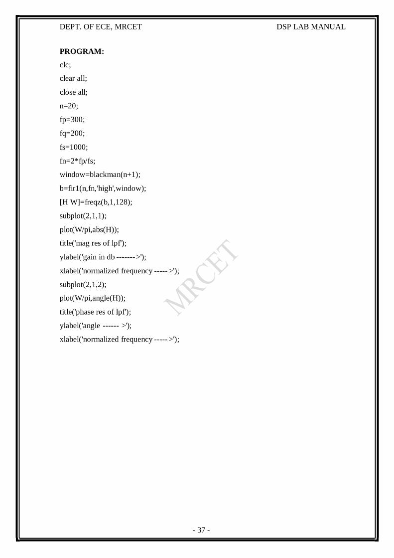
PROGRAM:
clc;
clear all;
close all;
n=20;
fp=300;
fq=200;
fs=1000;
fn=2*fp/fs;
window=blackman(n+1);
b=fir1(n,fn,'high',window);
[H W]=freqz(b,1,128);
subplot(2,1,1);
plot(W/pi,abs(H));
title('mag res of lpf');
ylabel('gain in db ------- >');
xlabel('normalized frequency ----- >');
subplot(2,1,2);
plot(W/pi,angle(H));
title('phase res of lpf');
ylabel('angle ------ >');
xlabel('normalized frequency ----- >');
- 38 -
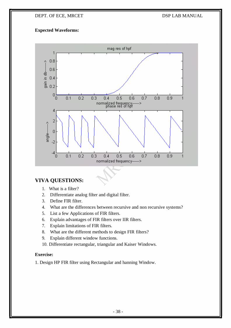
DEPT. OF ECE, MRCET DSP LAB MANUAL
Expected Waveforms:
1. What is a filter?
2. Differentiate analog filter and digital filter.
3. Define FIR filter.
4. What are the differences between recursive and non recursive systems?
5. List a few Applications of FIR filters.
6. Explain advantages of FIR filters over IIR filters.
7. Explain limitations of FIR filters.
8. What are the different methods to design FIR filters?
9. Explain different window functions.
10. Differentiate rectangular, triangular and Kaiser Windows.
Exercise:
1. Design HP FIR filter using Rectangular and hanning Window.
VIVA QUESTIONS:
- 39 -
DEPT. OF ECE, MRCET DSP LAB MANUAL
OBSERVATIONS
Output Waveforms:
- 40 -
DEPT. OF ECE, MRCET DSP LAB MANUAL
EXP. NO: 9
IMPLEMENTATION OF LP IIR FILTER
AIM: To implement LP IIR filter for a given sequence.
Software: MATLAB
THEORY:
IIR filters are digital filters with infinite impulse response. Unlike FIR filters, they
have the feedback (a recursive part of a filter) and are known as recursive digital filters
therefore.
For this reason IIR filters have much better frequency response than FIR filters of
the same order. Unlike FIR filters, their phase characteristic is not linear which can cause
a problem to the systems which need phase linearity. For this reason, it is not preferable
to use IIR filters in digital signal processing when the phase is of the essence. Otherwise,
when the linear phase characteristic is not important, the use of IIR filters is an excellent
IIR FILTER DESIGN
For the given specifications to Design a digital IIR filter, first we need to design
analog filter (Butterworth or chebyshev). The resultant analog filter is transformed to
digital filter by using either “Bilinear transformation or Impulse Invariant
transformation”.
solution.
There is one problem known as a potential instability that is typical of IIR filters only.
FIR filters do not have such a problem as they do not have the feedback. For this reason,
it is always necessary to check after the design process whether the resulting IIR filter is
stable or not.
- 41 -
DEPT. OF ECE, MRCET DSP LAB MANUAL
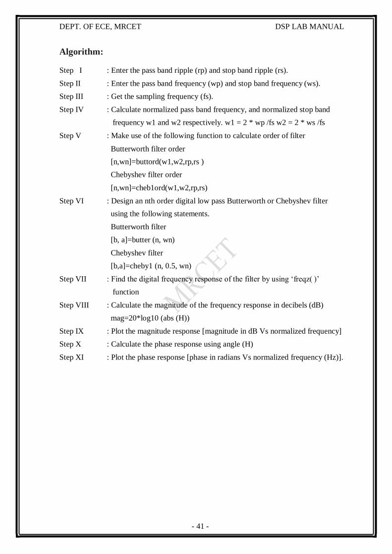
Algorithm:
Step I : Enter the pass band ripple (rp) and stop band ripple (rs).
Step II : Enter the pass band frequency (wp) and stop band frequency (ws).
Step III : Get the sampling frequency (fs).
Step IV : Calculate normalized pass band frequency, and normalized stop band
frequency w1 and w2 respectively. w1 = 2 * wp /fs w2 = 2 * ws /fs
Step V : Make use of the following function to calculate order of filter
Butterworth filter order
[n,wn]=buttord(w1,w2,rp,rs )
Chebyshev filter order
[n,wn]=cheb1ord(w1,w2,rp,rs)
Step VI : Design an nth order digital low pass Butterworth or Chebyshev filter
using the following statements.
Butterworth filter
[b, a]=butter (n, wn)
Chebyshev filter
[b,a]=cheby1 (n, 0.5, wn)
Step VII : Find the digital frequency response of the filter by using ‘freqz( )’
function
Step VIII : Calculate the magnitude of the frequency response in decibels (dB)
mag=20*log10 (abs (H))
Step IX : Plot the magnitude response [magnitude in dB Vs normalized frequency]
Step X : Calculate the phase response using angle (H)
Step XI : Plot the phase response [phase in radians Vs normalized frequency (Hz)].
- 42 -
DEPT. OF ECE, MRCET DSP LAB MANUAL
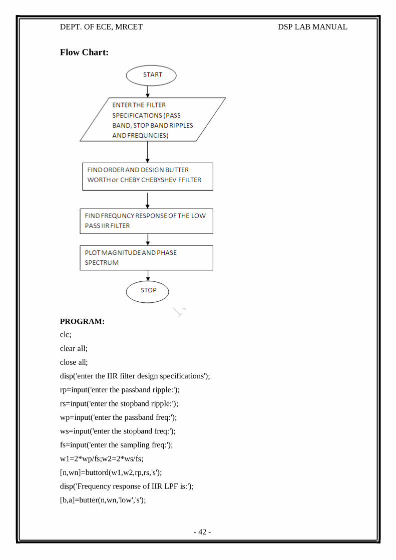
Flow Chart:
PROGRAM:
clc;
clear all;
close all;
disp('enter the IIR filter design specifications');
rp=input('enter the passband ripple:');
rs=input('enter the stopband ripple:');
wp=input('enter the passband freq:');
ws=input('enter the stopband freq:');
fs=input('enter the sampling freq:');
w1=2*wp/fs;w2=2*ws/fs;
[n,wn]=buttord(w1,w2,rp,rs,'s');
disp('Frequency response of IIR LPF is:');
[b,a]=butter(n,wn,'low','s');
- 43 -
DEPT. OF ECE, MRCET DSP LAB MANUAL
w=0:.01:pi;
[h,om]=freqs(b,a,w);
m=20*log10(abs(h));
an=angle(h);
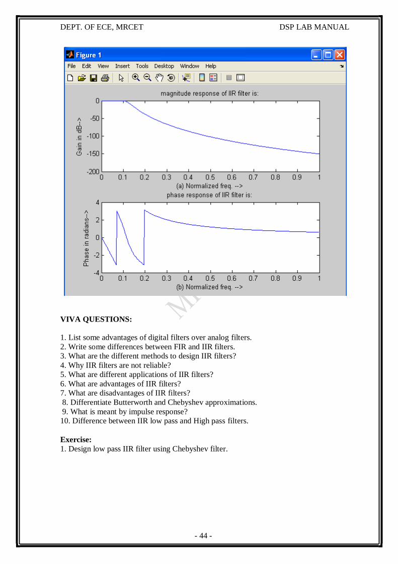
figure,subplot(2,1,1);plot(om/pi,m);
title('magnitude response of IIR filter is:');
xlabel('(a) Normalized freq. -->');
ylabel('Gain in dB-->');
subplot(2,1,2);plot(om/pi,an);
title('phase response of IIR filter is:');
xlabel('(b) Normalized freq. -->');
ylabel('Phase in radians-->');
Expected waveforms:
enter the IIR filter design specifications
enter the passband ripple:15
enter the stopband ripple:60
enter the passband freq:1500
enter the stopband freq:3000
enter the sampling freq:7000
- 44 -
DEPT. OF ECE, MRCET DSP LAB MANUAL
VIVA QUESTIONS:
1. List some advantages of digital filters over analog filters.
2. Write some differences between FIR and IIR filters.
3. What are the different methods to design IIR filters?
4. Why IIR filters are not reliable?
5. What are different applications of IIR filters?
6. What are advantages of IIR filters?
7. What are disadvantages of IIR filters?
8. Differentiate Butterworth and Chebyshev approximations.
9. What is meant by impulse response?
10. Difference between IIR low pass and High pass filters.
Exercise:
1. Design low pass IIR filter using Chebyshev filter.

- 45 -
DEPT. OF ECE, MRCET DSP LAB MANUAL
OBSERVATIONS
Output Waveforms:
- 46 -
DEPT. OF ECE, MRCET DSP LAB MANUAL
EXP. NO: 10
IMPLEMENTATION OF HP IIR FILTER
AIM: To implement HP IIR filter for a given sequence.
Software: MATLAB
Algorithm:
Step I : Enter the pass band ripple (rp) and stop band ripple (rs).
Step II : the pass band frequency (wp) and stop band frequency (ws).
Step III : Get the sampling frequency (fs).
Step IV : Calculate normalized pass band frequency, and normalized stop band
frequency w1 and w2 respectively. w1 = 2 * wp /fs w2 = 2 * ws /fs
Step V : Make use of the following function to calculate order of filter
Butterworth filter order
[n,wn]=buttord(w1,w2,rp,rs )
Chebyshev filter order
[n,wn]=cheb1ord(w1,w2,rp,rs)
Step VI : Design an nth order digital high pass Butterworth or Chebyshev filter
using the following statement.
Butterworth filter
[b,a]=butter (n, wn,’high’)
Chebyshev filter
[b,a]=cheby1 (n, 0.5, wn,'high')
Step VII : Find the digital frequency response of the filter by using ‘freqz( )’
function
Step VIII : Calculate the magnitude of the frequency response in decibels (dB)
mag=20*log10 (abs (H))
Step IX : Plot the magnitude response [magnitude in dB Vs normalized frequency]
Step X : Calculate the phase response using angle (H)
Step XI : Plot the phase response [phase in radians Vs normalized frequency (Hz)].
- 47 -
DEPT. OF ECE, MRCET DSP LAB MANUAL
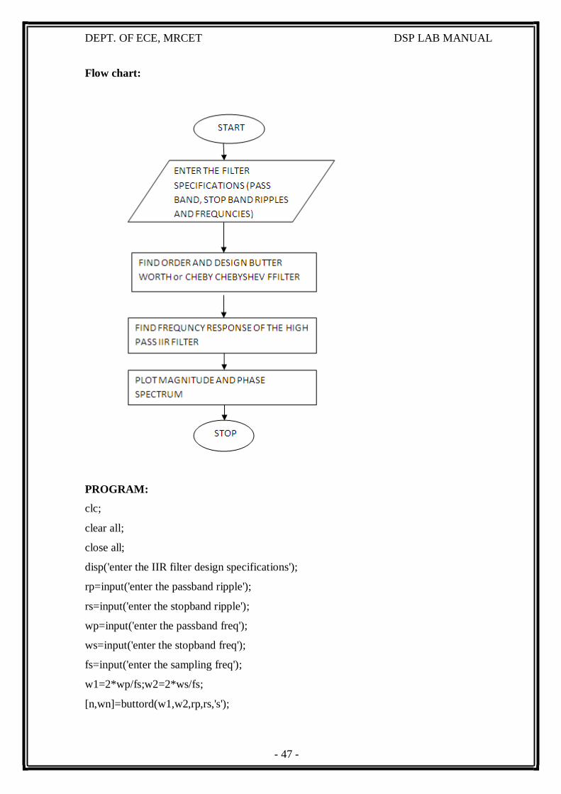
Flow chart:
PROGRAM:
clc;
clear all;
close all;
disp('enter the IIR filter design specifications');
rp=input('enter the passband ripple');
rs=input('enter the stopband ripple');
wp=input('enter the passband freq');
ws=input('enter the stopband freq');
fs=input('enter the sampling freq');
w1=2*wp/fs;w2=2*ws/fs;
[n,wn]=buttord(w1,w2,rp,rs,'s');
- 48 -
DEPT. OF ECE, MRCET DSP LAB MANUAL
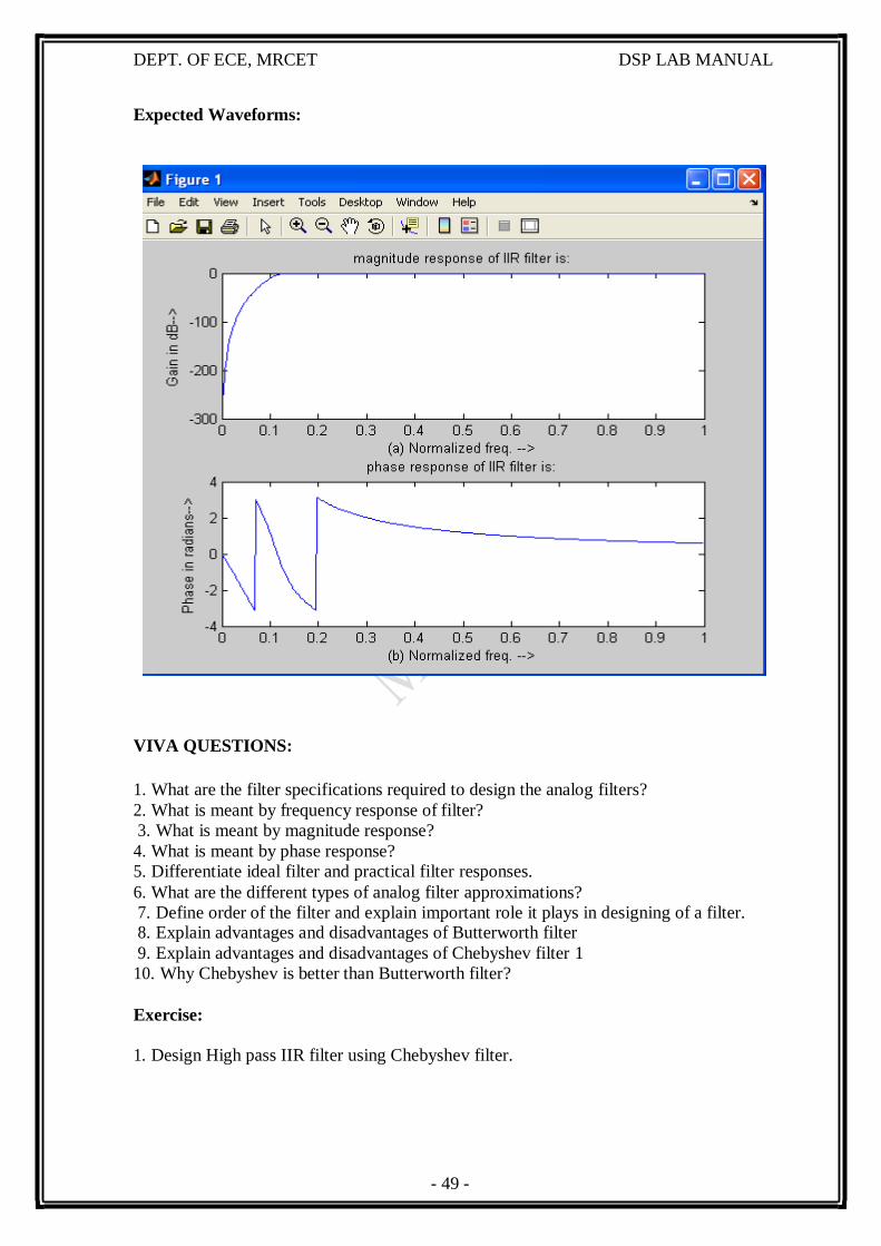
disp('Frequency response of IIR HPF is:');
[b,a]=butter(n,wn,'high','s');
w=0:.01:pi;
[h,om]=freqs(b,a,w);
m=20*log10(abs(h));
an=angle(h);
figure,subplot(2,1,1);plot(om/pi,m);
title('magnitude response of IIR filter is:');
xlabel('(a) Normalized freq. -->');
ylabel('Gain in dB-->');
subplot(2,1,2);plot(om/pi,an);
title('phase response of IIR filter is:');
xlabel('(b) Normalized freq. -->');
ylabel('Phase in radians-->');
INPUT:
enter the IIR filter design specifications
enter the passband ripple15
enter the stopband ripple60
enter the passband freq1500
enter the stopband freq3000
enter the sampling freq7000
- 49 -
DEPT. OF ECE, MRCET DSP LAB MANUAL
Expected Waveforms:
VIVA QUESTIONS:
1. What are the filter specifications required to design the analog filters?
2. What is meant by frequency response of filter?
3. What is meant by magnitude response?
4. What is meant by phase response?
5. Differentiate ideal filter and practical filter responses.
6. What are the different types of analog filter approximations?
7. Define order of the filter and explain important role it plays in designing of a filter. 8. Explain advantages and disadvantages of Butterworth filter
9. Explain advantages and disadvantages of Chebyshev filter 1
10. Why Chebyshev is better than Butterworth filter?
Exercise:
1. Design High pass IIR filter using Chebyshev filter.

- 50 -
DEPT. OF ECE, MRCET DSP LAB MANUAL
OBSERVATIONS
Output Waveforms:
- 51 -
DEPT. OF ECE, MRCET DSP LAB MANUAL
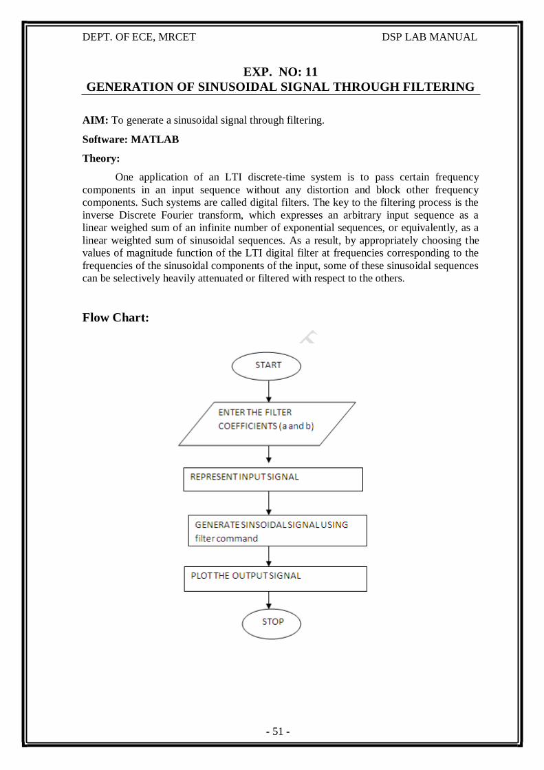
EXP. NO: 11
GENERATION OF SINUSOIDAL SIGNAL THROUGH FILTERING
AIM: To generate a sinusoidal signal through filtering.
Software: MATLAB
Theory:
One application of an LTI discrete-time system is to pass certain frequency
components in an input sequence without any distortion and block other frequency
components. Such systems are called digital filters. The key to the filtering process is the
inverse Discrete Fourier transform, which expresses an arbitrary input sequence as a
linear weighed sum of an infinite number of exponential sequences, or equivalently, as a
linear weighted sum of sinusoidal sequences. As a result, by appropriately choosing the
values of magnitude function of the LTI digital filter at frequencies corresponding to the
frequencies of the sinusoidal components of the input, some of these sinusoidal sequences
can be selectively heavily attenuated or filtered with respect to the others.
Flow Chart:
- 52 -
DEPT. OF ECE, MRCET DSP LAB MANUAL
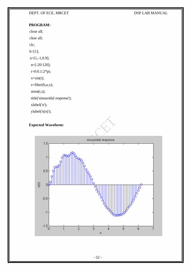
PROGRAM:
close all;
clear all;
clc;
b=[1];
a=[1,-1,0.9];
n=[-20:120];
t=0:0.1:2*pi;
x=sin(t);
s=filter(b,a,x);
stem(t,s);
title('sinusoidal response');
xlabel('n');
ylabel('s(n)');
Expected Waveform:

- 53 -
DEPT. OF ECE, MRCET DSP LAB MANUAL
VIVA QUESTIONS:
1. Define sequence and signal?
2. Differentiate periodic and non-periodic signals?
3. Define period of the signal?
4. Define LTI system.
5. What is filtering?
Exercise:
1. Generate sinusoidal signal using filtering with coefficients a= [1 3 7 8] & b= [0 1].

- 54 -
DEPT. OF ECE, MRCET DSP LAB MANUAL
OBSERVATIONS
Output Waveforms:
- 55 -
DEPT. OF ECE, MRCET DSP LAB MANUAL
EXP. NO: 12
GENERATION OF DTMF SIGNALS
AIM: To generate DTMF Signals using MATLAB Software.
Software: MATLAB
THEORY:
The DTMF stands for “Dual Tone Multi Frequency”, and is a method of
representing digits with tone frequencies, in order to transmit them over an analog
communications network, for example a telephone line. In telephone networks, DTMF
signals are used to encode dial trains and other information.
Dual-tone Multi-Frequency (DTMF) signaling is the basis for voice
communications control and is widely used worldwide in modern telephony to dial
numbers and configure switchboards. It is also used in systems such as in voice mail,
electronic mail and telephone banking.
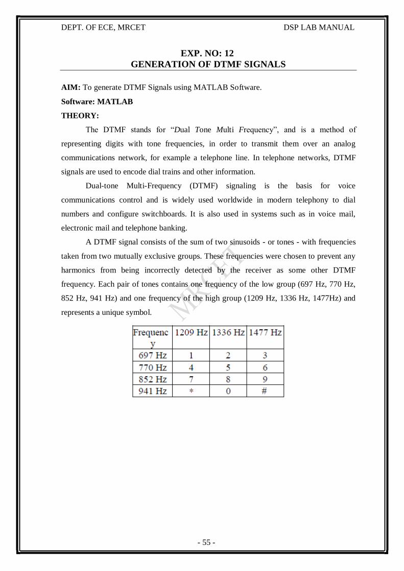
A DTMF signal consists of the sum of two sinusoids - or tones - with frequencies
taken from two mutually exclusive groups. These frequencies were chosen to prevent any
harmonics from being incorrectly detected by the receiver as some other DTMF
frequency. Each pair of tones contains one frequency of the low group (697 Hz, 770 Hz,
852 Hz, 941 Hz) and one frequency of the high group (1209 Hz, 1336 Hz, 1477Hz) and
represents a unique symbol.
- 56 -
DEPT. OF ECE, MRCET DSP LAB MANUAL
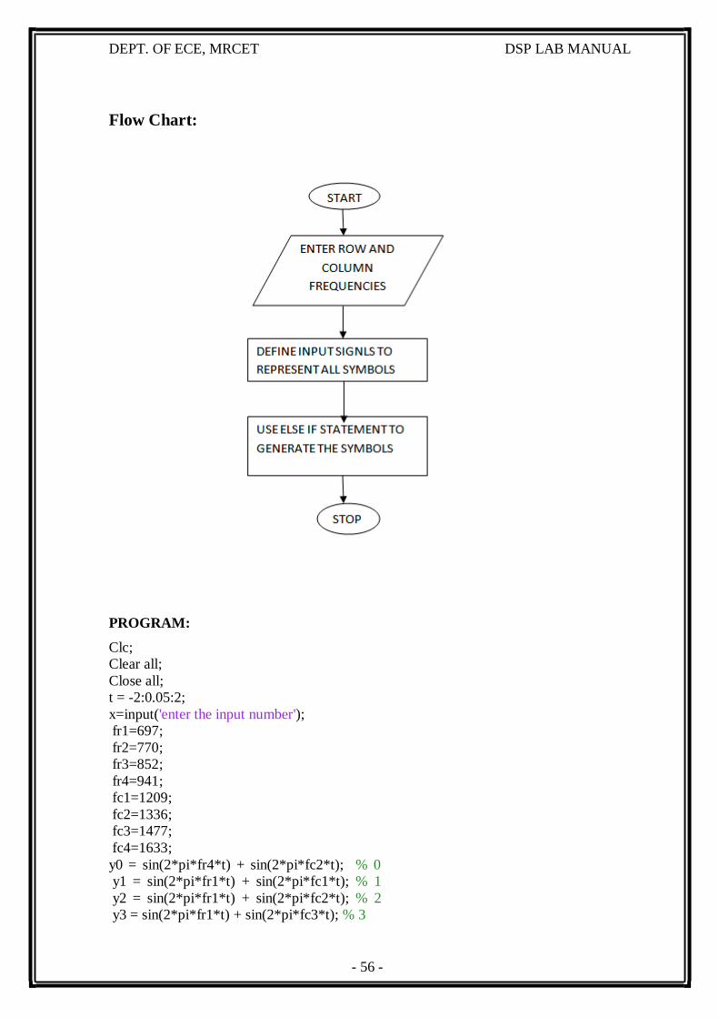
Flow Chart:
PROGRAM:
Clc;
Clear all;
Close all;
t = -2:0.05:2;
x=input('enter the input number');
fr1=697;
fr2=770;
fr3=852;
fr4=941;
fc1=1209;
fc2=1336;
fc3=1477;
fc4=1633;
y0 = sin(2*pi*fr4*t) + sin(2*pi*fc2*t); % 0
y1 = sin(2*pi*fr1*t) + sin(2*pi*fc1*t); % 1
y2 = sin(2*pi*fr1*t) + sin(2*pi*fc2*t); % 2
y3 = sin(2*pi*fr1*t) + sin(2*pi*fc3*t); % 3
- 57 -
DEPT. OF ECE, MRCET DSP LAB MANUAL
y4 = sin(2*pi*fr2*t) + sin(2*pi*fc1*t); % 4
y5 = sin(2*pi*fr2*t) + sin(2*pi*fc2*t); % 5
y6 = sin(2*pi*fr2*t) + sin(2*pi*fc3*t); % 6
y7 = sin(2*pi*fr3*t) + sin(2*pi*fc1*t); % 7
y8 = sin(2*pi*fr3*t) + sin(2*pi*fc2*t); % 8
y9 = sin(2*pi*fr3*t) + sin(2*pi*fc3*t); % 9
y_start = sin(2*pi*fr4*t) + sin(2*pi*fc1*t); % *
y_canc = sin(2*pi*fr4*t) + sin(2*pi*fc3*t); % #
if (x==1)
plot(t,y1)
xlabel('time(t)')
ylabel('amplitude')
elseif (x==2)
plot(t,y2)
xlabel('time(t)')
ylabel('amplitude')
elseif (x==3)
plot(t,y3)
xlabel('time(t)')
ylabel('amplitude')
elseif (x==4)
plot(t,y4)
xlabel('time(t)')
ylabel('amplitude')
elseif (x==5)
plot(t,y5)
xlabel('time(t)')
ylabel('amplitude')
elseif (x==6)
plot(t,y6)
xlabel('time(t)')
ylabel('amplitude')
elseif (x==7)
plot(t,y7)
xlabel('time(t)')
ylabel('amplitude')
elseif (x==8)
plot(t,y8)
xlabel('time(t)')
ylabel('amplitude')
elseif (x==9)
plot(t,y9)
xlabel('time(t)')
ylabel('amplitude')
elseif (x==0)
plot(t,y0)
xlabel('time(t)')
ylabel('amplitude')
elseif (x==11)
plot(t,y_start)
- 58 -
DEPT. OF ECE, MRCET DSP LAB MANUAL
xlabel('time(t)')
ylabel('amplitude')
elseif (x==12)
plot(t,y_canc)
xlabel('time(t)')
ylabel('amplitude')
else
disp('enter the correct input')
end
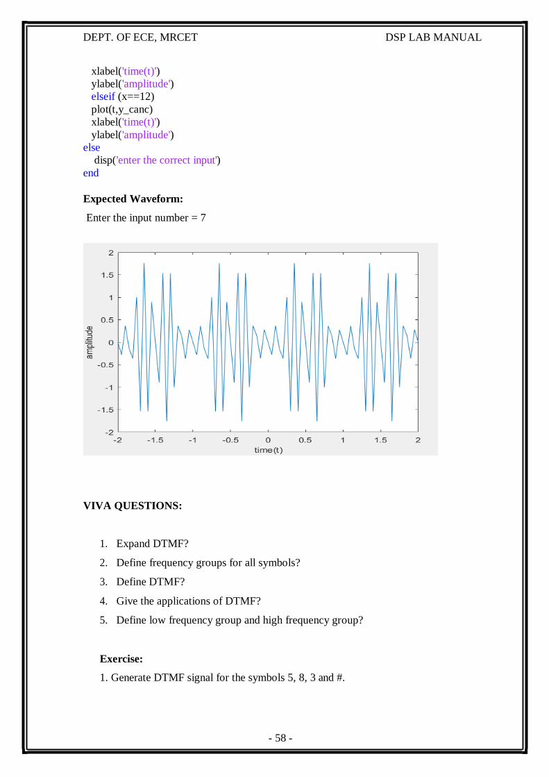
Expected Waveform:
Enter the input number = 7
VIVA QUESTIONS:
1. Expand DTMF?
2. Define frequency groups for all symbols?
3. Define DTMF?
4. Give the applications of DTMF?
5. Define low frequency group and high frequency group?
Exercise:
1. Generate DTMF signal for the symbols 5, 8, 3 and #.

- 59 -
DEPT. OF ECE, MRCET DSP LAB MANUAL
OBSERVATIONS
Output Waveforms:
- 60 -
DEPT. OF ECE, MRCET DSP LAB MANUAL
EXP. NO: 13
IMPLEMENTATION OF DECIMATION PROCESS
AIM: program to verify the decimation of given sequence.
SOFTWARE: MATLAB
THEORY:
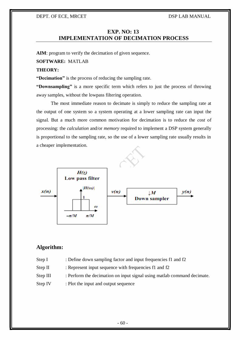
“Decimation” is the process of reducing the sampling rate.
“Downsampling” is a more specific term which refers to just the process of throwing
away samples, without the lowpass filtering operation.
The most immediate reason to decimate is simply to reduce the sampling rate at
the output of one system so a system operating at a lower sampling rate can input the
signal. But a much more common motivation for decimation is to reduce the cost of
processing: the calculation and/or memory required to implement a DSP system generally
is proportional to the sampling rate, so the use of a lower sampling rate usually results in
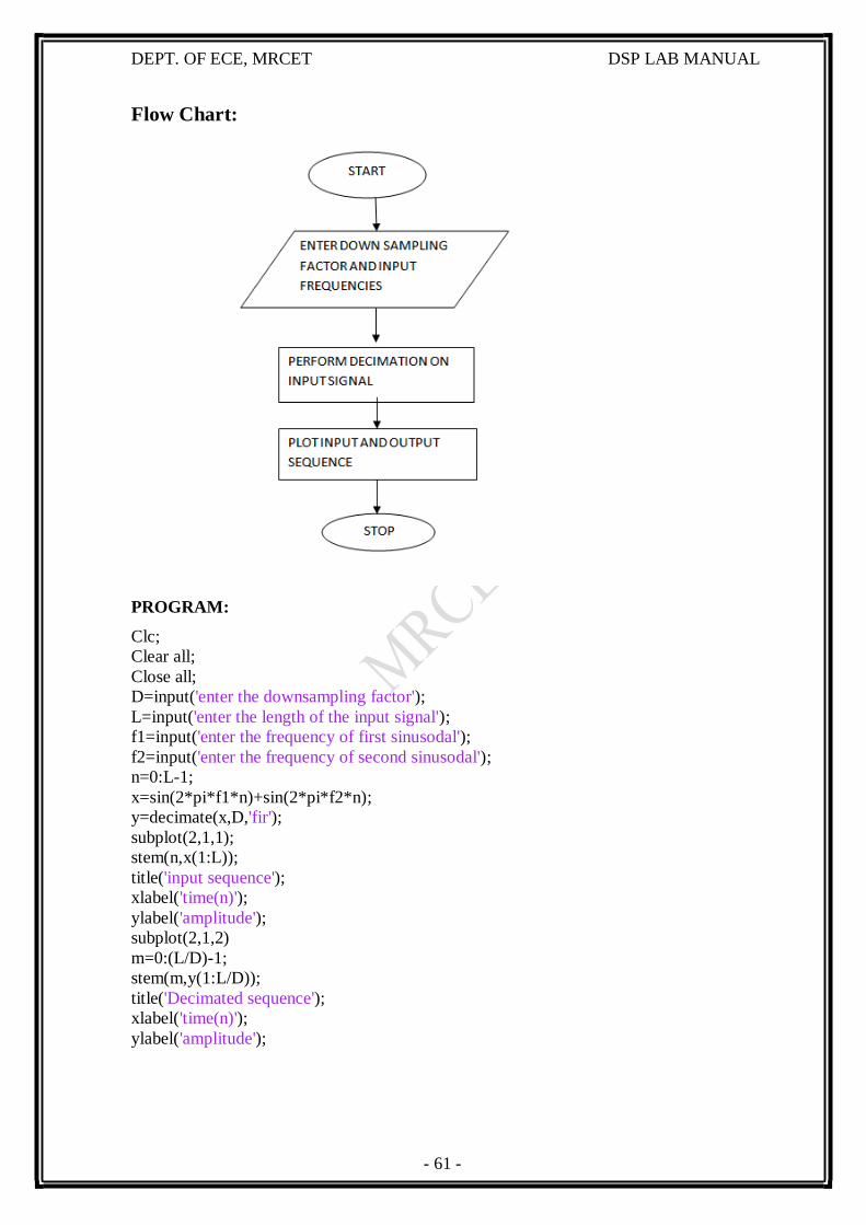
Algorithm:
Step I : Define down sampling factor and input frequencies f1 and f2
Step II : Represent input sequence with frequencies f1 and f2
Step III : Perform the decimation on input signal using matlab command decimate.
Step IV : Plot the input and output sequence
a cheaper implementation.
- 61 -
DEPT. OF ECE, MRCET DSP LAB MANUAL
Flow Chart:
PROGRAM:
Clc;
Clear all;
Close all;
D=input('enter the downsampling factor');
L=input('enter the length of the input signal');
f1=input('enter the frequency of first sinusodal');
f2=input('enter the frequency of second sinusodal');
n=0:L-1;
x=sin(2*pi*f1*n)+sin(2*pi*f2*n);
y=decimate(x,D,'fir');
subplot(2,1,1);
stem(n,x(1:L));
title('input sequence');
xlabel('time(n)');
ylabel('amplitude');
subplot(2,1,2)
m=0:(L/D)-1;
stem(m,y(1:L/D));
title('Decimated sequence');
xlabel('time(n)');
ylabel('amplitude');
- 62 -
DEPT. OF ECE, MRCET DSP LAB MANUAL
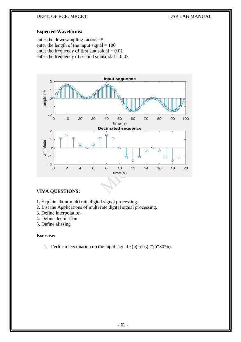
Expected Waveforms:
enter the downsampling factor = 5
enter the length of the input signal = 100
enter the frequency of first sinusoidal = 0.01
enter the frequency of second sinusoidal = 0.03
1. Explain about multi rate digital signal processing.
2. List the Applications of multi rate digital signal processing.
3. Define interpolation.
4. Define decimation.
5. Define aliasing
Exercise:
1. Perform Decimation on the input signal x(n)=cos(2*pi*30*n).
VIVA QUESTIONS:
- 63 -
DEPT. OF ECE, MRCET DSP LAB MANUAL
OBSERVATIONS
Output Waveforms:
- 64 -
DEPT. OF ECE, MRCET DSP LAB MANUAL
EXP. NO: 14
IMPLEMENTATION OF INTERPOLATION PROCESS
AIM: program to verify the decimation of given sequence.
SOFTWARE: MATLAB
THEORY
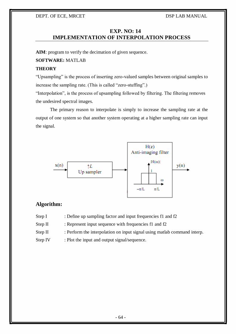
“Upsampling” is the process of inserting zero-valued samples between original samples to
increase the sampling rate. (This is called “zero-stuffing”.)
“Interpolation”, is the process of upsampling followed by filtering. The filtering removes
the undesired spectral images.
The primary reason to interpolate is simply to increase the sampling rate at the
output of one system so that another system operating at a higher sampling rate can input
the signal.
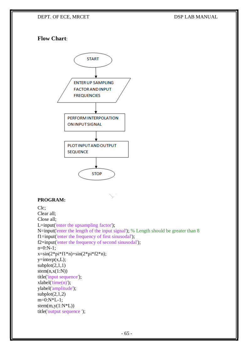
Algorithm:
Step I : Define up sampling factor and input frequencies f1 and f2
Step II : Represent input sequence with frequencies f1 and f2
Step II : Perform the interpolation on input signal using matlab command interp.
Step IV : Plot the input and output signal/sequence.
- 65 -
DEPT. OF ECE, MRCET DSP LAB MANUAL
Flow Chart:
Clc;
Clear all;
Close all;
L=input('enter the upsampling factor'); N=input('enter the length of the input signal'); % Length should be greater than 8
f1=input('enter the frequency of first sinusodal');
f2=input('enter the frequency of second sinusodal');
n=0:N-1;
x=sin(2*pi*f1*n)+sin(2*pi*f2*n);
y=interp(x,L);
subplot(2,1,1)
stem(n,x(1:N))
title('input sequence');
xlabel('time(n)');
ylabel('amplitude');
subplot(2,1,2)
m=0:N*L-1;
stem(m,y(1:N*L))
title('output sequence ');
PROGRAM:
- 66 -
DEPT. OF ECE, MRCET DSP LAB MANUAL
xlabel('time(n)');
ylabel('amplitude');
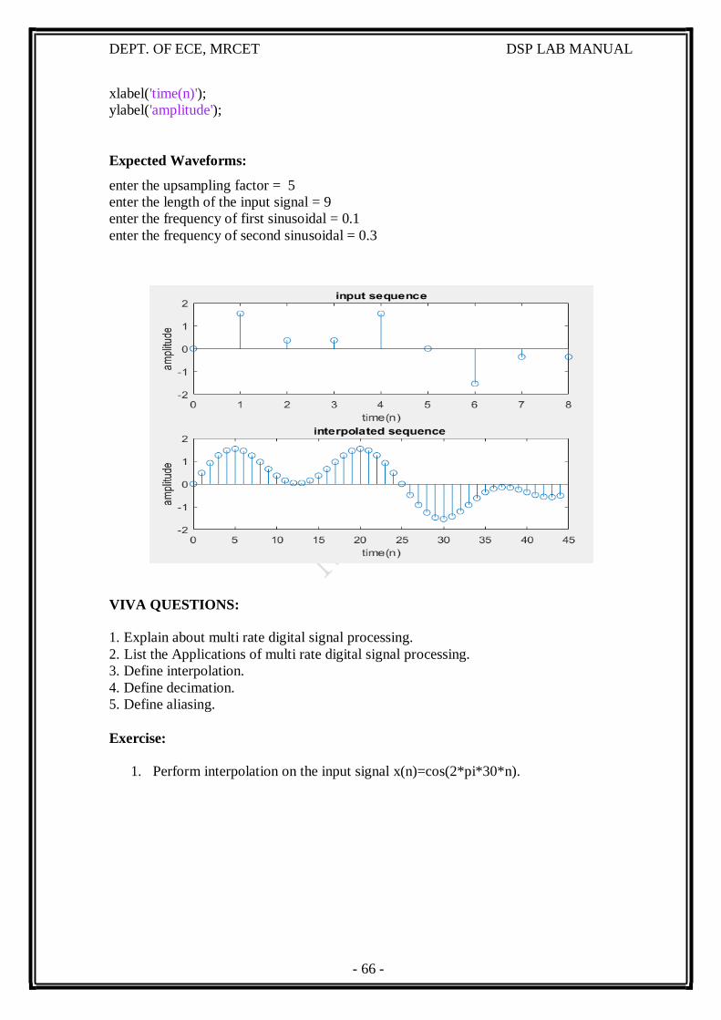
Expected Waveforms:
enter the upsampling factor = 5
enter the length of the input signal = 9
enter the frequency of first sinusoidal = 0.1
enter the frequency of second sinusoidal = 0.3
VIVA QUESTIONS:
1. Explain about multi rate digital signal processing.
2. List the Applications of multi rate digital signal processing.
3. Define interpolation.
4. Define decimation.
5. Define aliasing.
Exercise:
1. Perform interpolation on the input signal x(n)=cos(2*pi*30*n).

- 67 -
DEPT. OF ECE, MRCET DSP LAB MANUAL
OBSEVATIONS
Output Waveforms:
- 68 -
DEPT. OF ECE, MRCET DSP LAB MANUAL
EXP. NO: 15
IMPLEMENTATION OF I/D SAMPLING RATE CONVERTERS
AIM: program to implement sampling rate conversion.
SOFTWARE: MATLAB
THEORY:
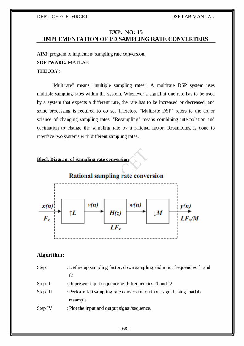
"Multirate" means "multiple sampling rates". A multirate DSP system uses
multiple sampling rates within the system. Whenever a signal at one rate has to be used
by a system that expects a different rate, the rate has to be increased or decreased, and
some processing is required to do so. Therefore "Multirate DSP" refers to the art or
science of changing sampling rates. "Resampling" means combining interpolation and
decimation to change the sampling rate by a rational factor. Resampling is done to
interface two systems with different sampling rates.
Algorithm:
Step I : Define up sampling factor, down sampling and input frequencies f1 and
f2
Step II : Represent input sequence with frequencies f1 and f2
Step III : Perform I/D sampling rate conversion on input signal using matlab
resample
Step IV : Plot the input and output signal/sequence.
Block Diagram of Sampling rate conversion
- 69 -
DEPT. OF ECE, MRCET DSP LAB MANUAL
Flow Chart:
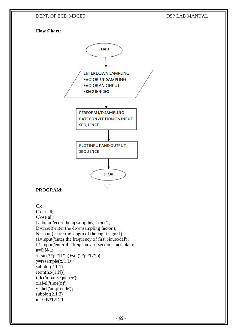
PROGRAM:
Clc;
Clear all;
Close all;
L=input('enter the upsampling factor');
D=input('enter the downsampling factor');
N=input('enter the length of the input signal');
f1=input('enter the frequency of first sinusodal');
f2=input('enter the frequency of second sinusodal');
n=0:N-1;
x=sin(2*pi*f1*n)+sin(2*pi*f2*n);
y=resample(x,L,D);
subplot(2,1,1)
stem(n,x(1:N))
title('input sequence');
xlabel('time(n)');
ylabel('amplitude');
subplot(2,1,2)
m=0:N*L/D-1;
- 70 -
DEPT. OF ECE, MRCET DSP LAB MANUAL
stem(m,y(1:N*L/D));
title('output sequence ');
xlabel('time(n)');
ylabel('amplitude');
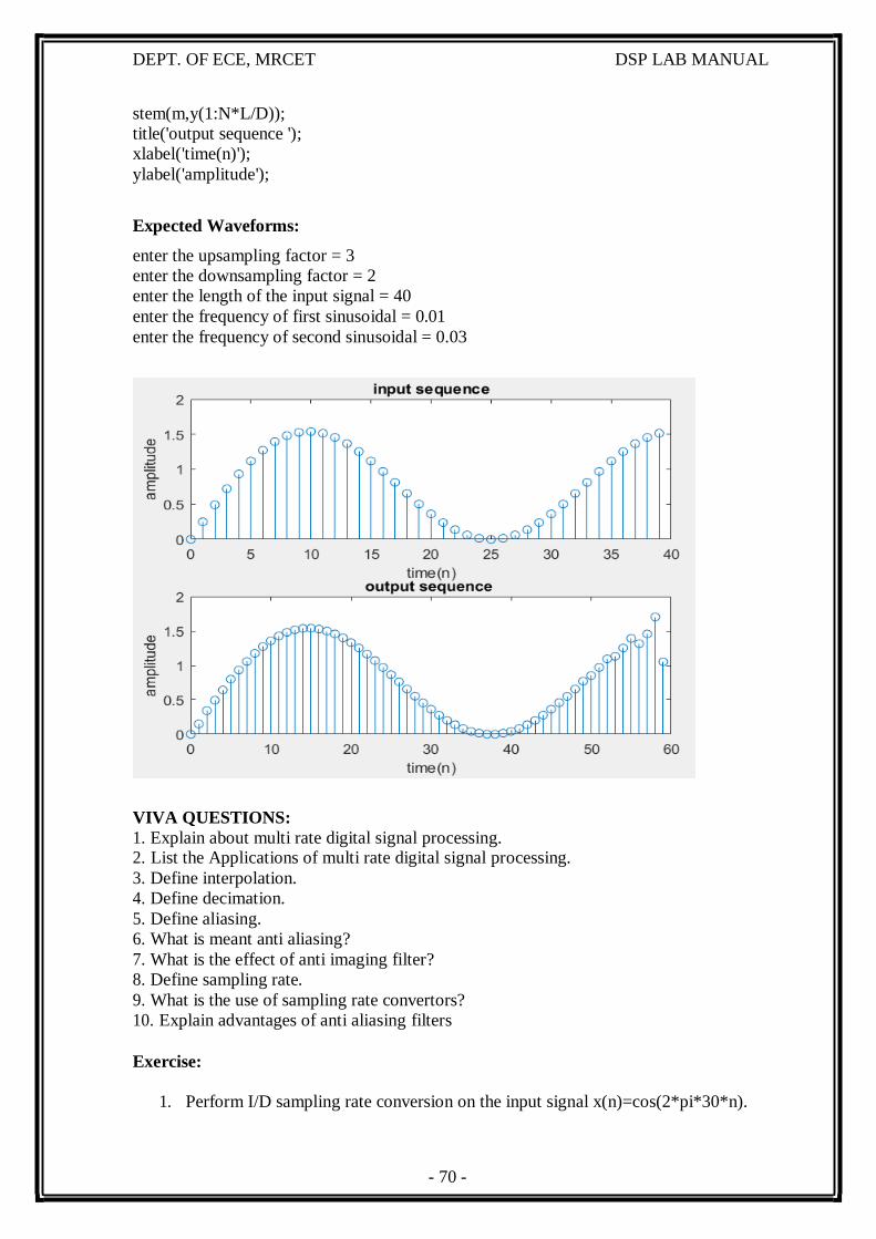
Expected Waveforms:
enter the upsampling factor = 3
enter the downsampling factor = 2
enter the length of the input signal = 40
enter the frequency of first sinusoidal = 0.01
enter the frequency of second sinusoidal = 0.03
VIVA QUESTIONS:
1. Explain about multi rate digital signal processing. 2. List the Applications of multi rate digital signal processing.
3. Define interpolation.
4. Define decimation.
5. Define aliasing.
6. What is meant anti aliasing?
7. What is the effect of anti imaging filter?
8. Define sampling rate.
9. What is the use of sampling rate convertors?
10. Explain advantages of anti aliasing filters
Exercise:
1. Perform I/D sampling rate conversion on the input signal x(n)=cos(2*pi*30*n).
- 71 -
DEPT. OF ECE, MRCET DSP LAB MANUAL
Output Waveforms:
OBSERVATIONS
- 72 -
DEPT. OF ECE, MRCET DSP LAB MANUAL
EXP. NO: 16
IMPULSE RESPONSE OF FIRST ORDER AND SECOND ORDER
SYSTEMS
AIM: program to implement sampling rate conversion.
SOFTWARE: MATLAB
THEORY:
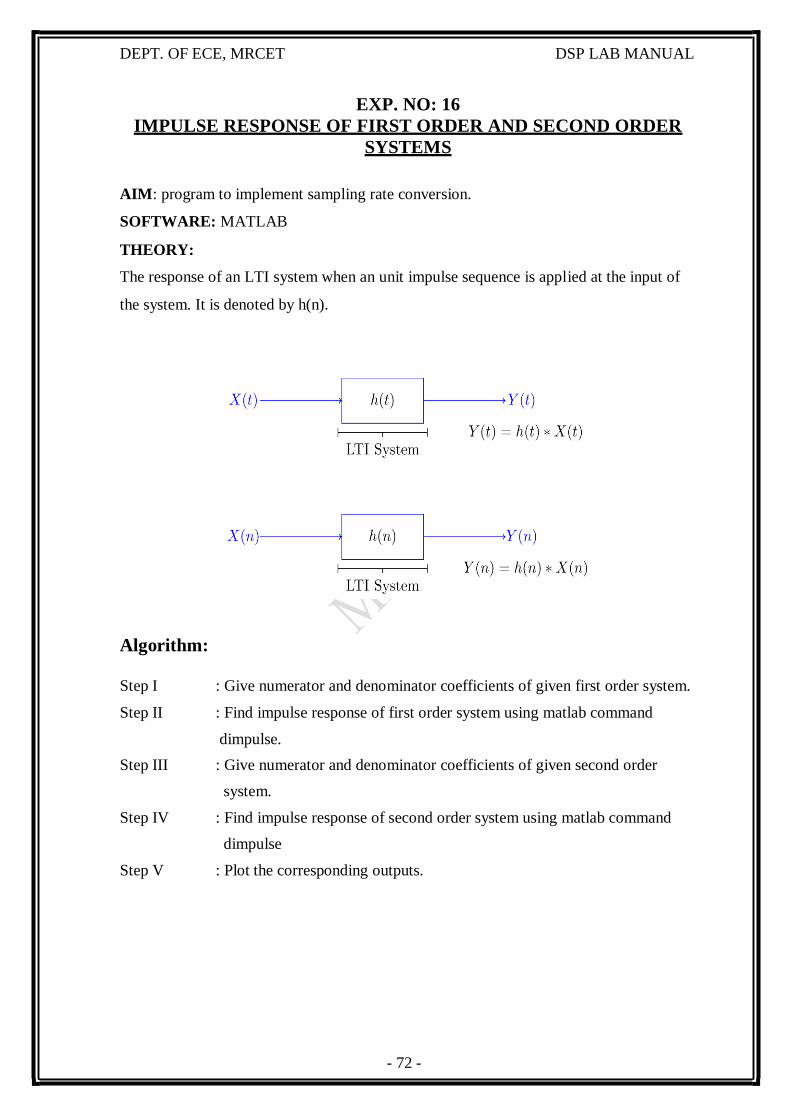
The response of an LTI system when an unit impulse sequence is applied at the input of
the system. It is denoted by h(n).
Algorithm:
Step I : Give numerator and denominator coefficients of given first order system.
Step II : Find impulse response of first order system using matlab command
dimpulse.
Step III : Give numerator and denominator coefficients of given second order
system.
Step IV : Find impulse response of second order system using matlab command
dimpulse
Step V : Plot the corresponding outputs.
- 73 -
DEPT. OF ECE, MRCET DSP LAB MANUAL
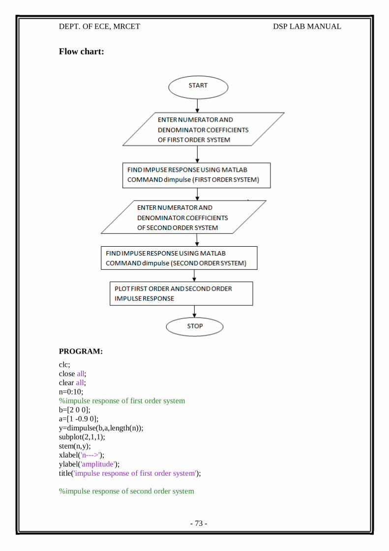
Flow chart:
PROGRAM:
clc;
close all;
clear all;
n=0:10;
%impulse response of first order system
b=[2 0 0];
a=[1 -0.9 0];
y=dimpulse(b,a,length(n));
subplot(2,1,1);
stem(n,y);
xlabel('n--->');
ylabel('amplitude');
title('impulse response of first order system');
%impulse response of second order system
- 74 -
DEPT. OF ECE, MRCET DSP LAB MANUAL
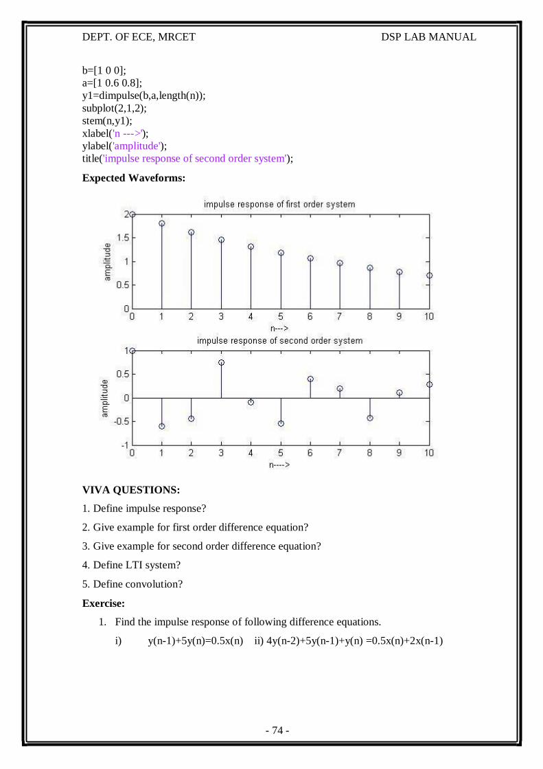
b=[1 0 0];
a=[1 0.6 0.8];
y1=dimpulse(b,a,length(n));
subplot(2,1,2);
stem(n,y1);
xlabel('n --- >');
ylabel('amplitude');
title('impulse response of second order system');
Expected Waveforms:
VIVA QUESTIONS:
1. Define impulse response?
2. Give example for first order difference equation?
3. Give example for second order difference equation?
4. Define LTI system?
5. Define convolution?
Exercise:
1. Find the impulse response of following difference equations.
i) y(n-1)+5y(n)=0.5x(n) ii) 4y(n-2)+5y(n-1)+y(n) =0.5x(n)+2x(n-1)
- 75 -
DEPT. OF ECE, MRCET DSP LAB MANUAL
Output Waveforms:
OBSERVATIONS
- 76 -
DEPT. OF ECE, MRCET DSP LAB MANUAL
PART B - LIST OF EXPERIMENTS USING DSP PROCESSOR
ARCHITECTURE AND INSTRUCTION SET OF
DSPCHIP-TMS320C5515
Introduction to the TMS320C55x:
The TMS320C55x digital signal processor (DSP) represents the latest generation
of ’C5000 DSPs from Texas Instruments. The ’C55x is built on the proven legacy of the
’C54x and is source code compatible with the ’C54x, protecting the customer’s software
investment. Following the trends set by the ’C54x, the ’C55x is optimized for power
efficiency, low system cost, and best-in-class performance for tight power budgets. With
core power dissipation as low as 0.05 mW/MIPS at 0.9V, and performance up to 800
MIPS (400 MHz), the TMS320C55x offers a cost-effective solution to the toughest
challenges in personal and portable processing applications as well as digital
communications infrastructure with restrictive power budgets. Compared to a 120-MHz
’C54x, a 300-MHz ’C55x will deliver approximately 5X higher performance and
dissipate one-sixth the core power dissipation of the ’C54x. The ’C55x core’s ultra-low
power dissipation of 0.05mW/MIPS is achieved through intense attention to low-power
design and advanced power management techniques. The ’C55x designers have
implemented an unparalleled level of power-down configurability and granularity coupled
with unprecedented power management that occurs automatically and is transparent to the
user.
The ’C55x core delivers twice the cycle efficiency of the ’C54x through a dual-
MAC (multiply-accumulate) architecture with parallel instructions, additional
accumulators, ALUs, and data registers. An advanced instruction set, a superset to that of
the ’C54x, combined with expanded busing structure complements the new hardware
execution units. The ’C55x continues the standard set by the ’C54x in code density
leadership for lower system cost. The ’C55x instructions are variable byte lengths ranging
in size from 8 bits to 48 bits. With this scalable instruction word length, the ’C55x can
reduce control code size per function by up to 40% more than ’C54x. Reduced control
code size means reduced memory requirements and lower system cost.
- 77 -
Overview of the C5515 eZdsp USB Stick
DEPT. OF ECE, MRCET DSP LAB MANUAL
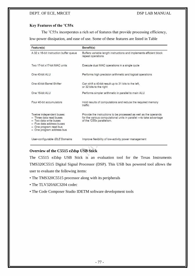
Key Features of the ’C55x
The ’C55x incorporates a rich set of features that provide processing efficiency,
low-power dissipation, and ease of use. Some of these features are listed in Table
The C5515 eZdsp USB Stick is an evaluation tool for the Texas Instruments
TMS320C5515 Digital Signal Processor (DSP). This USB bus powered tool allows the
user to evaluate the following items:
• The TMS320C5515 processor along with its peripherals
• The TLV320AIC3204 codec
• The Code Composer Studio IDETM software development tools
- 78 -
DEPT. OF ECE, MRCET DSP LAB MANUAL
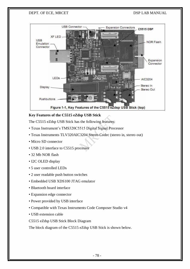
Key Features of the C5515 eZdsp USB Stick
The C5515 eZdsp USB Stick has the following features:
• Texas Instrument’s TMS320C5515 Digital Signal Processor
• Texas Instruments TLV320AIC3204 Stereo Codec (stereo in, stereo out)
• Micro SD connector
• USB 2.0 interface to C5515 processor
• 32 Mb NOR flash
• I2C OLED display
• 5 user controlled LEDs
• 2 user readable push button switches
• Embedded USB XDS100 JTAG emulator
• Bluetooth board interface
• Expansion edge connector
• Power provided by USB interface
• Compatible with Texas Instruments Code Composer Studio v4
• USB extension cable
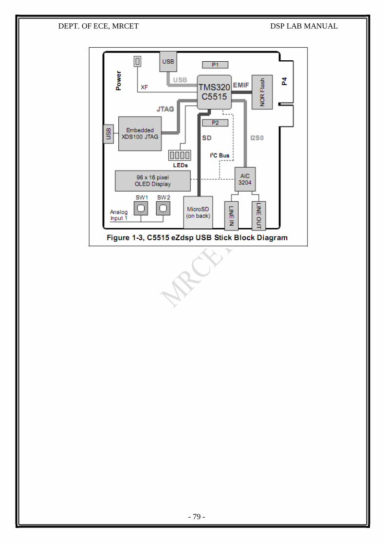
C5515 eZdsp USB Stick Block Diagram
The block diagram of the C5515 eZdsp USB Stick is shown below.
- 79 -
DEPT. OF ECE, MRCET DSP LAB MANUAL
- 80 -
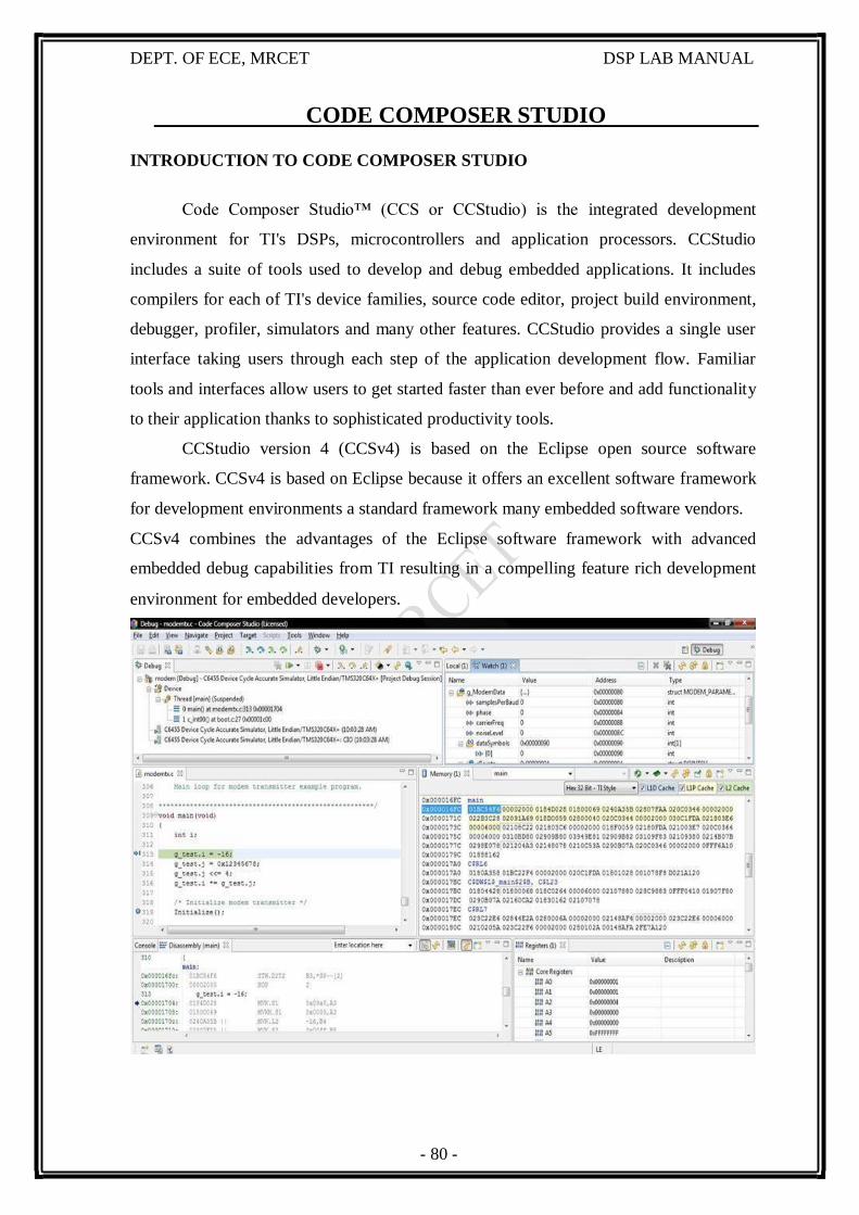
CCSv4 combines the advantages of the Eclipse software framework with advanced
embedded debug capabilities from TI resulting in a compelling feature rich development
environment for embedded developers.
DEPT. OF ECE, MRCET DSP LAB MANUAL
CODE COMPOSER STUDIO
INTRODUCTION TO CODE COMPOSER STUDIO
Code Composer Studio™ (CCS or CCStudio) is the integrated development
environment for TI's DSPs, microcontrollers and application processors. CCStudio
includes a suite of tools used to develop and debug embedded applications. It includes
compilers for each of TI's device families, source code editor, project build environment,
debugger, profiler, simulators and many other features. CCStudio provides a single user
interface taking users through each step of the application development flow. Familiar
tools and interfaces allow users to get started faster than ever before and add functionality
to their application thanks to sophisticated productivity tools.
CCStudio version 4 (CCSv4) is based on the Eclipse open source software
framework. CCSv4 is based on Eclipse because it offers an excellent software framework
for development environments a standard framework many embedded software vendors.
- 81 -
DEPT. OF ECE, MRCET DSP LAB MANUAL
Features
Debugger
CCStudio's integrated debugger has several capabilities and advanced breakpoints
to simplify development. Conditional or hardware breakpoints are based on full C
expressions, local variables or registers. The advanced memory window allows you to
inspect each level of memory so that you can debug complex cache coherency issues.
CCStudio supports the development of complex systems with multiple processors or
cores. Global breakpoints and synchronous operations provide control over multiple
processors and cores.
Profiling
CCStudio's interactive profiler makes it easy to quickly measure code
performance and ensure the efficient use of the target's resources during debug and
development sessions. The profiler allows developers to easily profile all C/C++
functions in their application for instruction cycles or other events such as cache
misses/hits, pipeline stalls and branches.
Profile ranges can be used to concentrate efforts on high-usage areas of code
during optimization, helping developers produce finely-tuned code. Profiling is available
for ranges of assembly, C++ or C code in any combination. To increase productivity, all
profiling facilities are available throughout the development cycle.
Scripting
Some tasks such as testing need to run for hours or days without user interaction.
To accomplish such a task, the IDE should be able to automate common tasks. CCStudio
has a complete scripting environment allowing for the automation of repetitive tasks such
as testing and performance benchmarking. A separate scripting console allows you to type
commands or to execute scripts within the IDE.
Image Analysis and Visualization
CCStudio has many image analysis and graphic visualization. It includes the
ability to graphically view variables and data on displays which can be automatically
refreshed. CCStudio can also look at images and video data in the native format (YUV,
RGB) both in the host PC or loaded in the target board.
- 82 -
DEPT. OF ECE, MRCET DSP LAB MANUAL
Compiler
TI has developed C/C++ compilers specifically tuned to maximize the processor's
usage and performance. TI compilers use a wide range of classical, application-oriented,
and sophisticated device-specific optimizations that are tuned to all the supported
architectures.
Some of these optimizations include:
• Common sub-expression elimination
• Software pipelining
• Strength Reduction
• Auto increment addressing
• Cost-based register allocation
• Instruction predication
• Hardware looping
• Function In-lining
• Vectorization
TI compilers also perform program level optimizations that evaluate code
performance at the application level. With the program level view, the compiler is able to
generate code similar to an assembly program developer who has the full system view.
This application level view is leveraged by the compiler to make trade-offs that
significantly increase the processor performance.
The TI ARM and Microcontroller C/C++ compilers are specifically tuned for code
size and control code efficiency. They offer industry leading performance and
compatibility.
Simulation
Simulators provide a way for users to begin development prior to having access to
a development board. Simulators also have the benefit of providing enhanced visibility
into application performance and behavior. Several simulator variants are available
allowing users to trade off cycle accuracy, speed and peripheral simulation, with some
simulators being ideally suited to algorithm benchmarking and others for more detailed
system simulation. Hardware Debugging (Emulation)
TI devices include advanced hardware debugging capabilities. These capabilities include:
• IEEE 1149.1 (JTAG) and Boundary Scan
• Non-intrusive access to registers and memory
- 83 -
DEPT. OF ECE, MRCET DSP LAB MANUAL
• Real-time mode which provides for the debugging of code that interacts with interrupts
that must not be disabled. Real-time mode allows you to suspend background code at
break events while continuing to execute time-critical interrupt service routines.
• Multi-core operations such as synchronous run, step, and halt. This includes crosscore
triggering, which provides the ability to have one core trigger other cores to halt.
Advanced Event Triggering (AET) which is available on selected devices, allows a user
to halt the CPU or trigger other events based on complex events or sequences such as
invalid data or program memory accesses. It can non-intrusively measure performance
and count system events (for example, cache events).
CCStudio provides Processor Trace on selected devices to help customers find
previously “invisible” complex real-time bugs. Trace can detect the really hard to find
bugs – race conditions between events, intermittent real-time glitches, crashes from stack
overflows, runaway code and false interrupts without stopping the processor. Trace is a
completely nonintrusive debug method that relies on a debug unit inside the processor so
it does not interfere or change the application’s real-time behavior. Trace can fine tune
code performance and cache optimization of complex switch intensive multi-channel
applications. Processor Trace supports the export of program, data, timing and selected
processor and system events/interrupts. Processor Trace can be exported either to an
XDS560 Trace external JTAG emulator, or on selected devices, to an on chip buffer
Embedded Trace Buffer (ETB).
Real time operating system support
CCSv4 comes with two versions of TI's real time operating system:
• DSP/BIOS 5.4x is a real-time operating system that provides pre-emptive multitasking
services for DSP devices. Its services include ISR dispatching, software interrupts,
semaphores, messages, device I/O, memory management, and power management. In
addition, DSP/BIOS 5.x also includes debug instrumentation and tooling, including low-
overhead print and statistics gathering.
• BIOS 6.x is an advanced, extensible real-time operating system that supports ARM926,
ARM Cortex M3, C674x, C64x+, C672x, and 28x-based devices. It offers numerous
kernel and debugging enhancements not available in DSP/BIOS 5.x, including faster,
more flexible memory management, events, and priority-inheritance mutexes.
Note: BIOS 6.x includes a DSP/BIOS 5.x compatibility layer to support easy migration of
application source code.
- 84 -
DEPT. OF ECE, MRCET DSP LAB MANUAL
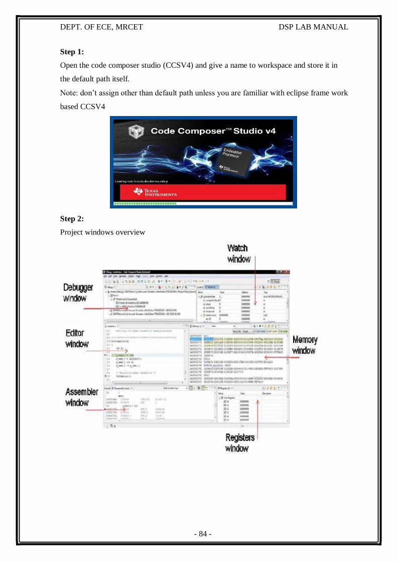
Step 1:
Open the code composer studio (CCSV4) and give a name to workspace and store it in
the default path itself.
Note: don’t assign other than default path unless you are familiar with eclipse frame work
based CCSV4
Step 2:
Project windows overview
- 85 -
read from lookup table
DEPT. OF ECE, MRCET DSP LAB MANUAL
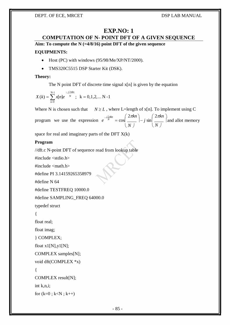
EXP.NO: 1 COMPUTATION OF N- POINT DFT OF A GIVEN SEQUENCE
Aim: To compute the N (=4/8/16) point DFT of the given sequence
EQUIPMENTS:
Host (PC) with windows (95/98/Me/XP/NT/2000).
TMS320C5515 DSP Starter Kit (DSK).
Theory:
The N point DFT of discrete time signal x[n] is given by the equation
N-1
X (k) x[n]e n0
j 2kn
N ; k 0,1,2, ... N -1
Where N is chosen such that N L , where L=length of x[n]. To implement using C
j 2kn 2kn 2kn program we use the expression e N cos j sin and allot memory
N
space for real and imaginary parts of the DFT X(k)
Program
//dft.c N-point DFT of sequence
#include <stdio.h>
#include <math.h>
#define PI 3.14159265358979
#define N 64
#define TESTFREQ 10000.0
#define SAMPLING_FREQ 64000.0
typedef struct
{
float real;
float imag;
} COMPLEX;
float x1[N],y1[N];
COMPLEX samples[N];
void dft(COMPLEX *x)
{
COMPLEX result[N];
int k,n,i;
for (k=0 ; k<N ; k++)
N
- 86 -
DEPT. OF ECE, MRCET DSP LAB MANUAL
{
result[k].real=0.0;
result[k].imag = 0.0;
for (n=0 ; n<N ; n++)
{
result[k].real += x[n].real*cos(2*PI*k*n/N) + x[n].imag*sin(2*PI*k*n/N);
result[k].imag += x[n].imag*cos(2*PI*k*n/N) - x[n].real*sin(2*PI*k*n/N);
}
}
for (k=0 ; k<N ; k++)
{
x[k] = result[k];
}
printf("output");
for (i = 0 ; i < N ; i++) //compute magnitude
{
x1[i] = (int)sqrt(result[i].real*result[i].real + result[i].imag*result[i].imag);
printf("\n%d = %f",i,x1[i]);
}
}
void main() //main function
{
int n;
for(n=0 ; n<N ; n++)
{
y1[n] = samples[n].real = cos(2*PI*TESTFREQ*n/SAMPLING_FREQ);
samples[n].imag = 0.0;
printf("\n%d = %f",n,samples[n].real);
}
printf("real input data stored in array samples[]\n");
printf("\n"); // place breakpoint here
dft(samples); //call DFT function
printf("done!\n");
}
- 87 -
Give Right Click on Your Dft.out file under Binaries and select Load program
Option.
Now Go to Target select Run.
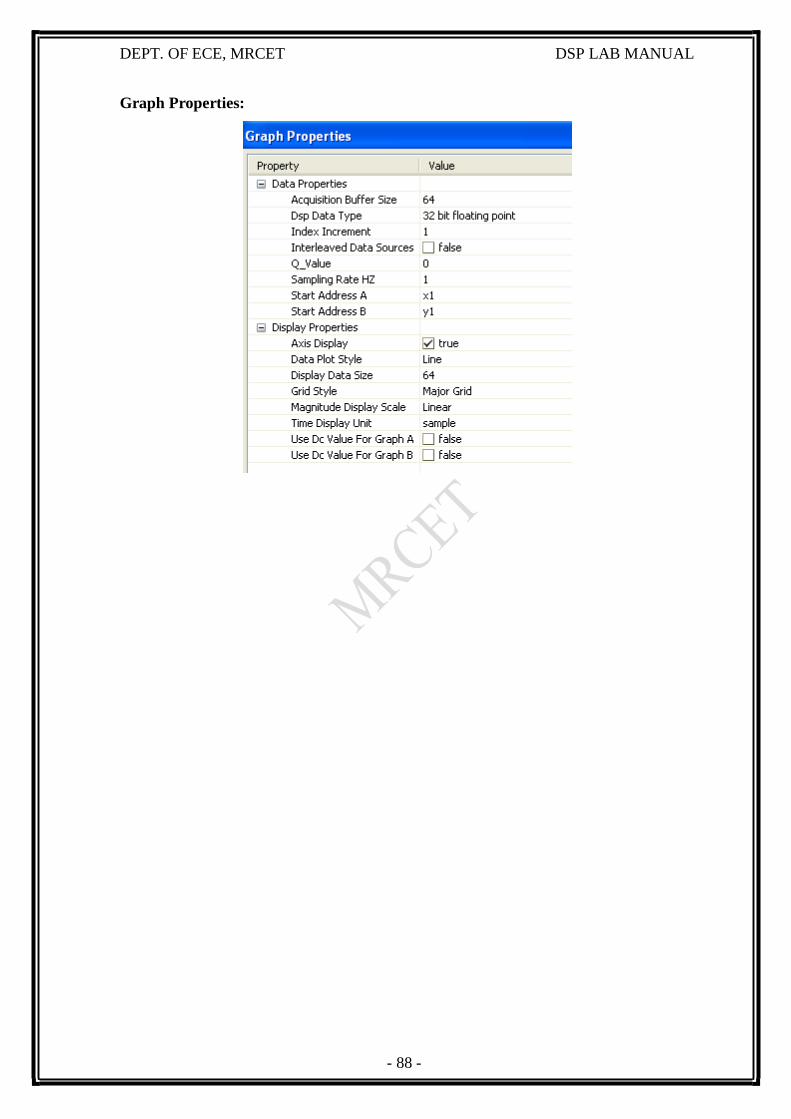
From Tools select Graph(Dual Time) , give properties and select OK.
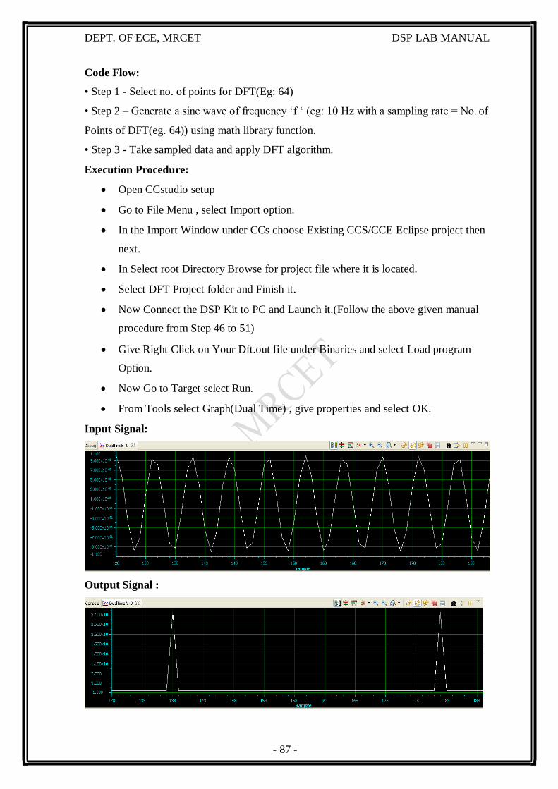
Input Signal:
DEPT. OF ECE, MRCET DSP LAB MANUAL
Code Flow:
• Step 1 - Select no. of points for DFT(Eg: 64)
• Step 2 – Generate a sine wave of frequency ‘f ‘ (eg: 10 Hz with a sampling rate = No. of
Points of DFT(eg. 64)) using math library function.
• Step 3 - Take sampled data and apply DFT algorithm.
Execution Procedure:
Open CCstudio setup
Go to File Menu , select Import option.
In the Import Window under CCs choose Existing CCS/CCE Eclipse project then
next.
In Select root Directory Browse for project file where it is located.
Select DFT Project folder and Finish it.
Now Connect the DSP Kit to PC and Launch it.(Follow the above given manual
procedure from Step 46 to 51)
Output Signal :
- 88 -
DEPT. OF ECE, MRCET DSP LAB MANUAL
Graph Properties:

- 89 -
DEPT. OF ECE, MRCET DSP LAB MANUAL
OBSERVATIONS
Output Waveforms:
- 90 -
DEPT. OF ECE, MRCET DSP LAB MANUAL
EXP.NO: 2 IMPLEMENTATION OF FFT OF GIVEN SEQUENCE
AIM: To compute the FFT of the given sequence
EQUIPMENTS:
1. Host (PC) with windows (95/98/Me/XP/NT/2000).
2. TMS320C5515 DSP Starter Kit (DSK).
FFT Algorithm
The FFT has a fairly easy algorithm to implement, and it is shown step by step in the list
below. This version of the FFT is the Decimation in Time Method
1. Pad input sequence, of N samples, with Zero’s until the number of samples is the
nearest power of two.
e.g. 500 samples are padded to 512 (2^9)
2. Bit reverse the input sequence.
e.g. 3 = 011 goes to 110 = 6
3. Compute (N / 2) two sample DFT's from the shuffled inputs. See "Shuffled Inputs"
4. Compute (N / 4) four sample DFT's from the two sample DFT's. See "Shuffled Inputs"
5. Compute (N / 2) eight sample DFT's from the four sample DFT's. See "Shuffled
Inputs"
6. Until the all the samples combine into one N-sample DFT
PROGRAM:
Main.c
#include "usbstk5515.h"
#include <math.h>
#include <stdio.h>
#define PTS 64 //no of points for FFT
#define PI 3.14159265358979
typedef struct {float real,imag;} COMPLEX;
void FFT(COMPLEX *Y, int n); //FFT prototype
float iobuffer[PTS]; //as input and output buffer
float x1[PTS]; //intermediate buffer
short i; //general purpose index variable
short buffercount = 0; //number of new samples in iobuffer
short flag = 0; //set to 1 by ISR when iobuffer full
COMPLEX w[PTS]; //twiddle constants stored in w
- 91 -
DEPT. OF ECE, MRCET DSP LAB MANUAL
COMPLEX samples[PTS]; //primary working buffer
void main(void)
{
for(i=0;i<PTS;i++)
{
iobuffer[i]=0;
x1[i]=0;
}
printf("\n input");
for (i = 0 ; i<PTS ; i++) // set up twiddle constants in w
{
w[i].real = cos(2*PI*i/(PTS*2.0)); //Re component of twiddle constants
w[i].imag =-sin(2*PI*i/(PTS*2.0)); //Im component of twiddle constants
}
for (i = 0 ; i < PTS ; i++) //swap buffers
{
iobuffer[i] = sin(2*PI*10*i/64.0);/*10- > freq, 64 -> sampling freq*/
printf("\n%d = %f",i,iobuffer[i]);
samples[i].real=0.0;
samples[i].imag=0.0;
}
for (i = 0 ; i < PTS ; i++) //swap buffers
{
samples[i].real=iobuffer[i]; //buffer with new data
}
for (i = 0 ; i < PTS ; i++)
samples[i].imag = 0.0; //imag components = 0
FFT(samples,PTS); //call function FFT.c
printf("\n output");
for (i = 0 ; i < PTS ; i++) //compute magnitude
{
x1[i] = sqrt(samples[i].real*samples[i].real +
samples[i].imag*samples[i].imag);
printf("\n%d = %f",i,x1[i]);
- 92 -
DEPT. OF ECE, MRCET DSP LAB MANUAL
}
} //end of main
fft.c
#define PTS 64 //# of points for FFT
typedef struct {float real,imag;} COMPLEX;
extern COMPLEX w[PTS]; //twiddle constants stored in w
void FFT(COMPLEX *Y, int N) //input sample array, # of points
{
COMPLEX temp1,temp2; //temporary storage variables
int i,j,k; //loop counter variables
int upper_leg, lower_leg; //index of upper/lower butterfly leg
int leg_diff; //difference between upper/lower leg
int num_stages = 0; //number of FFT stages (iterations)
int index, step; //index/step through twiddle constant
i = 1; //log(base2) of N points= # of stages
do
{
num_stages +=1;
i = i*2;
}while (i!=N);
leg_diff = N/2; //difference between upper&lower legs
step = (PTS*2)/N; //step between values in twiddle.h
for (i = 0;i < num_stages; i++) //for N-point FFT
{
index = 0;
for (j = 0; j < leg_diff; j++)
{
for (upper_leg = j; upper_leg < N; upper_leg += (2*leg_diff))
{
lower_leg = upper_leg+leg_diff;
temp1.real = (Y[upper_leg]).real + (Y[lower_leg]).real;
temp1.imag = (Y[upper_leg]).imag + (Y[lower_leg]).imag;
temp2.real = (Y[upper_leg]).real - (Y[lower_leg]).real;
temp2.imag = (Y[upper_leg]).imag - (Y[lower_leg]).imag;
- 93 -
DEPT. OF ECE, MRCET DSP LAB MANUAL
(Y[lower_leg]).real = temp2.real*(w[index]).real
-temp2.imag*(w[index]).imag;
(Y[lower_leg]).imag = temp2.real*(w[index]).imag
+temp2.imag*(w[index]).real;
(Y[upper_leg]).real = temp1.real;
(Y[upper_leg]).imag = temp1.imag;
}
index += step;
}
leg_diff = leg_diff/2;
step *= 2;
}
j = 0;
for (i = 1; i < (N-1); i++) //bit reversal for resequencing data
{
k = N/2;
while (k <= j)
{
j = j - k;
k = k/2;
}
j = j + k;
if (i<j)
{
temp1.real = (Y[j]).real;
temp1.imag = (Y[j]).imag;
(Y[j]).real = (Y[i]).real;
(Y[j]).imag = (Y[i]).imag;
(Y[i]).real = temp1.real;
(Y[i]).imag = temp1.imag;
}
}
return;
}
- 94 -
DEPT. OF ECE, MRCET DSP LAB MANUAL
Code Flow:
• Step 1 - Select no. of points for FFT(Eg: 64)
• Step 2 – Generate a sine wave of frequency ‘f ‘ (eg: 10 Hz with a sampling rate = No. of
Points of FFT(eg. 64)) using math library function.
• Step 3 - Take sampled data and apply FFT algorithm.
Execution Procedure:
Open CCstudio setup
Go to File Menu , select Import option.
In the Import Window under CCs choose Existing CCS/CCE Eclipse project then
next.
In Select root Directory Browse for project file where it is located.
Select FFT Project folder and Finish it.
Now Connect the DSP Kit to PC and Launch it.(Follow the above given manual
procedure from Step 46 to 51)
Give Right Click on Your fft.out file under Binaries and select Load program
Option.
Now Go to Target select Run.
From Tools select Graph(Dual Time) , give properties and select OK.
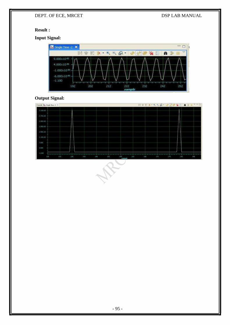
- 95 -
DEPT. OF ECE, MRCET DSP LAB MANUAL
Result :
Input Signal:
Output Signal:

- 96 -
DEPT. OF ECE, MRCET DSP LAB MANUAL
OBSEVATIONS
Output Waveforms:
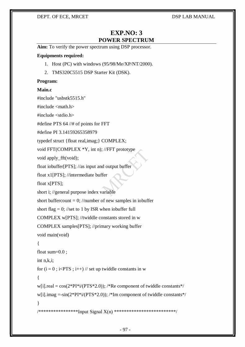
- 97 -
DEPT. OF ECE, MRCET DSP LAB MANUAL
EXP.NO: 3 POWER SPECTRUM
Aim: To verify the power spectrum using DSP processor.
Equipments required:
1. Host (PC) with windows (95/98/Me/XP/NT/2000).
2. TMS320C5515 DSP Starter Kit (DSK).
Program:
Main.c
#include "usbstk5515.h"
#include <math.h>
#include <stdio.h>
#define PTS 64 //# of points for FFT
#define PI 3.14159265358979
typedef struct {float real,imag;} COMPLEX;
void FFT(COMPLEX *Y, int n); //FFT prototype
void apply_fft(void);
float iobuffer[PTS]; //as input and output buffer
float x1[PTS]; //intermediate buffer
float x[PTS];
short i; //general purpose index variable
short buffercount = 0; //number of new samples in iobuffer
short flag = 0; //set to 1 by ISR when iobuffer full
COMPLEX w[PTS]; //twiddle constants stored in w
COMPLEX samples[PTS]; //primary working buffer
void main(void)
{
float sum=0.0 ;
int n,k,i;
for (i = 0 ; i<PTS ; i++) // set up twiddle constants in w
{
w[i].real = cos(2*PI*i/(PTS*2.0)); /*Re component of twiddle constants*/
w[i].imag =-sin(2*PI*i/(PTS*2.0)); /*Im component of twiddle constants*/
}
/****************Input Signal X(n) *************************/
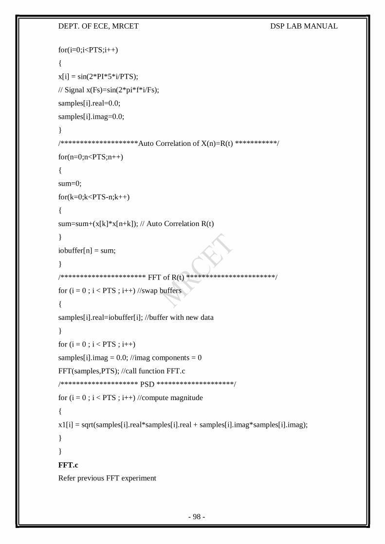
- 98 -
DEPT. OF ECE, MRCET DSP LAB MANUAL
for(i=0;i<PTS;i++)
{
x[i] = sin(2*PI*5*i/PTS);
// Signal x(Fs)=sin(2*pi*f*i/Fs);
samples[i].real=0.0;
samples[i].imag=0.0;
}
/********************Auto Correlation of X(n)=R(t) ***********/
for(n=0;n<PTS;n++)
{
sum=0;
for(k=0;k<PTS-n;k++)
{
sum=sum+(x[k]*x[n+k]); // Auto Correlation R(t)
}
iobuffer[n] = sum;
}
/********************** FFT of R(t) ***********************/
for (i = 0 ; i < PTS ; i++) //swap buffers
{
samples[i].real=iobuffer[i]; //buffer with new data
}
for (i = 0 ; i < PTS ; i++)
samples[i].imag = 0.0; //imag components = 0
FFT(samples,PTS); //call function FFT.c
/******************** PSD ********************/
for (i = 0 ; i < PTS ; i++) //compute magnitude
{
x1[i] = sqrt(samples[i].real*samples[i].real + samples[i].imag*samples[i].imag);
}
}
FFT.c
Refer previous FFT experiment
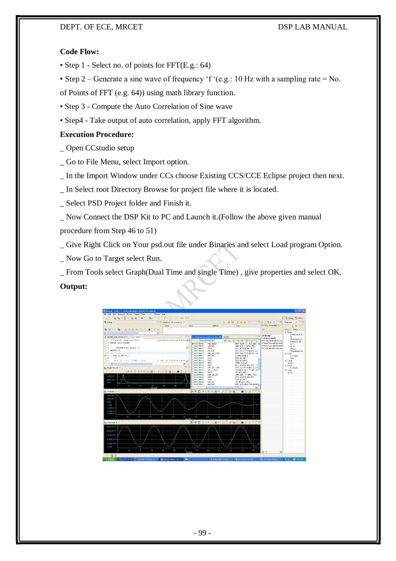
- 99 -
DEPT. OF ECE, MRCET DSP LAB MANUAL
Code Flow:
• Step 1 - Select no. of points for FFT(E.g.: 64)
• Step 2 – Generate a sine wave of frequency ‘f ‘(e.g.: 10 Hz with a sampling rate = No.
of Points of FFT (e.g. 64)) using math library function.
• Step 3 - Compute the Auto Correlation of Sine wave
• Step4 - Take output of auto correlation, apply FFT algorithm.
Execution Procedure:
_ Open CCstudio setup
_ Go to File Menu, select Import option.
_ In the Import Window under CCs choose Existing CCS/CCE Eclipse project then next.
_ In Select root Directory Browse for project file where it is located.
_ Select PSD Project folder and Finish it.
_ Now Connect the DSP Kit to PC and Launch it.(Follow the above given manual
procedure from Step 46 to 51)
_ Give Right Click on Your psd.out file under Binaries and select Load program Option.
_ Now Go to Target select Run.
_ From Tools select Graph(Dual Time and single Time) , give properties and select OK.
Output:

- 100 -
DEPT. OF ECE, MRCET DSP LAB MANUAL
OBSEVATIONS
Output Waveforms:
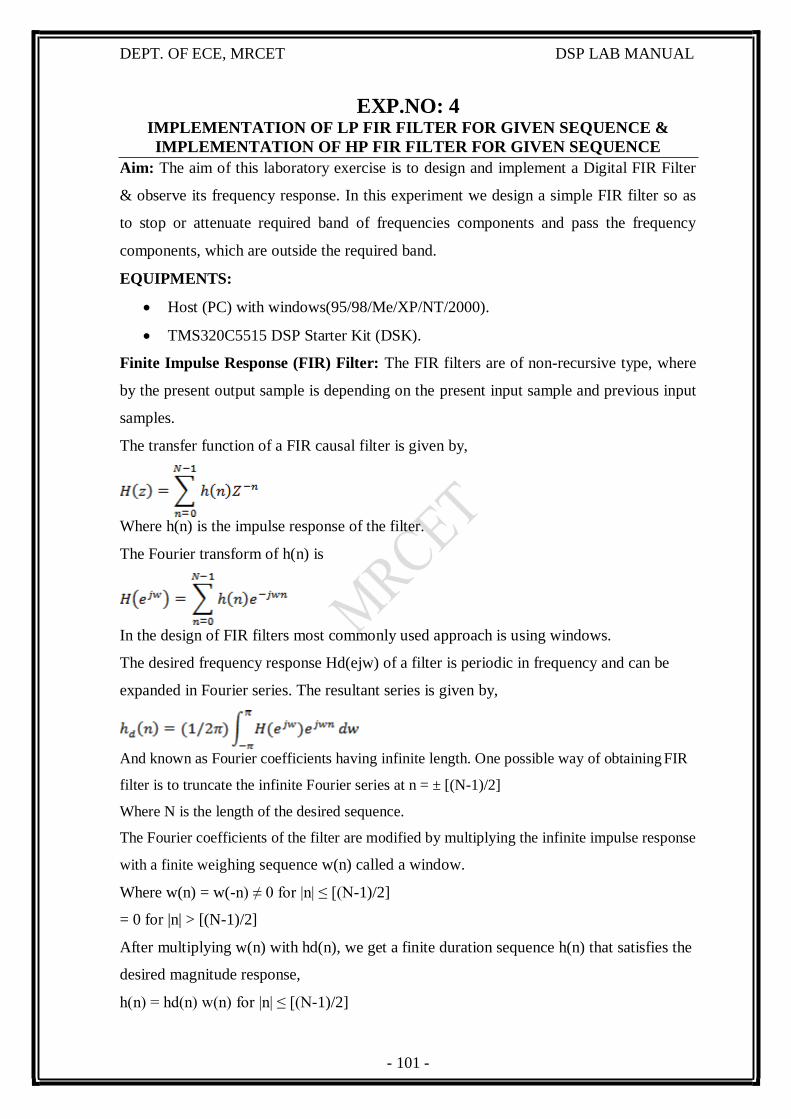
- 101 -
DEPT. OF ECE, MRCET DSP LAB MANUAL
EXP.NO: 4 IMPLEMENTATION OF LP FIR FILTER FOR GIVEN SEQUENCE &
IMPLEMENTATION OF HP FIR FILTER FOR GIVEN SEQUENCE
Aim: The aim of this laboratory exercise is to design and implement a Digital FIR Filter
& observe its frequency response. In this experiment we design a simple FIR filter so as
to stop or attenuate required band of frequencies components and pass the frequency
components, which are outside the required band.
EQUIPMENTS:
Host (PC) with windows(95/98/Me/XP/NT/2000).
TMS320C5515 DSP Starter Kit (DSK).
Finite Impulse Response (FIR) Filter: The FIR filters are of non-recursive type, where
by the present output sample is depending on the present input sample and previous input
samples.
The transfer function of a FIR causal filter is given by,
Where h(n) is the impulse response of the filter.
The Fourier transform of h(n) is
In the design of FIR filters most commonly used approach is using windows.
The desired frequency response Hd(ejw) of a filter is periodic in frequency and can be
expanded in Fourier series. The resultant series is given by,
And known as Fourier coefficients having infinite length. One possible way of obtaining FIR
filter is to truncate the infinite Fourier series at n = ± [(N-1)/2]
Where N is the length of the desired sequence.
The Fourier coefficients of the filter are modified by multiplying the infinite impulse response
with a finite weighing sequence w(n) called a window.
Where w(n) = w(-n) ≠ 0 for |n| ≤ [(N-1)/2]
= 0 for |n| > [(N-1)/2]
After multiplying w(n) with hd(n), we get a finite duration sequence h(n) that satisfies the
desired magnitude response,
h(n) = hd(n) w(n) for |n| ≤ [(N-1)/2]
- 102 -
DEPT. OF ECE, MRCET DSP LAB MANUAL
= 0 for |n| > [(N-1)/2]
The frequency response H(ejw) of the filter can be obtained by convolution of Hd(ejw)
and
W(ejw) is given by,
H(ejw) = Hd(ejw) * W(ejw).
DESIGNING AN FIR FILTER :
Following are the steps to design linear phase FIR filters Using Windowing Method.
I. Clearly specify the filter specifications.
Eg: Order= 30; Sampling Rate= 8000 samples/sec; Cut off Freq. = 400 Hz.
II. Compute the cut-off frequency Wc
Eg: Wc = 2*pie* fc / Fs= 2*pie* 400/8000= 0.1*pie
III. Compute the desired Impulse Response h d (n) using particular Window.
Eg: b_rect1=fir1(order, Wc , 'high',boxcar(31));
IV. Convolve input sequence with truncated Impulse Response x (n)*h (n).
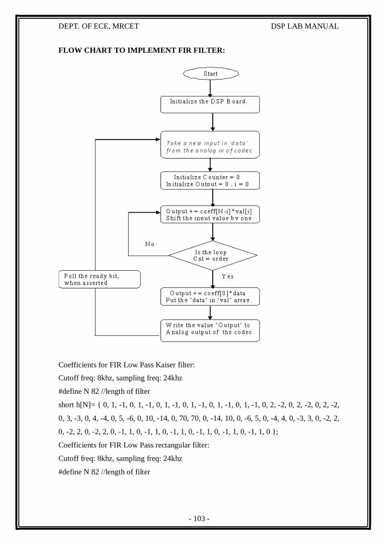
- 103 -
DEPT. OF ECE, MRCET DSP LAB MANUAL
FLOW CHART TO IMPLEMENT FIR FILTER:
Coefficients for FIR Low Pass Kaiser filter:
Cutoff freq: 8khz, sampling freq: 24khz
#define N 82 //length of filter
short h[N]= { 0, 1, -1, 0, 1, -1, 0, 1, -1, 0, 1, -1, 0, 1, -1, 0, 1, -1, 0, 2, -2, 0, 2, -2, 0, 2, -2,
0, 3, -3, 0, 4, -4, 0, 5, -6, 0, 10, -14, 0, 70, 70, 0, -14, 10, 0, -6, 5, 0, -4, 4, 0, -3, 3, 0, -2, 2,
0, -2, 2, 0, -2, 2, 0, -1, 1, 0, -1, 1, 0, -1, 1, 0, -1, 1, 0, -1, 1, 0, -1, 1, 0 };
Coefficients for FIR Low Pass rectangular filter:
Cutoff freq: 8khz, sampling freq: 24khz
#define N 82 //length of filter

- 104 -
DEPT. OF ECE, MRCET DSP LAB MANUAL
short h[N]= { 0, 1, -1, 0, 1, -1, 0, 1, -1, 0, 1, -1, 0, 1, -1, 0, 1, -1, 0, 2, -2, 0, 2, -2, 0, 2, -2,
0, 3, -3, 0, 4, -4, 0, 5, -6, 0, 10, -14, 0, 70, 70, 0, -14, 10, 0, -6, 5, 0, -4, 4, 0, -3, 3, 0, -2, 2,
0, -2, 2, 0, -2, 2, 0, -1, 1, 0, -1, 1, 0, -1, 1, 0, -1, 1, 0, -1, 1, 0, -1, 1, 0 };
Coefficients for FIR Low Pass triangular filter:
Cutoff freq: 8khz, sampling freq: 24khz
#define N 82 //length of filter
short h[N]= { 0, 0, 0, 0, 0, 0, 0, 0, 0, 0, 0, 0, 0, 0, 0, 0, 1, -1, 0, 1, -1, 0, 1, -1, 0, 1, -2, 0, 2,
-2, 0, 3, -3, 0, 5, -6, 0, 9, -13, 0, 70, 70, 0, -13, 9, 0, -6, 5, 0, -3, 3, 0, -2, 2, 0, -2, 1, 0, -1, 1,
0, -1, 1, 0, -1, 1, 0, 0, 0, 0, 0, 0, 0, 0, 0, 0, 0, 0, 0, 0, 0, 0 };
Coefficients for FIR high Pass Kaiser filter:
Cutoff freq: 4khz, sampling freq: 12khz
#define N 82 //length of filter
short h[N]= { 1, 0, -1, 1, -1, -1, 1, -1, -1, 1, -1, -1, 1, -1, -1, 2, -1, -1, 2, -1, -1, 2, -1, -1, 2, -
1, -1, 3, -2, -2, 4, -2, -2, 5, -3, -4, 9, -6, -8, 27, -41, 41, -27, 8, 6, -9, 4, 3, -5, 2, 2, -4, 2, 2, -
3, 1, 1, -2, 1, 1, -2, 1, 1, -2, 1, 1, -2, 1, 1, -1, 1, 1, -1, 1, 1, -1, 1, 1, -1, 1, 0, -1 };
Coefficients for FIR high Pass rectangular filter:
Cutoff freq: 4khz, sampling freq: 12khz
#define N 82 //length of filter
short h[N]= { 1, -1, -1, 1, -1, -1, 1, -1, -1, 1, -1, -1, 1, -1, -1, 2, -1, -1, 2, -1, -1, 2, -1, -1, 2,
-1, -1, 3, -2, -2, 4, -2, -2, 5, -3, -4, 9, -6, -8, 27, -41, 41, -27, 8, 6, -9, 4, 3, -5, 2, 2, -4, 2, 2,
-3, 1, 1, -2, 1, 1, -2, 1, 1, -2, 1, 1, -2, 1, 1, -1, 1, 1, -1, 1, 1, -1, 1, 1, -1, 1, 1, -1 };
Coefficients for FIR high Pass triangular filter:
Cutoff freq: 4khz, sampling freq: 12khz
#define N 82 //length of filter
short h[N]= { 0, 0, 0, 0, 0, 0, 0, 0, 0, 0, 0, 0, 0, 0, 0, 1, 0, 0, 1, 0, -1, 1, -1, -1, 1, -1, -1, 2, -
1, -1, 3, -2, -2, 5, -3, -3, 8, -5, -8, 27, -41, 41, -27, 8, 5, -8, 3, 3, -5, 2, 2, -3, 1, 1, -2, 1, 1, -
1, 1, 1, -1, 1, 0, -1, 0, 0, -1, 0, 0, 0, 0, 0, 0, 0, 0, 0, 0, 0, 0, 0, 0, 0 };
C-Program:
Main.c
#include "stdio.h"
#include "usbstk5515.h"
void main( void )
{
/* Initialize BSL */
- 105 -
DEPT. OF ECE, MRCET DSP LAB MANUAL
USBSTK5515_init();
printf( "playing audio ::::: \n" );
while(1)
{
aic3204_test( );
}
}
Aic3204_test.c:
#define AIC3204_I2C_ADDR 0x18
#include "usbstk5515.h"
#include "usbstk5515_gpio.h"
#include "usbstk5515_i2c.h"
#include "stdio.h"
extern Int16 aic3204_tone_headphone( );
extern Int16 aic3204_loop_stereo_in1( );
Int16 AIC3204_rget( Uint16 regnum, Uint16* regval )
{
Int16 retcode = 0;
Uint8 cmd[2];
cmd[0] = regnum & 0x007F; // 7-bit Register Address
cmd[1] = 0;
retcode |= USBSTK5515_I2C_write( AIC3204_I2C_ADDR, cmd, 1 );
retcode |= USBSTK5515_I2C_read( AIC3204_I2C_ADDR, cmd, 1 );
*regval = cmd[0];
USBSTK5515_wait( 10 );
return retcode;
}
Int16 AIC3204_rset( Uint16 regnum, Uint16 regval )
{
Uint8 cmd[2];
cmd[0] = regnum & 0x007F; // 7-bit Register Address
cmd[1] = regval; // 8-bit Register Data
return USBSTK5515_I2C_write( AIC3204_I2C_ADDR, cmd, 2 );
}
- 106 -
DEPT. OF ECE, MRCET DSP LAB MANUAL
Int16 aic3204_test( )
{
SYS_EXBUSSEL = 0x6100; // Enable I2C bus
USBSTK5515_I2C_init( ); // Initialize I2C
USBSTK5515_wait( 100 ); // Wait
if ( aic3204_loop_stereo_in1( ) )
return 1;
return 0;
}
aic3204_loop_stereo_in1.c:
#include "stdio.h"
#include "usbstk5515.h"
extern Int16 AIC3204_rset( Uint16 regnum, Uint16 regval);
#define Rcv 0x08
#define Xmit 0x20
#define N 82
Int16 data1, data2, data3, data4;
int sample,n,k,l;
Int16 dly0[N];
Int32 lyn,ryn;
/*//hpkaiser12-4
Int16 h[N]= {1, 0, -1, 1, -1, -1, 1, -1, -1, 1, -1, -1, 1, -1, -1, 2, -1, -1, 2, -1, -1, 2, -1, -1,
2, -1, -1, 3, -2, -2, 4, -2, -2, 5, -3, -4, 9, -6, -8, 27, -41, 41, -27, 8, 6, -9, 4, 3, -5, 2, 2, -4, 2,
2, -3, 1, 1, -2, 1, 1, -2, 1, 1, -2, 1, 1, -2, 1, 1, -1, 1, 1, -1, 1, 1, -1, 1, 1, -1, 1, 0, -1 };*/
/*//hprect12-4
Int16 h[N]= { 1, -1, -1, 1, -1, -1, 1, -1, -1, 1, -1, -1, 1, -1, -1, 2, -1, -1, 2, -1, -1, 2, -1, -1,
2, -1, -1, 3, -2, -2, 4, -2, -2, 5, -3, -4, 9, -6, -8, 27, -41, 41, -27, 8, 6, -9, 4, 3, -5, 2, 2, -4, 2,
2, -3, 1, 1, -2, 1, 1, -2, 1, 1, -2, 1, 1, -2, 1, 1, -1, 1, 1, -1, 1, 1, -1, 1, 1, -1, 1, 1, -1 };*/
/*//hptrig12-4
Int16 h[N]= { 0, 0, 0, 0, 0, 0, 0, 0, 0, 0, 0, 0, 0, 0, 0, 1, 0, 0, 1, 0, -1, 1, -1, -1, 1, -1, -1, 2, -
1, -1, 3, -2, -2, 5, -3, -3, 8, -5, -8, 27, -41, 41, -27, 8, 5, -8, 3, 3, -5, 2, 2, -3, 1, 1, -2, 1, 1, -
1, 1, 1,-1, 1, 0, -1, 0, 0, -1, 0, 0, 0, 0, 0,0, 0, 0, 0, 0, 0, 0, 0, 0, 0};*/
/*//lpkaiser24-8
- 107 -
DEPT. OF ECE, MRCET DSP LAB MANUAL
Int16 h[N]= {0, 1, -1, 0, 1, -1, 0, 1, -1, 0, 1, -1,0, 1, -1, 0, 1, -1, 0, 2, -2, 0, 2, -2,0, 2, -2, 0,
3, -3, 0, 4, -4, 0, 5, -6, 0, 10, -14, 0, 70, 70, 0, -14, 10, 0, -6, 5, 0, -4, 4, 0, -3, 3, 0, -2, 2, 0,
-2, 2,0, -2, 2, 0, -1, 1, 0, -1, 1, 0, -1, 1,0, -1, 1, 0, -1, 1, 0, -1, 1, 0 };*/
/*//lprect24-8
short h[N]= {0, 1, -1, 0, 1, -1, 0, 1, -1, 0, 1, -1,0, 1, -1, 0, 1, -1, 0, 2, -2, 0, 2, -2,0, 2, -2, 0,
3, -3, 0, 4, -4, 0, 5, -6,0, 10, -14, 0, 70, 70, 0, -14, 10, 0, -6, 5, 0, -4, 4, 0, -3, 3, 0, -2, 2, 0, -
2, 2,0, -2, 2, 0, -1, 1, 0, -1, 1, 0, -1, 1,0, -1, 1, 0, -1, 1, 0, -1, 1, 0 };*/
/*//lptrig24-8
Int16 h[N]= { 0, 0, 0, 0, 0, 0, 0, 0, 0, 0, 0, 0, 0, 0, 0, 0, 1, -1, 0, 1, -1, 0, 1, -1, 0, 1, -2, 0, 2,
-2, 0, 3, -3, 0, 5, -6,0, 9, -13, 0, 70, 70, 0, -13, 9, 0, -6, 5,0, -3, 3, 0, -2, 2, 0, -2, 1, 0, -1, 1,
0, -1, 1, 0, -1, 1, 0, 0, 0, 0, 0, 0,0, 0, 0, 0, 0, 0, 0, 0, 0, 0};*/
//lpkaiser48-8
Int16 h[N]= {-1, 0, 1, 1, 1, -1, -1, -1, 1, 1, 1, -1,-1, -1, 1, 2, 1, -1, -2, -1, 1, 2, 1, -1, -2, -1,
1, 3, 2, -2, -4, -2, 2, 5, 3, -4,-9, -6, 8, 27, 41, 41, 27, 8, -6, -9, -4, 3,5, 2, -2, -4, -2, 2, 3, 1, -
1, -2, -1, 1,2, 1, -1, -2, -1, 1, 2, 1, -1, -1, -1, 1,1, 1, -1, -1, -1, 1, 1, 1, 0, -1};
Int16 aic3204_loop_stereo_in1( )
{
Int16 j, i = 0;
/* Configure AIC3204 */
AIC3204_rset( 0, 0 ); // Select page 0
AIC3204_rset( 1, 1 ); // Reset codec
AIC3204_rset( 0, 1 ); // Point to page 1
AIC3204_rset( 1, 8 ); // Disable crude AVDD generation from DVDD
AIC3204_rset( 2, 1 ); // Enable Analog Blocks, use LDO power
AIC3204_rset( 0, 0 ); // Select page 0
/* PLL and Clocks config and Power Up */
AIC3204_rset( 27, 0x0d ); // BCLK and WCLK is set as o/p to AIC3204(Master)
AIC3204_rset( 28, 0x00 ); // Data ofset = 0
AIC3204_rset( 4, 3 ); // PLL setting: PLLCLK <- MCLK, CODEC_CLKIN <-PLL CLK
AIC3204_rset( 6, 8 ); // PLL setting: J=8
AIC3204_rset( 7, 15 ); // PLL setting: HI_BYTE(D)
AIC3204_rset( 8, 0xdc ); // PLL setting: LO_BYTE(D)
AIC3204_rset( 30, 0x88 ); // For 32 bit clocks per frame in Master mode ONLY
// BCLK=DAC_CLK/N =(12288000/8) = 1.536MHz = 32*fs
- 108 -
DEPT. OF ECE, MRCET DSP LAB MANUAL
AIC3204_rset( 5, 0x91 ); // PLL setting: Power up PLL, P=1 and R=1
AIC3204_rset( 13, 0 ); // Hi_Byte(DOSR) for DOSR = 128 decimal or 0x0080 DAC
oversamppling
AIC3204_rset( 14, 0x80 ); // Lo_Byte(DOSR) for DOSR = 128 decimal or 0x0080
AIC3204_rset( 20, 0x80 ); // AOSR for AOSR = 128 decimal or 0x0080 for decimation
filters 1 to 6
AIC3204_rset( 11, 0x88 ); // Power up NDAC and set NDAC value to 8
AIC3204_rset( 12, 0x82 ); // Power up MDAC and set MDAC value to 2
AIC3204_rset( 18, 0x88 ); // Power up NADC and set NADC value to 8
AIC3204_rset( 19, 0x82 ); // Power up MADC and set MADC value to 2
/* DAC ROUTING and Power Up */
AIC3204_rset( 0, 0x01 ); // Select page 1
AIC3204_rset( 12, 0x08 ); // LDAC AFIR routed to HPL
AIC3204_rset( 13, 0x08 ); // RDAC AFIR routed to HPR
AIC3204_rset( 0, 0x00 ); // Select page 0
AIC3204_rset( 64, 0x02 ); // Left vol=right vol
AIC3204_rset( 65, 0x00 ); // Left DAC gain to 0dB VOL; Right tracks Left
AIC3204_rset( 63, 0xd4 ); // Power up left,right data paths and set channel
AIC3204_rset( 0, 0x01 ); // Select page 1
AIC3204_rset( 16, 0x06 ); // Unmute HPL , 6dB gain
AIC3204_rset( 17, 0x06 ); // Unmute HPR , 6dB gain
AIC3204_rset( 9, 0x30 ); // Power up HPL,HPR
AIC3204_rset( 0, 0x00 ); // Select page 0
USBSTK5515_wait( 500 ); // Wait
/* ADC ROUTING and Power Up */
AIC3204_rset( 0, 1 ); // Select page 1
AIC3204_rset( 0x34, 0x30 ); // STEREO 1 Jack
// IN2_L to LADC_P through 40 kohm
AIC3204_rset( 0x37, 0x30 ); // IN2_R to RADC_P through 40 kohmm
AIC3204_rset( 0x36, 3 ); // CM_1 (common mode) to LADC_M through 40 kohm
AIC3204_rset( 0x39, 0xc0 ); // CM_1 (common mode) to RADC_M through 40 kohm
AIC3204_rset( 0x3b, 0 ); // MIC_PGA_L unmute
AIC3204_rset( 0x3c, 0 ); // MIC_PGA_R unmute
AIC3204_rset( 0, 0 ); // Select page 0
- 109 -
DEPT. OF ECE, MRCET DSP LAB MANUAL
AIC3204_rset( 0x51, 0xc0 ); // Powerup Left and Right ADC
AIC3204_rset( 0x52, 0 ); // Unmute Left and Right ADC
AIC3204_rset( 0, 0 );
USBSTK5515_wait( 200 ); // Wait
/* I2S settings */
I2S0_SRGR = 0x0;
I2S0_CR = 0x8010; // 16-bit word, slave, enable I2C
I2S0_ICMR = 0x3f; // Enable interrupts
/* Play Tone */
for(l=0;l<N;l++)
dly0[l]=0;
for ( i = 0 ; i < 5 ; i++ )
{
for ( j = 0 ; j < 1000 ; j++ )
{
for ( sample = 0 ; sample < N ; sample++ )
{
/* Read Digital audio input */
data3 = I2S0_W0_MSW_R; // 16 bit left channel received audio data
data1 = I2S0_W0_LSW_R;
data4 = I2S0_W1_MSW_R; // 16 bit right channel received audio data
data2 = I2S0_W1_LSW_R;
while((Rcv & I2S0_IR) == 0); // Wait for interrupt pending flag
lyn=0;
for(k=0;k<N;k++)
{
dly0[(N-1)-k]=dly0[(N-1)-k-1];
dly0[0]=data3;
}
for(k=0;k<N;k++)
lyn+=((h[k])*dly0[k]); //fir low pass filter
data1=lyn>>1;
data2=data1;
/* Write Digital audio input */
- 110 -
DEPT. OF ECE, MRCET DSP LAB MANUAL
I2S0_W0_MSW_W = data1; // 16 bit left channel transmit audio data
I2S0_W0_LSW_W = 0;
I2S0_W1_MSW_W = data2; // 16 bit right channel transmit audio data
I2S0_W1_LSW_W = 0;
while((Xmit & I2S0_IR) == 0); // Wait for interrupt pending flag
}
}
}
/* Disble I2S */
I2S0_CR = 0x00;
return 0;
}
Execution Procedure:
Open CCstudio setup
Go to File Menu , select Import option.
In the Import Window under CCs choose Existing CCS/CCE Eclipse project then
next.
In Select root Directory Browse for project file where it is located.
Select FIR Project folder and Finish it.
Now Connect the DSP Kit to PC and Launch it.(Follow the above given manual
procedure from Step 46 to 51)
Give Right Click on Your fir.out file under Binaries and select Load program
Option.
Now Go to Target select Run.
Observe the audio (Give Input from Stereo in and listen Filtered Output from
Stereo Out).

- 111 -
DEPT. OF ECE, MRCET DSP LAB MANUAL
OBSEVATIONS
Output Waveforms:
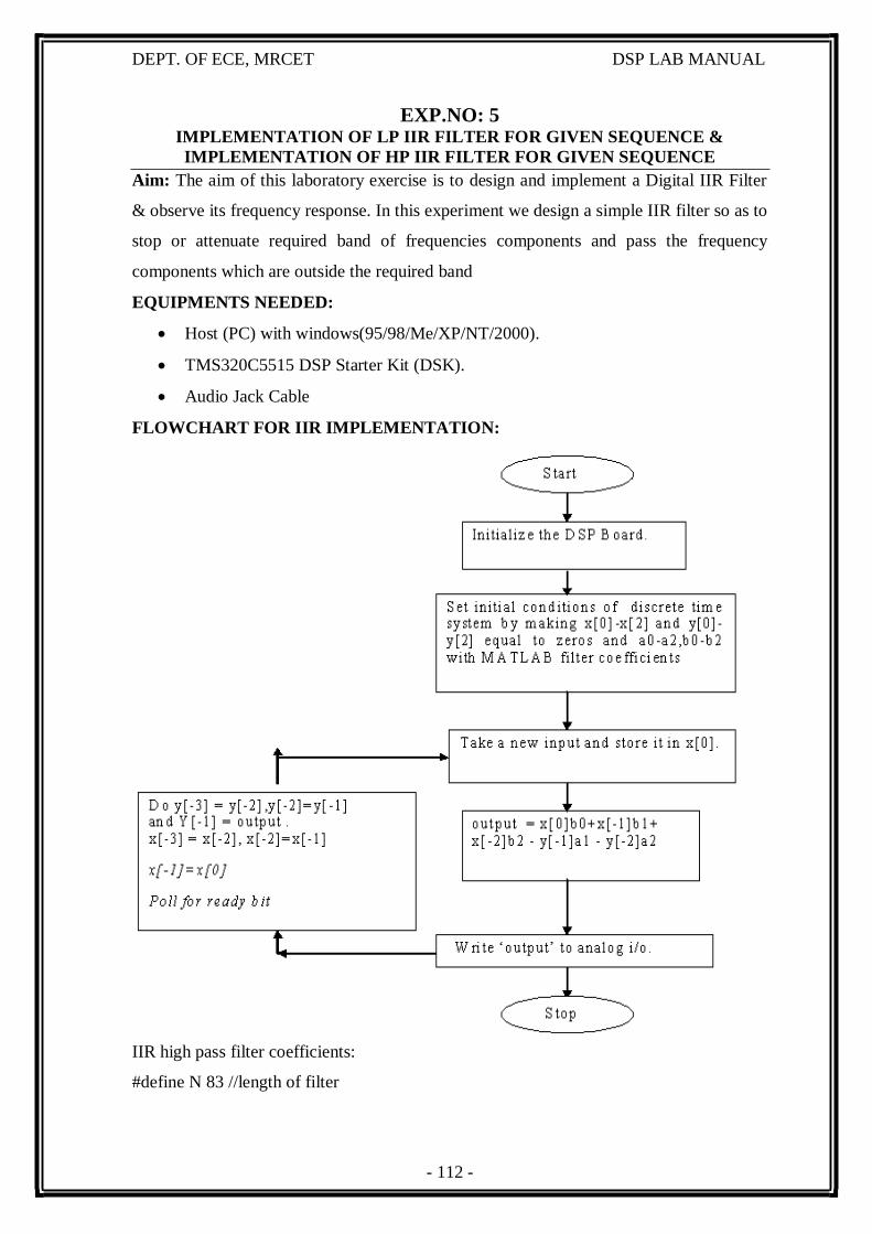
- 112 -
DEPT. OF ECE, MRCET DSP LAB MANUAL
EXP.NO: 5 IMPLEMENTATION OF LP IIR FILTER FOR GIVEN SEQUENCE &
IMPLEMENTATION OF HP IIR FILTER FOR GIVEN SEQUENCE
Aim: The aim of this laboratory exercise is to design and implement a Digital IIR Filter
& observe its frequency response. In this experiment we design a simple IIR filter so as to
stop or attenuate required band of frequencies components and pass the frequency
components which are outside the required band
EQUIPMENTS NEEDED:
Host (PC) with windows(95/98/Me/XP/NT/2000).
TMS320C5515 DSP Starter Kit (DSK).
Audio Jack Cable
FLOWCHART FOR IIR IMPLEMENTATION:
IIR high pass filter coefficients:
#define N 83 //length of filter
- 113 -
DEPT. OF ECE, MRCET DSP LAB MANUAL
Short h[N]={1,3,1,3,1,3,1,3,1,3,1,3,1,3,1,3,1,3,1,3,1,3,1,3,1,3,1,3,1,3,1,3,1,3,1,
3,1,3,1,3,1,3,1,3,1,3,1,3,1,3,1,3,1,3,1,3,1,3,1,3,1,3,1,3,1,3,1,3,1,3,1, 1,3,1,3,1,3,1,3,1,2,1};
IIR low pass filter coefficients:
#define N 83 //length of filter
Shorth[N]={1,3,1,3,1,3,1,3,1,3,1,3,1,3,1,3,1,3,1,3,1,3,1,3,1,3,1,3,1,3,1,3,1,3,1,3,1,3,1,3,1,
3,1,3,1,3,1,3,1,3,1,3,1,3,1,3,1,3,1,3,1,3,1,3,1,3,1,3,1,3,1,3,1,3,1,3,1,3,1,3,1,2,1 };
rogram:
main.c
#include "stdio.h"
#include "usbstk5515.h"
void main( void )
{
/* Initialize BSL */
USBSTK5515_init();
printf( "playing audio ::::: \n" );
while(1)
{
aic3204_test( );
}
}
Aic3204_test.c:
#define AIC3204_I2C_ADDR 0x18
#include "usbstk5515.h"
#include "usbstk5515_gpio.h"
#include "usbstk5515_i2c.h"
#include "stdio.h"
extern Int16 aic3204_tone_headphone( );
extern Int16 aic3204_loop_stereo_in1( );
Int16 AIC3204_rget( Uint16 regnum, Uint16* regval )
{
Int16 retcode = 0;
Uint8 cmd[2];
cmd[0] = regnum & 0x007F; // 7-bit Register Address
cmd[1] = 0;
- 114 -
DEPT. OF ECE, MRCET DSP LAB MANUAL
retcode |= USBSTK5515_I2C_write( AIC3204_I2C_ADDR, cmd, 1 );
retcode |= USBSTK5515_I2C_read( AIC3204_I2C_ADDR, cmd, 1 );
*regval = cmd[0];
USBSTK5515_wait( 10 );
return retcode;
}
Int16 AIC3204_rset( Uint16 regnum, Uint16 regval )
{
Uint8 cmd[2];
cmd[0] = regnum & 0x007F; // 7-bit Register Address
cmd[1] = regval; // 8-bit Register Data
return USBSTK5515_I2C_write( AIC3204_I2C_ADDR, cmd, 2 );
}
Int16 aic3204_test( )
{
SYS_EXBUSSEL = 0x6100; // Enable I2C bus
USBSTK5515_I2C_init( ); // Initialize I2C
USBSTK5515_wait( 100 ); // Wait
if ( aic3204_loop_stereo_in1( ) )
return 1;
return 0;
}
aic3204_loop_stereo_in1.c:
#include "stdio.h"
#include "usbstk5515.h"
extern Int16 AIC3204_rset( Uint16 regnum, Uint16 regval);
#define Rcv 0x08
#define Xmit 0x20
#define N 83
Int16 data1, data2, data3, data4;
int sample, n, k, l;
Int16 dly0[N];
Int16 dly1[N];
Int32 lyn,lyn0,lyn1;
- 115 -
DEPT. OF ECE, MRCET DSP LAB MANUAL
Int16 h[N]={1,3,1,3,1,3,1,3,1,3,1,3,1,3,1,3,1,3,1,3,1,3,1,3,1,3,1,3,1,3,1,3,1,3,1,
3,1,3,1,3,1,3,1,3,1,3,1,3,1,3,1,3,1,3,1,3,1,3,1,3,1,3,1,3,1,3,1,3,1,3,1, 3,1,3,1,3,1,3,1,3,1,2,1
};
Int16 aic3204_loop_stereo_in1 ( )
{
/* Pre-generated sine wave data, 16-bit signed samples */
Int16 j, i = 0;
/* Configure AIC3204 */
AIC3204_rset( 0, 0 ); // Select page 0
AIC3204_rset( 1, 1 ); // Reset codec
AIC3204_rset( 0, 1 ); // Point to page 1
AIC3204_rset( 1, 8 ); // Disable crude AVDD generation from DVDD
AIC3204_rset( 2, 1 ); // Enable Analog Blocks, use LDO power
AIC3204_rset( 0, 0 ); // Select page 0
/* PLL and Clocks config and Power Up */
AIC3204_rset( 27, 0x0d ); // BCLK and WCLK is set as o/p to AIC3204(Master)
AIC3204_rset( 28, 0x00 ); // Data ofset = 0
AIC3204_rset( 4, 3 ); // PLL setting: PLLCLK <- MCLK, CODEC_CLKIN <-PLL
CLK
AIC3204_rset( 6, 8 ); // PLL setting: J=8
AIC3204_rset( 7, 15 ); // PLL setting: HI_BYTE(D)
AIC3204_rset( 8, 0xdc ); // PLL setting: LO_BYTE(D)
AIC3204_rset( 30, 0x88 ); // For 32 bit clocks per frame in Master mode ONLY
// BCLK=DAC_CLK/N =(12288000/8) = 1.536MHz = 32*fs
AIC3204_rset( 5, 0x91 ); // PLL setting: Power up PLL, P=1 and R=1
AIC3204_rset( 13, 0 ); // Hi_Byte(DOSR) for DOSR = 128 decimal or 0x0080 DAC
oversamppling
AIC3204_rset( 14, 0x80 ); // Lo_Byte(DOSR) for DOSR = 128 decimal or 0x0080
AIC3204_rset( 20, 0x80 ); // AOSR for AOSR = 128 decimal or 0x0080 for decimation
filters 1 to 6
AIC3204_rset( 11, 0x88 ); // Power up NDAC and set NDAC value to 8
AIC3204_rset( 12, 0x82 ); // Power up MDAC and set MDAC value to 2
AIC3204_rset( 18, 0x88 ); // Power up NADC and set NADC value to 8
AIC3204_rset( 19, 0x82 ); // Power up MADC and set MADC value to 2
- 116 -
DEPT. OF ECE, MRCET DSP LAB MANUAL
/* DAC ROUTING and Power Up */
AIC3204_rset( 0, 0x01 ); // Select page 1
AIC3204_rset( 12, 0x08 ); // LDAC AFIR routed to HPL
AIC3204_rset( 13, 0x08 ); // RDAC AFIR routed to HPR
AIC3204_rset( 0, 0x00 ); // Select page 0
AIC3204_rset( 64, 0x02 ); // Left vol=right vol
AIC3204_rset( 65, 0x00 ); // Left DAC gain to 0dB VOL; Right tracks Left
AIC3204_rset( 63, 0xd4 ); // Power up left,right data paths and set channel
AIC3204_rset( 0, 0x01 ); // Select page 1
AIC3204_rset( 16, 0x06 ); // Unmute HPL , 6dB gain
AIC3204_rset( 17, 0x06 ); // Unmute HPR , 6dB gain
AIC3204_rset( 9, 0x30 ); // Power up HPL,HPR
AIC3204_rset( 0, 0x00 ); // Select page 0
USBSTK5515_wait( 500 ); // Wait
/* ADC ROUTING and Power Up */
AIC3204_rset( 0, 1 ); // Select page 1
AIC3204_rset( 0x34, 0x30 ); // STEREO 1 Jack
// IN2_L to LADC_P through 40 kohm
AIC3204_rset( 0x37, 0x30 ); // IN2_R to RADC_P through 40 kohmm
AIC3204_rset( 0x36, 3 ); // CM_1 (common mode) to LADC_M through 40 kohm
AIC3204_rset( 0x39, 0xc0 ); // CM_1 (common mode) to RADC_M through 40 kohm
AIC3204_rset( 0x3b, 0 ); // MIC_PGA_L unmute
AIC3204_rset( 0x3c, 0 ); // MIC_PGA_R unmute
AIC3204_rset( 0, 0 ); // Select page 0
AIC3204_rset( 0x51, 0xc0 ); // Powerup Left and Right ADC
AIC3204_rset( 0x52, 0 ); // Unmute Left and Right ADC
AIC3204_rset( 0, 0 );
USBSTK5515_wait( 200 ); // Wait
/* I2S settings */
I2S0_SRGR = 0x0;
I2S0_CR = 0x8010; // 16-bit word, slave, enable I2C
I2S0_ICMR = 0x3f; // Enable interrupts
/* Play Tone */
for(l=0;l<N;l++)
- 117 -
DEPT. OF ECE, MRCET DSP LAB MANUAL
{
dly0[l]=0;
dly1[l]=0;
}
for ( i = 0 ; i < 5 ; i++ )
{
for ( j = 0 ; j < 1000 ; j++ )
{
for ( sample = 0 ; sample < N ; sample++ )
{
/* Read Digital audio input */
data3 = I2S0_W0_MSW_R; // 16 bit left channel received audio data
data1 = I2S0_W0_LSW_R;
data4 = I2S0_W1_MSW_R; // 16 bit right channel received audio data
data2 = I2S0_W1_LSW_R;
while((Rcv & I2S0_IR) == 0); // Wait for interrupt pending flag
dly0[sample]=data3;
lyn0=0;
lyn1=0;
for(k=0;k<=sample;k++)
lyn0+=((h[k])*dly0[sample-k]); //fir low pass filter
for(k=1;k<=sample;k++)
lyn1+=((h[k])*dly1[sample-k]); //fir low pass filter
lyn=lyn0-lyn1;
dly1[sample]=lyn;
data1=lyn<<1;
data2=lyn<<1;
/* Write Digital audio input */
I2S0_W0_MSW_W = data1; // 16 bit left channel transmit audio data
I2S0_W0_LSW_W = 0;
I2S0_W1_MSW_W = data2; // 16 bit right channel transmit audio data
I2S0_W1_LSW_W = 0;
while((Xmit & I2S0_IR) == 0); // Wait for interrupt pending flag
}

- 118 -
DEPT. OF ECE, MRCET DSP LAB MANUAL
}
}
/* Disble I2S */
I2S0_CR = 0x00;
return 0;
}
Execution Procedure:
Open CCstudio setup
Go to File Menu , select Import option.
In the Import Window under CCs choose Existing CCS/CCE Eclipse project then
next.
In Select root Directory Browse for project file where it is located.
Select FIR Project folder and Finish it.
Now Connect the DSP Kit to PC and Launch it.(Follow the above given manual
procedure from Step 46 to 51)
Give Right Click on Your fir.out file under Binaries and select Load program
Option.
Now Go to Target select Run.
Observe the audio (Give Input from Stereo in and listen Filtered Output from
Stereo Out).

- 119 -
DEPT. OF ECE, MRCET DSP LAB MANUAL
OBSEVATIONS
Output Waveforms:
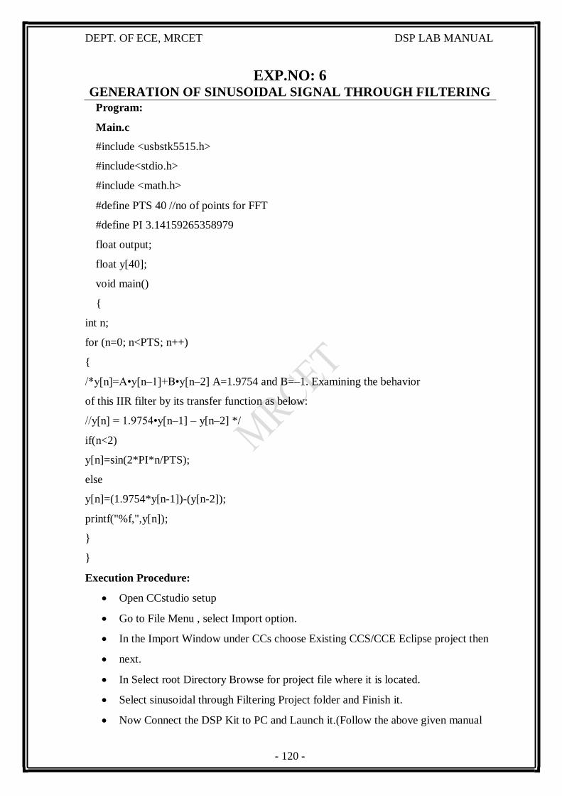
- 120 -
DEPT. OF ECE, MRCET DSP LAB MANUAL
EXP.NO: 6 GENERATION OF SINUSOIDAL SIGNAL THROUGH FILTERING
Program:
Main.c
#include <usbstk5515.h>
#include<stdio.h>
#include <math.h>
#define PTS 40 //no of points for FFT
#define PI 3.14159265358979
float output;
float y[40];
void main()
{
int n;
for (n=0; n<PTS; n++)
{
/*y[n]=A•y[n–1]+B•y[n–2] A=1.9754 and B=–1. Examining the behavior
of this IIR filter by its transfer function as below:
//y[n] = 1.9754•y[n–1] – y[n–2] */
if(n<2)
y[n]=sin(2*PI*n/PTS);
else
y[n]=(1.9754*y[n-1])-(y[n-2]);
printf("%f,",y[n]);
}
}
Execution Procedure:
Open CCstudio setup
Go to File Menu , select Import option.
In the Import Window under CCs choose Existing CCS/CCE Eclipse project then
next.
In Select root Directory Browse for project file where it is located.
Select sinusoidal through Filtering Project folder and Finish it.
Now Connect the DSP Kit to PC and Launch it.(Follow the above given manual
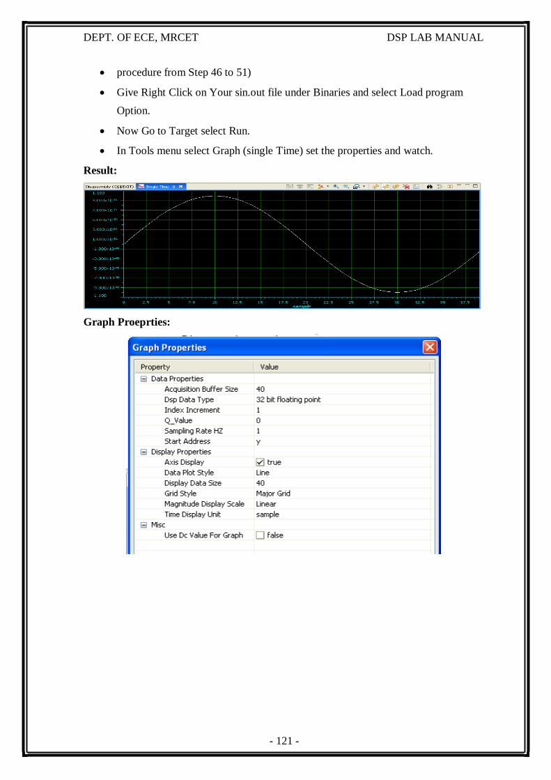
- 121 -
DEPT. OF ECE, MRCET DSP LAB MANUAL
procedure from Step 46 to 51)
Give Right Click on Your sin.out file under Binaries and select Load program
Option.
Now Go to Target select Run.
In Tools menu select Graph (single Time) set the properties and watch.
Result:
Graph Proeprties:

- 122 -
DEPT. OF ECE, MRCET DSP LAB MANUAL
OBSEVATIONS
Output Waveforms:
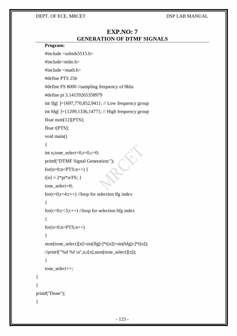
- 123 -
DEPT. OF ECE, MRCET DSP LAB MANUAL
EXP.NO: 7 GENERATION OF DTMF SIGNALS
Program:
#include <usbstk5515.h>
#include<stdio.h>
#include <math.h>
#define PTS 256
#define FS 8000 //sampling frequency of 8khz
#define pi 3.14159265358979
int lfg[ ]={697,770,852,941}; // Low frequency group
int hfg[ ]={1209,1336,1477}; // High frequency group
float num[12][PTS];
float t[PTS];
void main()
{
int n,tone_select=0,r=0,c=0;
printf("DTMF Signal Generation:");
for(n=0;n<PTS;n++) {
t[n] = 2*pi*n/FS; }
tone_select=0;
for(r=0;r<4;r++) //loop for selection lfg index
{
for(c=0;c<3;c++) //loop for selection hfg index
{
for(n=0;n<PTS;n++)
{
num[tone_select][n]=sin(lfg[r]*t[n])+sin(hfg[c]*t[n]);
//printf("%d %f \n",n,t[n],num[tone_select][n]);
}
tone_select++;
}
}
printf("Done");
}
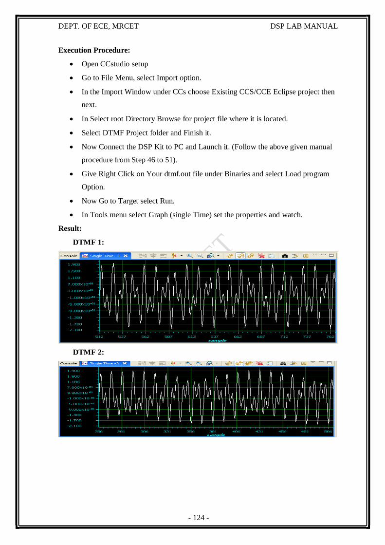
- 124 -
DEPT. OF ECE, MRCET DSP LAB MANUAL
Execution Procedure:
Open CCstudio setup
Go to File Menu, select Import option.
In the Import Window under CCs choose Existing CCS/CCE Eclipse project then
next.
In Select root Directory Browse for project file where it is located.
Select DTMF Project folder and Finish it.
Now Connect the DSP Kit to PC and Launch it. (Follow the above given manual
procedure from Step 46 to 51).
Give Right Click on Your dtmf.out file under Binaries and select Load program
Option.
Now Go to Target select Run.
In Tools menu select Graph (single Time) set the properties and watch.
Result:
DTMF 2:
DTMF 1:

- 125 -
DEPT. OF ECE, MRCET DSP LAB MANUAL
OBSEVATIONS
Output Waveforms:
- 126 -
DEPT. OF ECE, MRCET DSP LAB MANUAL
EXP.NO: 8 IMPLEMENTATION OF DECIMATION PROCESS
Program:
#include <usbstk5515.h>
#include<stdio.h>
#include <math.h>
#define PTS 256 //no of points for FFT
#define PI 3.14159265358979
float y1[PTS],y2[PTS],y3[PTS];
main()
{
int n,m;
printf("Enter Vaue for Decimation Factor\n");
scanf("%d",&m);
printf("Original signal samples:\n");
for(n=0;n<=PTS;n++) //original signal
{
y1[n]=sin(2*PI*10*(n)/(PTS));
printf("%d, %f\n",n,y1[n]);
}
printf("Decimated signal samples:\n");
for(n=0;n<=PTS;n++) //intrpol
{
y2[n]=sin(2*PI*10*n/(m*PTS));
printf("%d, %f\n",n,y2[n]);
}
} //end of main
Execution Procedure:
Open CCstudio setup
Go to File Menu, select Import option.
In the Import Window under CCs choose Existing CCS/CCE Eclipse project then
next.
In Select root Directory Browse for project file where it is located.
Select Decimation Project folder and Finish it.
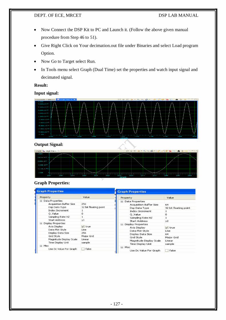
- 127 -
DEPT. OF ECE, MRCET DSP LAB MANUAL
Now Connect the DSP Kit to PC and Launch it. (Follow the above given manual
procedure from Step 46 to 51).
Give Right Click on Your decimation.out file under Binaries and select Load program
Option.
Now Go to Target select Run.
In Tools menu select Graph (Dual Time) set the properties and watch input signal and
decimated signal.
Result:
Input signal:
Graph Properties:
Output Signal:

- 128 -
DEPT. OF ECE, MRCET DSP LAB MANUAL
OBSEVATIONS
Output Waveforms:
- 129 -
DEPT. OF ECE, MRCET DSP LAB MANUAL
EXP.NO: 9
IMPLEMENTATION OF INTERPOLATION PROCESS
Program:
#include <usbstk5515.h>
#include<stdio.h>
#include <math.h>
#define PTS 256 //no of points for FFT
#define PI 3.14159265358979
float y1[PTS],y2[PTS],y3[PTS];
main()
{
int n,m;
printf("Enter Vaue for Interpolation Factor\n");
scanf("%d",&m);
printf("Original signal samples:\n");
for(n=0;n<=PTS;n++) //original signal
{
y1[n]=sin(2*PI*10*(n)/(PTS));
printf("%d, %f\n",n,y1[n]);
}
printf("Interpolated signal samples:\n");
for(n=0;n<=PTS;n++) //intrpol
{
y2[n]=sin(2*PI*10*(m*n)/(PTS));
printf("%d, %f\n",n,y2[n]);
}
}
Execution Procedure:
Open CCstudio setup
Go to File Menu, select Import option.
In the Import Window under CCs choose Existing CCS/CCE Eclipse project then
next.
In Select root Directory Browse for project file where it is located.
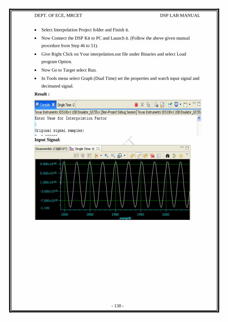
- 130 -
DEPT. OF ECE, MRCET DSP LAB MANUAL
Select Interpolation Project folder and Finish it.
Now Connect the DSP Kit to PC and Launch it. (Follow the above given manual
procedure from Step 46 to 51).
Give Right Click on Your interpolation.out file under Binaries and select Load
program Option.
Now Go to Target select Run.
In Tools menu select Graph (Dual Time) set the properties and watch input signal and
decimated signal.
Result :
Input Signal:
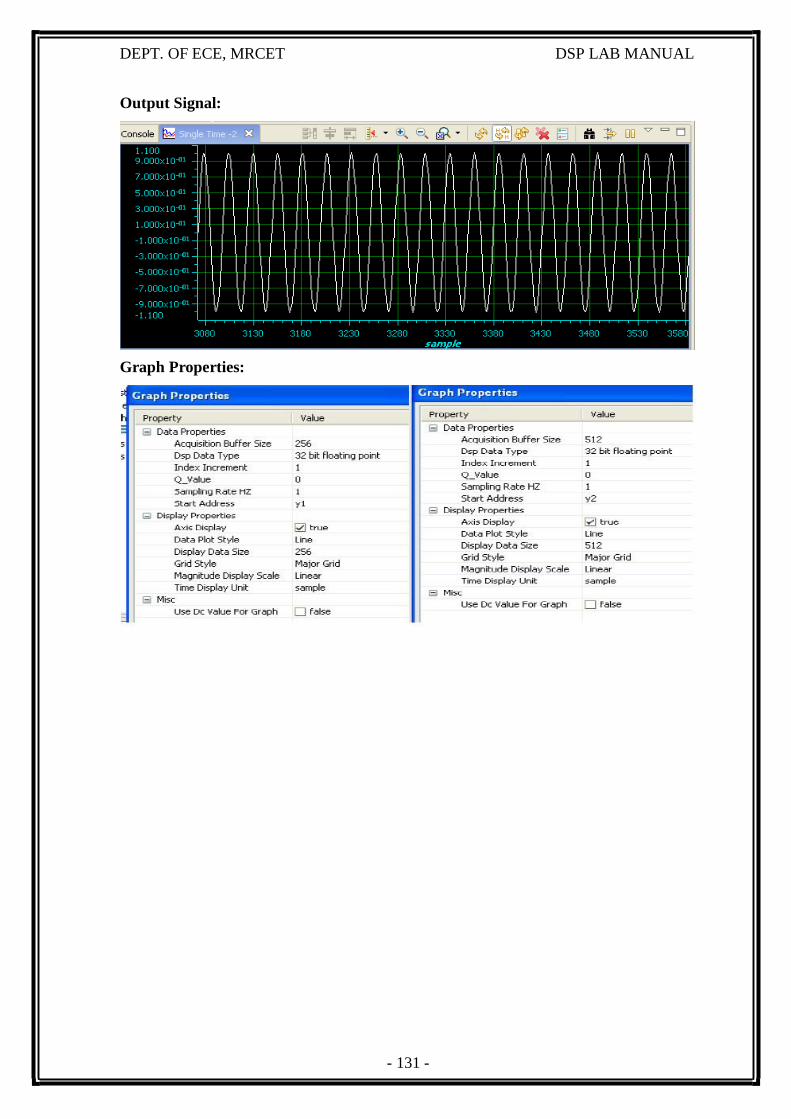
- 131 -
DEPT. OF ECE, MRCET DSP LAB MANUAL
Output Signal:
Graph Properties:

- 132 -
DEPT. OF ECE, MRCET DSP LAB MANUAL
OBSEVATIONS
Output Waveforms:
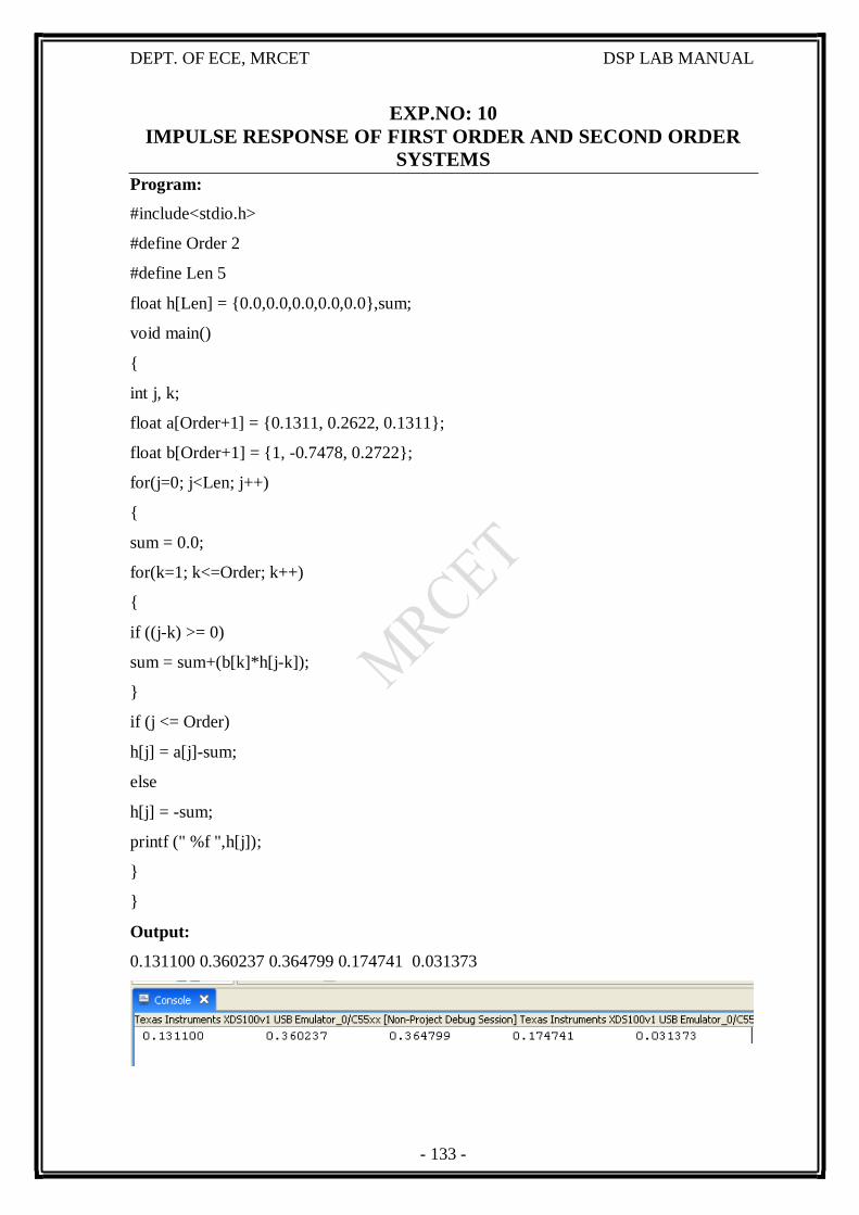
- 133 -
DEPT. OF ECE, MRCET DSP LAB MANUAL
EXP.NO: 10
IMPULSE RESPONSE OF FIRST ORDER AND SECOND ORDER
SYSTEMS
Program:
#include<stdio.h>
#define Order 2
#define Len 5
float h[Len] = {0.0,0.0,0.0,0.0,0.0},sum;
void main()
{
int j, k;
float a[Order+1] = {0.1311, 0.2622, 0.1311};
float b[Order+1] = {1, -0.7478, 0.2722};
for(j=0; j<Len; j++)
{
sum = 0.0;
for(k=1; k<=Order; k++)
{
if ((j-k) >= 0)
sum = sum+(b[k]*h[j-k]);
}
if (j <= Order)
h[j] = a[j]-sum;
else
h[j] = -sum;
printf (" %f ",h[j]);
}
}
Output:
0.131100 0.360237 0.364799 0.174741 0.031373
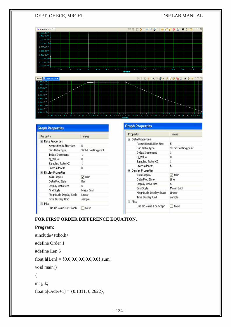
- 134 -
DEPT. OF ECE, MRCET DSP LAB MANUAL
FOR FIRST ORDER DIFFERENCE EQUATION.
Program:
#include<stdio.h>
#define Order 1
#define Len 5
float h[Len] = {0.0,0.0,0.0,0.0,0.0},sum;
void main()
{
int j, k;
float a[Order+1] = {0.1311, 0.2622};
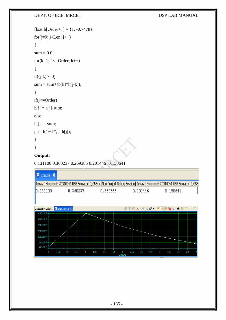
- 135 -
DEPT. OF ECE, MRCET DSP LAB MANUAL
float b[Order+1] = {1, -0.7478};
for(j=0; j<Len; j++)
{
sum = 0.0;
for(k=1; k<=Order; k++)
{
if((j-k)>=0)
sum = sum+(b[k]*h[j-k]);
}
if(j<=Order)
h[j] = a[j]-sum;
else
h[j] = -sum;
printf("%f ", j, h[j]);
}
}
Output:
0.131100 0.360237 0.269385 0.201446 0.150641
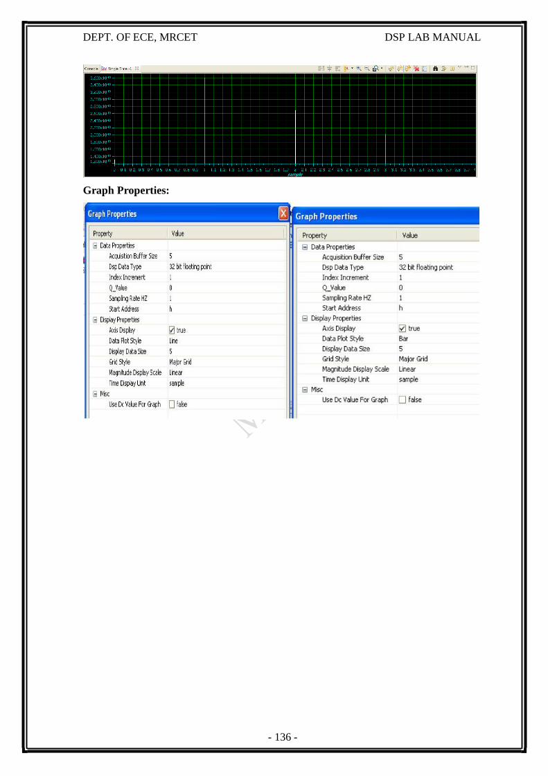
- 136 -
DEPT. OF ECE, MRCET DSP LAB MANUAL
Graph Properties:

- 137 -
DEPT. OF ECE, MRCET DSP LAB MANUAL
OBSEVATIONS
Output Waveforms:
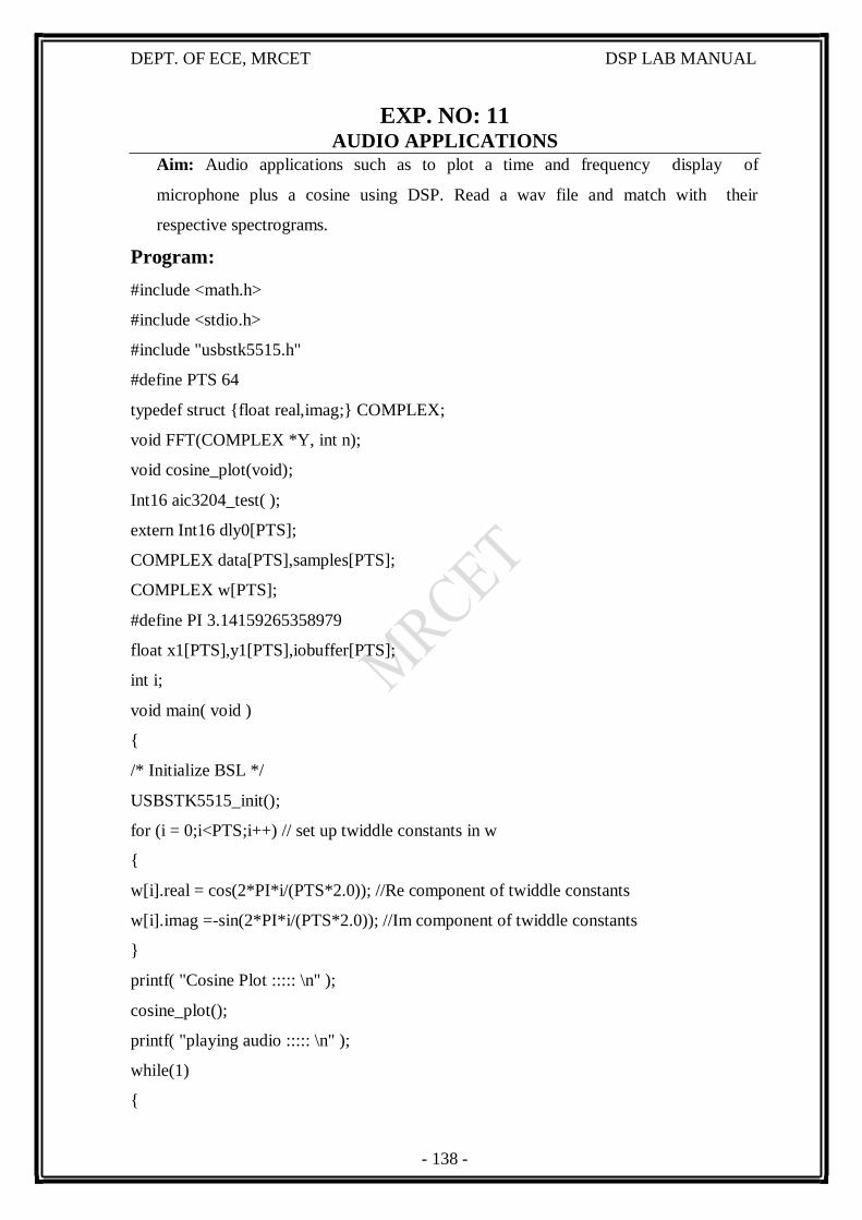
- 138 -
DEPT. OF ECE, MRCET DSP LAB MANUAL
EXP. NO: 11 AUDIO APPLICATIONS
Aim: Audio applications such as to plot a time and frequency display of
microphone plus a cosine using DSP. Read a wav file and match with their
respective spectrograms.
Program:
#include <math.h>
#include <stdio.h>
#include "usbstk5515.h"
#define PTS 64
typedef struct {float real,imag;} COMPLEX;
void FFT(COMPLEX *Y, int n);
void cosine_plot(void);
Int16 aic3204_test( );
extern Int16 dly0[PTS];
COMPLEX data[PTS],samples[PTS];
COMPLEX w[PTS];
#define PI 3.14159265358979
float x1[PTS],y1[PTS],iobuffer[PTS];
int i;
void main( void )
{
/* Initialize BSL */
USBSTK5515_init();
for (i = 0;i<PTS;i++) // set up twiddle constants in w
{
w[i].real = cos(2*PI*i/(PTS*2.0)); //Re component of twiddle constants
w[i].imag =-sin(2*PI*i/(PTS*2.0)); //Im component of twiddle constants
}
printf( "Cosine Plot ::::: \n" );
cosine_plot();
printf( "playing audio ::::: \n" );
while(1)
{
- 139 -
buffers
DEPT. OF ECE, MRCET DSP LAB MANUAL
aic3204_test( );
//for(i=0;i<PTS;i++)
// printf( "%d \n",dly0[i]);
for(i=0;i<PTS;i++)
{
data[i].real = dly0[i];
data[i].imag = 0.0;
}
FFT(data,PTS);
for (i = 0 ; i < PTS ; i++) //compute magnitude
{
x1[i] = sqrt(data[i].real*data[i].real + data[i].imag*data[i].imag);
printf("\n%d = %f",i,x1[i]);
}
}
}
void cosine_plot()
{
int i;
for (i = 0 ; i < PTS ; i++) //swap
{
iobuffer[i] = cos(2*PI*2*i/64.0);/*10- > freq, 64 -> sampling freq*/
printf("\n%d = %f",i,iobuffer[i]);
samples[i].real=0.0;
samples[i].imag=0.0;
}
for (i = 0 ; i < PTS ; i++) //swap buffers
{
samples[i].real=iobuffer[i]; //buffer with new data
}
for (i = 0 ; i < PTS ; i++)
samples[i].imag = 0.0; //imag components = 0
FFT(samples,PTS); //call function FFT.c
printf("\n output");
- 140 -
)
DEPT. OF ECE, MRCET DSP LAB MANUAL
for (i = 0 ; i < PTS ; i++) //compute magnitude
{
y1[i] = sqrt(samples[i].real*samples[i].real + samples[i].imag*samples[i].imag);
printf("\n%d = %f",i,x1[i]);
}
}
aic3204_loop_stereo_in1.C
#include "stdio.h"
#include "usbstk5515.h"
extern Int16 AIC3204_rset( Uint16 regnum, Uint16 regval);
#define Rcv 0x08
#define Xmit 0x20
#define N 64
Int16 data1, data2, data3, data4;
int sample,n,k,l;
Int16 dly0[N];
Int32 lyn,ryn;
Int16 aic3204_loop_stereo_in1(
{
// Int16 j, i = 0;
/* Configure AIC3204 */
AIC3204_rset( 0, 0 ); // Select page 0
AIC3204_rset( 1, 1 ); // Reset codec
AIC3204_rset( 0, 1 ); // Point to page 1
AIC3204_rset( 1, 8 ); // Disable crude AVDD generation from DVDD
AIC3204_rset( 2, 1 ); // Enable Analog Blocks, use LDO power
AIC3204_rset( 0, 0 ); // Select page 0
/* PLL and Clocks config and Power Up */
AIC3204_rset( 27, 0x0d ); // BCLK and WCLK is set as o/p to AIC3204(Master)
AIC3204_rset( 28, 0x00 ); // Data ofset = 0
AIC3204_rset( 4, 3 ); // PLL setting: PLLCLK <- MCLK, CODEC_CLKIN <-PLL CLK
AIC3204_rset( 6, 8 ); // PLL setting: J=8
AIC3204_rset( 7, 15 ); // PLL setting: HI_BYTE(D)
AIC3204_rset( 8, 0xdc ); // PLL setting: LO_BYTE(D)
- 141 -
DEPT. OF ECE, MRCET DSP LAB MANUAL
AIC3204_rset( 30, 0x88 ); // For 32 bit clocks per frame in Master mode ONLY
// BCLK=DAC_CLK/N =(12288000/8) = 1.536MHz = 32*fs
AIC3204_rset( 5, 0x91 ); // PLL setting: Power up PLL, P=1 and R=1
AIC3204_rset( 13, 0 );// Hi_Byte(DOSR) for DOSR = 128 decimal or 0x0080 DAC
oversamppling
AIC3204_rset( 14, 0x80 ); // Lo_Byte(DOSR) for DOSR = 128 decimal or 0x0080
AIC3204_rset( 20, 0x80 ); // AOSR for AOSR = 128 decimal or 0x0080 for decimation
filters 1 to 6
AIC3204_rset( 11, 0x88 ); // Power up NDAC and set NDAC value to 8
AIC3204_rset( 12, 0x82 ); // Power up MDAC and set MDAC value to 2
AIC3204_rset( 18, 0x88 ); // Power up NADC and set NADC value to 8
AIC3204_rset( 19, 0x82 ); // Power up MADC and set MADC value to 2
/* DAC ROUTING and Power Up */
AIC3204_rset( 0, 0x01 ); // Select page 1
AIC3204_rset( 12, 0x08 ); // LDAC AFIR routed to HPL
AIC3204_rset( 13, 0x08 ); // RDAC AFIR routed to HPR
AIC3204_rset( 0, 0x00 ); // Select page 0
AIC3204_rset( 64, 0x02 ); // Left vol=right vol
AIC3204_rset( 65, 0x00 ); // Left DAC gain to 0dB VOL; Right tracks Left
AIC3204_rset( 63, 0xd4 ); // Power up left,right data paths and set channel
AIC3204_rset( 0, 0x01 ); // Select page 1
AIC3204_rset( 16, 0x06 ); // Unmute HPL , 6dB gain
AIC3204_rset( 17, 0x06 ); // Unmute HPR , 6dB gain
AIC3204_rset( 9, 0x30 ); // Power up HPL,HPR
AIC3204_rset( 0, 0x00 ); // Select page 0
USBSTK5515_wait( 500 ); // Wait
/* ADC ROUTING and Power Up */
AIC3204_rset( 0, 1 ); // Select page 1
AIC3204_rset( 0x34, 0x30 ); // STEREO 1 Jack
// IN2_L to LADC_P through 40 kohm
AIC3204_rset( 0x37, 0x30 ); // IN2_R to RADC_P through 40 kohmm
AIC3204_rset( 0x36, 3 ); // CM_1 (common mode) to LADC_M through 40 kohm
AIC3204_rset( 0x39, 0xc0 ); // CM_1 (common mode) to RADC_M through 40 kohm
AIC3204_rset( 0x3b, 0 ); // MIC_PGA_L unmute
- 142 -
DEPT. OF ECE, MRCET DSP LAB MANUAL
AIC3204_rset( 0x3c, 0 ); // MIC_PGA_R unmute
AIC3204_rset( 0, 0 ); // Select page 0
AIC3204_rset( 0x51, 0xc0 ); // Powerup Left and Right ADC
AIC3204_rset( 0x52, 0 ); // Unmute Left and Right ADC
AIC3204_rset( 0, 0 );
USBSTK5515_wait( 200 ); // Wait
/* I2S settings */
I2S0_SRGR = 0x0;
I2S0_CR = 0x8010; // 16-bit word, slave, enable I2C
I2S0_ICMR = 0x3f; // Enable interrupts
/* Play Tone */
for(l=0;l<N;l++)
dly0[l]=0;
for ( sample = 0; sample < N ; sample++ )
{
USBSTK5515_waitusec(25);
/* Read Digital audio input */
data3 = I2S0_W0_MSW_R; // 16 bit left channel received audio data
data1 = I2S0_W0_LSW_R;
data4 = I2S0_W1_MSW_R; // 16 bit right channel received audio data
data2 = I2S0_W1_LSW_R;
while((Rcv & I2S0_IR) == 0); // Wait for interrupt pending flag
// printf("data3.. %d \n",data3);
USBSTK5515_wait(5000);
dly0[sample] = data3;
/* Write Digital audio input */
I2S0_W0_MSW_W = data3; // 16 bit left channel transmit audio data
I2S0_W0_LSW_W = 0;
I2S0_W1_MSW_W = data3; // 16 bit right channel transmit audio data
I2S0_W1_LSW_W = 0;
while((Xmit & I2S0_IR) == 0); // Wait for interrupt pending flag
}
/* Disble I2S */
I2S0_CR = 0x00;
- 143 -
DEPT. OF ECE, MRCET DSP LAB MANUAL
return 0;
}
aic3204_test.c
#define AIC3204_I2C_ADDR 0x18
#include "usbstk5515.h"
#include "usbstk5515_gpio.h"
#include "usbstk5515_i2c.h"
#include "stdio.h"
extern Int16 aic3204_tone_headphone( );
extern Int16 aic3204_loop_stereo_in1( );
Int16 AIC3204_rget( Uint16 regnum, Uint16* regval )
{
Int16 retcode = 0;
Uint8 cmd[2];
cmd[0] = regnum & 0x007F; // 7-bit Register Address
cmd[1] = 0;
retcode |= USBSTK5515_I2C_write( AIC3204_I2C_ADDR, cmd, 1 );
retcode |= USBSTK5515_I2C_read( AIC3204_I2C_ADDR, cmd, 1 );
*regval = cmd[0];
USBSTK5515_wait( 10 );
return retcode;
}
Int16 AIC3204_rset( Uint16 regnum, Uint16 regval )
{
Uint8 cmd[2];
cmd[0] = regnum & 0x007F; // 7-bit Register Address
cmd[1] = regval; // 8-bit Register Data
return USBSTK5515_I2C_write( AIC3204_I2C_ADDR, cmd, 2 );
}
Int16 aic3204_test( )
{
SYS_EXBUSSEL = 0x6100; // Enable I2C bus
USBSTK5515_I2C_init( ); // Initialize I2C
USBSTK5515_wait( 100 ); // Wait
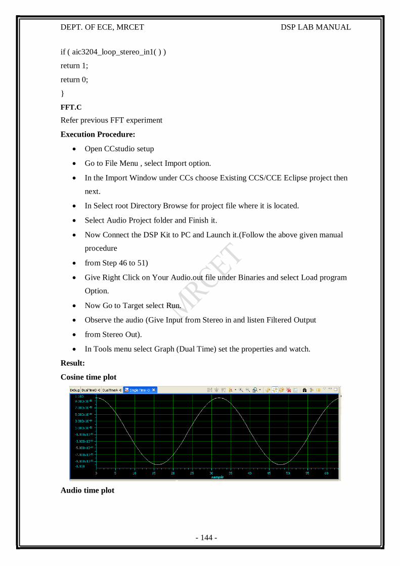
- 144 -
DEPT. OF ECE, MRCET DSP LAB MANUAL
if ( aic3204_loop_stereo_in1( ) )
return 1;
return 0;
}
FFT.C
Refer previous FFT experiment
Execution Procedure:
Open CCstudio setup
Go to File Menu , select Import option.
In the Import Window under CCs choose Existing CCS/CCE Eclipse project then
next.
In Select root Directory Browse for project file where it is located.
Select Audio Project folder and Finish it.
Now Connect the DSP Kit to PC and Launch it.(Follow the above given manual
procedure
from Step 46 to 51)
Give Right Click on Your Audio.out file under Binaries and select Load program
Option.
Now Go to Target select Run.
Observe the audio (Give Input from Stereo in and listen Filtered Output
from Stereo Out).
In Tools menu select Graph (Dual Time) set the properties and watch.
Result:
Cosine time plot
Audio time plot
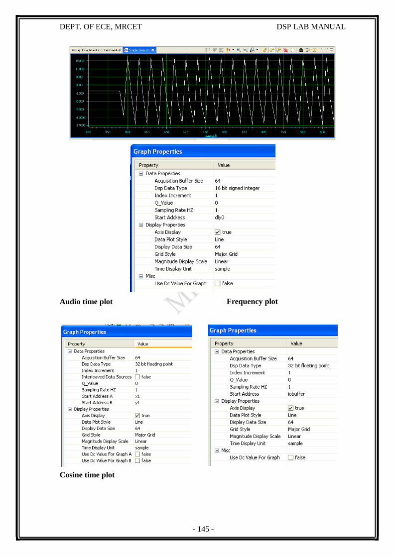
- 145 -
Frequency plot
DEPT. OF ECE, MRCET DSP LAB MANUAL
Audio time plot
Cosine time plot
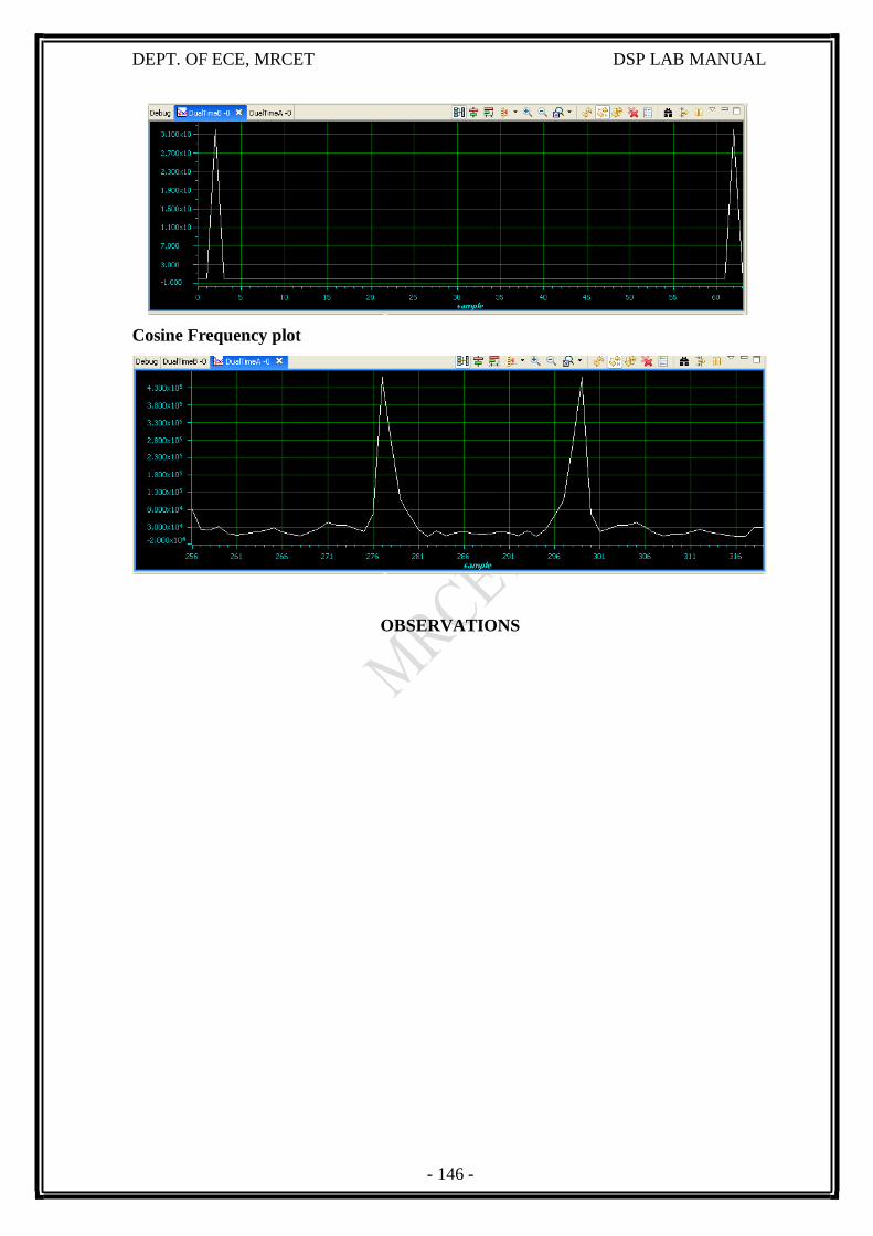
- 146 -
DEPT. OF ECE, MRCET DSP LAB MANUAL
Cosine Frequency plot
OBSERVATIONS
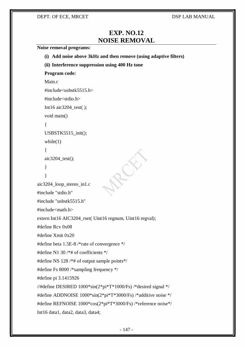
- 147 -
DEPT. OF ECE, MRCET DSP LAB MANUAL
Noise removal programs:
EXP. NO.12
NOISE REMOVAL
(i) Add noise above 3kHz and then remove (using adaptive filters)
(ii) Interference suppression using 400 Hz tone
Program code:
Main.c
#include<usbstk5515.h>
#include<stdio.h>
Int16 aic3204_test( );
void main()
{
USBSTK5515_init();
while(1)
{
aic3204_test();
}
}
aic3204_loop_stereo_in1.c
#include "stdio.h"
#include "usbstk5515.h"
#include<math.h>
extern Int16 AIC3204_rset( Uint16 regnum, Uint16 regval);
#define Rcv 0x08
#define Xmit 0x20
#define beta 1.5E-8 /*rate of convergence */
#define N1 30 /*# of coefficients */
#define NS 128 /*# of output sample points*/
#define Fs 8000 /*sampling frequency */
#define pi 3.1415926
//#define DESIRED 1000*sin(2*pi*T*1000/Fs) /*desired signal */
#define ADDNOISE 1000*sin(2*pi*T*3000/Fs) /*additive noise */
#define REFNOISE 1000*cos(2*pi*T*3000/Fs) /*reference noise*/
Int16 data1, data2, data3, data4;
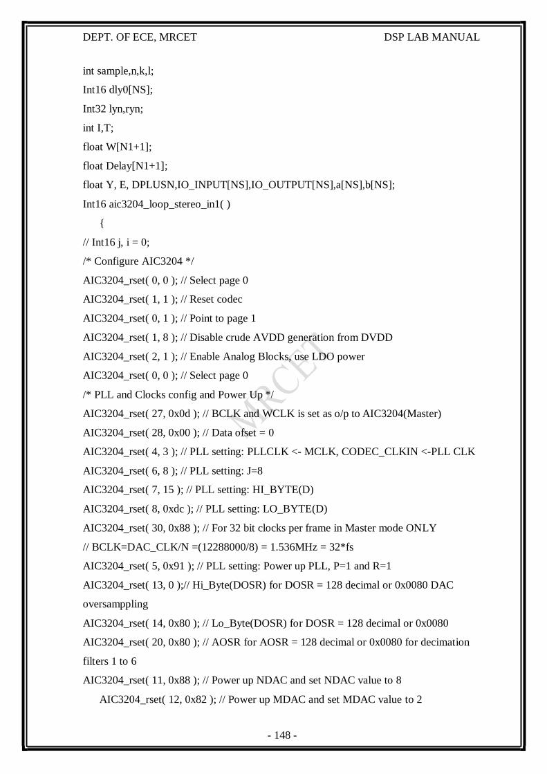
- 148 -
DEPT. OF ECE, MRCET DSP LAB MANUAL
int sample,n,k,l;
Int16 dly0[NS];
Int32 lyn,ryn;
int I,T;
float W[N1+1];
float Delay[N1+1];
float Y, E, DPLUSN,IO_INPUT[NS],IO_OUTPUT[NS],a[NS],b[NS];
Int16 aic3204_loop_stereo_in1( )
{
// Int16 j, i = 0;
/* Configure AIC3204 */
AIC3204_rset( 0, 0 ); // Select page 0
AIC3204_rset( 1, 1 ); // Reset codec
AIC3204_rset( 0, 1 ); // Point to page 1
AIC3204_rset( 1, 8 ); // Disable crude AVDD generation from DVDD
AIC3204_rset( 2, 1 ); // Enable Analog Blocks, use LDO power
AIC3204_rset( 0, 0 ); // Select page 0
/* PLL and Clocks config and Power Up */
AIC3204_rset( 27, 0x0d ); // BCLK and WCLK is set as o/p to AIC3204(Master)
AIC3204_rset( 28, 0x00 ); // Data ofset = 0
AIC3204_rset( 4, 3 ); // PLL setting: PLLCLK <- MCLK, CODEC_CLKIN <-PLL CLK
AIC3204_rset( 6, 8 ); // PLL setting: J=8
AIC3204_rset( 7, 15 ); // PLL setting: HI_BYTE(D)
AIC3204_rset( 8, 0xdc ); // PLL setting: LO_BYTE(D)
AIC3204_rset( 30, 0x88 ); // For 32 bit clocks per frame in Master mode ONLY
// BCLK=DAC_CLK/N =(12288000/8) = 1.536MHz = 32*fs
AIC3204_rset( 5, 0x91 ); // PLL setting: Power up PLL, P=1 and R=1
AIC3204_rset( 13, 0 );// Hi_Byte(DOSR) for DOSR = 128 decimal or 0x0080 DAC
oversamppling
AIC3204_rset( 14, 0x80 ); // Lo_Byte(DOSR) for DOSR = 128 decimal or 0x0080
AIC3204_rset( 20, 0x80 ); // AOSR for AOSR = 128 decimal or 0x0080 for decimation
filters 1 to 6
AIC3204_rset( 11, 0x88 ); // Power up NDAC and set NDAC value to 8
AIC3204_rset( 12, 0x82 ); // Power up MDAC and set MDAC value to 2
- 149 -
DEPT. OF ECE, MRCET DSP LAB MANUAL
AIC3204_rset( 18, 0x88 ); // Power up NADC and set NADC value to 8
AIC3204_rset( 19, 0x82 ); // Power up MADC and set MADC value to 2
/* DAC ROUTING and Power Up */
AIC3204_rset( 0, 0x01 ); // Select page 1
AIC3204_rset( 12, 0x08 ); // LDAC AFIR routed to HPL
AIC3204_rset( 13, 0x08 ); // RDAC AFIR routed to HPR
AIC3204_rset( 0, 0x00 ); // Select page 0
AIC3204_rset( 64, 0x02 ); // Left vol=right vol
AIC3204_rset( 65, 0x00 ); // Left DAC gain to 0dB VOL; Right tracks Left
AIC3204_rset( 63, 0xd4 ); // Power up left,right data paths and set channel
AIC3204_rset( 0, 0x01 ); // Select page 1
AIC3204_rset( 16, 0x06 ); // Unmute HPL , 6dB gain
AIC3204_rset( 17, 0x06 ); // Unmute HPR , 6dB gain
AIC3204_rset( 9, 0x30 ); // Power up HPL,HPR
AIC3204_rset( 0, 0x00 ); // Select page 0
USBSTK5515_wait( 500 ); // Wait
/* ADC ROUTING and Power Up */
AIC3204_rset( 0, 1 ); // Select page 1
AIC3204_rset( 0x34, 0x30 ); // STEREO 1 Jack
// IN2_L to LADC_P through 40 kohm
AIC3204_rset( 0x37, 0x30 ); // IN2_R to RADC_P through 40 kohmm
AIC3204_rset( 0x36, 3 ); // CM_1 (common mode) to LADC_M through 40 kohm
AIC3204_rset( 0x39, 0xc0 ); // CM_1 (common mode) to RADC_M through 40 kohm
AIC3204_rset( 0x3b, 0 ); // MIC_PGA_L unmute
AIC3204_rset( 0x3c, 0 ); // MIC_PGA_R unmute
AIC3204_rset( 0, 0 ); // Select page 0
AIC3204_rset( 0x51, 0xc0 ); // Powerup Left and Right ADC
AIC3204_rset( 0x52, 0 ); // Unmute Left and Right ADC
AIC3204_rset( 0, 0 );
USBSTK5515_wait( 200 ); // Wait
/* I2S settings */
I2S0_SRGR = 0x0;
I2S0_CR = 0x8010; // 16-bit word, slave, enable I2C
I2S0_ICMR = 0x3f; // Enable interrupts
- 150 -
DEPT. OF ECE, MRCET DSP LAB MANUAL
/* Play Tone */
for(l=0;l<NS;l++)
dly0[l]=0;
for(T=0;T<N1;T++)
{
W[T] = 0.0;
Delay[T] = 0.0;
}
for ( T = 0; T < NS ; T++ )
{ USBSTK5515_waitusec(25);
/* Read Digital audio input */
data3 = I2S0_W0_MSW_R; // 16 bit left channel received audio data
data1 = I2S0_W0_LSW_R;
data4 = I2S0_W1_MSW_R; // 16 bit right channel received audio data
data2 = I2S0_W1_LSW_R;
while((Rcv & I2S0_IR) == 0); // Wait for interrupt pending flag
// printf("data3.. %d \n",data3);
USBSTK5515_wait(5000);
dly0[T] = data3;
Delay[0] = REFNOISE; /*adaptive filter’s input*/
b[T]=DPLUSN = dly0[T]+ADDNOISE; /*desired + noise, d+n */
Y = 0;
for(I=0;I<N1;I++)
Y += (W[I] * Delay[I]); /*adaptive filter output */
E = DPLUSN-Y; /*error signal */
for(I=N1;I>0;I--)
{
W[I] = W[I]+(beta*E*Delay[I]); /*update weights */
if (I != 0)
Delay[I] = Delay[I-1]; /*update samples */
}
/* Write Digital audio input */
I2S0_W0_MSW_W = E; // 16 bit left channel transmit audio data
I2S0_W0_LSW_W = 0;
- 151 -
DEPT. OF ECE, MRCET DSP LAB MANUAL
I2S0_W1_MSW_W = E; // 16 bit right channel transmit audio data
I2S0_W1_LSW_W = 0;
while((Xmit & I2S0_IR) == 0); // Wait for interrupt pending flag
}
/* Disble I2S */
I2S0_CR = 0x00;
return 0;
}
/*
void apply_noise()
{
for(T=0;T<NS;T++) //# of output samples
{
a[T] = dly0[T];
IO_OUTPUT[T] = E; //overall output E
IO_INPUT[T]= DPLUSN; // store d + n
printf("%d %f %f\n",T,IO_INPUT[T],IO_OUTPUT[T]);
}
}*/
And one more .c file same as aic3204_test.c in the above experiment.
Execution Procedure:
Open CCstudio setup
Go to File Menu , select Import option.
In the Import Window under CCs choose Existing CCS/CCE Eclipse project then
next.
In Select root Directory Browse for project file where it is located.
Select FIR Project folder and Finish it.
Now Connect the DSP Kit to PC and Launch it.(Follow the above given manual
procedure
from Step 46 to 51)
Give Right Click on Your fir.out file under Binaries and select Load program
Option.
Now Go to Target select Run.
Observe the audio (Give Input from Stereo in and listen Filtered Output
from Stereo Out).

- 152 -
DEPT. OF ECE, MRCET DSP LAB MANUAL
OBSEVATIONS
Output Waveforms:
Related Documents


![EC1306 Digital Signal Processing Laboratory [REC]](https://static.cupdf.com/doc/110x72/5466b855b4af9fce288b4a87/ec1306-digital-signal-processing-laboratory-rec.jpg)