Welcome message from author
This document is posted to help you gain knowledge. Please leave a comment to let me know what you think about it! Share it to your friends and learn new things together.
Transcript

EE ��� Spring ����
DIGITAL VIDEO PROCESSING
A� Murat Tekalp
Department of Electrical Engineering� Hopeman ���University of Rochester� Rochester� New York �����
Ph� ��� �������� FAX� ��� ���� ��� E�mail� tekalp�ee�rochester�edu
The fundamentals of digital video representation� �ltering and compression� including pop�ular algorithms for ��D and ��D motion estimation� object tracking� frame rate conversion�deinterlacing� image enhancement� and the emerging international standards for image andvideo compression� with such applications as digital TV� web�based multimedia� videocon�ferencing� videophone and mobile image communications� Also included are more advancedimage compression techniques such as entropy coding� subband coding and object�basedcoding�
PART �� REPRESENTATION
Lecture � Introduction to Analog and Digital VideoLecture � Time�Varying Image Formation ModelsLecture � Spatio�Temporal SamplingLecture � Sampling Structure Conversion
PART �� MOTION ANALYSIS
Lecture � Optical Flow MethodsLecture � Block�Based MethodsLecture � Pel Recursive MethodsLecture � Bayesian MethodsLecture � Parametric Modeling and Motion SegmentationLecture � ��D Motion TrackingLecture �� ��D Motion and Structure EstimationLecture �� Stereo Video
PART �� FILTERING
Lecture �� Motion�Compensated FilteringLecture �� Standards ConversionLecture �� Noise FilteringLecture �� RestorationLecture �� Superresolution
�

PART �� STILL�IMAGE COMPRESSION
Lecture �� Fundamentals and Lossless CodingLecture �� DPCM and Transform CodingLecture � Still Image Compression StandardsLecture �� Subband�Wavelet Coding and Vector Quantization
PART �� VIDEO COMPRESSION
Lecture �� Interframe Compression MethodsLecture �� Frame�Based Video Compression StandardsLecture �� Object�Based Coding and MPEG��Lecture �� Digital Video Communication
Textbook�
Digital Video Processing� by A� Murat Tekalp� Prentice�Hall� �����
Supplementary Reading�
Video Engineering� by Inglis and Luther� Second Ed�� McGraw Hill� ����� covers funda�mentals of analog and digital video systems� including HDTV� CATV� terrestial and satellitevideo broadcast technologies�
Video Dialtone Technology� by Minoli� McGraw Hill� ����� covers digital video over ADSL�HFC� FTTC and ATM technologies� including interactive TV and video�on�demand�
Grading�
Homeworks ���Midterm Project ��� Written report due Mar� �Final Project � �To be presented May ���� Written report due May ��
Prerequisites�
EE ��� and EE ��� or EE ��� and permission of the instructor�
�

Digital Video Processing c�������� Prof� A� M� Tekalp��
��
LECTURE �
INTRODUCTION TO DIGITAL VIDEO
�� Analog Video
�� Digital Video
�� Digital Video Standards
� Digital Video Applications
� Digital TV
� PC Multimedia
� Real�time Communications
�� Digital Video Processing
c�������� This material is the property of A� M� Tekalp� It is intended for use only as a teaching aid when teaching
a regular semester or quarter based course at an academic institution using the textbook �Digital Video Processing�
�ISBN ���������� by A� M� Tekalp� Any other use of this material is strictly prohibited�
�

Digital Video Processing c�������� Prof� A� M� Tekalp��
��
ANALOG VIDEO
One or more analog signals that contain time�varying ��D intensity monochrome
or color� pattern and the timing information to align the pictures�
� Component Analog Video CAV�
� RGB
� YCrCb YIQ or YUV�
� Composite Video
� NTSC National Television Standards Committee�
� PAL Phase Alternating Line�
� SECAM SEquential Color And Memory�
� S�Video Y�C video�
� NTSC
� PAL
� SECAM
�

Digital Video Processing c�������� Prof� A� M� Tekalp��
��
Scanning and Frame�Rate
� Frame rate and �icker� Each complete picture is called a frame temporal
sampling�� Minimum frame rate required for icker�free viewing is �� Hz�
� Progressive scan� Each frame is made up of lines vertical sampling��
BC
A
D
C
A
B
FD
E
Raster scanning� a� progressive scan� b� interlaced scan�
� Interlaced scan� where each frame is split into two �elds� provides a tradeo�
between temporal and vertical resolution��
Digital Video Processing c�������� Prof� A� M� Tekalp��
��
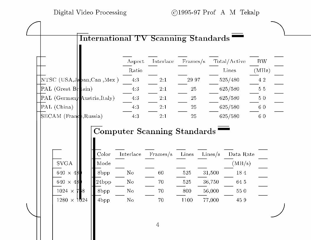
International TV Scanning Standards
Aspect Interlace Frames�s Total�Active BW
Ratio Lines �MHz�
NTSC �USA�Japan�Can��Mex�� ��� � ���� ���� ��
PAL �Great Britain� ��� � � � �� �
PAL �Germany�Austria�Italy� ��� � � � �� ��
PAL �China� ��� � � � �� ���
SECAM �France�Russia� ��� � � � �� ���
Computer Scanning Standards
Color Interlace Frames�s Lines Lines�s Data Rate
SVGA Mode �MB�s�
��� � ��� �bpp No �� �� �� ���
��� � ��� �bpp No �� ���� � ���
�� � ��� �bpp No �� ��� ����� ��
�� � �� �bpp No �� �� ������ � ��
Digital Video Processing c�������� Prof� A� M� Tekalp��
��
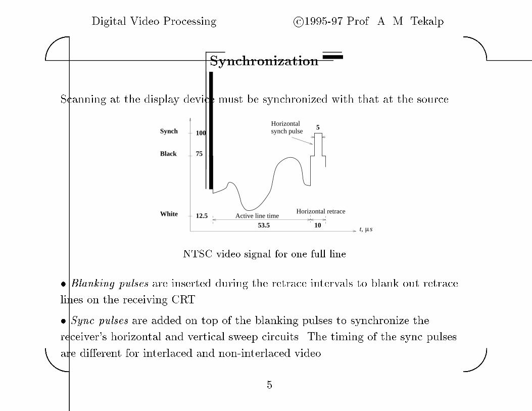
Synchronization
Scanning at the display device must be synchronized with that at the source�
1053.5
100
75
12.5
Synch
Black
White
5Horizontalsynch pulse
Active line time
µt, s
Horizontal retrace
NTSC video signal for one full line�
� Blanking pulses are inserted during the retrace intervals to blank out retrace
lines on the receiving CRT�
� Sync pulses are added on top of the blanking pulses to synchronize the
receiver�s horizontal and vertical sweep circuits� The timing of the sync pulses
are di�erent for interlaced and non�interlaced video�
�
Digital Video Processing c�������� Prof� A� M� Tekalp��
��
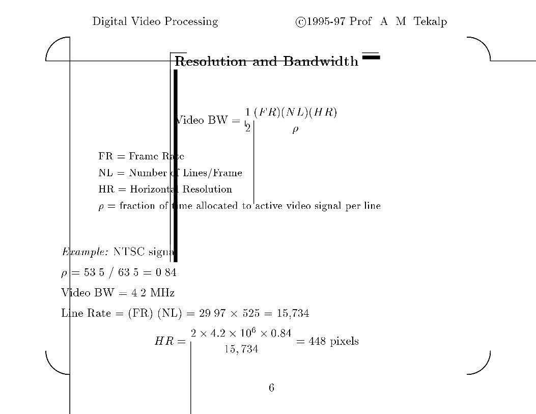
Resolution and Bandwidth
Video BW ��
�FR�NL�HR�
�
FR � Frame Rate
NL � Number of Lines�Frame
HR � Horizontal Resolution
� � fraction of time allocated to active video signal per line
Example� NTSC signal
� � ���� � ���� � ���
Video BW � �� MHz
Line Rate � FR� NL� � ����� � ��� � �����
HR ��� ��� ��� � ���
��� ��
� � pixels
�

Digital Video Processing c�������� Prof� A� M� Tekalp��
��
Spectral Content and Chrominance
v /L1
v /H2
F
Spectrum of the scanned video signal for still images�
0 1.25 5.75 64.83
4.2 MHz
6 MHz
sideband
picture color audio carrier carrier carrier
Spectrum of the NTSC video signal�
�

Digital Video Processing c�������� Prof� A� M� Tekalp��
��
Analog Video Acquisition
� Electronic CCD� video cameras � ITU�R standards ������ or ������
� recorded on video tape
� Motion picture cameras � � frames�s
� recorded on motion picture �lm
� Synthetic content � computer animation� graphics� etc�
� formed by sequential ordering of a set of still�frame images
Analog Video Recording
� Composite Video� VHS� U�matic
� Y�C Video� S�VHS
� CAV� Beta�cam
�

Digital Video Processing c�������� Prof� A� M� Tekalp��
��
DIGITAL REVOLUTION
� Digital data communications e�g�� computer networks� e�mail�
and� Digital audio e�g�� CD players� digital telephony�
What is next�
� Digital video � as a form of computer data
Products such as� digital TV�HDTV� videophone� multimedia PCs�
will be in the marketplace soon�
�� �Digital video�� IEEE Spectrum Magazine� pp� ����� Mar� ���
�

Digital Video Processing c�������� Prof� A� M� Tekalp��
��
What is the bottleneck for Digital Video�
Let�s look at the raw data rates for digital audio and video�
CD quality digital audio � kHz sampling rate x ��bits�sample
approximately ��� kbps
High de�nition video � ���� pels x ��� lines luma
�� pels x ��� lines chroma
x �� frames�s x � bits�pel�channel
approximately ����� Mbps
from the GA�HDTV proposal�
A picture is worth ���� words��
Inglis and Luther� Video Engineering� McGraw Hill� pp� ������ ����
��
Digital Video Processing c�������� Prof� A� M� Tekalp��
��
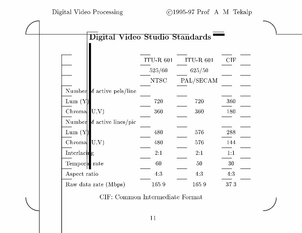
Digital Video Studio Standards
ITU�R � ITU�R � CIF
����� �����
NTSC PAL�SECAM
Number of active pels�line
Lum Y� �� �� ��
Chroma U�V� �� �� �
Number of active lines�pic
Lum Y� �� ��� ���
Chroma U�V� �� ��� ��
Interlacing �� �� �
Temporal rate � � �
Aspect ratio ��� ��� ���
Raw data rate Mbps� ���� ���� ����
CIF� Common Intermediate Format
��
Digital Video Processing c�������� Prof� A� M� Tekalp��
��
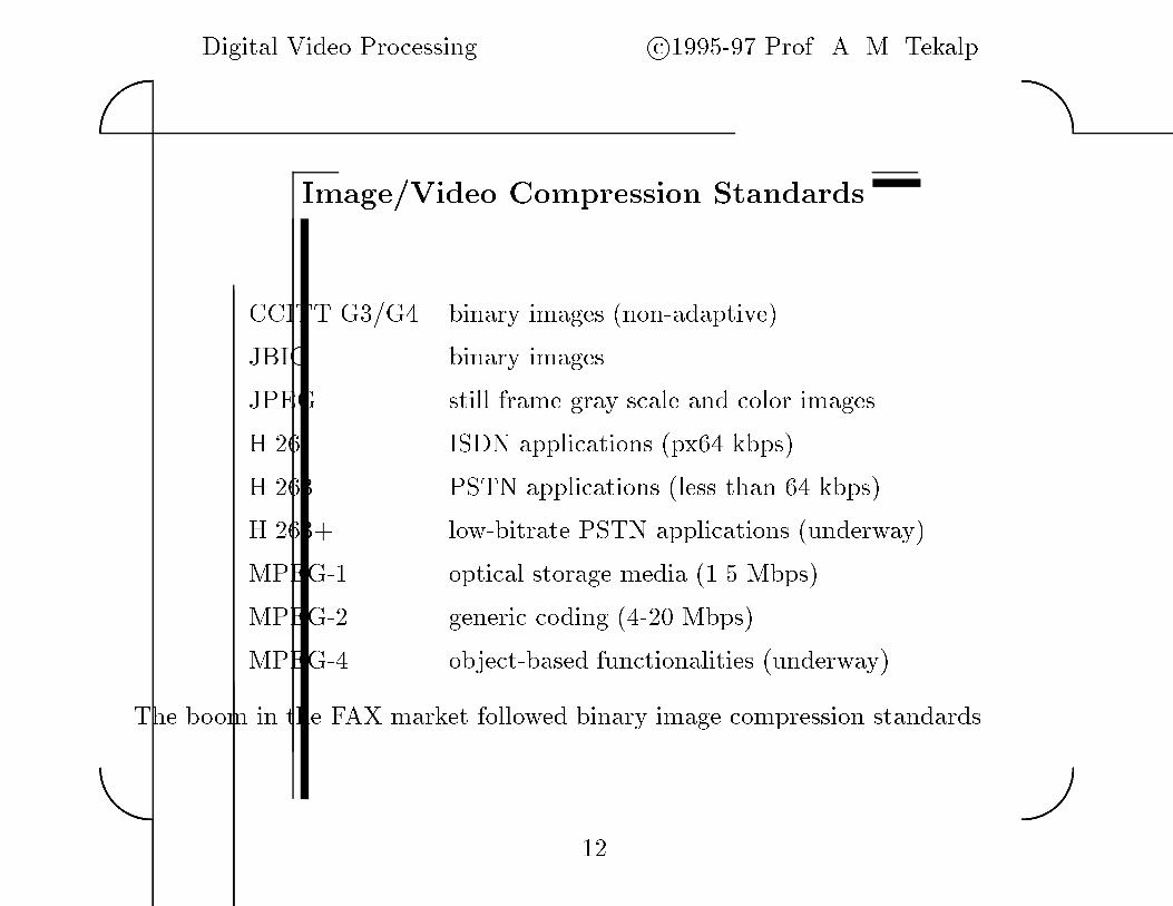
Image�Video Compression Standards
CCITT G��G binary images non�adaptive�
JBIG binary images
JPEG still frame gray scale and color images
H���� ISDN applications px� kbps�
H���� PSTN applications less than � kbps�
H����� low�bitrate PSTN applications underway�
MPEG�� optical storage media ��� Mbps�
MPEG�� generic coding ��� Mbps�
MPEG� object�based functionalities underway�
The boom in the FAX market followed binary image compression standards�
��
Digital Video Processing c�������� Prof� A� M� Tekalp��
��
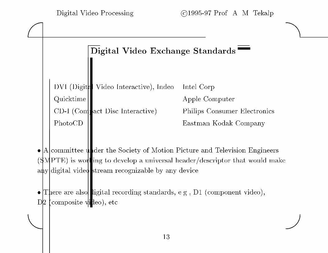
Digital Video Exchange Standards
DVI Digital Video Interactive�� Indeo Intel Corp�
Quicktime Apple Computer
CD�I Compact Disc Interactive� Philips Consumer Electronics
PhotoCD Eastman Kodak Company
� A committee under the Society of Motion Picture and Television Engineers
SMPTE� is working to develop a universal header�descriptor that would make
any digital video stream recognizable by any device�
� There are also digital recording standards� e�g�� D� component video��
D� composite video�� etc�
��
Digital Video Processing c�������� Prof� A� M� Tekalp��
��
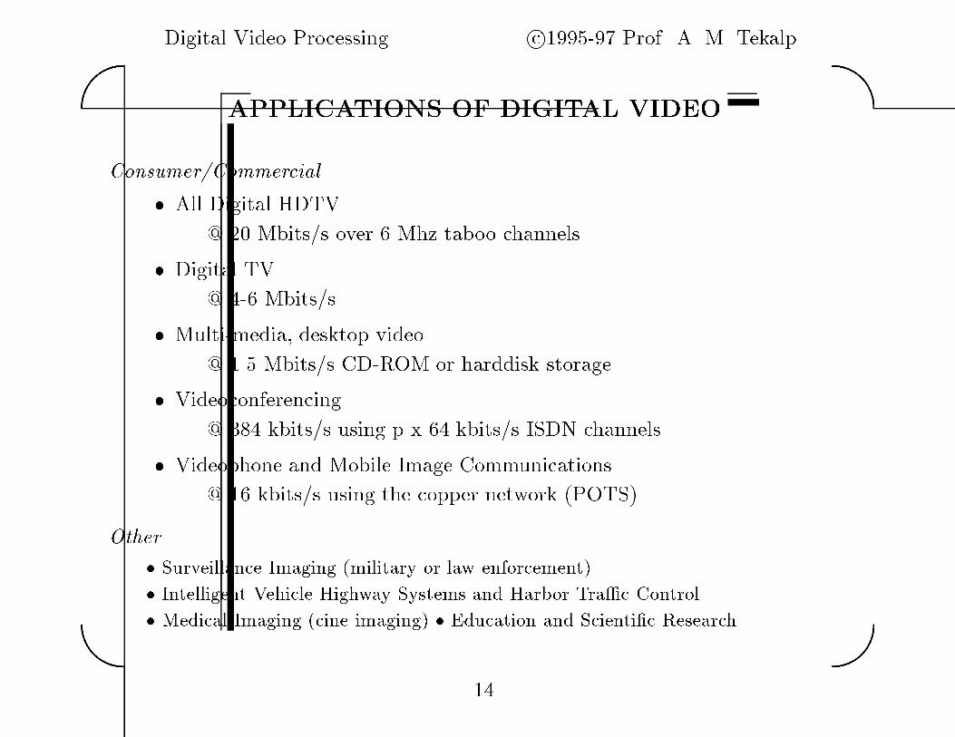
APPLICATIONS OF DIGITAL VIDEO
Consumer�Commercial
� All Digital HDTV
� �� Mbits�s over � Mhz taboo channels
� Digital TV
� �� Mbits�s
� Multi�media� desktop video
� ��� Mbits�s CD�ROM or harddisk storage
� Videoconferencing
� �� kbits�s using p x � kbits�s ISDN channels
� Videophone and Mobile Image Communications
� �� kbits�s using the copper network POTS�
Other� Surveillance Imaging military or law enforcement�
� Intelligent Vehicle Highway Systems and Harbor Tra�c Control
� Medical Imaging cine imaging� � Education and Scienti�c Research
�

Digital Video Processing c�������� Prof� A� M� Tekalp��
��
Digital TV
� Choices for ATV broadcast channels�
� terrestial broadcast
� direct satellite broadcast
� optical �ber cable broadcast
� Terrestial broadcast channels are � MHz in US and � MHz in Europe�
A � MHz channel can support about ����� Mbps data rate using
sophisticated modulation techniques e�g�� QAM or VSB��
� To broadcast digital HDTV over a ��MHz channel� we need about
����� � �� � � � � compression�
� A single ��MHz TV channel can support or � standard resolution
digital TV programs at �� Mbits�s each��
���Digital television�� IEEE Spectrum� April �� �
��

Digital Video Processing c�������� Prof� A� M� Tekalp��
��
PC Multimedia
� Early technologies
� Compact Disc�Interactive CD�I�
CD�based interactive full�screen� full�motion video
� Digital Video Interactive DVI� Technology
Hardware to handle full motion video in PCs at about ��� Mbit�s�
� VideoCD and Digital Video Disk DVD�
� Networked Multimedia � Video�on�Demand
�� �Special report� Interactive multimedia�� IEEE Spectrum� pp� ���� Mar� ����
�� J� van der Meer� �The full motion system for CD�I�� IEEE Trans� Cons� Electronics�
vol� ��� no� �� pp� ������ Nov� ���
��� J� Sutherland and L� Litteral� �Residential video services�� IEEE Comm� Mag��
pp� ����� July ���
��

Digital Video Processing c�������� Prof� A� M� Tekalp��
��
Real�Time Communications
� Digital Audio� The audio signal is sampled at � kHz and quantized with
���� bits�sample� Most telephony networks is capable to carry a load of
� kbps to �� kbps� Bit rate reduction is achieved by coarser quantization�
� Videoconferencing�videophone over ISDN� up to � Mbits�s using
H���� or H���� compression�
� Videophone over existing phone lines� � � �� kbits�s using H���� or
H����� compression�
� Video communications over future broadband ATM�access
networks�
� Constant Bit Rate CBR� channel � switched network
� Variable Bit Rate VBR� channel � quality of service contract
� Available Bit Rate ABR� channel � no guarantees� just like internet
��
Digital Video Processing c�������� Prof� A� M� Tekalp��
��
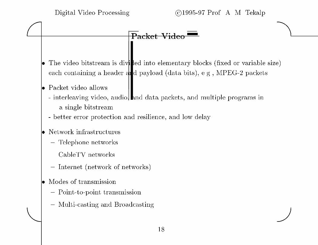
Packet Video
� The video bitstream is divided into elementary blocks �xed or variable size�
each containing a header and payload data bits�� e�g�� MPEG�� packets�
� Packet video allows
� interleaving video� audio� and data packets� and multiple programs in
a single bitstream
� better error protection and resilience� and low delay
� Network infrastructures
� Telephone networks
� CableTV networks
� Internet network of networks�
� Modes of transmission
� Point�to�point transmission
� Multi�casting and Broadcasting��

Digital Video Processing c�������� Prof� A� M� Tekalp��
��
Access Networks
� Fiber�to�Home
� Hybrid�Fiber�Coax Cable Modem�
� Fiber�to�Curb ADSL to home�
Some Access Network Bit�Rate Regimes
Conventional Telephone Modem ���� kbps
ISDN Integrated Services Digital Network� � � � kbps px��
T�� ��� Mbps
ADSL Asymmetric Digital Subscriber Line� ����� Mbps downstream
Cable Modem �� Mbps downstream
Ethernet packet�based LAN� �� Mbps
Fiber B�ISDN�ATM ������ Mbps
��
Digital Video Processing c�������� Prof� A� M� Tekalp��
��
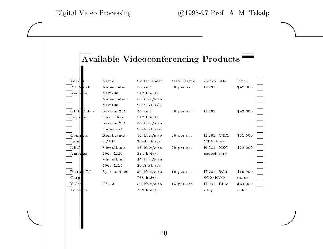
Available Videoconferencing Products
Vendor Name Codec speed Max Frame Comp� Alg� Price
BT North Videocodec �� and per sec H� �� �� �
America VC �� kbit�s
Videocodec �� kbit�s to
VC � �� kbit�s
GPT Video System �� �� and per sec H� �� �� �
Systems Twin chan� �� kbit�s
System �� �� kbit�s to
Universal �� kbit�s
Compres� Rembrandt �� kbit�s to per sec H� ��� CTX ����
Labs� II�VP �� kbit�s CTX Plus
NEC VisualLink �� kbit�s to per sec H� ��� NEC ���
America � M �� kbit�s proprietary
VisualLink �� kbit�s to
� M�� �� kbit�s
PictureTel System � �� kbit�s to � per sec H� ��� SG �����
Corp� ��� kbit�s SG �HVQ mono
Video CS� �� kbit�s to �� per sec H� ��� Blue �����
Telecom ��� kbit�s Chip color
��
Digital Video Processing c�������� Prof� A� M� Tekalp��
��
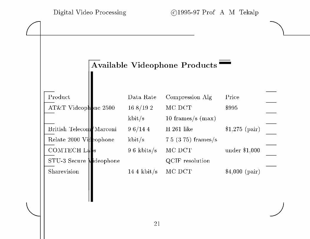
Available Videophone Products
Product Data Rate Compression Alg� Price
AT�T Videophone �� ������� MC DCT ����
kbit�s frames�s max�
British Telecom�Marconi ������� H��� like ����� pair�
Relate � Videophone kbit�s ��� ����� frames�s
COMTECH Labs� ��� kbits�s MC DCT under ���
STU�� Secure Videophone QCIF resolution
Sharevision ��� kbit�s MC DCT ��� pair�
��
Digital Video Processing c�������� Prof� A� M� Tekalp��
��
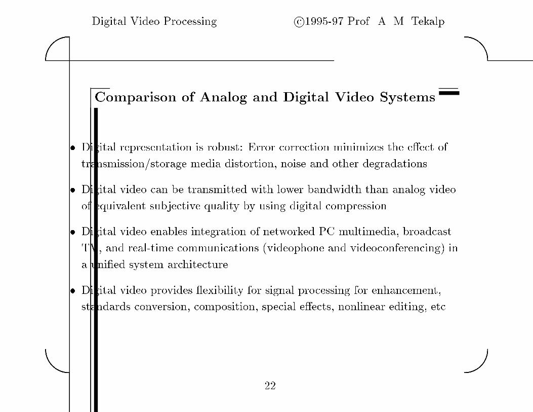
Comparison of Analog and Digital Video Systems
� Digital representation is robust� Error correction minimizes the e�ect of
transmission�storage media distortion� noise and other degradations�
� Digital video can be transmitted with lower bandwidth than analog video
of equivalent subjective quality by using digital compression�
� Digital video enables integration of networked PC multimedia� broadcast
TV� and real�time communications videophone and videoconferencing� in
a uni�ed system architecture�
� Digital video provides exibility for signal processing for enhancement�
standards conversion� composition� special e�ects� nonlinear editing� etc�
��
Digital Video Processing c�������� Prof� A� M� Tekalp��
��
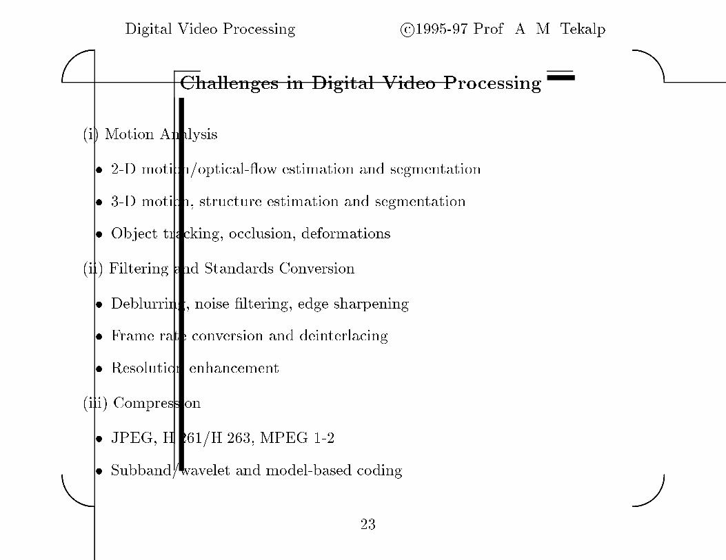
Challenges in Digital Video Processing
i� Motion Analysis
� ��D motion�optical� ow estimation and segmentation
� ��D motion� structure estimation and segmentation
� Object tracking� occlusion� deformations
ii� Filtering and Standards Conversion
� Deblurring� noise �ltering� edge sharpening
� Frame rate conversion and deinterlacing
� Resolution enhancement
iii� Compression
� JPEG� H�����H����� MPEG ���
� Subband�wavelet and model�based coding
��
Digital Video Processing c�������� Prof� A� M� Tekalp��
��
Di�erences Between Still�Frame and Video Processing
� Some tasks� such as motion estimation or the analysis of a time�varying
scene cannot be performed on the basis of a single image�
� Utilization of temporal redundancies that naturally exist in an image
sequence to develop e�ective algorithms�
� Motion�compensated �ltering
� Motion�compensated prediction�
Digital Video Processing c�������� Prof� A� M� Tekalp��
��
LECTURE ��
��D MOTION TRACKING
�� Token Tracking
�� Boundary Tracking
�� Object Tracking
� Single�Object Tracking
� Multiple�Object Tracking
� Object�Based Representation
Layering� Alpha�Plane� Mosaicing� etc��
���

Digital Video Processing c�������� Prof� A� M� Tekalp��
��
TOKEN TRACKING
� ��D Trajectory Model� Describe temporal evolution of selected feature
points� e�g��x�k �� � x�k� cos�k� � x�k� sin�k� t�k�
x�k �� � x�k� sin�k� x�k� cos�k� t�k�
with a ��D rotation by the angle �k� and translation by t�k� and t�k��
� Observation Model� Determine a number of feature correspondences over
multiple frames� e�g�� by block matching�
� Batch or Recursive Estimation�
Find the best motion parameters consistent with the model and
observations� Batch estimators� e�g�� the nonlinear least squares estimator�
process the entire data record at once after all data is collected� Recursive
estimators� e�g�� Kalman �lters� process each observation as it becomes
available to update the motion parameters�
���
Digital Video Processing c�������� Prof� A� M� Tekalp��
��
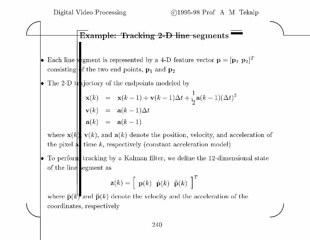
Example� Tracking ��D line segments
� Each line segment is represented by a �D feature vector p � �p� p��T
consisting of the two end points� p� and p��
� The ��D trajectory of the endpoints modeled by
xk� � xk � �� vk � ���t �
�ak � ���t��
vk� � ak � ���t
ak� � ak � ��
where xk�� vk�� and ak� denote the position� velocity� and acceleration of
the pixel at time k� respectively constant acceleration model��
� To perform tracking by a Kalman �lter� we de�ne the ���dimensional state
of the line segment aszk� �h
pk� �pk� �pk�iT
where �pk� and �pk� denote the velocity and the acceleration of the
coordinates� respectively�
��

Digital Video Processing c�������� Prof� A� M� Tekalp��
��
Example� �cont�d�
� The state propagation equation
zk� � �k� k � ��zk � �� wk�� k � �� � � � � N
where
�k� k � �� ��
���I� I��t ��I��t��
�� I� I��t
�� �� I�
����
and I� and �� are � identity and zero matrices� respectively�
wk� is a zero�mean� white process with the covariance matrix Qk��
� The observation equation
yk� � pk� vk�� k � �� � � � � N
It is assumed that the noisy observations can be estimated from pairs of
frames using some token�matching algorithm�
��

Digital Video Processing c�������� Prof� A� M� Tekalp��
��
BOUNDARY TRACKING
� Polygon tracking by tracking corners�
� Splines and active contours
�Propagate joint points by their motion vectors
�De�ne various energy functions to snap the propagated snake to
the contour in the next frame�
��
Digital Video Processing c�������� Prof� A� M� Tekalp��
��
OBJECT TRACKING
� Object�Based Editing � Synthetic Trans�guration
� Object�Based Coding � MPEG�
� Content�Based Retrieval � Digital Libraries
� ��D Object Modeling � Virtual Reality
��
Digital Video Processing c�������� Prof� A� M� Tekalp��
��
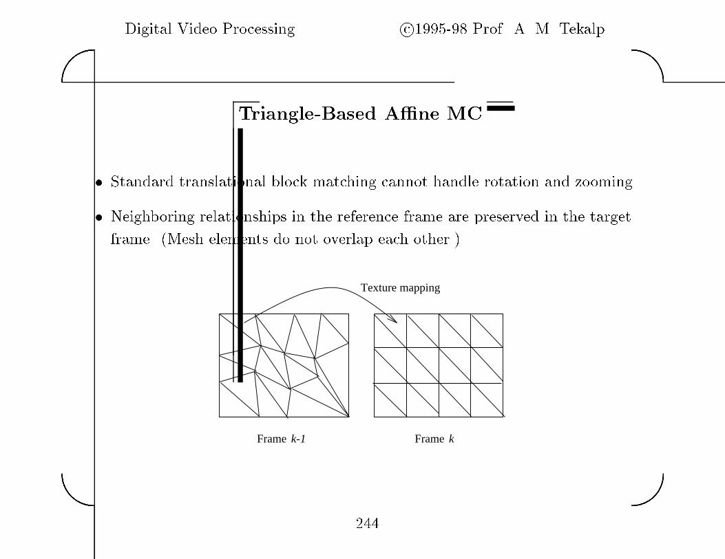
Triangle�Based Ane MC
� Standard translational block matching cannot handle rotation and zooming�
� Neighboring relationships in the reference frame are preserved in the target
frame� Mesh elements do not overlap each other��Frame k-1 Frame k
Texture mapping
�

Digital Video Processing c�������� Prof� A� M� Tekalp��
��
SINGLE OBJECT TRACKING
� ��D mesh based region tracking rather than token or boundary tracking�
� Projection of the mesh from frame to frame no temporal dynamic model�
� Mild deformations
� ��D mesh design regular� adaptive� or content�based�
� Object boundaries known
� Closed�form solutions and fast search for node motion re�nement
� Compensation of additive and multiplicative illumination di�erences
��

Digital Video Processing c�������� Prof� A� M� Tekalp��
��
��D Mesh Design
� Regular Mesh
Simple� no need to store node locations as part of the syntax�
Boundaries may not align with gray�level or motion edges�
� Adaptive Mesh
Split�merge re�nement of a regular mesh to align triangles with edges�
Split instructions can be easily incorporated into the syntax�
� Content�Based Mesh
Mesh optimized according to image content�
Costly� all node locations need to be stored�transmitted�
��
Digital Video Processing c�������� Prof� A� M� Tekalp��
��
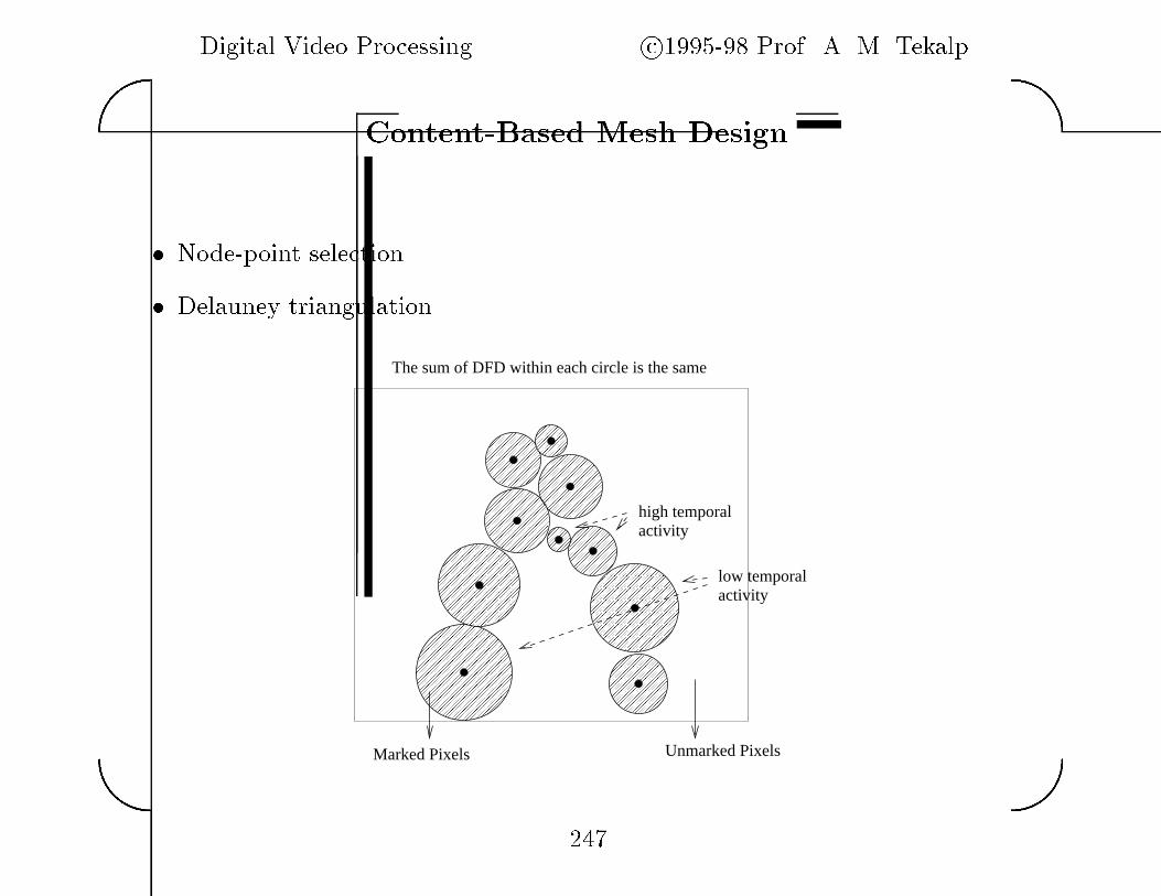
Content�Based Mesh Design
� Node�point selection
� Delauney triangulation
�������������������������
�������������������������
����������������
����������������
������������������������������������������
������������������������������������������
������������������������������������
������������������������������������
����������������������������������������������������������������
����������������������������������������������������������������
������������������������������
����������������������������������������������������������������������������������������������
����������������������������������������������������������������
�������������������������
�������������������������
������
������
��������������������������������������������������������
��������������������������������������������������������
Marked Pixels
The sum of DFD within each circle is the same
Unmarked Pixels
low temporalactivity
high temporalactivity
��

Digital Video Processing c�������� Prof� A� M� Tekalp��
��
Node�Point Selection
� Estimate ��D forward dense motion� �nd and polygonize the BTBC region�
Label all pixels within the BTBC polygon �marked�� and include its corners
in the list of node points�
� Compute the average DFD over the unmarked region�
� Compute a cost function Cx� y� over the unmarked region�
� Select the unmarked pixel with the highest Cx� y� which is not closer to any
of the existing node points by a prespeci�ed distance as the next node point�
� Grow a region about this node point until the sum of the absolute DFD
reaches a threshold� Label all points within this region as �marked��
� Continue until the maximum number of node points is reached� or all pixels
are �marked��
��

Digital Video Processing c�������� Prof� A� M� Tekalp��
��
Node�Point Motion Estimation
� Sampling from dense motion �eld
� Logarithmic hexagonal search Hierarchical�
� Closed�form connectivity�preserving solutions
� Node�based Polygon Matching�
� Patch�based
x
��
Digital Video Processing c�������� Prof� A� M� Tekalp��
��
Closed�Form Polygon Matching
� All N sets of a�ne parameters should yield the same motion vector at the
center node�
� A�ne parameters of two neighboring patches should yield the same motion
vectors along their common boundary line segment��
� Given at least N � correspondences within the hexagon� a linear least
squares solution can be found to determine all N sets of a�ne parameters�
� Given the spatio�temporal intensity gradients� a linear solution can be found
by constrained minimization Lagrange optimization��
���

Digital Video Processing c�������� Prof� A� M� Tekalp��
��
An Example� ��D Mesh Fitting
� Select a polygon enclosing the region of interest
� Overlay a ��D mesh e�g�� a uniform triangular mesh�
���

Digital Video Processing c�������� Prof� A� M� Tekalp��
��
Motion Estimation at the Boundary Nodes
Previous Frame
. . . . .
Reference Frame Current Frame
Assumption� Mild deformations
� De�ne a cost polygon about each boundary node
� Estimate the motion vector using deformable block matching
���
Digital Video Processing c�������� Prof� A� M� Tekalp��
��
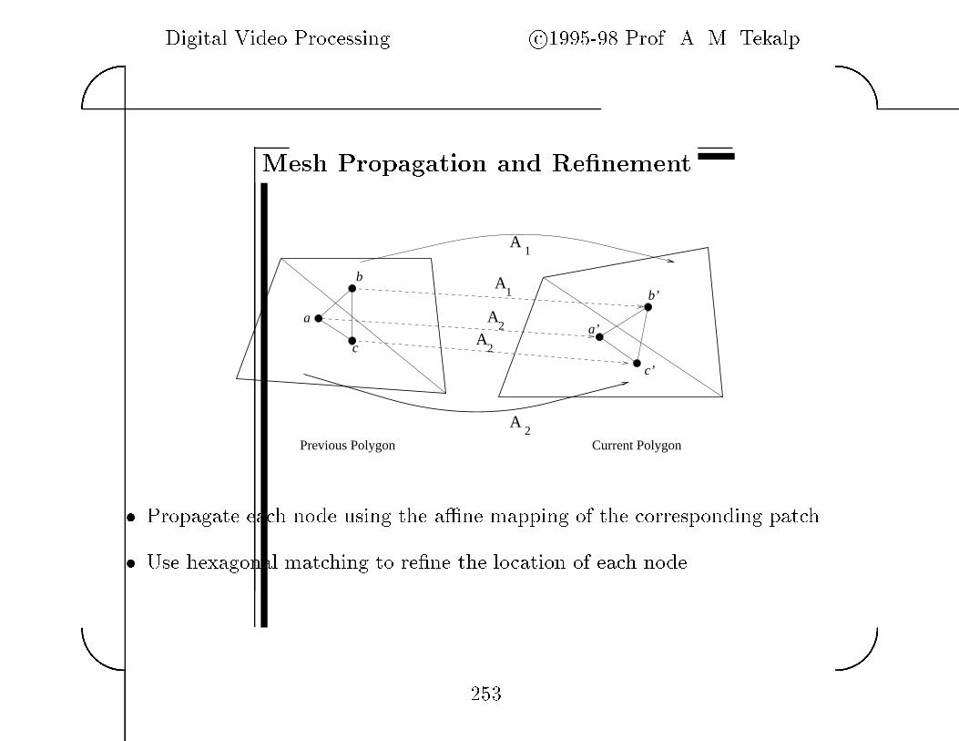
Mesh Propagation and Renement
A2
A2
A2
A1
Previous Polygon Current Polygon
A1
c
b
a
b’
c’
a’
� Propagate each node using the a�ne mapping of the corresponding patch
� Use hexagonal matching to re�ne the location of each node
���
Digital Video Processing c�������� Prof� A� M� Tekalp��
��
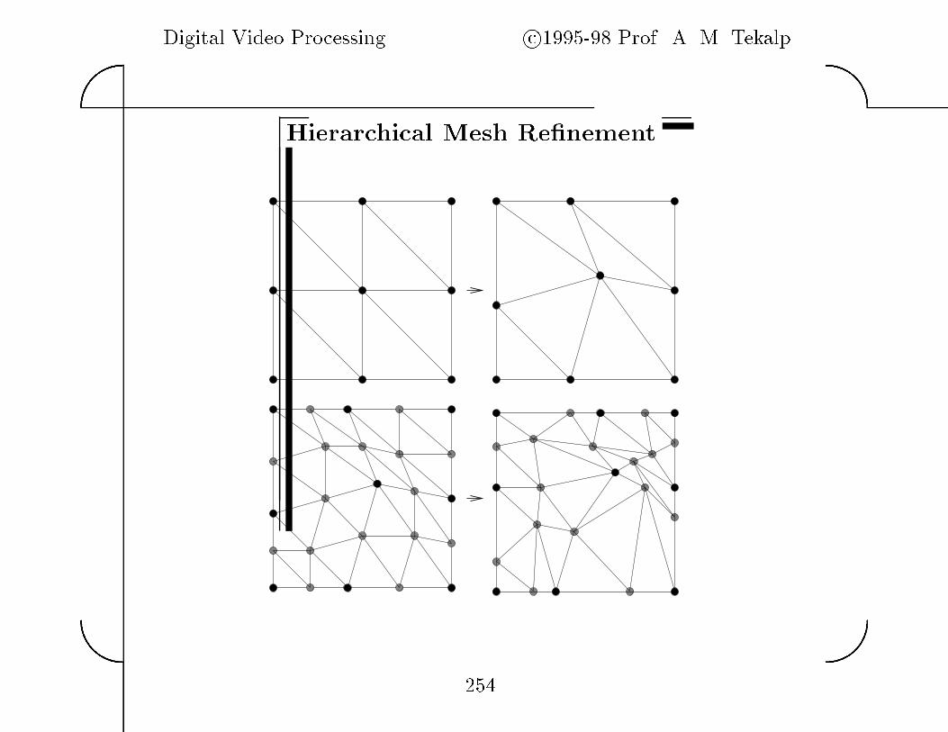
Hierarchical Mesh Renement
��
Digital Video Processing c�������� Prof� A� M� Tekalp��
��
Tracking Intensity Variations
Intensity Model�
Ix � �IR c
� scale factor
c intensity o�set
� Each node point is assigned a pair of parameters � and c
� Values of � and c at any x are bilinearly interpolated
���

Digital Video Processing c�������� Prof� A� M� Tekalp��
��
Select a polygon
bounding the ROI
Mesh fitting
Input video
Corner tracking
Mesh propagation
and refinement
Modified mesh
Image synthesis
Go to nextframe
Reference still image
Synthesized video
���

Digital Video Processing c�������� Prof� A� M� Tekalp��
��
MULTIPLE OBJECT TRACKING
� Occlusion�adaptive mesh modeling and design
� Motion estimation around object boundaries
� Interactions of multiple objects
� Temporary occlusions of objects
� Birth and death of objects
���
Digital Video Processing c�������� Prof� A� M� Tekalp��
��
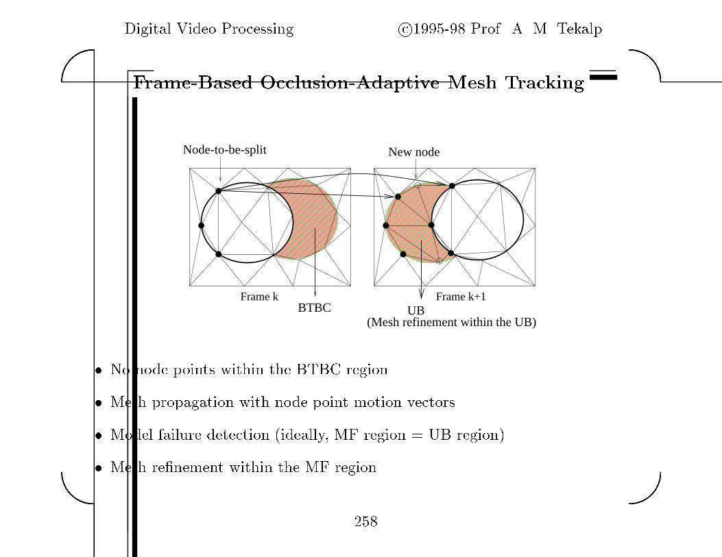
Frame�Based Occlusion�Adaptive Mesh Tracking
���������������������������������������������������������������������������������������������������
���������������������������������������������������������������������������������������������������
������������������������������������������������������������������������������������������������������������������������
������������������������������������������������������������������������������������������������������������������������
Frame k Frame k+1
New nodeNode-to-be-split
(Mesh refinement within the UB)UBBTBC
� No node points within the BTBC region
� Mesh propagation with node point motion vectors
� Model failure detection ideally� MF region � UB region�
� Mesh re�nement within the MF region���
Digital Video Processing c�������� Prof� A� M� Tekalp��
��
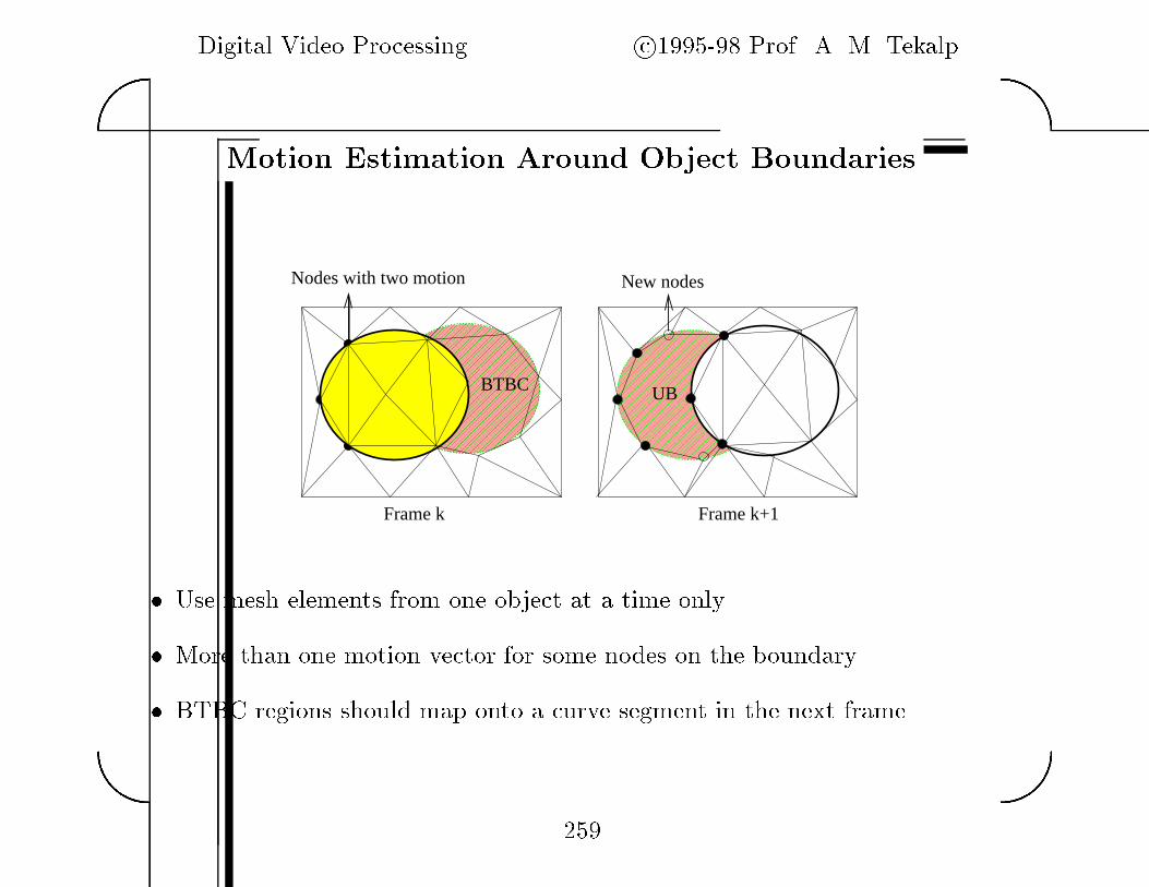
Motion Estimation Around Object Boundaries
���������������������������������������������������������������������������������������������������
���������������������������������������������������������������������������������������������������
��������������������������������������������������������������������������������������������������������������
��������������������������������������������������������������������������������������������������������������
���
���
���
���
���
���
���
���
���
���
�����
�����
�����
�����
�����
�����
�����
�����
�����
���������
����
����
����
����
����
����
����
����
����
Frame k Frame k+1
Nodes with two motion New nodes
BTBC UB
� Use mesh elements from one object at a time only
� More than one motion vector for some nodes on the boundary
� BTBC regions should map onto a curve segment in the next frame�
���
Digital Video Processing c�������� Prof� A� M� Tekalp��
��
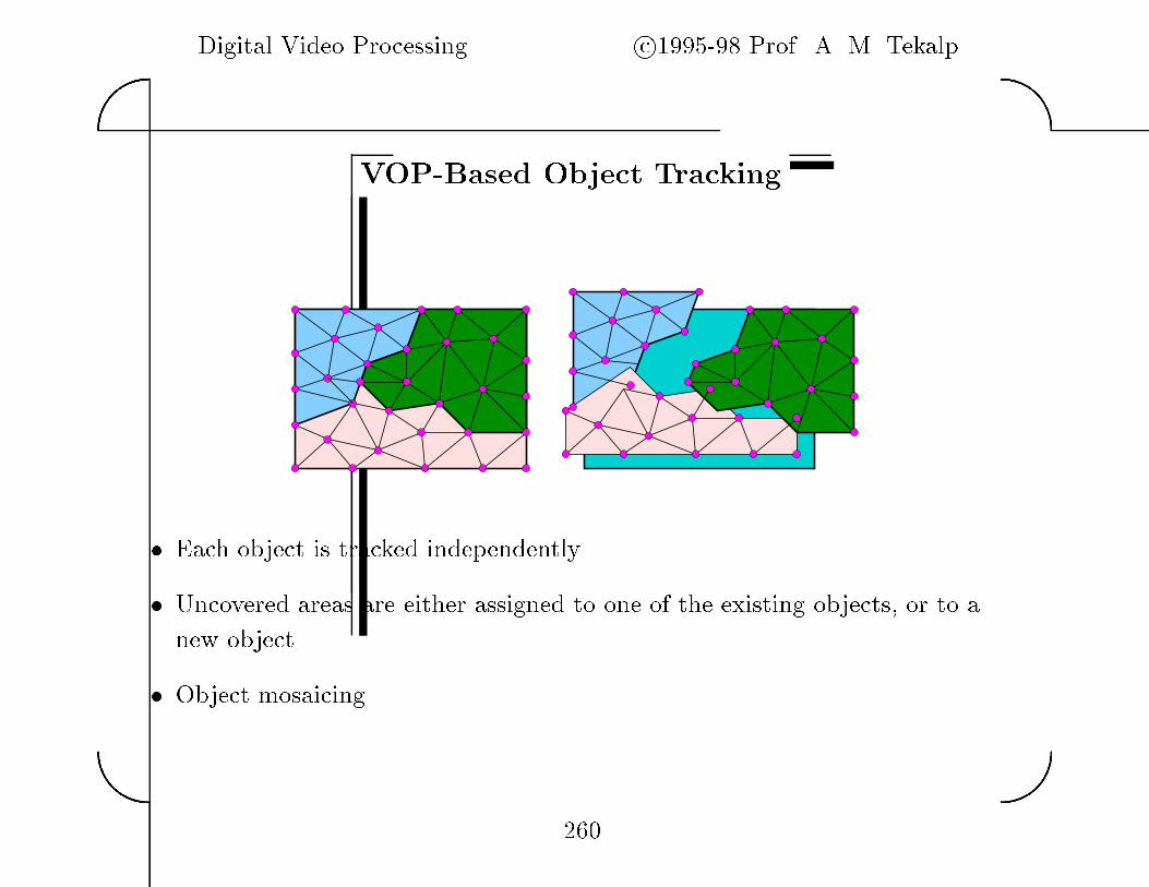
VOP�Based Object Tracking
� Each object is tracked independently�
� Uncovered areas are either assigned to one of the existing objects� or to a
new object�
� Object mosaicing�
���

Digital Video Processing c�������� Prof� A� M� Tekalp��
��
LECTURE �
TIME�VARYING IMAGE FORMATION MODELS
�� Video Source Model
�� Modeling ��D Rigid Motion
� ��D Translation Rotation and Scale
� Characterization of the Rotation Matrix
�� Homogeneous Coordinates
� Camera Models and Image Formation
� Projective Camera � Perspective Projection
� A�ne Camera � Weak�Perspective and Orthographic Projection
� Photometric Image Formation
c�������� This material is the property of A� M� Tekalp� It is intended for use only as a teaching aid when teaching
a regular semester or quarter based course at an academic institution using the textbook �Digital Video Processing�
�ISBN ���������� by A� M� Tekalp� Any other use of this material is strictly prohibited�
��

Digital Video Processing c�������� Prof� A� M� Tekalp��
��
VIDEO SOURCE MODEL
shot 1 shot N
� A video source is a collection of shots�
� A shot is a video clip recorded by an uninterrupted motion of a single camera�
� Shot boundaries can be clean �as in a camera break or blurred into a few
frames as in special e�ects such as dissolves wipes fade�ins and fade�outs�
��

Digital Video Processing c�������� Prof� A� M� Tekalp��
��
Source Modeling of a Video Shot
+3-D Scene Image Modeling Formation
ObservationNoise
SamplingSpatio-Temporal
Representation of digital video�
The variation in the intensity of the images from frame to frame is due to
� ��D camera motion e�g� zoom and pan etc�
� ��D object motion e�g� local translation and rotation
� photometric e�ects of ��D motion
� change in the scene illumination
We neglect deformable body motion at this time�
��
Digital Video Processing c�������� Prof� A� M� Tekalp��
��
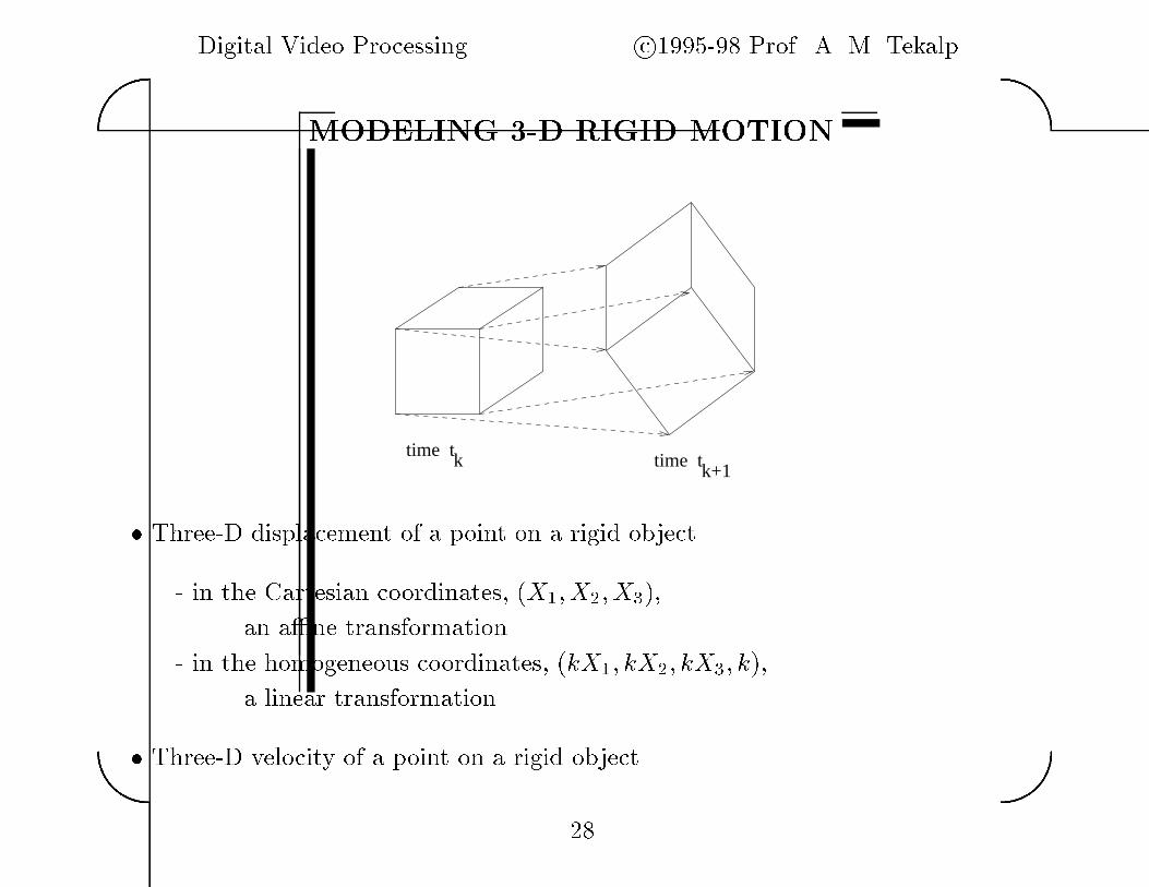
MODELING ��D RIGID MOTION
time tk time tk+1
� Three�D displacement of a point on a rigid object
� in the Cartesian coordinates �X�� X�� X�
an a�ne transformation
� in the homogeneous coordinates �kX�� kX�� kX�� k
a linear transformation
� Three�D velocity of a point on a rigid object
��
Digital Video Processing c�������� Prof� A� M� Tekalp��
��
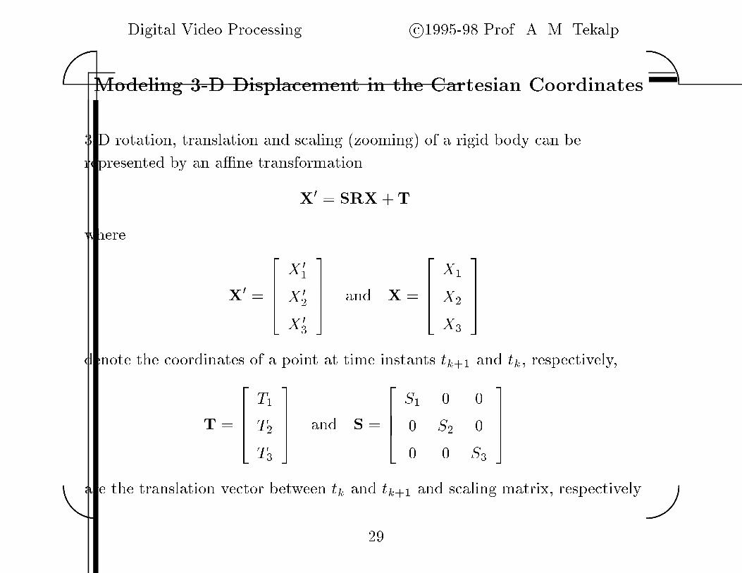
Modeling ��D Displacement in the Cartesian Coordinates
��D rotation translation and scaling �zooming of a rigid body can be
represented by an a�ne transformation
X
� � SRX�T
where
X
� ��
���X ��
X ��
X ��
���� and X �
����X�
X�
X�
����
denote the coordinates of a point at time instants tk�� and tk respectively
T ��
���T�
T�T�
���� and S �
����S� � �
� S� �
� � S��
���
are the translation vector between tk and tk�� and scaling matrix respectively�
��
Digital Video Processing c�������� Prof� A� M� Tekalp��
��
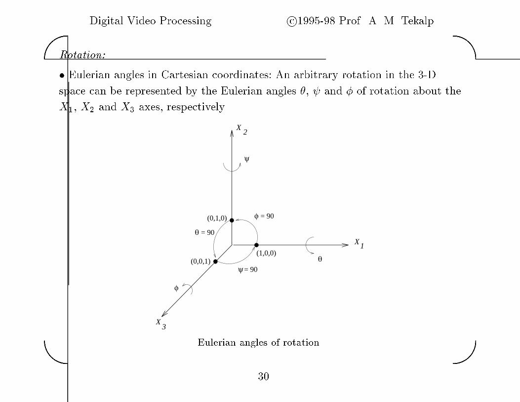
Rotation�
� Eulerian angles in Cartesian coordinates� An arbitrary rotation in the ��D
space can be represented by the Eulerian angles � � and � of rotation about the
X� X� and X� axes respectively�
ψ
φ
θ
φ
ψ= 90
= 90
θ = 90
(1,0,0)(0,0,1)
(0,1,0)
X
X
X
3
1
2
Eulerian angles of rotation�
��
Digital Video Processing c�������� Prof� A� M� Tekalp��
��
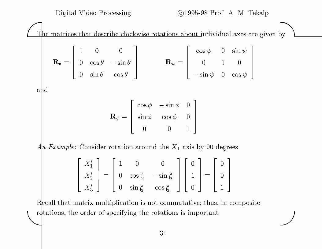
The matrices that describe clockwise rotations about individual axes are given by
R� ��
���� � �
� cos � � sin �
� sin � cos �
���� R� �
����cos� � sin�
� � �
� sin� � cos��
���
and
R� ��
���cos� � sin� �
sin� cos� �
� � ��
���
An Example� Consider rotation around the X� axis by �� degrees����X ��
X ��
X ��
���� �
����� � �
� cos ��
� sin ��
� sin ��
cos ��
����
�����
��
���� �
�����
��
����
Recall that matrix multiplication is not commutative� thus in composite
rotations the order of specifying the rotations is important�
��

Digital Video Processing c�������� Prof� A� M� Tekalp��
��
Assuming in�nitesmall rotation from frame to frame i�e� � � �� etc� and
approximating cos�� � � and sin�� � �� etc� these matrices simplify as
R� ��
���� � �
� � ���
� �� �
���� � R� �
����� � ��
� � �
��� � �
����
and
R� ��
���� ��� �
�� � �
� � ��
���
Then the composite rotation matrix R is given by�
R � R�R�R� ��
���� ��� ��
�� � ���
��� �� �
����
��

Digital Video Processing c�������� Prof� A� M� Tekalp��
��
� Rotation about an arbitrary axis in Cartesian coordinates�
A ��D rotation can be represented by an angle � about an axis described by the
directional cosines n� n� and n� through the origin�
α
X3
X2
X 1
(n , n , n )31 2
Rotation about an arbitrary axis�
��

Digital Video Processing c�������� Prof� A� M� Tekalp��
��
Then
R �
��� n
��
� ��� n�
��cos� n�n���� cos��� n�sin� n�n���� cos�� � n�sin�
n�n���� cos�� � n�sin� n�
�
� ��� n�
��cos� n�n���� cos�� � n�sin�
n�n���� cos��� n�sin� n�n���� cos�� � n�sin� n�
�
� ��� n�
��cos�
���
For an in�nitesmall solid angle �� R reduces to
R �
����� �n��� n���
n��� � �n���
�n��� n��� �
����
and we have
�� � n���
�� � n���
�� � n����
�

Digital Video Processing c�������� Prof� A� M� Tekalp��
��
Three�D Velocity Model
Start with the ��D displacement model for rotation and translation only�����X ��
X ��
X ��
���� �
����� ��� ��
�� � ���
��� �� �
����
����X�
X�
X�
�����
����T�
T�T�
����
lim�t��
����
X���X�
�t
X� �X
�t
X��X
�t
���� � lim�t��
���� �
���t
���t
���t
�
���t
�
���t
���t
����
����X�
X�
X�
����� lim�t��
����
T��t
T �t
T�t
����
����X�
X�X�
���� �
���� ��� ��
�� ���
��� ��
����
����X�
X�
X�
�����
����V�
V�V�
����
where �i and Vi denote the angular and translational velocities respectively�
for i � �� �� ��
��
Digital Video Processing c�������� Prof� A� M� Tekalp��
��
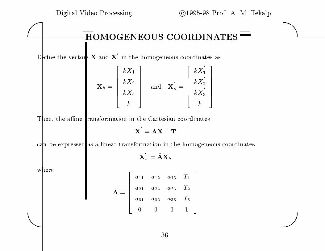
HOMOGENEOUS COORDINATES
De ne the vectors X and X�
in the homogeneous coordinates as
Xh ��
�����kX�
kX�
kX�
k
������ and X
�h �
������kX�
�
kX�
�
kX�
�
k
������
Then� the a�ne transformation in the Cartesian coordinates
X
�
� AX�T
can be expressed as a linear transformation in the homogeneous coordinates
X
�h � �AXh
where
�A ��
�����a�� a�� a�� T�
a�� a�� a�� T�
a�� a�� a�� T�
�
������
��

Digital Video Processing c�������� Prof� A� M� Tekalp��
��
Translation�
X
�h � �TXh
where
�T ��
������� � � T�
� � � T�
� � � T�
� � � ��
������
Scaling �Zooming��
X
�h � �SXh
where
�S ��
������S� � � �
� S� � �
� � S� �
� � � ��
������
��

Digital Video Processing c�������� Prof� A� M� Tekalp��
��
Rotation�
X
�h ��RXh
where
�R ��
������r�� r�� r�� �
r�� r�� r�� �
r�� r�� r�� �
� � � ��
������
rij denotes the elements of the rotation matrix in the Cartesian coordinates�
��
Digital Video Processing c�������� Prof� A� M� Tekalp��
��
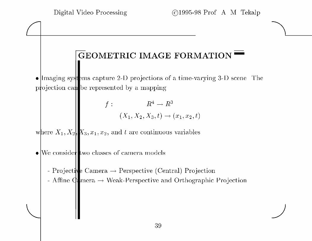
GEOMETRIC IMAGE FORMATION
� Imaging systems capture ��D projections of a time�varying ��D scene� The
projection can be represented by a mapping
f � R� � R�
�X�� X�� X�� t � �x�� x�� t
where X�� X�� X�� x�� x� and t are continuous variables�
� We consider two classes of camera models
� Projective Camera � Perspective �Central Projection
� A�ne Camera � Weak�Perspective and Orthographic Projection
��
Digital Video Processing c�������� Prof� A� M� Tekalp��
��
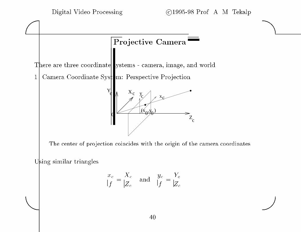
Projective Camera
There are three coordinate systems � camera image and world�
�� Camera Coordinate System� Perspective Projection
Yc
(x ,y )0 0Zc
Xc
O
xcyc
The center of projection coincides with the origin of the camera coordinates�
Using similar triangles
xcf�Xc
Zc
and
ycf�Yc
Zc
�

Digital Video Processing c�������� Prof� A� M� Tekalp��
��
Perspective projection is nonlinear in the Cartesian coordinates� however it can
be expressed as a linear operation in the homogeneous coordinates�
����xc
ycf
���� � �
����Xc
YcZc
���� � �
�����
�
� �
����
�����Xc
YcZc
�
������
where
� � f�Zc�
Digital Video Processing c�������� Prof� A� M� Tekalp��
��
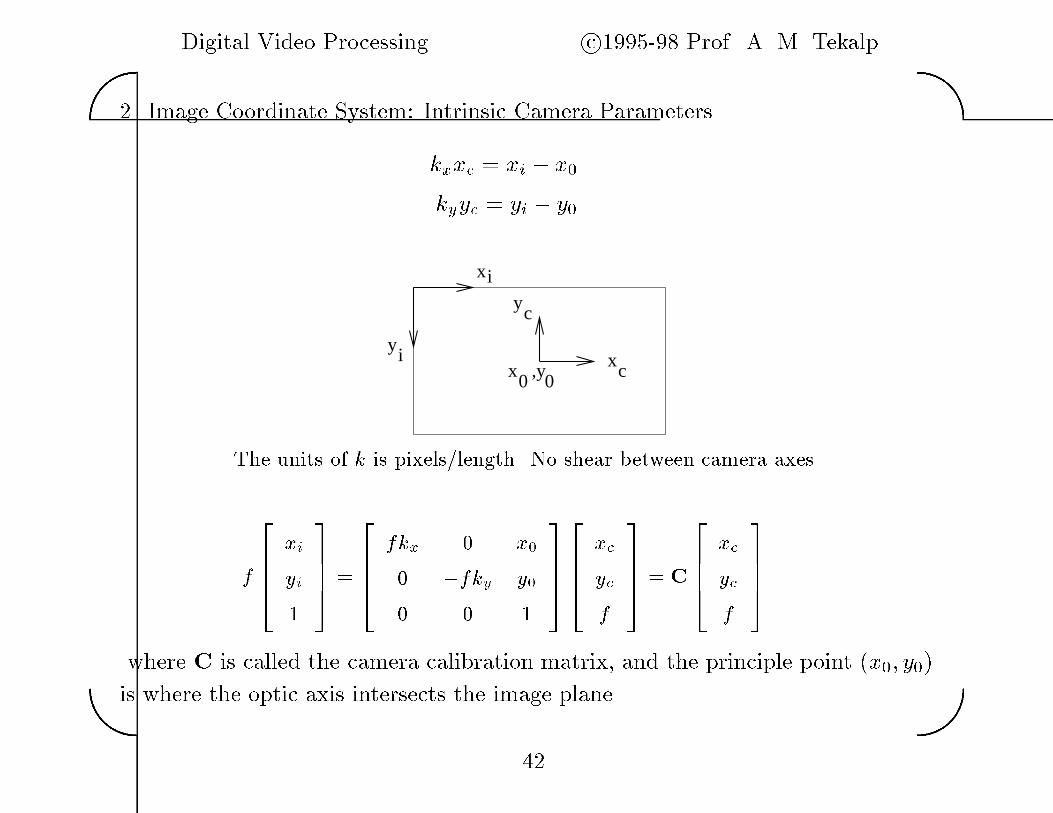
�� Image Coordinate System� Intrinsic Camera Parameters
kxxc � xi � x�
kyyc � yi � y�
xi
yi0x ,y0
xc
yc
The units of k is pixels�length� No shear between camera axes�
f�
���xi
yi�
���� �
����fkx x�
�fky y�
�
����
����xc
ycf
���� � C
����xc
ycf
����
where C is called the camera calibration matrix and the principle point �x�� y�
is where the optic axis intersects the image plane�
�
Digital Video Processing c�������� Prof� A� M� Tekalp��
��
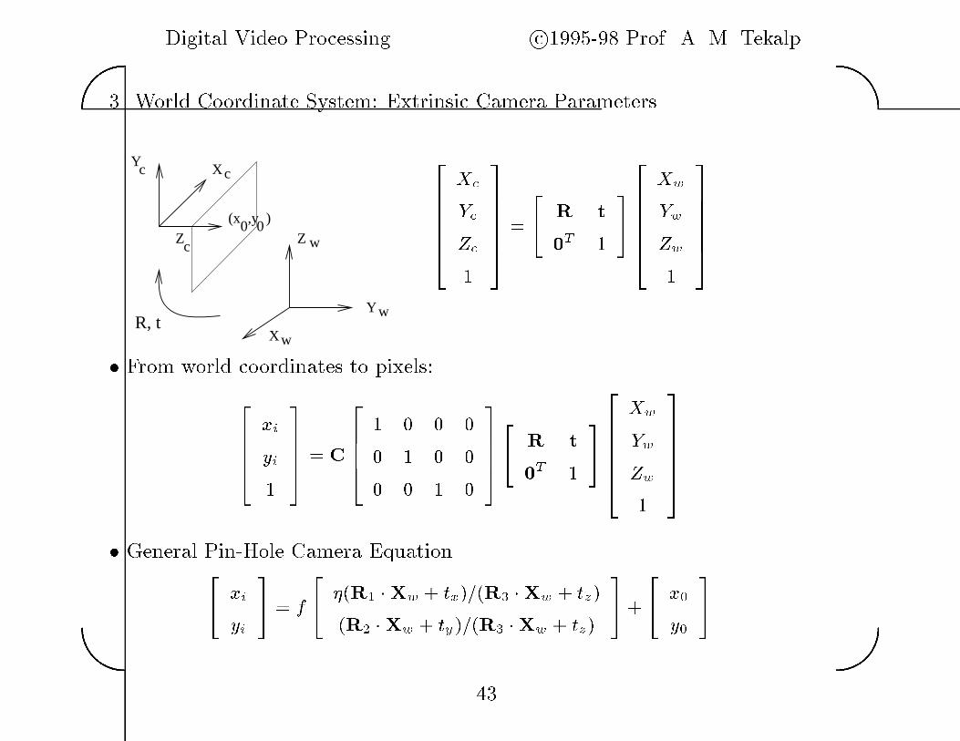
�� World Coordinate System� Extrinsic Camera Parameters
R, tX
Y
Z
XY
Z
w
w
w
c
c
c
(x ,y )0 0
������Xc
YcZc
�
������ ��
R t
�T �
��
�����Xw
YwZw
�
������
� From world coordinates to pixels�
����xi
yi�
���� � C
�����
�
� �
����
R t
�T �
��
�����Xw
YwZw
�
������
� General Pin�Hole Camera Equation�xi
yi�
� f�
��R� �Xw � tx���R� �Xw � tz�
�R� �Xw � ty���R� �Xw � tz�
��
�x�
y��
�
Digital Video Processing c�������� Prof� A� M� Tekalp��
��
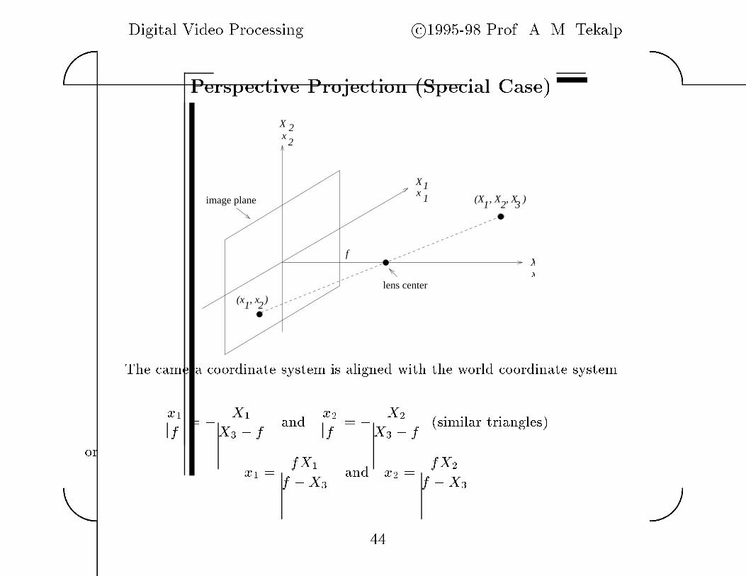
Perspective Projection �Special Case�
lens center
image plane
X 2x
2
xX
1 1
Xx
(x , x )
(X , X , X )321
1 2
f
The camera coordinate system is aligned with the world coordinate system�
x�f
� �
X�
X� � f
and
x�f
� �
X�
X� � f
�similar triangles�
or
x� �
fX�
f �X�
and x� �
fX�
f �X�

Digital Video Processing c�������� Prof� A� M� Tekalp��
��
Weak�Perspective Projection
Let Zci � R� �X �Dz then the perspective projection is given by
x � f�
��R� �X�Dx��Zc
i
�R� �X�Dy��Zc
i
��
�ox
oy�
If the average distance of the object from the camera Zcave is such that
�Zci � Zci � Zcave � R� �Xave �� Zcave
then
x �
fZcave
��RT�
R
T�
�X�
fZcave
��Dx
Dy
��
�ox
oy�
�

Digital Video Processing c�������� Prof� A� M� Tekalp��
��
A�ne Camera
An uncalibrated weak�perspective projection
����x�
x�x�
���� �
����T�� T�� T�� T��
T�� T�� T�� T��
T���
����
�����X�
X�
X�
X�
������
In Cartesian coordinates
x �MX� t
whereM is a � � � matrix with elements Mij � Tij�T�� and
t � �T���T�� T���T���
�
Digital Video Processing c�������� Prof� A� M� Tekalp��
��
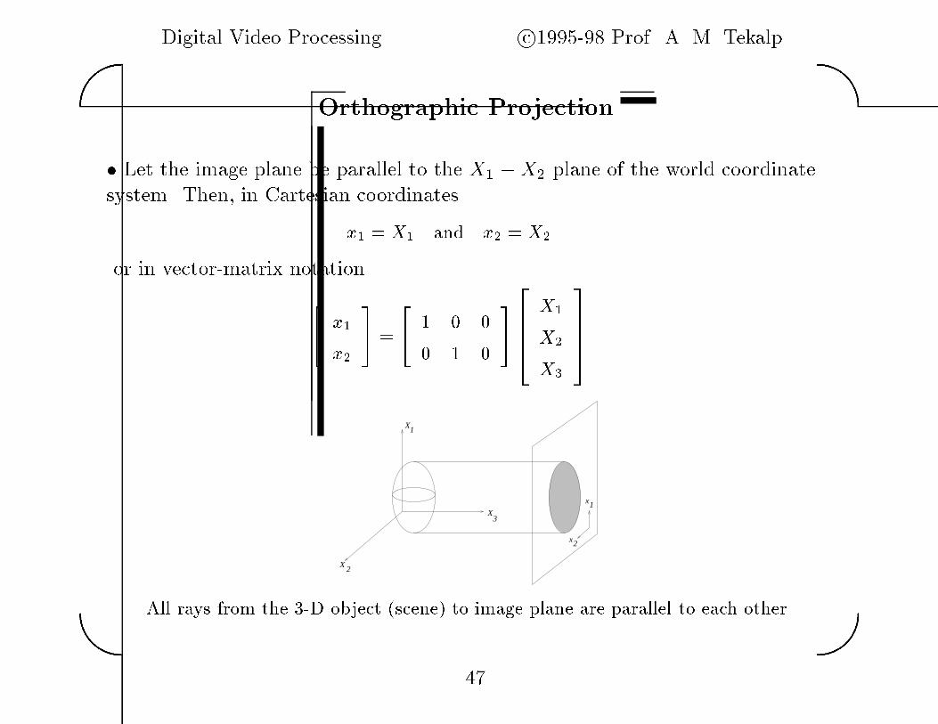
Orthographic Projection
� Let the image plane be parallel to the X� �X� plane of the world coordinate
system� Then in Cartesian coordinates
x� � X� and x� � X�
or in vector�matrix notation
�x�
x��
��
�
� �����X�
X�
X�
����
X 2
X1
X3
x2
x1
All rays from the ��D object �scene� to image plane are parallel to each other�
�
Digital Video Processing c�������� Prof� A� M� Tekalp��
��
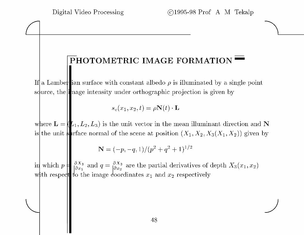
PHOTOMETRIC IMAGE FORMATION
If a Lambertian surface with constant albedo � is illuminated by a single point
source the image intensity under orthographic projection is given by
sc�x�� x�� t � �N�t � L
where L � �L�� L�� L� is the unit vector in the mean illuminant direction and N
is the unit surface normal of the scene at position �X�� X�� X��X�� X� given by
N � ��p��q� � ��p� � q� � � ���
in which p � �X
�x�
and q � �X
�x
are the partial derivatives of depth X��x�� x�
with respect to the image coordinates x� and x� respectively�
�

Digital Video Processing c�������� Prof� A� M� Tekalp��
��
L
surface normal
illumination
1s ( x , x , t)c
N (t)
2image intensity
Photometric model�
Note that the illuminant direction can also be expressed in terms of tilt and slant
angles as
L � �L�� L�� L�
� �cos � sin� sin � sin� cos
where � the tilt angle of the illuminant is the angle between L and the X� �X�
plane and the slant angle is the angle between L and the positive X� axis�
�

Digital Video Processing c�������� Prof� A� M� Tekalp��
��
Photometric E�ect of ��D Motion
Assuming that the mean illuminant direction L remains constant we can express
the change in intensity due to photometric e�ects of the motion as
dsc�x�� x�� t
dt
� �L �dN
dt
Approximate dNdt at the point �X�� X�� X� as
dNdt�
�N�t
where
�N � N�X ��� X
��� X
�� �N�X�� X�� X�
�
��p���q�� �
�p�� � q�� � � ����
��p��q� �
�p� � q� � � ����
and
p� �
�X ��
�x��
��X ��
�x��x�
�x��
���� � p
� � ��p
q� �
�X ��
�x��
���� � q
����q
��

Digital Video Processing c�������� Prof� A� M� Tekalp��
��
LECTURE �
SPATIO�TEMPORAL SAMPLING
�� Spatio�Temporal Sampling
� ��D Sampling Structures for Analog Video
� ��D Sampling Structures for Digital Video
� Analog�to�Digital Conversion
�� Spectral Characterization of Sampled Video
� ��D Sampling on a Rectangular Grid
� ��D��D Sampling on a Lattice
�� Reconstruction of Continuous Video from Samples
� Digital�to�Analog Conversion
c�������� This material is the property of A� M� Tekalp� It is intended for use only as a teaching aid when teaching
a regular semester or quarter based course at an academic institution using the textbook �Digital Video Processing�
�ISBN ���������� by A� M� Tekalp� Any other use of this material is strictly prohibited�
��

Digital Video Processing c�������� Prof� A� M� Tekalp��
��
Spatio�Temporal Sampling
RGBto
YUV
NTSC
encoder
NTSC
decoder toRGB
YUVGB
R Y
VU
signalcomposite
YUV
RGB
source display
� Consider the image plane intensity distribution scx�� x�� t� as a function of
three continuous variables� Then�
� for analog storage and transmission it is sampled in two dimensions
usually x� and t� by means of the scanning process� and
� for digital processing� storage and transmission in all three dimensions�
� Sampling the composite signal vs� component signals�
��
Digital Video Processing c�������� Prof� A� M� Tekalp��
��
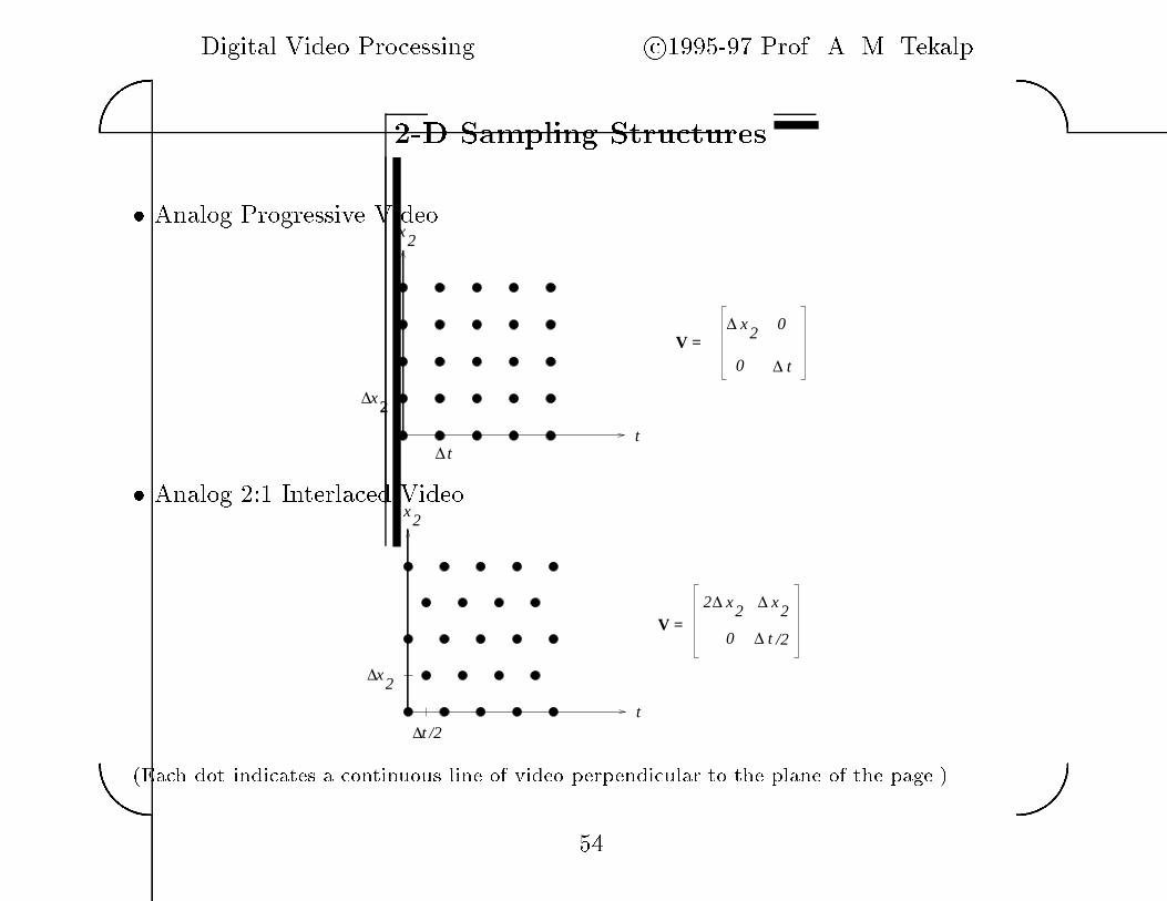
��D Sampling Structures
� Analog Progressive Video∆ 2
V =
t
x2
x
t∆
0
0∆
∆
x2
t
� Analog � � Interlaced Video
∆
V =
t
x2
2
∆
x
t /2
∆ ∆2 x2
x2
0 ∆ t /2
�Each dot indicates a continuous line of video perpendicular to the plane of the page��
��

Digital Video Processing c�������� Prof� A� M� Tekalp��
��
��D Sampling Structures
� Progressive Sampling∆
∆
∆
1 1 1 1 1
1 1 1 1 1
11111
1 1 1 1 1
11 1111
10x 0
0 0
02
x
t
V = 0
� Vertically Aligned � � Line�Interlaced Sampling∆t/2
∆
1
2
1 1 11 1
11111
1 1 1 1 1
2 2 2 2
222
2
2 2
V = 0
0
0 0
0
∆2 x∆x
x1
2 2
�Each dot indicates a pixel location� the numbers indicate the time of sampling��
��
Digital Video Processing c�������� Prof� A� M� Tekalp��
��
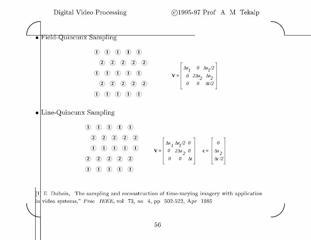
� Field�Quincunx Sampling
∆
∆ ∆
1 1 1 11 1
11111
1 1 1 1 1
22222
22222
∆
V =
0
0
0
0
/2
xx2
x x1/2
t∆
1
2 2
� Line�Quincunx Sampling
1 1 1 11 1
1 1 1 1 1
22222
11111
2 2 2 2 2
∆
∆
∆
∆
c =
∆
∆V =
0
0
0
0
0 0
x2/2t
/21
x
2 x2
t
1x
��� E� Dubois� �The sampling and reconstruction of timevarying imagery with application
in video systems� Proc� IEEE� vol� ��� no� � pp� ������� Apr� �����
��
Digital Video Processing c�������� Prof� A� M� Tekalp��
��
Analog�to�Digital Conversion
� Minimum sampling frequency is ��� � � � ��� MHz Nyquist rate�
� Sampling rate should be an integral multiple of the line rate� so that samples
in successive lines are aligned�
� For sampling the composite signal� the sampling frequency must be an
integral multiple of the subcarrier frequency� This simpli�es decoding
composite to RGB� of the sampled signal�
� For sampling component signals� there should be a single rate for ����� and
����� systems� i�e�� the sampling rate should be an integral multiple of both
����� � ��� � ������ and �� � ��� ��������
��

Digital Video Processing c�������� Prof� A� M� Tekalp��
��
Sampling the Composite Signal
NTSC NTSC PAL
� fsc SMPTE � M fsc
Bandwidth �MHz� �� �� ���
Subcarrier�sampling frequency �MHz� ��������� ������ ��� � �������
Total�active samples�line ������� ������� ��� ����
Bitrate �Mbps� ���� �� �� � ���
Sampling Component Signals
�������� ������
SMPTE ���M
Luminance Sampling frequency �MHz� ���� ����
Total�active samples�line ������� �� ����
Bitrate �Mbps� ��� ���
Chrominance Sampling frequency �MHz� ���� ����
���� Total�active samples�line ������ ������
Bitrate �Mbps� � �
��

Digital Video Processing c�������� Prof� A� M� Tekalp��
��
Chrominance Formats for Digital Video
4:4:4 4:2:2 4:2:0
Y
VV
Y Y
U UU
V��
Digital Video Processing c�������� Prof� A� M� Tekalp��
��
��D Sampling on a Rectangular Grid
With rectangular sampling� we sample at the locations
x� � n����
x� � n���
where �� and �� are the sampling distances in the x and y directions�
respectively�
The sampled signal can be expressed as
sn�� n�� � scn���� n����
��
Digital Video Processing c�������� Prof� A� M� Tekalp��
��
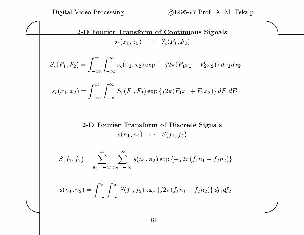
��D Fourier Transform of Continuous Signals
scx�� x�� � ScF�� F��
ScF�� F�� �Z �
��
Z ���
scx�� x�� exp f�j��F�x� � F�x��gdx�dx�
scx�� x�� �Z �
��
Z ���
ScF�� F�� exp fj��F�x� � F�x��gdF�dF�
��D Fourier Transform of Discrete Signals
sn�� n�� � Sf�� f��
Sf�� f�� �
�Xn����
�Xn����
sn�� n�� exp f�j��f�n� � f�n��g
sn�� n�� �Z �
�� ��
Z ��
� ��
Sf�� f�� exp fj��f�n� � f�n��g df�df�
��

Digital Video Processing c�������� Prof� A� M� Tekalp��
��
Spectrum of the Sampled Signal
� Evaluate the inverse Fourier transform expression at the sampling locations
sn�� n�� �Z �
��
Z ���
ScF�� F�� exp fj��F�n��� � F�n����g dF�dF�
� De�ne f� � F��� and f� � F����
sn�� n�� �Z �
��
Z ���
Scf�
���f�
��� exp fj��f�n� � f�n��g
�����df�df�
� Next� break the integration over the f�� f�� plane into a sum of integrals each
over a square denoted by SQk�� k��
s�n�� n�� �X
k�
Xk�
Z ZSQ�k��k��
�����Sc�f�
���f�
��� exp fj���f�n� � f�n��g df�df�
where SQk�� k�� is de�ned as
��
�� k� � f� ��
�� k� and ��
�� k� � f� ��
�� k�
��

Digital Video Processing c�������� Prof� A� M� Tekalp��
��
� A change of variablesf �� � f� � k�� and f �� � f� � k�
shifts all the squares SQk�� k�� down to � �� ��
� �� � �� ��
� ��
sn�� n�� �
Z ��
�
��
Z ��
�
��f
�����
Xk�
Xk�
Scf� � k�
��
�f� � k�
��
�g
exp fj��f�n� � f�n��g exp f�j��k�n� � k�n��g df�df�
� But� exp f�j��k�n� � k�n��g � � for k�� k�� n�� n� integers� Thus� the
frequencies f�� k�� f�� k�� map onto f�� f��� Compare the last expression with
sn�� n�� �Z �
�� ��
Z ��
� ��
Sf�� f�� exp fj��f�n� � f�n��g df�df�
� to conclude that
Sf�� f�� �
�����
Xk�
Xk�
Scf� � k�
��
�f� � k�
��
�
for � �� � f�� f� ��
� �
��
Digital Video Processing c�������� Prof� A� M� Tekalp��
��
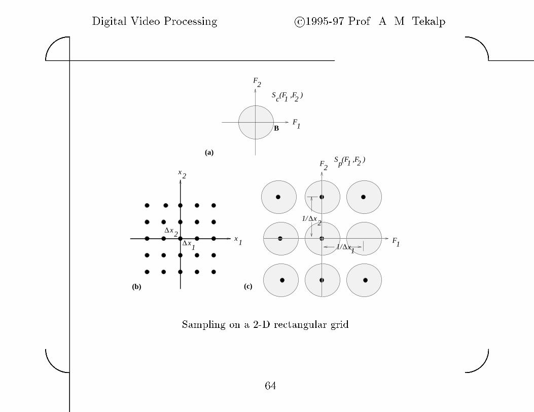
∆
B
∆
∆
∆
x1
x2
x2
x1
F1
F2
S (F ,F )1 2c
p 1S (F ,F )2
F1
F2
1/ x2
1/1x
(a)
(c)(b)
Sampling on a ��D rectangular grid
��
Digital Video Processing c�������� Prof� A� M� Tekalp��
��
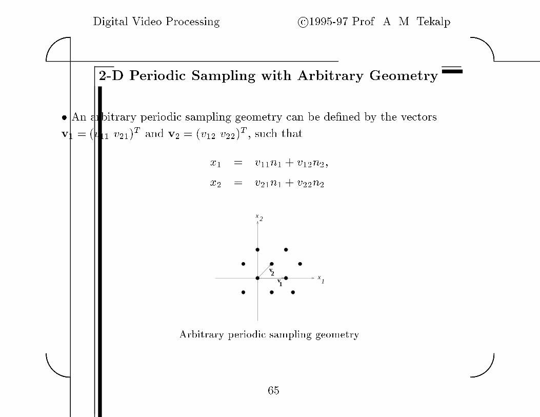
��D Periodic Sampling with Arbitrary Geometry
� An arbitrary periodic sampling geometry can be de�ned by the vectors
v� � v�� v���T and v� � v�� v���T � such that
x� � v��n� � v��n��
x� � v��n� � v��n�
v
v
1
2
x 2
x1
Arbitrary periodic sampling geometry
��
Digital Video Processing c�������� Prof� A� M� Tekalp��
��
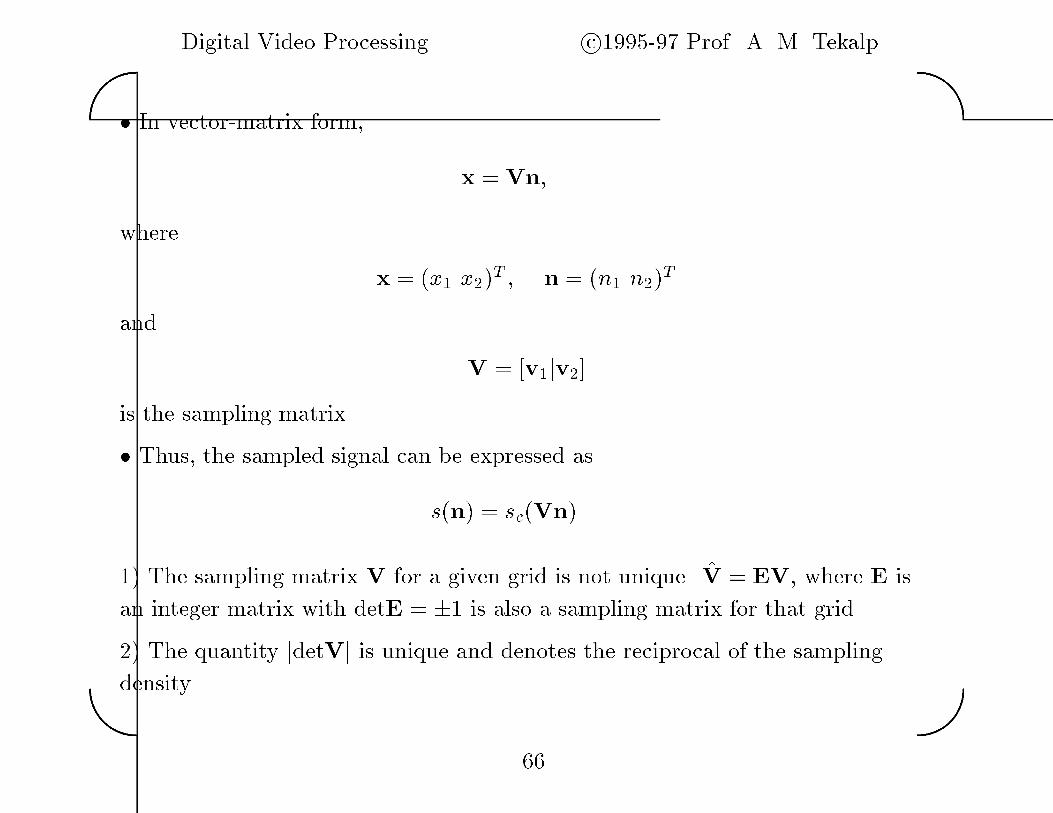
� In vector�matrix form�
x � Vn�
where
x � x� x��T � n � n� n��T
and
V � �v�jv��
is the sampling matrix�
� Thus� the sampled signal can be expressed as
sn� � scVn�
�� The sampling matrix V for a given grid is not unique� �V � EV� where E is
an integer matrix with detE � �� is also a sampling matrix for that grid�
�� The quantity jdetVj is unique and denotes the reciprocal of the sampling
density�
��
Digital Video Processing c�������� Prof� A� M� Tekalp��
��
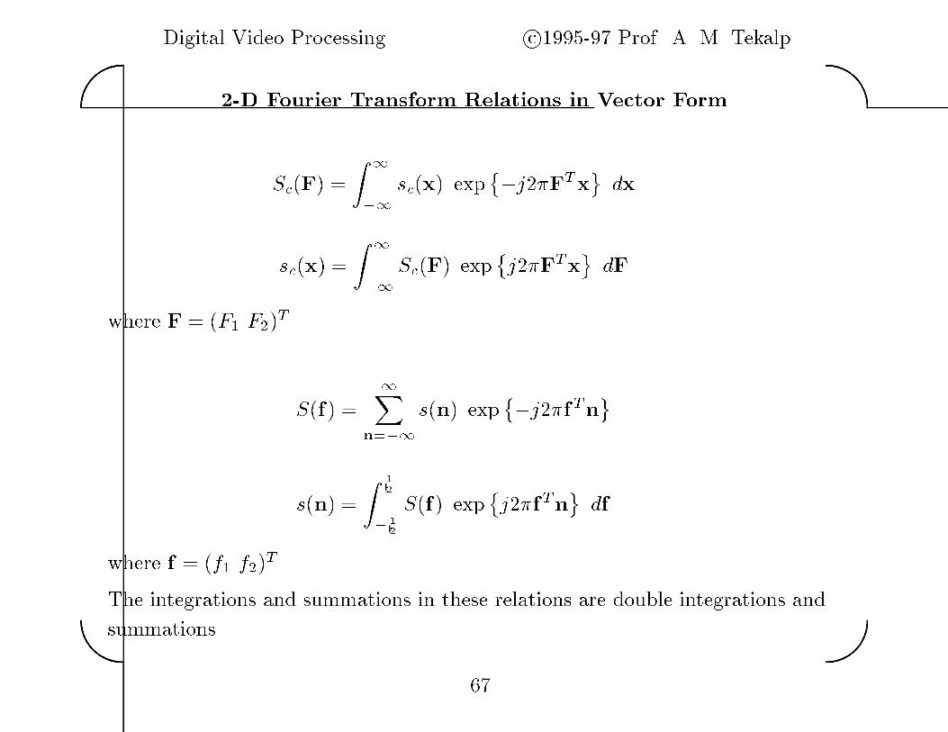
��D Fourier Transform Relations in Vector Form
ScF� �Z �
��
scx� exp�
�j��FTx�
dx
scx� �Z �
��
ScF� exp�
j��FTx�
dF
where F � F� F��T �
Sf� �
�Xn���
sn� exp�
�j��fTn�
sn� �Z �
�� ��
Sf� exp�
j��fTn�
df
where f � f� f��T �
The integrations and summations in these relations are double integrations and
summations�
��

Digital Video Processing c�������� Prof� A� M� Tekalp��
��
Spectrum of the Sampled Signal
� Similar to the case of rectangular sampling� express
sn� � scVn� �Z �
��
ScF� exp�
j��FTVn�
dF
� Making the change of variables f � VTF�
sn� �Z �
��
�jdetVjScVT�� f� exp�
j��fTn�
df
where df � jdetVjdF using the Jacobian�
� Expressing the integration over the f plane as a sum of integrations over the
squares � �� ��
� �� � �� ��
� �� we have
sn� �Z �
�� ��
Xk
�jdetVjScVT��f � k�� exp�
j��fTn�
exp�
�j��kTn�
df
where exp�
�j��kTn�
� � for k an integer valued vector�
��

Digital Video Processing c�������� Prof� A� M� Tekalp��
��
� Comparing this expression with
sn� �Z �
�� ��
Sf� exp�
j��fTn�
df
we conclude that
Sf� �
�jdetVj
Xk
ScVT��f � k��
� or equivalently
SpF� �
�jdetVj
Xk
ScF�Uk�
where the periodicity matrix U satis�es
UTV � I
and I is the identity matrix� The periodicity matrix can be expressed as
U � �u�ju��� where u� and u� are the periodicity vectors�
� Note that the above formulation is also valid for rectangular sampling with
the matrices V and U diagonal�
��
Digital Video Processing c�������� Prof� A� M� Tekalp��
��
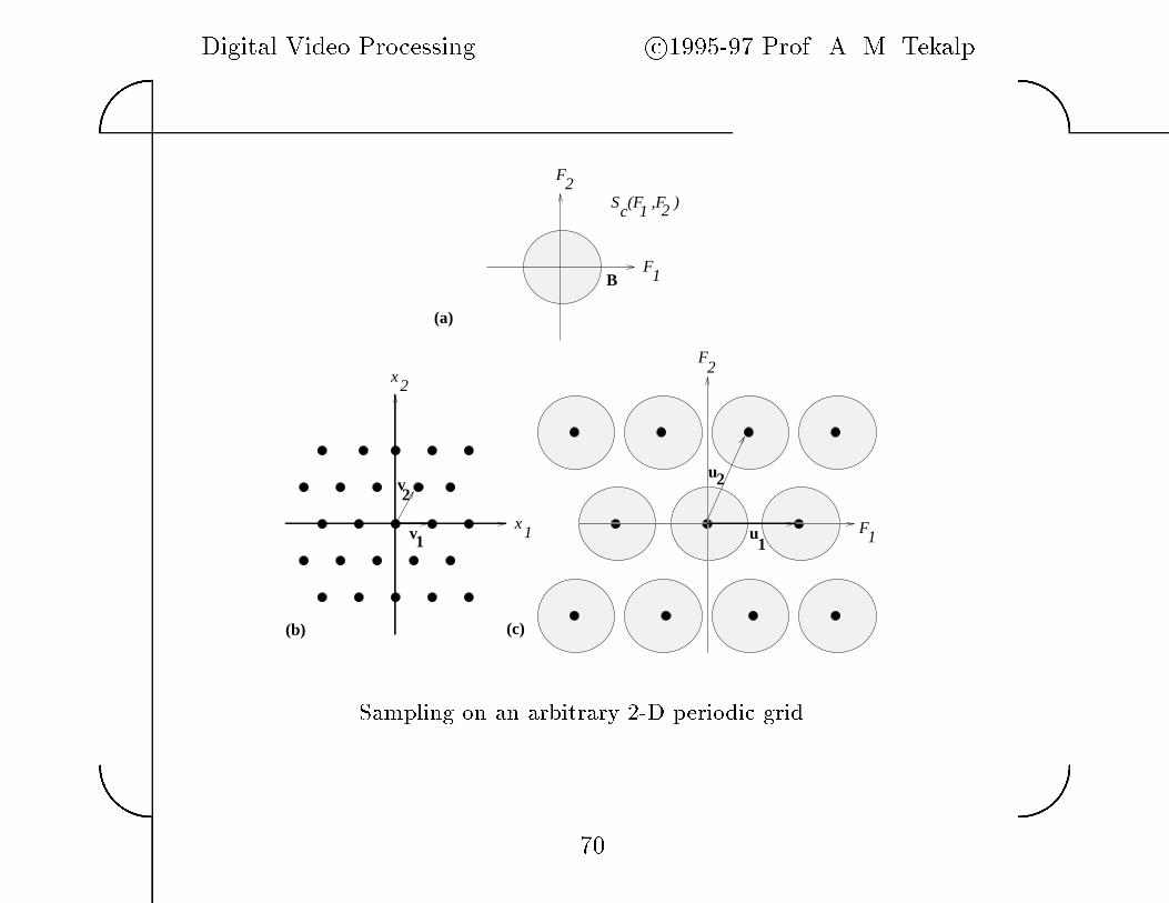
v
v
u
u
11
22
B
(a)
(b) (c)
2x
x1
F2
1 F
S (F ,F )c 1 2
F2
F1
Sampling on an arbitrary ��D periodic grid
��

Digital Video Processing c�������� Prof� A� M� Tekalp��
��
Sampling on ��D Lattices
� Let v��v��v� be linearly independent vectors in the ��D Euclidean space R��
A lattice � in R� is the set of all linear combinations of v��v��v� with integer
coe�cients
� � fn�v� � n�v� � kv� j n�� n�� k � Zg
� In vector�matrix notation� let V be the sampling matrix
V � �v�jv�jv���
then
� � fV�n� n� k�T j n�� n�� k� � Z�g
� A spatio�temporal signal scx� t� sampled on a lattice � can be expressed as
sn� k� � scV�n� n� k�T �� n�� n�� k� � Z�
Observe that d�� � jdetV�j denotes the reciprocal of the sampling density�
and V is not unique�
��
Digital Video Processing c�������� Prof� A� M� Tekalp��
��
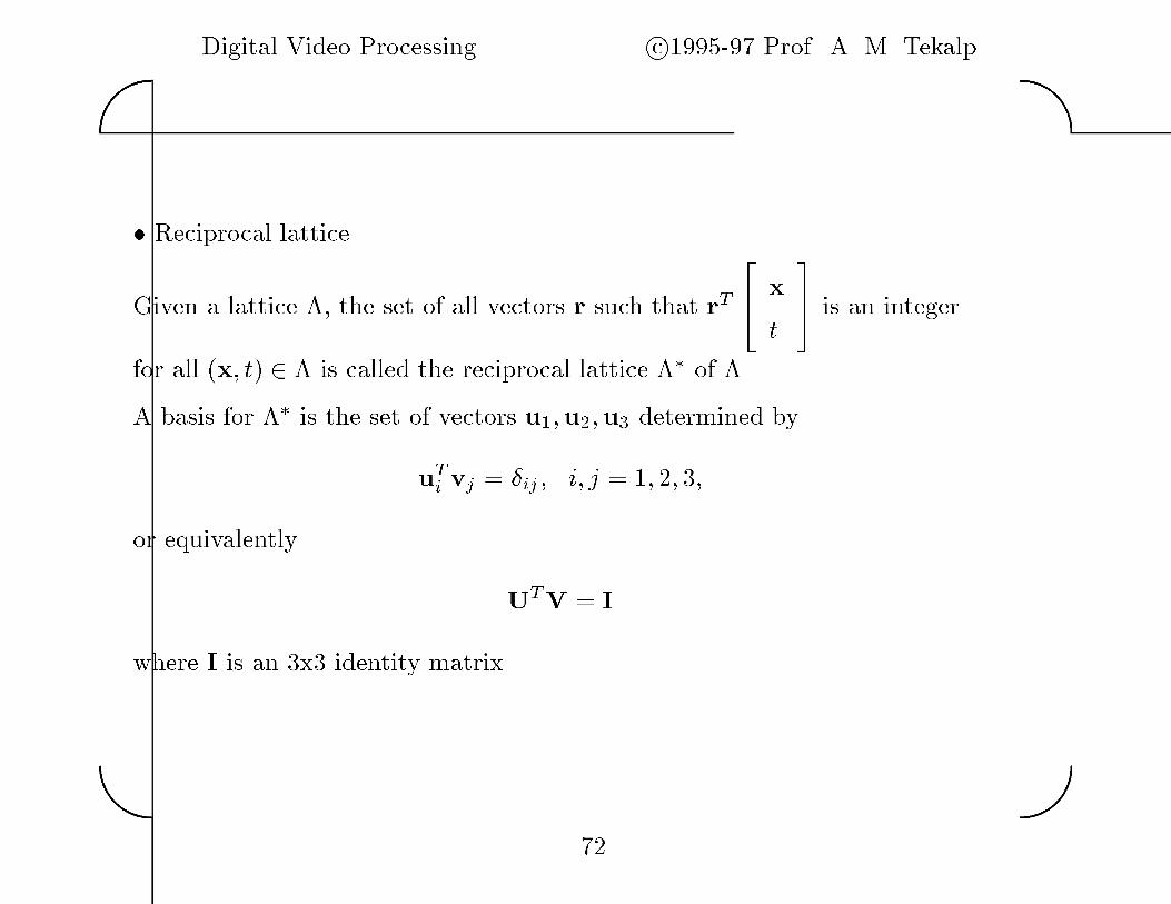
� Reciprocal lattice
Given a lattice �� the set of all vectors r such that rT�
� xt
�� is an integer
for all x� t� � � is called the reciprocal lattice �� of ��
A basis for �� is the set of vectors u��u��u� determined by
uTi vj � �ij� i� j � �� �� ��
or equivalently
UTV � I
where I is an �x� identity matrix�
��

Digital Video Processing c�������� Prof� A� M� Tekalp��
��
� Unit Cell Voronoi cell�
The set of points that are closer to the origin than to any other sample point�
2x
1x
��

Digital Video Processing c�������� Prof� A� M� Tekalp��
��
Fourier Transform on a Lattice
Let sn� k� � scV�n� n� k�T �� n�� n�� k� � Z�� then
Sf� �
X�n�k��Z
sn� k� exp��
�j��fT�
� nk
��
�� � f � R�
and
sn� k� �Z �
�� ��
Sf� exp��
j��fT�
� nk
��
�� df n� k� � Z�
where f � VTF is the normalized frequency�
� The Fourier transform of a signal sampled on a lattice � is periodic with the
replications centered at the sites of the reciprocal lattice ��� Note that
f � � �� ��
� �� � �� ��
� �� � �� ��
� � implies that F � �F� F� Ft�T � P � where P
denotes the unit cell of the reciprocal lattice ���
��

Digital Video Processing c�������� Prof� A� M� Tekalp��
��
Spectrum of Signals Sampled on a Lattice
� Suppose that scx� � L�RM �
ScF� �Z
Rscx� t� exp
���j��FT
�� x
t�
��
�dx dt� F � R�
with the inverse transform
scx� t� �Z
RScF� exp
��j��FT
�� x
t�
��
�dF� x� t� � R�
� The Fourier transform of the sampled signal is equal to an in�nite sum of
copies of the analog spectrum shifted according to the reciprocal lattice ��
SpF� �
�d��
Xk�Z
ScF�Uk�
where
UTV � I��

Digital Video Processing c�������� Prof� A� M� Tekalp��
��
Example� Progressive and the � � line interlaced sampling lattices�
(a) (b)
∆
∆
t
t /2
The periodicity matrices indicating the locations of the replications
Upro � V��T
pro ��
��
�x�
��x�
��t
���� and Uint � V��T
int ��
��
�x�
���x�
� ��t
��t
����
��
Digital Video Processing c�������� Prof� A� M� Tekalp��
��
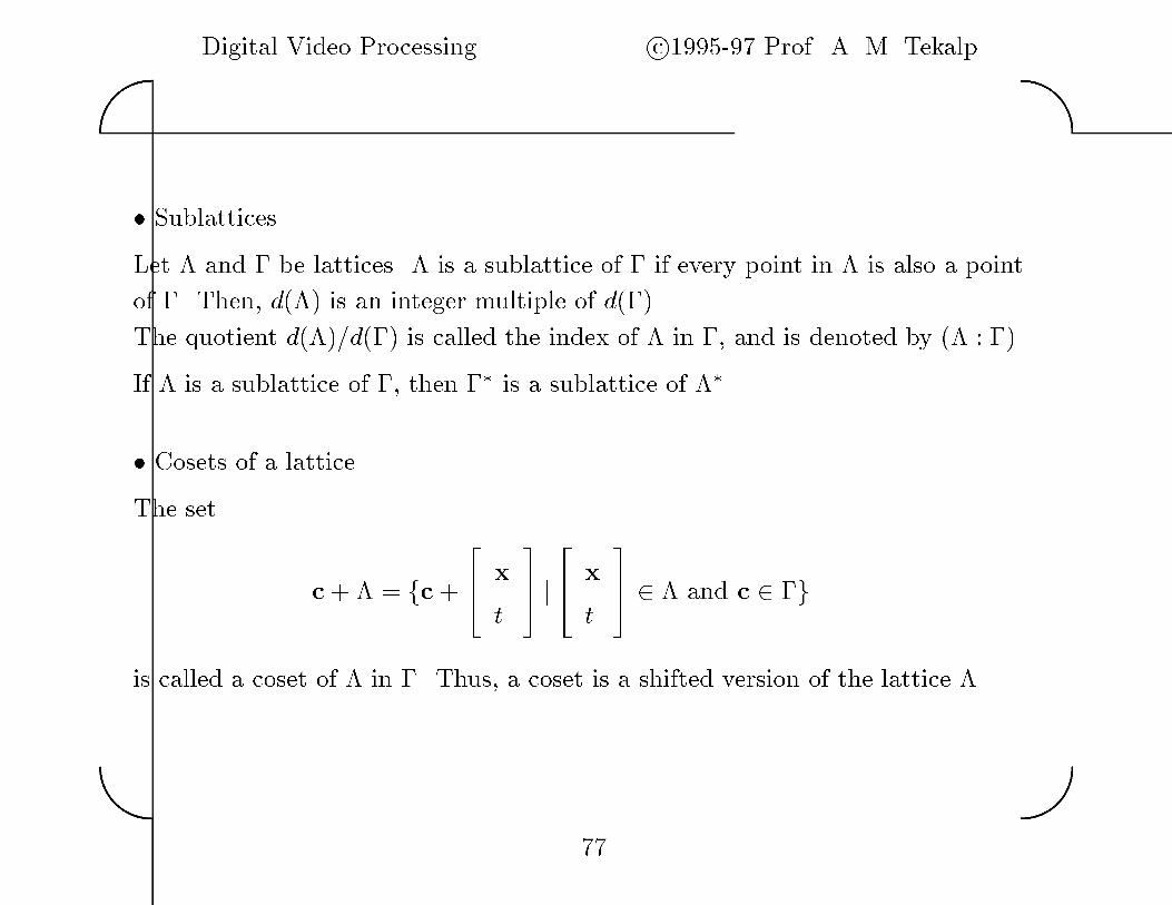
� Sublattices
Let � and � be lattices� � is a sublattice of � if every point in � is also a point
of �� Then� d�� is an integer multiple of d���
The quotient d���d�� is called the index of � in �� and is denoted by � ���
If � is a sublattice of �� then �� is a sublattice of ���
� Cosets of a lattice
The set
c� � � fc��
� xt
�� j
�� x
t�
� � � and c � �g
is called a coset of � in �� Thus� a coset is a shifted version of the lattice ��
��
Digital Video Processing c�������� Prof� A� M� Tekalp��
��
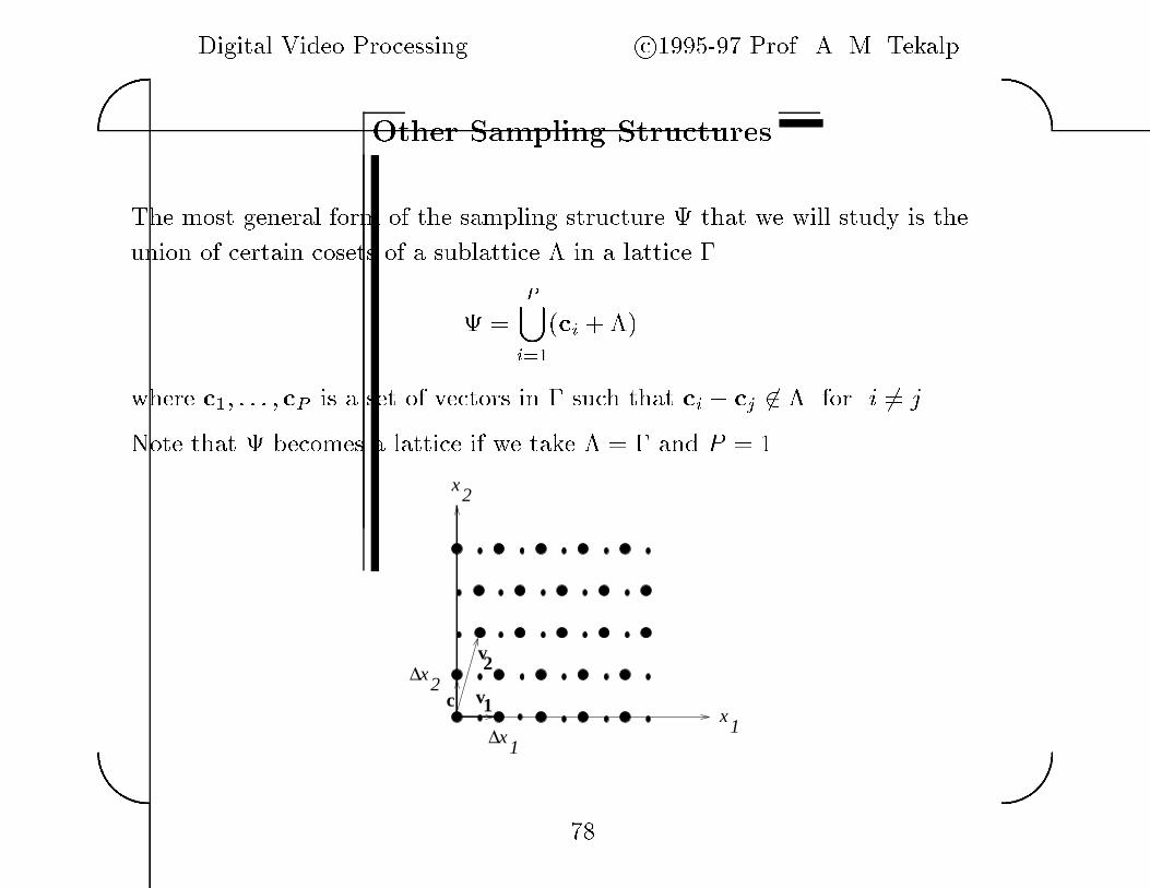
Other Sampling Structures
The most general form of the sampling structure � that we will study is the
union of certain cosets of a sublattice � in a lattice �
� �
P�i��
ci � ��
where c�� � � � � cP is a set of vectors in � such that ci � cj � � for i � j�
Note that � becomes a lattice if we take � � � and P � ��
∆
∆
c
v2
1v
x2
x1
1x
2x
��

Digital Video Processing c�������� Prof� A� M� Tekalp��
��
Spectrum of Signals Sampled on a Structure �
SpF� �
�d��
Xk
gk�ScF�Uk�
The function
gk� �
PXi��
exp�
j��kTUT ci�
is constant over cosets of �� in ��� and may be zero for some of these cosets�
so the corresponding shifted versions of the analog spectrum are not present�
F
F1
2
Reciprocal lattice ��
��
Digital Video Processing c�������� Prof� A� M� Tekalp��
��
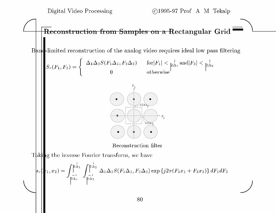
Reconstruction from Samples on a Rectangular Grid
Band�limited reconstruction of the analog video requires ideal low pass �ltering
Sr�F�� F�� ��
����S�F���� F���� forjF�j �
����andjF�j �
����
otherwise
1/2∆
1/2∆
x2
x1
F2
F1
Reconstruction �lter
Taking the inverse Fourier transform� we have
sr�x�� x�� �Z �
� �
��
� �
Z �� �
��
� �
����S�F���� F���� exp fj���F�x� � F�x��g dF�dF�
��

Digital Video Processing c�������� Prof� A� M� Tekalp��
��
� Substituting the de�nition of SF���� F����
sr�x�� x�� �
Z �� �
��
� �
Z �� �
��
� �
����fX
n�
Xn�
s�n�� n��
exp f�j���F���n� � F���n��gg exp fj���F�x� � F�x��g dF�dF�
� Rearranging the terms� we have
sr�x�� x�� � ����X
n�
Xn�
s�n�� n��Z �
� �
��
� �
Z �� �
��
� �
exp f�j���F���n� � F���n��g
exp fj���F�x� � F�x��g dF�dF�
� Note that the integral evaluates to
hx�� x�� �sinh
���x� � n����i
���x� � n����
sinh
���x� � n����i
���x� � n����
which is the ideal interpolation function for rectangular sampling�
��

Digital Video Processing c�������� Prof� A� M� Tekalp��
��
Reconstruction from Samples on a Lattice
� Exact reconstruction of a continuous signal from its samples on a lattice � is
possible via ideal low�pass �ltering over a unit cell P of �� provided that the
original continuous image spectrum was con�ned to this unit cell�
� The ideal low pass �ltering can be expressed as
SrF� ���
jdetVjSVTF� for F � P
� otherwise�
� In the space domain� we have
srx� t� �
X�n�k��Z
sn� k�h�
� xt
���V
�� n
k�
��
where
hx� � jdetVjZ
P
exp��
j��FT�
� xt
��
�� dF
Here hx� is the ideal interpolation function for the particular lattice geometry�
��
Digital Video Processing c�������� Prof� A� M� Tekalp��
��
LECTURE �
SAMPLING STRUCTURE CONVERSION
�� Video Standards Conversion
�� Interpolation and Decimation of ��D Signals
�� Theory of Sampling Structure Conversion
c�������� This material is the property of A� M� Tekalp� It is intended for use only as a teaching aid when teaching
a regular semester or quarter based course at an academic institution using the textbook �Digital Video Processing�
�ISBN ���������� by A� M� Tekalp� Any other use of this material is strictly prohibited�
�

Digital Video Processing c�������� Prof� A� M� Tekalp��
��
Sampling Structure Conversion
Sampling Structure
ConversionεΛ3
s (x , x , t) p
(x , x , t)
y (x , x , t) p
(x , x , t)1
εΛ321 2
2
2
1 21
1
This is a spatio�temporal interpolationdecimation problem�
Applications
� Frame�Rate Conversion
� Deinterlacing �interlaced � progressive�
� Interlacing
� NTSC�to�PAL transcoding or vice versa
� Data Compression �U V subsampling�
�

Digital Video Processing c�������� Prof� A� M� Tekalp��
��
Fundamentals of Decimation�Interpolation
s (n) u(n) w(n) y (n) Low pass DownsampleUpsample
1:L M:1 filterSampling rate change by a rational factor LM
�
� Characterization in the Frequency�Domain
� Filter Design for InterpolationDecimation
��� A� V� Oppenheim and R� W� Schafer� Discrete�Time Signal Processing� Prentice Hall�
NJ� �����
�
Digital Video Processing c�������� Prof� A� M� Tekalp��
��
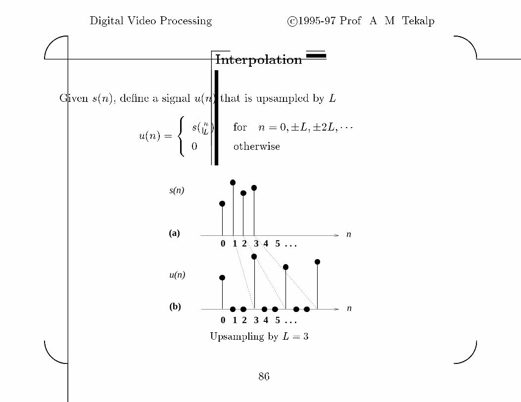
Interpolation
Given s�n� de�ne a signal u�n� that is upsampled by L
u�n� ���
�s� nL� for n � ���L���L� � � �
� otherwise�
0 1 2 3 4 5 . . .
0 1 2 3 4 5 . . .
s(n)
u(n)
n
n
(a)
(b)
Upsampling by L � ��
�

Digital Video Processing c�������� Prof� A� M� Tekalp��
��
Spectrum of the Upsampled Signal
U�f� �
�Xn���
u�n�e�j��fn �
�Xn���
s�n�e�j��fLn � S�fL�
0 -1/2
0 1/2-1/2
1/6-1/6 1/2
S(f)
U(f)
f
f
(a)
(b)
Upsampling by L � ��
�

Digital Video Processing c�������� Prof� A� M� Tekalp��
��
Ideal Interpolation Filter
Ideal interpolation �lter is an ideal lowpass �lter�
0
0 1/2L 1-1 1/2-1/2
. . .
. . .. . .
. . .
-1 1
H(f)
f
f
(b)
Y(f)
(a)
U(f)
Interpolation by L � ��
The impulse response of the ideal interpolation �lter is a sinc function� Because
of its zero�crossings it will not alter the existing signal samples while assigning
values for the zero samples in the upsampled signal�

Digital Video Processing c�������� Prof� A� M� Tekalp��
��
Practical Interpolation Filters
� Zero�order hold �sample repeat�
1
0 1 2
h(n)
n
n
u(k) k
h(n-k)
The impulse response for L � ��
� Linear interpolation
12/3
1/3
2/31/3
n
k
h(n-k)
u(k)
h(n)
n
The impulse response for L � ��
�
Digital Video Processing c�������� Prof� A� M� Tekalp��
��
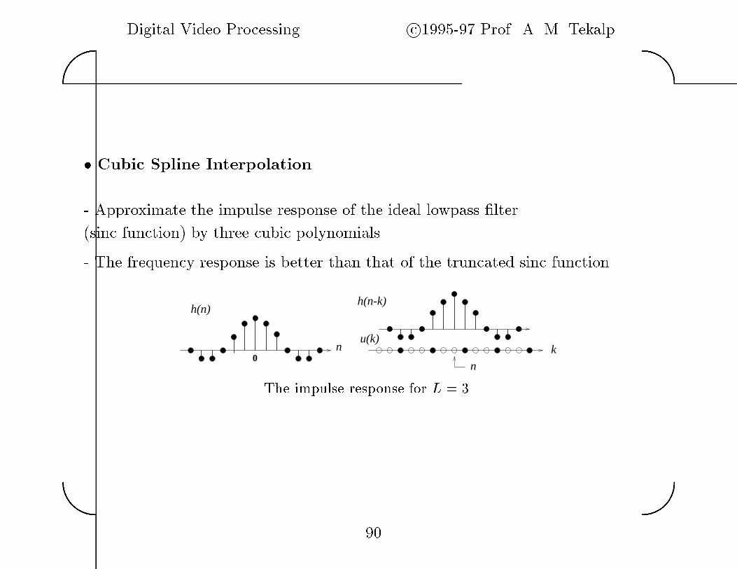
� Cubic Spline Interpolation
� Approximate the impulse response of the ideal lowpass �lter
�sinc function� by three cubic polynomials�
� The frequency response is better than that of the truncated sinc function�
0n
ku(k)
h(n-k)h(n)
n
The impulse response for L � ��
��
Digital Video Processing c�������� Prof� A� M� Tekalp��
��
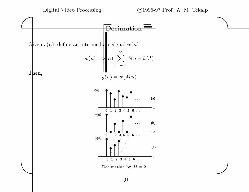
Decimation
Given s�n� de�ne an intermediate signal w�n�
w�n� � s�n�
�Xk���
��n� kM�
Then
y�n� � w�Mn�
0 1 2 3 4 5 6 . . .
. . .
0 1 2 3 4 5 6 . . .
0 1 2 3 4 5 6 . . .
. . .
. . .
s(n)
w(n)
y(n)
n
n
n
(a)
(b)
(c)
Decimation by M � �
��
Digital Video Processing c�������� Prof� A� M� Tekalp��
��
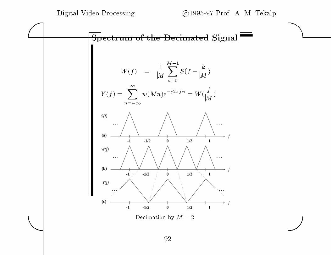
Spectrum of the Decimated Signal
W �f� �
�M
M��Xk��
S�f �
kM�
Y �f� �
�Xn���
w�Mn�e�j��fn �W �f
M�
0 1/2 1-1 -1/2
-1 -1/2
-1 -1/2
0 1/2 1
0 1/2 1
. . .
. . .
. . .
. . .
. . .
. . .
S(f)
W(f)
Y(f)
f
f
f(a)
(b)
(c)
Decimation by M � �
��

Digital Video Processing c�������� Prof� A� M� Tekalp��
��
Decimation Filters
To avoid aliasing lowpass �lter the signal before decimation�
0 1/2 1-1 -1/2
-1 -1/2
-1 -1/2
0 1/2 1
0 1/2 1
. . .
. . .
. . .
. . .
. . . . . .
Decimation filter
S(f)
W(f)
Y(f)
f
f
f
Antialias �ltering for M � ��
Box �lters are generally used instead of ideal lowpass �lters for simplicity�
��

Digital Video Processing c�������� Prof� A� M� Tekalp��
��
Rate Change by a Rational Factor
s (n) u(n) w(n) y (n) Low pass DownsampleUpsample
1:L M:1 filterRate change by a factor of L�M �
� A single lowpass �lter with cuto� frequency
fc � minf ��M � ��Lg
is su�cient�
� When L � M the requirement to preserve the values of the existing samples
must be incorporated into the �lter design���
Digital Video Processing c�������� Prof� A� M� Tekalp��
��
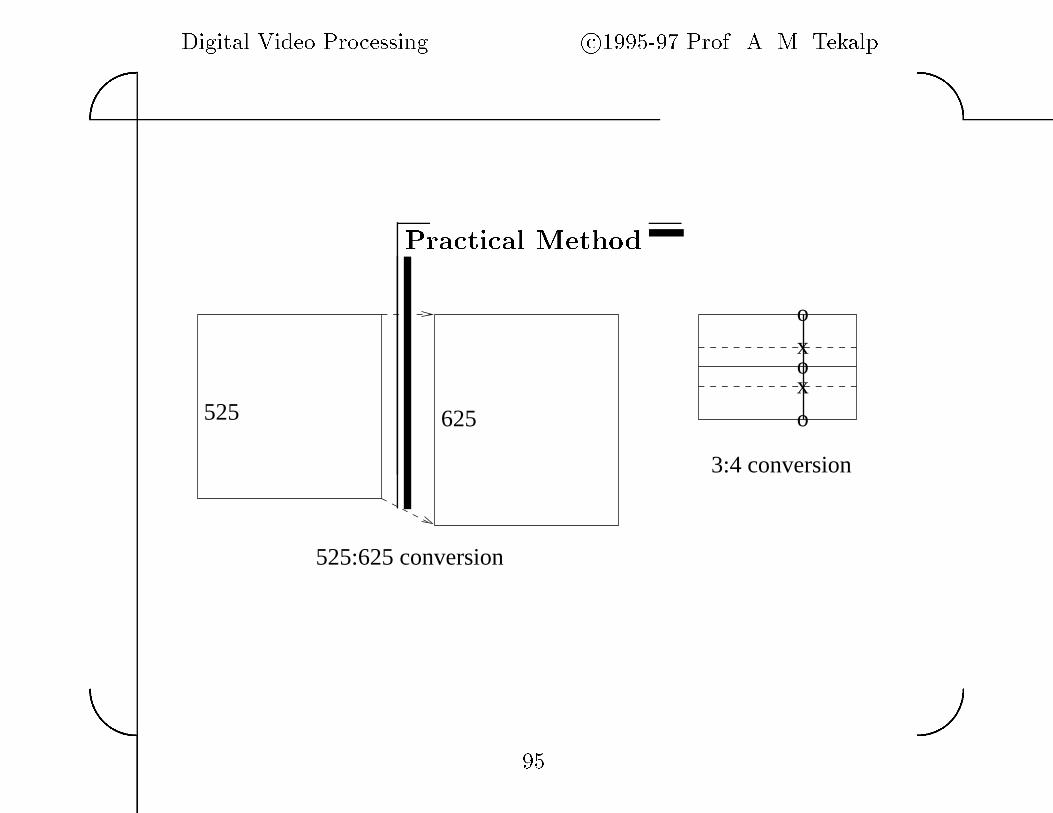
Practical Method
625525
x
xo
o
o
3:4 conversion
525:625 conversion
��
Digital Video Processing c�������� Prof� A� M� Tekalp��
��
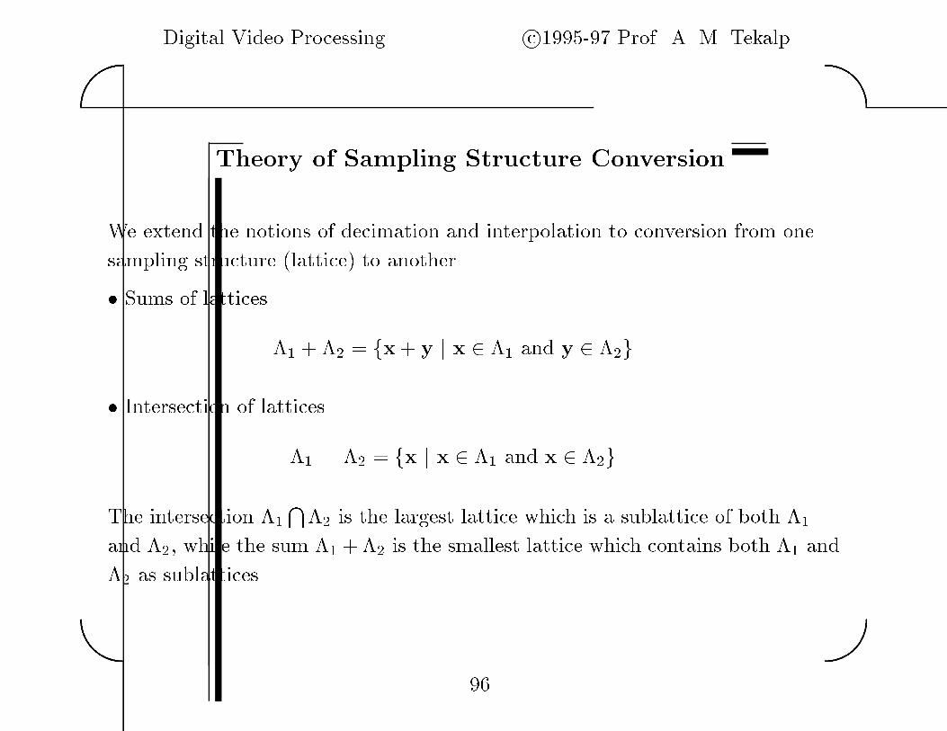
Theory of Sampling Structure Conversion
We extend the notions of decimation and interpolation to conversion from one
sampling structure �lattice� to another�
� Sums of lattices�� � �� � fx� y j x � �� and y � ��g
� Intersection of lattices
���
�� � fx j x � �� and x � ��g
The intersection ��T
�� is the largest lattice which is a sublattice of both ��
and �� while the sum �� ��� is the smallest lattice which contains both �� and
�� as sublattices�
��

Digital Video Processing c�������� Prof� A� M� Tekalp��
��
U D 3
Low pass DownconvertUpconvert filter
Λ3ε
Λ Λ+ε33
Λ Λ+ε33
Λε
s (x , x , t)p 1 2
(x , x , t)1 2 1
u (x , x , t) 1 2
wp(x , x , t)1 2
(x , x , t)21
(x , x , t)21 21 1 2
y p (x , x , t)1 2
(x , x , t)1 2 2
p
Decomposition of the system for sampling structure conversion�
De�neup�x� t� � Usp�x� t� �
���
sp�x� t� �x� t� � ��
� �x� t� �� ��� x� t� � �� ���
and
yp�x� t� � Dwp�x� t� � wp�x� t�� �x� t� � ��
Condition for the shift invariance of the �lter� if the input is shifted by q the
output should also be shifted by q� We need q � ��T
��� Thus we assume that
��T
�� is a lattice i�e� V��
� V� is a matrix of integers�
��
Digital Video Processing c�������� Prof� A� M� Tekalp��
��
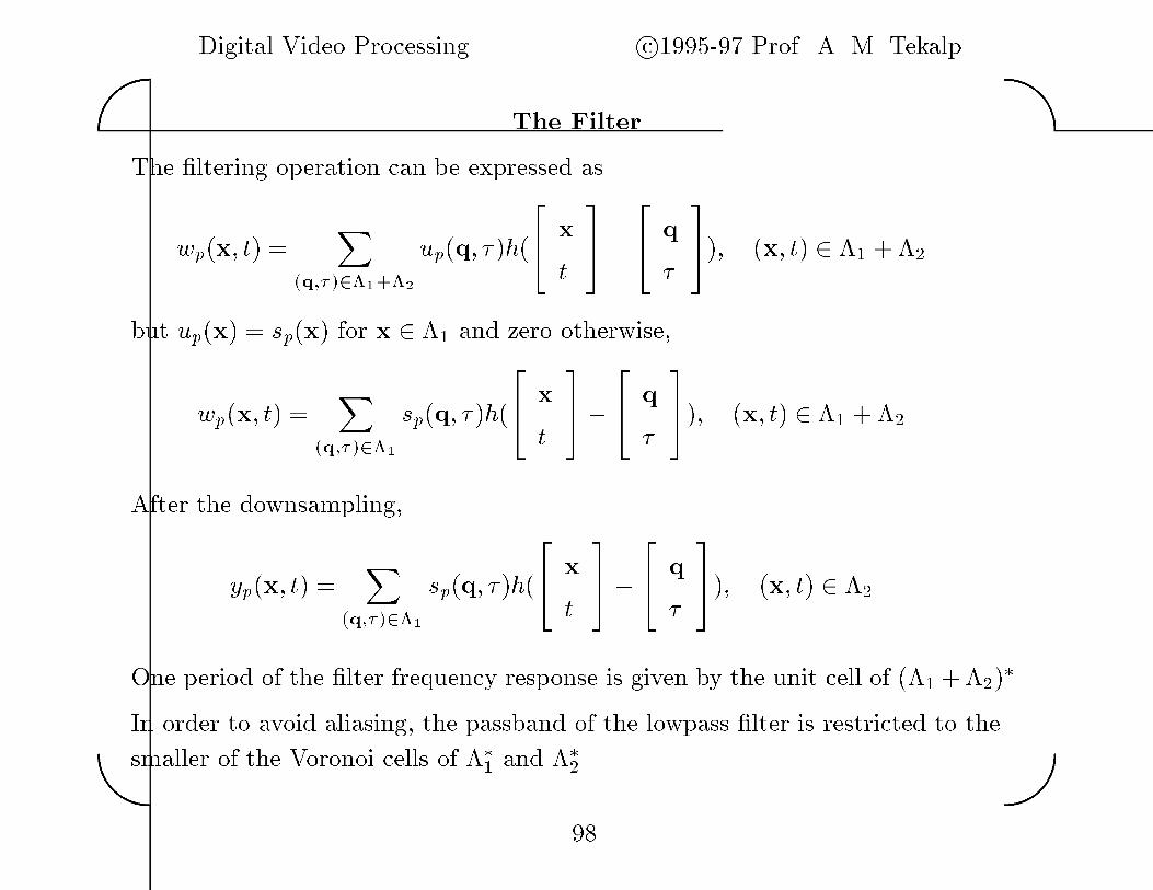
The Filter
The �ltering operation can be expressed as
wp�x� t� �
X�q���������
up�q� ��h��
� xt
���
�� q
�
���� �x� t� � �� ���
but up�x� � sp�x� for x � �� and zero otherwise
wp�x� t� �
X�q������
sp�q� ��h��
� xt
���
�� q
��
��� �x� t� � �� � ��
After the downsampling
yp�x� t� �
X�q������
sp�q� ��h��
� xt
���
�� q
��
��� �x� t� � ��
One period of the �lter frequency response is given by the unit cell of ��� ������
In order to avoid aliasing the passband of the lowpass �lter is restricted to the
smaller of the Voronoi cells of ��� and �����
Digital Video Processing c�������� Prof� A� M� Tekalp��
��
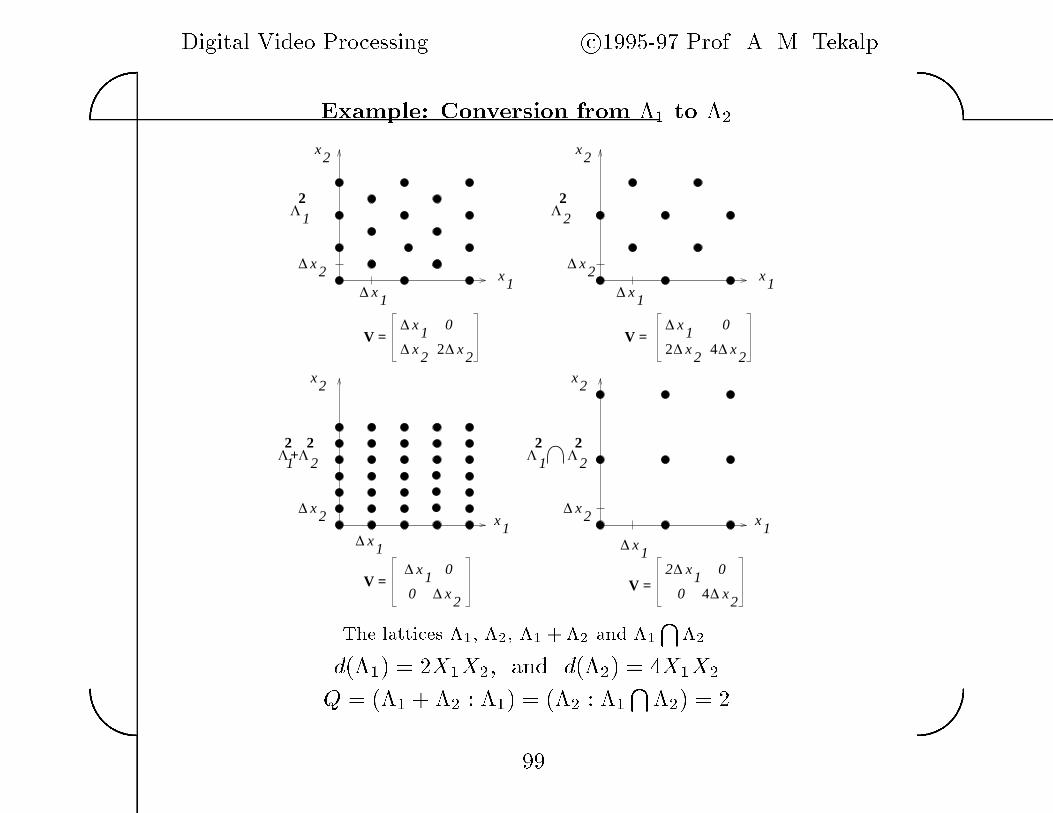
Example� Conversion from �� to ��
ΛΛ
+ΛΛ ΛΛ
∆
∆
∆
∆∆
∆
∆
∆
V = ∆
∆
∆
V = ∆
∆
V = ∆
∆
V = ∆
∆
22
2 2 2 2
x
1x
2
x2
1
x1
0 x1
x2
x2
x1
x2
2
1 x
x2
x1
0
∆ x2
x2
1 2
x2
x1
x1
x2
2 x1
0
0 x2
x2
x1
21
x2
x1
x1
0
0 x2
4
2 42The lattices �� �� � � � and �T
��
d���� � �X�X� and d���� � �X�X�
Q � ��� � �� � ��� � ��� � ��T
��� � �
��
Digital Video Processing c�������� Prof� A� M� Tekalp��
��
∆x1
Λ* Λ*
∆
∆
F2
F11/ x
1
1/ x2
1 F2
F1
2
U = 1/2-1/ ∆x1
0 x∆ 21/2
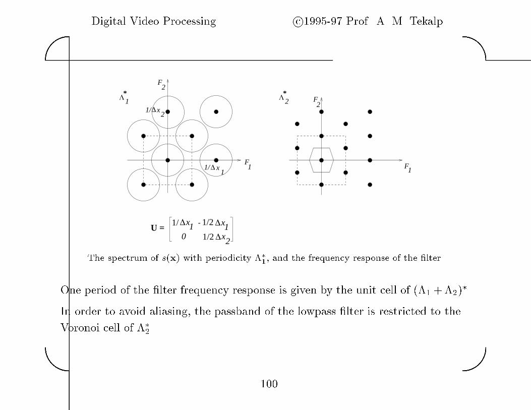
The spectrum of s�x with periodicity ��� and the frequency response of the �lter�
One period of the �lter frequency response is given by the unit cell of ��� ������
In order to avoid aliasing the passband of the lowpass �lter is restricted to the
Voronoi cell of ����
���
Digital Video Processing c�������� Prof� A� M� Tekalp��
��
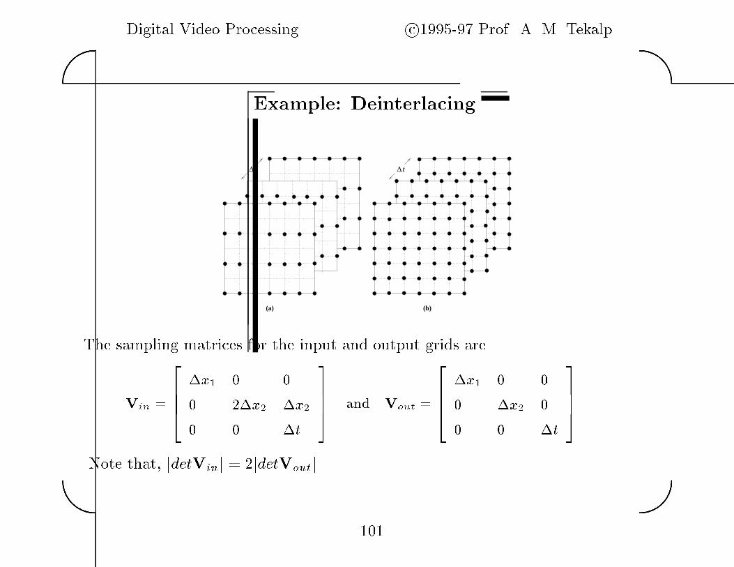
Example� Deinterlacing
(a) (b)
∆ t ∆ t
The sampling matrices for the input and output grids are
Vin ��
�x�
�x� x�
t
�� and Vout �
��x�
x�
t�
�
Note that jdetVinj � �jdetVoutj�
���

Digital Video Processing c�������� Prof� A� M� Tekalp��
��
Comments on Direct Methods
� In direct methods for sampling structure down�conversion there is a tradeo�
between allowed aliasing errors and loss of resolution �blurring� due to lowpass
�ltering prior to down�conversion�
� When lowpass �antialias� �ltering has been used prior to down�conversion the
resolution cannot be recovered by interpolation�
� Motion�compensated interpolation schemes make it possible to
recover higher resolution frames in the process of up�conversion if no antialias
�ltering has been applied prior to down�conversion�
���
Digital Video Processing c�������� Prof� A� M� Tekalp��
��
LECTURE �
OPTICAL FLOW METHODS
�� Projected Motion vs� Optical Flow
�� Occlusion and Aperture Problems
�� Optical Flow Equation
� Two�D Motion Field Models Nonparametric vs� Parametric
�� Lucas�Kanade Method
�� Smoothness Constraint Horn�Schunck Method
�� Adaptive Methods
� �

Digital Video Processing c�������� Prof� A� M� Tekalp��
��
Motion Estimation Problems with Applications
� ��D Motion Estimation
Correspondence estimation
Optical �ow estimation
� Motion compensated image �ltering�
� Motion compensated image compression�
� ��D Motion and Structure Estimation
Based on point correspondences
Optical �ow�based or direct methods
From stereo video
� Virtual Reality� Synthetic�Natural Hybrid Imaging
� Passive Navigation� A camera moves with respect to a �xed
environment� Determine the ��D structure of the environment
and the motion parameters of the camera�
�
Digital Video Processing c�������� Prof� A� M� Tekalp��
��
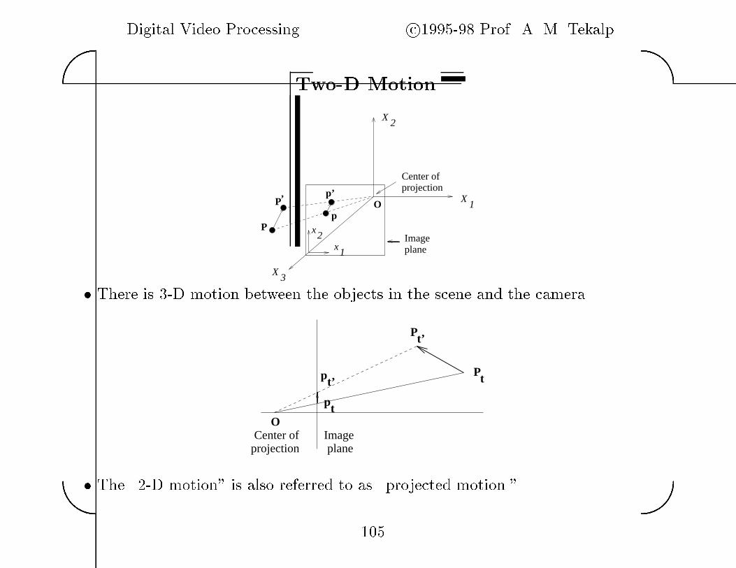
Two�D Motion
O
Pp
Pp’ ’ projection
plane
X1
X2
X3
x2
x1
Center of
Image
� There is ��D motion between the objects in the scene and the camera�
P
P
p
p
Ot
t’ t
t’
projection planeCenter of Image
� The ���D motion� is also referred to as �projected motion��
� �

Digital Video Processing c�������� Prof� A� M� Tekalp��
��
��D Displacement and Velocity Fields
� The ��D displacement �eld is a vector �eld consisting of the x� and x�
components of the frame�to�frame �projected� displacement vectors at each pixel�
ttime
∆ tlttime -
d1
d2
= (x’ , x’ )’P 1 2
= (x’ , x’ )’P 1 2
d1
d2
P = (x , x )1 21 2 = [ d d ]d
∆ tlttime +
T
� The ��D velocity �eld is a vector �eld consisting of the x� and x� components
of the instantaneous velocity vectors at each pixel�
� �

Digital Video Processing c�������� Prof� A� M� Tekalp��
��
Optical Flow and Correspondence Fields
� The observable variations of the ��D image brightness pattern
�the apparent ��D velocity �eld� is called the optical �ow�
� The set of vectors indicating the apparent displacement of pixels from frame to
frame is called the correspondence �eld�
� The optical �ow�correspondence �eld is in general di�erent from the
projected ��D motion �eld due to�
� lack of su�cient spatial image gradient
� changes in external illumination
� changes in shading �due to rotation� etc�
� �
Digital Video Processing c�������� Prof� A� M� Tekalp��
��
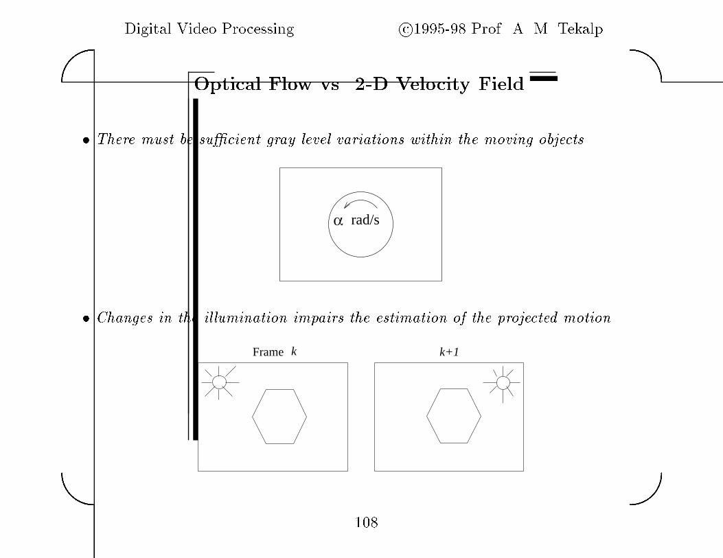
Optical Flow vs� ��D Velocity Field
� There must be su�cient gray level variations within the moving objects�
rad/sα
� Changes in the illumination impairs the estimation of the projected motion�
k k+1Frame � �
Digital Video Processing c�������� Prof� A� M� Tekalp��
��
Optical Flow Estimation
Determination of the apparent velocity v�x�� x�� t� of pixels from a pair of
time�sequential ��D images� The �ow vectors may vary by the coordinates
�space�varying �ow� due to ��D rotation zoom etc�
Correspondence Problem
Finding the apparent displacement vectors d�x�� x�� t� ��t� between a pair of
frames t and t� � t� ��t� Dense or feature correspondence estimation� �May
also appear in the context of stereo disparity estimation��
Image Registration �Special case�
Given two frames that are globally shifted with respect to each other estimate
the shift� There is one displacement vector for a pair of frames�
� �
Digital Video Processing c�������� Prof� A� M� Tekalp��
��
��D Motion�Optical Flow Estimation is Ill�Posed
� Estimation of the optical �ow �or the ��D motion �eld� given two frames
without additional assumptions is �ill�posed��
�� Existence of a solution� No correspondence can be found at occlusion points
�covered�uncovered background problem��
�� Uniqueness of the solution� If the x� and x� coordinates of the displacement
�or velocity� at each pixel is treated as independent variables then the
number of unknowns is twice the number of observations � the elements of
the frame di�erence�
� Theoretically we can determine only motion that is orthogonal to the spatial
image gradient called the normal �ow at any pixel �the aperture problem��
��
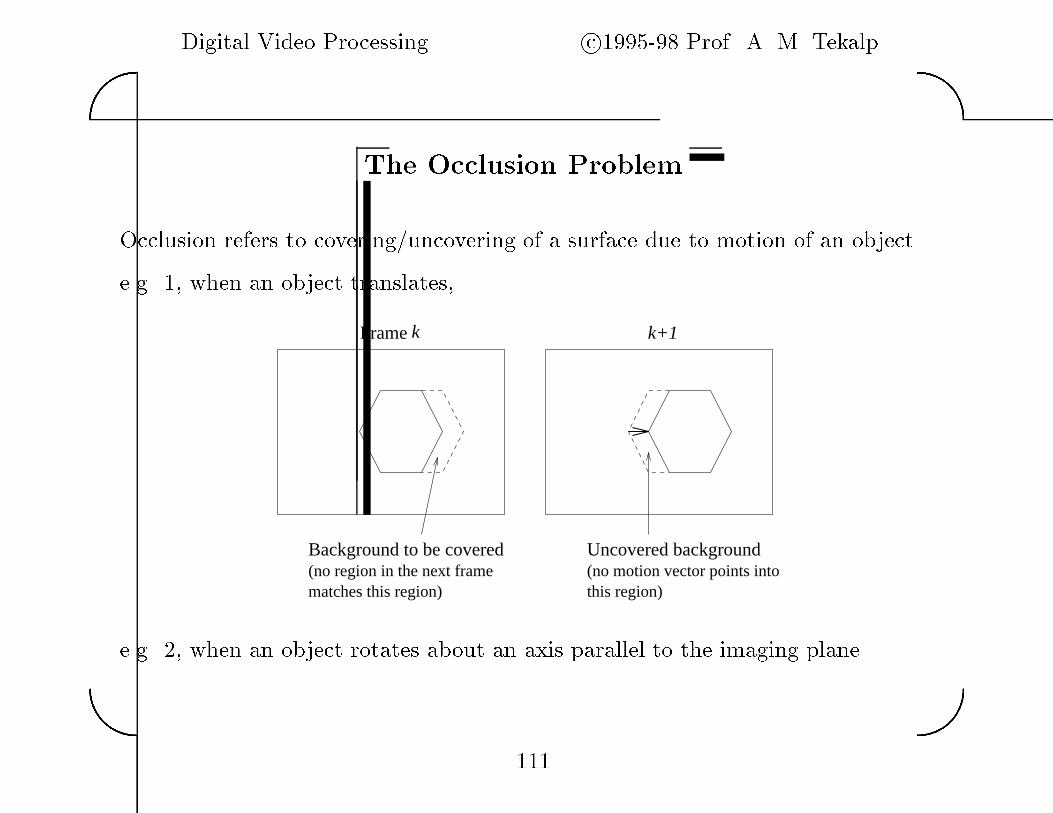
Digital Video Processing c�������� Prof� A� M� Tekalp��
��
The Occlusion Problem
Occlusion refers to covering�uncovering of a surface due to motion of an object�
e�g� � when an object translates
(no region in the next framematches this region)
(no motion vector points intothis region)
k k+1Frame
Background to be covered Uncovered background
e�g� � when an object rotates about an axis parallel to the imaging plane�
���

Digital Video Processing c�������� Prof� A� M� Tekalp��
��
The Aperture Problem
Aperture 1
Aperture 2
flowNormal
� Basic Idea�
We can only observe and determine displacement that is orthogonal to the edges
�in the direction of the intensity gradient�����
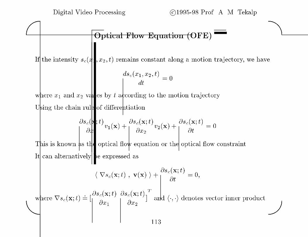
Digital Video Processing c�������� Prof� A� M� Tekalp��
��
Optical Flow Equation �OFE�
If the intensity sc�x�� x�� t� remains constant along a motion trajectory we have
dsc�x�� x�� t�
dt
�
where x� and x� varies by t according to the motion trajectory�
Using the chain rule of di�erentiation
�sc�x� t�
�x�
v��x� ��sc�x� t�
�x�
v��x� ��sc�x� t�
�t
�
This is known as the optical �ow equation or the optical �ow constraint�
It can alternatively be expressed as
h rsc�x� t� � v�x� i��sc�x� t�
�t
� �
where rsc�x� t��� ��sc�x� t�
�x�
�sc�x� t�
�x�
�T
and h�� �i denotes vector inner product�
���
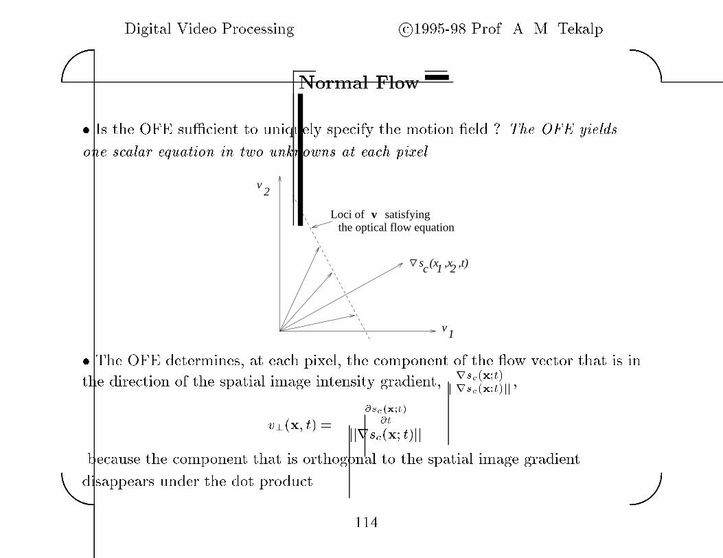
Digital Video Processing c�������� Prof� A� M� Tekalp��
��
Normal Flow
� Is the OFE su�cient to uniquely specify the motion �eld � The OFE yields
one scalar equation in two unknowns at each pixel�
v2
v1
the optical flow equation
cs (x ,x ,t)
v
21
Loci of satisfying
� The OFE determines at each pixel the component of the �ow vector that is in
the direction of the spatial image intensity gradient rsc�x�t�
jjrsc�x�t�jj
v��x� t� � �
�sc�x�t�
�t
jjrsc�x� t�jj
because the component that is orthogonal to the spatial image gradient
disappears under the dot product�
��
Digital Video Processing c�������� Prof� A� M� Tekalp��
��
Motion Models
Because of the ill�posed nature of the problem motion estimation algorithms use
additional assumptions �models� about the structure of the ��D motion �eld�
� Non�parametric models�
Some sort of smoothness or uniformity constraint on the ��D motion �eld�
� Quasi�parametric models�
In ��D rigid motion six egomotion parameters constrain the local �ow vector to
lie along a speci�c line while the local depth value is required to determine its
exact value�
� Parametric models�
��D rigid motion of the image of a planar surface under orthographic projection
can be described by a ��parameter a�ne model while under perspective
projection it can be described by an ��parameter nonlinear model� There exist
more complicated models for quadratic surfaces�
���
Digital Video Processing c�������� Prof� A� M� Tekalp��
��
Nonparametric ��D Motion Estimation Methods
� Methods Based on the OFE� Constant intensity along the motion trajectory
yields an equation in terms of spatio�temporal intensity gradients� Used in
conjunction with appropriate spatio�temporal smoothness constraints�
� Phase�Correlation Method� The linear term of the Fourier phase di�erence
between the consecutive frames determines the motion estimates�
� Block Matching Method� Matching �xed size blocks between two frames
based on a distance criterion� Extension to feature matching �e�g� edges
corners��
� Pel�Recursive Methods� Gradient�based minimization of the displaced frame
di�erence� Implicit use of smoothness constraint� Extension to Wiener�type
motion estimation�
� Bayesian Methods� Probabilistic smoothness constraint in the form of Gibbs
random �elds�
���
Digital Video Processing c�������� Prof� A� M� Tekalp��
��
Methods using the OFE
� COLOR IMAGES
OFE can be imposed at each color band separately� Thus the displacement
vector is e�ectively constrained in three di�erent directions since the
direction of the spatial gradient vector at each band is di�erent in general�
� MONOCHROMATIC IMAGES
The solution space for the displacement vector can be reduced by using an
appropriate smoothness constraint which requires the displacement vector to
vary slowly over a neighborhood�
���
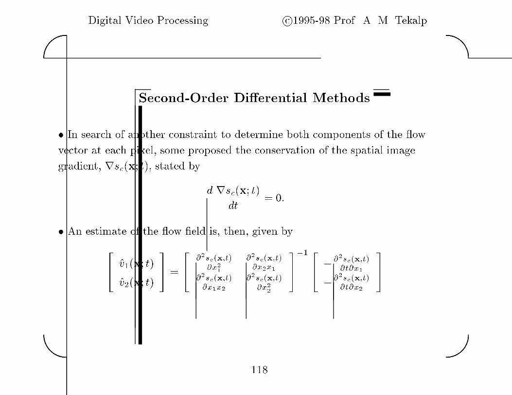
Digital Video Processing c�������� Prof� A� M� Tekalp��
��
Second�Order Di�erential Methods
� In search of another constraint to determine both components of the �ow
vector at each pixel some proposed the conservation of the spatial image
gradient rsc�x� t� stated byd rsc�x� t�
dt
� �
� An estimate of the �ow �eld is then given by
�� �v��x� t�
�v��x� t��
� ��
� ��sc�x�t�
�x��
��sc�x�t�
�x�x�
��sc�x�t�
�x�x�
��sc�x�t�
�x��
��
�� �� ���sc�x�t�
�t�x�
���sc�x�t�
�t�x�
��
���
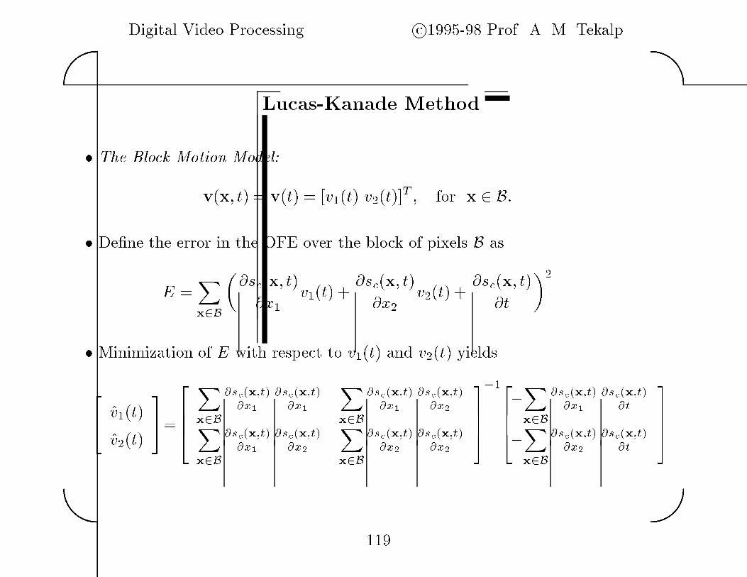
Digital Video Processing c�������� Prof� A� M� Tekalp��
��
Lucas�Kanade Method
� The Block Motion Model�
v�x� t� � v�t� � �v��t� v��t��T � for x � B�
� De�ne the error in the OFE over the block of pixels B as
E �X
x�B�
�sc�x� t�
�x�
v��t� ��sc�x� t�
�x�
v��t� ��sc�x� t�
�t
��
� Minimization of E with respect to v��t� and v��t� yields
�� �v��t�
�v��t��
���
���X
x�B�sc�x�t�
�x�
�sc�x�t�
�x�
Xx�B
�sc�x�t�
�x�
�sc�x�t�
�x�Xx�B
�sc�x�t�
�x�
�sc�x�t�
�x�
Xx�B
�sc�x�t�
�x�
�sc�x�t�
�x�
����
�������X
x�B�sc�x�t�
�x�
�sc�x�t�
�t
�X
x�B�sc�x�t�
�x�
�sc�x�t�
�t
����
���

Digital Video Processing c�������� Prof� A� M� Tekalp��
��
Horn�Schunck Method
Minimize a weighted sum of the error in the OFE and a measure of departure
from smoothness in the motion �eld
minv�x�E �Z
��E�of �v� � c�E�s �v��dx
to estimate the velocity vector at each pixel where denotes the image support
and
Eof �v�x�� � h rg�x� t� � v�x� i��g�x� t�
�t
�
and
E�s �v�x�� � jjrv��x�jj� � jjrv��x�jj�
� ��v�
�x��� � ��v�
�x��� � ��v�
�x��� � ��v�
�x����
The parameter c� �chosen heuristically� is a weight that controls the strength of
the smoothness constraint� Larger values of c� increase the strength of the
constraint whereas smaller values relax the constraint�
��

Digital Video Processing c�������� Prof� A� M� Tekalp��
��
� The minimization of the functional E using the calculus of variations and
approximation of the Laplacian of the velocity components by linear highpass
�lters yields the following iterations�
v�n���
� �x� t� � !v�n�
� �x� t���sc
�x��sc
�x�!v�n�
� �x� t� � �sc
�x�!v�n�
� �x� t� � �sc�t
�� � � �sc�x��� � � �sc�x���
v�n���
� �x� t� � !v�n�
� �x� t���sc
�x��sc
�x�!v�n�
� �x� t� � �sc
�x�!v�n�
� �x� t� � �sc�t
�� � � �sc�x��� � � �sc�x���
where all partials are evaluated at the point �x� t�� The initial estimates of the
velocities v���
� �x� t� and v���
� �x� t� can be obtained by the block matching
technique�
� In the digital implementation of the algorithm the derivatives are numerically
estimated�
���
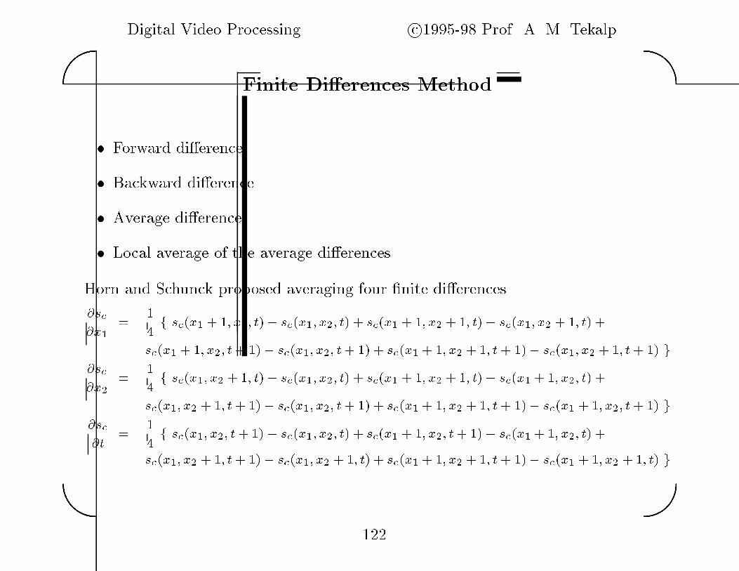
Digital Video Processing c�������� Prof� A� M� Tekalp��
��
Finite Di�erences Method
� Forward di�erence
� Backward di�erence
� Average di�erence
� Local average of the average di�erences
Horn and Schunck proposed averaging four �nite di�erences
�sc
�x�
�
��f sc�x� � �� x�� t�� sc�x�� x�� t� � sc�x� � �� x� � �� t�� sc�x�� x� � �� t� �
sc�x� � �� x�� t� ��� sc�x�� x�� t� �� � sc�x� � �� x� � �� t� ��� sc�x�� x� � �� t� �� g
�sc
�x�
�
��f sc�x�� x� � �� t�� sc�x�� x�� t� � sc�x� � �� x� � �� t�� sc�x� � �� x�� t� �
sc�x�� x� � �� t� ��� sc�x�� x�� t� �� � sc�x� � �� x� � �� t� ��� sc�x� � �� x�� t� �� g
�sc�t
�
��f sc�x�� x�� t� ��� sc�x�� x�� t� � sc�x� � �� x�� t� ��� sc�x� � �� x�� t� �
sc�x�� x� � �� t� ��� sc�x�� x� � �� t� � sc�x� � �� x� � �� t� ��� sc�x� � �� x� � �� t� g
���

Digital Video Processing c�������� Prof� A� M� Tekalp��
��
Local Polynomial Fitting Method
Approximate sc�x�� x�� t� locally by a linear combination of some low order
polynomials in x� x� and t i�e�
�sc�x�� x�� t� �N��X
i�ai�i�x�� x�� t�
where N is the number of the basis polynomials ai are the coe�cients of the
linear superposition and �i�x�� x�� t� are the basis polynomials�
Set N � � with the following basis functions
�i�x�� x�� t� � �� x�� x�� t� x�
�� x�
�� x�x�� x�t� x�t
Then
�sc�x�� x�� t� � a�� � a�x� � a�x� � at� a�x�
� �
a�x�
� � a x�x� � a�x�t� a�x�t�
���

Digital Video Processing c�������� Prof� A� M� Tekalp��
��
The coe�cients ai i � ���� are estimated by using the least squares method
which minimizes the error function
e� �X
n�
Xn�
Xn��sc�x�� x�� t��
N��Xi�
ai�i�x�� x�� t���jx�n��x�yn��x�tn��t
with respect to these coe�cients�
The summation is over a local neighborhood of the pixel� A typical case involves
� pixels �x� spatial windows in two consecutive frames�
Once the coe�cients ai are estimated image gradients can be found by simple
di�erentiation�sc�x�� x�� t�
�x�
� a� � �a�x� � a x� � a�tjx�x�t� � a�
�sc�x�� x�� t�
�x�
� a� � �a�x� � a x� � a�tjx�x�t� � a�
�sc�x�� x�� t�
�t
� a � a�x� � a�x�jx�x�t� � a
Estimating the coe�cients of the �rst three basis polynomials is su�cient to
estimate the gradients�
��
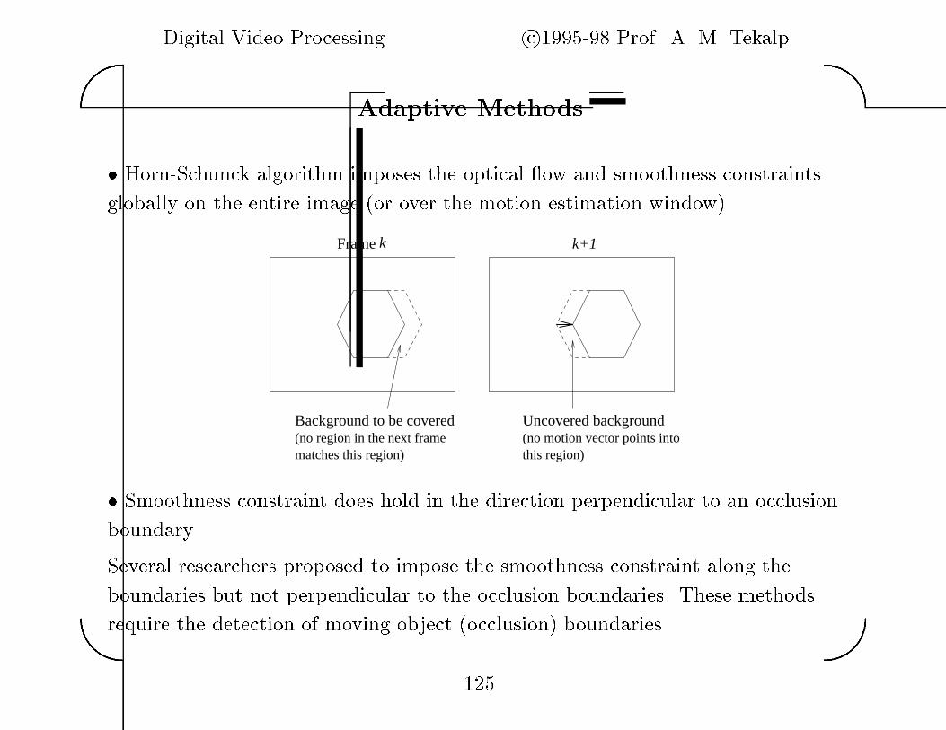
Digital Video Processing c�������� Prof� A� M� Tekalp��
��
Adaptive Methods
� Horn�Schunck algorithm imposes the optical �ow and smoothness constraints
globally on the entire image �or over the motion estimation window��
(no region in the next framematches this region)
(no motion vector points intothis region)
k k+1Frame
Background to be covered Uncovered background
� Smoothness constraint does hold in the direction perpendicular to an occlusion
boundary�
Several researchers proposed to impose the smoothness constraint along the
boundaries but not perpendicular to the occlusion boundaries� These methods
require the detection of moving object �occlusion� boundaries�
���

Digital Video Processing c�������� Prof� A� M� Tekalp��
��
LECTURE �
BLOCK�BASED METHODS
�� Phase�Correlation Method
�� Block�Matching Algorithms
� Full�Search
� Three�Step Algorithm
� Cross�Search Algorithm
�� Hierarchical Motion Estimation
� Motion Estimation with Spatial Transformations
� Generalized Block�Matching
� Extension of Lucas�Kanade Method
��

Digital Video Processing c�������� Prof� A� M� Tekalp��
��
Block Translation Model
Assume frame k � � is a globally �at least on a block�by�block basis shifted
version of frame ks�n�� n�� k � � � s�n� � d�� n� � d�� k
� To overcome the aperture problem� there must be su�cient gray level
variation within the block�
� This model is used in many practical applications including
� World standards for video compression such as H��� and MPEG
� Motion�compensated �ltering in standards conversion� etc���
���
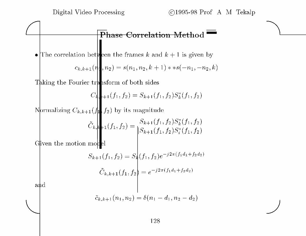
Digital Video Processing c�������� Prof� A� M� Tekalp��
��
Phase Correlation Method
� The correlation between the frames k and k � � is given by
ck�k���n�� n� � s�n�� n�� k � � � �s��n���n�� k
Taking the Fourier transform of both sides
Ck�k���f�� f� � Sk���f�� f� S�
k�f�� f�
Normalizing Ck�k���f�� f� by its magnitude
�Ck�k���f�� f� �
Sk���f�� f� S�k�f�� f�
jSk���f�� f� S�i �f�� f� j
Given the motion model
Sk���f�� f� � Sk�f�� f� e�j���f�d��f�d��
�Ck�k���f�� f� � e�j���f�d��f�d��
and
�ck�k���n�� n� � ��n� � d�� n� � d�
���
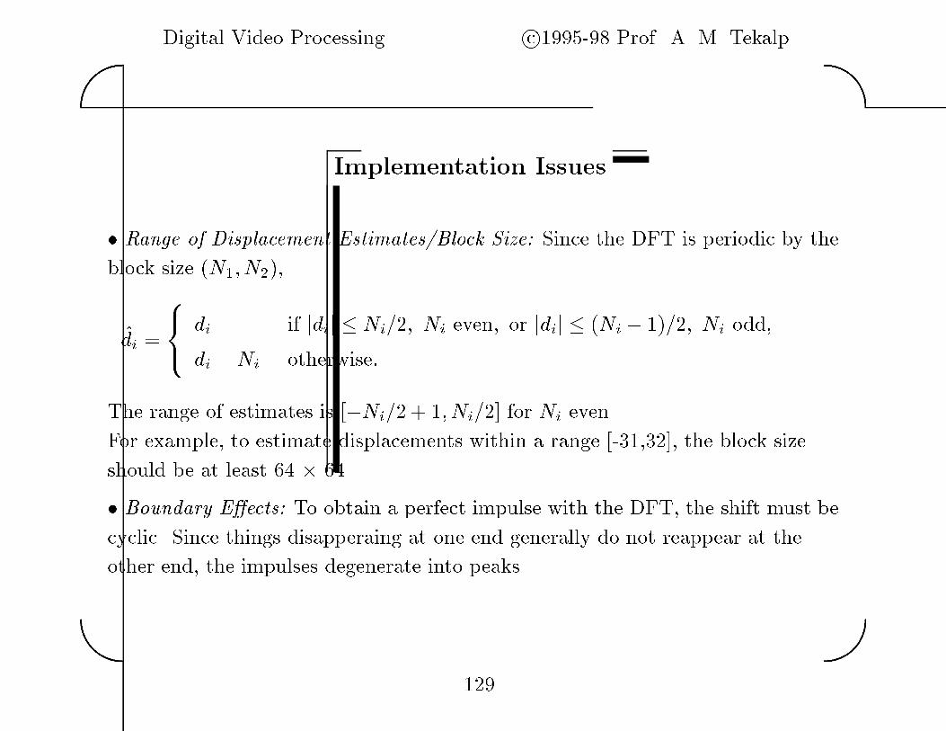
Digital Video Processing c�������� Prof� A� M� Tekalp��
��
Implementation Issues
� Range of Displacement Estimates�Block Size� Since the DFT is periodic by the
block size �N�� N� �
�di ���
�di if jdij � Ni��� Ni even� or jdij � �Ni � � ��� Ni odd�
di �Ni otherwise�
The range of estimates is ��Ni�� � �� Ni��� for Ni even�
For example� to estimate displacements within a range ��������� the block size
should be at least � �
� Boundary E�ects� To obtain a perfect impulse with the DFT� the shift must be
cyclic� Since things disapperaing at one end generally do not reappear at the
other end� the impulses degenerate into peaks�
���

Digital Video Processing c�������� Prof� A� M� Tekalp��
��
Comments on Phase Correlation
� Multiple Moving Objects� Experiments indicate that multiple peaks are
observed in such a case� An additional search is required to �nd which peak
belongs to which part of the image�
� Frame�to�Frame Intensity Changes� Shifts in the mean value or
multiplication by a constant do not a�ect the Fourier phase� The method is
insensitive to such changes�
� Extension to include rotation is possible �although costly �
���

Digital Video Processing c�������� Prof� A� M� Tekalp��
��
Block Matching Method
� The displacement at the center of an N� �N� block in frame k is determined
by searching for the location of the best matching block of the same size in
the frame k � �� The search is limited to within a search window�
Frame
k+1
Search window
Block
k
� Block matching algorithms di�er in
� Matching criteria �maximum cross�correlation� minimum error
� Search strategy
� Determination of block size �hierarchical� adaptive
���
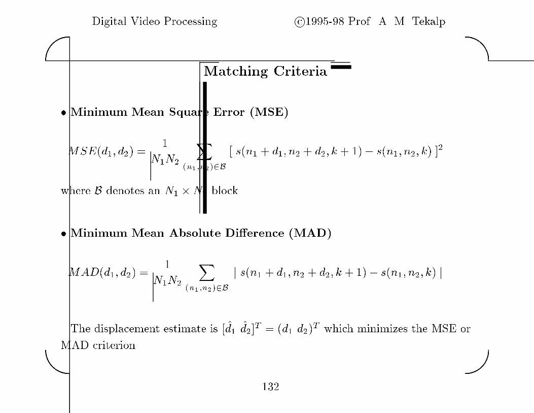
Digital Video Processing c�������� Prof� A� M� Tekalp��
��
Matching Criteria
� Minimum Mean Square Error �MSE�
MSE�d�� d� �
�N�N�
X�n��n���B
� s�n� � d�� n� � d�� k � � � s�n�� n�� k ��
where B denotes an N� �N� block�
� Minimum Mean Absolute Di�erence �MAD�
MAD�d�� d� �
�N�N�
X�n��n���B
j s�n� � d�� n� � d�� k � � � s�n�� n�� k j
� The displacement estimate is � �d� �d��T � �d� d� T which minimizes the MSE or
MAD criterion�
���
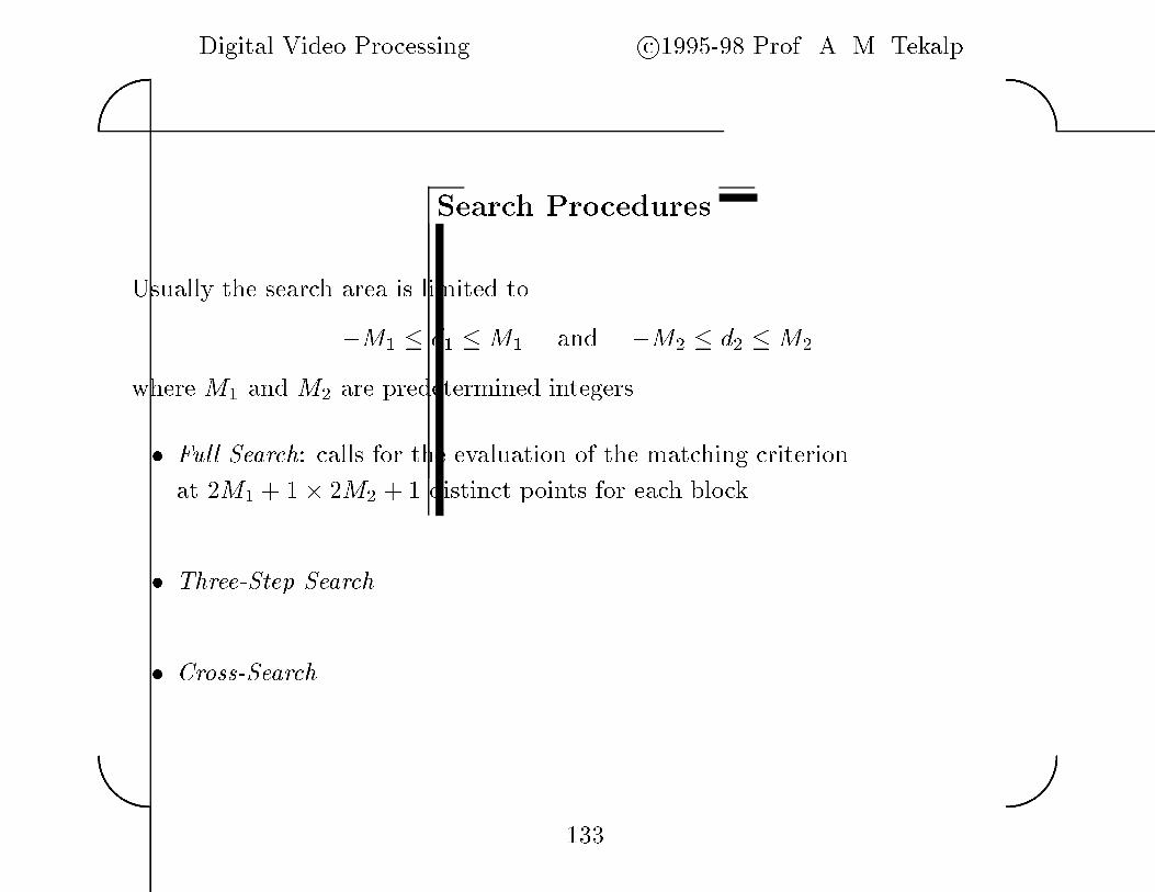
Digital Video Processing c�������� Prof� A� M� Tekalp��
��
Search Procedures
Usually the search area is limited to
�M� � d� �M� and �M� � d� �M�
where M� and M� are predetermined integers�
� Full Search� calls for the evaluation of the matching criterion
at �M� � �� �M� � � distinct points for each block�
� Three�Step Search
� Cross�Search
���
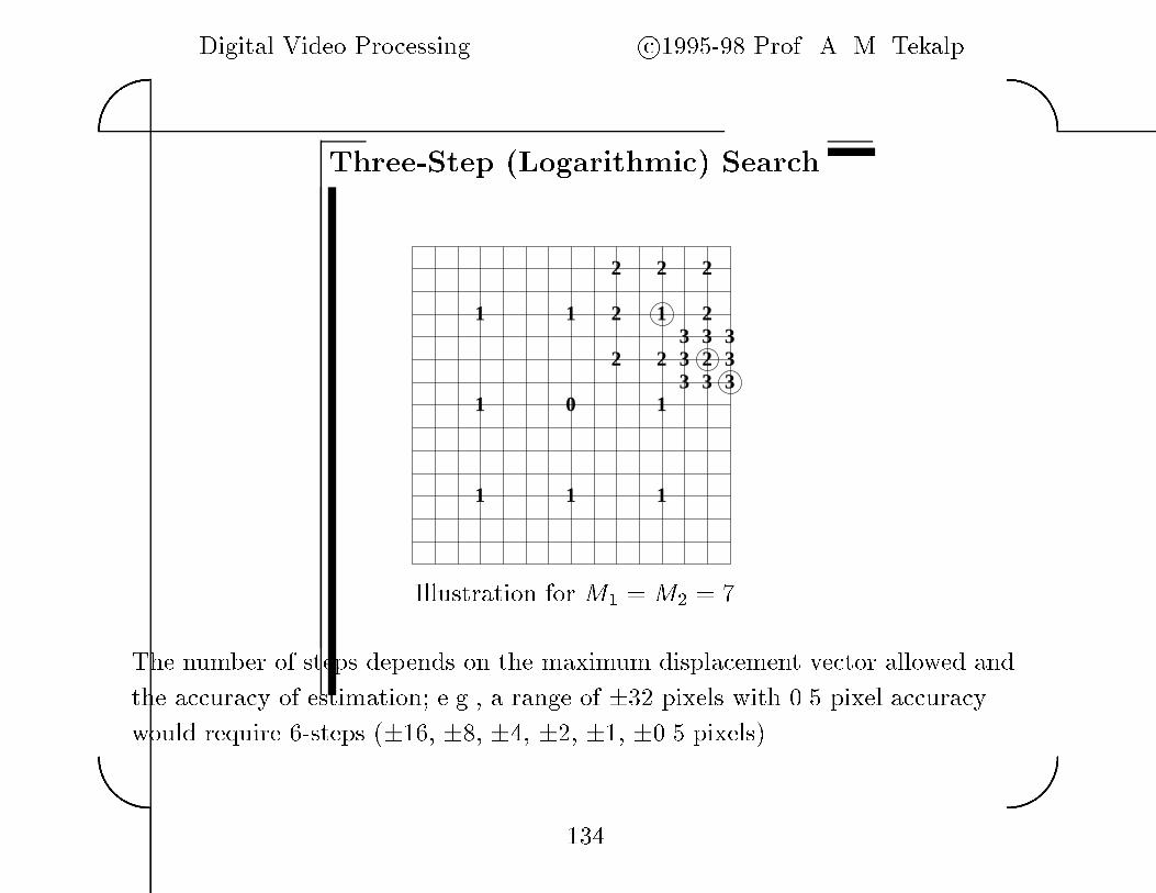
Digital Video Processing c�������� Prof� A� M� Tekalp��
��
Three�Step �Logarithmic� Search
0 1
111
1 1
1
1
2
2 2 2
2
22233333
33 3
Illustration for M� �M� � ��
The number of steps depends on the maximum displacement vector allowed and
the accuracy of estimation� e�g�� a range of ��� pixels with ��� pixel accuracy
would require �steps ���� ��� �� ��� ��� ���� pixels �
��
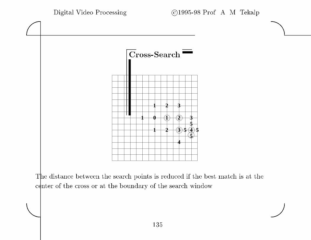
Digital Video Processing c�������� Prof� A� M� Tekalp��
��
Cross�Search
0 11
1
1
2
2
2
3
3
3 4
4
55
55
The distance between the search points is reduced if the best match is at the
center of the cross or at the boundary of the search window�
���

Digital Video Processing c�������� Prof� A� M� Tekalp��
��
Comments on Block Matching
� Minimizing the MSE or MAD criteria can be viewed as imposing the optical
�ow constraint on the entire block�
� It is assumed that all pixels belonging to a block have a single translation
vector� which is a special case of the local smoothness constraint �same as in
Lucas�Kanade method �
� Block size selection� There are con�icting requirements on the size of the
blocks�� The block size should be su�ciently large� It is possible that a match
may be established between blocks containing similar gray�level patterns
which are unrelated in the motion sense�
� The block size should be su�ciently small� If the motion vector varies
within a block� block matching cannot provide accurate estimates�
��

Digital Video Processing c�������� Prof� A� M� Tekalp��
��
Hierarchical Image Representation
� A hierarchical representation of the image sequence is formed using a simple
low pass �ltering operation at each level�
Increasingresolution
Level 3
Level 2
Level 1
Decimation at each layer is optional�
���

Digital Video Processing c�������� Prof� A� M� Tekalp��
��
Hierarchical Block Matching
� Perform block matching at each level starting with the lowest resolution
image �highest level � Interpolate the result and pass onto the next higher
resolution image as an initial estimate�
� The lower resolution levels serve to determine a rough estimate of the
displacement using larger blocks�
� The higher resolution levels serve to �ne�tune the displacement vector
estimate� At higher resolution levels� smaller window size can be used since
we start with a relatively good initial estimate�
���
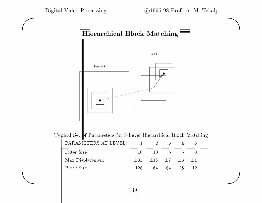
Digital Video Processing c�������� Prof� A� M� Tekalp��
��
Hierarchical Block Matching
k+1
kFrame
Typical Set of Parameters for ��Level Hierarchical Block Matching
PARAMETERS AT LEVEL� � � � � �
Filter Size �� �� � � �
Max Displacement ��� ��� �� �� ��
Block Size �� � � � ��
���

Digital Video Processing c�������� Prof� A� M� Tekalp��
��
Hierarchical BM � An Example
The center of the search area in the second level �denoted by ��� denotes the
estimate from the �rst level�0 1
111
1 1
1
1
2
2 2 2
2
22233333
33 3
0
1 1 1
1
111
1
22 2
2222
2
Level 2 (lower resolution)
Level 1 (higher resolution)
M � � ���steps for level � and M � � ���steps for level ��
The estimates in the �st and �nd levels are ��� ��T and ��� ��T � respectively�
resulting in an estimate of ���� ��T �
��

Digital Video Processing c�������� Prof� A� M� Tekalp��
��
Shortcomings of Block Matching
Translational motion ���parameter �frame k frame k+1
� cannot handle rotation or zooming�
Accuracy is essential in motion�compensated �ltering�
� discontinuity at block boundaries�
Blocking artifacts in motion�compensated compression�
��
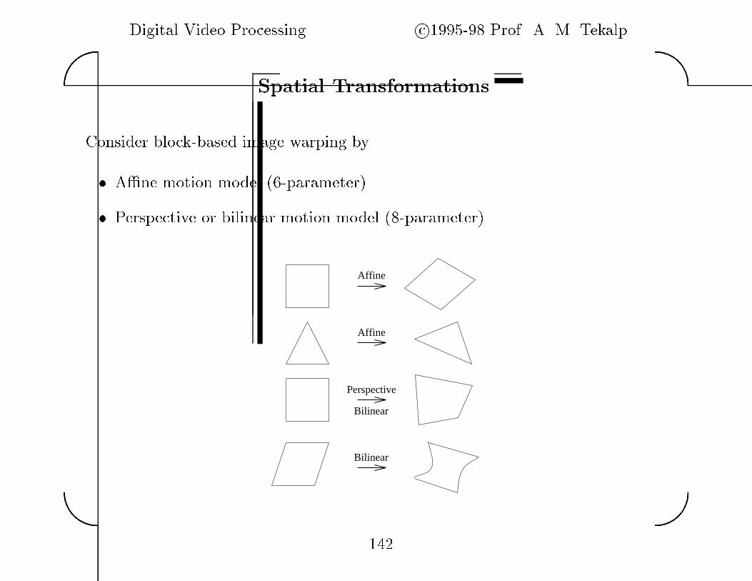
Digital Video Processing c�������� Prof� A� M� Tekalp��
��
Spatial Transformations
Consider block�based image warping by
� A�ne motion model ��parameter �
� Perspective or bilinear motion model ���parameter �
Affine
Affine
Perspective
Bilinear
Bilinear
��
Digital Video Processing c�������� Prof� A� M� Tekalp��
��
Motion Estimation with Spatial Transformations
� Generalized block matching
� Search method �Seferidis and Ghanbari
� Algebraic method �Extension of Lucas�Kanade method
� ��D mesh modeling �motion continuity across block boundaries
� Hexagonal search �Nakaya et al�
� Constrained linear estimation �Altunbasak and Tekalp
��

Digital Video Processing c�������� Prof� A� M� Tekalp��
��
Generalized Block Matching
Frame k-1 Frame k
Texture mapping
� Search for all combinations of the coordinates of the corners to minimize the
SAD�
... . ... . .
... . ... . . ... . ..
. . .
... . ... . .
reference frame current frame
�
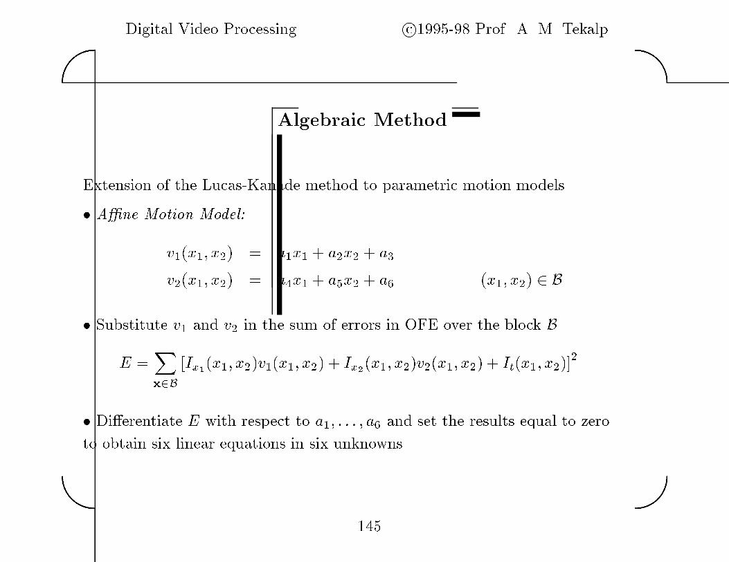
Digital Video Processing c�������� Prof� A� M� Tekalp��
��
Algebraic Method
Extension of the Lucas�Kanade method to parametric motion models�
� A�ne Motion Model�
v��x�� x� � a�x� � a�x� � a�
v��x�� x� � a�x� � a�x� � a �x�� x� � B
� Substitute v� and v� in the sum of errors in OFE over the block B
E �X
x�B
�Ix��x�� x� v��x�� x� � Ix��x�� x� v��x�� x� � It�x�� x� ��
� Di�erentiate E with respect to a�� � � � � a and set the results equal to zero
to obtain six linear equations in six unknowns
��

Digital Video Processing c�������� Prof� A� M� Tekalp��
��
Extension of Lucas�Kanade Method �cont�d�
����
�a��a�
�a��a�
�a��a�
��� �
������
PI�
x�
Px�I�
x�
Px�I�
x�
PIx�
Ix�
Px�Ix�
Ix�
Px�Ix�
Ix�Px�I�
x�
Px�
�I�
x�
Px�x�I�
x�
Px�Ix�
Ix�
Px�
�Ix�
Ix�
Px�x�Ix�
Ix�Px�I�
x�
Px�x�I�
x�
Px�
�I�
x�
Px�Ix�
Ix�
Px�x�Ix�
Ix�
Px�
�Ix�
Ix�PIx�
Ix�
Px�Ix�
Ix�
Px�Ix�
Ix�
PI�
x�
Px�I�
x�
Px�I�
x�Px�Ix�
Ix�
Px�
�Ix�
Ix�
Px�x�Ix�
Ix�
Px�I�
x�
Px�
�I�
x�
Px�x�I�
x�Px�Ix�
Ix�
Px�x�Ix�
Ix�
Px�
�Ix�
Ix�
Px�I�
x�
Px�x�I�
x�
Px�
�I�
x�
�����
��
������
�
PIx�
It
�
Px�Ix�
It
�
Px�Ix�
It
�
PIx�
It
�
Px�Ix�
It
�
Px�Ix�
It
�����
�
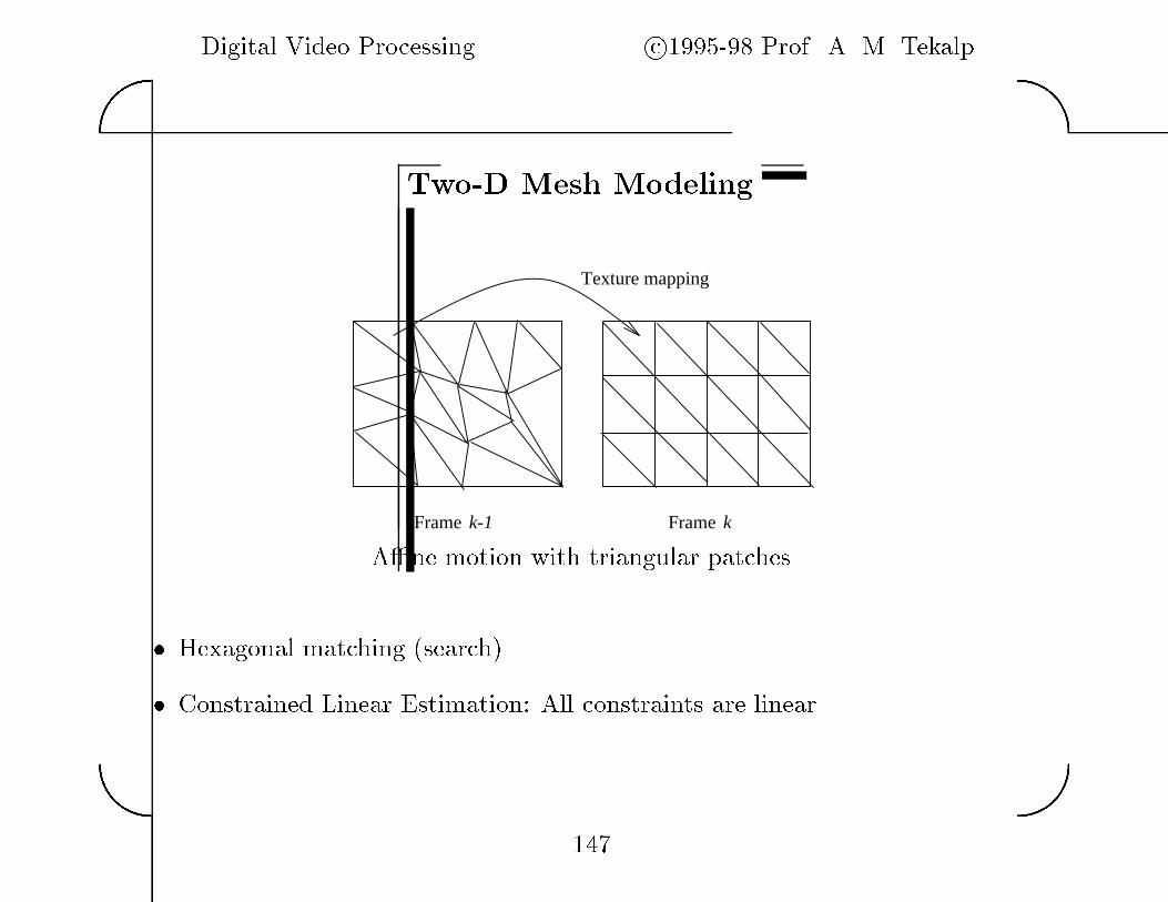
Digital Video Processing c�������� Prof� A� M� Tekalp��
��
Two�D Mesh Modeling
Frame k-1 Frame k
Texture mapping
A�ne motion with triangular patches�
� Hexagonal matching �search �
� Constrained Linear Estimation� All constraints are linear�
��

Digital Video Processing c�������� Prof� A� M� Tekalp��
��
Hexagonal Matching
x
� There are six lines intersecting at each node in the case of a uniform
triangular mesh�
� The boundaries of these six triangles de�ne a hexagon�
� Perturb each node point to yield the smallest SAD within its hexagon�
��
Digital Video Processing c�������� Prof� A� M� Tekalp��
��
LECTURE �
PEL RECURSIVE METHODS
�� Minimization by Gradient Descent
�� Netravali�Robbins Algorithm
�� Walker�Rao Algorithm
� Wiener�based Estimation��
Digital Video Processing c�������� Prof� A� M� Tekalp��
��
Displaced Frame Di�erence �DFD�
Let
dx� t��t �
� �d�x� t��t d�x� t��t �T
denote the displacement �eld at x�
� �x� x��T between frames t and t��t�
The DFD function between these two frames is de�ned as
dfdx� �d �
� scx� �dx� t� �t � t��t � scx� t �
where sc� denotes the spatio�temporal image intensity distribution�
� If the components of �d take noninteger values� interpolation is required to
compute dfd at each pixel location�
� If �d is equal to the true displacement vector and there is no interpolation
errors� dfd attains the value of zero at that pixel location�
���

Digital Video Processing c�������� Prof� A� M� Tekalp��
��
Relation between DFD and OFE
� Expanding the dfd into Taylor series about x� t � for dx and �t small�
scx� � d�x � x� � d�x � t��t � scx� t � d�x �scx� t
�x�
�d�x �scx� t
�x�
��t�scx� t
�t
� h�o�t�
� Neglecting h�o�t�� and setting dfdx� �d � �� we obtain
�scx� t
�x�
�d�x ��scx� t
�x�
�d�x � �t�scx� t
�t
� ��
� Dividing both sides by �t� and taking the limit �t� �
�scx� t
�x�
�v�x ��scx� t
�x�
�v�x ��scx� t
�t
� ��
���

Digital Video Processing c�������� Prof� A� M� Tekalp��
��
Comments
� In the case of constant velocity motion� where
d�x � v�x �t and d�x � v�x �t�
the optical �ow equation is satis�ed when the displaced frame di�erence function
attains the value of zero�
� In practice� neither the dfd nor the error in the OFE is exactly zero� because
� there is observation noise�
� scene illumination may vary by time�
� there are occlusion regions� and
� there are interpolation errors�
� Therefore� one aims to minimize the absolute value or the square of the dfd or
the LHS of the OFE to obtain an estimate of the frame�to�frame motion �eld�
���
Digital Video Processing c�������� Prof� A� M� Tekalp��
��
PEL�RECURSIVE ALGORITHMS
Pel�recursive algorithms are of the general form
di��x � dix � uix
where dix is the estimated motion vector at the pel location x in the ith
step� uix is the update term in the ith step� and di��x is the new estimate�
� The update term uix is estimated� at each pel x� to minimize a
positive�de�nite function E of the dfd with respect to d�
� The iterations may be executed at a single pel pixel position
or at consecutive pel positions or a combination of both�
The motion estimate at the previous pel is taken as the initial estimate at the
next pel� hence pel�recursive�
���

Digital Video Processing c�������� Prof� A� M� Tekalp��
��
Minimization by Gradient Descent
A straightforward way to minimize a function is to set its derivatives to zero�
rdEx�d � �
where rd is the gradient operator with respect to d� the set of partial derivatives�
The following equations must be solved simultaneously�
�Ex�d
�d�
� �
�Ex�d
�d�
� �
Since an analytical solution to these equations cannot be found in general� we
resort to iterative methods�
��
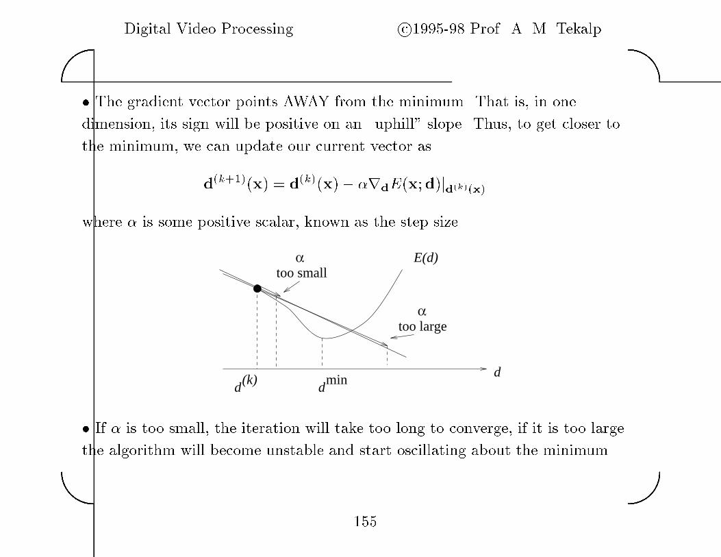
Digital Video Processing c�������� Prof� A� M� Tekalp��
��
� The gradient vector points AWAY from the minimum� That is� in one
dimension� its sign will be positive on an �uphill� slope� Thus� to get closer to
the minimum� we can update our current vector as
d�k���x � d�k�x � �rdEx�d jd�k��x�
where � is some positive scalar� known as the step size�
α
αtoo small
too large
E(d)
dmin
d(k)
d
� If � is too small� the iteration will take too long to converge� if it is too large
the algorithm will become unstable and start oscillating about the minimum�
���

Digital Video Processing c�������� Prof� A� M� Tekalp��
��
Newton�Raphson Method
� We can estimate a good value for � using the well�known Newton�Raphson
method for root �nding
d�k���x � d�k�x �H��rdEx�d jd�k��x�
where H is the Hessian matrixHij ��
��Ex�d
�di�dj�
� In one dimension� we would like to �nd a root of E�
d �
Expanding E�
d in a Taylor series about the point d�k�
E�
d�k��� � E�
d�k� � d�k��� � d�k� E��
d�k�
Since we want d�k��� to be a zero of E�
� we set
E�
d�k� � d�k��� � d�k� E��
d�k� � �
Thus�
d�k��� � d�k� �E
�d�k�
E��d�k�
���
Digital Video Processing c�������� Prof� A� M� Tekalp��
��
Local vs� Global Minima
� Gradient descent su�ers from a serious problem� its solution is strongly
dependent on the starting point� If start in a �valley�� it will be stuck at the
bottom of that valley� This may be a �local� minimum� We have no way of
getting out of that local minimum to reach the �global� minimum�
� More sophisticated optimization methods� such as simulated
annealing� are needed to be able to reach the global minimum
regardless of the starting point� However� these more sophisticated optimization
methods usually require a lot more processing time�
���
Digital Video Processing c�������� Prof� A� M� Tekalp��
��
Netravali�Robbins Algorithm
The Netravali�Robbins algorithm �nds an estimate of the displacement vector at
each pixel to minimize
Ex�d � �dfdx�d ��
A steepest descent approach to the minimization problem yields the iteration
di��x � dix � ��� � rd�dfdx�di ��
� dix � � dfdx�di rddfdx�di �
where r is the gradient with respect to d�
Since
rddfdx�di � rxscx� di� t��t
the estimate becomes
di��x � dix � � dfdx�di rxscx� di� t��t �
���

Digital Video Processing c�������� Prof� A� M� Tekalp��
��
Walker and Rao Algorithm
Walker and Rao suggested the following step size
� �
�
jjrxscx� di� t��t jj��
This is motivated by the update term
� should be large when jdfd� j is large and jrsc� j is small� and
� should be small when jdfd� j is small and jrsc� j is large�
Ca�ario and Rocca have added a bias term �� to avoid division by zero in the
areas of constant intensity
� �
�
jjrxscx� di� t��t jj� � ���
���
Digital Video Processing c�������� Prof� A� M� Tekalp��
��
Extension to Multiple Pixel Support
If we assume that the displacement remains constant over a support M
containing several pixels� we can minimize the dfd over the support M as
opposed to on a pixel�by�pixel basis
EMdM �X
x�M
�dfdx�dM ��
This results in the following estimator
di��
M � diM � ��� � rd
Xx�M
�dfdx�di ���
where di��
M denotes the new displacement estimate over the entire support M �
���

Digital Video Processing c�������� Prof� A� M� Tekalp��
��
Wiener�based Estimation Algorithm
� Linear minimum mean square error LMMSE estimation of the update term
ui based on a neighborhood M of a pel� Extension of the multiple pel version of
Netravali�Robbins algorithm�
Linearization of the dfd at the pels of the support
dfdx� �di � �rTscx� � di� t��t ui � vx� �di
dfdx� �di � �rTscx� � di� t��t ui � vx� �di
��� �
���
dfdxN �di � �rTscxN � di� t��t ui � vxN �di
Expressing this set of equations asz � �uM � v
the LMMSE estimate of the update term is given by
�uM � ��TR��v ��R��u ����TR��v z
where �uM denotes the update term for the entire support M �
���

Digital Video Processing c�������� Prof� A� M� Tekalp��
��
The solution requires the knowledge of the covariance matrices of both the
update Ru and the linearization error Rv�
Assuming that Ru � �uI and Rv � �vI�
�uM � ��T���v
�u����Tz
and
di��
M � diM � ��T���v
�u����Tz
Note that the assumptions that are used to arrive at the simpli�ed estimator are
not in general true� e�g�� the linearization error is not uncorrelated with the
update term� and the updates and the linearization errors at each pixel are not
uncorrelated with each other�
However� experimental results indicate better performance than other
pel�recursive estimators�
���
Digital Video Processing c�������� Prof� A� M� Tekalp��
��
Remarks on Pel�Recursive Methods
� The �pel�recursive� nature of the algorithm can be considered as an implicit
smoothness constraint� The e�ectiveness of this constraint increases especially
when a small number of iterations are performed at each pixel�
� The aperture problem also exists in pel�recursive algorithms� The update term
is a vector along the direction of the gradient of the image intensity� Thus� no
correction is performed in the direction perpendicular to the gradient vector�
� Pel�recursive algorithms can be applied hierarchically� using multi�resolution
representation of images� for improved motion estimation�
���

Digital Video Processing c�������� Prof� A� M� Tekalp��
��
LECTURE �
BAYESIAN METHODS
�� Introduction to Markov Random Fields and Gibbs Distribution
�� Optimization Methods
� Simulated Annealing �SA
� Metropolis algorithm and Gibbs sampler
� Iterated conditional modes �ICM
� Mean eld Annealing �MFA
�� MAP Motion Estimation
� Basic Formulation
� Discontinuity Models
� Estimation Algorithms
��

Digital Video Processing c�������� Prof� A� M� Tekalp��
��
MARKOV AND GIBBS RANDOM FIELDS
� MRFs are extensions of ��D causal Markov chains to ��D�
� MRFs were traditionally specied by local conditional probabilities which
limited their usage� Recently it has been shown that every MRF can be
described by a Gibbs distribution � hence the Gibbs random eld �GRF�
� Bayesian estimation methods can be developed using GRFs as a priori signal
models for complex image processing applications such as motion estimation
and segmentation�
� Since Bayesian estimation requires global optimization of a cost function� we
study a number of optimization methods including simulated annealing �SA�
iterative conditional mode �ICM� and highest con�dence �rst �HCF�
���

Digital Video Processing c�������� Prof� A� M� Tekalp��
��
De�nitions
� Let a random eld z � fz�x�x � �g be specied over a lattice ��
and � � � denote a realization of the random eld z�
The random eld z�x can be continuous or discrete�valued� that is ��x � R
or ��x � � � f�� �� � � � � L� �g� for all x � �� respectively�
� A neighborhood system on ��
The set Nx denotes the neighborhood of the site x� and has the properties�
�i x �� Nx� and
�ii xj � Nxi
� xi � Nxj�
where xi and xj denote arbitrary sites in the lattice�
�In words� x does not belong to its own set of neighbors� and if xj is a neighbor
of xi� then xi is a neighbor of xj� and vice versa�
The neighborhood system over � is then dened as N � fNx�x � �g
���
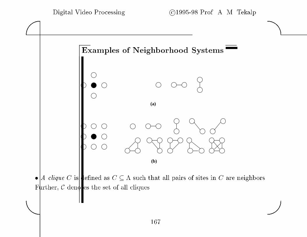
Digital Video Processing c�������� Prof� A� M� Tekalp��
��
Examples of Neighborhood Systems
(b)
(a)
� A clique C is dened as C � � such that all pairs of sites in C are neighbors�
Further� C denotes the set of all cliques����

Digital Video Processing c�������� Prof� A� M� Tekalp��
��
Markov Random Fields �MRF�
� The random eld z� f z�x g is an MRF with respect to N if
p�z � �� for all z � ��
and
p�z�xi j z�xj��xj �� xi � p�z�xi j z�xj�xj � Nxi�
�In words� the rst condition implies all realizations have non�zero pdf� while
the second states that the conditional pdf at a particular site depends only on its
neighborhood�
� Di�culties with MRF models�
i the joint pdf p�z cannot be easily related to local properties� and
ii it is hard to determine when a set of functions
p�z�xi j z�xj�xj � Nxi�xi � ��
are valid conditional pdfs �Geman and Geman��
���

Digital Video Processing c�������� Prof� A� M� Tekalp��
��
Gibbs Random Fields �GRF�
A GRF with a neighborhood system N and the associated set of cliques C is
characterized by the joint pdf
� discrete�valued
p�z � � �
�QX
�
e�U�z����T ��z� �
where
Q �X
�
e�U�z����T
� continuous�valued
p�z �
�Qe�U�z��T
where
Q �Z
�e�U�z��T dz
and U�z� the Gibbs potential �Gibbs energy is dened by
U�z �X
C�CVC�z�x j x � C�
���
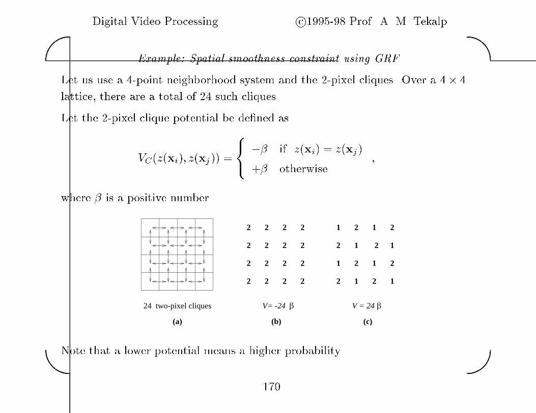
Digital Video Processing c�������� Prof� A� M� Tekalp��
��
Example� Spatial smoothness constraint using GRF
Let us use a �point neighborhood system and the ��pixel cliques� Over a
lattice� there are a total of � such cliques�
Let the ��pixel clique potential be dened as
VC�z�xi� z�xj ���
� �� if z�xi � z�xj
�� otherwise
�
where � is a positive number�
2 2 2 2
2222
2
2 2 2 2
222
2
2
1
1 1
1 1
1 1
12 2
2
2 2
2
β β
(a) (b) (c)
V = 24V= -2424 two-pixel cliques
Note that a lower potential means a higher probability�
���
Digital Video Processing c�������� Prof� A� M� Tekalp��
��
Equivalence of GRF and MRF
Hammersley�Cli�ord �H�C� Theorem� Let N be a neighborhood system�
Then z�x is an MRF with respect to N if and only if p�z is a Gibbsian with
respect to N �
� The H�C theorem provides us with a simple and practical way to specify MRFs
through the Gibbs potentials�
� In general� the MRF is specied in terms of local conditional pdfs� Note that�
there is no general method to obtain the joint pdf of an MRF from the local
conditional pdfs �Besag��
� The Gibbs distribution gives the joint pdf of z� which can be easily expressed
in terms of the clique potentials which express the local interaction between
pixels� They can be assigned arbitrarily����

Digital Video Processing c�������� Prof� A� M� Tekalp��
��
Obtaining Local Conditional pdfs from Gibbs Potentials
e�g�� used in the Gibbs sampler method for optimization
� The local conditional pdf is dened as�
p�z�xi j z�xj��xj �� xi �
p�z
p�z�xj�xj �� xi
�
p�zPz�xi���p�z� � xi � �
� After some algebra�
p�z�xi j z�xj��xj �� xi � Q��xie� �T
PCjxi�C
VC�z�x�jx�C��
where
Qxi
�
Xz�xi���
e� �T
PCjxi�C
VC�z�x�jx�C�
���

Digital Video Processing c�������� Prof� A� M� Tekalp��
��
OPTIMIZATION METHODS
� Many estimation�segmentation problems require the minimization of an energy
function E�d� We state the problem as
�E � mindE�d
where d is some N �dimensional parameter vector� The value of d that results in
the minimal E is denoted by�d � arg �mindE�d
� This minimization is exceedingly di�cult for image processing applications due
to both the dimensions of the vectors involved and the occurence of local minima
because E�d is usually nonconvex�
���
Digital Video Processing c�������� Prof� A� M� Tekalp��
��
Local vs� Global Minima
� Gradient descent su�ers from a serious problem� its solution is strongly
dependent on the starting point� If start in a �valley�� it will be stuck at the
bottom of that valley� We have no way of getting out of that local minimum to
reach the �global� minimum�
� Here we look at several optimization methods that are capable of nding the
global optimum�
A� Simulated annealing �stochastic relaxation
Metropolis algorithm�
Gibbs sampler �by Geman and Geman�
B� Iterative conditional mode �ICM �by Besag
C� Mean �eld annealing �MFA �by Bilbro et al�
��

Digital Video Processing c�������� Prof� A� M� Tekalp��
��
Simulated Annealing
� Simulated annealing� sometimes refered to as stochastic relaxation� belongs to
the class of Monte Carlo methods�
� It enables us to nd the global optimum of a nonconvex cost function of many
variables�
� Here we describe two implementations�
� the original formulation of Metropolis and
� the Gibbs sampler proposed by Geman and Geman�
� The computational load of simulated annealing is usually signicant especially
when the number of elements in the unknown vector d and the number of values
in the set � are large�
���
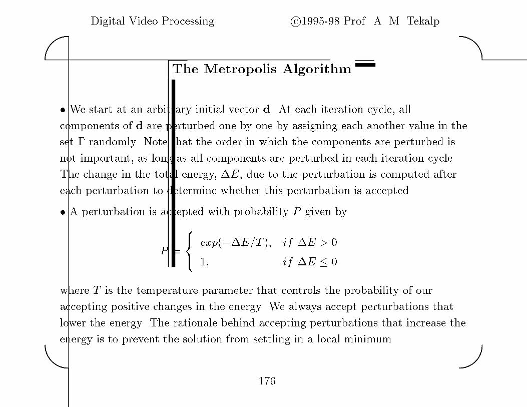
Digital Video Processing c�������� Prof� A� M� Tekalp��
��
The Metropolis Algorithm
� We start at an arbitrary initial vector d� At each iteration cycle� all
components of d are perturbed one by one by assigning each another value in the
set � randomly� Note that the order in which the components are perturbed is
not important� as long as all components are perturbed in each iteration cycle�
The change in the total energy� �E� due to the perturbation is computed after
each perturbation to determine whether this perturbation is accepted�
� A perturbation is accepted with probability P given by
P ���
� exp���E�T � if �E � �
�� if �E � �
where T is the temperature parameter that controls the probability of our
accepting positive changes in the energy� We always accept perturbations that
lower the energy� The rationale behind accepting perturbations that increase the
energy is to prevent the solution from settling in a local minimum�
���

Digital Video Processing c�������� Prof� A� M� Tekalp��
��
� If T is relatively big� the probability of accepting a positive
energy change is higher than when T is small� given the same �E� In the next
iteration cycle� the temperature is lowered� and the
components are revisited� The process continues until the
temperature has been lowered to near zero�
� A temperature �schedule�� expressing temperature as a
function of the iteration number� is therefore an important
component in the stochastic relaxation process� Geman and Geman proposed the
following schedule
T �
�
ln�k � ��
where � is a constant and k is the iteration cycle� This schedule is viewed as over
conservative but guarantees a global minimum solution� Schedules that lower the
temperature at a faster rate have been shown to work�
���

Digital Video Processing c�������� Prof� A� M� Tekalp��
��
The Algorithm
�� Choose an initial value for d � d���� Set i � � and j � ��
�� Perturb the jth component of d�i� to generate the vector d�i����
�� Compute �E � E�d�i���� E�d�i��
� Compute P fromP �
��� exp���E�T � if �E � �
�� if �E � �
�� If P �� then draw a random number that is uniformly distributed between �
and �� If the number drawn is less than P accept the perturbation�
�� Set j � j � �� If j � N � go to �� �N is the number of components of d�
�� Set i � i� � and j � �� Reduce T according to a temperature schedule� If
T � Tmin� go to �� Otherwise terminate����
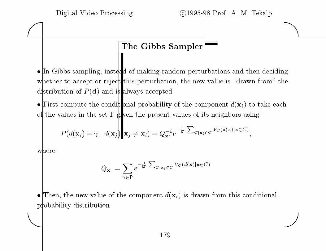
Digital Video Processing c�������� Prof� A� M� Tekalp��
��
The Gibbs Sampler
� In Gibbs sampling� instead of making random perturbations and then deciding
whether to accept or reject this perturbation� the new value is �drawn from� the
distribution of P �d and is always accepted�
� First compute the conditional probability of the component d�xi to take each
of the values in the set � given the present values of its neighbors using
P �d�xi � j d�xj�xj �� xi � Q��xie� �T
PCjxi�C
VC�d�x�jx�C��
where
Qxi
�X
���e� �T
PCjxi�C
VC�d�x�jx�C�
� Then� the new value of the component d�xi is drawn from this conditional
probability distribution�
���
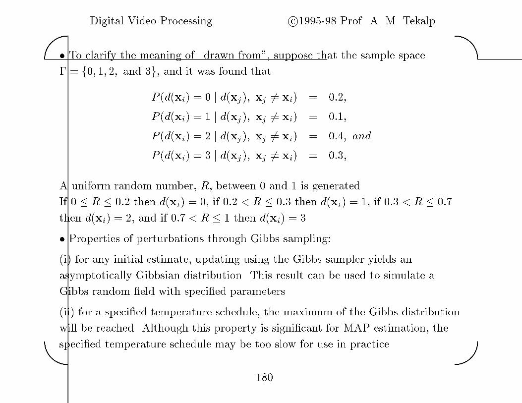
Digital Video Processing c�������� Prof� A� M� Tekalp��
��
� To clarify the meaning of �drawn from�� suppose that the sample space
� � f�� �� �� and �g� and it was found that
P �d�xi � � j d�xj� xj �� xi � ����
P �d�xi � � j d�xj� xj �� xi � ����
P �d�xi � � j d�xj� xj �� xi � �� � and
P �d�xi � � j d�xj� xj �� xi � ����
A uniform random number� R� between � and � is generated�
If � � R � ��� then d�xi � �� if ��� R � ��� then d�xi � �� if ��� R � ���
then d�xi � �� and if ��� R � � then d�xi � ��
� Properties of perturbations through Gibbs sampling�
�i for any initial estimate� updating using the Gibbs sampler yields an
asymptotically Gibbsian distribution� This result can be used to simulate a
Gibbs random eld with specied parameters�
�ii for a specied temperature schedule� the maximum of the Gibbs distribution
will be reached� Although this property is signicant for MAP estimation� the
specied temperature schedule may be too slow for use in practice�
���

Digital Video Processing c�������� Prof� A� M� Tekalp��
��
Iterated Conditional Modes �ICM�
� ICM� also referred to as the greedy algorithm� is motivated by a need to reduce
the computational load produced by stochastic relaxation or Gibbs sampling�
� Here� the sites are again visited one�by�one in some cyclic fashion� except there
is no temperature change involved� The temperature T is set to zero� T � � for
all iterations� Therefore� ICM is also refered to as the �instant freezing� case of
simulated annealing�
� Refering to the equation of acceptance probability in SA� ICM only allows
perturbations that provide negative �E� since T � � e�ectively gives a zero
probability for accepting positive energy changes�
� Notice that due to this� solutions from ICM is likely to get trapped in local
minima� and there is no guarantee that a global minimum can be reached�
���

Digital Video Processing c�������� Prof� A� M� Tekalp��
��
� It can be shown that ICM converges to the solution that maximizes the local
conditional probabilities
P �d�xi � j d�xj�xj �� xi � Q��xie� �T
PCjxi�C
VC�d�x�jx�C��
where
Qxi
�X
���e� �T
PCjxi�C
VC�d�x�jx�C�
at each site� Thus� ICM is usually implemented as in Gibbs sampling but by
choosing the value at each site that gives the maximum local conditional
probability�
� ICM provides a much faster convergence than SA� Also� when the initial
solution is a resonable estimate from other means rather than completely
random� ICM reaches an acceptable solution in relatively few iterations� ICM
produces good results for several applications that include image restoration �see
Besag� and image segmentation �see Pappas��
���
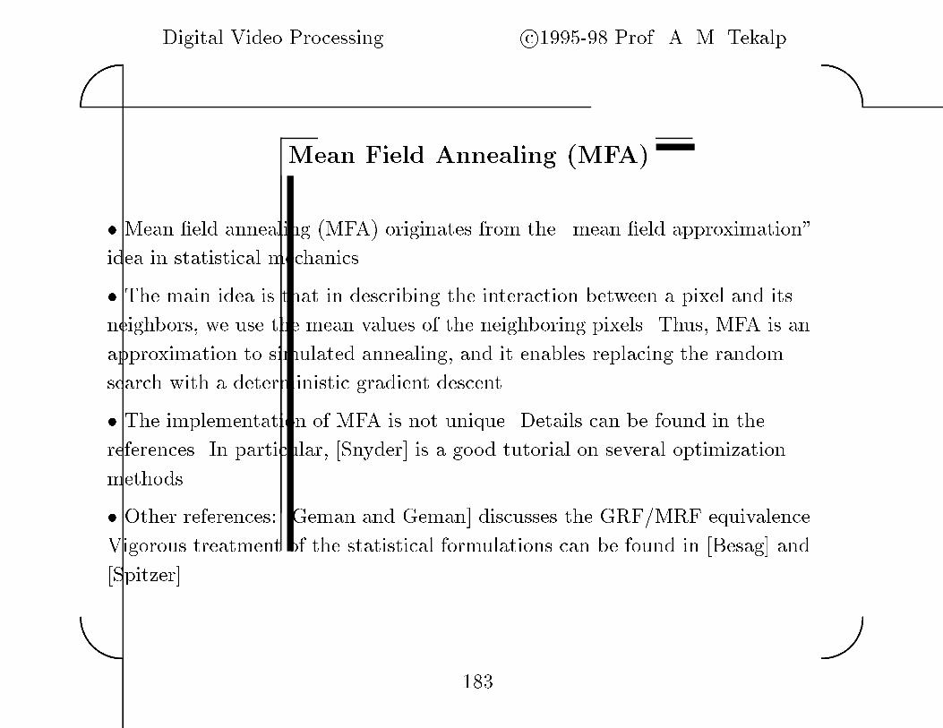
Digital Video Processing c�������� Prof� A� M� Tekalp��
��
Mean Field Annealing �MFA�
� Mean eld annealing �MFA originates from the �mean eld approximation�
idea in statistical mechanics�
� The main idea is that in describing the interaction between a pixel and its
neighbors� we use the mean values of the neighboring pixels� Thus� MFA is an
approximation to simulated annealing� and it enables replacing the random
search with a deterministic gradient descent�
� The implementation of MFA is not unique� Details can be found in the
references� In particular� �Snyder� is a good tutorial on several optimization
methods�
� Other references� �Geman and Geman� discusses the GRF�MRF equivalence�
Vigorous treatment of the statistical formulations can be found in �Besag� and
�Spitzer��
���
Digital Video Processing c�������� Prof� A� M� Tekalp��
��
BAYESIAN MOTION ESTIMATION
Letsk � fsk�xg� x � �� denote the kth frame of video�
d�x � �d��x d��x�T denote the displacement vector at site x� and
d� � fd��xg and d� � fd��xg for x � �� denote the lexicographic ordering of
the x� and x� components of the displacement eld from frame k � � to k�
respectively
i�e�� sk�x � sk���x� d�x�
Then� the problem of motion estimation can be formulated as�
given sk and sk��� nd an estimate of d� and d��
The maximum a posteriori probability �MAP estimates of d� and d� are given
by�
��d�� �d� � arg maxd��d� p�d��d�jsk� sk��
��

Digital Video Processing c�������� Prof� A� M� Tekalp��
��
From Bayes formula
p�d��d�jsk� sk�� �p�skjd��d�� sk��p�d��d�jsk��
p�skjsk��
Since the denominator is not a function of d� and d��
��d�� �d� � arg maxd��d� p�skjd��d�� sk��p�d��d�jsk��
or
��d�� �d� � arg maxd��d� p�sk��jd��d�� skp�d��d�jsk
� The term p�skjd��d�� sk�� is the conditional pdf� or the �consistency
�likelihood measure�� that measures how well the estimates of d�� d� explain
the observations sk given sk���
� The term p�d��d�jsk�� is the a priori probability density that is modeled by a
GRF� by specifying the clique potential functions according to the desired local
properties of ��d�� �d��
���
Digital Video Processing c�������� Prof� A� M� Tekalp��
��
Discontinuity Models
� Let us introduce two auxilary elds� the occlusion eld o� and the line eld l to
model the occlusion�uncovered areas� and the optical ow boundaries
respectively� in order to improve the motion estimation results�
The occlusion �eld
o � o�x� x � ��
o�x ���
� � d�x is well dened
� x is an occlusion point
The line �eld
The a priori pdf p�d��d�jsk�� is usually chosen to favor a globally smooth
motion eld� To allow for the presence of discontinuities in the motion eld� we
make use of the line process�
���
Digital Video Processing c�������� Prof� A� M� Tekalp��
��
The line eld l�xi�xj models the horizontal and vertical discontinuities in the
motion eld �optical ow between the sites xi and xj as
l�xi�xj �����
���� if there is a discontinuity
between d�xiand d�xj
� otherwise�
� The line process� l conceptually occupies the dual lattice which has sites for
lines between every pair of pixel sites� The state of each line site can be either
ON �l � � or OFF �l � �� expressing the presence and absence of a
discontinuity� respectively�
� Nonnegative potentials are assigned to each rotation invariant line clique
conguration to penalize excessive use of the �ON� state�
���
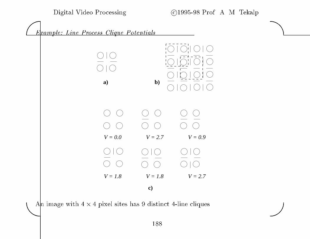
Digital Video Processing c�������� Prof� A� M� Tekalp��
��
Example� Line Process Clique Potentials
c)
a) b)
V = 1.8 V = 1.8 V = 2.7
V = 0.0 V = 2.7 V = 0.9
An image with pixel sites has � distinct �line cliques�
���
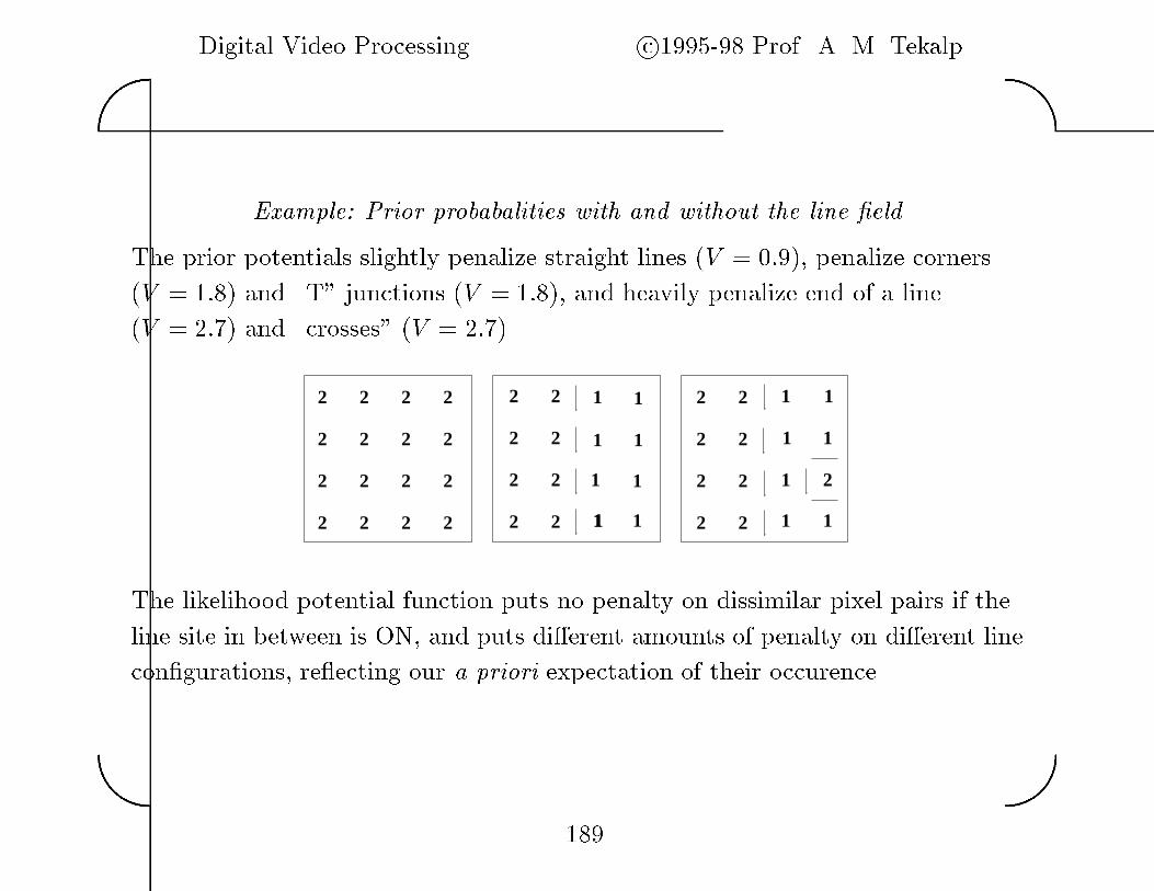
Digital Video Processing c�������� Prof� A� M� Tekalp��
��
Example� Prior probabalities with and without the line �eld
The prior potentials slightly penalize straight lines �V � ���� penalize corners
�V � ��� and �T� junctions �V � ���� and heavily penalize end of a line
�V � ��� and �crosses� �V � ����
2 2 2 2
2222
2
2 2 2 2
222
2 2
22
2
2 2
2
2 2
22
2
2 2
2
1
1 1
1
11 1
1
1 1 1
1 1
1
1 1
2
The likelihood potential function puts no penalty on dissimilar pixel pairs if the
line site in between is ON� and puts di�erent amounts of penalty on di�erent line
congurations� re ecting our a priori expectation of their occurence�
���

Digital Video Processing c�������� Prof� A� M� Tekalp��
��
� With the introduction of the auxiliary elds� the MAP estimate of fd��d��o� lg
is given by�f�d�� �d�� �o��lg � arg maxd��d��o�l p�d��d��o� ljsk� sk��
Using the Bayes rule� and the symmetry of the expression
f�d�� �d�� �o��lg � arg maxd��d��o�l p�sk��jd��d��o� l� skp�d��d��o� ljsk
Next� we discuss the likelihood �consistency and the a priori probability models�
���
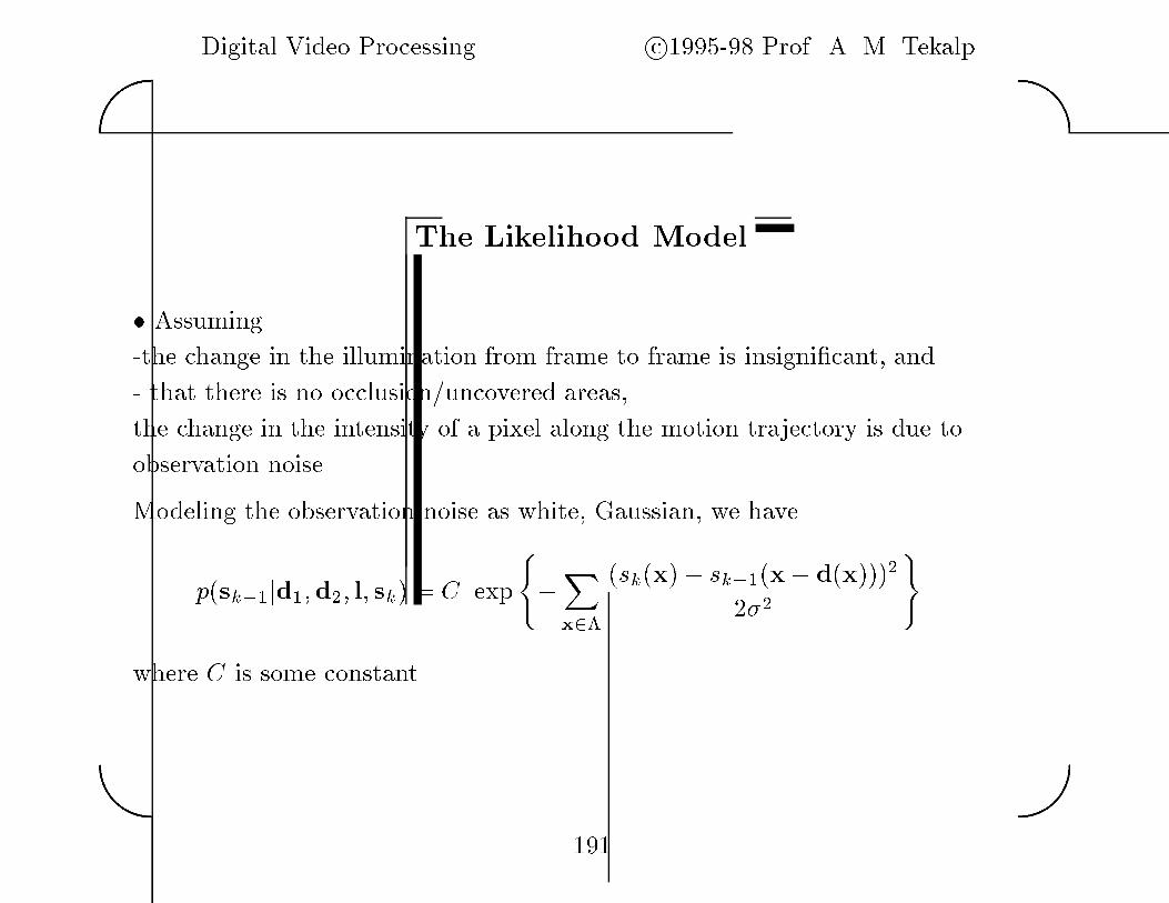
Digital Video Processing c�������� Prof� A� M� Tekalp��
��
The Likelihood Model
� Assuming
�the change in the illumination from frame to frame is insignicant� and
� that there is no occlusion�uncovered areas�
the change in the intensity of a pixel along the motion trajectory is due to
observation noise�
Modeling the observation noise as white� Gaussian� we have
p�sk��jd��d�� l� sk � C exp�
�X
x��sk�x� sk���x� d�x�
���
�
where C is some constant�
���
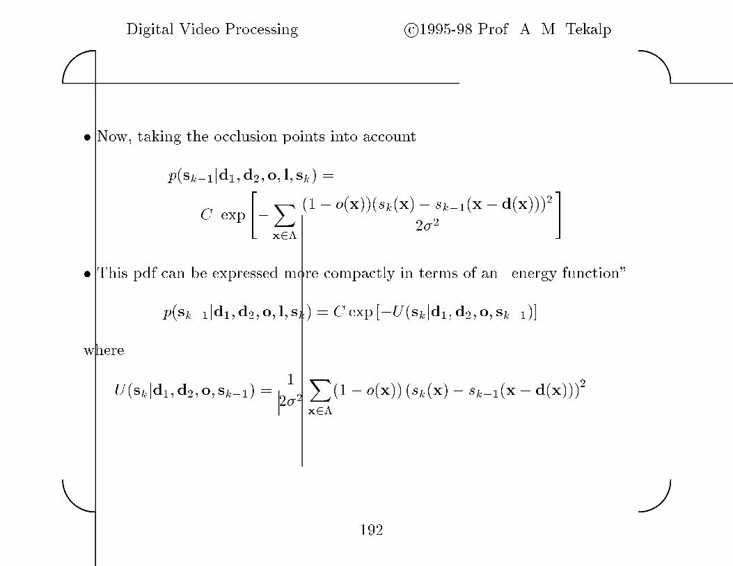
Digital Video Processing c�������� Prof� A� M� Tekalp��
��
� Now� taking the occlusion points into account
p�sk��jd��d��o� l� sk �
C exp�
�X
x���� o�x�sk�x� sk���x� d�x�
���
�
� This pdf can be expressed more compactly in terms of an �energy function�
p�sk��jd��d��o� l� sk � C exp ��U�skjd��d��o� sk���
whereU�skjd��d��o� sk�� �
����X
x���� o�x �sk�x� sk���x� d�x�
���
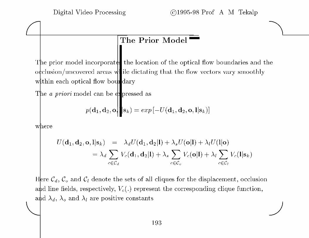
Digital Video Processing c�������� Prof� A� M� Tekalp��
��
The Prior Model
The prior model incorporates the location of the optical ow boundaries and the
occlusion�uncovered areas while dictating that the ow vectors vary smoothly
within each optical ow boundary�
The a priori model can be expressed as
p�d��d��o� ljsk � exp ��U�d��d��o� ljsk�
whereU�d��d��o� ljsk � �dU�d��d�jl � �sU�ojl � �lU�ljo
� �dX
c�CdVc�d��d�jl � �sX
c�CoVc�ojl � �lX
c�ClVc�ljsk
Here Cd� Co and Cl denote the sets of all cliques for the displacement� occlusion
and line elds� respectively� Vc�� represent the corresponding clique function�
and �d� �o and �l are positive constants����
Digital Video Processing c�������� Prof� A� M� Tekalp��
��
ESTIMATION ALGORITHMS
The minimization of the overall potential is an exceedingly di�cult problem�
� there are several hundreds of thousands of unknowns for a reasonable size
image� and
� the criterion function is nonconvex�
For example� for a ��� ��� image� there are ������ motion vectors ��������
components� ������ occlusion labels� and ������� line eld labels for a total of
������� unknowns�
An additional complication is that the motion vector components are
continuous�valued� and the occlusion and line eld labels are discrete�valued�
��

Digital Video Processing c�������� Prof� A� M� Tekalp��
��
Three�step iteration of Dubois and Konrad�
�� Given the best estimates of the auxilary eld �o and �l� update the motion
eld dk by minimizing
min
d��d�
Ug�gk�d��d�� �o�gk�� � �dUd�d��d���l�gk
This minimization can be done by Gauss�Newton optimization�
�� Given the best estimates of �d�� �d� and �l� update o by minimizing
mino
Ug�gk� �d�� �d��o�gk�� � �oUo�o��l�gk
An exhaustive search or the ICM method can be employed to solve this step�
�� Finally� given the best estimates of �d�� �d� and �o� update l by minimizing
minl
�dUd��d�� �d�� l�gk�� � �oUo��o� l�gk � �lUl�l�gk
Once all three elds are updated� the process is repeated until a suitable
criterion of convergence is satised� This procedure has been reported to
give good results�
���
Digital Video Processing c�������� Prof� A� M� Tekalp��
��
LECTURE �
MOTION SEGMENTATION
�� Basics of Segmentation
� Thresholding � Clustering � MAP Segmentation
�� Foreground�Background Separation
� Dominant Motion vs� Parametric Clustering Methods
� Direct Methods vs� Optical Flow Segmentation
�� Simultaneous MAP Motion Estimation and Segmentation
�� Integration of Color and Motion Segmentation
���

Digital Video Processing c�������� Prof� A� M� Tekalp��
��
WHY OBJECT�MOTION SEGMENTATION�
� Help improve optical �ow estimation with multiple motion
� Help improve �D motion and structure estimation
� Object�based video coding
� Object�based editing synthetic trans�guration�
���

Digital Video Processing c�������� Prof� A� M� Tekalp��
��
Image vs� Optical Flow Segmentation
� Segmentation is based on a feature vector��
e�g�� image segmentation usually refers to segmentation based upon
the grayscale or color� of pixels�
� Application of standard image segmentation methods directly to optical �ow
segmentation i�e�� using the velocity vector as feature� may not be useful�
since �D motion usually generates spatially varying optical �ow �elds�
e�g�� within a purely rotating object� there is no �ow at the center of
rotation and the magnitude of the �ow vectors increase as the distance
of the points from the center of rotation increase�
� Thus� optical �ow segmentation needs to be based on some parametric
description of the motion �eld�
���
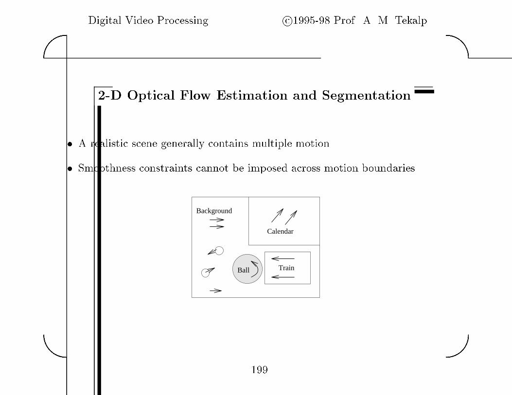
Digital Video Processing c�������� Prof� A� M� Tekalp��
��
��D Optical Flow Estimation and Segmentation
� A realistic scene generally contains multiple motion�
� Smoothness constraints cannot be imposed across motion boundaries�
Background
Calendar
TrainBall
���

Digital Video Processing c�������� Prof� A� M� Tekalp��
��
��D Motion�Structure Estimation and Segmentation
� Assume that the object surface is composed of planar patches�
aX� � bX� � cX� � �
� The �D rigid motion of the object is modeled as����X
��
X�
�X
��
���� � R
����X�
X�X�
�����T
� Then� ����X
��
X�
�X
��
���� �
����a� a� a�
a� a� a�
a� a� a�
����
���X�
X�X�
����
where
A � R � T � a b c �
���

Digital Video Processing c�������� Prof� A� M� Tekalp��
��
Scene Segmentation
� Orthographic projection of the object coordinates into the image plane yields
x�� � a�x� � a�x� � a�
x�� � a�x� � a�x� � a�
� Perspective projection of the object coordinates into the image plane yields
x�� �
a�x� � a�x� � a�
a�x� � a�x� � �
x�� �
a�x� � a�x� � a�
a�x� � a�x� � �
� Assuming the scene is represented by a �D mesh wireframe� model with
planar patches� di�erent parametric models are needed for
� Di�erent moving objects� which have di�erent set of �D rigid
motion parameters�
� Di�erent planar patches� which have di�erent normal vectors�
���
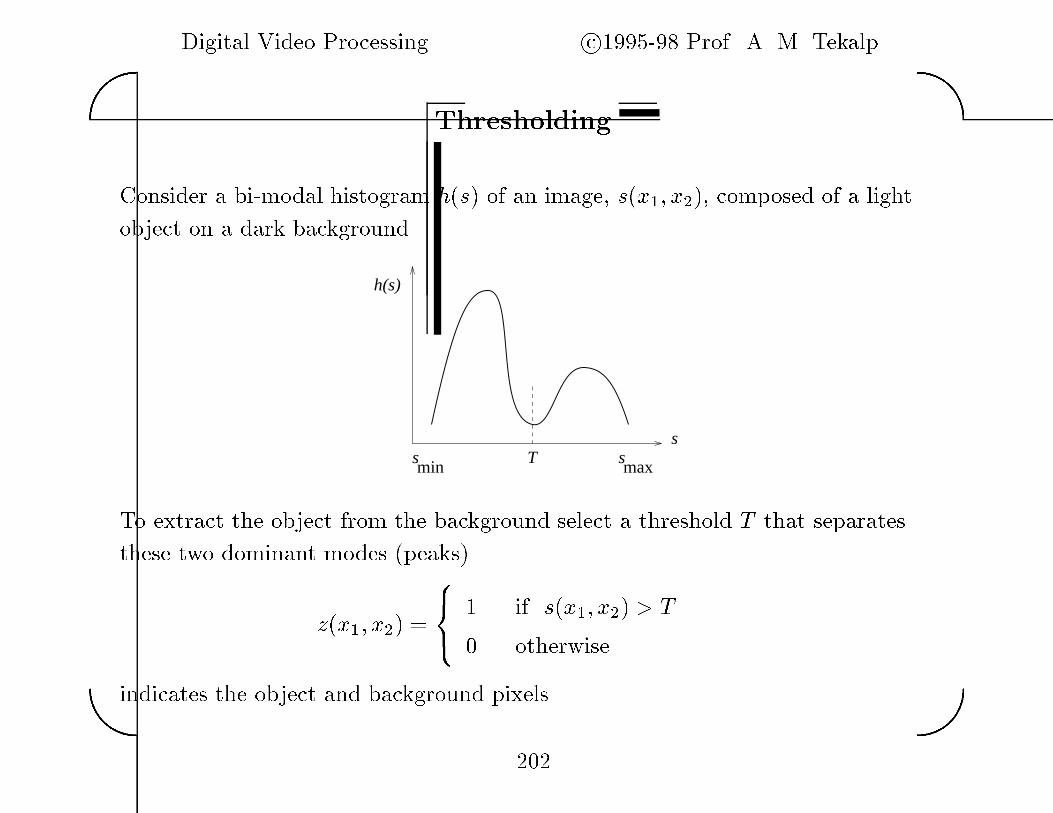
Digital Video Processing c�������� Prof� A� M� Tekalp��
��
Thresholding
Consider a bi�modal histogram h s� of an image� s x�� x��� composed of a light
object on a dark background�
h(s)
ssmaxmins T
To extract the object from the background select a threshold T that separates
these two dominant modes peaks�
z x�� x�� ���
� if s x�� x�� � T
� otherwise�
indicates the object and background pixels�
���
Digital Video Processing c�������� Prof� A� M� Tekalp��
��
� Multilevel Thresholding
If the histogram has M signi�cant modes peaks�� where M � �� then we need
M � � thresholds to separate the image into M segments� Of course� reliable
determination of the thresholds becomes more di�cult as the number of modes
increases�
� Global�Local�Dynamic Thresholding
In general� the threshold T is a function of
T � T x�� x�� s x�� x��� p x�� x���
where x�� x�� are the coordinates of a point� s x�� x�� is the intensity of the
point� and p x�� x�� is some local property of the point� such as the average
intensity of a local neighborhood�
If T depends only on s x�� x��� it is called a global threshold�
If T depends on both s x�� x�� and p x�� x��� it is a local threshold�
If� in addition� it depends on x�� x��� it is called a dynamic threshold�
� Methods for determining the threshold s� are discussed in Gonzalez and Wintz�
��

Digital Video Processing c�������� Prof� A� M� Tekalp��
��
Clustering via the K�Means Algorithm
Suppose we wish to segment an image into K regions based on the gray�values of
the pixels� Let x � x�� x�� denote the coordinates of a pixel� and s x� denote its
grey level�
µ µ
s
21
K = 2, M=1
� The K�means method of clustering minimizes the performance index
J �
KXk�
��� X
x���i�
k
jjs x�� ��i ��
k jj��
��
��

Digital Video Processing c�������� Prof� A� M� Tekalp��
��
The K�means Algorithm�
�� Choose K initial cluster centers� ����
� � ����
� � � � � � ����
K �
�� At the i�th iteration distribute the pixels� x� among the K clusters using the
relation
x � ��i�
j if jjs x�� ��i�
j jj � jjs x�� ��i�
k jj
for all k � �� �� � � � �K� k �� j� where ��i�
k denotes the set of samples whose cluster
center is ��i�
k �
� Compute the new cluster centers ��i ��
k � k � �� �� � � � �K as the sample mean of
all samples in ��i�
k
��i ��
k �
�Nk
Xx���i�k
s x�� k � �� �� � � � �K
where Nk is the number of samples in ��i�
k �
� If ��i ��
k � ��i�
k for all k � �� �� � � � �K� the algorithm has converged� and the
procedure is terminated� Otherwise� go to step ��
���
Digital Video Processing c�������� Prof� A� M� Tekalp��
��
MAP Segmentation
Clustering with Spatial Smoothness Constraints
Let z x� denote the segmentation label at the pixel x� i�e�� � � z x� � K� and
s x� denote the grey level of the pixel�
De�ne z and s to denote the lexicographic ordering of the segmentation label
�eld and the grey level �eld� respectively�
� The maximum a posteriori probability MAP� estimate of the segmentation
label �eld maximizes the a posteriori probability of the segmentation labels given
the pixel gray levels
p zjs� � p s j z�p z�
where p s j z� is the conditional probability density of the image grey levels given
the pixel labels and p z� is the prior density of the segmentation labels�
���

Digital Video Processing c�������� Prof� A� M� Tekalp��
��
The A Priori Probability Density
The prior pdf of the segmentation labels is modeled by an GRF
p z� �
�Q
X���exp
�X
C
VC z��
� z� ��
where Q is the partition function normalizing constant� and the summation is
over all cliques C� We consider only one and two point cliques�
� The single pixel clique potentials are de�ned as
VC z x�� � �i if z x� � i and x � C� all i
They re�ect our a priori knowledge of the probabilities of di�erent region types�
The smaller �i the higher the likelihood of region i�
� The two�point clique potentials are de�ned as
VC z x��� z x��� ���
� if z x�� � z x�� and x�� x� � C�
if z x�� �� z x�� and x�� x� � C
where is a positive parameter so that two neighboring pixels are more likely to
belong to the same class than to di�erent classes� The larger the value of � the
stronger the smoothness constraint�
���

Digital Video Processing c�������� Prof� A� M� Tekalp��
��
The Conditional Probability Density
The conditional density for region k is modeled as a white Gaussian process�
with mean �k and variance ��
Thus� the a posteriori density has the form
p zjs� � exp
�X
x
����
s x�� �z�x� �
�X
C
VC z��
� Maximization of this a posteriori density function with respect to z can be
performed by simulated annealing�
� Observe that if we turn o� the spatial smoothness constraints� the result is
identical to the K�means algorithm�
���
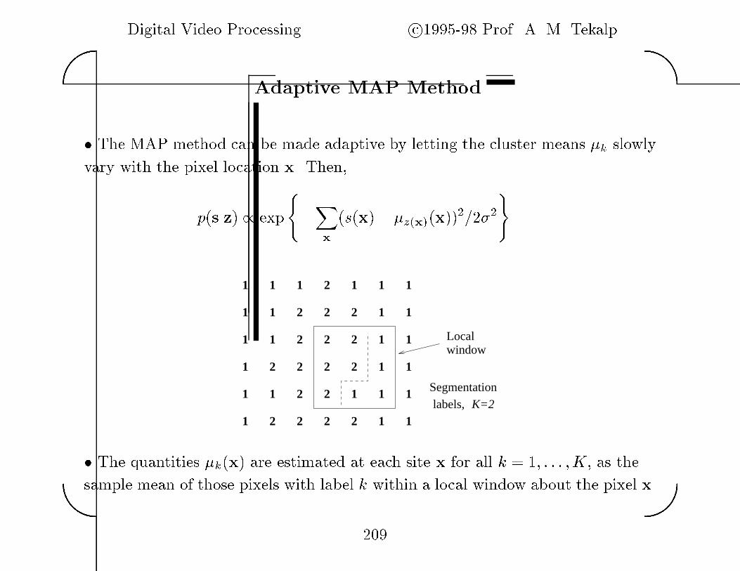
Digital Video Processing c�������� Prof� A� M� Tekalp��
��
Adaptive MAP Method
� The MAP method can be made adaptive by letting the cluster means �k slowly
vary with the pixel location x� Then�
p sjz� � exp
�X
x
s x�� �z�x� x�������
1
1 1
1
11
1
1
2
2
2 2
2
2
2
2
2
2
2
2
2
1 1 1
1 1
1
1
1
1 1
1
1
1
1
2 2 2 21 1 1
Localwindow
Segmentationlabels, K=2
� The quantities �k x� are estimated at each site x for all k � �� � � � �K� as the
sample mean of those pixels with label k within a local window about the pixel x�
���

Digital Video Processing c�������� Prof� A� M� Tekalp��
��
Computational Issues
� To reduce the computational load down to a reasonable level�
�� the space�varying mean estimates will be computed on a sparse grid� and then
interpolated�
�� the optimization will be performed via the ICM method�
� The algorithm starts with a window size equal to the image size and reduce the
size of the window by after each ICM optimization cycle�
� The ICM is equivalent to maximizing the local a posteriori pdf
p z xi�js x�� z xj�� all xj � Nxi�
� exp��
� ��� s x�� �z�x� x��� �
XCjx�C
VC z���
�
Ref� T� N� Pappas� �An Adaptive Clustering Algorithm for Image Segmentation�� IEEE Trans�
on Signal Proc�� vol� SP���� pp� ���� April ��
���
Digital Video Processing c�������� Prof� A� M� Tekalp��
��
Multi�Channel Segmentation
� Let y x� � v� x�� v� x�� s x��� Assign a single label z x� to each element of
y x� to maximize
p zjy� � p yjz�p z�
� Assuming v�� v�� and s are conditionally independent given z�
p v��v�� sjz� � p v�jz�p v�jz�p sjz�
which results in
p v��v�� sjz� � exp
�X
x
���� v� x�� �v�z�x� x����
���� v� x�� �v�z�x� x��� �
���� s x�� �sz�x� x����
� The prior pdf for s is a Gibbs distribution with a �pixel neighborhood system
and ��pixel cliques�
���
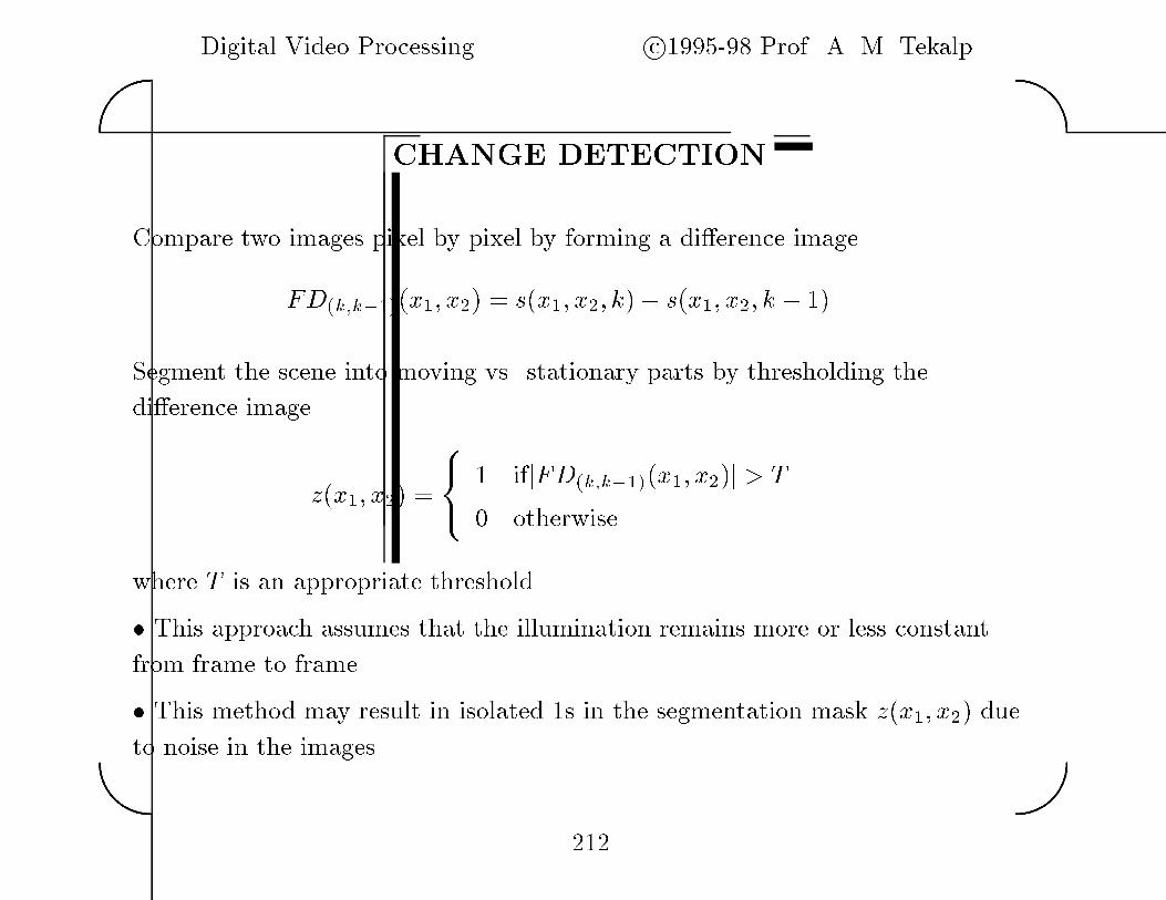
Digital Video Processing c�������� Prof� A� M� Tekalp��
��
CHANGE DETECTION
Compare two images pixel by pixel by forming a di�erence image
FD�k�k��� x�� x�� � s x�� x�� k�� s x�� x�� k � ��
Segment the scene into moving vs� stationary parts by thresholding the
di�erence imagez x�� x�� �
�� � ifjFD�k�k��� x�� x��j � T
� otherwise�
where T is an appropriate threshold�
� This approach assumes that the illumination remains more or less constant
from frame to frame�
� This method may result in isolated �s in the segmentation mask z x�� x�� due
to noise in the images�
���
Digital Video Processing c�������� Prof� A� M� Tekalp��
��
� Accumulative Di�erences
To eliminate sporadic ���s in the segmentation mask� we may consider adding
memory to the motion detection process by forming accumulative di�erence
images�
Let s x�� x�� k�� s x�� x�� k � ��� � � �� s x�� x�� k � n� be a sequence of images� and
let s x�� x�� k� be the reference frame�
An accumulative di�erence image is formed by comparing this reference image
with every subsequent image in the sequence� A counter for each pixel location
in the accumulative image is incremented every time the di�erence between the
reference image and the next image in the sequence at that pixel location is
bigger than the threshold�
��
Digital Video Processing c�������� Prof� A� M� Tekalp��
��
MOTION SEGMENTATION METHODS
� Dominant motion approach
Diehl� Hotter and Thoma� Bergen et al�� Burt et al�� Irani et al��
� Parameter clustering approach Adiv� Wang and Adelson�
� Simultaneous Bayesian estimation and segmentation Chang� et al��
� Region�based approach using color information Eren� et al��
��
Digital Video Processing c�������� Prof� A� M� Tekalp��
��
DOMINANT MOTION APPROACH
� Compute the dominant ��D translation in the entire region of analysis�
� Segment the region that corresponds to the computed motion by detecting
�stationary pixels� in the registered images�
� Employ a higher�order a�ne� perspective� model within this region for
improved motion estimation�
� Iterate steps �� until convergence�
� Proceed to the next dominant object by excluding the support of previously
computed dominant objects�
���

Digital Video Processing c�������� Prof� A� M� Tekalp��
��
A Direct Method
i� Parametric modeling of the ��D motion �eld
De�ne a transform with a set of parameters that maps pixels from frame k to
frame k��� Estimate the parameters of this transform in the image domain�
ii� Segmentation
Regions undergoing the same �D motion would have the same set of mapping
parameters� Thus� assign �ow vectors having the same mapping parameters into
the same class�
The process iterates between parameter estimation and segmentation until a
satisfactory result is obtained�
���

Digital Video Processing c�������� Prof� A� M� Tekalp��
��
Parametric Modeling of the ��D Motion Field
Let
gk x� � sk x� � nk x�
gk � x� � � � ��sk � x�� � � nk � x�
where � and describe global illumination changes� and nk x� denotes the noise�
� Assuming no occlusion e�ects�sk � x
�� � sk x�
� The transformation from the coordinate systems x to x�
is given by
x�
� h x���
where � is a parameter vector� The form of h x��� depends on�
�� The �D motion of the object�
�� The projection model from the �D space onto the camera plane�
� The model of the object surface planar� quadratice� etc��
���
Digital Video Processing c�������� Prof� A� M� Tekalp��
��
Examples of Coordinate Transforms
�� Planar surface� perspective projection�
Let x�
and x denote image plane coordinates under the perspective projection�
Assume that the surface of the moving object is planar� X� � aX� � bX� � c�
Then� the transformation is given by
x�
� �
a�x� � a�x� � a�
a�x� � a�x� � �
x�
� �
a�x� � a�x� � a�
a�x� � a�x� � �
where � � a�� � � � � a�� is the vector of mapping parameters�
�� Planar surface� orthographic projection�
In the case of parallel orthographic� projection� we have the a�ne transform
x�
� � c�x� � c�x� � c�
x�
� � c�x� � c�x� � c�
where � � c�� � � � � c�� is the vector of mapping parameters�
���
Digital Video Processing c�������� Prof� A� M� Tekalp��
��
� Quadratic surface� orthographic projection�
Let the surface be characterized by
X� � a��X�
� � a��X�X� � a��X�
� � a��X� � a��X� � a��
and the equations
x� � mX�� x� � mX�
x�
� � m�
X�
�� x�
� � m�
X�
�
describe the parallel projection�
Substituting these into the �D displacement model and grouping terms with the
same exponent� we arrive at the ���parameter quadratic transform
x�
� � a�x�
� � a�x�
� � a�x�x� � a�x� � a�x� � a�
x�
� � b�x�
� � b�x�
� � b�x�x� � b�x� � b�x� � b�
���

Digital Video Processing c�������� Prof� A� M� Tekalp��
��
Remarks�
� The quadratic transform is generally used in optical �ow segmentation and
object�oriented description� because it provides a good approximation to many
real life images�
� It is not always possible to completely determine the �D motion of the object
and the explicit surface structure using only the mapping parameters of the
transform h x���� But for image coding applications this does not pose a
serious problem� since the main interest is the prediction of the next frame from
the current frame�
� The mapping approach that is presented is not capable of handling occlusion
e�ects�
���

Digital Video Processing c�������� Prof� A� M� Tekalp��
��
Algorithms for Mapping Parameter Estimation
� We estimate the mapping parameters to minimize the error function
J ��� ��
�En
�sk � x� ���� sk � x���o
where �sk � x� ��� denotes the prediction of frame k � � from frame k�
� Linear algorithms exist to �nd the mapping parameters given spatio�temporal
intensity gradients� The contents of the images sk x� and sk � x� must be
su�ciently similar for estimation to be successful�
���

Digital Video Processing c�������� Prof� A� M� Tekalp��
��
Segmentation Based on Mapping Parameters
� Each object is characterized by a speci�c mapping vector �� Thus�
segmentation and motion estimation are treated as a combined problem�
� In the �rst step� the regions which have changed between sk x� and sk � x� are
determined change detection��
� All isolated connected�regions of the resulting segmentation are de�ned as
objects of hierarchy level one� For each of these objects� a parameter vector � of
a transform h x��� which relates the two images is estimated�
� Next� those regions of each object where the vector � is not valid are removed�
These regions are de�ned as objects of the second hierarchical level�
� For the objects of level two and the remaining parts of level one� the parameter
vectors � are estimated�
� Repeat the procedure� until the parameter vectors for each region are
consistent with the region�
���

Digital Video Processing c�������� Prof� A� M� Tekalp��
��
PARAMETER CLUSTERING APPROACH
� Dense motion estimation hierarchical� �step Lucas�Kanade�
� Start with randomly selected seed blocks initial regions�� estimate a�ne
parameters over each block�
� Merge regions with �similar� a�ne parameters to reduce the number of
classes�
� Update regions by classifying each pixel to one of the motion classes based
on similarity of the dense and the corresponding a�ne motion vectors�
where a �good� match can be found�
� Reestimate a�ne parameters over the updated regions� and iterate until
convergence
� Classify all �unassigned pixels� based on a DFD criterion�
��

Digital Video Processing c�������� Prof� A� M� Tekalp��
��
Optical Flow Segmentation
� Problem Statement�
Segment a scene into independently moving objects�
� Feature Selection�
� cannot use ��D motion vectors since in most cases motion vectors do vary
within a single �D moving object� e�g�� rotation�
� use the underlying �D motion parameters of the objects�
� An Application� Layered video representation
��
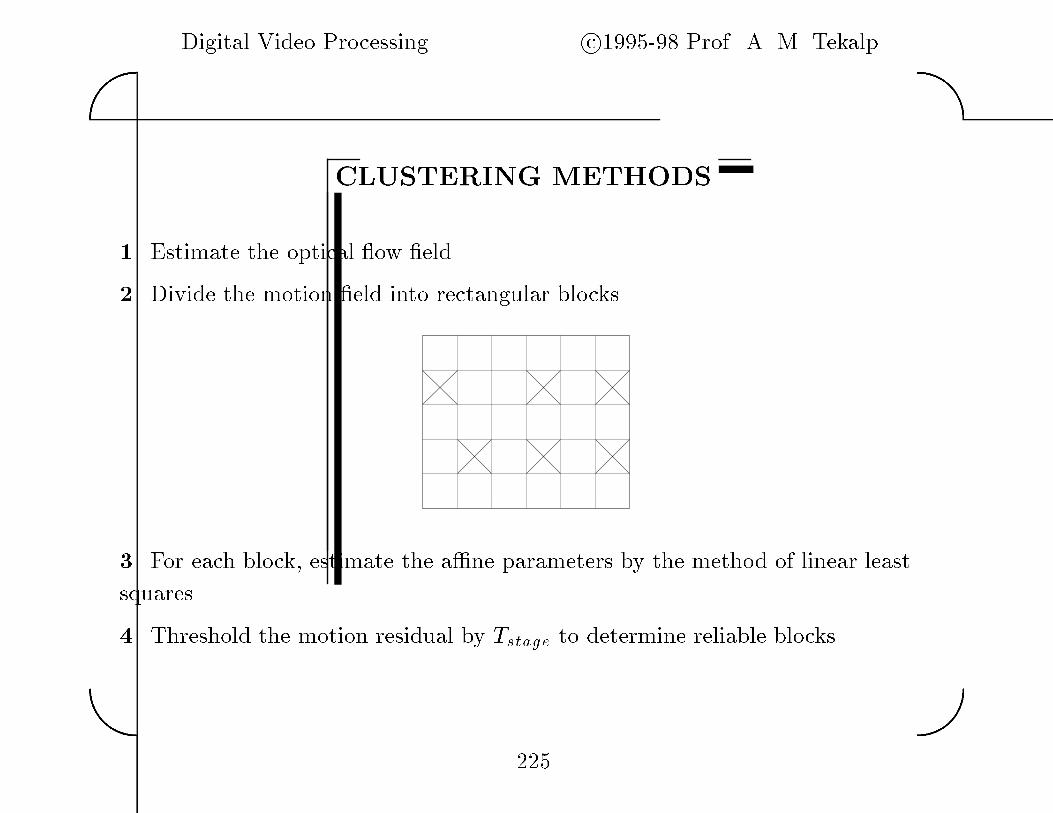
Digital Video Processing c�������� Prof� A� M� Tekalp��
��
CLUSTERING METHODS
�� Estimate the optical �ow �eld�
�� Divide the motion �eld into rectangular blocks�
�� For each block� estimate the a�ne parameters by the method of linear least
squares�
� Threshold the motion residual by Tstage to determine reliable blocks�
���
Digital Video Processing c�������� Prof� A� M� Tekalp��
��
� Apply the merge procedure to �nd the a�ne models to be used in pixel
assignment�
�� Find the pixels that fall into the computed cluster using the velocity checking
criterion�
�� Delete all the assigned pixels from the image so that they will not be used in
the next stage�
� Eliminate small regions from the map obtained in step ��
�� If all the pixels are assigned then stop� otherwise go to step �
���

Digital Video Processing c�������� Prof� A� M� Tekalp��
��
MAP SEGMENTATION
Maximize the a posteriori pdf of the label �eld
p zjv��v�� �p v��v�jz�p z�
p v��v��
given the optical �ow data� where p v��v�jz� is the conditional pdf of the optical
�ow data given the segmentation and p z� is the prior probability of the
segmentation�
�� The segmentation �eld is modeled by a spatio�temporal Markov random �eld
MRF� to impose continuity smoothness� of labels�
�� The conditional pdf models how well we can predict the measured estimated�
optical �ow �eld�
Ref� Murray and Buxton�
���
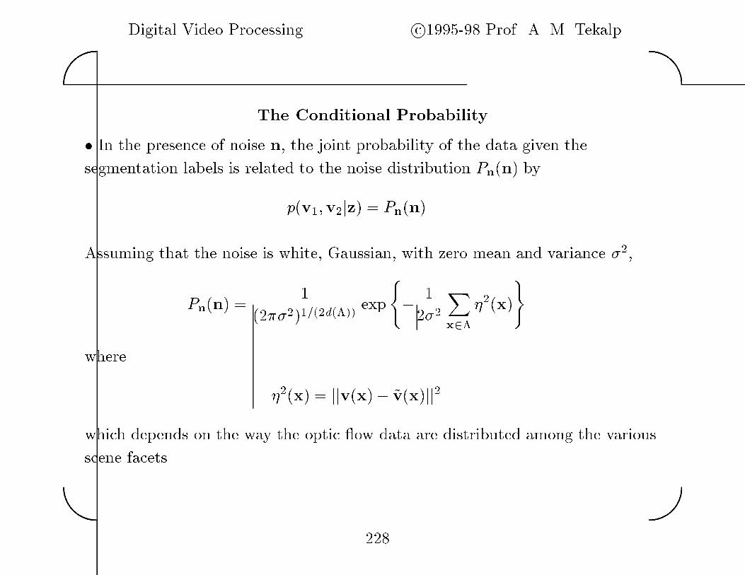
Digital Video Processing c�������� Prof� A� M� Tekalp��
��
The Conditional Probability
� In the presence of noise n� the joint probability of the data given the
segmentation labels is related to the noise distribution Pn
n� by
p v��v�jz� � Pn n�
Assuming that the noise is white� Gaussian� with zero mean and variance ��
Pn n� �
�
��������d����exp
�
���
Xx�� � x�
�
where
� x� � jjv x�� �v x�jj�
which depends on the way the optic �ow data are distributed among the various
scene facets�
���

Digital Video Processing c�������� Prof� A� M� Tekalp��
��
The Prior Probability
The prior probability of the interpretation is modeled by an MRF with respect
to some local neighborhood� Thus� it is given by a Gibbs distribution which
e�ectively introduces local constraints on the interpretation�
p z� �
�Q
X���exp f�U z�g � z� ��
where Q is the partition function
Q �X
���exp f�U ��g
and U �� is the sum of local potentials�
� Taking the logarithm of the MAP criterion� the maximization of the a
posteriori probability distribution becomes minimization of the cost function
���
Xx�� � x� � U z�
���
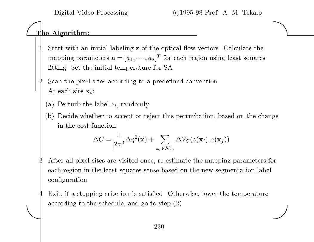
Digital Video Processing c�������� Prof� A� M� Tekalp��
��
The Algorithm�
�� Start with an initial labeling z of the optical �ow vectors� Calculate the
mapping parameters a � �a�� � � � � a��T for each region using least squares
�tting� Set the initial temperature for SA�
�� Scan the pixel sites according to a prede�ned convention�
At each site xi�
a� Perturb the label zi� randomly�
b� Decide whether to accept or reject this perturbation� based on the change
in the cost function
C �
��� � x� �
Xxj�Nxi VC z xi�� z xj��
� After all pixel sites are visited once� re�estimate the mapping parameters for
each region in the least squares sense based on the new segmentation label
con�guration�
� Exit� if a stopping criterion is satis�ed� Otherwise� lower the temperature
according to the schedule� and go to step ���
��
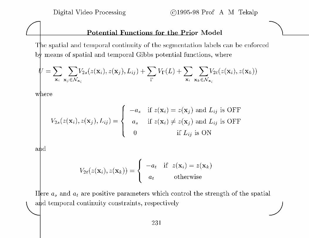
Digital Video Processing c�������� Prof� A� M� Tekalp��
��
Potential Functions for the Prior Model
The spatial and temporal continuity of the segmentation labels can be enforced
by means of spatial and temporal Gibbs potential functions� where
U �X
xi
Xxj�NxiV�s z xi�� z xj�� Lij� �X
�
V� L� �X
xi
Xxk�NxiV�t z xi�� z xk��
whereV�s z xi�� z xj�� Lij� �
������
�as if z xi� � z xj� and Lij is OFF
as if z xi� �� z xj� and Lij is OFF
� if Lij is ON
and
V�t z xi�� z xk�� ���
�at if z xi� � z xk�
at otherwise
Here as and at are positive parameters which control the strength of the spatial
and temporal continuity constraints� respectively�
��

Digital Video Processing c�������� Prof� A� M� Tekalp��
��
Simultaneous Motion Estimation and Segmentation
� The optical �ow segmentation methods are limited by the accuracy of the
available optical �ow estimates�
� Combine motion estimation and segmentation under a single MAP estimation
framework in a mutually bene�cial way�
� The posterior probability
p v��v�� zjgk�gk �� �p gk �jgk�v��v�� z�p v��v�jz�gk�p zjgk�
p gk �jgk�
� p gk �jgk�v��v�� z� is characterized by the DFD� modeled by a Gaussian
distribution�
� p zjgk� is modeled as Gibbsian for connected regions�
��

Digital Video Processing c�������� Prof� A� M� Tekalp��
��
� p v��v�jz�gk� relates the ��D motion estimates to the �D scene
p v��v�jz�gk� � p v��v�jz� �
�Qexp f�U v��v�jz�g
where
U v��v�jz� � �X
xi
Xxj�Nxijjv xi�� v xj�jj�� z xi�� z xj��
� �X
x
jjv x�� �v x�jj�
� Maximizing the a posteriori pdf is equivalent to minimizing the cost function�
C � U gk � j gk�v��v�� z� � U v��v� j z� � U z�
The minimization is performed in two steps� alternating between estimation of
optical �ow� estimation of the model parameters and update of segmentation
labels�
�
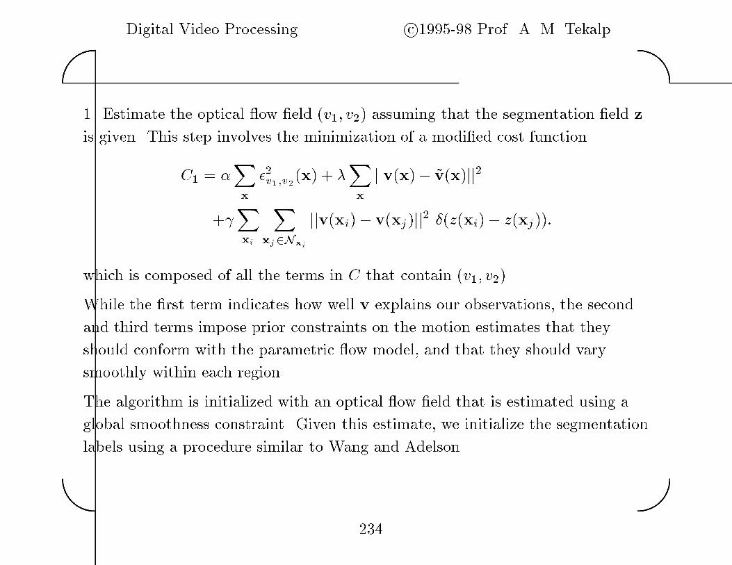
Digital Video Processing c�������� Prof� A� M� Tekalp��
��
�� Estimate the optical �ow �eld v�� v�� assuming that the segmentation �eld z
is given� This step involves the minimization of a modi�ed cost function
C� � �X
x
��v��v� x� � �X
x
jjv x�� �v x�jj�
��X
xi
Xxj�Nxijjv xi�� v xj�jj� � z xi�� z xj���
which is composed of all the terms in C that contain v�� v���
While the �rst term indicates how well v explains our observations� the second
and third terms impose prior constraints on the motion estimates that they
should conform with the parametric �ow model� and that they should vary
smoothly within each region�
The algorithm is initialized with an optical �ow �eld that is estimated using a
global smoothness constraint� Given this estimate� we initialize the segmentation
labels using a procedure similar to Wang and Adelson�
�
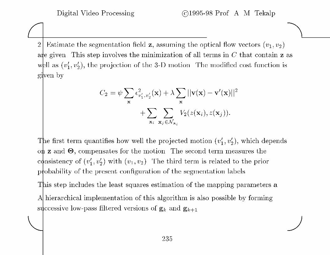
Digital Video Processing c�������� Prof� A� M� Tekalp��
��
�� Estimate the segmentation �eld z� assuming the optical �ow vectors v�� v��
are given� This step involves the minimization of all terms in C that contain z as
well as v��� v�
��� the projection of the �D motion� The modi�ed cost function is
given by
C� � �X
x
��v���v
�� x� � �X
x
jjv x�� v� x�jj�
�X
xi
Xxj�NxiV� z xi�� z xj���
The �rst term quanti�es how well the projected motion v��� v�
��� which depends
on z and �� compensates for the motion� The second term measures the
consistency of v��� v�
�� with v�� v��� The third term is related to the prior
probability of the present con�guration of the segmentation labels�
This step includes the least squares estimation of the mapping parameters a�
A hierarchical implementation of this algorithm is also possible by forming
successive low�pass �ltered versions of gk and gk ��
��

Digital Video Processing c�������� Prof� A� M� Tekalp��
��
FlowchartGo to next frame
2-D dense motion
(e.g., Lucas-Kanade)
Multi-stageparametric motion
segmentation(ext. of Wang-Adelson)
estimation
Input video
Update motion field given segmentation
Update segmentation given
motion field
(Chang, Tekalp, Sezan)
(Chang, Tekalp, Sezan)
Updates are based on the MAP criterion using Gibbsian priors�
��
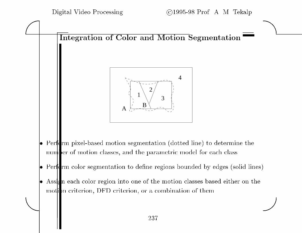
Digital Video Processing c�������� Prof� A� M� Tekalp��
��
Integration of Color and Motion Segmentation
12
3
4
A B
� Perform pixel�based motion segmentation dotted line� to determine the
number of motion classes� and the parametric model for each class�
� Perform color segmentation to de�ne regions bounded by edges solid lines��
� Assign each color region into one of the motion classes based either on the
motion criterion� DFD criterion� or a combination of them�
��
Related Documents