Chapter 2 2.1 Classify each of the following signals as finite or infinite. For the finite signals, find the smallest integer N such that x(k) = 0 for |k| >N . (a) x(k)= μ(k + 5) - μ(k - 5) (b) x(k) = sin(.2πk)μ(k) (c) x(k) = min(k 2 - 9, 0)μ(k) (d) x(k)= μ(k)μ(-k)/(1 + k 2 ) (e) x(k) = tan( √ 2πk)[μ(k) - μ(k - 100)] (f) x(k)= δ(k) + cos(πk) - (-1) k (g) x(k)= k -k sin(.5πk) Solution (a) finite, N =5 (b) infinite (c) finite, N =2 (d) finite, N =1 (e) finite, N = 99 (f) finite, N =0 (g) infinite 2.2 Classify each of the following signals as causal or noncausal. (a) x(k) = max{k, 0} (b) x(k) = sin(.2πk)μ(-k) (c) x(k)=1 - exp(-k) (d) x(k) = mod(k, 10) (e) x(k) = tan( √ 2πk)[μ(k)+ μ(k - 100)] (f) x(k) = cos(πk)+(-1) k (g) x(k) = sin(.5πk)/(1 + k 2 ) Solution (a) causal 51 c 2017 Cengage Learning. May not be scanned, copied or duplicated, or posted to a publicly accessible website, in whole or in part. Digital Signal Processing using MATLAB 3rd Edition Schilling Solutions Manual Full Download: http://testbanklive.com/download/digital-signal-processing-using-matlab-3rd-edition-schilling-solutions-manual/ Full download all chapters instantly please go to Solutions Manual, Test Bank site: testbanklive.com

Welcome message from author
This document is posted to help you gain knowledge. Please leave a comment to let me know what you think about it! Share it to your friends and learn new things together.
Transcript

Chapter 2
2.1 Classify each of the following signals as finite or infinite. For the finite signals, find thesmallest integer N such that x(k) = 0 for |k| > N .
(a) x(k) = µ(k + 5) − µ(k − 5)
(b) x(k) = sin(.2πk)µ(k)
(c) x(k) = min(k2 − 9, 0)µ(k)
(d) x(k) = µ(k)µ(−k)/(1 + k2)
(e) x(k) = tan(√
2πk)[µ(k)− µ(k − 100)]
(f) x(k) = δ(k) + cos(πk) − (−1)k
(g) x(k) = k−k sin(.5πk)
Solution
(a) finite, N = 5
(b) infinite
(c) finite, N = 2
(d) finite, N = 1
(e) finite, N = 99
(f) finite, N = 0
(g) infinite
2.2 Classify each of the following signals as causal or noncausal.
(a) x(k) = max{k, 0}(b) x(k) = sin(.2πk)µ(−k)
(c) x(k) = 1− exp(−k)
(d) x(k) = mod(k, 10)
(e) x(k) = tan(√
2πk)[µ(k) + µ(k − 100)]
(f) x(k) = cos(πk) + (−1)k
(g) x(k) = sin(.5πk)/(1 + k2)
Solution
(a) causal
51c© 2017 Cengage Learning. May not be scanned, copied or duplicated, or posted to a publicly accessible
website, in whole or in part.
Digital Signal Processing using MATLAB 3rd Edition Schilling Solutions ManualFull Download: http://testbanklive.com/download/digital-signal-processing-using-matlab-3rd-edition-schilling-solutions-manual/
Full download all chapters instantly please go to Solutions Manual, Test Bank site: testbanklive.com

(b) noncausal
(c) noncausal
(d) noncausal
(e) causal
(e) causal
(f) noncausal
2.3 Classify each of the following signals as periodic or aperiodic. For the periodic signals, findthe period, M .
(a) x(k) = cos(.02πk)
(b) x(k) = sin(.1k) cos(.2k)
(c) x(k) = cos(√
3k)
(d) x(k) = exp(jπ/8)
(e) x(k) = mod(k, 10)
(f) x(k) = sin2(.1πk)µ(k)
(g) x(k) = j2k
Solution
(a) periodic, M = 100
(b) nonperiodic, (τ = 20π)
(c) nonperiodic, (τ = 2π/√
3)
(d) periodic, M = 16
(e) periodic, M = 10
(f) nonperodic, (causal)
(g) periodic, M = 2
2.4 Classify each of the following signals as bounded or unbounded.
(a) x(k) = k cos(.1πk)/(1 + k2)
(b) x(k) = sin(.1k) cos(.2k)δ(k− 3)
(c) x(k) = cos(πk2)
(d) x(k) = tan(.1πk)[µ(k)− µ(k − 10]
(e) x(k) = k2/(1 + k2)
(f) x(k) = k exp(−k)µ(k)
52c© 2017 Cengage Learning. May not be scanned, copied or duplicated, or posted to a publicly accessible
website, in whole or in part.
Solution
(a) bounded
(b) bounded
(c) bounded
(d) unbounded
(e) bounded
(f) bounded
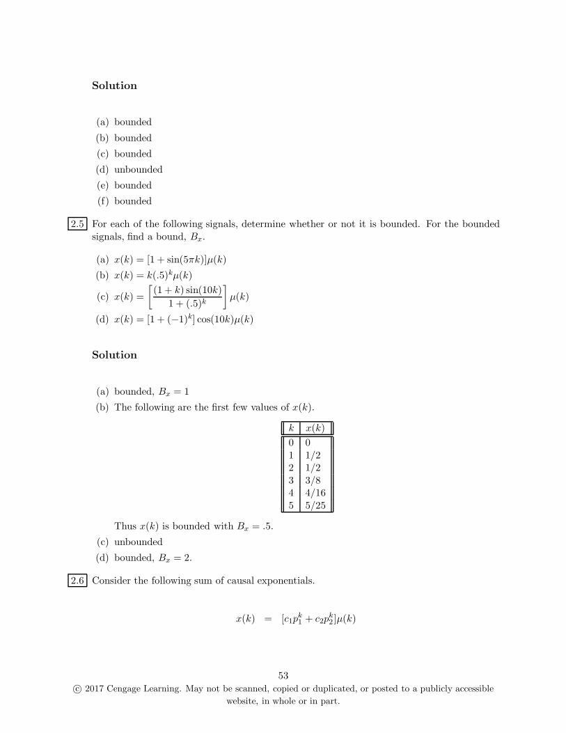
2.5 For each of the following signals, determine whether or not it is bounded. For the bounded
signals, find a bound, Bx.
(a) x(k) = [1 + sin(5πk)]µ(k)
(b) x(k) = k(.5)kµ(k)
(c) x(k) =
[
(1 + k) sin(10k)
1 + (.5)k
]
µ(k)
(d) x(k) = [1 + (−1)k] cos(10k)µ(k)
Solution
(a) bounded, Bx = 1
(b) The following are the first few values of x(k).
k x(k)
0 0
1 1/22 1/2
3 3/84 4/16
5 5/25
Thus x(k) is bounded with Bx = .5.
(c) unbounded
(d) bounded, Bx = 2.
2.6 Consider the following sum of causal exponentials.
x(k) = [c1pk1 + c2p
k2 ]µ(k)
53c© 2017 Cengage Learning. May not be scanned, copied or duplicated, or posted to a publicly accessible
website, in whole or in part.

(a) Using the inequalities in Appendix 2, show that
|x(k)| ≤ |c1| · |p1|k + |c2| · |p2|k
(b) Show that x(k) is absolutely summable if |p1| < 1 and |p2| < 1. Find an upper bound
on ‖x‖1
(c) Suppose |p1| < 1 and |p2| < 1. Find an upper bound on the energy Ex.
Solution
(a) Using Appendix 2
|x(k)| = |[c1(p1)k + c2(p2)
k]µ(k)|= |c1(p1)
k + c2(p2)k| · |µ(k)|
= |c1(p1)k + c2(p2)
k|≤ |c1(p1)
k| + |c2(p2)k|
= |c1| · |pk1| + |c2| · |pk
2]|= |c1| · |p1|k + |c2| · |p2|k
(b) Suppose |p1| < 1 and |p2| < 1. Then using (a) and the geometric series in (2.2.14)
‖x‖1 =
∞∑
k=−∞
|x(k)|
≤∞∑
k=0
|c1| · |p1|k + |c2| · |p2|k
= |c1|∞
∑
k=0
|p1|k + |c2|∞∑
k=0
|p2|k
=|c1|
1 − |p1|+
|c2|1 − |p2|
(c) Using (b) and (2.2.7) through (2.2.9)
54c© 2017 Cengage Learning. May not be scanned, copied or duplicated, or posted to a publicly accessible
website, in whole or in part.

Ex = ‖x‖22
≤ ‖x‖21
≤ |c1|1 − |p1|
+|c2|
1− |p2|
2.7 Find the average power of the following signals.
(a) x(k) = 10
(b) x(k) = 20µ(k)
(c) x(k) = mod(k, 5)
(d) x(k) = a cos(πk/8) + b sin(πk/8)
(e) x(k) = 100[µ(k + 10)− µ(k − 10)]
(f) x(k) = jk
Solution
Using (2.2.10)-(2.2.12) and Appendix 2
(a) Px = 100
(b) Px = 400
(c) Px = (1 + 4 + 9 + 16)/5 = 6
(d)
[a cos(πk/8) + b sin(πk/8)]2 = a2 cos2(πk/8)) + 2ab cos(πk/8) sin(πk/i) + b2 sin2(πk/8)
= a2
[
1 + cos(πk/4)
2
]
+ ab sin(πk/4) + b2
[
1 − cos(πk/4)
2
]
Thus
Px =a2 + b2
2
(e) Px = 104
55c© 2017 Cengage Learning. May not be scanned, copied or duplicated, or posted to a publicly accessible
website, in whole or in part.

(f)
Px = lim1
2N + 1
N∑
k=−N
|jk|2
= lim1
2N + 1
N∑
k=−N
(|j|k)2
= lim1
2N + 1
N∑
k=−N
1
= 1
2.8 Classify each of the following systems as linear or nonlinear.
(a) y(k) = 4[y(k − 1) + 1]x(k)
(b) y(k) = 6kx(k)
(c) y(k) = −y(k − 2) + 10x(k + 3)
(d) y(k) = .5y(k)− 2y(k − 1)
(e) y(k) = .2y(k − 1) + x2(k)
(f) y(k) = −y(k − 1)x(k − 1)/10
Solution
(a) nonlinear (product term)
(b) linear
(c) linear
(d) linear
(e) nonlinear (input term)
(f) nonlinear (product term)
2.9 Classify each of the following systems as time-invariant or time-varying.
(a) y(k) = [x(k)− 2y(k − 1)]2
(b) y(k) = sin[πy(k − 1)] + 3x(k − 2)
(c) y(k) = (k + 1)y(k − 1) + cos[.1πx(k)]
(d) y(k) = .5y(k − 1) + exp(−k/5)µ(k)
(e) y(k) = log[1 + x2(k − 2)]
56c© 2017 Cengage Learning. May not be scanned, copied or duplicated, or posted to a publicly accessible
website, in whole or in part.

(f) y(k) = kx(k − 1)
Solution
(a) time-invariant
(b) time-invariant
(c) time-varying
(d) time-varying
(e) time-invariant
(f) time-varying
2.10 Classify each of the following systems as causal or noncausal.
(a) y(k) = [3x(k)− y(k − 1)]3
(b) y(k) = sin[πy(k − 1)] + 3x(k + 1)
(c) y(k) = (k + 1)y(k − 1) + cos[.1πx(k2)]
(d) y(k) = .5y(k − 1) + exp(−k/5)µ(k)
(e) y(k) = log[1 + y2(k − 1)x2(k + 2)]
(f) h(k) = µ(k + 3)− µ(k − 3)
Solution
(a) causal
(b) noncausal
(c) causal
(d) causal
(e) noncausal
(f) noncausal
2.11 Consider the following system that consists of a gain of A and a delay of d samples.
y(k) = Ax(k − d)
(a) Find the impulse response h(k) of this system.
(b) Classify this system as FIR or IIR.
57c© 2017 Cengage Learning. May not be scanned, copied or duplicated, or posted to a publicly accessible
website, in whole or in part.

(c) Is this system BIBO stable? If so, find ‖h‖1.
(d) For what values of A and d is this a passive system?
(e) For what values of A and d is this an active system?
(f) For what values of A and d is this a lossless system?
Solution
(a) h(k) = Aδ(k − d)
(b) FIR
(c) Yes, it is BIBO stable with ‖h‖1 = |A|.(d)
Ey =
∞∑
k=−∞
y2(k)
=
∞∑
k=−∞
[Ax(k − d)]2
= A2
∞∑
k=−∞
x2(k − d)
= A2
∞∑
i=−∞
x2(i) , i = k − d
= A2Ex
This is a passive system for |A| < 1.
(e) This is an active system for |A| > 1
(f) This is a lossless system for |A| = 1
2.12 Consider the following linear time-invariant discrete-time system S.
y(k)− y(k − 2) = 2x(k)
(a) Find the characteristic polynomial of S and express it in factored form.
(b) Write down the general form of the zero-input response, yzi(k).
(c) Find the zero-input response when y(−1) = 4 and y(−2) = −1.
58c© 2017 Cengage Learning. May not be scanned, copied or duplicated, or posted to a publicly accessible
website, in whole or in part.

Solution
(a)
a(z) = z2 − 1
= (z − 1)(z + 1)
(b)
yzi(k) = c1(p1)k + c2(p2)
k
= c1 + c2(−1)k
(c) Evaluating part (b) at the two initial conditions yields
c1 − c2 = 4
c1 + c2 = −1
Adding the equations yields 2c1 = 3 or c1 = 1.5. Subtracting the first equation from thesecond yields 2c2 = −5 or c2 = −2.5.. Thus the zero-input response is
yzi(k) = 1.5− 2.5(−1)k
√2.13 Consider the following linear time-invariant discrete-time system S.
y(k) = 1.8y(k − 1)− .81y(k − 2)− 3x(k − 1)
(a) Find the characteristic polynomial a(z) and express it in factored form.
(b) Write down the general form of the zero-input response, yzi(k).
(c) Find the zero-input response when y(−1) = 2 and y(−2) = 2.
Solution
59c© 2017 Cengage Learning. May not be scanned, copied or duplicated, or posted to a publicly accessible
website, in whole or in part.

(a)
a(z) = z2 − 1.8z + .81
= (z − .9)2
(b)
yzi(k) = (c1 + c2k)pk
= (c1 + c2k).9k
(c) Evaluating part (b) at the two initial conditions yields
(c1 − c2).9−1 = 2
(c1 − 2c2).9−2 = 2
or
c1 − c2 = 1.8
c1 − 2c2 = 1.62
Subtracting the second equation from the first yields c2 = .18. Subtracting the secondequation from two times the first yields c1 = 1.98. Thus the zero-input response is
yzi(k) = (1.98 + .18k).9k
2.14 Consider the following linear time-invariant discrete-time system S.
y(k) = −.64y(k − 2) + x(k)− x(k − 2)
(a) Find the characteristic polynomial a(z) and express it in factored form.
(b) Write down the general form of the zero-input response, yzi(k), expressing it as a realsignal.
60c© 2017 Cengage Learning. May not be scanned, copied or duplicated, or posted to a publicly accessible
website, in whole or in part.

(c) Find the zero-input response when y(−1) = 3 and y(−2) = 1.
Solution
(a)
a(z) = z2 + .64
= (z − .8j)(z + .8j)
(b) In polar form the roots are z = .8 exp(±jπ/2). Thus
yzi(k) = rk[c1 cos(kθ) + c2 sin(kθ)]
= .8k[c1 cos(kπ/2) + c2 sin(πk/2)]
(c) Evaluating part (b) at the two initial conditions yields
.8−1c2(−1) = 3
.8−2c1(−1) = 1
Thus c2 = −3(.8) and c1 = −1(.64). Hence the zero-input response is
yzi(k) = −(.8)k[.64 cos(πk/2) + 2.4 sin(πk/2)]
2.15 Consider the following linear time-invariant discrete-time system S.
y(k) − 2y(k − 1) + 1.48y(k − 2) − .416y(k − 3) = 5x(k)
(a) Find the characteristic polynomial a(z). Using the MATLAB function roots, express it
in factored form.
(b) Write down the general form of the zero-input response, yzi(k).
61c© 2017 Cengage Learning. May not be scanned, copied or duplicated, or posted to a publicly accessible
website, in whole or in part.

(c) Write the equations for the unknown coefficient vector c ∈ R3 as Ac = y0, where
y0 = [y(−1), y(−2), y(−3)]T is the initial condition vector.
Solution
(a)
a(z) = z3 − 2z2 + 1.48z − .416
a = [1 -2 1.48 -.416]
r = roots(a)
a(z) = (z − .8)(z − .6− .4j)(z − .6 + .4j)
(b) The complex roots in polar form are p2,3 = r exp(±jθ) where
r =√
.62 + .42
= .7211
θ = arctan(±.4/.6)
= ±.588
Thus the form of the zero-input response is
yzi(k) = c1(p1)k + rk[c2 cos(kθ) + c3 sin(kθ)]
= c1(.8)k + .7211k[c2 cos(.588k) + c3 sin(.588k)]
(c) Let c ∈ R3 be the unknown coefficient vector, and y0 = [y(−1), y(−2), y(−3)]T . Then
Ac = y0 or
.8−1 .7211−1 cos(−.588) .7211−1 sin(−.588)
.8−2 .7211−2 cos[−2(.588)] .7211−2 sin[−2(.588)]
.8−3 .7211−3 cos[−3(.588)] .7211−3 sin[−3(.588)]
c = y0
62c© 2017 Cengage Learning. May not be scanned, copied or duplicated, or posted to a publicly accessible
website, in whole or in part.

2.16 Consider the following linear time-invariant discrete-time system S.
y(k)− .9y(k − 1) = 2x(k) + x(k − 1)
(a) Find the characteristic polynomial a(z) and the input polynomial b(z).
(b) Write down the general form of the zero-state response, yzs(k), when the input is x(k) =3(.4)kµ(k).
(c) Find the zero-state response.
Solution
(a)
a(z) = z − .9
b(z) = 2z + 1
(b)
yzs(k) = [d0(p0)k + d1(p1)
k]µ(k)
= [d0(.4)k + d1(.9)k]µ(k)
(c)
d0 =Ab(z)
a(z)
∣
∣
∣
∣
z=p0
=3[2(.4) + 1]
.4− .9
=5.4
−.5= −10.8
d1 =A(z − p1)b(z)
(z − p0)a(z)
∣
∣
∣
∣
z=p1
=3[2(.9) + 1]
.5
=8.4
.5= 16.8
63c© 2017 Cengage Learning. May not be scanned, copied or duplicated, or posted to a publicly accessible
website, in whole or in part.
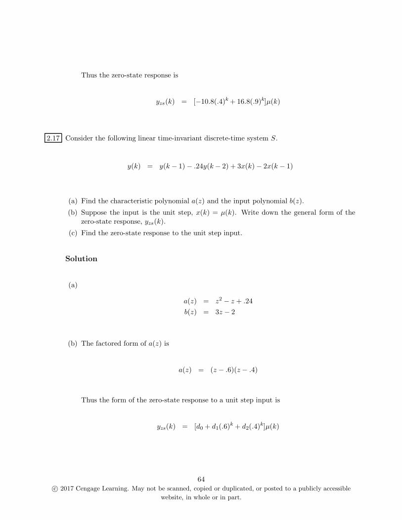
Thus the zero-state response is
yzs(k) = [−10.8(.4)k + 16.8(.9)k]µ(k)
2.17 Consider the following linear time-invariant discrete-time system S.
y(k) = y(k − 1) − .24y(k − 2) + 3x(k) − 2x(k − 1)
(a) Find the characteristic polynomial a(z) and the input polynomial b(z).
(b) Suppose the input is the unit step, x(k) = µ(k). Write down the general form of the
zero-state response, yzs(k).
(c) Find the zero-state response to the unit step input.
Solution
(a)
a(z) = z2 − z + .24
b(z) = 3z − 2
(b) The factored form of a(z) is
a(z) = (z − .6)(z − .4)
Thus the form of the zero-state response to a unit step input is
yzs(k) = [d0 + d1(.6)k + d2(.4)k]µ(k)
64c© 2017 Cengage Learning. May not be scanned, copied or duplicated, or posted to a publicly accessible
website, in whole or in part.

(c)
d0 =Ab(z)
a(z)
∣
∣
∣
∣
z=p0
=3 − 2
(1 − .6)(1− .4)
=1
.24= 4.167
d1 =A(z − p1)b(z)
(z − p0)a(z)
∣
∣
∣
∣
z=p1
=3(.6)− 2
(.6− 1)(.6− .4)
=−.2
−.08= 2.5
d2 =A(z − p2)b(z)
(z − p0)a(z)
∣
∣
∣
∣
z=p2
=3(.4)− 2
(.4− 1)(.4− .6)
=−.8
−.12= 6.667
Thus the zero-state response is
yzs(k) = [4.167 + 2.5(.6)k + 6.667(.4)k]µ(k)
2.18 Consider the following linear time-invariant discrete-time system S.
y(k) = y(k − 1) − .21y(k − 2) + 3x(k) + 2x(k − 2)
(a) Find the characteristic polynomial a(z) and the input polynomial b(z). Express a(z) in
factored form.
(b) Write down the general form of the zero-input response, yzi(k).
(c) Find the zero-input response when the initial condition is y(−1) = 1 and y(−2) = −1.
65c© 2017 Cengage Learning. May not be scanned, copied or duplicated, or posted to a publicly accessible
website, in whole or in part.

(d) Write down the general form of the zero-state response when the input is x(k) =
2(.5)k−1µ(k).
(e) Find the zero-state response using the input in (d).
(f) Find the complete response using the initial condition in (c) and the input in (d).
Solution
(a)
a(z) = z2 − z + .21
= (z − .3)(z − .7)
b(z) = 3z2 + 2
(b) The general form of the zero-input response is
yzi(k) = c1(p1)k + c2(p2)
k
= c1(.3)k + c2(.7)k
(c) Using (b) and applying the initial conditions yields
c1(.3)−1 + c2(.7)−1 = 1
c1(.3)−2 + c2(.7)−2 = −1
Clearing the denominators,
.7c1 + .3c2 = .21
.49c1 + .09c2 = −.0441
Subtracting the second equation from seven times the first equation yields 2.01c2 = 1.51.Subtracting .3 times the first equation from the second yields .28c1 = −.127. Thus the
zero-input response is
yzi(k) = −.454(.3)k + .751(.7)k
66c© 2017 Cengage Learning. May not be scanned, copied or duplicated, or posted to a publicly accessible
website, in whole or in part.

(d) First note that
x(k) = 2(.5)k−1µ(k)
= 4(.5)kµ(k)
The general form of the zero-state response is
yzs(k) = [d0(.5)k + d1(.3)k + d2(.7)k]µ(k)
(e)
d0 =Ab(z)
a(z)
∣
∣
∣
∣
z=p0
=4[3(.5)2 + 2]
(.5− .3)(.5− .7)
=4(2.75)
−.04= −275
d1 =A(z − p1)b(z)
(z − p0)a(z)
∣
∣
∣
∣
z=p1
=4[3(.3)2 + 2]
(.3− .5)(.3− .7)
=4(2.27)
.08= 113.5
d2 =A(z − p2)b(z)
(z − p0)a(z)
∣
∣
∣
∣
z=p2
=4[3(.7)2 + 2]
(.7− .5)(.7− .3)
=4(2.63)
.08= 131.5
Thus the zero-state response is
yzs(k) = [−275(.5)k + 113.5(.3)k + 131.5(.7)k]µ(k)
67c© 2017 Cengage Learning. May not be scanned, copied or duplicated, or posted to a publicly accessible
website, in whole or in part.

(f) By superposition, the complete response is
y(k) = yzi(k) + yzs(k)
= −.454(.3)k + .751(.7)k + [−275(.5)k + 113.5(.3)k + 131.5(.7)k]µ(k)
2.19 Consider the following linear time-invariant discrete-time system S. Sketch a block diagram
of this IIR system.
y(k) = 3y(k − 1) − 2y(k − 2) + 4x(k) + 5x(k − 1)
Solution
a = [1,−3, 2]
b = [4, 5, 0]
x(k) e • •? ? ?
0 5 4
? ? ?
� ��
� ��
� ��
+ + +- -z−1 z−1- - ey(k)
2 −3
6 6− −
6 6
•
•
Problem 2.19
2.20 Consider the following linear time-invariant discrete-time system S. Sketch a block diagramof this FIR system.
y(k) = x(k) − 2x(k − 1) + 3x(k − 2) − 4x(k − 4)
68c© 2017 Cengage Learning. May not be scanned, copied or duplicated, or posted to a publicly accessible
website, in whole or in part.

Solution
a = [1, 0, 0]
b = [1,−2, 3, 0,−4]
x(k) e - z−1 z−1 z−1 z−1- - -• • • •
? ? ? ? ?
? ? ? ?- - - -
� ��
� ��
� ��
� ��
+ + + + ey(k)
1 −2 3 0 −4
Problem 2.20
2.21 Consider the following linear time-invariant discrete-time system S called an auto-regressive
system. Sketch a block diagram of this system.
y(k) = x(k)− .8y(k − 1) + .6y(k − 2)− .4y(k − 3)
Solution
a = [1, .8,−.6, .4]
b = [1, 0, 0, 0]
69c© 2017 Cengage Learning. May not be scanned, copied or duplicated, or posted to a publicly accessible
website, in whole or in part.

x(k) d • • •? ? ? ?0 0 0 1
? ? ? ?m m m m+ + + +- - -z−1 z−1 z−1- - - dy(k)
.4 −.6 .8
6 6 6− − −
6 6 6
•
• •
Problem 2.21
2.22 Consider the block diagram shown in Figure 2.32.
x(k) e • •? ? ?
1.8 .9 −.4
? ? ?
� ��
� ��
� ��
+ + +- -z−1 z−1- -u2(k) u1(k) ey(k)
2.1 −1.5
6 6− −
6 6
•
•
Figure 2.32 A Block Diagram of the System in Problem 2.22
(a) Write a single difference equation description of this system.
(b) Write a system of difference equations for this system for ui(k) for 1 ≤ i ≤ 2 and y(k).
Solution
(a) By inspection of Figure 2.32
y(k) = −.4x(k) + .9x(k − 1) + 1.8x(k − 2) + 1.5y(k − 1) − 2.1y(k − 2)
70c© 2017 Cengage Learning. May not be scanned, copied or duplicated, or posted to a publicly accessible
website, in whole or in part.

(b) The equivalent system of equations is
u2(k) = 1.8x(k)− 2.1y(k)
u1(k) = .9x(k) + 1.5y(k) + u2(k − 1)
y(k) = −.4x(k) + u1(k − 1)
2.23 Consider the following linear time-invariant discrete-time system S.
y(k) = .6y(k − 1) + x(k)− .7x(k − 1)
(a) Find the characteristic polynomial and the input polynomial.
(b) Write down the form of the impulse response, h(k).
(c) Find the impulse response.
Solution
(a)
a(z) = z − .6
b(z) = z − .7
(b)
h(k) = d0δ(k) + d1(.6)kµ(k)
(c)
d0 =b(z)
a(z)
∣
∣
∣
∣
z=0
=−.7)
−.6)
= 1.167
d1 =(z − p1)b(z)
za(z)
∣
∣
∣
∣
z=p1
=.6 − .7)
.6)
= −.167
71c© 2017 Cengage Learning. May not be scanned, copied or duplicated, or posted to a publicly accessible
website, in whole or in part.

Thus the impulse response is
h(k) = 1.167δ(k)− .167(.6)kµ(k)
2.24 Consider the following linear time-invariant discrete-time system S.
y(k) = −.25y(k − 2) + x(k − 1)
(a) Find the characteristic polynomial and the input polynomial.
(b) Write down the form of the impulse response, h(k).
(c) Find the impulse response. Use the identities in Appendix 2 to express h(k) in real form.
Solution
(a)
a(z) = z2 + .25
b(z) = z
(b) First note that
a(z) = (z − .5j)(z + .5j)
Thus the form of the impulse response is
h(k) = d0δ(k) + [d1(.5j)k + d2(−.5j)k]µ(k)
72c© 2017 Cengage Learning. May not be scanned, copied or duplicated, or posted to a publicly accessible
website, in whole or in part.

(c)
d0 =b(z)
a(z)
∣
∣
∣
∣
z=0
= 0
d1 =(z − p1)b(z)
za(z)
∣
∣
∣
∣
z=p1
=.5j)
.5j(j)
= −j
d2 =(z − p2)b(z)
za(z)
∣
∣
∣
∣
z=p2
=−.5j)
−.5j(−j)
= j
Thus from Appendix 2 the impulse response is
h(k) = [−j(.5j)k + j(−.5j)k]µ(k)
= 2Re[−j(.5j)k]µ(k)
= −2Re[(.5)k(j)k+1]µ(k)
= −2(.5)kRe{[exp(jπ/2)]k+1}µ(k)
= −2(.5)kRe[exp[j(k + 1)π/2]µ(k)
= −2(.5)k cos[(k + 1)π/2]µ(k)
2.25 Consider the following linear time-invariant discrete-time system S. Suppose 0 < m ≤ n andthe characteristic polynomial a(z) has simple nonzero roots.
y(k) =
m∑
i=0
bix(k − i)−n
∑
i=1
aiy(k − i)
(a) Find the characteristic polynomial a(z) and the input polynomial b(z).
(b) Find a constraint on b(z) that ensures that the impulse response h(k) does not contain
an impulse term.
Solution
73c© 2017 Cengage Learning. May not be scanned, copied or duplicated, or posted to a publicly accessible
website, in whole or in part.

(a)
a(z) = zn + a1zn−1 + · · ·+ an
b(z) = b0zn + b1z
n−1 + · · ·+ bmzn−m
(b) The coefficient of the impulse term is
d0 =b(z)
a(z)
∣
∣
∣
∣
z=0
=b(0)
a(0)
Thus
d0 6= 0 ⇔ b(0) 6= 0
⇔ m = n
2.26 Consider the following linear time-invariant discrete-time system S. Compute and sketch the
impulse response of this FIR system.
y(k) = u(k − 1) + 2u(k − 2) + 3u(k − 3) + 2u(k − 4) + u(k − 5)
Solution
By inspection, the impulse response is
h(k) = [0, 1, 2, 3, 2, 1, 0, 0, . . .]
74c© 2017 Cengage Learning. May not be scanned, copied or duplicated, or posted to a publicly accessible
website, in whole or in part.

0 1 2 3 4 5 6 70
0.5
1
1.5
2
2.5
3Impulse Response
k
h(k)
Problem 2.26
2.27 Using the definition of linear convolution, show that for any signal h(k)
h(k) ? δ(k) = h(k)
Solution
From Definition 2.3 we have
h(k) ? δ(k) =
∞∑
i=−∞
h(i)x(k − i)
=
∞∑
i=−∞
h(i)δ(k − i)
= h(k)
75c© 2017 Cengage Learning. May not be scanned, copied or duplicated, or posted to a publicly accessible
website, in whole or in part.

2.28 Use Definition 2.3 and the commutative property to show that the linear convolution operator
is associative.
f(k) ? [g(k) ? h(k)] = [f(k) ? g(k)] ? h(k)
Solution
From Definition 2.3 we have
d1(k) = f(k) ? [g(k) ? h(k)]
=∞∑
m=−∞
f(m)
[
∞∑
i=−∞
g(i)h(k− m − i)
]
=
∞∑
m=−∞
∞∑
i=−∞
f(m)g(i)h(k− m − i)
Next, using the commutative property
d2(k) = [f(k) ? g(k)] ? h(k)]
= h(k) ? [f(k) ? g(k)]
=
∞∑
i=−∞
h(i)
[
∞∑
m=−∞
f(m)g(k − i − m)
]
=
∞∑
i=−∞
∞∑
m=−∞
h(i)f(m)g(k− i − m)
=
∞∑
n=−∞
∞∑
m=−∞
h(k − n − m)f(m)g(n) , n = k − i − m
=
∞∑
m=−∞
∞∑
i=−∞
f(m)g(i)h(k− m − i) , i = n
Thus d2(k) = d1(k).
2.29 Use Definition 2.3 to show that the linear convolution operator is distributive.
f(k) ? [g(k) + h(k)] = f(k) ? g(k) + f(k) ? h(k)
76c© 2017 Cengage Learning. May not be scanned, copied or duplicated, or posted to a publicly accessible
website, in whole or in part.

Solution
d(k) = f(k) ? [g(k) + h(k)]
=
∞∑
i=−∞
f(i)[g(k− i) + h(k − i)]
=
∞∑
i=−∞
f(i)g(k − i) + f(i)h(k − i)]
=∞∑
i=−∞
f(i)g(k − i) +∞
∑
i=−∞
f(i)h(k − i)]
= f(k) ? g(k) + f(k) ? h(k)
2.30 Suppose h(k) and x(k) are defined as follows.
h = [2,−1, 0, 4]T
x = [5, 3,−7, 6]T
(a) Let yc(k) = h(k)◦x(k). Find the circular convolution matrix C(x) such that yc = C(x)h.
(b) Use C(x) to find yc(k).
Solution
(a) Using (2.7.9) and Example 2.14 as a guide, the 4 × 4 circular convolution matrix is
C(x) =
x(0) x(3) x(2) x(1)
x(1) x(0) x(3) x(2)x(2) x(1) x(0) x(3)
x(3) x(2) x(1) x(0)
=
5 6 −7 33 5 6 −7
−7 3 5 66 −7 3 5)
77c© 2017 Cengage Learning. May not be scanned, copied or duplicated, or posted to a publicly accessible
website, in whole or in part.

(b) Using (2.7.10) and the results from part (a)
yc = C(x)h
=
5 6 −7 33 5 6 −7
−7 3 5 66 −7 3 5)
2−1
04
=
16
−277
39
This can be verified using the DSP Companion function f conv.
2.31 Suppose h(k) and x(k) are the following signals of length L and M , respectively.
h = [3, 6,−1]T
x = [2, 0,−4, 5]T
(a) Let hz and xz be zero-padded versions of h(k) and x(k) of length N = L + M − 1.Construct hz and xz.
(b) Let yc(k) = hz(k) ◦ xz(k). Find the circular convolution matrix C(xz) such that yc =C(xz)hz.
(c) Use C(xz) to find yc(k).
(d) Use yc(k) to find the linear convolution y(k) = h(k) ? x(k) for 0 ≤ k < N .
Solution
(a) Here
N = L + M − 1
= 3 + 4 − 1
= 6
Thus the zero-padded versions of h(k) and x(k) are
78c© 2017 Cengage Learning. May not be scanned, copied or duplicated, or posted to a publicly accessible
website, in whole or in part.

hz = [3, 6,−1, 0, 0, 0]T
xz = [2, 0,−4, 5, 0, 0]T
(b) Using (2.7.9) and the results from part (a), the N × N circular convolution matrix is
C(xz) =
xz(0) xz(5) xz(4) xz(3) xz(2) xz(1)xz(1) xz(0) xz(5) xz(4) xz(3) xz(2)
xz(2) xz(1) xz(0) xz(5) xz(4) xz(3)xz(3) xz(2) xz(1) xz(0) xz(5) xz(4)
xz(4) xz(3) xz(2) xz(1) xz(0) xz(5)xz(5) xz(4) xz(3) xz(2) xz(1) xz(0)
=
2 0 0 5 −4 0
0 2 0 0 5 −4−4 0 2 0 0 5
5 −4 0 2 0 00 5 −4 0 2 0
0 0 5 −4 0 2
(c) Using (2.7.9), the circular convolution of hz(k) with xz(k) is
yz(k) = C(xz)hz
=
2 0 0 5 −4 00 2 0 0 5 −4−4 0 2 0 0 5
5 −4 0 2 0 00 5 −4 0 2 0
0 0 5 −4 0 2
36−1
00
0
=
612
−14−9
34−5
(d) Using (2.7.14) and the results of part (c), the linear convolution y(k) = h(k) ? x(k) is
y(k) = hz(k) ◦ xz(k)
= C(xz)hz
= [6, 12,−14,−9, 34,−5]T
79c© 2017 Cengage Learning. May not be scanned, copied or duplicated, or posted to a publicly accessible
website, in whole or in part.

This can be verified using the DSP Companion function f conv.
2.32 Consider a linear discrete-time system S with input x and output y. Suppose S is driven by
an input x(k) for 0 ≤ k < L to produce a zero-state output y(k). Use deconvolution to findthe impulse response h(k) for 0 ≤ k < L if x(k) and y(k) are as follows.
x = [2, 0,−1, 4]T
y = [6, 1,−4, 3]T
Solution
Using (2.7.15) and Example 2.16 as a guide
h(0) =y(0)
x(0)
=6
2= 3
Applying (2.7.18) with k = 1 yields
h(1) =y(1)− h(0)x(1)
x(0)
=1 − 3(0)
2= .5
Applying (2.7.18) with k = 2 yields
h(2) =y(2)− h(0)x(2)− h(1)x(1)
x(0)
=−4 − 3(−1)− .5(0)
2= −.5
80c© 2017 Cengage Learning. May not be scanned, copied or duplicated, or posted to a publicly accessible
website, in whole or in part.

Finally, applying (2.7.18) with k = 3 yields
h(3) =y(3)− h(0)x(3)− h(1)x(2)− h(2)x(1)
x(0)
=3 − 3(4)− .5(−1) + .5(0)
2= −4.25
Thus the impulse response of the discrete-time system is
h(k) = [3, .5,−.5,−4.25]T , 0 ≤ k < 4
This can be verified using the DSP Companion function f conv.
2.33 Suppose x(k) and y(k) are the following finite signals.
x = [5, 0,−4]T
y = [10,−5, 7, 4,−12]T
(a) Write the polynomials x(z) and y(z) whose coefficient vectors are x and y, respectively.The leading coefficient corresponds to the highest power of z.
(b) Using long division, compute the quotient polynomial q(z) = y(z)/x(z).
(c) Deconvolve y(k) = h(k) ? x(k) to find h(k), using (2.7.15) and (2.7.18). Compare theresult with q(z) from part (b).
Solution
(a)
x(z) = 5z2 − 4
y(z) = 10z4 − 5z3 + 7z2 + 4z − 12
81c© 2017 Cengage Learning. May not be scanned, copied or duplicated, or posted to a publicly accessible
website, in whole or in part.

(b)
2z2 − z + 3
5z2 − 4 | 10z4 − 5z3 + 7z2 + 4z − 12
10z4 − 0z3 − 8z2
−5z3 + 15z2 + 4z
−5z3 − 0z2 + 4z
15z2 + 0z − 12
15z2 + 0z − 12
0
Thus the quotient polynomial is
q(z) = 2z2 − z + 3
(c) Using (2.7.15) and Example 2.16 as a guide
q(0) =y(0)
x(0)
=−12
−4= 3
Applying (2.7.18) with k = 1 yields
q(1) =y(1)− q(0)x(1)
x(0)
=4 − 3(0)
−4= −1
Applying (2.7.18) with k = 2 yields
q(2) =y(2)− q(0)x(2)− q(1)x(1)
x(0)
=7 − 3(5)− (−1)0
−4= 2
82c© 2017 Cengage Learning. May not be scanned, copied or duplicated, or posted to a publicly accessible
website, in whole or in part.

Thus q = [2,−1, 3] and the quotient polynomial is
q(z) = 2z2 − z + 3
This can be verified using the MATLAB function deconv.
2.34 Some books use the following alternative way to define the linear cross-correlation of an Lpoint signal y(k) with an M -point signal x(k). Using a change of variable, show that this is
equivalent to Definition 2.5
ryx(k) =1
L
L−1−k∑
n=0
y(n + k)x(n)
Solution
Consider the change of variable i = n + k. Then n = i − k and
ryx(k) =1
L
L−1−k∑
n=0
y(n + k)x(n)
∣
∣
∣
∣
∣
i=n+k
=1
L
L−1∑
i=k
y(i)x(i− k)
Since x(n) = 0 for n < 0, the lower limit of the sum can be changed to zero without affectingthe result. Thus,
ryx(k) =1
L
L−1∑
i=0
y(i)x(i− k) , 0 ≤ k < L
This is identical to Definition 2.5.
83c© 2017 Cengage Learning. May not be scanned, copied or duplicated, or posted to a publicly accessible
website, in whole or in part.

2.35 Suppose x(k) and y(k) are defined as follows.
x = [5, 0,−10]T
y = [1, 0,−2, 4, 3]T
(a) Find the linear cross-correlation matrix D(x) such that ryx = D(x)y.
(b) Use D(x) to find the linear cross-correlation ryx(k).
(c) Find the normalized linear cross-correlation ρyx(k).
Solution
(a) Using (2.8.2) and Example 2.18 as a guide, the linear cross-correlation matrix is
D(x) =1
5
x(0) x(1) x(2) 0 0
0 x(0) x(1) x(2) 00 0 x(0) x(1) x(2)
0 0 0 x(0) x(1)0 0 0 0 x(0)
=1
5
5 0 −10 0 0
0 5 0 −10 00 0 5 0 −10
0 0 0 5 00 0 0 0 5
=
1 0 −2 0 0
0 1 0 −2 00 0 1 0 −2
0 0 0 1 00 0 0 0 1
(b) Using (2.8.3) and the results from part (a)
84c© 2017 Cengage Learning. May not be scanned, copied or duplicated, or posted to a publicly accessible
website, in whole or in part.

ryx = D(x)y
=
1 0 −2 0 00 1 0 −2 0
0 0 1 0 −20 0 0 1 00 0 0 0 1
10
−243
=
5−8−8
43
This can be verified using the DSP Companion function f corr.
(c) Using (2.8.5) we have L = 5 and M = 3. Also from Definition 2.5
ryy(0) =1
L
L−1∑
i=0
y2(i)
=1 + 0 + 4 + 16 + 9
5= 6
rxx(0) =1
M
M−1∑
i=0
x2(i)
=25 + 0 + 100
3= 41.67
Finally, from (4.49) the normalized cross-correlation of x(k) with y(k) is
ρyx(k) =ryx(k)
√
(M/L)rxx(0)ryy(0)
=ryx(k)
√
.6(6)41.67
= [.408,−.653,−.653, .327, .245]T
This can be verified using the DSP Companion function f corr.
85c© 2017 Cengage Learning. May not be scanned, copied or duplicated, or posted to a publicly accessible
website, in whole or in part.

√2.36 Suppose y(k) is as follows.
y = [5, 7,−2, 4, 8, 6, 1]T
(a) Construct a 3-point signal x(k) such that ryx(k) reaches its peak positive value at k = 3
and |x(0)| = 1.
(b) Construct a 4-point signal x(k) such that ryx(k) reaches its peak negative value at k = 2
and |x(0)| = 1.
Solution
(a) Recall that the cross-correlation ryx(k) measures the degree which x(k) is similar to asubsignal of y(k). In order for ryx(k) to reach its maximum positive value at k = 3,
one must have maximum positive correlation starting at k = 3. Thus for some positiveconstant α it is necessary that
x = α[y(3), y(4), y(5)]T
= α[4, 8, 6]T
The constraint, |x(0)| = 1, implies that the positive scale factor must be α = 1/4. Thus
x = [1, 2, 1.5]T
(b) In order for ryx(k) to reach its maximum negative value at k = 2, one must havemaximum negative correlation starting at k = 2. Thus for some positive constant α we
need
x = −α[y(2), y(3), y(4), y(5)]T
= α[2,−4,−8,−6]T
The constraint, |x(0)| = 1, implies that the positive scale factor must be α = 1/2. Thus
x = [1,−2,−4,−3]T
The answers to (a) and (b) can be verified using the DSP Companion function f corr.
86c© 2017 Cengage Learning. May not be scanned, copied or duplicated, or posted to a publicly accessible
website, in whole or in part.

2.37 Suppose x(k) and y(k) are defined as follows.
x = [4, 0,−12, 8]T
y = [2, 3, 1,−1]T
(a) Find the circular cross-correlation matrix E(x) such that cyx = E(x)y.
(b) Use E(x) to find the circular cross-correlation cyx(k).
(c) Find the normalized circular cross-correlation σyx(k).
Solution
(a) Using Definition 2.6, cyx(k) is just 1/N times the dot product of y with x rotated rightby k samples. Thus the kth row of E(x) is the vector x rotated right by k samples.
E(x) =1
4
x(0) x(1) x(2) x(3)x(3) x(0) x(1) x(2)
x(2) x(3) x(0) x(1)x(1) x(2) x(3) x(0)
=1
4
4 0 −12 8
8 4 0 −12−12 8 4 0
0 −12 8 4
=
1 0 −3 22 1 0 −3−3 2 1 0
0 −3 2 1
(b) Using Definition 2.6 and the results from part (a)
cyx = E(x)y
=
1 0 −3 22 1 0 −3−3 2 1 0
0 −3 2 1
231
−1
=
−310
1−8
87c© 2017 Cengage Learning. May not be scanned, copied or duplicated, or posted to a publicly accessible
website, in whole or in part.

This can be verified using the DSP Companion function f corr.
(c) Using (2.8.7), N = 4. Also from Definition 2.6
cyy(0) =1
N
N−1∑
i=0
y2(i)
=4 + 9 + 1 + 1
4= 3.75
cxx(0) =1
N
N−1∑
i=0
x2(i)
=16 + 0 + 144 + 64
4= 56
Finally, from (2.8.7) the normalized circular cross-correlation of y(k) with x(k) is
σyx(k) =cyx(k)
√
cxx(0)cyy(0)
=cyx(k)
√
3.75(56)
= [−.207, .690, .069,−.552]T
This can be verified using the DSP Companion function f corr.
2.38 Suppose y(k) is as follows.
y = [8, 2,−3, 4, 5, 7]T
(a) Construct a 6-point signal x(k) such that σyx(2) = 1 and |x(0)| = 6.
(b) Construct a 6-point signal x(k) such that σyx(3) = −1 and |x(0)| = 12.
Solution
88c© 2017 Cengage Learning. May not be scanned, copied or duplicated, or posted to a publicly accessible
website, in whole or in part.

(a) Recall that normalized circular cross-correlation, −1 ≤ σyx(k) ≤ 1, measures the degree
which a rotated version of a signal x(k) is similar to the signal y(k). In order for σyx(k) toreach its maximum positive value at k = 2, one must have maximum positive correlationstarting at k = 2. Thus for some positive constant α it is necessary that
x = α[y(2), y(3), y(4), y(5), y(0), y(1)]T
= α[−3, 4, 5, 7, 8, 2]T
The constraint, |x(0)| = 6, implies that the positive scale factor must be α = 2. Thus
x = [−6, 8, 10, 14, 16, 4]T
Because y and x are of the same length, this will result is σyx(2) = 1 which can beverified by using the DSP Companion function f corr.
(b) In order for σyx(k) to reach its maximum negative value at k = 3, one must have
maximum negative correlation starting at k = 3. Thus for some positive constant α
x = −α[y(3), y(4), y(5), y(0), y(1), y(2)]T
= α[4, 5, 7, 8, 2,−3]T
The constraint, |x(0)| = 12, implies that the positive scale factor must be α = 3. Thus
x = [12, 15, 21, 24, 6,−9]T
Because y and x are of the same length, this will result is σyx(3) = −1 which can beverified by using the DSP Companion function f corr.
2.39 Let x(k) be an N-point signal with average power Px.
(a) Show that rxx(0) = cxx(0) = Px
(b) Show that ρxx(0) = σxx(0) = 1
Solution
89c© 2017 Cengage Learning. May not be scanned, copied or duplicated, or posted to a publicly accessible
website, in whole or in part.

(a) The average power of x(k) is
Px =1
N
N−1∑
k=0
x2(k)
From Definition 2.5, the auto-correlation of an N -point signal is
rxx(0) =1
N
N−1∑
i=0
x(i)x(i− 0)
=1
N
N−1∑
i=0
x2(i)
= Px
From Definition 2.6, the circular auto-correlation of an N -point signal with periodic
extension xp(k) is
cxx(0) =1
N
N−1∑
i=0
x(i)xp(i − 0)
=1
N
N−1∑
i=0
x(i)xp(i)
=1
N
N−1∑
i=0
x2(i)
= Px
(b) From (2.8.5), the normalized auto-correlation of an N -point signal is
ρxx(0) =rxx(0)
√
(N/N )rxx(0)rxx(0)
= 1
From (2.8.7), the normalized circular auto-correlation of an N -point signal is
90c© 2017 Cengage Learning. May not be scanned, copied or duplicated, or posted to a publicly accessible
website, in whole or in part.

σxx(0) =cxx(0)
√
cxx(0)cxx(0)
= 1
2.40 This problem establishes the normalized circular cross-correlation inequality, |σyx(k)| ≤ 1.
Let x(k) and y(k) be sequences of length N where xp(k) is the periodic extension of x(k).
(a) Consider the signal u(i, k) = ay(i) + xp(i− k) where a is arbitrary. Show that
1
N
N−1∑
i=0
[ay(i) + xp(i− k)]2 = a2cyy(0) + 2acyx(k) + cxx(0) ≥ 0
(b) Show that the inequality in part (a) can be written in matrix form as
[a, 1]
[
cyy(0) cyx(k)cyx(k) cxx(0)
] [
a1
]
≥ 0
(c) Since the inequality in part (b) holds for any a, the 2 × 2 coefficient matrix C(k) ispositive semi-definite, which means that det[C(k)] ≥ 0. Use this fact to show that
c2yx(k) ≤ cxx(0)cyy(0) , 0 ≤ k < N
(d) Use the results from part (c) and the definition of normalized cross-correlation to show
that
−1 ≤ σyx(k) ≤ 1 , 0 ≤ k < N
Solution
91c© 2017 Cengage Learning. May not be scanned, copied or duplicated, or posted to a publicly accessible
website, in whole or in part.

(a)
1
N
N−1∑
i=0
u2(i, k) =1
N
N−1∑
i=0
[ay(i) + xp(i− k)]2
=1
N
N−1∑
i=0
a2y2(i) + 2ay(i)xp(i− k) + x2p(i− k)
=a2
N
N−1∑
i=0
y2(i) +2a
N
N−1∑
i=0
y(i)xp(i − k) +1
N
N−1∑
i=0
x2p(i − k)
= a2cyy(0) + 2acyx(k) +1
N
N−1∑
i=0
x2(i)
= a2cyy(0) + 2acyx(k) + cxx(0)
≥ 0
(b)
[a, 1]
[
cyy(0) cyx(k)
cyx(k) cxx(0)
][
a
1
]
= [a, 1]
[
acyy(0) + cyx(k)
acyx(k) + cxx(0)
]
= a2cyy(0) + acyx(k) + acyx(k) + cxx(0)
= a2cyy(0) + 2acyx(k) + cxx(0)
(c) The coefficient matrix C(k) from part (b) is positive semi-definite and therefore det[C(k)] ≥0. But
det[C(k)] = det
{[
cyy(0) cyx(k)cyx(k) cxx(0)
]}
= cyy(0)cxx(0) − c2yx(k)
≥ 0
Thus
c2yx(k) ≤ cxx(0)cyy(0) , 0 ≤ k < N
92c© 2017 Cengage Learning. May not be scanned, copied or duplicated, or posted to a publicly accessible
website, in whole or in part.

(d) Using (2.8.7) and the results from part (c)
|σyx(k)| =
∣
∣
∣
∣
∣
cyx(k)√
cxx(0)cyy(0)
∣
∣
∣
∣
∣
=
∣
∣
∣
∣
∣
√
c2yx(k)
cxx(0)cyy(0)
∣
∣
∣
∣
∣
≤ 1
Thus
−1 ≤ σyx(k) ≤ 1 , 0 ≤ k < N
2.41 Consider the following FIR system.
y(k) =
5∑
i=0
(1 + i)2x(k − i)
Let x(k) be a bounded input with bound Bx. Show that y(k) is bounded with bound By =
cBx. Find the minimum scale factor, c.
Solution
|y(k)| =
∣
∣
∣
∣
∣
5∑
i=0
(1 + i)2x(k − i)
∣
∣
∣
∣
∣
≤5
∑
i=0
|(1 + i)2x(k − i)|
=
5∑
i=0
|(1 + i)2| · |x(k − i)|
≤ Bx
5∑
i=0
|(1 + i)2|
= ‖h‖1Bx
93c© 2017 Cengage Learning. May not be scanned, copied or duplicated, or posted to a publicly accessible
website, in whole or in part.

Here
‖h‖1 =
5∑
i=0
(1 + i)2
= 1 + 4 + 9 + 16 + 25 + 36
= 93
Thus
By = 93Bx
2.42 Consider a linear time-invariant discrete-time system S with the following impulse response.Find conditions on A and p that guarantee that S is BIBO stable.
h(k) = Apkµ(k)
Solution
The system S is BIBO stable if an only if ‖h‖1 < ∞. Here
‖h‖1 =
∞∑
k=−∞
|h(k)|
=
∞∑
k=0
Apk
= A
∞∑
k=0
pk
=A
1 − p, |p| < 1
Thus S is BIBO stable if and only if |p| < 1. There is no constraint on A.
94c© 2017 Cengage Learning. May not be scanned, copied or duplicated, or posted to a publicly accessible
website, in whole or in part.

2.43 From Proposition 2.1, a linear time-invariant discrete-time system S is BIBO stable if and
only if the impulse response h(k) is absolutely summable, that is, ‖h‖1 < ∞. Show that‖h‖1 < ∞ is necessary for stability. That is, suppose that S is stable but h(k) is not absolutelysummable. Consider the following input, where h∗(k) denotes the complex conjugate of h(k)
(Proakis and Manolakis,1992).
x(k) =
h∗(k)
|h(k)| , h(k) 6= 0
0 , h(k) = 0
(a) Show that x(k) is bounded by finding a bound Bx.
(b) Show that S is not is BIBO stable by showing that y(k) is unbounded at k = 0.
Solution
(a) Since x(0) = 0 when h(k) = 0, consider the case when h(k) 6= 0.
|x(k)| =
∣
∣
∣
∣
h∗(k)
|h(k)|
∣
∣
∣
∣
=|h∗(k)||h(k)|
=|h(k)||h(k)|
= 1
Thus x(k) is bounded with Bx = 1.
95c© 2017 Cengage Learning. May not be scanned, copied or duplicated, or posted to a publicly accessible
website, in whole or in part.

(b)
|y(0)| = |h(k) ? x(k)|k=0
=
∣
∣
∣
∣
∣
∞∑
i=−∞
h(i)x(−i)
∣
∣
∣
∣
∣
=
∣
∣
∣
∣
∣
∞∑
i=−∞
h(i)h∗(−i)
|h(−i)|
∣
∣
∣
∣
∣
=
∞∑
i=−∞
|h(i)| · |h∗(−i)||h(−i)|
=
∞∑
i=−∞
|h(i)|
= ‖h‖1
= ∞
2.44 Consider the following discrete-time system. Use GUI module g systime to simulate this
system. Hint: You can enter the b vector in the edit box by using two statements on one line:i=0:8; b=cos(pi*i/4)
y(k) =
8∑
i=0
cos(πi/4)x(k− i)
(a) Plot the polynomial roots
(b) Plot and the impulse response using N = 40.
Solution
96c© 2017 Cengage Learning. May not be scanned, copied or duplicated, or posted to a publicly accessible
website, in whole or in part.

Select type Select view
Slider bar
Edit parameters
0 0.2 0.4 0.6 0.8 10
0.5
1
0 0.2 0.4 0.6 0.8 10
0.5
1
0 0.2 0.4 0.6 0.8 10
0.5
1
−2 −1 0 1 2−2
−1
0
1
2
XXXXXXXXO
O
O
O
O
O
O
O
Polynomial roots: ’x’=a(z), ’o’=b(z)
Re( z)
Im( z)
−2−1
01
2
−2
0
2−20
−10
0
10
20
Re( z)
Magnitude of b(z)/a(z)
Im( z)
|b(z)/a(z)| (dB)
0 0.2 0.4 0.6 0.8 10
0.5
1g_systime
x(k) S y(k)x(k) S y(k)x(k) S y(k)x(k) S y(k)x(k) S y(k)x(k) S y(k)x(k) S y(k)x(k) S y(k)
Problem 2.44 (a) Polynomial Roots
Select type Select view
Slider bar
Edit parameters
0 0.2 0.4 0.6 0.8 10
0.5
1
0 0.2 0.4 0.6 0.8 10
0.5
1
0 5 10 15 20 25 30 350
0.5
1Time signals, unit impulse input
x(k)
0 5 10 15 20 25 30 35−1
0
1
k
y(k)
0 0.2 0.4 0.6 0.8 10
0.5
1g_systime
x(k) S y(k)x(k) S y(k)x(k) S y(k)x(k) S y(k)x(k) S y(k)x(k) S y(k)
Problem 2.44 (b) Impulse Response
97c© 2017 Cengage Learning. May not be scanned, copied or duplicated, or posted to a publicly accessible
website, in whole or in part.

2.45 Consider a discrete-time system with the following characteristic and input polynomials. Use
GUI module g systime to plot the step response using N = 100 points. The MATLAB poly
function can be used to specify coefficient vectors a and b in terms of their roots, as discussedin Section 2.9.
a(z) = (z + .5 ± j.6)(z − .9)(z + .75)
b(z) = 3z2(z − .5)2
Solution
Select type Select view
Slider bar
Edit parameters
0 10 20 30 40 50 60 70 80 900
0.5
1Time signals, unit step input
x(k)
0 10 20 30 40 50 60 70 80 90−5
0
5
k
y(k)
0 0.2 0.4 0.6 0.8 10
0.5
1g_systime
x(k) S y(k)x(k) S y(k)
Problem 2.45 Step Response
98c© 2017 Cengage Learning. May not be scanned, copied or duplicated, or posted to a publicly accessible
website, in whole or in part.

√2.46 Consider the following linear discrete-time system.
y(k) = 1.7y(k − 2) − .72y(k − 4) + 5x(k − 2) + 4.5x(k − 4)
Use GUI module g systime to plot the following damped cosine input and the zero-stateresponse to it using N = 30. To determine F0, set 2πF0kT = .3πk and solve for F0/fs whereT = 1/fs.
x(k) = .97k cos(.3πk)
Solution
2πF0kT = .3πk
Thus 2F0T = .3 or F0 = .15fs. If fs = 2000, then F0 = 300.
99c© 2017 Cengage Learning. May not be scanned, copied or duplicated, or posted to a publicly accessible
website, in whole or in part.

Select type Select view
Slider bar
Edit parameters
0 50 100 150 200 250−1
0
1Time signals, damped cosine input: c=0.97, F0=300
x(k)
0 50 100 150 200 250−10
0
10
20
k
y(k)
0 0.2 0.4 0.6 0.8 10
0.5
1g_systime
x(k) S y(k)x(k) S y(k)
Problem 2.46 Input and Output
2.47 Consider the following linear discrete-time system.
y(k) = −.4y(k − 1) + .19y(k − 2) − .104y(k − 3) + 6x(k) − 7.7x(k − 1) + 2.5x(k − 2)
Create a MAT-file called prob2 47 that contains fs = 100, the appropriate coefficient vectors
a and b, and the following input samples, where v(k) is white noise uniformly distributed over[−.2, .2]. Uniform white noise can be generated with the MATLAB function rand.
x(k) = k exp(−k/50) + v(k) , 0 ≤ k < 500
(a) Print the MATLAB program used to create prob2 47.mat.
(b) Use GUI module g systime and the Import option to plot the roots of the characteristicpolynomial and the input polynomial.
(c) Plot the zero-state response on the input x(k).
100c© 2017 Cengage Learning. May not be scanned, copied or duplicated, or posted to a publicly accessible
website, in whole or in part.

Solution
(a) % Problem 2.47
f_header(’Problem 2.47: Create MAT file’)
fs = 100;
a = [1 .4 -.19 .104]
b = [6 -7.7 2.5];
N = 500;
v = -.2 + .4*rand(1,N);
k = 0:N-1;
x = k .* exp(-k/50) + v;
save prob2_47 fs a b x
what
Select type Select view
Slider bar
−2 −1 0 1 2−2
−1
0
1
2
XX
X
OOO
Polynomial roots: ’x’=a(z), ’o’=b(z)
Re( z)
Im( z)
−2−1
01
2
−2
0
2−100
−50
0
50
Re( z)
Magnitude of b(z)/a(z)
Im( z)
|b(z)/a(z)| (dB)
0 0.2 0.4 0.6 0.8 10
0.5
1g_systime
x(k) S y(k)x(k) S y(k)
Problem 2.47 (b) Polynomial Roots
101c© 2017 Cengage Learning. May not be scanned, copied or duplicated, or posted to a publicly accessible
website, in whole or in part.

Select type Select view
Slider bar
0 0.2 0.4 0.6 0.8 10
0.5
1
0 50 100 150 200 250 300 350 400 450−10
0
10
20Time signals, user−defined input from file prob2_47
x(k)
0 50 100 150 200 250 300 350 400 450−10
0
10
20
k
y(k)
0 0.2 0.4 0.6 0.8 10
0.5
1g_systime
x(k) S y(k)x(k) S y(k)x(k) S y(k)x(k) S y(k)
Problem 2.47 (c) Input and Output
2.48 Consider the following discrete-time system, which is a narrow band resonator filter withsampling frequency of fs = 800 Hz.
y(k) = .704y(k − 1) − .723y(k − 2) + .141x(k)− .141x(k− 2)
Use GUI module g systime to find the zero-input response for the following initial conditions.In each chase plot N = 50 points.
(a) y0 = [10,−3]T
(b) y0 = [−5,−8]T
Solution
102c© 2017 Cengage Learning. May not be scanned, copied or duplicated, or posted to a publicly accessible
website, in whole or in part.

Select type Select view
Slider bar
Edit parameters
0 5 10 15 20 25 30 35 40 45−1
0
1Time signals, zero input
x(k)
0 5 10 15 20 25 30 35 40 45−10
0
10
k
y(k)
0 0.2 0.4 0.6 0.8 10
0.5
1g_systime
x(k) S y(k)x(k) S y(k)
Problem 2.48 (a) Zero-input Response
Select type Select view
Slider bar
Edit parameters
0 0.2 0.4 0.6 0.8 10
0.5
1
0 5 10 15 20 25 30 35 40 45−1
0
1Time signals, zero input
x(k)
0 5 10 15 20 25 30 35 40 45−10
0
10
k
y(k)
0 0.2 0.4 0.6 0.8 10
0.5
1g_systime
x(k) S y(k)x(k) S y(k)x(k) S y(k)x(k) S y(k)
Problem 2.48 (b) Zero-input Response
103c© 2017 Cengage Learning. May not be scanned, copied or duplicated, or posted to a publicly accessible
website, in whole or in part.

2.49 Consider the following discrete-time system, which is a notch filter with sampling interval
T = 1/360 sec.
y(k) = .956y(k− 1)− .914y(k− 2) + x(k)− x(k − 1) + x(k − 2)
Use GUI module g systime to find the output corresponding to the sinusoidal input x(k) =cos(2πF0kT )µ(k). Do the following cases. Use the caliper option to estimate the steady state
amplitude in each case.
(a) Plot the output when F0 = 10 Hz.
(b) Plot the output when F0 = 60 Hz.
Solution
Select type Select view
Slider bar
Edit parameters
0 50 100 150 200 250−1
0
1Time signals, damped cosine input: c=1, F0=10
x(k)
0 50 100 150 200 250−2
0
2
k
y(k)
(x,y) = (143.92,1.06)
0 0.2 0.4 0.6 0.8 10
0.5
1g_systime
x(k) S y(k)x(k) S y(k)
Problem 2.49 (a) F0 = 10 Hz
104c© 2017 Cengage Learning. May not be scanned, copied or duplicated, or posted to a publicly accessible
website, in whole or in part.

Select type Select view
Slider bar
Edit parameters
0 50 100 150 200 250−1
0
1Time signals, damped cosine input: c=1, F0=60
x(k)
0 50 100 150 200 250−1
0
1
k
y(k)
0 0.2 0.4 0.6 0.8 10
0.5
1g_systime
x(k) S y(k)x(k) S y(k)
Problem 2.49 (b) F0 = 60 Hz
2.50 Consider the following two polynomials. Use g systime to compute, plot, and Export to adata file the coefficients of the product polynomial c(z) = a(z)b(z). Then Import the saved
file and display the coefficients of the product polynomial.
a(z) = z2 − 2z + 3
b(z) = 4z3 + 5z2 − 6z + 7
Solution
105c© 2017 Cengage Learning. May not be scanned, copied or duplicated, or posted to a publicly accessible
website, in whole or in part.

Select type Select view
Slider bar
Edit parameters
−1 0 1 2 3 4 5 6−10
0
10
a,b
Convolution
a
b
−1 0 1 2 3 4 5 6−50
0
50conv(a,b)
k
p = a*b
p = a*b
0 0.2 0.4 0.6 0.8 10
0.5
1g_systime
x(k) S y(k)x(k) S y(k)
Problem 2.50 Polynomial Multiplication
product =
4 -3 -4 34 -32 21
2.51 Consider the following two polynomials. Use g systime to compute, plot, and Export to a
data file the coefficients of the quotient polynomial q(z) and the remainder polynomial r(z)where b(z) = q(z)a(z) + r(z). Then Import the saved file and display the coefficients of the
quotient and remainder polynomials.
a(z) = z2 + 3z − 4
b(z) = 4z4 − z2 − 8
Solution
quotient =
4 -12 51
remainder =
0 0 0 -201 196
106c© 2017 Cengage Learning. May not be scanned, copied or duplicated, or posted to a publicly accessible
website, in whole or in part.

Select type Select view
Slider bar
Edit parameters
−1 0 1 2 3 4 5−10
−5
0
5
a,b
Deconvolution
a
b
−1 0 1 2 3 4 5−400
−200
0
200
k
b = q*a + r
q
r
0 0.2 0.4 0.6 0.8 10
0.5
1g_systime
x(k) S y(k)x(k) S y(k)
Problem 2.51 Polynomial Division
√2.52 Use the GUI module g correlate to record the sequence of vowels “A”,“E”,“I”,
“O”,“U” in y. Play y to make sure you have a good recording of all five vowels. Then recordthe vowel “O” in x. Play x back to make sure you have a good recording of “O” that sounds
similar to the “O” in y. Export the results to a MAT-file named my vowels.
(a) Plot the inputs x and y showing the vowels.
(b) Plot the normalized cross-correlation of y with x using the Caliper option to mark thepeak which should show the location of x in y.
(c) Based on the plots in (a), estimate the lag d1 that would be required to get the “O”
in x to align with the “O” in y. Compare this with the peak location d2 in (b). Findthe percent error relative to the estimated lag d1. There will be some error due to the
overlap of x with adjacent vowels and co-articulation effects in creating y.
Solution
107c© 2017 Cengage Learning. May not be scanned, copied or duplicated, or posted to a publicly accessible
website, in whole or in part.

Select type Select view
Slider bar
0 2000 4000 6000 8000 10000 12000 14000 16000−1
0
1Inputs x and y: user−defined inputs from file my_vowels
y(k)
0 2000 4000 6000 8000 10000 12000 14000 16000−1
0
1
k
x(k)
0 0.2 0.4 0.6 0.8 10
0.5
1
x(k)Linear
convolutionx(k)*y(k)
Problem 2.52 (a) The Vowels A, E, I, O, U
Select type Select view
Slider bar
0 0.2 0.4 0.6 0.8 10
0.5
1
0 2000 4000 6000 8000 10000 12000 14000 16000−0.2
−0.1
0
0.1
0.2
0.3Normalized cross−correlation: user−defined inputs from file my_vowels
k
ρyx(k)
0 0.2 0.4 0.6 0.8 10
0.5
1
x(k)
y(k)
Linearcross−
correlation
ρyx(k)
Problem 2.52 (b) Normalized Cross-correlation of x with y
108c© 2017 Cengage Learning. May not be scanned, copied or duplicated, or posted to a publicly accessible
website, in whole or in part.

(c) From part (a), the start of O in x is approximately ox = 9000, and the start of O in y
is approximately oy = 1800. Thus the translation of y required to get a match with x is
d1 = ox − oy
≈ 9000− 1800
= 7200
The peak in part (b) is at d2 = 6807. Thus the percent error in finding the location ofO in x is
E =100(d2 − d1)
d1
=100(6807− 7200)
7200= −5.46 %
2.53 The file prob2 53.mat contains two signals, x and y, and their sampling frequency, fs. Usethe GUI module g correlate to Import x, y, and fs.
(a) Plot x(k) and y(k).
(b) Plot the normalized linear cross-correlation ρyx(k). Does y(k) contain any scaled and
shifted versions of x(k)? Determine how many, and use the Caliper option to estimatethe locations of x(k) within y(k).
Solution
From the plot of ρxy(k), there are three scaled and shifted versions of y(k) within x(k). Theyare located at
k = [388, 1718, 2851]
109c© 2017 Cengage Learning. May not be scanned, copied or duplicated, or posted to a publicly accessible
website, in whole or in part.

Select type Select view
Slider bar
0 0.2 0.4 0.6 0.8 10
0.5
1
0 0.2 0.4 0.6 0.8 10
0.5
1
0 0.2 0.4 0.6 0.8 10
0.5
1
0 500 1000 1500 2000 2500 3000 3500 4000 4500−5
0
5Inputs x and y: user−defined inputs from file prob2_53
y(k)
0 500 1000 1500 2000 2500 3000 3500 4000 4500−1
0
1
k
x(k)
0 0.2 0.4 0.6 0.8 10
0.5
1
x(k)Linear
convolutionx(k)*y(k)
Problem 2.53 (a)
Select type Select view
Slider bar
0 0.2 0.4 0.6 0.8 10
0.5
1
0 500 1000 1500 2000 2500 3000 3500 4000 4500−0.1
−0.05
0
0.05
0.1
0.15
0.2
0.25Normalized cross−correlation: user−defined inputs from file prob2_53
k
ρyx(k)
(x,y) = (385.66,0.19) (x,y) = (1720.47,0.18) (x,y) = (2847.47,0.17)
0 0.2 0.4 0.6 0.8 10
0.5
1
0 0.2 0.4 0.6 0.8 10
0.5
1
x(k)
y(k)
Linearcross−
correlation
ρyx(k)
Problem 2.53 (b)
110c© 2017 Cengage Learning. May not be scanned, copied or duplicated, or posted to a publicly accessible
website, in whole or in part.

2.54 Consider the following discrete-time system.
y(k) = .95y(k − 1) + .035y(k − 2) − .462y(k − 3) + .351y(k − 4) +
.5x(k)− .75x(k − 1)− 1.2x(k − 2) + .4x(k − 3)− 1.2x(k − 4)
Write a MATLAB program that uses filter and plot to compute and plot the zero-state
response of this system to the following input. Plot both the input and the output on thesame graph.
x(k) = (k + 1)2(.8)kµ(k) , 0 ≤ k ≤ 100
Solution
% Problem 2.54
% Initialize
f_header(’Problem 2.54’)
a = [1 -.95 -.035 .462 -.351]
b = [.5 -.75 -1.2 .4 -1.2]
N =101;
k = 0 : N-1;
x = (k+1).^2 .* (.8).^k;
% Find zero-state response
y = filter (b,a,x);
% Plot input and output
figure
h = plot (k,x,k,y);
set (h(2),’LineWidth’,1.0)
f_labels (’’,’k’,’x(k) and y(k)’)
legend (’x’,’y’)
f_wait
111c© 2017 Cengage Learning. May not be scanned, copied or duplicated, or posted to a publicly accessible
website, in whole or in part.

0 20 40 60 80 100−160
−140
−120
−100
−80
−60
−40
−20
0
20
k
x(k) and y(k)
x
y
Problem 2.54 Input and Zero-State Response
2.55 Consider the following discrete-time system.
a(z) = z4 − .3z3 − .57z2 + .115z + .0168
b(z) = 10(z + .5)3
This system has four simple nonzero roots. Therefore the zero-input response consists of asum of the following four natural mode terms.
yzi(k) = c1pk1 + c2p
k2 + c3p
k3 + c4p
k4
The coefficients can be determined from the initial condition
y0 = [y(−1), y(−2), y(−3), y(−4)]T
Setting yzi(−k) = y(−k) for 1 ≤ k ≤ 4 yields the following linear algebraic system in thecoefficient vector c = [c1, c2, c3, c4]
T .
112c© 2017 Cengage Learning. May not be scanned, copied or duplicated, or posted to a publicly accessible
website, in whole or in part.

p−11
p−12
p−13
p−14
p−21
p−22
p−23
p−24
p−31
p−32
p−33
p−34
p−41
p−42
p−43
p−44
c1
c2
c3
c4
= y0
Write a MATLAB program that uses roots to find the roots of the characteristic polynomialand then solves this linear algebraic system for the coefficient vector c using the MATLAB
left division or \ operator when the initial condition is y0. Print the roots and the coefficientvector c. Use stem to plot the zero-input response yzi(k) for 0 ≤ k ≤ 40.
Solution
% Problem 2.55
% Initialize
f_header(’Problem 2.55’)
a = [1 -.3 -.57 .115 .0168]
y = [2 -1 0 3]’
n = 4;
% Construct coefficient matrix
p = roots(a)
A = zeros(n,n);
for i = 1 : n
for k = 1 : n
A(i,k) = p(k)^(-i);
end
end
% Find coefficient vector c
c = A \ y
% Compute zero-input response
N =41;
k = 0 : N-1;
y_0 = zeros(1,N);
for i = 1 : n
113c© 2017 Cengage Learning. May not be scanned, copied or duplicated, or posted to a publicly accessible
website, in whole or in part.

y_0 = y_0 + c(i) .^ k;
end
% Plot it
figure
stem (k,y_0,’filled’,’.’)
f_labels (’’,’k’,’y_0(k)’)
f_wait
Program Output:
p =
-.7000
.8000
.3000
-.1000
c =
-.8195
.8720
-.0742
.0013
0 5 10 15 20 25 30 35 40−0.5
0
0.5
1
1.5
2
2.5
3
3.5
4
k
y0(k)
Problem 2.55 Zero-Input Response to Initial Condition
114c© 2017 Cengage Learning. May not be scanned, copied or duplicated, or posted to a publicly accessible
website, in whole or in part.

√2.56 Consider the discrete-time system in Problem 2.55. Write a MATLAB program that uses the
DSP Companion function f filter0 to compute the zero-input response to the following initialcondition. Use stem to plot the zero-input response yzi(k) for −4 ≤ k ≤ 40.
y0 = [y(−1), y(−2), y(−3), y(−4)]T
Solution
% Problem 2.56
% Initialize
f_header(’Problem 2.56’)
a = [1 -.3 -.57 .115 .0168]
b = 10*poly([-.5,-.5,-.5])
y0 = [2 -1 0 3]’
n = 4;
% Solve system
N = 41;
x = zeros(1,N);
y_zi = f_filter0(b,a,x,y0);
% Plot it
figure
k = [-n : N-1];
stem (k,y_zi,’filled’,’.’)
f_labels (’Zero-input Response’,’k’,’y_{zi}(k)’)
f_wait
115c© 2017 Cengage Learning. May not be scanned, copied or duplicated, or posted to a publicly accessible
website, in whole or in part.

−5 0 5 10 15 20 25 30 35 40−1
−0.5
0
0.5
1
1.5
2
2.5
3Zero−input Response
k
yzi(k)
Problem 2.56 Zero-input Response
2.57 Consider the following running average filter.
y(k) =1
10
9∑
i=0
x(k − i) , 0 ≤ k ≤ 100
Write a MATLAB program that performs the following tasks.
(a) Use filter and plot to compute and plot the zero-state response to the following input,
where v(k) is a random white noise uniformly distributed over [−.1, .1]. Plot x(k) andy(k) below one another. Uniform white noise can be generated using the MATLAB
function rand.
x(k) = exp(−k/20) cos(πk/10)µ(k) + v(k)
(b) Add a third curve to the graph in part (a) by computing and plotting the zero-stateresponse using conv to perform convolution.
Solution
The transfer function of this FIR filter is
116c© 2017 Cengage Learning. May not be scanned, copied or duplicated, or posted to a publicly accessible
website, in whole or in part.

H(z) = .1
9∑
i=0
z−i
% Problem 2.57
% Initialize
f_header(’Problem 2.57’)
m = 9;
b = .1*ones(1,m+1);
a = 1;
N =101;
k = 0 : N-1;
c = .1;
x = exp(-k/20) .* cos(pi*k/10) + f_randu(1,N,-c,c);
% Find zero-state response
y = filter (b,a,x);
% Plot input and output
figure
h = plot (k,x,k,y);
set (h(2),’LineWidth’,1.0)
f_labels (’Input and Output’,’k’,’x(k) and y(k)’)
legend (’x’,’y’)
f_wait
117c© 2017 Cengage Learning. May not be scanned, copied or duplicated, or posted to a publicly accessible
website, in whole or in part.

0 20 40 60 80 100−0.8
−0.6
−0.4
−0.2
0
0.2
0.4
0.6
0.8
1
1.2Input and Output
k
x(k) and y(k)
x
y
Problem 2.57 Running Average Filter of Order m = 9
2.58 Consider the following FIR filter. Write a MATLAB program that performs the following
tasks.
y(k) =20∑
i=0
(−1)ix(k − i)
10 + i2
(a) Use the function filter to compute and plot the impulse response h(k) for 0 ≤ k < N
where N = 50.
(b) Compute and plot the following periodic input.
x(k) = sin(.1πk)− 2 cos(.2πk) + 3 sin(.3πk) , 0 ≤ k < N
(c) Use conv to compute the zero-state response to the input x(k) using convolution. Alsocompute the zero-state response to x(k) using filter. Plot both responses on the same
graph using a legend.
Solution
118c© 2017 Cengage Learning. May not be scanned, copied or duplicated, or posted to a publicly accessible
website, in whole or in part.

% Problem 2.58
% Construct filter
f_header(’Problem 2.58’)
i = 0 : 20;
b = (-1).^2 ./ (10 + i.^2);
a = 1;
% Construct input
N = 50;
k = 0 : N-1;
x = sin(.1*pi*k) - 2*cos(.2*pi*k) + 3*sin(.3*pi*k);
% Compute and plot impulse response
delta = [1,zeros(1,N-1)];
h = filter (b,a,delta);
figure
plot (k,h)
f_labels (’Impulse Response’,’k’,’h(k)’)
f_wait
% Compute and plot zero-state response using convolution
figure
plot (k,x)
f_labels (’Input’,’k’,’x(k)’)
f_wait
circ = 0;
y1 = f_conv (h,x,circ);
k1 = 0 : length(y1)-1;
y2 = filter (b,a,x);
k2 = 0 : N-1;
hp = plot (k1,y1,k2,y2);
set (hp(2),’LineWidth’,1.5)
f_labels (’Zero State Response’,’k’,’y(k)’)
legend (’Using f\_conv’,’Using filter’)
f_wait
119c© 2017 Cengage Learning. May not be scanned, copied or duplicated, or posted to a publicly accessible
website, in whole or in part.

0 10 20 30 40 500
0.01
0.02
0.03
0.04
0.05
0.06
0.07
0.08
0.09
0.1Impulse Response
k
h(k)
Problem 2.58 (a) Impulse Response
0 10 20 30 40 50−5
−4
−3
−2
−1
0
1
2
3
4Input
k
x(k)
Problem 2.58 (b) Periodic Input
120c© 2017 Cengage Learning. May not be scanned, copied or duplicated, or posted to a publicly accessible
website, in whole or in part.

0 20 40 60 80 100−0.8
−0.6
−0.4
−0.2
0
0.2
0.4
0.6
0.8Zero State Response
k
y(k)
Using f_conv
Using filter
Problem 2.58 (c) Zero-State Response
2.59 Consider the following pair of signals.
h = [1, 2, 3, 4, 5, 4, 3, 2, 1]T
x = [2,−1, 3, 4,−5, 0, 7, 9,−6]T
Verify that linear convolution and circular convolution produce different results by writing
a MATLAB program that uses the DSP Companion function f conv to compute the linearconvolution y(k) = h(k) ? x(k) and the circular convolution yc(k) = h(k) ◦ x(k). Plot y(k)
and yc(k) below one another on the same screen.
Solution
% Problem 2.59
% Initialize
f_header(’Problem 2.59’)
h = [1 2 3 4 5 4 3 2 1]
x = [2 -1 3 4 -5 0 7 9 -6]
% Compute convolutions
121c© 2017 Cengage Learning. May not be scanned, copied or duplicated, or posted to a publicly accessible
website, in whole or in part.

y = f_conv (h,x,0);
y_c = f_conv (h,x,1);
% Plot them
figure
subplot (2,1,1)
k = 0 : length(y)-1;
plot (k,y)
f_labels (’Linear Convolution: y(k) = h(k) * x(k)’,’k’,’y(k)’)
subplot (2,1,2)
k = 0 : length(y_c)-1;
plot (k,y_c)
f_labels (’Circular Convolution: y_c(k) = h(k) \circ x(k)’,’k’,’y_c(k)’)
f_wait
0 2 4 6 8 10 12 14 16−20
0
20
40
60Linear Convolution: y(k) = h(k) * x(k)
k
y(k)
0 1 2 3 4 5 6 7 820
30
40
50
60
Circular Convolution: yc(k) = h(k) ° x(k)
k
yc(k)
Problem 2.59 Linear and Circular Convolution
122c© 2017 Cengage Learning. May not be scanned, copied or duplicated, or posted to a publicly accessible
website, in whole or in part.

2.60 Consider the following pair of signals.
h = [1, 2, 4, 8, 16, 8, 4, 2, 1]T
x = [2,−1,−4,−4,−1, 2]T
Verify that linear convolution can be achieved by zero padding and circular convolution bywriting a MATLAB program that pads these signals with an appropriate number of zeros and
uses the DSP Companion function f conv to compare the linear convolution y(k) = h(k)?x(k)with the circular convolution yzc(k) = hz(k) ◦ xz(k). Plot the following.
(a) The zero-padded signals hz(k) and xz(k) on the same graph using a legend.
(b) The linear convolution y(k) = h(k) ? x(k).
(c) The zero-padded circular convolution yzc(k) = hz(k) ◦ xz(k).
Solution
% Problem 2.60
% Initialize
f_header(’Problem 2.60’)
h = [1 2 4 8 16 8 4 2 1];
x = [2 -1 -4 -4 -1 2];
% Construct and plot zero-padded signals
L = length(h);
M = length(x);
h_z = [h, zeros(1,M-1)]
x_z = [x, zeros(1,L-1)]
figure
k = 0 : length(h_z)-1;
hp = plot (k,h_z,k,x_z);
set (hp(1),’LineWidth’,1.5)
f_labels (’Zero-Padded Signals’,’k’,’Inputs’)
legend (’h_z(k)’,’x_z(k)’)
f_wait
% Compute and plot convolutions
123c© 2017 Cengage Learning. May not be scanned, copied or duplicated, or posted to a publicly accessible
website, in whole or in part.

y = f_conv (h,x,0);
y_zc = f_conv (h_z,x_z,1);
figure
plot (k,y)
f_labels (’Linear Convolution: y(k) = h(k) * x(k)’,’k’,’y(k)’)
f_wait
figure
plot (k,y_zc)
f_labels (’Circular Convolution: y_{zc}(k) = h_z(k) \circ x_z(k)’,’k’,’y_{zc}(k)’)
f_wait
0 2 4 6 8 10 12 14−4
−2
0
2
4
6
8
10
12
14
16Zero−Padded Signals
k
Inputs
hz(k)
xz(k)
Problem 2.60 (a) Zero-padded Signals
124c© 2017 Cengage Learning. May not be scanned, copied or duplicated, or posted to a publicly accessible
website, in whole or in part.

0 2 4 6 8 10 12 14−100
−80
−60
−40
−20
0
20Linear Convolution: y(k) = h(k) * x(k)
k
y(k)
Problem 2.60 (b) Linear Convolution
0 2 4 6 8 10 12 14−100
−80
−60
−40
−20
0
20
Circular Convolution: yzc(k) = h
z(k) ° x
z(k)
k
yzc(k)
Problem 2.60 (c) Zero-padded Circular Convolution
125c© 2017 Cengage Learning. May not be scanned, copied or duplicated, or posted to a publicly accessible
website, in whole or in part.

2.61 Consider the following polynomials
a(z) = z4 + 4z3 + 2z2 − z + 3
b(z) = z3 − 3z2 + 4z − 1
c(z) = a(z)b(z)
Let a ∈ R5, b ∈ R4 and c ∈ R8 be the coefficient vectors of a(z), b(z) and c(z), respectively.
(a) Find the coefficient vector of c(z) by direct multiplication by hand.
(b) Write a MATLAB program that uses conv to find the coefficient vector of c(z) by com-puting c as the linear convolution of a with b.
(c) In the program, show that a can be recovered from b and c by using the MATLAB
function deconv to perform deconvolution.
Solution
% Problem 2.61
% Initialize
f_header(’Problem 2.61’)
a = [1 4 2 -1 3]
b = [1 -3 4 -1]
% Construct coefficient vector of product polynomial
c = conv (a,b)
% Recover coefficients of a from b and c
[a,r] = deconv (c,a)
(a) Using direct multiplication, C(z) = A(z)B(z), we have
126c© 2017 Cengage Learning. May not be scanned, copied or duplicated, or posted to a publicly accessible
website, in whole or in part.

A(z)B(z) = z4 + 4z3 + 2z2 − z + 3
z3 − 3z2 + 4z − 1
z7 + 4z6 + 2z5 − z4 + 3z3
−3z6 − 12z5 − 6z4 + 3z3 − 9z2
4z5 + 16z4 + 8z3 − 4z2 + 12z
−z4 − 4z3 − 2z2 + z − 3
z7 + z6 − 6z5 + 8z4 + 10z3 − 15z2 + 13z − 3
Thus the coefficient vector of the product polynomial is
c = [1, 1,−6, 8, 10,−15, 13,−3]T
(b) The program output for c using conv is
c =
1 1 -6 8 10 -15 13 -3
(c) The program output for a using deconv is
a =
1 -3 4 -1
2.62 Consider the following pair of signals.
x = [2,−4, 3, 7, 6, 1, 9, 4,−3, 2, 7, 8]T
y = [3, 2, 1, 0,−1,−2,−3,−2,−1, 0, 1, 2]T
Verify that linear cross-correlation and circular cross-correlation produce different results bywriting a MATLAB program that uses the DSP Companion function f corr to compute the
linear cross-correlation, ryx(k), and the circular cross-correlation, cyx(k). Plot ryx(k) andcyx(k) below one another on the same screen.
Solution
127c© 2017 Cengage Learning. May not be scanned, copied or duplicated, or posted to a publicly accessible
website, in whole or in part.

% Problem 2.62
% Initialize
f_header(’Problem 2.62’)
x = [3 2 1 0 -1 -2 -3 -2 -1 0 1 2]
y = [2 -4 3 7 6 1 9 4 -3 2 7 8]
% Compute cross-correlations
r_xy = f_corr (x,y,0,0);
c_xy = f_corr (x,y,1,0);
% Plot them
figure
subplot (2,1,1)
k = 0 : length(r_xy)-1;
plot (k,r_xy)
f_labels (’Linear Cross-Correlation’,’k’,’r_{xy}(k)’)
subplot (2,1,2)
k = 0 : length(c_xy)-1;
plot (k,c_xy)
f_labels (’Circular Cross-Correlation)’,’k’,’c_{xy}(k)’)
f_wait
128c© 2017 Cengage Learning. May not be scanned, copied or duplicated, or posted to a publicly accessible
website, in whole or in part.

0 2 4 6 8 10 12−4
−2
0
2Linear Cross−Corrlation
k
rxy(k)
0 5 10 15−4
−2
0
2
4Circular Cross−Correlation)
k
cxy(k)
Problem 2.62 Linear and Circular Cross-Correlation
√2.63 Consider the following pair of signals.
y = [1, 8,−3, 2, 7,−5,−1, 4]T
x = [2,−3, 4, 0, 5]T
Verify that linear cross-correlation can be achieved by zero-padding and circular cross-correlation
by writing a MATLAB program that pads these signals with an appropriate number of zerosand uses the DSP Companion function f corr to compute the linear cross-correlation ryx(k)
and the circular cross-correlation cyzxz(k). Plot the following.
(a) The zero-padded signals xz(k) and yz(k) on the same graph using a legend.
(b) The linear cross-correlation ryx(k) and the scaled zero-padded circular cross-correlation
(N/L)cyzxz(k) on the same graph using a legend.
Solution
% Problem 2.63
129c© 2017 Cengage Learning. May not be scanned, copied or duplicated, or posted to a publicly accessible
website, in whole or in part.

% Initialize
f_header(’Problem 2.63’)
y = [1 8 -3 2 7 -5 -1 4]
x = [2 -3 4 0 5]
% Construct and plot zero-padded signals
L = length(y);
M = length(x);
x_z = [x, zeros(1,L-1)];
y_z = [y, zeros(1,M-1)];
figure
N = length(y_z);
k = 0 : N-1;
hp = plot (k,x_z,k,y_z);
set (hp(1),’LineWidth’,1.5)
f_labels (’Zero-Padded Signals’,’k’,’Inputs’)
legend (’x_z(k)’,’y_z(k)’)
f_wait
% Compute and plot cross-correlations
r_yx = f_corr (y,x,0,0);
R_yx = (N/L)*f_corr (y_z,x_z,1,0);
kr = 0 : length(r_yx)-1;
kR = 0 : length(R_yx)-1;
figure
h = plot (kR,R_yx,kr,r_yx);
set (h(2),’LineWidth’,1.5)
legend (’(N/L)c_{y_zx_z}(k)’, ’r_{yx}(k)’,’Location’,’North’)
f_wait
130c© 2017 Cengage Learning. May not be scanned, copied or duplicated, or posted to a publicly accessible
website, in whole or in part.

0 2 4 6 8 10 12−6
−4
−2
0
2
4
6
8Zero−Padded Signals
k
Inputs
xz(k)
yz(k)
Problem 2.63 (a) Zero-Padded Signals
0 5 10 15−3
−2
−1
0
1
2
3
4
5
(N/L)cy
zx
z
(k)
ryx
(k)
Problem 2.63 (b) Cross-Correlations
131c© 2017 Cengage Learning. May not be scanned, copied or duplicated, or posted to a publicly accessible
website, in whole or in part.

2.64 Consider the following pair of signals of length N = 8.
x = [2,−4, 7, 3, 8,−6, 5, 1]T
y = [3, 1,−5, 2, 4, 9, 7, 0]T
Write a MATLAB program that performs the following tasks.
(a) Use the DSP Companion function f corr to compute the circular cross-correlation, cyx(k).
(b) Compute and print u(k) = x(−k) using the periodic extension, xp(k).
(c) Verify that cyx(k) = [y(k) ◦ x(−k)]/N by using the DSP Companion function f conv to
compute and plot the scaled circular convolution, w(k) = [u(k) ◦ x(k)]/N . Plot cyx(k)and w(k) below one another on the same screen.
Solution
% Problem 2.64
% Initialize
f_header(’Problem 2.64’)
y = [3 1 -5 2 4 9 7 0]
x = [2 -4 7 3 8 -6 5 1]
% Compute and plot circular cross-correlation
c_yx = f_corr (y,x,1,0);
% Construct u(k) = x(-k) using periodic extension x_p(k)
N = length(x);
u = [x(1), x(N:-1:2)]
% Compute and plot scaled circular convolution
w = f_conv (y,u,1)/N;
figure
subplot(2,1,1)
kc = 0 : length(c_yx)-1;
plot (kc,c_yx)
f_labels (’Circular Cross-correlation of y(k) with x(k)’,’k’,’c_{yx}(k)’)
132c© 2017 Cengage Learning. May not be scanned, copied or duplicated, or posted to a publicly accessible
website, in whole or in part.

subplot(2,1,2)
kw = 0 : length(w)-1;
plot (kw,w)
f_labels (’Scaled Circular Convolution of y(k) with x(-k)’,’k’,’[y(k) \circ x(-k)]/N’)
f_wait
(b) The signal u(k) = x(−k) using the periodic extension xp(k) is
u =
2 1 5 -6 8 3 7 -4
0 1 2 3 4 5 6 7−5
0
5
10
15Circular Cross−correlation of y(k) with x(k)
k
cyx(k)
0 1 2 3 4 5 6 7−5
0
5
10
15Scaled Circular Convolution of y(k) with x(−k)
k
[y(k)
° x(−k)]/N
Problem 2.64 (c) Scaled Circular Convolution
133c© 2017 Cengage Learning. May not be scanned, copied or duplicated, or posted to a publicly accessible
website, in whole or in part.

134c© 2017 Cengage Learning. May not be scanned, copied or duplicated, or posted to a publicly accessible
website, in whole or in part.
Digital Signal Processing using MATLAB 3rd Edition Schilling Solutions ManualFull Download: http://testbanklive.com/download/digital-signal-processing-using-matlab-3rd-edition-schilling-solutions-manual/
Full download all chapters instantly please go to Solutions Manual, Test Bank site: testbanklive.com
Related Documents