Digital Signal Processing Knowledge booklet

Unrestricted

Digital Signal Processing Knowledge booklet

Testing Knowledge Base compilation

https://community.plm.automation.siemens.com/

1

Unrestricted

Table of Contents Digital Signal Processing ................................................................................................................................ 0

Knowledge booklet ....................................................................................................................................... 0

Digital Signal Processing ................................................................................................................................ 2

Gain, Range, and Quantization ................................................................................................................... 11

Aliasing ........................................................................................................................................................ 19

Overloads .................................................................................................................................................... 24

Averaging Types: What’s the Difference? ................................................................................................... 32

Spectrum Versus Autopower ...................................................................................................................... 37

The Auto-Power Function ........................................................................................................................... 48

What is a Power Spectral Density (PSD)? ................................................................................................... 57

Windows and Spectral Leakage .................................................................................................................. 66

Window Types ............................................................................................................................................. 75

Window Correction Factors ........................................................................................................................ 88

Root Mean Square (RMS) and Overall Level ............................................................................................... 94

The Gibbs Phenomenon ............................................................................................................................ 107

Introduction to Filters: FIR versus IIR ........................................................................................................ 117

All Articles - Siemens PLM Community Testing Knowledge Base ................................................................. 0

The content in this booklet and the Siemens PLM Community site is the hard work and dedication of many individuals. The Siemens PLM Community site can be found at: https://community.plm.automation.siemens.com/

2

Unrestricted

Digital Signal Processing

During digital data acquisition, transducers output analog signals which must be digitized for a computer. A computer cannot store continuous analog time waveforms like the transducers produce, so instead it breaks the signal into discrete ‘pieces’ or ‘samples’ to store them. Data is recorded in the time domain, but often it is desired to perform a Fourier transform to view the data in the frequency domain. There are unique terms used when performing a Fourier transform on this digitized data, which are not always used in the analog case. They are listed in Figure 1 below:

Figure 1: Time domain and frequency domain terms used in performing a digital Fourier

transform Whether viewing digital data in the time domain or in the frequency domain, understanding the relationship between these different terms affects the quality of the final analysis.

3

Unrestricted

Time Domain Terms

Sampling Rate (Fs) – Number of data samples acquired per second

Frame Size (T) – Amount of time data collected to perform a Fourier transform

Block Size (N) – Total number of data samples acquired during one frame

Frequency Domain Terms

Bandwidth (Fmax) – Highest frequency that is captured in the Fourier transform, equal to half the sampling rate

Spectral Lines (SL)– After Fourier transform, total number of frequency domain samples

Frequency Resolution (Δf) – Spacing between samples in the frequency domain

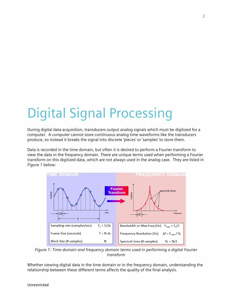
Sampling Rate (Fs) Sampling rate (sometimes called sampling frequency or Fs) is the number of data points acquired per second. A sampling rate of 2000 samples/second means that 2000 discrete data points are acquired every second. This can be referred to as 2000 Hertz sample frequency. The sampling rate is important for determining the maximum amplitude and correct waveform of the signal as shown in Figure 2.

Figure 2: In the top graph, the 10 Hertz sine wave sampled at 1000 samples/second has correct

amplitude and waveform. In the other plots, lower sample rates do not yield the correct amplitude nor shape of the sine wave

To get close to the correct peak amplitude in the time domain, it is important to sample at least 10 times faster than the highest frequency of interest. For a 100 Hertz sine wave, the minimum

4

Unrestricted

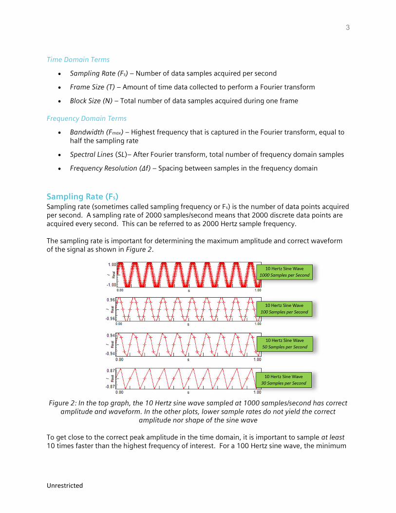
sampling rate would be 1000 samples per second. In practice, sampling even higher than 10x helps measure the amplitude correctly in the time domain. It should be noted that obtaining the correct amplitude in the frequency domain only requires sampling twice the highest frequency of interest. In practice, the anti-aliasing filter in most data acquisition systems makes the requirement 2.5 times the frequency of interest. The Bandwidth section contains more information about the anti-aliasing filter. The inverse of sampling frequency (Fs) is the sampling interval or Δt. It is the amount of time between data samples collected in the time domain as shown in Figure 3.

Figure 3: Sampling frequency and sampling interval relationship

The smaller the quantity Δt, the better the chance of measuring the true peak in the time domain.

Block Size (N) The block size (N) is the total number of time data points that are captured to perform a Fourier transform. A block size of 2000 means that two thousand data points are acquired, then a Fourier transform is performed.

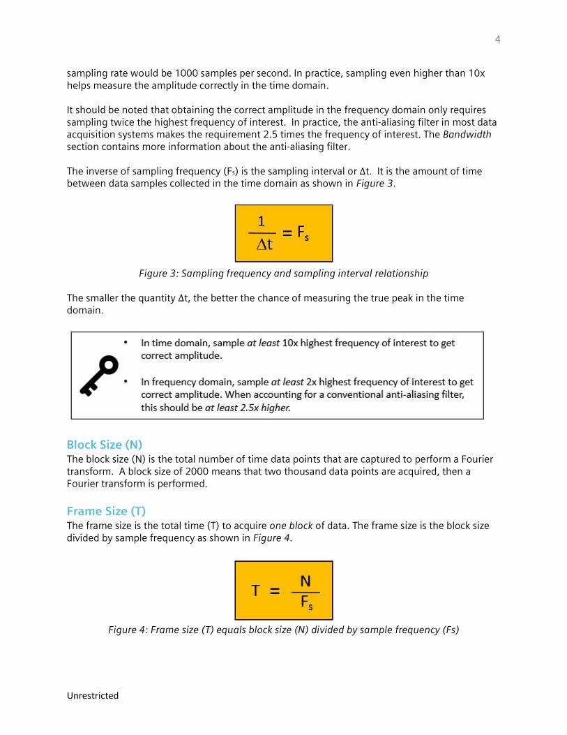
Frame Size (T) The frame size is the total time (T) to acquire one block of data. The frame size is the block size divided by sample frequency as shown in Figure 4.

Figure 4: Frame size (T) equals block size (N) divided by sample frequency (Fs)

5

Unrestricted

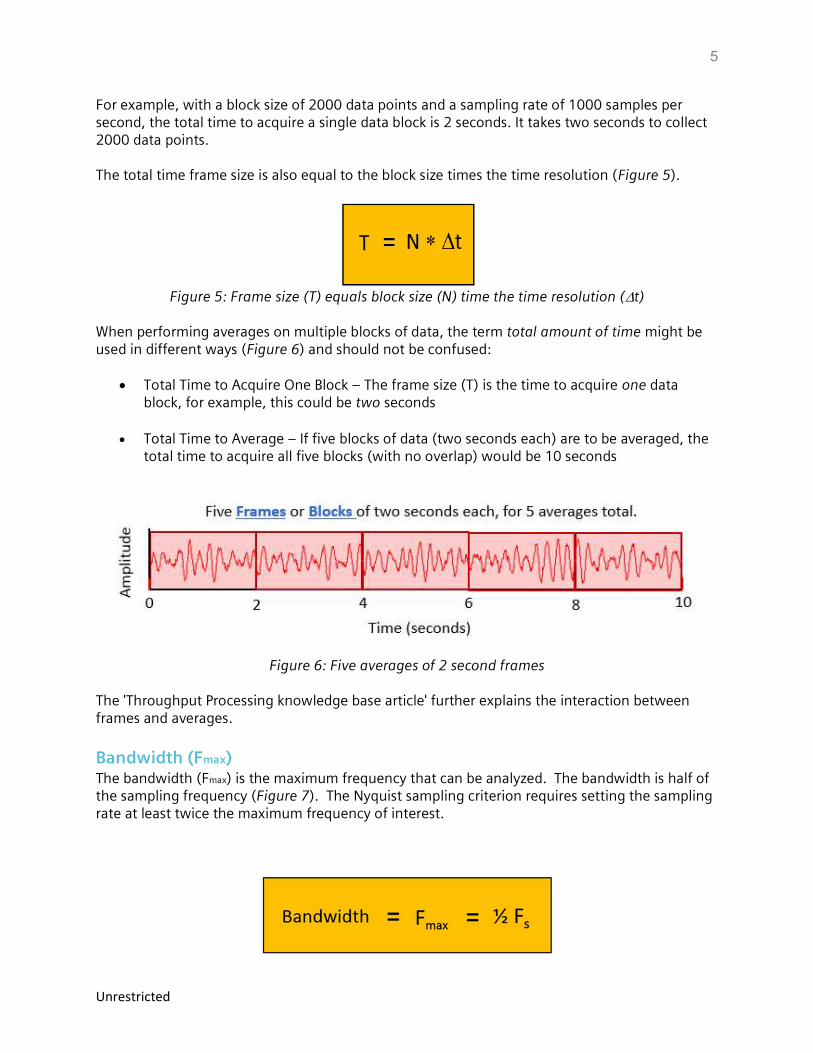
For example, with a block size of 2000 data points and a sampling rate of 1000 samples per second, the total time to acquire a single data block is 2 seconds. It takes two seconds to collect 2000 data points. The total time frame size is also equal to the block size times the time resolution (Figure 5).

Figure 5: Frame size (T) equals block size (N) time the time resolution (t)

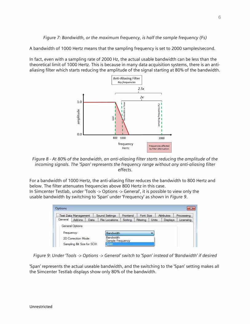
When performing averages on multiple blocks of data, the term total amount of time might be used in different ways (Figure 6) and should not be confused:

Total Time to Acquire One Block – The frame size (T) is the time to acquire one data block, for example, this could be two seconds

Total Time to Average – If five blocks of data (two seconds each) are to be averaged, the total time to acquire all five blocks (with no overlap) would be 10 seconds

Figure 6: Five averages of 2 second frames

The 'Throughput Processing knowledge base article' further explains the interaction between frames and averages.

Bandwidth (Fmax) The bandwidth (Fmax) is the maximum frequency that can be analyzed. The bandwidth is half of the sampling frequency (Figure 7). The Nyquist sampling criterion requires setting the sampling rate at least twice the maximum frequency of interest.

6

Unrestricted

Figure 7: Bandwidth, or the maximum frequency, is half the sample frequency (Fs)

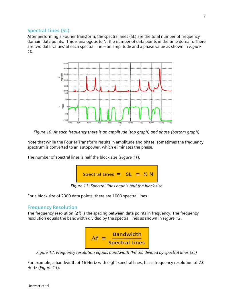
A bandwidth of 1000 Hertz means that the sampling frequency is set to 2000 samples/second. In fact, even with a sampling rate of 2000 Hz, the actual usable bandwidth can be less than the theoretical limit of 1000 Hertz. This is because in many data acquisition systems, there is an anti-aliasing filter which starts reducing the amplitude of the signal starting at 80% of the bandwidth.

Figure 8 - At 80% of the bandwidth, an anti-aliasing filter starts reducing the amplitude of the

incoming signals. The 'Span' represents the frequency range without any anti-aliasing filter effects.

For a bandwidth of 1000 Hertz, the anti-aliasing filter reduces the bandwidth to 800 Hertz and below. The filter attenuates frequencies above 800 Hertz in this case. In Simcenter Testlab, under ‘Tools -> Options -> General’, it is possible to view only the usable bandwidth by switching to ‘Span’ under ‘Frequency’ as shown in Figure 9.

Figure 9: Under ‘Tools -> Options -> General’ switch to ‘Span’ instead of ‘Bandwidth’ if desired ‘Span’ represents the actual useable bandwidth, and the switching to the ‘Span’ setting makes all the Simcenter Testlab displays show only 80% of the bandwidth.

7

Unrestricted

Spectral Lines (SL) After performing a Fourier transform, the spectral lines (SL) are the total number of frequency domain data points. This is analogous to N, the number of data points in the time domain. There are two data ‘values’ at each spectral line – an amplitude and a phase value as shown in Figure 10.

Figure 10: At each frequency there is an amplitude (top graph) and phase (bottom graph)

Note that while the Fourier Transform results in amplitude and phase, sometimes the frequency spectrum is converted to an autopower, which eliminates the phase. The number of spectral lines is half the block size (Figure 11).

Figure 11: Spectral lines equals half the block size

For a block size of 2000 data points, there are 1000 spectral lines.

Frequency Resolution The frequency resolution (Δf) is the spacing between data points in frequency. The frequency resolution equals the bandwidth divided by the spectral lines as shown in Figure 12.

Figure 12: Frequency resolution equals bandwidth (Fmax) divided by spectral lines (SL)

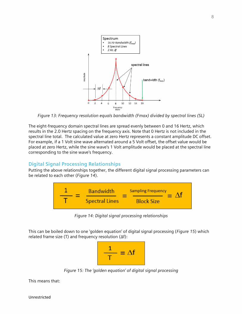
For example, a bandwidth of 16 Hertz with eight spectral lines, has a frequency resolution of 2.0 Hertz (Figure 13).

8

Unrestricted

Figure 13: Frequency resolution equals bandwidth (Fmax) divided by spectral lines (SL)

The eight-frequency domain spectral lines are spread evenly between 0 and 16 Hertz, which results in the 2.0 Hertz spacing on the frequency axis. Note that 0 Hertz is not included in the spectral line total. The calculated value at zero Hertz represents a constant amplitude DC offset. For example, if a 1 Volt sine wave alternated around a 5 Volt offset, the offset value would be placed at zero Hertz, while the sine wave's 1 Volt amplitude would be placed at the spectral line corresponding to the sine wave's frequency.

Digital Signal Processing Relationships Putting the above relationships together, the different digital signal processing parameters can be related to each other (Figure 14).

Figure 14: Digital signal processing relationships

This can be boiled down to one ‘golden equation’ of digital signal processing (Figure 15) which related frame size (T) and frequency resolution (Δf):

Figure 15: The ‘golden equation’ of digital signal processing

This means that:

9

Unrestricted

The finer the desired frequency resolution, the longer the acquisition time The shorter the acquisition time, or frame size, the coarser the frequency resolution

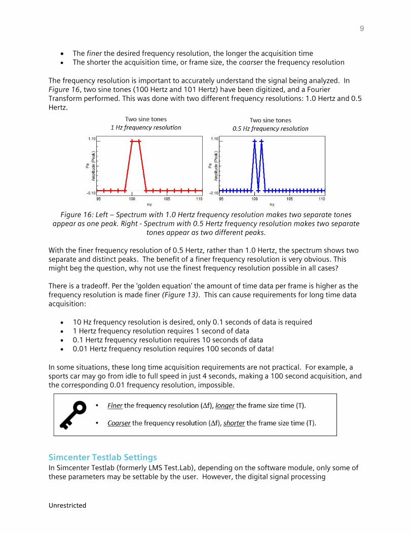
The frequency resolution is important to accurately understand the signal being analyzed. In Figure 16, two sine tones (100 Hertz and 101 Hertz) have been digitized, and a Fourier Transform performed. This was done with two different frequency resolutions: 1.0 Hertz and 0.5 Hertz.

Figure 16: Left – Spectrum with 1.0 Hertz frequency resolution makes two separate tones

appear as one peak. Right - Spectrum with 0.5 Hertz frequency resolution makes two separate tones appear as two different peaks.

With the finer frequency resolution of 0.5 Hertz, rather than 1.0 Hertz, the spectrum shows two separate and distinct peaks. The benefit of a finer frequency resolution is very obvious. This might beg the question, why not use the finest frequency resolution possible in all cases? There is a tradeoff. Per the ‘golden equation’ the amount of time data per frame is higher as the frequency resolution is made finer (Figure 13). This can cause requirements for long time data acquisition:

10 Hz frequency resolution is desired, only 0.1 seconds of data is required 1 Hertz frequency resolution requires 1 second of data 0.1 Hertz frequency resolution requires 10 seconds of data 0.01 Hertz frequency resolution requires 100 seconds of data!

In some situations, these long time acquisition requirements are not practical. For example, a sports car may go from idle to full speed in just 4 seconds, making a 100 second acquisition, and the corresponding 0.01 frequency resolution, impossible.

Simcenter Testlab Settings In Simcenter Testlab (formerly LMS Test.Lab), depending on the software module, only some of these parameters may be settable by the user. However, the digital signal processing

10

Unrestricted

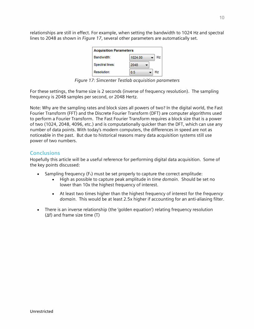
relationships are still in effect. For example, when setting the bandwidth to 1024 Hz and spectral lines to 2048 as shown in Figure 17, several other parameters are automatically set.

Figure 17: Simcenter Testlab acquisition parameters

For these settings, the frame size is 2 seconds (inverse of frequency resolution). The sampling frequency is 2048 samples per second, or 2048 Hertz. Note: Why are the sampling rates and block sizes all powers of two? In the digital world, the Fast Fourier Transform (FFT) and the Discrete Fourier Transform (DFT) are computer algorithms used to perform a Fourier Transform. The Fast Fourier Transform requires a block size that is a power of two (1024, 2048, 4096, etc.) and is computationally quicker than the DFT, which can use any number of data points. With today’s modern computers, the differences in speed are not as noticeable in the past. But due to historical reasons many data acquisition systems still use power of two numbers.

Conclusions Hopefully this article will be a useful reference for performing digital data acquisition. Some of the key points discussed:

Sampling frequency (Fs) must be set properly to capture the correct amplitude: High as possible to capture peak amplitude in time domain. Should be set no

lower than 10x the highest frequency of interest.

At least two times higher than the highest frequency of interest for the frequency domain. This would be at least 2.5x higher if accounting for an anti-aliasing filter.

There is an inverse relationship (the ‘golden equation’) relating frequency resolution (Δf) and frame size time (T)

11

Unrestricted

Gain, Range, and Quantization

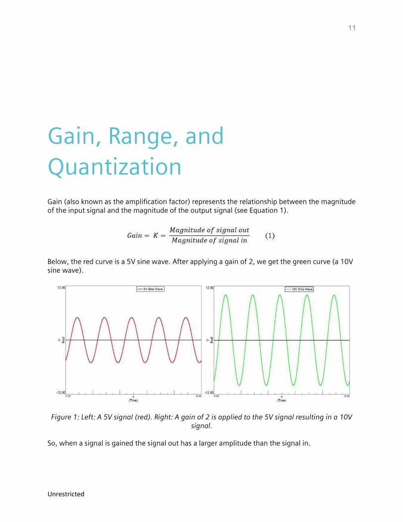
Gain (also known as the amplification factor) represents the relationship between the magnitude of the input signal and the magnitude of the output signal (see Equation 1).

Below, the red curve is a 5V sine wave. After applying a gain of 2, we get the green curve (a 10V sine wave).

Figure 1: Left: A 5V signal (red). Right: A gain of 2 is applied to the 5V signal resulting in a 10V signal.

So, when a signal is gained the signal out has a larger amplitude than the signal in.

12

Unrestricted

How is a Signal Gained? Signals are gained by using an amplifier (amp). An amplifier is an electronic component that boosts electronic signals. Amplifiers come in many shapes, sizes, and types, but all exhibit the property of gain. Below are two examples of amplifiers, a tiny transistor amplifier and a large guitar amplifier. TIP33C Transistor Fender Champion 20 Combo Guitar Amplifier

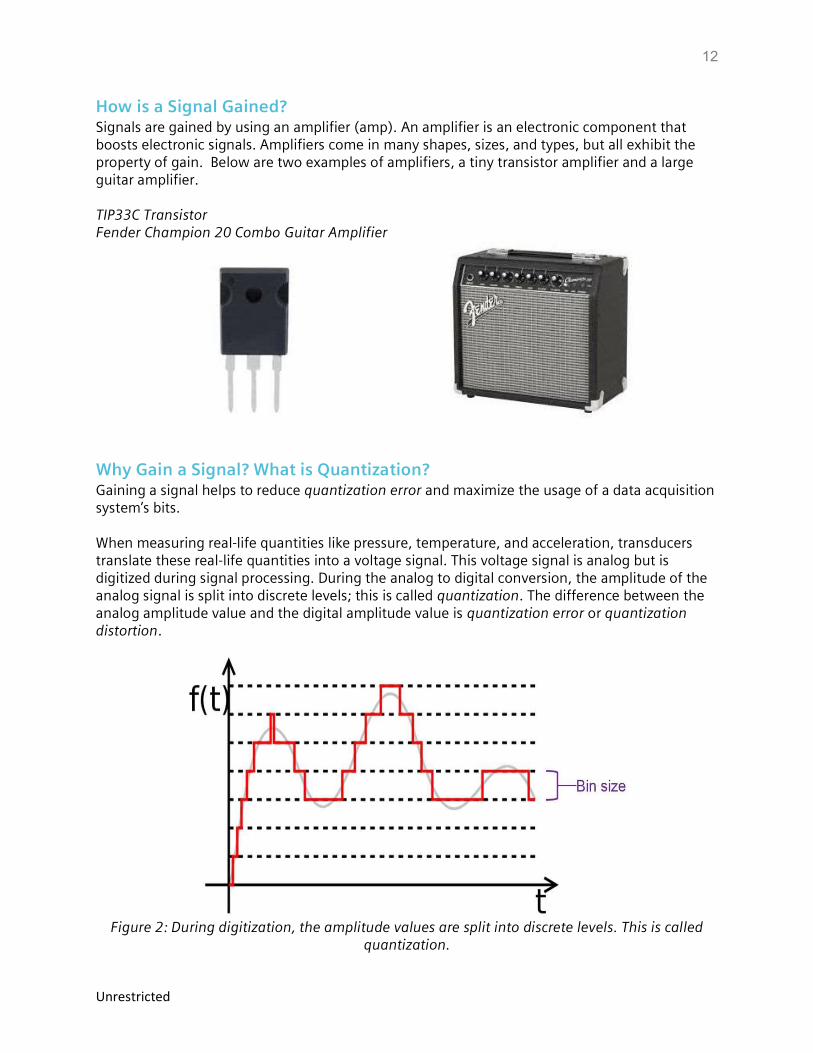
Why Gain a Signal? What is Quantization? Gaining a signal helps to reduce quantization error and maximize the usage of a data acquisition system’s bits. When measuring real-life quantities like pressure, temperature, and acceleration, transducers translate these real-life quantities into a voltage signal. This voltage signal is analog but is digitized during signal processing. During the analog to digital conversion, the amplitude of the analog signal is split into discrete levels; this is called quantization. The difference between the analog amplitude value and the digital amplitude value is quantization error or quantization distortion.

Figure 2: During digitization, the amplitude values are split into discrete levels. This is called

quantization.

13

Unrestricted

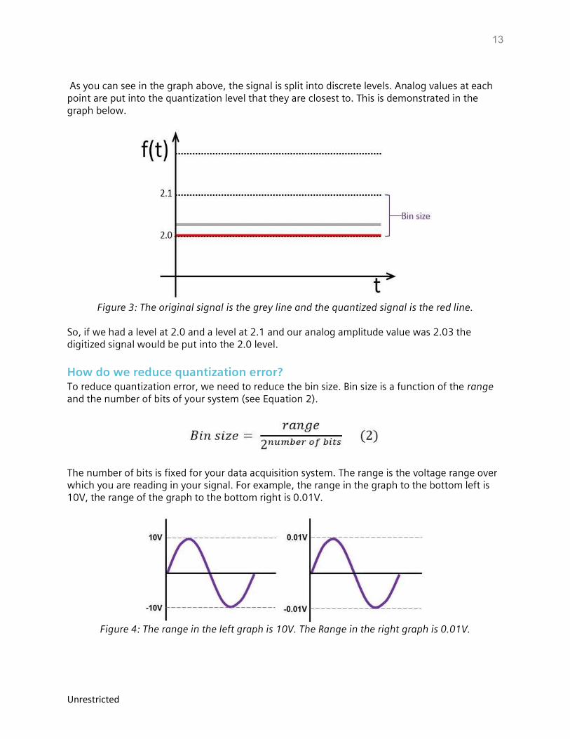
As you can see in the graph above, the signal is split into discrete levels. Analog values at each point are put into the quantization level that they are closest to. This is demonstrated in the graph below.

Figure 3: The original signal is the grey line and the quantized signal is the red line.

So, if we had a level at 2.0 and a level at 2.1 and our analog amplitude value was 2.03 the digitized signal would be put into the 2.0 level.

How do we reduce quantization error? To reduce quantization error, we need to reduce the bin size. Bin size is a function of the range and the number of bits of your system (see Equation 2).

The number of bits is fixed for your data acquisition system. The range is the voltage range over which you are reading in your signal. For example, the range in the graph to the bottom left is 10V, the range of the graph to the bottom right is 0.01V.

Figure 4: The range in the left graph is 10V. The Range in the right graph is 0.01V.

14

Unrestricted

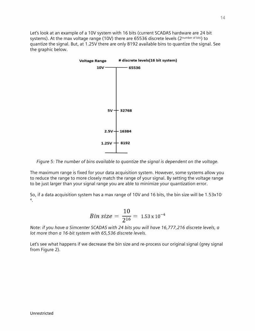
Let’s look at an example of a 10V system with 16 bits (current SCADAS hardware are 24 bit systems). At the max voltage range (10V) there are 65536 discrete levels (2number of bits) to quantize the signal. But, at 1.25V there are only 8192 available bins to quantize the signal. See the graphic below.

Figure 5: The number of bins available to quantize the signal is dependent on the voltage.

The maximum range is fixed for your data acquisition system. However, some systems allow you to reduce the range to more closely match the range of your signal. By setting the voltage range to be just larger than your signal range you are able to minimize your quantization error. So, if a data acquisition system has a max range of 10V and 16 bits, the bin size will be 1.53x10-

4.

Note: if you have a Simcenter SCADAS with 24 bits you will have 16,777,216 discrete levels, a lot more than a 16-bit system with 65,536 discrete levels. Let’s see what happens if we decrease the bin size and re-process our original signal (grey signal from Figure 2).

15

Unrestricted

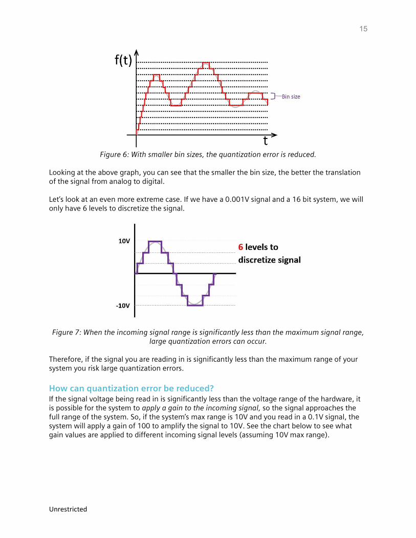
Figure 6: With smaller bin sizes, the quantization error is reduced.

Looking at the above graph, you can see that the smaller the bin size, the better the translation of the signal from analog to digital. Let’s look at an even more extreme case. If we have a 0.001V signal and a 16 bit system, we will only have 6 levels to discretize the signal.

Figure 7: When the incoming signal range is significantly less than the maximum signal range, large quantization errors can occur.

Therefore, if the signal you are reading in is significantly less than the maximum range of your system you risk large quantization errors.

How can quantization error be reduced? If the signal voltage being read in is significantly less than the voltage range of the hardware, it is possible for the system to apply a gain to the incoming signal, so the signal approaches the full range of the system. So, if the system’s max range is 10V and you read in a 0.1V signal, the system will apply a gain of 100 to amplify the signal to 10V. See the chart below to see what gain values are applied to different incoming signal levels (assuming 10V max range).

16

Unrestricted

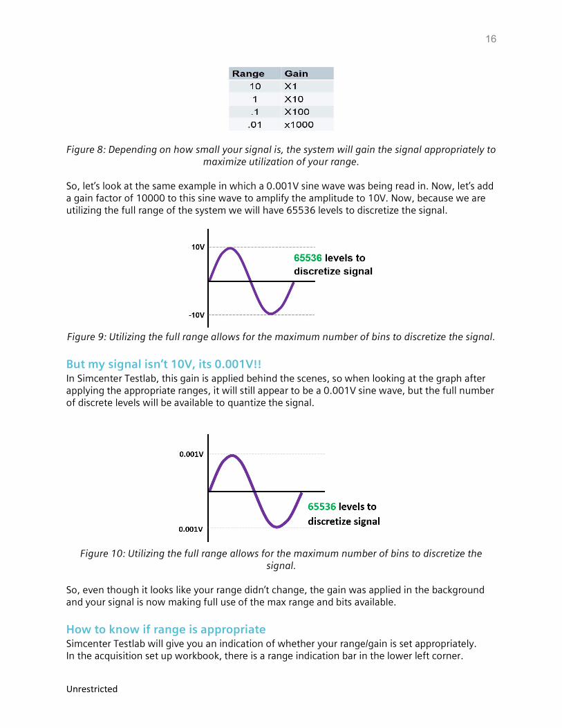
Figure 8: Depending on how small your signal is, the system will gain the signal appropriately to maximize utilization of your range.

So, let’s look at the same example in which a 0.001V sine wave was being read in. Now, let’s add a gain factor of 10000 to this sine wave to amplify the amplitude to 10V. Now, because we are utilizing the full range of the system we will have 65536 levels to discretize the signal.

Figure 9: Utilizing the full range allows for the maximum number of bins to discretize the signal.

But my signal isn’t 10V, its 0.001V!! In Simcenter Testlab, this gain is applied behind the scenes, so when looking at the graph after applying the appropriate ranges, it will still appear to be a 0.001V sine wave, but the full number of discrete levels will be available to quantize the signal.

Figure 10: Utilizing the full range allows for the maximum number of bins to discretize the

signal. So, even though it looks like your range didn’t change, the gain was applied in the background and your signal is now making full use of the max range and bits available.

How to know if range is appropriate Simcenter Testlab will give you an indication of whether your range/gain is set appropriately. In the acquisition set up workbook, there is a range indication bar in the lower left corner.

17

Unrestricted

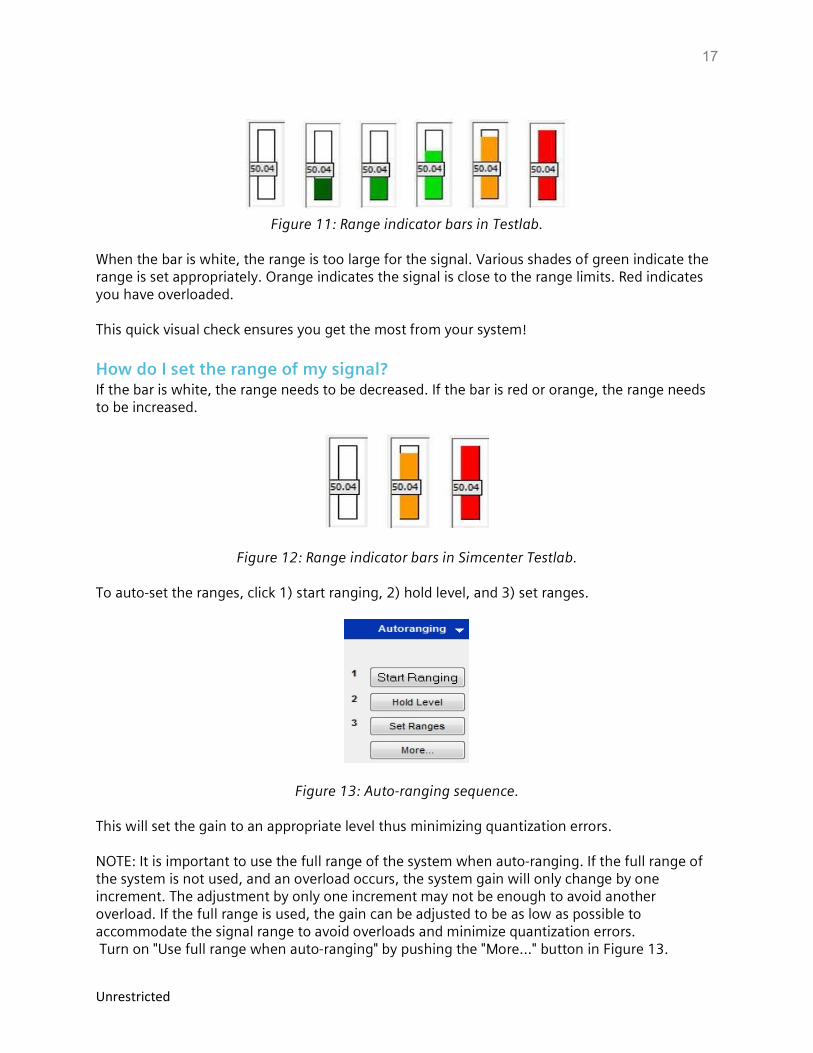
Figure 11: Range indicator bars in Testlab.

When the bar is white, the range is too large for the signal. Various shades of green indicate the range is set appropriately. Orange indicates the signal is close to the range limits. Red indicates you have overloaded. This quick visual check ensures you get the most from your system!

How do I set the range of my signal? If the bar is white, the range needs to be decreased. If the bar is red or orange, the range needs to be increased.

Figure 12: Range indicator bars in Simcenter Testlab. To auto-set the ranges, click 1) start ranging, 2) hold level, and 3) set ranges.

Figure 13: Auto-ranging sequence. This will set the gain to an appropriate level thus minimizing quantization errors. NOTE: It is important to use the full range of the system when auto-ranging. If the full range of the system is not used, and an overload occurs, the system gain will only change by one increment. The adjustment by only one increment may not be enough to avoid another overload. If the full range is used, the gain can be adjusted to be as low as possible to accommodate the signal range to avoid overloads and minimize quantization errors. Turn on "Use full range when auto-ranging" by pushing the "More..." button in Figure 13.

18

Unrestricted

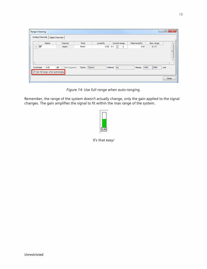
Figure 14: Use full range when auto-ranging.

Remember, the range of the system doesn’t actually change, only the gain applied to the signal changes. The gain amplifies the signal to fit within the max range of the system.

It’s that easy!

19

Unrestricted

Aliasing When converting signals from their true analog form into digital form, frequency errors can be induced due to “aliasing”.

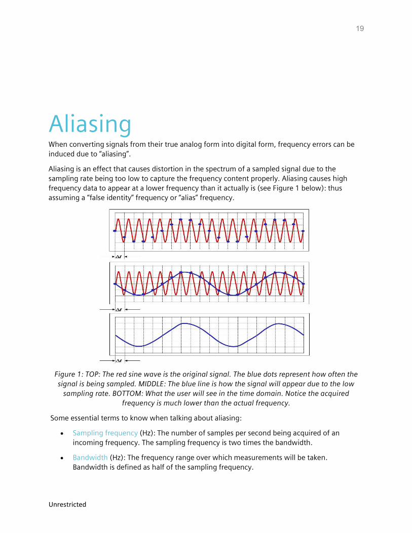
Aliasing is an effect that causes distortion in the spectrum of a sampled signal due to the sampling rate being too low to capture the frequency content properly. Aliasing causes high frequency data to appear at a lower frequency than it actually is (see Figure 1 below): thus assuming a “false identity” frequency or “alias” frequency.

Figure 1: TOP: The red sine wave is the original signal. The blue dots represent how often the signal is being sampled. MIDDLE: The blue line is how the signal will appear due to the low

sampling rate. BOTTOM: What the user will see in the time domain. Notice the acquired frequency is much lower than the actual frequency.

Some essential terms to know when talking about aliasing:

Sampling frequency (Hz): The number of samples per second being acquired of an incoming frequency. The sampling frequency is two times the bandwidth.

Bandwidth (Hz): The frequency range over which measurements will be taken. Bandwidth is defined as half of the sampling frequency.

20

Unrestricted

Span (Hz): The frequency range over which measurements will be taken and not be affected by the anti-aliasing low-pass filters (i.e. the alias-free region of the bandwidth). The span is 80% of the bandwidth.

Nyquist rate (Hz): Minimum frequency at which a signal can be sampled without introducing frequency errors. The Nyquist rate is twice the highest frequency of interest in the sample.

To properly sample all the desired frequency content of an incoming signal, and thereby avoid aliasing, one must sample at (or above) the Nyquist rate. In data acquisition, the sampling frequency is twice as high as the specified bandwidth. So, all frequency content below the specified bandwidth will be sampled at a rate sufficient to accurately capture the frequency content. However, if the incoming signal contains frequency content above the specified bandwidth, the sampling frequency (2x bandwidth) will violate the Nyquist theorem for this higher frequency content.

Figure 2: fs represents the sampling frequency, fsine represents the frequency of the sine wave. a) When sampling at the same frequency as the incoming signal, the observed frequency is 0Hz. b) When sampling at twice the frequency of the sine wave, the observed frequency is fsine, the

true frequency of the sine wave.

When the Nyquist theorem is violated, spectral content above the bandwidth is mirrored about the bandwidth frequency. This means that frequency content X Hz above the bandwidth will then appear X Hz below the bandwidth. Watch the video at the top of this article to see mirroring in action.

Thus, higher frequency content appears to be at a lower frequency, or an “alias” frequency.

21

Unrestricted

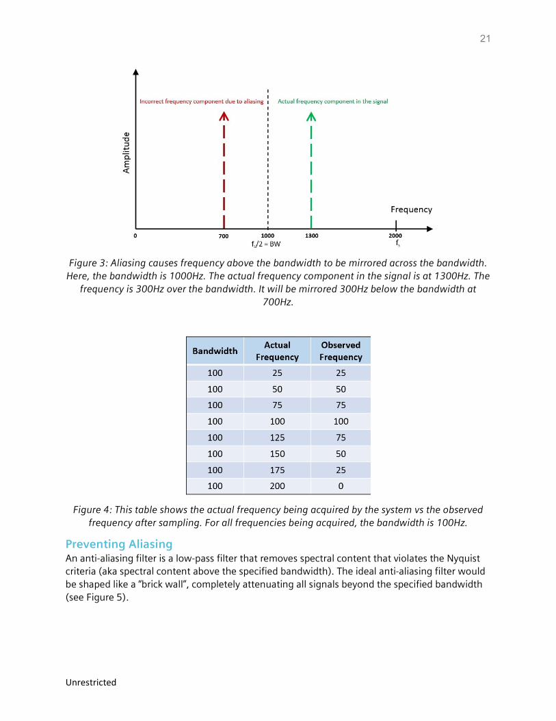
Figure 3: Aliasing causes frequency above the bandwidth to be mirrored across the bandwidth. Here, the bandwidth is 1000Hz. The actual frequency component in the signal is at 1300Hz. The

frequency is 300Hz over the bandwidth. It will be mirrored 300Hz below the bandwidth at 700Hz.

Figure 4: This table shows the actual frequency being acquired by the system vs the observed frequency after sampling. For all frequencies being acquired, the bandwidth is 100Hz.

Preventing Aliasing An anti-aliasing filter is a low-pass filter that removes spectral content that violates the Nyquist criteria (aka spectral content above the specified bandwidth). The ideal anti-aliasing filter would be shaped like a “brick wall”, completely attenuating all signals beyond the specified bandwidth (see Figure 5).

22

Unrestricted

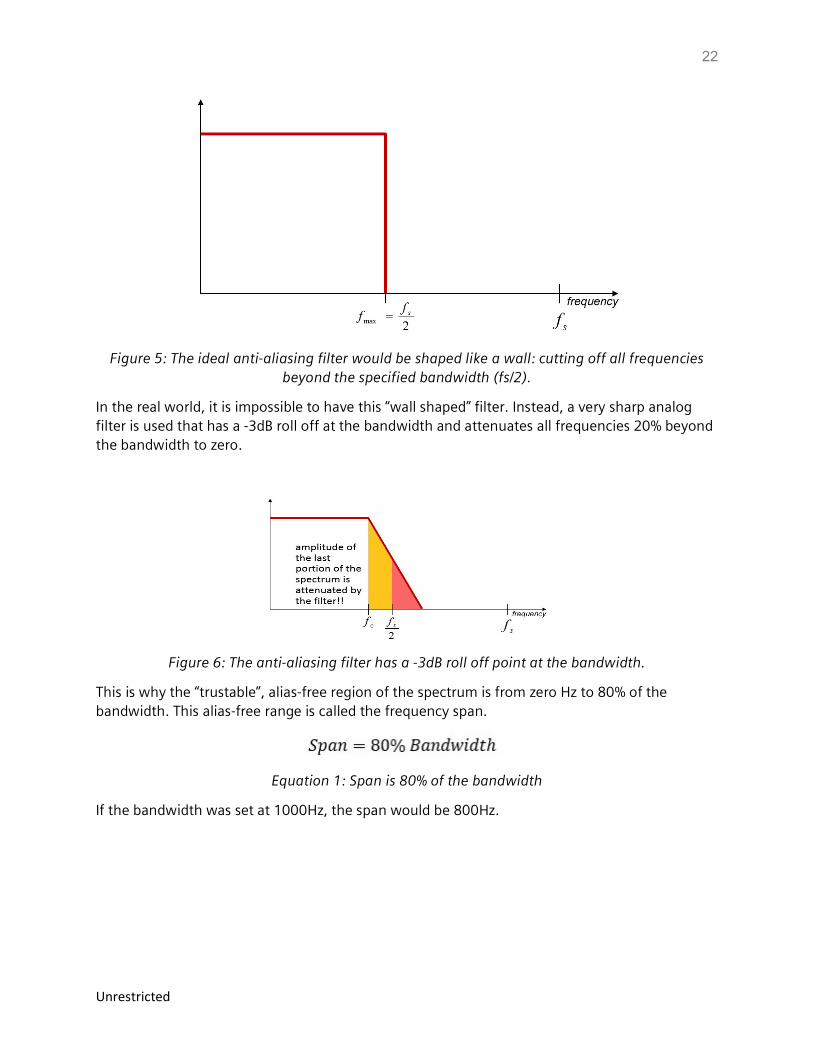
Figure 5: The ideal anti-aliasing filter would be shaped like a wall: cutting off all frequencies beyond the specified bandwidth (fs/2).

In the real world, it is impossible to have this “wall shaped” filter. Instead, a very sharp analog filter is used that has a -3dB roll off at the bandwidth and attenuates all frequencies 20% beyond the bandwidth to zero.

Figure 6: The anti-aliasing filter has a -3dB roll off point at the bandwidth.

This is why the “trustable”, alias-free region of the spectrum is from zero Hz to 80% of the bandwidth. This alias-free range is called the frequency span.

Equation 1: Span is 80% of the bandwidth

If the bandwidth was set at 1000Hz, the span would be 800Hz.

23

Unrestricted

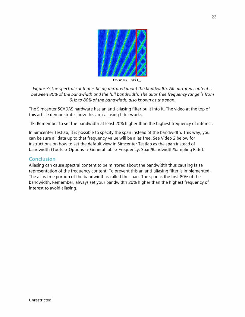
Figure 7: The spectral content is being mirrored about the bandwidth. All mirrored content is between 80% of the bandwidth and the full bandwidth. The alias free frequency range is from

0Hz to 80% of the bandwidth, also known as the span.

The Simcenter SCADAS hardware has an anti-aliasing filter built into it. The video at the top of this article demonstrates how this anti-aliasing filter works.

TIP: Remember to set the bandwidth at least 20% higher than the highest frequency of interest.

In Simcenter Testlab, it is possible to specify the span instead of the bandwidth. This way, you can be sure all data up to that frequency value will be alias free. See Video 2 below for instructions on how to set the default view in Simcenter Testlab as the span instead of bandwidth (Tools -> Options -> General tab -> Frequency: Span/Bandwidth/Sampling Rate).

Conclusion Aliasing can cause spectral content to be mirrored about the bandwidth thus causing false representation of the frequency content. To prevent this an anti-aliasing filter is implemented. The alias-free portion of the bandwidth is called the span. The span is the first 80% of the bandwidth. Remember, always set your bandwidth 20% higher than the highest frequency of interest to avoid aliasing.

24

Unrestricted

Overloads

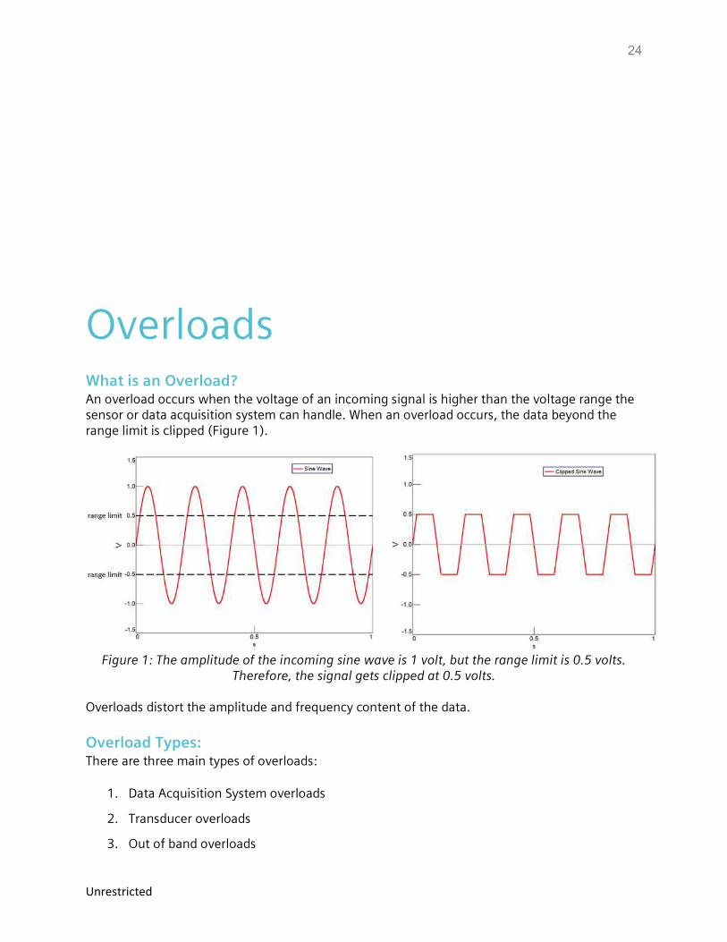
What is an Overload? An overload occurs when the voltage of an incoming signal is higher than the voltage range the sensor or data acquisition system can handle. When an overload occurs, the data beyond the range limit is clipped (Figure 1).

Figure 1: The amplitude of the incoming sine wave is 1 volt, but the range limit is 0.5 volts. Therefore, the signal gets clipped at 0.5 volts.

Overloads distort the amplitude and frequency content of the data.

Overload Types: There are three main types of overloads:

1. Data Acquisition System overloads

2. Transducer overloads

3. Out of band overloads

25

Unrestricted

Data Acquisition System Overloads This type of overload occurs when the range of the data acquisition system is lower than the range of the incoming signal. The incoming signal is clipped as shown in Figure 1 above. Usually when this occurs, a red light appears on the acquisition system and an overload flag is set.

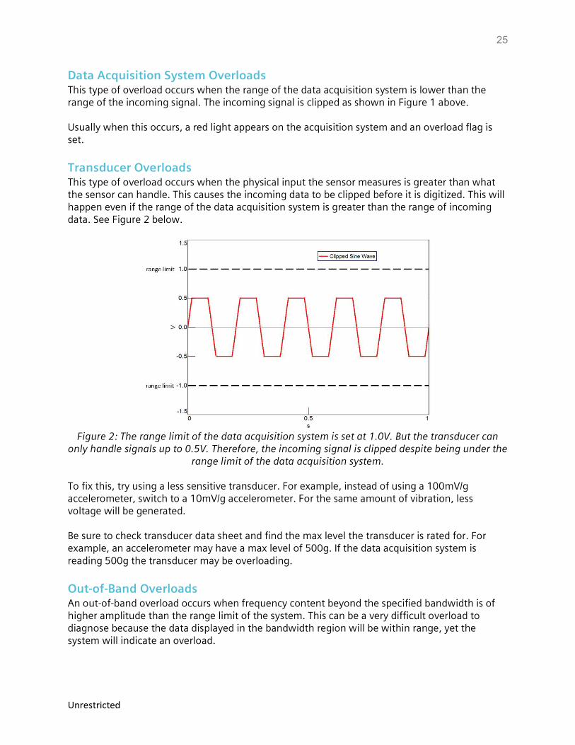
Transducer Overloads This type of overload occurs when the physical input the sensor measures is greater than what the sensor can handle. This causes the incoming data to be clipped before it is digitized. This will happen even if the range of the data acquisition system is greater than the range of incoming data. See Figure 2 below.

Figure 2: The range limit of the data acquisition system is set at 1.0V. But the transducer can

only handle signals up to 0.5V. Therefore, the incoming signal is clipped despite being under the range limit of the data acquisition system.

To fix this, try using a less sensitive transducer. For example, instead of using a 100mV/g accelerometer, switch to a 10mV/g accelerometer. For the same amount of vibration, less voltage will be generated. Be sure to check transducer data sheet and find the max level the transducer is rated for. For example, an accelerometer may have a max level of 500g. If the data acquisition system is reading 500g the transducer may be overloading.

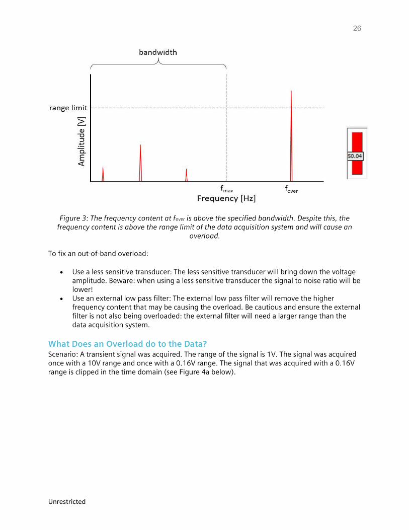
Out-of-Band Overloads An out-of-band overload occurs when frequency content beyond the specified bandwidth is of higher amplitude than the range limit of the system. This can be a very difficult overload to diagnose because the data displayed in the bandwidth region will be within range, yet the system will indicate an overload.

26

Unrestricted

Figure 3: The frequency content at fover is above the specified bandwidth. Despite this, the frequency content is above the range limit of the data acquisition system and will cause an

overload. To fix an out-of-band overload:

Use a less sensitive transducer: The less sensitive transducer will bring down the voltage amplitude. Beware: when using a less sensitive transducer the signal to noise ratio will be lower!

Use an external low pass filter: The external low pass filter will remove the higher frequency content that may be causing the overload. Be cautious and ensure the external filter is not also being overloaded: the external filter will need a larger range than the data acquisition system.

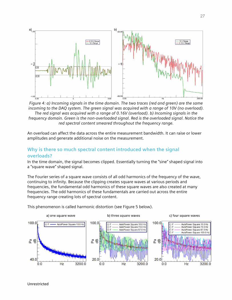
What Does an Overload do to the Data? Scenario: A transient signal was acquired. The range of the signal is 1V. The signal was acquired once with a 10V range and once with a 0.16V range. The signal that was acquired with a 0.16V range is clipped in the time domain (see Figure 4a below).

27

Unrestricted

Figure 4: a) Incoming signals in the time domain. The two traces (red and green) are the same incoming to the DAQ system. The green signal was acquired with a range of 10V (no overload).

The red signal was acquired with a range of 0.16V (overload). b) Incoming signals in the frequency domain. Green is the non-overloaded signal. Red is the overloaded signal. Notice the

red spectral content smeared throughout the frequency range. An overload can affect the data across the entire measurement bandwidth. It can raise or lower amplitudes and generate additional noise on the measurement.

Why is there so much spectral content introduced when the signal overloads? In the time domain, the signal becomes clipped. Essentially turning the “sine” shaped signal into a “square wave” shaped signal. The Fourier series of a square wave consists of all odd harmonics of the frequency of the wave, continuing to infinity. Because the clipping creates square waves at various periods and frequencies, the fundamental odd harmonics of these square waves are also created at many frequencies. The odd harmonics of these fundamentals are carried out across the entire frequency range creating lots of spectral content. This phenomenon is called harmonic distortion (see Figure 5 below).

28

Unrestricted

Figure 5: a) The spectrum of one square wave. b) The spectrum of three square waves at different frequencies. c) The spectrum of four square waves at different frequencies.

You can see that even with just three or four square waves at different frequencies, harmonic distortion effects the spectrum greatly. Overloads greatly affect the resultant spectrum! WARNING: Even if the overload is out of range you will still get harmonic distortion across your entire frequency range. The overload will still affect your data even if it’s out of band!

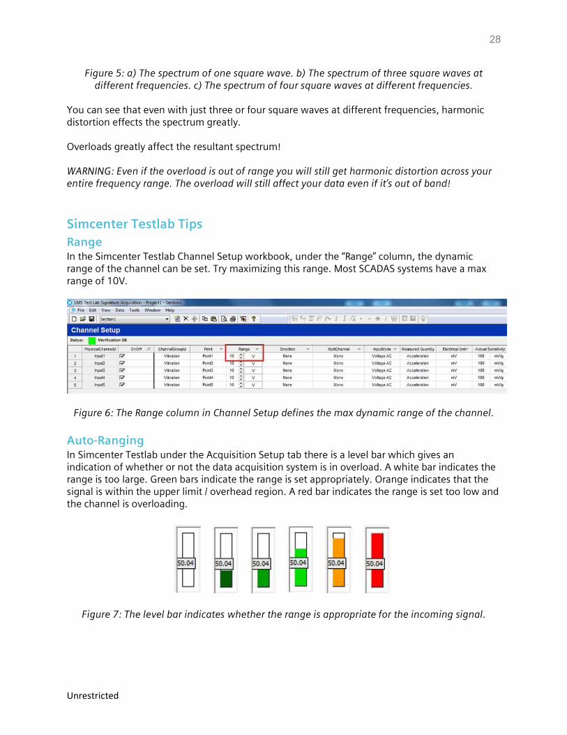
Simcenter Testlab Tips Range In the Simcenter Testlab Channel Setup workbook, under the “Range” column, the dynamic range of the channel can be set. Try maximizing this range. Most SCADAS systems have a max range of 10V.

Figure 6: The Range column in Channel Setup defines the max dynamic range of the channel.

Auto-Ranging In Simcenter Testlab under the Acquisition Setup tab there is a level bar which gives an indication of whether or not the data acquisition system is in overload. A white bar indicates the range is too large. Green bars indicate the range is set appropriately. Orange indicates that the signal is within the upper limit / overhead region. A red bar indicates the range is set too low and the channel is overloading.

Figure 7: The level bar indicates whether the range is appropriate for the incoming signal.

29

Unrestricted

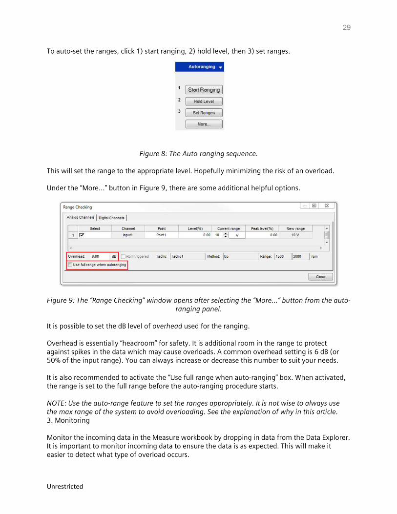
To auto-set the ranges, click 1) start ranging, 2) hold level, then 3) set ranges.

Figure 8: The Auto-ranging sequence. This will set the range to the appropriate level. Hopefully minimizing the risk of an overload. Under the “More…” button in Figure 9, there are some additional helpful options.

Figure 9: The “Range Checking” window opens after selecting the “More…” button from the auto-ranging panel.

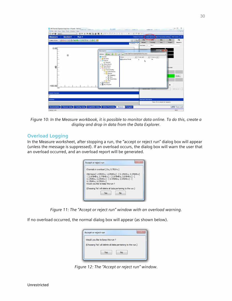
It is possible to set the dB level of overhead used for the ranging. Overhead is essentially “headroom” for safety. It is additional room in the range to protect against spikes in the data which may cause overloads. A common overhead setting is 6 dB (or 50% of the input range). You can always increase or decrease this number to suit your needs. It is also recommended to activate the “Use full range when auto-ranging” box. When activated, the range is set to the full range before the auto-ranging procedure starts. NOTE: Use the auto-range feature to set the ranges appropriately. It is not wise to always use the max range of the system to avoid overloading. See the explanation of why in this article. 3. Monitoring Monitor the incoming data in the Measure workbook by dropping in data from the Data Explorer. It is important to monitor incoming data to ensure the data is as expected. This will make it easier to detect what type of overload occurs.

30

Unrestricted

Figure 10: In the Measure workbook, it is possible to monitor data online. To do this, create a display and drop in data from the Data Explorer.

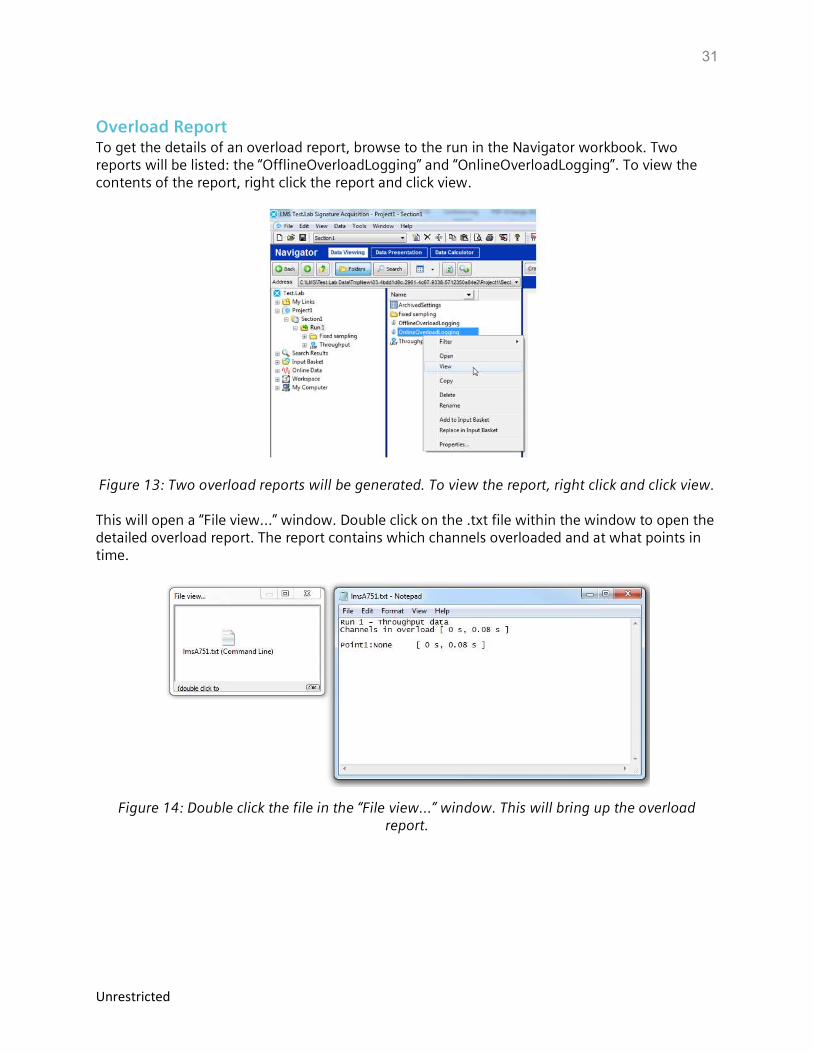
Overload Logging In the Measure worksheet, after stopping a run, the “accept or reject run” dialog box will appear (unless the message is suppressed). If an overload occurs, the dialog box will warn the user that an overload occurred, and an overload report will be generated.

Figure 11: The “Accept or reject run” window with an overload warning. If no overload occurred, the normal dialog box will appear (as shown below).

Figure 12: The “Accept or reject run” window.

31

Unrestricted

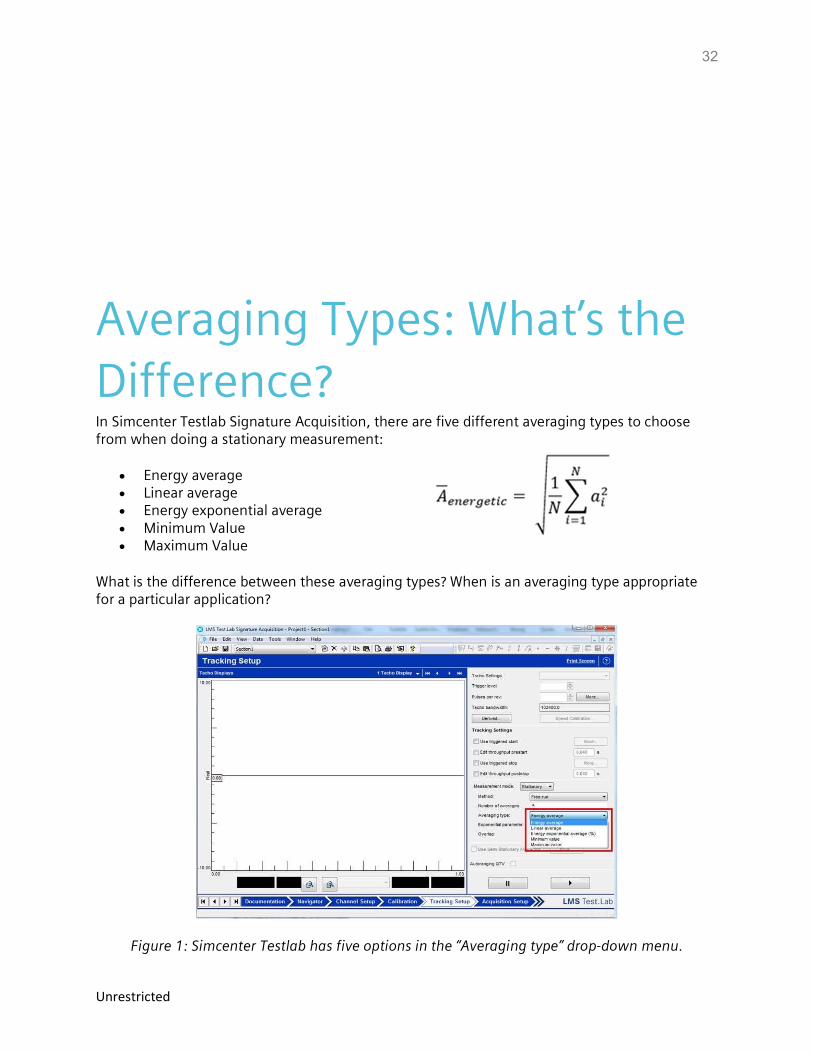
Overload Report To get the details of an overload report, browse to the run in the Navigator workbook. Two reports will be listed: the “OfflineOverloadLogging” and “OnlineOverloadLogging”. To view the contents of the report, right click the report and click view.

Figure 13: Two overload reports will be generated. To view the report, right click and click view. This will open a “File view…” window. Double click on the .txt file within the window to open the detailed overload report. The report contains which channels overloaded and at what points in time.

Figure 14: Double click the file in the “File view…” window. This will bring up the overload report.

32

Unrestricted

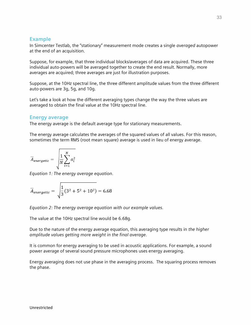
Averaging Types: What’s the Difference? In Simcenter Testlab Signature Acquisition, there are five different averaging types to choose from when doing a stationary measurement:

Energy average Linear average Energy exponential average Minimum Value Maximum Value

What is the difference between these averaging types? When is an averaging type appropriate for a particular application?

Figure 1: Simcenter Testlab has five options in the “Averaging type” drop-down menu.

33

Unrestricted

Example In Simcenter Testlab, the “stationary” measurement mode creates a single averaged autopower at the end of an acquisition. Suppose, for example, that three individual blocks/averages of data are acquired. These three individual auto-powers will be averaged together to create the end result. Normally, more averages are acquired; three averages are just for illustration purposes. Suppose, at the 10Hz spectral line, the three different amplitude values from the three different auto-powers are 3g, 5g, and 10g. Let’s take a look at how the different averaging types change the way the three values are averaged to obtain the final value at the 10Hz spectral line.

Energy average The energy average is the default average type for stationary measurements. The energy average calculates the averages of the squared values of all values. For this reason, sometimes the term RMS (root mean square) average is used in lieu of energy average.

Equation 1: The energy average equation.

Equation 2: The energy average equation with our example values. The value at the 10Hz spectral line would be 6.68g. Due to the nature of the energy average equation, this averaging type results in the higher amplitude values getting more weight in the final average. It is common for energy averaging to be used in acoustic applications. For example, a sound power average of several sound pressure microphones uses energy averaging. Energy averaging does not use phase in the averaging process. The squaring process removes the phase.

34

Unrestricted

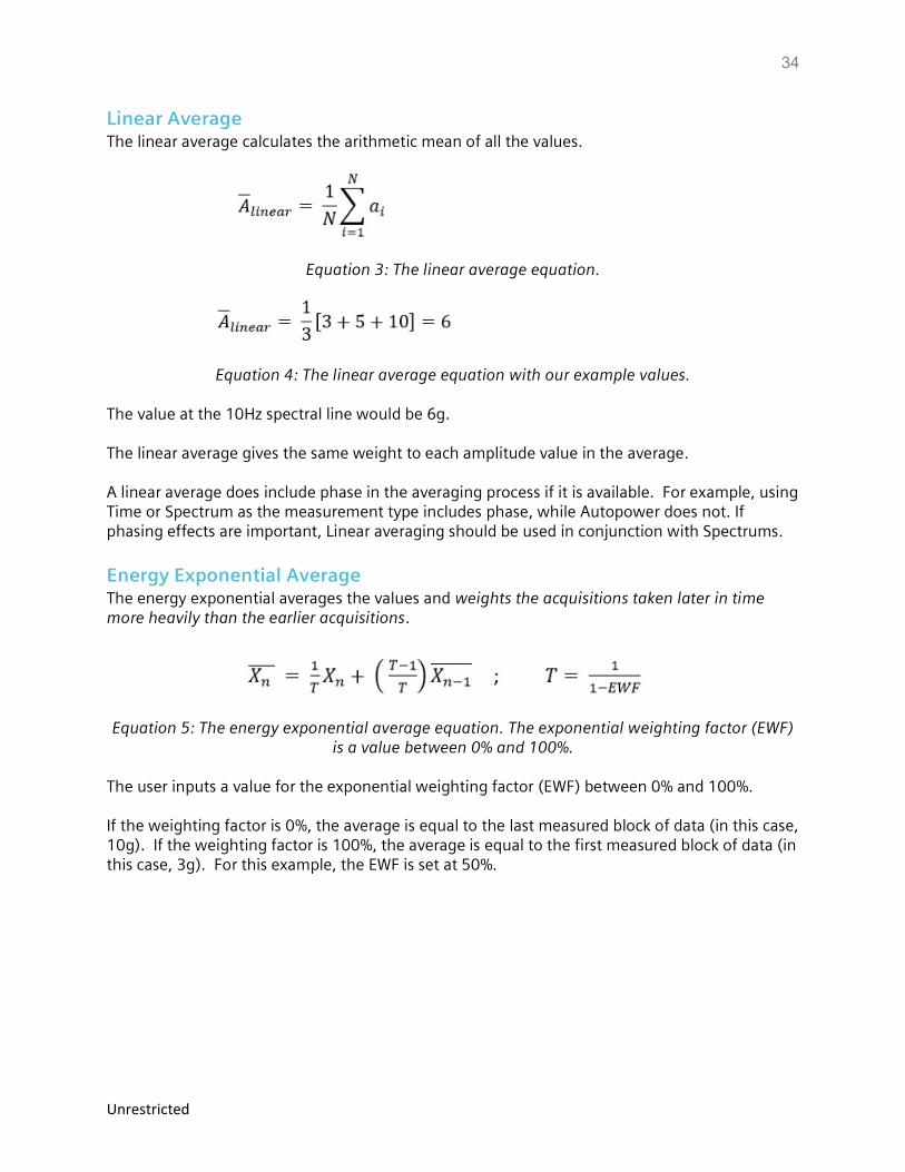
Linear Average The linear average calculates the arithmetic mean of all the values.

Equation 3: The linear average equation.

Equation 4: The linear average equation with our example values. The value at the 10Hz spectral line would be 6g. The linear average gives the same weight to each amplitude value in the average. A linear average does include phase in the averaging process if it is available. For example, using Time or Spectrum as the measurement type includes phase, while Autopower does not. If phasing effects are important, Linear averaging should be used in conjunction with Spectrums.

Energy Exponential Average The energy exponential averages the values and weights the acquisitions taken later in time more heavily than the earlier acquisitions.

Equation 5: The energy exponential average equation. The exponential weighting factor (EWF) is a value between 0% and 100%.

The user inputs a value for the exponential weighting factor (EWF) between 0% and 100%. If the weighting factor is 0%, the average is equal to the last measured block of data (in this case, 10g). If the weighting factor is 100%, the average is equal to the first measured block of data (in this case, 3g). For this example, the EWF is set at 50%.

35

Unrestricted

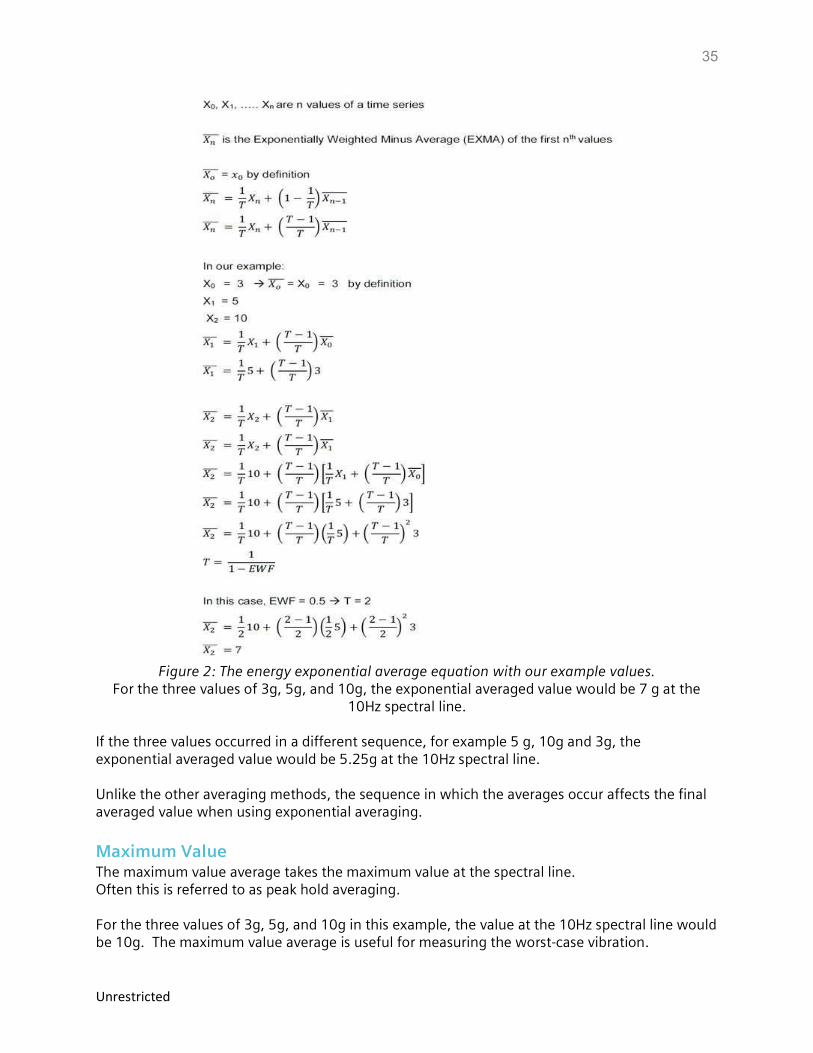
Figure 2: The energy exponential average equation with our example values.

For the three values of 3g, 5g, and 10g, the exponential averaged value would be 7 g at the 10Hz spectral line.

If the three values occurred in a different sequence, for example 5 g, 10g and 3g, the exponential averaged value would be 5.25g at the 10Hz spectral line. Unlike the other averaging methods, the sequence in which the averages occur affects the final averaged value when using exponential averaging.

Maximum Value The maximum value average takes the maximum value at the spectral line. Often this is referred to as peak hold averaging. For the three values of 3g, 5g, and 10g in this example, the value at the 10Hz spectral line would be 10g. The maximum value average is useful for measuring the worst-case vibration.

36

Unrestricted

Minimum Value The minimum value average takes the minimum value at the spectral line. For the three values of 3g, 5g, and 10g in this example, the value at the 10Hz spectral line would be 3g. The minimum value may be used in conjunction with the max value averaging type to get an envelope or range of values for the spectrum.

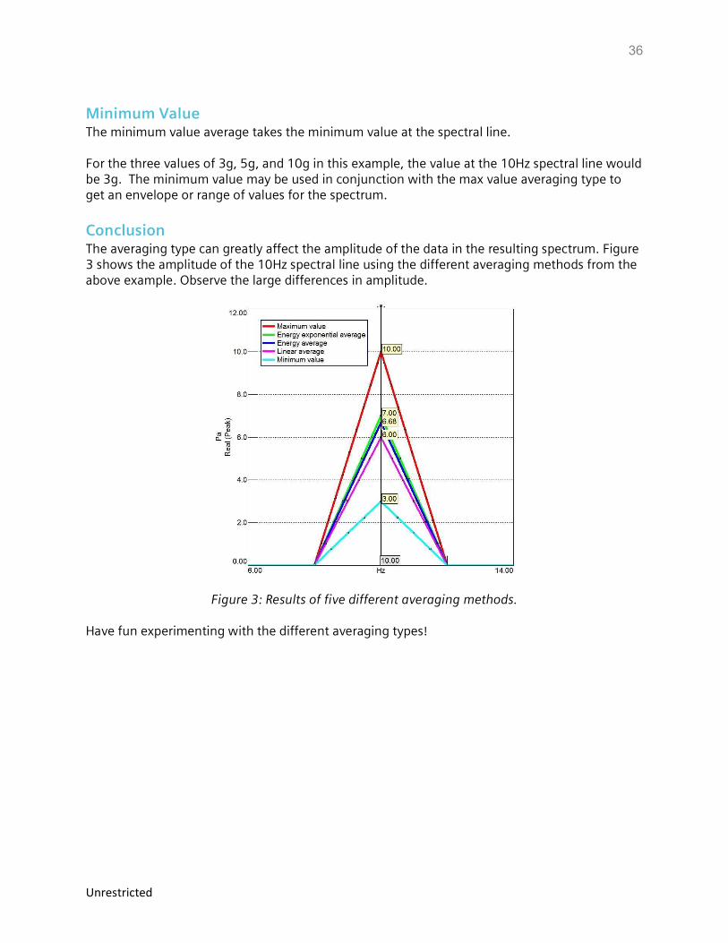
Conclusion The averaging type can greatly affect the amplitude of the data in the resulting spectrum. Figure 3 shows the amplitude of the 10Hz spectral line using the different averaging methods from the above example. Observe the large differences in amplitude.

Figure 3: Results of five different averaging methods. Have fun experimenting with the different averaging types!

37

Unrestricted

Spectrum Versus Autopower

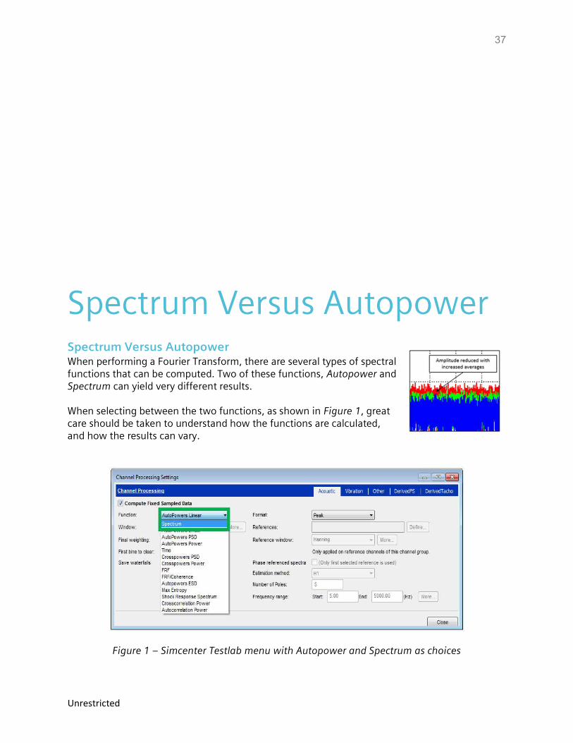
Spectrum Versus Autopower When performing a Fourier Transform, there are several types of spectral functions that can be computed. Two of these functions, Autopower and Spectrum can yield very different results. When selecting between the two functions, as shown in Figure 1, great care should be taken to understand how the functions are calculated, and how the results can vary.

Figure 1 – Simcenter Testlab menu with Autopower and Spectrum as choices

38

Unrestricted

Results can be affected by amplitude, phase, and averaging. This article explains the background and differences between the two functions and when to use them.

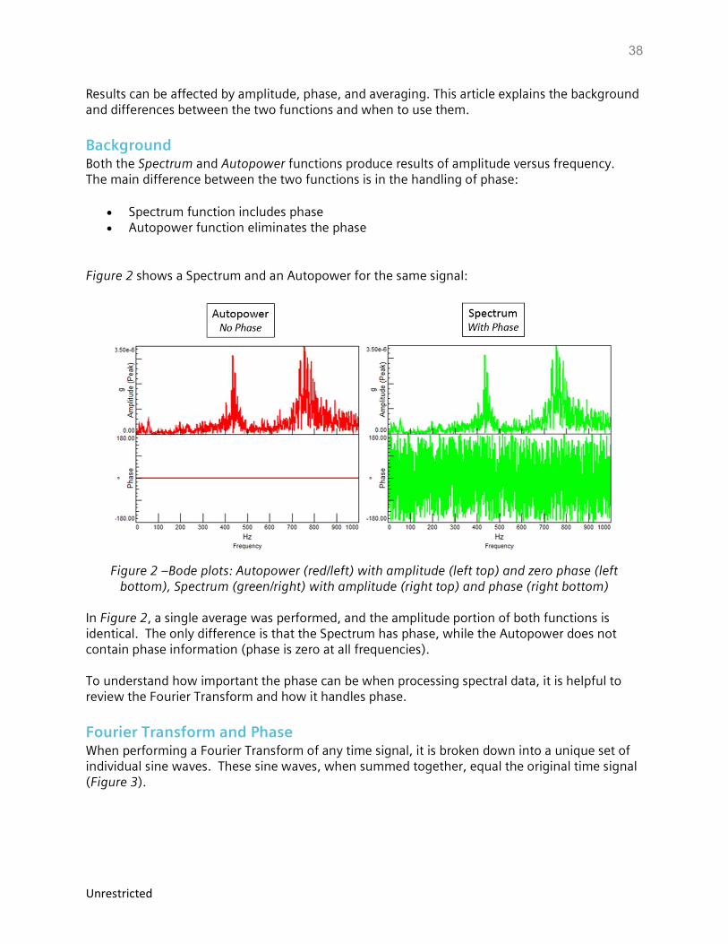
Background Both the Spectrum and Autopower functions produce results of amplitude versus frequency. The main difference between the two functions is in the handling of phase:

Spectrum function includes phase Autopower function eliminates the phase

Figure 2 shows a Spectrum and an Autopower for the same signal:

Figure 2 –Bode plots: Autopower (red/left) with amplitude (left top) and zero phase (left

bottom), Spectrum (green/right) with amplitude (right top) and phase (right bottom) In Figure 2, a single average was performed, and the amplitude portion of both functions is identical. The only difference is that the Spectrum has phase, while the Autopower does not contain phase information (phase is zero at all frequencies). To understand how important the phase can be when processing spectral data, it is helpful to review the Fourier Transform and how it handles phase.

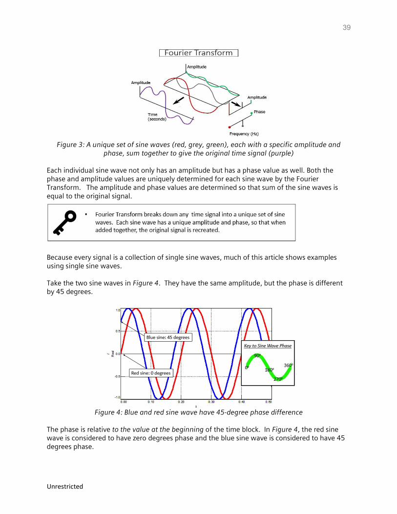
Fourier Transform and Phase When performing a Fourier Transform of any time signal, it is broken down into a unique set of individual sine waves. These sine waves, when summed together, equal the original time signal (Figure 3).

39

Unrestricted

Figure 3: A unique set of sine waves (red, grey, green), each with a specific amplitude and

phase, sum together to give the original time signal (purple) Each individual sine wave not only has an amplitude but has a phase value as well. Both the phase and amplitude values are uniquely determined for each sine wave by the Fourier Transform. The amplitude and phase values are determined so that sum of the sine waves is equal to the original signal.

Because every signal is a collection of single sine waves, much of this article shows examples using single sine waves. Take the two sine waves in Figure 4. They have the same amplitude, but the phase is different by 45 degrees.

Figure 4: Blue and red sine wave have 45-degree phase difference

The phase is relative to the value at the beginning of the time block. In Figure 4, the red sine wave is considered to have zero degrees phase and the blue sine wave is considered to have 45 degrees phase.

40

Unrestricted

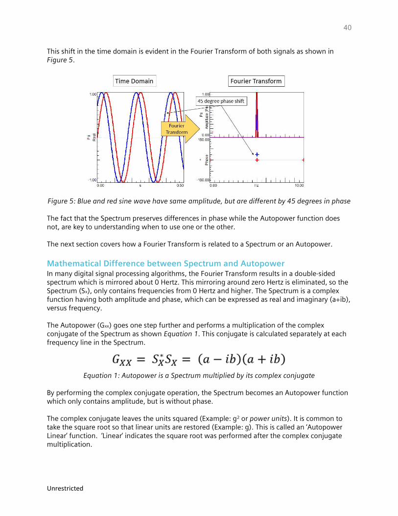
This shift in the time domain is evident in the Fourier Transform of both signals as shown in Figure 5.

Figure 5: Blue and red sine wave have same amplitude, but are different by 45 degrees in phase The fact that the Spectrum preserves differences in phase while the Autopower function does not, are key to understanding when to use one or the other. The next section covers how a Fourier Transform is related to a Spectrum or an Autopower.

Mathematical Difference between Spectrum and Autopower In many digital signal processing algorithms, the Fourier Transform results in a double-sided spectrum which is mirrored about 0 Hertz. This mirroring around zero Hertz is eliminated, so the Spectrum (Sx), only contains frequencies from 0 Hertz and higher. The Spectrum is a complex function having both amplitude and phase, which can be expressed as real and imaginary (a+ib), versus frequency. The Autopower (Gxx) goes one step further and performs a multiplication of the complex conjugate of the Spectrum as shown Equation 1. This conjugate is calculated separately at each frequency line in the Spectrum.

Equation 1: Autopower is a Spectrum multiplied by its complex conjugate

By performing the complex conjugate operation, the Spectrum becomes an Autopower function which only contains amplitude, but is without phase. The complex conjugate leaves the units squared (Example: g2 or power units). It is common to take the square root so that linear units are restored (Example: g). This is called an ‘Autopower Linear’ function. ‘Linear’ indicates the square root was performed after the complex conjugate multiplication.

41

Unrestricted

Selecting either Autopower or Spectrum is also an important consideration if averaging of multiple functions or samples will be performed, which is discussed in the next section.

Averaging Considerations In Figure 6, the time domain and frequency domain of two different sine waves are shown. The two sine waves are 180 degrees out of phase.

Figure 6 – Left: Time domain of two sine waves with 180-degree phase difference. Right:

Spectrum of the two sine waves shows the same 180-degree phase difference. If the two sine waves are averaged, the result would be zero. Whether performing the average in the time domain or in the frequency domain, the average would be zero. Using a Autopower, however, it can be made so the average will not be zero in the frequency domain. In Figure 7, the Autopower of both sine waves is shown. Notice that the phase of the Autopower of both sine waves is zero, and identical. The phase of the Autopower in the frequency domain is the same, even though the two sine waves are clearly out of phase in the time domain.

Figure 7: Autopower function average will be correct, due to elimination of phase.

Time domain average would still be zero.

42

Unrestricted

In this case, while the average in the time domain would be zero, the average of the Autopower functions in the frequency domain would be correct. The average would not be zero in the frequency domain, thanks to the Autopower function!

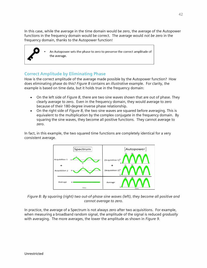
Correct Amplitude by Eliminating Phase How is the correct amplitude of the average made possible by the Autopower function? How does eliminating phase do this? Figure 8 contains an illustrative example. For clarity, the example is based on time data, but it holds true in the frequency domain:

On the left side of Figure 8, there are two sine waves shown that are out of phase. They clearly average to zero. Even in the frequency domain, they would average to zero because of their 180-degree inverse phase relationship.

On the right side of Figure 8, the two sine waves are squared before averaging. This is equivalent to the multiplication by the complex conjugate in the frequency domain. By squaring the sine waves, they become all positive functions. They cannot average to zero.

In fact, in this example, the two squared time functions are completely identical for a very consistent average.

Figure 8: By squaring (right) two out-of-phase sine waves (left), they become all positive and cannot average to zero.

In practice, the average of a Spectrum is not always zero after two acquisitions. For example, when measuring a broadband random signal, the amplitude of the signal is reduced gradually with averaging. The more averages, the lower the amplitude as shown in Figure 9.

43

Unrestricted

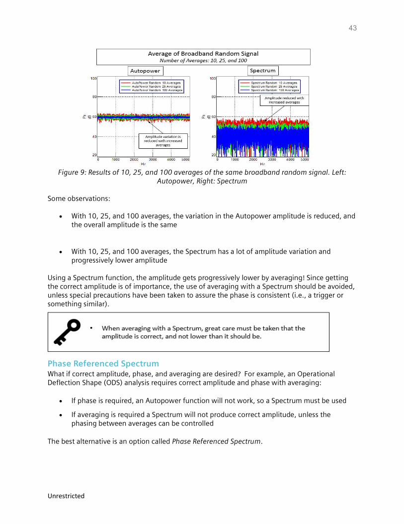
Figure 9: Results of 10, 25, and 100 averages of the same broadband random signal. Left:

Autopower, Right: Spectrum Some observations:

With 10, 25, and 100 averages, the variation in the Autopower amplitude is reduced, and the overall amplitude is the same

With 10, 25, and 100 averages, the Spectrum has a lot of amplitude variation and progressively lower amplitude

Using a Spectrum function, the amplitude gets progressively lower by averaging! Since getting the correct amplitude is of importance, the use of averaging with a Spectrum should be avoided, unless special precautions have been taken to assure the phase is consistent (i.e., a trigger or something similar).

Phase Referenced Spectrum What if correct amplitude, phase, and averaging are desired? For example, an Operational Deflection Shape (ODS) analysis requires correct amplitude and phase with averaging:

If phase is required, an Autopower function will not work, so a Spectrum must be used

If averaging is required a Spectrum will not produce correct amplitude, unless the phasing between averages can be controlled

The best alternative is an option called Phase Referenced Spectrum.

44

Unrestricted

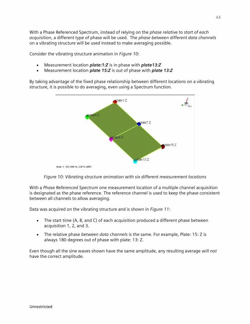
With a Phase Referenced Spectrum, instead of relying on the phase relative to start of each acquisition, a different type of phase will be used. The phase between different data channels on a vibrating structure will be used instead to make averaging possible. Consider the vibrating structure animation in Figure 10:

Measurement location plate:1:Z is in phase with plate13:Z Measurement location plate 15:Z is out of phase with plate 13:Z

By taking advantage of the fixed phase relationship between different locations on a vibrating structure, it is possible to do averaging, even using a Spectrum function.

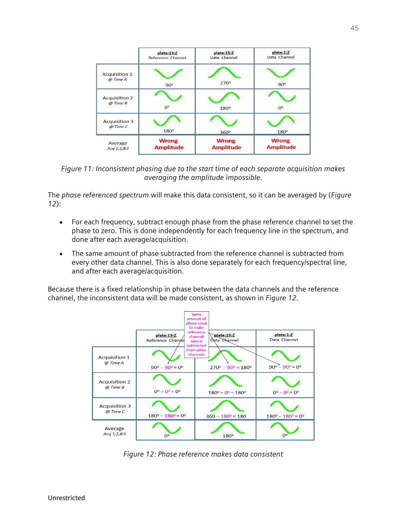
Figure 10: Vibrating structure animation with six different measurement locations With a Phase Referenced Spectrum one measurement location of a multiple channel acquisition is designated as the phase reference. The reference channel is used to keep the phase consistent between all channels to allow averaging. Data was acquired on the vibrating structure and is shown in Figure 11:

The start time (A, B, and C) of each acquisition produced a different phase between acquisition 1, 2, and 3.

The relative phase between data channels is the same. For example, Plate: 15: Z is always 180 degrees out of phase with plate: 13: Z.

Even though all the sine waves shown have the same amplitude, any resulting average will not have the correct amplitude.

45

Unrestricted

Figure 11: Inconsistent phasing due to the start time of each separate acquisition makes averaging the amplitude impossible.

The phase referenced spectrum will make this data consistent, so it can be averaged by (Figure 12):

For each frequency, subtract enough phase from the phase reference channel to set the phase to zero. This is done independently for each frequency line in the spectrum, and done after each average/acquisition.

The same amount of phase subtracted from the reference channel is subtracted from every other data channel. This is also done separately for each frequency/spectral line, and after each average/acquisition.

Because there is a fixed relationship in phase between the data channels and the reference channel, the inconsistent data will be made consistent, as shown in Figure 12.

Figure 12: Phase reference makes data consistent

46

Unrestricted

This allows the averaging to be done properly and results in the correct amplitude value. Of course, at frequencies where there is no relationship between channels, this will not be the case. For example, phase referencing will not work with data channels being acquired on a vehicle if the phase reference channel is on the laboratory floor. The phase reference channel instead should be a data channel on the vehicle that is very active. Will the phase referenced spectrum and an autopower have exactly the same amplitude? Probably not. Any random vibration in the structure that has no fixed phase relationship to other locations will be averaged out. So there can be differences depending on how much the vibration of different locations on the structure are related to each other. Note that this example is shown for one frequency in the time domain for illustrative purposes. The ‘Phase Referenced Spectrum’ will work on all frequencies independently in the spectrum. The amount of phase subtracted is not always 0, 90, or 180 degrees. It can be any

phase amount (33, 48, 56 degrees) that is present in the vibrating structure between different locations.

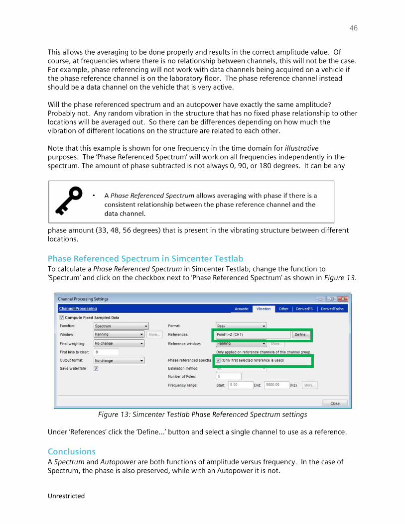
Phase Referenced Spectrum in Simcenter Testlab To calculate a Phase Referenced Spectrum in Simcenter Testlab, change the function to ‘Spectrum’ and click on the checkbox next to ‘Phase Referenced Spectrum’ as shown in Figure 13.

Figure 13: Simcenter Testlab Phase Referenced Spectrum settings

Under ‘References’ click the ‘Define…’ button and select a single channel to use as a reference.

Conclusions A Spectrum and Autopower are both functions of amplitude versus frequency. In the case of Spectrum, the phase is also preserved, while with an Autopower it is not.

47

Unrestricted

Be careful using Spectrum when averaging data. It is easy to get the wrong amplitude. Use Autopower for applications where only amplitude is required. Use a Phase Referenced Spectrum when phasing and averaging are both required.

Enjoy Spectrums and Auto-powers!

48

Unrestricted

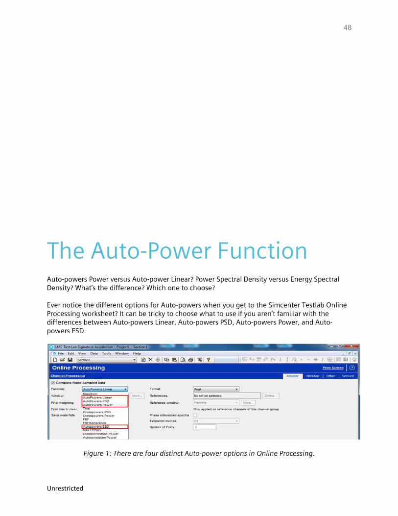
The Auto-Power Function Auto-powers Power versus Auto-power Linear? Power Spectral Density versus Energy Spectral Density? What’s the difference? Which one to choose? Ever notice the different options for Auto-powers when you get to the Simcenter Testlab Online Processing worksheet? It can be tricky to choose what to use if you aren’t familiar with the differences between Auto-powers Linear, Auto-powers PSD, Auto-powers Power, and Auto-powers ESD.

Figure 1: There are four distinct Auto-power options in Online Processing.

49

Unrestricted

Auto-powers Power (Auto-power Spectrum) The Auto-power power (also called Auto-power spectrum) is the squared magnitude of the frequency spectrum.

Equation 1: GXX is the Auto-power spectrum. SX is the frequency spectrum. Sx* is the complex

conjugate of the frequency spectrum. The Auto-power spectrum is created by multiplying a frequency spectrum by its complex conjugate.

This results in the Auto-power spectrum equaling the magnitude of the frequency spectrum squared. There is no phase information (as the Auto-power spectrum is all real, no imaginary component).

Figure 2: Example Auto-power power: The y-axis is the amplitude unit squared. The x-axis is in frequency. There is no phase information.

Consider an average of these two functions: a sine wave and an inverse sine wave. If they are averaged, the result will be zero.

Figure 3: A sine wave and inverse sine wave sum to zero amplitude.

Before averaging, suppose the functions were squared (Figure 4). Would the functions still average to zero? No, they would not!

50

Unrestricted

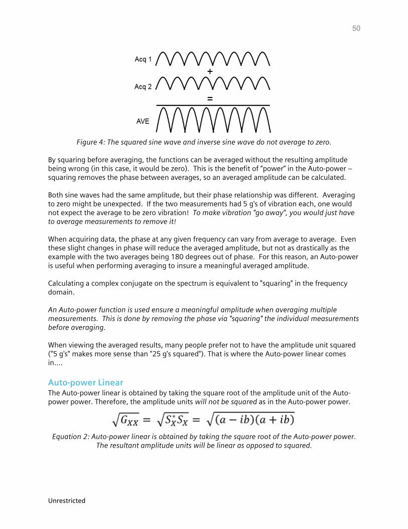
Figure 4: The squared sine wave and inverse sine wave do not average to zero.

By squaring before averaging, the functions can be averaged without the resulting amplitude being wrong (in this case, it would be zero). This is the benefit of “power” in the Auto-power – squaring removes the phase between averages, so an averaged amplitude can be calculated. Both sine waves had the same amplitude, but their phase relationship was different. Averaging to zero might be unexpected. If the two measurements had 5 g's of vibration each, one would not expect the average to be zero vibration! To make vibration "go away", you would just have to average measurements to remove it! When acquiring data, the phase at any given frequency can vary from average to average. Even these slight changes in phase will reduce the averaged amplitude, but not as drastically as the example with the two averages being 180 degrees out of phase. For this reason, an Auto-power is useful when performing averaging to insure a meaningful averaged amplitude. Calculating a complex conjugate on the spectrum is equivalent to "squaring" in the frequency domain. An Auto-power function is used ensure a meaningful amplitude when averaging multiple measurements. This is done by removing the phase via "squaring" the individual measurements before averaging. When viewing the averaged results, many people prefer not to have the amplitude unit squared ("5 g's" makes more sense than "25 g's squared"). That is where the Auto-power linear comes in….

Auto-power Linear The Auto-power linear is obtained by taking the square root of the amplitude unit of the Auto-power power. Therefore, the amplitude units will not be squared as in the Auto-power power.

Equation 2: Auto-power linear is obtained by taking the square root of the Auto-power power.

The resultant amplitude units will be linear as opposed to squared.

51

Unrestricted

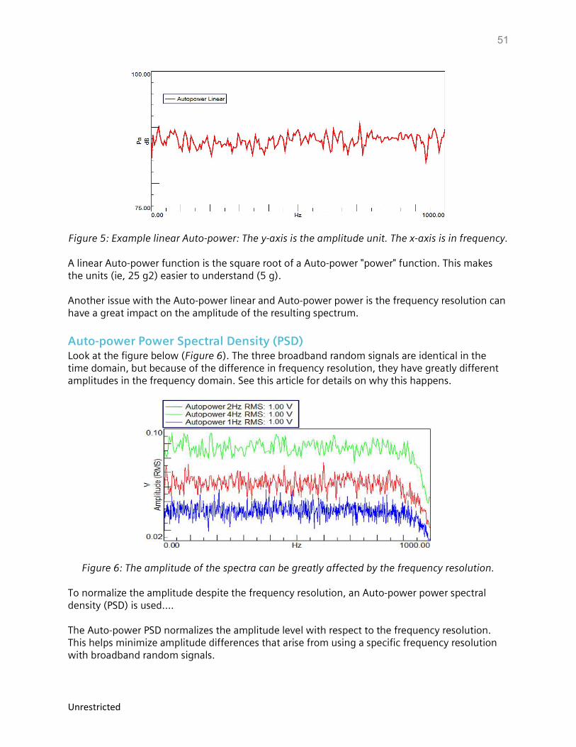
Figure 5: Example linear Auto-power: The y-axis is the amplitude unit. The x-axis is in frequency. A linear Auto-power function is the square root of a Auto-power "power" function. This makes the units (ie, 25 g2) easier to understand (5 g). Another issue with the Auto-power linear and Auto-power power is the frequency resolution can have a great impact on the amplitude of the resulting spectrum.

Auto-power Power Spectral Density (PSD) Look at the figure below (Figure 6). The three broadband random signals are identical in the time domain, but because of the difference in frequency resolution, they have greatly different amplitudes in the frequency domain. See this article for details on why this happens.

Figure 6: The amplitude of the spectra can be greatly affected by the frequency resolution. To normalize the amplitude despite the frequency resolution, an Auto-power power spectral density (PSD) is used…. The Auto-power PSD normalizes the amplitude level with respect to the frequency resolution. This helps minimize amplitude differences that arise from using a specific frequency resolution with broadband random signals.

52

Unrestricted

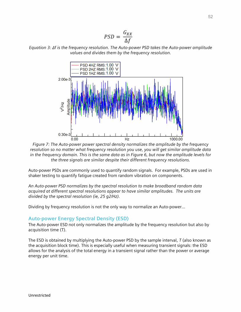
Equation 3: Δf is the frequency resolution. The Auto-power PSD takes the Auto-power amplitude

values and divides them by the frequency resolution.

Figure 7: The Auto-power power spectral density normalizes the amplitude by the frequency

resolution so no matter what frequency resolution you use, you will get similar amplitude data in the frequency domain. This is the same data as in Figure 6, but now the amplitude levels for

the three signals are similar despite their different frequency resolutions. Auto-power PSDs are commonly used to quantify random signals. For example, PSDs are used in shaker testing to quantify fatigue created from random vibration on components. An Auto-power PSD normalizes by the spectral resolution to make broadband random data acquired at different spectral resolutions appear to have similar amplitudes. The units are divided by the spectral resolution (ie, 25 g2/Hz). Dividing by frequency resolution is not the only way to normalize an Auto-power...

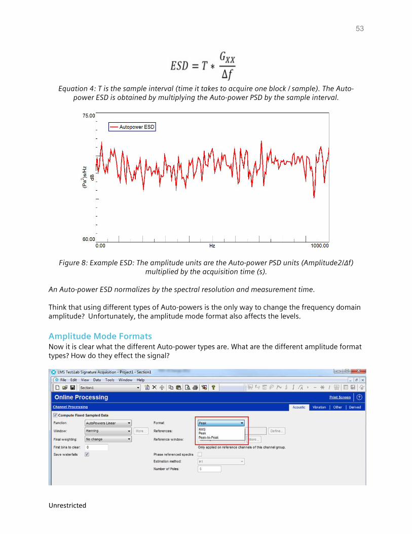
Auto-power Energy Spectral Density (ESD) The Auto-power ESD not only normalizes the amplitude by the frequency resolution but also by acquisition time (T). The ESD is obtained by multiplying the Auto-power PSD by the sample interval, T (also known as the acquisition block time). This is especially useful when measuring transient signals: the ESD allows for the analysis of the total energy in a transient signal rather than the power or average energy per unit time.

53

Unrestricted

Equation 4: T is the sample interval (time it takes to acquire one block / sample). The Auto-

power ESD is obtained by multiplying the Auto-power PSD by the sample interval.

Figure 8: Example ESD: The amplitude units are the Auto-power PSD units (Amplitude2/Δf) multiplied by the acquisition time (s).

An Auto-power ESD normalizes by the spectral resolution and measurement time. Think that using different types of Auto-powers is the only way to change the frequency domain amplitude? Unfortunately, the amplitude mode format also affects the levels.

Amplitude Mode Formats Now it is clear what the different Auto-power types are. What are the different amplitude format types? How do they effect the signal?

54

Unrestricted

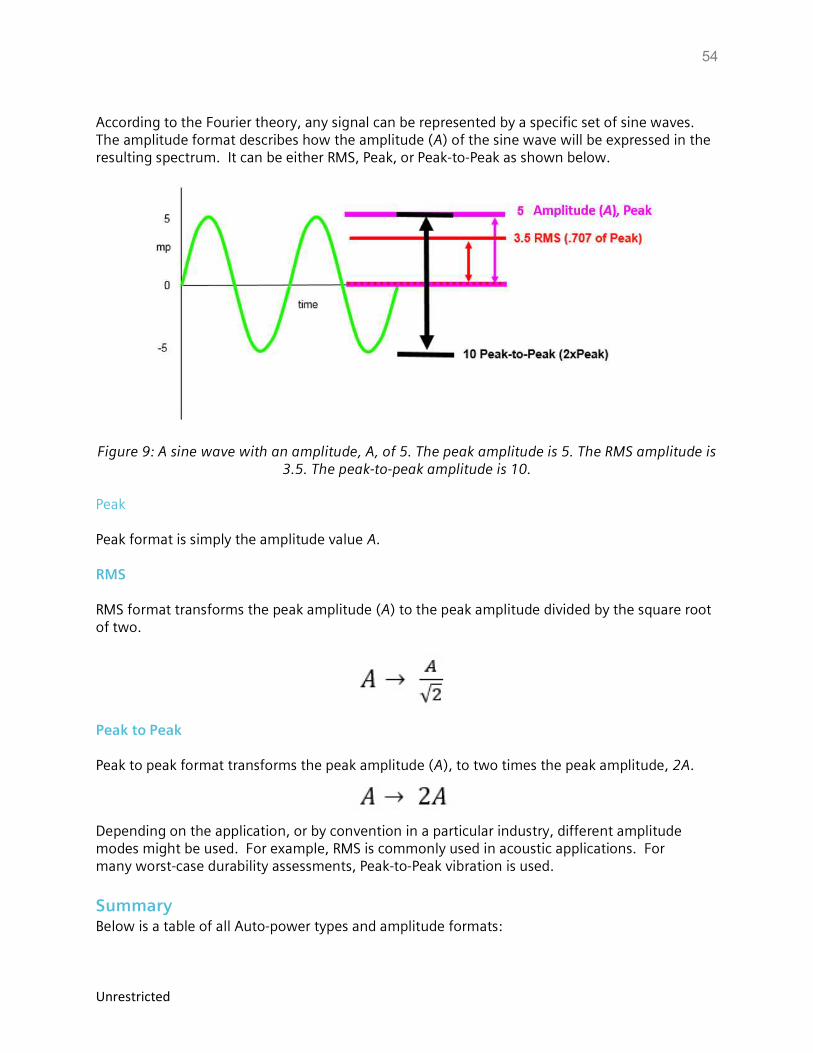
According to the Fourier theory, any signal can be represented by a specific set of sine waves. The amplitude format describes how the amplitude (A) of the sine wave will be expressed in the resulting spectrum. It can be either RMS, Peak, or Peak-to-Peak as shown below.

Figure 9: A sine wave with an amplitude, A, of 5. The peak amplitude is 5. The RMS amplitude is 3.5. The peak-to-peak amplitude is 10.

Peak Peak format is simply the amplitude value A. RMS RMS format transforms the peak amplitude (A) to the peak amplitude divided by the square root of two.

Peak to Peak Peak to peak format transforms the peak amplitude (A), to two times the peak amplitude, 2A.

Depending on the application, or by convention in a particular industry, different amplitude modes might be used. For example, RMS is commonly used in acoustic applications. For many worst-case durability assessments, Peak-to-Peak vibration is used.

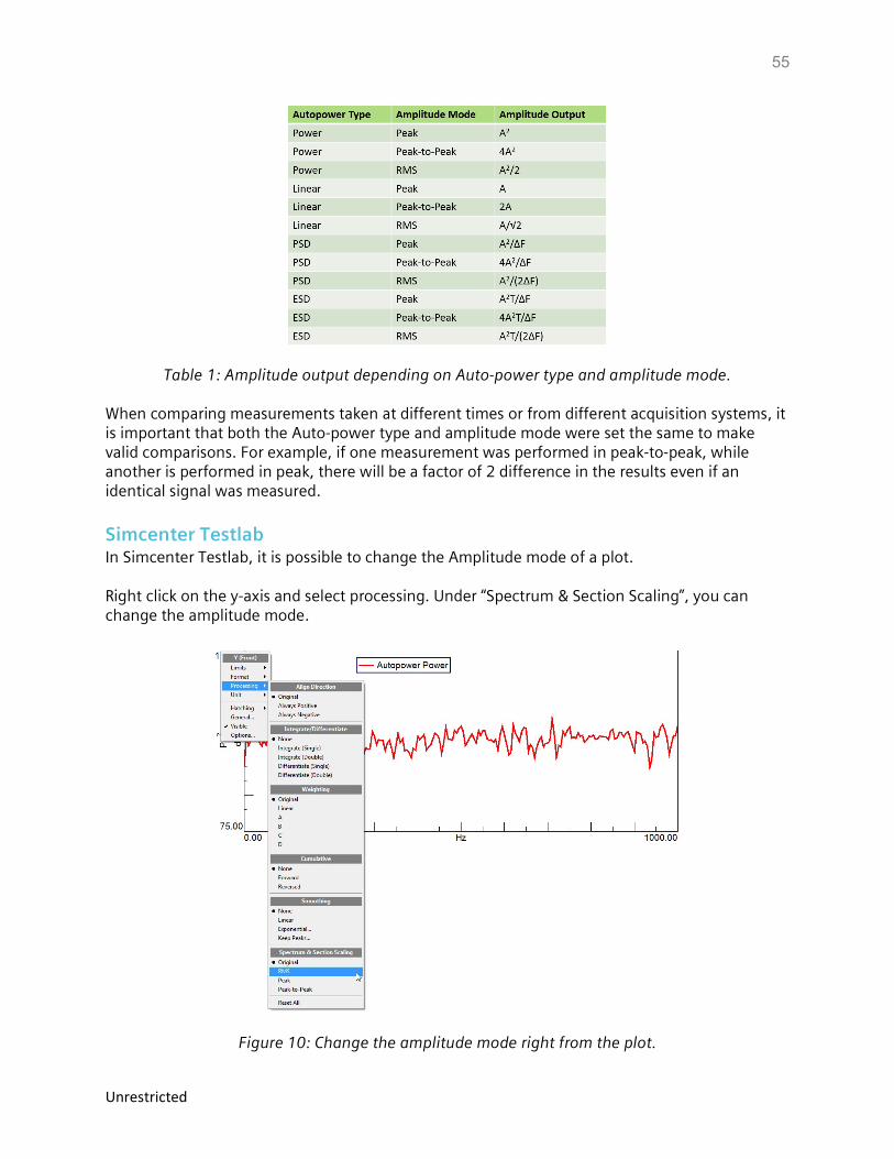
Summary Below is a table of all Auto-power types and amplitude formats:

55

Unrestricted

Table 1: Amplitude output depending on Auto-power type and amplitude mode. When comparing measurements taken at different times or from different acquisition systems, it is important that both the Auto-power type and amplitude mode were set the same to make valid comparisons. For example, if one measurement was performed in peak-to-peak, while another is performed in peak, there will be a factor of 2 difference in the results even if an identical signal was measured.

Simcenter Testlab In Simcenter Testlab, it is possible to change the Amplitude mode of a plot. Right click on the y-axis and select processing. Under “Spectrum & Section Scaling”, you can change the amplitude mode.

Figure 10: Change the amplitude mode right from the plot.

56

Unrestricted

Conclusion The amplitude of an Auto-power is a function of several variables: Auto-power type, Amplitude mode, the spectral resolution, and any window (like Hanning, Flattop, etc.) applied during the Fourier transformation. Some things to keep in mind: Auto-power power versus Auto-power linear - While squaring allows spectrums to be averaged for meaningful amplitude, the results squared units ("25 g2") can be confusing. The Auto-power linear takes the square root ("5 g").

Auto-power PSD - An Auto-power PSD is commonly used to quantify broadband random signals. The PSD normalizes the amplitudes for differing spectral resolutions to make comparison easier

Amplitude Mode - An Auto-power spectrum can be scaled whether it is RMS, Peak or Peak-to-Peak units. This is in addition to any changes in amplitude caused by selecting a particular Auto-power type.

57

Unrestricted

What is a Power Spectral Density (PSD)? A Power Spectral Density (PSD) is the measure of signal's power content versus frequency. A PSD is typically used to characterize broadband random signals. The amplitude of the PSD is normalized by the spectral resolution employed to digitize the signal. For vibration data, a PSD has amplitude units of g2/Hz. While this unit may not seem intuitive at first, it helps ensure that random data can be overlaid and compared independently of the spectral resolution used to measure the data. This article explains how this is done. To understand a Power Spectral Density (PSD), it is helpful to understand some limitations of an autopower function when analyzing data with differing spectral resolutions:

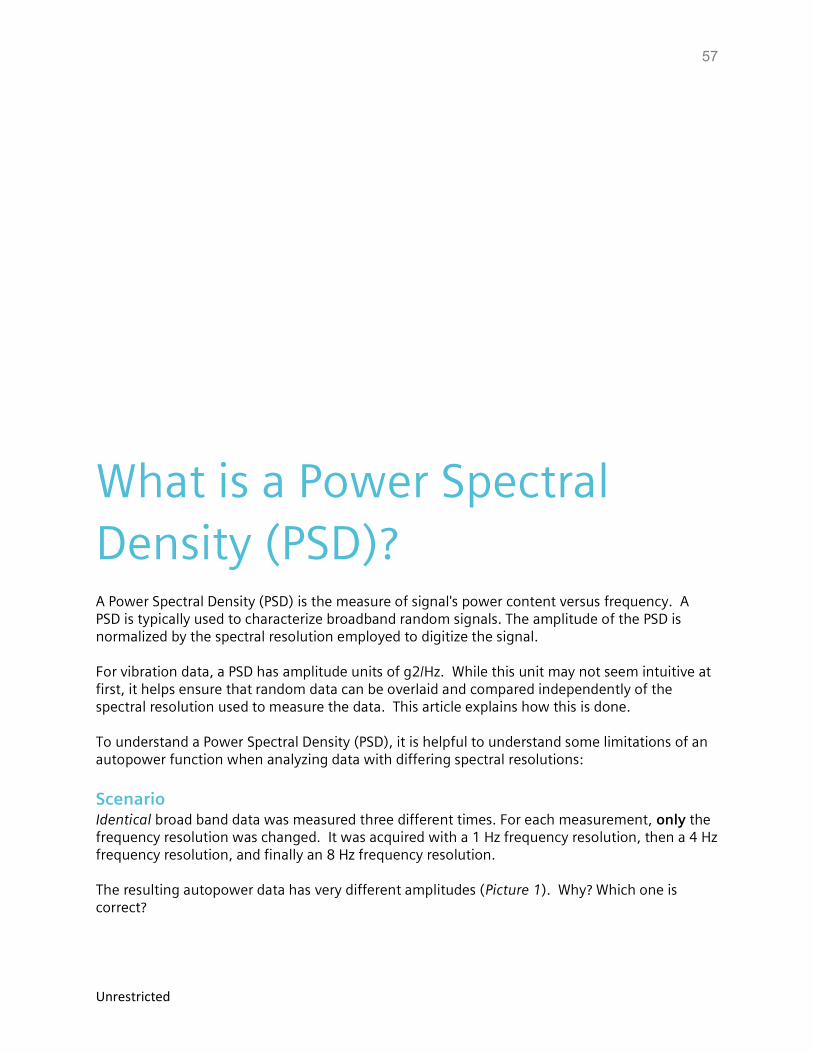
Scenario Identical broad band data was measured three different times. For each measurement, only the frequency resolution was changed. It was acquired with a 1 Hz frequency resolution, then a 4 Hz frequency resolution, and finally an 8 Hz frequency resolution. The resulting autopower data has very different amplitudes (Picture 1). Why? Which one is correct?

58

Unrestricted

Picture 1: Auto-powers of identical broadband data measured with 1 Hz spectral resolution

(red), 4 Hz spectral resolution (green) and 8 Hz spectral resolution (blue)

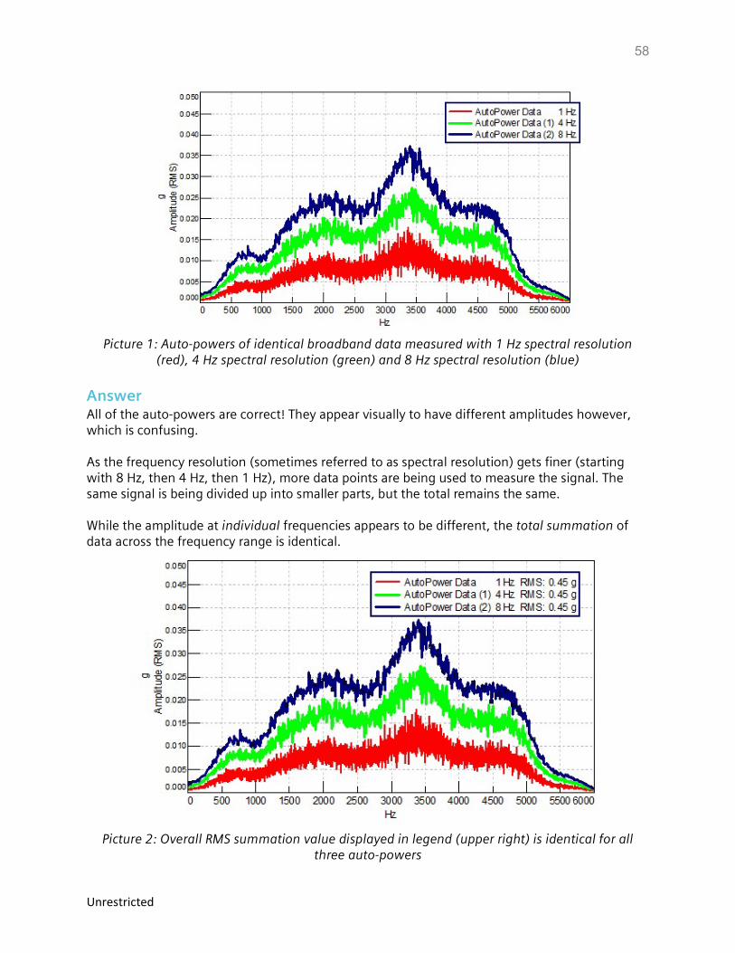
Answer All of the auto-powers are correct! They appear visually to have different amplitudes however, which is confusing. As the frequency resolution (sometimes referred to as spectral resolution) gets finer (starting with 8 Hz, then 4 Hz, then 1 Hz), more data points are being used to measure the signal. The same signal is being divided up into smaller parts, but the total remains the same. While the amplitude at individual frequencies appears to be different, the total summation of data across the frequency range is identical.

Picture 2: Overall RMS summation value displayed in legend (upper right) is identical for all

three auto-powers

59

Unrestricted

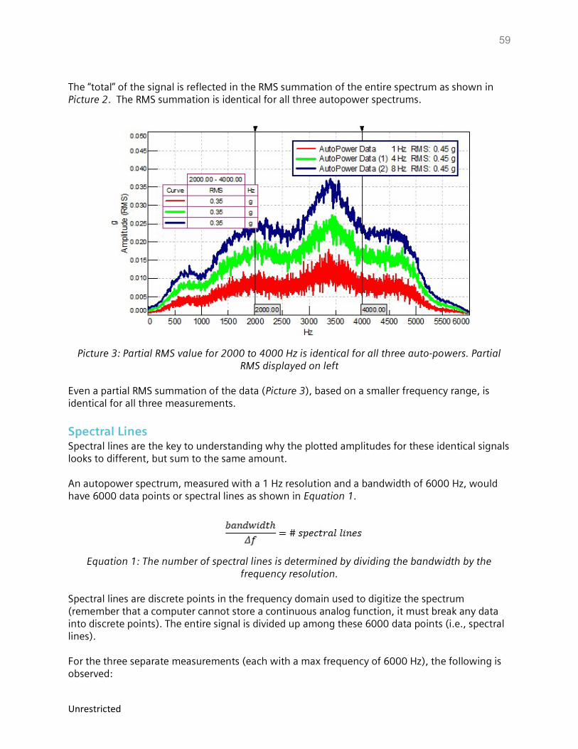
The “total” of the signal is reflected in the RMS summation of the entire spectrum as shown in Picture 2. The RMS summation is identical for all three autopower spectrums.

Picture 3: Partial RMS value for 2000 to 4000 Hz is identical for all three auto-powers. Partial

RMS displayed on left Even a partial RMS summation of the data (Picture 3), based on a smaller frequency range, is identical for all three measurements.

Spectral Lines Spectral lines are the key to understanding why the plotted amplitudes for these identical signals looks to different, but sum to the same amount. An autopower spectrum, measured with a 1 Hz resolution and a bandwidth of 6000 Hz, would have 6000 data points or spectral lines as shown in Equation 1.

Equation 1: The number of spectral lines is determined by dividing the bandwidth by the

frequency resolution. Spectral lines are discrete points in the frequency domain used to digitize the spectrum (remember that a computer cannot store a continuous analog function, it must break any data into discrete points). The entire signal is divided up among these 6000 data points (i.e., spectral lines). For the three separate measurements (each with a max frequency of 6000 Hz), the following is observed:

60

Unrestricted

1 Hz frequency resolution -> 6000 spectral lines -> lowest apparent amplitude 4 Hz frequency resolution -> 1500 spectral lines -> mid-range apparent amplitude 8 Hz frequency resolution -> 750 spectral lines -> highest apparent amplitude

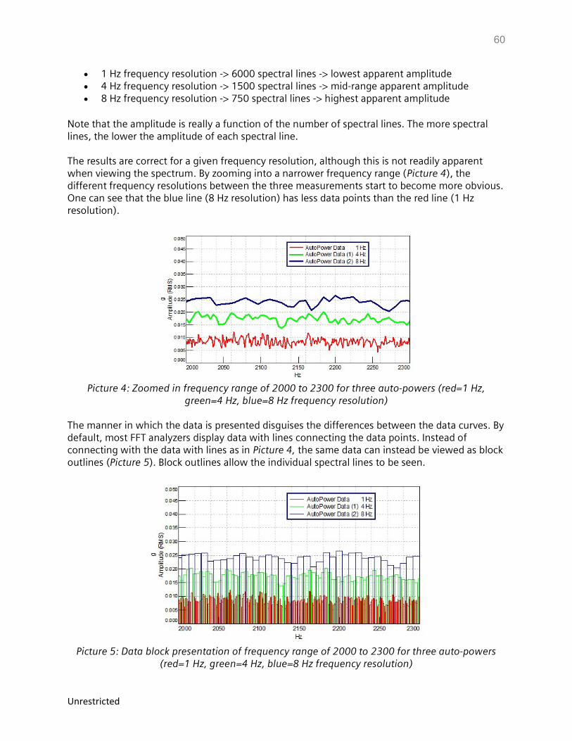
Note that the amplitude is really a function of the number of spectral lines. The more spectral lines, the lower the amplitude of each spectral line. The results are correct for a given frequency resolution, although this is not readily apparent when viewing the spectrum. By zooming into a narrower frequency range (Picture 4), the different frequency resolutions between the three measurements start to become more obvious. One can see that the blue line (8 Hz resolution) has less data points than the red line (1 Hz resolution).

Picture 4: Zoomed in frequency range of 2000 to 2300 for three auto-powers (red=1 Hz,

green=4 Hz, blue=8 Hz frequency resolution)

The manner in which the data is presented disguises the differences between the data curves. By default, most FFT analyzers display data with lines connecting the data points. Instead of connecting with the data with lines as in Picture 4, the same data can instead be viewed as block outlines (Picture 5). Block outlines allow the individual spectral lines to be seen.

Picture 5: Data block presentation of frequency range of 2000 to 2300 for three auto-powers

(red=1 Hz, green=4 Hz, blue=8 Hz frequency resolution)

61

Unrestricted

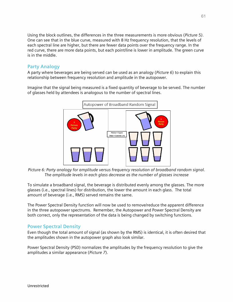
Using the block outlines, the differences in the three measurements is more obvious (Picture 5). One can see that in the blue curve, measured with 8 Hz frequency resolution, that the levels of each spectral line are higher, but there are fewer data points over the frequency range. In the red curve, there are more data points, but each point/line is lower in amplitude. The green curve is in the middle.

Party Analogy A party where beverages are being served can be used as an analogy (Picture 6) to explain this relationship between frequency resolution and amplitude in the autopower. Imagine that the signal being measured is a fixed quantity of beverage to be served. The number of glasses held by attendees is analogous to the number of spectral lines.

Picture 6: Party analogy for amplitude versus frequency resolution of broadband random signal.

The amplitude levels in each glass decrease as the number of glasses increase

To simulate a broadband signal, the beverage is distributed evenly among the glasses. The more glasses (i.e., spectral lines) for distribution, the lower the amount in each glass. The total amount of beverage (i.e., RMS) served remains the same. The Power Spectral Density function will now be used to remove/reduce the apparent difference in the three autopower spectrums. Remember, the Autopower and Power Spectral Density are both correct, only the representation of the data is being changed by switching functions.

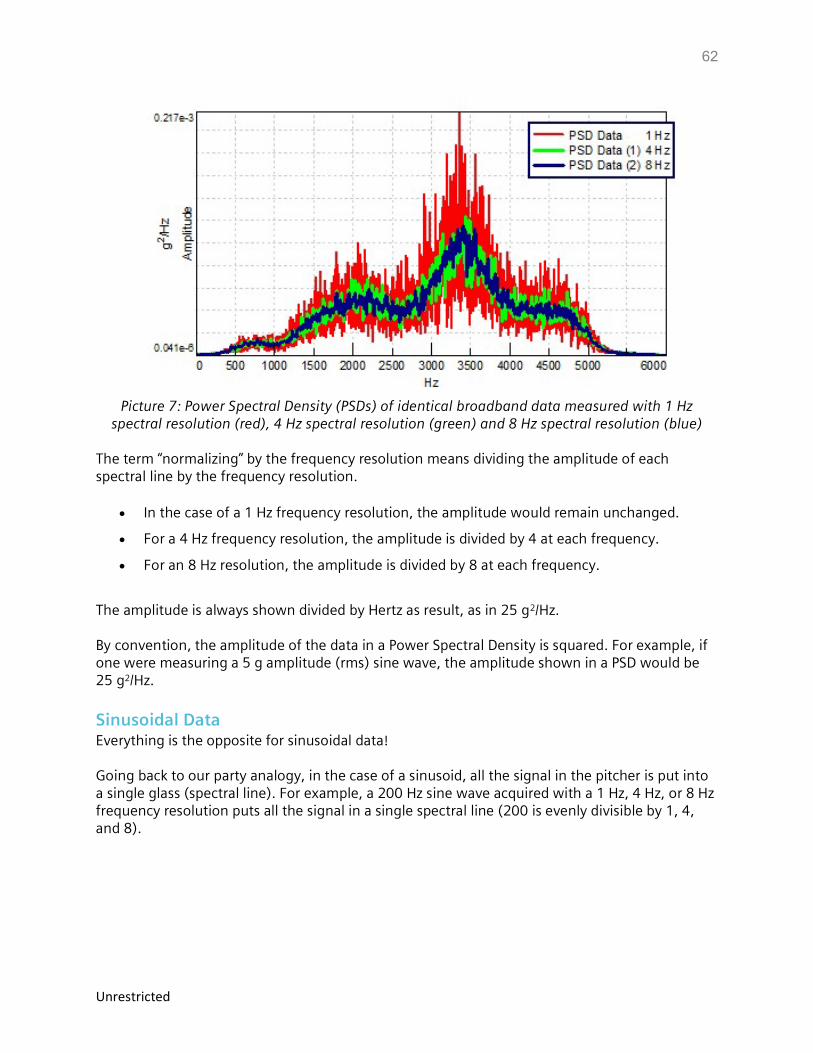
Power Spectral Density Even though the total amount of signal (as shown by the RMS) is identical, it is often desired that the amplitudes shown in the autopower graph also look similar. Power Spectral Density (PSD) normalizes the amplitudes by the frequency resolution to give the amplitudes a similar appearance (Picture 7).

62

Unrestricted

Picture 7: Power Spectral Density (PSDs) of identical broadband data measured with 1 Hz

spectral resolution (red), 4 Hz spectral resolution (green) and 8 Hz spectral resolution (blue) The term “normalizing” by the frequency resolution means dividing the amplitude of each spectral line by the frequency resolution.

In the case of a 1 Hz frequency resolution, the amplitude would remain unchanged.

For a 4 Hz frequency resolution, the amplitude is divided by 4 at each frequency.

For an 8 Hz resolution, the amplitude is divided by 8 at each frequency.

The amplitude is always shown divided by Hertz as result, as in 25 g2/Hz. By convention, the amplitude of the data in a Power Spectral Density is squared. For example, if one were measuring a 5 g amplitude (rms) sine wave, the amplitude shown in a PSD would be 25 g2/Hz.

Sinusoidal Data Everything is the opposite for sinusoidal data! Going back to our party analogy, in the case of a sinusoid, all the signal in the pitcher is put into a single glass (spectral line). For example, a 200 Hz sine wave acquired with a 1 Hz, 4 Hz, or 8 Hz frequency resolution puts all the signal in a single spectral line (200 is evenly divisible by 1, 4, and 8).

63

Unrestricted

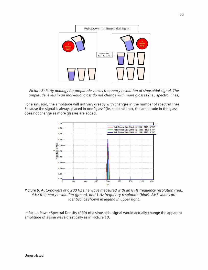
Picture 8: Party analogy for amplitude versus frequency resolution of sinusoidal signal. The amplitude levels in an individual glass do not change with more glasses (i.e., spectral lines)

For a sinusoid, the amplitude will not vary greatly with changes in the number of spectral lines. Because the signal is always placed in one “glass” (ie, spectral line), the amplitude in the glass does not change as more glasses are added.

Picture 9: Auto-powers of a 200 Hz sine wave measured with an 8 Hz frequency resolution (red),

4 Hz frequency resolution (green), and 1 Hz frequency resolution (blue). RMS values are identical as shown in legend in upper right.

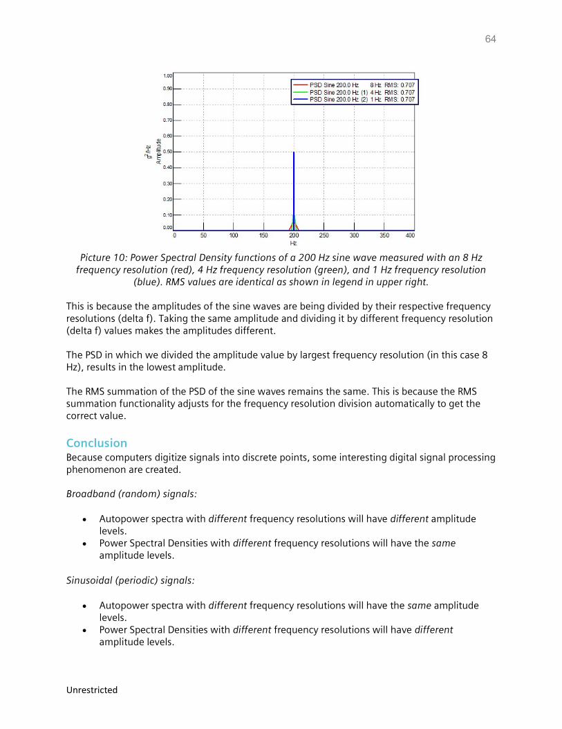
In fact, a Power Spectral Density (PSD) of a sinusoidal signal would actually change the apparent amplitude of a sine wave drastically as in Picture 10.

64

Unrestricted

Picture 10: Power Spectral Density functions of a 200 Hz sine wave measured with an 8 Hz

frequency resolution (red), 4 Hz frequency resolution (green), and 1 Hz frequency resolution (blue). RMS values are identical as shown in legend in upper right.

This is because the amplitudes of the sine waves are being divided by their respective frequency resolutions (delta f). Taking the same amplitude and dividing it by different frequency resolution (delta f) values makes the amplitudes different. The PSD in which we divided the amplitude value by largest frequency resolution (in this case 8 Hz), results in the lowest amplitude. The RMS summation of the PSD of the sine waves remains the same. This is because the RMS summation functionality adjusts for the frequency resolution division automatically to get the correct value.

Conclusion Because computers digitize signals into discrete points, some interesting digital signal processing phenomenon are created. Broadband (random) signals:

Autopower spectra with different frequency resolutions will have different amplitude levels.

Power Spectral Densities with different frequency resolutions will have the same amplitude levels.

Sinusoidal (periodic) signals:

Autopower spectra with different frequency resolutions will have the same amplitude levels.

Power Spectral Densities with different frequency resolutions will have different amplitude levels.

65

Unrestricted

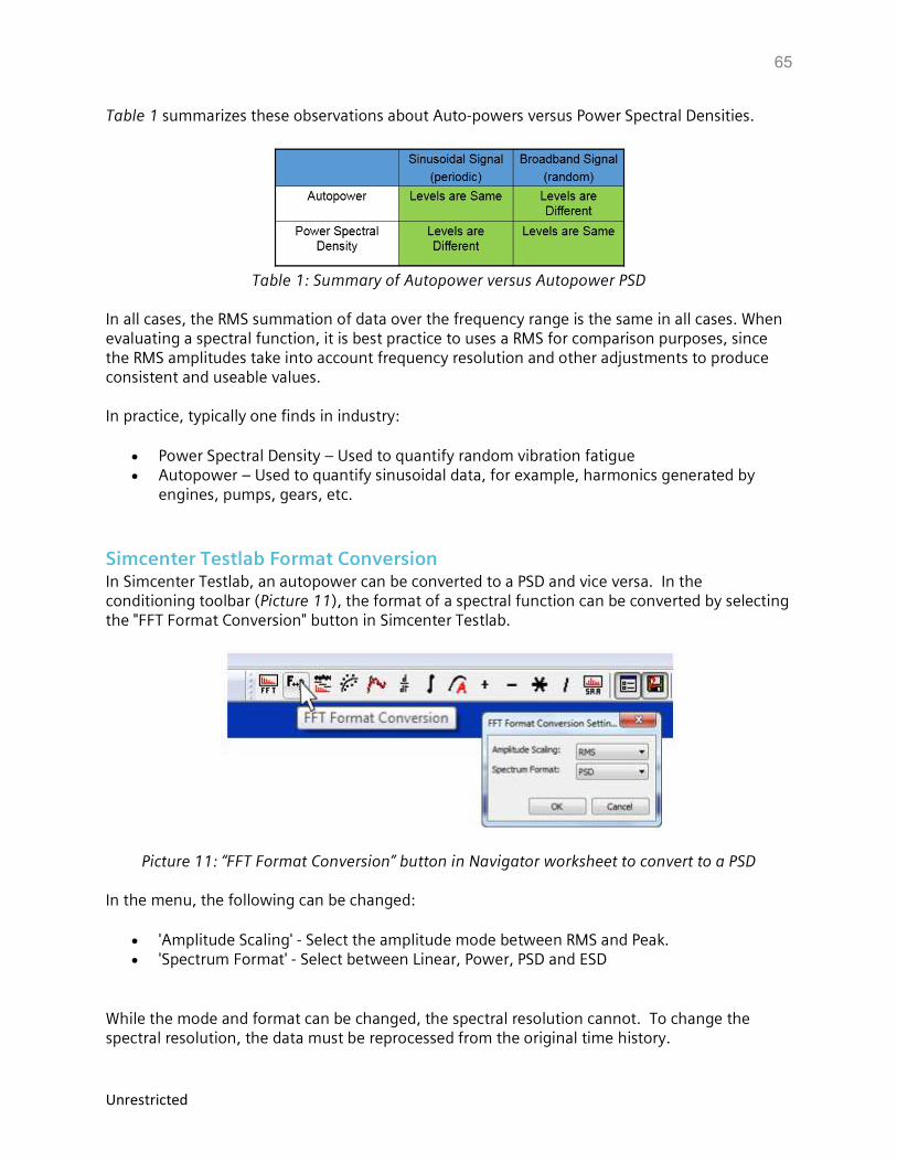
Table 1 summarizes these observations about Auto-powers versus Power Spectral Densities.

Table 1: Summary of Autopower versus Autopower PSD

In all cases, the RMS summation of data over the frequency range is the same in all cases. When evaluating a spectral function, it is best practice to uses a RMS for comparison purposes, since the RMS amplitudes take into account frequency resolution and other adjustments to produce consistent and useable values. In practice, typically one finds in industry:

Power Spectral Density – Used to quantify random vibration fatigue Autopower – Used to quantify sinusoidal data, for example, harmonics generated by

engines, pumps, gears, etc.

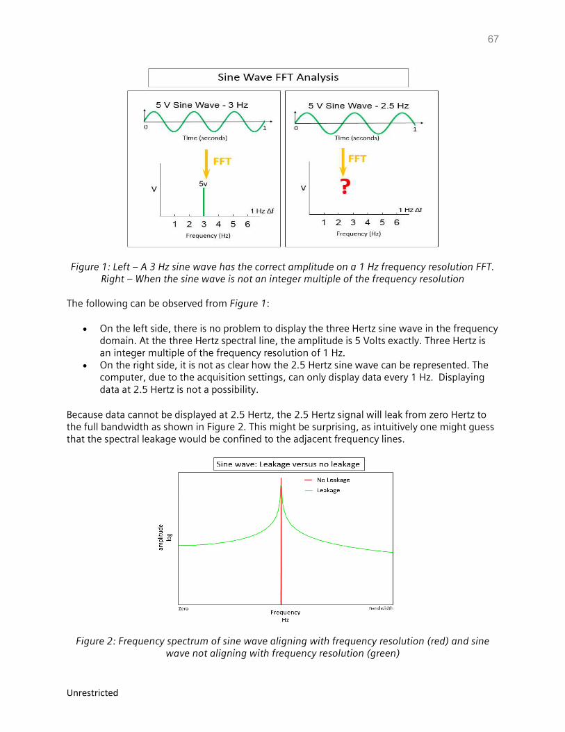
Simcenter Testlab Format Conversion In Simcenter Testlab, an autopower can be converted to a PSD and vice versa. In the conditioning toolbar (Picture 11), the format of a spectral function can be converted by selecting the "FFT Format Conversion" button in Simcenter Testlab.

Picture 11: “FFT Format Conversion” button in Navigator worksheet to convert to a PSD In the menu, the following can be changed:

'Amplitude Scaling' - Select the amplitude mode between RMS and Peak. 'Spectrum Format' - Select between Linear, Power, PSD and ESD

While the mode and format can be changed, the spectral resolution cannot. To change the spectral resolution, the data must be reprocessed from the original time history.

66

Unrestricted

Windows and Spectral Leakage

Windows and Leakage Spectral leakage is a problem that arises in the digital processing of signals. Leakage causes the signal levels to be reduced and redistributed over a broad frequency range, which must be addressed in order to analyze digital signals properly. This article explains what causes leakage, what it looks like, and how to use windows to mitigate the effects of leakage by smoothing a signal in the time domain before performing a Fourier Transform.

Example with Sine Wave Take an example with a sine wave. Suppose your analyzer is setup to perform a Fast Fourier Transform (FFT) that will result in a 1 Hz frequency resolution as shown in Figure 1. The frequency resolution setting means that the computer can display only every 1 Hz.

67

Unrestricted

Figure 1: Left – A 3 Hz sine wave has the correct amplitude on a 1 Hz frequency resolution FFT. Right – When the sine wave is not an integer multiple of the frequency resolution

The following can be observed from Figure 1:

On the left side, there is no problem to display the three Hertz sine wave in the frequency domain. At the three Hertz spectral line, the amplitude is 5 Volts exactly. Three Hertz is an integer multiple of the frequency resolution of 1 Hz.

On the right side, it is not as clear how the 2.5 Hertz sine wave can be represented. The computer, due to the acquisition settings, can only display data every 1 Hz. Displaying data at 2.5 Hertz is not a possibility.

Because data cannot be displayed at 2.5 Hertz, the 2.5 Hertz signal will leak from zero Hertz to the full bandwidth as shown in Figure 2. This might be surprising, as intuitively one might guess that the spectral leakage would be confined to the adjacent frequency lines.

Figure 2: Frequency spectrum of sine wave aligning with frequency resolution (red) and sine wave not aligning with frequency resolution (green)

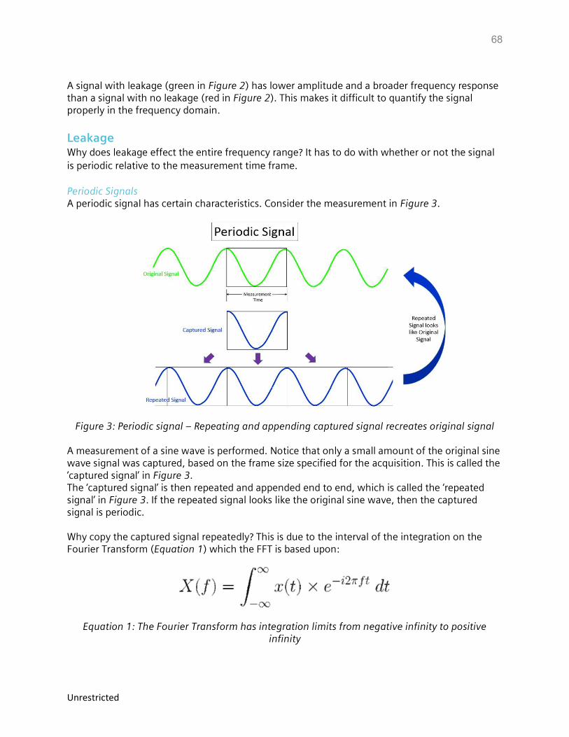
68

Unrestricted

A signal with leakage (green in Figure 2) has lower amplitude and a broader frequency response than a signal with no leakage (red in Figure 2). This makes it difficult to quantify the signal properly in the frequency domain.

Leakage Why does leakage effect the entire frequency range? It has to do with whether or not the signal is periodic relative to the measurement time frame. Periodic Signals A periodic signal has certain characteristics. Consider the measurement in Figure 3.

Figure 3: Periodic signal – Repeating and appending captured signal recreates original signal A measurement of a sine wave is performed. Notice that only a small amount of the original sine wave signal was captured, based on the frame size specified for the acquisition. This is called the ‘captured signal’ in Figure 3. The ‘captured signal’ is then repeated and appended end to end, which is called the ‘repeated signal’ in Figure 3. If the repeated signal looks like the original sine wave, then the captured signal is periodic. Why copy the captured signal repeatedly? This is due to the interval of the integration on the Fourier Transform (Equation 1) which the FFT is based upon:

Equation 1: The Fourier Transform has integration limits from negative infinity to positive infinity

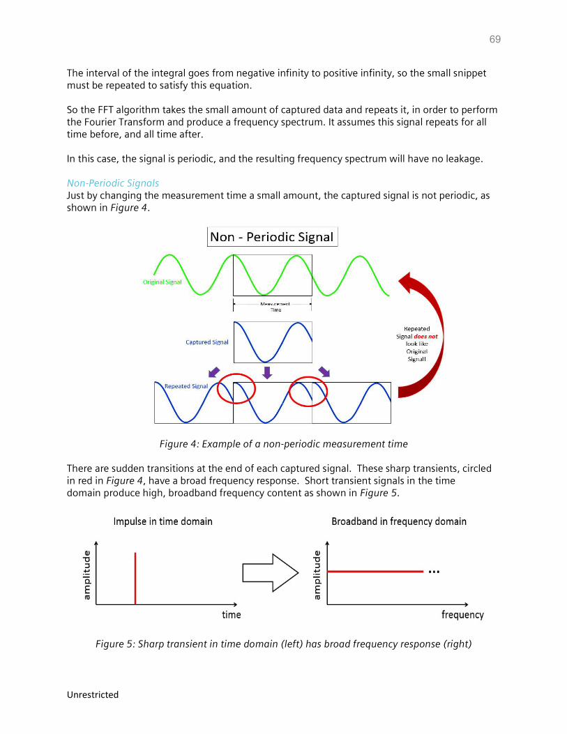
69

Unrestricted

The interval of the integral goes from negative infinity to positive infinity, so the small snippet must be repeated to satisfy this equation. So the FFT algorithm takes the small amount of captured data and repeats it, in order to perform the Fourier Transform and produce a frequency spectrum. It assumes this signal repeats for all time before, and all time after. In this case, the signal is periodic, and the resulting frequency spectrum will have no leakage. Non-Periodic Signals Just by changing the measurement time a small amount, the captured signal is not periodic, as shown in Figure 4.

Figure 4: Example of a non-periodic measurement time There are sudden transitions at the end of each captured signal. These sharp transients, circled in red in Figure 4, have a broad frequency response. Short transient signals in the time domain produce high, broadband frequency content as shown in Figure 5.

Figure 5: Sharp transient in time domain (left) has broad frequency response (right)

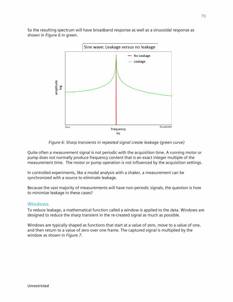
70

Unrestricted

So the resulting spectrum will have broadband response as well as a sinusoidal response as shown in Figure 6 in green.

Figure 6: Sharp transients in repeated signal create leakage (green curve)

Quite often a measurement signal is not periodic with the acquisition time. A running motor or pump does not normally produce frequency content that is an exact integer multiple of the measurement time. The motor or pump operation is not influenced by the acquisition settings. In controlled experiments, like a modal analysis with a shaker, a measurement can be synchronized with a source to eliminate leakage. Because the vast majority of measurements will have non-periodic signals, the question is how to minimize leakage in these cases?

Windows To reduce leakage, a mathematical function called a window is applied to the data. Windows are designed to reduce the sharp transient in the re-created signal as much as possible. Windows are typically shaped as functions that start at a value of zero, move to a value of one, and then return to a value of zero over one frame. The captured signal is multiplied by the window as shown in Figure 7.

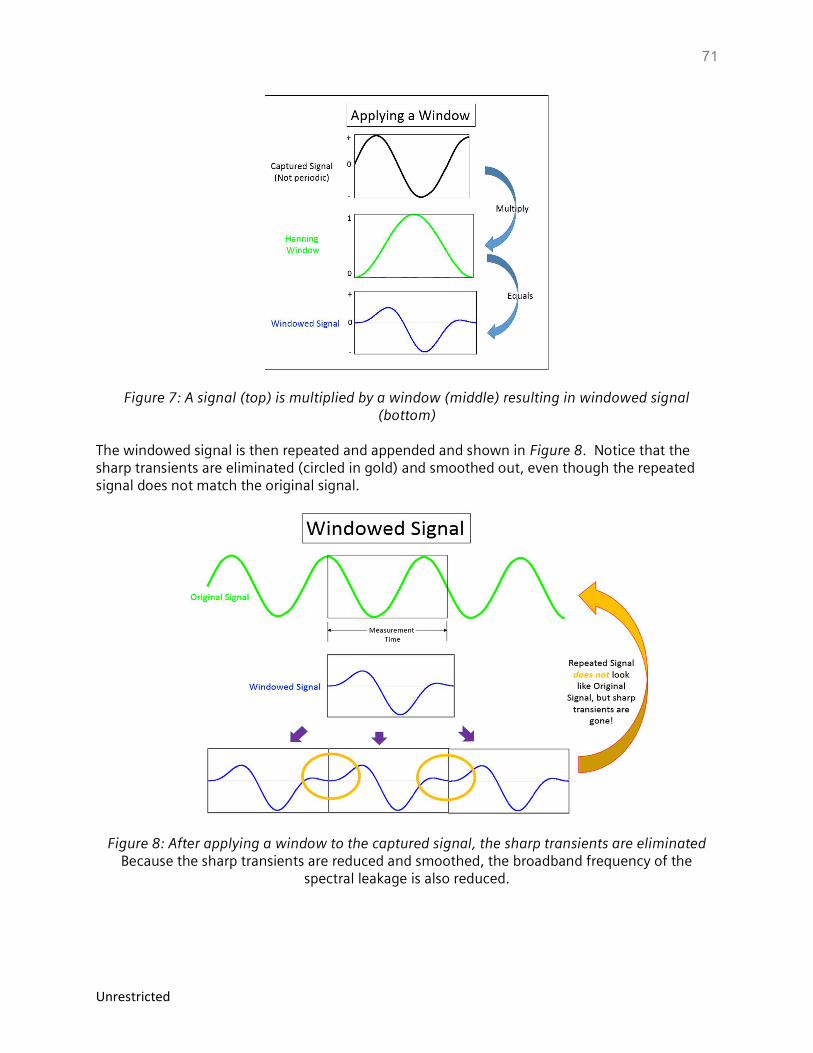
71

Unrestricted

Figure 7: A signal (top) is multiplied by a window (middle) resulting in windowed signal (bottom)

The windowed signal is then repeated and appended and shown in Figure 8. Notice that the sharp transients are eliminated (circled in gold) and smoothed out, even though the repeated signal does not match the original signal.

Figure 8: After applying a window to the captured signal, the sharp transients are eliminated Because the sharp transients are reduced and smoothed, the broadband frequency of the

spectral leakage is also reduced.

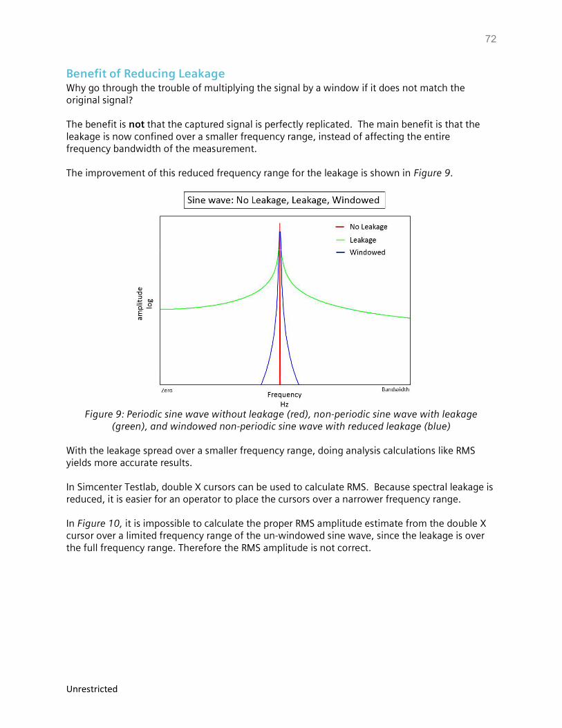
72

Unrestricted

Benefit of Reducing Leakage Why go through the trouble of multiplying the signal by a window if it does not match the original signal? The benefit is not that the captured signal is perfectly replicated. The main benefit is that the leakage is now confined over a smaller frequency range, instead of affecting the entire frequency bandwidth of the measurement. The improvement of this reduced frequency range for the leakage is shown in Figure 9.

Figure 9: Periodic sine wave without leakage (red), non-periodic sine wave with leakage

(green), and windowed non-periodic sine wave with reduced leakage (blue)

With the leakage spread over a smaller frequency range, doing analysis calculations like RMS yields more accurate results. In Simcenter Testlab, double X cursors can be used to calculate RMS. Because spectral leakage is reduced, it is easier for an operator to place the cursors over a narrower frequency range. In Figure 10, it is impossible to calculate the proper RMS amplitude estimate from the double X cursor over a limited frequency range of the un-windowed sine wave, since the leakage is over the full frequency range. Therefore the RMS amplitude is not correct.

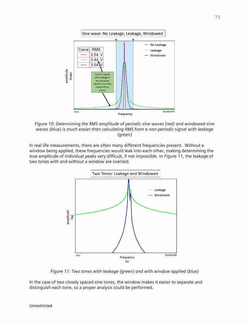
73

Unrestricted

Figure 10: Determining the RMS amplitude of periodic sine waves (red) and windowed sine waves (blue) is much easier than calculating RMS from a non-periodic signal with leakage

(green) In real life measurements, there are often many different frequencies present. Without a window being applied, these frequencies would leak into each other, making determining the true amplitude of individual peaks very difficult, if not impossible. In Figure 11, the leakage of two tones with and without a window are overlaid.

Figure 11: Two tones with leakage (green) and with window applied (blue) In the case of two closely spaced sine tones, the window makes it easier to separate and distinguish each tone, so a proper analysis could be performed.

74

Unrestricted

Window Types There are many different windows, each optimized for a particular situation. Some windows include:

Hanning – Used for general data analysis, good tradeoff between frequency and amplitude accuracy

Flattop – Excellent accuracy for amplitude, often used in calibration

Tukey – Used for transient events

Exponential – Used in impact hammer modal testing, be careful of adding artificial damping to measurement

Uniform – Another way of saying “no window”

Depending on the measurement situation, the appropriate window can be applied.

Conclusions Spectral leakage is a challenge in digital signal processing, which can be addressed by applying windows:

Leakage is created by a digital Fourier transform of non-periodic data

Leakage causes a redistribution of the signal over the entire frequency range of the measurement

Windows can help minimize the effects of leakage by smoothing the time domain signal, but cannot entirely eliminate leakage

75

Unrestricted

Window Types

Window Types There are several different types of windows used to reduce spectral leakage when performing a Fourier Transform on time data and converting it into the frequency domain. Each window is designed with a specific purpose. The details and tradeoffs of the following windows will be covered in this article:

Hanning Flattop Uniform Tukey Exponential

Throughout the article, the term measurement time refers to the amount of time to acquire a single average or FFT of data. Measurement time can also be referred to as frame size.

Periodic versus Non-Periodic Background Before delving into the specifics of each window, it is helpful to understand spectral leakage in light of signals captured in a periodic or non-periodic manner. Any signal data, based on how it is captured by the measurement time, is either periodic or non-periodic. When performing a Fourier Transform on measurement data, a window affects periodic and non-periodic data differently:

Periodic (No Window needed): A signal captured in a periodic manner does not require a window, and a resulting Fourier Transform has no leakage. Applying a window alters the

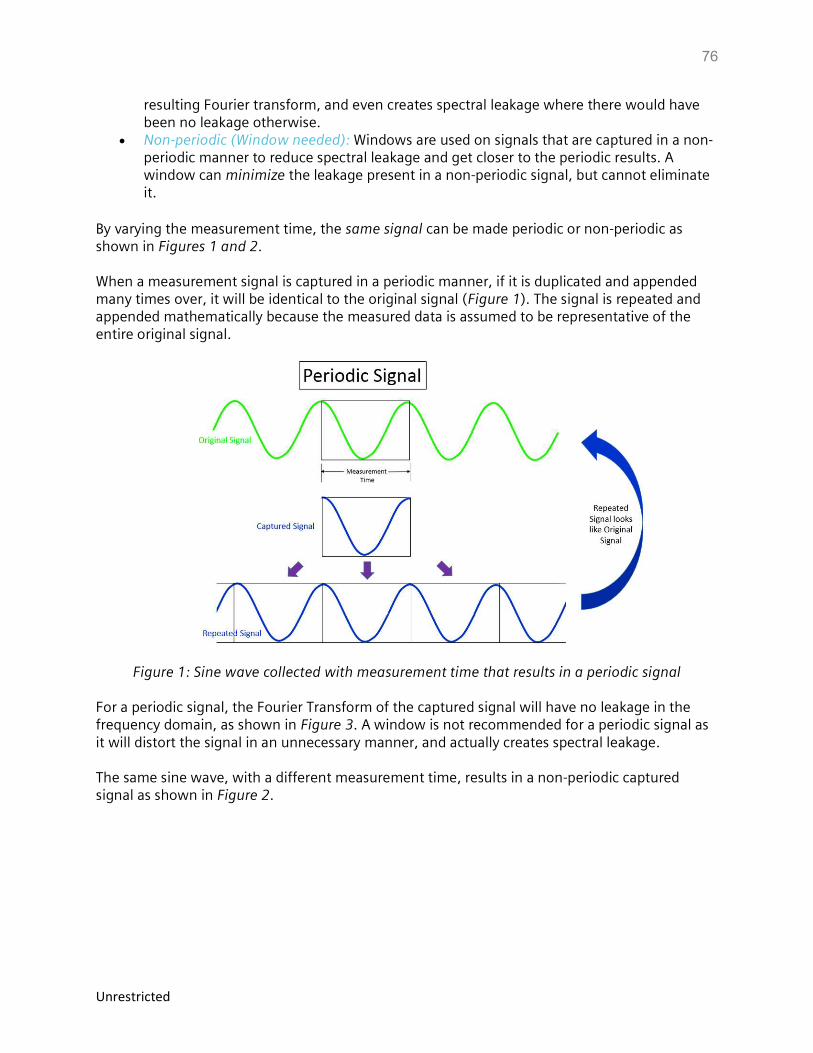
76

Unrestricted

resulting Fourier transform, and even creates spectral leakage where there would have been no leakage otherwise.

Non-periodic (Window needed): Windows are used on signals that are captured in a non-periodic manner to reduce spectral leakage and get closer to the periodic results. A window can minimize the leakage present in a non-periodic signal, but cannot eliminate it.

By varying the measurement time, the same signal can be made periodic or non-periodic as shown in Figures 1 and 2. When a measurement signal is captured in a periodic manner, if it is duplicated and appended many times over, it will be identical to the original signal (Figure 1). The signal is repeated and appended mathematically because the measured data is assumed to be representative of the entire original signal.

Figure 1: Sine wave collected with measurement time that results in a periodic signal For a periodic signal, the Fourier Transform of the captured signal will have no leakage in the frequency domain, as shown in Figure 3. A window is not recommended for a periodic signal as it will distort the signal in an unnecessary manner, and actually creates spectral leakage. The same sine wave, with a different measurement time, results in a non-periodic captured signal as shown in Figure 2.

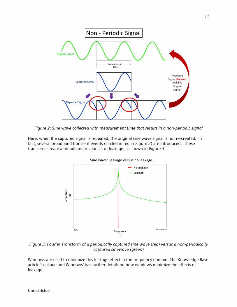
77

Unrestricted

Figure 2: Sine wave collected with measurement time that results in a non-periodic signal Here, when the captured signal is repeated, the original sine wave signal is not re-created. In fact, several broadband transient events (circled in red in Figure 2) are introduced. These transients create a broadband response, or leakage, as shown in Figure 3.

Figure 3: Fourier Transform of a periodically captured sine wave (red) versus a non-periodically captured sinewave (green)

Windows are used to minimize this leakage effect in the frequency domain. The Knowledge Base article 'Leakage and Windows' has further details on how windows minimize the effects of leakage.

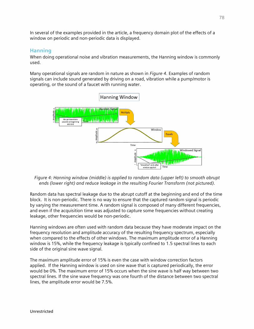
78

Unrestricted

In several of the examples provided in the article, a frequency domain plot of the effects of a window on periodic and non-periodic data is displayed.

Hanning When doing operational noise and vibration measurements, the Hanning window is commonly used. Many operational signals are random in nature as shown in Figure 4. Examples of random signals can include sound generated by driving on a road, vibration while a pump/motor is operating, or the sound of a faucet with running water.

Figure 4: Hanning window (middle) is applied to random data (upper left) to smooth abrupt ends (lower right) and reduce leakage in the resulting Fourier Transform (not pictured).

Random data has spectral leakage due to the abrupt cutoff at the beginning and end of the time block. It is non-periodic. There is no way to ensure that the captured random signal is periodic by varying the measurement time. A random signal is composed of many different frequencies, and even if the acquisition time was adjusted to capture some frequencies without creating leakage, other frequencies would be non-periodic. Hanning windows are often used with random data because they have moderate impact on the frequency resolution and amplitude accuracy of the resulting frequency spectrum, especially when compared to the effects of other windows. The maximum amplitude error of a Hanning window is 15%, while the frequency leakage is typically confined to 1.5 spectral lines to each side of the original sine wave signal. The maximum amplitude error of 15% is even the case with window correction factors applied. If the Hanning window is used on sine wave that is captured periodically, the error would be 0%. The maximum error of 15% occurs when the sine wave is half way between two spectral lines. If the sine wave frequency was one fourth of the distance between two spectral lines, the amplitude error would be 7.5%.

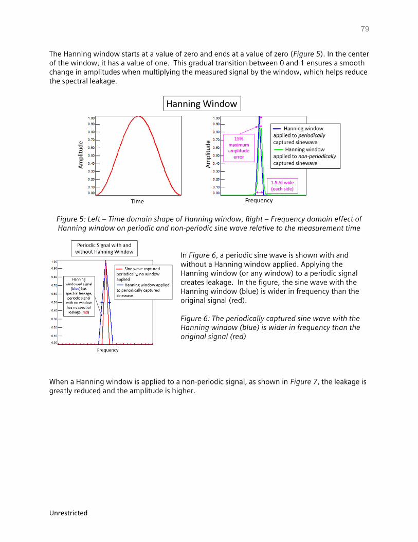
79

Unrestricted

The Hanning window starts at a value of zero and ends at a value of zero (Figure 5). In the center of the window, it has a value of one. This gradual transition between 0 and 1 ensures a smooth change in amplitudes when multiplying the measured signal by the window, which helps reduce the spectral leakage.

Figure 5: Left – Time domain shape of Hanning window, Right – Frequency domain effect of Hanning window on periodic and non-periodic sine wave relative to the measurement time

In Figure 6, a periodic sine wave is shown with and without a Hanning window applied. Applying the Hanning window (or any window) to a periodic signal creates leakage. In the figure, the sine wave with the Hanning window (blue) is wider in frequency than the original signal (red). Figure 6: The periodically captured sine wave with the Hanning window (blue) is wider in frequency than the original signal (red)

When a Hanning window is applied to a non-periodic signal, as shown in Figure 7, the leakage is greatly reduced and the amplitude is higher.

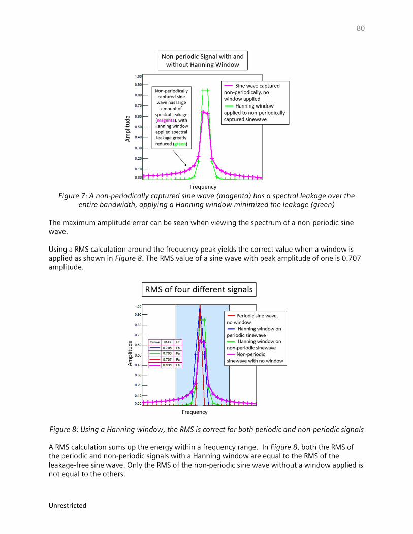
80

Unrestricted

Figure 7: A non-periodically captured sine wave (magenta) has a spectral leakage over the

entire bandwidth, applying a Hanning window minimized the leakage (green) The maximum amplitude error can be seen when viewing the spectrum of a non-periodic sine wave. Using a RMS calculation around the frequency peak yields the correct value when a window is applied as shown in Figure 8. The RMS value of a sine wave with peak amplitude of one is 0.707 amplitude.

Figure 8: Using a Hanning window, the RMS is correct for both periodic and non-periodic signals A RMS calculation sums up the energy within a frequency range. In Figure 8, both the RMS of the periodic and non-periodic signals with a Hanning window are equal to the RMS of the leakage-free sine wave. Only the RMS of the non-periodic sine wave without a window applied is not equal to the others.

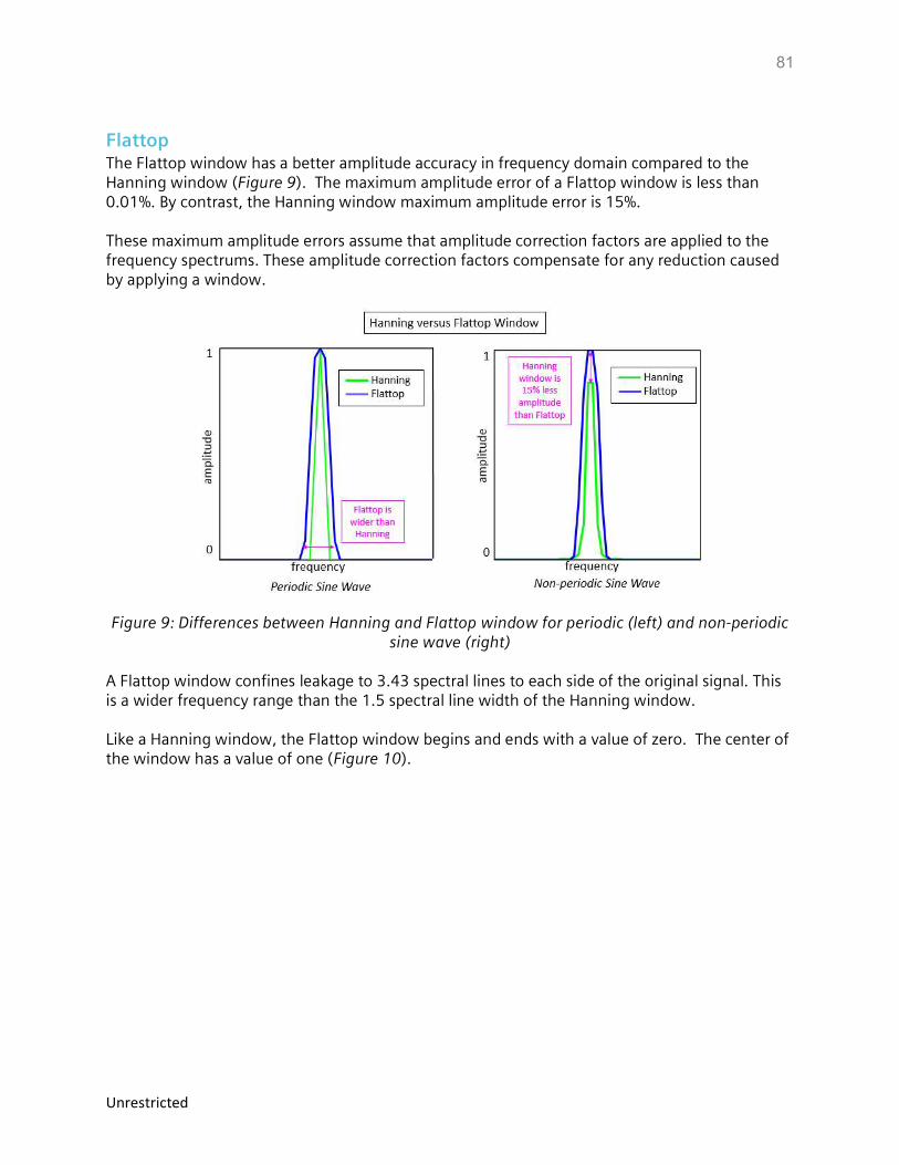
81

Unrestricted

Flattop The Flattop window has a better amplitude accuracy in frequency domain compared to the Hanning window (Figure 9). The maximum amplitude error of a Flattop window is less than 0.01%. By contrast, the Hanning window maximum amplitude error is 15%. These maximum amplitude errors assume that amplitude correction factors are applied to the frequency spectrums. These amplitude correction factors compensate for any reduction caused by applying a window.

Figure 9: Differences between Hanning and Flattop window for periodic (left) and non-periodic sine wave (right)

A Flattop window confines leakage to 3.43 spectral lines to each side of the original signal. This is a wider frequency range than the 1.5 spectral line width of the Hanning window. Like a Hanning window, the Flattop window begins and ends with a value of zero. The center of the window has a value of one (Figure 10).

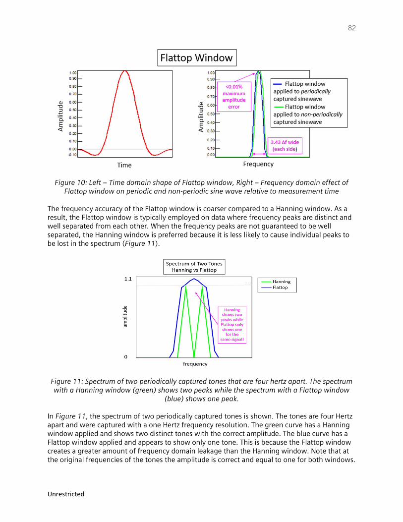
82

Unrestricted

Figure 10: Left – Time domain shape of Flattop window, Right – Frequency domain effect of Flattop window on periodic and non-periodic sine wave relative to measurement time

The frequency accuracy of the Flattop window is coarser compared to a Hanning window. As a result, the Flattop window is typically employed on data where frequency peaks are distinct and well separated from each other. When the frequency peaks are not guaranteed to be well separated, the Hanning window is preferred because it is less likely to cause individual peaks to be lost in the spectrum (Figure 11).

Figure 11: Spectrum of two periodically captured tones that are four hertz apart. The spectrum with a Hanning window (green) shows two peaks while the spectrum with a Flattop window

(blue) shows one peak.

In Figure 11, the spectrum of two periodically captured tones is shown. The tones are four Hertz apart and were captured with a one Hertz frequency resolution. The green curve has a Hanning window applied and shows two distinct tones with the correct amplitude. The blue curve has a Flattop window applied and appears to show only one tone. This is because the Flattop window creates a greater amount of frequency domain leakage than the Hanning window. Note that at the original frequencies of the tones the amplitude is correct and equal to one for both windows.

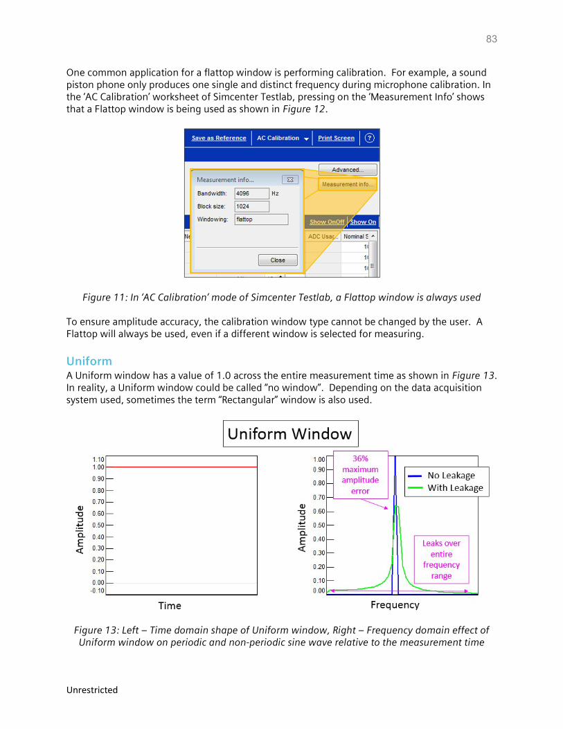
83

Unrestricted

One common application for a flattop window is performing calibration. For example, a sound piston phone only produces one single and distinct frequency during microphone calibration. In the ‘AC Calibration’ worksheet of Simcenter Testlab, pressing on the ‘Measurement Info’ shows that a Flattop window is being used as shown in Figure 12.

Figure 11: In ‘AC Calibration’ mode of Simcenter Testlab, a Flattop window is always used To ensure amplitude accuracy, the calibration window type cannot be changed by the user. A Flattop will always be used, even if a different window is selected for measuring.

Uniform A Uniform window has a value of 1.0 across the entire measurement time as shown in Figure 13. In reality, a Uniform window could be called “no window”. Depending on the data acquisition system used, sometimes the term “Rectangular” window is also used.

Figure 13: Left – Time domain shape of Uniform window, Right – Frequency domain effect of Uniform window on periodic and non-periodic sine wave relative to the measurement time

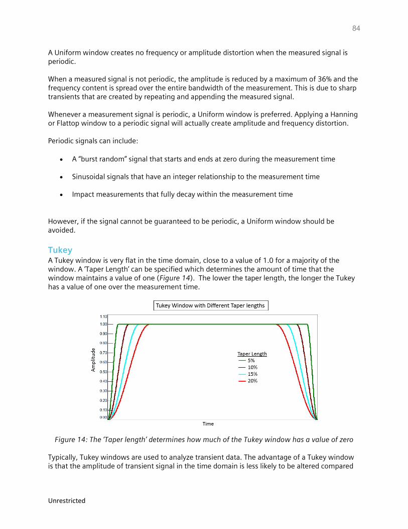
84

Unrestricted

A Uniform window creates no frequency or amplitude distortion when the measured signal is periodic. When a measured signal is not periodic, the amplitude is reduced by a maximum of 36% and the frequency content is spread over the entire bandwidth of the measurement. This is due to sharp transients that are created by repeating and appending the measured signal. Whenever a measurement signal is periodic, a Uniform window is preferred. Applying a Hanning or Flattop window to a periodic signal will actually create amplitude and frequency distortion. Periodic signals can include:

A “burst random” signal that starts and ends at zero during the measurement time

Sinusoidal signals that have an integer relationship to the measurement time

Impact measurements that fully decay within the measurement time

However, if the signal cannot be guaranteed to be periodic, a Uniform window should be avoided.

Tukey A Tukey window is very flat in the time domain, close to a value of 1.0 for a majority of the window. A ‘Taper Length’ can be specified which determines the amount of time that the window maintains a value of one (Figure 14). The lower the taper length, the longer the Tukey has a value of one over the measurement time.

Figure 14: The ‘Taper length’ determines how much of the Tukey window has a value of zero Typically, Tukey windows are used to analyze transient data. The advantage of a Tukey window is that the amplitude of transient signal in the time domain is less likely to be altered compared

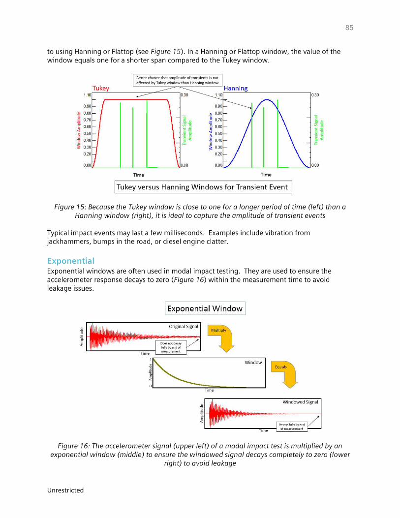
85

Unrestricted

to using Hanning or Flattop (see Figure 15). In a Hanning or Flattop window, the value of the window equals one for a shorter span compared to the Tukey window.

Figure 15: Because the Tukey window is close to one for a longer period of time (left) than a Hanning window (right), it is ideal to capture the amplitude of transient events

Typical impact events may last a few milliseconds. Examples include vibration from jackhammers, bumps in the road, or diesel engine clatter.

Exponential Exponential windows are often used in modal impact testing. They are used to ensure the accelerometer response decays to zero (Figure 16) within the measurement time to avoid leakage issues.

Figure 16: The accelerometer signal (upper left) of a modal impact test is multiplied by an exponential window (middle) to ensure the windowed signal decays completely to zero (lower

right) to avoid leakage

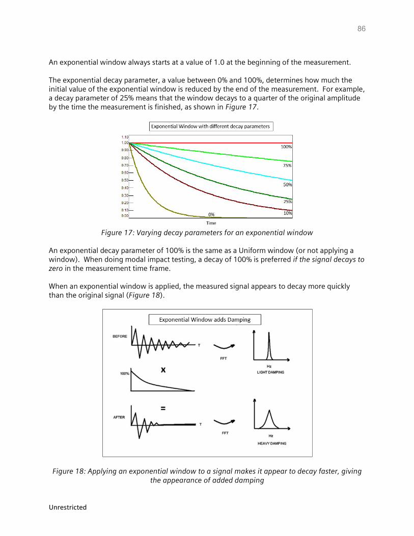
86

Unrestricted

An exponential window always starts at a value of 1.0 at the beginning of the measurement. The exponential decay parameter, a value between 0% and 100%, determines how much the initial value of the exponential window is reduced by the end of the measurement. For example, a decay parameter of 25% means that the window decays to a quarter of the original amplitude by the time the measurement is finished, as shown in Figure 17.

Figure 17: Varying decay parameters for an exponential window

An exponential decay parameter of 100% is the same as a Uniform window (or not applying a window). When doing modal impact testing, a decay of 100% is preferred if the signal decays to zero in the measurement time frame. When an exponential window is applied, the measured signal appears to decay more quickly than the original signal (Figure 18).

Figure 18: Applying an exponential window to a signal makes it appear to decay faster, giving the appearance of added damping

87

Unrestricted

By decaying faster, artificial damping is added to the resulting measurement. Using the exponential decay parameter recorded in the data, modal curve fitters in Simcenter Testlab can remove the effects and report the correct modal damping values.

Conclusion Selecting a window to match the measurement data circumstances is important to get accurate and useful data. For example, a Flattop window is ideal for performing a calibration, while an Exponential window is not appropriate. Hopefully this article provides useful guidance on which windows to use and under what circumstances.

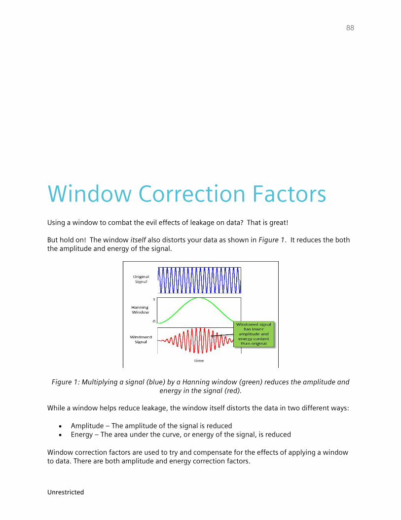
88

Unrestricted

Window Correction Factors Using a window to combat the evil effects of leakage on data? That is great! But hold on! The window itself also distorts your data as shown in Figure 1. It reduces the both the amplitude and energy of the signal.

Figure 1: Multiplying a signal (blue) by a Hanning window (green) reduces the amplitude and energy in the signal (red).

While a window helps reduce leakage, the window itself distorts the data in two different ways:

Amplitude – The amplitude of the signal is reduced Energy – The area under the curve, or energy of the signal, is reduced

Window correction factors are used to try and compensate for the effects of applying a window to data. There are both amplitude and energy correction factors.

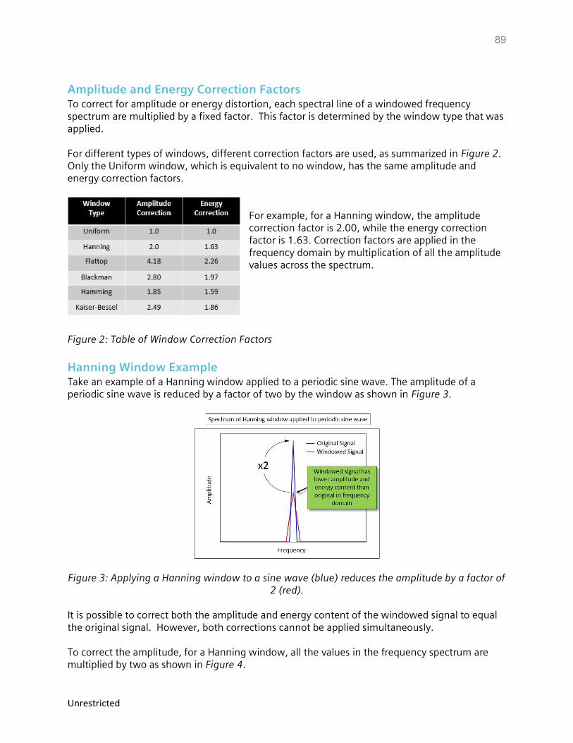
89

Unrestricted

Amplitude and Energy Correction Factors To correct for amplitude or energy distortion, each spectral line of a windowed frequency spectrum are multiplied by a fixed factor. This factor is determined by the window type that was applied. For different types of windows, different correction factors are used, as summarized in Figure 2. Only the Uniform window, which is equivalent to no window, has the same amplitude and energy correction factors.

For example, for a Hanning window, the amplitude correction factor is 2.00, while the energy correction factor is 1.63. Correction factors are applied in the frequency domain by multiplication of all the amplitude values across the spectrum.

Figure 2: Table of Window Correction Factors

Hanning Window Example Take an example of a Hanning window applied to a periodic sine wave. The amplitude of a periodic sine wave is reduced by a factor of two by the window as shown in Figure 3.

Figure 3: Applying a Hanning window to a sine wave (blue) reduces the amplitude by a factor of 2 (red).

It is possible to correct both the amplitude and energy content of the windowed signal to equal the original signal. However, both corrections cannot be applied simultaneously. To correct the amplitude, for a Hanning window, all the values in the frequency spectrum are multiplied by two as shown in Figure 4.

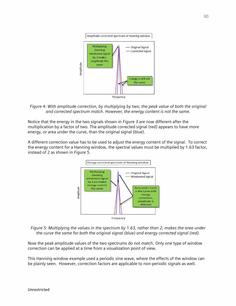
90

Unrestricted

Figure 4: With amplitude correction, by multiplying by two, the peak value of both the original and corrected spectrum match. However, the energy content is not the same.

Notice that the energy in the two signals shown in Figure 3 are now different after the multiplication by a factor of two. The amplitude corrected signal (red) appears to have more energy, or area under the curve, than the original signal (blue). A different correction value has to be used to adjust the energy content of the signal. To correct the energy content for a Hanning window, the spectral values must be multiplied by 1.63 factor, instead of 2 as shown in Figure 5.

Figure 5: Multiplying the values in the spectrum by 1.63, rather than 2, makes the area under the curve the same for both the original signal (blue) and energy corrected signal (red).

Now the peak amplitude values of the two spectrums do not match. Only one type of window correction can be applied at a time from a visualization point of view. This Hanning window example used a periodic sine wave, where the effects of the window can be plainly seen. However, correction factors are applicable to non-periodic signals as well.

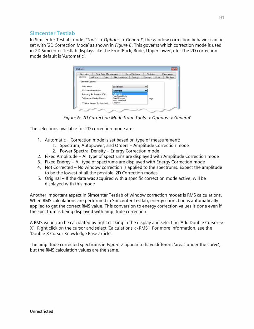
91

Unrestricted

Simcenter Testlab In Simcenter Testlab, under ‘Tools -> Options -> General’, the window correction behavior can be set with ‘2D Correction Mode’ as shown in Figure 6. This governs which correction mode is used in 2D Simcenter Testlab displays like the FrontBack, Bode, UpperLower, etc. The 2D correction mode default is ‘Automatic’.

Figure 6: 2D Correction Mode from ‘Tools -> Options -> General’

The selections available for 2D correction mode are:

1. Automatic – Correction mode is set based on type of measurement: 1. Spectrum, Autopower, and Orders – Amplitude Correction mode 2. Power Spectral Density – Energy Correction mode

2. Fixed Amplitude – All type of spectrums are displayed with Amplitude Correction mode 3. Fixed Energy – All type of spectrums are displayed with Energy Correction mode 4. Not Corrected – No window correction is applied to the spectrums. Expect the amplitude

to be the lowest of all the possible ‘2D Correction modes’ 5. Original – If the data was acquired with a specific correction mode active, will be

displayed with this mode

Another important aspect in Simcenter Testlab of window correction modes is RMS calculations. When RMS calculations are performed in Simcenter Testlab, energy correction is automatically applied to get the correct RMS value. This conversion to energy correction values is done even if the spectrum is being displayed with amplitude correction. A RMS value can be calculated by right clicking in the display and selecting ‘Add Double Cursor -> X’. Right click on the cursor and select ‘Calculations -> RMS’. For more information, see the ‘Double X Cursor Knowledge Base article’. The amplitude corrected spectrums in Figure 7 appear to have different ‘areas under the curve’, but the RMS calculation values are the same.

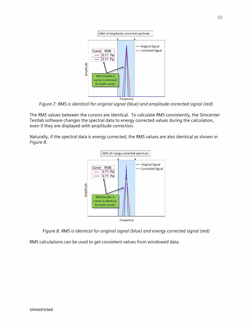
92

Unrestricted

Figure 7: RMS is identical for original signal (blue) and amplitude corrected signal (red)

The RMS values between the cursors are identical. To calculate RMS consistently, the Simcenter Testlab software changes the spectral data to energy corrected values during the calculation, even if they are displayed with amplitude correction. Naturally, if the spectral data is energy corrected, the RMS values are also identical as shown in Figure 8.

Figure 8: RMS is identical for original signal (blue) and energy corrected signal (red) RMS calculations can be used to get consistent values from windowed data.

93

Unrestricted

Conclusions A summary of the main points in this article:

Applying a window to a signal reduces the amplitude and energy of the signal In the frequency domain, either the amplitude or energy can be corrected by multiplying

by the appropriate correction factor The RMS calculation in Simcenter Testlab will always use energy corrected values, even if

amplitude corrected values are being displayed, to get the correct RMS value

Note: In this article, a periodic sine wave was used as an example. Window corrections are equally applicable to non-periodic signals.

94

Unrestricted

Root Mean Square (RMS) and Overall Level There are several different ways that the term Root Mean Square (RMS) is used. This article will go over the following:

RMS Amplitude Format: How the equivalent energy of a sine wave is expressed in a spectrum

RMS of a Spectrum: A representation of the overall energy in a spectrum – often called the overall level

Tracked RMS / Tracked Overall Level: Tracking the RMS of each average against a tracking parameter to see how the energy content changes

RMS in Simcenter Testlab

RMS Amplitude Format Amplitude formats describe how the amplitude of a sine wave is expressed in a spectrum. The RMS amplitude format is valuable because it indicates the equivalent steady state energy value of an oscillating signal. For example, a sine wave (like a pressure wave) oscillates above and below zero Pascal. The average value of the wave is zero. This is not a good representation of the effective energy of the wave. To get a better understanding of the equivalent steady state value, the RMS is used.

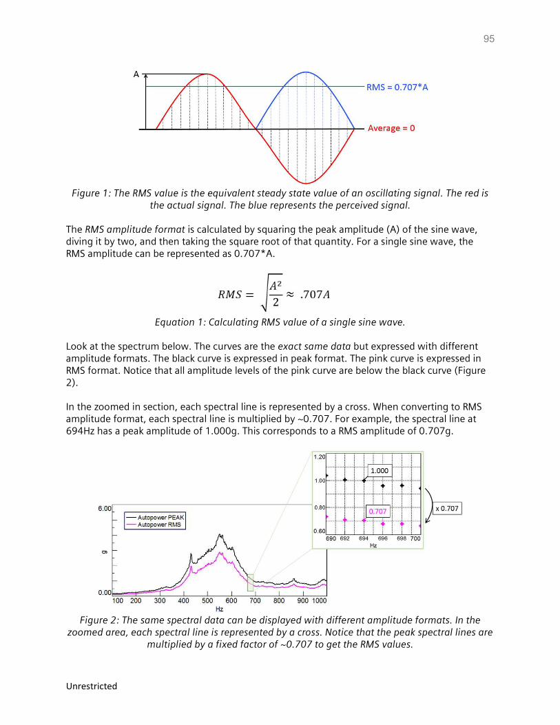
95

Unrestricted

Figure 1: The RMS value is the equivalent steady state value of an oscillating signal. The red is

the actual signal. The blue represents the perceived signal. The RMS amplitude format is calculated by squaring the peak amplitude (A) of the sine wave, diving it by two, and then taking the square root of that quantity. For a single sine wave, the RMS amplitude can be represented as 0.707*A.

Equation 1: Calculating RMS value of a single sine wave.

Look at the spectrum below. The curves are the exact same data but expressed with different amplitude formats. The black curve is expressed in peak format. The pink curve is expressed in RMS format. Notice that all amplitude levels of the pink curve are below the black curve (Figure 2). In the zoomed in section, each spectral line is represented by a cross. When converting to RMS amplitude format, each spectral line is multiplied by ~0.707. For example, the spectral line at 694Hz has a peak amplitude of 1.000g. This corresponds to a RMS amplitude of 0.707g.

Figure 2: The same spectral data can be displayed with different amplitude formats. In the

zoomed area, each spectral line is represented by a cross. Notice that the peak spectral lines are multiplied by a fixed factor of ~0.707 to get the RMS values.

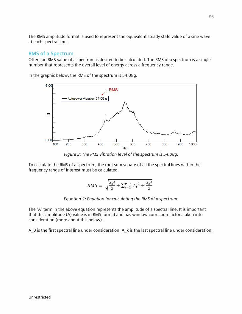
96

Unrestricted

The RMS amplitude format is used to represent the equivalent steady state value of a sine wave at each spectral line.

RMS of a Spectrum Often, an RMS value of a spectrum is desired to be calculated. The RMS of a spectrum is a single number that represents the overall level of energy across a frequency range. In the graphic below, the RMS of the spectrum is 54.08g.

Figure 3: The RMS vibration level of the spectrum is 54.08g.

To calculate the RMS of a spectrum, the root sum square of all the spectral lines within the frequency range of interest must be calculated.

Equation 2: Equation for calculating the RMS of a spectrum.

The “A” term in the above equation represents the amplitude of a spectral line. It is important that this amplitude (A) value is in RMS format and has window correction factors taken into consideration (more about this below). A_0 is the first spectral line under consideration, A_k is the last spectral line under consideration.

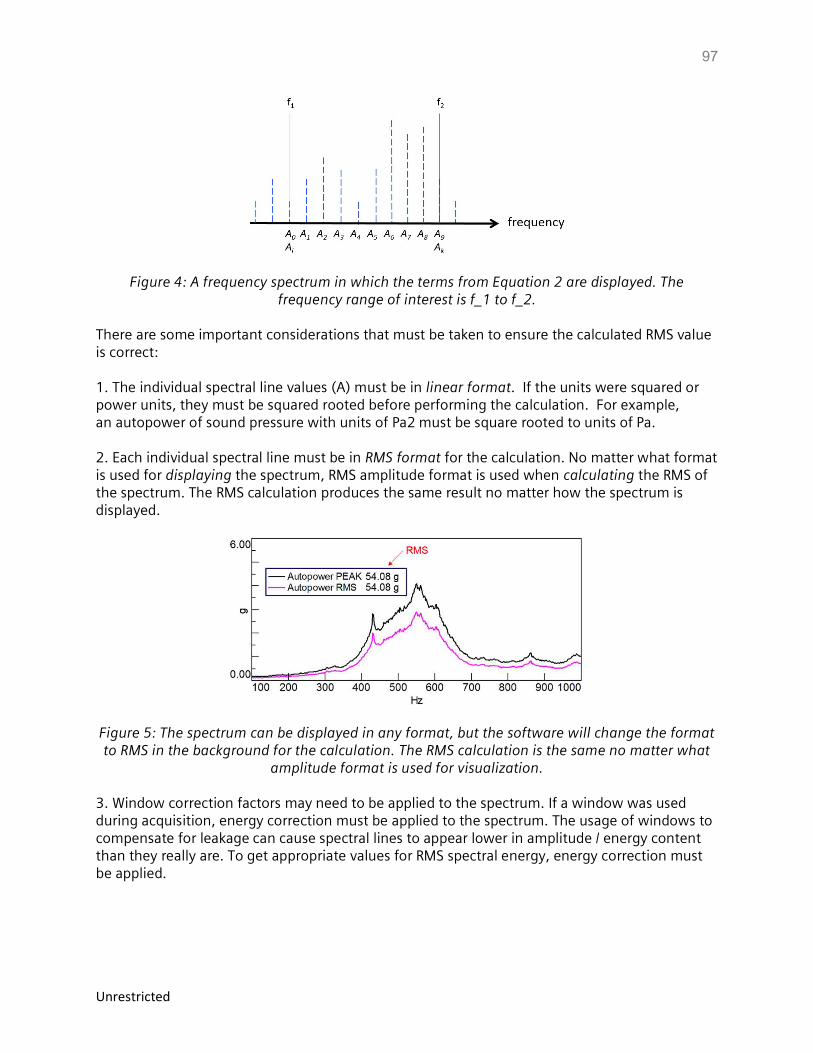
97

Unrestricted

Figure 4: A frequency spectrum in which the terms from Equation 2 are displayed. The frequency range of interest is f_1 to f_2.

There are some important considerations that must be taken to ensure the calculated RMS value is correct: 1. The individual spectral line values (A) must be in linear format. If the units were squared or power units, they must be squared rooted before performing the calculation. For example, an autopower of sound pressure with units of Pa2 must be square rooted to units of Pa. 2. Each individual spectral line must be in RMS format for the calculation. No matter what format is used for displaying the spectrum, RMS amplitude format is used when calculating the RMS of the spectrum. The RMS calculation produces the same result no matter how the spectrum is displayed.

Figure 5: The spectrum can be displayed in any format, but the software will change the format to RMS in the background for the calculation. The RMS calculation is the same no matter what

amplitude format is used for visualization.

3. Window correction factors may need to be applied to the spectrum. If a window was used during acquisition, energy correction must be applied to the spectrum. The usage of windows to compensate for leakage can cause spectral lines to appear lower in amplitude / energy content than they really are. To get appropriate values for RMS spectral energy, energy correction must be applied.

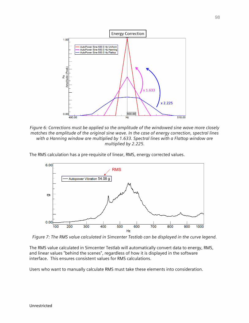
98

Unrestricted

Figure 6: Corrections must be applied so the amplitude of the windowed sine wave more closely matches the amplitude of the original sine wave. In the case of energy correction, spectral lines

with a Hanning window are multiplied by 1.633. Spectral lines with a Flattop window are multiplied by 2.225.

The RMS calculation has a pre-requisite of linear, RMS, energy corrected values.

Figure 7: The RMS value calculated in Simcenter Testlab can be displayed in the curve legend.

The RMS value calculated in Simcenter Testlab will automatically convert data to energy, RMS, and linear values "behind the scenes", regardless of how it is displayed in the software interface. This ensures consistent values for RMS calculations. Users who want to manually calculate RMS must take these elements into consideration.

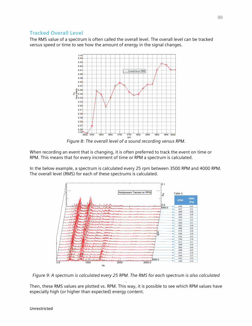
99

Unrestricted

Tracked Overall Level The RMS value of a spectrum is often called the overall level. The overall level can be tracked versus speed or time to see how the amount of energy in the signal changes.

Figure 8: The overall level of a sound recording versus RPM.

When recording an event that is changing, it is often preferred to track the event on time or RPM. This means that for every increment of time or RPM a spectrum is calculated. In the below example, a spectrum is calculated every 25 rpm between 3500 RPM and 4000 RPM. The overall level (RMS) for each of these spectrums is calculated.

Figure 9: A spectrum is calculated every 25 RPM. The RMS for each spectrum is also calculated .

Then, these RMS values are plotted vs. RPM. This way, it is possible to see which RPM values have especially high (or higher than expected) energy content.

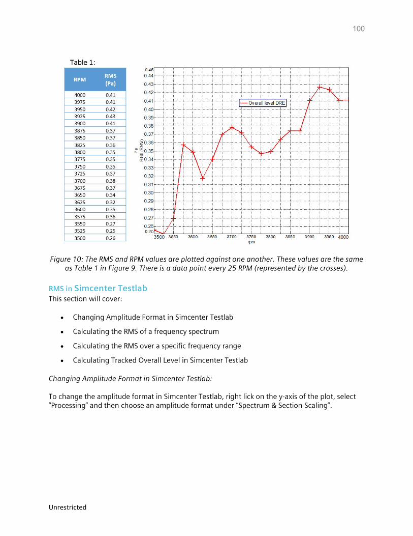
100

Unrestricted

Figure 10: The RMS and RPM values are plotted against one another. These values are the same as Table 1 in Figure 9. There is a data point every 25 RPM (represented by the crosses).

RMS in Simcenter Testlab This section will cover:

Changing Amplitude Format in Simcenter Testlab

Calculating the RMS of a frequency spectrum

Calculating the RMS over a specific frequency range

Calculating Tracked Overall Level in Simcenter Testlab

Changing Amplitude Format in Simcenter Testlab: To change the amplitude format in Simcenter Testlab, right lick on the y-axis of the plot, select “Processing” and then choose an amplitude format under “Spectrum & Section Scaling”.

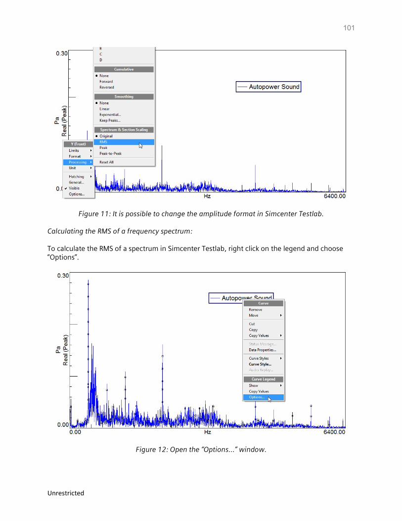
101

Unrestricted

Figure 11: It is possible to change the amplitude format in Simcenter Testlab. Calculating the RMS of a frequency spectrum: To calculate the RMS of a spectrum in Simcenter Testlab, right click on the legend and choose “Options”.

Figure 12: Open the “Options…” window.

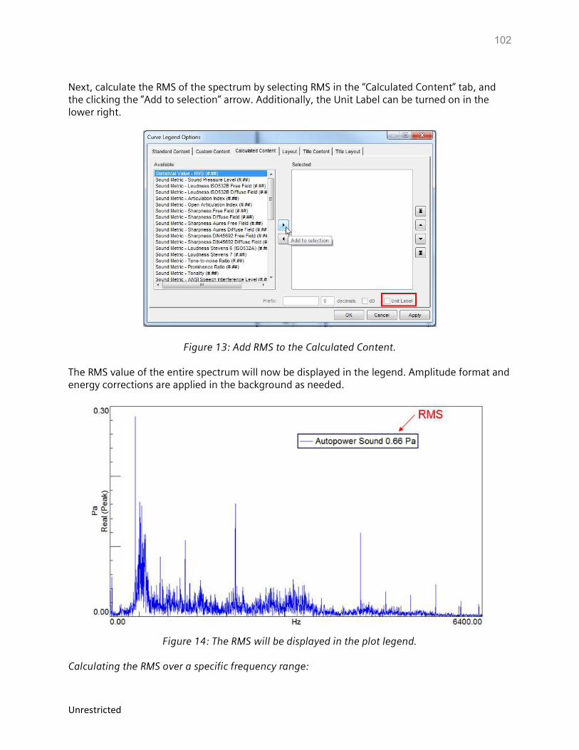
102

Unrestricted

Next, calculate the RMS of the spectrum by selecting RMS in the “Calculated Content” tab, and the clicking the “Add to selection” arrow. Additionally, the Unit Label can be turned on in the lower right.

Figure 13: Add RMS to the Calculated Content. The RMS value of the entire spectrum will now be displayed in the legend. Amplitude format and energy corrections are applied in the background as needed.

Figure 14: The RMS will be displayed in the plot legend.

Calculating the RMS over a specific frequency range:

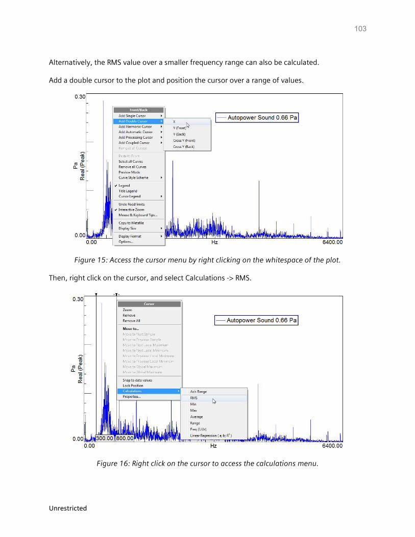
103

Unrestricted

Alternatively, the RMS value over a smaller frequency range can also be calculated. Add a double cursor to the plot and position the cursor over a range of values.

Figure 15: Access the cursor menu by right clicking on the whitespace of the plot.

Then, right click on the cursor, and select Calculations -> RMS.

Figure 16: Right click on the cursor to access the calculations menu.

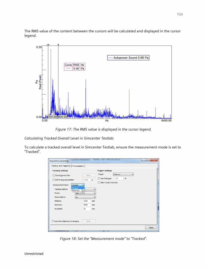
104

Unrestricted

The RMS value of the content between the cursors will be calculated and displayed in the cursor legend.

Figure 17: The RMS value is displayed in the cursor legend. Calculating Tracked Overall Level in Simcenter Testlab: To calculate a tracked overall level in Simcenter Testlab, ensure the measurement mode is set to “Tracked”.

Figure 18: Set the “Measurement mode” to “Tracked”.

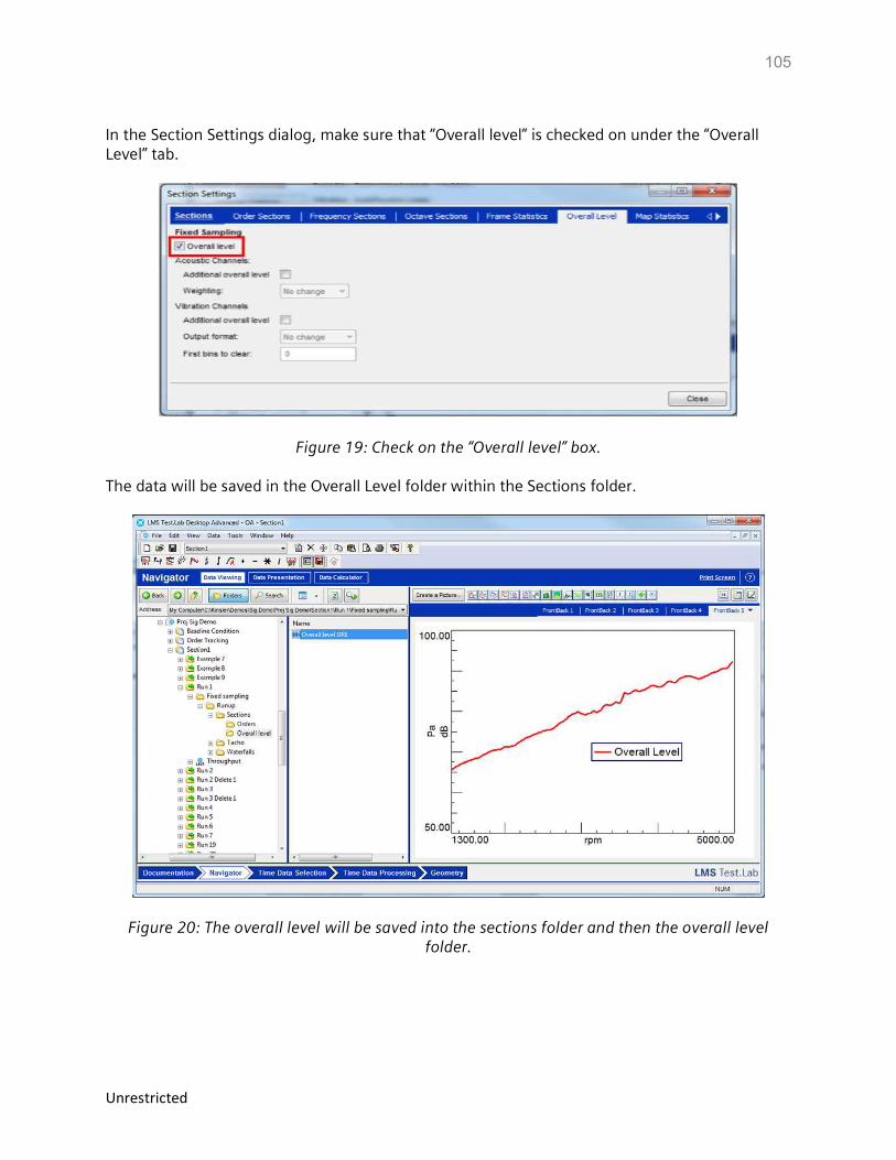
105

Unrestricted

In the Section Settings dialog, make sure that “Overall level” is checked on under the “Overall Level” tab.

Figure 19: Check on the “Overall level” box. The data will be saved in the Overall Level folder within the Sections folder.

Figure 20: The overall level will be saved into the sections folder and then the overall level folder.

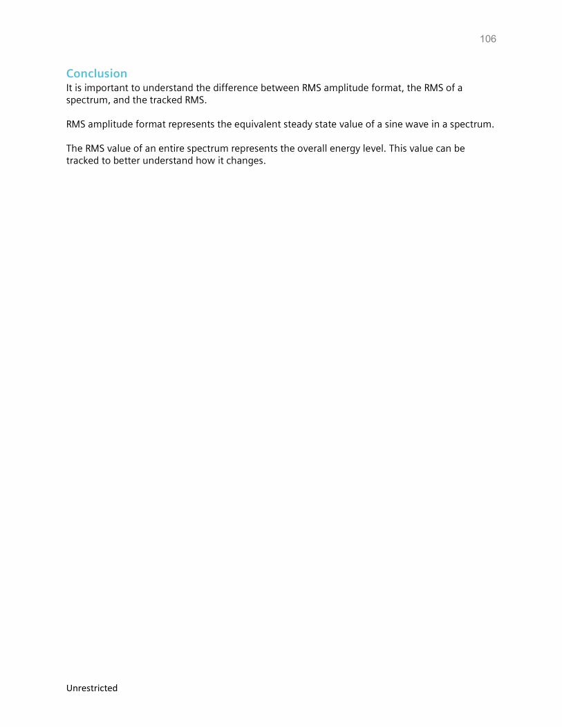
106

Unrestricted

Conclusion It is important to understand the difference between RMS amplitude format, the RMS of a spectrum, and the tracked RMS. RMS amplitude format represents the equivalent steady state value of a sine wave in a spectrum. The RMS value of an entire spectrum represents the overall energy level. This value can be tracked to better understand how it changes.

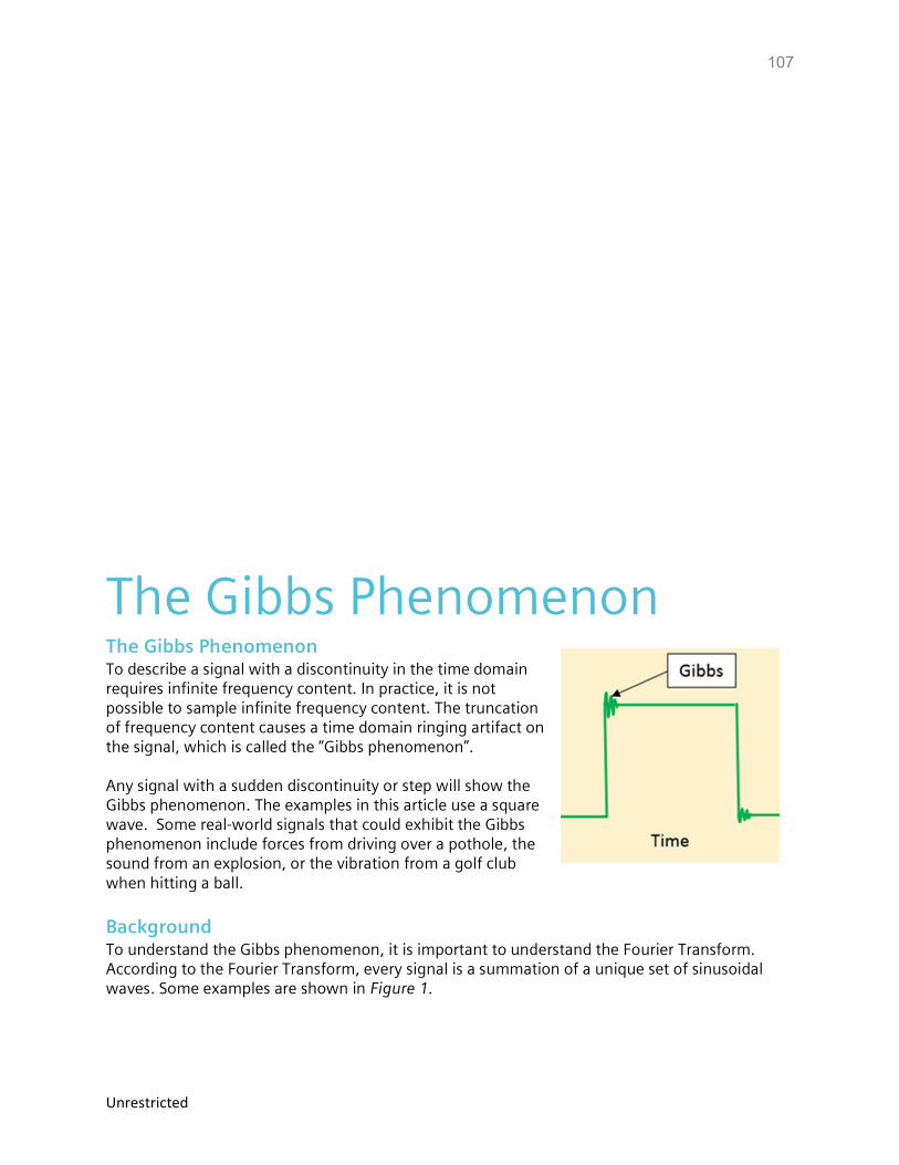
107

Unrestricted

The Gibbs Phenomenon The Gibbs Phenomenon To describe a signal with a discontinuity in the time domain requires infinite frequency content. In practice, it is not possible to sample infinite frequency content. The truncation of frequency content causes a time domain ringing artifact on the signal, which is called the “Gibbs phenomenon”. Any signal with a sudden discontinuity or step will show the Gibbs phenomenon. The examples in this article use a square wave. Some real-world signals that could exhibit the Gibbs phenomenon include forces from driving over a pothole, the sound from an explosion, or the vibration from a golf club when hitting a ball.

Background To understand the Gibbs phenomenon, it is important to understand the Fourier Transform. According to the Fourier Transform, every signal is a summation of a unique set of sinusoidal waves. Some examples are shown in Figure 1.

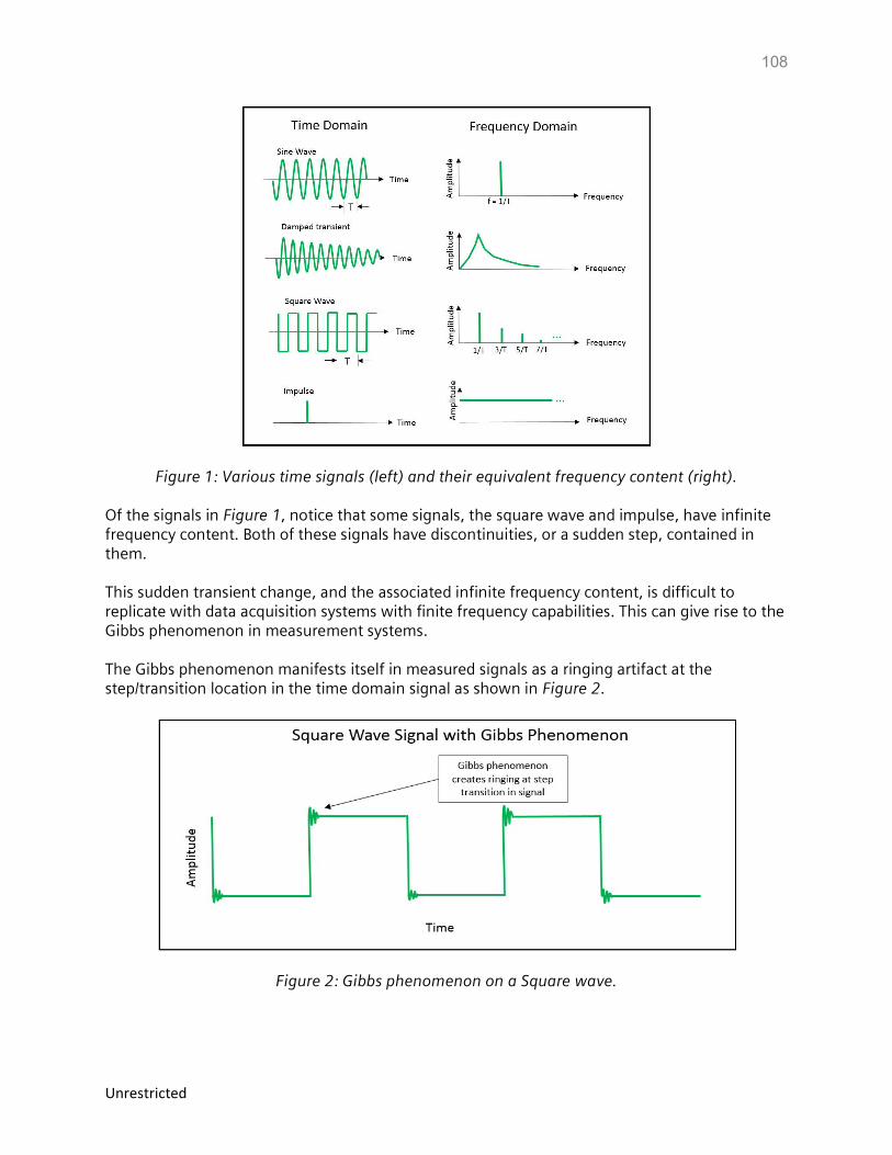
108

Unrestricted

Figure 1: Various time signals (left) and their equivalent frequency content (right). Of the signals in Figure 1, notice that some signals, the square wave and impulse, have infinite frequency content. Both of these signals have discontinuities, or a sudden step, contained in them. This sudden transient change, and the associated infinite frequency content, is difficult to replicate with data acquisition systems with finite frequency capabilities. This can give rise to the Gibbs phenomenon in measurement systems. The Gibbs phenomenon manifests itself in measured signals as a ringing artifact at the step/transition location in the time domain signal as shown in Figure 2.

Figure 2: Gibbs phenomenon on a Square wave.

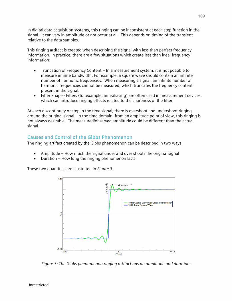
109

Unrestricted

In digital data acquisition systems, this ringing can be inconsistent at each step function in the signal. It can vary in amplitude or not occur at all. This depends on timing of the transient relative to the data samples. This ringing artifact is created when describing the signal with less than perfect frequency information. In practice, there are a few situations which create less than ideal frequency information:

Truncation of Frequency Content – In a measurement system, it is not possible to measure infinite bandwidth. For example, a square wave should contain an infinite number of harmonic frequencies. When measuring a signal, an infinite number of harmonic frequencies cannot be measured, which truncates the frequency content present in the signal.

Filter Shape - Filters (for example, anti-aliasing) are often used in measurement devices, which can introduce ringing effects related to the sharpness of the filter.

At each discontinuity or step in the time signal, there is overshoot and undershoot ringing around the original signal. In the time domain, from an amplitude point of view, this ringing is not always desirable. The measured/observed amplitude could be different than the actual signal.

Causes and Control of the Gibbs Phenomenon The ringing artifact created by the Gibbs phenomenon can be described in two ways:

Amplitude – How much the signal under and over shoots the original signal Duration – How long the ringing phenomenon lasts

These two quantities are illustrated in Figure 3.

Figure 3: The Gibbs phenomenon ringing artifact has an amplitude and duration.

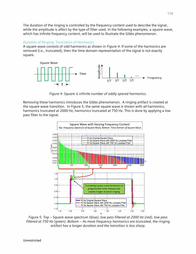
110

Unrestricted

The duration of the ringing is controlled by the frequency content used to describe the signal, while the amplitude is affect by the type of filter used. In the following examples, a square wave, which has infinite frequency content, will be used to illustrate the Gibbs phenomenon. Duration of Ringing: Truncation of Harmonics A square wave consists of odd harmonics as shown in Figure 4. If some of the harmonics are removed (i.e., truncated), then the time domain representation of the signal is not exactly square.

Figure 4: Square is infinite number of oddly spaced harmonics. Removing these harmonics introduces the Gibbs phenomenon. A ringing artifact is created at the square wave transition. In Figure 5, the same square wave is shown with all harmonics, harmonics truncated at 2000 Hz, harmonics truncated at 750 Hz. This is done by applying a low pass filter to the signal.

Figure 5: Top – Square wave spectrum (blue), low pass filtered at 2000 Hz (red), low pass

filtered at 750 Hz (green). Bottom – As more frequency harmonics are truncated, the ringing artifact has a longer duration and the transition is less sharp.

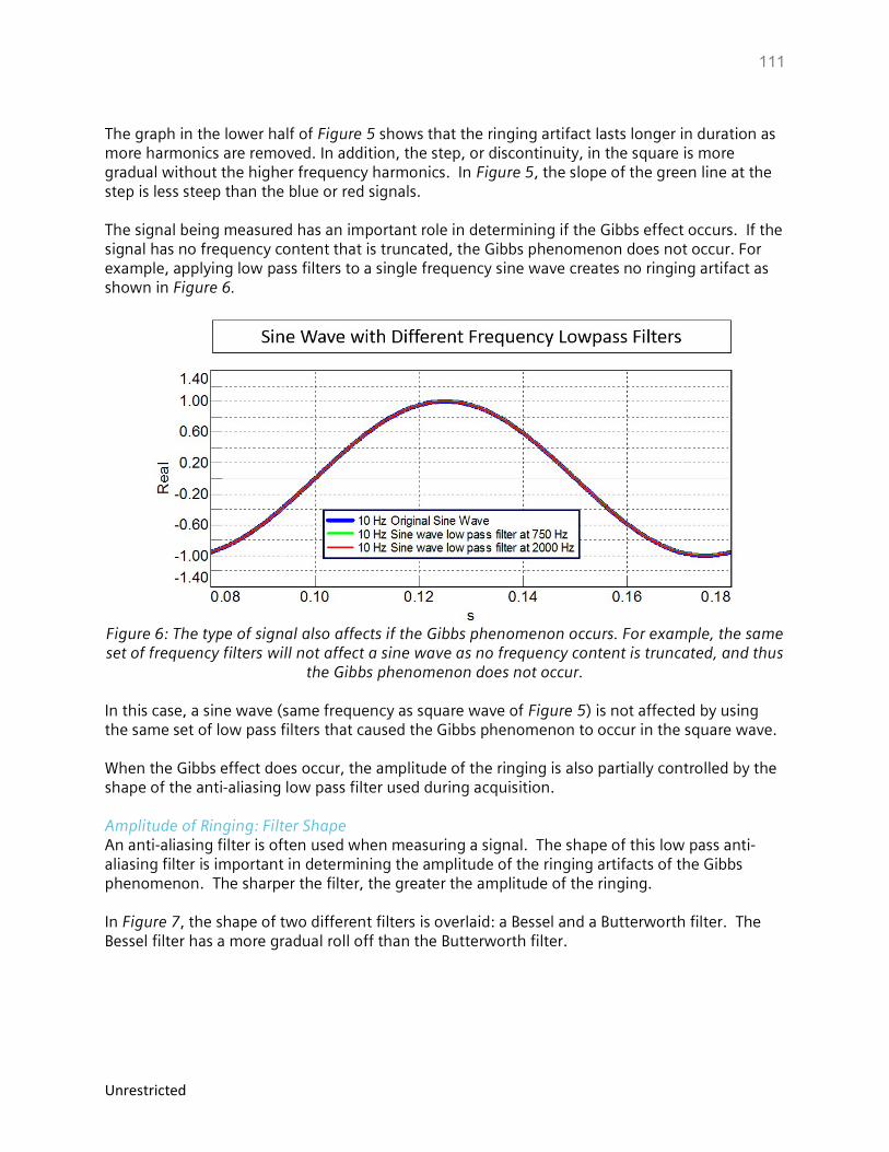
111

Unrestricted

The graph in the lower half of Figure 5 shows that the ringing artifact lasts longer in duration as more harmonics are removed. In addition, the step, or discontinuity, in the square is more gradual without the higher frequency harmonics. In Figure 5, the slope of the green line at the step is less steep than the blue or red signals. The signal being measured has an important role in determining if the Gibbs effect occurs. If the signal has no frequency content that is truncated, the Gibbs phenomenon does not occur. For example, applying low pass filters to a single frequency sine wave creates no ringing artifact as shown in Figure 6.

Figure 6: The type of signal also affects if the Gibbs phenomenon occurs. For example, the same set of frequency filters will not affect a sine wave as no frequency content is truncated, and thus

the Gibbs phenomenon does not occur. In this case, a sine wave (same frequency as square wave of Figure 5) is not affected by using the same set of low pass filters that caused the Gibbs phenomenon to occur in the square wave. When the Gibbs effect does occur, the amplitude of the ringing is also partially controlled by the shape of the anti-aliasing low pass filter used during acquisition. Amplitude of Ringing: Filter Shape An anti-aliasing filter is often used when measuring a signal. The shape of this low pass anti-aliasing filter is important in determining the amplitude of the ringing artifacts of the Gibbs phenomenon. The sharper the filter, the greater the amplitude of the ringing. In Figure 7, the shape of two different filters is overlaid: a Bessel and a Butterworth filter. The Bessel filter has a more gradual roll off than the Butterworth filter.

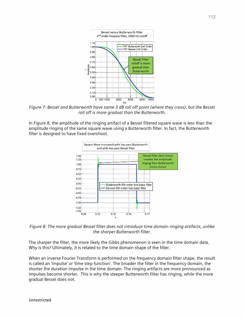
112

Unrestricted

Figure 7: Bessel and Butterworth have same 3 dB roll off point (where they cross), but the Bessel

roll off is more gradual than the Butterworth.

In Figure 8, the amplitude of the ringing artifact of a Bessel filtered square wave is less than the amplitude ringing of the same square wave using a Butterworth filter. In fact, the Butterworth filter is designed to have fixed overshoot.

Figure 8: The more gradual Bessel filter does not introduce time domain ringing artifacts, unlike the sharper Butterworth filter.

The sharper the filter, the more likely the Gibbs phenomenon is seen in the time domain data. Why is this? Ultimately, it is related to the time domain shape of the filter. When an inverse Fourier Transform is performed on the frequency domain filter shape, the result is called an ‘impulse’ or ‘time step function’. The broader the filter in the frequency domain, the shorter the duration impulse in the time domain. The ringing artifacts are more pronounced as impulses become shorter. This is why the steeper Butterworth filter has ringing, while the more gradual Bessel does not.

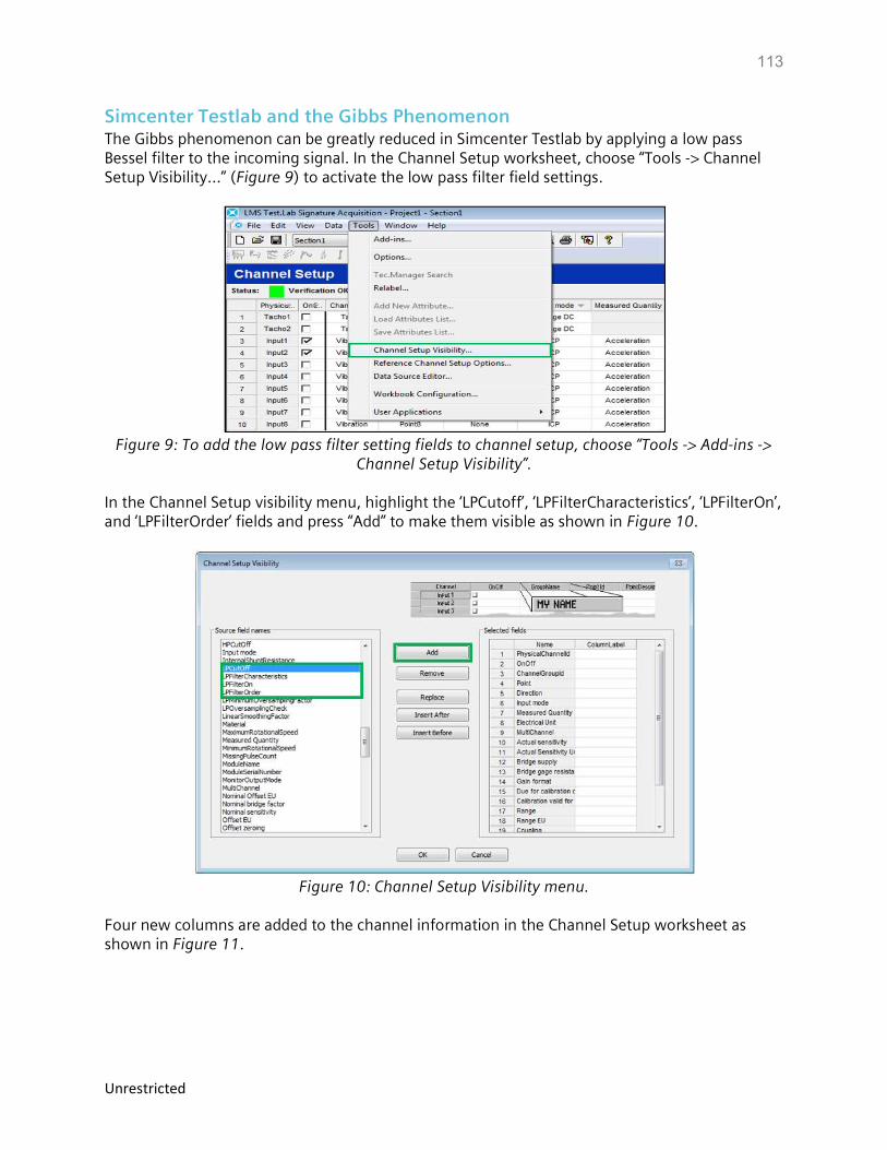
113

Unrestricted

Simcenter Testlab and the Gibbs Phenomenon The Gibbs phenomenon can be greatly reduced in Simcenter Testlab by applying a low pass Bessel filter to the incoming signal. In the Channel Setup worksheet, choose “Tools -> Channel Setup Visibility…” (Figure 9) to activate the low pass filter field settings.

Figure 9: To add the low pass filter setting fields to channel setup, choose “Tools -> Add-ins ->

Channel Setup Visibility”.

In the Channel Setup visibility menu, highlight the ‘LPCutoff’, ‘LPFilterCharacteristics’, ‘LPFilterOn’, and ‘LPFilterOrder’ fields and press “Add” to make them visible as shown in Figure 10.

Figure 10: Channel Setup Visibility menu.

Four new columns are added to the channel information in the Channel Setup worksheet as shown in Figure 11.

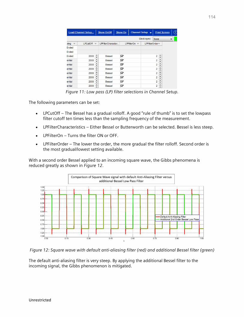
114

Unrestricted

Figure 11: Low pass (LP) filter selections in Channel Setup.

The following parameters can be set:

LPCutOff – The Bessel has a gradual rolloff. A good “rule of thumb” is to set the lowpass filter cutoff ten times less than the sampling frequency of the measurement.

LPFilterCharacteristics – Either Bessel or Butterworth can be selected. Bessel is less steep.

LPFilterOn – Turns the filter ON or OFF.

LPFilterOrder – The lower the order, the more gradual the filter rolloff. Second order is the most gradual/lowest setting available.

With a second order Bessel applied to an incoming square wave, the Gibbs phenomena is reduced greatly as shown in Figure 12.

Figure 12: Square wave with default anti-aliasing filter (red) and additional Bessel filter (green) The default anti-aliasing filter is very steep. By applying the additional Bessel filter to the incoming signal, the Gibbs phenomenon is mitigated.

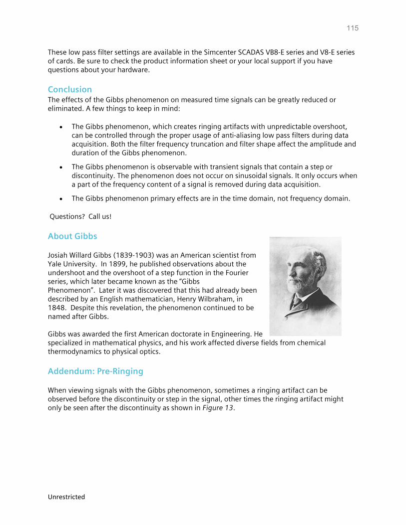
115

Unrestricted

These low pass filter settings are available in the Simcenter SCADAS VB8-E series and V8-E series of cards. Be sure to check the product information sheet or your local support if you have questions about your hardware.

Conclusion The effects of the Gibbs phenomenon on measured time signals can be greatly reduced or eliminated. A few things to keep in mind:

The Gibbs phenomenon, which creates ringing artifacts with unpredictable overshoot, can be controlled through the proper usage of anti-aliasing low pass filters during data acquisition. Both the filter frequency truncation and filter shape affect the amplitude and duration of the Gibbs phenomenon.

The Gibbs phenomenon is observable with transient signals that contain a step or discontinuity. The phenomenon does not occur on sinusoidal signals. It only occurs when a part of the frequency content of a signal is removed during data acquisition.

The Gibbs phenomenon primary effects are in the time domain, not frequency domain.

Questions? Call us!

About Gibbs Josiah Willard Gibbs (1839-1903) was an American scientist from Yale University. In 1899, he published observations about the undershoot and the overshoot of a step function in the Fourier series, which later became known as the “Gibbs Phenomenon”. Later it was discovered that this had already been described by an English mathematician, Henry Wilbraham, in 1848. Despite this revelation, the phenomenon continued to be named after Gibbs. Gibbs was awarded the first American doctorate in Engineering. He specialized in mathematical physics, and his work affected diverse fields from chemical thermodynamics to physical optics.

Addendum: Pre-Ringing When viewing signals with the Gibbs phenomenon, sometimes a ringing artifact can be observed before the discontinuity or step in the signal, other times the ringing artifact might only be seen after the discontinuity as shown in Figure 13.

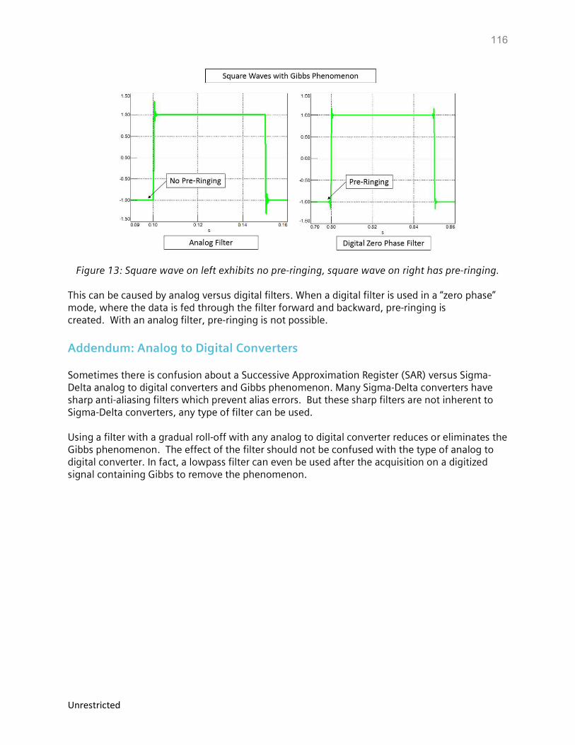
116

Unrestricted

Figure 13: Square wave on left exhibits no pre-ringing, square wave on right has pre-ringing.

This can be caused by analog versus digital filters. When a digital filter is used in a “zero phase” mode, where the data is fed through the filter forward and backward, pre-ringing is created. With an analog filter, pre-ringing is not possible.

Addendum: Analog to Digital Converters Sometimes there is confusion about a Successive Approximation Register (SAR) versus Sigma-Delta analog to digital converters and Gibbs phenomenon. Many Sigma-Delta converters have sharp anti-aliasing filters which prevent alias errors. But these sharp filters are not inherent to Sigma-Delta converters, any type of filter can be used. Using a filter with a gradual roll-off with any analog to digital converter reduces or eliminates the Gibbs phenomenon. The effect of the filter should not be confused with the type of analog to digital converter. In fact, a lowpass filter can even be used after the acquisition on a digitized signal containing Gibbs to remove the phenomenon.

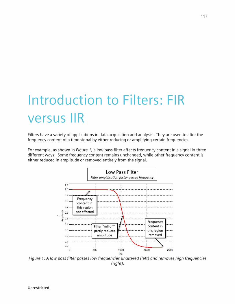
117

Unrestricted

Introduction to Filters: FIR versus IIR Filters have a variety of applications in data acquisition and analysis. They are used to alter the frequency content of a time signal by either reducing or amplifying certain frequencies. For example, as shown in Figure 1, a low pass filter affects frequency content in a signal in three different ways: Some frequency content remains unchanged, while other frequency content is either reduced in amplitude or removed entirely from the signal.

Figure 1: A low pass filter passes low frequencies unaltered (left) and removes high frequencies

(right).

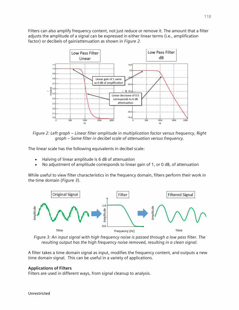
118

Unrestricted

Filters can also amplify frequency content, not just reduce or remove it. The amount that a filter adjusts the amplitude of a signal can be expressed in either linear terms (i.e., amplification factor) or decibels of gain/attenuation as shown in Figure 2.

Figure 2: Left graph – Linear filter amplitude in multiplication factor versus frequency, Right graph – Same filter in decibel scale of attenuation versus frequency.

The linear scale has the following equivalents in decibel scale:

Halving of linear amplitude is 6 dB of attenuation No adjustment of amplitude corresponds to linear gain of 1, or 0 dB, of attenuation

While useful to view filter characteristics in the frequency domain, filters perform their work in the time domain (Figure 3).

Figure 3: An input signal with high frequency noise is passed through a low pass filter. The resulting output has the high frequency noise removed, resulting in a clean signal.

A filter takes a time domain signal as input, modifies the frequency content, and outputs a new time domain signal. This can be useful in a variety of applications. Applications of Filters Filters are used in different ways, from signal cleanup to analysis.

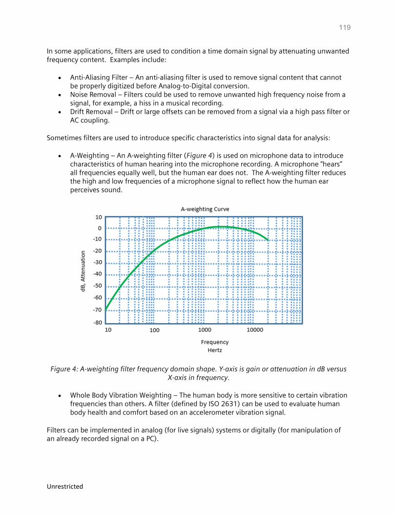
119

Unrestricted

In some applications, filters are used to condition a time domain signal by attenuating unwanted frequency content. Examples include:

Anti-Aliasing Filter – An anti-aliasing filter is used to remove signal content that cannot be properly digitized before Analog-to-Digital conversion.

Noise Removal – Filters could be used to remove unwanted high frequency noise from a signal, for example, a hiss in a musical recording.

Drift Removal – Drift or large offsets can be removed from a signal via a high pass filter or AC coupling.

Sometimes filters are used to introduce specific characteristics into signal data for analysis:

A-Weighting – An A-weighting filter (Figure 4) is used on microphone data to introduce characteristics of human hearing into the microphone recording. A microphone “hears” all frequencies equally well, but the human ear does not. The A-weighting filter reduces the high and low frequencies of a microphone signal to reflect how the human ear perceives sound.

Figure 4: A-weighting filter frequency domain shape. Y-axis is gain or attenuation in dB versus X-axis in frequency.

Whole Body Vibration Weighting – The human body is more sensitive to certain vibration frequencies than others. A filter (defined by ISO 2631) can be used to evaluate human body health and comfort based on an accelerometer vibration signal.

Filters can be implemented in analog (for live signals) systems or digitally (for manipulation of an already recorded signal on a PC).

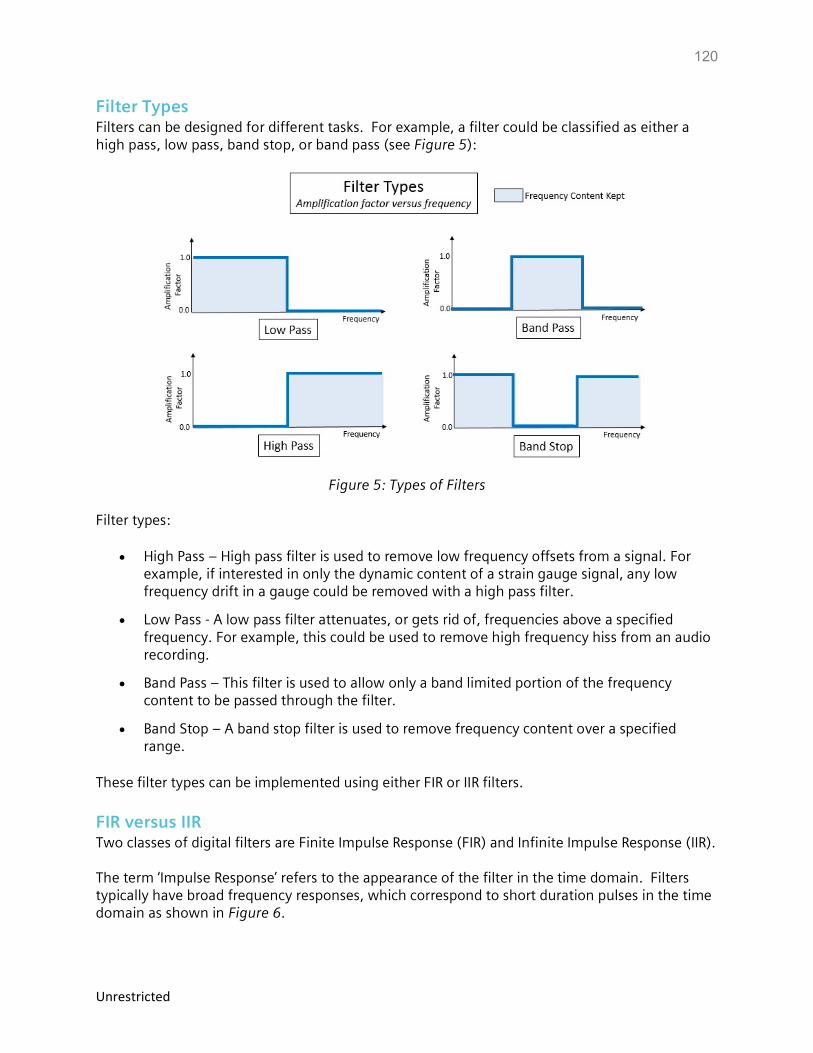
120

Unrestricted

Filter Types Filters can be designed for different tasks. For example, a filter could be classified as either a high pass, low pass, band stop, or band pass (see Figure 5):

Figure 5: Types of Filters Filter types:

High Pass – High pass filter is used to remove low frequency offsets from a signal. For example, if interested in only the dynamic content of a strain gauge signal, any low frequency drift in a gauge could be removed with a high pass filter.

Low Pass - A low pass filter attenuates, or gets rid of, frequencies above a specified frequency. For example, this could be used to remove high frequency hiss from an audio recording.

Band Pass – This filter is used to allow only a band limited portion of the frequency content to be passed through the filter.

Band Stop – A band stop filter is used to remove frequency content over a specified range.

These filter types can be implemented using either FIR or IIR filters.

FIR versus IIR Two classes of digital filters are Finite Impulse Response (FIR) and Infinite Impulse Response (IIR). The term ‘Impulse Response’ refers to the appearance of the filter in the time domain. Filters typically have broad frequency responses, which correspond to short duration pulses in the time domain as shown in Figure 6.

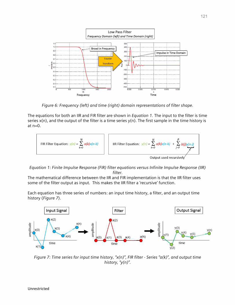
121

Unrestricted

Figure 6: Frequency (left) and time (right) domain representations of filter shape. The equations for both an IIR and FIR filter are shown in Equation 1. The input to the filter is time series x(n), and the output of the filter is a time series y(n). The first sample in the time history is at n=0.

Equation 1: Finite Impulse Response (FIR) filter equations versus Infinite Impulse Response (IIR) filter.

The mathematical difference between the IIR and FIR implementation is that the IIR filter uses some of the filter output as input. This makes the IIR filter a ‘recursive’ function. Each equation has three series of numbers: an input time history, a filter, and an output time history (Figure 7).

Figure 7: Time series for input time history, “x(n)”, FIR filter - Series “a(k)”, and output time history, “y(n)”.

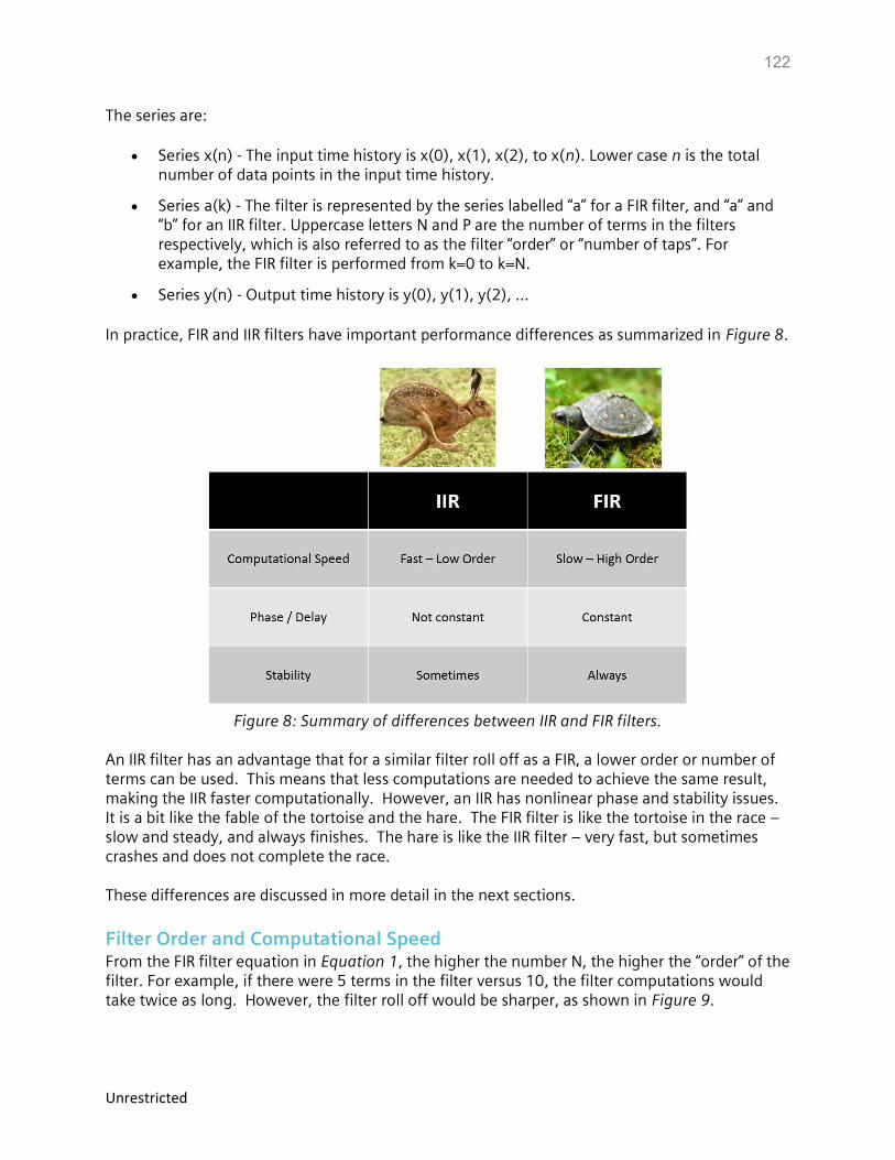
122

Unrestricted

The series are:

Series x(n) - The input time history is x(0), x(1), x(2), to x(n). Lower case n is the total number of data points in the input time history.

Series a(k) - The filter is represented by the series labelled “a” for a FIR filter, and “a” and “b” for an IIR filter. Uppercase letters N and P are the number of terms in the filters respectively, which is also referred to as the filter “order” or “number of taps”. For example, the FIR filter is performed from k=0 to k=N.

Series y(n) - Output time history is y(0), y(1), y(2), …

In practice, FIR and IIR filters have important performance differences as summarized in Figure 8.

Figure 8: Summary of differences between IIR and FIR filters.

An IIR filter has an advantage that for a similar filter roll off as a FIR, a lower order or number of terms can be used. This means that less computations are needed to achieve the same result, making the IIR faster computationally. However, an IIR has nonlinear phase and stability issues. It is a bit like the fable of the tortoise and the hare. The FIR filter is like the tortoise in the race – slow and steady, and always finishes. The hare is like the IIR filter – very fast, but sometimes crashes and does not complete the race. These differences are discussed in more detail in the next sections.

Filter Order and Computational Speed From the FIR filter equation in Equation 1, the higher the number N, the higher the “order” of the filter. For example, if there were 5 terms in the filter versus 10, the filter computations would take twice as long. However, the filter roll off would be sharper, as shown in Figure 9.

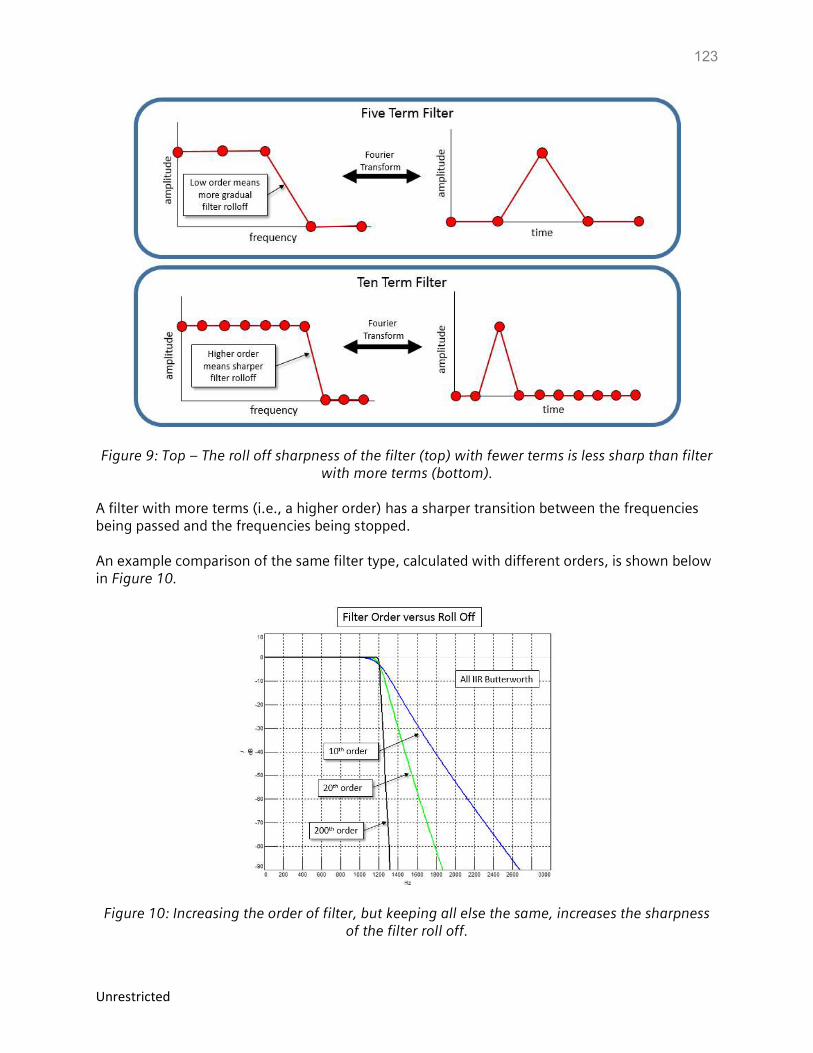
123

Unrestricted

Figure 9: Top – The roll off sharpness of the filter (top) with fewer terms is less sharp than filter with more terms (bottom).

A filter with more terms (i.e., a higher order) has a sharper transition between the frequencies being passed and the frequencies being stopped. An example comparison of the same filter type, calculated with different orders, is shown below in Figure 10.

Figure 10: Increasing the order of filter, but keeping all else the same, increases the sharpness of the filter roll off.

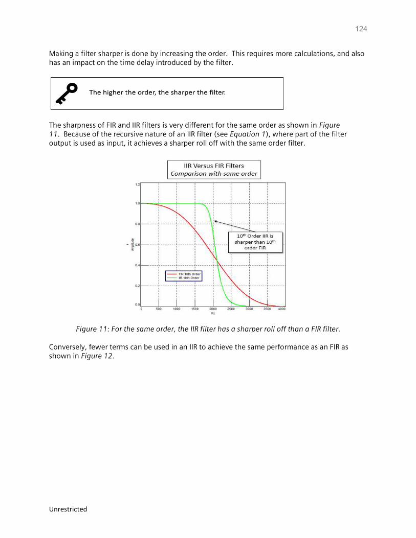
124

Unrestricted

Making a filter sharper is done by increasing the order. This requires more calculations, and also has an impact on the time delay introduced by the filter.

The sharpness of FIR and IIR filters is very different for the same order as shown in Figure 11. Because of the recursive nature of an IIR filter (see Equation 1), where part of the filter output is used as input, it achieves a sharper roll off with the same order filter.

Figure 11: For the same order, the IIR filter has a sharper roll off than a FIR filter.

Conversely, fewer terms can be used in an IIR to achieve the same performance as an FIR as shown in Figure 12.

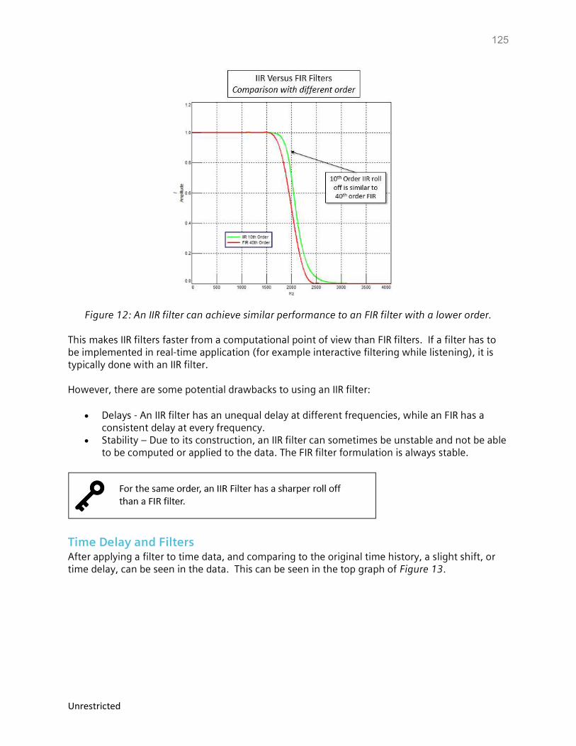
125

Unrestricted

Figure 12: An IIR filter can achieve similar performance to an FIR filter with a lower order.

This makes IIR filters faster from a computational point of view than FIR filters. If a filter has to be implemented in real-time application (for example interactive filtering while listening), it is typically done with an IIR filter. However, there are some potential drawbacks to using an IIR filter:

Delays - An IIR filter has an unequal delay at different frequencies, while an FIR has a consistent delay at every frequency.

Stability – Due to its construction, an IIR filter can sometimes be unstable and not be able to be computed or applied to the data. The FIR filter formulation is always stable.

Time Delay and Filters After applying a filter to time data, and comparing to the original time history, a slight shift, or time delay, can be seen in the data. This can be seen in the top graph of Figure 13.

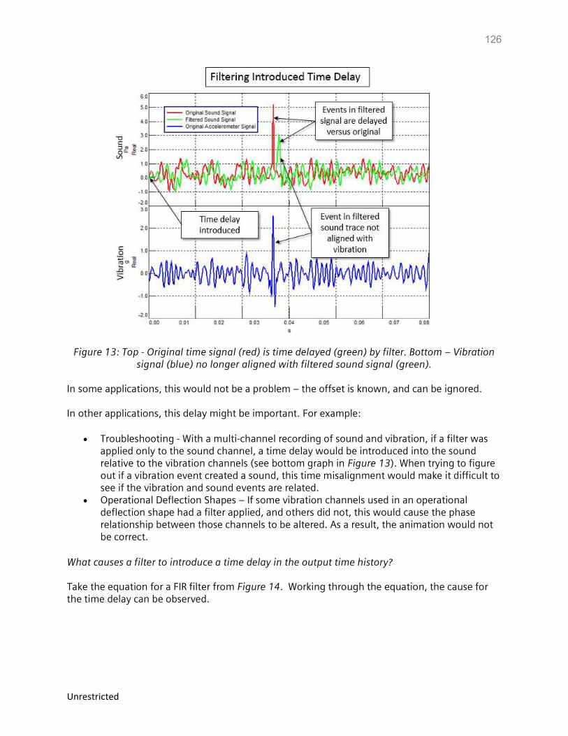
126

Unrestricted

Figure 13: Top - Original time signal (red) is time delayed (green) by filter. Bottom – Vibration signal (blue) no longer aligned with filtered sound signal (green).

In some applications, this would not be a problem – the offset is known, and can be ignored. In other applications, this delay might be important. For example:

Troubleshooting - With a multi-channel recording of sound and vibration, if a filter was applied only to the sound channel, a time delay would be introduced into the sound relative to the vibration channels (see bottom graph in Figure 13). When trying to figure out if a vibration event created a sound, this time misalignment would make it difficult to see if the vibration and sound events are related.

Operational Deflection Shapes – If some vibration channels used in an operational deflection shape had a filter applied, and others did not, this would cause the phase relationship between those channels to be altered. As a result, the animation would not be correct.

What causes a filter to introduce a time delay in the output time history? Take the equation for a FIR filter from Figure 14. Working through the equation, the cause for the time delay can be observed.

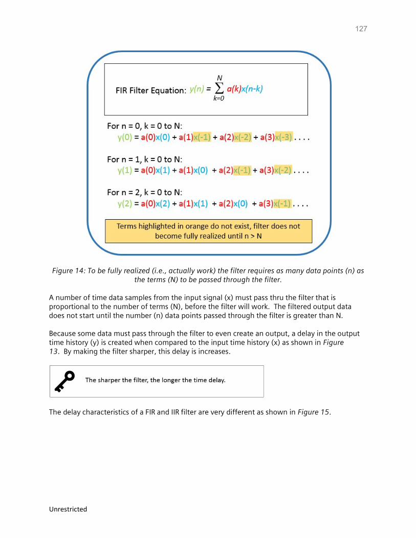
127

Unrestricted

Figure 14: To be fully realized (i.e., actually work) the filter requires as many data points (n) as the terms (N) to be passed through the filter.

A number of time data samples from the input signal (x) must pass thru the filter that is proportional to the number of terms (N), before the filter will work. The filtered output data does not start until the number (n) data points passed through the filter is greater than N. Because some data must pass through the filter to even create an output, a delay in the output time history (y) is created when compared to the input time history (x) as shown in Figure 13. By making the filter sharper, this delay is increases.

The delay characteristics of a FIR and IIR filter are very different as shown in Figure 15.

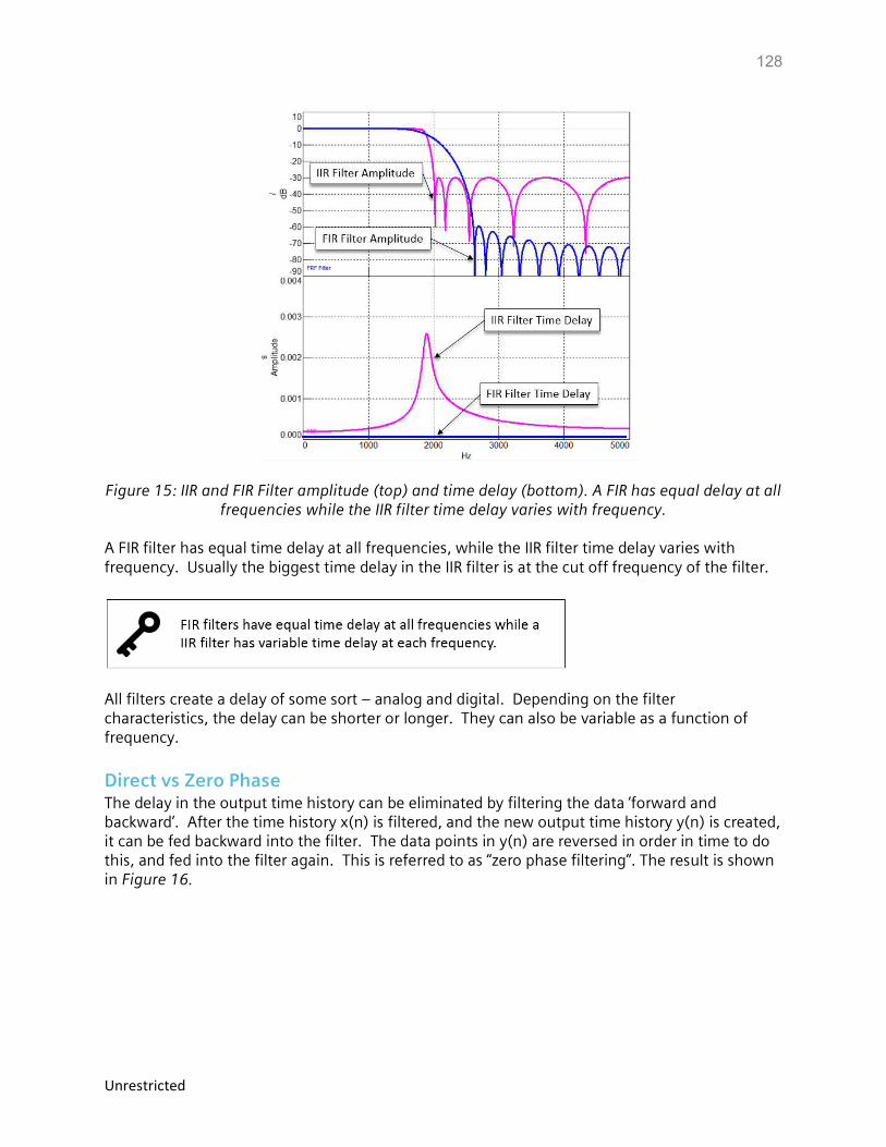
128

Unrestricted

Figure 15: IIR and FIR Filter amplitude (top) and time delay (bottom). A FIR has equal delay at all frequencies while the IIR filter time delay varies with frequency.

A FIR filter has equal time delay at all frequencies, while the IIR filter time delay varies with frequency. Usually the biggest time delay in the IIR filter is at the cut off frequency of the filter.

All filters create a delay of some sort – analog and digital. Depending on the filter characteristics, the delay can be shorter or longer. They can also be variable as a function of frequency.

Direct vs Zero Phase The delay in the output time history can be eliminated by filtering the data ‘forward and backward’. After the time history x(n) is filtered, and the new output time history y(n) is created, it can be fed backward into the filter. The data points in y(n) are reversed in order in time to do this, and fed into the filter again. This is referred to as “zero phase filtering”. The result is shown in Figure 16.

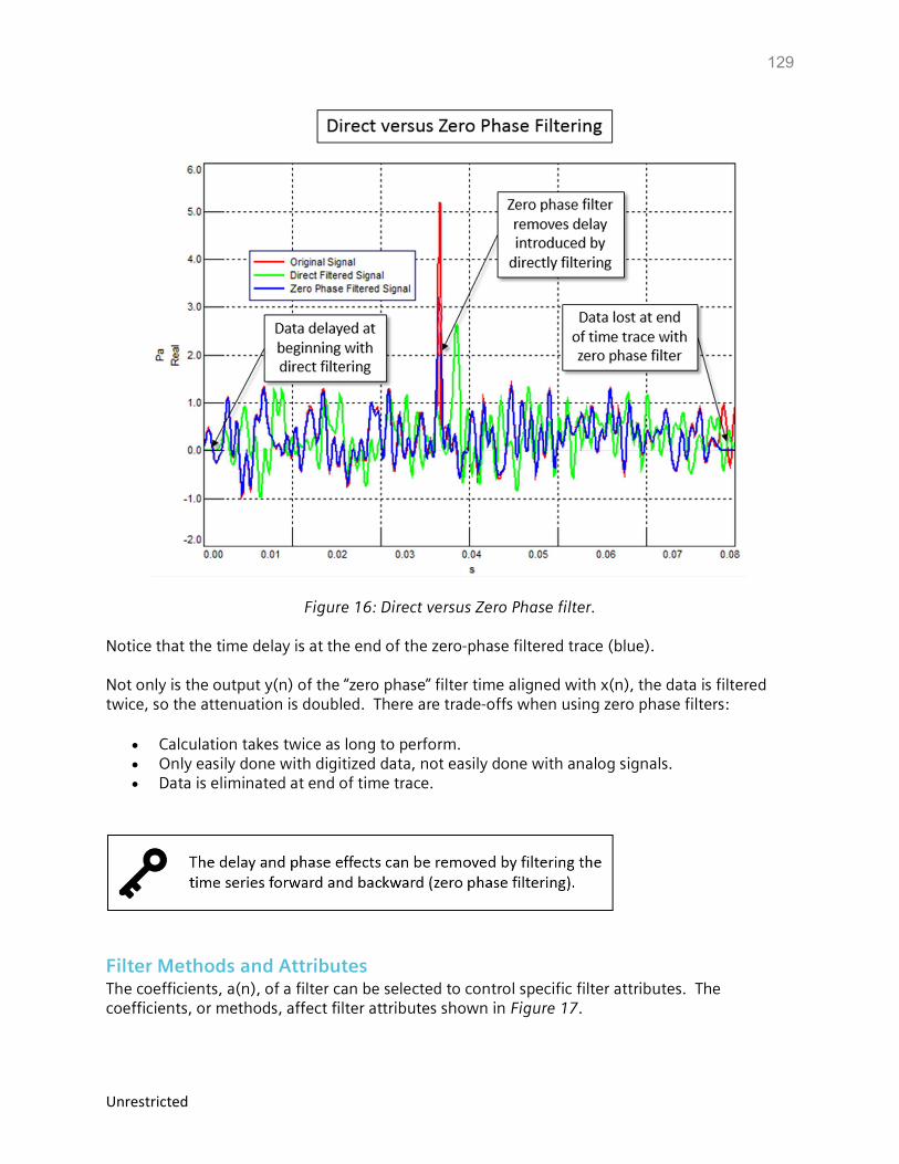
129

Unrestricted

Figure 16: Direct versus Zero Phase filter. Notice that the time delay is at the end of the zero-phase filtered trace (blue). Not only is the output y(n) of the “zero phase” filter time aligned with x(n), the data is filtered twice, so the attenuation is doubled. There are trade-offs when using zero phase filters:

Calculation takes twice as long to perform. Only easily done with digitized data, not easily done with analog signals. Data is eliminated at end of time trace.

Filter Methods and Attributes The coefficients, a(n), of a filter can be selected to control specific filter attributes. The coefficients, or methods, affect filter attributes shown in Figure 17.

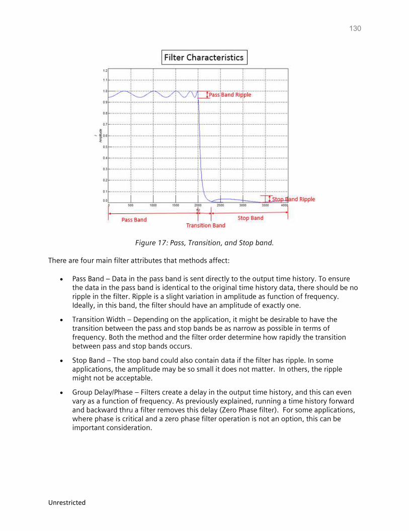
130

Unrestricted

Figure 17: Pass, Transition, and Stop band. There are four main filter attributes that methods affect:

Pass Band – Data in the pass band is sent directly to the output time history. To ensure the data in the pass band is identical to the original time history data, there should be no ripple in the filter. Ripple is a slight variation in amplitude as function of frequency. Ideally, in this band, the filter should have an amplitude of exactly one.

Transition Width – Depending on the application, it might be desirable to have the transition between the pass and stop bands be as narrow as possible in terms of frequency. Both the method and the filter order determine how rapidly the transition between pass and stop bands occurs.

Stop Band – The stop band could also contain data if the filter has ripple. In some applications, the amplitude may be so small it does not matter. In others, the ripple might not be acceptable.

Group Delay/Phase – Filters create a delay in the output time history, and this can even vary as a function of frequency. As previously explained, running a time history forward and backward thru a filter removes this delay (Zero Phase filter). For some applications, where phase is critical and a zero phase filter operation is not an option, this can be important consideration.

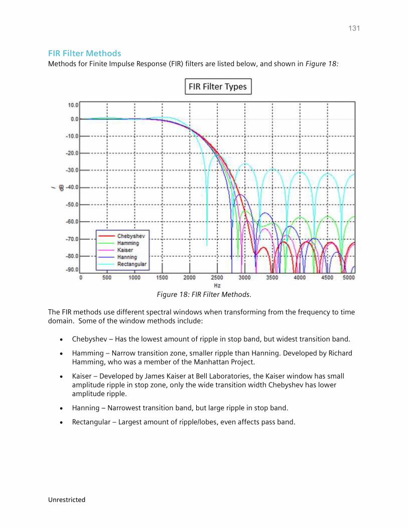
131

Unrestricted

FIR Filter Methods Methods for Finite Impulse Response (FIR) filters are listed below, and shown in Figure 18:

Figure 18: FIR Filter Methods. The FIR methods use different spectral windows when transforming from the frequency to time domain. Some of the window methods include:

Chebyshev – Has the lowest amount of ripple in stop band, but widest transition band.

Hamming – Narrow transition zone, smaller ripple than Hanning. Developed by Richard Hamming, who was a member of the Manhattan Project.

Kaiser – Developed by James Kaiser at Bell Laboratories, the Kaiser window has small amplitude ripple in stop zone, only the wide transition width Chebyshev has lower amplitude ripple.

Hanning – Narrowest transition band, but large ripple in stop band.

Rectangular – Largest amount of ripple/lobes, even affects pass band.

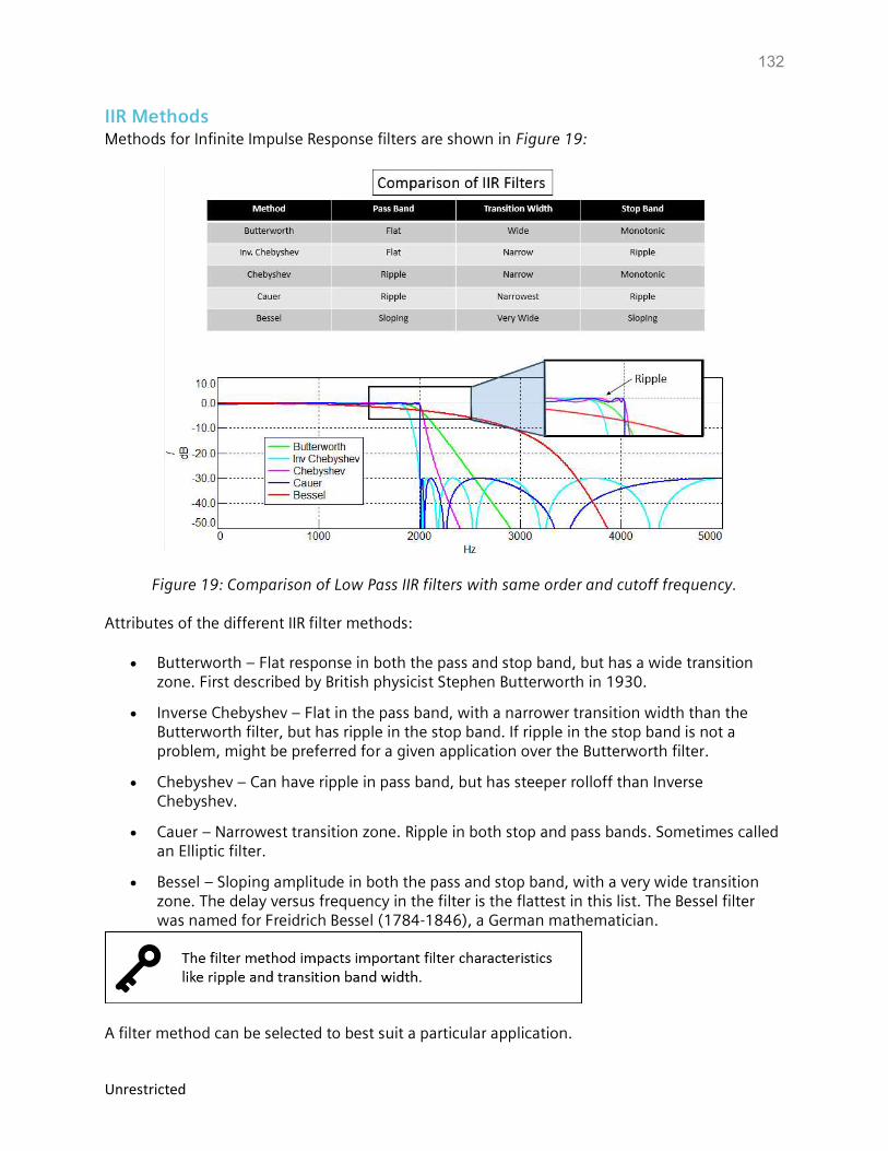
132

Unrestricted

IIR Methods Methods for Infinite Impulse Response filters are shown in Figure 19:

Figure 19: Comparison of Low Pass IIR filters with same order and cutoff frequency. Attributes of the different IIR filter methods:

Butterworth – Flat response in both the pass and stop band, but has a wide transition zone. First described by British physicist Stephen Butterworth in 1930.

Inverse Chebyshev – Flat in the pass band, with a narrower transition width than the Butterworth filter, but has ripple in the stop band. If ripple in the stop band is not a problem, might be preferred for a given application over the Butterworth filter.

Chebyshev – Can have ripple in pass band, but has steeper rolloff than Inverse Chebyshev.

Cauer – Narrowest transition zone. Ripple in both stop and pass bands. Sometimes called an Elliptic filter.

Bessel – Sloping amplitude in both the pass and stop band, with a very wide transition zone. The delay versus frequency in the filter is the flattest in this list. The Bessel filter was named for Freidrich Bessel (1784-1846), a German mathematician.

A filter method can be selected to best suit a particular application.

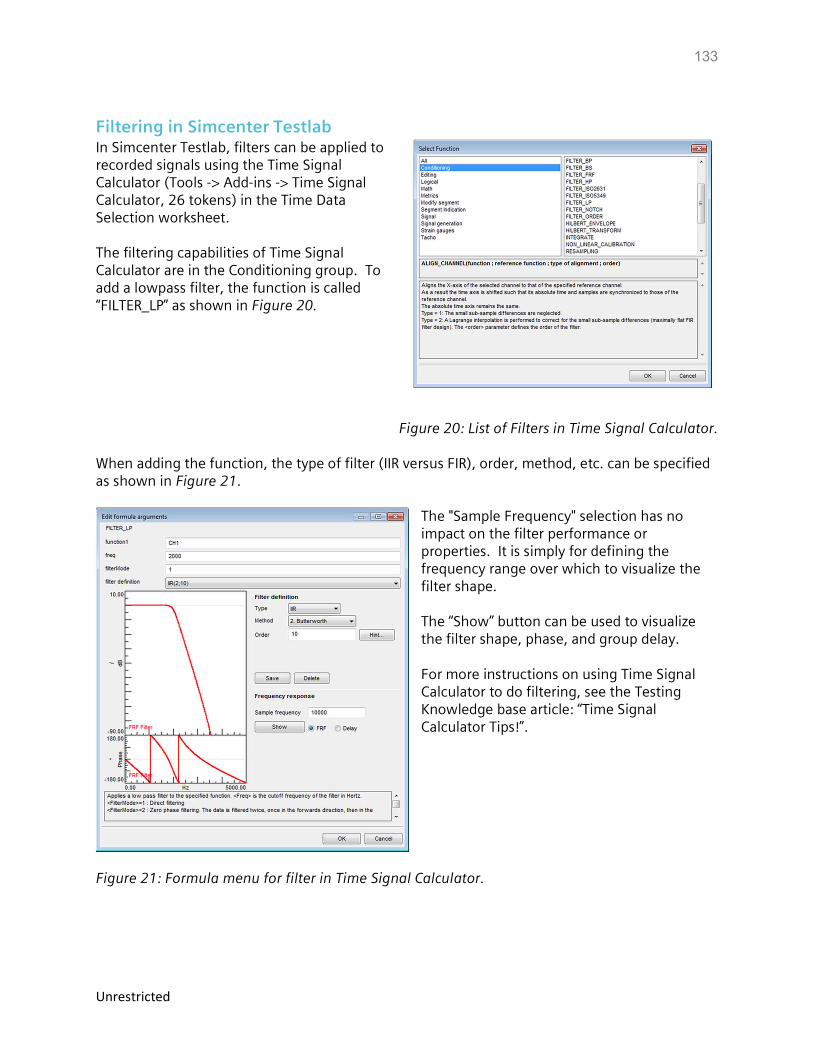
133

Unrestricted

Filtering in Simcenter Testlab In Simcenter Testlab, filters can be applied to recorded signals using the Time Signal Calculator (Tools -> Add-ins -> Time Signal Calculator, 26 tokens) in the Time Data Selection worksheet. The filtering capabilities of Time Signal Calculator are in the Conditioning group. To add a lowpass filter, the function is called “FILTER_LP” as shown in Figure 20.

Figure 20: List of Filters in Time Signal Calculator. When adding the function, the type of filter (IIR versus FIR), order, method, etc. can be specified as shown in Figure 21.

The "Sample Frequency" selection has no impact on the filter performance or properties. It is simply for defining the frequency range over which to visualize the filter shape. The “Show” button can be used to visualize the filter shape, phase, and group delay. For more instructions on using Time Signal Calculator to do filtering, see the Testing Knowledge base article: “Time Signal Calculator Tips!”.

Figure 21: Formula menu for filter in Time Signal Calculator.

Unrestricted

All Articles - Siemens PLM Community Testing Knowledge Base Siemens PLM Community

Digital Signal Processing

What is Fourier Transform? Digital Signal Processing: Sampling Rates, Bandwidth, Spectral Lines, and more... Gain, Range, Quantization Aliasing Overloads Averaging Types: What's the difference? Kurtosis Time-Frequency Analysis: Wavelets Spectrum versus Autopower Autopower Function...Demystified! Power Spectral Density Shock Response Spectrum (SRS) Windows and Leakage Window Types Window correction factors Exponential Window Correction Factors RMS Calculations The Gibbs Phenomenon Introduction to Filters: FIR and IIR

Modal Data Acquisition

Simcenter Testlab Impact Testing Modal Impact Testing: User Defined Impact Sequence What modal impact hammer tip should I use? Modal Tips: Roving hammer versus roving accelerometer Modal Testing: Driving Point Survey – What’s at stake? Attach Modal Shaker at Stiff or Flexible Area of Stucture? Using Pseudo-Random for high quality FRF measurements Multi Input Multi Output MIMO Testing Ground Vibration Testing and Flutter

1

Unrestricted

Modal Analysis and Operational Deflection Shapes

Natural Frequency and Resonance What is Frequency Response Function (FRF)? The FRF and it Many Forms! How to calculate damping from a FRF? Getting Started with Modal Curvefitting Modal Assurance Criterion Simcenter Testlab Modal Analysis: Modification Prediction Import CAD into Simcenter Testlab Animate CAD Geometry Alias Table: Mapping Test Data to Geometry Geometry in Simcenter Testlab Maximum Likelihood estimation of a Modal Model (MLMM) Difference Between Residues and Residuals? What is an Operational Deflection Shape (ODS)? Making a Video of a Time Animation

Acoustics

History of Acoustics Sound Pressure What is a decibel? What is A-weighting? Octaves and Human Hearing What is Sound Power? Decibel Math What is the Acoustic Quantity called Q? Sound Absorption Sound Transmission Loss Noise level certification, how to select the right standard? Sound pressure, sound power, and sound intensity: What is the difference? Sound fields: Free and diffuse field, near and far field

Sound Quality

History of Acoustics Sound Pressure What is a decibel? What is A-weighting? Octaves and Human Hearing Loudness and Sones Calculating a Specific Loudness Spectrum in Simcenter Testlab How to Calculate N10 Time Varying Loudness in Simcenter Testlab?

2

Unrestricted

Articulation Index Auditory Masking Tone-to-Noise Ratio and Prominence Ratio Fluctuation Strength and Roughness Critical Bands in Human Hearing Kurtosis Time-Frequency Analysis: Wavelets Sound Quality Jury Testing Alter Speed of Rotating Sound for Listening Simcenter Testlab Sound Diagnosis

Durability

History of Fatigue Stress and Strain Calculating Damage with Miner's Rule What is a SN-Curve? Rainflow Counting Difference between 'Range-Mean' and 'From-To' Counting Power Spectral Density Shock Response Spectrum (SRS) How to Calculate a Shock Response Spectrum with Testlab? Some Thoughts on Accelerated Durability Testing Goodman-Haigh Diagram for Infinite Life Measuring strain gauges in Simcenter Testlab Rosette Strain Gauges Calculating Damage in Simcenter Tecware Process Builder Strain Gauges: Selecting an Excitation Voltage Simcenter Testlab SCADAS and Long Strain Cables

Rotating Machinery

What is an order? Torsional Vibration: What is it? Zebra Tape Butt Joint Correction for Torsional Vibrations Balancing: Static, Coupled, and Dynamic Removing Spikes from RPM Signals Using the Smoothing function to remove rpm spikes RPM Calculation problems and Laser Tachometers Simcenter Testlab Signature Fixed Sampling versus Synchronous Sampling Tips and tricks for acquiring torsional orders Harmonic Removal Interpreting Colormaps Cycle to Cycle Averaging in Simcenter Testlab

3

Unrestricted

Speed Sweep Data Processing: RPM Increment, Framesize, Sweep Rate, and Overlap Order Cuts: How to Get the Correct Amplitude?

Vibration Control

What is Vibration Control Testing? Vibration Control FAQs Power Spectral Density Shock Response Spectrum (SRS) Sine Control: Estimation Methods Sine Control: Closed Loop Control Parameters Sine Control: Notching Vibration Control: Understanding Selfcheck Direct Field Acoustic Noise Testing What is Total Harmonic Distortion (THD)? Kurtosis "Excessive DC Level" message ITF Warning in Random Vibration Control

Simcenter Testlab General

Simcenter Testlab Overview Simcenter Testlab Active Picture Simcenter Testlab Active Picture Plug-in Download Simcenter Testlab Token Licensing: What is it? How does it work? Simcenter Testlab: Import/Export to Excel Simcenter Testlab: Documentation Tab Simcenter Testlab: Templates Simcenter Testlab: Keyboard and Mouse Shortcuts Simcenter Testlab: CTRL-PageUp and CTRL-PageDown to change worksheets Simcenter Testlab: How to create a custom workflow How to lockdown a test in Simcenter Testlab Simcenter Testlab: Format Based Printing with Powerpoint Simcenter Testlab: Replace Data Origin... Simcenter Testlab: Batch Reporting Nastran and Simcenter Testlab: Viewing Mode Shapes and FRFs Import ANSYS Geometry and Mode Shapes in Simcenter Testlab

Simcenter Testlab Display tips:

Simcenter Testlab: Display Layouts Simcenter Testlab: Customized Legend Text Simcenter Testlab: Curve Linestyles Simcenter Testlab: Cursor Tips and Tricks Simcenter Testlab: Coupled Cursors and Coupled Limits

4

Unrestricted

Simcenter Testlab: Interactive order cursor! Simcenter Testlab: Order Cursor vs Time in Colormap Simcenter Testlab: The "Double X cursor" Simcenter Testlab: Automatic Peak-Valley Cursor Simcenter Testlab: Harmonic Cursors Simcenter Testlab: XY Graph Simcenter Testlab: Keyboard and Mouse Shortcuts Simcenter Testlab: Matrix-Heatmap Display Simcenter Testlab: Replace a curve in a display directly? Simcenter Testlab: Overlay Mode Shapes Simcenter Testlab: Compare data to target quickly with preview mode

Simcenter SCADAS and other Acquisition Hardware

Simcenter SCADAS Mobile and Recorder Hardware Simcenter SCADAS XS: Everything you need to know! Simcenter SCADAS Cable Guide Simcenter Sound Camera Simcenter Soundbrush Qsources: Acoustic and Structural Exciters Simcenter Testlab Smart App Favorites! Single Ended versus Differential Inputs AC versus DC Coupling How to use SCADAS T8 Thermocouple card? ICP versus IEPE versus Charge Accelerometers Long Cable Lengths and ICP Transducers Long cable lengths and strain gauges

Simcenter Testlab Acquisition Tips

Simcenter Testlab Signature Hands-free acquisition (almost) Capturing Transient Events in Simcenter Testlab Cool Channel Setup tricks for Triaxial Accelerometers Copy Channel Setup from One Project to Another? View Channel Setup from Desktop Navigator! Data Acquisition Based on GPS Location How to calculate a VECTOR SUM Tips and tricks for acquiring torsional orders CAN Bus Measurements No more tach! Use OBDII to get engine and vehicle speed... Record Raw CANBUS Data and Decode Offline! Single Plane Balancing in Simcenter Testlab Measuring strain gauges in Simcenter Testlab Correcting a bad calibration factor

5

Unrestricted

Simcenter Testlab Calibration

Simcenter Testlab Time Signal Calculator

Simcenter Testlab: Time Signal Calculator Tips Simcenter Testlab: Calculating Statistics from Time Histories Simcenter Testlab: Appending Time Histories Simcenter Testlab: Create a new recording from a segment cut Simcenter Testlab: Applying an arbitrary filter shape to a time history Simcenter Testlab: Integrating a Time History and Avoiding Offsets Analyzing PWM Signals with Time Signal Calculator Introduction to Filters: FIR vs IIR Applying a Custom Filter Shape: FILTER_FRF command Filter an Order and Listen to It Generate Custom Signals in Time Signal Calculator Removing Spikes from RPM Signals Harmonic Removal Rosette Strain Gauges

Simcenter Testlab Processing Tips

Simcenter Testlab Throughput Processing Tips RPM Extraction in Simcenter Testlab Run Comparison in Simcenter Testlab Order Sections: Setting Parameters Time Signal Calculator Tips Simcenter Testlab: Calculating Statistics from Time Histories Simcenter Testlab: Appending Time Histories Simcenter Testlab: Create a new recording from a segment cut Simcenter Testlab Sound Diagnosis Can I view data in Google Earth? Analyzing PWM Signals in Simcenter Testlab

Simcenter Tecware

Running Simcenter Tecware with Simcenter Testlab tokens Simcenter Tecware: Open Time Files fast! Simcenter Tecware: Overlay multiple signals in X and Y display Simcenter Tecware: Access to different file formats Simcenter Tecware: Spike Filter Simcenter Tecware: Removing Multiple Segments Simcenter Tecware: Calculate Infinite Life with the Goodman Diagram Calculating damage with Simcenter Tecware Processbuilder Butterworth filter "regular" and "zero phase"