Digital Signal Processing Algorithms in Single-Carrier Optical ...

Digital Signal Processing Algorithms in Single-CarrierOptical Coherent Communications

Thèse

Wing-Chau Ng

Doctorat en génie éléctriquePhilosophiæ doctor (Ph.D.)

Québec, Canada

© Wing-Chau Ng, 2015

Résumé

Des systèmes de détection cohérente avec traitement numérique du signal (DSP) sont présente-ment déployés pour la transmission optique de longue portée. La modulation par déplacementde phase en quadrature à deux polarisations (DP-QPSK) est une forme de modulation ap-propriée pour la transmission optique sur de longues distances (1000 km ou plus). Une autreforme de modulation, le DP-16-QAM (modulation d’amplitude en quadrature) a été récem-ment utilisée pour les communications métropolitaines (entre 100 et 1000 km). L’extensionde la distance maximum de transmission du DP-16-QAM est un domaine de recherche actif.Déterminer si l’utilisation de la détection cohérente pour les transmissions à courtes distances(moins de 100 km) en justifieraient les coûts demeure cependant une question ouverte. Danscette thèse, nous nous intéresserons principalement au recouvrement de phase et au démul-tiplexage en polarisation dans les récepteurs numériques cohérents pour les applications àcourte distance.

La réalisation de systèmes optiques gigabauds cohérents en temps-réel utilisant des formats demodulation à monoporteuse plus complexes, comme le 64-QAM, dépend fortement du recou-vrement de phase. Pour le traitement numérique hors-ligne, la récupération de phase utilisantles résultats de décisions (decision-directed phase recovery (DD-PR)) permet d’obtenir, audébit des symboles, les meilleures performances, et ce avec un effort computationnel moindreque celui des meilleurs algorithmes connus. L’implémentation en temps-réel de systèmes gi-gabauds requiert un haut degré de parallélisation qui dégrade de manière significative lesperformances de cet algorithme. La parallélisation matérielle et le délais de pipelinage sur laboucle de rétroaction imposent des contraintes strictes sur la largeur spectrale du laser, ainsique sur le niveau de bruit spectral des sources laser. C’est pourquoi on retrouve peu de dé-monstrations de recouvrement de phase en temps-réel pour les modulations 64-QAM ou pluscomplexes. Nous avons analysé expérimentalement l’impact des lasers avec filtres optiquessur le recouvrement de phase realisé en pipeline sur un système cohérent à monoporteuse 64-QAM à 5 Gbaud. Pour les niveaux de parallélisation plus grands que 24, le laser avec filtresoptiques a permis une amélioration de 2 dB du ratio signal-à-bruit optique, en comparaisonavec le même laser sans filtre optique.

La parallélisation du recouvrement de phase entraîne non seulement une plus grande sensibilité

iii

au bruit de phase du laser, mais aussi une plus grande sensibilité aux fréquences résiduellesinduites par la présence de tonalités sinusoïdales dans la source. La modulation de fréquencessinusoïdales peut être intentionnelle, pour des raisons de contrôle, ou accidentelles, dues àl’électronique ou aux fluctuations environnementales. Nous avons étudié expérimentalementl’impact du bruit sinusoïdal de phase du laser sur le système parallèle de recouvrement dephase dans un système 64-QAM à 5 Gbauds, en tenant compte des effets de la compensationdu décalage de fréquence et de l’égalisation.

De nos jours, les filtres MIMO (multi-input multi-output) à réponse finie (FIR) sont couram-ment utilisés pour le démultiplexage en polarisation dans les systèmes cohérents. Cependant,ces filtres souffrent de divers problèmes durant l’acquisition, tels la singularité (les mêmes don-nées apparaissent dans les deux canaux de polarisation) et la longue durée de convergence decertaines combinaisons d’états de polarisation (SOP). Pour réduire la consommation d’énergieexigée dans les systèmes cohérents pour les applications à courtes distances où le délais degroupe différentiel n’est pas important, nous proposons une architecture DSP originale. Notreapproche introduit une pré-rotation de la polarisation, avant le MIMO, basée sur une estima-tion grossière de l’état de polarisation qui n’utilise qu’un seul paramètre Stokes (s1). Cetteméthode élimine les problèmes de singularité et de convergence du MIMO classique, tout enréduisant le nombre de filtres MIMO croisés, responsables de l’annulation de la diaphonie depolarisation. Nous présentons expérimentalement un compromis entre la réduction de maté-riel et la dégradation des performances en présence de dispersion chromatique résiduelle, afinde permettre la réalisation d’applications à courtes distances.

Finalement, nous améliorons notre méthode d’estimation à l’aveugle par un filtre Kalmanétendu (EKF) à temps discret de faible complexité, afin de réduire la consommation de mé-moire et les calculs redondants apparus dans la méthode précédante. Nous démontrons expé-rimentalement que la pré-rotation de polarisation basée sur le EKF operé au taux ASIC(Application-Specific Integrated Circuits) permet de récupérer la puissance de fréquenced’horloge du signal multiplexé en polarisation ainsi que d’améliorer la performance du tauxd’erreur sur les bits (BER) en utilisant un MIMO de complexité réduite.

iv

Abstract

Coherent detection with digital signal processing (DSP) is currently being deployed in long-haul optical communications. Dual-polarization (DP) quadrature phase shift keying (QPSK)is a modulation format suitable for long-haul transmission (1000 km or above). Anothermodulation, DP-16-QAM (quadrature amplitude modulation) has been deployed recentlyin metro regions (between 100 and 1000 km). Extending the reach of DP-16QAM is anactive research area. For short-reach transmission (shorter than 100 km), there is still anopen question as to when the technology will be mature enough to meet cost pressures forthis distance. In this dissertation, we address mainly on phase recovery and polarizationdemultiplexing in digital coherent receivers for short-reach applications.

Implementation of real-time Gbaud (Gsymbol per second) optical coherent systems for single-carrier higher-level modulation formats such as 64-QAM depends heavily on phase tracking.For offline DSP, decision-directed phase recovery is performed at the symbol rate with thebest performance and the least computational effort compared to best-known algorithms.Real-time implementations at Gbaud requires significant parallelizing that greatly degradesperformance of this algorithm. Hardware parallelization and pipelining delay on the feedbackpath impose stringent requirements on the laser linewidth, or the frequency noise spectrallevel of laser sources. This leads to the paucity of experiments demonstrating real-time phasetracking for 64- or higher QAM. We experimentally investigated the impact of optically-filtered lasers on parallel and pipelined phase tracking in a single-carrier 5 Gbaud 64-QAMback-to-back coherent system. For parallelization levels higher than 24, the optically-filteredlaser shows more than 2 dB improvement in optical signal-to-noise ratio penalty compared tothat of the same laser without optical filtering.

In addition to laser phase noise, parallelized phase recovery also creates greater sensitivity toresidual frequency offset induced by the presence of sinusoidal tones in the source. Sinusoidalfrequency modulation may be intentional for control purposes, or incidental due to electronicsand environmental fluctuations. We experimentally investigated the impact of sinusoidal laserphase noise on parallel decision-directed phase recovery in a 5 Gb 64-QAM system, includingthe effects of frequency offset compensation and equalization.

MIMO (multi-input multi-output) FIR (finite-impulse response) filters are conventionally used

v

for polarization demultiplexing in coherent communication systems. However, MIMO FIRssuffer from acquisition problems such as singularity and long convergence for a certain po-larization rotations. To reduce the chip power consumption required in short-reach coherentsystems where differential group delay is not prominent, we proposed a novel parallelizableDSP architecture. Our approach introduces a polarization pre-rotation before MIMO, ba-sed on a very-coarse blind SOP (state of polarization) estimation using only a single Stokesparameter (s1). This method eliminates the convergence and singularity problems of conven-tional MIMO, and reduces the number of MIMO cross taps responsible for cancelling thepolarization crosstalk. We experimentally presented a tradeoff between hardware reductionand performance degradation in the presence of residual chromatic dispersion for short-reachapplications.

Finally, we extended the previous blind SOP estimation method by using a low-complexitydiscrete-time extended Kalman filter in order to reduce the memory depth and redundantcomputations of the previous design. We experimentally verified that our extended Kalmanfilter-based polarization prerotation at ASIC rates enhances the clock tone of polarization-multiplexed signals as well as the bit-error rate performance of using reduced-complexityMIMO for polarization demultiplexing.

vi

Table des matières

Résumé iii

Abstract v

Table des matières vii

Liste des tableaux xi

Liste des figures xiii

Acknowledgement xix

Avant-propos xxi

Abbreviations xxiii

List of Symbols by Chapter xxv

1 Introduction 11.1 Motivation . . . . . . . . . . . . . . . . . . . . . . . . . . . . . . . . . . . . 11.2 Objectives and Contributions . . . . . . . . . . . . . . . . . . . . . . . . . . 11.3 Organization of thesis . . . . . . . . . . . . . . . . . . . . . . . . . . . . . . 4

2 Phase Recovery Algorithms 72.1 DSP Blocks for Single-Polarization Coherent System . . . . . . . . . . . . . 72.2 Estimation-based Method . . . . . . . . . . . . . . . . . . . . . . . . . . . . 102.3 Detection-based Method . . . . . . . . . . . . . . . . . . . . . . . . . . . . . 142.4 Parallelization and Pipelining . . . . . . . . . . . . . . . . . . . . . . . . . . 162.5 Implementation of DDMLE . . . . . . . . . . . . . . . . . . . . . . . . . . . 182.6 Frequency Noise Power Spectrum Density . . . . . . . . . . . . . . . . . . . 192.7 Summary . . . . . . . . . . . . . . . . . . . . . . . . . . . . . . . . . . . . . 20

3 Optically Filtered Laser 233.1 Introduction . . . . . . . . . . . . . . . . . . . . . . . . . . . . . . . . . . . . 233.2 TeraXion Novel Lasers . . . . . . . . . . . . . . . . . . . . . . . . . . . . . . 243.3 Laser Characterization . . . . . . . . . . . . . . . . . . . . . . . . . . . . . . 263.4 Insight from PSD . . . . . . . . . . . . . . . . . . . . . . . . . . . . . . . . . 273.5 System Performance . . . . . . . . . . . . . . . . . . . . . . . . . . . . . . . 293.6 Conclusions . . . . . . . . . . . . . . . . . . . . . . . . . . . . . . . . . . . . 33

vii

4 Impact of Sinusoidal Phase Modulation on Phase Tracking 354.1 Introduction . . . . . . . . . . . . . . . . . . . . . . . . . . . . . . . . . . . . 364.2 Frequency Offset Compensation Algorithm . . . . . . . . . . . . . . . . . . 384.3 Effect of Residual frequency offset . . . . . . . . . . . . . . . . . . . . . . . 384.4 System Perfomance . . . . . . . . . . . . . . . . . . . . . . . . . . . . . . . . 414.5 Conclusions . . . . . . . . . . . . . . . . . . . . . . . . . . . . . . . . . . . . 45

5 Digital Polarization Demultiplexing 515.1 DSP Blocks in Dual-Polarization Single-Carrier Digital Coherent Receiver . 515.2 Model of fiber polarization effects . . . . . . . . . . . . . . . . . . . . . . . 535.3 Conventional MIMO . . . . . . . . . . . . . . . . . . . . . . . . . . . . . . . 545.4 Role of conventional MIMO . . . . . . . . . . . . . . . . . . . . . . . . . . . 565.5 Problems of conventional MIMO . . . . . . . . . . . . . . . . . . . . . . . . 575.6 Summary . . . . . . . . . . . . . . . . . . . . . . . . . . . . . . . . . . . . . 57

6 SOP Pre-rotation before MIMO 596.1 Introduction . . . . . . . . . . . . . . . . . . . . . . . . . . . . . . . . . . . . 596.2 Proposed DSP Architecture . . . . . . . . . . . . . . . . . . . . . . . . . . . 616.3 SOP-Search Implementation in Stokes Space . . . . . . . . . . . . . . . . . 636.4 Experimental Setup . . . . . . . . . . . . . . . . . . . . . . . . . . . . . . . 656.5 BER performance for various SOPs . . . . . . . . . . . . . . . . . . . . . . . 686.6 Conclusions . . . . . . . . . . . . . . . . . . . . . . . . . . . . . . . . . . . . 726.7 Outpage Probability . . . . . . . . . . . . . . . . . . . . . . . . . . . . . . . 72

7 Extended Kalman Filter-based SOP Pre-rotation 797.1 Contributions . . . . . . . . . . . . . . . . . . . . . . . . . . . . . . . . . . . 797.2 Equations of Extended Kalman Filter . . . . . . . . . . . . . . . . . . . . . 807.3 EKF-based SOP Pre-rotation . . . . . . . . . . . . . . . . . . . . . . . . . . 827.4 Implemenetation . . . . . . . . . . . . . . . . . . . . . . . . . . . . . . . . . 847.5 Performance Analysis . . . . . . . . . . . . . . . . . . . . . . . . . . . . . . 867.6 Conclusion for EKF-based SOP-PR . . . . . . . . . . . . . . . . . . . . . . 88

8 Conclusion 918.1 Future Work . . . . . . . . . . . . . . . . . . . . . . . . . . . . . . . . . . . 92

A Phase Estimation and Phase Tracking 95A.1 Theoretical viewpoint . . . . . . . . . . . . . . . . . . . . . . . . . . . . . . 95A.2 Commercial Systems . . . . . . . . . . . . . . . . . . . . . . . . . . . . . . . 96

B Laser Phase Noise 97

C Reduction in Power Consumption due to Parallelization and Pipelining 101

D Reduction of Tracking Bandwidth 103

E Frequency Noise Power Spectrum Density 105

F Laser Characterization 109F.1 Measurement Techniques for Laser Linewidth . . . . . . . . . . . . . . . . . 109

viii

F.2 Experimental Setup . . . . . . . . . . . . . . . . . . . . . . . . . . . . . . . 110

G Clock Tone and Timing Phase Estimation 113G.1 Introduction . . . . . . . . . . . . . . . . . . . . . . . . . . . . . . . . . . . . 113G.2 Timing Phase Estimation (TPE) . . . . . . . . . . . . . . . . . . . . . . . . 114G.3 Impact of Polarization Effects on TPE . . . . . . . . . . . . . . . . . . . . . 114

H Stokes Space Polarization Demultiplexing 117

I Experimental Generation of Random SOPs 121

J Publication List 123

Bibliographie 125

ix

Liste des tableaux

6.1 Reduction in complex multiplers (CM) and the corresponding reduction per-centage per ASIC clock period for various cross FIR lengths, Ncross, in ourproposed reduced-complexity MIMO, compared to a full-complexity MIMOusing Ncross = 13. . . . . . . . . . . . . . . . . . . . . . . . . . . . . . . . . . . 62

6.2 Cases considered for BER performance analysis. . . . . . . . . . . . . . . . . . 66

xi

Liste des figures

2.1 (a) Element of a single-polarization single-carrier coherent communication sys-tems. (b) Equivalent mathematical model. . . . . . . . . . . . . . . . . . . . . . 8

2.2 Block diagram of decision-directed maximum likelihood phase estimation. . . . 122.3 Symbols classification used in Viterbi-Viterbi algorithm (modified for MQAM)

in (a) Seimetz’s work [52] and (b) Gao et al.’s work [13] . . . . . . . . . . . . . 132.4 Block diagrams of feedforward blind phase search, reproduced from Fig. 4 in

[44]. . . . . . . . . . . . . . . . . . . . . . . . . . . . . . . . . . . . . . . . . . . 152.5 B test phases in a quadrant. Background : 16-QAM with uncompensated phase

noise [44]. . . . . . . . . . . . . . . . . . . . . . . . . . . . . . . . . . . . . . . . 162.6 Implementation of decision-direct maximum likelihood estimation for a time-

interleaved structure [75]. . . . . . . . . . . . . . . . . . . . . . . . . . . . . . . 172.7 Equivalence of implementation of DD-MLE with feedback delay. . . . . . . . . 192.8 Laser Frequency noise power spectral density. . . . . . . . . . . . . . . . . . . . 20

3.1 Transmission spectrum of the FBG assembly. [2] . . . . . . . . . . . . . . . . . 253.2 Frequency locking schematic. TEC : thermoelectric cooler. [2] . . . . . . . . . . 253.3 Cartoon of frequency-noise power spectral density for a laser with active fre-

quency noise reduction. . . . . . . . . . . . . . . . . . . . . . . . . . . . . . . . 263.4 FN-PSD of native mode (without FBG) and low-noise mode (with FBG). . . . 283.5 Top : experimental setup of back-to-back 5-Gbaud 64-QAM. Right bottom :

Recovered 64 QAM constellation without parallelization at OSNR = 28 dB(BER= 6e-5). IQ mod : In-phase/Quadrature modulator, AWG : Arbitrarywaveform generator, PM fiber : Polarization maintaining fiber, VOA : variableoptical attenuator, OBPF : optical bandpass filter, PC : polarization controller.Coh. Rx. : Coherent Receiver. RTO : Real time oscilloscope. EDFA : Erbiumdoped fiber amplifier. . . . . . . . . . . . . . . . . . . . . . . . . . . . . . . . . 30

3.6 BER versus OSNR for native and low-noise mode of PS-TNLs for serial andparallel phase tracking (d = 4) with P = 12 and P = 24. . . . . . . . . . . . . 31

3.7 OSNR penalty for back-to-back 5 Gbaud 64-QAM with d = 4 versus paralleli-zation (lower axis) and versus bandwidth of phase tracking loop (upper axis)for both native mode and low-noise mode. Shaded area is the noise suppressionband, i.e., in Fig. 3.4 where low-noise FN-PSD falls below native FN-PSD. . . . 33

3.8 Constellations over 30 000 symbols, P = 26, d = 4, OSNR = 32 dB for (a)native mode (BER = 1e-3) and (b) low-noise mode (BER = 4e-4). . . . . . . . 33

4.1 Block diagram of a single-polarization, single-carrier coherent system. . . . . . 37

xiii

4.2 Simulated laser phase. Blue : sine tone with Wiener phase noise ; Red : pureWiener phase noise . . . . . . . . . . . . . . . . . . . . . . . . . . . . . . . . . . 39

4.3 Simulated impact of FOC within a time window of LDS = 8000 symbols chosenin the linear region of the laser phase. Left : before FOC ; Right : After FOC. . 40

4.4 Simulated impact of FOC within a time window of LDS = 8000 symbols chosenin proximity of the sine tone maxima. Left : before FOC ; Right : After FOC. . 40

4.5 Simulated impact of FOC within a time window of LDS = 12000 symbols chosenin proximity of the sine tone maxima. Left : before FOC ; Right : After FOC. . 41

4.6 Frequency noise PSD of our laser under test (blue : white noise filtered ITLA).Source : TeraXion PS-TNL specification. . . . . . . . . . . . . . . . . . . . . . . 41

4.7 Experimental setup of back-to-back 5-Gbaud 64-QAM. IQ Mod. : in phase-quadrature modulator, AWG : Arbitrary waveform generator, PM : polarizationmaintaining, VOA : variable optical attenuator, OBPF : optical bandpass filter.PC : polarization controller. Coh. Rx. : Coherent Receiver. RTO : Real timeoscilloscope. EDFA : Erbium doped fiber amplifier. Right : Recovered 64 QAMconstellation without parallelization at OSNR = 28 dB (BER = 6e-5). . . . . . 42

4.8 Experimental OSNR penalty vs. levels of parallelization for (a) no FM, (b)sinusoidal FM, fm = 25 kHz, App = 0.6 MHz, (c) sinusoidal FM, fm = 75 kHz,App = 1.5 MHz. Right : the best constellations at received OSNR = 28 dB foreach case. . . . . . . . . . . . . . . . . . . . . . . . . . . . . . . . . . . . . . . . 47

4.9 (a) True laser phase with an FM of 75 kHz over 60 000 symbols (b) true laserphase noise from 12001th symbols to 24000th symbols (c) true phase, phaseestimated by serial DD-MLE, phase estimated by parallel DD-MLE with P = 8. 48

4.10 OSNR penalty for sweeping fm from 25 kHz to 75 kHz, App from 0.5 MHz to1.5 MHz. for (a) P = 8 (b) P = 10 (c) P = 12. All corresponds to LDS = 8k. . 49

5.1 The main blocks of digital signal processing in a single-carrier coherent receivers 52

6.1 DSP architecture with reduced cross-FIR taps. CDC : chromatic dispersioncompensation. ADC : analog-to-digital conversion. SS-SOP : Stokes space stateof polarization. . . . . . . . . . . . . . . . . . . . . . . . . . . . . . . . . . . . . 61

6.2 Principle of SOP estimation based on s1-MMSD. (a) Before polarization rota-tion ; (b) after polarization rotation according to S1-MMSD. . . . . . . . . . . . 63

6.3 Implementation of feedforward blind SOP search based on s1 parameter atevery 4th ASIC clock. . . . . . . . . . . . . . . . . . . . . . . . . . . . . . . . . 63

6.4 The surface of the mean squared distance (MSD) of S1 parameter. Red dotrefers to the MMSD (the optimal SOP). . . . . . . . . . . . . . . . . . . . . . 65

6.5 Experimental setup for 32 Gbaud DP-QPSK 40 km transmission. PC : Polari-zation controller, IQ Mod. : Inphase-Quadrature modulator, Pol. Syn. : Polari-zation synthesis, OBPF : optical band pass filter, OTDL : Optical tunable delayline, OSA : optical spectrum analyser, RTO : real-time oscilloscope, EDFA :erbium doped fiber amplifier, VOA : variable optical attenuator, Coh. Rx. :Coherent receiver. . . . . . . . . . . . . . . . . . . . . . . . . . . . . . . . . . . 66

xiv

6.6 Comparison in BER performance between the conventional MIMO-FIR (red),our approach with SOP estimation/PR (blue) and the reduced-complexityMIMO without SOP estimation/PR (black) in the presence of 40 km-SMFtransmission (a) Black : 7 cross taps without SOP prerotation ; with tap initialization∗.Blue : 7 cross taps with SOP prerotation. Red : 13 cross taps with SOP prerota-tion. (b) Black : 5 cross taps without SOP prerotation ; with tap initialization∗.Blue : 5 cross taps with SOP prerotation. Red : 13 cross taps with SOP prerota-tion. All above were generated using 10 degree-resolution blind SOP search.(*)Without SOP prerotation, MIMO convergence must be assisted with prior in-formation of SOP. This prior SOP can be obtained from the best case (case A ;full-complexity MIMO) after all taps converge, and is then used to initializethe FIR taps for case C (reduced-complexity MIMO without SOP-PR). . . . . 68

6.7 The mean and the standard deviation of taps of MIMO-FIRs correspondingto the results in Fig. 6.6 when using (a) Black : 7 cross taps without SOPprerotation ; with tap initialization. Blue : 7 cross taps with SOP prerotation.Red : 13 cross taps with SOP prerotation. (b) Black : 5 cross taps withoutSOP prerotation ; with tap initialization only. Blue : 5 cross taps with SOPprerotation. Red : 13 cross taps with SOP prerotation. All above were generatedusing 10 degree-resolution blind SOP search. All above were generated using 10degree-resolution blind SOP search, averaged over 245 unrepeated SOPs with10 realizations for each SOP. PR : Prerotation. . . . . . . . . . . . . . . . . . . 74

6.8 Comparison in BER performance between (a) using 10-degree resolution blindSOP search and (b) 1-degree resolution blind SOP search for our reducedMIMO with 5 cross taps only. The above results were obtained after a 40-kmFD-CDC. . . . . . . . . . . . . . . . . . . . . . . . . . . . . . . . . . . . . . . . 75

6.9 The probability mass functions of BER conditioned on different OSNR valuesof our proposed DSP after 40 km SMF transmission, with 10-degree resolutionin our coarse SOP estimation. Green : 5 cross taps with zero CDC (residual CD= 680ps/nm) ; Red : 5 cross taps with 20-km CDC (residual CD = 340ps/nm) ;blue : 5 cross taps with 40-km CDC ; BER curves correspond-ing to 245 differentSOPs were shown for each case. . . . . . . . . . . . . . . . . . . . . . . . . . . . 76

6.10 Comparison of clock tone magnitudes between the DSP without (red) andwith SOP-PR (black ; our proposed DSP) over 780 various unrepeated SOPsgenerated by a polarization synthesizer at OSNR of 10 dB. A.u. : arbitrary unit. 77

7.1 (a) Our proposed DSP flow. ADC : analog-to-digital converter, CDC : chro-matic dispersion compensation, SOP : state-of-polarization. EKF : extendedKalman filter (b) SOP prerotation (c) our extended Kalman filter flow chat.Blue rectangles : pipelining delays. . . . . . . . . . . . . . . . . . . . . . . . . . 84

7.2 Implementation diagram of our EKF-based SOP-PR . . . . . . . . . . . . . . . 857.3 (a) Evolution of state variables (parameters of Jones matrix). (b) Comparison

of clock tone magnitudes within 18000 ASIC clock cycles before and after EKF-based SOP-PR. (c) Comparison of clock tone magnitudes over a longer duration(over 332000 ASIC clock cycles) before and after EKF-based SOP-PR. All plotswere generated using polarization-scrambled (at 50 kHz) 32 Gbaud DP-QPSKat OSNR = 16 dB. . . . . . . . . . . . . . . . . . . . . . . . . . . . . . . . . . . 87

xv

7.4 Comparison of bit error rates (measured every minute) of using reduced-complexityMIMO filter taps (Ncross = 7) proposed in Chapter 6 with and without EKF-based SOP-PR. All plots were generated using polarization-scrambled (at 50kHz) 32 Gbaud DP-QPSK at OSNR = 16 dB. . . . . . . . . . . . . . . . . . . 89

7.5 Comparison of bit error rates versus OSNRs of using reduced-complexity MIMOfilter taps (Ncross = 7) in Chapter 6 with and without EKF-based SOP-PR,and using a full-complexity MIMO with EKF-based SOP-PR. All points weregenerated using polarization-scrambled (at 50 kHz) 32 Gbaud DP-QPSK . . . 89

F.1 Experimental setup of the delayed self-homodyne coherent detection. . . . . . . 110

G.1 (a) Clock tone magnitude and (b) clock tone phase of received signal either onX-polarization under the effect of polarization angle and DGD. The receiverbandwidth is 0.7 Baud. A.u. : arbitrary unit. . . . . . . . . . . . . . . . . . . . 115

I.1 (a) A sphere and a right cylinder circumscribed about the sphere. Sphericalpoints P and area S and the corresponding axial projections P’ and S’ on thecylindrical surface. (b) Differential area dS on the sphere and its axial projectiondS’ on the cylinder. . . . . . . . . . . . . . . . . . . . . . . . . . . . . . . . . . 121

I.2 The results of random spherical sampling showing (a) 1000 random SOPs ; (b)500 random SOPs (interleaved from (a) ) ; (c) 250 random SOPs (interleavedfrom (a) ). . . . . . . . . . . . . . . . . . . . . . . . . . . . . . . . . . . . . . . . 122

xvi

To my mother, Kam-Ying Lee.

xvii

Acknowledgement

First and foremost, I would like to express my gratitude to my advisor, Prof. Leslie A. Ruschfor her support, resources, advice, experience and guidance in the completion of this work.

I would also show my thank to Dr. An T. Nguyen, of Université Laval, who is responsiblefor experiments, equipment, signal generation, transmitter signal equalization, fiber optics,advices and feedback on my digital signal processings.

Many thanks and much appreciation are owed to Dr. Chul-Soo Park, of Université Laval, whois a very professional laboratory manager and research scientist in our optical communicationlaboratory, responsible for experiment, equipment, signal generation, transmitter and receiverhardware, advices and guidance on the equipment handling and maintenance.

I also thank our laboratory technician Mr. Philippe Chrétien for his great help in providingspeedy support in laboratory tools, logistics, safety guidance, equipment handling.

I would like to thank Dr. Qunbi Zhuge of McGill University for technical discussion in ourcountless email correspondances. His explaination on his paper about parallelization andsuperscalar structure for phase tracking contributed a lot in my first project in Chapter 3.

I also express my gratitude to the following persons, without priority, for their fruitful tech-nical discussion on timing phase recovery in coherent communications : Yuliang Gao of HongKong Polytechnic University, Meng Qiu, Xian Xu and Wei Wang of McGill University, whichcontributes a lot of my understanding and leads to my work in Chapter 6 and in AppendixG.

I would also thank Dr. Peter Winzer of Bell Labs, New Jersey, for being responsible and activefor replying emails even though I am only an unimportant figure in the research field ; Dr.Xi Chen of University of Melbourne for her email correspondence regarding the experimentalsetup of laser linewidth characterization ; Dr. Kai Shi of Dublin City University for his emailcorrespondence regarding the experimental setup of laser linewidth characterization ; Dr. Ro-bert Maher of University College of London for his email correspondence regarding his paperon dynamic linewidth measurement ; Dr. F. Vacondio of Bell Labs, Paris, for notifying me thepaper from Kikuchi [26] in an email correspondence in 2012.

xix

Special thanks are also given to the colleague, Mr. Charles Brunet, for his time to translate mythesis abstract from English to French, and to the following past colleagues : Dr. AmirhosseinGhazisaeidi, for his political correctness and generous enlightenment in my system work ; Dr.Qing Xu, for his countless extra hours helping me finish my experiment during my visit inMay 2010 ; Dr. Mehrdad Mirshafiei, for his unlimited information about the living in QuébecCity and for his friendly support.

Upon the completion of the final version of this dissertation, I would thank Mr. JiachuanLin and Mr. Zhihui Cao, of Université Laval for their prompt responses and their help incoordinating computers for me to compute the results required.

Last but not least, I express my gratitude to my mother and my sister for their patience,spiritual and financial support to let me study further after the completion of my master ofapplied science degree at University of Toronto ; to Prof. Chester Shu, Prof. Hong-Ki Tsangand Prof. Kong-Pan Poon, of the Chinese University of Hong Kong, for their support andopinions on my graduate studies, and to my secondary-school teacher, Mr. Wai-Shing Chan,for his enlightenment and rational advice for every decision I made for my life.

xx

Avant-propos

Publications related to this thesis

1. W. C. Ng, A. T. Nguyen, S. Ayotte, C. S. Park, and L. A. Rusch, “Overcoming PhaseSensitivity in Real-time Parallel DSP for Optical Coherent Communications : OpticallyFiltered Lasers,” IEEE J. Lightw. Technol., Vol. 32, No. 3, pp. 411 - 420 Feb. 2014.http://ieeexplore.ieee.org/xpl/articleDetails.jsp?tp=&arnumber=6678710

The problem (focusing on parallelized phase tracking) was defined by L. A. Rusch. Dr.Simon Ayotte of TeraXion collaborated with us and provided access to narrow linewidthTeraXion sources for use in our experimental demonstrations. The aim of this paper isto experimentally investigate the regimes where the TeraXion narrow-linewidth lasersoutperform conventional lasers.I was responsible for digital signal processing (DSP) and data analysis. A. T. Nguyen andC.-S. Park were responsible for the experimental setup. The first experiment of back-to-back 16-QAM was first set up by Chul-Soo Park in August/September 2012 for bit-errorrate measurement for M-QAM for a conference paper [39]. In March 2013, An T. Nguyenperformed an experiment of predistortion of 64-QAM transmitted data. I performed themeasurement of the bit error rate (BER) versus optical signal-to-noise ratio (OSNR).Finally, I wrote the entire paper, with many helpful comments/suggestions from allcoauthors. Please refer to Chapter 3.

2. W. C. Ng, A. T. Nguyen, S. Ayotte, C. S. Park, and L. A. Rusch, “Impact of SinusoidalTones on Parallel Decision-Directed Phase Recovery for 64-QAM,” IEEE PhotonicsLetters Technology, Vol. 26, No. 5, pp. 486 - 489, Mar. 2014. http://ieeexplore.

ieee.org/xpl/articleDetails.jsp?tp=&arnumber=6701345

I proposed this research topic, finding out the parameters of sine tones (for controlpurposes) of laser sources that do not result in failure of parallel phase tracking algorithmwith feedback delay.I was responsible for all DSP and data analysis. An T. Nguyen and Chul-Soo Park wereresponsible for experimental setup. An T. Nguyen performed the 64-QAM predistortion.I performed the measurement of the bit error rates. All coauthors provided valuablecomments/suggestions on the text. Please refer to Chapter 4.

xxi

3. W. C. Ng, A. T. Nguyen, C. S. Park, and L. A. Rusch, “Reduction of MIMO-FIRTaps via SOP-Estimation in Stokes Space for 100 Gbps Short Reach Applications,”European Conference and Exhibition on Optical Communication, P3.3, September, 2014.http://ieeexplore.ieee.org/xpl/articleDetails.jsp?arnumber=6963901

I proposed this research topic, a novel DSP architecture to accelerate algorithm conver-gence and restore the clock tone to avoid system failure in a single-carrier coherent re-ceiver. The architecture reduces the power consumption (hardware) of the single-carriercoherent receiver chips for short-reach application.I was responsible for algorithm design, digital signal processing (DSP) and data ana-lysis. An T. Nguyen and Chul-Soo Park were responsible for experimental setup. Theexperiment of 40-km single-mode fiber (SMF) 32 Gbaud DP-QPSK was set up by AnT. Nguyen, with the assistance of Chul-Soo Park.Finally, I wrote the entire paper, withmany helpful comments and suggestions from all coauthors. Please refer to Chapter 6.

4. W. C. Ng, A. T. Nguyen, C. S. Park, and L. A. Rusch, “Enhancing Clock Tonevia Polarization Pre-rotation : A Low-complexity, Extended Kalman Filter-based Ap-proach,”Optical Fiber Communication Conference, paper Th2A.19, March 2015.I proposed this research topic, a low-complexity algorithm using the extended Kalmanfilter to further reduce the hardware consumption required in the previous work.I was responsible for algorithm design, DSP and data analysis. An T. Nguyen and Chul-Soo Park were responsible for the experimental setup. The experiment of 40-km single-mode fiber (SMF) 32Gbaud DP-QPSK was set up by An T. Nguyen in March/April2014, with the assistance of Chul-Soo Park. Finally, I wrote the entire paper, with manyhelpful comments and suggestions from all coauthors. Please refer to Chapter 7.

xxii

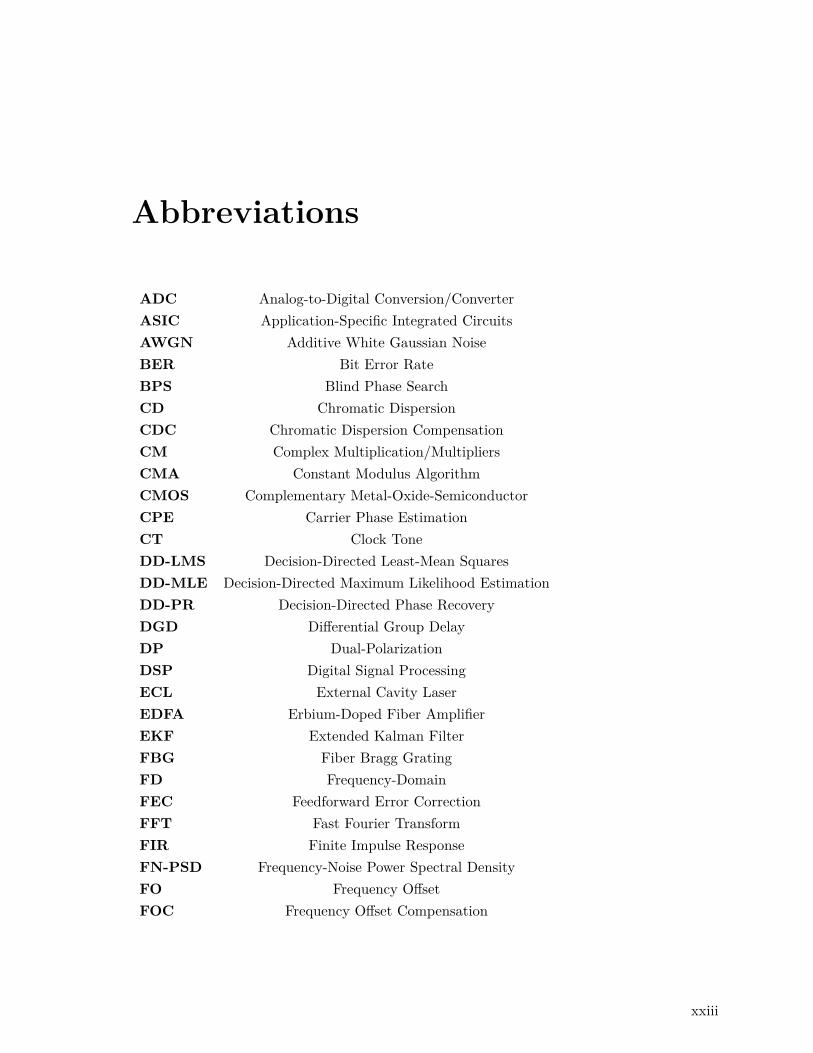
Abbreviations

ADC Analog-to-Digital Conversion/ConverterASIC Application-Specific Integrated CircuitsAWGN Additive White Gaussian NoiseBER Bit Error RateBPS Blind Phase SearchCD Chromatic DispersionCDC Chromatic Dispersion CompensationCM Complex Multiplication/MultipliersCMA Constant Modulus AlgorithmCMOS Complementary Metal-Oxide-SemiconductorCPE Carrier Phase EstimationCT Clock ToneDD-LMS Decision-Directed Least-Mean SquaresDD-MLE Decision-Directed Maximum Likelihood EstimationDD-PR Decision-Directed Phase RecoveryDGD Differential Group DelayDP Dual-PolarizationDSP Digital Signal ProcessingECL External Cavity LaserEDFA Erbium-Doped Fiber AmplifierEKF Extended Kalman FilterFBG Fiber Bragg GratingFD Frequency-DomainFEC Feedforward Error CorrectionFFT Fast Fourier TransformFIR Finite Impulse ResponseFN-PSD Frequency-Noise Power Spectral DensityFO Frequency OffsetFOC Frequency Offset Compensation

xxiii

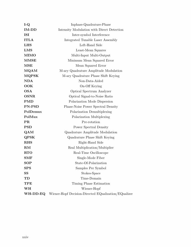
I-Q Inphase-Quadrature-PhaseIM-DD Intensity Modulation with Direct DetectionISI Inter-symbol InterferenceITLA Integrated Tunable Laser AssemblyLHS Left-Hand SideLMS Least-Mean SquaresMIMO Multi-Input Multi-OutputMMSE Minimum Mean Squared ErrorMSE Mean Squared ErrorMQAM M-ary Quadrature Amplitude ModulationMQPSK M-ary Quadrature Phase Shift KeyingNDA Non-Data-AidedOOK On-Off KeyingOSA Optical Spectrum AnalyzerOSNR Optical Signal-to-Noise RatioPMD Polarization Mode DispersionPN-PSD Phase-Noise Power Spectral DensityPolDemux Polarization DemultiplexingPolMux Polarization MultiplexingPR Pre-rotationPSD Power Spectral DensityQAM Quadrature Amplitude ModulationQPSK Quadrature Phase Shift KeyingRHS Right-Hand SideRM Real Multiplication/MultiplierRTO Real-Time OscilloscopeSMF Single-Mode FiberSOP State-Of-PolarizationSPS Samples Per SymbolSS Stokes-SpaceTD Time-DomainTPE Timing Phase EstimationWH Wiener-HopfWH-DD-EQ Wiener-Hopf Decision-Directed EQualization/EQualizer

xxiv

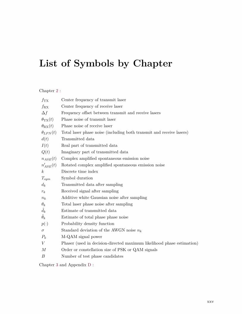
List of Symbols by Chapter

Chapter 2 :

fTX Center frequency of transmit laserfRX Center frequency of receive laser∆f Frequency offset between transmit and receive lasersθTX(t) Phase noise of transmit laserθRX(t) Phase noise of receive laserθLPN (t) Total laser phase noise (including both transmit and receive lasers)d(t) Transmitted dataI(t) Real part of transmitted dataQ(t) Imaginary part of transmitted datanASE(t) Complex amplified spontaneous emission noisen′ASE(t) Rotated complex amplified spontaneous emission noisek Discrete time indexTsym Symbol durationdk Transmitted data after samplingrk Received signal after samplingnk Additive white Gaussian noise after samplingθk Total laser phase noise after samplingdk Estimate of transmitted dataθk Estimate of total phase phase noisep(·) Probability density functionσ Standard deviation of the AWGN noise nkPk M-QAM signal powerV Phaser (used in decision-directed maximum likelihood phase estimation)M Order or constellation size of PSK or QAM signalsB Number of test phase candidates

Chapter 3 and Appendix D :

xxv

ϕb Test phase angle for blind phase searchXk,b Output of the decision device for blind phase searchYk The sampled received signal for blind phase searchP Number of parallelizationd Number of pipelining delay elementsU Phase incrementS∆f Frequency noise power spectral density levelS∆f,BM Frequency noise power spectral density level due to Brownian-motion laser phase noiseS∆f,AWGN Frequency noise power spectral density level due to the AWGN noise from electronics or EDFAA Amplitude of electric field of the receiver signal in the absence of noiseNo Two-sided field power spectral density of the AWGN noiseTloop Response time of the feedback loop of parallel DD-MLERs Symbol rateK Proportionality constant

Chapter 4 :

∆fFO Frequency offset estimateLFFT Block size of fast Fourier transformfc Laser carrier frequencyApp Peak-to-peak frequency-modulated amplitudefm Frequency-modulated frequencyLDS Length of data segment used to undergo FOC

Chapter 5 :

θ Polarization orientation angleφ Phase delay between the optical fields on X and Y polarizationsτ Differential group delay (DGD) due to polarization mode dispersion (PMD)Xkin Input sequence of MIMO for X-polarization

Y kin Input sequence of MIMO for Y-polarizationXout Output of MIMO (after equalization and polarization de-rotation) for X-polarizationYout Output of MIMO (after equalization and polarization de-rotation) for Y-polarizationhki,j FIR filters in MIMO, where i and j can be x or yµ Step-size parameter for updating adaptive FIR filters∇J Averaged error signal depending on the criterion used for equalization∇JCMA Averaged error signal based on CMAA Electric field or vector on either X or Y-polarizationex Instantaneous error signal based on CMA, calculated based on the X output of MIMOey Instantaneous error signal based on CMA, calculated based on the Y output of MIMO

Chapter 6 :

xxvi

s Estimated state-of-polarizationsi Stokes parameters, where i can be 1, 2 or 3θ Estimated polarization orientation angleφ Estimated phase delay between the optical fields on X and Y polarizationsEx Complex field in X-polarizationEy Complex field in Y-polarization

Chapter 7 :

xk State vectorxk Posteriori estimate of xkx−k Priori estimate of xkζk−1 Process noiseuk External perturbationξk Measurement noisezk Measurement outputh Measurement systemQ Process-noise covariance varianceR Measurement-noise covariance varianceH Jacobian matrix of partial derivatives of function hKk Kalman gainPk−1 Covariance matrix of estimation errorP−k Covariance matrix of estimation error after the adjustment

using the knowledge of parameter dynamics A and process noise Qx0 Initial statem0 Mean of initial state x0

P0 Covariance matrix of initial state x0

JPR Jones matrix for pre-rotationXin X-polarization input of JPRYin Y-polarization input of JPRXout X-polarization output of JPRYout Y-polarization output of JPR

Appendix B and Appendix F :

xxvii

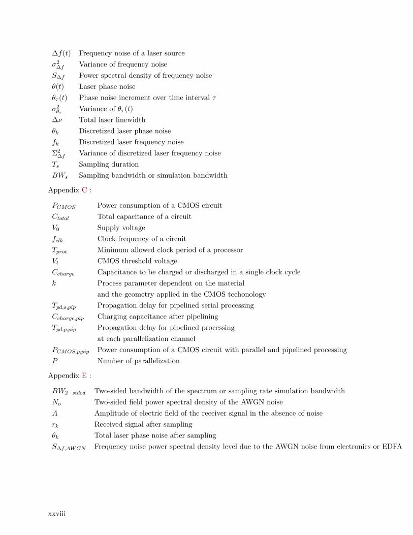
∆f(t) Frequency noise of a laser sourceσ2

∆f Variance of frequency noiseS∆f Power spectral density of frequency noiseθ(t) Laser phase noiseθτ (t) Phase noise increment over time interval τσ2θτ

Variance of θτ (t)∆ν Total laser linewidthθk Discretized laser phase noisefk Discretized laser frequency noiseΣ2

∆f Variance of discretized laser frequency noiseTs Sampling durationBWs Sampling bandwidth or simulation bandwidth

Appendix C :

PCMOS Power consumption of a CMOS circuitCtotal Total capacitance of a circuitV0 Supply voltagefclk Clock frequency of a circuitTproc Minimum allowed clock period of a processorVt CMOS threshold voltageCcharge Capacitance to be charged or discharged in a single clock cyclek Process parameter dependent on the material

and the geometry applied in the CMOS techonologyTpd,s,pip Propagation delay for pipelined serial processingCcharge,pip Charging capacitance after pipeliningTpd,p,pip Propagation delay for pipelined processing

at each parallelization channelPCMOS,p,pip Power consumption of a CMOS circuit with parallel and pipelined processingP Number of parallelization

Appendix E :

BW2−sided Two-sided bandwidth of the spectrum or sampling rate simulation bandwidthNo Two-sided field power spectral density of the AWGN noiseA Amplitude of electric field of the receiver signal in the absence of noiserk Received signal after samplingθk Total laser phase noise after samplingS∆f,AWGN Frequency noise power spectral density level due to the AWGN noise from electronics or EDFA

xxviii

Chapitre 1

Introduction

1.1 Motivation

Complex modulation with coherent detection system offers much greater spectral efficiencythan intensity modulation with direct detection (IM-DD). Using coherent detection, both am-plitude and phase can be retrieved at the receiver, enabling digital signal processing (DSP)to compensate chromatic and polarization mode dispersion. DSP can achieve polarizationdemultiplexing, enabling dual-polarization transmission systems that double the transmissioncapacity. Several factors contribute to the recent revival of coherent communications, such asthe advancement of analog-to-digital converters, dual-polarization integrated coherent recei-vers and low-linewidth lasers.

Coherent systems have been deployed in long-haul optical communications in recent years.Dual-polarization (DP) quadrature phase shift keying (QPSK) is a standard modulation for-mat suitable for long-haul transmission (1000 km and higher) due to its robustness to additivewhite Gaussian noise (AWGN). Another modulation, DP-16 QAM (quadrature amplitude mo-dulation) has been deployed recently in metro region (100 - 1000 km). Extending the reach ofDP-16QAM is under investigation for metro networks. For short-reach transmission (shorterthan 100 km), there is still an open question regarding the migration of mature coherenttechnology into this area. This thesis focuses on DSP in coherent receivers for short-reachapplications. In particular, we will investigate how we can improve carrier phase recovery,frequency offset estimation, polarization demultiplexing and timing phase recovery.

1.2 Objectives and Contributions

1.2.1 Problem Statement for Chapter 3 and Chapter 4

In optical coherent communications, phase noise of laser sources is a major impairment evenin the absence of an optical channel. Phase recovery at the symbol rate is required to esti-

1

mate and compensate the fast-varying random laser phase noise, and can only be performedusing DSP. The phase recovery for QPSK and 16-QAM requires simple feedforward algorithmssuch as Viterbi-Viterbi algorithms or blind phase search with straightforward hardware paral-lelization, to achieve theoretical optimal performance. For 64-QAM, decision-directed phaserecovery algorithm is preferred because of the higher accuracy required. However, feedbackdelay in decision-directed phase recovery algorithm is the major problem when consideringhardware parallelization and pipelining in implementation. Feedback algorithms were imple-mented in offline DSP in numerous 64-QAM experimental demonstration, without taking intoaccount feedback delay, leading to over-optimistic results. Moreover, the existing literatureadheres to the use of laser linewidths as a figure-of-merit for quantifying laser phase noise.This is only reasonable for analytically evaluating system performance with phase recoverycarried out at symbol rates, assuming laser phase noise following Brownian motion (Wienerprocess). When the laser phase noise is non-Wiener or the laser phase is modulated by sinu-soidual waves, called sine tones (which are caused by mechanical vibrations or by electronicsfor control purposes), this figure-of-merit can no longer be justified.

1.2.2 Contributions for Chapter 3 and Chapter 4

In my first project (Chapter 3), we showed that the conventional method of using laserlinewidth for phase-noise quantification is inappropriate when laser phase noise is non-Wiener,or when feedback algorithms are used for phase recovery. Instead, we applied the frequencynoise power spectral density level as a tool to quantify the impact of laser phase noise forreal-time phase tracking with feedback delay. Our analysis went beyond offline experimentaldemonstrations assuming the absence of feedback delay. We experimentally demonstratedthat TeraXion’s novel narrow-linewidth laser sources improve system performance, comparedto that of conventional laser sources, when taking into account the feedback delay in phaserecovery. We found that the frequency noise of laser sources between 10 MHz and 100 MHzaffects the real-time decision-directed phase recovery as a result of reduction of trackingbandwidth due to hardware parallelization and pipelining. This result should hold for highersymbol rates as well, as a higher symbol rate requires higher parallelization in the currentCMOS technology. For parallelization level higher than 24, TeraXion’s narrow-linewidth lasersshow more than 2 dB improvement in OSNR penalty compared to that of conventional lasers.For the same OSNR penalty, the optically-filtered laser permits greater parallelization, e.g.,increase from 16 to 20, to reduce the hardware processing rate from 312.5 to 250 MHz.

In my second project (Chapter 4), we pointed out, for the first time, that the standard fre-quency offset compensation algorithm could be the cause of real-time phase tracking failurefor 64-QAM in the presence of sine tones in lasers below 1 MHz. We demonstrated expe-rimentally the impact of sinusoidal laser phase noise on phase recovery in the presence ofparallelization and pipelining delay. We experimentally investigated, for the first time, the

2

range of the sine tone amplitude and frequency that lead to real-time phase tracking failure.

1.2.3 Problem Statement for Chapter 6 and Chapter 7

In digital coherent receivers, for the last decade polarization demultiplexing (PolDemux) isperformed using 2-by-2 multiple-in multiple-out finite-impulse-response filters (MIMO-FIRs).This technique finds the Jones matrix of the inverse of an optical channel. Conventional blindalgorithms, such as the constant modulus algorithm (CMA), used to update the FIR filter co-efficients suffer from singularity and convergence problems during FIR tap initialization. Sincethe emergence of CMA-based MIMO-FIRs, the solution used in industry for singularity andconvergence problems is using training sequences to initialize the FIR taps. However, trainingsequences reduce transmission capacity and burden burst-mode receivers for packet-switching-based metro networks. As a separate issue, the fractional-spaced FIR filters require tens ofcomplex multiplications per symbol, leading to high power consumption. This complexity re-quirement is due as much to equalization of the limited frequency response of components asto polarization demultiplexing.

1.2.4 Contributions for Chapter 6 and Chapter 7

In my third project (Chapter 6), we propose an innovative technique that corrects singularityand convergence problems, while actually reducing the number of DSP operations per symbol.A low complexity algorithm is used to produce a crude estimate of the received state-of-polarization (SOP) before PolDemux. The accuracy of the estimate was sufficient to derotatethe received signal to a benign residual SOP where convergence of PolDemux is rapid. Thederotation also allowed us to relax the number of MIMO-FIR cross taps, as those taps arepredominantly for demultiplexing, while the through taps performed the role of equalization.

In my fourth project (Chapter 7), we improve our SOP estimation approach so that wemaintain our previous advantages, while adding additional functionality. Timing phase mustbe extracted from the received signal before PolDemux. However, timing phase estimation(TPE) fails at high polarization crosstalk and half-symbol walk-off between two polarizationchannels. Various algorithms can estimate SOP, but involve sophisticated computations at thesymbol rate or higher using a substantial numbers of multipliers. We take these techniques andadapt them to this application, reducing complexity and applying the solution simultaneouslywith MIMO-FIR tap reduction, as before.

Unlike the decade-old conventional approach, we generate our own channel-state informa-tion (CSI), i.e., polarization information in Stokes space. Our algorithm is based on a low-complexity non-data/decision-aided discrete-time extended Kalman filter (EKF) that mini-mizes a single resultant Stokes parameter (s1), updated only at every ASIC (application-specific integrated circuits) clock. Thus we track the inverse Jones matrix of the opticalchannel, and perform an SOP pre-rotation before MIMO-FIRs. This SOP pre-rotation can

3

coarsely reject the polarization crosstalk before the subsequent PolDemux. It offers severaladvantages over conventional MIMO-FIR approaches. Firstly, only one instead of three Stokesparameters is needed, greatly reducing the computational effort for estimating SOP comparedto other Stokes-space approaches. Secondly, it avoids the problem of long MIMO convergenceand singularity for certain SOPs. Thirdly, thanks to the reduced polarization coupling, weare at liberty to reduce the number of MIMO-FIR cross-taps (responsible for compensatingcrosstalk), leading to a significant reduction in number of MIMO-FIR multipliers. The secondand third advantages are derivatives of our previous work, however, use of the EKF reducesthe memory depth for SOP estimation. Finally, the SOP pre-rotation also brings the benefitof restoring clock tones for TPE even before PolDemux.

1.3 Organization of thesis

This thesis covers mainly two research areas in digital coherent receivers. The first researcharea is about phase recovery. Background on phase recovery and a literature review are pro-vided in Chapter 2, while our new contributions are presented in Chapters 3 and 4. The otherresearch area is about polarization demultiplexing. The background of polarization demulti-plexing is provided in Chapter 5, while our new contributions are presented in Chapters 6and 7.

In Chapter 2, the basics of three best-known carrier phase recovery algorithms in digitalcoherent receivers will be given. The principles of parallelization and pipelining, implemen-tation of phase recovery, the reduced tracking bandwidth and the power spectral density oflaser frequency noise are important for the subsequent two chapters.

In Chapter 3, TeraXion’s novel narrow-linewidth laser sources having low linewidth usingoptical filtering are introduced. The principle of laser characterization using coherent setupand the experimental results are presented, followed by the results of system performance ina single-carrier single-polarization 5 Gbaud 64 QAM system.

In Chapter 4, the failure of parallel phase tracking for 64 QAM using laser sources havingsinusoidal phase modulation will be illustrated. The result of system performance in a single-carrier single-polarization 5 Gbaud 64 QAM system will be presented, supported by simulationresults.

In Chapter 5, a fiber model and the conventional approach for digital polarization demulti-plexing are given. Roles and problems of the digital approach are explained in detail, whichserve as the motivation for the subsequent two chapters.

In Chapter 6, the principle of blind SOP search for obtaining the polarization informationof an optical channel, and the principle of polarization pre-rotation to coarsely reject thepolarization crosstalk, will be explained, followed by experimental results of bit-error-rate

4

performance

In Chapter 7, the extension of Chapter 6, using a low-complexity discrete-time extendedKalman filter to track the polarization effect of an optical channel, will be explained, followedby experimental results of bit-error-rate performance.

Finally, Chapter 8 gives a summary of the conclusions drawn from all the experimental resultsin this thesis.

5

Chapitre 2

Phase Recovery Algorithms

In coherent communications, we modulate electrical data (at gigabauds) on a laser sourcecentered within the telecommunication C band (193 THz). At the receiver side, another lasersource having the same nominal frequency is used to bring the bandpass optical signal back tothe baseband electrical signal. Both laser sources contain phase noise that rotate the complexsignal on the I-Q plane, introducing errors upon detection. Phase recovery refers to the processof estimating and compensating the phase noise corrupting received signals.

In the present chapter, background knowledge for Chapter 3 and 4 will be given. A briefreview of laser phase noise statistics and phase-noise generation in simulation will be givenin Appendix B. In this chapter, we will give an introduction of the basic components of aback-to-back, single-polarization coherent communication systems. A simple formulation ofthe phase-noise problem will follow. We will cover three best-known algorithms for phaserecovery. The concept of parallelization and pipelining will be introduced to underscore theimplementation form of maximum-likelihood phase estimation considered in Chapter 3 and4. Finally, we will classify three operation regions of phase recovery from the viewpoint offrequency-noise power spectral density (FN-PSD) of laser sources.

2.1 DSP Blocks for Single-Polarization Coherent System

We begin with a simple single-polarization, single-carrier coherent system [56, 32] in Fig.2.1a,and its equivalent mathematical model is shown in Fig. 2.1b. The elements of coherent systemsare as follows :

1. I-QModulator : An in phase-quadrature-phase (IQ) modulator is a device for electrical-to-optical conversion. The baseband electrical signals (real and imaginary parts of thecomplex signal) modulate the amplitude and phase of a continuous-wave, highly coherentlaser source via the I-Q modulator 1. The modulator output is a bandpass optical signal

1. An I-Q modulator consists of two nested dual-drive Mach-Zehner modulators (MZM) in push-pull opera-

7

Figure 2.1 – (a) Element of a single-polarization single-carrier coherent communication sys-tems. (b) Equivalent mathematical model.

centered at 193 THz. This is equivalent to multiplying our complex baseband signal,d(t), with ej2πfTXt+jθTX(t) in Fig. 2.1b, where fTX and θTX are the frequency and phasenoise of the transmit laser, respectively, j is defined as

√−1, known as the up-conversion

in communication theory.

2. Optical Channel : The optical channel usually includes distortion coming from the fi-ber channels such as chromatic dispersion, polarization mode dispersion, fiber nonlineareffect and amplified spontaneous emission (ASE) noise from erbium doped fiber ampli-fiers (EDFAs). In Chapter 3 and 4, we will only consider a back-to-back system, i.e.,only ASE noise, in order to investigate the impact of phase noise and residual frequencyoffset on 64 QAM. This ASE noise can be described as the additive white Gaussiannoise (AWGN), denoted as nASE(t) in Fig. 2.1b.

3. Coherent Receiver : A coherent receiver consists of an optical hybrid and balancedphotodetectors. The optical hybrid is a device to assist the separation of the polarizationsand real and imaginary parts of the incoming complex signal via exploitation of a localoscillator. Optical-to-electrical conversion is a square-law process 2 in photodetectors 3. Acoherent receiver mixes both signal and local oscillator together, bringing the passbandoptical signal back to the baseband electrical signal. The center frequencies of bothlaser sources at transmitter and receiver should be close to each other. Otherwise, the

tion ; the electrical signal of I or Q is applied to each MZM for modulating the laser source. A 90-degree phaseshift on either I or Q branch makes the optical fields from the two MZMs become in quadrature. Subsequentoptical combination simply results in an optical field with complex data modulation.

2. A square-law device mixes two signals at carrier frequencies together, resulting in a double frequencyterm out of the bandwidth of the photodetector, as well as a term close to zero-frequency (DC).

3. An optical power is converted into a photocurrent by a photodetector.

8

electrical signal cannot be baseband, i.e., the detected signal will be partially out of thebandwidth of the photodetector, leading to distortion. Coherent detection is equivalentto multiplying the complex bandpass received signal with e−j

[2πfRXt+θRX(t)

]in Fig. 2.1b,

where fRX and θRX are the frequency and phase noise of the transmit laser, knownas the down-conversion in communication theory. The downconverted signal becomesd(t)e−j

[2π∆ft+θLPN (t)

]is the frequency match between the transmit and receive lasers,

where ∆f = fTX − fRX, θLPN (t) = θTX(t) − θRX(t). The mismatch ∆f between twolaser frequency must be eliminated by frequency offset estimation, while the randomlaser phase noise due to θTX and θRX must be compensated by phase recovery. TheASE noise n′ASE(t) is a randomly-rotated version of nASE(t).

4. Analog-to-digital conversion (ADC) : The ADCs perform sampling to digitize theanalog electrical baseband signal from the physical world, at a sampling rate definedby system designers. To facilitate the analysis in Chapter 3 and 4, here we only startwith one sample per second (SPS) 4. The digitized signal contains the quantization error.Due to the limited bandwidth of electrical components, the received signals are distortedby intersymbol interference. The digitized signal is shown in Fig. 2.1b, where k is thediscrete time index, and Tsym is the symbol duration.

5. Resampling and retiming : This is the starting point of our DSP for a back-to-backcoherent system. The digitized signal shown in Fig. 2.1b is an ideal one. First, the clockfrequency between transmitters and ADC may not be the same, but throughout mydissertation this clock mismatch will not be considered because in our experiments wesynchronized the transmitter with the receiver using the same clock source. Second,ADCs cannot recognize the exact timing for sampling even in the absence of the clockmismatch. When the ADC sampling rate is different from the symbol rate, one has tofirst apply interpolation for upsampling the ADC samples, and then downsample tomatch the symbol rate. This process is referred as resampling. Retiming is simply tochoose a sample within a symbol duration that represents the center point of a symbolduration.

6. Frequency Offset Compensation : The frequency offset between transmit and receivelasers deterministically rotates the signal constellation. This is our focus in Chapter 4.

7. Phase recovery : Laser phase noise rotates the constellation randomly. Phase noiseestimation algorithms are required. This is our focus in Chapter 3.

8. Symbol Detection using Hard decision : Only hard decision is considered in thisthesis. This is a process to decide what symbols we receive, based on setting thresholdsbetween different symbols.

Although there exists some algorithms for joint estimation of frequency offset and phase noise,we will adhere to standard practice in industry that assumes frequency offset is small (within

4. It is because the DSP for phase recovery and detection only requires one sample per second.

9

50 MHz) after the frequency offset compensation, meaning that the electric field (complexsignal) is baseband. It is because the equalization of channel impairment and the intersymbolinterference introduced by the limited receiver bandwidth must be performed before the phaseestimation. Otherwise, the constellation positions will deviate from the standard ones [32].

2.1.1 Signal Model

We start our problem statement by assuming a perfect channel equalization, meaning that thereceived signal is corrupted by ASE noise only. The received signal rk after perfect channelequalization or back-to-back operation is modeled as :

rk = dkejθk + nk, (2.1)

where dk is a complex-valued symbol transmitted at the kth symbol period, θk is the real-valued carrier phase, and nk is the additive white Gaussian noise (AWGN). In terms ofdetection and estimation theory, dk and θk are parameters, while rk is the observation (receivedsignal) corrupted by the complex-valued measurement noise nk.

Our goal is to obtain a good estimate dk of data, based on the observation rk. However,without a good phase estimate θk, the estimated data may not be correct. We have a problemof joint estimation 5 of θk and dk [23]. In fact, as we see later, we will using three techniquesto remove the effect of data, so that we can first estimate θk. Subsequently, symbol detectionusing hard decision allows us to estimate the transmitted data.

2.2 Estimation-based Method

Since the parameters θk are random, this parameter estimation belongs to the class of Baye-sian estimation [24, 47] 6, i.e., using the conditional probability density function (pdf) ofthe transmitted symbols dk and laser phase noise θk given the observation rk, p(dk, θk| rk),which is also called the posterior pdf [24].A practical Bayesian approach is to use the mode(location of the maximum) of the posterior pdf, termed the maximum a posteriori (MAP)estimation, i.e., to construct an estimator that can maximize the posterior pdf, p(dk, θk| rk).Using Bayes’ theorem,

p(dk, θk| rk) = p(rk| dk, θk)p (dk, θk)p(rk)

, (2.2)

where the denominator of (2.2) is the unconditioned density of observation. Thus, the MAPestimate can be obtained without the computation of p(rk) since this term does not affectthe maximization over θ. The random data dk is uniformly distributed and is independent

5. Since both data and laser phase noise are time-varying, estimation of time-varying parameters is conven-tionally defined as signal tracking in the field of communication theory [47]. Moreover, since the data isM-QAM signals involving discrete levels or candidates (composite hypothesis), the estimation of data belongsto detection theory[47]. However, in this thesis, we use the term estimation for simplicity.

6. Bayesian estimation theory can be found in Chapter 4 in [47] or in Chapter 10 in [24]

10

of θk. We have no prior information about θk and assume that θk is uniformly distributed) 7.The problem becomes the maximization of the likelihood function p(rk| dk, θk) (ML) overthe unknown dk and unknown θk. Since the prior information about the parameter θk isnot used, this belongs to the class of non-random parameter estimation [47]. For thesame reason, the following three best-known phase recovery algorithms are all non-randomparameter estimation / detection.

2.2.1 Decision-Directed Maximum Likelihood Algorithm

The conditional probability of the received signal given the transmitted signal and the knownlaser phase noise (called the likelihood function) is given as

p(rk| dk, θk) = 1√2πσ

exp

−∣∣∣rk − dkejθk ∣∣∣2

2σ2

, (2.3)

where σ is the standard deviation of the complex AWGN, nk. Maximizing the above likelihoodfunction is equivalent to maximizing the log-likelihood function, 8 ln p, or maximizing theterm Re(r∗kdkejθk), where Re denotes the real part of a complex quantity. To estimate θk,data should be estimated or removed before phase estimation. This process is called called"data removal". Data removal seems impossible without the phase information, but can beperformed by using a training sequence to initialize any algorithm. A more practical approach,which avoids training sequence, is to use blind phase search (please see Section 2.2.2) togenerate an initial phase, enabling the subsequent decision, dk, such that the data can beestimated "in advance". Since a decision is required to aid the phase estimation, it is alsocalled decision-directed algorithm (DD).

We maximize the term Re(r∗kdkejθk) over the θk. Using (2.1), for sufficiently high SNR suchthat correct decisions are made, the phase estimate becomes

θk = maxθk

Re[(dkejθk + nk)∗dkejθk ] = maxθk

Re(Pkej(θk−θk) + n′k), (2.4)

where Pk is the M-QAM signal power, n′k is the rotated AWGN having the same varianceas nk. Equation (2.4) is a nonlinear function and it is difficult to obtain a phase estimate inanalytical form.

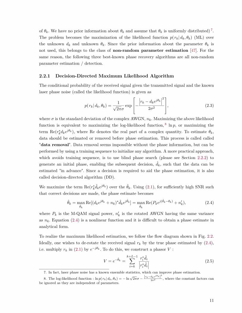
To realize the maximum likelihood estimation, we follow the flow diagram shown in Fig. 2.2.Ideally, one wishes to de-rotate the received signal rk by the true phase estimated by (2.4),i.e. multiply rk in (2.1) by e−jθk . To do this, we construct a phasor V :

V = e−θk =k+L−1∑i=k

r∗i di∣∣∣r∗i di∣∣∣ (2.5)

7. In fact, laser phase noise has a known ensemble statistics, which can improve phase estimation.

8. The log-likelihood function : ln p(rk| dk, θk) = − ln√

2πσ − |rk−dkejθk |2

2σ2 , where the constant factors canbe ignored as they are independent of parameters.

11

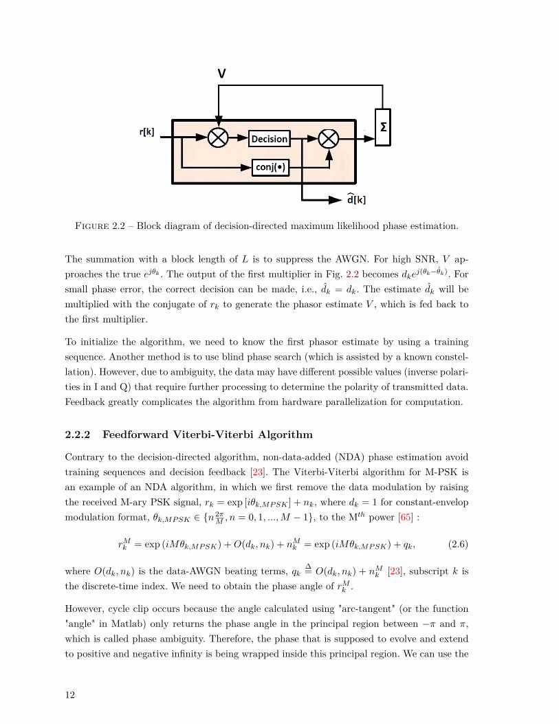
Figure 2.2 – Block diagram of decision-directed maximum likelihood phase estimation.

The summation with a block length of L is to suppress the AWGN. For high SNR, V ap-proaches the true ejθk . The output of the first multiplier in Fig. 2.2 becomes dkej(θk−θk). Forsmall phase error, the correct decision can be made, i.e., dk = dk. The estimate dk will bemultiplied with the conjugate of rk to generate the phasor estimate V , which is fed back tothe first multiplier.

To initialize the algorithm, we need to know the first phasor estimate by using a trainingsequence. Another method is to use blind phase search (which is assisted by a known constel-lation). However, due to ambiguity, the data may have different possible values (inverse polari-ties in I and Q) that require further processing to determine the polarity of transmitted data.Feedback greatly complicates the algorithm from hardware parallelization for computation.

2.2.2 Feedforward Viterbi-Viterbi Algorithm

Contrary to the decision-directed algorithm, non-data-added (NDA) phase estimation avoidtraining sequences and decision feedback [23]. The Viterbi-Viterbi algorithm for M-PSK isan example of an NDA algorithm, in which we first remove the data modulation by raisingthe received M-ary PSK signal, rk = exp [iθk,MPSK ] + nk, where dk = 1 for constant-envelopmodulation format, θk,MPSK ∈ {n2π

M , n = 0, 1, ...,M − 1}, to the Mth power [65] :

rMk = exp (iMθk,MPSK) +O(dk, nk) + nMk = exp (iMθk,MPSK) + qk, (2.6)

where O(dk, nk) is the data-AWGN beating terms, qk∆= O(dk, nk) + nMk [23], subscript k is

the discrete-time index. We need to obtain the phase angle of rMk .

However, cycle clip occurs because the angle calculated using "arc-tangent" (or the function"angle" in Matlab) only returns the phase angle in the principal region between −π and π,which is called phase ambiguity. Therefore, the phase that is supposed to evolve and extendto positive and negative infinity is being wrapped inside this principal region. We can use the

12

standard Matlab function "unwrap" to unwrap the phase 9, or use the algorithms mentionedin [23, 65]. We assume that qk is a small additive noise, the unwrapped phase becomes [65]

arg{rMk

}= Mθk,MPSK + n′k, (2.7)

where n′k is an one-dimensional noise To estimate θk, one uses a moving average (MA) filter 10

to remove the AWGN effect in coherent receivers, such that

θk,MPSK =k+L−1∑i=k

1M

arg{rMi

}, (2.8)

where L represents the MA filter length. In practice, for low OSNR (after long-haul trans-mission), the AWGN is large and causes more of the aforementioned phase ambiguities. Toreduce the probability of having more cycle slips, the moving average is performed before theangle function :

θk,MPSK = 1M

arg{k+L−1∑i=k

rMi

}, (2.9)

Finally, we apply the phase estimate to the complex field using e−jθk,MPSK and to the receivedsignal rk to remove the phase noise. The estimated data becomes

dk = rke−jθk,MPSK = dke

jθk,MPSK−jθk,MPSK + nke−jθk,MPSK . (2.10)

For perfect phase estimation, the estimated data is equal to the transmitted data.

Feedforward Viterbi-Viterbi Algorithm for MQAM

Figure 2.3 – Symbols classification used in Viterbi-Viterbi algorithm (modified for MQAM)in (a) Seimetz’s work [52] and (b) Gao et al.’s work [13] .

For M-QAM, the M-th power approach is not effective at every constellation point. For 16-QAM, Seimetz [52] classified the constellation points into two subgroups (Class I and II)

9. For implementation, phase recovery is a symbol-wise operation, and therefore the cycle-slip detectionand correction must be done symbol-wise, enhancing the hardware complexity due to parallelization.10. While a moving average filter is suboptimal (the Wiener filter is optimal [65] ), it is used for simplicity.

13

shown in Fig. 2.3. Only the symbols in the subgroup Class I, i.e., π4 +nπ2 , n = {0, 1, 2, 3}, willbe chosen for phase estimation, and the estimated phase noise for square M-QAM becomes

θIk,MQAM = 14 arg

k+NI−1∑i=k

r4i,I∣∣∣r4i,I

∣∣∣ , (2.11)

where θIk,MQAM is the estimated phase using the received symbols in Class I, rk,ClassI is thereceived signal falling into the subgroup Class I, NI is the number of Class I symbols used togenerate θIk,MQAM . Since only a subgroup of received signals is used, the algorithm is sensitiveto laser phase noise. Gao et al. [13] proposed a modified Mth power approach, by classifyingthe inner-ring symbols and the outer-ring symbols as Class I and Class III, respectively, anduse both classes for phase estimation :

θI,IIIk,MQAM = 14 arg

k+NI−1∑i=k

r4k,I∣∣∣r4k,I

∣∣∣ +W1

k+NIII−1∑i=k

r4k,III∣∣∣r4k,III

∣∣∣ , (2.12)

where θI,IIIk,MQAM is the estimated phase using the received symbols in both Class I and ClassIII, rk,III is the received signal falling into the subgroup Class III, NIII is the number of ClassIII symbols used to generate θIk,MQAM , W1 is a weighting coefficient which takes into accountthe fact that symbols in the outer ring have a higher OSNR and hence carrier phase estimatesfrom these symbols should be better than those from the inner ring. Moreover, Fatadin et al.[9] shifted the middle-ring symbols by ±19.5o in order to fully make use of all symbols forphase estimation :

θk,MQAM = θI,IIIk,MQAM +W2θIIk,MQAM , (2.13)

where θIIk,MQAM is the estimated phase corresponding to the middle ring,W2 is another weightcoefficient for the estimated phase using Class II received symbols.

2.3 Detection-based Method

The concept of the blind-phase search (BPS) [44] is to estimate the laser phase noise of thereceived signal, by making a choice between different (discrete, countable) phase candidatesthat can minimize the defined cost function. As the parameters are discrete, not a continuumof possible values, this problem belongs to the composite hypothesis testing in detectiontheory [47].

2.3.1 Feedforward Blind-Phase Search (BPS)

As shown in Fig. 2.4, the received signal after sampling, Yk, is first rotated by B test phaseangles ϕb by multiplying Yk with B phasors terms ejϕb , where

ϕb = b

B· π2 , b = {0, 1, ..., B − 1} . (2.14)

14

Note that, since square M-QAM has a π/2-rotational symmetry, the maximum range of thetest phase angles is π/2, meaning that these test phase angles cover only one quadrant on thecomplex plane. As the laser phase noise rotates the constellation of the transmitted square

Figure 2.4 – Block diagrams of feedforward blind phase search, reproduced from Fig. 4 in[44].

M-QAM symbols, the corrupted squared M-QAM symbols are no longer at their originalpositions. The interesting point of this blind phase search is that it makes use of the originalconstellation shape of squared M-QAM to undergo data-removal. The followings show thestep of BPS :

1. De-rotation using each test phase : De-rotate each received symbol by test phaseangles shown in Fig. 2.5.

2. Calculation of cost function : Calculate the cost function of the B de-rotated receivedsymbol. The cost function is defined as the Euclidean distance, dk,b, between the de-rotated receiver symbol and the original position of square M-QAM symbols, where kis the time index of the received symbols.

|dk,b|2 =∣∣∣Ykejϕb − Xk,b

∣∣∣2 , (2.15)

where Yk is the sampled received signal, Xk,b is the output of the decision device, whichis equal to one of the M-QAM symbol whose position is the closest to the rotatedreceived symbol.

15

3. Moving average : To reduce the impact of the ASE noise, one may use a movingaverage filter to estimate the Euclidean distances taken within a block of 2N+1 symbols,shown in the bottom part of Fig. 2.4.

4. Searching optimal test phase : There is only one test phase closest to the true phase,resulting in a minimum average Euclidean distance.

5. Compensation : The optimal phase is used to de-rotated the received symbol.

Figure 2.5 – B test phases in a quadrant. Background : 16-QAM with uncompensated phasenoise [44].

This blind phase search does not require phase unwrapping, since the estimation is doneon the complex plane (directly on the electric field). However, because of the π/2-rotationalsymmetry of square M-QAM, 4-fold ambiguity leads to a new problem : for example, when thephase noise passes from the first quadrant to the second quadrant, it will be misinterpretedas the phase angle in the first quadrant (the current phase value minus π/2). It is because, asaforementioned, the range of the test phase angles for PMS is only from zero to π/2 (coveringonly the first quandrant).

Due to the 4-fold ambiguity of the recovered phase in squared M-QAM, differential encodingwill be used to encode the first two bits of each symbol. For details, please refer to SectionIII in [44].

2.4 Parallelization and Pipelining

There are two practical problems in the implementation of DSP for optical communication.First, power consumption of CMOS chips increases linearly with clock frequency [[42], (3.10)],

16

and therefore increases with data rate ; DSP at lower clock speed provides power savings. Se-cond, the currently available ASICs and reconfigurable FPGA cannot process at Gbaud rates.Parallel processing and pipelining are required, which tremendously increases the effective li-newidth of lasers.

For parallel processing, the serial data is acquired in a time-interleaved manner into severalparallel channels having duplicate processing hardware [42]. This allows processing multipledata in parallel in a clock period. With time-interleaved parallelization, the receivedsymbols at Gbaud rates (symbol period Tsym ) are demultiplexed into P sub-GHz channelsfor DSP. For example, in Fig. 2.6, during the first round of time interleaving P symbols, r[k],r[k−1] , . . . , r[k−P +1] arrive at the input of the first, second, . . . , P th channel, respectively.Next, another P symbols, r[k + P ], r[k + P − 1], . . . , r[k + 1] follow, and the process willrepeat. Thus, the ith channel receives time-interleaved symbols r[k − i+ 1], r[k − P − i+ 1],r[k − 2P − i + 1], and so on, where i is the index of parallelization channels, taken from1 to P , where P is the number of parallelization. Two adjacent symbols in each channelhave a time separation of P × Tsym, instead of Tsym in serial processing. As a result, eachchannel perceives laser phase noise having a variance of 2π(P∆ν)Tsym, i.e., time-interleavedparallelization increases the effective laser linewidth by a factor of P .

Figure 2.6 – Implementation of decision-direct maximum likelihood estimation for a time-interleaved structure [75].

Even though ASIC design allows higher processing speed than FPGAs by circuit optimiza-tion, multipliers and lookup tables are unavoidable sources of latency. The throughput of an

17

algorithm simply cannot keep up with the input data rate (sampling rate) at each paralleli-zation channel. Pipelining must be introduced in order to increase the effective sampling rate[42]. For example, an algorithm usually consists of multipliers, slicers and lookup tables thatcannot be implemented within one clock cycle. Thus pipelining is required, in which delays(flip-flops [44] or so-called pipelining registers [42]) are added between individual operationsrequiring a clock cycle or less ; the immediate result of each operation is stored in registersfor subsequent manipulation.

2.5 Implementation of DDMLE

Decision-directed phase recovery (DD-PR) is the preferred solution for high baud rate, higher-density constellation systems. The serial DD-PR intrinsically contains one symbol delay onthe feedback path. To realize parallel DD-PR in ASIC or FPGA, however, the feedbackdelay is increased. To illustrate the effect of feedback delay in parallel DD-PR, we select thedecision-directed maximum likelihood estimation (DD-MLE).

For serial tracking, DD-MLE can be linearized as the following first-order discrete loop equa-tion [[15], (6)],

θk+1 = θk + U, (2.16)

where θk is the phase estimate, and U is the phase increment ; U is a function of the parametersof the moving average filter, laser phase noise variance and SNR. For parallel tracking withfeedback delay, as shown in Appendix D, (2.16) can be modified as

θk−i+1 = θk−D−i+1 + f

({θ, θk−D−i+1, d, n

∗1}), (2.17)

where

θ = [θ]m=k−D−P+1k−D , (2.18)

d = [dm]m=k−D−P+1k−D , (2.19)

n∗1 = [n∗1,m]m=k−D−P+1k−D (2.20)

where i is the parallelization channel index taking from 1 to P , D = P × d, d is the numberof pipelining registers in the closed loop, θ, d and n∗1 are vectors of true phases, transmittedsymbols and the AWGN, respectively, taking from k−D− P + 1 to k−D. The second termof right-hand side of (2.17) is the increment of the discrete loop equation, which is a functionof phase tracking error, transmitted symbols and the AWGN seen in each rail taking fromk − D − P + 1 to k − D. For higher parallelization levels (required to process Gbaud ratesin optical communications, e.g. P = 20 for 5 Gbaud signal and 250 MHz ASIC speed ), thefeedback delay of D symbols results in much higher phase error than that of serial tracking.For d > 1, the effect of the feedback delay dominates that of the moving average filter, and

18

therefore the introduction of feedback delay equivalently reduces loop bandwidth and phasemargin [15].

Fig. 2.6 shows that the implementation of DD-MLE has four pipelining registers in the closedloop [75], i.e., d = 4. The effect of the loop delay can be conceptually illustrated as in Fig. 2.7.The estimated phase is generated using (k-5P+1)th to (k-4P )th symbols. The compensation isapplied to the (k-P+1)th to kth received symbols, introducing a lag of approximately D = 4×P×Tsym seconds. Delayed phase noise compensation caused by pipelining registers on feedbackpath further increases phase error variance to approximately 2π(4P∆ν)Tsym, i.e., the effectivelaser linewidth further increases in the DD-MLE case by 4P . Pipelining delays are detrimentalto real-time feedback-delayed phase tracking at Gbaud-rate optical communications.

Figure 2.7 – Equivalence of implementation of DD-MLE with feedback delay.

2.6 Frequency Noise Power Spectrum Density

In this section, we will introduce three frequency ranges of frequency noise power spectraldensity (FN-PSD), which will be useful in Chapters 3 and 4. We will later see that phaserecovery depends on the FN-PSD level rather than laser linewidth. Thus, one may use theFN-PSD as a figure of merit instead of laser linewidth to understand the impact of the lasersources on the phase tracking. As shown in Fig. 2.8, we can divide the FN-PSD into threedifferent regions based on offline processing, parallel processing and non-ideal frequency offsetcompensation :

19

Figure 2.8 – Laser Frequency noise power spectral density.

– Above 100 MHz : This region is pertinent to all kinds of algorithms for theoreticalanalysis or offline processing that assume the absence of feedback delay in phase recoveryalgorithms.

– 10 MHz-100 MHz : This region affects the decision-directed phase recovery in thepresence of feedback delay for QAM signals. We will devote Chapter 3 to explain howTeraXion’s narrow-linewidth lasers can outperform the conventional laser sources dueto the frequency noise suppression in this frequency range.

– Below 1 MHz : The laser frequency noise in this region does not directly affect thephase tracking. However, any frequency tones in this region, depending on the amplitudeor frequency, could result in significant residual frequency offset using the conventionalfrequency offset compensation techniques. The large residual frequency offset may resultin phase tracking failure caused by the reduced bandwidth due to feedback delay. Wewill devote Chapter 4 to this problem.

2.7 Summary

In this chapter, we have revisited the three conventional phase recovery algorithms : Viterbi-Viterbi phase estimation, decision-directed maximum likelihood estimation and blind phasesearch.

For commercial DP-QPSK coherent systems, Viterbi-Viterbi phase estimation is used becauseof its simplicity and feedforward structure. For DP-16QAM, BPS is a good candidate. Ho-wever, BPS suffers from its high computational effort, as BPS calculates the error functions

20

for all the test phase candidates. Therefore, the modified Viterbi-Viterbi phase estimation ispreferred for 16-QAM in order to avoid feedback delay.

For 64-QAM or higher, the modified Viterbi-Viterbi phase estimation shows extra opticalsignal-to-noise ratio (OSNR) penalty due to amplitude discrimination and its stringent la-ser linewidth requirement. The BPS requires tremendous computational effort to providethe necessary phase resolution. DD-MLE requires the least computational effort and doesnot require amplitude discrimination, and this is typically used for 64-QAM experimentaldemonstrations with offline DSP [18, 43, 10, 76]. Nevertheless, feedback delay remains anobstacle to implement DD-PR in real-time [76].

21

Chapitre 3

Optically Filtered Laser

In this chapter, we will examine the performance of TeraXion’s narrow-linewidth laser sourcewith a decision-directed phase recovery algorithm as discussed in Section 2.5. We will discussthe operation of TeraXion’s novel lasers. We will discuss the experimental results of lasercharacterization, in which we extracted some physical parameters from the laser sources.For background on laser characterization, please refer to Appendix F. We will discuss therelationship between the laser frequency-noise power spectral density, parallelization leveland phase tracking bandwidth for 64 QAM using our heuristic approach. We will presentour experimental results for the system performance given by TeraXion’s lasers when usingparallel and pipelined phase tracking in a single-carrier 5 Gbaud 1 64-QAM back-to-backcoherent system.

3.1 Introduction

Implementation of real-time gigabaud optical coherent systems for single-carrier higher-levelmodulation formats such as 64-QAM depends heavily on phase tracking. For offline digitalsignal processing, decision-directed phase recovery (seen in Section 2.2.1) is performed at thesymbol rate and has the best performance and the least computational effort compared toother best-known algorithms. However, as the decision-directed phase recovery consists of afeedback proportional to parallelization level and pipelining delay, processing at the symbolrate is impractical in current electronics, as discussed in Section 2.4. This leads to the paucityof experiments demonstrating real-time phase tracking for 64- or higher QAM.

In the present chapter, we will experimentally investigate the improvement in system perfor-

1. We chose 5 Gbaud as our symbol rate because of the limitation of our MICRAM, the digital-to-analogconverter (DAC) in our laboratory. For 64-QAM generation, both I and Q require a 8-level signal, and thusthe DAC should provide at least 8 levels (3 bits) for a desired symbol rate. However, 8-level signals are moresusceptable to limited electrical bandwidth, requiring pre-distortion. As a result, 4 samples per symbols wereused to generated two 5 Gbaud 8-level electrical signals using our 20Gsa/s, 6 bit waveform generator (AWG)in MICRAM.

23

mance of TeraXion’s narrow-linewidth compared to conventional lasers, when we consider theuse of decision-directed maximum likelihood estimation in its implementation form shown inSection 2.5.

Contribution

In this chapter, we limit our scope for a back-to-back, single-polarization 2, single-carrier 5Gbaud 64-QAM heterodyne coherent system and consider the standard algorithm (paralleland pipelined DD-MLE) for phase tracking. We have made the following contributions :

1. We demonstrate how the laser linewidth is a poor predictor of DSP phase noise trackingefficiency.

2. We suggest the use of frequency noise power spectral density level to describe the impactof laser phase noise for real-time phase tracking with feedback delay, in contrary tonowadays offline experimental demonstrations in which the absence of feedback delay isassumed.

3. We experimentally show, for the first time, that TeraXion’s narrow-linewidth lasersgives BER improvement for 64 QAM. The use of a fiber Bragg grating suppresses thefrequency noise spectral level of contemporary narrow-linewidth semiconductor laserssuch as external cavity lasers (ECLs) or integrated tunable laser assemblies (ITLAs).

4. We found that the frequency noise of laser sources between 10 MHz and 100 MHzaffects the real-time decision-directed phase recovery as a result of reduction of trackingbandwidth due to hardware parallelization and pipelining. This result should hold aswell for higher symbol rates than those examined, as a higher symbol rate requireshigher parallelization in the current CMOS technology.

5. Compared to conventional laser sources, the TeraXion source permits greater paralleli-zation, e.g., increase from 16 to 20, to reduce the hardware processing rate from 312.5to 250 MHz.

3.2 TeraXion Novel Lasers

The following information about the laser product is provided by TeraXion.

In this project, we examined the performance of TeraXion’s Pure SpectrumTM -Tunable Nar-row Linewidth Lasers (PS-TNLs) in optical coherent communications. The PS-TNL is basedon an Integrated Tunable Laser Assembly (ITLA), with optical filtering of white frequencynoise by an ultra-narrowband multichannel fiber Bragg grating (FBG).

2. The experiment in this chapter was performed when the dual-polarization setup in our laboratory wasnot ready. In any case, this chapter is about optically-filtered phase noise, and one should only consider asingle-polarization scenario to rule out the polarization effect.

24

The optical filter produces 51 narrowband transmission peaks separated by 100 GHz [2]. Theinterleaved spectral responses present a narrow transmission peak (FWHM of 49 to 77 MHzfor all channels) at every 115 GHz from 191.4 to 196.6 THz, so that one peak can be thermallytuned to any frequency within this range. Fig. 3.1 shows the optical spectrum of the FBG

Figure 3.1 – Transmission spectrum of the FBG assembly. [2]

assembly including a polarization isolator and a polarizing tap isolator, measured betweenpoints A and B on Fig. 3.2. The ITLA has a measured linewidth of 10 kHz.

Figure 3.2 – Frequency locking schematic. TEC : thermoelectric cooler. [2]

The optical filtering of the laser spectrum is achieved by control of the laser carrier and thenarrow transmission peak of the FBG assembly. Fig. 3.2 illustrates the frequency lockingmechanism.

A dithering signal modulates the ITLA. The filtered signal is detected and sent to the control

25

electronics. Correction signals are generated to maintain alignment of the ITLA carrier fre-quency with a selected transmission peak. Both thermal tuning of the optical filter and ITLAcarrier frequency control is applied to correct the misalignment. Eventually slow variationsbecome less detrimental to phase estimation, whereas fast frequency fluctuation associatedto the wings of the laser spectrum falling outside of the narrowband transmission peak aresuppressed. The optical filtering scheme covers the entire C-band.

3.3 Laser Characterization

3.3.1 Experimental Results

For laser sources having pure Brownian phase noise (or equivalently white frequency noise), thelinewidth is defined as the 3-dB width of the Lorentzian field power spectral density (PSD) [7].To understand the interplay of phase noise reduction with phase tracking algorithms workingin a parallel architecture that we have discussed in Chapter 2.4, we must turn to the frequencynoise power spectral density (FN-PSD). Brownian phase noise leads to a flat FN-PSD. Acartoon of FN-PSD is given in Fig. 3.3 . The black solid line shows the mid-frequency band(from 10 to 100 MHz) dominated by Brownian phase noise, i.e., S∆f,BM = ∆ν/2π, where ∆νis the double of the original laser linewidth (because of the mixing in homodyne detection) ;it is constant over frequency. Conventionally, laser linewidth allows a quick quantificationof phase-error variance in coherent communication systems with Brownian phase noise forsystem performance analysis [40].

Figure 3.3 – Cartoon of frequency-noise power spectral density for a laser with active fre-quency noise reduction.

Additive white Gaussian noise (AWGN) results in a flat phase-noise power spectral density

26

(PN-PSD), or an upward sloping line in the FN-PSD. The AWGN FN-PSD, found in AppendixE, is

S∆f,AWGN (f)dB =[No

/(2A2

)]dB

+ 20log10f (3.1)

where No is the two-sided field PSD of white Gaussian noise (flat noise floor appeared in fieldPSD), and A is the amplitude of electric field of the receiver signal in the absence of noise.As illustrated in Fig. 3.3 (blue dotted, upward sloping line), the f2-FN AWGN measurementnoise dominates the filtered source at high frequencies (starting from hundreds of MHz).

Following the FBG filtering, the phase noise is no longer Brownian (the frequency noise iscolored), and therefore the simple parameterization by the linewidth is no longer valid, i.e., theFN-PSD is no longer flat at mid-frequencies. In particular, filtering by the ultra narrowbandFBG will create a downward slope in the FN-PSD shown in Fig. 3.3 (red dash).

As the ITLA laser linewidth is inappropriate to characterize the filtered ITLA, we must turnto other parameters. One definition of the suppression accorded by the noise filtering is tomeasure the reduction in FN-PSD at the point where measurement noise obscures laser phasenoise, as illustrated in Fig. 3.3 (green, dot-dashed lines). This parameterization, however,does not capture the frequency dependence of FN-PSD. The objective of this Chapter is toquantify the performance improvement for BER in the presence of parallelization in phasetracking. The level of parallelization will determine which frequency region will dominate.Greater parallelization level will lead to FN-PSD in the shaded region of Fig. 3.3 playing agreater role in overall performance.

TeraXion PS-TNLs provides two modes of operation :

1. a native mode, with the FBG at full transmission (without filtering) ;

2. a low-noise mode, with FBG filtering starting at 10 MHz.

The FN-PSD of the two operating modes of the PS-TNL are shown in Fig. 3.4 as measuredwith a self-homodyne coherent detection setup shown in Appendix F. Note that switchingto the low-noise mode of PS-TNLs reduces laser phase noise, but the phase-noise statisticsare changed so that the linewidth is no longer uniquely defined (refer to Appendix B). InFig. 3.4, the upper curve shows the FN-PSD of the free-running laser without FBG filtering,and the lower curve shows that optical filtering by an FBG suppresses the white FN by 4dB at frequencies above 50 MHz. The f2-FN (upward sloping) noise does not come from thelasers themselves, but mainly from the electrical noise of our coherent receiver (please referto Appendix E).

3.4 Insight from PSD

To maintain phase tracking, the phase-recovered symbols should fall well inside the decisionboundary. The decision boundary for 64-QAM is defined as the threshold angle beyond which

27

Figure 3.4 – FN-PSD of native mode (without FBG) and low-noise mode (with FBG).

erroneous decision will happen. This threshold angle is calculated as the distance between thecorner symbol of 64-QAM constellation and its closest symbol : 4.73 degrees (0.0263π radian).As previously mentioned, the feedback loop of parallel DD-PR introduces a delay betweenthe phase estimate and the current symbol, the phase tracking loop bandwidth for DSP inelectronics becomes Rs/(d× P ).

We propose a heuristic criterion to avoid loss of lock in phase tracking at moderate or highOSNR : the phase-noise increment between two adjacent symbols in each parallelization chan-nel should be smaller than a certain threshold which is a fraction of 64-QAM decision boun-dary. The phase-noise increment over the response time of the feedback loop Tloop is propor-tional to the root-mean square of its variance

0.0263π/K ≥

√4π2S

(f = Rs

Pd

)Tloop (3.2)

where Tloop is approximately equal to d× P × Tsym, K is a proportionality constant, whosevalue depends on the desired BER level at high OSNR. K is usually larger than unity to makethe threshold tighter in the presence of AWGN phase noise. Note that for phase tracking, weshould observe FN-PSD at operating frequency (loop bandwidth) f = Rs/(d × P ), which is

28

the corner frequency beyond which the feedback loop starts to lose tracking. (3.2) becomes

S∆f (f = RsPd

) ≤ (0.0263)2/K

4PdTsym(3.3)

Equation (3.3) tells us that when the parallelization level increases, the loop bandwidth ofparallel DD-MLE decreases, and the FN-PSD level has to be smaller by a factor of P in orderto maintain phase tracking. For filtered sources, the FN-PSD is shaped by the FBG filter witha corner frequency smaller than the phase-tracking loop bandwidth. The FN-PSD level, dueto the FBG suppression, is lower than that of the original laser within the loop bandwidth(as shown in the red-shaped region in Fig. 3.3, or 10-100 MHz in Fig. 3.4). Therefore filteredlasers can allow higher parallelization for a fixed number of pipelining delay elements on thefeedback path.

3.5 System Performance

3.5.1 Experimental Setup

In this section, we compare the bit-error rate (BER) performance of FBG-filtered lasers(low-noise mode) with that of unfiltered lasers (native mode) using parallel phase trackingin a time-interleaving structure as discussed in Section 2.4. Fig. 3.5 shows the experimentalsetup for single polarization back-to-back 5 Gbaud 64-QAM. Two separate PS-TNLs tunedat 1550 nm were used as transmitter and local oscillator sources. To examine the effect ofFBG filtering, two different measurements were taken :

1. both sources in native mode ;

2. both sources in low-noise mode.

A 20-GSa/s, 6-bit arbitrary waveform generator (AWG) operating at 4 samples per symbolwas used to generate two 5 Gbaud 8-level electrical signals. Data was a repeated sequenceof 98304 bits (limited by AWG memory) taken from a pseudorandom bit sequence with aword length of 31, driving the in-phase/quadrature (IQ) modulator. Wiener-Hopf-based [48]predistortion was applied to compensate for RF components and the imperfect linear gain ofthe power amplifier in the transmitter.

A combination of variable optical attenuator and EDFA was used to adjust the receivedOSNR. To maintain the integrated coherent receiver at its optimum operating point, thereceived optical power was fixed at -8 dBm and the local oscillator power was set to 13.8dBm. The coherently detected signal was sampled by the real time oscilloscope at 80 Gsa/swith 30-GHz electrical bandwidth. The captured samples were then retimed and resampledto one sample per symbol for the subsequent DSP.

29

Figure 3.5 – Top : experimental setup of back-to-back 5-Gbaud 64-QAM. Right bottom :Recovered 64 QAM constellation without parallelization at OSNR = 28 dB (BER= 6e-5).IQ mod : In-phase/Quadrature modulator, AWG : Arbitrary waveform generator, PM fiber :Polarization maintaining fiber, VOA : variable optical attenuator, OBPF : optical bandpassfilter, PC : polarization controller. Coh. Rx. : Coherent Receiver. RTO : Real time oscilloscope.EDFA : Erbium doped fiber amplifier.

3.5.2 Offline DSP

A non-data-aided fast Fourier transform-based frequency offset compensation (NDA-FFT-FOC) [53] was performed in a block-wise fashion over 30,000 symbols, to coarsely remove largefrequency offset (in GHz) between the two lasers at transmitter and at receiver. We appliedtraining-sequence-based Wiener-Hopf-based decision-directed equalizer (WH-DD-EQ) with 31taps [48]. Fine NDA-FFT-FOC was performed to further remove the effect of frequency offsetdynamics [69]. The serial data was demultiplexed into P channels, where P was varied from8 to 30 to observe the performance of different levels of parallelization (recall that the totalnumber of symbol delays due to the feedback loop is approximately P × d).

Blind phase search (BPS)-based pre-rotation [69] was used to obtain the initial phase of thefirst symbol of each channel. Subsequently, parallel DD-MLE (see Section 2.4) was used forphase recovery, incurring a pipelining delay of four [75]. The P channels were then recombinedinto a single data stream. We again applied 31-tap WH-DD-EQ [48] to further equalize withthe more reliable decisions following phase recovery. Finally, hard decision was performed onI and Q individually, and we counted errors. BER was estimated over 7 114 200 bits for eachOSNR value, which allows reliable estimation down to BER = 5.6e-5.

30

3.5.3 Results

In Fig. 3.6 we present BER versus OSNR results for native mode (square markers) andlow-noise mode (circle markers). For serial data processing (solid curves), the two sourcesoffer similar performance. For parallel DD-PR with P parallelization level and d pipeliningregisters on feedback path, the processing rate of each channel becomes Rs/P , leading tolarger phase excursions, where Rs is the optical baud rate. The feedback delay due to the dpipelining registers further reduces the loop bandwidth to approximately Rs/P/d, as discussedin Section 2.4. Hence, in Fig. 3.6, parallel processing leads to an increase in BER, but theFEC threshold (defined at BER = 1e-3) is still respected. For 12 parallel rails (dashed curves)and 24 rails (dotted curves) we see a reduced BER floor for the low noise mode.

Figure 3.6 – BER versus OSNR for native and low-noise mode of PS-TNLs for serial andparallel phase tracking (d = 4) with P = 12 and P = 24.

With FBG noise suppression, the phase tracking error decreases, improving BER. Note thatthe value for the curve P = 24 at OSNR = 28 dB is unexpectedly high. It is due to the fre-quency instability of the TeraXion laser source 3 We swept parallelization levels P , determined

3. The TeraXion source requries an error signal to lock the CW center frequency within the passband ofthe FBG filter. This error signal was sinusoidal originally at 75 kHz, and this frequency exceeds the bandwidthof the parallel DD-PR as explained in Chapter 4, and therefore extra effort in tracking and compensating the

31

BER and calculated the OSNR penalty at BER = 1e-3 for each level as shown in Fig. 3.7. Asecond axis is plotted across the top of Fig. 3.7 indicating the bandwidth of the phase trackingloop for the given parallelization level. The shaded area indicates where the phase trackingbandwidth falls within the noise-suppression bandwidth of the low-noise mode (with FBGnoise suppression). This area is determined by Fig. 3.4 where the low-noise-mode FN-PSDfalls below the native-mode FN-PSD. We see clearly that the low-noise mode improves theBER compared to the native mode within the shaded area.

For P = 8 and 12, corresponding to phase tracking loop bandwidth of 156.25 MHz and104.17 MHz, respectively, the low-noise mode cannot provide significant improvement. In thisfrequency region, the FN-PSD is dominated by the f2 frequency noise (i.e., white phase noise,shown in Appendix E). As shown in Fig. 3.4, the f2 frequency noise is visible in the linearlyincreasing logarithmic FN-PSD above 70 MHz. For higher parallelization, the phase trackingeffective loop bandwidth decreases, entering a band where the f2 frequency noise level of thecoherent receiver is lower than the white frequency noise level of the native mode (unfilteredlaser)

The frequency noise of laser sources between 10 MHz and 100 MHz affects the real-timedecision-directed phase recovery for 64-QAM at the symbol rate (5 Gbaud) examined. Atthis symbol rate, the tracking bandwidth due to hardware parallelization and pipelining fallswithin the noise suppression band for a wide range of parallelization levels (above 12). Thisconclusion should hold for higher symbol rates as well, as higher symbol rates require higherparallelization level, reducing the tracking bandwidth. The low-noise mode shows a 2 dBimprovement over the native mode for P > 24. When using the native mode, parallel DD-PReven fails for P > 26 while FBG filtering allows the break down point to extend up to P =30.

Fig. 3.8(a) and Fig. 3.8(b) shows the recovered constellation diagrams of native mode andlow-noise mode, respectively, for P = 26 at OSNR = 32 dB. Fig. 3.8(a) shows the rotationof symbols at the outermost ring, leading to high bit error rate (BER = 1e-3). With FBGsuppression, the FN-PSD is lowered, helping the reduction of rotation of symbols at theoutermost ring (BER = 4e-4) as shown in Fig. 3.8(b). As mentioned in Chapter 2, powerconsumption of CMOS chips increases linearly with clock frequency [42], we compare P = 16for native mode with P = 20 for low-noise mode for the same OSNR penalty in Fig. 3.7. Thedecrease of processing rate from 312.5 MHz to 250 MHz allows a 6.3 % reduction in powerconsumption for performing phase recovery in hardware (Appendix C).

frequency offset dynamics was performed before the parallel DD-PR, which was not shown in this thesis. Theunexpectedly large BER value appeared on the curve P = 24 at OSNR = 28 dB was caused by the failureof compensating an occasionally extreme frequency offset dynamics (even higher than 75 kHz) caused by thefrequency control of the laser.

32

Figure 3.7 – OSNR penalty for back-to-back 5 Gbaud 64-QAM with d = 4 versus paralleli-zation (lower axis) and versus bandwidth of phase tracking loop (upper axis) for both nativemode and low-noise mode. Shaded area is the noise suppression band, i.e., in Fig. 3.4 wherelow-noise FN-PSD falls below native FN-PSD.

Figure 3.8 – Constellations over 30 000 symbols, P = 26, d = 4, OSNR = 32 dB for (a)native mode (BER = 1e-3) and (b) low-noise mode (BER = 4e-4).

3.6 Conclusions

In this chapter, we have seen that laser linewidth is no longer appropriate to quantify laserphase noise. Frequency noise power spectral density levels are better descriptors of the impactof laser phase noise for real-time phase tracking with feedback delay, in contrary to nowadays

33

offline experimental demonstrations in which the absence of feedback delay is assumed. We ex-perimentally showed the system performance given by TeraXion’s narrow-linewidth lasers onparallel and pipelined DD-MLE in a single-carrier 5 Gbaud 64-QAM back-to-back heterodynecoherent system. Using a FBG filter (an optical approach) further suppresses the frequencynoise spectral level of contemporary narrow-linewidth semiconductor lasers such as ECL orITLA. We found that the frequency noise of laser sources between 10 MHz and 100 MHzaffects the real-time decision-directed phase recovery. For parallelization level higher than 24,TeraXion’s narrow-linewidth lasers show more than 2 dB improvement in OSNR penalty com-pared to that of conventional lasers. For the same OSNR penalty, the optically-filtered laserpermits greater parallelization, e.g., increase from 16 to 20, to reduce the hardware processingrate from 312.5 to 250 MHz.

34

Chapitre 4

Impact of Sinusoidal PhaseModulation on Phase Tracking

In Chapter 2, we found that real-time implementation of DSP at Gbaud rates requires hard-ware parallelization to increase the effective sampling rate of each sub-data rate parallelchannel and to reduce power consumption [42]. In Chapter 3, we have seen that the frequencynoise of laser sources between 10 MHz and 100 MHz affects the real-time decision-directedphase recovery as a result of reduction of tracking bandwidth due to hardware parallelizationand pipelining. In Chapter 3 we assumed no frequency offset (or after a perfect frequency off-set compensation). For systems employing dense constellations, such as 64-QAM, the phasemargin (the allowable maximum amount of phase rotation without tracking loss) is greatlyreduced compared to the commercially available 16-QAM. A residual frequency offset willgive a phase rotation larger than the pure Wiener phase noise of laser sources. Because ofthe bandwidth-reduced phase tracking, we may foresee difficulties in implementing 64-QAMcoherent receivers. Nevertheless, the impact of the non-ideal frequency offset compensationon the real-time phase tracking with feedback loop has not been investigated. This chapteris devoted to explore the phase tracking failure caused by the frequency components of lasersources below 10 MHz.

We will revisit a best-known, standard frequency offset compensation algorithm, followed by adetailed explanation of the impact of residual frequency offset on real-time phase tracking. Wewill present our experimental results on the effect of sinusoidal laser phase noise on paralleldecision-directed maximum likelihood estimation (DD-MLE) with four pipelining delays onits feedback path [75] in a single-polarization 1 single-carrier 5 Gbaud 64-QAM system. Weuse simulation to parameterize the range of frequency modulation-amplitude and frequency-

1. We only used a single-polarization experimental setup because the dual-polarization setup was not readyby the time of the publication related to this chapter. Moreover, this chapter is only devoted to the impact ofsinusoidal phase modulation on phase tracking, and therefore this single-polarization back-to-back experimentisolated the phase noise effect from polarization impairment.

35

modulation frequency that lead to tracking failure. Taking into account the effects of theconventional frequency offset estimation algorithm as well as equalization, we examine phasetracking performance as a function of parallelization level.

4.1 Introduction

Frequency offset between transmit and receive lasers can be interpreted as a long-term linearphase change. If not correctly compensated this offset can disrupt phase tracking. Non-data-aided fast-Fourier-transform (NDA-FFT)-based, also called periodogram-based, frequency off-set compensation (FOC) [53] is typically preferred over the less practical data-aided phase-locked loop (PLL) approach [49, 76]. NDA-FFT gives one single frequency-offset estimate 2

over the data block of concern, and its feedforward structure facilitates hardware implemen-tation. The PLL allows tracking 3 of frequency-offset dynamics but is impractical due to largefeedback delay (which requires the feedback of phase estimates to the FOC stage) [49, 76],and thus can only be used for offline demonstrations, but not for real-time implementations.The state-of-the-art FOC algorithms for QPSK and 16-QAM were designed to compensatea large frequency offset. The small residual (or uncompensated) frequency offset is assumedto be canceled in the subsequent feedforward phase recovery like (modified) Viterbi-Viterbialgorithm in Section 2.2.2 or blind phase search in Section 2.3.1. However, the small residualfrequency offset may exceed the phase margin of phase tracking for denser constellations suchas 64-QAM.

For offline serial phase tracking [43, 76, 18], residual frequency offset or fast frequency mo-dulation (FM) does not affect decision-directed phase tracking (DD-PR) as the bandwidthof the tracking loop exceeds that of phase variation. For real-time implementation, paralleli-zation and pipelining introduce a large delay on the feedback path of DD-PR, reducing thebandwidth of parallel phase tracking as mentioned in Chapter 2. Residual frequency offset orfast FM creates a phase rotation that causes tracking failure for parallel phase recovery. Inthe presence of sinusoidal FM, the varying phase spoofs the NDA-FFT-based FOC, leadingto sporadic phase tracking failure. Data blocks falling in certain sections of the sinusoidalcycle with fast phase variation, i.e. near sinusoidal maxima, are prone to tracking failure (tobe explained later).

Sinusoidal frequency modulation may be intentional for control purposes, or incidental dueto electronics and environmental fluctuations. For instance, parasitic sine tones can originatein switching power supplies and power converters driving the laser diode. Kuschnerov et al.[30] experimentally investigated the impact of mechanical vibrations using sinusoidal FM in alaser source. That study examined QPSK with Viterbi-Viterbi (V-V) phase tracking algorithm

2. NDA-FFT belongs to parameter estimation. Please refer to Appendix A.3. The PLL for frequency offset tracking does not require the temporal dynamics of the frequency offset.

Please refer to Appendix A.

36

as well as 16-QAM with blind phase search. They showed that the FM amplitude and FMfrequency should be smaller than 120 MHz and 35 MHz, respectively, for QPSK and 16-QAMfor penalty to be negligible.

Gianni et al. [17] analyzed 10 GBaud QPSK via simulation a parallel second-order DPLL(digital phase locked loop) followed by V-V algorithm in the presence of frequency modulation,extending [16] to 16-QAM by adding one more BPS stage. Qiu et al [49] recently proposedusing shorter data blocks for QPSK and 16-QAM for frequency offset tracking to compensaterapid drift. Their approach is only applicable to offline processing, as they did not take intoaccount feedback delay in parallel DPLL. There has been no report to date, to the best of ourknowledge, of the impact of FM in 64-QAM, where phase-error tolerance is greatly reducedvis-à-vis 16-QAM.

Contribution

We will investigate the impact of the sine tones of laser sources on parallel and pipelineddecision-directed phase recovery (maximum likelihood estimation) in digital coherent recei-vers, as a result of residual frequency offset uncompensated by the conventional frequencyoffset compensation algorithm (NDA-FFT)[53]. Experimentally, we limit our investigationto a back-to-back, single-polarization, single-carrier 5 Gbaud 64-QAM heterodyne coherentsystem as shown in Fig. 4.1. We have made the following contributions in this chapter :

Figure 4.1 – Block diagram of a single-polarization, single-carrier coherent system.

1. We pointed out, for the first time, that the standard NDA-FFT FOC algorithm couldbe the cause of real-time phase tracking failure for 64-QAM in the presence of sine tonesin laser sources, whose frequencies lie on the range below 1 MHz, shown in Fig. 2.8.

2. We investigated, for the first time, the ranges of the FM amplitude and FM frequencyof laser sources to avoid real-time phase tracking failure using simulation.

37

4.2 Frequency Offset Compensation Algorithm

In this section, we will briefly introduce the frequency offset compensation algorithm that wewill consider in this chapter.

Selmi et al., first applied the non-data-aided fast-Fourier-transform (NDA-FFT) method, alsocalled periodogram-based or FFT-maximization-based method, for frequency offset compen-sation (FOC) [53]. The frequency offset ∆fFO is estimated by

∆fFO = 14 max

f

{fft(r4[k]

)}, (4.1)

where fft denotes the fast Fourier transform over a certain block size LFFT . r[k] is the receivedsymbol, where k is the time index taking over LFFT . Therefore, frequency offset estimate∆fFO is assumed to be constant over every LFFT symbols. This frequency offset estimationbecomes inaccurate when the frequency offset dynamics is fast within the block. Practically,to reduce the computational power, k is taken for every symbol duration Tsym rather thanthe sample duration because the sampling rate of a system is usually higher than the symbolrate.

NDA-FFT FOC raises the received signal (which includes a true frequency offset ∆fFO ) bya power of four to remove the symmetry of QAM signals (to avoid ambiguities in frequencyoffset estimation), and then to find out the frequency component, f , such that the phasorexp(j2πfkTsym) results in a maximum correlation with the 4th-power received signal, r4[k],over a block length (a time duration). This is equivalent to a FFT operation. In the FFTspectrum, the maximum peak refers to a frequency value close to 4×∆fLO . This value isthen divided by 4 to obtain the frequency offset estimate, ∆fFO. Then we multiply thereceived signal r[k] symbol-by-symbol by exp(−j2π∆fFOkTsym).

4.3 Effect of Residual frequency offset

After having discussed the NDA-FFT FOC algorithm, this section will explain in detail theimpact of residual frequency offset on real-time phase recovery with feedback with the aidof our simulation. First of all, we parameterize the sine tones in our laser sources (in bothtransmitter and receiver) with sinusoidal FM modulation at frequency fm and peak-to-peakFM amplitude of App. The electric field A(t) can be expressed as

A (t) = exp{j2πfct+ j

App2fm

cos (2πfmt) + jθLPN (t)}

(4.2)

where fc is the laser carrier frequency and θLPN is the laser phase noise.

In order to explain the effect of residual frequency offset on the parallel and pipelined maxi-mum likelihood phase estimation, only the temporal change of laser phase noise, excluding

38

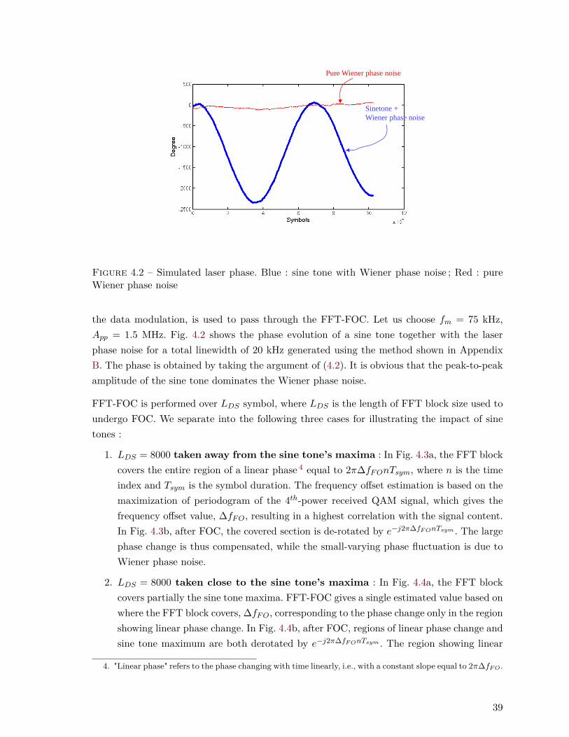
1

Pure Wiener phase noise

Sinetone +

Wiener phase noise

Figure 4.2 – Simulated laser phase. Blue : sine tone with Wiener phase noise ; Red : pureWiener phase noise

the data modulation, is used to pass through the FFT-FOC. Let us choose fm = 75 kHz,App = 1.5 MHz. Fig. 4.2 shows the phase evolution of a sine tone together with the laserphase noise for a total linewidth of 20 kHz generated using the method shown in AppendixB. The phase is obtained by taking the argument of (4.2). It is obvious that the peak-to-peakamplitude of the sine tone dominates the Wiener phase noise.

FFT-FOC is performed over LDS symbol, where LDS is the length of FFT block size used toundergo FOC. We separate into the following three cases for illustrating the impact of sinetones :

1. LDS = 8000 taken away from the sine tone’s maxima : In Fig. 4.3a, the FFT blockcovers the entire region of a linear phase 4 equal to 2π∆fFOnTsym, where n is the timeindex and Tsym is the symbol duration. The frequency offset estimation is based on themaximization of periodogram of the 4th-power received QAM signal, which gives thefrequency offset value, ∆fFO, resulting in a highest correlation with the signal content.In Fig. 4.3b, after FOC, the covered section is de-rotated by e−j2π∆fFOnTsym . The largephase change is thus compensated, while the small-varying phase fluctuation is due toWiener phase noise.

2. LDS = 8000 taken close to the sine tone’s maxima : In Fig. 4.4a, the FFT blockcovers partially the sine tone maxima. FFT-FOC gives a single estimated value based onwhere the FFT block covers, ∆fFO, corresponding to the phase change only in the regionshowing linear phase change. In Fig. 4.4b, after FOC, regions of linear phase change andsine tone maximum are both derotated by e−j2π∆fFOnTsym . The region showing linear

4. "Linear phase" refers to the phase changing with time linearly, i.e., with a constant slope equal to 2π∆fFO.

39

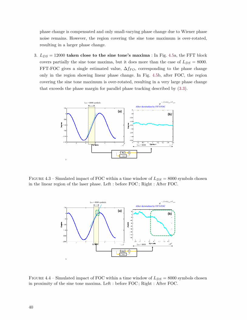
phase change is compensated and only small-varying phase change due to Wiener phasenoise remains. However, the region covering the sine tone maximum is over-rotated,resulting in a larger phase change.

3. LDS = 12000 taken close to the sine tone’s maxima : In Fig. 4.5a, the FFT blockcovers partially the sine tone maxima, but it does more than the case of LDS = 8000.FFT-FOC gives a single estimated value, ∆fFO, corresponding to the phase changeonly in the region showing linear phase change. In Fig. 4.5b, after FOC, the regioncovering the sine tone maximum is over-rotated, resulting in a very large phase changethat exceeds the phase margin for parallel phase tracking described by (3.3).

2

After derotation by FFT-FOC

2F O sym

j f nT

e LDS = 8000 symbols

LDS = 8000

(a) (b)

Figure 4.3 – Simulated impact of FOC within a time window of LDS = 8000 symbols chosenin the linear region of the laser phase. Left : before FOC ; Right : After FOC.

3

LDS = 8000 symbols

After derotation by FFT-FOC

2F O sym

j f nT

e

LDS = 8000

(a) (b)

Figure 4.4 – Simulated impact of FOC within a time window of LDS = 8000 symbols chosenin proximity of the sine tone maxima. Left : before FOC ; Right : After FOC.

40

4

LDS = 12000 symbols

2F O sym

j f nT

e

After derotation by FFT-FOC

LDS = 12000

(a) (b)

Figure 4.5 – Simulated impact of FOC within a time window of LDS = 12000 symbols chosenin proximity of the sine tone maxima. Left : before FOC ; Right : After FOC.

Figure 4.6 – Frequency noise PSD of our laser under test (blue : white noise filtered ITLA).Source : TeraXion PS-TNL specification.

4.4 System Perfomance

4.4.1 Experimental Setup

The source provided by TeraXion had three settings

41

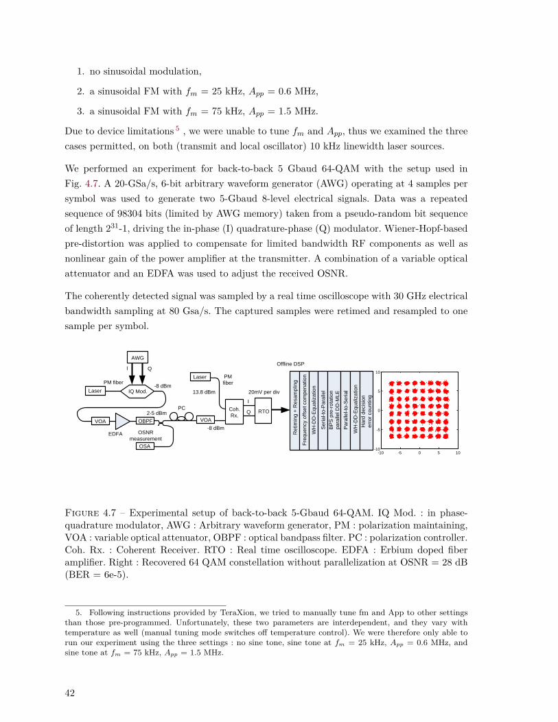
1. no sinusoidal modulation,

2. a sinusoidal FM with fm = 25 kHz, App = 0.6 MHz,

3. a sinusoidal FM with fm = 75 kHz, App = 1.5 MHz.

Due to device limitations 5 , we were unable to tune fm and App, thus we examined the threecases permitted, on both (transmit and local oscillator) 10 kHz linewidth laser sources.

We performed an experiment for back-to-back 5 Gbaud 64-QAM with the setup used inFig. 4.7. A 20-GSa/s, 6-bit arbitrary waveform generator (AWG) operating at 4 samples persymbol was used to generate two 5-Gbaud 8-level electrical signals. Data was a repeatedsequence of 98304 bits (limited by AWG memory) taken from a pseudo-random bit sequenceof length 231-1, driving the in-phase (I) quadrature-phase (Q) modulator. Wiener-Hopf-basedpre-distortion was applied to compensate for limited bandwidth RF components as well asnonlinear gain of the power amplifier at the transmitter. A combination of a variable opticalattenuator and an EDFA was used to adjust the received OSNR.

The coherently detected signal was sampled by a real time oscilloscope with 30 GHz electricalbandwidth sampling at 80 Gsa/s. The captured samples were retimed and resampled to onesample per symbol.

PM fiber

Laser IQ Mod.

AWG

VOA

EDFA

OBPF

PC

VOA

Coh.

Rx.

Laser

I

Q RTO

Offline DSP

-8 dBm

13.8 dBm

PM

fiber

20mV per div

OSA

OSNR

measurement

I Q

-8 dBm

2-5 dBm

Re

tim

ing

+ R

esa

mp

ling

Fre

qu

en

cy o

ffse

t co

mp

en

atio

n

WH

-DD

-Eq

ua

liza

tio

n

Se

ria

l-to

-Pa

ralle

l

BP

S p

re-r

ota

tio

n

pa

ralle

l D

D-M

LE

Pa

ralle

l-to

-Se

ria

l

WH

-DD

-Eq

ua

liza

tio

n

Ha

rd d

ecis

ion

err

or

co

un

tin

g

-10 -5 0 5 10-10

-5

0

5

10

Figure 4.7 – Experimental setup of back-to-back 5-Gbaud 64-QAM. IQ Mod. : in phase-quadrature modulator, AWG : Arbitrary waveform generator, PM : polarization maintaining,VOA : variable optical attenuator, OBPF : optical bandpass filter. PC : polarization controller.Coh. Rx. : Coherent Receiver. RTO : Real time oscilloscope. EDFA : Erbium doped fiberamplifier. Right : Recovered 64 QAM constellation without parallelization at OSNR = 28 dB(BER = 6e-5).

5. Following instructions provided by TeraXion, we tried to manually tune fm and App to other settingsthan those pre-programmed. Unfortunately, these two parameters are interdependent, and they vary withtemperature as well (manual tuning mode switches off temperature control). We were therefore only able torun our experiment using the three settings : no sine tone, sine tone at fm = 25 kHz, App = 0.6 MHz, andsine tone at fm = 75 kHz, App = 1.5 MHz.

42

4.4.2 Offline DSP

To investigate the impact of block length on FO estimation, NDA-FFT-FOC [53] with zeropadding (to guarantee a fixed FFT resolution) was performed repeatedly over data segmentsof LDS symbols, where LDS (length of data segment) = 4k, 6k, 8k 10k and 12k. For QPSK and16-QAM, the transmitter and receiver limitations are not too stringent and equalization maynot be required [18, 4] . However, for 64-QAM, equalization becomes necessary to achievea clear constellation and good bit-error rate (BER). We employed the statically optimalequalization (compared to adaptive equalization [76, 18] ), in the form of a Wiener-Hopf-based decision-directed equalizer (WH-DD-EQ) with 31 taps (refer to Section 3.5.2). TheWH-DD-EQ was updated by the same data segment of LDS symbols at the output of NDA-FFT- FOC.

The serial data was demultiplexed into P channels, where P was varied among 4, 6, 8, 10and 12 to observe the performance of different levels of parallelization. 64-QAM is much moresensitive to initial phase offset estimation than that for 16-QAM or QPSK when using DD-phase tracking. To solve this problem, BPS-based pre-rotation (in Section 2.3.1) was usedto obtain a good initial phase offset estimate at the first symbol in each parallel channel.Subsequently, parallel DD-MLE incurring four pipelining delays was used for phase recovery.The total delay is 4P , the product of pipelining delays and parallelization. The P channels werethen recombined into a single data stream. We again applied 31-tap WH-DD-EQ to furtherequalize with the more reliable decisions following phase recovery. Finally, hard decisions wereperformed for I and Q individually, and we counted errors. At each OSNR, 7114200 bits wereexamined, allowing reliable BER estimation down to 5.6e-5.

4.4.3 Results

The results of BER versus OSNR of parallel DD-MLE were compared with that of serial DD-MLE to obtain the OSNR penalty at BER = 1e-3. Fig. 4.8 shows the experimental OSNRpenalty versus different levels of parallelization, P . Each curve corresponds to a differentlength of data segment LDS for performing NDA-FFT-FOC and WH-DD-EQ. From Fig. 4.8,we can understand :

– Fixed P and smaller LDS : smaller LDS for NDA-FFT-FOC to reduce the fast varyingphase change due to the sine tone, but leads to an inadequate number of symbols fortraining the equalizer.

– Fixed P and larger LDS : a larger LDS results in a lower OSNR penalty as moresymbols can be used to train the WH-based equalizer for better channel estimation.Equalization does not show further improvement for LDS > 12k.

– Fixed LDS and smaller P : For P smaller than 8, OSNR penalty increases as Pdecreases, because smaller P leads to insufficient moving average in the parallel imple-

43

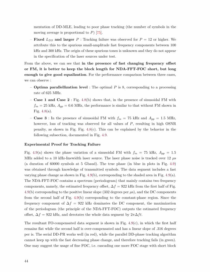
mentation of DD-MLE, leading to poor phase tracking (the number of symbols in themoving average is proportional to P ) [75].

– Fixed LDS and larger P : Tracking failure was observed for P = 12 or higher. Weattribute this to the spurious small-amplitude fast frequency components between 100kHz and 300 kHz. The origin of these spurious tones is unknown and they do not appearin the specification of the laser sources under test.

From the above, we can see that in the presence of fast changing frequency offsetor FM, it is better to keep the block length for NDA-FFT-FOC short, but longenough to give good equalization. For the performance comparison between three cases,we can observe :

– Optima parallellization level : The optimal P is 8, corresponding to a processingrate of 625 MHz.

– Case 1 and Case 2 : Fig. 4.8(b) shows that, in the presence of sinusoidal FM withfm = 25 kHz, App = 0.6 MHz, the performance is similar to that without FM shown inFig. 4.8(a).

– Case 3 : In the presence of sinusoidal FM with fm = 75 kHz and App = 1.5 MHz,however, loss of tracking was observed for all values of P , resulting in high OSNRpenalty, as shown in Fig. Fig. 4.8(c). This can be explained by the behavior in thefollowing subsection, documented in Fig. 4.9.

Experimental Proof for Tracking Failure

Fig. 4.9(a) shows the phase variation of a sinusoidal FM with fm = 75 kHz, App = 1.5MHz added to a 10 kHz-linewidth laser source. The laser phase noise is tracked over 12 µs(a duration of 60000 symbols at 5 Gbaud). The true phase (in blue in plots in Fig. 4.9)was obtained through knowledge of transmitted symbols. The data segment includes a fastvarying phase change as shown in Fig. 4.9(b), corresponding to the shaded area in Fig. 4.9(a).The NDA-FFT-FOC contains a spectrum (periodogram) that mainly contains two frequencycomponents, namely, the estimated frequency offset, ∆f = 922 kHz from the first half of Fig.4.9(b) corresponding to the positive linear slope (332 degrees per µs), and the DC componentsfrom the second half of Fig. 4.9(b) corresponding to the constant-phase region. Since thefrequency component of ∆f = 922 kHz dominates the DC component, the maximizationof the periodogram (the principle of the NDA-FFT-FOC) outputs the estimated frequencyoffset, ∆f = 922 kHz, and derotates the whole data segment by 2π∆ft.

The resultant FO-compensated data segment is shown in Fig. 4.9(c), in which the first halfremains flat while the second half is over-compensated and has a linear slope of .316 degreesper is. The serial DD-PR works well (in red), while the parallel DD-phase tracking algorithmcannot keep up with the fast decreasing phase change, and therefore tracking fails (in green).One may suggest the usage of fine FOC, i.e. cascading one more FOC stage with short block

44

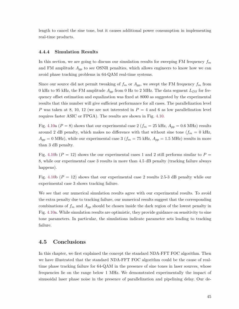
length to cancel the sine tone, but it causes additional power consumption in implementingreal-time products.

4.4.4 Simulation Results

In this section, we are going to discuss our simulation results for sweeping FM frequency fmand FM amplitude App to see OSNR penalties, which allows engineers to know how we canavoid phase tracking problems in 64-QAM real-time systems.

Since our source did not permit tweaking of fm or App, we swept the FM frequency fm from0 kHz to 95 kHz, the FM amplitude App from 0 Hz to 2 MHz. The data segment LDS for fre-quency offset estimation and equalization was fixed at 8000 as suggested by the experimentalresults that this number will give sufficient performance for all cases. The parallelization levelP was taken at 8, 10, 12 (we are not interested in P = 4 and 6 as low parallelization levelrequires faster ASIC or FPGA). The results are shown in Fig. 4.10.

Fig. 4.10a (P = 8) shows that our experimental case 2 (fm = 25 kHz, App = 0.6 MHz) resultsaround 2 dB penalty, which makes no difference with that without sine tone (fm = 0 kHz,App = 0 MHz), while our experimental case 3 (fm = 75 kHz, App = 1.5 MHz) results in morethan 3 dB penalty.

Fig. 4.10b (P = 12) shows the our experimental cases 1 and 2 still performs similar to P =8, while our experimental case 3 results in more than 4.5 dB penalty (tracking failure alwayshappens).

Fig. 4.10b (P = 12) shows that our experimental case 2 results 2.5-3 dB penalty while ourexperimental case 3 shows tracking failure.

We see that our numerical simulation results agree with our experimental results. To avoidthe extra penalty due to tracking failure, our numerical results suggest that the correspondingcombinations of fm and App should be chosen inside the dark region of the lowest penalty inFig. 4.10a. While simulation results are optimistic, they provide guidance on sensitivity to sinetone parameters. In particular, the simulations indicate parameter sets leading to trackingfailure.

4.5 Conclusions

In this chapter, we first explained the concept the standard NDA-FFT FOC algorithm. Thenwe have illustrated that the standard NDA-FFT FOC algorithm could be the cause of real-time phase tracking failure for 64-QAM in the presence of sine tones in laser sources, whosefrequencies lie on the range below 1 MHz. We demonstrated experimentally the impact ofsinusoidal laser phase noise in the presence of parallelization and pipelining delay. Our de-

45

monstration applied parallel and pipelined DD-MLE to a 5-Gbaud 64-QAM system, takinginto account the popular NDA-FFT for frequency-offset compensation and static equalization.Supported by our simulation, we found that the FM amplitude App and FM frequency fmof laser sources should be smaller than 1.5 MHz and 75 kHz, respectively, to avoid trackingfailure. We identified an optimal parallelization level (P = 8), corresponding to a processingrate of 625 MHz. This rate is compatible with the state-of-the-art 40 nm CMOS technology[4], boding well for 64-QAM commercialization.

The above results are not only confined to 5 Gbaud systems. The feedback delay of parallel andpipelined DD-MLE is approximately P × d × Tsym, for P parallelization levels, d pipeliningregisters on the feedback path and Tsym symbol duration. Increasing the data rate from 5to, say, 64 Gbaud, reduces Tsym to Tsym/12.8, while the parallelization level is required toincrease by the same factor, i.e., from 8 to approximately 102. Therefore, the feedback delayof the phase tracking is unchanged and our conclusions are most likely applicable for higherthan 5 Gbaud.

46

0

1

2

3

4

5

6

7

8

9

10

11

LDS

= 4000

LDS

= 6000

LDS

= 8000

LDS

= 10000

LDS

= 12000

LDS

= 4000

LDS

= 6000

LDS

= 8000

LDS

= 10000

LDS

= 12000

LDS

= 4000

LDS

= 6000

LDS

= 8000

LDS

= 10000

LDS

= 12000

Level of Parallelization

4 5 6 7 8 9 10 11 12

Level of Parallelization

4 5 6 7 8 9 10 11 12

Level of Parallelization

4 5 6 7 8 9 10 11 12

1

2

3

4

5

6

7

8

9

10

11

0

Exp

eri

me

nta

l OSN

R P

en

alty

(d

B)

1

2

3

4

5

6

7

8

9

10

11

0

Exp

eri

me

nta

l OSN

R P

en

alty

(d

B)

1

2

3

4

5

6

7

8

9

10

11

0

Exp

eri

me

nta

l OSN

R P

en

alty

(d

B)

(a) 0 kHz

(b) 25 kHz

(c) 75 kHz

P = 12 LDS=8000

-10 -5 0 5 10-10

-5

0

5

10

-10 -5 0 5 10-10

-5

0

5

10

-10 -5 0 5 10-10

-5

0

5

10

-10 -5 0 5 10-10

-5

0

5

10

-10 -5 0 5 10-10

-5

0

5

10

-10 -5 0 5 10-10

-5

0

5

10

P = 8 LDS=12000

P = 8 LDS=12000

P = 12 LDS=12000

P = 12 LDS=8000

P = 8 LDS=8000

Loss of Tracking

Figure 4.8 – Experimental OSNR penalty vs. levels of parallelization for (a) no FM, (b)sinusoidal FM, fm = 25 kHz, App = 0.6 MHz, (c) sinusoidal FM, fm = 75 kHz, App = 1.5MHz. Right : the best constellations at received OSNR = 28 dB for each case.

47

0 2 4 6 8 10 120

1000

2000

3000

4000

5000

de

gre

e

2.5 3 3.5 4 4.51600

1700

1800

1900

2000

de

gre

e

2.5 3 3.5 4 4.5-300

-200

-100

0

100

200

de

gre

e

(a)

(b)

(c)

Loss of tracking

Slope = 332 deg./μs

12000

symbols

Slope = -316 deg./μs

μs

μs

μs

True

Serial DD-MLE

Parallel DD-MLE

Figure 4.9 – (a) True laser phase with an FM of 75 kHz over 60 000 symbols (b) true laserphase noise from 12001th symbols to 24000th symbols (c) true phase, phase estimated byserial DD-MLE, phase estimated by parallel DD-MLE with P = 8.

48

Figure 4.10 – OSNR penalty for sweeping fm from 25 kHz to 75 kHz, App from 0.5 MHz to1.5 MHz. for (a) P = 8 (b) P = 10 (c) P = 12. All corresponds to LDS = 8k.

49

Chapitre 5

Digital Polarization Demultiplexing

In Chapters 2, 3 and 4, our main focus was on phase recovery in coherent receivers to unders-tand the impact on system performance of laser frequency noise in different frequency regions.In the present chapter and after, we switch our attention from phase recovery to polarizationdemultiplexing. This chapter provides the background information for Chapter 6 and 7.

Spectral efficiency (information content within a frequency band) in fiber transmission canbe doubled by using both X- and Y-polarizations to transmit two different data streams.Examples include the currently deployed DP-QPSK for 100G long-haul transmission. Ho-wever, due to polarization rotation and polarization mode dispersion, the two polarizationchannels couple to one other, and the polarization crosstalk degrades the system performance.Polarization demultiplexing in coherent receivers is required to decouple the two polarizationchannels after fiber transmission.

In the present chapter, we will first give a complete overview of a DSP architecture of dual-polarization single-carrier digital coherent receiver. Next, we will discuss the model for fiberpropagation polarization effects. Then, we will formulate the conventional MIMO (multi-input multi-output) system for polarization demultiplexing, and discuss the roles of MIMO.Problems of the conventional digital approaches will be explained. The solutions for theseproblems will be proposed in Chapter 6 and 7.

5.1 DSP Blocks in Dual-Polarization Single-Carrier DigitalCoherent Receiver

In Chapters 2, 3 and 4, our main focus was on phase recovery in a single-polarization sys-tem. A single-polarization system helps us know clearly the impact of laser frequency noise onreal-time phase tracking. From now on, we will focus on problems and solutions for digital po-larization demultiplexing. Therefore, we will extend our discussion from a single-polarizationdigital coherent receiver in Fig. 2.1 to a dual-polarization digital coherent receiver in Fig. 5.1.

51

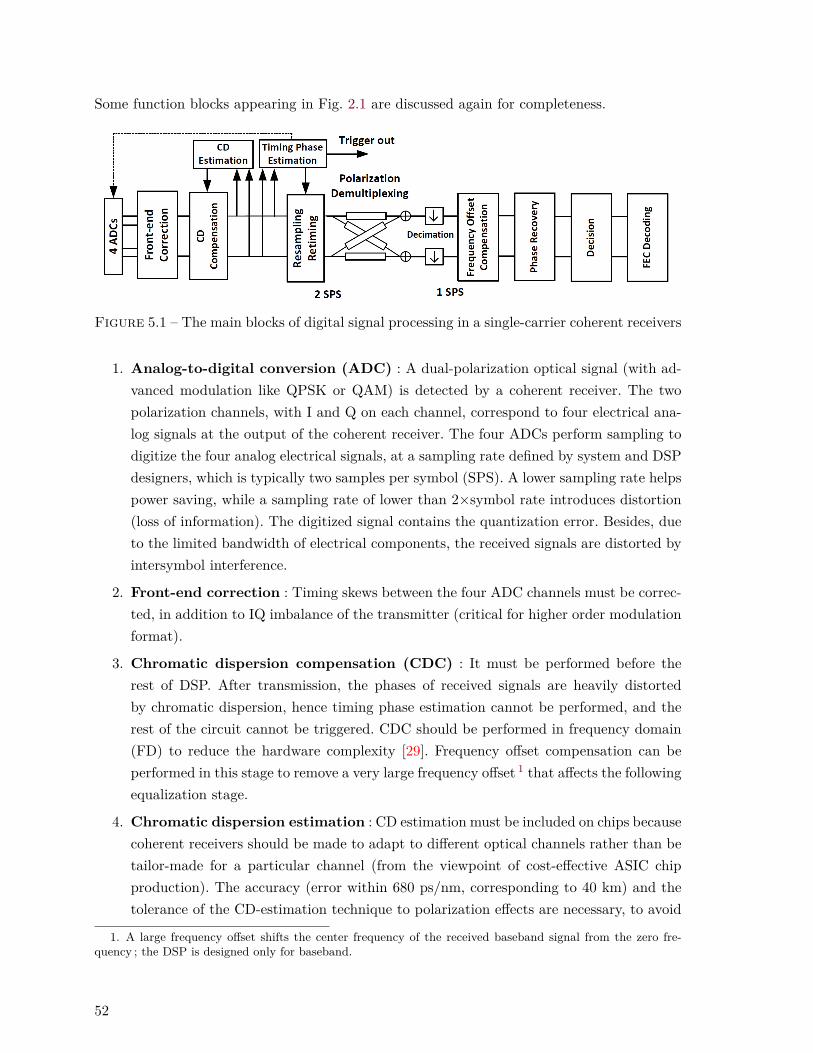
Some function blocks appearing in Fig. 2.1 are discussed again for completeness.

Figure 5.1 – The main blocks of digital signal processing in a single-carrier coherent receivers

1. Analog-to-digital conversion (ADC) : A dual-polarization optical signal (with ad-vanced modulation like QPSK or QAM) is detected by a coherent receiver. The twopolarization channels, with I and Q on each channel, correspond to four electrical ana-log signals at the output of the coherent receiver. The four ADCs perform sampling todigitize the four analog electrical signals, at a sampling rate defined by system and DSPdesigners, which is typically two samples per symbol (SPS). A lower sampling rate helpspower saving, while a sampling rate of lower than 2×symbol rate introduces distortion(loss of information). The digitized signal contains the quantization error. Besides, dueto the limited bandwidth of electrical components, the received signals are distorted byintersymbol interference.

2. Front-end correction : Timing skews between the four ADC channels must be correc-ted, in addition to IQ imbalance of the transmitter (critical for higher order modulationformat).

3. Chromatic dispersion compensation (CDC) : It must be performed before therest of DSP. After transmission, the phases of received signals are heavily distortedby chromatic dispersion, hence timing phase estimation cannot be performed, and therest of the circuit cannot be triggered. CDC should be performed in frequency domain(FD) to reduce the hardware complexity [29]. Frequency offset compensation can beperformed in this stage to remove a very large frequency offset 1 that affects the followingequalization stage.

4. Chromatic dispersion estimation : CD estimation must be included on chips becausecoherent receivers should be made to adapt to different optical channels rather than betailor-made for a particular channel (from the viewpoint of cost-effective ASIC chipproduction). The accuracy (error within 680 ps/nm, corresponding to 40 km) and thetolerance of the CD-estimation technique to polarization effects are necessary, to avoid

1. A large frequency offset shifts the center frequency of the received baseband signal from the zero fre-quency ; the DSP is designed only for baseband.

52

large OSNR penalty and unstable performance (large outage probability discussed inChapter 6). One of the common techniques is based on the clock tone magnitude [57].

5. Timing phase estimation (TPE) : After CDC, the received signals become morecoherent 2, allowing us to extract the timing phase. ADC Sampling instants will be ske-wed in the presence of clock frequency or timing phase mismatch between transmittersand receivers. Timing phase estimation is necessary during resampling and retiming tocorrect the sampling instant. The estimate can also be fed back to the ADCs for adjus-ting the sampling instant. However, the polarization effects and the bulk CD weakenthe clock tone magnitude and distort the true timing phase. For the details of timingphase estimation, please refer to Appendix G.

6. Resampling and retiming : The clock frequency (of electronics) between transmit-ters and receivers may not be the same. It is likely that the sampling rate is less than2×symbol rate in order to reduce the overall power consumption (For example, in Chap-ter 6, a 32 Gbaud signal is sampled at 40 Gsamples/s). Interpolation is performed toupsample to 2-SPS for the subsequent polarization demultiplexing. The retiming is per-formed by using the sampling phase estimated by TPE.

7. Polarization demultiplexing : In time-domain polarization demultiplexing, one usesthe MIMO approach with T/2-spaced finite-impulse-response filters, which requires a2-SPS input signal. It is mainly to compensate the polarization effects of an opticalchannel. The functions of MIMO will be discussed in Section 5.4 in detail.

8. Decimation from 2-SPS to 1-SPS is necessary after polarization demultiplexing.This helps reduce power consumption. The frequency offset compensation is performedto compensate the frequency mismatch between the transmit and receive lasers (whichrotates the signal constellation).

9. Phase recovery : The laser phase noise rotates the constellation randomly. Phase noiseestimation algorithms are required. Please refer to Chapter 2.

10. Hard decision : Only hard decision is considered in this thesis for symbol detection.

11. FEC decoding : Channel coding is beyond the scope of this thesis. The bit-error ratesmentioned in this thesis are all without channel coding.

5.2 Model of fiber polarization effects

After the introduction of the main DSP blocks in a dual-polarization digital coherent receiver,this section will give a simple model that represents polarization effects in an optical channel.As chromatic dispersion (CD) is a relatively time-invariant effect compared to polarization

2. The CD-distorted coherent signals are not coherent as if they are random noises, since their phases areheavily distorted by the fiber dispersion. After CDC, the signals become "coherent" again, meaning a higherinformation content can be obtained from the data.

53

effects, we compensate the bulk CD before MIMO processing as mentioned in the previoussection. The polarization effect of the fiber channel can therefore be modeled, in the frequencydomain, as :

H(f) =[cos θ sin θ−sin θ cos θ

] [ej(2πfτ+φ)/2 0

0 e−j(2πfτ+φ)/2

] [cos θ −sin θsin θ cos θ

](5.1)

where θ is the polarization orientation angle, φ is the phase delay between the optical fieldson X and Y polarizations, τ is the differential group delay (DGD) due to polarization modedispersion (PMD) in single-mode fiber (SMF).

For polarization demultiplexing, one has to compensate the effect of the optical channel in(5.1). As Jones matrix (5.1) acts on the field, one has to known both amplitude and phaseof the received signal. This is the reason we require coherent detection system to double thespectral efficiency by using dual-polarization transmitted signals.

5.3 Conventional MIMO

In this section, the conventional MIMO for polarization demultiplexing will be revisited withinput from [25, 26, 27, 36]

After CD compensation, resampling is performed to give 2 SPS. Retiming can be skippedbefore MIMO because the FIR filters of MIMO provide retiming via its interpolation property.Let Xin and Y in be the input signals of the MIMO corresponding to X and Y polarizationchannels, with two SPS.Xin and Y in suffer from the polarization crosstalks due to polarizationrotation and DGD from each other, represented by the Jones matrix in (5.1). Our goal is toequalize this Jones matrix.

Let Xkin be a 2-SPS input sequence that is convolved with two FIR filters hkxx and hkyx, where

k is the time index (increase by one for every sampling duration). All vectors here have thelength of N , where N is the FIR filter length (number of taps). Similarly, Y k

in is an 2-SPSinput sequence that is convolved with two FIR filters hkyy and hkxy. The outputs of MIMO,Xout(k) and Yout(k), for X- and Y-polarizations respectively, are :

Xout = hkxx ·Xkin + hkxy · Y in (5.2)

Yout = hkyx ·Xkin + hkyy · Y in (5.3)

54

where

Xkin = [Xin,k, Xin,k−1, . . . , Xin,k−N+1]T (5.4)

Y kin = [Yin,k, Yin,k−1, . . . , Yin,k−N+1]T (5.5)

hkxx = [hkxx,0, hkxx,1, . . . , hkxx,0]T (5.6)

hkxy = [hkxy,0, hkxy,1, . . . , hkxy,0]T (5.7)

hkyx = [hkyx,0, hkyx,1, . . . , hkyx,0]T (5.8)

hkyy = [hkyy,0, hkyy,1, . . . , hkyy,0]T (5.9)

The above FIR filters are adaptively updated by error signals, via a set of stochastic gradientalgorithm equations with step-size parameter µ :

hk+1ij = hkij + µ

∂

∂hkij∇J (5.10)

where i and j can be x or y, ∇J is the averaged error signal depending on the criterion usedfor equalization. Typically, a blind adaptive approach is used based on constant modulusalgorithm (CMA), such that the averaged error signal, ∇JCMA, is

∇JCMA = E[(|Akout|2 −R)2

](5.11)

where E denotes the expectation taken over the received samples, R is the average powerof the QAM signal, Ak is either an output vector on either X or Y, depending on whichpolarization channel is chosen to be the output of FIR filters.

In practice, instantaneous error signals are used instead of an averaged error signal becausethe averaging requires long memory depth, i.e., ∇JkCMA = (|Akout|2−R)2. The set of equationsof the gradient algorithm becomes :

hk+1xx = hkxx + µex(k′)Xout(k)Xk

in (5.12)

hk+1xy = hkxy + µex(k′)Xout(k)Y k

in (5.13)

hk+1yx = hkyx + µey(k′)Yout(k)Xk

in (5.14)

hk+1yy = hkyy + µey(k′)Yout(k)Y k

in (5.15)

where

ex(k′) = |Xout(k′)|2 −R (5.16)

ey(k′) = |Yout(k′)|2 −R (5.17)

are the instantaneous error signals for X- and Y-polarization channels, respectively. Note thatthe set of equations (5.12) is updated only at every two samples, such that k′ = k−mod(k, 2) 3,

3. mod(k, 2) is defined as the remainder after division of k by 2.

55

while the FIR filters hkij is convolved with the input sequence samplewise. In this way, theFIR filters provide the retiming ability by shifting and interpolating samples.

As the instantaneous error has to be calculated to update the tap coefficients, feedback loopsexist in real-time system. However, as the polarization effects ([5]) are slow compared to sym-bol rate, MIMO performance degradation is negligible compared to real-time phase tracking,as mentioned in Chapter 3.

Numerous works [77, 76, 9] demonstrate that following convergence of CMA, switching theerror function in (5.11) from CMA to decision-directed least-mean square (DD-LMS) canfurther help improve the BER performance. However, DD-LMS requires symbol decisions afterthe phase recovery, resulting in a much larger feedback delay (between MIMO, frequency offsetcompensation, phase recovery) for implementation. Symbol decisions are performed duringor after phase recovery, meaning that the equalization of MIMO is phase sensitive (beingaffected by the symbol-wise phase noise). In this thesis, we do not consider DD-LMS as ourerror function in MIMO-FIRs.

5.4 Role of conventional MIMO

In the state-of-the-art 100 Gbps system, conventional MIMO compensates the polarizationeffects of optical channel. As polarization effects are slow compared to symbol rate or sam-pling rate, MIMO functions not only as an equalizer for polarization effect, but also otherequalization roles. The samplewise MIMO accomplishes the following functions :

1. Polarization derotation : The butterfly structure consists of four branches represen-ting the four entries of an inverse Jone matrix. The cross components, hkxy and hkyx areresponsible for compensating the crosstalk between two polarization channels.

2. ISI equalization : Equalization of the intersymbol interference (ISI) caused by limitedreceiver bandwidth is an intrinsic function of FIR filters.

3. Residual CD Equalization : Chromatic dispersion (CD) estimation is performedbefore the start of DSP shown in Fig. 5.1. However, the best CD estimation precisionfor long-haul transmission is only 40 km (corresponding to a residual CD of 680 ps/nm)[57]. The time-domain FIR filters must be long enough [50, 8] to compensate the residualCD to avoid large power penalty or a large system outage.

4. Retiming : Timing phase error due to the incorrect sampling instant introduced duringanalog-to-digital conversion [26] must be corrected before equalization. Timing phaseerror results in faulty equalization even with perfect knowledge of a channel. For aperfectly estimated inverse Jones matrix, analog-to-digital converters (ADCs) may notsample at the optimal points. The intrinsic time delay and interpolation properties ofFIR filters with T/2-spacing with at least 5 taps are essential to avoid the OSNR powerpenalty due to timing phase errors [26].

56

5. PMD compensation : The DGD introduces crosstalk between two polarizations. Thisimpairment can be adaptively compensated by the FIR filters of the cross componentsof the butterfly structure. For long-haul systems, the largest tap weights are usually afew taps off from the center, indicating a DGD of a few symbols introduced during thefiber transmission [9, 36].

5.5 Problems of conventional MIMO

Although MIMO provides several functions, it has the following problems :

1. Singularity problem : since the CMA is a blind algorithm, both X- and Y-polarizationchannels may converge to the same output [27, 72] ;

2. Long Convergence : Convergence time may be long for certain SOPs and for longerFIRs. The SOP-dependent convergence time, called the idle time, becomes critical foracquisition in burst-mode receivers for short-reach applications [35, 66, 33, 6] ;

3. Power Consumption : FIR filters are a sample-wise operation, which requires paral-lelization and a lot of multipliers to guarantee the equalization at sampling rate. It hashigh hardware complexity and is one of major power consumption, after CDC and FECin coherent receiver ASIC chips [58, 29] ;

4. Convergence Monitoring : Convergence monitoring is required in coherent receiversand increases ASIC chip areas.

5.6 Summary

In this chapter, an overview of the DSP architecture in dual-polarization single-carrier digitalcoherent receivers was given. MIMO is used to perform digital polarization demultiplexing,equivalent to multiplying the received sampled signal with a Jones matrix representing theinverse of the optical channel. We have mathematically formulated the MIMO FIR, in whichthe CMA is commonly chosen for FIR filter coefficient updates. Finally, the roles of MIMOwere explained : polarization derotation, ISI equalization, residual CD compensation, retimingand PMD compensation. The problems of MIMO, including the singularity problem, longconvergence, which leads to significant power consumption and chip area, will be solved byour proposed DSP in Chapter 6 and 7.

57

Chapitre 6

SOP Pre-rotation before MIMO

In Chapter 5, we have reviewed the background for digital polarization demultiplexing, andunderstood the functions and problems of MIMO. In the present chapter, we will proposea DSP technique to solve the problems of MIMO and reduce power consumption in short-reach coherent communications. First, we will give a background for our motivation. We willintroduce our proposed DSP architecture, its principle, and its implementation. We will gothrough the setup and results for our 100 Gb/s DPQPSK experiment with limited (16 GHz)receiver bandwidth. We will present a tradeoff between hardware reduction and performancedegradation in the presence of residual chromatic dispersion for short-reach applications.

6.1 Introduction

Power consumption is a concern

Commercial coherent receivers at 100 Gbit/s have been deployed for long-haul transmission.Short-reach applications at these rates can take advantage of coherent technology as com-ponent prices decline. For short reach, power consumption can be reduced in subsystems forchromatic dispersion compensation (CDC) and forward error correction (FEC) from 50 W to3 W [29, 58]. After CDC and FEC, polarization demultiplexers with 2×2 adaptive multi-inputmulti-output (MIMO) half-symbol-spaced finite-impulse response (FIR) filters remain a ma-jor source of power consumption, due to the large number of multipliers used for parallelizingthe filters [5, 29].

For short-reach applications, PMD is much smaller than that in long-haul transmissions,and the length of FIR filters can be reduced. On the other hand, in the absence of channelimpairment, the minimum FIR filters with T/2-spacing with at least 5 taps [26] are essentialto mitigate residual timing phase errors as discussed in Chapter 5 1. A larger residual CD

1. Although the FIR filters correct the timing phase error due to their intrinsic interpolation ability [26],in practice, timing phase estimation algorithms are applied before the MIMO-FIRs to avoid time-consuming

59

requires longer FIR filters.

Retiming fails due to polarization effects

Other than chip power consumption, another practical concern is how we can obtain a clocksignal from the received sampled signal in order to trigger the rest of the chip. After trans-mission, the signal’s phase is heavily distorted by the fiber chromatic dispersion (CD), andtherefore the clock information totally disappears. Thus, CD compensation must be performedbefore other equalizations. As shown in Fig. 5.1, CD estimation must be performed before CDcompensation. For short reach systems (less than 100 km) or for long-haul coherent systemswith optical or digital CD compensation, CD is not strong enough to totally suppress theclock information. Polarization effects, namely, polarization rotation and polarization modedispersion, become the major impairments leading to failure our timing phase estimation(TPE) [57, 19].

For certain states of polarization (SOPs), the clock tone of signals completely disappearsand TPE fails for half-symbol delay, or half-baud differential group delay (DGD)[19, 20, 31].Loss of clock can be circumvented by pre-rotating the SOP to avoid 45-degree SOPs [62],or by applying the maximization of clock tones produced by various test SOPs [59, 60].These feedback approaches, however, involve sophisticated DSP algorithms at symbol ratesor higher and substantial numbers of block-wise multipliers [20, 62, 59, 60, 71]. Thus, thesesolutions are power hungry and increase implementation complexity. They exploit SOP pre-rotation (PR) before MIMO only to obtain a better clock phase, not to assist polarizationdemultiplexing. In the subsequent DSP, MIMO repeat the task of polarization rotation forpolarization demultiplexing. For more information about TPE and clock tone, please refer toAppendix G.

Our contributions

In this chapter, we limit our attention to short-reach transmission (below 100 km), whereDGD is present but not prominent 2. We propose a novel parallelizable DSP architecture, toperform a very coarse SOP pre-rotation before MIMO using an inverse Jones matrix based onthe minimization of only a single Stokes parameter (s1). This SOP pre-rotation can coarselyreject the polarization crosstalk before the subsequent polarization demultiplexing DSP. Itoffers several advantages compared to the conventional MIMO-FIR approaches :

1. It requires only a single Stokes parameter (s1) instead of all three Stokes parametersused in metrological algorithms in Appendix H, greatly reducing the computational

MIMO convergence. The residual timing phase errors due to estimation inaccuracy are then corrected byMIMO-FIRs.

2. According to Chapter 1 in [1], the PMD parameter Dp is 0.1-1 ps/km 12 . The corresponding DGD is

calculated as Dp√L, where L is the fiber length. For 40 km SMF, the the DGD value should be below 0.1

×√

40 = 6.3 ps. However, Dp is 0.05 ps/km 12 in commerical fibers, i.e., the (mean) DGD value is 0.3 ps [37].

60

effort ;

2. It avoids the problem of long MIMO convergence and singularity for certain SOPs ;

3. Thanks to the reduced polarization coupling, we are then at liberty to reduce the numberof MIMO cross-taps, leading to a significant reduction in number of MIMO-FIR CMs.

4. The SOP pre-rotation also brings the benefit of restoring clock tones for TPE evenbefore MIMO. The overhead for coarse SOP estimation is easily counter balanced bysavings in MIMO complexity.

Figure 6.1 – DSP architecture with reduced cross-FIR taps. CDC : chromatic dispersioncompensation. ADC : analog-to-digital conversion. SS-SOP : Stokes space state of polarization.

6.2 Proposal DSP Architecture

6.2.1 Overall Architecture

Fig. 6.1 shows our proposed DSP architecture. CDC is performed on the 4-channel sampleddata. As SOP rotation (even in a long-haul system) is a slowly varying process compared tosymbol rate, SOP estimation is only required at application-specific integrated circuit (ASIC)clock rates, which are below 500 MHz [50]. We propose our SOP estimation and SOP pre-rotation as shown in the two orange blocks in Fig. 6.1 : A very coarse SOP search in Stokesspace (see Section 6.3) is performed continuously at every four ASIC clocks ; the numberof ASIC clock cycles depends on the speed of SOP variation in the channel. The incomingdata samples are pre-rotated at the sampling rate by an inverse Jones matrix using 12 realmultiplies (RMs), a matrix calculated from the estimated SOP using Stokes parameter s1.Finally, the interpolator resamples to two samples per symbol for the subsequent 2×2 MIMOT/2-spaced FIR filters. All other signal processing proceeds on the demultiplexed signals.

We propose to implement the MIMO-FIRs with reduced cross filter lengths (later we callit the reduced-complexity MIMO), as smaller FIRs are sufficient to compensate the small

61

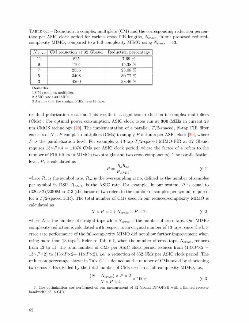
Table 6.1 – Reduction in complex multiplers (CM) and the corresponding reduction percen-tage per ASIC clock period for various cross FIR lengths, Ncross, in our proposed reduced-complexity MIMO, compared to a full-complexity MIMO using Ncross = 13.

Ncross CM reduction at 32 Gbaud Reduction percentage11 825 7.69 %9 1704 15.38 %7 2556 23.08 %5 3408 30.77 %3 4260 38.46 %

Remarks :1 CM : complex multiplier.2 ASIC rate : 300 MHz.3 Assume that the straight FIRS have 13 taps.

residual polarization rotation. This results in a significant reduction in complex multipliers(CMs) : For optimal power consumption, ASIC clock rates run at 300 MHz in current 28nm CMOS technology [29]. The implementation of a parallel, T/2-spaced, N -tap FIR filterconsists of N ×P complex multipliers (CMs) to supply P outputs per ASIC clock [29], whereP is the parallelization level. For example, a 13-tap T/2-spaced MIMO-FIR at 32 Gbaudrequires 13×P×4 = 11076 CMs per ASIC clock period, where the factor of 4 refers to thenumber of FIR filters in MIMO (two straight and two cross components). The parallelizationlevel, P , is calculated as

P = RsRosRASIC

, (6.1)

where Rs is the symbol rate, Ros is the oversampling ratio, defined as the number of samplesper symbol in DSP, RASIC is the ASIC rate. For example, in our system, P is equal to(32G×2)/300M ≈ 213 (the factor of two refers to the number of samples per symbol requiredfor a T/2-spaced FIR). The total number of CMs used in our reduced-complexity MIMO iscalculated as

N × P × 2 +Ncross × P × 2, (6.2)

where N is the number of straight taps while Ncross is the number of cross taps. Our MIMOcomplexity reduction is calculated with respect to an original number of 13 taps, since the bit-error rate performance of the full-complexity MIMO did not show further improvement whenusing more than 13 taps 3. Refer to Tab. 6.1, when the number of cross taps, Ncross, reducesfrom 13 to 11, the total number of CMs per ASIC clock period reduces from (13×P×2 +13×P×2) to (13×P×2+ 11×P×2), i.e., a reduction of 852 CMs per ASIC clock period. Thereduction percentage shown in Tab. 6.1 is defined as the number of CMs saved by shorteningtwo cross FIRs divided by the total number of CMs used in a full-complexity MIMO, i.e.,

(N −Ncross)× P × 2N × P × 4 × 100%. (6.3)

3. The optimization was performed on our measurement of 32 Gbaud DP-QPSK with a limited receiverbandwidth of 16 GHz.

62

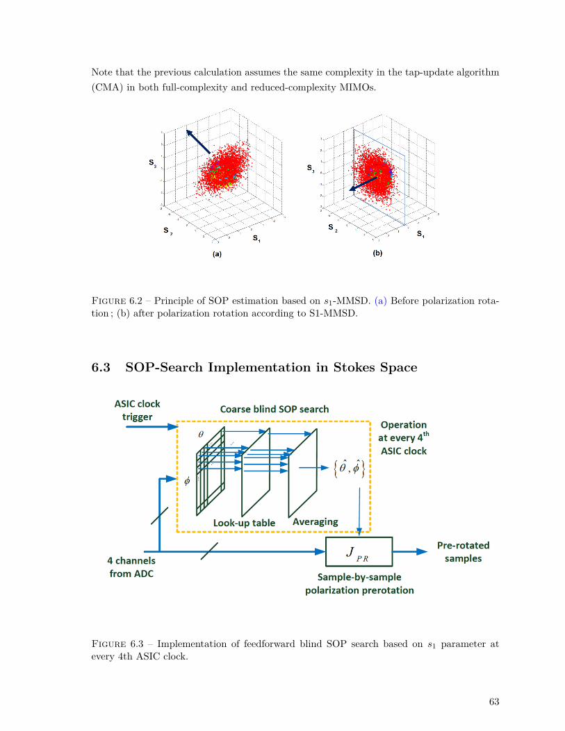
Note that the previous calculation assumes the same complexity in the tap-update algorithm(CMA) in both full-complexity and reduced-complexity MIMOs.

Figure 6.2 – Principle of SOP estimation based on s1-MMSD. (a) Before polarization rota-tion ; (b) after polarization rotation according to S1-MMSD.

6.3 SOP-Search Implementation in Stokes Space

Figure 6.3 – Implementation of feedforward blind SOP search based on s1 parameter atevery 4th ASIC clock.

63

Szafraniec et al. [63, 64] and Muga et al. [38] applied a plane fitting and a classical adaptivetracking algorithm, respectively, to obtain an inverse Jones matrix based on the Stokes pa-rameters of a normal to the lens-shaped object (Please refer to Appendix H or Section 3.2in [64]) . After SOP rotation, the resultant signals have similar power on X and Y polariza-tions. These methods evaluated all three Stokes parameters, leading to significant increasedcomplexity.

Instead of evaluating three Stokes parameters with plane fitting or tracking, we find the SOPestimate, s, (i.e., the polarization angle θ and the phase delay φ between two polarizations)via the minimum mean squared distance (MMSD) between the received samples and the planeat s1 = 0 as shown in Fig. 6.2, i.e.,

s = minsE[|s1|2], (6.4)

where s1 is the first Stokes parameter [63] defined as

s1∆= |Ex|2 − |Ey|2, (6.5)

with Ex and Ey representing the complex fields at the X- and Y-polarizations with respectto coherent receiver. As Stokes parameters are functions of Jones-space parameters, θ and φ,we will minimize |s1|2 in terms of θ and φ, instead of Stokes vector s. For convenience, fromnow on we will call "minimizing s1" insteand of |s1|2. This results in a 2-D SOP blind searchbased on minimizing s1, i.e., (6.4) is equivalent to the following :{

θ, φ}

= min{θ,φ}

E[|s1|2]. (6.6)

First, the received complex signals in both polarizations are rotated by various Jones matricesin parallel (12 RMs) [51], as shown in the first stage of the dotted box in Fig. 6.3 :

JPR =[cos θ − sin θeiφ

sin θ cos θeiφ

](6.7)

where the negative sign acts as a constraint to avoid the non-physical singularity that troublesthe constant modulus algorithm [27] 4. We use only 10◦ resolution for both θ (spanning 90◦)and φ (spanning 180◦), which requires 18×9×12 = 1944 RMs or 486 CMs each time.

4. The unitary representation of the Jones matrix acts as a natural constraint to prevent the non-physicalsingularity, where singularity refers to the outcome that two polarization channels at the output converge tothe same polarization channel data [27]. To see that our JPR is unitary, (7.14) can be written as

JPR =[

cos θ − sin θsin θ cos θ

][1 00 eiφ

]. (6.8)

The term eiφ represents the phase delay between x and y polarizations. Since Jones representation depends onthe relative polarization angle and phase between x and y polarizations, a common phase factor e−iφ/2 can beintroduced to x and y polarizations in (6.9) :

JPR =[

cos θ − sin θsin θ cos θ

][e−iφ/2 0

0 eiφ/2

]=[

cos θe−iφ/2 − sin θe−iφ/2sin θeiφ/2 cos θeiφ/2

]. (6.9)

The determinant of JPR is one.

64

As the SOP rotation is slow, we need only acquire samples and perform the SOP estimationat every four ASIC clocks, i.e., 121.5 CMs per clock. This increase in CMs is compensatedby the reduced number of CMs in our modified MIMO-FIRs shown in Tab. 6.1. The 18×9 =162 rotated complex fields will be converted to the corresponding s1 (and thus |s1|2) usinglook-up tables. The result is saved into registers and added to the next s1 values. An averageis taken over a block of 200 samples (time-interleaved at every four ASIC clock periods) togenerate the mean squared distance (MSD). The optimal SOP corresponding to MMSD ischosen by comparator circuitry. The two-dimensional MSD surface is shown in Fig. 6.4.

Figure 6.4 – The surface of the mean squared distance (MSD) of S1 parameter. Red dotrefers to the MMSD (the optimal SOP).

Finally, we rotate every sample using 12 RMs using the optimal SOP, requiring 3× (fs/300MHz) CMs per ASIC clock period, where fs is the sampling frequency, as shown in the lowerpart of Fig. 6.3. In our work, fs is 40 GHz, and the total number of the required CMs perclock period is 400 + 121.5 = 521.5. Tab. 6.1 shows that, for 32 Gbaud DP-QPSK, the overallCM reduction starts when reducing Ncross by more than two. Obviously, the computationcomplexity can be further reduced by using cascaded blind search.

6.4 Experimental Setup

The performance of our proposed DSP is examined using the experimental setup shown inFig. 6.5. A 32 Gbaud DPQPSK signal was generated by a polarization multiplexing emulator(dashed, orange), with laser sources of 10 kHz linewidth. An Agilent N7786B polarizationsynthesizer was used to change the SOP of the transmitted signal. After passing through anerbium doped fiber amplifier (EDFA) and 40 km standard single-mode fiber (SMF) fiber, the

65

Figure 6.5 – Experimental setup for 32 Gbaud DP-QPSK 40 km transmission. PC : Polariza-tion controller, IQ Mod. : Inphase-Quadrature modulator, Pol. Syn. : Polarization synthesis,OBPF : optical band pass filter, OTDL : Optical tunable delay line, OSA : optical spectrumanalyser, RTO : real-time oscilloscope, EDFA : erbium doped fiber amplifier, VOA : variableoptical attenuator, Coh. Rx. : Coherent receiver.

received signal was coherently detected by an integrated coherent receiver having a bandwidthof 22 GHz. The real-time oscilloscope (ADC) sampled at 40 GSa/s with bandwidth of 16 GHz.Offline processing was used and 1,120,000 bits were used for bit error rate (BER) measurement.

Table 6.2 – Cases considered for BER performance analysis.

Case SOP-PR Ncross CMs for PR CMs for MIMO Acq. time CDC before MIMOX No 13 None 11076 long lowA Yes 13 None 11076 short lowB Yes 7, 5 521.5 8520, 7668 short mediumC No 7, 5 521.5 8520, 7668 long medium

Remarks :1 SOP : state-of-polarization ;2 PR : pre-rotation ;3 CM : complex multipliers (per ASIC clock period) ;4 Acq. : acquisition ;5 CDC : chromatic dispersion compensation.

For DSP, the flow shown in Fig. 6.1 was used. CDC was first performed on the capturedsamples. Then a conventional MIMO approach and our proposed DSP for polarization de-multiplexing were performed. Tab. 6.2 shows four cases of interest in this chapter, assumingthe same parameters (i.e. 32 Gbaud, 13 straight taps, variable cross tap numbers) as Tab. 6.1.In all cases, the CMA algorithm was employed for calculating the errors and updating theFIR taps as explained in Chapter 5. After polarization demultiplexing, standard algorithmsfor frequency offset compensation and carrier phase recovery were performed, followed bydetection and bit error counting.

66

Case X refers to the conventional MIMO-FIR, where the acquisition time can be long for cer-tain SOPs. Case A refers to the conventional MIMO-FIR with our proposed SOP estimation/pre-rotation (PR), which reduces the acquisition time but otherwise leaves performance unchan-ged 5. Case B refers to our approach, in which we have our proposed SOP-estimation/SOP-PR and we reduce the MIMO-FIR cross taps from 13 to 7 and 5, respectively. Case C issimilar to Case B, but without SOP estimation/SOP-PR. Case C is a control to allow us tounderstand the importance of SOP-PR for reduced-complexity MIMO. As Case X and CaseA make use of more cross taps, they are expected to have a better CD tolerance and requiresless effort for CDC before MIMO compared to Case B and Case C. We do not repeat caseX, since Case A will share the same BER performance result, except that it requires a longeracquisition time.Tap initialization is important in both real-time and offline DSP. In the state-of-the-art di-gital coherent receivers, training sequences are employed to reduce the convergence time oftap values [45, 46], sacrificing transmission capacity. In offline DSP, convergence time of theCMA algorithm should be minimized, so that we can calculate BER faster. One may expectthat the reduced-complexity MIMO should converge faster than the full-complexity MIMObecause of shorter tap length. However, based on our finding, the "overly" reduced-complexityMIMO (i.e., Ncross = 5) cannot converge at all because of the large error signal (the tapupdates via CMA depends on the error signals).

In our offline DSP, the full-complexity MIMO (with Ncross = 13) in case A requires no tapinitialization. The tap values can finally converge, and the error signal stays small after conver-gence because the FIR taps are long enough for equalization. However, singularity may occur.In our measurement, SOP estimation/PR was performed to speed up the convergence (andavoid singularity) for saving our processing time. In contrast, the reduced-complexity MIMOin case B and case C should require tap initialization, since inadequate numbers of cross tapsresult in partial equalization, and thus larger error signals and fluctuation, leading to erro-neous tap-value calculations and failure of convergence. This tap initialization was replacedby our proposed SOP estimation/PR, which compensates coarsely the polarization effects, re-ducing the effort in tap convergence, as shown in the blue curves in Fig. 6.6. However, withoutSOP estimation/PR, tap initialization was performed by using the information from the bestcase (case A ; full-complexity MIMO) after all taps converge, as shown in the black curves inFig. 6.6. We employed the SOP pre-knowledge only for achieving the best performance forcase C (without SOP estimation/PR), i.e., the BER performance of case C shown in Fig. 6.6is already the best that the reduced-complexity MIMO can achieve.

67

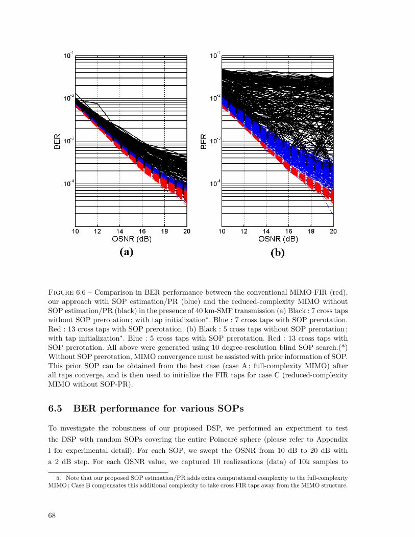
Figure 6.6 – Comparison in BER performance between the conventional MIMO-FIR (red),our approach with SOP estimation/PR (blue) and the reduced-complexity MIMO withoutSOP estimation/PR (black) in the presence of 40 km-SMF transmission (a) Black : 7 cross tapswithout SOP prerotation ; with tap initialization∗. Blue : 7 cross taps with SOP prerotation.Red : 13 cross taps with SOP prerotation. (b) Black : 5 cross taps without SOP prerotation ;with tap initialization∗. Blue : 5 cross taps with SOP prerotation. Red : 13 cross taps withSOP prerotation. All above were generated using 10 degree-resolution blind SOP search.(*)Without SOP prerotation, MIMO convergence must be assisted with prior information of SOP.This prior SOP can be obtained from the best case (case A ; full-complexity MIMO) afterall taps converge, and is then used to initialize the FIR taps for case C (reduced-complexityMIMO without SOP-PR).

6.5 BER performance for various SOPs

To investigate the robustness of our proposed DSP, we performed an experiment to testthe DSP with random SOPs covering the entire Poincaré sphere (please refer to AppendixI for experimental detail). For each SOP, we swept the OSNR from 10 dB to 20 dB witha 2 dB step. For each OSNR value, we captured 10 realizsations (data) of 10k samples to

5. Note that our proposed SOP estimation/PR adds extra computational complexity to the full-complexityMIMO ; Case B compensates this additional complexity to take cross FIR taps away from the MIMO structure.

68

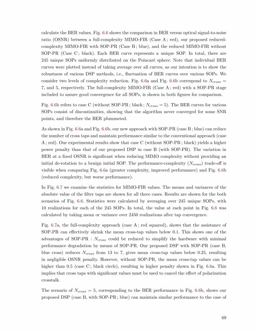
calculate the BER values. Fig. 6.6 shows the comparison in BER versus optical signal-to-noiseratio (OSNR) between a full-complexity MIMO-FIR (Case A ; red), our proposed reduced-complexity MIMO-FIR with SOP-PR (Case B ; blue), and the reduced MIMO-FIR withoutSOP-PR (Case C ; black). Each BER curve represents a unique SOP. In total, there are245 unique SOPs uniformly distributed on the Poincaré sphere. Note that individual BERcurves were plotted instead of taking average over all curves, as our intention is to show therobustness of various DSP methods, i.e., fluctuation of BER curves over various SOPs. Weconsider two levels of complexity reduction. Fig. 6.6a and Fig. 6.6b correspond to Ncross =7, and 5, respectively. The full-complexity MIMO-FIR (Case A ; red) with a SOP-PR stageincluded to assure good convergence for all SOPs, is shown in both figures for comparison.

Fig. 6.6b refers to case C (without SOP-PR ; black ; Ncross = 5). The BER curves for variousSOPs consist of discontinuities, showing that the algorithm never converged for some SNRpoints, and therefore the BER plummeted.

As shown in Fig. 6.6a and Fig. 6.6b, our new approach with SOP-PR (case B ; blue) can reducethe number of cross taps and maintain performance similar to the conventional approach (caseA ; red). Our experimental results show that case C (without SOP-PR ; black) yields a higherpower penalty than that of our proposed DSP in case B (with SOP-PR). The variation inBER at a fixed OSNR is significant when reducing MIMO complexity without providing aninitial de-rotation to a benign initial SOP. The performance-complexity (Ncross) trade-off isvisible when comparing Fig. 6.6a (greater complexity, improved performance) and Fig. 6.6b(reduced complexity, but worse performance).

In Fig. 6.7 we examine the statistics for MIMO-FIR values. The means and variances of theabsolute value of the filter taps are shown for all three cases. Results are shown for the bothscenarios of Fig. 6.6. Statistics were calculated by averaging over 245 unique SOPs, with10 realizations for each of the 245 SOPs. In total, the value at each point in Fig. 6.6 wascalculated by taking mean or variance over 2450 realizations after tap convergence.

Fig. 6.7a, the full-complexity approach (case A ; red squared), shows that the assistance ofSOP-PR can effectively shrink the mean cross-tap values below 0.1. This shows one of theadvantages of SOP-PR : Ncross could be reduced to simplify the hardware with minimalperformance degradation by means of SOP-PR. Our proposed DSP with SOP-PR (case B,blue cross) reduces Ncross from 13 to 7, gives mean cross-tap values below 0.25, resultingin negligible OSNR penalty. However, without SOP-PR, the mean cross-tap values can behigher than 0.5 (case C ; black circle), resulting in higher penalty shown in Fig. 6.6a. Thisimplies that cross taps with significant values must be used to cancel the effect of polarizationcrosstalk.

The scenario of Ncross = 5, corresponding to the BER performance in Fig. 6.6b, shows ourproposed DSP (case B, with SOP-PR ; blue) can maintain similar performance to the case of

69

Ncross = 7, allowing further reduction in CMs. Case C (without SOP-PR ; black) does notwork. Refer to Fig. 6.6b, one may argue that the vigorous BER fluctuation could be due tothe problems of our DSP algorithms. A better BER calculation should be obtained by payingmore effort on monitoring MIMO convergence in our DSP.

The BER fluctuation (discontinuities) and high OSNR penalty of case C could be a conse-quence of inadequate number of cross taps ; it is not caused by the problem in monitoringconvergence. The same CMA algorithm was applied to all cases, and we had already initializethe FIR taps in Case C by using the polarization information from case A (full-complexityMIMO). Fig. 6.6b shows that case C, without SOP-PR but with large tap reductions, does notwork at all with conventional standard DSP. We aim at showing the importance or necessityof using SOP estimation/PR for the reduced-complexity MIMO.

In Fig. 6.7b, the mean cross-tap values of our proposed DSP (case B ; blue squared) are allbelow 0.3, hence the negligible OSNR penalty. However, case C (without SOP-PR) has meancross-tap values higher than 0.9. This is because CMA requires only the error signal from theFIR filters for calculating the tap values. Inadequate numbers of cross taps result in partialequalization and thus larger error signals and fluctuation, leading to erroneous tap-valuecalculations even in the presence of SOP pre-knowledge.

We next examine the required precision for our blind SOP search. Could further precision inSOP estimation lead to even greater savings in MIMO-FIR complexity ? Fig. 6.8 shows thecomparison between 10 degree and 1 degree SOP search resolution for the case of Ncross = 5after 40-km full CDC. Surprisingly, 10 degree resolution is already sufficient for maintainingBER performance similar to that of 1-degree resolution. We have not tried a detailed opti-mization in terms of resolution and penalty, as we only address the novelty of our proposedDSP. Note that a very high SOP estimation is not necessary, as a pure SOP-PR using aninverse Jones matrix as in Stokes-space PolDemux (refer to our discussion in Appendix H),no matter how precise the resolution can be, is insufficient for achieving our performance.As discussed previously, the presence of cross-taps is indispensable for compensating resi-dual polarization-crosstalk and small DGD compensation and for retiming through the FIRinterpolation ability.

6.5.1 CD tolerance

CDC is an important source of power consumption in an ASIC chip [58, 29]. The ability of theMIMO-FIR to compensate residual CD should not be compromised, so that we can maintainCDC power consumption at the lowest possible level. In short-reach scenarios, CD exists andmust be compensated, but a separate DSP stage for CD compensation is not preferred. Thereason is pragmatic and cost-effective : OSNR is much higher than the OSNR threshold forFEC within 100 km transmission, and therefore system providers need only control the power

70

penalty due to residual CD within the link budget. In this section, we extend our analysisto examine tolerance to residual CD of our proposed DSP. Fig. 6.9a and Fig. 6.9b show theprobability mass functions (pmfs) of BER conditioned on different OSNRs values of cases A,B and C, which allow us to analyze the outage probability (Please refer to Section 6.7) in thepresence of residual CD for the case of Ncross = 7 and the case of Ncross = 5, respectively.We used the experimental set-up of 40 km transmission in Fig. 6.5. The CDC (shown inFig. 6.9) was set to compensate only 0, 20 and 40 km (680, 340 and 0 ps/nm residual CD,respectively) shown in green, red and blue, respectively. Although CD should be constant inour 40 km SMF, it becomes stochastic when the polarization crosstalk (which depends on theSOP distribution) can be not compensated perfectly by a reduced-complexity MIMO.

Generally, the mean of the pmf of BER shifts to higher values and the variance of the pmfof BER becomes larger when the residual CD increases. For example, considering Ncross =7 in Fig. 6.9a, our proposed DSP allows a 20 km short reach transmission (without CDC)at OSNR = 18 dB 6 with low system outage (a large portion of the pmf of BER is belowlog(BER) = -3, the FEC level). This tells us how Ncross should be to trim our coherent DSPcomplexity for a certain performance in short reach applications.

6.5.2 Restoration of Clock Tone Magnitude

In practice, after CDC, we resample the signal to 2 samples per symbol, which requires us todetermine the sampling phase using frequency-domain (FD) Godard timing phase estimation(TPE) [20, 62, 59, 60, 60, 71]. The principle of FD-Godard TPE is to obtain the phase ofthe autocorrelation function of the received signal (2 samples per symbol) spectrum at theclock frequency. The complex value of this autocorrelation function at the clock frequency isdefined as our complex-valued clock tone [57]. For more details, please refer to Appendix G.

The clock tone magnitude should be large enough to provide a good S-curve phase detectorfor timing phase recovery circuit [20, 62, 59, 60, 71]. It is shown in [22] that FD-Godard TPEis equivalent to the time-domain square-law nonlinearity TPE [41] which requires 4 samplesper symbol. One prefers to perform TPE and resampling in the frequency domain to minimizethe hardware complexity [57].

The previous TPE algorithms [59, 60, 61, 62] require SOP-PR to avoid clock tone loss dueto polarization effects. The advantage of using our proposed DSP is shown in Fig. 6.10, inwhich the clock tone magnitudes were obtained using FD-Godard TPE [57] over 780 variousunrepeated SOPs distributed over the Poincaré sphere. The conventional approach withoutSOP-PR (red) suffers from clock tone loss for certain SOPs (under small DGDs, polarizationdependent loss, timing offset between X and Y optical signals, and different sampling offsetsbetween X and Y analog-to-digital converters), leading to system failure of coherent receivers.

6. 18 dB or above are attainable OSNR values for shor t-reach systems.

71

Our proposed DSP with SOP-PR (black) can restore the weakened clock tone magnitude. Notethat in our experiment, the DGD introduced by the 40-km fiber span should be negligible. Weintroduced a fixed timing offset between X and Y at the transmitter using an optical tunabledelay line (OTDL) in Fig. 6.5 to emulate the loss of CT shown in Fig. 6.10 (red).

6.6 Conclusions

In this chapter, we demonstrated that an SOP pre-rotation (by multiplying the receivedsamples with an estimated Jones matrix corresponding to the inverse of an optical channel)can be performed before a conventional 2×2 MIMO for polarization demultiplexing. Its ad-vantages are to avoid long convergence of the conventional MIMO and singularity problems atcertain SOPs, suitable for applications requiring fast acquisition such as burst-mode receiversin packet-switching-based short-reach or metro network. The inverse Jones matrix requiresus to estimate the SOP, i.e., we generate our own channel-state information (CSI) beforepolarization demultiplexing is performed.

Firstly, instead of estimating SOPs using all three Stokes parameters (s1, s2, s3) with com-plicated plane fitting previously proposed for metrological purpose, we have proposed a verycoarse SOP estimation based on minimizing a single Stokes parameter, s1, to reduce the com-putational effort, with a 10-degree resolution only. Secondly, as this SOP pre-rotation cancoarsely reject the polarization crosstalk before the subsequent polarization demultiplexing,i.e. the polarization coupling is reduced, we are then at liberty to reduce the number of MIMOcross-taps, leading to a significant reduction in number of MIMO-FIR complex multiplica-tions, i.e., the overhead for coarse SOP estimation is easily counter balanced by savings inMIMO complexity. Finally, the SOP pre-rotation also brings the benefit of restoring clocktones for TPE even before PolDemux.

Our proposed DSP was validated by our experimental results in a 100 Gb/s DPQPSK systemwith limited (16 GHz) receiver bandwidth. We have also investigated a tradeoff between hard-ware reduction and performance degradation in the presence of residual chromatic dispersionfor short-reach applications.

6.7 Outpage Probability

The definition of outage probability in this work is given here. The values of BER of a 2×2MIMO-FIRs (CMA-based) with N straight taps and Ncross taps follows a probability densityfunction (pdf) conditioned on a given SOP (state-of-polarization) s, i.e. pN,Ncross(γ|s), wherethe SOP is described by azimuth angle θ (polarization rotation) and ellipticity angle φ (phasedelay between two polarizations). The outage probability of a 2×2 MIMO-FIRs (CMA-based)with N straight taps and Ncross taps is defined as the probability of which at a given OSNR,

72

the averaged BER is above a certain BER value γ, for example, FEC, i.e.

OPN,Ncross(FEC,OSNR) =∫γ>FEC

∫spN,Ncross(γ|s)fs(s)dsdγ (6.10)

where the pdf of SOPs fs(s) is assumed to be uniformly distributed over the Poincaresphere.Due to the limited number of realizations taken from our measurement, the corres-ponding probably mass functions (pmfs), PN,Ncross [γj |si] and Ps[si] are used instead of acontinuous pdf :

OPN,Ncross(FEC,OSNR) ≈∑

γj>FEC

∑si

PN,Ncross [γj |si]Ps[si] (6.11)

73

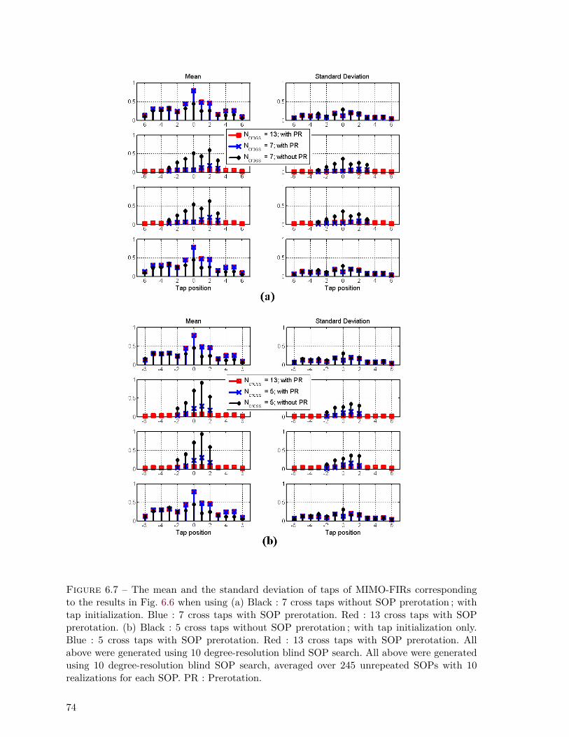
Figure 6.7 – The mean and the standard deviation of taps of MIMO-FIRs correspondingto the results in Fig. 6.6 when using (a) Black : 7 cross taps without SOP prerotation ; withtap initialization. Blue : 7 cross taps with SOP prerotation. Red : 13 cross taps with SOPprerotation. (b) Black : 5 cross taps without SOP prerotation ; with tap initialization only.Blue : 5 cross taps with SOP prerotation. Red : 13 cross taps with SOP prerotation. Allabove were generated using 10 degree-resolution blind SOP search. All above were generatedusing 10 degree-resolution blind SOP search, averaged over 245 unrepeated SOPs with 10realizations for each SOP. PR : Prerotation.

74

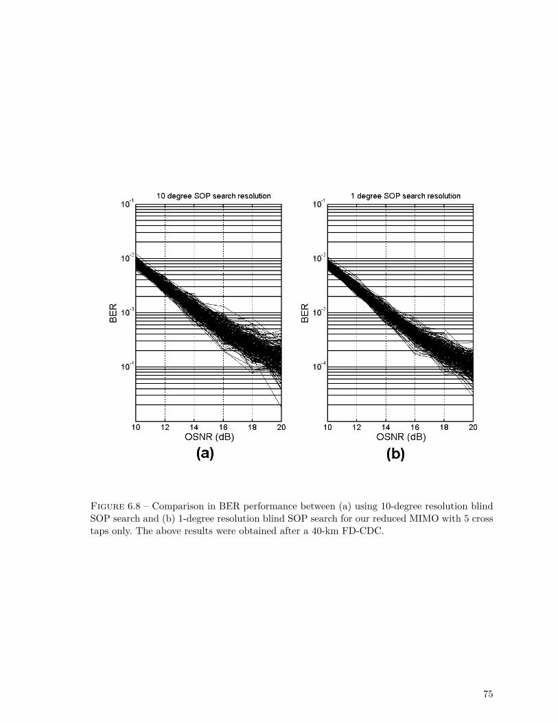
Figure 6.8 – Comparison in BER performance between (a) using 10-degree resolution blindSOP search and (b) 1-degree resolution blind SOP search for our reduced MIMO with 5 crosstaps only. The above results were obtained after a 40-km FD-CDC.

75

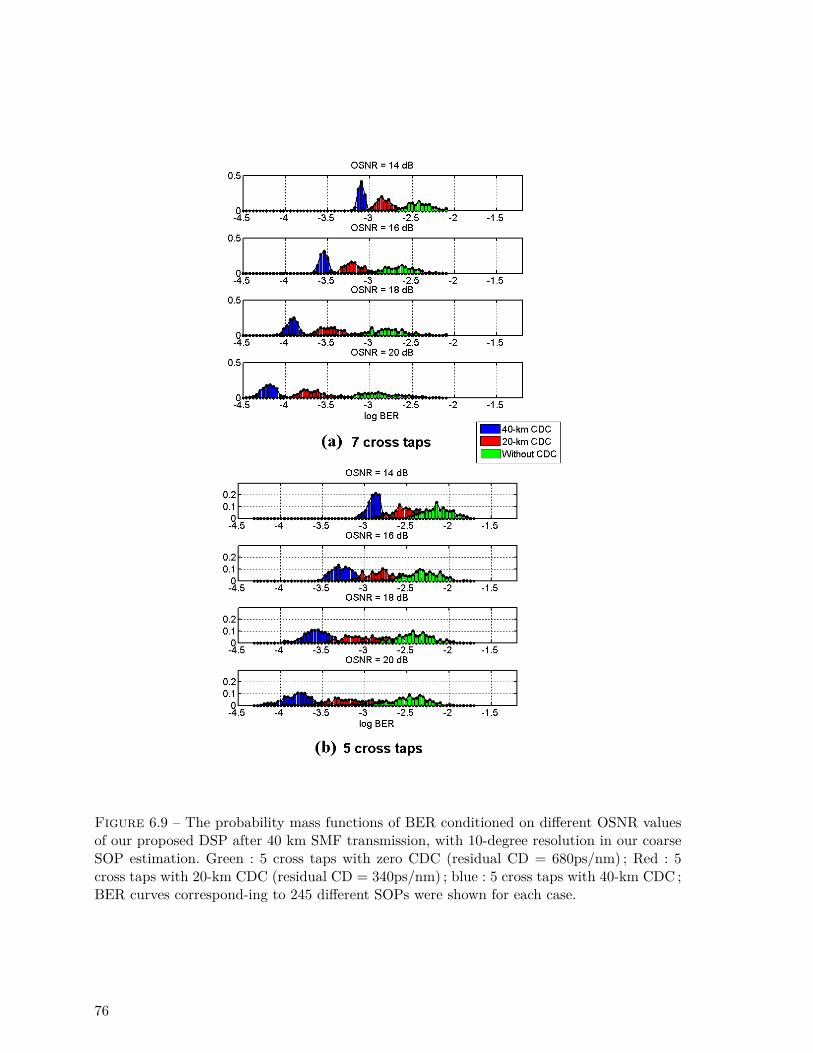
Figure 6.9 – The probability mass functions of BER conditioned on different OSNR valuesof our proposed DSP after 40 km SMF transmission, with 10-degree resolution in our coarseSOP estimation. Green : 5 cross taps with zero CDC (residual CD = 680ps/nm) ; Red : 5cross taps with 20-km CDC (residual CD = 340ps/nm) ; blue : 5 cross taps with 40-km CDC ;BER curves correspond-ing to 245 different SOPs were shown for each case.

76

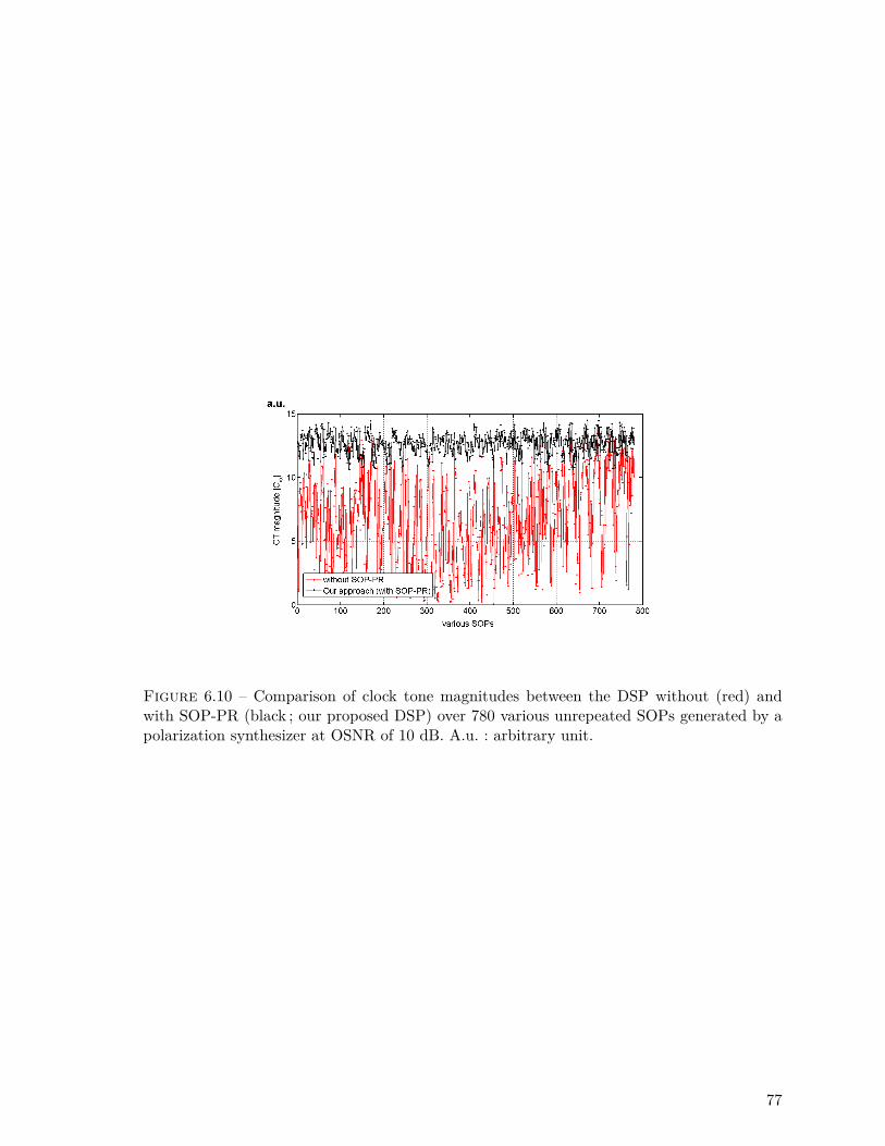
Figure 6.10 – Comparison of clock tone magnitudes between the DSP without (red) andwith SOP-PR (black ; our proposed DSP) over 780 various unrepeated SOPs generated by apolarization synthesizer at OSNR of 10 dB. A.u. : arbitrary unit.

77

Chapitre 7

Extended Kalman Filter-based SOPPre-rotation

In Chapter 6 we proposed a blind SOP search (parameterized by polarization orientation angleand phase delay between X and Y polarizations) to estimate the SOP of the received signal.The SOP was used for polarization pre-rotation to accelerate convergence and to reduce thehardware complexity of the conventional MIMO. Nevertheless, the blind SOP search requiresmemory to store the intermediate results calculated for each combination of parameters. Thischapter is an extension of Chapter 6. Here, we propose a SOP tracking using an extendedKalman filter to reduce the hardware complexity introduced by the blind SOP search inChapter 6.

The present chapter shares the same background and motivation with Chapter 6, which wasgiven in Section 6.1. We will first specify our contributions. We will review the formulationof a conventional discrete-time extended Kalman filter. Then we will discuss the formulationof our proposed low-complexity Kalman filter based on minimization of s1, as well as itsimplementation form. Finally, we will go through the experimental setup and our results fora polarization-scrambled (at 50 kHz) 32 Gbaud DP-QPSK system.

7.1 Contributions

SOP prerotation was first introduced for pure Stoke-space demultiplexing, primarily for ap-plications in metrology [63], despite its high computational complexity in estimating Stokesspace parameters for the input SOP. Appendix H provides a literature review for pure Stoke-space demultiplexing. Real-time implementation precludes high computation complexity andin Chapter 6, we thus proposed the use of a very coarse (with 10-degree resolution) blindsearch technique for SOP estimation. Nevertheless, blind search techniques are still conside-red computationally costly because the SOP estimation requires the averaging of resultants

79

from all SOP candidates, as shown in Fig. 6.3.

Kalman filter is well-known for its one-step operation, i.e., only the estimate(s) from theprevious iteration is required to estimate or predict the parameters in the following iteration.In the present chapter, we propose to use a low-complexity discrete-time extended Kalmanfilter (EKF) minimizing resultant s1 in order to track the inverse Jones matrix of an opticalchannel, reducing the memory depth required in our proposed blind SOP search in Chapter6. Our proposed algorithm is updated only at every ASIC clock period and can be applied toreal-time data.

The SOP prerotation allows us to obtain the clock information before MIMO, reducing thefeedback delay to the ADCs. We show that this EKF allows us to keep maintaining a goodclock tone magnitude level (which is important for timing phase estimation), has significantcomplexity reduction compared to the sample-wise multiplier blocks in timing-phase estima-tion algorithms [60, 62], and preserves all the advantages mentioned in Chapter 6, such asavoiding the singularity problem and long convergence of conventional MIMO, and reducingthe subsequent MIMO-filter taps.

7.2 Equations of Extended Kalman Filter

In this section, equations for the extended Kalman filter will be revisited. We will adhere tothe formulations from Szafraniec et al. [63], which uses the following notations :

– xk denotes the true parameter (also called the state vector).

– xk is the posteriori estimate of xk, which is an estimated state vector after the adjust-ment using the knowledge of measurement (as a posterior information). It is generatedin the measurement update equation. We use this vector for our estimated para-meters.

– x−k is the priori estimate of xk, which is an estimated state vector after the adjustmentusing the knowledge of parameter dynamics (as a prior information). It is generatedin the time update equation. In our proposed DSP, xk is the same as x−k as shownbelow.

7.2.1 Stochastic System

In the following, we start the standard formulation with scalar quantities for simplicity. Theformulation holds also for vector quantities.

We assume that our true time-varying parameter xk is described by a linear time differenceequation as follow :

xk = Axk−1 +Buk−1 + ζk−1, (7.1)

80

where the current state xk evolves from the previous state xk−1 through matrix A, uk repre-sents a perturbation that alters the parameters through matrix B, and ζk−1 represents thenoise in the system. Equation (7.1) is called the process equation, and ζk−1 is called theprocess noise.

Usually, one may not be able to observe the time-varying parameter directly upon measure-ment, i.e., xk is hidden in the measurement system h. We can only access the measurementoutput :

zk = h(xk) + ξk (7.2)

where ξk is the measurement noise. Function h can be either a linear or a nonlinear function.In this chapter, we only consider a nonlinear function for h. Equation (7.2) is called themeasurement equation. The following assumptions are used :

1. ζk is an uncorrelated sequence of zero mean random vectors with process-noise cova-riance variance Q.

2. ξk is an uncorrelated sequence of zero mean random vectors with measurement-noisecovariance variance R.

3. The initial state x0 has mean m0 and covariance Po

4. ζk, ξk and x0 are mutually uncorrelated.

The knowledge of matrices A, B and h (prior information) is crucial for us to apply theextended Kalman filter for tracking parameters.

7.2.2 Extended Kalman Filter Algorithm

Based on the above stochastic system, one can apply the standard extended Kalman filterstep-by-step. In the following, we will only revisit the procedures of EKF. For the EKFderivation, please refer to the standard textbook [47].

The EKF algorithm estimates the state vector (the desired parameters) using the time updateequations and the measurement update equations. The time update equations for statevector and for error covariance are :

x−k = Axk−1 +Buk−1, (7.3)

P−k = APk−1A∗T +Q, (7.4)

respectively, where Pk−1 is the covariance matrix of estimation error, P−k is the covariancematrix of estimation error after the adjustment using the knowledge of parameter dynamicsA and process noise Q. The measurement update equations are :

Kk = P−k H∗T (HP−k H

∗T +R)−1, (7.5)

81

xk = x−k +Kk(zk − h(x−k )), (7.6)

Pk = P−k −KkHP−k . (7.7)

where H is the Jacobian matrix of partial derivatives of function h with respect to state va-riables of xk. Kk in (7.5) refers to Kalman gain. The term, zk−h(x−k ), is called the innovation,or the instantaneous estimation error. The sequence of EKF is as follows :

1. Initialization at k = 1 : Substitute x0 into (7.3) and P0 and Q into (7.4).

2. Kalman gain update : Calculate the Kalman gain in in (7.5) using the result in (7.4)and R.

3. (a) Update estimate xk : Substitute x−k of (7.3), the new measurement output zk,Kalman gain Kk calculated in step 2 into (7.6).(b) Update State vector : In parallel to (a), Substitute P−k of (7.4) and Kalman gainKk calculated step 2 into (7.7).

4. Repeat the above for the next time index k.

7.3 EKF-based SOP Pre-rotation

Fig. 7.1a shows our proposed DSP flow, SOP pre-rotation (PR) is performed by multiplyingthe CD-compensated signals with a 2×2 complex matrix which represents the inverse Jonesmatrix of the optical channel as shown in Fig. 7.1b. We parameterize this inverse Jones matrix,JPR, using real numbers a, b, c and d 1.

JPR =[a+ jb c+ jd

−c+ jd a− jb

](7.8)

Let Xin and Yin be the complex signals after CD compensation for polarizations X and Y .After SOP-PR using the Jones matrix, JPR, the output signals are[

Xout

Yout

]=[a+ jb c+ jd

−c+ jd a− jb

] [Xin

Yin

](7.9)

7.3.1 Our stochastic system

We start our EKF derivation based on the work of Szafraniec et al. [63] revisited in theprevious section. Our aim is to track state vector xk = [a b c d]T ∈ R4×1. Different fromthe conventional approach, we set A = I4, where IN is an identity matrix of N dimensions,

1. A 2×2 complex matrix should be parameterized by eight real numbers ; a unitary matrix requires onlyfour real numbers.

82

and assume the absence of external perturbation, i.e., uk−1 = 0 . Our new stochastic system,corresponding to (7.1) and (7.2), becomes

xk = Axk−1 + ζk−1, (7.10)

zk = h(xk) + ξk, (7.11)

with ζk∈ R4×1, ξ

k∈ R2×1, h(xk) ∈ R2×1 and zk ∈ R2×1. We set two constraints on our

nonlinear function h to force our JPR to the inverse Jones matrix.

1. Minimization of s1 : As with our blind SOP estimation in Chapter 6, JPR pre-rotatethe SOP of the input signals after CDC such that s1 of the output signals from JPR isclose to zero :

s1 =< |Xout|2 − |Yout|2 >= 0 (7.12)

2. Unitary matrix JPR : assuming a moderate polarization dependent loss in opticalchannel, the determinant of JPR should approach unity, such that∣∣∣JPR∣∣∣ = a2 + b2 + c2 + d2 = 1. (7.13)

From these two constraints, we define the nonlinear function h in the measurement equationas

h(xk) =[< |Xout|2 − |Yout|2 >a2 + b2 + c2 + d2

]∈ R2×1, (7.14)

where the first element of h is a nonlinear function of the output signals of the inverse Jonesmatrix, while the second element is a nonlinear function of the state variables.

Then, we force our state variables to be the entries of the desired Jones matrix by setting themeasurement output as :

zk =[01

]∈ R2×1. (7.15)

Different from the conventional approach, our measurement outputs are not from the phy-sical measurement, but two constants that we want to obtain. Note that we talk about thestochastic system here only, and therefore the variable a, b, c and d are the true parameters.

7.3.2 Our EKF Algorithm

The time update equation for state xk in (7.3) becomes

x−k = xk−1, (7.16)

where x−k =[ak bk ck dk

]T∈ R4×1. The time update equation for error covariance matrix

in (7.4) becomesP−k = Pk−1 +Q. (7.17)

83

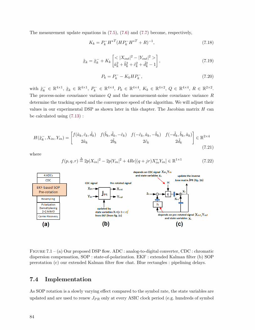
The measurement update equations in (7.5), (7.6) and (7.7) become, respectively,

Kk = P−k H∗T (HP−k H

∗T +R)−1, (7.18)

xk = x−k +Kk

[< |Xout|2 − |Yout|2 >a2k + b2k + c2

k + d2k − 1

], (7.19)

Pk = P−k −KkHP−k , (7.20)

with x−k ∈ R4×1, xk ∈ R4×1, P−k ∈ R4×4, Pk ∈ R4×4, Kk ∈ R4×2, Q ∈ R4×4, R ∈ R2×2.The process-noise covariance variance Q and the measurement-noise covariance variance Rdetermine the tracking speed and the convergence speed of the algorithm. We will adjust theirvalues in our experimental DSP as shown later in this chapter. The Jacobian matrix H canbe calculated using (7.13) :

H(x−k , Xin, Yin) =[f(ak, ck, dk) f(bk, dk,−ck) f(−ck, ak,−bk) f(−dk, bk, ak)

2ak 2bk 2ck 2dk

]∈ R2×4

(7.21)where

f(p, q, r) ∆= 2p|Xin|2 − 2p|Yin|2 + 4Re[(q + jr)X∗inYin] ∈ R1×1 (7.22)

Figure 7.1 – (a) Our proposed DSP flow. ADC : analog-to-digital converter, CDC : chromaticdispersion compensation, SOP : state-of-polarization. EKF : extended Kalman filter (b) SOPprerotation (c) our extended Kalman filter flow chat. Blue rectangles : pipelining delays.

7.4 Implementation

As SOP rotation is a slowly varying effect compared to the symbol rate, the state variables areupdated and are used to renew JPR only at every ASIC clock period (e.g. hundreds of symbol

84

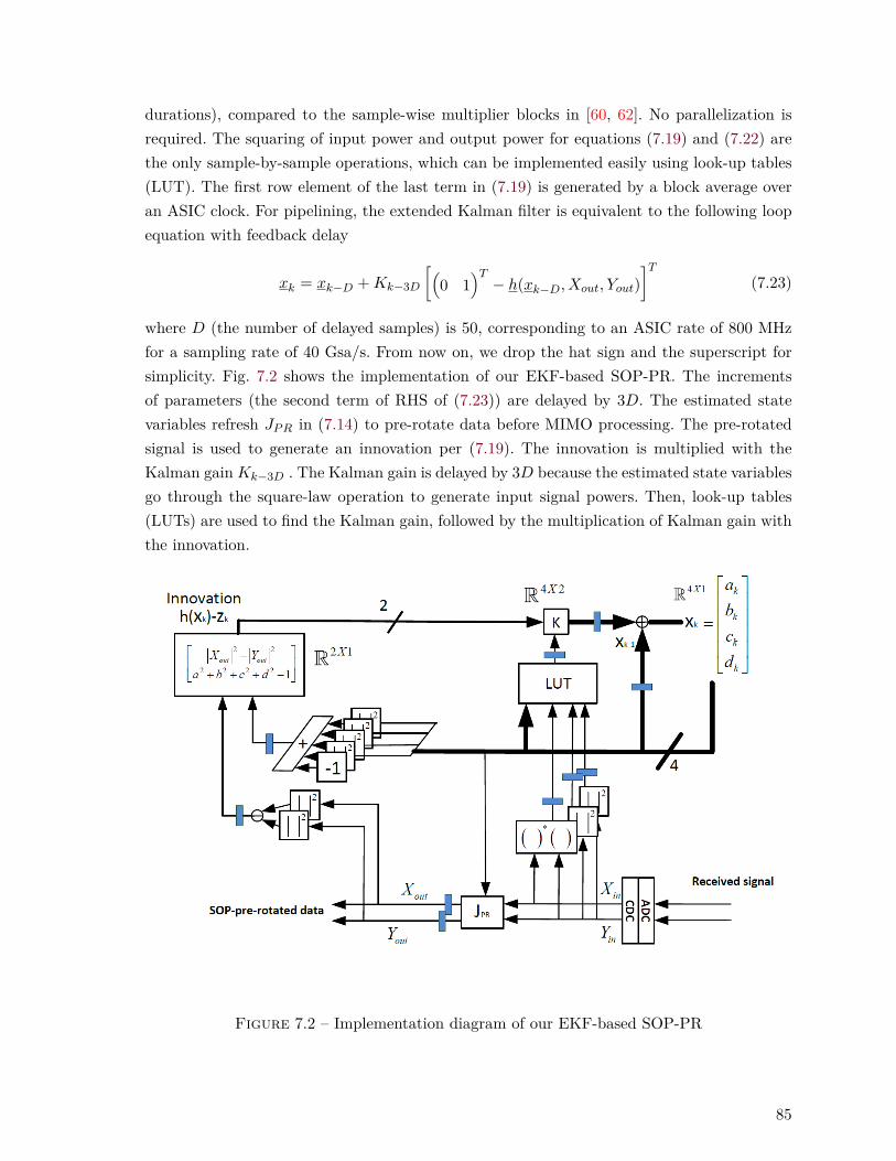
durations), compared to the sample-wise multiplier blocks in [60, 62]. No parallelization isrequired. The squaring of input power and output power for equations (7.19) and (7.22) arethe only sample-by-sample operations, which can be implemented easily using look-up tables(LUT). The first row element of the last term in (7.19) is generated by a block average overan ASIC clock. For pipelining, the extended Kalman filter is equivalent to the following loopequation with feedback delay

xk = xk−D +Kk−3D

[(0 1

)T− h(xk−D, Xout, Yout)

]T(7.23)

where D (the number of delayed samples) is 50, corresponding to an ASIC rate of 800 MHzfor a sampling rate of 40 Gsa/s. From now on, we drop the hat sign and the superscript forsimplicity. Fig. 7.2 shows the implementation of our EKF-based SOP-PR. The incrementsof parameters (the second term of RHS of (7.23)) are delayed by 3D. The estimated statevariables refresh JPR in (7.14) to pre-rotate data before MIMO processing. The pre-rotatedsignal is used to generate an innovation per (7.19). The innovation is multiplied with theKalman gainKk−3D . The Kalman gain is delayed by 3D because the estimated state variablesgo through the square-law operation to generate input signal powers. Then, look-up tables(LUTs) are used to find the Kalman gain, followed by the multiplication of Kalman gain withthe innovation.

Figure 7.2 – Implementation diagram of our EKF-based SOP-PR

85

7.5 Performance Analysis

7.5.1 Experimental Setup

The performance of our proposed DSP is examined using the experimental setup shown inFig. 6.5. A 32 Gbaud DPQPSK signal was generated by a polarization multiplexing emulator(dashed, orange), with laser sources of 10 kHz linewidth. A polarization synthesizer (AgilentN7786B) was used to rotate the SOP of the transmitted signal at 50 kHz. After passingthrough an erbium doped fiber amplifier (EDFA) and a 40 km standard single-mode fiber(SMF), the received signal was coherently detected by an integrated coherent receiver havinga bandwidth of 22 GHz. The signal was captured by a sampling scope at 40 GSa/s withlimited (16 GHz) bandwidth.

7.5.2 Offline DSP

For offline DSP, we followed the DSP flow in Fig. 7.1 to perform CD compensation first. Weapplied our proposed EKF-based SOP-PR (operated at an ASIC rate of 800 MHz) directlybefore resampling. At this point, we looked into the results of the CT tracking performance,as explained in the next paragraph. To see the application of SOP pre-rotation, we performedretiming and resampling to 2 samples per symbol, followed by polarization demultiplexing(using our proposed reduced-complexity MIMO in Chapter 6), phase recovery, detection andbit error counting.

In order to compare the clock tone magnitude with and without KF-based SOP-PR (im-portance of SOP-PR), we resampled the signal to 2 samples per symbol and extracted theclock tone using frequency-domain (FD) Godard timing phase estimation (TPE) over 1000samples [57]. Please refer to Appendix G for Godard TPE. The results of the CT trackingperformance are shown in Fig. 7.3, while those of the BER performance using our previouslypropsoed reduced-complexity MIMO are shown in Fig. 7.4.

7.5.3 Experimental Results

Our experimental results were generated based on a polarization-scrambled (at a speed of50 kHz) 32 GBaud DP-QPSK signal. The covariance matrices for process noise Q and formeasurement noise R are set via trial and error to 0.5 I4 and 5000 I2, respectively. Thephysical meanings of these two parameters are related to the convergence speed and thetracking bandwidth of the algorithm, which was well explained in [63]. However, for largesignal distortion (refer to our case where 32 GBaud QPSK was detected by a 16 GHz receiver),we had to resort to a trial and error on our measurement. We chose values for these twoparameters to achieve a stable level of clock tone magnitude with short convergence time, asshown in Fig. 7.3b. The initial state is set to [1 0 0 0 ]T .

86

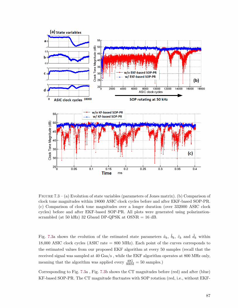
Figure 7.3 – (a) Evolution of state variables (parameters of Jones matrix). (b) Comparison ofclock tone magnitudes within 18000 ASIC clock cycles before and after EKF-based SOP-PR.(c) Comparison of clock tone magnitudes over a longer duration (over 332000 ASIC clockcycles) before and after EKF-based SOP-PR. All plots were generated using polarization-scrambled (at 50 kHz) 32 Gbaud DP-QPSK at OSNR = 16 dB.

Fig. 7.3a shows the evolution of the estimated state parameters ak, bk, ck and dk within18,000 ASIC clock cycles (ASIC rate = 800 MHz). Each point of the curves corresponds tothe estimated values from our proposed EKF algorithm at every 50 samples (recall that thereceived signal was sampled at 40 Gsa/s , while the EKF algorithm operates at 800 MHz only,meaning that the algorithm was applied every 40G

800M = 50 samples.)

Corresponding to Fig. 7.3a , Fig. 7.3b shows the CT magnitudes before (red) and after (blue)KF-based SOP-PR. The CT magnitude fluctuates with SOP rotation (red, i.e., without EKF-

87

based SOP-PR). During the acquisition stage (the first 1000 ASIC clocks), the two curves (redand blue) overlap. Once EKF adapts to a correct SOP, our proposed EKF-based SOP-PRrestores the CT magnitude and maintains the CT magnitude at a high level. This helps reducejitter and eliminate system failure of coherent receivers. To shorten initial convergence time,we can simply use blind SOP search proposed in Chapter 6.3 to initialize the state variables(not shown here). Fig. 7.3c is similar to Fig. 7.3b, but showing the clock-tone magnitudesbefore and after EKF-based SOP-PR over a longer duration (over 332000 ASIC clock cycles,or 332000× 1

800MHz = 0.415 ms ).

To show the advantage (application) of our proposed EKF-based SOP-PR, Fig. 7.4 shows theBERs versus time of our proposed reduced-complexity MIMO filter taps (with Ncross = 7,proposed in Chapter 6) without (red) and with (blue) EKF-based SOR-PR. To verify that ourproposed EKF can pre-rotate SOP correctly, the evolution of the BER values was shown at afixed OSNR of 16 dB, measured every minute, taken over 120 minutes, i.e. each curve consistsof 120 points. At each point, 80000 DP-QPSK symbols were used to calculate a BER value.Our proposed technique results in a lower BER (below 1e-3), because the EKF tracks theSOP rotation, and JPR coarsely reject the SOP change. Therefore, the cross taps of MIMOcan be significantly reduced.

Fig. 7.5 shows the averaged BERs (over 120 minutes) versus OSNRs of reduced-complexityMIMO filter taps without (red) and with (blue) EKF-based SOR-PR, compared with thebest performance given by a full-complexity MIMO (black). The BER value at each OSNRwas calculated by using all 120 captures within 120 minutes, i.e., 120 × 80000 = 9.6 millionDP-QPSK symbols. Our proposed technique improves the OSNR penalty at BER of 1e-3by 1.5 dB for reduced-complexity MIMO filter, but degrades by 0.5 dB compared to a full-complexity MIMO. This extra link budget is counter-balanced by the reduced complexity ofour proposed algorithm, and is still within the working OSNR range in short-reach scenarios.

7.6 Conclusion

In this chapter, we have extended our work in Chapter 6 to use SOP pre-rotation to solve theproblems of the conventional MIMO. The difference in this chapter is that we have proposed alow complexity discrete-time extended Kalman filter operated at ASIC rates to track the Jonesmatrix of the inverse of an optical channel (the polarization effects) based on minimizationof s1. Compared to the blind SOP search proposed in Chapter 6, the extended Kalman filtercan save memory and redundant computations.

In Chapter 6, an experimental demonstration was performed for various static SOPs, follo-wed by a complexity-performance trade-off to emphasize the importance of SOP-PR for ourproposed reduced-complexity MIMO for short-reach scenarios. This "proof-of-concept" sho-wed that the weakened clock tone can also be restored at the same time for various SOPs,

88

Figure 7.4 – Comparison of bit error rates (measured every minute) of using reduced-complexity MIMO filter taps (Ncross = 7) proposed in Chapter 6 with and without EKF-based SOP-PR. All plots were generated using polarization-scrambled (at 50 kHz) 32 GbaudDP-QPSK at OSNR = 16 dB.

Figure 7.5 – Comparison of bit error rates versus OSNRs of using reduced-complexity MIMOfilter taps (Ncross = 7) in Chapter 6 with and without EKF-based SOP-PR, and using a full-complexity MIMO with EKF-based SOP-PR. All points were generated using polarization-scrambled (at 50 kHz) 32 Gbaud DP-QPSK

suitable for applications for burst-mode receivers in short-reach scenarios. In this chapter, ourexperimental demonstration focused on the performance of our proposed DSP in clock tonerecovery. We tested our proposed SOP tracking and previously proposed reduced-complexityMIMO with dynamic SOPs (scrambled at 50 kHz).

Our experimental results of a polarization-scrambled 32 Gbaud DP-QPSK system show that

89

the clock tone magnitude can be restored by our proposed extended Kalman-filter-based SOPpre-rotation at a 800 MHz ASIC rate. This avoids the clock tone loss due to the polarizationeffect of the optical channel, and enhances the bit-error rate performance of using a reduced-complexity MIMO for digital polarization demultiplexing.

90

Chapitre 8

Conclusion

In this thesis our first contribution was experimentally showing, for the first time, that Te-raXion’s narrow-linewidth lasers gives BER improvement in real-time phase recovery (paralleland pipelined decision-directed maximum likelihood estimation ) that consists of a feedbackloop. Using a fiber Bragg grating suppresses the frequency noise spectral level of narrow-linewidth semiconductor lasers such as external cavity lasers or integrated tunable laser as-semblies. The laser source permits greater parallelization, e.g., increase from 16 to 20, toreduce the hardware processing rate from 312.5 to 250 MHz. We pointed out that the use oflaser linewidth to predict system performance is no longer appropriate to quantify laser phasenoise for a laser with frequency noise suppression. We suggested the use of frequency noisepower spectral density levels to quantify the impact of laser phase noise for real-time phasetracking with feedback delay. Offline experimental demonstrations often neglect feedback de-lay.

Hardware parallelization and pipelining are required to implement real-time systems, but im-pose delay on the feedback path of the real-time decision-directed phase recovery, reducingits tracking bandwidth. For current electronics (i.e. ASIC rates between 200 MHz and 400MHz are used because of optimal power consumption [29]), we found that the laser frequencynoise between 10 MHz and 100 MHz affects the BER performance of real-time phase tra-cking for a single-polarization, single-carrier 5 Gbaud 64-QAM system. We expect that thisconclusion also holds for higher symbol rates as well, as a higher symbol rate requires higherparallelization in the current CMOS technology.

Our second contribution was pointing out, for the first time, that the standard frequencyoffset compensation algorithm could cause real-time phase tracking failure for 64-QAM inthe presence of sine tones in laser sources below 1 MHz. We demonstrated experimentallythe impact of sinusoidal laser phase noise on phase recovery in the presence of paralleliza-tion and pipelining delay. Our demonstration applied parallel and pipelined DD-MLE to asingle-polarization, single-carrier 5-Gbaud 64-QAM system, taking into account the popu-

91

lar NDA-FFT for frequency-offset compensation and static equalization. We experimentallyinvestigated, for the first time, the ranges of the FM amplitude and FM frequency of la-ser sources to avoid real-time phase tracking failure. Together with our simulation results,we found that the frequency modulated (FM) amplitude and FM frequency of laser sourcesshould be smaller than 1.5 MHz and 75 kHz, respectively, to avoid tracking failure.

Our third contribution was proposing a novel DSP technique to solve the problems of conven-tional MIMOs for polarization demultiplexing and reducing the power consumption in short-reach coherent communications systems, where DGD is present but not prominent. We pro-posed a very coarse SOP pre-rotation before MIMO using an inverse Jones matrix basedon the minimization of only a single Stokes parameter (s1) via a blind SOP search. ThisSOP pre-rotation can coarsely reject the polarization crosstalk before the subsequent polari-zation demultiplexing DSP. It brings advantages compared to the conventional MIMO-FIRapproaches : only a single Stokes parameter instead of all three Stokes parameters, greatlyreducing the computational effort for estimating SOP compared to other Stokes-space ap-proaches. It avoids the problem of long MIMO convergence and singularity for certain SOPs,which makes the DSP very suitable to burst-mode receivers normally in packet-switching ba-sed short-reach or metro networks. As the SOP pre-rotation reduces polarization coupling, weare then at liberty to reduce the number of MIMO cross-taps (the off-diagonal components ina Jones matrix), leading to a significant reduction in number of MIMO-FIR complex multi-pliers. The SOP pre-rotation also brings the benefit of restoring clock tones for timing phaseestimation (TPE) even before MIMO. The hardware overhead for coarse SOP estimation iseasily counter balanced by savings in MIMO complexity. We have also experimentally pre-sented a tradeoff between hardware reduction and performance degradation in the presenceof residual chromatic dispersion for short-reach applications.

Our fourth contribution was proposing a low-complexity discrete-time extended Kalman filter(EKF) minimizing resultant s1 in order to track depth required in our proposed blind SOPsearch in our third contribution. Our proposed algorithm is updated only at every ASIC clockperiod and can be applied to real-time data. We experimentally showed that this EKF allowsus to keep maintaining a good clock tone magnitude level (which is important for timing phaseestimation), has significant complexity reduction compared to the existing sample-wise multi-plier blocks in timing-phase estimation algorithms, and preserves all the advantages mentionedin our third contribution, such as avoiding the singularity problem and long convergence ofconventional MIMO, and helps reduce the subsequent MIMO-filter taps.

8.1 Future Work

Coherent systems usually have higher performance than other systems, but power consump-tion is always a concern for implementing DSP on ASIC chips, especially for metro networks

92

and short-reach applications where the device density (device per user) is high. Crivelli etal. [5] summarized, for the first time, the power consumption of different DSP stages in along-haul DP-QPSK coherent chip : the highest power consumption of a chip is due to thebulk CD compensation consumes (11 W), while the second highest power consumption is dueto the equalization using MIMO-FIR (6.95 W). Undoubtedly, MIMO-FIR becomes a majorconsumption in short-reach systems where CD is small, and our DSP designs in Chapters 6and 7 are to further reduce the power consumption of digital coherent receivers for short-reach applications. However, the reduction of power consumption is only the calculation ofthe number of complex multiplications used in our new DSP, which is a crude evaluationonly. The true power consumption varies with implementation. One of our future work is toexamine the performance of our DSP design in Chapters 6 and 7 via implementation in FPGAexperimentally before the design is realised in ASIC for further circuit optimization for powersaving.

It is well-known that the convergence time is determined mainly by MIMO-FIRs in burst-modereceivers for packet-switching applications in short reach systems [33]. Reducing convergencetime helps enhancing the chip power efficiency for useful packet content. We may calculatethe acquisition times required by our proposed DSP in Chapters 6 and 7 for different SOPsso that the duration of headers can be tailored made for each data packet.

Dependence on modulation format is also a concern of designing DSP. Our proposed DSP for32 Gbaud DP-QPSK (100 Gbps system) relies on the signal representation of dual-polarizationsignals in Stokes space, forming a lens object on the Poincaré sphere. Higher-order modulationformats are more susceptible to receivers’ electrical bandwidth, resulting in a distorted lensobject causing inaccurate SOP estimate. One may suggest to employ 16 Gbaud DP-16-QAMto achieve 100 Gbps systems, as the reduced symbol rate helps saving parallelization and thuspower consumption. One of our future work is to make our SOP estimate generic to 16-QAMor higher.

93

Annexe A

Phase Estimation and PhaseTracking

In this appendix, we discuss the definition of phase estimation and phase tracking in a strictersense. The unknown quantity or variable of a system that one desires to find out is calleda parameter. This parameter may be random in nature, and therefore statistical estimationmethods are required. For example, in Chapter 2 and 3, the parameter of concern is the laserphase noise.

A.1 Theoretical viewpoint

There are two kinds of knowledge about a random process to understand its nature. Firstly,the ensemble statistics that give the probability distribution of the random process ata certain time instant, i.e., a random variable only. Examples are mean and variance of adistribution.

Secondly, as a random experiment proceeds with time, i.e., the same experiment is repeated,the randomness may be the same or different at different time instants 1. This refers to arandom process. Usually, we are interested in the relationship between the repeated experi-ments (i.e., between the random variables at different time instants), as we aim at describingthe randomness in the past or predicting what happens in future. The repeated experimentsat different time points can only be either independent to, or correlated with each other,which correspond to independent random processes, and Markov processes, respectively. Oureffort lies on finding out the process properties (in a continuous sense) or the time se-ries properties (in a discrete sense) which gives the temporal dynamics or system dynamicsthat governs how a random process behaves, i.e., the correlation between the repeated expe-

1. For example, the stock market behaves differently in times slots from 9 and 10 am and from 10 to 11am.

95

riments at different time instants. For linear systems, the temporal dynamics can usually berepresented by linear differential equations.

Strictly speaking, one has to find out all the higher-order joint moments of the random pro-cesses at different time points, in case that the random process shows time-varying statistics,i.e., non-stationary random process. In particular, for a second-order stationary (or calledwide-sense stationary) random process, one can characterize a random process using stochas-tic tools such as autocorrelation function and power spectral density to capture its propertiesbased on its ensemble statistics and time-series properties.

In mathematics, we define random variables to be estimated as parameters if their statisticalproperties is time-invariant. Time-varying parameters are usually called signals [47], which arerandom processes. Parameter estimation only requires the knowledge of the ensemble sta-tistics of a random parameter to be estimated. In Chapter 2, one assumes that the parameter,i.e., laser phase noise, is approximately a constant over a temporal observation window, andphase estimation is performed using averaging to obtain the mean of the phase variationover a certain time. Signal tracking requires the knowledge of both the ensemble statisticsand the temporal dynamics (time-series properties) of a random process to be estimated. Infact, in Chapter 2, if one wishes to have an optimal estimation of the signal, i.e., time-varyinglaser phase noise (following Brownian motion), phase tracking should be performed by ma-king use of the properties of the Wiener process. Wiener filter and Kalman filter are twotypical examples used for optimal signal tracking [47].

For example, the conventional Viterbi-Viterbi algorithm 2 requiring only a moving averagebelongs to the class of phase estimation because phase noise dynamics are not required. On theother hand, Viterbi-Viterbi algorithm followed by aWiener filter [23] belongs to phase trackingbecause the phase noise dynamics are assumed to be a first-order difference equation (randomwalk). Intuitively, as phase tracking requires more knowledge about a random process to beestimated, phase tracking can give a more "optimal" phase estimate than phase estimation.

A.2 Commercial Systems

The techonology of optical coherent communications has been widely deployed, and publica-tions from both academia and industries are becoming more industrial-oriented. For simplicity,phase estimation usually refers to the process of estimating a time-varying phase via movingaverage in a feedforward structure (without feedback). Phase tracking usually refers to theprocess of estimating phase with feedback, using the previous estimated phase to update orassist the current phase estimation.

2. Recall that Viterbi-Viterbi algorithm removes the data information by taking Mth power of the receivedsignal, and therefore only phase is left as an unknown parameter. Please refer to Section 2.2.2.

96

Annexe B

Laser Phase Noise

In this appendix, we will first give the mathematical definitions of frequency noise and Wienerphase noise. We will see that Wiener phase noise is the integration of white Gaussian frequencynoise. We will define the phase noise increment as well as power spectral density of the opticalfield. Phase noise increment is important for evaluating field power spectral density. In SectionF.1, we make use of phase noise variance or field power spectral density for estimating laserlinewidths. The most important equation in this appendix is B.14, especially for Chapter 2and 3. We will see that the discretized Wiener process is described by a Gaussian randomwalk process. Finally, the procedures for generating Wiener phase noise in Matlab will becovered.

Definition of Frequency Noise

First, we define ∆f(t) as frequency noise of a laser source, an independent and identicallydistributed (i.i.d) zero-mean Gaussian random process with a variance of σ2

∆f . The randomprocess ∆f(t) has an autocorrelation function

R∆f (r, s) = E [∆f (r) ∆f (s)] = σ2∆fδ (r − s) , (B.1)

where r and s are time variables, E [·] refers to the ensemble average (expectation) withrespect to the joint distribution of ∆f (r) and ∆f (s), δ (r − s) is the Dirac delta function.When r = s, (B.1) becomes

R∆f (r, r) = E [∆f (r) ∆f (r)] = σ2∆f , (B.2)

97

which is the variance of the random variable ∆f . 1 The power spectral density (PSD) S∆f (f)of the random process ∆f is

S∆f (f) = σ2∆f , ∀f. (B.4)

Since the PSD is flat, the corresponding Gaussian random process is called a white Gaussianprocess.

Definition of Wiener Phase Noise

The frequency of a signal is the derivative of the phase, hence phase noise can be written as

θ (t) = 2π∫ t

0∆f (s) ds. (B.5)

This process is non-stationary. For instance, it has a variance σ2∆f t that is a function of

absolute time t (p. 517 in [14]). Since integration is a linear operation, phase noise is alsoa Gaussian process. Strictly speaking, one should not comment directly on the variance ofWiener phase noise without defining a reference time point (where Wiener process starts).The value σ2

∆f t refers to the variance of Wiener phase noise from t = 0 up to time t.

Definition of Phase Noise Increment

From (B.5), we define the phase noise increment as

θτ (t) ∆= θ(t+ τ)− θ(t) = 2π∫ t+|τ |

t∆f(s)ds. (B.6)

The phase noise increment over the time interval τ is a zero-mean Gaussian random process 2

with variance :

σ2θτ = E

[|θτ |2

]= E

{2π∫ t+|τ |

t∆f(s)ds

}2 = (2π)2

∫ t+|τ |

tds

∫ t+|τ |

tdu · σ2

∆fδ (s− u) .

(B.7)Since

∫ t+|τ |t δ (s− u) du = 1 for t ≤ s ≤ t+ |τ | and zero for elsewhere, we have

σ2θτ = (2π)2σ2

∆f

∫ t+|τ |

tds = (2π)2 σ2

∆f |τ | . (B.8)

Therefore, the autocorrelation function of phase noise increment depends only on time intervalτ and not absolute time t, implying that the random process is WSS, and the Gaussian processθτ (t) is stationary. Thus, θτ (t), θτ (t+τ), θτ (t+2τ) are i.i.d., i.e., Wiener process has stationaryindependent increments.

1. As the autocorrelation is only a function of the lag τ , we can write

R∆f (τ) = σ2∆fδ (τ) , (B.3)

meaning that the random process is wide-sense stationary (WSS). As ∆f (t) is a Gaussian random process, itis not only WSS but also stationary. As the process is WSS, we can apply Wiener-Khintchine theorem to findits power spectral density (PSD) by taking the Fourier transform of the autocorrelation with respect to τ .

2. θτ (t) is a Gaussian random process because of the linearity of integration

98

Power Spectral Density of Optical Field

We define the optical field of a laser source with constant amplitude and phase noise θ (t) as

A(t) ∆= ejθ(t). (B.9)

Its autocorrelation function between two samples at time t and time s is

RA (t, s) = E [A(t)A∗(s)] = E[ejθ(t)e−jθ(s)

], (B.10)

where E [·] refers to the ensemble average with respect to the joint distribution of the randomvariables θ (t) and θ (s) at time instant t and s respectively. Let t = t+ |τ | , s = t, using (B.8)and the characteristic function for zero-mean Gaussian random variable, the autocorrelationbecomes

RA (t+ |τ | , t) = RA (τ) = e−2π2σ2∆f |τ |, (B.11)

which is a function of time interval τ only and therefore the optical field of the laser sourceis WSS. The exponential autocorrelation [14] results in a well-known Lorentzian PSD, i.e.

SA (f) =∫ ∞−∞

RA (τ) e−j2πfτdτ =σ2

∆f(πσ2

∆f)2 + f2

. (B.12)

The linewidth ∆ν of a laser source is defined as the 3-dB width (two-sided) of the Lorentzianfield PSD [7] :

∆ν = 2πσ2∆f = 2πS∆f (f). (B.13)

Note that the above linewidth definition is only for laser sources having pure Wiener phasenoise, or equivalently white frequency noise, satisfying (B.4). (B.12) is not valid for coloredfrequency-noise PSD as discussed in Chapter 3. For Wiener phase noise, the linewidth can befound directly by referring to the level of frequency-noise PSD, and the phase noise incrementover time T is thus, by substituting (B.13) into (B.8),

σ2θT

= E[|θ(t+ T )− θ(t)|2] = 2π∆νT. (B.14)

Discretization of Wiener Phase Noise

To perform digital signal processing on measurement data or to conduct simulation, oneneeds to consider discretization random process rather than continuous process. Here wewould clarify how we deal with the discretized phase noise.

Wiener process in (B.5) means simply a first-order Markov process that obeys Langevinequation with an indepedent Gaussian noise source. (B.5) can be discretized as a sum process :

θk = 2πk−1∑m=0

fm, (B.15)

99

where k is the time index taking every sampling period Ts, fk is the discretized frequencynoise, θ0 = 0 defines the starting point, θk = θ(kTs), fk = f(kTs). In fact, (B.15) is a Gaussianrandom walk :

θk = θk−1 + 2πfkTs. (B.16)

Ideally, frequency noise ∆f(t) corresponds a phase noise increment θτ (t) in (B.6) when τ ap-proaches zero, i.e. ∆f(t) = limτ→0

θτ (t)2πτ . In practice or in simulation, τ is limited by sampling

duration Ts = 1/BWs, where BWs is the sampling rate or the simulation bandwidth. There-fore, the discretized frequency noise becomes fk = θTs (kTs)

2πTs , and, using (B.8), has a variance of

Σ2∆f , where Σ2

∆f =(2π)2σ2

∆fTs

(2πTs)2 =σ2

∆fTs

. This shows that the discretized frequency noise requiresa rescaling to guarantee a proper variance. In Matlab, the discretized frequency noise shouldbe generated using the following procedures :

1. generate an i.i.d. zero-mean normal vector Uk ;

2. specify the value of laser linewidth ∆ν ;

3. calculate the variance using (B.13), i.e. σ2∆f = ∆ν

2π

4. multiply the vector with Σ∆f to make sure that the overall variance of the vector is stillσ2

∆f/Ts. The resultant vector, the discretized frequency noise vector, is fk

=√

∆ν2πTsUk ;

5. using (B.16), the discretized Wiener phase noise can be generated via θk = θk−1 + νk,where νk =

√2π∆νTsUk.

100

Annexe C

Reduction in Power Consumptiondue to Parallelization andPipelining

This section reviews the reduction in power consumption of CMOS circuits due to pipeliningand parallelization [[42], Ch. 3 and 10], discussed in Chapter 2. First, the power consumptionPCMOS of a CMOS (complementary mental-oxide-semiconductor) circuit can be approxima-ted by

PCMOS = CtotalV2

0 fclk (C.1)

where Ctotal is the total capacitance of the circuit, V0 is the supply voltage, and fclk is theclock frequency of the circuit. It is assumed that the capacitance of multipliers, slicers andlookup tables dominates those of adders and pipelining registers. Second, the critical path(defined as the minimum time required for processing the next new sample [[42], Ch. 3]) islimited by the propagation delay related to the charging and discharging of the CMOS gateand stray capacitances. Thus, the minimum allowed clock period of the processor Tproc canbe expressed as

Tproc = CchargeV0

k(V0 − Vt)2 (C.2)

where Vt is the CMOS threshold voltage, and k is a process parameter depending on thematerial and geometry applied in the CMOS technology [[67], Ch. 2], and Ccharge is thecapacitance to be charged or discharged in a single clock cycle. The interconnect capacitanceusually dominates the CMOS gate capacitance, and appears as the major capacitances (e.g.multipliers) within a critical path. For a fair comparison of power consumption between serialprocessing and parallel processing (with different parallelization level P ), we assume that theparallel DD-PR is pipelined with an identical number of registers in each parallel rail as that

101

of the serial pipelined DD-PR. Please note that fine grain pipelining [[42], p. 69] for multipliersor for lookup tables and bit-level pipelining [[42], p. 482] are not considered here.

For pipelining, the insertion of d pipelining registers reduces the original physical distancewithin a critical path by d times (where d is the number of pipelining registers as defined inChapter 3). Thus, the charging capacitance is also reduced by d times because of the reducedcoverage of interconnect on the grounded substrate [42], Ch. 6], while the overall capacitanceof the circuit is not changed significantly by the addition of pipelining registers. The charging-capacitance reduction allows a faster transition (or a shorter rise-time because of a smaller RCconstant), which equivalently reduces the supply voltage from V0 to βV0 (for β < 1) within aclock duration, and the propagation delay Tpd,s,pip for pipelined serial processing is

Tpd,s,pip = Ccharge,pip (βV0)k(βV0 − Vt)2 (C.3)

where Ccharge,pip is the charging capacitance after pipelining.

For parallel and pipelined processing, the same serial pipelined DD-PR is duplicated in parallelby P times, leading to P -folded increase in the total capacitance in the circuit, while thecharging capacitance of each parallel rail, and thus the propagation delay Tpd,p,pip remainsthe same as that of the serial pipelined processing :

Tpd,p,pip = Tpd,s,pip = Ccharge,pip (βV0)k(βV0 − Vt)2 (C.4)

since the processing rate of each parallel rail is P times slower than the original processingrate. Using (C.2) and (C.4)), Tpd,p,pip becomes

Ccharge,pip (βV0)k(βV0 − Vt)2 = P

CchargeV0

k(V0 − Vt)2 (C.5)

By solving the quadratic equation in β in (C.5) and using (C.1), the power consumption forparallel and pipelined processing can be calculated as

PCMOS,p,pip = C′totalβ

2

CtotalPPCMOS (C.6)

Taking V0 = 5 V, Vt = 0.6 V, d = 4, Ccharge,pip = Ccharge/d ,C ′charge = Ccharge × P , thepower consumption for P = 16 and P = 20 are 2.71% and 2.54% of the original circuit,respectively, leading to a 6.3% reduction in power consumption for performing DD-PR whenthe parallelization level P increases from 16 to 20.

102

Annexe D

Reduction of Tracking Bandwidth

This appendix supplements Section 2.5. Intuitively, lower FN-PSD level results in a smallerparallel phase tracking error. In this appendix, we will first discuss the bandwidth reductionof parallel digital feedback loop in more detail based on the implementation form of decision-directed maximum likelihood estimation.

The discrete loop equation for describing parallel DD-MLE is derived based on [75]. Assu-ming that the phase tracking is performed after perfect equalization and frequency offsetcompensation, the phasor estimate V [[75], (3)] of parallel DD-MLE in Fig. 2.6 is

V = e−jθk−i+1 =k−dP∑

m=k−(d+1)P+1

dm(d∗me−jθm + n∗m)∣∣∣dm∣∣∣2 (D.1)

where θk−i+1 is the phase estimate at time index k − i + 1, i is the parallelization channelindex taking from 1 to P , the subscript m refers to time index, θm is the true phase, dm isthe complex transmitted QAM signal, nm is the complex AWGN, dm is the decision symbolof QAM signals.

The LHS of (D.1) corresponds the phase estimates at time indices k−P + 1, . . . , k, while theRHS of (D.1) corresponds to the received symbols at time indices k− (d+1)P +1, . . . , k−dPrequired to construct the phase estimates. For each round of time interleaving, a commonphase estimate is shared by all P channels. For i = dP, . . . dP + P − 1, θk−(d+1)P+1 = · · · =θk−dP . Therefore, for the (dP )th round of time interleaved input signals, the common phaseestimate can be factorized out from the summand. Assuming small phase tracking error, suchthat slicers (decision device) give correct decisions, (D.1) becomes

e−jθk−i+1 = e−jθk−dP+1k−dP∑

m=k−(d+1)P+1(e−j(θm−θm) + n∗1,m) (D.2)

where the noise term n∗1,m∆= n∗me

jθm/d∗m is rescaled in magnitude by d∗m, and is rotated byboth phase estimate θm and the phase of d∗m. For smaller tracking error, the summand term

103

in (D.2) becomes

k−dP∑m=k−(d+1)P+1

(e−j(θm−θm) + n∗1,m) =k−dP∑

m=k−(d+1)P+1[1− j(θm − θm) +Re(n∗1,m) + jIm(n∗1,m)]

(D.3)

For high SNR,the unwrapped phase(D.2) becomes

θk−i+1 = θk−dP−i+1 + 1P

k−dP∑m=k−(d+1)P+1

(θm − θm)− 1P

k−dP∑m=k−(d+1)P+1

Im(n∗1,m) (D.4)

Note that (D.4) holds for all P channels during each round of time interleaving, as all channelsshare the same phase estimate. Both the second and the third terms of (D.4) refer to theincrement of the discrete loop equation. The second term of (D.4) is the weighted sum ofphase errors taken from k − dP − P + 1 to k − dP , with the mth weight equal to the mth

received symbol energy. Similarly, the third term of (D.4) is the weighted sum of the imaginarypart of n∗1,m taken from k − dP − P + 1 to k − dP (for high SNR [75]), with the mth weightequal to the mth transmitted symbol energy. These two terms are scaled down by the totalsymbol energy within the time duration from dP − P + 1 to k − dP .

104

Annexe E

Frequency Noise Power SpectrumDensity

This section supplements Chapters 2 and 3, giving the origin of the f2-curve at high frequen-cies in the additive white Gaussian noise (AWGN) FN-PSD in Fig. 2.8. While observable inseveral references on laser characterization, a thorough analysis is infrequent. Chen et al. [3]attributed such a f2-curve to optical ASE noise and fiber nonlinearity. However, our previouswork in [[40], Fig. 2] experimentally showed the f2-curve in the absence of fiber transmissioncontradicting this explanation, and suggesting that the f2-curve originates from the electricalnoise of the coherent receiver. To our best knowledge, Leeson [34] first illustrated that thef2-curve on FN-PSD is due to white phase noise introduced by thermal noise of electrical os-cillators (which appeared as a flat noise floor in PNPSD), and approximated the level of thePN-PSD noise floor using thermal-noise parameters. The small modification for the PN-PSDnoise floor can be made by referring to the exact PDF for white phase noise given by Fu andKam [12].

After coherent detection, the measurement appears as a complex phasor in baseband

rk = Aejθk + nk, (E.1)

where θk is the total laser phase noise, nk is the zero-mean white Gaussian electrical noise ofcoherent receiver, with a variance of σ2 contributed by thermal noise and LO-noise beating,A is the real amplitude of measurement phasor rk.

The field PSD of rk consists of a Lorentzian shape near the zero frequency caused by theBrownian phase noise, and a flat floor due to electrical noise covering elsewhere in the fieldPSD. This two-sided field PSD of white Gaussian noise can be expressed as

No = σ2/BW2−sided (E.2)

where BW2−sided is the two-sided bandwidth of the spectrum, or the sampling rate of the

105

ADC (real-time oscilloscope), corresponding to the simulation bandwidth 1. To obtain PN-PSD, assuming that there is no phase wrapping, we take the angle of E.1

Arg (rk) = Arg[(ejθk + nk/A

)]= θk + εk (E.6)

where εk is the white phase noise. Applying geometric approach on complex plane for (E.1)shown in [[12], Fig. 1], the exact probability distribution function (pdf) of white phase noiseθ depends on measurement, showing a zero-mean Tikhonov distribution with a variance ofσ2/(2|rk|A) [[12], (18)]. For SNR larger than 10 dB, the pdf can be approximated well by azero-mean Gaussian distribution with a variance of σ2/(2A2) [[12], (17)], where the factor of 1

2can be thought as the equal contribution of in-phase and quadrature-phase noise components.Thus, the phase-noise PSD for white phase noise is given by No/(2A2).

In DSP, we obtain frequency noise by differencing two consecutive phases [[25], (2)], andthe FN-PSD, which is the PSD of discretized frequency noise, should have a sinc squaredenvelope 2 [[25], (4)], but its effect can only be observed at high frequencies around the symbol

1. Ideally, in textbooks such as [48], one usually obtain the PSD level by referring to the magnitude of theautocorrelation of a white noise by using Wiener-Khintchen theorem, such that

S(f) = F{Noδ(τ)} = No, (E.3)

where F refers to Fourier transform. The ideal noise variance, σ2ideal, is obtained by setting τ to zero, such

that

R(τ) =∫ ∞−∞

S(f)ej2πfτdf,

σ2ideal = R(0) =

∫ ∞−∞

S(f)df.(E.4)

Obviously, σ2ideal is infinite because of the infinite bandwidth as the upper and lower bounds of the integral.

Due to finite measurement bandwidth in practice, i.e., limited by the sampling rate of the ADCs, equation(E.4) becomes

σ2 =∫ BW2−sided/2

−BW2−sided/2Nodf = NoBW2−sided, (E.5)

where σ2 is the noise variance from measurement or from simulation. It leads to the result in equation (E.2).Note that the PSD level of a white noise, No, must be the same in both equation (E.2) and equation equation(E.5). The only difference is that, from our measurement, σ2 must be finite (and thus is smaller than σ2

ideal)because of the limited bandwidth of instruments. In summary, for theoretical analysis, No = σ2

ideal, while formeasurement or for simulation, No = σ2/BW2−sided, and the values of No calculated from both theory andmeasurement must be the same.

2. As discussed in Appendix B, the sampled (discretized) frequency noise is defined as fk = θTs (kTs)2π Ts

=θ(kTs+Ts)−θ(kTs)

2π Ts. Using (B.6),

fk = 1Ts

∫ kTs+Ts

kTs

∆f(s)ds, (E.7)

where ∆f(t) is our continuous frequency noise. fk has been shown to be WSS, and therefore fk has the samePSD for any k. For simplicity, take k = 0,

fo =∫ Ts

0h(s)∆f(s)ds = h(t) ∗∆f(t), (E.8)

106

rate. Thus, the calculated (discretize) FN-PSD is assumed to be the true (continuous) FN-PSD by ignoring the envelope at frequencies below GHz. The FN-PSD can be simply derivedby multiplying f2 of the phase-noise PSD [3], i.e.

S∆f,AWGN (f)dB =[No

/(2A2

)]dB

+ 20log10f, (E.10)

which agrees with [34]. From (E.10), on the logarithmic FN-PSD, the slope of the f2-curvedoes not change as shown in Fig. 3.3 and Fig. 3.4. An increase in electrical noise only bringsup the f2-curve.

where h(t) = 1Ts

for t ∈ [0, Ts) and zero for elsewise, with a Fourier transform H(f) = e−jπfTs sinπfTsπfTs

, andtherefore the PSD of fk, FN-PSD, becomes

Sfk = sin2 πfTs(πfTs)2 S∆f , (E.9)

showing a sinc squared envelope. The 3-dB attenuation of this envelope appears at f = 14Ts = BW2−sided

4 ,which is well-above 100 MHZ (where the FN-PSD level is used for measuring linewidth of conventional lasers),i.e. Sfk ≈ S∆f for frequencies below BW2−sided

4 .

107

Annexe F

Laser Characterization

Measuring the true laser linewidth requires a coherent receiver (delayed self-homodyne co-herent detection) or an interferometric setup with direct detection (p. 180, [7]). In this ap-pendix, we will outline the techniques for linewidth measurement using a coherent receiver,to supplement Chapter 3.

F.1 Measurement Techniques for Laser Linewidth

A coherent receiver captures both real I(t) and imaginary Q(t) components of the opticalfield, and therefore we completely know the optical field in (B.9) using A(t) = I(t) + iQ(t).

To measure the linewidth using a coherent receiver, we have the following three techniques :

1. The field PSD SA (f) is found by capturing the complex electrical signal, A (t), compu-ting its autocorrelation, and taking the Fourier transform of the autocorrelation. Thenwe can fit a Lorentzian curve with a suitable linewidth to the measurement.

This method is only suitable for large laser linewidths (a few MHz or higher) becausesmall-linewidth (below MHz) lasers give sharper Lorentzian field PSD which requires ahigher FFT resolution to identity the 3-dB bandwidth of the field PSD.

Higher FFT resolution requires a longer observation window in time. However, usuallylow-linewidth laser sources contain unexpected control tones. Together with the low-frequency noise such as flicker noise (due to mechanical vibration), the Lorentzian fieldPSD peak moves around zero frequency, resulting in a much larger estimated linewidth.

2. Another method is to compute the variance of phase noise increment captured with thecoherent setup and use (B.8). The linewidth can be estimated using [(6), [55]] :

∆υ = 2πσ2∆f = 2π

[σ2θτ

(2π)2 τ

]=σ2θτ

2πτ =E[|θ(t+ τ)− θ(t)|2

]2πτ . (F.1)

109

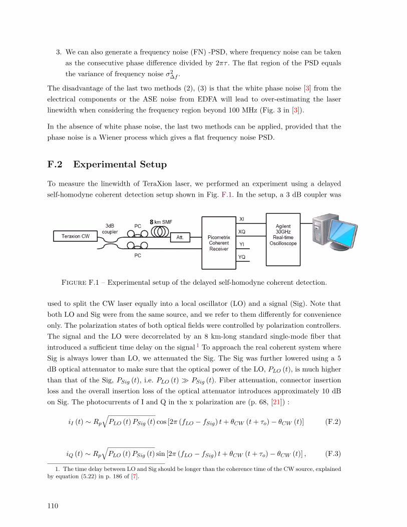
3. We can also generate a frequency noise (FN) -PSD, where frequency noise can be takenas the consecutive phase difference divided by 2πτ . The flat region of the PSD equalsthe variance of frequency noise σ2

∆f .

The disadvantage of the last two methods (2), (3) is that the white phase noise [3] from theelectrical components or the ASE noise from EDFA will lead to over-estimating the laserlinewidth when considering the frequency region beyond 100 MHz (Fig. 3 in [3]).

In the absence of white phase noise, the last two methods can be applied, provided that thephase noise is a Wiener process which gives a flat frequency noise PSD.

F.2 Experimental Setup

To measure the linewidth of TeraXion laser, we performed an experiment using a delayedself-homodyne coherent detection setup shown in Fig. F.1. In the setup, a 3 dB coupler was

Figure F.1 – Experimental setup of the delayed self-homodyne coherent detection.

used to split the CW laser equally into a local oscillator (LO) and a signal (Sig). Note thatboth LO and Sig were from the same source, and we refer to them differently for convenienceonly. The polarization states of both optical fields were controlled by polarization controllers.The signal and the LO were decorrelated by an 8 km-long standard single-mode fiber thatintroduced a sufficient time delay on the signal 1 To approach the real coherent system whereSig is always lower than LO, we attenuated the Sig. The Sig was further lowered using a 5dB optical attenuator to make sure that the optical power of the LO, PLO (t), is much higherthan that of the Sig, PSig (t), i.e. PLO (t) � PSig (t). Fiber attenuation, connector insertionloss and the overall insertion loss of the optical attenuator introduces approximately 10 dBon Sig. The photocurrents of I and Q in the x polarization are (p. 68, [21]) :

iI (t) ∼ Rp√PLO (t)PSig (t) cos [2π (fLO − fSig) t+ θCW (t+ τo)− θCW (t)] (F.2)

iQ (t) ∼ Rp√PLO (t)PSig (t) sin [2π (fLO − fSig) t+ θCW (t+ τo)− θCW (t)] , (F.3)

1. The time delay between LO and Sig should be longer than the coherence time of the CW source, explainedby equation (5.22) in p. 186 of [7].

110

where θCW (t) is the phase noise of the laser under test, fLO and fSig are the center frequencyof LO and Sig, respectively, Rp is the responsivity of each photodetector (assuming that thetwo photodetectors are identical). Since LO and Sig were decorrelated by a sufficient time,τo, θCW (t) and θCW (t+ τo) can be considered as two independent random phase noises, andtherefore the measured phase noise increment (refer to (B.8)) has a variance twice of theoriginal variance.

During the experiment, the CW laser had a constant output power of 15 dBm. Because of theinsertion losses due to the 3 dB couplers, polarization controllers, single mode fiber (SMF),optical attenuator as well as connector losses, the PLO (t) and PSig (t) arriving the coherentreceiver were 9.5 dBm and 0 dBm, respectively.

We used a 25 GHz-bandwidth Picometrix coherent receiver to detect the inphase (I) andquadrature-phase (Q) components of the CW field, and convert them into the complex RFsignals. An Agilent DSA 930004L real-time oscilloscope was used to undergo the analog-to-digital conversion (ADC) at a sampling rate of 20 Gsa/s. We adjusted two polarizationcontrollers to maximize the RF signals shown on the scope.

Finally, the data was sent to a computer for offline digital signal processing (DSP). For delayedself-homodyne coherent detection, fLO and fSig can be assumed to be the same, as long asthe laser is stably locked to its center frequency. This is the case for the TeraXion CW laser,as we verified experimentally.

To measure the laser linewidth, the FN-PSD shown in Fig. 3.4 in Chapter 3 was generatedusing method 3 previously mentioned. The following DSP was used :

1. Form a complex number vector based on the data from I and Q ;

2. Take the phase of the complex vector using the Matlab function angle ;

3. Generate the phase noise increment by taking the difference between successive phasesusing the Matlab function diff, and divide the increment by 2 pi ;

4. Fourier-transform the phase-noise-increment vector. The FFT size is 2×106, equal tothe length of the vector, which corresponds to a frequency resolution of Sampling rate

2×106 =10 kHz, and then take the absolute square of the vector, multiplied with scaling factorsto form a PSD, as mentioned inside the definition of PSD in Matlab ;

5. Take an average of the FN-PSD over 100 new measurements. There should not beany moving average across the frequency axis (spectrum) to avoid distortion due towindowing.

Then we can calculate the laser linewidth based on the FN-PSD level between 10 and 100MHz.

111

Annexe G

Clock Tone and Timing PhaseEstimation

This appendix provides background on timing phase estimation and its failure due to thepolarization effects of an optical channel. We introduce the problem with a brief literaturereview. We will look into a well-known frequency-domain timing phase estimation. Finally, wewill see the impact of optical channel on clock tone magnitude. This appendix is to supplementChapter 6 and Chapter 7.

G.1 Introduction

Before the start of digital signal processing (DSP), the clock-tone (CT) magnitude is usedfor chromatic dispersion (CD) estimation [57]. Timing phase estimation makes use of the CTphase to determine the timing phase during resampling [19]. Timing phase estimation failsfor certain SOP (state of polarization) because the CT magnitude is largely suppressed athalf-symbol delay, or half-baud differential group delay (DGD) [19], [20]. Loss of CT can beavoided by pre-rotating the received SOP to avoid equal power splitting of dual-polarizationsignals between X and Y-polarizations [59, 60, 61, 62]. Different algorithms were proposed torotate the SOP to avoid CT loss, but they involve sophisticated algorithms at the symbol rateor higher using substantial numbers of block-wise multipliers [59, 60, 61, 62]. SOP rotation iscurrently mostly confined to CT extraction, and is power hungry and increases implementationcomplexity. Please note that CT magnitude does not infer directly to CT phase. Even if CTmagnitude is strong enough, the CT phase may still be distorted due to both DGD and SOProtation.

113

G.2 Timing Phase Estimation (TPE)

Recently FD-Godard TPE gains its popularity in optical coherent communications : First,DSP in frequency domain is proved to save more hardware complexity. Second, chromaticdispersion compensation (CDC) is first performed at the beginning of the DSP in frequencydomain (FD) 1. TPE can then be directly applied after FD-CDC instead of after MIMO(polarization demultiplexing), and feed the timing information back to the ADCs for adjustingthe sampling instants. This can reduce the feedback delay and thus the timing jitter.

The Godard timing phase estimation employs the phase of the clock tone. The clock tone isdefined as the complex autocorrelation function (ACF) of the received signal in frequencydomain, ri(f), of either X- or Y-polarization ( i = x, y ) at clock frequency. The complexACF for X-polarization is defined as

Cii(F ) =∫ri(f)r∗i (f + F )df (G.1)

where F is the shift parameter of the ACF. The clock tone refers the complex value of theACF at the clock frequency FCT :

FCT = ±NFFT (1− RsRADC

), (G.2)

where RADC is the sampling rate of ADC, while Rs is the symbol rate of the received signal.Therefore, the CT magnitude and CT phase (in radian) are |Cii(FCT )| and ∠

(Cii(FCT )

),

respectively. The timing offset normalized to symbol period is given by ∠(Cii(FCT )

)/2π ∈

[−0.5, 0.5), in unit interval (U.I.).. Note that timing phase and timing offset usually refer tothe same meaning in our context. It is obvious that the magnitude of the clock tone, |Cii(F )|,must be well-above the noise floor, or the corresponding phase will be noisy that results intimine phase jitter.

G.3 Impact of Polarization Effects on TPE

Hauske et al. [19] first analysed the polarization effects of optical channels on signal clocktones. This subsection is to revisit Hauske et al.’s work to provide a background to understandtiming phase recovery mentioned in Chapter 5, 6 and 7. Assuming that the CD is compensatedbefore the timing phase recovery, the polarization effects, SOP rotation and DGD, can bedescribed using the Jones matrix in frequency domain in (5.1) in Chapter 5 (also appearedas equation (2) in [19]). Let s(f) = [sx(f), sy(f)]T be the transmitted dual-polarization (DP)signal in frequency domain, the receive signal r(f) = [rx(f), ry(f)]T becomes

r(f) = H(f)s(f). (G.3)

1. Unlike the time-domain CDC in which the FIR filters require 2 samples per symbol, frequency-domainCDC can be applied less than 2 samples per symbol, effectively reducing the hardware complexity of coherentreceivers.

114

Figure G.1 – (a) Clock tone magnitude and (b) clock tone phase of received signal either onX-polarization under the effect of polarization angle and DGD. The receiver bandwidth is 0.7Baud. A.u. : arbitrary unit.

The authors in [19] started with the assumption that the sampling offsets of X-ADCs andY-ADCs are the same. In our simulation, we used zero sampling offset. The results of CTmagnitude and CT phase based on the autocorrelation function of the received signal (infrequency domain) in X-polarization, Cxx, are shown in Fig. G.1a and Fig. G.1b, respectively.Note that the results using Cyy are not shown here because it shows similar results as men-tioned in [19]. In Fig. G.1a, the clock tone magnitude drops significantly at θ = π/4 and θ isequal to half symbol rate Ts, where θ is the polarization rotation angle and τ is the time delaybetween two polarization channels caused by DGD. Noise buries this low clock magnitude,and therefore possibly affects the calculated phase. In Fig. G.1b, the CT phase, which is usedto estimate timing phase, is a function of θ and τ . This indicates that the timing phase esti-mated from the Godard TPE is affected by the polarization effects of optical channel. Hauskeet al. [19] showed that φ does not affect the clock tone.

115

Annexe H

Stokes Space PolarizationDemultiplexing

This appendix provides a literature review of polarization demultiplexing using Stokes spaceparameters, and supplements our argument in Chapter 6 that MIMO-FIRs are necessary forsuppressing polarization crosstalk because of the inadequate performance using Stokes spacepolarization demultiplexing.

Principle

Conventional polarization demultiplexing (PolDemux), uses sample-wise MIMO-FIRs adaptedvia the constant modulus algorithms (CMA) or a least-mean squares (LMS) approach [8].

Szafraniec et al. [63, 64] proposed a polarization demultiplexing based on Stokes parameters(SS-PolDemux). The signal representation of M-ary QAM (quadrature amplitude modulation)in Stokes space, as a function of three Stokes parameters (s1, s2, s3), can be traced as a lens-shaped object (shown in Fig. 1 and Fig. 2 in [64], and our Fig. 6.2) on the Poincaré sphere,inspiring SS-PolDemux. Szafraniec, et al., applied a plane fitting to obtain the 3-dimensional(D) Stokes parameters of the normal of this lens-shaped object to estimate the polarizationorientation angle (azimuth) and the phase delay angle (ellipticity) between two polarizationsusing Stokes parameters. The estimated values of these two angles are then used to calculatea 2×2 Jones-space transfer matrix that represents the inverse of the optical channel as shownin (5.1). The polarization-coupled signal is derotated by this Jones matrix to decouple thetwo polarization channels, i.e., a sample-wise multiplication between the received samples andthe Jones matrix.

As SS-PolDemux is not affected by sampling phase, carrier frequency offset or laser phasenoise, this technique can be applied directly before the DSP stages such as retiming andMIMO.

117

On the other hand, to date the SS-PolDemux has been limited to metrology applicationsbecause of its heavy computational effort in calculating Stokes parameters via a plane fitting,which requires sufficiently long averaging. Hence, there is a tradeoff between the accuracy ofestimation and the speed of polarization rotation. Besides, the lens-shaped object becomesmore like a sphere for half-symbol misalignment between X and Y polarization at the transmit-ter for zero DGD, half-symbol differential group delay at 45o (orientation angle) polarizationrotation and limited receiver bandwidth, especially for higher-order QAM signals 1.

Literature Review

Schmogorow et al. [51, 11] proposed a simplified gradient search algorithm based on s0 alone(the total power of DP signals) for SS-PolDemux to reduce the computational complexity forreal-time processing. This technique was verified only by a back-to-back experiment withoutDGD-impaired transmission, together with Agilent OMA software that provides additionalcompensation of the residual polarization crosstalk [64]. It is well known that, for long haultransmission [36], large PMD requires more MIMO-FIR cross taps. A pure SS-PolDemuxcannot compensate the DGD effect because of the absence of FIR filters.

On the other hand, Muga and Pinto [38] recently proposed a computationally-costly sample-by-sample adaptive 3D SS-PDM algorithm to track the orientation of the normal component ofthe signal representation in Stokes space. Again, however, their pure simulation work ignoredthe DGD introduced during transmission 2. Other than the DGD effect, the simulation workof Muga and Pinto did not take into account the imperfect sampling instants introduced byreceiver ADCs (analog-to-digital converters), which definitely requires FIR taps for timingphase recovery.

MIMO is necessary

For short reach systems, small DGD can induce significant OSNR penalty for high symbolrate signals in the absence of DGD compensation [28]. Even with zero DGD, Winzer et al. [28,70, 68] indicated that polarization crosstalk as low as -25 dB 3 still requires MIMO processingto achieve OSNR power penalty below 0.5 dB. In the presence of noise and distortion causedby limited receiver electrical bandwidth and polarization leakage of non-ideal polarizationbeam splitters and optical hybrid, SOP estimates in Stokes space are not accurate enough tototally suppress the polarization crosstalk.

1. In our experiment and simulation, both a 32 Gbaud DP-QPSK and 16 Gbaud DP-16QAM require atleast 16GHz to guarantee a good lens object on the Poincaré sphere.

2. Muga and Pinto also put a decent value of receiver bandwidth in their simulation work. However, forlimited receiver bandwidth (e.g. 32 Gbaud signal with only 16 GHz receiver bandwidth), the polarizationtracking using Stokes-space algorithms can never be accurate.

3. The polarization crosstalk is defined as the ratio of crosstalk power-to-signal power in dB.

118

Conclusion

The important conclusion is that a pure SS-PolDemux (without MIMO) with moderate SOPestimation accuracy cannot completely compensate polarization crosstalk, and a pure SS-PolDemux with very high SOP estimation accuracy cannot provide any DGD compensation.In short, MIMO-FIRs are indispensable for reducing the penalty caused by polarization cross-talk. Yu et al. [74, 73], recognized that Stokes space parameters can be used to initializeMIMO-FIR taps to avoid long MIMO convergence and singularity problem, at the expenseof extra circuitry for the SOP estimation. DGD compensation was conserved as MIMO-FIRswere still used.

119

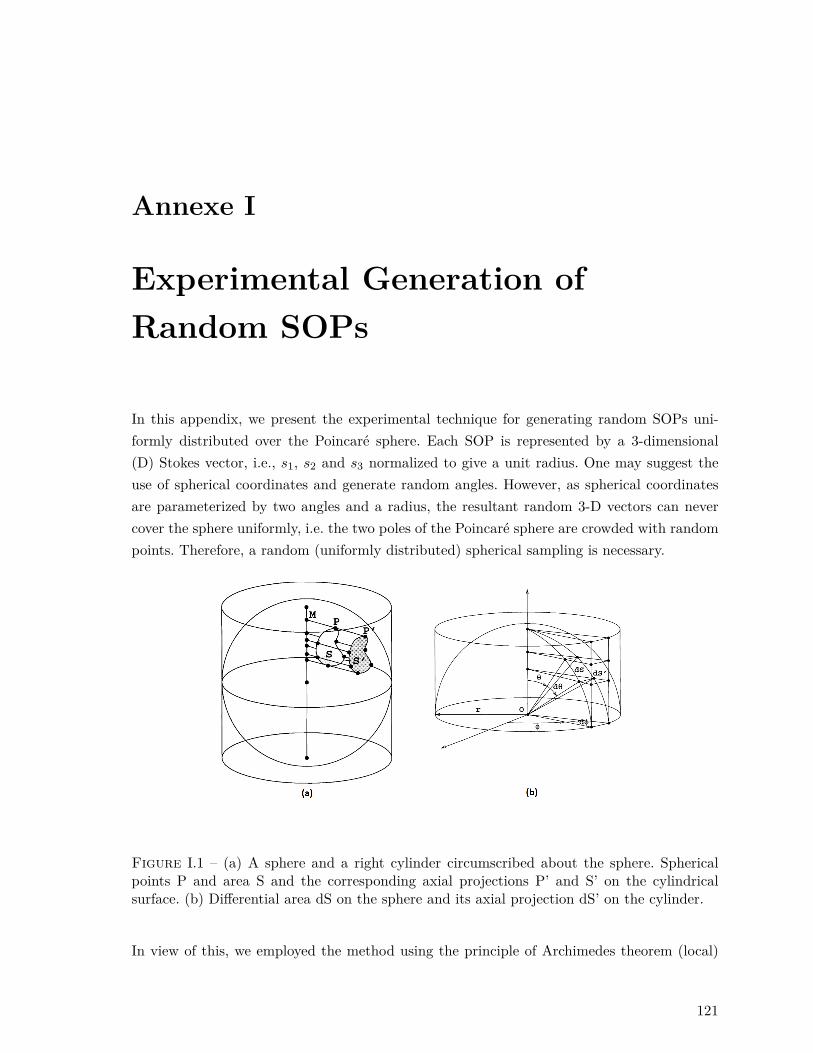
Annexe I

Experimental Generation ofRandom SOPs

In this appendix, we present the experimental technique for generating random SOPs uni-formly distributed over the Poincaré sphere. Each SOP is represented by a 3-dimensional(D) Stokes vector, i.e., s1, s2 and s3 normalized to give a unit radius. One may suggest theuse of spherical coordinates and generate random angles. However, as spherical coordinatesare parameterized by two angles and a radius, the resultant random 3-D vectors can nevercover the sphere uniformly, i.e. the two poles of the Poincaré sphere are crowded with randompoints. Therefore, a random (uniformly distributed) spherical sampling is necessary.

Figure I.1 – (a) A sphere and a right cylinder circumscribed about the sphere. Sphericalpoints P and area S and the corresponding axial projections P’ and S’ on the cylindricalsurface. (b) Differential area dS on the sphere and its axial projection dS’ on the cylinder.

In view of this, we employed the method using the principle of Archimedes theorem (local)

121

suggested by Shao and Badler [54] in 1996, where axial projection of any measurable regionon a sphere onto the right circular cylinder circumscribed about the sphere preserves area.

Refer to Fig. I.1a. Suppose P is a point on the sphere and M , a point on the axis of thecircumscribed cylinder, is the closest point to P . Extrapolate the line MP to intersect thesurface of the cylinder at point P ′. The point P ′ is called the axial projection of the point Pon a spherical surface onto the surface of the right circular cylinder circumscribed about thesphere. The above theorem means that the area S′ is equal to the area S. Mathematically,one has to prove that the two differential areas, dS and dS′ are equal to each other shown inFig. I.1b. For details, please refer to [54].

As random sampling (with uniform distribution) can be easily done on a cylindrical surface,we can generate a random point on the cylinder [-1, 1]×[0, 2π], and then find its inverseaxial projection on the Poincaré sphere. For random sampling on a surface, please refer toLeon-Garcia’s textbook [14]. As a result, the random spherical sampling avoids the crowdedrandom points on the two poles of the Poincaré sphere.

In experiment, we could only control five waveplates (4 quarter waveplates with a half wave-plates at the middle) but not the 3-D Stokes parameters inside the polarization synthesizer(Agilent N7786B), and a calibration (mapping between waveplates’ positions and 3-D Stokesparameters ) was necessary. Since the N7786B is not able to measure the Stokes parametersof DP-QPSK signals (which behaves as if a unpolarized light due to random data), only acontinuous wave without modulation was used for calibration. We adjusted only 3 waveplatesin N7786B to cover the Poincaré sphere as densely as possible, and recorded the correspondingStokes parameters in a look-up table. Thus, the randomly generated stokes parameters canbe used to sweep SOPs using the N7786 via our own look-up table.

Figure I.2 – The results of random spherical sampling showing (a) 1000 random SOPs ; (b)500 random SOPs (interleaved from (a) ) ; (c) 250 random SOPs (interleaved from (a) ).

122

Annexe J

Publication List

The followings are my publications since 2010.

1. W. C. Ng, A. T. Nguyen, C. S. Park, and L. A. Rusch, “Enhancing Clock Tone via Po-larization Pre-rotation : A Low-complexity, Extended Kalman Filter-based Approach,”submitted to Optical Fiber Communication Conference, March, 2015.

2. W. C. Ng, A. T. Nguyen, C. S. Park, and L. A. Rusch, “MIMO-FIR Tap Reduction viaPolarization Pre-rotation for 100 Gbps Short-Reach Applications,” submitted to IEEEJ. Lightw. Technol.

3. W. C. Ng, A. T. Nguyen, C. S. Park, and L. A. Rusch, “Reduction of MIMO-FIR Tapsvia SOP-Estimation in Stokes Space for 100 Gbps Short Reach Applications,” EuropeanConference and Exhibition on Optical Communication, September, 2014, P3.3.

4. A. T. Nguyen,W. C. Ng, C. S. Park, and L. A. Rusch, “An optimized 16-QAM constel-lation for mitigating impairments of phase noise and limited transmitter ENOB inoptical coherent detection systems,” European Conference and Exhibition on OpticalCommunication, September, 2014, Tu.1.3.5.

5. W. C. Ng, A. T. Nguyen, S. Ayotte, C. S. Park, and L. A. Rusch, “Overcoming PhaseSensitivity in Real-time Parallel DSP for Optical Coherent Communications : OpticallyFiltered Lasers,” IEEE J. Lightw. Technol., Vol. 32, No. 3, pp. 411 - 420, Feb. 2014.http://ieeexplore.ieee.org/xpl/articleDetails.jsp?tp=&arnumber=6678710

6. W. C. Ng, A. T. Nguyen, S. Ayotte, C. S. Park, and L. A. Rusch, “Impact of SinusoidalTones on Parallel Decision-Directed Phase Recovery for 64-QAM,” IEEE PhotonicsLetters Technology, Vol. 26, No. 5, pp. 486 - 489, Mar. 2014. http://ieeexplore.

ieee.org/xpl/articleDetails.jsp?tp=&arnumber=6701345

7. T. N. Huynh, A. T. Nguyen, W. C. Ng, L. Nguyen, L. A. Rusch, and L. P. Barry,“BER Performance of Coherent Optical Communications Systems Employing Monoli-thic Tunable Lasers With Excess Phase Noise,” IEEE J. Lightw. Technol., Vol. 32, No.10, pp. 1973 - 1980 May. 2014.

123

8. W. C. Ng, A. T. Nguyen, S. Ayotte, C. S. Park, and L. A. Rusch, “Parallel and Pi-pelined Decision-Directed Phase Recovery for 64-QAM in the Presence of SinusoidalTones,” Optical Fiber Communication Conference, M2A.4, March, 2014.

9. B. Filion , W. C. Ng, An T. Nguyen, L. A. Rusch and S. LaRochelle, “Widebandwavelength conversion of 16 Gbaud 16-QAM and 5 Gbaud 64-QAM signals in a semi-conductor optical amplifier, ” Optics Express, Vol. 21, Issue 17, pp. 19825-19833 ,2013.

10. B. Filion ,W. C. Ng, An T. Nguyen, L. A. Rusch and S. LaRochelle, “Wideband Wave-length Conversion of 5 Gbaud 64-QAM Signals in a Semiconductor Optical Amplifier,”European Conference and Exhibition on Optical Communication, P.3.19, September,2013.

11. W. C. Ng, T. N. Huynh, A. T. Nguyen, S. Ayotte, C. S. Park, L. P. Barry and L.A. Rusch, “Improvement due to Optically Filtered Lasers in Parallel Decision-DirectedPhase Recovery for 16-QAM,” The 10th Conference on Lasers and Electro-Optics PacificRim, and The 18th OptoElectronics and communications Conference / Photonics inSwitching 2013, WR3-2, June 2013.

12. T. Huynh, W. C. Ng, A. T. Nguyen, L. Nguyen, L. Rusch, and L.Barry, “TrackingExcess Noise from a Monolithic Tunable Laser in Coherent Communication Systems,”Optical Fiber Communication Conference 2013, JW2A.46, March, 2013.

13. W. C. Ng, A. T. Nguyen, S. Ayotte, C. S. Park, L. A. Rusch, “Optically-filtered LaserSource Enabling Improved Phase Tracking in Coherent Transmission Systems,” Euro-pean Conference and Exhibition on Optical Communication, P.3.15, September, 2012.

14. K. Dolgaleva, W. C. Ng, , L. Qian, J. S. Aitchison, M. Carla Camasta and Mark Sorel,“Compact Highly-Nonlinear AlGaAs Waveguides for Efficient Wavelength Conversion,” Optics Express, Vol. 19, pp. 12440-12455, 2011.

15. W. C. Ng, Q. Xu, K. Dolgaleva, S. Doucet, D. Lemus, P. Chretien, W. Zhu, L. A.Rusch, S. LaRochelle, L. Qian, J. S. Aitchison, “Error-free 0.16pi-XPM-based All-Optical Wavelength Conversion in a 1-cm-long AlGaAs waveguide, ” Proc. IEEE Pho-tonics Society Annual Meeting 2010, pp. 54-55 , November, 2010.

16. K. Dolgaleva, W. C. Ng, L. Qian, and J. S. Aitchison, “Efficient Self-Phase Modula-tion, Cross-Phase Modulation, and Four-Wave Mixing in AlGaAsWaveguides, ” Frontierin Optics 2010, FTuC5, October, 2010.

17. K. Dolgaleva,W. C. Ng, L. Qian, J. S. Aitchison ,M. C. Camasta and M. Sorel, “Broad-band Self-Phase Modulation, Cross-Phase Modulation, and Four-Wave Mixing in 9-mm-long AlGaAs Waveguides, ” Optics Letters, Vol. 35, Issue 24, pp. 4093-4095, 2010.

18. A. D. Simard, N. Ayotte, Y. Painchaud, S. Bédard, and S. LaRochelle, “Impact ofSidewall Roughness on Integrated Bragg Gratings, ” IEEE J. Lightw. Technol., Vol. 29,No. 24, pp. 3693 - 3704, Dec. 2011. (Personal tutoring 1 to A. D. Simard.)

1. Contributions on methodology and on derivation for equations (15) – (26), Appendix A and B

124

Bibliographie

[1] Govind P. Agrawal. Nonlinear Fiber Optics. Academic Press, Inc., 2001.

[2] S. Ayotte, F. Costin, G. Brochu, M. J. Picard, A. Babin, X. Liu F. Pelletier, andS.Chandrasekhar. White Noise Filtered C-band Tunable Laserfor Coherent TransmissionSystems. In Optical Fiber Communication Conference, page OTu1G5, 2012.

[3] X. Chen, A. A. Amin, and W. Shieh. Characterization and Monitoring of Laser Line-widths in Coherent Systems. IEEE Journal of Lightwave Technology, 29(17) :2533–2537,September 2011.

[4] D. Crivelli, M. Hueda, H. Carrer, and J. Zacha. A 40nm CMOS single-chip 50GbpsDPQPSK or BPSK transceiver with electronic dispersion compensation for coherent op-tical channels. In International Solid-State Circuits Conference, pages 328–330, Feburary2012.

[5] D. E. Crivelli, M. R. Hueda, H. S. Carrer, M. del Barcoand R. R. Lopez, P. Gianni,J. Finochietto, N. Swenson, P. Voois, and O. E. Agazzi. Architecture of a Single Chip50 Gbps DP QPSK BPSK Transceiver with Electronic Dispersion Compensation forCoherent Optical Channels. IEEE Transactions on Circuits and Systems 1, 61(4) :1012,March 2014.

[6] J.-M. Delgado-Mendinueta, B. J. Puttnam, R. S. Luis, S. Shinada, and N. Wada. FastEqualizer Kernel Initialization for Coherent PDM-QPSK Burst-mode Receivers Basedon Stokes Estimator. In Signal Processing in Photonic Communication, page SPM2E.2,Rio Grande, Puerto Rico United States, July 2013.

[7] D. Derickson. Fiber optics test and measurement. Prentice Hall PTR, 1998.

[8] I. Fatadin, D. Ives, and S. J. Savor. Laser linewidth tolerance for 16-QAM coherentoptical systems using QPSK partitioning. IEEE Photonics Technology Letters, 22 :631–633, May 2010.

[9] I. Fatadin, D. Ivex, and S. J. Savory. Blind Equalization and Carrier Phase Recovery in a16-QAMOptical Coherent System. IEEE Journal of Lightwave Technology, 27(15) :3042–2049, August 2009.

125

[10] B. Filion, W. C. Ng, A. T. Nguyen, L. A. Rusch, and S. LaRochelle. Wideband Wave-length Conversion of 5 Gbaud 64 QAM Signals in a Semiconductor Optical Amplifier. InEuropean Conference and Exhibition on Optical Communication, page P.3.19, London,September 2013.

[11] Wolfgang Freude, Rene Schmogrow, Philipp C. Schindler, Stefan Wolf, Bernd Nebendahl,Christian Koos, and Juerg Leuthold. Polarisation Demultiplexing in Coherent Receiverswith Real-Time Digital Signal Processing. In Transparent Optical Networks (ICTON),2013.

[12] H. Fu and P. Y. Kam. Exact phase noise model and its application to linear minimumvariance estimation of frequency and phase of a noisy sinusoid. In IEEE 19th Interna-tional Symposium on Personal, Indoor and Mobile Radio Communications, September2008.

[13] Y. Gao, A. P. T. Lau, C. Lu, J. Wu, Y. Li, X. Kun, W. Li, and T. J. Lin. Low-ComplexityTwo Stage Carrier Phase Estimation for 16 QAM Systems using QPSK Partitioningand Maximum Likelihood Detection. In Optical Fiber Communication Conference, pageOMJ6, 2011.

[14] Alberto Leon Garcia. Probability and Random Processes for Electrical Engineering. Pear-son Education, 2008.

[15] R. D. Gaudenzi, T. Garde, and V. Vanghi. Performance anaylsis of decision directedmaximum likelihood phase estimators for M PSK modulated signals. IEEE Transactionson Communication, 43(12) :3090–3100, December 1995.

[16] P. Gianni, G. Corral Briones, H. Carrer, and M. Hueda. Compensation of laser frequencyfluctuations and phase noise in 16-QAM coherent receivers. IEEE Photonics TechnologyLetters, 25(5) :442–445, March 2013.

[17] P. Gianni, G. Corral Briones, C. Rodriguez, H. Carrer, and M. Hueda. A new parallelcarrier recovery architecture for intradyne coherent optical receivers in the presence oflaser frequency fluctuations. In IEEE Global Telecommunications Conference, pages 1–6,December 2011.

[18] A. H. Gnauck, P. Winzer, A. Konczykowska, F. Jorge, J. Y. Dupuy, M. Riet, G. Charlet,B. Zhu, and D. W. Peckham. Generation and Transmission of 21.4 Gbaud PDM 64 QAMusing a High Power DAC Driving a Single I Q modulator. IEEE Journal of LightwaveTechnology, 30(4) :532–536, 2012.

[19] F. N. Hauske, N. Stojanovic, C. Xie, and M. Chen. Impact of Optical Channel Distortionto Digital Timing Recovery in Digital Coherent Transmission Systems. In InternationalConference on Transparent Optical Networks, page We.D1.4, 2010.

126

[20] F. N. Hauske, C. Xie, N. Stojanovic, and M. Chen. Analysis of Polarization Effects toDigital Timing Recovery in Coherent Receivers of Optical Communication Systems. InPhotonische Netze, page P6, 2010.

[21] Keang Po Ho. Phase modulated optical communication systems. Springer, 2005.

[22] L. Huang, D. Wang, A. P. T. Lau, C. Lu, , and S. He. Performance analysis of blindtiming phase estimators for digital coherent receivers. Optics Express, 22(6) :6749–6763,March 2014.

[23] E. Ip and J. Kahn. Feedforward Carrier Recovery for Coherent Optical Communications.Journal of Lightwave Technology, 25(9) :2675–2692, September 2007.

[24] Steven M. Kay. Fundamentals of Statistical Signal Processing Estimation Theory. Pren-tice Gall Signal Processing Series. Pearson, 1993.

[25] K. Kikuchi. Characterization of semiconductor-laser phase noise and estimation of bit-error rate performance with low-speed offline digital coherent receivers. Optics Express,20(5) :5291–2302, Feb 2011.

[26] K. Kikuchi. Clock Recovering Characteristics of Adaptive Finite Impulse Response filtersin Digital Coherent Optical Receivers. Optics Express, 19(6) :5611–5619, March 2011.

[27] K. Kikuchi. Performance Anaylsis of Polarization Demultiplexing based on Constant-Modulus Algorithm in Digital Coherent Receiver. Optics Express, 19(10) :9868, 2011.

[28] H. Kogelnik and P. Winzer. PMD Outage Probabilities Revisited. In Optical FiberCommunication Conference, page OTuN3, 2007.

[29] M. Kuschnerov, T. Bex, and P. Kainzmaier. Energy efficient Digital Signal Processing.In Optical Fiber Communications Conference, page Th3E.7, San Francisco, CA, USA,2014.

[30] M. Kuschnerov, K. Piyawanno, M. Alfiad, B. Spinnler, A. Napoli, and B. Lankl. Impact ofmechanical vibrations on laser stability and carrier phase estimation in coherent receivers.IEEE Photonics Technology Letters, 22(15) :1114–1116, August 2010.

[31] M. Kuschnerov, K. Piyawanno, M.S. Alfiad, B. Spinnler, A. Napoli, and B. Lankl. DGD-tolerant Timing Recovery for Coherent Receivers. In OptoElectronics and Communica-tions Conference, pages 7B1–4, Sopporo Convention Center, Japan, July 2010.

[32] A. P. T. Lau, T. S. R. Shen, W. Shieh, and K.-P. Ho. Equalization enhanced phasenoise for 100Gbps transmission and beyond with coherent detection. Optics Express,18(16) :17239–17251, 2010.

127

[33] D. Lavery, R. Maher, D. Millar, B. C. Thomsen, P. Bayvel, and S. Savory. Demonstrationof 10 Gbit/s colorless coherent PON incorporating tunable DS-DBR lasers and low-complexity parallel DSP. In Optical Fiber Communication Conference, page PDP5B.10,Los Angeles, California United States, March 2012.

[34] D. B. Leeson. A simple model of feedback oscillator noise spectrum. In IEEE, volume 54,pages 329–330, February 1966.

[35] M. Li, N. Deng, F. N. Hauske, Q. Xue, X. Shi, Z. Feng, S. Cao, and Q. Xiong. OpticalBurst-mode Coherent Receiver with a Fast Tunable LO for Receiving Multi-wavelengthBurst Signals. In Optical Fiber Communication Conference, page OTu1G, 2012.

[36] N. C. Mantzoukis, C. S. Petrou, A. Vgenis, T. Kamalakis, I. Roudas, and L. Raptis. Ou-tage Probability due to PMD in Coherent PDM QPSK Systems with Electronic Equali-zer. IEEE Photonics Technology Letters, 22(16) :1247–1249, August 2010.

[37] C. J. McKinstrie, H. Kogelnik, R. M. Jopson, S. Radic, and A. V. Kanaev. Four wavemixing in fibers with random birefringence. Optics Express, 12(10) :2033–2055, 2004.

[38] N. J. Muga and A. N. Pinto. Adaptive 3D Stokes Space Based Polarization Demulti-plexing Algorithm. IEEE Journal of Lightwave Technology, 32(19) :3290–3298, 2014.

[39] W. C. Ng, T. N. Huynh, A. T. Nguyen, S. Ayotte, C. S. Park, L. P. Barry, and L. A.Rusch. Improvement due to Optically Filtered Lasers in Parallel Decision-Directed PhaseRecovery for 16-QAM. In The 10th Conference on Lasers and Electro-Optics Pacific Rim,and The 18th OptoElectronics and communications Conference / Photonics in Switching2013, page P3.15, June 2013.

[40] W. C. Ng, A. T. Nguyen, S. Ayotte, C. S. Park, and L. A. Rusch. Optically-filteredLaser Source Enabling Improved Phase Tracking in Coherent Transmission Systems. InEuropean Conference and Exhibition on Optical Communication, page P3.15, September2012.

[41] M. Oerder and H. Meyr. Digital Filter and Square Timing Recovery. IEEE Transactionson Communications, 36(5) :605 – 612, May 1988.

[42] Keshab K. Parhi. VLSI Digital Signal Processing Systems : Design and Implementation.ISBN : 978-0-471-24186-7. Wiley, December 1998.

[43] W.-R. Peng, T. Tsuritani, and I. Morita. Transmission of highbaud PDM 64QAM signals.IEEE Journal of Lightwave Technology, 31(13) :2146–2162, July 2013.

[44] T. Pfau, S. Hoffmann, and R. N. Hardware-Efficient Coherent Digital Receiver ConceptWith Feedforward Carrier Recovery for M-QAM Constellations. IEEE Journal of Light-wave Technology, 27(8) :989–999, 2009 2009.

128

[45] F. Pittala, A. Mezghani, I. Slim, and J. A. Nossek. Low-complexity training-aided 2 by2 MIMO frequency domain fractionally-spaced equalization. Optical Fiber Communica-tions Conference, page Th2A.42, March 2014.

[46] F. Pittala, I. Slim, A. Mezghani, and J. A. Nossek. Training-Aided Frequency-DomainChannel Estimation and Equalization for Single-Carrier Coherent Optical TransmissionSystems. Journal of Lightwave Technology, 32(24) :4247–4261, December 2014.

[47] Vincent Poor. An Introduction of Signal Detection and Estimation. Springer, 1989.

[48] J. G. Proakis and D. G. Manolakis. Digital signal processing : principles, algorithms,and applications. Prentice Hall, 1996.

[49] M. Qiu, Q. Zhuge, X. Xu, M. Chagnon, M. Morsy Osman, and D. V. Plant. Simple andefficient frequency offset tracking and carrier phase recovery algorithms in single carriertransmission systems. Optics Express, 21(7) :8157–8165, April 2013.

[50] S. Savory. Digital Filters for coherent optical receivers. Optics Express, 16(2) :804, 2008.

[51] R. Schmogrow, P.C. Schindler, C. Koos, W. Freude, and J. Leuthold. Blind Polariza-tion Demultiplexing With Low Computational Complexity. IEEE Photonics TechnologyLetters, 25(13) :1230–1233, January 2013.

[52] M. Seimetz. Laser linewidth limitations for optical systems with highorder modulationemploying feed forward digital carrier phase estimation. In Optical Fiber CommunicationConference, page OTuM2, March 2008.

[53] M. Selmi, Y. Jaouen, and P. Cibalt. Accurate digital frequency offset estimator forcoherent PolMux QAM transmission systems. In European Conference and Exhibitionon Optical Communication, page P3.08, Vienna, Austria, September 2009.

[54] M.-Z. Shao and N. Badler. Spherical sampling by Archimedes’ theorem. Technical ReportMS-CIS-96-02, University of Pennsylvania, Department of Computer and InformationScience, 1996.

[55] K. Shi, R. Watts, D. Reid, T.N. Huynh, C. Browning, P.M. Anadarajah, F. Smyth, andL. P. Barry. Dynamic Linewidth Measurement Method via an Optical Quadrature FrontEnd. IEEE Photonics Technology Letters, 23(21) :1591 – 1593, 2011.

[56] W. Shieh and K.-P. Ho. Equalization enhanced phase noise for coherent detection systemsusing electronic digital signal processing. Optics Express, 16(20) :15718–15727, 2008.

[57] R. A. Soriano, F. N. Hauske, N. G. Gonzalez, Z. Zhang, Y. Ye, and I. T.Monroy. Chro-matic Dispersion Estimation in Digital Coherent Receivers. IEEE Journal of LightwaveTechnology, 29(11) :1627 –1637, June 2011.

129

[58] J. Stanley. High-Speed ASIC for Optical Communications. In Optical Fiber Communi-cations Conference, page Th3E.7, San Francisco, CA, USA, 2014.

[59] N. Stojanovi, B. Mao, and Y. Zhao. Digtial phase detector for nyquist and faster thannyquist systems. IEEE Communications Letters, 18(3) :511–514, March 2014.

[60] N. Stojanovi, Y. Zhao, and C. Xie. Feed-Forward and Feedback Timing Recovery forNyquist and Fast than Nyquist Systems. In Optical Fiber Communication Conference,page Th3E.3, 2014.

[61] N. Stojanovic, C. Xie, Y. Zhao, B. Mao, and N. G. Gonzalez. A circuit enabling clockextraction in coherent receivers. In European Conference and Exhibition on OpticalCommunication, page P3.08, 2012.

[62] H. Sun and K.-T. Wu. A novel dispersion and PMD tolerant clock phase detector forcoherent transmission. In Optical Fiber Communication Conference, page OMJ4, LosAngeles, CA, USA, 2011.

[63] B. Szafraniec, T. S. Marshall, and B. Nebendahl. Performance Monitoring and Mea-surement Techniques for Coherent Optical Systems. Journal of Lightwave Technology,31(4) :648– 663„ February 2013.

[64] B. Szafraniec, B. Nebendahl, and T. Marshall. Polarization Demultiplexing in StokesSpace. Optics Express, 18(17) :17928–17939, August 2010.

[65] M. G. Taylor. Phase Estimation Methods for Optical Coherent Detection Using DigitalSignal Processing. Journal of Lightwave Technology, 27(7) :901–914, 2009.

[66] F. Vacondio, C. Simonneau, A. Voicila, E. Dutisseuil, J.-M. Tanguy, J.-C. Antona,G. Charlet, and S. Bigo. Real time implementation of packet-by-packet polarizationdemultiplexing in a 28 Gb/s burst mode coherent receiver. In Optical Fiber Communi-cation Conference, page OM3H.6, Los Angeles, California United States, March 2012.

[67] H. E. Weste and D. M. Harris. CMOS VLSI design : a circuts and systems perspective.Pearson Education, Inc., Addison Wesley, 2011.

[68] P. J. Winzer and G. J. Foschini. Mode Division Multiplexed Transmission System. InOptical Fiber Communication Conference, page Th1J.1, 2014.

[69] P. J. Winzer, A. H. Gnauck, C. R. Doerr, M. Magarini, and L. L. Buhl. Spectrallyefficient long-haul optical networking using 112 Gbps polarization multiplexed 16 QAM.IEEE Journal of Lightwave Technology, 28(4) :547–556, Feb 2010.

[70] P. J. Winzer, A. H. Gnauck, A. Konczykowska, F. Jorge, and J. Y. Dupuy. Penalties fromIn Band Crosstalk for Advanced Optical Modulation Formats. In European Conferenceand Exhibition on Optical Communication, page Tu.5.B, 2011.

130

[71] K.-T. Wu and H. Sun. Frequency-Domain Clock Phase Detector for Nyquist WDMSystems. In Optical Fiber Communications Conference, page Th3E.2, San Francisco,CA, USA„ 2014.

[72] C. Xie and S. Chandrasekhar. Two-stage constant modulus algorithm equalizer for sin-gularity free operation and optical performance monitoring in optical coherent receiver.Optical Fiber Communication Conference, page OMK3, March 2010.

[73] Z. Yu, X. Yi, Q. Yang, M. Luo, J. Zhang, L. Chen, and K. Qiu. Experimental Demons-tration of Polarization Demultiplexing in Stokes Space for Coherent Optical OFDM. InOptical Fiber Communication Conference, page OW3B, March 2013.

[74] Z. Yu, X. Yi, J. Zhang, M. Deng, H. Zhang, and K. Qiu. Modified Constant Moduolus al-gorithm with Polarization Demultiplexing in Stokes Space in Optical Coherent Receiver.IEEE Journal of Lightwave Technology, 31(19) :3203 – 3209, 2013.

[75] S. Zhang, C. Yu, P. Y. Kam, and J. Chen. Parallel Implementation of Decision-AidedMaximum-Likelihood Phase Estimation in Coherent M-ary Phase-Shift Keying Systems.IEEE Photonics Technology Letters, 21(19) :1363–1365, October 2009.

[76] X. Zhou, L. E. Nelson, P. Magill, R. Isaac, B. Zhu, D. W. Peckham, P. I. Borel, andK. Carlson. High Spectral Efficiency 400 Gbps Transmission Using PDM Time DomainHybrid 32/64 QAM and Training Assisted Carrier Recovery. IEEE Journal of LightwaveTechnology, 31(7) :999–1005, April 2013.

[77] Q. Zhuge, M. E. Pasandi, X. Xu, B. Chatelain, Z. Pan, and M. Osman. Linewidthtolerant low complexity pilot aided carrier phase recovery for M QAM using superscalarparallelization. In Optical Fiber Communication Conference, page OTu2G.2, Los Angeles,CA, USA, 2012.

131