Digital Resonators “Discrete-Time Oscillator Theory” Clay S. Turner

Welcome message from author
This document is posted to help you gain knowledge. Please leave a comment to let me know what you think about it! Share it to your friends and learn new things together.
Transcript

Digital Resonators
“Discrete-Time Oscillator Theory” Clay S. Turner
(c) 2010 Clay S. Turner
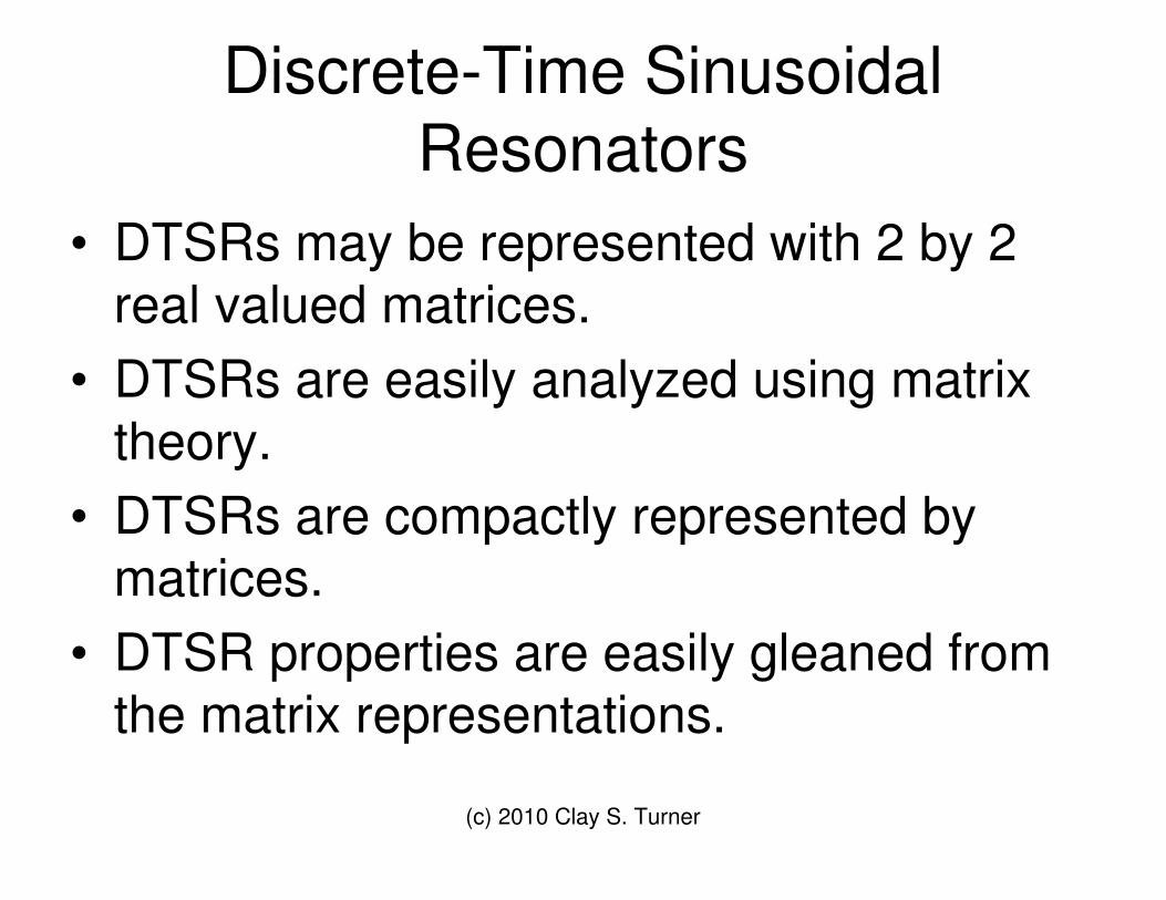
Discrete-Time Sinusoidal Resonators
• DTSRs may be represented with 2 by 2 real valued matrices.
• DTSRs are easily analyzed using matrix theory.
• DTSRs are compactly represented by matrices.
• DTSR properties are easily gleaned from the matrix representations.

(c) 2010 Clay S. Turner
Trigonometric Recursion
• Early example from Francois Vieta (1572). Vieta used this formula to recursively generate trig tables.
)cos()cos()cos(2)cos( qpqpqp −−⋅=+
(c) 2010 Clay S. Turner
Trigonometric Recursion
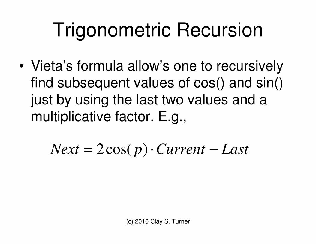
• Vieta’s formula allow’s one to recursively find subsequent values of cos() and sin() just by using the last two values and a multiplicative factor. E.g.,
LastCurrentpNext −⋅= )cos(2
(c) 2010 Clay S. Turner
Network to Matrix Formulation
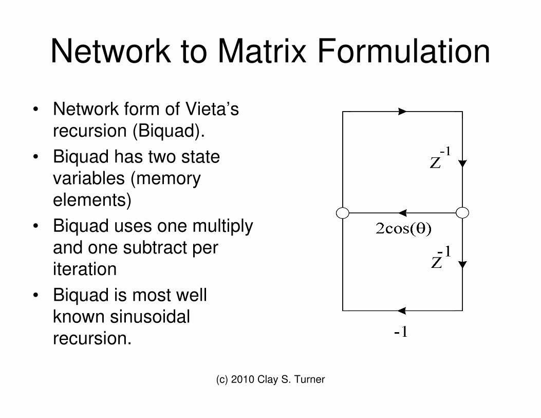
• Network form of Vieta’s recursion (Biquad).
• Biquad has two state variables (memory elements)
• Biquad uses one multiply and one subtract per iteration
• Biquad is most well known sinusoidal recursion.

(c) 2010 Clay S. Turner
Network to Matrix Formulation
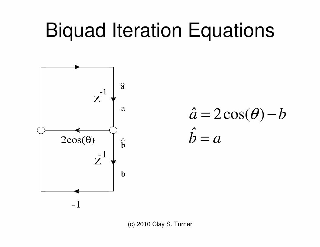
• Label inputs and the outputs of each memory element in the network.
• Then write each input’s equation in terms of all outputs.
(c) 2010 Clay S. Turner
Biquad Iteration Equations
ab
ba
=−=
ˆ)cos(2ˆ θ
(c) 2010 Clay S. Turner
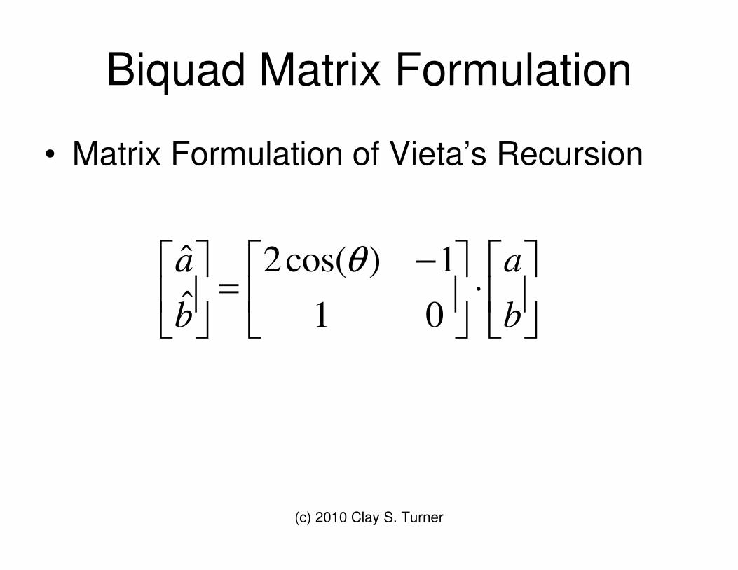
Biquad Matrix Formulation
• Matrix Formulation of Vieta’s Recursion
��
���
�⋅��
���
� −=�
�
���
�
b
a
b
a
011)cos(2
ˆˆ θ

(c) 2010 Clay S. Turner
Another Trigonometric Example
• Example with two coupled equations
)sin()cos()cos()sin()sin()sin()sin()cos()cos()cos(
qpqpqp
qpqpqp
⋅+⋅=+⋅−⋅=+
(c) 2010 Clay S. Turner
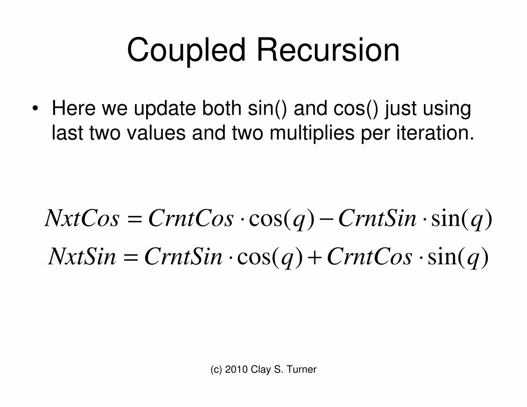
Coupled Recursion
• Here we update both sin() and cos() just using last two values and two multiplies per iteration.
)sin()cos()sin()cos(
qCrntCosqCrntSinNxtSin
qCrntSinqCrntCosNxtCos
⋅+⋅=⋅−⋅=

(c) 2010 Clay S. Turner
Coupled Iteration Equations
• Just like with the biquad structure, we may write the iteration equations in a similar manner.
• The step angle per iteration is
)sin()cos(ˆ)sin()cos(ˆ
θθθθ
⋅+⋅=⋅−⋅=
abb
baa
θ
(c) 2010 Clay S. Turner
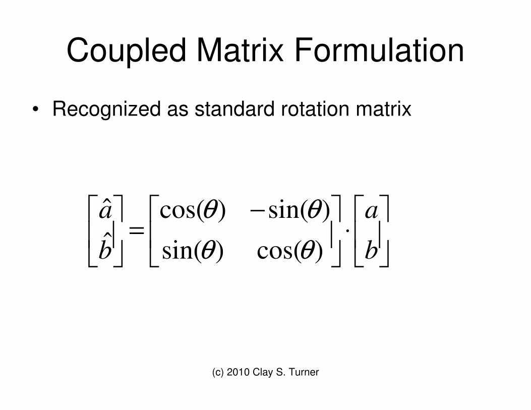
Coupled Matrix Formulation
• Recognized as standard rotation matrix
��
���
�⋅��
���
� −=�
�
���
�
b
a
b
a
)cos()sin()sin()cos(
ˆˆ
θθθθ

(c) 2010 Clay S. Turner
Discrete-Time Oscillator Structure
• The two example oscillators have the following in common:
• Each uses 2 state variables. • The matrix in each case is 2 by 2.

(c) 2010 Clay S. Turner
Discrete-Time Linear Oscillators
• So we will look at the following types of oscillator iterations (based on a general 2 by 2 matrix) more closely:
��
���
�⋅��
���
�=�
�
���
�
b
a
b
a
2221
1211
ˆˆ
αααα

(c) 2010 Clay S. Turner
Discrete-Time Barkhausen Criteria
• From the point of view of repeated iteration we see the nth output of the oscillator is simply:
02221
1211
ˆˆ
��
���
�⋅�
�
���
�=�
�
���
�
b
a
b
an
nαααα

(c) 2010 Clay S. Turner
Resonator Theory
• Besides looking at known trigonometric relations, how do we find new oscillator structures?
• Answer: We develop our own theory with guidance from analog theory.

(c) 2010 Clay S. Turner
Barkhausen’s Linear Oscillator Theory
• Heinrich Barkhausen modeled a linear oscillator as a linear amplifier with its output fed back in to its input and then stated two necessary criteria for oscillation.

(c) 2010 Clay S. Turner
Barkhausen Criteria
1. The amplifier gain times the feed back gain needs to equal unity.
2. The round trip delay needs to be a integral multiple of the oscillation period.

(c) 2010 Clay S. Turner
Discrete Time Osc. Theory
• So combining the matrix representation idea from our two examples with Barkhausen’s oscillator theory, we can come up with the discrete time counterparts to the Barkhausen Criteria.

(c) 2010 Clay S. Turner
Discrete Time Barkhausen Criteria
• The determinant of the oscillator matrix must be unity.
• The oscillator matrix when raised to some real power will be the identity matrix.
(c) 2010 Clay S. Turner
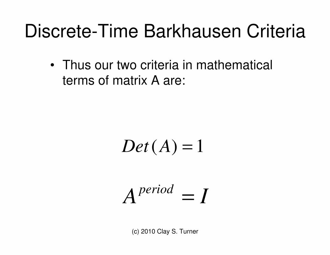
Discrete-Time Barkhausen Criteria
• Thus our two criteria in mathematical terms of matrix A are:
1)( =ADet
IAperiod =
(c) 2010 Clay S. Turner
Barkhausen’s 1st Criterion
• If we think of the two state variables as components of a vector, then Barkhausen’s 1st Criterion relates to length preservation. I.e., this says the length of the vector is unchanged by rotation.

(c) 2010 Clay S. Turner
Barkhausen’s 2nd criterion
• The periodicity constraint in combination with the unity gain means the oscillator matrix has complex valued eigenvalues.
• This in turn means the matrix’s “trace” has a magnitude of less than 2.

(c) 2010 Clay S. Turner
Discrete-Time Barkhausen Criteria • Thus our two criteria may alternatively be stated in
terms of the actual matrix elements:
121122211 =− αααα
22211 <+αα
(c) 2010 Clay S. Turner
Eigen-Theory
• A big advantage of using a matrix representation of the oscillator structure, is we can apply Linear Algebra with its tools to analyze oscillators.
• Eigentheory actually allows us to factor the matrix into a triple product where the step angle and the relative phases are readily apparent.

(c) 2010 Clay S. Turner
Oscillator Eigenvalues
• The oscillator matrix will have two eigenvalues that reside on the unit circle, and they are complex conjugates of each other.
• The eigenvalues are found to be:
��
�
� +== −±
2cos 22111 ααθλ θ wheree j

(c) 2010 Clay S. Turner
Oscillator Step Angle
• The angle theta is the step angle per iteration of the oscillator.
• Thus the oscillator frequency is determined wholly by the trace (delta) of the matrix!
)cos(2 θ=∆

(c) 2010 Clay S. Turner
Analysis of the off Diagonal Matrix Elements
• A study of the eigen values along with Barkhausen’s criteria will show that the “off diagonal” matrix elements must obey the following:
02112 <αα

(c) 2010 Clay S. Turner
Properties of the off Diagonal Matrix Elements
• Thus we see that neither off diagonal element may be zero!
• No oscillator matrix may be triangular. • And we see that they must have opposite
signs!
(c) 2010 Clay S. Turner
State Variables
• If the state variables are plotted as a function of time, they will each be a sinusoid, both with the same frequency, be out of phase and may have a relative amplitude not equal to one.

(c) 2010 Clay S. Turner
Relative Phase shift
• From a study of the eigenvectors, the relative phase shift between the state variables (b relative to a) is:
( )��
�
�
� +−+−=
12
222111122
24
argα
ααααφ
j

(c) 2010 Clay S. Turner
Relative Phase Shift (alternative)
• An alternative formulation for relative phase shift is:
( )1)sgn(22
cos 122112
11221 −+��
�
�
�
−−= − απ
ααααφ

(c) 2010 Clay S. Turner
Quadrature Criterion
• From the phase shift formula, we find that a relative phase of +-90 degrees requires the two elements making up the trace of the matrix to have the same value!
• Thus, from simply looking at an oscillator matrix we can ascertain if the oscillator is quadrature or not.
(c) 2010 Clay S. Turner
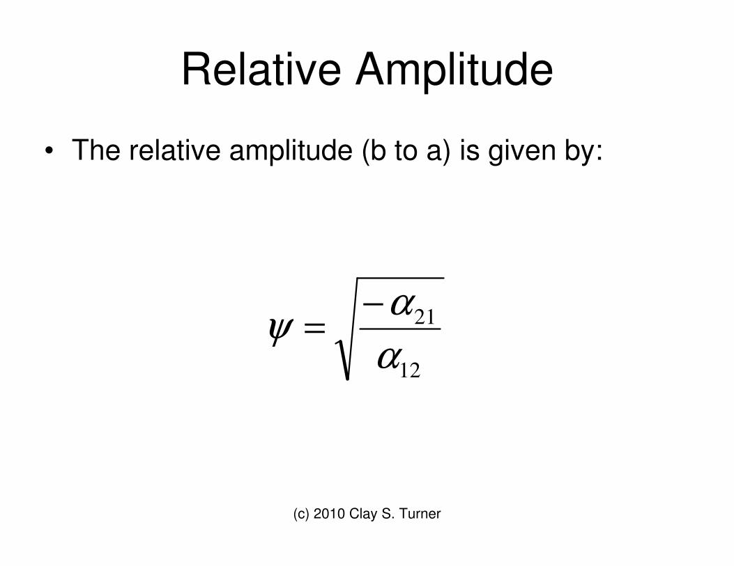
Relative Amplitude
• The relative amplitude (b to a) is given by:
12
21
ααψ −=
(c) 2010 Clay S. Turner
Relative Amplitude
• From our earlier work on the off diagonal elements, we know that the relative amplitude will always be a positive value.

(c) 2010 Clay S. Turner
Equi-Amplitude Criterion
• The relative amplitude relation tells us that if we are to have both state variables have the same amplitude, then we simply require:
2112 αα −=

(c) 2010 Clay S. Turner
Matrix Factoring
• The main point of the eigenanalysis is to factor the matrix. We find:
111
0011
−
−−− ��
���
�⋅��
���
�⋅��
���
�= φφθ
θ
φφ ψψψψ jjj
j
jj eee
eee
A

(c) 2010 Clay S. Turner
Matrix Exponentiation
• The factoring makes raising the matrix to a power straight forward and reveals the nature of theta.
111
0011
−
−−− ��
���
�⋅��
���
�⋅��
���
�= φφθ
θ
φφ ψψψψ jjjn
jn
jjn
eee
eee
A

(c) 2010 Clay S. Turner
Initialization
• Assuming we have a chosen oscillator matrix, then from eigen-theory, we find the state variables need to be initialized to
��
���
�=�
�
���
�
)cos(1
φψb
a
(c) 2010 Clay S. Turner
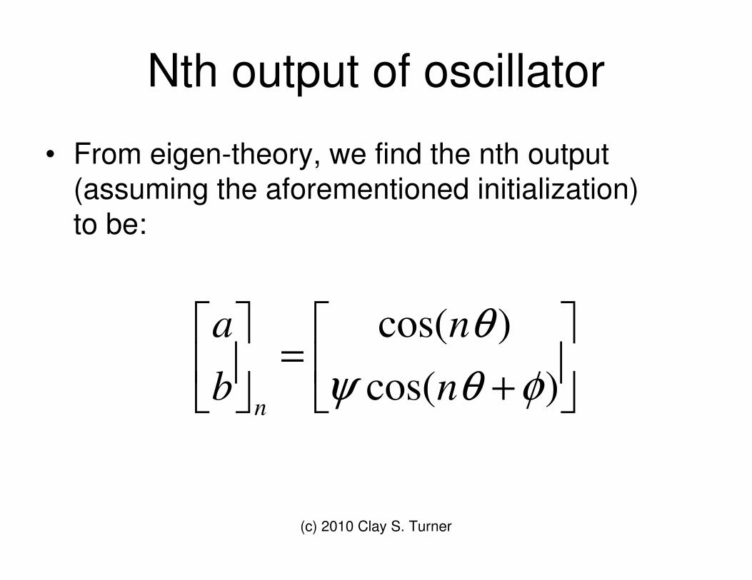
Nth output of oscillator
• From eigen-theory, we find the nth output (assuming the aforementioned initialization) to be:
��
���
�
+=�
�
���
�
)cos()cos(
φθψθ
n
n
b
a
n

(c) 2010 Clay S. Turner
Oscillator Amplitude
• The amplitude squared (energy) of the oscillator is given by:
)(sin
)cos(2
2
22
φψ
φψ
⋅⋅−���
�
�+=
baba
E
(c) 2010 Clay S. Turner
Amplitude Control
• To keep magnitude errors from growing, a simple “AGC” type of feedback may be employed. Thus a gain “G” is calculated every so often based on the energy, E, and is used to scale the state variables.
(c) 2010 Clay S. Turner
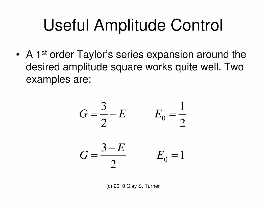
Useful Amplitude Control
• A 1st order Taylor’s series expansion around the desired amplitude square works quite well. Two examples are:
12
3
21
23
0
0
=−=
=−=
EE
G
EEG

(c) 2010 Clay S. Turner
Digital Waveguide Osc.
• Single Multiply, Quadrature Oscilator
��
���
�
+−
=kk
kkA
11

(c) 2010 Clay S. Turner
Dual Multiply - Quadrature
• This oscillator uses 2 multiplies per iteration, has quadrature outputs and uses staggered updating.
��
���
�
−−
=k
kkA
11 2
(c) 2010 Clay S. Turner
Staggered Updating
• The matrix formulation’s compactness is nice, but it implies a simultaneous updating of the state variables.
• Sequential updating may require temporary storage.
(c) 2010 Clay S. Turner
Staggered Updating
• Staggered updating is a method where one state variable is 1st updated and then that updated value is used in the 2nd update equation.
(c) 2010 Clay S. Turner
Staggered Update - Derivation
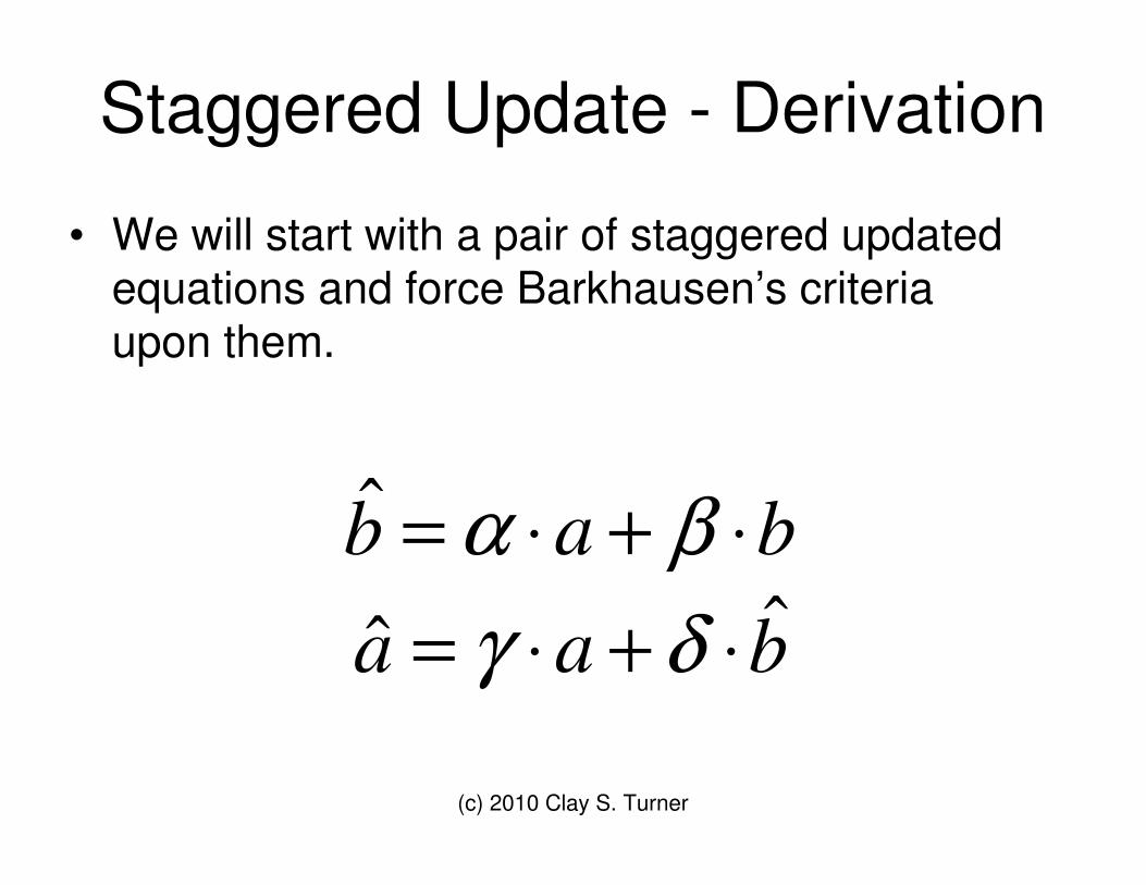
• We will start with a pair of staggered updated equations and force Barkhausen’s criteria upon them.
baa
babˆˆ
ˆ
⋅+⋅=⋅+⋅=
δγβα

(c) 2010 Clay S. Turner
Staggered Update - Derivation
• So now we insert the 1st update into the 2nd equation and we get the following matrix form:
��
���
� +=
βαβδαδγ
A
(c) 2010 Clay S. Turner
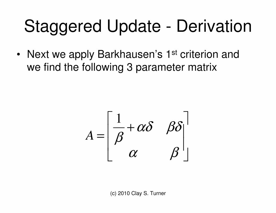
Staggered Update - Derivation • Next we apply Barkhausen’s 1st criterion and
we find the following 3 parameter matrix
��
�
�
��
�
� +=βα
βδαδβ1
A

(c) 2010 Clay S. Turner
EquiAmp-Staggered Update
• To be equi-amplitude, we just set the off-diagonal elements to be negatives of each other.
βδα −=

(c) 2010 Clay S. Turner
EquiAmp-Staggered Update
• Thus our 2 parameter equi-amplitude staggered update oscillator has the following form.
��
�
�
��
�
�
−
−=ββδ
βδβδβ
21A

(c) 2010 Clay S. Turner
EquiAmp-Staggered Update
• Now we can substitute some simple values for the parameters and get a couple of neat oscillators.
• First we will set:
1=β

(c) 2010 Clay S. Turner
Magic Circle Algorithm • The “magically” wonderful oscillator results:
��
���
�
−−
11 2
δδδ
(c) 2010 Clay S. Turner
Magic Circle Algorithm
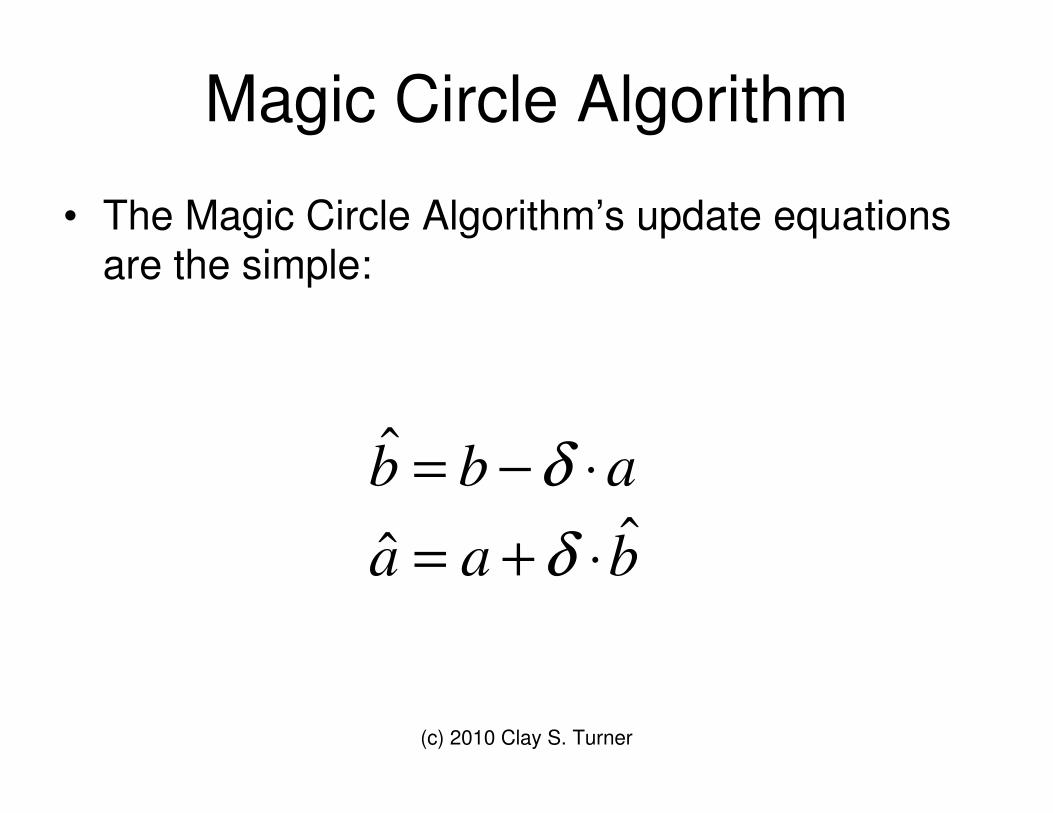
• The Magic Circle Algorithm’s update equations are the simple:
baa
abbˆˆ
ˆ
⋅+=⋅−=
δδ
(c) 2010 Clay S. Turner
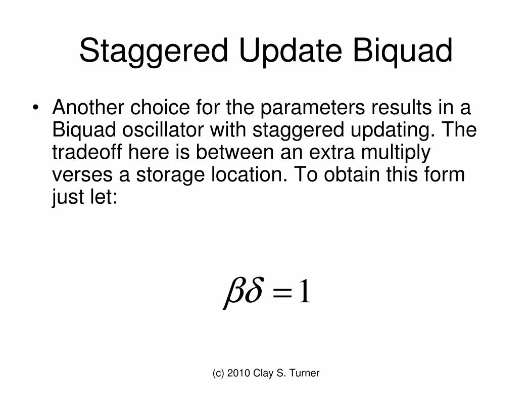
Staggered Update Biquad
• Another choice for the parameters results in a Biquad oscillator with staggered updating. The tradeoff here is between an extra multiply verses a storage location. To obtain this form just let:
1=βδ

(c) 2010 Clay S. Turner
Staggered Update Biquad
• The Staggered update biquad’s matrix form is:
��
���
�
−=
β110
A

(c) 2010 Clay S. Turner
Staggered Update Biquad
• The update equations are:
( )aba
abb
+⋅=
−⋅=ˆ1ˆ
ˆ
β
β

(c) 2010 Clay S. Turner
Reinsch (Staggered Update)
• If we relax the equiamplitude requirement and set 2 of the 3 parameters to unity, then we can obtain Reinsch’s formulation. For example:
11 == δβ
(c) 2010 Clay S. Turner
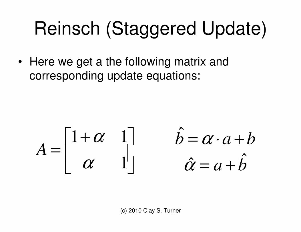
Reinsch (Staggered Update)
• Here we get a the following matrix and corresponding update equations:
ba
babA ˆˆ
ˆ
111
+=+⋅=
��
���
� +=
αα
αα

(c) 2010 Clay S. Turner
An Oscillator Application
• The venerable Goertzel Algorithm uses a Biquad oscillator for its calculation.
• However any oscillator may be used in the Goertzel Algorithm.
• Some oscillators will have better numerical properties than others. I.e., especially for low frequencies.
(c) 2010 Clay S. Turner
The Generalized Goertzel Algorithm
• Goertzel processes N values of data and computes a Fourier Coefficient (single frequency) for the data. We can describe this algorithm in four (five) main steps.

(c) 2010 Clay S. Turner
The Generalized Goertzel Algorithm (Step 1)
• Initialization – uses 1 datum.
��
���
�=
00
0
xy�

(c) 2010 Clay S. Turner
The Generalized Goertzel Algorithm (Step 2)
• Recursive computation with all input data. “A” is the oscillator matrix. For
��
���
�+⋅=−∈ − 0
},1,...,3,2,1{ 1i
ii
xyAyNi��

(c) 2010 Clay S. Turner
The Generalized Goertzel Algorithm (Step 3)
• Phase Compensation
1−⋅= NN yAy��
(c) 2010 Clay S. Turner
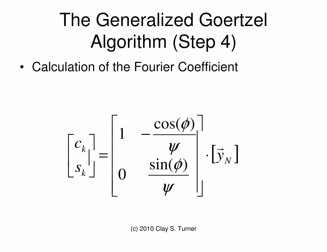
The Generalized Goertzel Algorithm (Step 4)
• Calculation of the Fourier Coefficient
[ ]Nk
k ys
c �⋅
����
�
�
����
�
� −=�
�
���
�
ψφ
ψφ
)sin(0
)cos(1

(c) 2010 Clay S. Turner
The Generalized Goertzel Algorithm (Step 5a)
• Energy Calculation assuming steps 3 and 4 are performed.
22kk scE +=

(c) 2010 Clay S. Turner
The Generalized Goertzel Algorithm (Step 5b)
• If the energy (amplitude squared) is all that is needed, then just skip steps 3 and 4 and calculate the following: (a and b) are the 2 elements of the last result from step 2.
ψφ
ψ)cos(
22
2 abb
aE −���
�
�+=

(c) 2010 Clay S. Turner
Improving Goertzel
• Some choices of oscillator design will yield better numerical accuracy than others.
• For comparison, we show the Biquad, Reinsch, and Magic Circle Oscillators and how they perform in Goertzel.
• For this test. N=1000 points

(c) 2010 Clay S. Turner
Extended Goertzel Results

(c) 2010 Clay S. Turner
Zoomed In View (Results)
(c) 2010 Clay S. Turner
Results Explaination
• In low frequency limit: • Biquad is in phase and equiamplitude • Reinsch is in phase and amplitudes are
unmatched • Magic Circle is quadrature and
equiamplitude.
(c) 2010 Clay S. Turner
Discrete Time Oscillators
• Thanks to all who are willing to listen ;-) • The End for Now!
Related Documents