Digital Mapping and Environmental …info.ornl.gov/sites/publications/files/Pub45517.pdfORNL/TM-2013/356 Digital Mapping and Environmental Characterization of the National Wild and

ORNL/TM-2013/356

Digital Mapping and Environmental Characterization of the National Wild and Scenic Rivers System

September 2013

Prepared by

Ryan A. McManamay, Ph.D. Peter Bonsall

DOCUMENT AVAILABILITY

Reports produced after January 1, 1996, are generally available free via US Department of Energy (DOE) SciTech Connect. Website http://www.osti.gov/scitech/ Reports produced before January 1, 1996, may be purchased by members of the public from the following source: National Technical Information Service 5285 Port Royal Road Springfield, VA 22161 Telephone 703-605-6000 (1-800-553-6847) TDD 703-487-4639 Fax 703-605-6900 E-mail [email protected] Website http://www.ntis.gov/support/ordernowabout.htm Reports are available to DOE employees, DOE contractors, Energy Technology Data Exchange representatives, and International Nuclear Information System representatives from the following source: Office of Scientific and Technical Information PO Box 62 Oak Ridge, TN 37831 Telephone 865-576-8401 Fax 865-576-5728 E-mail [email protected] Website http://www.osti.gov/contact.html

This report was prepared as an account of work sponsored by an agency of the United States Government. Neither the United States Government nor any agency thereof, nor any of their employees, makes any warranty, express or implied, or assumes any legal liability or responsibility for the accuracy, completeness, or usefulness of any information, apparatus, product, or process disclosed, or represents that its use would not infringe privately owned rights. Reference herein to any specific commercial product, process, or service by trade name, trademark, manufacturer, or otherwise, does not necessarily constitute or imply its endorsement, recommendation, or favoring by the United States Government or any agency thereof. The views and opinions of authors expressed herein do not necessarily state or reflect those of the United States Government or any agency thereof.

ORNL/TM-2013/356

Environmental Sciences Division

DIGITAL MAPPING AND ENVIRONMENTAL CHARACTERIZATION

OF NATIONAL WILD AND SCENIC RIVER SYSTEMS

Ryan A. McManamay*, Peter W. Bonsall1, Shelaine C. Hetrick, and Brennan T. Smith

Date Published: September 2013

Prepared by

OAK RIDGE NATIONAL LABORATORY

Oak Ridge, Tennessee 37831-6283

managed by

UT-BATTELLE, LLC

for the

U.S. DEPARTMENT OF ENERGY

under contract DE-AC05-00OR22725

*Corresponding Author: Ryan A. McManamay, Oak Ridge National Laboratory, 1 Bethel Valley Road, Bldg. 1505, Oak Ridge,

TN 37831-6038, Email: [email protected], Phone: 865-241-8668 1GeoCorps America, National Park Service, Washington, D.C.

iii

CONTENTS

Page

LIST OF FIGURES ...................................................................................................................................... v LIST OF TABLES ........................................................................................................................................ v LIST OF ACRONYMS ................................................................................................................................ v ABSTRACT ................................................................................................................................................ vii ACKNOWLEDGMENTS ........................................................................................................................... ix 1. INTRODUCTION ................................................................................................................................ 1

1.1 THE NEED TO ACCURATELY MAP NATIONAL WILD AND SCENIC RIVERS ............ 2 1.2 OBJECTIVES ............................................................................................................................. 4

2. MAPPING NATIONAL WILD AND SCENIC RIVERS ................................................................... 5 2.1 METHODS ................................................................................................................................. 5

2.1.1 Selection of a stream network framework ..................................................................... 5 2.1.2 Delineating the upstream and downstream boundaries of WSRs .................................. 5 2.1.3 Incorporating stream boundaries into NHD using the HEM tool .................................. 5 2.1.4 Comparison of new and old stream networks ................................................................ 5

2.2 RESULTS ................................................................................................................................... 6

3. CHARACTERIZING THE ENVIRONMENTAL CONTEXT OF WILD AND SCENIC

RIVERS .............................................................................................................................................. 11 3.1 METHODS ............................................................................................................................... 11 3.2 RESULTS ................................................................................................................................. 13

4. DISCUSSION ..................................................................................................................................... 19

5. REFERENCES ................................................................................................................................... 20

v

LIST OF FIGURES

Figure Page

Fig. 1. WSRs falling under full or partial National Park Service jurisdiction and that of other

agencies. .................................................................................................................................... 1 Fig. 2. Aerial views comparing NHD digitized version and USGS Hydrography (old version) for

coarse and fine representations of the (A and C, respectively) Lumber Wild and Scenic

River, North Carolina, and (B and D, respectively) Eel Wild and Scenic River

California. .................................................................................................................................. 7 Fig. 3. Aerial view depicting WSR-NHD and WSR-HYD versions of the Charley WSR in Alaska. .......... 8 Fig. 4. Depiction of database spatially connecting WSRs to ORNL NHAAP environmental data. ........... 12 Fig. 5. Eel WSR and adjacent protected lands owned by various agencies falling within a 500 m

buffer. ...................................................................................................................................... 16

LIST OF TABLES

Table Page

Table 1. Comparison of river mileage (US miles) for WSRs digitized according to NHD reaches

(WSR-NHD) and USGS Hydrography reaches (WSR-HYD) .................................................. 9 Table 2. Summary of protected lands and primary (majority), second, and third largest land-owning

entity within a 500 m buffered acreage around each WSR ..................................................... 14 Table 3. Summary of a sample of queries produced using National Wild and Scenic River ORNL-

NHAAP environmental attribution database ........................................................................... 17

ABBREVIATIONS, ACRONYMS, AND INITIALISMS

BLM Bureau of Land Management

EA Environmental Attribution

FWS US Fish and Wildlife Service

GIS Geospatial Information System

HEM Hydrography Event Management Tool

NHAAP National Hydropower Asset Assessment Program

NHD National Hydrography Dataset

NPS National Park Service

NWSRS National Wild and Scenic Rivers System

ORNL Oak Ridge National Laboratory

PLSS Public Land Survey System

USFS US Forest Service

USGS US Geological Survey

WSR Wild and Scenic River

WSRA Wild and Scenic River Act

WSR-HYD WSRs digitized using USGS hydrography (1:2M scale).

WSR-NHD WSRs digitized at the NHD high resolution (1:24k scale)

vii

ABSTRACT

Spatially accurate geospatial information is required to support decision-making regarding sustainable

future hydropower development. Under a memorandum of understanding among several federal agencies,

a pilot study was conducted to map a subset of National Wild and Scenic Rivers (WSRs) at a higher

resolution and provide a consistent methodology for mapping WSRs across the United States and across

agency jurisdictions. A subset of rivers (segments falling under the jurisdiction of the National Park

Service) were mapped at a high resolution using the National Hydrography Dataset (NHD). The spatial

extent and representation of river segments mapped at NHD scale were compared with the prevailing

geospatial coverage mapped at a coarser scale. Accurately digitized river segments were linked to

environmental attribution datasets housed within the Oak Ridge National Laboratory’s National

Hydropower Asset Assessment Program database to characterize the environmental context of WSR

segments. The results suggest that both the spatial scale of hydrography datasets and the adherence to

written policy descriptions are critical to accurately mapping WSRs. The environmental characterization

provided information to deduce generalized trends in either the uniqueness or the commonness of

environmental variables associated with WSRs. Although WSRs occur in a wide range of human-

modified landscapes, environmental data layers suggest that they provide habitats important to terrestrial

and aquatic organisms and recreation important to humans. Ultimately, the research findings herein

suggest that there is a need for accurate, consistent, mapping of the National WSRs across the agencies

responsible for administering each river. Geospatial applications examining potential landscape and

energy development require accurate sources of information, such as data layers that portray realistic

spatial representations.

ix

ACKNOWLEDGMENTS

The authors would like to acknowledge and thank following individuals and programs for providing

support and comments for this report.

Department of Energy Water Power Program:

Hoyt Battey

Mike Sale

Thomas Heibel

Oak Ridge National Laboratory:

Shih-Chieh Kao

Deborah M. Counce

National Park Service

Joan Harn

Jeffrey Duncan

Susan Rosebrough

1

1. INTRODUCTION

The Wild and Scenic River Act (WSRA) was established by Congress in 1968 to preserve certain rivers

across the United States with outstanding and remarkable natural, cultural, or aesthetic qualities for the

enjoyment of present and future generations (NWSRS 2013). Currently the WSRA protects 12,598 miles

of 203 rivers in the continental United States and Puerto Rico (NWSRS 2013) (Fig. 1). Section 1b of the

WSRA states:

It is hereby declared to be the policy of the United States that certain selected rivers of

the Nation which, with their immediate environments, possess outstandingly remarkable

scenic, recreational, geologic, fish and wildlife, historic, cultural or other similar values,

shall be preserved in free-flowing condition, and that they and their immediate

environments shall be protected for the benefit and enjoyment of present and future

generations. The Congress declares that the established national policy of dams and

other construction at appropriate sections of the rivers of the United States needs to be

complemented by a policy that would preserve other selected rivers or sections thereof in

their free-flowing condition to protect the water quality of such rivers and to fulfill other

vital national conservation purposes. (Wild & Scenic Rivers Act, October 2, 1968)

Fig. 1. WSRs falling under full or partial National Park Service jurisdiction and that of other agencies.

2

By definition, for a river to be considered and designated as “wild and scenic,” it must be free flowing

and possess one or more outstanding remarkable values referred to in Section 1b of the WSRA. The

WSRA was designed to balance dam and river infrastructure development in appropriate river systems

with providing protection for river systems with outstanding qualities (NWSRS 2013). To maintain free

flowing status, the construction of dams is prohibited. However, other structures such as bridges and

docks can be evaluated by the managing agency (Section 7). Wild and Scenic River (WSR) designation

neither prohibits landscape development nor gives the federal government control over private property,

existing water rights, and established jurisdictions (WSRA 1968; NWSRS 2013). The WSR designation

boundary is typically limited to 320 acres per mile of river (roughly 0.25 miles on either side of the river)

with different standards for Alaska (Section 6 and 15, WSRA 1968). The WSRA allows the Secretary of

the Interior or Secretary of Agriculture to acquire lands from willing sellers. With many of the WSRs, the

land adjacent to the boundaries is not completely public (NWSRS 2013).

The US Forest Service (USFS), Bureau of Land Management (BLM), US Fish and Wildlife Service

(FWS), and National Park Service (NPS) are the four administering agencies presiding over WSRs.

Administering agencies may individually or jointly preside over a given river system. The NPS has

responsibilities for 58 rivers, 30 of which are adjacent to or fall within NPS lands, 11 of which are

partnerships between NPS and states, and 17 of which are administered by states or tribes with NPS

responsibility (NPS 2013) (Fig. 1). The USFS, BLM, and FWS have responsibilities for 121, 69, and 8

rivers respectively.

This report addresses a need to accurately digitize and map WSRs to provide more convenient and

accurate public information. In addition, the report presents a consistent methodology that can be used

uniformly across all four agencies with administration over WSRs. Section 3c of the WSRA specifically

indicates that all maps and descriptions of boundaries of designated river segments should be provided for

public inspection (WSRA 1968). Much of the official map information is available only in paper files.

For most of the public, two sources of information are currently available on the spatial extent of WSRs:

(1) written descriptions of the upstream and downstream bounds of each river system designated within

the WSRA and (2) map images and geospatial coverage of stream network vectors provided online by the

National Wild and Scenic River System (NWSRS) (NWSRS 2013).

1.1 THE NEED TO ACCURATELY MAP NATIONAL WILD AND SCENIC RIVERS

The physical locations of WSRs—boundaries, coordinates, and landmarks—are typically supported by

written descriptions within Section 3c of the WSRA. In the course of designating many WSRs, it is

presumed that topographic maps and imagery were used to assign the upstream and downstream bounds

of each river system, as well as the acreage of land boundary adjacent to the high-water mark of each

river system. Digital maps of WSRs are needed to support a wide array of landscape-type analyses

regarding direct overlap or potential impact of development. Thus remote sensing and geospatial

information systems (GIS) are required to create or digitize WSRs to provide an accurate representation

for public use. The most comprehensive digitized version of the WSRs was compiled by many

individuals within the US Geological Survey (USGS) National Atlas and the Interagency Wild and Scenic

River Coordinating Council (NWSRS 2013). These GIS data and maps are provided by the NWSRS and

only include river segment data and not information on boundaries and land ownership (NWSRS 2013).

Within the existing GIS coverage, data for most WSRs were collected before 2000 using the USGS 2

million-scale streams and waterbodies data layer (NWSRS 2013), which is provided by National Atlas

(2013). On a 1:2 million (1:2M) scale map, 1 inch equals 31.6 miles on the land surface (National Atlas

2013). Thus the spatial representation of streams and waterbodies in the USGS data set is fairly coarse

and many small features, such as tributaries and stream undulations, cannot be portrayed at this scale

(National Atlas 2013). Some of the more recently designated WSRs, however, were digitized at a

3

1:24,000 (1:24k) scale, which provides a finer-resolution spatial representation (NWSRS 2013). Because

of the coarse resolution of the original GIS layer, more accurate coverage would enhance the digital

mapping and geospatial representations of the WSRs.

Another potential inaccuracy in mapping WSRs is the interpretation of legislative descriptions defining

the upstream and downstream bounds of each river segment. Many of the delineations within Section 3c

of WSRA provide adequate descriptions. For example, for the Cache la Poudre River segment in

Colorado, the description for the delineation of the river segments reads as follows:

From Poudre Lake downstream to where the river intersects the easterly north-south line

of west ½ SW ¼ of section 1, T8N, R71W of the sixth principal meridian. The South Fork

from its source to section 1, T7N, R73W of the sixth principal meridian; from its

intersection with the easterly section line of section 30, T8N, R72W of the sixth principal

meridian to the confluence with the main stem. (October 2, 1968, WSRA,

http://www.rivers.gov/rivers/cache-la-poudre.php).

From that description, although it is obscure to many people, the exact point locations of the upstream and

downstream extent can be accurately determined using a Public Land Survey System (PLSS) or a

topographic map. However, there are many examples of poor delineations that require interpretation. For

example, the description for the Wolf River in Wisconsin reads:

From the Langlade-Menominee County line downstream to Keshena Falls. (October 2,

1968, WRSA 1968, http://www.rivers.gov/rivers/wolf.php)

The problem with this description is the interpretation of where the downstream end stops. “To Keshena

Falls” can be interpreted as the upstream, middle, or downstream extent of the falls. Several segments of

the Delaware River (Lower) in New Jersey and Pennsylvania have been designated. The description for

the second segment is problematic as it reads:

…from just south of the Gilbert Generating Station to just north of the Point Pleasant

Pumping Station. (November 1, 2000, WSRA 1968-ammendments,

http://www.rivers.gov/rivers/delaware-lower.php)

The issue of accuracy in digitizing the WSRS is compounded not only by interpretation and the

coarseness of the 1:2M data set but also by the way the 1:2M data set is organized. Each digitized stream

line vector in the 1:2M coverage is accompanied by a waterbody name. However, each digitized stream

line may generalize multiple segments and incoming tributaries. Thus the naming convention of the

coarse layer may be problematic in issues of interpretation and determining where to cut stream lines.

In 2000, the National Hydrography Dataset (NHD) high-resolution version was created to provide

nationally comprehensive and highly accurate geospatial coverage of stream network vectors useful for

mapping and spatial analysis (USGS 2013a). The NHD provides the most appropriate high-resolution

mapping data source for national-scale stream network applications at a scale of 1:24k. Given the need for

spatially accurate geospatial information to support decision-making regarding sustainable future

development, higher-resolution mapping of the WSRs is needed. In addition, because four different

federal agencies have independent and joint administrative duties over WSRs, there is a need for a

consistent approach to mapping WSR river systems across agencies.

4

1.2 OBJECTIVES

The objectives of this report are two-fold. First, it presents a consistent methodology for mapping WSRs

across the United States and across agency jurisdictions as to provide uniformity in mapping efforts, but

also a more accurate representation for public use. For example, a subset of WSRs (segments falling

under the jurisdiction of the NPS) are mapped at high resolution using NHD flowlines. The methodology

description is followed by a brief discussion of results and of the implications of spatial representation

and potential associated error on management decisions. Second, accurately digitized WSR segments are

linked to the Oak Ridge National Laboratory (ORNL) National Hydropower Asset Assessment Program

(NHAAP) environmental datasets to develop a database for characterizing the environmental context of

WSR segments and support future queries. Describing environmental variables associated with WSR

segments provides a broader understanding of how these river systems support policy.

5

2. MAPPING NATIONAL WILD AND SCENIC RIVERS

2.1 METHODS

2.1.1 Selection of a stream network framework

The high-resolution version of the NHD is the most comprehensive, consistent, accurate national stream

network geospatial coverage available and provides a framework to support the digital mapping of WSRs.

The digitized vector dataset represents natural and artificial hydrography features, such as lakes, streams,

canals, and dams. NHD data can be used for data analysis that requires the ability to traverse dendritic

stream networks. The high-resolution NHD was developed at a 1:24k scale, whereas the medium-

resolution version was developed at a 1:100,000 scale (1:100k). Only local scale-resolution datasets

(1:5,000), available only in limited areas, exceed the resolution of the high-resolution NHD.

2.1.2 Delineating the upstream and downstream boundaries of WSRs

Delineating upstream and downstream boundaries required locating points on a topographic map or PLSS

map based on designated reach segments described in Section 3c of the WSRA. The purpose here is to

accurately digitize WSRs at 1:24k; however, note that the BLM, USFS, and FWS may have more

accurate geospatial information on upstream and downstream end points in the rivers they administer.

Using a topographic base map in ArcMap, the upstream and downstream points were located using

observation, measurement, and interpretation where appropriate. Once the correct points were

determined, markers were placed to ensure accuracy during the digitization process.

2.1.3 Incorporating stream boundaries into NHD using the HEM tool

Once designated upstream and downstream points were determined, NHD flowline data and the USGS

Hydrography Event Management tool (HEM) were used to digitize linear features of the designated

WSRs. The HEM tool provides the capability for adding events (points, lines, polygons) to NHD

flowlines while maintaining the full functionality (i.e., routing) of the NHD stream network (USGS

2013b). Events are specific locations along NHD flowlines that provide informational data, such as lakes

or dams. Events provide a mechanism for linking large amounts of scientific information to the NHD

while maintaining the feasibility of stream network design and advanced analyses, and thus establish

upstream and downstream boundaries to NHD lines while maintaining stream network functionality.

All procedures were carried out in ArcGIS 10.1. New line events were created in ArcCatalog using the

HEM toolbar. Line projections were set to Geographic Projection NAD83. (Note: Features must be

created in the same projection as NHD data for HEM to work properly). Within ArcMap, the HEM

toolbar was used to create new line events. Upstream and downstream points (based on boundaries

delineated in the previous section) were used to locate the upstream and downstream extent of rivers on

the NHD flowline. In addition, river names from NHD were used to search for mainstem and tributaries

and for quality-control purposes. HEM then created a new line event feature containing NHD reach codes

and permanent identifiers that could be used to link each new event to tabular information, such as

administering agency or river name.

2.1.4 Comparison of new and old stream networks

WSRs digitized at the NHD high resolution (WSR-NHD, 1:24k scale) were compared with the existing

WSR version digitized using USGS hydrography (WSR-HYD, 1:2M scale). Because different WSR

sections may cross multiple state boundaries or fall under multiple agency jurisdictions, many WSR-HYD

rivers were split into multiple reaches. Thus separate WSR-HYD reaches were consolidated into one river

6

network polyline for each river and then sorted to select only rivers applicable to the current study. To

ensure unbiased comparisons, WSR-HYD rivers were spatially joined (ArcGIS 9.3) to WSR-NHD rivers

and each join was manually reviewed to ensure that both versions approximate the same river network

area. The total mileage (US miles) for each WSR version was calculated using the USA Contiguous

Albers Equal Area Conic USGS projection (ArcGIS 9.3). WSR-NHD was not compared with the WSR

mileage table provided by NWSRS (NSWRS 2013) because no information was provided on how the

data were compiled. Information sources such as the geospatial projection and the underlying stream

network layer used to create the WSR mileage would be required to ensure an unbiased comparison.

However, the mileage table is based on legislative descriptions and was likely developed without the use

of sophisticated mapping techniques.

2.2 RESULTS

Forty-nine of the 203 WSRs were digitized according to NHD high-resolution lines. Total mileage across

the 49 WSRs ranged from just under 9 river miles (Loxahatchee River, FL) to almost 480 (Eel River,

CA). WSR-NHD versions typically had higher sinuosity than WSR-HYD versions (Fig. 2), which was

expected because finer-resolution datasets (NHD) follow stream undulations more closely than coarser

ones. Discrepancies in the two versions were sometimes large and varied. For example, stream lines in the

WSR-HYD version of the Lumber River in North Carolina were up to 2,000 m removed from WSR-NHD

lines in certain reaches (Fig. 2A and C). The WSR-HYD version of the Eel River in California was at

least 500 m from the WSR-NHD version in certain reaches (Fig. 2B and D). In addition, the number of

river tributaries in the WSR-NHD version varied significantly from that in the WSR-HYD version. For

example, in the Charley River in Alaska, large stream tributaries included in WSR-HYD were excluded in

WSR-NHD (Fig. 3). In the latter case, the discrepancy between the two WSR versions may not have been

due to spatial resolution of stream network data. Rather, the inclusion or exclusion of specific tributaries

within the WSR-NHD versions may be the result of careful attention to the actual reach boundaries

outlined in the written policy designation. Mileage comparisons for the two versions also showed

considerable differences (Table 1). With a few exceptions, WSR-NHD mileage exceeded WSR-HYD

mileage, probably because of increased sinuosity in the WSR-NHD version. However, in some cases

(e.g., the Klamath River California), WSR-HYD included more tributaries than were supported by policy

descriptions. Total cumulative river mileage was 4949 for WSR-NHD and 4445 for WSR-HYD, a

difference of 503 miles.

7

Fig. 2. Aerial views comparing NHD digitized version and USGS Hydrography

(old version) for coarse and fine representations of the (A and C, respectively)

Lumber Wild and Scenic River, North Carolina, and (B and D, respectively) Eel

Wild and Scenic River California.

A B

C D

8

Fig. 3. Aerial view depicting WSR-NHD and WSR-HYD versions of the Charley WSR

in Alaska.

Charley River, Alaska

9

Table 1. Comparison of river mileage (US miles) for WSRs digitized according to NHD reaches (WSR-NHD)

and USGS Hydrography reaches (WSR-HYD)

WSID River name WSR-NHD

mileage

WSR-HYD

mileage Difference

ALAG1 Alaganack River, AK 69.6 56.9 12.7

ALAT1 Alatna River, AK 92.2 70.1 22.0

ALLA1 Allagash River, ME 109.6 175.2 -65.6

ANIA1 Aniakchak River, AK 81.8 28.2 53.6

BLD1 Big and Little Darby Creeks, OH 82.8 69.2 13.7

BLSTN1 Bluestone River, WV 13.5 12.7 0.8

CLP1 Cache le Poudre River, CO 91.2 76.3 14.9

CHIL1 Chilikadrontna River, AK 21.3 16.9 4.4

CHAR1 Charley River, AK 251.9 227.4 24.4

CSL1 Cossalot River, AK 27.2 23.7 3.5

EEL1 Eel River, CA 479.2 364.0 115.3

8M1 Eight Mile River, CT 25.4 25.7 -0.2

FARM1 Farmington River, CT 13.9 12.7 1.2

FLTH1 Flathead River, MT 194.4 213.3 -19.0

GREG1 Great Egg Harbor River, NJ 77.8 60.9 16.9

JOHN1 John River, AK 67.0 53.1 13.9

KERN1 Kern River, CA 130.7 107.8 22.9

KING1 Kings River, CA 89.7 77.3 12.4

KLAM1 Klamath River, CA 193.6 287.0 -93.4

KOBU1 Kobuk River, AK 119.9 80.3 39.6

LAMP1 Lamprey River, NH 23.0 48.9 -25.9

LIBE1 Little Beaver River, OH 58.5 47.0 11.5

LIMI1 Little Miami River, OH 93.7 84.7 9.0

LOXA1 Loxahatchee River, FL 8.8 6.3 2.5

LUMB1 Lumber River, NC 78.8 56.0 22.7

MAUR1 Maurice River, NJ 27.0 19.4 7.6

MERC1 Merced River, CA 130.1 95.7 34.4

MISS1 Missouri River, NB & SD 122.3 94.0 28.3

MULC1 Mulchatna River, AK 25.4 NA NA

MUSC1 Musconetcong River, NJ 25.5 28.4 -2.9

NR1 New River, NC 26.9 26.7 0.2

NFKO1 North Fork Koyuku River, AK 116.5 75.3 41.2

OB1 Obed River, TN 42.7 36.1 6.6

RIGR1 Rio Grande River, NM 82.8 55.6 27.1

SAC1 Sudbury/Assabet/Concord River, MA 30.7 29.7 1.0

SALM1 Salmon River, AK 77.4 48.2 29.2

10

Table 1. Comparison of river mileage (US miles) for WSRs digitized according to NHD reaches (WSR-NHD)

and USGS Hydrography reaches (WSR-HYD) (continued)

WSID River name WSR-NHD

mileage

WSR-HYD

mileage Difference

SMIT1 Smith River, CA 123.4 99.5 23.9

SNAK1 Snake River Headwaters, WY 407.8 410.6 -2.8

STCR1 St Croix River, MN & WI 256.1 223.1 33.0

TAUN1 Taunton River, MA 38.3 38.5 -0.2

TINA1 Tinayguk River, AK 54.5 46.2 8.4

TRIN1 Trinity River, CA 245.1 209.6 35.5

TUOL1 Tuolomne River, CA 76.1 82.7 -6.6

VERM1 Vermillion River, IL 16.7 26.2 -9.5

VIRG1 Virgin River, UT 162.6 172.5 -9.9

WEKI1 Wekiva River, FL 46.0 48.6 -2.6

WEST1 Westfield River, MA 84.1 83.9 0.2

WHIT1 White Clay Creek, DE & PA 211.5 193.3 18.2

WOLF1 Wolf River, WI 23.8 20.4 3.4

Total

4949 4445 503

11

3. CHARACTERIZING THE ENVIRONMENTAL CONTEXT OF WILD AND SCENIC

RIVERS

The ORNL NHAAP database provides a wealth of information on geospatial environmental datasets

related to aquatic ecosystems. Because these data layers are collated in a central depository, the process of

building a geodatabase around WSRs can be expedited. Environmental data layers describing the

ecological diversity, recreational opportunities, and land ownership can be used to describe the

environmental context of WSRs. Many of the environmental data layers contained within the ORNL

NHAAP database are provided online (ORNL 2013) and discussed in a methodology report (Hadjerioua

et al. 2012).

3.1 METHODS

A database was constructed linking the WSR-NHD polygons to spatial coverages of environmental data.

Figure 4 depicts the database. WSR-NHD polygons were joined to environmental data in various ways,

depending on the scale at which the environmental information was summarized. For environmental data

with spatial coverage not summarized within boundaries (e.g., watersheds), a 500 m buffer was created

around WSR-NHD river segments and then spatially joined to each environmental layer (using identity

function, ArcGIS 10.1, Fig. 4). The 500 m buffer is approximately equal to 0.25 mile, the maximum

acreage allowed in the WSRA for the land boundary adjacent to each WSR (Section 3, WSRA 1968).

Thus the acreage of protected lands and number of recreation points occurring near each WSR could be

summarized. Protected lands refer to areas owned by public or private (e.g. easements) entities that are

managed for conservation purposes with varying levels of protection (e.g. biodiversity protect to multiple

extractive uses). For environmental data summarized within watersheds (e.g. HUC08 subbasins, HUC12

subwatersheds), WSR-NHD river segments were spatially joined to hydrologic unit code (HUC)

watersheds. Afterward, tabular joins could relate multiple tables using common identifiers (e.g. HUC08

code). Because WSR-NHD segments were created at the 1:24k NHD scale, other datasets summarized at

that scale (e.g. EPA 303d listed/impaired waterbodies) could simply be linked by the reach code identifier

in a tabular join. Based on the creation of the database, a series of queries were developed to provide a

general summary of the WSR-NHD polygons.

12

Fig. 4. Depiction of database spatially connecting WSRs to ORNL NHAAP environmental data.

13

3.2 RESULTS

A brief sample of queries developed using the WSR-NHD database is provided. The percentage of

protected lands falling within a 500 m buffer around WSR-NHD river segments varies from less than 1%

(Wolf River, WI) to 100% (12 rivers) (Table 2). The number of different entities owning protected lands

around WSR-NHD river segments ranges from 1 to 12 (Table 2); the amount of acreage that is owned by

various entities or unprotected also varies dramatically. For example, though nine different entities own

protected lands adjacent to the Eel River in California, most of the area adjacent to the river remains

unprotected (Fig. 5). In contrast, only two entities, NPS and USFS, own 100% of lands adjacent to the

Kings River in California (Table 2).

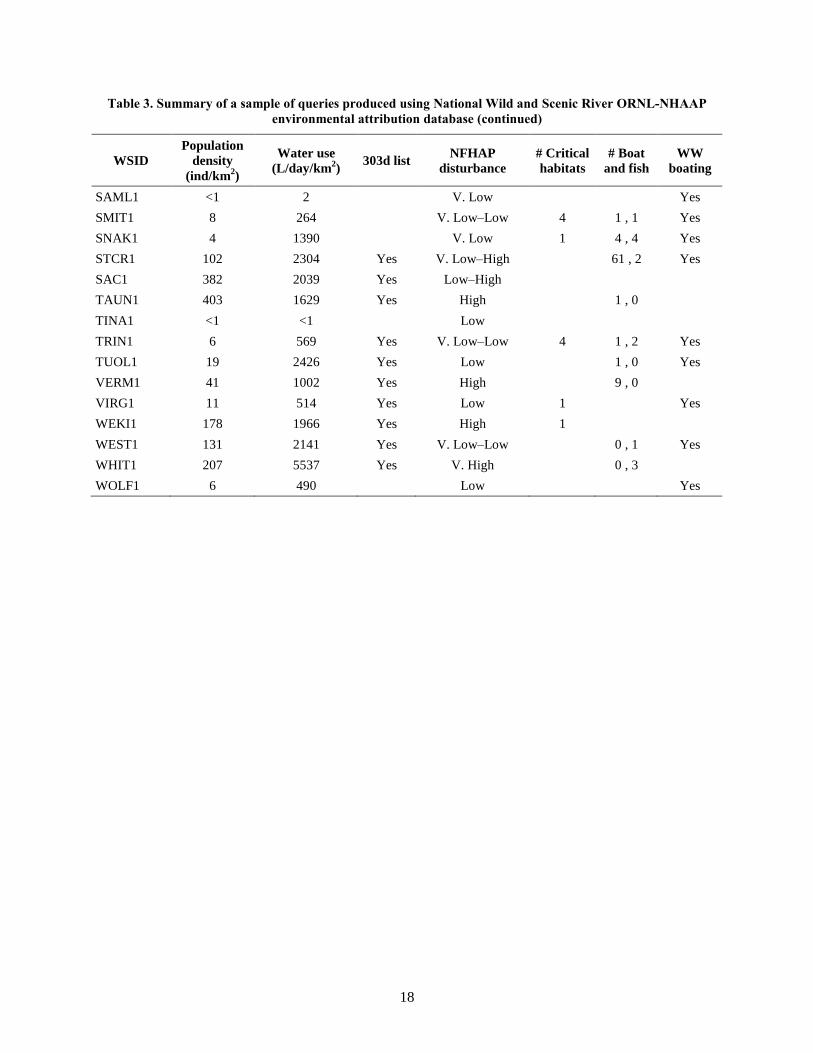
Other queries produced interesting and varied results for WSRs (Table 3). Population density differs

widely, from <1 individual per km2 along several Alaskan rivers to >290 individuals per km

2 along highly

populated river areas (e.g. Loxahatchee River, FL). Water use also is highly variable, ranging from <1 L

per km2 per day (primarily Alaskan rivers) to >20,000 L per km

2 per day in the Little Beaver River

watershed in Ohio (Table 3). However, note that estimates of both population density and water use are

derived from averages for the HUC08 subbasin in which each WSR is located. Thus these are not

accurate estimates of population density adjacent to each river bank or of water use specifically from each

river. However, most WSRs are moderate-to-large river systems spanning from one to multiple HUC08

subbasins. Thus HUC08 subbasins provide an adequate measure of environmental context to provide a

relative comparison among WSRs.

For other environmental variables, a 500 m buffer or NHD catchments were used to assign values to each

WSR. Approximately 55% of all WSRs had mainstem or tributary reaches designated as impaired under

the EPA 303d waterbody listing (Table 3). Disturbance along at least part of the drainage of 13 of the 49

WSRs (26%) was classified as “high,” according to the National Fish Habitat Action Plan habitat

disturbance summary. Endangered Species Act–designated critical habitats for listed endangered and

threatened species were found in 28% of WSRs. Boat ramp and fishing access locations were also

abundant, occurring at 55% of WSRs (Table 3). Finally, according to data from the National Whitewater

Inventory (AW 2013), most WSRs (61%) provide some form of whitewater boating recreation (Table 3).

14

Table 2. Summary of protected lands and primary (majority), second, and third largest land-owning entity within a 500 m buffered acreage around

each WSR

WSID River name Buffered

acreage

Protected

acreage

%

Protected # Entities Majority Second Third

ALAG1 Alaganack River, AK 25,615 25,615 100 5 NPS Private BLM

ALAT1 Alatna River, AK 33,123 33,123 100 2 NPS Private ---

ALLA1 Allagash River, ME 43,747 19,069 44 3 None State Unknown

ANIA1 Aniakchak River, AK 26,730 26,730 100 2 NPS NOAA ---

BLD1 Big and Little Darby Creeks, OH 31,330 3,150 10 4 None County Private

BLSTN1 Bluestone River, WV 7,724 7,217 93 4 NPS State DOD

CLP1 Cache le Poudre River, CO 32,975 29,809 90 8 USFS NPS None

CHAR1 Charley River, AK 87,541 87,532 100 1 NPS --- ---

CHIL1 Chilikadrontna River, AK 7,941 7,941 100 2 NPS State ---

CSL1 Cossatot River, AR 13,196 10,491 80 3 USFS Unknown State

EEL1 Eel River, CA 176,858 54,366 31 9 None USFS State park

8M1 Eight Mile River, CT 8,839 3,731 42 9 None Private Unknown

FARM1 Farmington River, CT 5,598 1,563 28 4 None State DOD

FLTH1 Flathead River, MT 74,047 69,913 94 6 USFS NPS BOR

GREG1 Great Egg Harbor River, NJ 27,645 14,196 51 6 None State NOAA

JOHN1 John River, AK 25,114 25,114 100 3 NPS State Private

KERN1 Kern River, CA 48,410 47,467 98 3 USFS NPS None

KING1 Kings River, CA 34,265 34,262 100 2 NPS USFS ---

KLAM1 Klamath River, CA 74,774 56,380 75 7 USFS None NAM

KOBU1 Kobuk River, AK 41,759 41,759 100 3 NPS Private State

LAMP1 Lamprey River, NH 7,885 1,777 23 7 None Unknown State

LIBE1 Little Beaver River, OH 21,427 3,127 15 1 None State ---

LIMI1 Little Miami River, OH 35,663 3,265 9 4 None State County

LOXA1 Loxahatchee River, FL 5,000 4,540 91 6 State State None

LUMB1 Lumber River, NC 23,286 4,276 18 3 None State Park Private

15

Table 2. Summary of protected lands and primary (majority), second, and third largest land-owning entity within a 500 m buffered acreage around

each WSR (continued)

WSID River name Buffered

acreage

Protected

acreage

%

Protected # Entities Majority Second Third

MAUR1 Maurice River, NJ 9,758 4,170 43 7 None State TNC

MERC1 Merced River, CA 48,462 47,605 98 8 NPS USFS BLM

MISS1 Missouri River, NB & SD 50,858 41,919 82 8 NPS None Private

MULC1 Mulchatna River, AK 9,732 9,732 100 2 NPS State None

MUSC1 Musconetcong River, NJ 10,164 6,405 63 6 None Unknown State

NR1 New River, NC 9,613 1,723 18 2 None State park Private

NFKO1 North Fork Koyuku River, AK 44,145 44,145 100 4 NPS Private Unknown

OB1 Obed River, TN 16,156 11,760 73 2 State NPS None

RIGR1 Rio Grande River, NM 32,366 28,570 88 5 BLM None USFS

SALM1 Salmon River, AK 28,926 28,926 100 2 NPS Private ---

SMIT1 Smith River, CA 47,435 40,074 84 5 USFS None State park

SNAK1 Snake River Headwaters, WY 146,132 140,912 96 7 USFS NPS None

STCR1 St Croix River, MN & WI 138,148 124,254 90 12 NPS Private None

SAC1 SudburyAssabetConcord River, MA 11,507 4,473 39 12 None FWS City

TAUN1 Taunton River, MA 14,726 4,828 33 9 None NOAA State

TINA1 Tinayguk River, AK 20,338 20,338 100 1 NPS --- ---

TRIN1 Trinity River, CA 90,268 70,375 78 6 USFS None NAM

TUOL1 Tuolomne River, CA 29,014 24,643 85 5 NPS USFS None

VERM1 Vermillion River, IL 6,151 4,204 68 3 State None Private

VIRG1 Virgin River, UT 57,812 55,117 95 5 NPS BLM None

WEKI1 Wekiva River, FL 16,401 12,443 76 5 State None L.Gov.

WEST1 Westfield River, MA 31,984 10,482 33 5 None State park State

WHIT1 White Clay Creek, DE & PA 60,585 12,950 21 8 None State park Unknown

WOLF1 Wolf River, WI 9,087 34 < 1 2 None State Private

16

Fig. 5. Eel WSR and adjacent protected lands owned by various agencies falling within a 500 m buffer.

17

Table 3. Summary of a sample of queries produced using National Wild and Scenic River ORNL-NHAAP

environmental attribution database The term “303d” refers to the EPA 303d waterbody listing under the Clean

Water Act. “Boat,” “Fish,” and “WW” refer to boat ramps, fishing access points, and whitewater, respectively.

“Yes” indicates the presence of various attributes; a blank indicates they were not detected

WSID

Population

density

(ind/km2)

Water use

(L/day/km2)

303d list NFHAP

disturbance

# Critical

habitats

# Boat

and fish

WW

boating

ALAG1 <1 1 V. Low–Low

ALAT1 <1 <1 V. Low Yes

ALLA1 6 64 V. Low 1 7 , 1 Yes

ANIA1 <1 2 V. Low Yes

BLD1 105 1408 Yes Mod.–High

BLSTN1 <1 2934 Yes Mod. 3 , 0 Yes

CLP1 32 2692 Low 1 1 , 3 Yes

CHAR1 2 37 Low Yes

CHIL1 <1 <1 V. Low Yes

CSL1 10 145 Mod. Yes

EEL1 11 437 Yes Low 6 0 , 3 Yes

8M1 290 3805 Yes Mod. 0 , 1

FARM1 255 2127 Yes Low Yes

FLAT1 6 515 V. Low–Mod. 2 0 , 3 Yes

GREG1 212 1299 Yes Mod. 0 , 1

JOHN1 <1 <1 Low

KERN1 36 6762 V. Low 0 , 1 Yes

KING1 30 5122 V. Low–Low Yes

KLAM1 6 589 Yes V. Low–High 4 2 , 1 Yes

KOBU1 <1 3 V. Low

LAMP1 111 937 Yes Low

LIBE1 176 20157 Yes High 0 , 1 Yes

LIMI1 120 6263 Yes Mod.–High 2 , 1 Yes

LOXA1 292 3974 Low 1 1 , 0

LUMB1 42 535 Yes Mod. 3 , 0

MAUR1 125 1492 Yes Mod. 1 , 2

MERC1 26 4724 V. Low–Low Yes

MISS1 5 667 Yes Mod.–High 1 11 , 5

MULC1 <1 <1 V. Low

MUSC1 244 6928 Yes V. High 0 , 1 Yes

NR1 30 276 Yes High 2 , 1 Yes

NFKO1 <1 <1 Low

OB1 23 2886 Yes Low 2 Yes

RIGR1 6 2683 Yes Low 1 0 , 2 Yes

18

Table 3. Summary of a sample of queries produced using National Wild and Scenic River ORNL-NHAAP

environmental attribution database (continued)

WSID

Population

density

(ind/km2)

Water use

(L/day/km2)

303d list NFHAP

disturbance

# Critical

habitats

# Boat

and fish

WW

boating

SAML1 <1 2 V. Low Yes

SMIT1 8 264 V. Low–Low 4 1 , 1 Yes

SNAK1 4 1390 V. Low 1 4 , 4 Yes

STCR1 102 2304 Yes V. Low–High 61 , 2 Yes

SAC1 382 2039 Yes Low–High

TAUN1 403 1629 Yes High 1 , 0

TINA1 <1 <1 Low

TRIN1 6 569 Yes V. Low–Low 4 1 , 2 Yes

TUOL1 19 2426 Yes Low 1 , 0 Yes

VERM1 41 1002 Yes High 9 , 0

VIRG1 11 514 Yes Low 1 Yes

WEKI1 178 1966 Yes High 1

WEST1 131 2141 Yes V. Low–Low 0 , 1 Yes

WHIT1 207 5537 Yes V. High 0 , 3

WOLF1 6 490 Low Yes

19

4. DISCUSSION

This report provides a methodology for accurately mapping WSRs to support geospatial analyses. The

digital mapping of WSRs was followed by an environmental characterization of each river system to

determine whether consistent environmental patterns were evident for WSRs across the nation. The

spatial scale of hydrography datasets and adherence to written policy descriptions are both critical to

accurately mapping WSR resources. Although policy descriptions were sufficient to demarcate the

upstream and downstream extent of many rivers, other descriptions rendered interpretation difficult. This

issue suggests potential losses in the accurate spatial representation of each waterbody. In addition, the

total river mileage reported as protected under WSRs is influenced by the underlying hydrography dataset

and interpretation used to determine the extent of protection. The environmental characterization provided

information to deduce generalized trends in the uniqueness or commonness of environmental qualities in

WSRs. It is interesting that watersheds containing WSRs represent a large range of landscape conditions,

from pristine areas to highly modified landscapes. For example, 303d listed waterbodies were prevalent,

riparian zones had inconsistent protection, and population size and water use were, at times, very high.

However, 28% of WSRs contained critical habitats and almost 80% were documented as supporting some

type of aquatic recreation. Altogether, these data suggest that despite inconsistencies in the status of

surrounding landscapes, WSRs provide habitats important to aquatic organisms and recreational

opportunities important to humans. However, note also that much of the ecological uniqueness and

aesthetic importance of WSRs is not captured in this analysis.

The research findings suggest a need for accurate mapping of WSRs for public use. However, results also

suggest that methodologies for mapping WSRs should also be consistent. Besides the NPS, the USFS,

FWS, and BLM have jurisdiction over WSRs. Since different agencies are responsible for mapping their

own assets, the potential exists for large discrepancies in the resultant national layer. Different underlying

hydrographic layers, projections, and interpretations could result in large disparities in spatial

representation in the final result. Another complication is that multiple agencies may be responsible for a

single river. The spatial representation of layers extends beyond just mapping exercises. Federal, state,

and local governments rely on accurate spatial representations in planning for development before on-the-

ground visits. Geospatial applications are required to provide relatively accurate estimates of renewable

and sustainable energy development at the scale of the entire United States to support federal policy. As

much as 20% of energy capacity from new potential hydropower development in the conterminous United

States could overlap with WSRs (ORNL 2013). However, this estimate was based upon the prevailing

geospatial coverage of WSRs created using the 1:2M scale USGS hydrography layer. Therefore, analyses

examining areas of potential development require data layers with precise spatial representation and high

spatial accuracy.

5. REFERENCES

AW (American Whitewater). 2013. National Whitewater Inventory. Accessed August 30, 2013 at:

http://www.americanwhitewater.org/content/River/view/

Hadjerioua, B., S-C Kao, R.A. McManamay, M.D. Fayzul, K. Pasha, D. Yeasmin, A.A. Oubeidillah,

N.M. Samu, K.M. Stewart, M.S. Bevelhimer, S.L. Hetrick, Y. Wei, and B.T. Smith. 2012. An

assessment of energy potential from new small hydro development in the United States. Initial Report

on Methodology. Report by Oak Ridge National Laboratory to the Department of Energy. August,

2012. http://nhaap.ornl.gov/sites/default/files/NSD_Methodology_Report.pdf

National Atlas. 2013. Two Million-Scale Streams and Waterbodies. Accessed August 30, 2013 at:

http://nationalatlas.gov/mld/hydrogm.html

NPS (National Park Service). 2013. Wild and Scenic Rivers. Accessed August 29, 2013 at:

http://www.nature.nps.gov/water/wild_scenic_rivers/

NWSRS (National Wild and Scenic River System). 2013. National Wild and Scenic River System.

Accessed August 30, 2013 at: http://www.rivers.gov/

ORNL (Oak Ridge National Laboratory). 2013. New Stream Reach Development Potential. National

Hydropower Asset Assessment Program. Accessed August 30, 2013 at: http://nhaap.ornl.gov/

USGS (US Geological Survey). 2013a. National Hydography Dataset. Accessed August 29, 2013 at:

http://nhd.usgs.gov/index.html

USGS (US Geological Survey). 2013b. NHD Tools. Accessed August 29, 2013 at:

http://nhd.usgs.gov/tools.html

WSRA (Wild and Scenic Rivers Act). 1968. Wild & Scenic Rivers Act (16 U.S.C. 1271-1287). Public

Law 90-542. October 2, 1968. Washington, D.C.