Scilab Textbook Companion for Digital Image Processing by S. Jayaraman, S. Esakkirajan And T. Veerakumar 1 Created by R.Senthilkumar M.E., Assistant Professor Electronics Engineering Inst. of Road and Transport Tech., Erode College Teacher Dr. R.K.Gnanamurhty, Principal,V. C. E. W. Cross-Checked by Anuradha Amrutkar, IIT Bombay August 10, 2013 1 Funded by a grant from the National Mission on Education through ICT, http://spoken-tutorial.org/NMEICT-Intro. This Textbook Companion and Scilab codes written in it can be downloaded from the ”Textbook Companion Project” section at the website http://scilab.in

Digital Image Processing_S. Jayaraman, S. Esakkirajan and T. Veerakumar
Oct 23, 2015
Welcome message from author
This document is posted to help you gain knowledge. Please leave a comment to let me know what you think about it! Share it to your friends and learn new things together.
Transcript
Scilab Textbook Companion forDigital Image Processing
by S. Jayaraman, S. Esakkirajan And T.Veerakumar1
Created byR.Senthilkumar
M.E., Assistant ProfessorElectronics Engineering
Inst. of Road and Transport Tech., ErodeCollege Teacher
Dr. R.K.Gnanamurhty, Principal,V. C. E. W.Cross-Checked by
Anuradha Amrutkar, IIT Bombay
August 10, 2013
1Funded by a grant from the National Mission on Education through ICT,http://spoken-tutorial.org/NMEICT-Intro. This Textbook Companion and Scilabcodes written in it can be downloaded from the ”Textbook Companion Project”section at the website http://scilab.in

Book Description
Title: Digital Image Processing
Author: S. Jayaraman, S. Esakkirajan And T. Veerakumar
Publisher: Tata McGraw - Hill Education Pvt. Ltd, New Delhi
Edition: 3
Year: 2010
ISBN: 978-0-07-014479-8
1
Scilab numbering policy used in this document and the relation to theabove book.
Exa Example (Solved example)
Eqn Equation (Particular equation of the above book)
AP Appendix to Example(Scilab Code that is an Appednix to a particularExample of the above book)
For example, Exa 3.51 means solved example 3.51 of this book. Sec 2.3 meansa scilab code whose theory is explained in Section 2.3 of the book.
2

Contents
List of Scilab Codes 4
1 Introduction to Image Processing System 9
2 2D Signals and Systems 12
3 Convolution and Correlation 15
4 Image Transforms 24
5 Image Enhancement 34
6 Image Restoration and Denoising 44
7 Image Segmentation 64
8 Object Recognition 73
9 Image Compression 77
10 Binary Image Processing 81
11 Colur Image Processing 85
12 Wavelet based Image Processing 99
3

List of Scilab Codes
Exa 1.3 Program to calculate number of samples required for animage . . . . . . . . . . . . . . . . . . . . . . . . . . . 9
Exa 1.13 False contouring Scilab code . . . . . . . . . . . . . . . 10Exa 2.12 Frequency Response . . . . . . . . . . . . . . . . . . . 12Exa 2.16 Frequency Response . . . . . . . . . . . . . . . . . . . 12Exa 3.1 2D Linear Convlolution . . . . . . . . . . . . . . . . . 15Exa 3.2 2D Linear Convolution . . . . . . . . . . . . . . . . . . 15Exa 3.3 2D Linear Convolution . . . . . . . . . . . . . . . . . . 16Exa 3.7 2D Linear Convolution . . . . . . . . . . . . . . . . . . 17Exa 3.8 2D Linear Convolution . . . . . . . . . . . . . . . . . . 17Exa 3.11 Linear Convolution of any signal with an impule signal
given rise to the same signal . . . . . . . . . . . . . . . 18Exa 3.12 Circular Convolution between two 2D matrices . . . . 18Exa 3.13 Circular Convolution exspressed as linear convolution
plus alias . . . . . . . . . . . . . . . . . . . . . . . . . 19Exa 3.14 Linear Cross correlation of a 2D matrix . . . . . . . . 20Exa 3.15 Circular correlation between two signals . . . . . . . . 20Exa 3.16 Circular correlation between two signals . . . . . . . . 21Exa 3.17 Linear auto correlation of a 2D matrix . . . . . . . . . 22Exa 3.18 Linear Cross correlation of a 2D matrix . . . . . . . . 22Exa 4.4 DFT of 4x4 grayscale image . . . . . . . . . . . . . . . 24Exa 4.5 2D DFT of 4X4 grayscale image . . . . . . . . . . . . 24Exa 4.6 Scilab code to intergchange phase information between
two images . . . . . . . . . . . . . . . . . . . . . . . . 25Exa 4.10 Program to compute discrete cosine transform . . . . . 26Exa 4.12 Program to perform KL tranform for the given 2D matrix 28Exa 4.13 Program to find the singular value decomposition of
given matrix . . . . . . . . . . . . . . . . . . . . . . . 32
4

Exa 5.5 Scilab code for brightness enhancement . . . . . . . . 34Exa 5.7 Scilab code for brightness suppression . . . . . . . . . 36Exa 5.9 Scilab code for Contrast Manipulation . . . . . . . . . 36Exa 5.13 Scilab code to determine image negative . . . . . . . . 38Exa 5.16 Scilab code that performs threshold operation . . . . . 38Exa 5.20 Program performs gray level slicing without background 40Exa 6.1 Scilab code to create motion blur . . . . . . . . . . . . 44Exa 6.5 Scilab code performs inverse filtering . . . . . . . . . . 45Exa 6.7 Scilab code performs inverse filtering . . . . . . . . . . 48Exa 6.9 Scilab code performs Pseudo inverse filtering . . . . . 50Exa 6.13 Scilab code to perform wiener filtering of the corrupted
image . . . . . . . . . . . . . . . . . . . . . . . . . . . 54Exa 6.18 Scilab code to Perform Average Filtering operation . . 55Exa 6.21 Scilab code to Perform median filtering . . . . . . . . 57Exa 6.23 Scilab code to Perform median filtering of colour image 59Exa 6.24 Scilab code to Perform Trimmed Average Filter . . . . 61Exa 7.23 Scilab code for Differentiation of Gaussian function . . 64Exa 7.25 Scilab code for Differentiation of Gaussian Filter function 67Exa 7.27 Scilab code for Edge Detection using Different Edge de-
tectors . . . . . . . . . . . . . . . . . . . . . . . . . . . 69Exa 7.30 Scilab code to perform watershed transform . . . . . . 71Exa 8.4 To verify the given matrix is a covaraince matrix . . . 73Exa 8.5 To compute the covariance of the given 2D data . . . 73Exa 8.9 Develop a perceptron AND function with bipolar inputs
and targets . . . . . . . . . . . . . . . . . . . . . . . . 75Exa 9.9 Program performs Block Truncation Coding BTC . . . 77Exa 9.59 Program performs Block Truncation Coding . . . . . . 79Exa 10.17 Scilab Code for dilation and erosion process . . . . . . 81Exa 10.19 Scilab Code to perform an opening and closing opera-
tion on the image . . . . . . . . . . . . . . . . . . . . 82Exa 11.4 Read an RGB image and extract the three colour com-
ponents red green blue . . . . . . . . . . . . . . . . . . 85Exa 11.12 Read a Colour image and separate the colour image into
red green and blue planes . . . . . . . . . . . . . . . . 86Exa 11.16 Compute the histogram of the colour image . . . . . . 88Exa 11.18 Perform histogram equalisation of the given RGB image 90Exa 11.21 This program performs median filtering of the colour
image . . . . . . . . . . . . . . . . . . . . . . . . . . . 91
5
Exa 11.24 Fitlering only the luminance component . . . . . . . . 92Exa 11.28 Perform gamma correction for the given colour image . 93Exa 11.30 Perform Pseudo Colouring Operation . . . . . . . . . . 95Exa 11.32 Read an RGB image and segment it using the threshold
method . . . . . . . . . . . . . . . . . . . . . . . . . . 96Exa 12.9 Scilab code to perform wavelet decomposition . . . . . 99Exa 12.42 Scilab code to generate different levels of a Gaussian
pyramid . . . . . . . . . . . . . . . . . . . . . . . . . . 100Exa 12.57 Scilab code to implement watermarking in spatial domain 101Exa 12.63 Scilab code to implement wavelet based watermarking 104AP 1 2D Fast Fourier Transform . . . . . . . . . . . . . . . 107AP 2 2D Inverse FFT . . . . . . . . . . . . . . . . . . . . . 108AP 3 Median Filtering function . . . . . . . . . . . . . . . . 108AP 4 To caculate gray level . . . . . . . . . . . . . . . . . . 109AP 5 To change the gray level of gray image . . . . . . . . . 109
6

List of Figures
1.1 False contouring Scilab code . . . . . . . . . . . . . . . . . . 11
2.1 Frequency Response . . . . . . . . . . . . . . . . . . . . . . 132.2 Frequency Response . . . . . . . . . . . . . . . . . . . . . . 14
4.1 Scilab code to intergchange phase information between twoimages . . . . . . . . . . . . . . . . . . . . . . . . . . . . . . 27
4.2 Program to compute discrete cosine transform . . . . . . . . 294.3 Program to compute discrete cosine transform . . . . . . . . 30
5.1 Scilab code for brightness enhancement . . . . . . . . . . . . 355.2 Scilab code for brightness suppression . . . . . . . . . . . . . 375.3 Scilab code for Contrast Manipulation . . . . . . . . . . . . 395.4 Scilab code to determine image negative . . . . . . . . . . . 395.5 Scilab code that performs threshold operation . . . . . . . . 415.6 Program performs gray level slicing without background . . 43
6.1 Scilab code to create motion blur . . . . . . . . . . . . . . . 456.2 Scilab code performs inverse filtering . . . . . . . . . . . . . 476.3 Scilab code performs inverse filtering . . . . . . . . . . . . . 496.4 Scilab code performs inverse filtering . . . . . . . . . . . . . 516.5 Scilab code performs Pseudo inverse filtering . . . . . . . . . 536.6 Scilab code to perform wiener filtering of the corrupted image 566.7 Scilab code to Perform Average Filtering operation . . . . . 586.8 Scilab code to Perform median filtering . . . . . . . . . . . . 606.9 Scilab code to Perform median filtering of colour image . . . 616.10 Scilab code to Perform Trimmed Average Filter . . . . . . . 63
7.1 Scilab code for Differentiation of Gaussian function . . . . . 657.2 Scilab code for Differentiation of Gaussian function . . . . . 66
7
7.3 Scilab code for Differentiation of Gaussian Filter function . . 677.4 Scilab code for Differentiation of Gaussian Filter function . . 687.5 Scilab code for Edge Detection using Different Edge detectors 707.6 Scilab code to perform watershed transform . . . . . . . . . 72
9.1 Program performs Block Truncation Coding . . . . . . . . . 80
10.1 Scilab Code for dilation and erosion process . . . . . . . . . 8210.2 Scilab Code to perform an opening and closing operation on
the image . . . . . . . . . . . . . . . . . . . . . . . . . . . . 84
11.1 Read an RGB image and extract the three colour componentsred green blue . . . . . . . . . . . . . . . . . . . . . . . . . . 87
11.2 Read a Colour image and separate the colour image into redgreen and blue planes . . . . . . . . . . . . . . . . . . . . . . 89
11.3 This program performs median filtering of the colour image . 9211.4 Fitlering only the luminance component . . . . . . . . . . . 9411.5 Perform gamma correction for the given colour image . . . . 9511.6 Perform Pseudo Colouring Operation . . . . . . . . . . . . . 9711.7 Read an RGB image and segment it using the threshold method 98
12.1 Scilab code to generate different levels of a Gaussian pyramid 10212.2 Scilab code to implement watermarking in spatial domain . . 104
8
Chapter 1
Introduction to ImageProcessing System
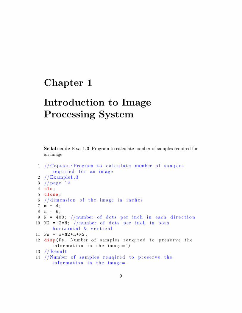
Scilab code Exa 1.3 Program to calculate number of samples required foran image
1 // Capt ion : Program to c a l c u l a t e number o f sample sr e q u i r e d f o r an image
2 // Example1 . 33 // page 124 clc;
5 close;
6 // d imens ion o f the image i n i n c h e s7 m = 4;
8 n = 6;
9 N = 400; // number o f do t s per i n ch i n each d i r e c t i o n10 N2 = 2*N; // number o f do t s per i n ch i n both
h o r i z o n t a l & v e r t i c a l11 Fs = m*N2*n*N2;
12 disp(Fs, ’ Number o f sample s r e u q i r e d to p r e s e r v e thei n f o r m a t i o n i n the image= ’ )
13 // R e s u l t14 //Number o f sample s r e u q i r e d to p r e s e r v e the
i n f o r m a t i o n i n the image=
9
15 // 1 5 3 6 0 0 00 .
check Appendix AP 4 for dependency:
gray.sci
check Appendix AP 5 for dependency:
grayslice.sci
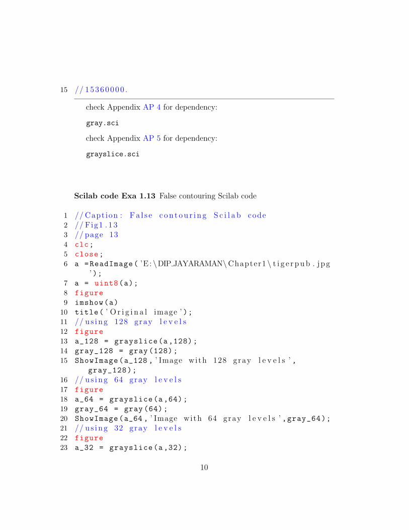
Scilab code Exa 1.13 False contouring Scilab code
1 // Capt ion : F a l s e c o n t o u r i n g S c i l a b code2 // Fig1 . 1 33 // page 134 clc;
5 close;
6 a =ReadImage( ’E : \DIP JAYARAMAN\Chapter1 \ t i g e r p u b . jpg’ );
7 a = uint8(a);
8 figure
9 imshow(a)
10 title( ’ O r i g i n a l image ’ );11 // u s i n g 128 gray l e v e l s12 figure
13 a_128 = grayslice(a,128);
14 gray_128 = gray (128);
15 ShowImage(a_128 , ’ Image with 128 gray l e v e l s ’ ,gray_128);
16 // u s i n g 64 gray l e v e l s17 figure
18 a_64 = grayslice(a,64);
19 gray_64 = gray (64);
20 ShowImage(a_64 , ’ Image with 64 gray l e v e l s ’ ,gray_64);21 // u s i n g 32 gray l e v e l s22 figure
23 a_32 = grayslice(a,32);
10

Figure 1.1: False contouring Scilab code
24 gray_32 = gray (32);
25 ShowImage(a_32 , ’ Image with 32 gray l e v e l s ’ ,gray_32);26 // u s i n g 16 gray l e v e l s27 figure
28 a_16 = grayslice(a,16);
29 gray_16 = gray (16);
30 ShowImage(a_16 , ’ Image with 16 gray l e v e l s ’ ,gray_16);31 // u s i n g 8 gray l e v e l s32 a_8 = grayslice(a,8);
33 gray_8 = gray (8);
34 ShowImage(a_8 , ’ Image with 8 gray l e v e l s ’ ,gray_8);
11

Chapter 2
2D Signals and Systems
Scilab code Exa 2.12 Frequency Response
1 // Capt ion : Frequency Response2 // Fig2 . 1 23 // page 604 clc;
5 close;
6 [X, Y] = meshgrid(-%pi :.09: %pi);
7 Z = 2*cos(X)+2* cos(Y);
8 surf(X,Y,Z);
9 xgrid (1)
Scilab code Exa 2.16 Frequency Response
1 // Capt ion : Frequency Response2 // Fig2 . 1 63 // page 64
12
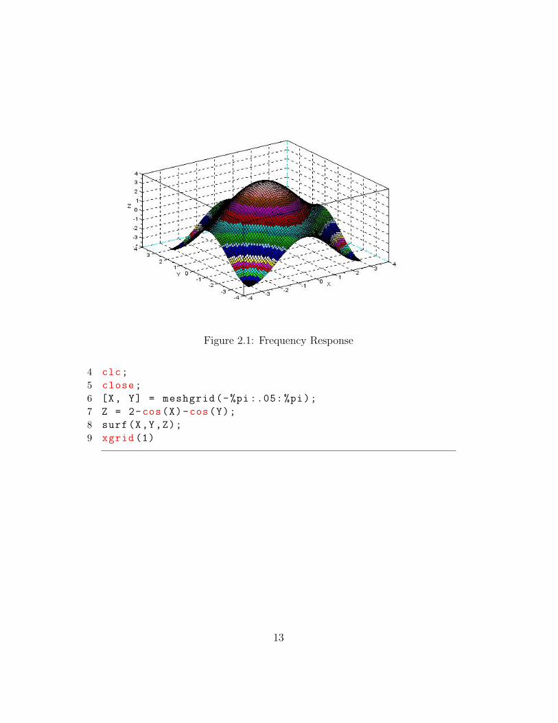
Figure 2.1: Frequency Response
4 clc;
5 close;
6 [X, Y] = meshgrid(-%pi :.05: %pi);
7 Z = 2-cos(X)-cos(Y);
8 surf(X,Y,Z);
9 xgrid (1)
13

Figure 2.2: Frequency Response
14
Chapter 3
Convolution and Correlation
Scilab code Exa 3.1 2D Linear Convlolution
1 // Capt ion : 2−D L i n e a r Convo lu t i on2 // Example3 . 1 & Example3 . 43 // page 85 & page 1074 clc;
5 x =[4,5,6;7,8 ,9];
6 h = [1;1;1];
7 disp(x, ’ x= ’ )8 disp(h, ’ h= ’ )9 [y,X,H] = conv2d2(x,h);
10 disp(y, ’ L i n e a r 2D c o n v o l u t i o n r e s u l t y = ’ )11 // R e s u l t12 // L i n e a r 2D c o n v o l u t i o n r e s u l t y =13 //14 // 4 . 5 . 6 .15 // 1 1 . 1 3 . 1 5 .16 // 1 1 . 1 3 . 1 5 .17 // 7 . 8 . 9 .
Scilab code Exa 3.2 2D Linear Convolution
15
1 // Capt ion : 2−D L i n e a r Convo lu t i on2 // Example3 . 2 & Example3 . 5 & Example3 . 93 // page 91 & page 108 & page 1164 clc;
5 x =[1,2,3;4,5,6;7 ,8,9];
6 h = [1 ,1;1 ,1;1 ,1];
7 y = conv2d2(x,h);
8 disp(y, ’ L i n e a r 2D c o n v o l u t i o n r e s u l t y = ’ )9 // R e s u l t
10 // L i n e a r 2D c o n v o l u t i o n r e s u l t y =11 //12 // 1 . 3 . 5 . 3 .13 // 5 . 1 2 . 1 6 . 9 .14 // 1 2 . 2 7 . 3 3 . 1 8 .15 // 1 1 . 2 4 . 2 8 . 1 5 .16 // 7 . 1 5 . 1 7 . 9 .17 //
Scilab code Exa 3.3 2D Linear Convolution
1 // Capt ion : 2−D L i n e a r Convo lu t i on2 // Example3 . 3 & Example3 . 6 & Example3 . 1 03 // page 100 & page 109 & page 1194 clc;
5 x =[1,2,3;4,5 ,6;7 ,8,9];
6 h = [3,4,5];
7 y = conv2d2(x,h);
8 disp(y, ’ L i n e a r 2D c o n v o l u t i o n r e s u l t y = ’ )9 // R e s u l t
10 // L i n e a r 2D c o n v o l u t i o n r e s u l t y =11 //12 // 3 . 1 0 . 2 2 . 2 2 . 1 5 .13 // 1 2 . 3 1 . 5 8 . 4 9 . 3 0 .14 // 2 1 . 5 2 . 9 4 . 7 6 . 4 5 .
16
Scilab code Exa 3.7 2D Linear Convolution
1 // Capt ion : 2−D L i n e a r Convo lu t i on2 // Example3 . 73 // page 1114 clc;
5 x =[1 ,2;3 ,4];
6 h = [5 ,6;7 ,8];
7 y = conv2d2(x,h);
8 disp(y, ’ L i n e a r 2D c o n v o l u t i o n r e s u l t y = ’ )9 // R e s u l t
10 // L i n e a r 2D c o n v o l u t i o n r e s u l t y =11 // L i n e a r 2D c o n v o l u t i o n r e s u l t y =12 //13 // 5 . 1 6 . 1 2 .14 // 2 2 . 6 0 . 4 0 .15 // 2 1 . 5 2 . 32
Scilab code Exa 3.8 2D Linear Convolution
1 // Capt ion : 2−D L i n e a r Convo lu t i on2 // Example3 . 83 // page 1134 clc;
5 x =[1,2,3;4,5 ,6;7 ,8,9];
6 h = [1;1;1];
7 y = conv2d2(x,h);
8 disp(y, ’ L i n e a r 2D c o n v o l u t i o n r e s u l t y = ’ )9 // R e s u l t
10 // L i n e a r 2D c o n v o l u t i o n r e s u l t y =11 // // 1 . 2 . 3 .12 // 5 . 7 . 9 .
17
13 // 1 2 . 1 5 . 1 8 .14 // 1 1 . 1 3 . 1 5 .15 // 7 . 8 . 9 .
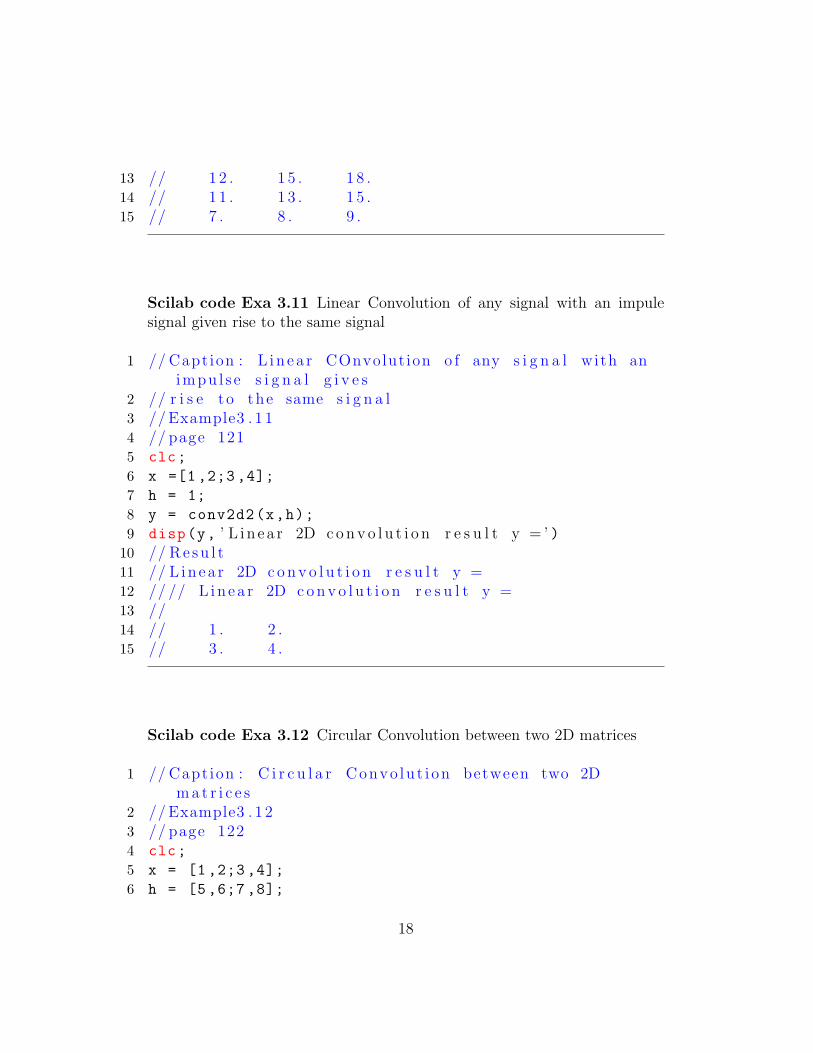
Scilab code Exa 3.11 Linear Convolution of any signal with an impulesignal given rise to the same signal
1 // Capt ion : L i n e a r COnvolut ion o f any s i g n a l with animpu l s e s i g n a l g i v e s
2 // r i s e to the same s i g n a l3 // Example3 . 1 14 // page 1215 clc;
6 x =[1 ,2;3 ,4];
7 h = 1;
8 y = conv2d2(x,h);
9 disp(y, ’ L i n e a r 2D c o n v o l u t i o n r e s u l t y = ’ )10 // R e s u l t11 // L i n e a r 2D c o n v o l u t i o n r e s u l t y =12 // // L i n e a r 2D c o n v o l u t i o n r e s u l t y =13 //14 // 1 . 2 .15 // 3 . 4 .
Scilab code Exa 3.12 Circular Convolution between two 2D matrices
1 // Capt ion : C i r c u l a r Convo lu t i on between two 2Dm a t r i c e s
2 // Example3 . 1 23 // page 1224 clc;
5 x = [1 ,2;3 ,4];
6 h = [5 ,6;7 ,8];
18
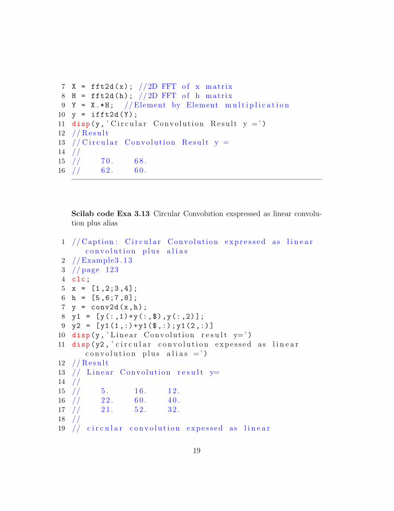
7 X = fft2d(x); // 2D FFT o f x matr ix8 H = fft2d(h); // 2D FFT o f h matr ix9 Y = X.*H; // Element by Element m u l t i p l i c a t i o n
10 y = ifft2d(Y);
11 disp(y, ’ C i r c u l a r Convo lu t i on R e s u l t y = ’ )12 // R e s u l t13 // C i r c u l a r Convo lu t i on R e s u l t y =14 //15 // 7 0 . 6 8 .16 // 6 2 . 6 0 .
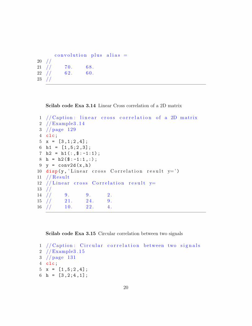
Scilab code Exa 3.13 Circular Convolution exspressed as linear convolu-tion plus alias
1 // Capt ion : C i r c u l a r Convo lu t i on e x p r e s s e d as l i n e a rc o n v o l u t i o n p l u s a l i a s
2 // Example3 . 1 33 // page 1234 clc;
5 x = [1 ,2;3 ,4];
6 h = [5 ,6;7 ,8];
7 y = conv2d(x,h);
8 y1 = [y(:,1)+y(:,$),y(:,2)];
9 y2 = [y1(1,:)+y1($,:);y1(2,:)]
10 disp(y, ’ L i n e a r Convo lu t i on r e s u l t y= ’ )11 disp(y2, ’ c i r c u l a r c o n v o l u t i o n e x p e s s e d as l i n e a r
c o n v o l u t i o n p l u s a l i a s = ’ )12 // R e s u l t13 // L i n e a r Convo lu t i on r e s u l t y=14 //15 // 5 . 1 6 . 1 2 .16 // 2 2 . 6 0 . 4 0 .17 // 2 1 . 5 2 . 3 2 .18 //19 // c i r c u l a r c o n v o l u t i o n e x p e s s e d as l i n e a r
19
c o n v o l u t i o n p l u s a l i a s =20 //21 // 7 0 . 6 8 .22 // 6 2 . 6 0 .23 //
Scilab code Exa 3.14 Linear Cross correlation of a 2D matrix
1 // Capt ion : l i n e a r c r o s s c o r r e l a t i o n o f a 2D matr ix2 // Example3 . 1 43 // page 1294 clc;
5 x = [3 ,1;2 ,4];
6 h1 = [1 ,5;2 ,3];
7 h2 = h1(:,$:-1:1);
8 h = h2($:-1:1,:);
9 y = conv2d(x,h)
10 disp(y, ’ L i n e a r c r o s s C o r r e l a t i o n r e s u l t y= ’ )11 // R e s u l t12 // L i n e a r c r o s s C o r r e l a t i o n r e s u l t y=13 //14 // 9 . 9 . 2 .15 // 2 1 . 2 4 . 9 .16 // 1 0 . 2 2 . 4 .
Scilab code Exa 3.15 Circular correlation between two signals
1 // Capt ion : C i r c u l a r c o r r e l a t i o n between two s i g n a l s2 // Example3 . 1 53 // page 1314 clc;
5 x = [1 ,5;2 ,4];
6 h = [3 ,2;4 ,1];
20

7 h = h(:,$:-1:1);
8 h = h($:-1:1,:);
9 X = fft2d(x);
10 H = fft2d(h);
11 Y = X.*H;
12 y = ifft2d(Y);
13 disp(y, ’ C i r c u l a r C o r r e l a t i o n r e s u l t y= ’ )14 // R e s u l t15 // C i r c u l a r C o r r e l a t i o n r e s u l t y=16 //17 // 3 7 . 2 3 .18 // 3 5 . 2 5 .
Scilab code Exa 3.16 Circular correlation between two signals
1 // Capt ion : C i r c u l a r c o r r e l a t i o n between two s i g n a l s2 // Example3 . 1 63 // page 1344 clc;
5 x = [5 ,10;15 ,20];
6 h = [3 ,6;9 ,12];
7 h = h(:,$:-1:1);
8 h = h($:-1:1,:);
9 X = fft2d(x);
10 H = fft2d(h);
11 Y = X.*H;
12 y = ifft2d(Y);
13 disp(y, ’ C i r c u l a r C o r r e l a t i o n r e s u l t y= ’ )14 // R e s u l t15 // C i r c u l a r C o r r e l a t i o n r e s u l t y=16 //17 // 3 0 0 . 3 3 0 .18 // 4 2 0 . 4 5 0 .
21

Scilab code Exa 3.17 Linear auto correlation of a 2D matrix
1 // Capt ion : l i n e a r auto c o r r e l a t i o n o f a 2D matr ix2 // Example3 . 1 73 // page 1364 clc;
5 x1 = [1 ,1;1 ,1];
6 x2 = x1(:,$:-1:1);
7 x2 = x2($:-1:1,:);
8 x = conv2d(x1,x2)
9 disp(x, ’ L i n e a r auto C o r r e l a t i o n r e s u l t x= ’ )10 // R e s u l t11 // L i n e a r auto C o r r e l a t i o n r e s u l t x=12 //13 // 1 . 2 . 1 .14 // 2 . 4 . 2 .15 // 1 . 2 . 1 .
Scilab code Exa 3.18 Linear Cross correlation of a 2D matrix
1 // Capt ion : l i n e a r c r o s s c o r r e l a t i o n o f a 2D matr ix2 // Example3 . 1 83 // page 1414 clc;
5 x = [1 ,1;1 ,1];
6 h1 = [1 ,2;3 ,4];
7 h2 = h1(:,$:-1:1);
8 h = h2($:-1:1,:);
9 y = conv2d(x,h)
10 disp(y, ’ L i n e a r c r o s s C o r r e l a t i o n r e s u l t y= ’ )11 // R e s u l t12 // L i n e a r c r o s s C o r r e l a t i o n r e s u l t y=
22

13 //14 // 4 . 7 . 3 .15 // 6 . 1 0 . 4 .16 // 2 . 3 . 1 .
23
Chapter 4
Image Transforms
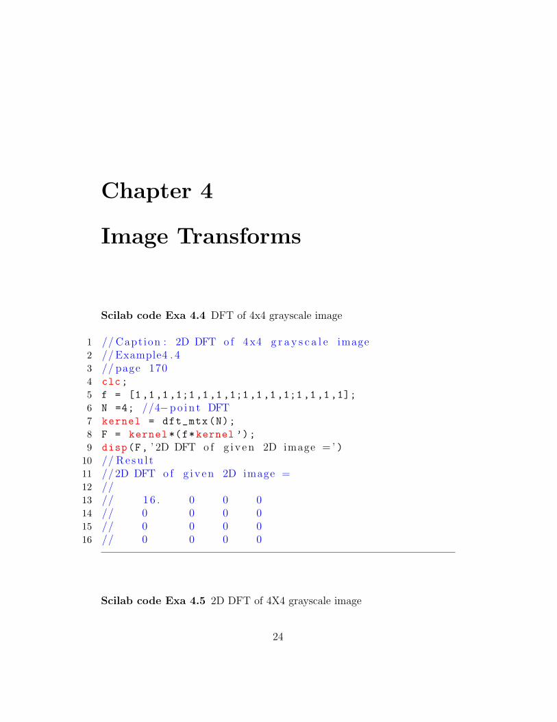
Scilab code Exa 4.4 DFT of 4x4 grayscale image
1 // Capt ion : 2D DFT o f 4 x4 g r a y s c a l e image2 // Example4 . 43 // page 1704 clc;
5 f = [1,1,1,1;1,1,1,1;1,1,1,1;1,1,1,1];
6 N =4; //4−p o i n t DFT7 kernel = dft_mtx(N);
8 F = kernel *(f*kernel ’);
9 disp(F, ’ 2D DFT o f g i v e n 2D image = ’ )10 // R e s u l t11 // 2D DFT o f g i v e n 2D image =12 //13 // 1 6 . 0 0 014 // 0 0 0 015 // 0 0 0 016 // 0 0 0 0
Scilab code Exa 4.5 2D DFT of 4X4 grayscale image
24
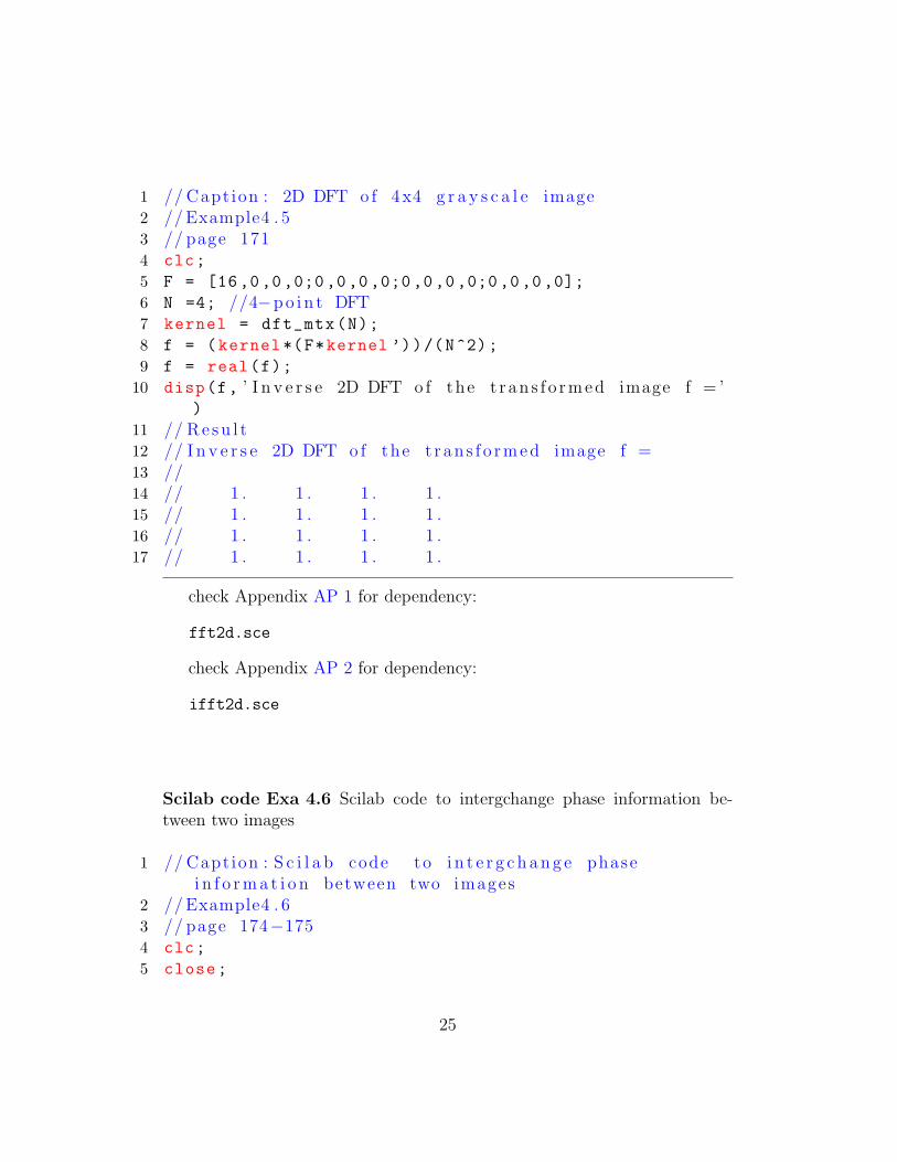
1 // Capt ion : 2D DFT o f 4 x4 g r a y s c a l e image2 // Example4 . 53 // page 1714 clc;
5 F = [16,0,0,0;0,0,0,0;0,0,0,0;0,0,0,0];
6 N =4; //4−p o i n t DFT7 kernel = dft_mtx(N);
8 f = (kernel *(F*kernel ’))/(N^2);
9 f = real(f);
10 disp(f, ’ I n v e r s e 2D DFT o f the t r a n s f o r m e d image f = ’)
11 // R e s u l t12 // I n v e r s e 2D DFT o f the t r a n s f o r m e d image f =13 //14 // 1 . 1 . 1 . 1 .15 // 1 . 1 . 1 . 1 .16 // 1 . 1 . 1 . 1 .17 // 1 . 1 . 1 . 1 .
check Appendix AP 1 for dependency:
fft2d.sce
check Appendix AP 2 for dependency:
ifft2d.sce
Scilab code Exa 4.6 Scilab code to intergchange phase information be-tween two images
1 // Capt ion : S c i l a b code to i n t e r g c h a n g e phasei n f o r m a t i o n between two images
2 // Example4 . 63 // page 174−1754 clc;
5 close;
25
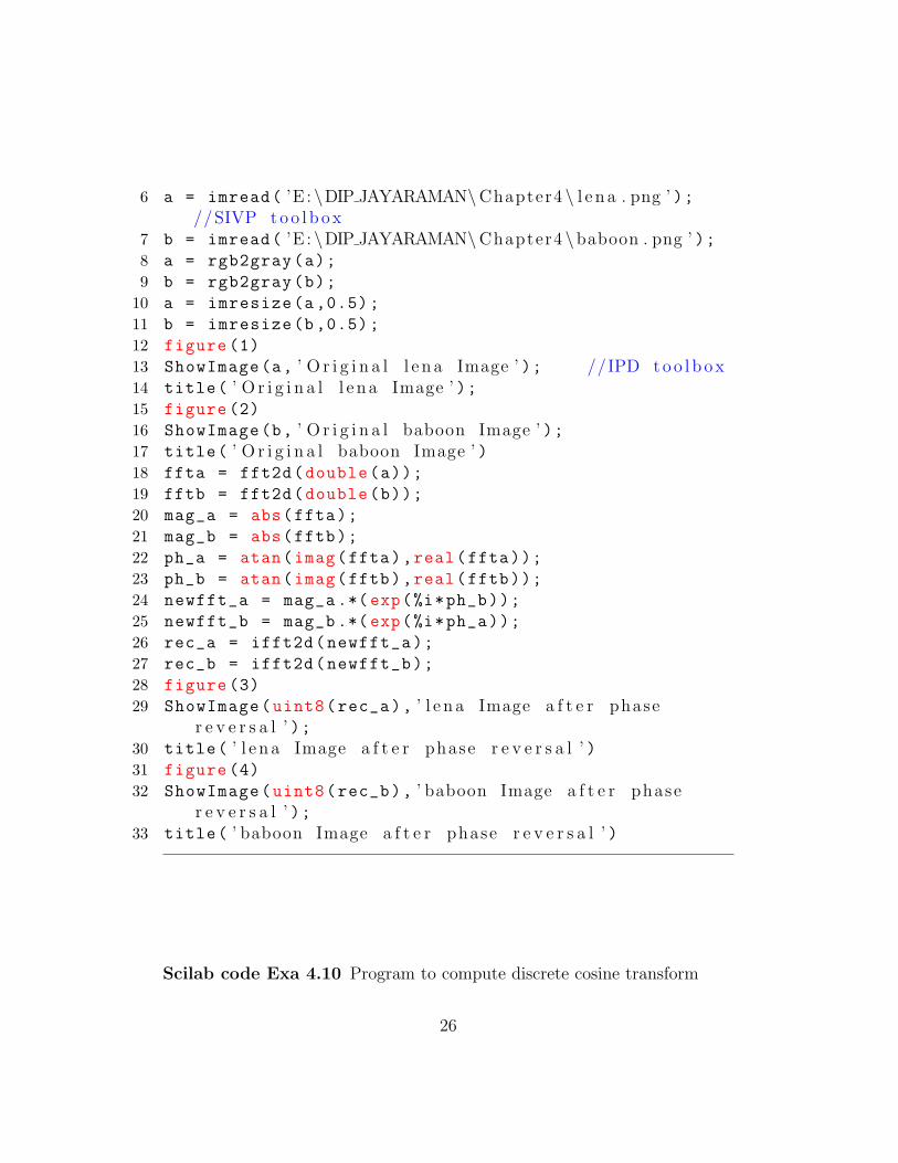
6 a = imread( ’E : \DIP JAYARAMAN\Chapter4 \ l e n a . png ’ );//SIVP t o o l b o x
7 b = imread( ’E : \DIP JAYARAMAN\Chapter4 \baboon . png ’ );8 a = rgb2gray(a);
9 b = rgb2gray(b);
10 a = imresize(a,0.5);
11 b = imresize(b,0.5);
12 figure (1)
13 ShowImage(a, ’ O r i g i n a l l e n a Image ’ ); //IPD t o o l b o x14 title( ’ O r i g i n a l l e n a Image ’ );15 figure (2)
16 ShowImage(b, ’ O r i g i n a l baboon Image ’ );17 title( ’ O r i g i n a l baboon Image ’ )18 ffta = fft2d(double(a));
19 fftb = fft2d(double(b));
20 mag_a = abs(ffta);
21 mag_b = abs(fftb);
22 ph_a = atan(imag(ffta),real(ffta));
23 ph_b = atan(imag(fftb),real(fftb));
24 newfft_a = mag_a .*(exp(%i*ph_b));
25 newfft_b = mag_b .*(exp(%i*ph_a));
26 rec_a = ifft2d(newfft_a);
27 rec_b = ifft2d(newfft_b);
28 figure (3)
29 ShowImage(uint8(rec_a), ’ l e n a Image a f t e r phaser e v e r s a l ’ );
30 title( ’ l e n a Image a f t e r phase r e v e r s a l ’ )31 figure (4)
32 ShowImage(uint8(rec_b), ’ baboon Image a f t e r phaser e v e r s a l ’ );
33 title( ’ baboon Image a f t e r phase r e v e r s a l ’ )
Scilab code Exa 4.10 Program to compute discrete cosine transform
26
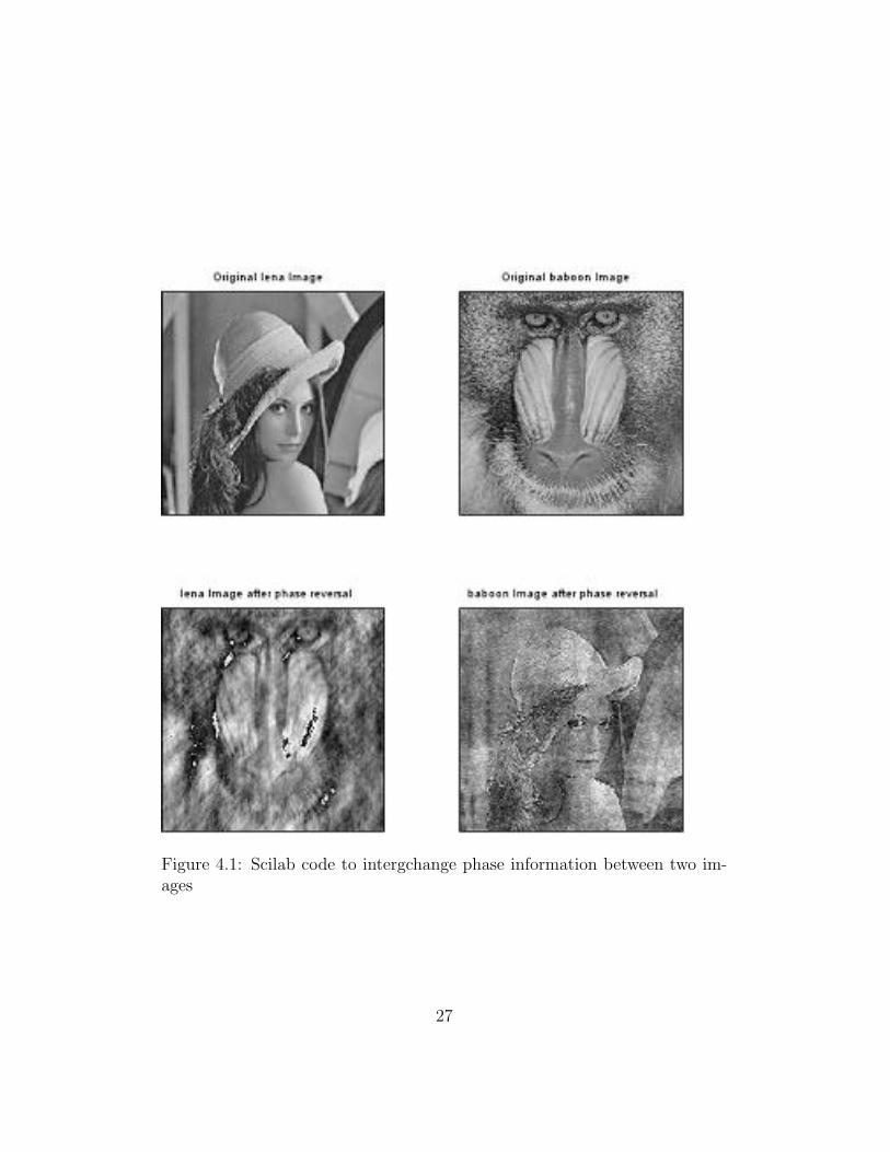
Figure 4.1: Scilab code to intergchange phase information between two im-ages
27
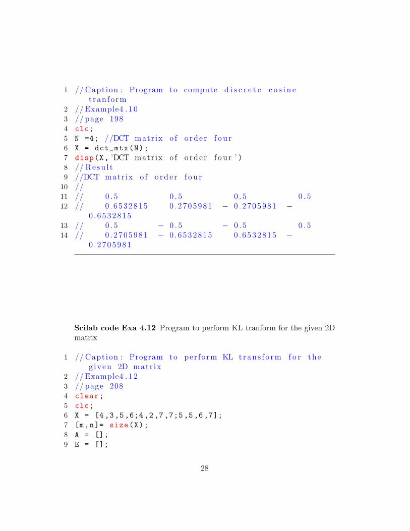
1 // Capt ion : Program to compute d i s c r e t e c o s i n et ran fo rm
2 // Example4 . 1 03 // page 1984 clc;
5 N =4; //DCT matr ix o f o r d e r f o u r6 X = dct_mtx(N);
7 disp(X, ’DCT matr ix o f o r d e r f o u r ’ )8 // R e s u l t9 //DCT matr ix o f o r d e r f o u r
10 //11 // 0 . 5 0 . 5 0 . 5 0 . 512 // 0 . 6 5 3 2 8 15 0 . 2 7 0 59 8 1 − 0 . 2 7 05 9 8 1 −
0 . 6 5 32 8 1 513 // 0 . 5 − 0 . 5 − 0 . 5 0 . 514 // 0 . 2 7 0 5 9 81 − 0 . 6 5 32 8 1 5 0 . 65 3 2 8 1 5 −
0 . 2 7 05 9 8 1
Scilab code Exa 4.12 Program to perform KL tranform for the given 2Dmatrix
1 // Capt ion : Program to per fo rm KL t r a n s f o r m f o r theg i v e n 2D matr ix
2 // Example4 . 1 23 // page 2084 clear;
5 clc;
6 X = [4,3,5,6;4,2,7,7;5,5,6,7];
7 [m,n]= size(X);
8 A = [];
9 E = [];
28

Figure 4.2: Program to compute discrete cosine transform
29
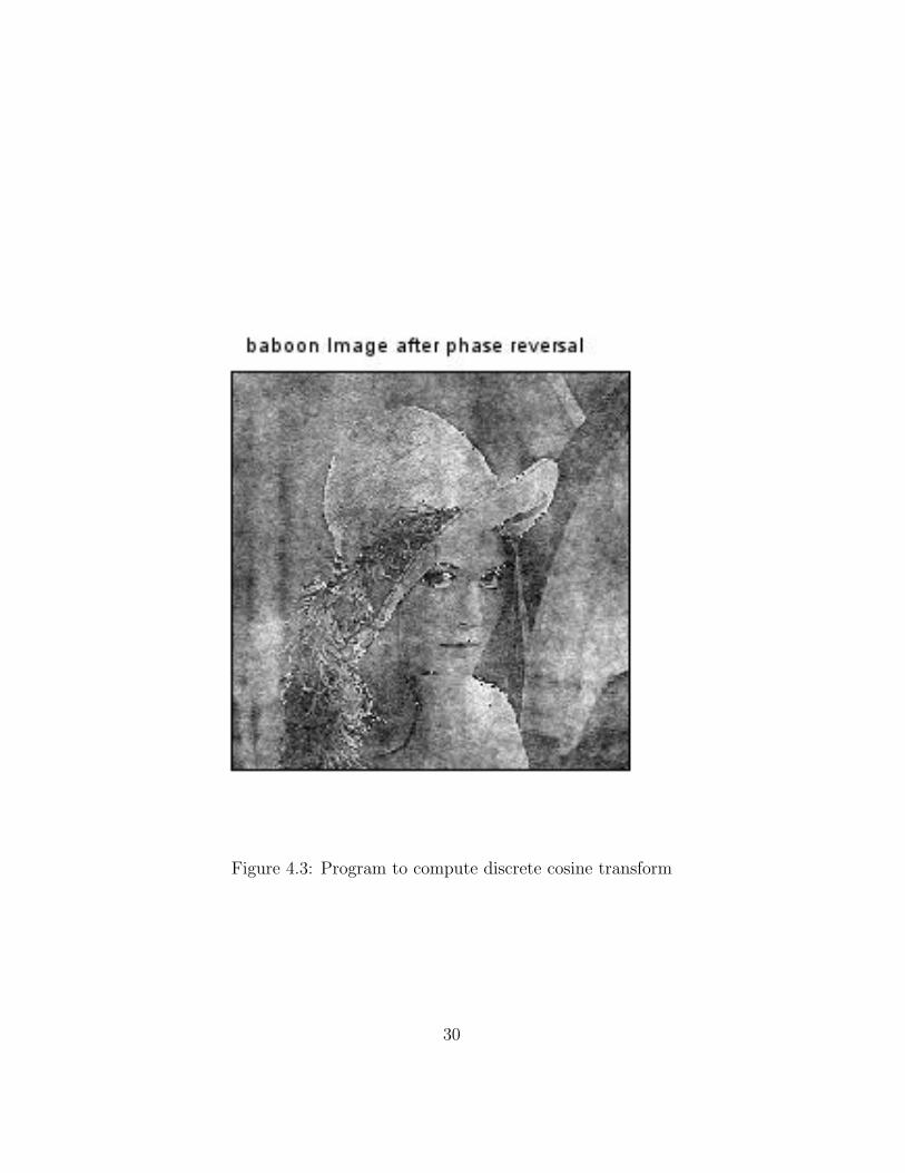
Figure 4.3: Program to compute discrete cosine transform
30
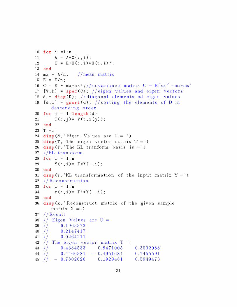
10 for i =1:n
11 A = A+X(:,i);
12 E = E+X(:,i)*X(:,i) ’;
13 end
14 mx = A/n; //mean matr ix15 E = E/n;
16 C = E - mx*mx ’; // c o v a r i a n c e matr ix C = E [ xx ’ ]−mx∗mx’17 [V,D] = spec(C); // e i g e n v a l u e s and e i g e n v e c t o r s18 d = diag(D); // d i a g o n a l e l e m e n t s od e i g e n v a l u e s19 [d,i] = gsort(d); // s o r t i n g the e l e m e n t s o f D i n
d e s c e n d i n g o r d e r20 for j = 1: length(d)
21 T(:,j)= V(:,i(j));
22 end
23 T =T’
24 disp(d, ’ E igen Values a r e U = ’ )25 disp(T, ’ The e i g e n v e c t o r matr ix T = ’ )26 disp(T, ’ The KL tran fo rm b a s i s i s = ’ )27 //KL t r a n s f o r m28 for i = 1:n
29 Y(:,i)= T*X(:,i);
30 end
31 disp(Y, ’KL t r a n s f o r m a t i o n o f the input matr ix Y = ’ )32 // R e c o n s t r u c t i o n33 for i = 1:n
34 x(:,i)= T’*Y(:,i);
35 end
36 disp(x, ’ R e c o n s t r u c t matr ix o f the g i v e n samplematr ix X = ’ )
37 // R e s u l t38 // Eigen Values a r e U =39 // 6 . 1 9 6 3 3 7240 // 0 . 2 1 4 7 4 1741 // 0 . 0 2 6 4 2 1142 // The e i g e n v e c t o r matr ix T =43 // 0 . 4 3 8 4 5 33 0 . 8 4 7 10 0 5 0 . 3 00 2 9 8 844 // 0 . 4 4 6 0 3 81 − 0 . 4 9 51 6 8 4 0 . 74 5 5 5 9 145 // − 0 . 7 8 02 6 2 0 0 . 19 2 9 4 8 1 0 . 5 9 4 9 4 7 3
31
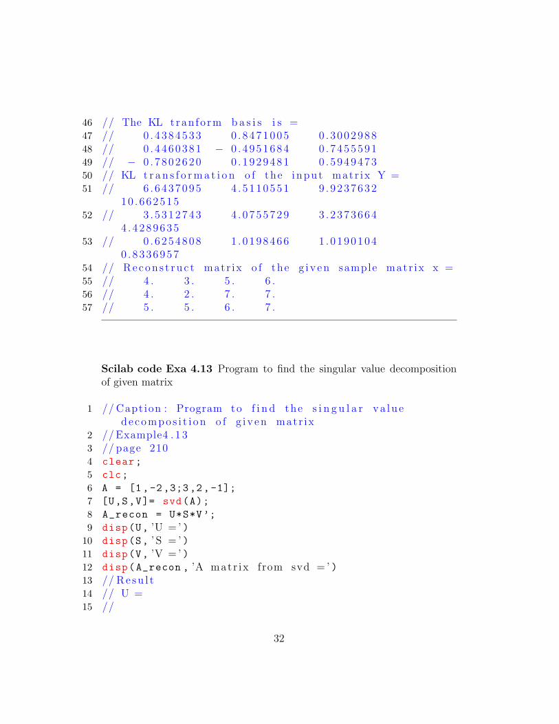
46 // The KL tran fo rm b a s i s i s =47 // 0 . 4 3 8 4 5 33 0 . 8 4 7 10 0 5 0 . 3 00 2 9 8 848 // 0 . 4 4 6 0 3 81 − 0 . 4 9 51 6 8 4 0 . 74 5 5 5 9 149 // − 0 . 7 8 02 6 2 0 0 . 19 2 9 4 8 1 0 . 5 9 4 9 4 7350 // KL t r a n s f o r m a t i o n o f the input matr ix Y =51 // 6 . 6 4 3 7 0 95 4 . 5 1 1 05 5 1 9 . 9 23 7 6 3 2
1 0 . 6 62 5 1 552 // 3 . 5 3 1 2 7 43 4 . 0 7 5 57 2 9 3 . 2 37 3 6 6 4
4 . 4 2 89 6 3 553 // 0 . 6 2 5 4 8 08 1 . 0 1 9 84 6 6 1 . 0 19 0 1 0 4
0 . 8 3 36 9 5 754 // R e c o n s t r u c t matr ix o f the g i v e n sample matr ix x =55 // 4 . 3 . 5 . 6 .56 // 4 . 2 . 7 . 7 .57 // 5 . 5 . 6 . 7 .
Scilab code Exa 4.13 Program to find the singular value decompositionof given matrix
1 // Capt ion : Program to f i n d the s i n g u l a r v a l u ed e c o m p o s i t i o n o f g i v e n matr ix
2 // Example4 . 1 33 // page 2104 clear;
5 clc;
6 A = [1,-2,3;3,2,-1];
7 [U,S,V]= svd(A);
8 A_recon = U*S*V’;
9 disp(U, ’U = ’ )10 disp(S, ’ S = ’ )11 disp(V, ’V = ’ )12 disp(A_recon , ’A matr ix from svd = ’ )13 // R e s u l t14 // U =15 //
32
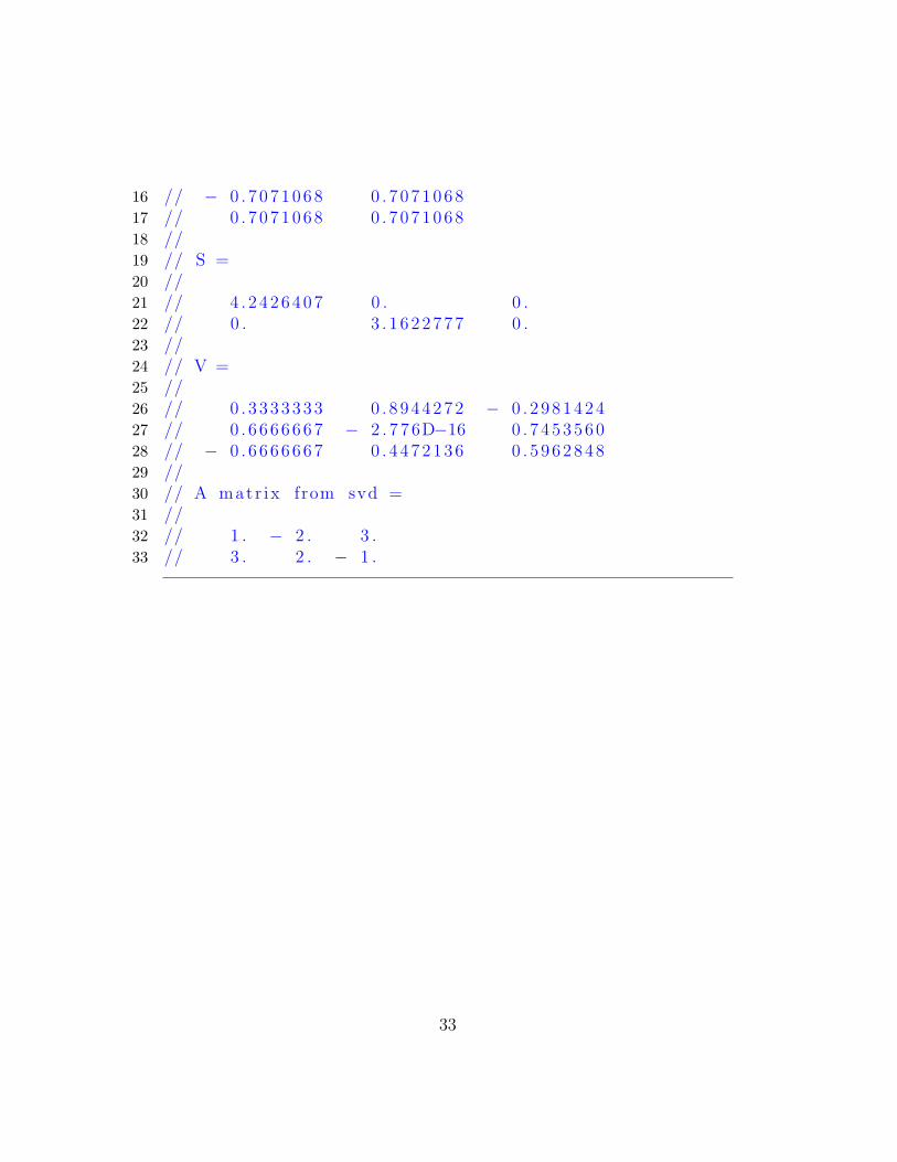
16 // − 0 . 7 0 71 0 6 8 0 . 70 7 1 0 6 817 // 0 . 7 0 7 1 0 68 0 . 7 0 7 10 6 818 //19 // S =20 //21 // 4 . 2 4 2 6 4 07 0 . 0 .22 // 0 . 3 . 1 6 2 2 77 7 0 .23 //24 // V =25 //26 // 0 . 3 3 3 3 3 33 0 . 8 9 4 42 7 2 − 0 . 2 9 81 4 2 427 // 0 . 6 6 6 6 6 67 − 2 . 7 7 6D−16 0 . 7 4 5 3 5 6 028 // − 0 . 6 6 66 6 6 7 0 . 44 7 2 1 3 6 0 . 5 9 6 2 8 4829 //30 // A matr ix from svd =31 //32 // 1 . − 2 . 3 .33 // 3 . 2 . − 1 .
33
Chapter 5
Image Enhancement
Scilab code Exa 5.5 Scilab code for brightness enhancement
1 // Capt ion : S c i l a b code f o r b r i g h t n e s s enhancement2 // Fig5 . 53 // page 2464 clc;
5 close;
6 // a = imread ( ’E : \DIP JAYARAMAN\Chapter5 \ p l a t e . GIF ’ ) ;//SIVP t o o l b o x
7 a = imread( ’E : \DIP JAYARAMAN\Chapter4 \baboon . png ’ );8 a = rgb2gray(a);
9 b = double(a)+50;
10 b = uint8(b);
11 figure (1)
12 ShowImage(a, ’ O r i g i n a l Image ’ );13 title( ’ O r i g i n a l Image ’ )14 figure (2)
15 ShowImage(b, ’ Enhanced Image ’ );16 title( ’ Enhanced Image ’ )
34

Figure 5.1: Scilab code for brightness enhancement
35
Scilab code Exa 5.7 Scilab code for brightness suppression
1 // Capt ion : S c i l a b code f o r b r i g h t n e s s s u p p r e s s i o n2 // Fig5 . 73 // page 2474 clc;
5 close;
6 a = imread( ’E : \DIP JAYARAMAN\Chapter4 \baboon . png ’ );7 a = rgb2gray(a);
8 b = double(a) -50;
9 b = uint8(b);
10 figure (1)
11 ShowImage(a, ’ O r i g i n a l Image ’ );12 title( ’ O r i g i n a l Image ’ )13 figure (2)
14 ShowImage(b, ’ B r i g h t n e s s Supr e s s ed Image ’ );15 title( ’ B r i g h t n e s s Supr e s s ed Image ’ )
Scilab code Exa 5.9 Scilab code for Contrast Manipulation
1 // Capt ion : S c i l a b code f o r Cont ra s t Man ipu la t i on2 // Fig5 . 93 // page 2484 clc;
5 close;
6 a = imread( ’E : \DIP JAYARAMAN\Chapter4 \ l e n a . png ’ );7 a = rgb2gray(a);
8 b = double(a)*0.5;
9 b = uint8(b)
10 c = double(b)*2;
36
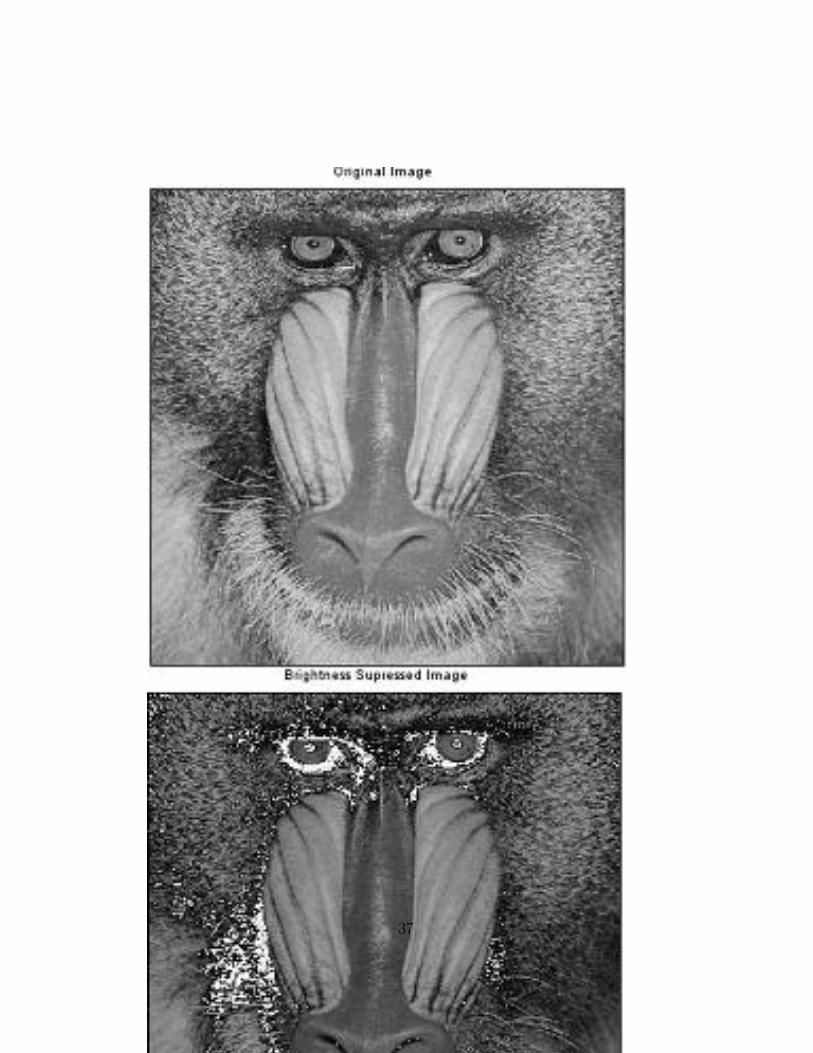
Figure 5.2: Scilab code for brightness suppression
37

11 c = uint8(c)
12 figure (1)
13 ShowImage(a, ’ O r i g i n a l Image ’ );14 title( ’ O r i g i n a l Image ’ )15 figure (2)
16 ShowImage(b, ’ Dec r ea s e i n Cont ra s t ’ );17 title( ’ Dec r ea s e i n Cont ra s t ’ )18 figure (3)
19 ShowImage(c, ’ I n c r e a s e i n Cont ra s t ’ );20 title( ’ I n c r e a s e i n Cont ra s t ’ )
Scilab code Exa 5.13 Scilab code to determine image negative
1 // Capt ion : S c i l a b code to de t e rmine image n e g a t i v e2 // Fig . 5 . 1 33 // page 2524 clc;
5 close;
6 a = imread( ’E : \DIP JAYARAMAN\Chapter5 \ l a b e l . j pg ’ );7 k = 255- double(a);
8 k = uint8(k);
9 imshow(a);
10 title( ’ O r i g i n a l onca Image ’ )11 imshow(k);
12 title( ’ Nega t i v e o f O r i g i n a l Image ’ )
Scilab code Exa 5.16 Scilab code that performs threshold operation
38

Figure 5.3: Scilab code for Contrast Manipulation
Figure 5.4: Scilab code to determine image negative
39
1 // Capt ion : S c i l a b code tha t pe r f o rms t h r e s h o l do p e r a t i o n
2 // Fig5 . 1 63 // page 2544 clc;
5 close;
6 a = imread( ’E : \ D i g i t a l I m a g e P r o c e s s i n g J a y a r a m a n \Chapter5 \ l e n a . png ’ );
7 a = rgb2gray(a);
8 [m n] = size(a);
9 t = input( ’ Enter the t h r e s h o l d parameter ’ );10 for i = 1:m
11 for j = 1:n
12 if(a(i,j)<t)
13 b(i,j)=0;
14 else
15 b(i,j)=255;
16 end
17 end
18 end
19 figure (1)
20 ShowImage(a, ’ O r i g i n a l Image ’ );21 title( ’ O r i g i n a l Image ’ )22 figure (2)
23 ShowImage(b, ’ Thre sho lded Image ’ );24 title( ’ Thre sho lded Image ’ )25 xlabel(sprintf( ’ Thre sho ld v a l u e i s %g ’ ,t))26 // R e s u l t27 // Enter the t h r e s h o l d parameter 140
Scilab code Exa 5.20 Program performs gray level slicing without back-ground
40

Figure 5.5: Scilab code that performs threshold operation
41

1 // Capt ion : Program per f o rms gray l e v e l s l i c i n gwi thout background
2 // Fig . 5 . 2 03 // page2564 clc;
5 x = imread( ’E : \ D i g i t a l I m a g e P r o c e s s i n g J a y a r a m a n \Chapter5 \ l e n a . png ’ );
6 x = rgb2gray(x);
7 y = double(x);
8 [m,n]= size(y);
9 L = max(max(x));
10 a = round(L/2);
11 b = L;
12 for i =1:m
13 for j =1:n
14 if(y(i,j)>=a & y(i,j)<=b)
15 z(i,j) = L;
16 else
17 z(i,j)=0;
18 end
19 end
20 end
21 z = uint8(z);
22 figure (1)
23 ShowImage(x, ’ O r i g i n a l Image ’ );24 title( ’ O r g i n a l Image ’ )25 figure (2)
26 ShowImage(z, ’ Gray Lev e l S l i c i n g ’ );27 title( ’ Gray Leve l S l i c i n g wi thout p r e s e r v i n g
background ’ )
42
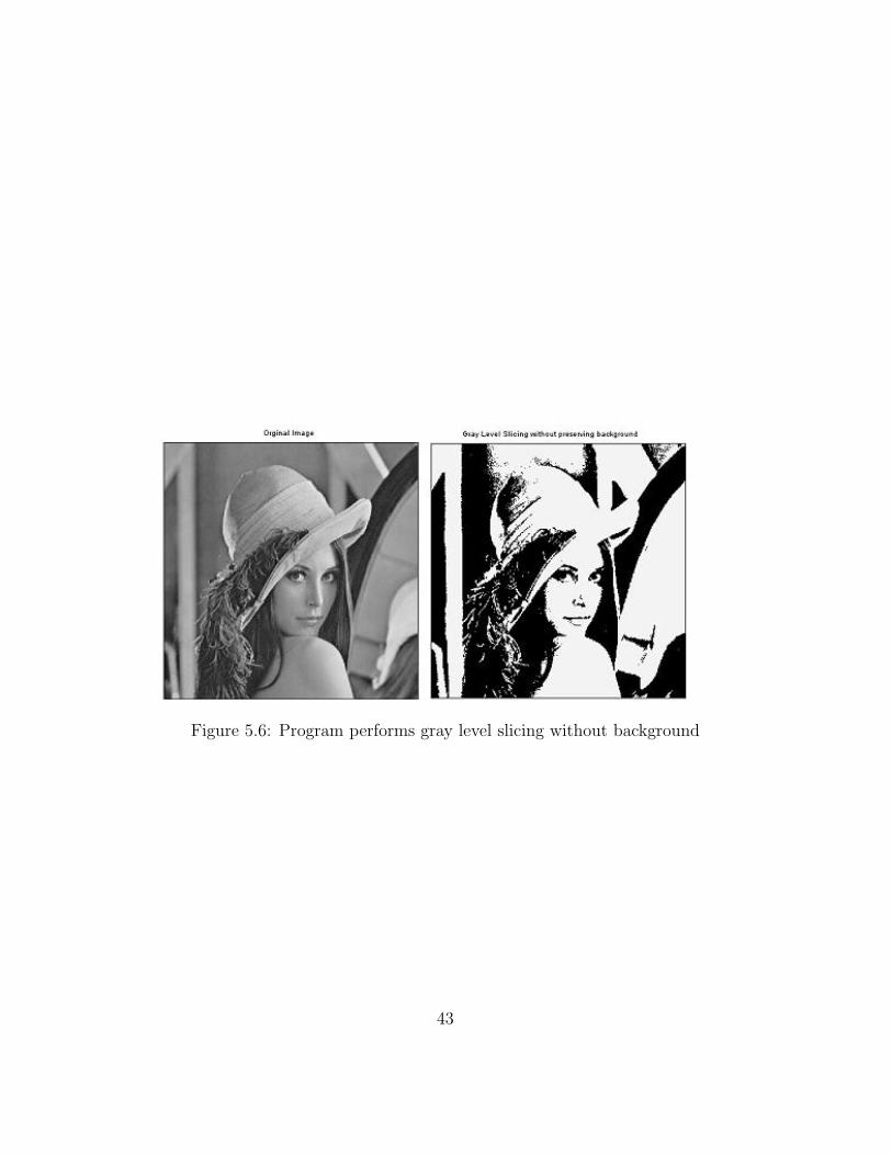
Figure 5.6: Program performs gray level slicing without background
43
Chapter 6
Image Restoration andDenoising
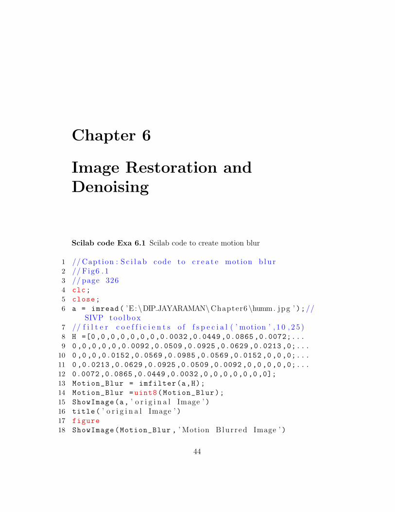
Scilab code Exa 6.1 Scilab code to create motion blur
1 // Capt ion : S c i l a b code to c r e a t e motion b l u r2 // Fig6 . 13 // page 3264 clc;
5 close;
6 a = imread( ’E : \DIP JAYARAMAN\Chapter6 \humm. jpg ’ );//SIVP t o o l b o x
7 // f i l t e r c o e f f i c i e n t s o f f s p e c i a l ( ’ motion ’ , 1 0 , 2 5 )8 H =[0 ,0 ,0 ,0 ,0 ,0 ,0 ,0.0032 ,0.0449 ,0.0865 ,0.0072;...
9 0 ,0 ,0 ,0 ,0 ,0.0092 ,0.0509 ,0.0925 ,0.0629 ,0.0213 ,0;...
10 0 ,0 ,0 ,0.0152 ,0.0569 ,0.0985 ,0.0569 ,0.0152 ,0 ,0 ,0;...
11 0 ,0.0213 ,0.0629 ,0.0925 ,0.0509 ,0.0092 ,0 ,0 ,0 ,0 ,0;...
12 0.0072 ,0.0865 ,0.0449 ,0.0032 ,0 ,0 ,0 ,0 ,0 ,0 ,0];
13 Motion_Blur = imfilter(a,H);
14 Motion_Blur =uint8(Motion_Blur);
15 ShowImage(a, ’ o r i g i n a l Image ’ )16 title( ’ o r i g i n a l Image ’ )17 figure
18 ShowImage(Motion_Blur , ’ Motion B lu r r ed Image ’ )
44

Figure 6.1: Scilab code to create motion blur
19 title( ’ 10 x25 Motion B lu r r ed Image ’ )
check Appendix AP 1 for dependency:
fft2d.sce
check Appendix AP 2 for dependency:
ifft2d.sce
Scilab code Exa 6.5 Scilab code performs inverse filtering
1 // Capt ion : S c i l a b code pe r f o rms i n v e r s e f i l t e r i n g2 // Degrade the image by means o f a known b l u r3 // Apply i n v e r s e f i l t e r to the b l u r r e d image and s e e
the r e s t o r e d image4 // Fig6 . 55 // page 3306 clc;
7 close;
45

8 x =imread( ’E : \DIP JAYARAMAN\Chapter6 \ f l o w e r 2 . jpg ’ );9 x=double(rgb2gray(x));
10 [M N]=size(x);
11 h = zeros(M,N);
12 for i = 1:11
13 for j = 1:11
14 h(i,j) = 1/121;
15 end
16 end
17 sigma = sqrt (4*10^( -7));
18 freqx = fft2d(x); // F o u r i e r t r a n s f o r m o f input image19 freqh = fft2d(h);// F o u r i e r t r a n s f o r m o f d e g r a d a t i o n20 y = real(ifft2d(freqh.*freqx));
21 freqy = fft2d(y);
22 powfreqx = freqx .^2/(M*N);
23 alpha = 0.5; // I n d i c a t e s i n v e r s e f i l t e r24 freqg = ((freqh.’) ’).*abs(powfreqx)./(abs(freqh .^2)
.*abs(powfreqx)+alpha*sigma ^2);
25 Resfreqx = freqg .* freqy;
26 Resa = real(ifft2d(Resfreqx));
27 x = uint8(x);
28 y = uint8(y);
29 Resa = uint8(Resa)
30 ShowImage(x, ’ O r i g i n a l Image ’ )31 title( ’ O r i g i n a l Image ’ )32 figure
33 ShowImage(y, ’ Degraded Image ’ )34 title( ’ Degraded Image ’ )35 figure
36 ShowImage(Resa , ’ Re s to r ed Image ’ )37 title( ’ Re s to r ed Image ’ )
check Appendix AP 1 for dependency:
fft2d.sce
check Appendix AP 2 for dependency:
46

Figure 6.2: Scilab code performs inverse filtering
47

ifft2d.sce
Scilab code Exa 6.7 Scilab code performs inverse filtering
1 // Capt ion : S c i l a b code pe r f o rms i n v e r s e f i l t e r i n g2 // Degrade the image by means o f a known b l u r and
whi te n o i s e3 //The image i s degraded as w e l l as c o r r u p t e d by
n o i s e4 // Apply i n v e r s e f i l t e r to r e s t o r e the image5 // Fig6 . 76 // page 3327 clc;
8 close;
9 x =imread( ’E : \DIP JAYARAMAN\Chapter6 \ f l o w e r 2 . jpg ’ );10 x=double(rgb2gray(x));
11 [M N]=size(x);
12 h = zeros(M,N);
13 for i = 1:11
14 for j = 1:11
15 h(i,j) = 1/121;
16 end
17 end
18 sigma = sqrt (4*10^( -7));
19 freqx = fft2d(x); // F o u r i e r t r a n s f o r m o f input image20 freqh = fft2d(h);// F o u r i e r t r a n s f o r m o f d e g r a d a t i o n21 y = real(ifft2d(freqh.*freqx))+10* rand(M,N, ’ normal ’ )
;
22 freqy = fft2d(y);
23 powfreqx = freqx .^2/(M*N);
24 alpha = 0.5; // I n d i c a t e s i n v e r s e f i l t e r25 freqg = ((freqh.’) ’).*abs(powfreqx)./(abs(freqh .^2)
.*abs(powfreqx)+alpha*sigma ^2);
26 Resfreqx = freqg .* freqy;
48
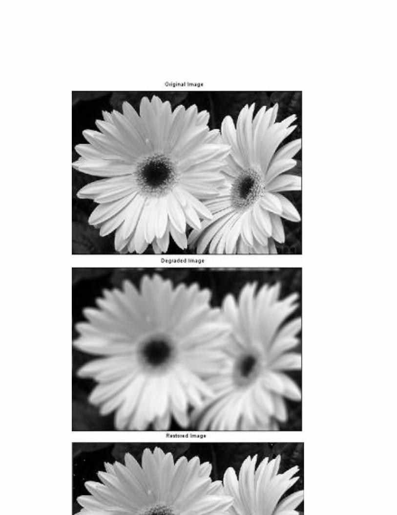
Figure 6.3: Scilab code performs inverse filtering
49

27 Resa = real(ifft2d(Resfreqx));
28 x = uint8(x);
29 y = uint8(y);
30 Resa = uint8(Resa)
31 ShowImage(x, ’ O r i g i n a l Image ’ )32 title( ’ O r i g i n a l Image ’ )33 figure
34 ShowImage(y, ’ Degraded+n o i s e Image ’ )35 title( ’ Degraded+n o i s e Image ’ )36 figure
37 ShowImage(Resa , ’ Re s to r ed Image ’ )38 title( ’ Re s to r ed Image ’ )
check Appendix AP 1 for dependency:
fft2d.sce
check Appendix AP 2 for dependency:
ifft2d.sce
Scilab code Exa 6.9 Scilab code performs Pseudo inverse filtering
1 // Capt ion : S c i l a b code pe r f o rms Pseudo i n v e r s ef i l t e r i n g
2 // Degrade the image by means o f a known b l u r andwhi te n o i s e
3 //The image i s degraded as w e l l as c o r r u p t e d byn o i s e
4 // Apply Pseudo i n v e r s e f i l t e r to r e s t o r e the image5 // Fig6 . 96 // page 3337 clc;
8 close;
9 x =imread( ’E : \DIP JAYARAMAN\Chapter6 \ f l o w e r 2 . jpg ’ );
50
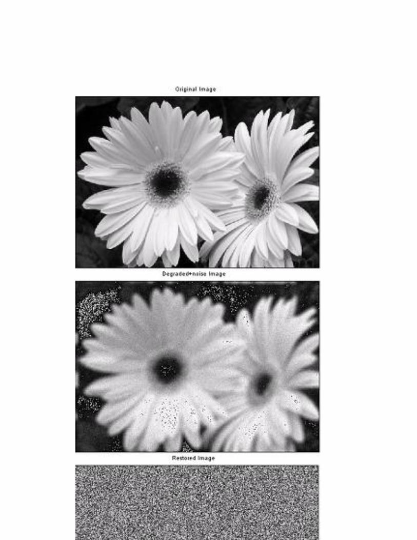
Figure 6.4: Scilab code performs inverse filtering
51

10 x=double(rgb2gray(x));
11 [M N]=size(x);
12 h = zeros(M,N);
13 for i = 1:11
14 for j = 1:11
15 h(i,j) = 1/121;
16 end
17 end
18 mask_b = ones (11 ,11) /121;
19 [m1 ,n1] = size(mask_b);
20 Thr_Freq = 0.2;
21 freqx = fft2d(x); // F o u r i e r t r a n s f o r m o f input image22 freqh = fft2d(h);// F o u r i e r t r a n s f o r m o f d e g r a d a t i o n23 y = real(ifft2d(freqh.*freqx))+25* rand(M,N, ’ normal ’ )
;
24 freqy = fft2d(y);
25 psf=zeros(M,N);
26 psf(M/2+1-(m1 -1) /2:M/2+1+(m1 -1)/2,N/2+1 -(n1 -1) /2:N
/2+1+(n1 -1)/2) = mask_b;
27 psf = fftshift(psf);
28 freq_res = fft2d(psf);
29 Inv_filt = freq_res ./(( abs(freq_res)).^2+ Thr_Freq);
30 z = real(ifft2d(freqy.* Inv_filt));
31 x = uint8(x);
32 y = uint8(y);
33 z = uint8(z)
34 ShowImage(x, ’ O r i g i n a l Image ’ )35 title( ’ O r i g i n a l Image ’ )36 figure
37 ShowImage(y, ’ Degraded+n o i s e Image ’ )38 title( ’ Degraded+n o i s e Image ’ )39 figure
40 ShowImage(z, ’ Re s to r ed Image ’ )41 title( ’ Re s to r ed Image ’ )
check Appendix AP 1 for dependency:
52

Figure 6.5: Scilab code performs Pseudo inverse filtering
53
fft2d.sce
check Appendix AP 2 for dependency:
ifft2d.sce
Scilab code Exa 6.13 Scilab code to perform wiener filtering of the cor-rupted image
1 // Capt ion : S c i l a b code to per fo rm wiene r f i l t e r i n go f the c o r r u p t e d image
2 // Fig6 . 1 33 // Page 3394 close;
5 clc;
6 x = imread( ’E : \DIP JAYARAMAN\Chapter6 \ f l o w e r 2 . jpg ’ );//SIVP t o o l b o x
7 x=double(rgb2gray(x));
8 sigma = 50;
9 Gamma = 1;
10 alpha = 1; // I t i n d i c a t e s Wiener f i l t e r11 [M N]=size(x);
12 h = zeros(M,N);
13 for i = 1:5
14 for j = 1:5
15 h(i,j) = 1/25;
16 end
17 end
18 Freqa = fft2d(x);
19 Freqh = fft2d(h);
20 y = real(ifft2d(Freqh.*Freqa)) // image d e g r a d a t i o n21 y = y+25* rand(M,N,” normal ”); // Adding random n o i s e
with normal d i s t r i b u t i o n22 Freqy = fft2d(y);
23 Powy = abs(Freqy).^2/(M*N);
24 sFreqh = Freqh .*( abs(Freqh) >0)+1/ Gamma*(abs(Freqh)
==0);
54
25 iFreqh = 1/ sFreqh;
26 iFreqh = iFreqh ’.*( abs(Freqh)*Gamma >1)+Gamma*abs(
sFreqh)*iFreqh *(abs(sFreqh)*Gamma <=1);
27 iFreqh = iFreqh /(max(max(abs(iFreqh))));
28 Powy = Powy .*(Powy >sigma ^2)+sigma ^2*(Powy <= sigma ^2);
29 Freqg = iFreqh .*(Powy -sigma ^2) ./(Powy -(1-alpha)*
sigma ^2);
30 ResFreqa = Freqg .* Freqy;
31 Resa = real(ifft2d(ResFreqa));
32 x = uint8(x);
33 y = uint8(y);
34 Resa = uint8(Resa);
35 ShowImage(x, ’ O r i g i n a l Image ’ )36 title( ’ O r i g i n a l Image ’ )37 figure
38 ShowImage(y, ’ Degraded Image ’ )39 title( ’ Degraded Image ’ )40 figure
41 ShowImage(Resa , ’ Re s to r ed Image ’ )42 title( ’ Re s to r ed Image ’ )
Scilab code Exa 6.18 Scilab code to Perform Average Filtering operation
1 // Capt ion : S c i l a b code to Perform Average F i l t e r i n go p e r a t i o n
2 // Fig6 . 1 83 // page 3494 clc;
5 close;
6 a= imread( ’E : \DIP JAYARAMAN\Chapter6 \ l enna . jpg ’ );//SIVP t o o l b o x
7 a=imnoise(a, ’ s a l t & pepper ’ , 0.2); //Add s a l t&peppern o i s e t o t h e image
55

Figure 6.6: Scilab code to perform wiener filtering of the corrupted image
56
8 a=double(a);
9 [m n]=size(a);
10 N=input( ’ e n t e r the window s i z e= ’ ); //The window s i z ecan be 3x3 , 5 x 5 e t c
11 Start=(N+1)/2;
12 Out_Imag=a;
13 for i=Start:(m-Start +1)
14 for j=Start:(n-Start +1)
15 limit=(N-1)/2;
16 Sum =0;
17 for k=-limit:limit ,
18 for l=-limit:limit ,
19 Sum=Sum+a(i+k,j+l);
20 end
21 end
22 Out_Imag(i,j)=Sum/(N*N);
23 end
24 end
25 a = uint8(a);
26 Out_Imag = uint8(Out_Imag);
27 ShowImage(a, ’ o r i g i n a l Image ’ )28 title( ’ Noisy Image ’ )29 figure
30 ShowImage(Out_Imag , ’ a v e r ag e f i l t e r e d Image ’ )31 title( ’ 5 x5 ave rage f i l t e r e d Image ’ );
Scilab code Exa 6.21 Scilab code to Perform median filtering
1 // Capt ion : S c i l a b code to Perform median f i l t e r i n g2 // Fig6 . 2 13 // page 3524 clc;
5 close;
57

Figure 6.7: Scilab code to Perform Average Filtering operation
6 c = imread( ’E : \DIP JAYARAMAN\Chapter6 \cameraman . jpg ’);//SIVP t o o l b o x
7 N = input( ’ Enter the window s i z e ’ );8 a = double(imnoise(c, ’ s a l t & pepper ’ ,0.2));9 [m,n] = size(a);
10 b = a;
11 if(modulo(N,2) ==1)
12 Start = (N+1)/2;
13 End = Start;
14 limit1 = (N-1) /2;
15 limit2 = limit1;
16 else
17 Start = N/2;
18 End = Start +1;
19 limit1 = (N/2) -1;
20 limit2 = limit1 +1;
21 end
22 for i = Start:(m-End+1)
23 for j = Start:(n-End+1)
24 I =1;
25 for k = -limit1:limit2
26 for l = -limit1:limit2
27 mat(I)= a(i+k,j+1)
28 I = I+1;
29 end
58
30 end
31 mat = gsort(mat);
32 if(modulo(N,2) ==1)
33 b(i,j) = (mat (((N^2)+1) /2));
34 else
35 b(i,j) = (mat((N^2)/2)+mat(((N^2) /2)+1))/2;
36 end
37 end
38 end
39 a = uint8(a);
40 b = uint8(b);
41 figure
42 ShowImage(c, ’ O r i g i n a l Image ’ )43 title( ’ O r i g i n a l Image ’ )44 figure
45 ShowImage(a, ’ n o i s y image ’ )46 title( ’ n o i s y image ’ )47 figure
48 ShowImage(b, ’ Median F i l t e r e d Image ’ )49 title( ’ 5 x5 Median F i l t e r e d Image ’ )
check Appendix AP 3 for dependency:
Func_medianall.sci
Scilab code Exa 6.23 Scilab code to Perform median filtering of colourimage
1 // Capt ion : S c i l a b code to Perform median f i l t e r i n g o fc o l o u r image
2 // Fig6 . 2 3 ( a )3 // page 3534 clc;
5 close;
59

Figure 6.8: Scilab code to Perform median filtering
6 a=imread( ’E : \DIP JAYARAMAN\Chapter6 \ peppe r s . png ’ );//SIVP t o o l b o x
7 N=input( ’ e n t e r the window s i z e ’ );8 b=imresize(a ,[256 ,256]);
9 b=imnoise(b, ’ s a l t & pepper ’ ,.1);10 [m n]=size(b);
11 R=b(:,:,1);
12 G=b(:,:,2);
13 B=b(:,:,3);
14 Out_R=Func_medianall(R,N);// Apply ing Median f i l t e rto R p lane
15 Out_G=Func_medianall(G,N);// Apply ing Median f i l t e rto G p lane
16 Out_B=Func_medianall(B,N);// Apply ing Median f i l t e rto B p lane
17 Out_Image (:,:,1)=Out_R;
18 Out_Image (:,:,2)=Out_G;
19 Out_Image (:,:,3)=Out_B;
60
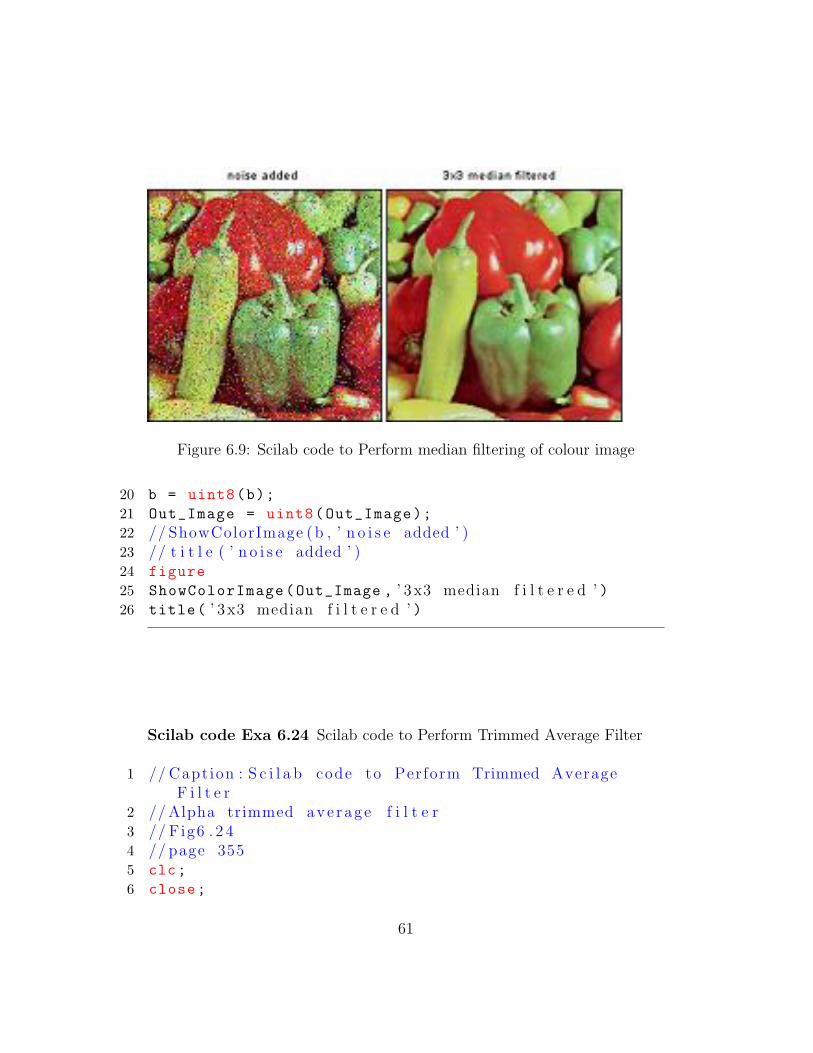
Figure 6.9: Scilab code to Perform median filtering of colour image
20 b = uint8(b);
21 Out_Image = uint8(Out_Image);
22 // ShowColorImage ( b , ’ n o i s e added ’ )23 // t i t l e ( ’ n o i s e added ’ )24 figure
25 ShowColorImage(Out_Image , ’ 3 x3 median f i l t e r e d ’ )26 title( ’ 3 x3 median f i l t e r e d ’ )
Scilab code Exa 6.24 Scilab code to Perform Trimmed Average Filter
1 // Capt ion : S c i l a b code to Perform Trimmed AverageF i l t e r
2 // Alpha trimmed ave rage f i l t e r3 // Fig6 . 2 44 // page 3555 clc;
6 close;
61
7 c = imread( ’E : \DIP JAYARAMAN\Chapter6 \ l enna . jpg ’ );//SIVP t o o l b o x
8 s = 1; // s d e n o t e s the number o f v a l u e s to be l e f ti n the end
9 r = 1;
10 N = 9; // 3 x3 window11 a = double(imnoise(c, ’ g a u s s i a n ’ ));12 [m,n] = size(a);
13 b = zeros(m,n);
14 for i= 2:m-1
15 for j = 2:n-1
16 mat = [a(i,j),a(i,j-1),a(i,j+1),a(i-1,j),a(i
+1,j),a(i-1,j-1) ,...
17 a(i-1,j+1),a(i-1,j+1),a(i+1,j+1)];
18 sorted_mat = gsort(mat);
19 Sum =0;
20 for k=r+s:(N-s)
21 Sum = Sum+mat(k);
22 end
23 b(i,j)= Sum/(N-r-s);
24 end
25 end
26 a = uint8(a);
27 b = uint8(b);
28 // f i g u r e29 // imshow ( c )30 // t i t l e ( ’ O r i g i n a l Image ’ )31 figure
32 ShowImage(a, ’ n o i s y image ’ )33 title( ’ n o i s y image ’ )34 figure
35 ShowImage(b, ’ Trimmed Average F i l t e r e d Image ’ )36 title( ’ Trimmed Average F i l t e r e d Image ’ )
62
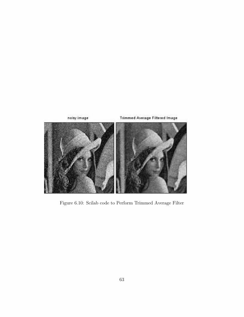
Figure 6.10: Scilab code to Perform Trimmed Average Filter
63

Chapter 7
Image Segmentation
Scilab code Exa 7.23 Scilab code for Differentiation of Gaussian function
1 // Capt ion : S c i l a b code f o r D i f f e r e n t i a t i o n o fGauss ian f u n c t i o n
2 // Fig7 . 2 33 // page3884 clc;
5 close;
6 sigma=input( ’ Enter the v a l u e o f s igma : ’ )7 i= -10:.1:10;
8 j= -10:.1:10;
9 r=sqrt(i.*i+j.*j);
10 y=(1/( sigma ^2))*(((r.*r)/sigma ^2) -1).*exp(-r.*r/2*
sigma ^2);
11 plot(i,y)
12 legend(sprintf( ’ The s igma v a l u e i s %g ’ ,sigma))13 xtitle( ’ D i f f e r e n t i a t i o n o f Gauss ian f u n c t i o n ’ )
64
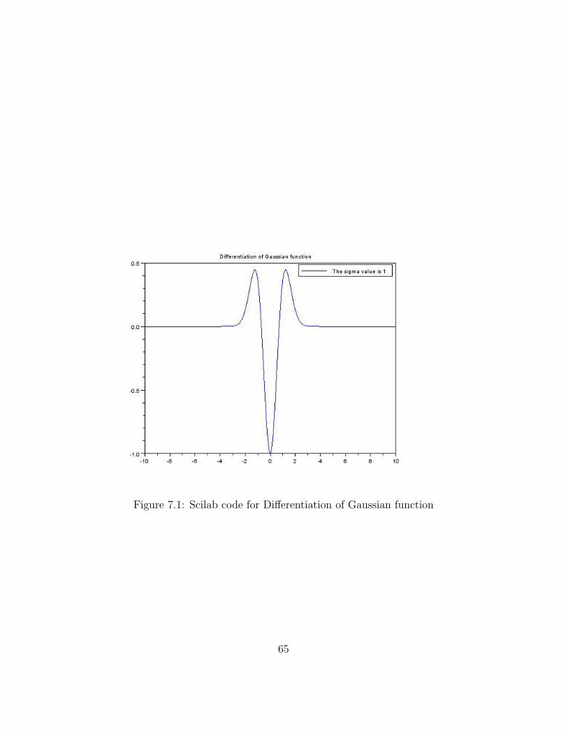
Figure 7.1: Scilab code for Differentiation of Gaussian function
65

Figure 7.2: Scilab code for Differentiation of Gaussian function
66
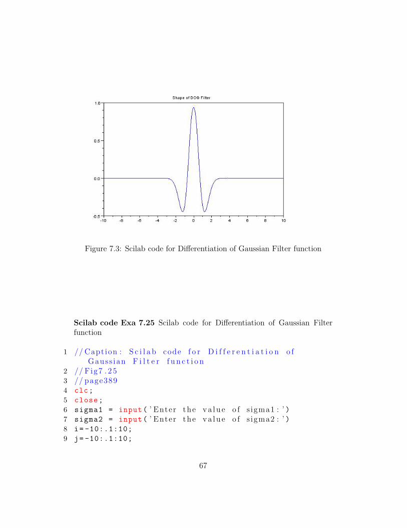
Figure 7.3: Scilab code for Differentiation of Gaussian Filter function
Scilab code Exa 7.25 Scilab code for Differentiation of Gaussian Filterfunction
1 // Capt ion : S c i l a b code f o r D i f f e r e n t i a t i o n o fGauss ian F i l t e r f u n c t i o n
2 // Fig7 . 2 53 // page3894 clc;
5 close;
6 sigma1 = input( ’ Enter the v a l u e o f s igma1 : ’ )7 sigma2 = input( ’ Enter the v a l u e o f s igma2 : ’ )8 i= -10:.1:10;
9 j= -10:.1:10;
67
Figure 7.4: Scilab code for Differentiation of Gaussian Filter function
10 r=sqrt(i.*i+j.*j);
11 y1 = (1/( sigma1 ^2))*(((r.*r)/sigma1 ^2) -1).*exp(-r.*r
/2* sigma1 ^2);
12 y2 = (1/( sigma2 ^2))*(((r.*r)/sigma2 ^2) -1).*exp(-r.*r
/2* sigma2 ^2);
13 y = y1 -y2;
14 plot(i,y)
15 xtitle( ’ Shape o f DOG F i l t e r ’ )16 // R e s u l t17 // Enter the v a l u e o f s igma1 : 418 // Enter the v a l u e o f s igma2 : 119 //
68
Scilab code Exa 7.27 Scilab code for Edge Detection using Different Edgedetectors
1 // Capt ion : S c i l a b code f o r Edge D e t e c t i o n u s i n gD i f f e r e n t Edge d e t e c t o r s
2 // [ 1 ] . Sobe l [ 2 ] . P r e w i t t [ 3 ] . Log [ 4 ] . Canny3 // Fig7 . 2 74 // page3895 close;
6 clc;
7 a = imread( ’E : \DIP JAYARAMAN\Chapter7 \ s a i l i n g . jpg ’ );8 a = rgb2gray(a);
9 c = edge(a, ’ s o b e l ’ );10 d = edge(a, ’ p r e w i t t ’ );11 e = edge(a, ’ l o g ’ );12 f = edge(a, ’ canny ’ );13 ShowImage(a, ’ O r i g i n a l Image ’ )14 title( ’ O r i g i n a l Image ’ )15 figure
16 ShowImage(c, ’ Sobe l ’ )17 title( ’ Sobe l ’ )18 figure
19 ShowImage(d, ’ P r e w i t t ’ )20 title( ’ P r e w i t t ’ )21 figure
22 ShowImage(e, ’ Log ’ )23 title( ’ Log ’ )24 figure
25 ShowImage(f, ’ Canny ’ )26 title( ’ Canny ’ )
69
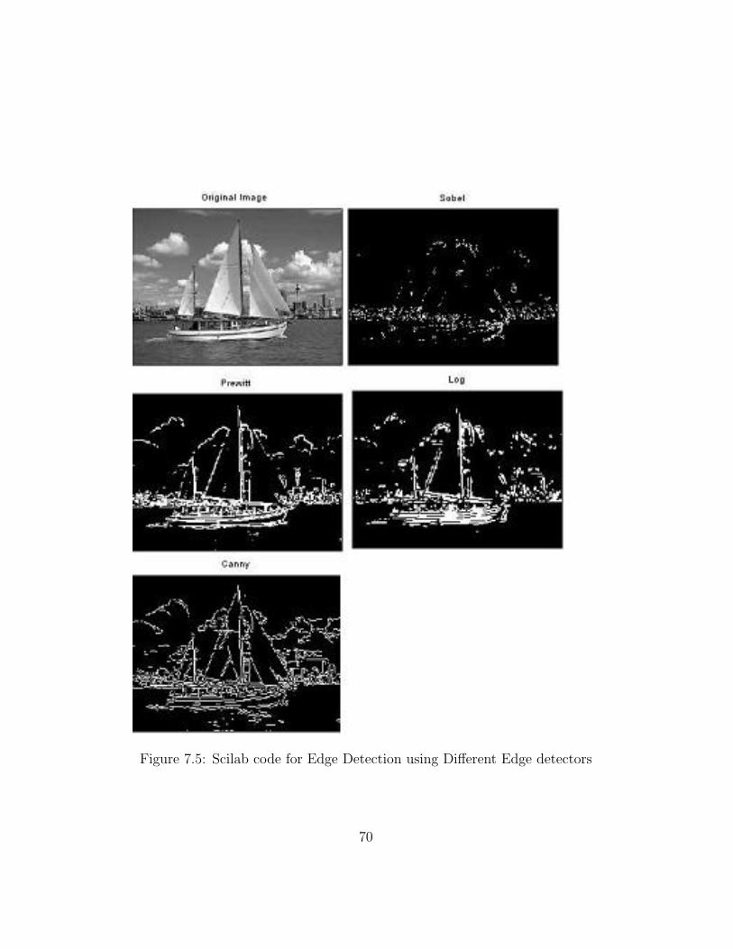
Figure 7.5: Scilab code for Edge Detection using Different Edge detectors
70
Scilab code Exa 7.30 Scilab code to perform watershed transform
1 // Capt ion : S c i l a b code to per fo rm wate r shedt r a n s f o r m
2 // Fig7 . 3 03 // Page3964 clc;
5 close;
6 b = imread( ’E : \DIP JAYARAMAN\Chapter7 \ t e a s e t . png ’ );7 a = rgb2gray(b);
8 global EDGE_SOBEL;
9 Gradient = EdgeFilter(a, EDGE_SOBEL);
10 Threshold1 = CalculateOtsuThreshold(Gradient); //de t e rmine a t h r e s h o l d
11 EdgeImage = ~SegmentByThreshold(Gradient ,Threshold1)
;
12 DistanceImage = DistanceTransform(EdgeImage);
13 Threshold2 = CalculateOtsuThreshold(DistanceImage)
// de t e rmine a t h r e s h o l d14 ThresholdImage = SegmentByThreshold(DistanceImage ,
Threshold2);
15 MarkerImage = SearchBlobs(ThresholdImage);
16 SegmentedImage = Watershed(Gradient ,MarkerImage);
17 figure
18 ShowColorImage(b, ’ t e a s e t ’ )19 title( ’ t e a s e t . png ’ )20 figure
21 ColorMapLength = length(unique(SegmentedImage));
22 ShowImage(SegmentedImage , ’ R e s u l t o f WatershedTransform ’ ,jetcolormap(ColorMapLength));
71
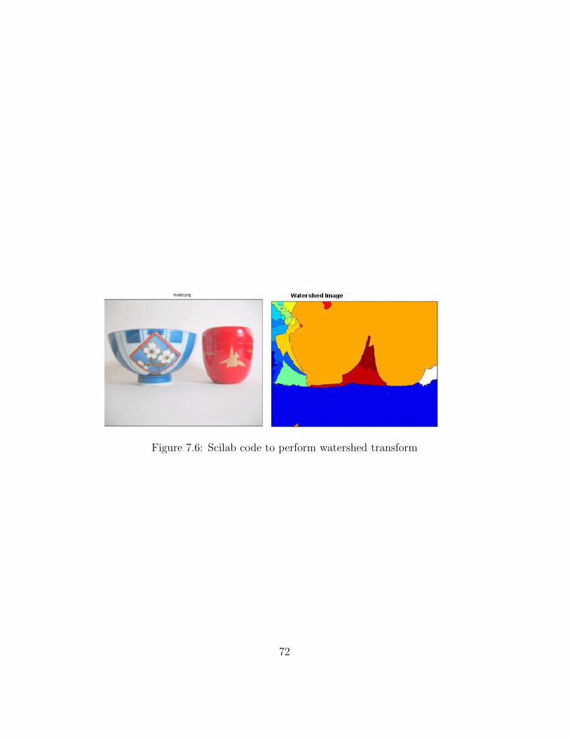
Figure 7.6: Scilab code to perform watershed transform
72
Chapter 8
Object Recognition
Scilab code Exa 8.4 To verify the given matrix is a covaraince matrix
1 // Capt ion : To v e r i f y the g i v e n matr ix i s ac o v a r a i n c e matr ix
2 // Problem 43 // page4384 close;
5 clear all;
6 clc;
7 K = [37 , -15; -15 ,37];
8 evals = spec(K);
9 evals = gsort(evals);
10 disp(evals , ’ E igen Values a r e = ’ )11 if (evals ==abs(evals)) then
12 disp( ’ Both the e i g e n v a l u e s a r e non−n e g a t i v e andthe g i v e n matr ix i s a c o v a r i a n c e matr ix ’ );
13 else
14 disp( ’ non−c o v a r i a n c e matr ix ’ )15 end
Scilab code Exa 8.5 To compute the covariance of the given 2D data
73
1 // Capt ion : To compute the c o v a r i a n c e o f the g i v e n 2Ddata
2 // Problem 53 // page4394 close;
5 clear all;
6 clc;
7 X1 = [2,1]’;
8 X2 = [3,2]’;
9 X3 = [2,3]’;
10 X4 = [1,2]’;
11 X = [X1,X2,X3,X4];
12 disp(X, ’X= ’ );13 [M,N] = size(X); //M=rows , N = columns14 for i =1:N
15 m(i) = mean(X(:,i));
16 A(:,i) = X(:,i)-m(i);
17 end
18 m = m’;
19 disp(m, ’ mean = ’ );20 K = A’*A;
21 K = K/(M-1);
22 disp(K, ’ The Covara ince matix i s K = ’ )23 // R e s u l t24 //X=25 // 2 . 3 . 2 . 1 .26 // 1 . 2 . 3 . 2 .27 //mean =28 // 1 . 5 2 . 5 2 . 5 1 . 529 //30 //The Covara ince matix i s K =31 // 0 . 5 0 . 5 − 0 . 5 − 0 . 532 // 0 . 5 0 . 5 − 0 . 5 − 0 . 533 // − 0 . 5 − 0 . 5 0 . 5 0 . 534 // − 0 . 5 − 0 . 5 0 . 5 0 . 5
74

Scilab code Exa 8.9 Develop a perceptron AND function with bipolar in-puts and targets
1 // Capt ion : Develop a p e r c e p t r o n AND f u n c t i o n withb i p o l a r i n p u t s and t a r g e t s
2 // Problem 93 // page4414 close;
5 clear all;
6 clc;
7 X1 = [1,-1,1,-1]; //X1 and X2 a r e input v e c t o r s toAND f u n c t i o n
8 X2 = [1,1,-1,-1];
9 //b = [ 1 , 1 , 1 , 1 ] ; // B i a s i n g v e c t o r10 T = [1,-1,-1,-1]; // Target v e c t o r f o r AND f u n c t i o n11 W1 = 0; // Weights a r e i n i t i a l i z e d12 W2 = 0;
13 b = 0; // b i a s i n i t i a l i z e d14 alpha = 1; // l e a r n i n g r a t e15 for i = 1: length(X1)
16 Yin(i) = b+X1(i)*W1+X2(i)*W2;
17 if (Yin(i) >=1)
18 Y(i)=1;
19 elseif ((Yin(i) <1)&(Yin(i) >=-1))
20 Y(i)=0;
21 elseif(Yin(i) <-1)
22 Y(i)=-1;
23 end
24 disp(Yin(i), ’ Yin= ’ )25 disp(Y(i), ’Y= ’ )26 if(Y(i)~=T(i))
27 b = b+alpha*T(i);
28 W1 = W1+alpha*T(i)*X1(i);
29 W2 = W2+alpha*T(i)*X2(i);
75
30 disp(b, ’ b= ’ )31 disp(W1, ’W1= ’ )32 disp(W2, ’W2= ’ )33 end
34 end
35 disp( ’ F i n a l Weights a f t e r one i t e r a t i o n a r e ’ )36 disp(b, ’ B ia s Weigth b= ’ )37 disp(W1, ’W1= ’ )38 disp(W2, ’W2= ’ )
76

Chapter 9
Image Compression
Scilab code Exa 9.9 Program performs Block Truncation Coding BTC
1 // Capt ion : Program per f o rms Block Truncat i on Coding (BTC)
2 // Example 9 . 93 // page5124 close;
5 clear all;
6 clc;
7 x =
[65 ,75 ,80 ,70;72 ,75 ,82 ,68;84 ,72 ,62 ,65;66 ,68 ,72 ,80];
8 disp(x, ’ O r i g i n a l Block i s x = ’ )9 [m1 n1]=size(x);
10 blk=input( ’ Enter the b l o c k s i z e : ’ );11 for i = 1 : blk : m1
12 for j = 1 : blk : n1
13 y = x(i:i+(blk -1),j:j+(blk -1)) ;
14 m = mean(mean(y));
15 disp(m, ’ mean v a l u e i s m = ’ )16 sig=std2(y);
17 disp(sig , ’ Standard d e v i a t i o n o f the b l o c k i s= ’ )
77
18 b = y > m ; // the b i n a ry b l o c k19 disp(b, ’ B inary a l l o c a t i o n matr ix i s B= ’ )20 K = sum(sum(b));
21 disp(K, ’ number o f ones = ’ )22 if (K ~= blk^2 ) & ( K ~= 0)
23 ml = m-sig*sqrt(K/(( blk ^2)-K));
24 disp(ml, ’ The v a l u e o f a = ’ )25 mu = m+sig*sqrt (((blk ^2)-K)/K);
26 disp(mu, ’ The v a l u e o f b = ’ )27 x(i:i+(blk -1), j:j+(blk -1)) = b*mu
+(1- b)*ml;
28 end
29 end
30 end
31 disp(round(x), ’ R e c on s t r u c t e d Block i s x = ’ )32 // R e s u l t33 // O r i g i n a l Block i s x =34 //35 // 6 5 . 7 5 . 8 0 . 7 0 .36 // 7 2 . 7 5 . 8 2 . 6 8 .37 // 8 4 . 7 2 . 6 2 . 6 5 .38 // 6 6 . 6 8 . 7 2 . 8 0 .39 //40 // Enter the b l o c k s i z e : 441 //mean v a l u e i s m = 7 2 . 2 542 // Standard d e v i a t i o n o f the b l o c k i s = 6 . 6 2 8 2 2 2 543 // Binary a l l o c a t i o n matr ix i s B=44 //45 // F T T F46 // F T T F47 // T F F F48 // F F F T49 //50 // number o f ones = 651 //The v a l u e o f a = 6 7 . 1 1 5 8 0152 //The v a l u e o f b = 8 0 . 8 06 9 9 853 // R e c o n s t r u c t e d Block i s x =54 //
78

55 // 6 7 . 8 1 . 8 1 . 6 7 .56 // 6 7 . 8 1 . 8 1 . 6 7 .57 // 8 1 . 6 7 . 6 7 . 6 7 .58 // 6 7 . 6 7 . 6 7 . 8 1 .
Scilab code Exa 9.59 Program performs Block Truncation Coding
1 // Capt ion : Program per f o rms Block Truncat i on Coding (BTC) by c h o o s i n g d i f f e r e n t
2 // b l o c k s i z e s3 // Fig . 9 . 5 9 : MATLAB Example14 // page5145 close;
6 clc;
7 x =imread( ’E : \ D i g i t a l I m a g e P r o c e s s i n g J a y a r a m a n \Chapter9 \ l enna . jpg ’ ); //SIVP t o o l b o x
8 //x=i m r e s i z e ( x , [ 2 5 6 2 5 6 ] ) ;9 x1=x;
10 x=double(x);
11 [m1 n1]=size(x);
12 blk=input( ’ Enter the b l o c k s i z e : ’ );13 for i = 1 : blk : m1
14 for j = 1 : blk : n1
15 y = x(i:i+(blk -1),j:j+(blk -1)) ;
16 m = mean(mean(y));
17 sig=std2(y);
18 b = y > m ; // the b i n a r y b l o c k19 K = sum(sum(b));
20 if (K ~= blk^2 ) & ( K ~= 0)
21 ml = m-sig*sqrt(K/(( blk ^2)-K));
22 mu = m+sig*sqrt (((blk ^2)-K)/K);
23 x(i:i+(blk -1), j:j+(blk -1)) = b*mu
+(1- b)*ml;
24 end
25 end
79
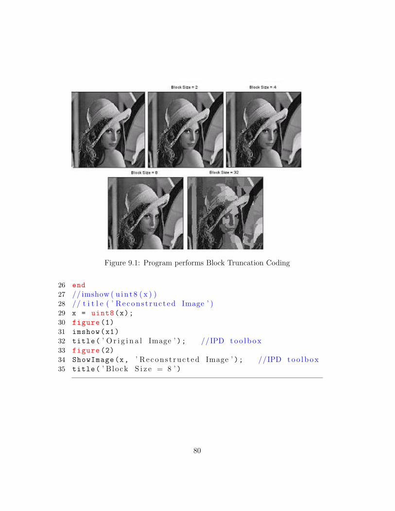
Figure 9.1: Program performs Block Truncation Coding
26 end
27 // imshow ( u i n t 8 ( x ) )28 // t i t l e ( ’ R e c o n s t r u c t e d Image ’ )29 x = uint8(x);
30 figure (1)
31 imshow(x1)
32 title( ’ O r i g i n a l Image ’ ); //IPD t o o l b o x33 figure (2)
34 ShowImage(x, ’ R e c on s t r u c t e d Image ’ ); //IPD t o o l b o x35 title( ’ Block S i z e = 8 ’ )
80
Chapter 10
Binary Image Processing
Scilab code Exa 10.17 Scilab Code for dilation and erosion process
1 // Capt ion : S c i l a b Code f o r d i l a t i o n and e r o s i o np r o c e s s
2 // Fig . 1 0 . 1 73 // Page5534 close;
5 clear all;
6 clc;
7 a = imread( ’E : \DIP JAYARAMAN\Chapter10 \morph1 . bmp ’ );//SIVP t o o l b o x
8 //b = [ 1 , 1 , 1 ; 1 , 1 , 1 ; 1 , 1 , 1 ] ;9 StructureElement = CreateStructureElement( ’ s qua r e ’ ,
3) ;
10 a1 = DilateImage(a,StructureElement);
11 a2 = ErodeImage(a,StructureElement);
12 // D i s p l a y i n g o r i g i n a l Image13 // imshow ( a )14 figure (1)
15 ShowImage(a, ’ O r i g i n a l Image ’ );16 // D i s p l a y i n g D i l a t e d Image17 // imshow ( a1 )18 figure (2)
81
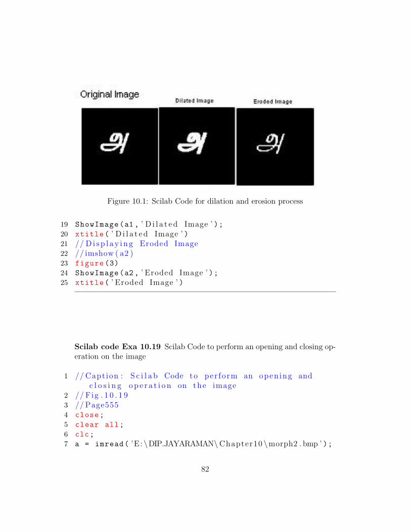
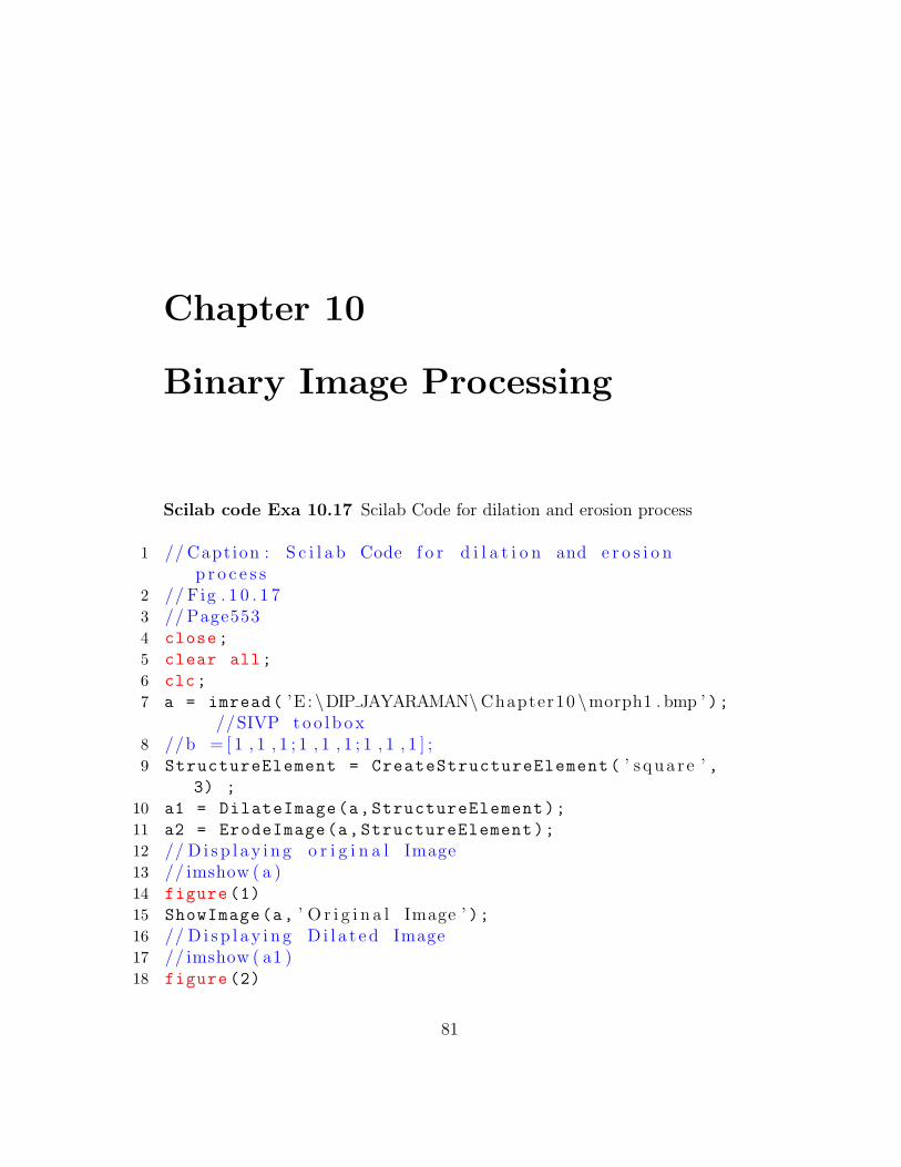
Figure 10.1: Scilab Code for dilation and erosion process
19 ShowImage(a1 , ’ D i l a t e d Image ’ );20 xtitle( ’ D i l a t e d Image ’ )21 // D i s p l a y i n g Eroded Image22 // imshow ( a2 )23 figure (3)
24 ShowImage(a2 , ’ Eroded Image ’ );25 xtitle( ’ Eroded Image ’ )
Scilab code Exa 10.19 Scilab Code to perform an opening and closing op-eration on the image
1 // Capt ion : S c i l a b Code to per fo rm an open ing andc l o s i n g o p e r a t i o n on the image
2 // Fig . 1 0 . 1 93 // Page5554 close;
5 clear all;
6 clc;
7 a = imread( ’E : \DIP JAYARAMAN\Chapter10 \morph2 . bmp ’ );
82

//SIVP t o o l b o x8 //b = [ 1 , 1 , 1 ; 1 , 1 , 1 ; 1 , 1 , 1 ] ;9 StructureElement = CreateStructureElement( ’ s qua r e ’ ,
3) ;
10 // Opening i s done by f i r s t a p p l y i n g e r o s i o n and thend i l a t i o n o p e r a t i o n s on image
11 b1 = ErodeImage(a,StructureElement);
12 b2 = DilateImage(b1,StructureElement);
13 // C l o s i n g i s done by f i r s t a p p l y i n g d i l a t i o n andthen e r o s i o n o p e r a t i o n on image
14 a1 = DilateImage(a,StructureElement);
15 a2 = ErodeImage(a1,StructureElement);
16 // D i s p l a y i n g o r i g i n a l Image17 figure (1)
18 ShowImage(a, ’ O r i g i n a l Image ’ );19 // D i s p l a y i n g Opened Image20 figure (2)
21 ShowImage(b2 , ’ Opened Image ’ );22 xtitle( ’ Opened Image ’ )23 // D i s p l a y i n g Closed Image24 figure (3)
25 ShowImage(a2 , ’ C lo sed Image ’ );26 xtitle( ’ C lo sed Image ’ )
83
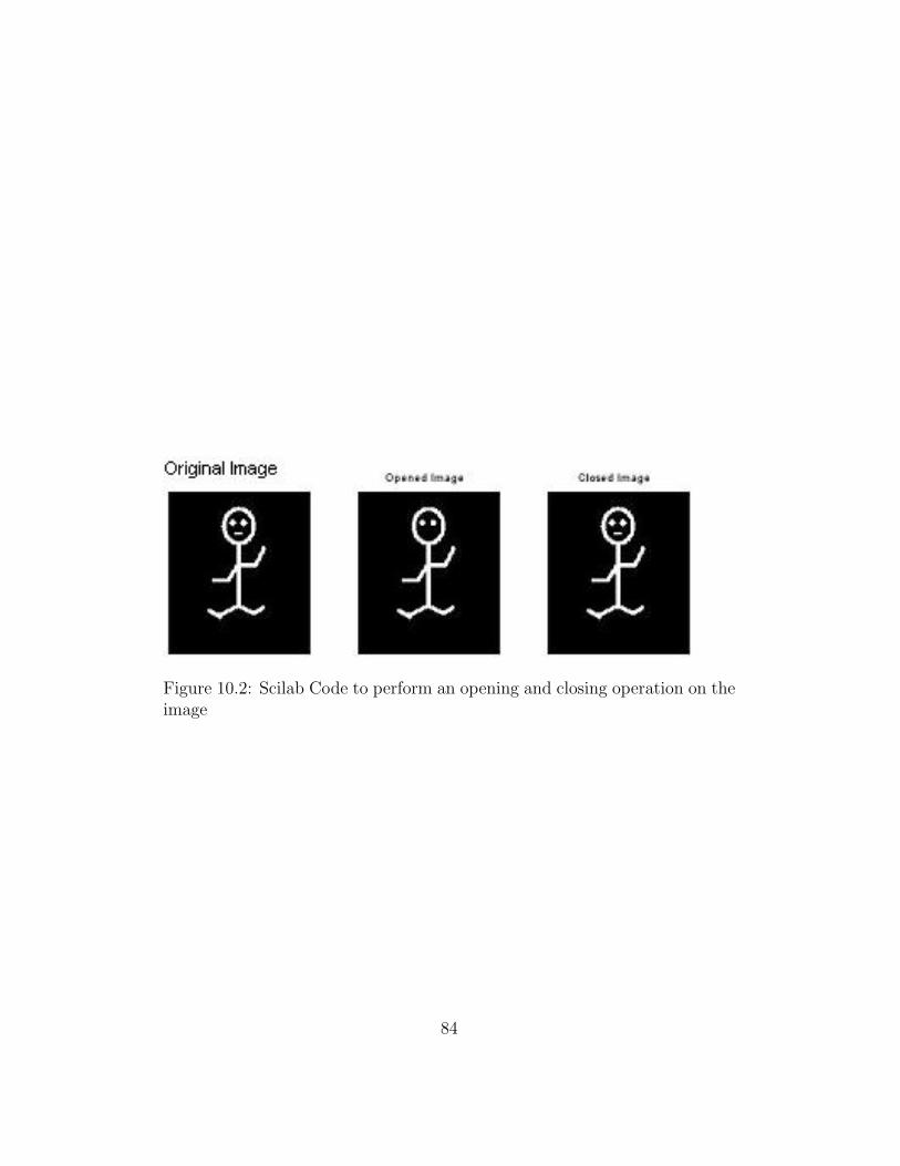
Figure 10.2: Scilab Code to perform an opening and closing operation on theimage
84

Chapter 11
Colur Image Processing
Scilab code Exa 11.4 Read an RGB image and extract the three colourcomponents red green blue
1 // Capt ion : Read an RGB image and e x t r a c t the t h r e ec o l o u r components : red , g r e en
2 // and b lue3 // Fig . 1 1 . 4 : MATLAB Example14 // page5885 clc;
6 close;
7 RGB = imread( ’E : \DIP JAYARAMAN\Chapter11 \ peppe r s . png’ ); //SIVP t o o l b o x
8 R = RGB;
9 G = RGB;
10 B = RGB;
11 R(:,:,2)=0;
12 R(:,:,3)=0;
13 G(:,:,1)=0;
14 G(:,:,3)=0;
15 B(:,:,1)=0;
16 B(:,:,2)=0;
17 figure (1)
18 ShowColorImage(RGB , ’ O r i g i n a l Co lo r Image ’ ); //IPD
85
t o o l b o x19 title( ’ O r i g i n a l Co lo r Image ’ );20 figure (2)
21 ShowColorImage(R, ’ Red Component ’ );22 figure (3)
23 ShowColorImage(G, ’ Green Component ’ );24 figure (4)
25 ShowColorImage(B, ’ Blue Component ’ );
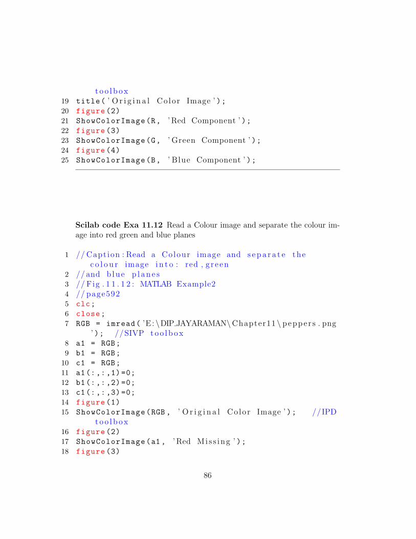
Scilab code Exa 11.12 Read a Colour image and separate the colour im-age into red green and blue planes
1 // Capt ion : Read a Colour image and s e p a r a t e thec o l o u r image i n t o : red , g r e en
2 // and b lue p l a n e s3 // Fig . 1 1 . 1 2 : MATLAB Example24 // page5925 clc;
6 close;
7 RGB = imread( ’E : \DIP JAYARAMAN\Chapter11 \ peppe r s . png’ ); //SIVP t o o l b o x
8 a1 = RGB;
9 b1 = RGB;
10 c1 = RGB;
11 a1(:,:,1)=0;
12 b1(:,:,2)=0;
13 c1(:,:,3)=0;
14 figure (1)
15 ShowColorImage(RGB , ’ O r i g i n a l Co lo r Image ’ ); //IPDt o o l b o x
16 figure (2)
17 ShowColorImage(a1 , ’ Red Mi s s i ng ’ );18 figure (3)
86

Figure 11.1: Read an RGB image and extract the three colour componentsred green blue
87

19 ShowColorImage(b1 , ’ Green Mi s s i ng ’ );20 figure (4)
21 ShowColorImage(c1 , ’ Blue Mi s s i ng ’ );
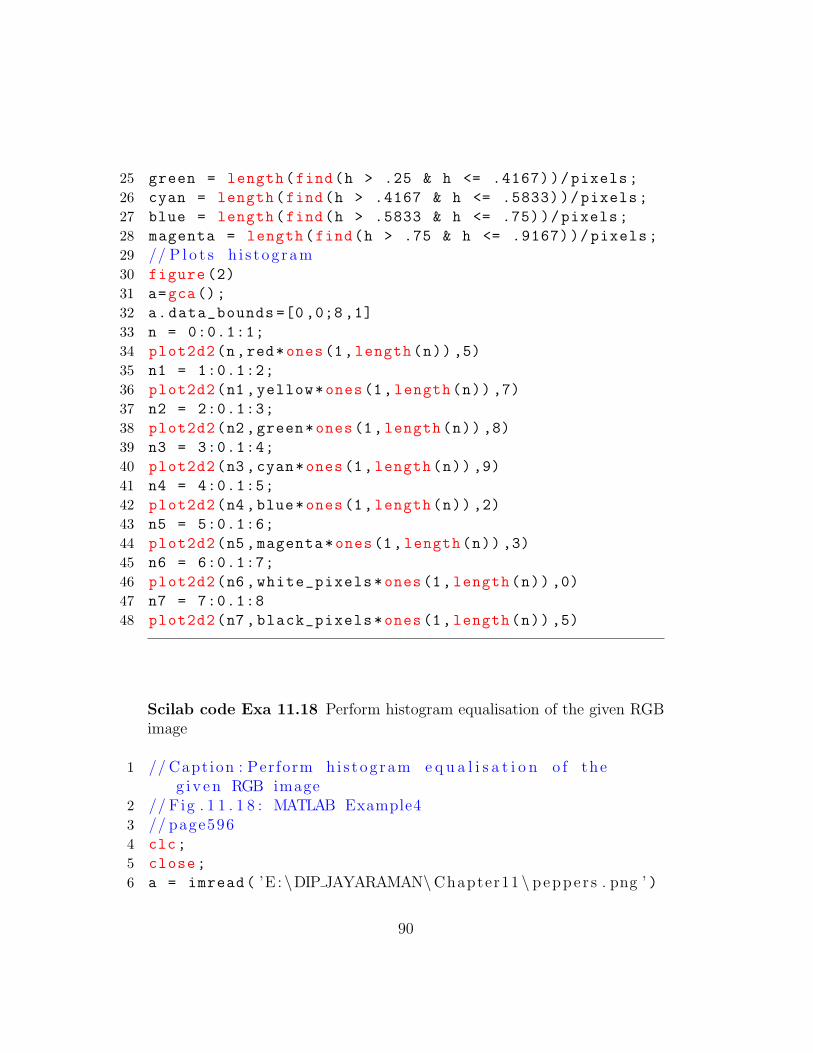
Scilab code Exa 11.16 Compute the histogram of the colour image
1 // Capt ion : Compute the h i s t og ram o f the c o l o u r image2 // Fig . 1 1 . 1 6 : MATLAB Example33 // page5954 clc;
5 close;
6 I = imread( ’E : \DIP JAYARAMAN\Chapter11 \ l a v e n d e r . jpg ’); //SIVP t o o l b o x
7 figure (1)
8 ShowColorImage(I, ’ O r i g i n a l Co lo r Image ’ ); //IPDt o o l b o x
9 J = im2double(I);
10 [index ,map] = RGB2Ind(I); //IPD t o o l b o x11 pixels = prod(size(index));
12 hsv = rgb2hsv(J);
13 h = hsv(:,1);
14 s = hsv(:,2);
15 v = hsv(:,3);
16 // Finds l o c a t i o n o f b l a c k and whi te p i x e l s17 darks = find(v <0.2);
18 lights = find(s<0.05 & v >0.85);
19 h([darks lights ])=-1;
20 // Gets the number o f a l l p i x e l s f o r each c o l o u r b in21 black_pixels = length(darks)/pixels;
22 white_pixels = length(lights)/pixels;
23 red = length(find((h > .9167 | h <= .083) & h ~= -1)
)/pixels;
24 yellow = length(find(h > .083 & h <= .25))/pixels;
88

Figure 11.2: Read a Colour image and separate the colour image into redgreen and blue planes
89
25 green = length(find(h > .25 & h <= .4167))/pixels;
26 cyan = length(find(h > .4167 & h <= .5833))/pixels;
27 blue = length(find(h > .5833 & h <= .75))/pixels;
28 magenta = length(find(h > .75 & h <= .9167))/pixels;
29 // P l o t s h i s t og ram30 figure (2)
31 a=gca();
32 a.data_bounds =[0 ,0;8 ,1]
33 n = 0:0.1:1;
34 plot2d2(n,red*ones(1,length(n)) ,5)
35 n1 = 1:0.1:2;
36 plot2d2(n1,yellow*ones(1,length(n)) ,7)
37 n2 = 2:0.1:3;
38 plot2d2(n2,green*ones(1,length(n)) ,8)
39 n3 = 3:0.1:4;
40 plot2d2(n3,cyan*ones(1,length(n)) ,9)
41 n4 = 4:0.1:5;
42 plot2d2(n4,blue*ones(1,length(n)) ,2)
43 n5 = 5:0.1:6;
44 plot2d2(n5,magenta*ones(1,length(n)) ,3)
45 n6 = 6:0.1:7;
46 plot2d2(n6,white_pixels*ones(1,length(n)) ,0)
47 n7 = 7:0.1:8
48 plot2d2(n7,black_pixels*ones(1,length(n)) ,5)
Scilab code Exa 11.18 Perform histogram equalisation of the given RGBimage
1 // Capt ion : Perform h i s tog ram e q u a l i s a t i o n o f theg i v e n RGB image
2 // Fig . 1 1 . 1 8 : MATLAB Example43 // page5964 clc;
5 close;
6 a = imread( ’E : \DIP JAYARAMAN\Chapter11 \ peppe r s . png ’ )
90

; //SIVP t o o l b o x7 // c o n v e r s i o n o f RGB to YIQ format8 b = rgb2ntsc(a);
9 // Histogram e q u a l i s a t i o n o f Y component a l o n e10 b(:,:,1) =
11 // c o n v e r s i o n o f YIQ to RGB format12 c = ntsc2rgb(b);
13 figure (1)
14 ShowColorImage(a, ’ O r i g i n a l Image ’ ); //IPD t o o l b o x15 figure (2)
16 ShowColorImage(c, ’ H i s togt ram e q u a l i z e d Image ’ );//IPD t o o l b o x
Scilab code Exa 11.21 This program performs median filtering of the colourimage
1 // Capt ion : This program per f o rms median f i l t e r i n g o fthe c o l o u r image
2 // Fig . 1 1 . 2 1 : MATLAB Example53 // page5984 clc;
5 close;
6 a = imread( ’E : \DIP JAYARAMAN\Chapter11 \ peppe r s . png ’ ); //SIVP t o o l b o x
7 b = imnoise(a, ’ s a l t & pepper ’ , 0.2);
8 c(:,:,1)= MedianFilter(b(:,:,1), [3 3]);
9 c(:,:,2)= MedianFilter(b(:,:,2), [3 3]);
10 c(:,:,3)= MedianFilter(b(:,:,3), [3 3]);
11 figure (1)
12 ShowColorImage(a, ’ O r i g i n a l Image ’ ); //IPD t o o l b o x13 figure (2)
14 ShowColorImage(b, ’ c o r r u p t e d Image ’ ); //IPDt o o l b o x
15 figure (3)
16 ShowColorImage(c, ’ Median F i l t e r e d Image ’ ); //IPD
91
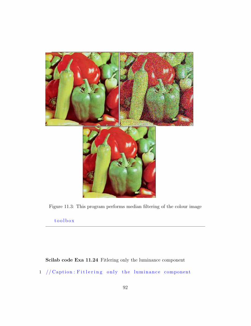
Figure 11.3: This program performs median filtering of the colour image
t o o l b o x
Scilab code Exa 11.24 Fitlering only the luminance component
1 // Capt ion : F i t l e r i n g on ly the luminance component
92
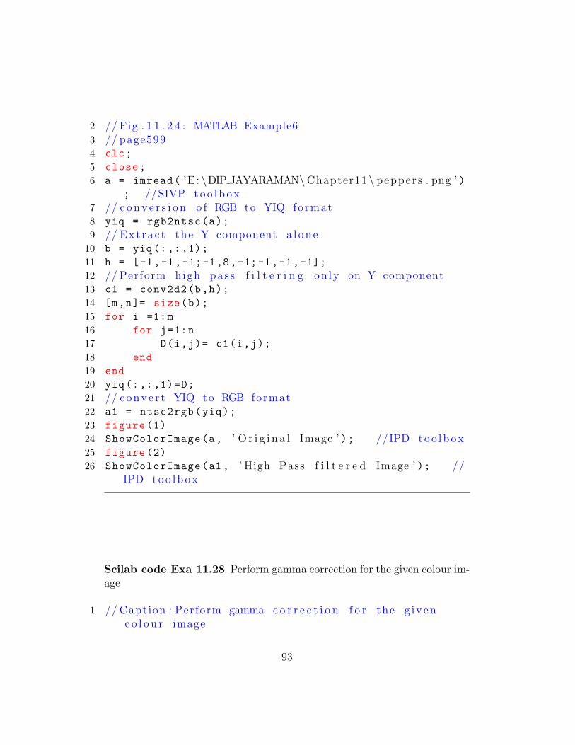
2 // Fig . 1 1 . 2 4 : MATLAB Example63 // page5994 clc;
5 close;
6 a = imread( ’E : \DIP JAYARAMAN\Chapter11 \ peppe r s . png ’ ); //SIVP t o o l b o x
7 // c o n v e r s i o n o f RGB to YIQ format8 yiq = rgb2ntsc(a);
9 // Ext ra c t the Y component a l o n e10 b = yiq(:,:,1);
11 h = [-1,-1,-1;-1,8,-1;-1,-1,-1];
12 // Perform high pas s f i l t e r i n g on ly on Y component13 c1 = conv2d2(b,h);
14 [m,n]= size(b);
15 for i =1:m
16 for j=1:n
17 D(i,j)= c1(i,j);
18 end
19 end
20 yiq(:,:,1)=D;
21 // c o n v e r t YIQ to RGB format22 a1 = ntsc2rgb(yiq);
23 figure (1)
24 ShowColorImage(a, ’ O r i g i n a l Image ’ ); //IPD t o o l b o x25 figure (2)
26 ShowColorImage(a1 , ’ High Pass f i l t e r e d Image ’ ); //IPD t o o l b o x
Scilab code Exa 11.28 Perform gamma correction for the given colour im-age
1 // Capt ion : Perform gamma c o r r e c t i o n f o r the g i v e nc o l o u r image
93
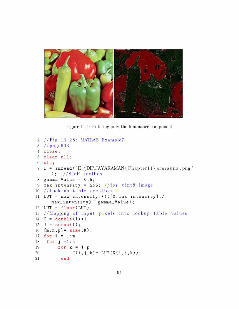
Figure 11.4: Fitlering only the luminance component
2 // Fig . 1 1 . 2 8 : MATLAB Example73 // page6034 close;
5 clear all;
6 clc;
7 I = imread( ’E : \DIP JAYARAMAN\Chapter11 \ ararauna . png ’); //SIVP t o o l b o x
8 gamma_Value = 0.5;
9 max_intensity = 255; // f o r u i n t 8 image10 // Look up t a b l e c r e a t i o n11 LUT = max_intensity .*(([0: max_intensity ]./
max_intensity).^ gamma_Value);
12 LUT = floor(LUT);
13 // Mapping o f i nput p i x e l s i n t o lookup t a b l e v a l u e s14 K = double(I)+1;
15 J = zeros(I);
16 [m,n,p]= size(K);
17 for i = 1:m
18 for j =1:n
19 for k = 1:p
20 J(i,j,k)= LUT(K(i,j,k));
21 end
94
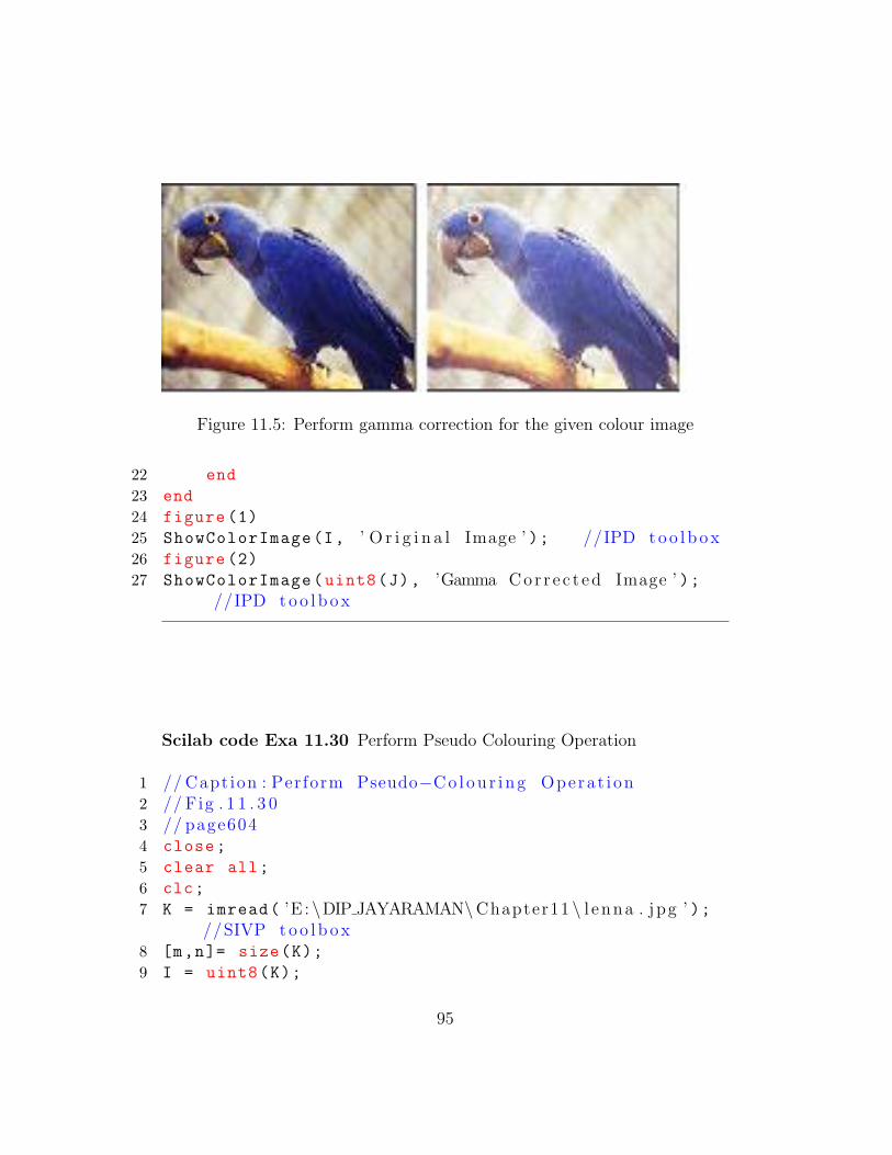
Figure 11.5: Perform gamma correction for the given colour image
22 end
23 end
24 figure (1)
25 ShowColorImage(I, ’ O r i g i n a l Image ’ ); //IPD t o o l b o x26 figure (2)
27 ShowColorImage(uint8(J), ’Gamma Co r r e c t e d Image ’ );//IPD t o o l b o x
Scilab code Exa 11.30 Perform Pseudo Colouring Operation
1 // Capt ion : Perform Pseudo−C o l o u r i n g Operat i on2 // Fig . 1 1 . 3 03 // page6044 close;
5 clear all;
6 clc;
7 K = imread( ’E : \DIP JAYARAMAN\Chapter11 \ l enna . jpg ’ );//SIVP t o o l b o x
8 [m,n]= size(K);
9 I = uint8(K);
95
10 for i = 1:m
11 for j =1:n
12 if (I(i,j) >=0 & I(i,j) <50)
13 J(i,j,1)=I(i,j)+50;
14 J(i,j,2)=I(i,j)+100;
15 J(i,j,3)=I(i,j)+10;
16 elseif (I(i,j) >=50 & I(i,j) <100)
17 J(i,j,1)=I(i,j)+35;
18 J(i,j,2)=I(i,j)+128;
19 J(i,j,3)=I(i,j)+10;
20 elseif(I(i,j) >=100 & I(i,j) <150)
21 J(i,j,1)=I(i,j)+152;
22 J(i,j,2)=I(i,j)+130;
23 J(i,j,3)=I(i,j)+15;
24 elseif(I(i,j) >=150 & I(i,j) <200)
25 J(i,j,1)=I(i,j)+50;
26 J(i,j,2)=I(i,j)+140;
27 J(i,j,3)=I(i,j)+25;
28 elseif(I(i,j) >=200 & I(i,j) <=256)
29 J(i,j,1)=I(i,j)+120;
30 J(i,j,2)=I(i,j)+160;
31 J(i,j,3)=I(i,j)+45;
32 end
33 end
34 end
35 figure (1)
36 ShowImage(K, ’ O r i g i n a l Image ’ ); //IPD t o o l b o x37 figure (2)
38 ShowColorImage(J, ’ Pseudo Coloured Image ’ ); //IPDt o o l b o x
Scilab code Exa 11.32 Read an RGB image and segment it using thethreshold method
96
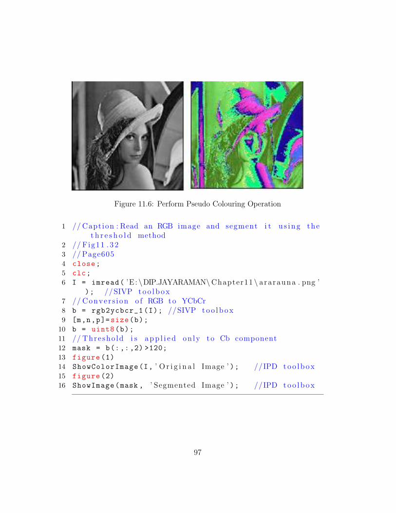
Figure 11.6: Perform Pseudo Colouring Operation
1 // Capt ion : Read an RGB image and segment i t u s i n g thet h r e s h o l d method
2 // Fig11 . 3 23 // Page6054 close;
5 clc;
6 I = imread( ’E : \DIP JAYARAMAN\Chapter11 \ ararauna . png ’); //SIVP t o o l b o x
7 // Conver s i on o f RGB to YCbCr8 b = rgb2ycbcr_1(I); //SIVP t o o l b o x9 [m,n,p]=size(b);
10 b = uint8(b);
11 // Thresho ld i s a p p l i e d on ly to Cb component12 mask = b(:,:,2) >120;
13 figure (1)
14 ShowColorImage(I, ’ O r i g i n a l Image ’ ); //IPD t o o l b o x15 figure (2)
16 ShowImage(mask , ’ Segmented Image ’ ); //IPD t o o l b o x
97
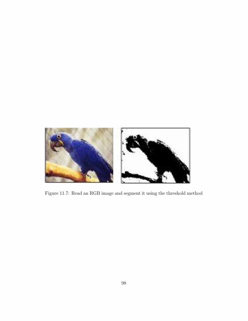
Figure 11.7: Read an RGB image and segment it using the threshold method
98
Chapter 12
Wavelet based ImageProcessing
Scilab code Exa 12.9 Scilab code to perform wavelet decomposition
1 // Capt ion : S c i l a b code to per fo rm wave l e td e c o m p o s i t i o n
2 // Fig12 . 1 03 // Page6244 clc;
5 close;
6 x = ReadImage( ’E : \DIP JAYARAMAN\Chapter12 \ l enna . jpg ’);
7 //The image i n uns i gned i n t e g e r or doub le has to bec o n v e r t e d i n t o no rma l i z e d
8 // doub l e fo rmat9 x = im2double(x);
10 // F i r s t Leve l d e c o m p o s i t i o n11 [CA ,CH,CV,CD]=dwt2(x, ’ db1 ’ );12 // Second l e v e l d e c o m p o s i t i o n13 [CA1 ,CH1 ,CV1 ,CD1]=dwt2(CA , ’ db1 ’ );14 CA = im2int8(CA);
15 CH = im2int8(CH);
16 CV = im2int8(CV);
99
17 CD = im2int8(CD);
18 CA1 = im2int8(CA1);
19 CH1 = im2int8(CH1);
20 CV1 = im2int8(CV1);
21 CD1 = im2int8(CD1);
22 A = [CA,CH;CV,CD];
23 B = [CA1 ,CH1;CV1 ,CD1];
24 imshow(B)
25 title( ’ R e s u l t o f Second Lev e l Decompos i t i on ’ )
Scilab code Exa 12.42 Scilab code to generate different levels of a Gaus-sian pyramid
1 // Capt ion : S c i l a b code to g e n e r a t e d i f f e r e n t l e v e l so f a Gauss ian pyramid
2 // Fig12 . 4 23 // Page6514 clc;
5 close;
6 a = imread( ’E : \DIP JAYARAMAN\Chapter12 \ app l e3 . bmp ’ );7 a = rgb2gray(a);
8 b = a;
9 kernelsize = input( ’ Enter the s i z e o f the k e r n e l : ’ );10 sd = input( ’ Enter the s tandard d e v i a t i o n o f hte
Gauss ian window : ’ );11 rf = input( ’ Enter the Reduct ion Facto r : ’ );12 // Rout ine to g e n e r a t e Gauss ian k e r n e l13 k = zeros(kernelsize , kernelsize);
14 [m n] = size(b);
15 t = 0;
16 for i = 1: kernelsize
17 for j=1: kernelsize
18 k(i,j) = exp(-((i-kernelsize /2) .^2+(j-
kernelsize /2) .^2) /(2*sd.^2))/(2* %pi*sd
.^2);
100

19 t = t+k(i,j);
20 end
21 end
22 for i = 1: kernelsize
23 for j = 1: kernelsize
24 k(i,j) = k(i,j)/t;
25 end
26 end
27 for t = 1:1:rf
28 // c o n v o l v e i t with the p i c t u r e29 FilteredImg = b;
30 if t==1
31 FilteredImg = filter2(k,b)/255;
32 else
33 FilteredImg = filter2(k,b);
34 end;
35 // compute the s i z e o f the reduced image36 m = m/2;
37 n = n/2;
38 // c r e a t e the reduced image through sampl ing39 b = zeros(m,n);
40 for i = 1:m
41 for j = 1:n
42 b(i,j) = FilteredImg(i*2,j*2);
43 end;
44 end;
45 end;
46 figure
47 ShowImage(a, ’ O r i g i n a l Image ’ )48 figure
49 ShowImage(b, ’ D i f f e r e n t L e v e l s o f Gausain Pyramid ’ )50 title( ’ D i f f e r e n t L e v e l s o f Gausain Pyramid Leve l 2 ’ )
101

Figure 12.1: Scilab code to generate different levels of a Gaussian pyramid
102
Scilab code Exa 12.57 Scilab code to implement watermarking in spatialdomain
1 // Capt ion : S c i l a b code to implement watermark ing i ns p a t i a l domain
2 // Fig12 . 5 73 // Page6624 clc
5 close
6 a = imread( ’E : \DIP JAYARAMAN\Chapter12 \cameraman . jpg’ );
7 figure
8 imshow(a)
9 title( ’ Base Image ’ );10 b = imread( ’E : \DIP JAYARAMAN\Chapter12 \ keyimage . jpg ’
);
11 b = rgb2gray(b);
12 b = imresize(b,[32 32], ’ b i c u b i c ’ );13 [m1 n1]=size(b);
14 figure
15 imshow(b)
16 title( ’ Mark Image ’ );17 [m n]=size(a);
18 i1 = 1;
19 j1 = 1;
20 p = 1;
21 c = a;
22 iii = 1;
23 jjj = 1;
24 a = uint8(a);
25 b = uint8(b);
26 for ff = 1:8
27 for i = 1:32
28 jjj = 1;
29 for j = j1:j1+n1 -1
30 a(i,j) = bitand(a(i,j),uint8 (254)); //LSB o f base image i s s e t to z e r o .
31 temp = bitand(b(i,jjj),uint8 ((2^ff) -1));
103
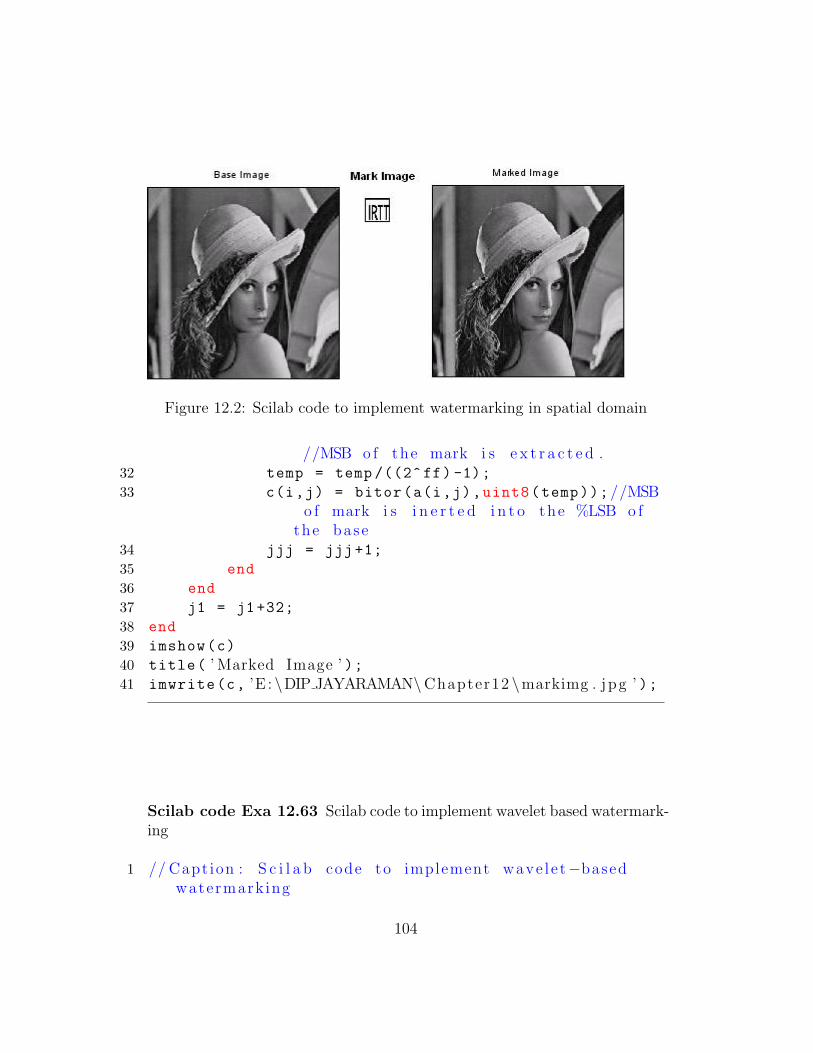
Figure 12.2: Scilab code to implement watermarking in spatial domain
//MSB o f the mark i s e x t r a c t e d .32 temp = temp /((2^ff) -1);
33 c(i,j) = bitor(a(i,j),uint8(temp));//MSBo f mark i s i n e r t e d i n t o the %LSB o f
the base34 jjj = jjj+1;
35 end
36 end
37 j1 = j1+32;
38 end
39 imshow(c)
40 title( ’ Marked Image ’ );41 imwrite(c, ’E : \DIP JAYARAMAN\Chapter12 \markimg . jpg ’ );
Scilab code Exa 12.63 Scilab code to implement wavelet based watermark-ing
1 // Capt ion : S c i l a b code to implement wave le t−basedwatermark ing
104
2 // Fig12 . 6 33 // Page6664 clc;
5 close;
6 // O r i g i n a l Image7 img = imread( ’E : \DIP JAYARAMAN\Chapter12 \cameraman .
jpg ’ );8 figure
9 imshow(img)
10 title( ’ O r i g i n a l Image ’ );11 [p q] = size(img);
12 // Generate the key13 // key = imread ( ’E : \DIP JAYARAMAN\Chapter12 \ keyimg1 .
png ’ ) ;14 // key = i m r e s i z e ( key , [ p q ] ) ;15 key = imread( ’E : \DIP JAYARAMAN\Chapter12 \ keyimage .
jpg ’ );16 key = rgb2gray(key);
17 c = 0.001; // I n i t i a l i s e the we ight o f Watermarking18 figure
19 imshow(key)
20 title( ’ Key ’ );21 // Wavelet t r a n s f o r m o f o r i g i n a l image ( base image )22 img = double(img);
23 key = double(key);
24 [ca ,ch,cv,cd] = dwt2(img , ’ db1 ’ );//Compute 2D wave l e tt r a n s f o r m
25 // Perform the watermark ing26 y = [ca ch;cv cd];
27 Y = y + c*key;
28 p=p/2;
29 q=q/2;
30 for i=1:p
31 for j=1:q
32 nca(i,j) = Y(i,j);
33 ncv(i,j) = Y(i+p,j);
34 nch(i,j) = Y(i,j+q);
35 ncd(i,j) = Y (i+p,j+q);
105
36 end
37 end
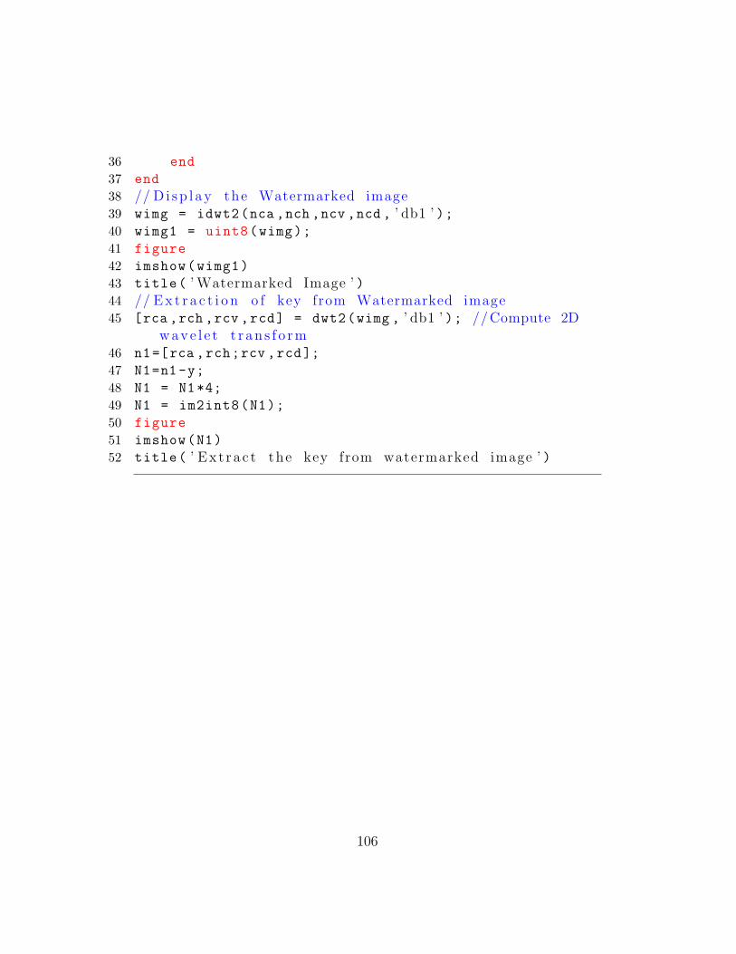
38 // D i s p l a y the Watermarked image39 wimg = idwt2(nca ,nch ,ncv ,ncd , ’ db1 ’ );40 wimg1 = uint8(wimg);
41 figure
42 imshow(wimg1)
43 title( ’ Watermarked Image ’ )44 // E x t r a c t i o n o f key from Watermarked image45 [rca ,rch ,rcv ,rcd] = dwt2(wimg , ’ db1 ’ ); //Compute 2D
wave l e t t r a n s f o r m46 n1=[rca ,rch;rcv ,rcd];
47 N1=n1-y;
48 N1 = N1*4;
49 N1 = im2int8(N1);
50 figure
51 imshow(N1)
52 title( ’ Ex t ra c t the key from watermarked image ’ )
106

Appendix
Scilab code AP 1 2D Fast Fourier Transform
1 function [a2] = fft2d(a)
2 // a = any r e a l o r complex 2D matr ix3 // a2 = 2D−DFT o f 2D matr ix ’ a ’4 m=size(a,1)
5 n=size(a,2)
6 // f o u r i e r t r a n s f o r m a long the rows7 for i=1:n
8 a1(:,i)=exp(-2*%i*%pi *(0:m-1) ’.*.(0:m-1)/m)*a(:,i)
9 end
10 // f o u r i e r t r a n s f o r m a long the columns11 for j=1:m
12 a2temp=exp(-2*%i*%pi *(0:n-1) ’.*.(0:n-1)/n)*(a1(j,:))
.’
13 a2(j,:)=a2temp.’
14 end
15 for i = 1:m
16 for j = 1:n
17 if((abs(real(a2(i,j))) <0.0001)&(abs(imag(a2(
i,j))) <0.0001))
18 a2(i,j)=0;
19 elseif(abs(real(a2(i,j))) <0.0001)
20 a2(i,j)= 0+%i*imag(a2(i,j));
21 elseif(abs(imag(a2(i,j))) <0.0001)
22 a2(i,j)= real(a2(i,j))+0;
23 end
24 end
107

25 end
Scilab code AP 2 2D Inverse FFT
1 function [a] =ifft2d(a2)
2 // a2 = 2D−DFT o f any r e a l o r complex 2D matr ix3 // a = 2D−IDFT o f a24 m=size(a2 ,1)
5 n=size(a2 ,2)
6 // I n v e r s e F o u r i e r t r a n s f o r m a long the rows7 for i=1:n
8 a1(:,i)=exp(2*%i*%pi *(0:m-1) ’.*.(0:m-1)/m)*a2(:,i)
9 end
10 // I n v e r s e f o u r i e r t r a n s f o r m a long the columns11 for j=1:m
12 atemp=exp (2*%i*%pi *(0:n-1) ’.*.(0:n-1)/n)*(a1(j,:)).’
13 a(j,:)=atemp.’
14 end
15 a = a/(m*n)
16 a = real(a)
17 endfunction
Scilab code AP 3 Median Filtering function
1 //The input to the f u n c t i o n a r e the c o r r u p t e d imagea and the d imens ion
2 function [Out_Imag] = Func_medianall(a,N)
3 a=double(a);
4 [m n]=size(a);
5 Out_Imag=a;
6 if(modulo(N,2) ==1)
7 Start=(N+1)/2;
8 End=Start;
9 else
10 Start=N/2;
11 End=Start +1;
12 end
13 if(modulo(N,2) ==1)
108

14 limit1 =(N-1)/2;
15 limit2=limit1;
16 else
17 limit1 =(N/2) -1;
18 limit2=limit1 +1;
19 end
20 for i=Start:(m-End+1),
21 for j=Start:(n-End +1),
22 I=1;
23 for k=-limit1:limit2 ,
24 for l=-limit1:limit2 ,
25 mat(I)=a(i+k,j+l);
26 I=I+1;
27 end
28 end
29 mat=gsort(mat); // So r t the e l e m e n t s tof i n d the median
30 if(modulo(N,2) ==1)
31 Out_Imag(i,j)=(mat(((N^2)+1)/2));
32 else
33 Out_Imag(i,j)=(mat((N^2)/2)+mat (((N^2)/2)
+1))/2;
34 end
35 end
36 end
Scilab code AP 4 To caculate gray level
1 function [g] = gray(m)
2 g = (0:m-1) ’/max(m-1,1)
3 g = [g g g]
4 endfunction
Scilab code AP 5 To change the gray level of gray image
1 function [bout] = grayslice(I,z)
2
109
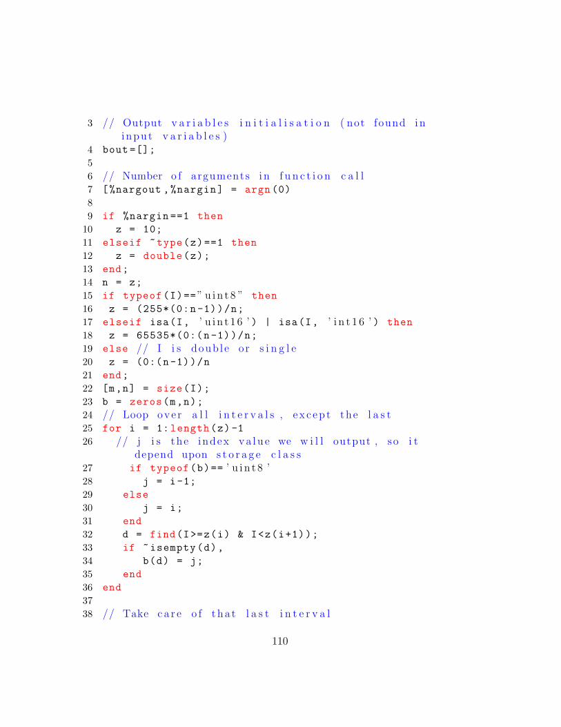
3 // Output v a r i a b l e s i n i t i a l i s a t i o n ( not found i ninput v a r i a b l e s )
4 bout =[];
56 // Number o f arguments i n f u n c t i o n c a l l7 [%nargout ,%nargin] = argn (0)
89 if %nargin ==1 then
10 z = 10;
11 elseif ~type(z)==1 then
12 z = double(z);
13 end;
14 n = z;
15 if typeof(I)==” u i n t 8 ” then
16 z = (255*(0:n-1))/n;
17 elseif isa(I, ’ u i n t 1 6 ’ ) | isa(I, ’ i n t 1 6 ’ ) then
18 z = 65535*(0:(n-1))/n;
19 else // I i s doub le or s i n g l e20 z = (0:(n-1))/n
21 end;
22 [m,n] = size(I);
23 b = zeros(m,n);
24 // Loop ove r a l l i n t e r v a l s , e x c ep t the l a s t25 for i = 1: length(z) -1
26 // j i s the index v a l u e we w i l l output , so i tdepend upon s t o r a g e c l a s s
27 if typeof(b)== ’ u i n t 8 ’28 j = i-1;
29 else
30 j = i;
31 end
32 d = find(I>=z(i) & I<z(i+1));
33 if ~isempty(d),
34 b(d) = j;
35 end
36 end
3738 // Take c a r e o f tha t l a s t i n t e r v a l
110

39 d = find(I >= z($));
40 if ~isempty(d) then
41 // j i s the index v a l u e we w i l l output , so i tdepend upon s t o r a g e c l a s s
42 if typeof(b)==” u i n t 8 ” then
43 j = length(z) -1;
44 else
45 j = length(z);
46 end;
47 b(d) = j;
48 end;
49 bout = b;
50 bout = double(bout);
51 endfunction
111
Related Documents


![[IJET V2I4P9] Authors: Praveen Jayasankar , Prashanth Jayaraman ,Rachel Hannah](https://static.cupdf.com/doc/110x72/588035591a28ab9f0f8b72c5/ijet-v2i4p9-authors-praveen-jayasankar-prashanth-jayaraman-rachel-hannah.jpg)