Digital Image Processing - commsp.ee.ic.ac.uktania/teaching/DIP 2014/DIP HE 2018.pdf · Digital Image Processing Image Enhancement Histogram Equalization DR TANIA STATHAKI READER

Digital Image Processing

Image EnhancementHistogram Equalization

DR TANIA STATHAKIREADER (ASSOCIATE PROFFESOR) IN SIGNAL PROCESSINGIMPERIAL COLLEGE LONDON

• Consider an image with intensity 𝑟𝑘, 𝑘 ∈ [0, 𝐿 − 1] and size 𝑀 ×𝑁.

• The number of pixels with intensity 𝑟𝑘 is 𝑛𝑘.

• The histogram of the image is the function ℎ 𝑟𝑘 = 𝑛𝑘.

• The normalized histogram is the function

𝑝 𝑟𝑘 =𝑛𝑘

𝑀𝑁for 𝑘 = 0,… , 𝐿 − 1

Histogram Processing: definition of image histogram

dark

image

bright

image

low

contrast

image

high

contrast

image

Generic figures of histograms

• The appearance of

histogram reveals a lot of

information about

the contrast of the image and

the mean gray level.

• An image of low contrast has

a histogram that is concentrated

around a small range of

intensities.

• Images of high contrast are

more interesting and pleasant

for the human eye.

Two different images with the same histogram

• The appearance of

histogram reveals a lot of

information about

the contrast of the image and

the mean gray level BUT :

• It doesn’t give any information

regarding the location or the

type of objects present

in the image. This information

is important because it is related

to the image content.

• Two images can have identical

histograms and still be

completely different in terms of

content.

• Consider for the moment continuous intensity values 𝑟 ∈ [0, 𝐿 − 1].

• The value 𝑟 = 0 represents black and the value 𝑟 = 𝐿 − 1 represents white.

• We are looking for intensity transformations of the form:𝑠 = 𝑇 𝑟 , 0 ≤ 𝑟 ≤ 𝐿 − 1.

• The following conditions are imposed on 𝑇 𝑟 :

o 𝑇(𝑟) is monotonically increasing in 0 ≤ 𝑟 ≤ 𝐿 − 1 or strictly monotonically increasing in 0 ≤ 𝑟 ≤ 𝐿 − 1.➢ The above condition guarantees that ordering of the output intensity

values will follow the ordering of the input intensity values (avoids reversal of intensities).

➢ If 𝑇(𝑟) is strictly monotonically increasing then the mapping from 𝑠back to 𝑟 will be 1-1.

o 0 ≤ 𝑇(𝑟) ≤ 𝐿 − 1 for 0 ≤ 𝑟 ≤ 𝐿 − 1.This condition guarantees that the range of intensities of the output will be the same as the range of inthe input.

Histogram Processing: definition of intensity transformation

• In the above Figure on the left we cannot perform inverse mapping (from 𝑠 to 𝑟).

• In the above Figure on the right inverse mapping is possible.

Monotonicity versus strict monotonicity

Modelling intensities as continuous variables

• Assume that an original intensity 𝑟 is mapped to an intensity 𝑠 through the transformation 𝑠 = 𝑇(𝑟).

• We can view intensities 𝑟 and 𝑠 as random variables.

• Instead of histograms we use probability density functions (pdf) 𝑝𝑟(𝑟) and 𝑝𝑠(𝑠).

• Consider a minimal increment of the original intensity 𝑟 to the intensity 𝑟 +𝑑𝑟.

• The intensity 𝑟 + 𝑑𝑟 is mapped to an intensity 𝑠 + 𝑑𝑠 through the transformation 𝑇(𝑟).

• Since 𝑇(𝑟) is (monotonically) increasing we can easily say that 𝑠 + 𝑑𝑠 ≥ 𝑠.

• All values of the original intensity which are within the interval [𝑟, 𝑟 + 𝑑𝑟]will be mapped to new values within the interval [𝑠, 𝑠 + 𝑑𝑠].

• We can say that:

Probability(𝑟 ≤ original intensity ≤ 𝑟 + 𝑑𝑟)=Probability(𝑠 ≤ new intensity ≤𝑠 + 𝑑𝑠) or in mathematical terms:

𝑟𝑟+𝑑𝑟

𝑝𝑟 𝑤 𝑑𝑤 = 𝑠𝑠+𝑑𝑠

𝑝𝑠 𝑤 𝑑𝑤

Modelling intensities as continuous variables cont.

• Probability(𝑟 ≤ original intensity ≤ 𝑟 + 𝑑𝑟)=Probability(𝑠 ≤ new intensity ≤𝑠 + 𝑑𝑠) or in mathematical terms:

𝑟𝑟+𝑑𝑟


𝑝𝑠 𝑤 𝑑𝑤

• If 𝑑𝑟 is small enough we can assume that 𝑝𝑟 𝑟 remains almost constant within the interval [𝑟, 𝑟 + 𝑑𝑟] and equal to 𝑝𝑟 𝑟 .

• We can choose 𝑑𝑟 to be as small as to be able to assume that 𝑑𝑠 is small enough and that 𝑝𝑠 𝑠 remains almost constant within the interval [𝑠, 𝑠 +𝑑𝑠] and equal to 𝑝𝑠 𝑠 .

• 𝑟𝑟+𝑑𝑟


𝑝𝑠 𝑤 𝑑𝑤 ⇒ 𝑝𝑟 𝑟 𝑑𝑟 = 𝑝𝑠 𝑠 𝑑𝑠

• The above analysis is depicted in the Figure of the next slide.

Modelling intensities as continuous variables

Histogram Equalization: continuous form

• A transformation of particular importance in Image Processing is the cumulative distribution function (CDF) of a random variable.

𝑠 = 𝑇 𝑟 = (𝐿 − 1)න0

𝑟

𝑝𝑟 𝑤 𝑑𝑤

• It is an increasing function since for 𝑟2 ≥ 𝑟1 we see that:

𝑠2 = 𝑇 𝑟2 = 𝐿 − 1 0𝑟2 𝑝𝑟 𝑤 𝑑𝑤

= 𝐿 − 1 0𝑟1 𝑝𝑟 𝑤 𝑑𝑤 + 𝐿 − 1 𝑟1

𝑟2 𝑝𝑟 𝑤 𝑑𝑤

= 𝑇 𝑟1 + 𝐿 − 1 𝑟1𝑟2 𝑝𝑟 𝑤 𝑑𝑤 ≥ 𝑇 𝑟1

Histogram Equalization: continuous form

• We showed previously that 𝑝𝑟 𝑟 𝑑𝑟 = 𝑝𝑠 𝑠 𝑑𝑠

• Therefore, 𝑝𝑠 𝑠 =𝑝𝑟 𝑟𝑑𝑠

𝑑𝑟

.

• From the definition

𝑠 = 𝑇 𝑟 = (𝐿 − 1)න0

𝑟


we have that:𝑑𝑠

𝑑𝑟=

𝑑𝑇(𝑟)

𝑑𝑟= (𝐿 − 1)

𝑑

𝑑𝑟0𝑟𝑝𝑟 𝑤 𝑑𝑤 = 𝐿 − 1 𝑝𝑟 𝑟

Hence, 𝑝𝑠 𝑠 =𝑝𝑟 𝑟𝑑𝑠

𝑑𝑟

=𝑝𝑟 𝑟

𝐿−1 𝑝𝑟 𝑟=

1

(𝐿−1), 𝑠 = 1,… , 𝐿 − 1.

Therefore, the new variable 𝑠 is uniformly distributed.

Histogram Equalization: discrete case

• The formula for histogram equalisation in the discrete case is given by a straightforward modification of the formula that corresponds to the continuous-time case.

• Instead of probability density functions (pdf) 𝑝𝑟(𝑟) and 𝑝𝑠(𝑠) we now use histograms.

• The discrete input intensity 𝑟𝑘 is mapped onto a new discrete intensity 𝑠𝑘through the following transformation:

𝑠𝑘 = 𝑇 𝑟𝑘 = (𝐿 − 1)σ𝑗=0𝑘 𝑝𝑟 𝑟𝑗 =

(𝐿−1)

𝑀𝑁σ𝑗=0𝑘 𝑛𝑗.

𝑟𝑘: input intensity

𝑠𝑘: new intensity

𝑛𝑗: frequency of intensity 𝑗

𝑀𝑁: total number of image pixels

Histogram Equalization: discrete case cont.

• In the ideal continuous case histogram equalization produces a new variable 𝑠 which is uniformly distributed.

• In the discrete case the histogram of the new discrete variable 𝑠𝑘 is far from flat but:

o The new histogram is still much more stretched (extended) than the original histogram.

o The new intensity variable always reaches white since

𝑠𝐿−1 = 𝑇 𝑟𝐿−1 = (𝐿 − 1)

𝑗=0

𝐿−1

𝑝𝑟 𝑟𝑗 = 𝐿 − 1

o In other words, this process usually results in an enhanced image, with an increase in the dynamic range of pixel values.

0 50 100 150 200 250 3000

500

1000

1500

2000

2500

3000

0 50 100 150 2000

500

1000

1500

2000

2500

3000

• In the Figures below you can see how histogram could look like after equalizing a digital image.

• It is more “extended” and slightly “flatter” compared to the original histogram

Before equalization After equalization

Histogram Equalization: discrete case cont.

Histogram Equalization: Examples






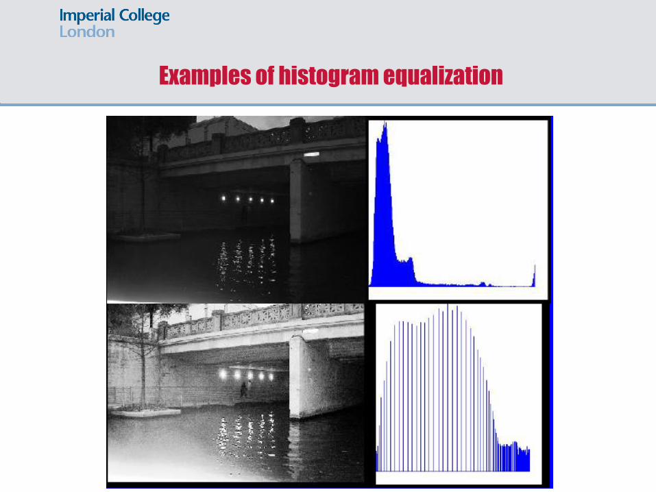
Examples of histogram equalization

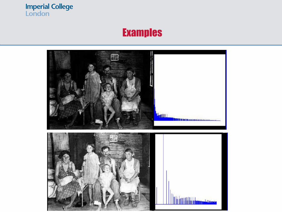
Examples

Histogram equalization may not always produce desirable results, particularly

if the given histogram is very narrow. It can produce false edges and false

regions. It can also increase image “graininess” and “patchiness.”

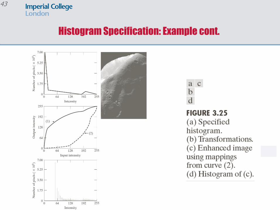
Histogram Equalization is not always desirable

• Example of image of Phobos (Mars moon) and its histogram.

• Histogram equalization (bottom of right image) does not always provide the

desirable results.

Another example of an unfortunate histogram equalization

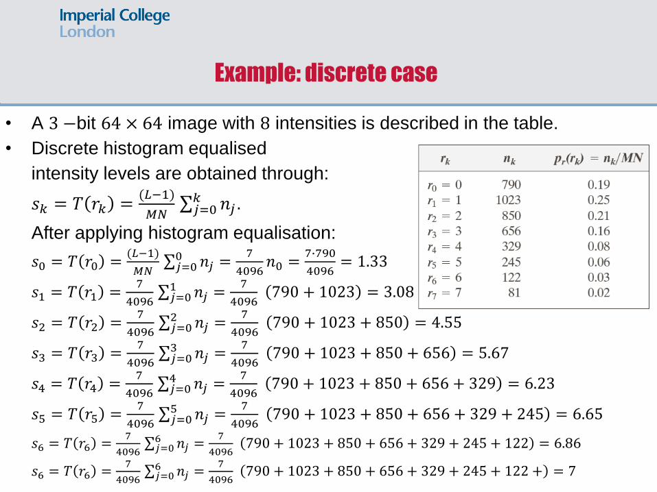
Example: discrete case

• A 3 −bit 64 × 64 image with 8 intensities is described in the table.

• Discrete histogram equalised

intensity levels are obtained through:

𝑠𝑘 = 𝑇 𝑟𝑘 =(𝐿−1)


After applying histogram equalisation:

𝑠0 = 𝑇 𝑟0 =(𝐿−1)

𝑀𝑁σ𝑗=00 𝑛𝑗 =

7

4096𝑛0 =

7∙790

4096= 1.33

𝑠1 = 𝑇 𝑟1 =7

4096σ𝑗=01 𝑛𝑗 =

7

4096790 + 1023 = 3.08

𝑠2 = 𝑇 𝑟2 =7

4096σ𝑗=02 𝑛𝑗 =

7

4096790 + 1023 + 850 = 4.55

𝑠3 = 𝑇 𝑟3 =7

4096σ𝑗=03 𝑛𝑗 =

7

4096790 + 1023 + 850 + 656 = 5.67

𝑠4 = 𝑇 𝑟4 =7

4096σ𝑗=04 𝑛𝑗 =

7

4096790 + 1023 + 850 + 656 + 329 = 6.23

𝑠5 = 𝑇 𝑟5 =7

4096σ𝑗=05 𝑛𝑗 =

7

4096790 + 1023 + 850 + 656 + 329 + 245 = 6.65

𝑠6 = 𝑇 𝑟6 =7

4096σ𝑗=06 𝑛𝑗 =

7

4096790 + 1023 + 850 + 656 + 329 + 245 + 122 = 6.86

𝑠6 = 𝑇 𝑟6 =7

4096σ𝑗=06 𝑛𝑗 =

7

4096790 + 1023 + 850 + 656 + 329 + 245 + 122 + = 7

By rounding to the nearest integer we get:

𝑠0 = 1.33 → 1, 𝑠1 = 3.08 → 3, 𝑠2 = 4.55 → 5, 𝑠3 = 5.67 → 6

𝑠4 = 6.23 → 6, 𝑠5 = 6.65 → 7 𝑠6 = 6.86 → 7, 𝑠7 = 7 → 7

The histogram of the new variable is found

as follows:𝑝 0 = 0𝑝 1 = 𝑝 𝑠0 = 𝑝 𝑟0 = 0.19𝑝 2 = 0𝑝 3 = 𝑝 𝑠1 = 𝑝 𝑟1 = 0.25𝑝 4 = 0𝑝 5 = 𝑝 𝑠2 = 𝑝 𝑟2 = 0.21𝑝 6 = 𝑝 𝑠3 + 𝑝 𝑠4 = 𝑝 𝑟3 + 𝑝 𝑟4 = 0.24𝑝 7 = 𝑝 𝑠5 + 𝑝 𝑠6 + 𝑝 𝑠7 = 𝑝 𝑟5 + 𝑝 𝑟6 + 𝑝 𝑟7 = 0.1

Example: discrete case cont.

Refer to the following figures for original histogram, transformation function and new histogram.


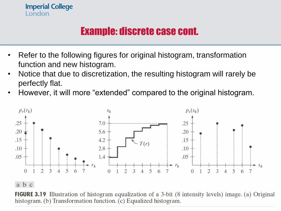
• Refer to the following figures for original histogram, transformation

function and new histogram.

• Notice that due to discretization, the resulting histogram will rarely be

perfectly flat.

• However, it will more “extended” compared to the original histogram.


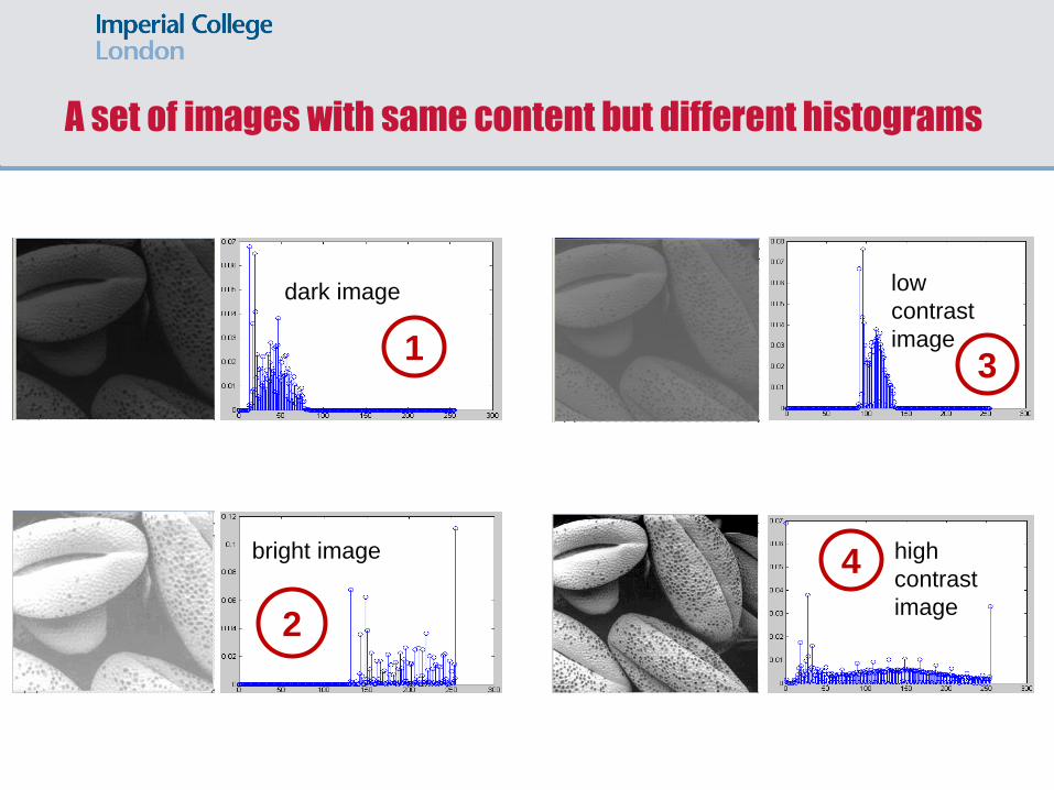
A set of images with same content but different histograms

dark image

bright image

low

contrast

image

high

contrast

image

1

2

3

4

1

Histogram equalization applied to the dark image

2

Histogram equalization applied to the bright image

3

4

Histogram equalization applied

to the low and high contrast images

Transformation functions for histogram equalization

for the previous example

• The function 𝑇(𝑟) used to equalize the four images of the previous example is

shown below.

• Observe that the transformation function in cases 1,2,3 maps a small range of

intensities to the entire range of intensities.

• Observe that for an image which is already bright, the transformation is an almost

diagonal line.

Histogram Specification

• We are looking for a technique which can provide an image with any pre-specified histogram.

• This is called histogram specification.

• We assume that the original image has pdf 𝑝𝑟(𝑟).

• We are looking for a transformation 𝑧 = 𝑇(𝑟) which provides an image with a specific pdf 𝑝𝑧(𝑧) .

• This technique will use histogram equalization as an intermediate step.

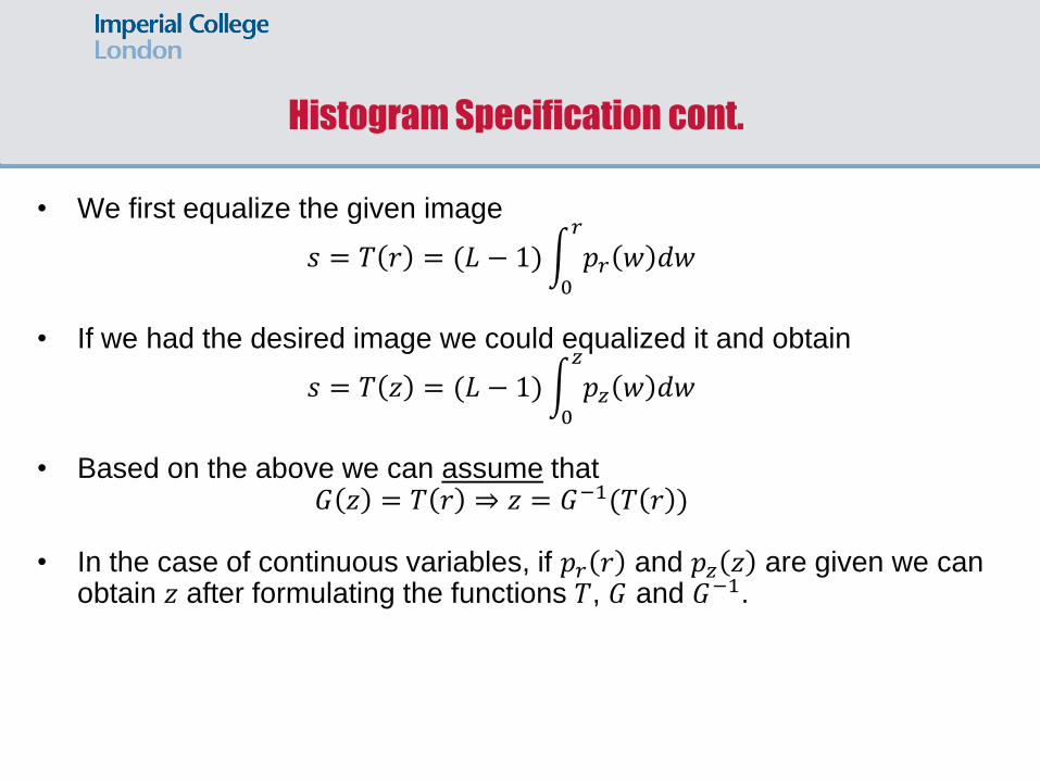
Histogram Specification cont.

• We first equalize the given image

𝑠 = 𝑇 𝑟 = (𝐿 − 1)න0

𝑟


• If we had the desired image we could equalized it and obtain

𝑠 = 𝑇 𝑧 = (𝐿 − 1)න0

𝑧

𝑝𝑧 𝑤 𝑑𝑤

• Based on the above we can assume that𝐺 𝑧 = 𝑇 𝑟 ⇒ 𝑧 = 𝐺−1(𝑇 𝑟 )

• In the case of continuous variables, if 𝑝𝑟 𝑟 and 𝑝𝑧 𝑧 are given we can obtain 𝑧 after formulating the functions 𝑇, 𝐺 and 𝐺−1.

Histogram Specification: continuous form

• In the discrete case we first equalize the initial histogram of the image:

𝑠𝑘 = 𝑇 𝑟𝑘 = (𝐿 − 1)σ𝑗=0𝑘 𝑝𝑟 𝑟𝑗 =

(𝐿−1)


• Then we equalize the target histogram

𝑠𝑘 = 𝐺 𝑧𝑞 = (𝐿 − 1)σ𝑖=0𝑞

𝑝𝑧 𝑟𝑖 =(𝐿−1)


• Finally, we try to obtain some type of inverse transform

𝑧𝑞 = 𝐺−1 𝑠𝑘 = 𝐺−1 𝑇 𝑟𝑘

original

intensities

number of

pixels

probability cumulative

probability

CM

equalised

intensities

CM x 7

normalised

equalised

intensities

0 790 0.19 0.19 1.33 1

1 1023 0.25 0.44 3.08 3

2 850 0.21 0.65 4.55 5

3 656 0.16 0.81 5.67 6

4 329 0.08 0.89 6.23 6

5 245 0.06 0.95 6.65 7

6 122 0.03 0.98 6.86 7

7 81 0.02 1 7 7

Histogram Specification: Example

desired

intensities

probability cumulative

probability

CM

equalised

intensities

CM x 7

normalised

equalised

intensities

0 0 0 0 0

1 0 0 0 0

2 0 0 0 0

3 0.15 0.15 1.05 1

4 0.2 0.35 2.45 2

5 0.3 0.65 4.55 5

6 0.2 0.85 5.95 6

7 0.15 1 7 7

Histogram Specification: Example cont.

desired

intensities

equalised

intensities

(NOT AVAILABLE!!!)

0 0

1 0

2 0

3 1

4 2

5 5

6 6

7 7

original

intensities

equalised

intensities

(AVAILABLE)

0 1

1 3

2 5

3 6

4 6

5 7

6 7

7 7

equalised

intensities

(available)

1

3

5

6

6

7

7

7

NEW

intensities

(available)

3

4

5

6

6

7

7

7


Notice that due to discretization, the resulting histogram will

rarely be exactly the same as the desired histogram.

• Top left: original pdf

• Top right: desired pdf

• Bottom left: desired CDF

• Bottom right: resulting pdf



42


43



• In many cases histograms are needed for local areas of an image.

• Possible applications could be:

o Pattern detection based on histogram.

o Adaptive enhancement.

o Adaptive thresholding.

o Object tracking based on histogram.

Local Histogram Equalization

Local Histogram Equalization for local image enhancement

• The histogram processing methods discussed previously are global

(transformation is based on the intensity distribution of the entire image).

• This global approach is suitable for overall enhancement.

• There are cases in which it is necessary to enhance details over small

areas in an image.

• The number of pixels in these areas may have negligible influence on

the computation of a global transformation.

• The solution is to devise transformation functions based on the intensity

distribution in a neighbourhood around every pixel.

• carry other tasks such as detection, tracking and spatially adaptive

thresholding.

Example: Local Histogram Equalization


• Observe the details revealed with local (spatially adaptive) histogram

equalization.

Top left: A window size of [25 25]. Top right: A window size of [64 64].

Bottom left: A window size of [100 100]. Bottom right: A window size of [200 200].


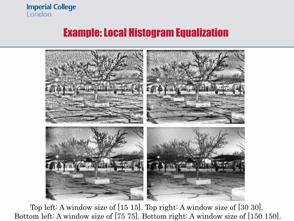
Top left: A window size of [15 15]. Top right: A window size of [30 30].

Bottom left: A window size of [75 75]. Bottom right: A window size of [150 150].



• Image is split into smaller regions and the traditional histogram

equalization is applied to each region.

• The smaller equalized images are combined into one to obtain a final

resultant image.

• The final image appears to be very blocky in nature and has different

contrast levels for each individual region.

• Post-processing is required to remove the blocking artifacts.

Example: Local Histogram Equalization drawbacks

Digital Image Processing - commsp.ee.ic.ac.uktania/teaching/DIP 2014/DIP HE 2018.pdf · Digital Image Processing Image Enhancement Histogram Equalization DR TANIA STATHAKI READER

Documents