Digital Image Processing Vahid Meghdadi Reference: Digital Image processing by Rafael Gonzalz

Welcome message from author
This document is posted to help you gain knowledge. Please leave a comment to let me know what you think about it! Share it to your friends and learn new things together.
Transcript
Digital Image
ProcessingVahid Meghdadi
Reference: Digital Image processing by Rafael
Gonzalz

Course chart
• 4 classes of 1h20 each
• 2 lab on Matlab
• One written examination

Fundamentals
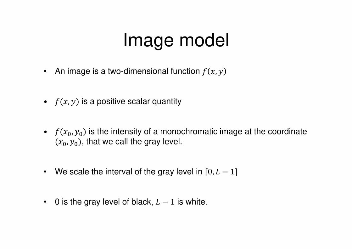
Image model
• An image is a two-dimensional function � �, �• �(�, �) is a positive scalar quantity
• �(��, ��) is the intensity of a monochromatic image at the coordinate (��, ��), that we call the gray level.
• We scale the interval of the gray level in [0, � − 1]• 0 is the gray level of black, � − 1 is white.

Image sampling and
quantification
� �
�
• The result of sampling in the space (� and �) is the pixelation.
• The result of sampling in the gray level is the quantification.

Image representing
• The image is then represented by a two-dimensional matrix
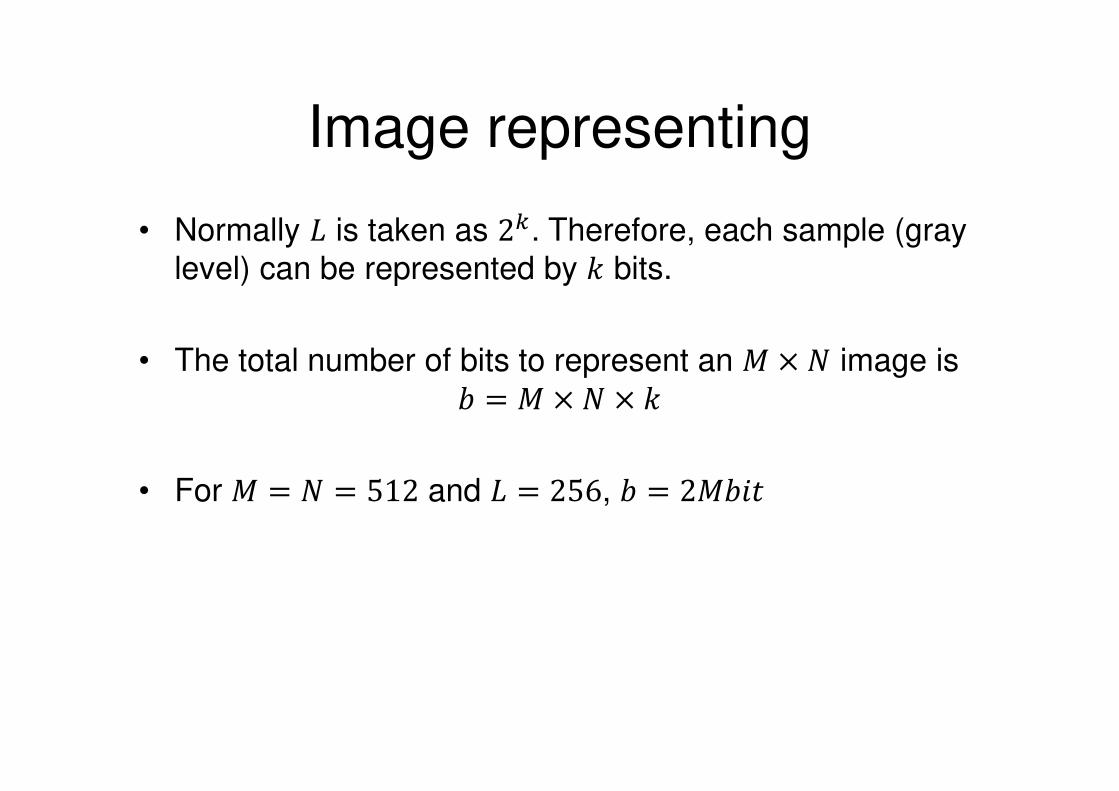
Image representing
• Normally � is taken as 2�. Therefore, each sample (gray
level) can be represented by � bits.
• The total number of bits to represent an � × � image is� = � × � × �• For � = � = 512 and � = 256, � = 2����

100 200 300 400 500
100
200
300
400
100 200 300 400 500
100
200
300
400
100 200 300 400 500
100
200
300
400
100 200 300 400 500
100
200
300
400
Quantification
8 bits
3 bits1 bit
5 bits

50 100 150 200 250 300 350 400 450 500
50
100
150
200
250
300
350
400
450
Quantification error
Quantification error for � = 2 (� = 1 bit)
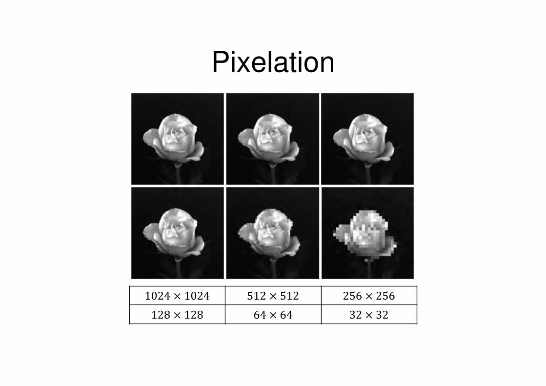
Pixelation
1024 × 1024 512 × 512 256 × 256128 × 128 64 × 64 32 × 32

Matlab commands
• Reading an image fileim = imread(‘c:\image_dir\lenna.jpg’);
• To display an imageimshow(im);
• To change the formatimwrite (im,’c:\image_dir\lenna.bmp’);

Shifting
�� = � + �; �� = � + �#$ ��, �� = #% �, � = #%(�� − �, �� − �)

Example : Shift
1 0 0 2 0 0 3 0 0 4 0 0 5 0 0
5 0
1 0 0
1 5 0
2 0 0
2 5 0
3 0 0
3 5 0
4 0 0
4 5 0
1 0 0 2 0 0 3 0 0 4 0 0 5 0 0
5 0
1 0 0
1 5 0
2 0 0
2 5 0
3 0 0
3 5 0
4 0 0
4 5 0
I2(x,y)=I1((x-240) mod 480 , (y-270) mod 540)

Zooming
• Zooming requires two steps: creation of new pixel
locations, and assigning values to those new locations
• An image of size (10 × 10) becomes an image of size
(20 × 20)
• Results checkerboard effect
Integer factor Non-integer factor

zoming• #%(�, �) is the initial image• #$(�′, �′) is the zoomed image
#$ ��, �� = #% �, ��� = (� − ��)', �� = � − �� (#$ �, � = #% ��' + ��, ��( + ��

Example
(200,230)
x=200+round(x’/alpha); y=230+round(y’/beta);
b(x',y')=a(x,y); % alpha=beta=4
Shrinking
• Shrinking is a reduction in the size
• The process is the column-row deletion of the
image matrix.

Rotation
#$ ��, �� = #% �, � = #%(�� cos , + �� sin , , −�� sin , + �� cos ,)

Example: Rotation
Teta=90° Teta=20°

Exercice :"Shear" suivant x
x=x'-round(cos(teta)*y'); y=y'; %teta = 30°
�� = � + �. tan , ; �� = �

Neighbors of a pixel
• A pixel at (�, �) has for direct neighbors :� + 1, � , � − 1, � , �, � + 1 , �(� − 1)
• We can extend this notion to the neighborhood
Rectangular neighborhood Circular
neighborhood
Intensity
transformation in the
spatial domain
Image enhancement
• The objective is to improve the visual quality of
the image
• The space domain refers to direct manipulation
of the intensity (gray level) of pixels.
• The performance evaluation is “subjective”.

Background
• Spatial domain transformation is denoted by < �, � = =[�(�, �)]where �(�, �) is the input image, <(�, �) is the processed
image, and = is an operator on �, defined over some
neighborhood of (�, �).
�(�, �) < �, � a function of �(�, �) on the
neighborhood

Intensity mapping
• The simplest neighborhood is of size 1 × 1• In this case < �, � = = � �, �> = =(?)• The simplest one is
constant multiplier: > = @. ?• This transformation is to
increase the intensity of the
picture.

Constant multiplication
5 0 1 0 0 1 5 0 2 0 0 2 5 0
5 0
1 0 0
1 5 0
2 0 0
2 5 0
5 0 1 0 0 1 5 0 2 0 0 2 5 0
5 0
1 0 0
1 5 0
2 0 0
2 5 0
Constante = 5
0, 51 → (0, 255) and 52, 255 → 255

Negative image
In general > = = ? = � − 1 − ?For the special case of � = 255,
> = 255 − ?
This transformation gives a negative image.

Négation
1 0 0 2 0 0 3 0 0 4 0 0
5 0
1 0 0
1 5 0
2 0 0
2 5 0
3 0 0
3 5 0
4 0 0
4 5 0
5 0 0
5 5 0
1 0 0 2 0 0 3 0 0 4 0 0
5 0
1 0 0
1 5 0
2 0 0
2 5 0
3 0 0
3 5 0
4 0 0
4 5 0
5 0 0
5 5 0
Matlab code

Binary transformation
Threshold = 70

Seuillage
Seuil = 50
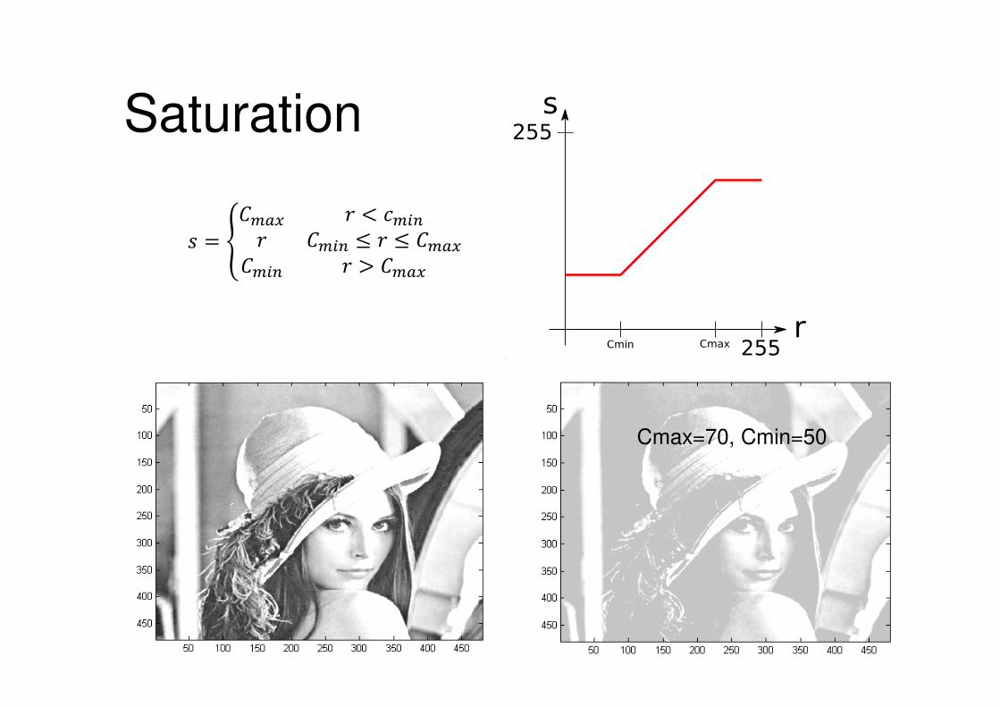
Saturation
Cmax=70, Cmin=50
> = F@GHI ? < KGLM? @GLM ≤ ? ≤ @GHI@GLM ? > @GHI

Adjusting
Re-scale to obtain 8 bits after "saturating".
The preceding picture can
be re-scaled to cover the
range [0 − � − 1]
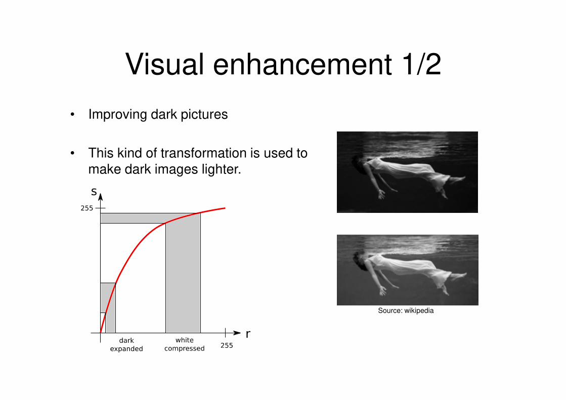
Visual enhancement 1/2
• Improving dark pictures
• This kind of transformation is used to make dark images lighter.
Source: wikipedia
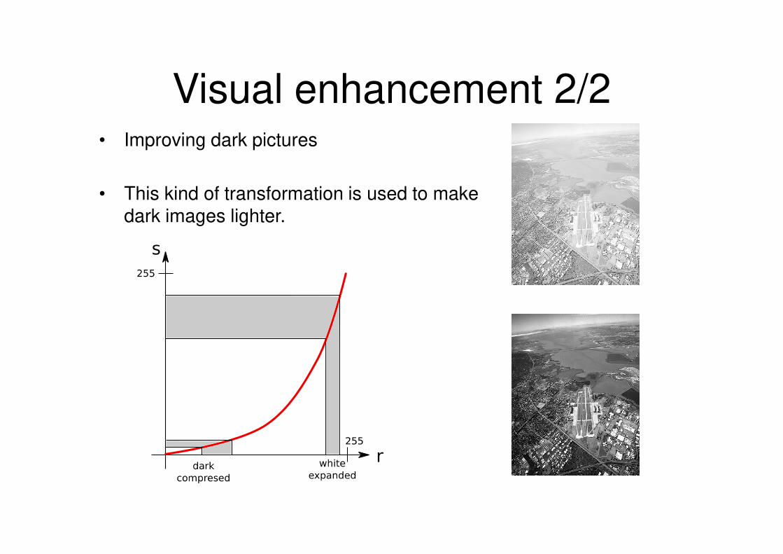
Visual enhancement 2/2• Improving dark pictures
• This kind of transformation is used to make dark images lighter.

Logarithmic Transformation
• The general form of log transformation:> = K log(1 + ?)where K is a constant.
• To transform 0, � − 1 to 0, � − 1 , K = � − 1log �• This transformation enhances the dark zone of the
image but saturates the light zones.

Example
50 100 150 200 250
50
100
150
200
250
50 100 150 200 250
50
100
150
200
250
After a Fourier transform, the dynamic of the picture is too important. The
log transform helps to see the details in the dark zones. The same
process has been seen in the dB representation of the transfer functions.
> = K log(1 + ?)
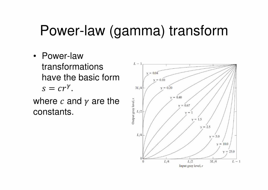
Power-law (gamma) transform
• Power-law
transformations
have the basic form > = K?P .where K and Q are the
constants.

Power-law (gamma)
Original image too dark
Power-law correction with gamma = 0.6
100 200 300
50
100
150
200
250
300
350
400
450
100 200 300
50
100
150
200
250
300
350
400
450
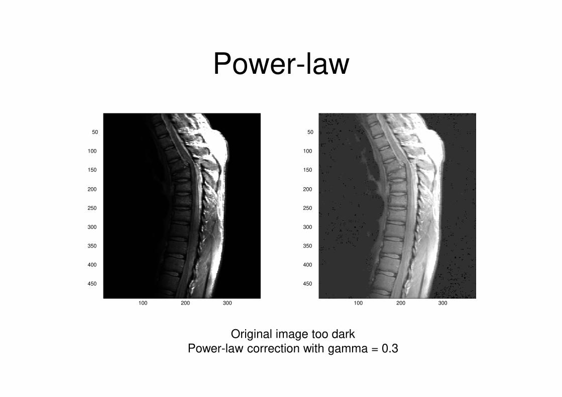
Power-law
Original image too dark
Power-law correction with gamma = 0.3
100 200 300
50
100
150
200
250
300
350
400
450
100 200 300
50
100
150
200
250
300
350
400
450

200 400 600
100
200
300
400
500
600
700
200 400 600
100
200
300
400
500
600
700
Original image too light
Power-law correction with gamma = 2
Power-law

Power-law
200 400 600
100
200
300
400
500
600
700
200 400 600
100
200
300
400
500
600
700
Original image too light
Power-law correction with gamma = 4
Histogram processing
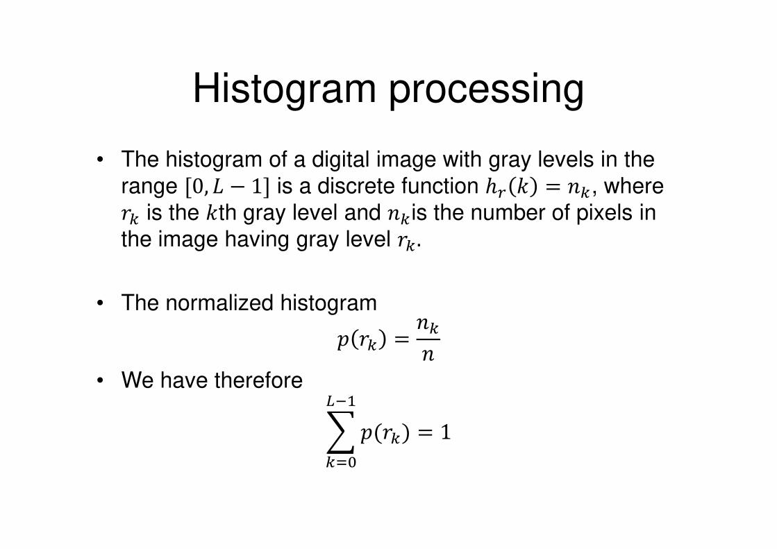
• The histogram of a digital image with gray levels in the
range [0, � − 1] is a discrete function ℎS � = T�, where ?� is the �th gray level and T�is the number of pixels in
the image having gray level ?� .• The normalized histogram U ?� = T�T• We have therefore
V U(?�)WX%�Y� = 1

Histogram example
1 0 0 2 0 0 3 0 0 4 0 0 5 0 0
5 0
1 0 0
1 5 0
2 0 0
2 5 0
3 0 0
3 5 0
4 0 0
4 5 0
5 0 00 5 0 1 0 0 1 5 0 2 0 0 2 5 0
0
0 . 0 1
0 . 0 2
0 . 0 3
0 . 0 4
0 . 0 5
0 . 0 6
0 . 0 7
Dark picture

Histogram
1 0 0 2 0 0 3 0 0 4 0 0 5 0 0
5 0
1 0 0
1 5 0
2 0 0
2 5 0
3 0 0
3 5 0
4 0 0
4 5 0
5 0 00 5 0 1 0 0 1 5 0 2 0 0 2 5 0
0
0 . 0 2
0 . 0 4
0 . 0 6
0 . 0 8
0 . 1
0 . 1 2
Bright picture
Histogram
1 0 0 2 0 0 3 0 0 4 0 0 5 0 0
5 0
1 0 0
1 5 0
2 0 0
2 5 0
3 0 0
3 5 0
4 0 0
4 5 0
5 0 00 5 0 1 0 0 1 5 0 2 0 0 2 5 0
0
0 . 0 1
0 . 0 2
0 . 0 3
0 . 0 4
0 . 0 5
0 . 0 6
0 . 0 7
0 . 0 8
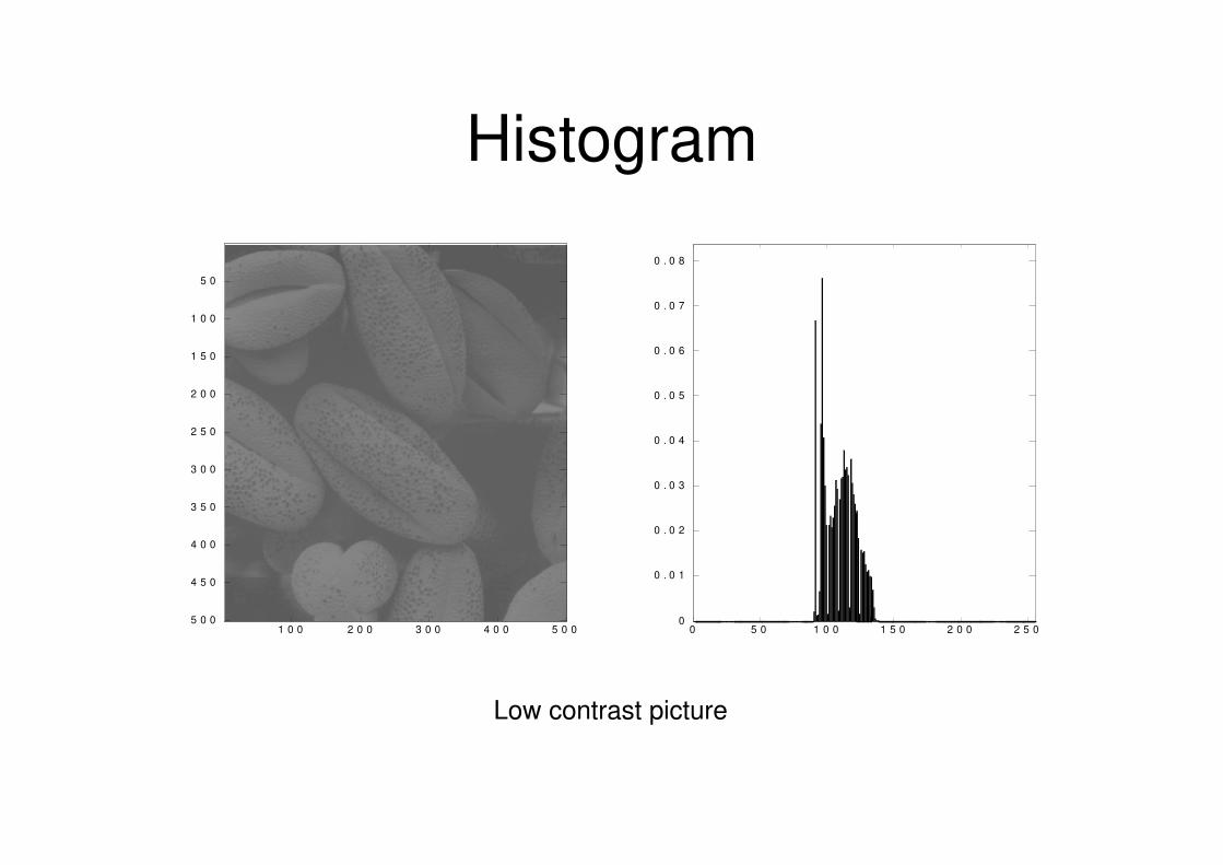
Low contrast picture
Histogram
1 0 0 2 0 0 3 0 0 4 0 0 5 0 0
5 0
1 0 0
1 5 0
2 0 0
2 5 0
3 0 0
3 5 0
4 0 0
4 5 0
5 0 00 5 0 1 0 0 1 5 0 2 0 0 2 5 0
0
0 . 0 1
0 . 0 2
0 . 0 3
0 . 0 4
0 . 0 5
0 . 0 6
0 . 0 7
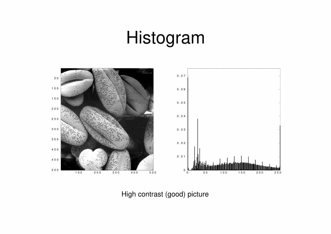
High contrast (good) picture

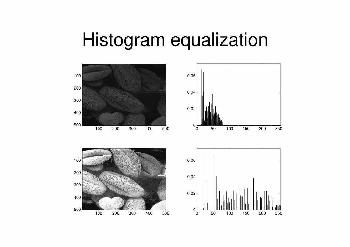
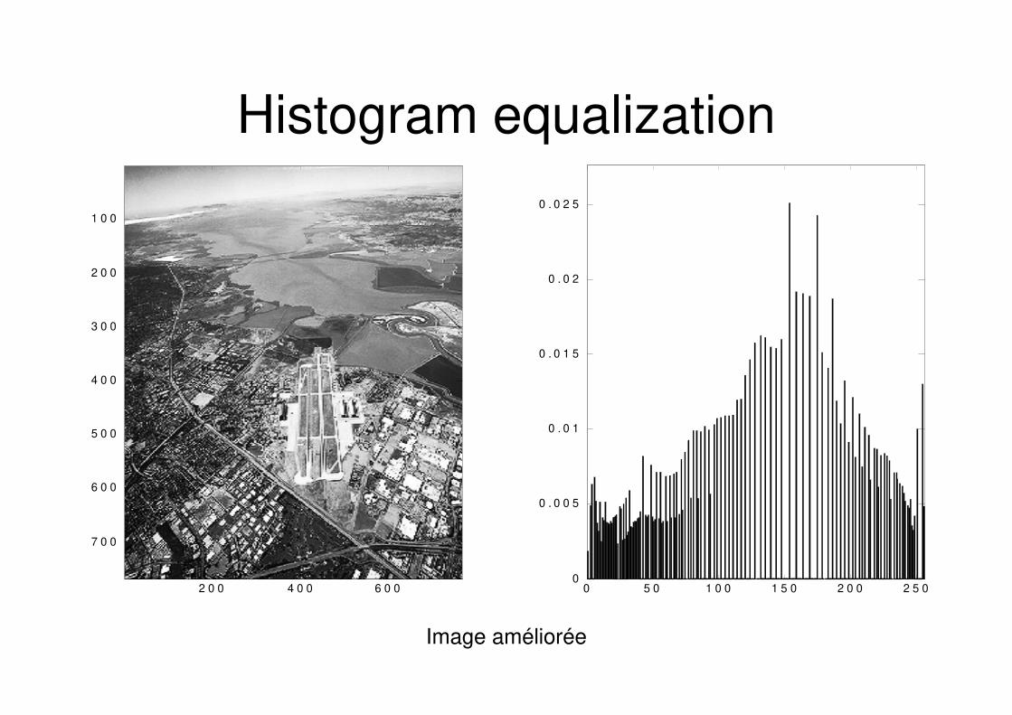
Histogram equalization
• AT first, assume that ? is normalized to be in the interval 0,1 .• We are looking for > = =(?)• The function = ? is obviously monotonically increasing
in 0 ≤ ? ≤ 1, and 0 ≤ = ? ≤ 1.
• The inverse function is: ? = =X% > 0 ≤ > ≤ 1.

Histogram equalization• The ? can be considered as a random variable wityh the pdf as US ? .• The output gray level is also a RV with UZ(>).
• The problem is to find a transformation =(?) such that the UZ > be
uniformly distributed: UZ(>) = 1• With the previous assumptions:
UZ > = US(?) ? >Therefore, if UZ > = 1,
> = = ? = [ US � �S�

Histogram equalization
• In the case of digital images, there is just discrete
values. In this caseUS ?� = M\M for � = 0,1, … , � − 1• The discrete version of the integral will be
>� = = ?� = V US(?̂ )�^Y� = V T̂T
�^Y�
So, for each gray level, on can compute an output gray
level.

Histogram equalization
• This method does not have any parameters.
• Well adapted for automatic processing
• The output histogram is not always uniform but the
output is nearly optimal in terms of contrast.
• The implementation is very easy.
• It is used in digital cameras.
Histogram equalization
100 200 300 400 500
100
200
300
400
5000 50 100 150 200 250
0
0.02
0.04
0.06
100 200 300 400 500
100
200
300
400
5000 50 100 150 200 250
0
0.02
0.04
0.06
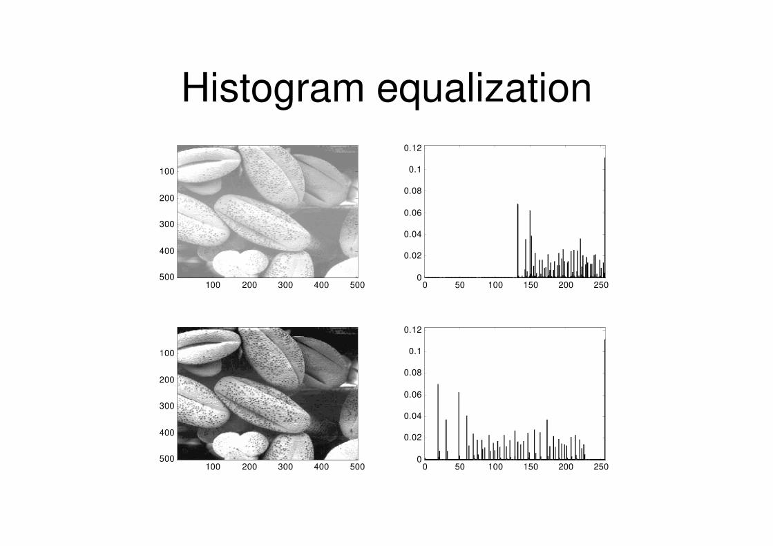
Histogram equalization
100 200 300 400 500
100
200
300
400
5000 50 100 150 200 250
0
0.02
0.04
0.06
0.08
0.1
0.12
100 200 300 400 500
100
200
300
400
5000 50 100 150 200 250
0
0.02
0.04
0.06
0.08
0.1
0.12

Histogram equalization
100 200 300 400 500
100
200
300
400
5000 50 100 150 200 250
0
0.02
0.04
0.06
0.08
100 200 300 400 500
100
200
300
400
5000 50 100 150 200 250
0
0.02
0.04
0.06
0.08

Histogram equalization
100 200 300 400 500
100
200
300
400
5000 50 100 150 200 250
0
0.02
0.04
0.06
100 200 300 400 500
100
200
300
400
5000 50 100 150 200 250
0
0.02
0.04
0.06

Histogram equalization
2 0 0 4 0 0 6 0 0
1 0 0
2 0 0
3 0 0
4 0 0
5 0 0
6 0 0
7 0 0
0 5 0 1 0 0 1 5 0 2 0 0 2 5 00
0 . 0 0 5
0 . 0 1
0 . 0 1 5
0 . 0 2
0 . 0 2 5
Image de départ
2 0 0 4 0 0 6 0 0
1 0 0
2 0 0
3 0 0
4 0 0
5 0 0
6 0 0
7 0 0
0 5 0 1 0 0 1 5 0 2 0 0 2 5 00
0 . 0 0 5
0 . 0 1
0 . 0 1 5
0 . 0 2
0 . 0 2 5
Image améliorée
Histogram equalization

2 0 0 4 0 0 6 0 0
1 0 0
2 0 0
3 0 0
4 0 0
5 0 0
6 0 0
7 0 0
2 0 0 4 0 0 6 0 0
1 0 0
2 0 0
3 0 0
4 0 0
5 0 0
6 0 0
7 0 0
Histogram equalization
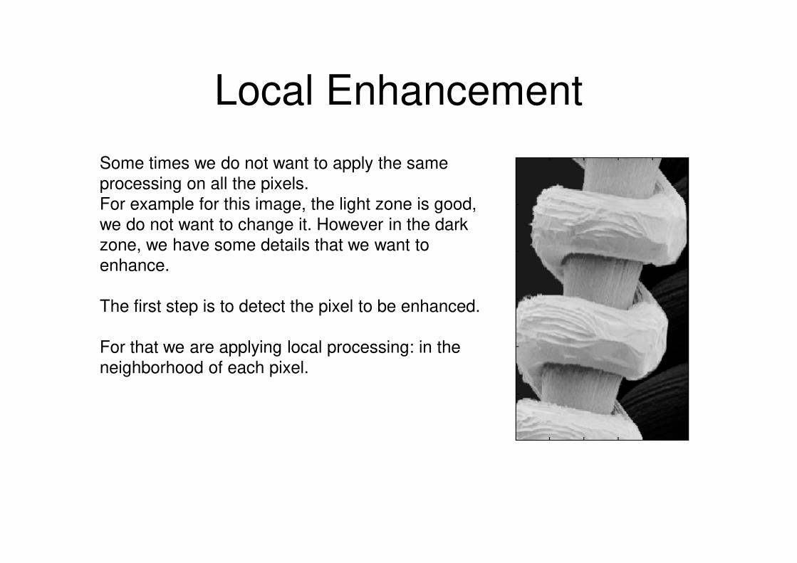
Local Enhancement
Some times we do not want to apply the same
processing on all the pixels.
For example for this image, the light zone is good,
we do not want to change it. However in the dark
zone, we have some details that we want to
enhance.
The first step is to detect the pixel to be enhanced.
For that we are applying local processing: in the
neighborhood of each pixel.
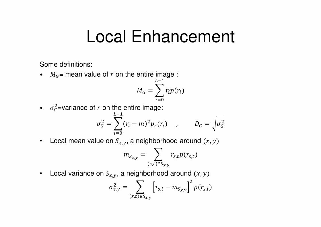
Local Enhancement
Some definitions:• �_= mean value of ? on the entire image :
�_ = V ?LU(?L)WX%LY�• `_$=variance of ? on the entire image:
`_$ = V ?L − a $US(?L)WX%LY� , b_ = `_$c
• Local mean value on dI,e, a neighborhood around (�, �)afg,h = V ?Z,iU(?Z,i)c
Z,i ∈fg,h• Local variance on dI,e, a neighborhood around (�, �)
`I,e$ = V ?Z,i − afg,h$ U(?Z,i)c
Z,i ∈fg,h
Local enhancement
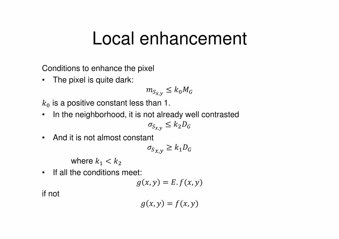
Conditions to enhance the pixel
• The pixel is quite dark: afg,h ≤ ���_�� is a positive constant less than 1.
• In the neighborhood, it is not already well contrasted
f̀g,h ≤ �$b_• And it is not almost constant
f̀I,e ≥ �%b_where �% < �$
• If all the conditions meet:< �, � = l. �(�, �)if not < �, � = �(�, �)

Local enhancement
E=4, K0=0.4, K1=0.02, K2=0.4
Enhanced zonesEnhanced imageOriginal image

moyennage
Image bruitéImage d'origine Image améliorée
4 itérations
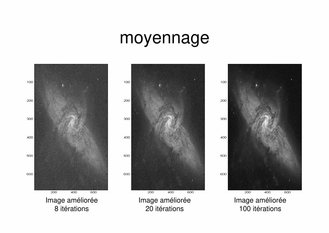
moyennage
Image améliorée
100 itérations
Image améliorée
20 itérations
Image améliorée
8 itérations
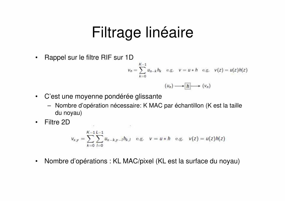
Filtrage linéaire
• Rappel sur le filtre RIF sur 1D
• C’est une moyenne pondérée glissante
– Nombre d’opération nécessaire: K MAC par échantillon (K est la taille
du noyau)
• Filtre 2D
• Nombre d’opérations : KL MAC/pixel (KL est la surface du noyau)

Filtre 2D séparable
• Filtre 2D séparable en deux filtres 1D, un filtre horizontal
et un filtre vertical
• Complexité = K+L MAC par pixel au lieu de KL
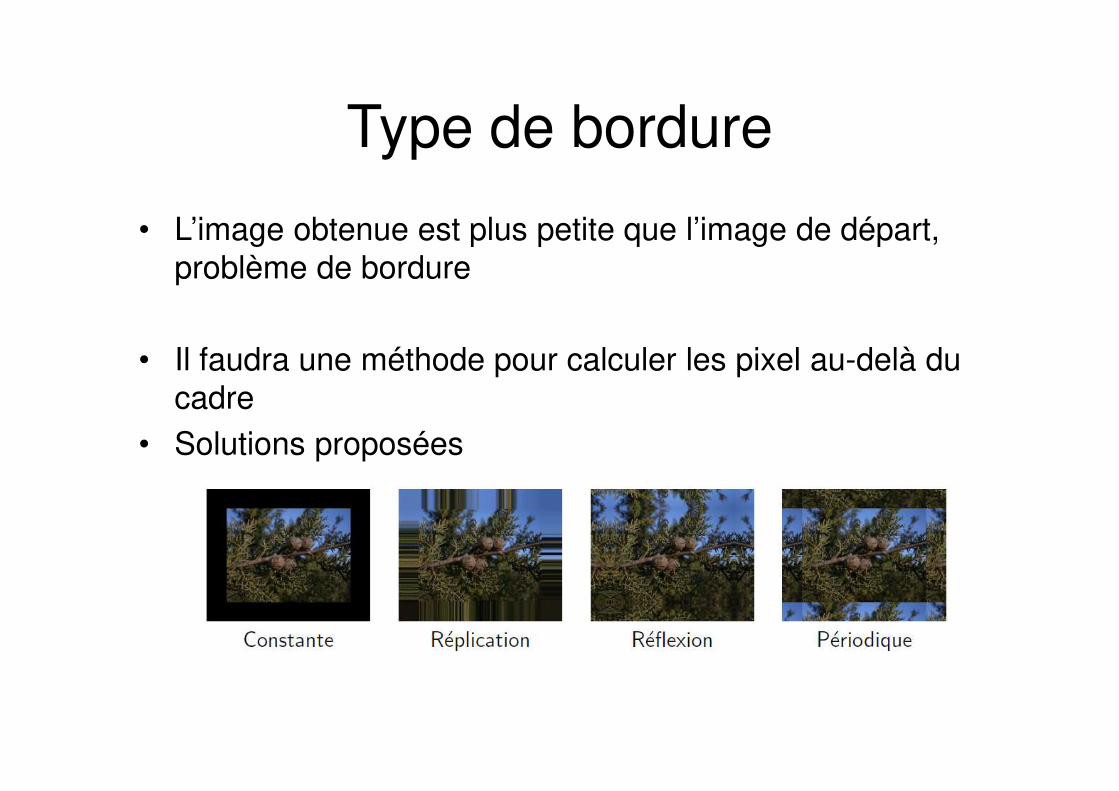
Type de bordure
• L’image obtenue est plus petite que l’image de départ,
problème de bordure
• Il faudra une méthode pour calculer les pixel au-delà du
cadre
• Solutions proposées

Filtre à moyenne mobile
• Filtre rectangulaire avec le noyau constant
• Résultat : image moins bruitée, mais plus floue
• Exemple pour 3x3

Moyenne mobile noyau
constant
Image d'origine Masque 5*5
Masque 5*5 avec pondération Masque 9*9
Filtre à moyenne mobile
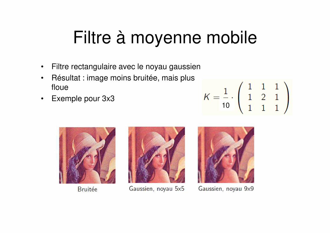
• Filtre rectangulaire avec le noyau gaussien
• Résultat : image moins bruitée, mais plus floue
• Exemple pour 3x310

1 1 2 2 2 1 1
1 2 3 4 3 2 1
2 3 5 5 5 3 21
2 4 5 6 5 4 2132
2 3 5 5 5 3 2
1 2 3 4 3 2 1
1 1 2 2 2 1 1
2 2
22
1( , )
2
x y
h x y e σ
πσ
+−=
Masque gaussien
0 0 1 0 0
0 2 2 2 01
1 2 5 2 125
0 2 2 2 0
0 0 1 0 0
1 2 3 2 1
2 4 6 4 21
3 6 9 6 381
2 4 6 4 2
1 2 3 2 1
Masque triangulaire
Masque circulaire
Masque (filtre)

Filtre médiane
• Si il existe des pixels erronés isolés
• C’est un filtre non linéaire
• Chaque pixel est remplacé par la médiane des valeurs
de son voisinage
50 62 67 56 255 70 60 0 48 52
x 62 62 67 70 70 60 48 48 x
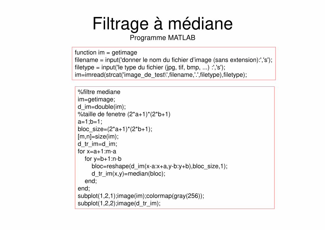
%filtre mediane
im=getimage;
d_im=double(im);
%taille de fenetre (2*a+1)*(2*b+1)
a=1;b=1;
bloc_size=(2*a+1)*(2*b+1);
[m,n]=size(im);
d_tr_im=d_im;
for x=a+1:m-a
for y=b+1:n-b
bloc=reshape(d_im(x-a:x+a,y-b:y+b),bloc_size,1);
d_tr_im(x,y)=median(bloc);
end;
end;
subplot(1,2,1);image(im);colormap(gray(256));
subplot(1,2,2);image(d_tr_im);
function im = getimage
filename = input('donner le nom du fichier d’image (sans extension):','s');
filetype = input('le type du fichier (jpg, tif, bmp, ...) :','s');
im=imread(strcat('image_de_test\',filename,'.',filetype),filetype);
Filtrage à médianeProgramme MATLAB

Filtrage à médiane
Médiane 3*3 Médiane 5*5
Moyennage 3*3Image d'origine
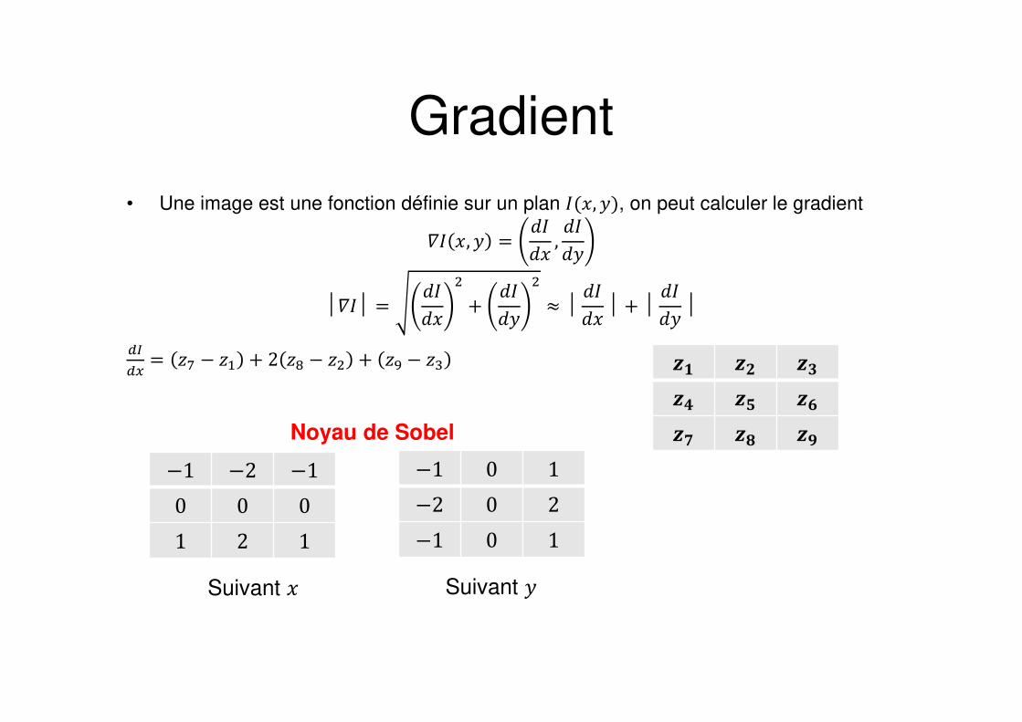
Gradient
• Une image est une fonction définie sur un plan #(�, �), on peut calculer le gradient
m# �, � = # � , # �│m#│ = # �
$ + # �$c ≈ │ # � │ + │ # � │
pqpI = rs − r% + 2 rt − r$ + ru − rv wx wy wzw{ w| w}w~ w� w�−1 −2 −10 0 01 2 1Suivant �
−1 0 1−2 0 2−1 0 1Suivant �
Noyau de Sobel

Opérateur Sobel
−1 −2 −10 0 01 2 1−1 0 1−2 0 2−1 0 1
Application: détection de contours

Méthode gradient (Sobel)
2 0 0 4 0 0 6 0 0 8 0 0
1 0 0
2 0 0
3 0 0
4 0 0
5 0 0
6 0 0
7 0 0
8 0 0
9 0 0
2 0 0 4 0 0 6 0 0 8 0 0
1 0 0
2 0 0
3 0 0
4 0 0
5 0 0
6 0 0
7 0 0
8 0 0
9 0 0
Approximation valeur absolue
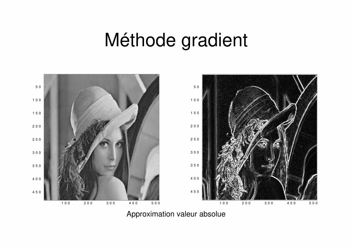
Méthode gradient
1 0 0 2 0 0 3 0 0 4 0 0 5 0 0
5 0
1 0 0
1 5 0
2 0 0
2 5 0
3 0 0
3 5 0
4 0 0
4 5 0
1 0 0 2 0 0 3 0 0 4 0 0 5 0 0
5 0
1 0 0
1 5 0
2 0 0
2 5 0
3 0 0
3 5 0
4 0 0
4 5 0
Approximation valeur absolue
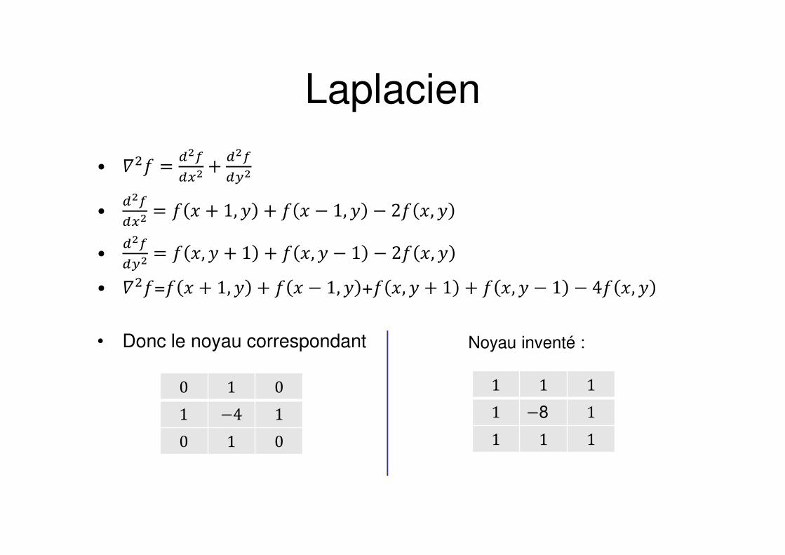
Laplacien
• m$� = p��pI� + p��pe�• p��pI� = � � + 1, � + � � − 1, � − 2� �, �• p��pe� = � �, � + 1 + � �, � − 1 − 2� �, �• m$�=� � + 1, � + � � − 1, � +� �, � + 1 + � �, � − 1 − 4� �, �• Donc le noyau correspondant
0 1 01 −4 10 1 0
Noyau inventé :
1 1 11 −8 11 1 1
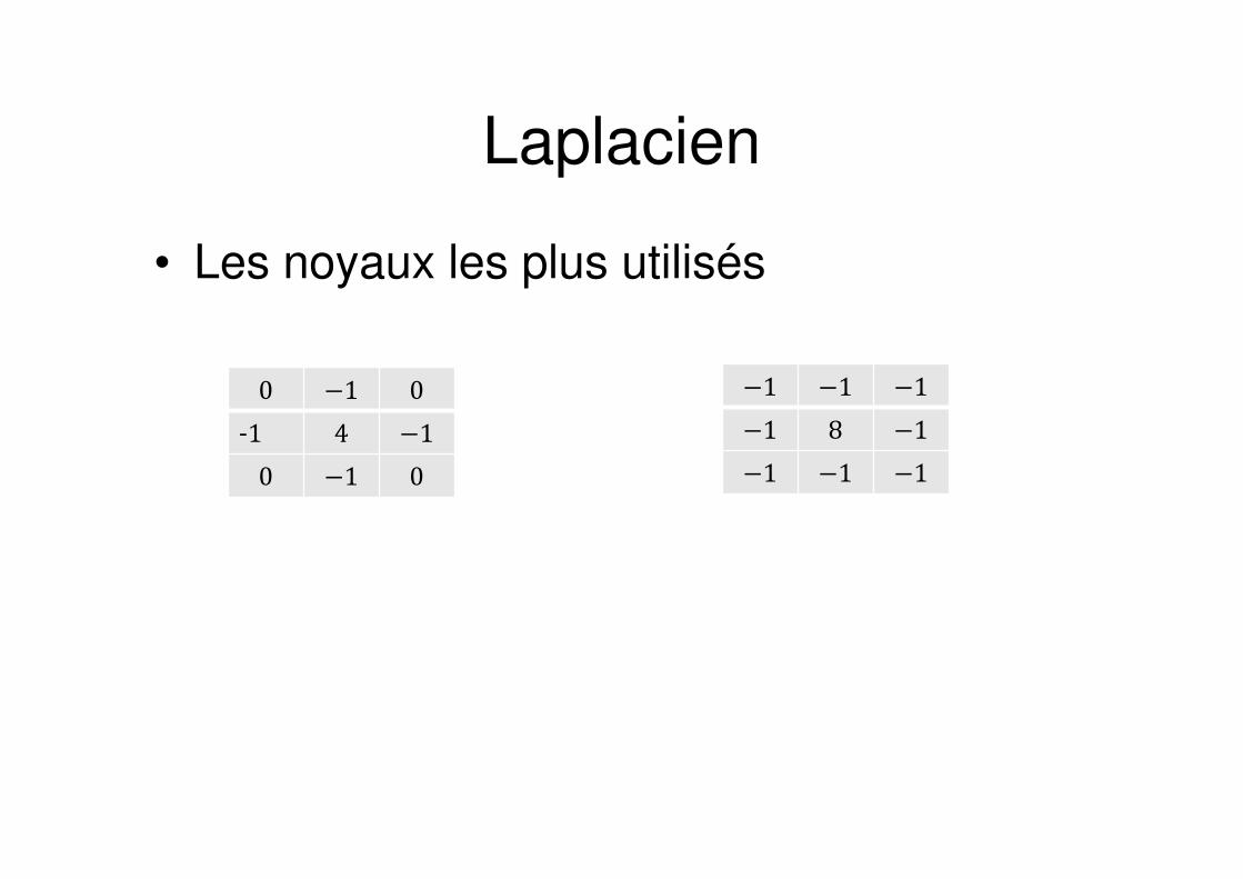
Laplacien
• Les noyaux les plus utilisés
0 −1 0-1 4 −10 −1 0
−1 −1 −1−1 8 −1−1 −1 −1
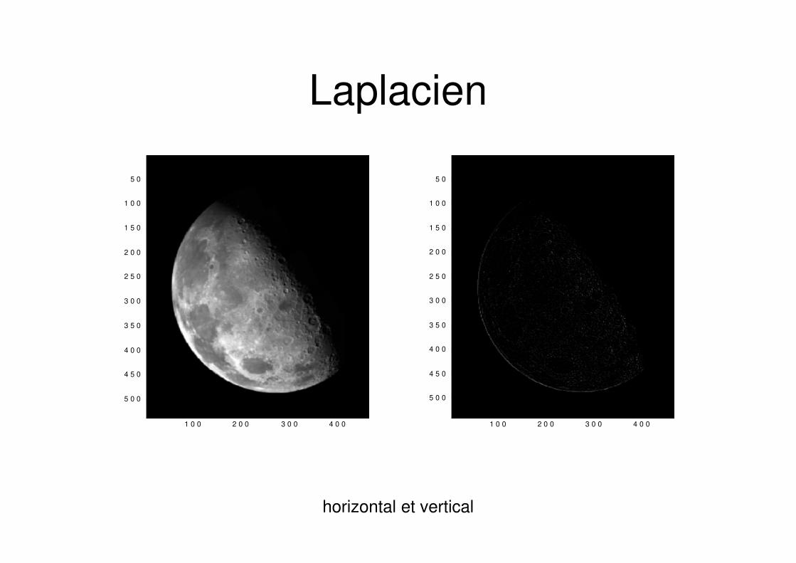
Laplacien
1 0 0 2 0 0 3 0 0 4 0 0
5 0
1 0 0
1 5 0
2 0 0
2 5 0
3 0 0
3 5 0
4 0 0
4 5 0
5 0 0
1 0 0 2 0 0 3 0 0 4 0 0
5 0
1 0 0
1 5 0
2 0 0
2 5 0
3 0 0
3 5 0
4 0 0
4 5 0
5 0 0
horizontal et vertical

Laplacien
1 0 0 2 0 0 3 0 0 4 0 0
5 0
1 0 0
1 5 0
2 0 0
2 5 0
3 0 0
3 5 0
4 0 0
4 5 0
5 0 0
1 0 0 2 0 0 3 0 0 4 0 0
5 0
1 0 0
1 5 0
2 0 0
2 5 0
3 0 0
3 5 0
4 0 0
4 5 0
5 0 0
horizontal, vertical et diagonal

Amélioration de la netteté
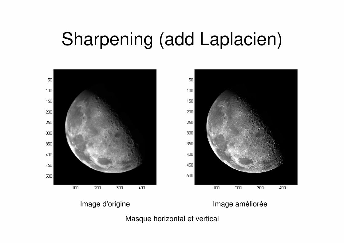
Sharpening (add Laplacien)
Image d'origine Image améliorée
Masque horizontal et vertical

Sharpening (add Laplacien)
Image d'origine Image améliorée
Masque horizontal, vertical et diagonal

Sharpening spatial filter
Image d'origine Image améliorée
Masque horizontal et vertical

Laplacien
1 0 0 2 0 0 3 0 0 4 0 0 5 0 0
5 0
1 0 0
1 5 0
2 0 0
2 5 0
3 0 0
3 5 0
4 0 0
4 5 0
5 0 0
1 0 0 2 0 0 3 0 0 4 0 0 5 0 0
5 0
1 0 0
1 5 0
2 0 0
2 5 0
3 0 0
3 5 0
4 0 0
4 5 0
5 0 0
horizontal, vertical et diagonal
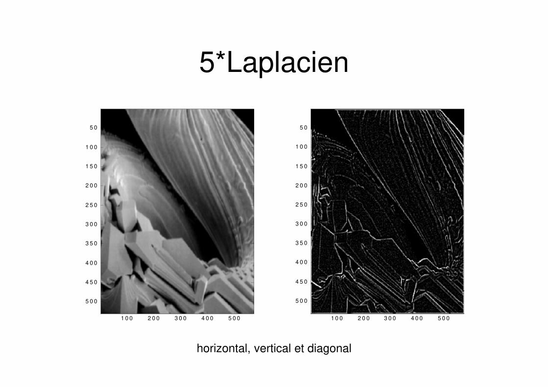
5*Laplacien
1 0 0 2 0 0 3 0 0 4 0 0 5 0 0
5 0
1 0 0
1 5 0
2 0 0
2 5 0
3 0 0
3 5 0
4 0 0
4 5 0
5 0 0
1 0 0 2 0 0 3 0 0 4 0 0 5 0 0
5 0
1 0 0
1 5 0
2 0 0
2 5 0
3 0 0
3 5 0
4 0 0
4 5 0
5 0 0
horizontal, vertical et diagonal

Sharpening spatial filter
Image d'origine Image améliorée
Masque horizontal, vertical et diagonal

Sharpening spatial filter
1 0 0 2 0 0 3 0 0 4 0 0 5 0 0
5 0
1 0 0
1 5 0
2 0 0
2 5 0
3 0 0
3 5 0
4 0 0
4 5 0
1 0 0 2 0 0 3 0 0 4 0 0 5 0 0
5 0
1 0 0
1 5 0
2 0 0
2 5 0
3 0 0
3 5 0
4 0 0
4 5 0
Masque horizontal, vertical et diagonal

Image en couleur
• Un pixel est représenté par
– un octet pour une image en nuance d gris
– 3 octets pour une image en couleur (24 bits/pixel)
• Les octets d’un pixel en couleur représentent les niveaux rouge, vert et bleu
• La luminance du pixel peut se calculer par la relation
� = �. z� + �. |�� + �. xx�255 255 0 0 255 255 255 0 255
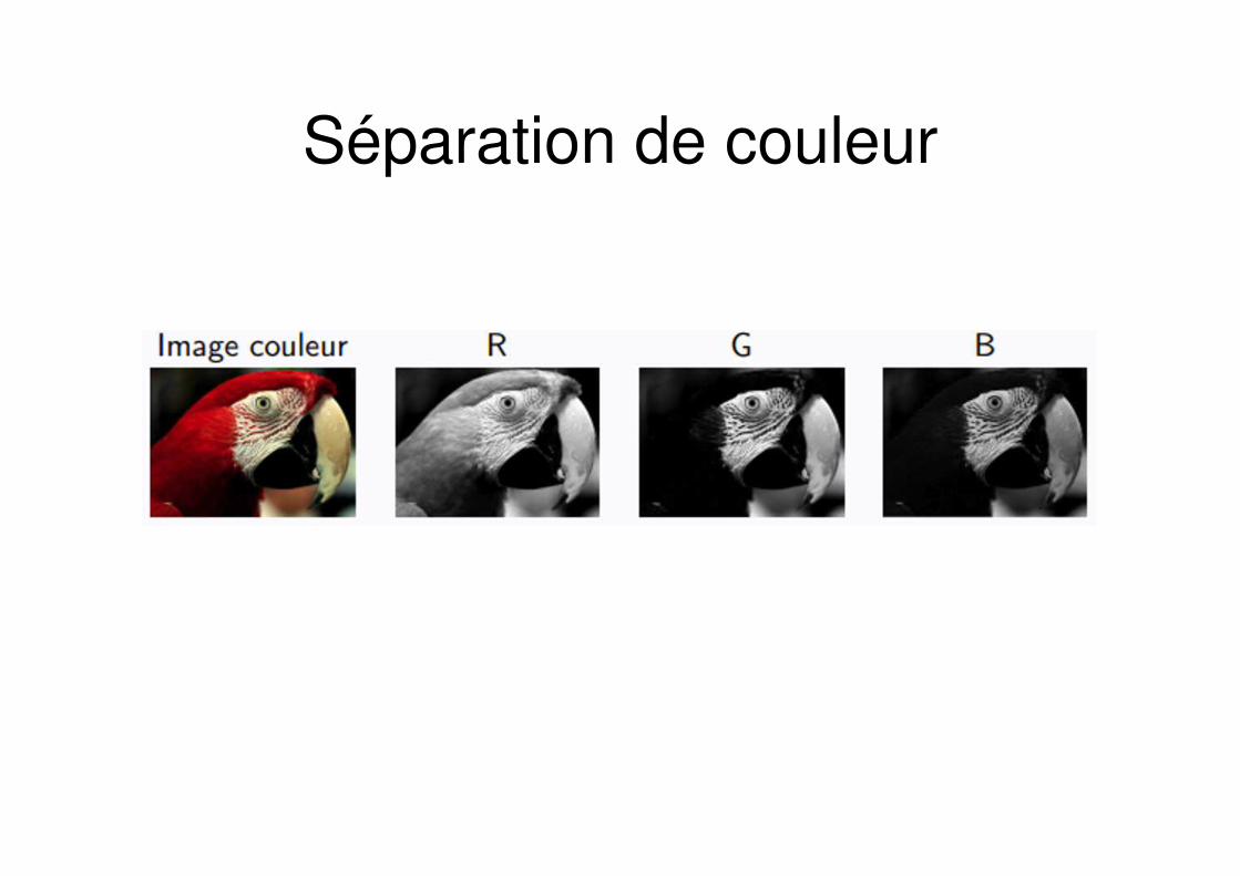
Séparation de couleur

Espace RGB
• Espace de couleur en RGB ne donne pas des couleurs
pures.
• La distance perceptuelle entre deux couleurs ne
coïncide pas avec a distance dans l’espace RGB
• D’autre espace couleur sont utilisés:
– HSV (Hue :Teinte, Saturation, Value : luminance)
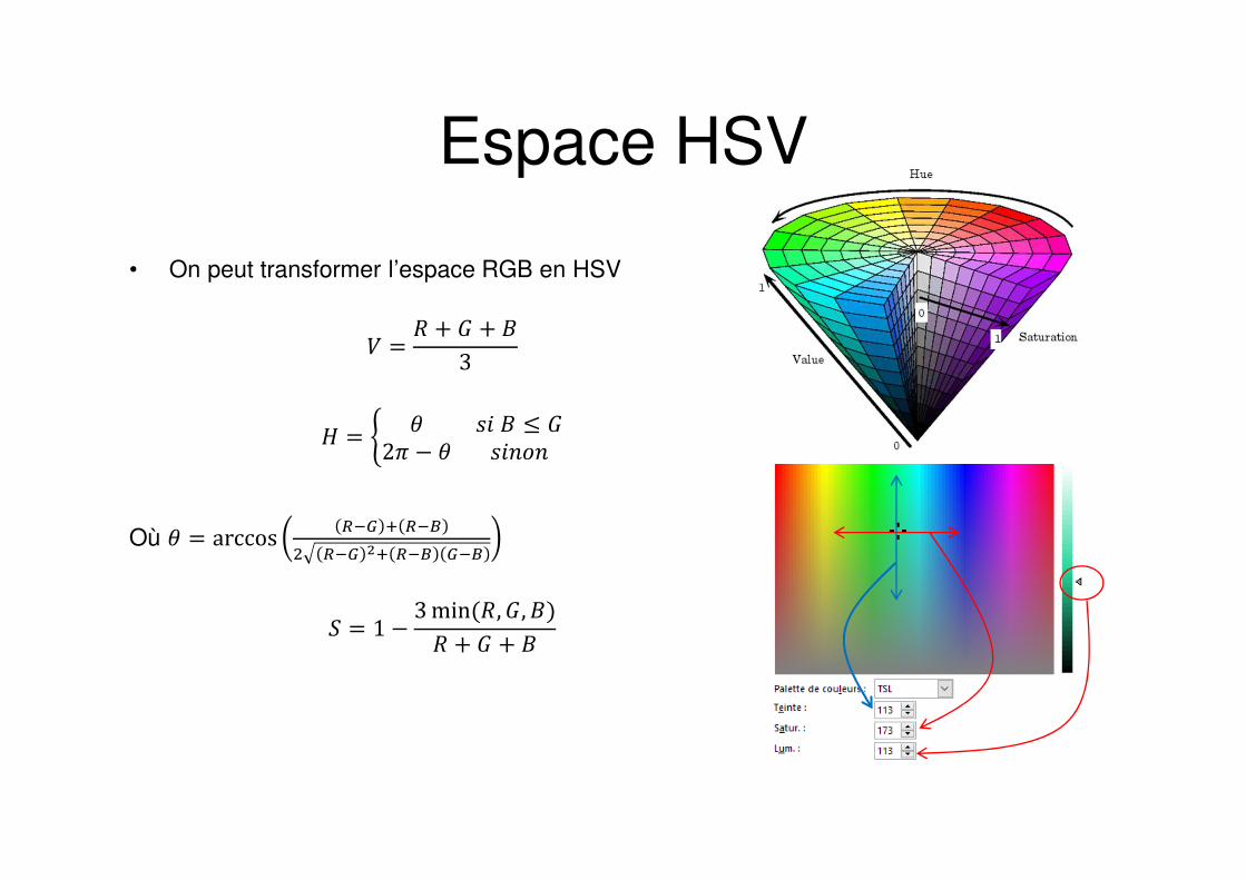
Espace HSV
• On peut transformer l’espace RGB en HSV
� = � + � + �3� = � , >� � ≤ �2� − , >�T�T
Où , = arccos �X_ � �X�$ �X_ �� �X� _X�c
d = 1 − 3 min(�, �, �)� + � + �
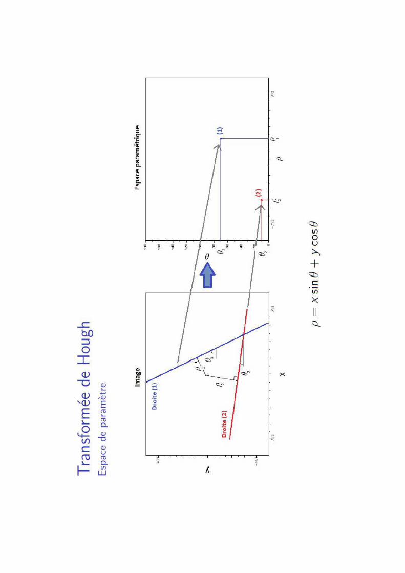
Reconnaissance de
forme La reconnaissance de droite dans une image :
Transformée de Hough

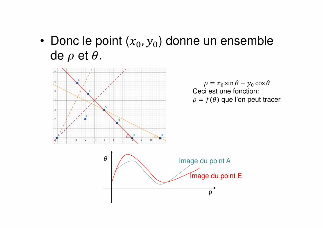
• Donc le point (��, ��) donne un ensemble de � et ,.
ρ
,
� = �� sin , + �� cos ,Ceci est une fonction: � = �(,) que l’on peut tracer
Image du point A
Image du point E

Images des points alignés
Les images des points alignés se croisent sur le même point (��, ,�)
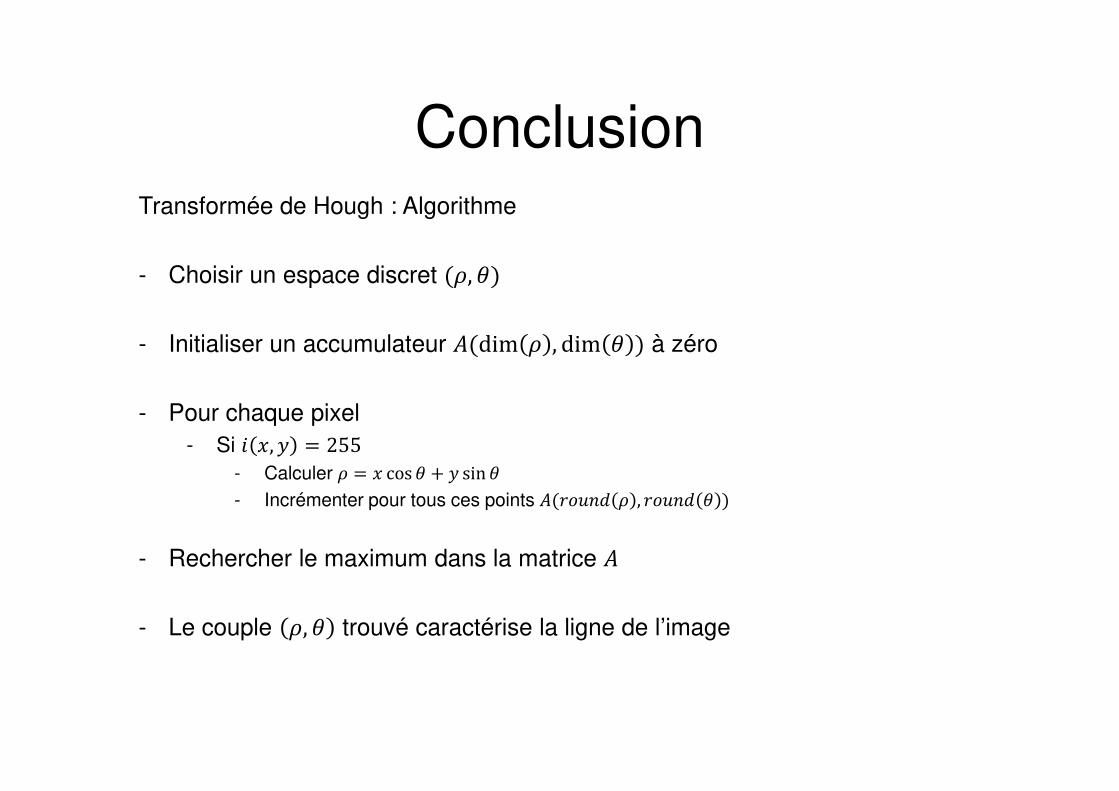
ConclusionTransformée de Hough : Algorithme
- Choisir un espace discret (�, ,)- Initialiser un accumulateur �(dim � , dim , ) à zéro
- Pour chaque pixel
- Si � �, � = 255- Calculer � = � cos , + � sin ,- Incrémenter pour tous ces points �(?��T � , ?��T , )
- Rechercher le maximum dans la matrice �- Le couple �, , trouvé caractérise la ligne de l’image
Related Documents