Color Quantization Luc Brun ´ Equipe Traitement Num´ erique des Images -Laboratoire LERI Universit´ e de Reims Champagne Ardenne - France E-Mail: [email protected] Alain Tr´ emeau ´ Equipe Ing´ enierie de la Vision - Laboratoire LIGIV Universit´ e Jean Monnet de Saint-Etienne - France E-Mail: [email protected]

Welcome message from author
This document is posted to help you gain knowledge. Please leave a comment to let me know what you think about it! Share it to your friends and learn new things together.
Transcript
Color Quantization
Luc Brun
Equipe Traitement Numerique des Images -Laboratoire LERI
Universite de Reims Champagne Ardenne - France
E-Mail: [email protected]
Alain Tremeau
Equipe Ingenierie de la Vision - Laboratoire LIGIV
Universite Jean Monnet de Saint-Etienne - France
E-Mail: [email protected]

2
Contents
1 Color Quantization 5
1.1 Introduction . . . . . . . . . . . . . . . . . . . . . . . . . . . . . . . . . . . . . 51.2 Image independent quantization methods . . . . . . . . . . . . . . . . . . . . 61.3 Preprocessing steps of image dependent quantization methods . . . . . . . . . 7
1.3.1 Pre-quantization . . . . . . . . . . . . . . . . . . . . . . . . . . . . . . 81.3.2 Histogram calculation . . . . . . . . . . . . . . . . . . . . . . . . . . . 8
1.4 Clustering Methods . . . . . . . . . . . . . . . . . . . . . . . . . . . . . . . . . 91.4.1 3x1D quantization methods . . . . . . . . . . . . . . . . . . . . . . . . 121.4.2 3D Splitting methods . . . . . . . . . . . . . . . . . . . . . . . . . . . 131.4.3 Grouping methods . . . . . . . . . . . . . . . . . . . . . . . . . . . . . 171.4.4 Merge methods . . . . . . . . . . . . . . . . . . . . . . . . . . . . . . . 201.4.5 Popularity methods . . . . . . . . . . . . . . . . . . . . . . . . . . . . 21
1.5 Quantization algorithms based on weighted errors . . . . . . . . . . . . . . . . 221.6 Post clustering methods . . . . . . . . . . . . . . . . . . . . . . . . . . . . . . 26
1.6.1 The LBG and k-means algorithms . . . . . . . . . . . . . . . . . . . . 261.6.2 The NeuQuant Neural-Net image quantization algorithm . . . . . . . 271.6.3 The local k-means algorithm. . . . . . . . . . . . . . . . . . . . . . . . 27
1.7 Mapping methods . . . . . . . . . . . . . . . . . . . . . . . . . . . . . . . . . 281.7.1 Improvements of the trivial inverse colormap method . . . . . . . . . . 281.7.2 Inverse colormap algorithms devoted to a specific quantization method 291.7.3 Inverse colormap operations using k − d trees . . . . . . . . . . . . . . 291.7.4 The locally sorted search algorithm . . . . . . . . . . . . . . . . . . . . 301.7.5 Inverse colormap operation using a 3D Voronoı diagram . . . . . . . . 311.7.6 Inverse colormap operation by a 2D Voronoı diagram . . . . . . . . . . 31
1.8 Dithering methods . . . . . . . . . . . . . . . . . . . . . . . . . . . . . . . . . 331.8.1 The Error diffusion methods . . . . . . . . . . . . . . . . . . . . . . . 331.8.2 The Ordered dither methods . . . . . . . . . . . . . . . . . . . . . . . 351.8.3 Vector dither methods . . . . . . . . . . . . . . . . . . . . . . . . . . . 351.8.4 Joint quantization and dithering methods . . . . . . . . . . . . . . . . 36
1.9 Conclusion and perspectives . . . . . . . . . . . . . . . . . . . . . . . . . . . . 371.10 List of Figures . . . . . . . . . . . . . . . . . . . . . . . . . . . . . . . . . . . 44
3

4 CONTENTS
Chapter 1
Color Quantization
1.1 Introduction
Color image quantization is used to reduce the number of colors of a digital image with aminimal visual distortion. Color quantization can also be defined as a lossy image compres-sion operation. Until lately, quantization was used to reproduce 24 bit images on graphicshardware with a limited number of simultaneous colors (e.g frame buffer displays with 4 or8 bit colormaps). Even though 24 bit graphics hardware is becoming more common, colorquantization still maintains its practical value. It lessens space requirements for storage ofimage data and reduces transmission band width requirements in multimedia applications.
Given a color image I, let us denote by CI the set of its colors and by M the cardinalityof CI . The quantization of I into K colors, with K < M (and usually K << M) consists inselecting a set of K representative colors and replacing the color of each pixel of the originalimage by a suitable representative color.
Since first applications of quantization were used to display full color images on low-costcolor output devices, quantization algorithms had from the beginning to face to two con-straints. On one hand, the quantized image must be computed at the time the image isdisplayed. This makes computational efficiency of critical importance. On the other hand,the visual distortion between the original image and the reproduced one has to be as smallas possible. The trade off between computational times and quantized image quality is appli-cation dependent and many quantization methods have been designed according to variousconstraints on this trade off.
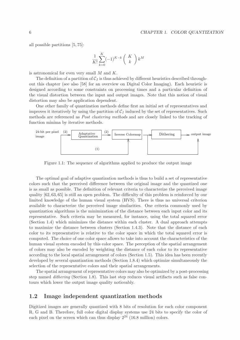
One straightforward way to obtain quantized images with low computational times con-sists to use a preselected set of representative colors [29, 49]. Such methods, described inSection 1.2, are referenced as image independent quantization methods (see also arrow (1) inFigure 1.1). Quantized images with higher quality are generally obtained by building the setof representative colors according to the color distribution of the input image. Such methodsare called Adaptative quantization methods or Image dependent quantization methods (arrows(2) in Figure 1.1).
Given an input image and a set of representative colors, the mapping of each color ofthe original image to one representative is performed by the Inverse colormap operation (Fig-ure 1.1 and Section 1.7). Since each color of the original image is mapped onto a representativecolor, the definition of the set of representative colors induces a partition of the image colorset CI . The notions of color set partition and representative colors are thus closely linkedand many quantization methods define first a partition of CI into a set of clusters and inducefrom it a set of representative colors. The brute force of enumerating all possible partitionsof the set CI with M colors into K subsets is out of the question here, since the number of
5
6 CHAPTER 1. COLOR QUANTIZATION
all possible partitions [5, 75]:
1
K!
K∑
k=0
(−1)K−k
(
Kk
)
kM
is astronomical for even very small M and K.
The definition of a partition of CI is thus achieved by different heuristics described through-out this chapter (see also [58] for an overview on Digital Color Imaging). Each heuristic isdesigned according to some constraints on processing times and a particular definition ofthe visual distortion between the input and output images. Note that this notion of visualdistortion may also be application dependent.
One other family of quantization methods define first an initial set of representatives andimproves it iteratively by using the partition of CI induced by the set of representatives. Suchmethods are referenced as Post clustering methods and are closely linked to the tracking offunction minima by iterative methods.
(2) (2)
(1)
AdaptativeQuantization
Inverse Colormap Dithering24-bit per pixel
imageoutput image
Figure 1.1: The sequence of algorithms applied to produce the output image
The optimal goal of adaptive quantization methods is thus to build a set of representativecolors such that the perceived difference between the original image and the quantized oneis as small as possible. The definition of relevant criteria to characterize the perceived imagequality [62, 63, 65] is still an open problem. The difficulty of this problem is reinforced by ourlimited knowledge of the human visual system (HVS). There is thus no universal criterionavailable to characterize the perceived image similarities. One criteria commonly used byquantization algorithms is the minimization of the distance between each input color and itsrepresentative. Such criteria may be measured, for instance, using the total squared error(Section 1.4) which minimizes the distance within each cluster. A dual approach attemptsto maximize the distance between clusters (Section 1.4.3). Note that the distance of eachcolor to its representative is relative to the color space in which the total squared error iscomputed. The choice of one color space allows to take into account the characteristics of thehuman visual system encoded by this color space. The perception of the spatial arrangementof colors may also be encoded by weighting the distance of each color to its representativeaccording to the local spatial arrangement of colors (Section 1.5). This idea has been recentlydeveloped by several quantization methods (Section 1.8.4) which optimize simultaneously theselection of the representative colors and their spatial arrangements.
The spatial arrangement of representative colors may also be optimized by a post-processingstep named dithering (Section 1.8). This last step reduces visual artifacts such as false con-tours which lower the output image quality noticeably.
1.2 Image independent quantization methods
Digitized images are generally quantized with 8 bits of resolution for each color componentR, G and B. Therefore, full color digital display systems use 24 bits to specify the color ofeach pixel on the screen which can thus display 224 (16.8 million) colors.
1.3. PREPROCESSING STEPS OF IMAGE DEPENDENT QUANTIZATION METHODS 7
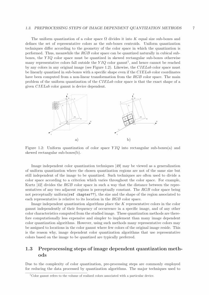
The uniform quantization of a color space Ω divides it into K equal size sub-boxes anddefines the set of representative colors as the sub-boxes centroids. Uniform quantizationtechniques differ according to the geometry of the color space in which the quantization isperformed. Thus, meanwhile the RGB color space can be quantized naturally in cubical sub-boxes, the Y IQ color space must be quantized in skewed rectangular sub-boxes otherwisemany representative colors fall outside the Y IQ color gamut1, and hence cannot be reachedby any colors in any original image (see Figure 1.2). Likewise, the CIELab color space mustbe linearly quantized in sub-boxes with a specific shape even if the CIELab color coordinateshave been computed from a non-linear transformation from the RGB color space. The mainproblem of the uniform quantization of the CIELab color space is that the exact shape of agiven CIELab color gamut is device dependent.
R
B
CW
G
M
1.0
1.0
1.0(0 0 0)
B
I
Q
Y
Y
R
B
CW
G
M
1.0
1.0
1.0(0 0 0)
B
I
Q
Y
Y
a) b)
Figure 1.2: Uniform quantization of color space Y IQ into rectangular sub-boxes(a) andskewed rectangular sub-boxes(b).
Image independent color quantization techniques [49] may be viewed as a generalizationof uniform quantization where the chosen quantization regions are not of the same size butstill independent of the image to be quantized. Such techniques are often used to divide acolor space according to a criterion which varies throughout the color space. For example,Kurtz [42] divides the RGB color space in such a way that the distance between the repre-sentatives of any two adjacent regions is perceptually constant. The RGB color space beingnot perceptually uniform(ref chapter??), the size and the shape of the region associated toeach representative is relative to its location in the RGB color space.
Image independent quantization algorithms place the K representative colors in the colorgamut independently of their frequency of occurrence in a specific image, and of any othercolor characteristics computed from the studied image. These quantization methods are there-fore computationally less expensive and simpler to implement than many image dependentcolor quantization algorithms. However, using such methods many representative colors maybe assigned to locations in the color gamut where few colors of the original image reside. Thisis the reason why, image dependent color quantization algorithms that use representativecolors based on the image to be quantized are typically preferred.
1.3 Preprocessing steps of image dependent quantization meth-
ods
Due to the complexity of color quantization, pre-processing steps are commonly employedfor reducing the data processed by quantization algorithms. The major techniques used to
1Color gamut refers to the volume of realized colors associated with a particular device.
8 CHAPTER 1. COLOR QUANTIZATION
reduce the data are the pre-quantization which reduces the range of each coordinate in thecolor space and the histogram calculation which allows to manage more efficiently the imagecolor set.
1.3.1 Pre-quantization
The “pre-quantization”, in 5 bits for each color component, is commonly used by many algo-rithms as a basic step for the quantization process. The main purpose of this pre-quantizationis to enables a trade off between quantizer complexity and image quality. Indeed, Fletcher [25]has shown that this initial step noticeably reduces the memory and computational time re-quirements of quantization algorithms. Other approaches have exploited this advantage fur-ther by using a “pre-quantization” in 4 bits of resolution for each color component [37], oreven in 3 bits of resolution for each color component [32].
The main drawback of these approaches is that they do not take into account the non-uniformity of human visual system to perceived color differences. Indeed, while this pre-quantization may produce non-noticeable degradations in high frequency areas, it can atthe same time produce visible degradations in low frequency areas or at the border of con-tours [61, 63]. Balasubramanian [8, 10] proposed to base the pre-quantization step on anactivity measure defined from the spatial arrangement of colors (Section 1.5). However, inthis case the computational cost of the pre-quantization step is no longer negligible and theadditional computation time induced by this step has to be compared to the computationtime of the quantization algorithm without pre-quantization.
A last approach proposed by Kurz [42] estimates the color distribution of an image andits relative importance by examining the pixels at a fixed number of random locations. Kurzproposes to use 1024 random locations for a 512×512 image. Randomizing the pixel locationsavoids repeated selection of certain colors in the color set, particularly in images with periodicpattern(s).
1.3.2 Histogram calculation
The first pre-processing step of an image quantization algorithm generally consists of his-togram computation of the image color set i.e., a functionH is computed such thatH(R,G,B)is equal to the number of pixels of the image whose color is equal to (R,G,B). Using the RGBcolor space, one straightforward implementation of this function is to allocate a 256×256×256array. Given this array, the computation of the histogram is performed by incrementing thecorresponding entry of each pixel’s color. However, this method has several disadvantages:First, the size of the image being quantized is generally much smaller than the size of thefull histogram indicated above and many entries of the histogram are set to 0 or very smallvalues. This last property may induce some unwanted behavior for some algorithms. Forexample, the determination of the most occurring color, may “loose” important colors if theyare encoded in the histogram by a set of adjacent entries with low frequencies. Secondly, thisencoding requires the storage of 2563 indexes. Encoding each entry of the array by 2 bytes,leads to a storage requirement of 32Mbytes. Finally, many quantization algorithms usingother color spaces than RGB, the allocation of an array enclosing the color gamut of thesecolor spaces reinforce the problems linked with the sparse property of the histogram and itsstorage requirements.
One partial solution to this problem proposed by Heckbert [35] consists to remove the 3least significant bits of each component in order to store the histogram in an array of size32× 32× 32. This solution reduces both the memory requirements and the problems inducedby the sparseness of the histogram. However, the removal of the 3 least significant bits isequivalent to a pre-quantization which may induce a visible loss of image quality when the
1.4. CLUSTERING METHODS 9
output image is quantized into large number of colors such as 256 (Section 1.3.1). Moreover,using a color space other than RGB, one has to define the box enclosing the reduced RGBcolor space. According to the color space this box may remain large beside the uniformquantization step.
One simple encoding of the histogram allocates an array whose size is equal to the numberof different colors contained in the image. Each entry of this array is defined as a couple offields encoding respectively a color contained in the image and the number of image’s pixelsof the corresponding color. This array may be initialized using a hash table and is widelyused by tree-structured vector quantization algorithms (Section 1.4.2). Note that this lastdata structure is not designed to facilitate the determination of the number of image’s pixelswhose color is equal to a given value but rather to traverse the color space or a part of it inorder to compute some of its statistical parameters such the mean or the variance.
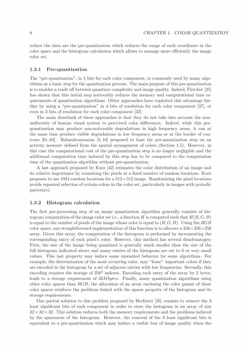
Xiang [77] proposes an encoding of the RGB histogram based on a 2D array of listsindexed by the R and G color coordinates. During the traversal of the image each pixel withcolor (R,G,B) induces an update of the list of B values stored in the entry (R,G) of thearray. If the component B is not present in the list, a new node is inserted with a colorcomponent storing the B value and a frequency field initialized to 1. If B is already presentin the list the frequency of the corresponding node is incremented. Each list is doubly linkedand sorted in ascending order according to the blue field (see Figure 1.3(a)). Therefore, if Sdenotes the mean size of the blue lists, the retrieval of the number of pixels whose color isequal to a given (R,G,B) triplet requires O(S2 ) comparisons. Balasubramanian [10] improvesthe search by storing in each entry of the (R,G) array a binary tree ordered according to theblue values(see Figure 1.3(b)). The computational time required to retrieve a given (R,G,B)is then reduced to O(log(S)).
2, f1
6, f2
8, f3
R
G
15, f5
10, f4
R
G
6, f2
8, f42, f3
15, f5
10, f1
a) b)
Figure 1.3: The histograms of Xiang [77] a) and Balasubramanian [10] b)
1.4 Clustering Methods
Clustering techniques perform a partition of the color space according to some criteria. Suchcriteria do not attempt to optimize the spatial arrangement of representatives which may beimproved by a dithering algorithm applied as a correcting step (Section 1.8). The input dataof such algorithms are thus the image color set CI and the frequency of occurrence of eachcolor c in the image: f(c).
As anticipated in Section 1.1, quantization algorithms may be decomposed in two mainfamilies: post-clustering methods which define a set of K representatives improved by aniterative scheme and pre-clustering methods which define a partition of CI into K clustersand associate one representative to each cluster. Clustering quantization methods belongto the latter family. Each cluster (Ci)i∈1,...,K of the partition may be characterized bystatistical properties such as its mean, its variance along one coordinate axis or its covariance
10 CHAPTER 1. COLOR QUANTIZATION
matrix. All these parameters may be deduced from the following quantities:
card(C) =∑
c∈C f(c)M1(C) =
∑
c∈C f(c)cM2(C) =
∑
c∈C f(c)(c21, c22, c
23)
R2(C) =∑
c∈C f(c)c • ct
(1.1)
where (c2i )i∈1,2,3 denotes the squared value of the ith coordinate of the vector c and f(c)denotes the number of pixels of the original image whose color is c.
The quantities card(C), M1(C) and M2(C) are respectively called the cardinal, the firstand the second cumulative moments of the cluster. Note that, card(C) is a real number, whileM1(C) and M2(C) are 3D vectors. The quantity R2(C) is a 3 × 3 matrix whose diagonal isequal to M2(C).
The main advantage of the above quantities is that they can be efficiently updated duringthe merge or split operations performed by clustering quantization algorithms. For exampleif two clusters C1 and C2 must be merged, the cardinal of the merged cluster is equal tocard(C1∪C2) = card(C1)+card(C2). The same relation holds forM1, M2 and R2. Conversely,if one cluster C is split into two sub clusters C1 and C2 and if both the statistics of C and C1
are known, the statistics of C2 may be deduced from the ones of C and C1. For example, thecardinal of C2 is defined as card(C)− card(C1). The mean, the variances and the covariancematrix of one cluster may be deduced from the cardinal, the moments and the matrix R2 bythe following formula:
µ = M1(C)card(C)
vari = M2(C)icard(C) − µ2
i ∀i ∈ 1, 2, 3
Cov = R2(C)card(C) − µ.µt
(1.2)
where vari and µi denote respectively the variance of cluster C along the coordinate axis Ωi
and the ith coordinate of the mean vector µ. The symbol Cov denotes the covariance matrixof the cluster.
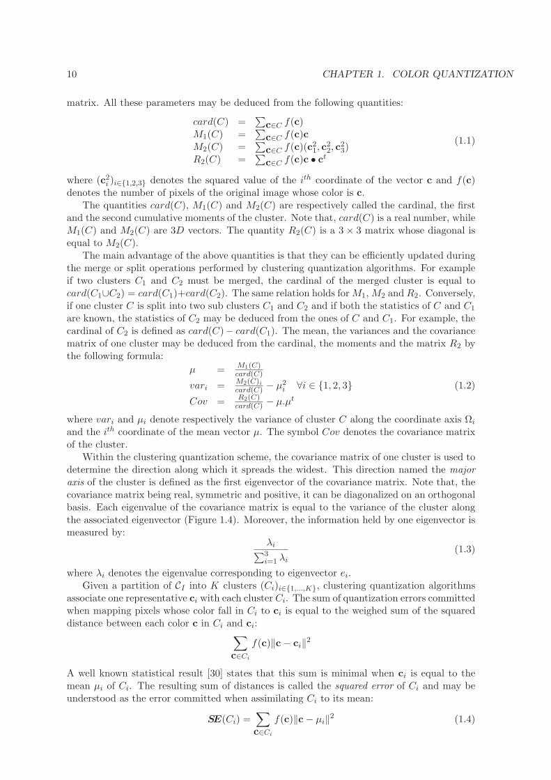
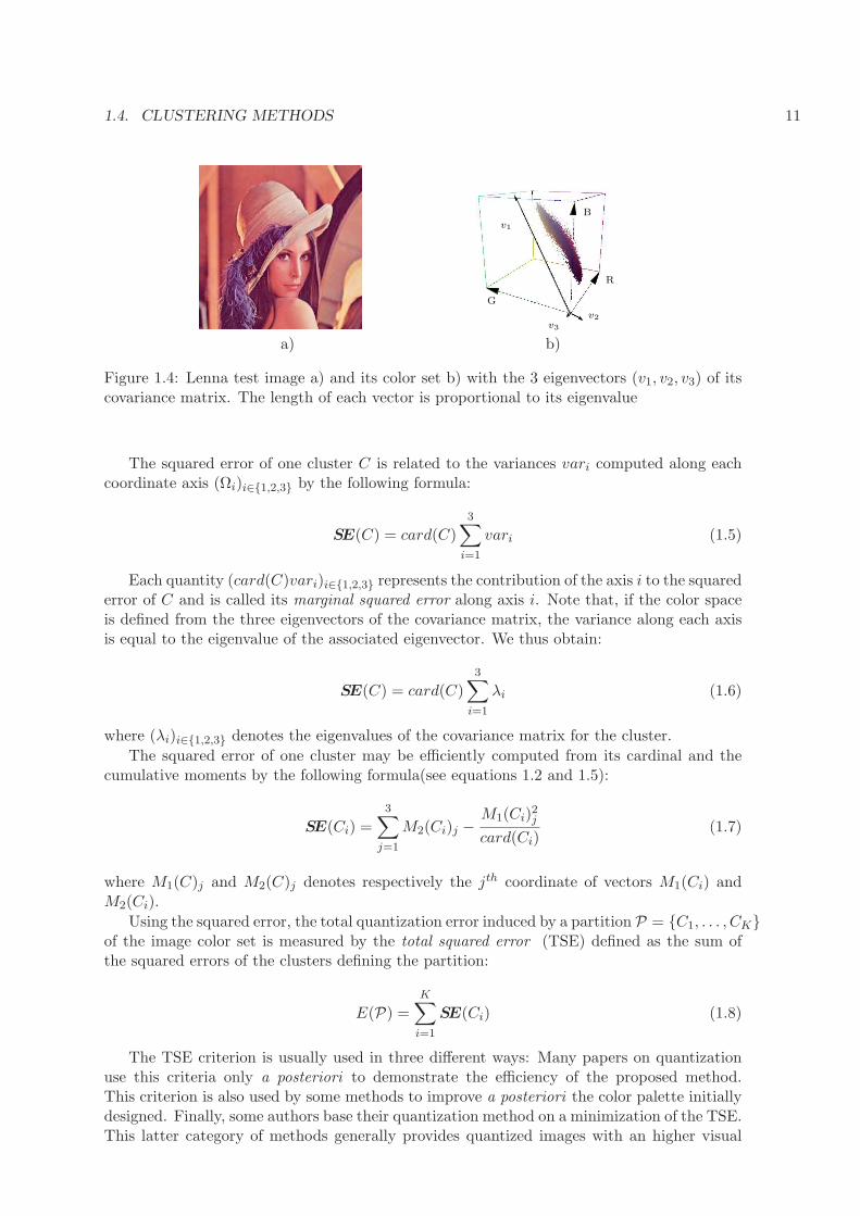
Within the clustering quantization scheme, the covariance matrix of one cluster is used todetermine the direction along which it spreads the widest. This direction named the majoraxis of the cluster is defined as the first eigenvector of the covariance matrix. Note that, thecovariance matrix being real, symmetric and positive, it can be diagonalized on an orthogonalbasis. Each eigenvalue of the covariance matrix is equal to the variance of the cluster alongthe associated eigenvector (Figure 1.4). Moreover, the information held by one eigenvector ismeasured by:
λi∑3
i=1 λi
(1.3)
where λi denotes the eigenvalue corresponding to eigenvector ei.Given a partition of CI into K clusters (Ci)i∈1,...,K, clustering quantization algorithms
associate one representative ci with each cluster Ci. The sum of quantization errors committedwhen mapping pixels whose color fall in Ci to ci is equal to the weighed sum of the squareddistance between each color c in Ci and ci:
∑
c∈Ci
f(c)‖c− ci‖2
A well known statistical result [30] states that this sum is minimal when ci is equal to themean µi of Ci. The resulting sum of distances is called the squared error of Ci and may beunderstood as the error committed when assimilating Ci to its mean:
SE(Ci) =∑
c∈Ci
f(c)‖c− µi‖2 (1.4)
1.4. CLUSTERING METHODS 11
v2
v3
v1
R
B
G
a) b)
Figure 1.4: Lenna test image a) and its color set b) with the 3 eigenvectors (v1, v2, v3) of itscovariance matrix. The length of each vector is proportional to its eigenvalue
The squared error of one cluster C is related to the variances vari computed along eachcoordinate axis (Ωi)i∈1,2,3 by the following formula:
SE(C) = card(C)
3∑
i=1
vari (1.5)
Each quantity (card(C)vari)i∈1,2,3 represents the contribution of the axis i to the squarederror of C and is called its marginal squared error along axis i. Note that, if the color spaceis defined from the three eigenvectors of the covariance matrix, the variance along each axisis equal to the eigenvalue of the associated eigenvector. We thus obtain:
SE(C) = card(C)3
∑
i=1
λi (1.6)
where (λi)i∈1,2,3 denotes the eigenvalues of the covariance matrix for the cluster.
The squared error of one cluster may be efficiently computed from its cardinal and thecumulative moments by the following formula(see equations 1.2 and 1.5):
SE(Ci) =3
∑
j=1
M2(Ci)j −M1(Ci)
2j
card(Ci)(1.7)
where M1(C)j and M2(C)j denotes respectively the jth coordinate of vectors M1(Ci) andM2(Ci).
Using the squared error, the total quantization error induced by a partition P = C1, . . . , CKof the image color set is measured by the total squared error (TSE) defined as the sum ofthe squared errors of the clusters defining the partition:
E(P) =K∑
i=1
SE(Ci) (1.8)
The TSE criterion is usually used in three different ways: Many papers on quantizationuse this criteria only a posteriori to demonstrate the efficiency of the proposed method.This criterion is also used by some methods to improve a posteriori the color palette initiallydesigned. Finally, some authors base their quantization method on a minimization of the TSE.This latter category of methods generally provides quantized images with an higher visual
12 CHAPTER 1. COLOR QUANTIZATION
quality than the two previous ones. However, these algorithms are generally computationallyintensive.
The different heuristics used to cluster colors may be decomposed into four main families:The 3 × 1D splitting methods described in Section 1.4.1 use the optimal algorithms definedfor one dimensional data to perform scalar quantization along each coordinate axis. The 3Dsplitting methods splits the 3D image color set into a set of K clusters (Section 1.4.2). A largemajority of these methods split recursively the initial image color set by using a top-downscheme. Grouping methods, described in Section 1.4.3, use a bottom-up scheme by defininga set of empty clusters and aggregating each color of the image to one cluster. Finally, mergemethods described in Section 1.4.4 use a mixed approach by first splitting the image color setinto a set of clusters and then merging these clusters to obtain the K required clusters.
1.4.1 3x1D quantization methods
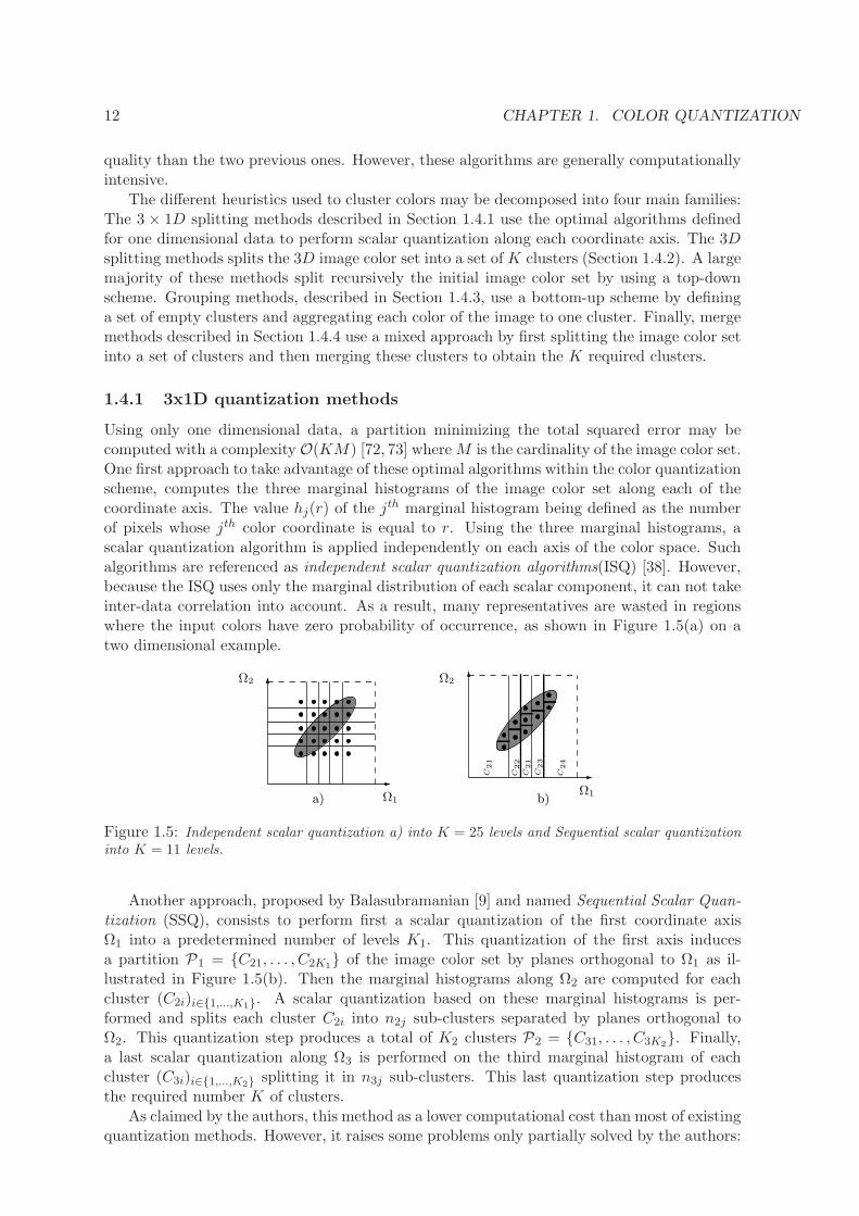
Using only one dimensional data, a partition minimizing the total squared error may becomputed with a complexity O(KM) [72, 73] whereM is the cardinality of the image color set.One first approach to take advantage of these optimal algorithms within the color quantizationscheme, computes the three marginal histograms of the image color set along each of thecoordinate axis. The value hj(r) of the jth marginal histogram being defined as the numberof pixels whose jth color coordinate is equal to r. Using the three marginal histograms, ascalar quantization algorithm is applied independently on each axis of the color space. Suchalgorithms are referenced as independent scalar quantization algorithms(ISQ) [38]. However,because the ISQ uses only the marginal distribution of each scalar component, it can not takeinter-data correlation into account. As a result, many representatives are wasted in regionswhere the input colors have zero probability of occurrence, as shown in Figure 1.5(a) on atwo dimensional example.
Ω1
Ω2
Ω1
C21
C23
C24
C21
C22
Ω2
a) b)
Figure 1.5: Independent scalar quantization a) into K = 25 levels and Sequential scalar quantizationinto K = 11 levels.
Another approach, proposed by Balasubramanian [9] and named Sequential Scalar Quan-tization (SSQ), consists to perform first a scalar quantization of the first coordinate axisΩ1 into a predetermined number of levels K1. This quantization of the first axis inducesa partition P1 = C21, . . . , C2K1
of the image color set by planes orthogonal to Ω1 as il-lustrated in Figure 1.5(b). Then the marginal histograms along Ω2 are computed for eachcluster (C2i)i∈1,...,K1. A scalar quantization based on these marginal histograms is per-formed and splits each cluster C2i into n2j sub-clusters separated by planes orthogonal toΩ2. This quantization step produces a total of K2 clusters P2 = C31, . . . , C3K2
. Finally,a last scalar quantization along Ω3 is performed on the third marginal histogram of eachcluster (C3i)i∈1,...,K2 splitting it in n3j sub-clusters. This last quantization step producesthe required number K of clusters.
As claimed by the authors, this method as a lower computational cost than most of existingquantization methods. However, it raises some problems only partially solved by the authors:
1.4. CLUSTERING METHODS 13
first, the final total squared error is dependent of the order in which the scalar quantizationsare performed (we have tacitly assumed that the Ωj are quantized in the order Ω1, Ω2, Ω3).The only means of finding the best order is to apply the quantization scheme on each of the3! = 6 possible orders. The authors address this problem by using the Y CrCb color space withone luminance (Y ) and two chrominance (Cr and Cb) axis. The authors perform first twoscalar quantization on the chrominance plane (Cr, Cb) followed by one scalar quantization ofthe luminance axis Y . This strategy being based on a fixed order of the quantizations maylead to sub-optimal results. The second problem raised by this method is the determinationof the number of quantization levels along each axis. In other words, what values of K1,K2, (n2j)j∈1,...,K1 and (n3j)j∈1,...,K2 should be picked to obtain the required number Kof final clusters. The authors estimate these quantities by using results from the asymptoticquantization theory. This theory being valid only for very large values of K, the authorsperform a preliminary quantization for some initial choice of K1 and K2 and correct theseinitial values as follows:
K1 = K01
(
d21
d2d3
)1
6
K2 = K02
(
d1d2d3
)1
6
with ∀j ∈ 1, 2, 3 dj =K∑
i=1
∑
c∈Ci
f(c)(cj − cji )
2 (1.9)
where K01 and K2
0 are the initial choice for K1 and K2 and d1, d2 and d3 denote the marginaltotal squared errors along each axis. Symbols (cj)j∈1,2,3 and (cji )j∈1,2,3 denote respectively
the jth coordinate of the color vector c and the ith representative ci.
1.4.2 3D Splitting methods
The 3D splitting methods have been intensively explored [8, 9, 12–14, 70–72, 74, 75] since 1982and the median cut method proposed by Heckbert [35]. These methods create a partition ofthe image color set into K clusters by a sequence of K − 1 split operations.
The initial image color set is thus split by a set of planes named cutting planes, each planebeing normal to one direction named the cutting axis. The location of the cutting plane alongthe cutting axis is named the cutting position. One justification for the use of planes withinthe 3D splitting scheme is provided by the inverse color map operation. Indeed, as mentionedin Section 1.4, given a set of representative colors c1, . . . , cK, an optimal mapping withrespect to the set of representatives maps each initial color to its closest representative. Thisoptimal mapping, induces a partition of the image color set by a 3D Voronoı diagram [60]defined by the representatives. Each cell of a 3D Voronoı diagram being delimited by a set ofplanes, the use of planes within the 3D splitting scheme does not induces a loss of generality.Note that, if each plane is assumed to be perpendicular to one of the coordinate axes eachcluster is an hyperbox.
As mentioned in Section 1.1, the set of all possible partitions into K clusters of the initialset of M data points is too large for an exhaustive enumeration. The 3D splitting schememust thus use a set of heuristics in order to restrict the set of possible partitions. Themain heuristics used by splitting quantization algorithms may be decomposed into four stepscommon to all algorithms of this family:
1. selection of a splitting strategy,
2. selection of the next cluster to be split,
3. selection of the cutting axis
4. selection of the cutting position.
14 CHAPTER 1. COLOR QUANTIZATION
The remaining of this section describes the main heuristics used at each of the above steps.The different choices performed by the methods described in this section are summarized inTable 1.1.
Splitting strategy
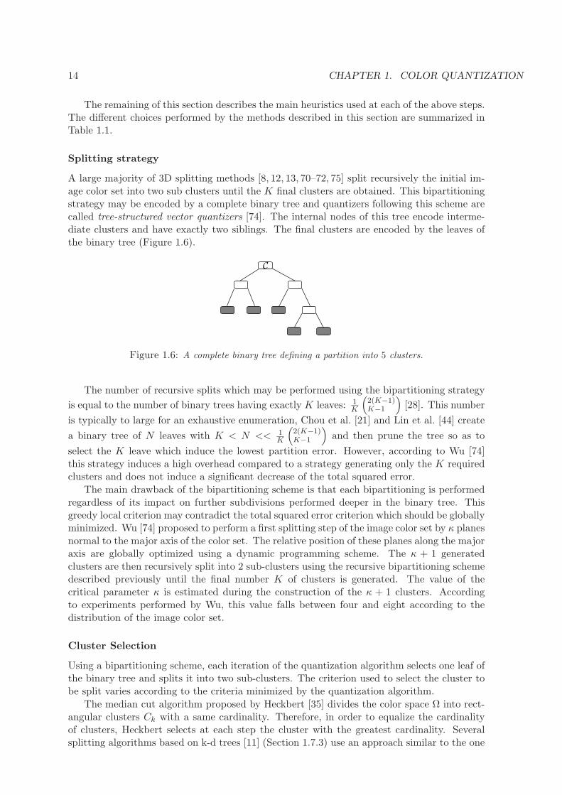
A large majority of 3D splitting methods [8, 12, 13, 70–72, 75] split recursively the initial im-age color set into two sub clusters until the K final clusters are obtained. This bipartitioningstrategy may be encoded by a complete binary tree and quantizers following this scheme arecalled tree-structured vector quantizers [74]. The internal nodes of this tree encode interme-diate clusters and have exactly two siblings. The final clusters are encoded by the leaves ofthe binary tree (Figure 1.6).
C
Figure 1.6: A complete binary tree defining a partition into 5 clusters.
The number of recursive splits which may be performed using the bipartitioning strategy
is equal to the number of binary trees having exactly K leaves: 1K
(
2(K−1)K−1
)
[28]. This number
is typically to large for an exhaustive enumeration, Chou et al. [21] and Lin et al. [44] create
a binary tree of N leaves with K < N << 1K
(
2(K−1)K−1
)
and then prune the tree so as to
select the K leave which induce the lowest partition error. However, according to Wu [74]this strategy induces a high overhead compared to a strategy generating only the K requiredclusters and does not induce a significant decrease of the total squared error.
The main drawback of the bipartitioning scheme is that each bipartitioning is performedregardless of its impact on further subdivisions performed deeper in the binary tree. Thisgreedy local criterion may contradict the total squared error criterion which should be globallyminimized. Wu [74] proposed to perform a first splitting step of the image color set by κ planesnormal to the major axis of the color set. The relative position of these planes along the majoraxis are globally optimized using a dynamic programming scheme. The κ + 1 generatedclusters are then recursively split into 2 sub-clusters using the recursive bipartitioning schemedescribed previously until the final number K of clusters is generated. The value of thecritical parameter κ is estimated during the construction of the κ + 1 clusters. Accordingto experiments performed by Wu, this value falls between four and eight according to thedistribution of the image color set.
Cluster Selection
Using a bipartitioning scheme, each iteration of the quantization algorithm selects one leaf ofthe binary tree and splits it into two sub-clusters. The criterion used to select the cluster tobe split varies according to the criteria minimized by the quantization algorithm.
The median cut algorithm proposed by Heckbert [35] divides the color space Ω into rect-angular clusters Ck with a same cardinality. Therefore, in order to equalize the cardinalityof clusters, Heckbert selects at each step the cluster with the greatest cardinality. Severalsplitting algorithms based on k-d trees [11] (Section 1.7.3) use an approach similar to the one
1.4. CLUSTERING METHODS 15
of Heckbert. These algorithms assign an approximately equal number of colors to all leavesof the tree. However, such a counterbalancing is not really adapted to image quantization.Indeed, there is no relevant justification to require that each cluster should contain a nearlyequal number of colors while ignoring how these colors are distributed in the color space [70].Using such method, a cluster with a large quantization error may not be split while a clustercontaining only one color (with a high occurrence frequency) may be subdivided instead.
A large majority [12–14, 70–72, 74, 75] of methods attempt to minimize the total squarederror. In order to obtain homogeneous clusters, Bouman [13] selects at each iteration thecluster whose data spread the widest along the splitting direction. Since Bouman splitsclusters along their major axis it selects the cluster whose principal eigenvalue is maximal.
Wan et al. [70] proposed to split at each step the cluster with the greatest squared error.The basic idea of this strategy is to split the cluster whose contribution to the TSE is thelargest. This strategy may be compared to the one of Bouman by writing the squared errorinto the base defined by the three eigenvectors of the covariance matrix:
SE(C) = card(C)3
∑
i=1
λi
The heuristic of Bouman may thus be understood as an approximation of the one of Wan ne-glecting the possible decrease of the variance along the directions defined by the two remainingeigenvectors.
One slightly different strategy has been proposed by Wu [75]. It consists to select at eachiteration the cluster whose bipartitioning yields the largest reduction of the total squarederror. Given a partition of the image color set into k clusters Pk = C1, . . . , Ck, the splittingof one cluster Ci into two sub clusters C1
i , C2i modifies the total squared error as follows:
E(Pk+1) = E(Pk) + SE(C1i ) + SE(C2
i )− SE(Ci) (1.10)
Note that, if both C1i and C2
i are non-empty, the value SE(C1i )+SE(C2
i )−SE(Ci) is strictlynegative. Therefore, the total squared error is a strictly decreasing function of the number ofsplit operations.
Wan’s heuristic may thus be considered as an approximation of the heuristic of Wu ne-glecting the squared errors of the two generated clusters. However, using the heuristic of Wu,each cluster must be split to estimate the decrease of the total squared error. According toexperiments performed by Wu [74], the difference between the two criteria in terms of finalquantization errors is marginal while the increase in computational costs is two folds for thesecond criteria. The selection at each iteration of the cluster with the greatest squared erroris thus a good compromised between the computational time and the final quantization error.
Cutting axis
Given the cluster Ci to be split one has to determine the normal and the location of the cuttingplane. Since the decrease of the total squared error after the split of Ci into C1
i and C2i is
equal to SE(C1i ) + SE(C2
i )− SE(Ci), the optimal cutting plane is the one which minimizesSE(C1
i ) + SE(C2i ). However, the freedom to place such a plane is still too enormous and we
need to fix the orientation of this plane to make the search feasible. Since the cutting of thecluster mainly decreases the variance along the cutting axis, one common heuristic consiststo select the cutting axis among the directions with a high variance (equation 1.5).
Heckbert [35] approximates the variance by enclosing the cluster into a rectangular box.The two sides of this box normal to the coordinate axis Ωi enclose the color vectors withminimum (resp. maximum) coordinates along Ωi. The spread of the data along each co-ordinate axis is then estimated by the length of the box along this axis and the box is cutperpendiculary to its longest axis.
16 CHAPTER 1. COLOR QUANTIZATION
Braquelaire et al. [14] compute the variance along each axis and split each cluster alongits coordinate axis with the greatest variance. This heuristic decreases the variance along thecoordinate axis which brings the major contribution to the squared error. One computationaladvantage of this heuristic is that the data set being split along three fixed directions(thecoordinate axis) the image color set may be pre-processed to optimize the determination ofthe cutting plane [14]. However, the coordinate axis with the greater variance is generally notthe axis along which the data set spread the widest. This direction is provided by the majoraxis of the cluster and the relation between the squared error of the cluster and the threeeigenvalues of the covariance matrix is provided by equation 1.6. Note that, if λ1 denotesthe principal eigenvalue of the major axis we have: ∀i ∈ 1, 2, 3 λ1 ≥ vari. Therefore, agreater decrease of the total squared error may be expected by cutting the cluster along itsmajor axis. This last heuristic is used by Wan [70, 71], Wu [74, 75] and Bouman [12, 13].
Cutting position
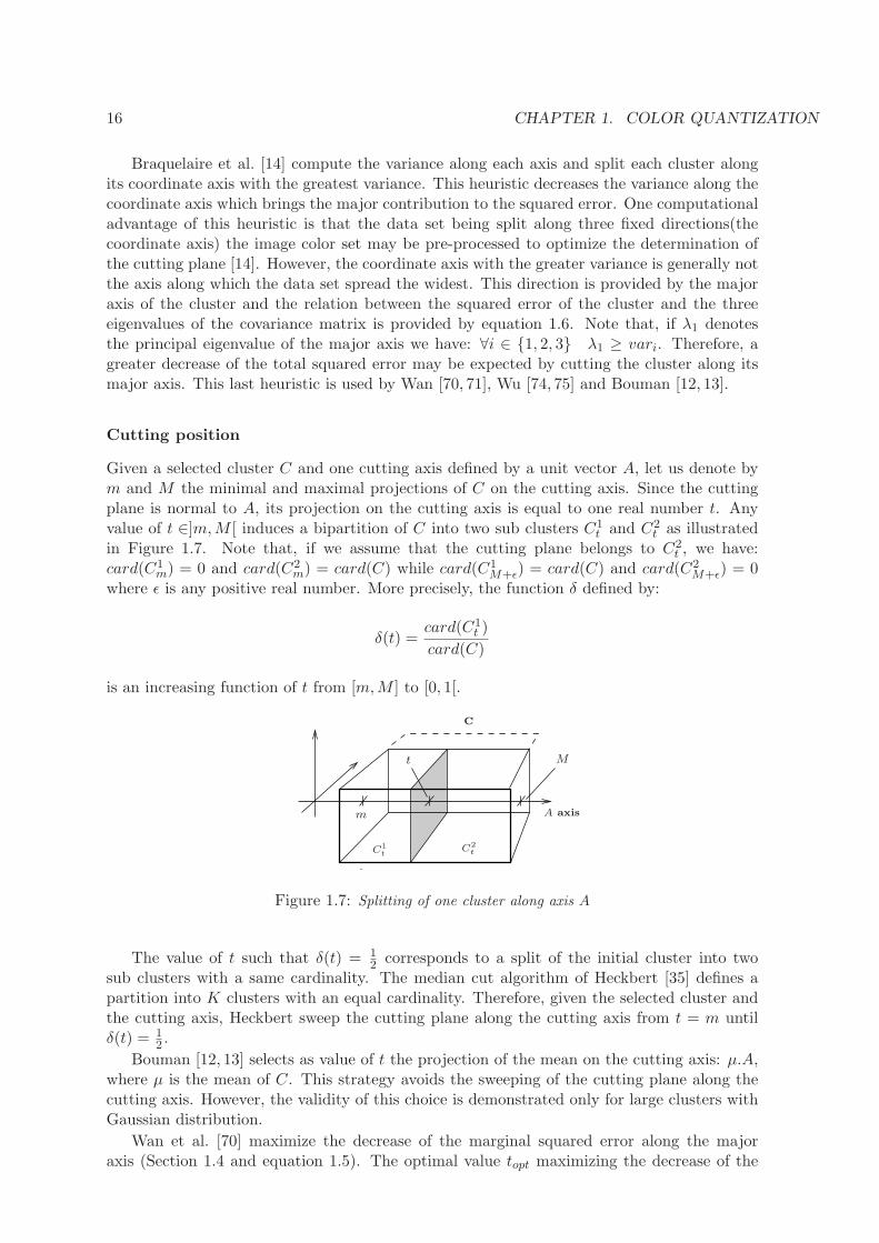
Given a selected cluster C and one cutting axis defined by a unit vector A, let us denote bym and M the minimal and maximal projections of C on the cutting axis. Since the cuttingplane is normal to A, its projection on the cutting axis is equal to one real number t. Anyvalue of t ∈]m,M [ induces a bipartition of C into two sub clusters C1
t and C2t as illustrated
in Figure 1.7. Note that, if we assume that the cutting plane belongs to C2t , we have:
card(C1m) = 0 and card(C2
m) = card(C) while card(C1M+ǫ) = card(C) and card(C2
M+ǫ) = 0where ǫ is any positive real number. More precisely, the function δ defined by:
δ(t) =card(C1
t )
card(C)
is an increasing function of t from [m,M ] to [0, 1[.
C2
tC1
t
A axis
C
t
m
M
Figure 1.7: Splitting of one cluster along axis A
The value of t such that δ(t) = 12 corresponds to a split of the initial cluster into two
sub clusters with a same cardinality. The median cut algorithm of Heckbert [35] defines apartition into K clusters with an equal cardinality. Therefore, given the selected cluster andthe cutting axis, Heckbert sweep the cutting plane along the cutting axis from t = m untilδ(t) = 1
2 .
Bouman [12, 13] selects as value of t the projection of the mean on the cutting axis: µ.A,where µ is the mean of C. This strategy avoids the sweeping of the cutting plane along thecutting axis. However, the validity of this choice is demonstrated only for large clusters withGaussian distribution.
Wan et al. [70] maximize the decrease of the marginal squared error along the majoraxis (Section 1.4 and equation 1.5). The optimal value topt maximizing the decrease of the
1.4. CLUSTERING METHODS 17
marginal squared error along the major axis is defined by [70]:
topt = arg maxt∈[m,M ]
[
var −(
δ(t)var1t + (1− δ(t))var2t)]
where var1t and var2t denote respectively the variance of C1t and C2
t along the major axis ofC. The above formula uses both parameters from clusters C1
t and C2t . This last property
induces both an update of the parameters of C1t and C2
t when sweeping the cutting planefrom t = m to t = M . Wan et al [70, 72] proved that the cutting position is also provided by:
topt = arg maxt∈[m,M ]
[
δ(t)
1− δ(t)
(
(µ− µ1t ) •A
)2]
(1.11)
where µ and µ1t denote respectively the mean of C and C1
t .The main advantage of this last formula is that topt is now only a function of the parameters
of C1t which may be incrementally updated when sweeping the plane along the major axis of
C. Moreover, using theoretical results from scalar quantization [72] Wan et al. show that theinterval [m,M ] may be restricted to [m+µ•A
2 , M+µ•A2 ]. Note that this last interval encloses
the cutting position µ • A selected by Bouman. Nevertheless, Wan et al. maximize only thedecrease of the marginal squared error along the major axis of the cluster while according toequation 1.6 the squared error is equal to the sum of the marginal squared errors along thethree eigenvectors.
Wu [74, 75] maximizes the decrease of the total squared error (equation 1.10) defined by:SE(C1
t ) + SE(C2t )− SE(C). Wu proved that this last formula is minimal for a value of topt
defined by:
topt = arg maxt∈[m,M ]
‖M1(C1t )‖
2
card(C1t )
+‖M1(C)−M1(C
1t )‖
2
card(C)− card(C1t )
(1.12)
This last expression uses only the cardinality and the first moment of cluster C1t which can be
efficiently updated when sweeping the cutting plane. However, the uses of the squared valueof the first moment may lead to rounding errors. Brun [14, 16] has shown that the value toptmaximizing the decrease of the partition error may also be defined as:
topt = arg maxt∈[m,M ]
g(t) with g(t) =δ(t)
1− δ(t)
(
µ− µ1t
)2(1.13)
This new formulation may be considered as an extension of formula 1.11 to the 3D case. Itallows to manipulate smaller quantities than formula (1.12) and thus avoids rounding errorsinduced by this last formula.
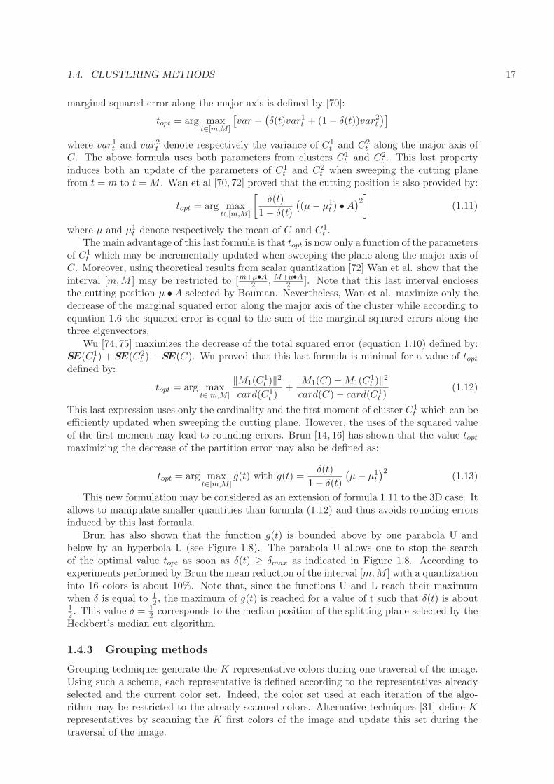
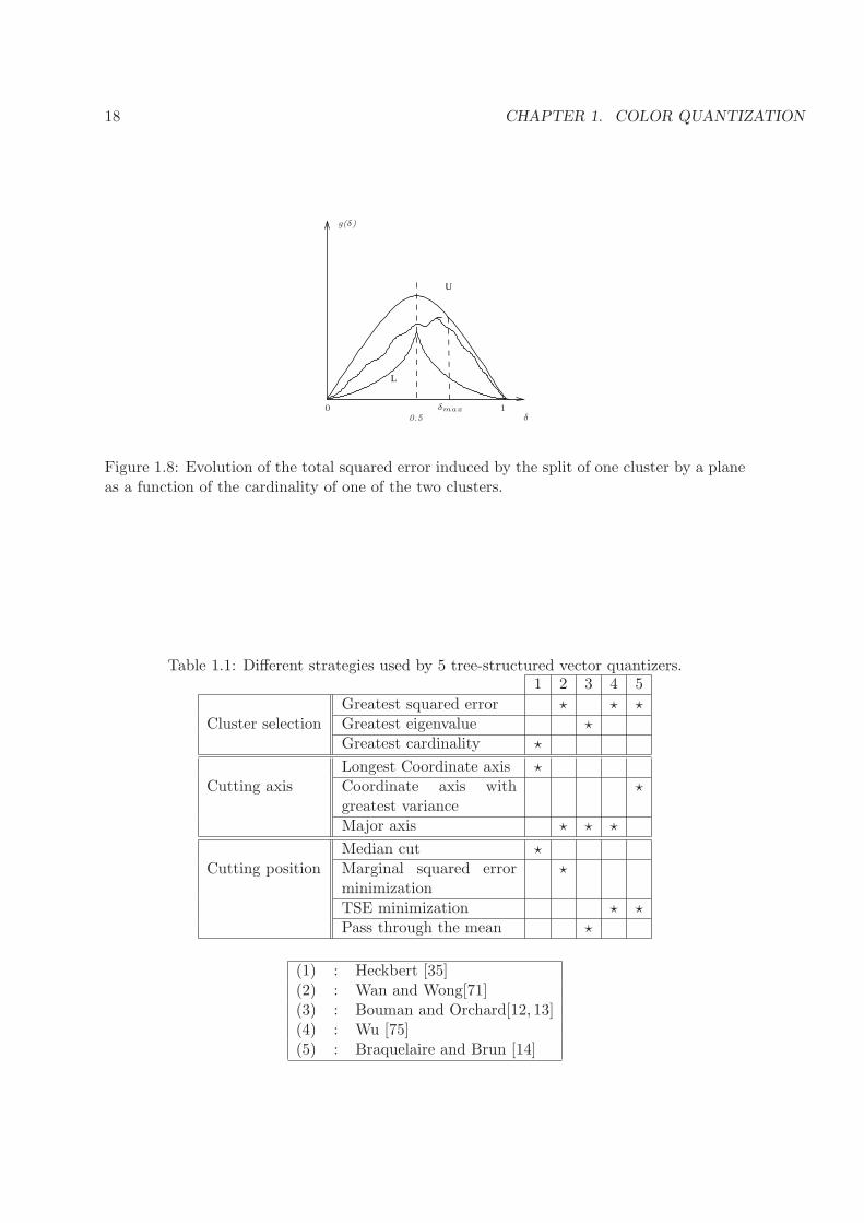
Brun has also shown that the function g(t) is bounded above by one parabola U andbelow by an hyperbola L (see Figure 1.8). The parabola U allows one to stop the searchof the optimal value topt as soon as δ(t) ≥ δmax as indicated in Figure 1.8. According toexperiments performed by Brun the mean reduction of the interval [m,M ] with a quantizationinto 16 colors is about 10%. Note that, since the functions U and L reach their maximumwhen δ is equal to 1
2 , the maximum of g(t) is reached for a value of t such that δ(t) is about12 . This value δ = 1
2 corresponds to the median position of the splitting plane selected by theHeckbert’s median cut algorithm.
1.4.3 Grouping methods
Grouping techniques generate the K representative colors during one traversal of the image.Using such a scheme, each representative is defined according to the representatives alreadyselected and the current color set. Indeed, the color set used at each iteration of the algo-rithm may be restricted to the already scanned colors. Alternative techniques [31] define Krepresentatives by scanning the K first colors of the image and update this set during thetraversal of the image.
18 CHAPTER 1. COLOR QUANTIZATION
L
U
g(δ)
0.5 δ0 1δmax
Figure 1.8: Evolution of the total squared error induced by the split of one cluster by a planeas a function of the cardinality of one of the two clusters.
Table 1.1: Different strategies used by 5 tree-structured vector quantizers.1 2 3 4 5
Greatest squared error ⋆ ⋆ ⋆Cluster selection Greatest eigenvalue ⋆
Greatest cardinality ⋆
Longest Coordinate axis ⋆Cutting axis Coordinate axis with
greatest variance⋆
Major axis ⋆ ⋆ ⋆
Median cut ⋆Cutting position Marginal squared error
minimization⋆
TSE minimization ⋆ ⋆Pass through the mean ⋆
(1) : Heckbert [35](2) : Wan and Wong[71](3) : Bouman and Orchard[12, 13](4) : Wu [75](5) : Braquelaire and Brun [14]
1.4. CLUSTERING METHODS 19
The merge and box algorithm.
This algorithm proposed by Fletcher [25] is based on an iterative process which is repeateduntil the boxes with the K representative colors are formed. This algorithm iterates thefollowing steps: each distinct color of the color space is placed into a sub-box of length sideequal to one. If the input color can be approximated, with an error no greater than half thelength of box’s diagonal, by one of the sub-boxes already generated this color is included inthe corresponding sub-box. Otherwise, a new sub-box of side one is added to the list. Toobtain a list which do not exceed K sub-boxes, a merging process is used when the numberof sub-boxes is equal to K + 1 to gather the pair of sub-boxes which must to be merged intoa single sub-box. The merging pair is the one which minimize the largest side of the mergedsub-box.
According to Fletcher [25], the heuristic used by the merger generates roughly cubicalsub-boxes with a similar size. Using a Manhattan distance between corners would result inelongated sub-boxes, causing larger quantization errors. This algorithm may be parallelizedon a SIMD parallel processor. Moreover, its calculating time may be further reduced by usinga spatial sampling to approximate accurately the image color set.
Gervautz [31] proposed a similar approach based on a hierarchical decomposition of theRGB cube by an octree. Using this decomposition each cube of side 1 used by Fetcher isencoded as a leaf of the octree. Gervautz builds the first K leaves of the octree by scanningthe first K colors of the image. Each leaf of the tree represents thus one cluster of the RGBcolor space. If an additional color belongs to one of these clusters, the mean color of theassociated leaf is updated and the structure of the octree remains unchanged. Otherwise, anew leaf is created from the merger of its children in order to keep only K leave. The set ofK representative colors is then defined from the centroid of the clusters associated to eachleaf of the octree.
The max-min algorithm.
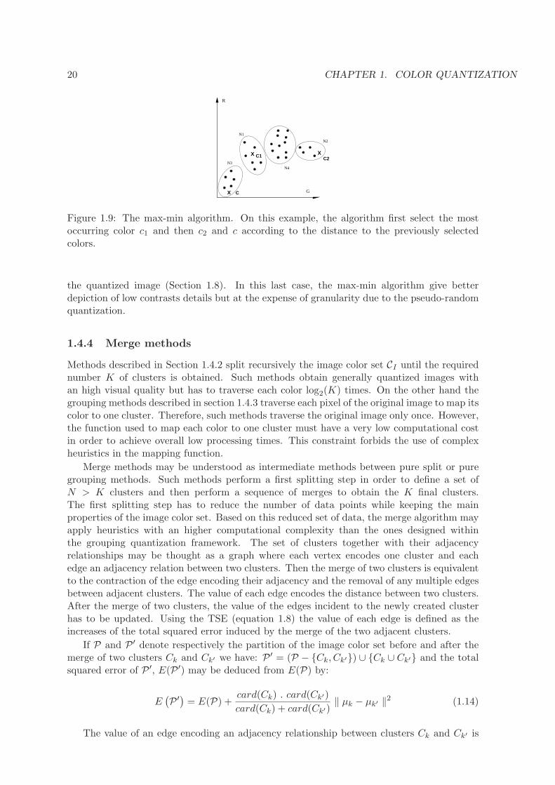
The max-min algorithm first proposed by Houle and Dubois[37] iterates the following steps(Figure 1.9):
1. a single color c1 is first selected from the original image. It could be the most frequentlyoccurring one.
2. A new representative color ck is then computed, ck is the un-selected color whose min-imum distance to any of the representative colors thus far selected is maximum, i.e., ckmust verify :
mink′=1,...k−1
‖ck − ck′‖2 ≥ min
k′=1,...k−1‖c− ck′‖
2 ∀c ∈ ΩI − ΩQ
where symbols ΩI and ΩQ denote respectively the image color set and the set of repre-sentatives already selected.
Step 2 of the max-min algorithm is iterated until K representative colors are selected.
A similar approach has been proposed by Xiang [76] who initializes the first color c1arbitrary. Note that, an arbitrary selection of the first color avoids the computation of theimage’s histogram. This quantization scheme has also been investigated by Tremeau et al.[64]to extend it to a vector quantization process based on the nearest color query principle.
According to Houle and Dubois the set of representatives generated by this algorithmis uniformly distributed and extends right to the boundary of the image color set. Thisdistribution is well suited when a pseudo-random noise vector is added to the color value ofthe pixel to be quantized, i.e., when we try to minimize errors of quantization by dithering
20 CHAPTER 1. COLOR QUANTIZATION
R
G
XX C1 C2
N1
N4
N2
N3
CX
Figure 1.9: The max-min algorithm. On this example, the algorithm first select the mostoccurring color c1 and then c2 and c according to the distance to the previously selectedcolors.
the quantized image (Section 1.8). In this last case, the max-min algorithm give betterdepiction of low contrasts details but at the expense of granularity due to the pseudo-randomquantization.
1.4.4 Merge methods
Methods described in Section 1.4.2 split recursively the image color set CI until the requirednumber K of clusters is obtained. Such methods obtain generally quantized images withan high visual quality but has to traverse each color log2(K) times. On the other hand thegrouping methods described in section 1.4.3 traverse each pixel of the original image to map itscolor to one cluster. Therefore, such methods traverse the original image only once. However,the function used to map each color to one cluster must have a very low computational costin order to achieve overall low processing times. This constraint forbids the use of complexheuristics in the mapping function.
Merge methods may be understood as intermediate methods between pure split or puregrouping methods. Such methods perform a first splitting step in order to define a set ofN > K clusters and then perform a sequence of merges to obtain the K final clusters.The first splitting step has to reduce the number of data points while keeping the mainproperties of the image color set. Based on this reduced set of data, the merge algorithm mayapply heuristics with an higher computational complexity than the ones designed withinthe grouping quantization framework. The set of clusters together with their adjacencyrelationships may be thought as a graph where each vertex encodes one cluster and eachedge an adjacency relation between two clusters. Then the merge of two clusters is equivalentto the contraction of the edge encoding their adjacency and the removal of any multiple edgesbetween adjacent clusters. The value of each edge encodes the distance between two clusters.After the merge of two clusters, the value of the edges incident to the newly created clusterhas to be updated. Using the TSE (equation 1.8) the value of each edge is defined as theincreases of the total squared error induced by the merge of the two adjacent clusters.
If P and P ′ denote respectively the partition of the image color set before and after themerge of two clusters Ck and Ck′ we have: P ′ = (P − Ck, Ck′) ∪ Ck ∪ Ck′ and the totalsquared error of P ′, E(P ′) may be deduced from E(P) by:
E(
P ′)
= E(P) +card(Ck) . card(Ck′)
card(Ck) + card(Ck′)‖ µk − µk′ ‖
2 (1.14)
The value of an edge encoding an adjacency relationship between clusters Ck and Ck′ is
1.4. CLUSTERING METHODS 21
thus equal to:
∆k,k′ =card(Ck) . card(Ck′)
card(Ck) + card(Ck′)‖ µk − µk′ ‖
2 (1.15)
Note that one is effectively minimizing a weighted Euclidean distance between the twocentroids µk and µk′ of the two clusters Ck and Ck′ . This is the reason why such methodsare often referenced as pairwise nearest neighbor clustering [10, 23].
The main computational cost of merge methods comes from the merger which has totraverse all pairs of adjacent clusters at each step. Two approaches have been proposed andsometimes combined [10] to reduce this computational cost: The reduction of the number ofinitial clusters and the use of heuristics in the merge strategy.
Brun and Mokhtari [17] first perform a uniform quantization of the RGB cube into Nclusters and then create a complete graph from the set of clusters. This graph is reducedby merging at each step the two closest clusters according to equation 1.14. Experimentsperformed by Brun et al. show that if K is lower than 16, very low values of N such as 200or 300 are sufficient to obtain high quality quantized images.
Dixit [22] reduces the initial number of clusters by a sub sampling of the image at randomlocations. According to Dixit, as few as 1024 random locations on a 512 × 512 image aresufficient to obtain a good estimate of the distribution of the image color set. The set ofclusters is then sorted in ascending order according to the cardinality of each cluster. Thesorted table of clusters is then traversed from the clusters with lowest cardinality and eachcurrent cluster is paired with the closest remaining one according to equation 1.14. These twoclusters are then excluded from the merge. Therefore, no cluster is allowed to be paired withmore than one cluster and the set of clusters is reduced by a factor two at each iteration. Notethat this fixed decimation ratio between two successive iterations may lead to the merger ofclusters which are far apart.
Xiang and Joy [77] create the initial set of clusters by using a uniform quantization ofthe RGB color space into N clusters. Xiang reduces the N initial clusters to K final clustersby a sequence of N −K merges. At each step, the merge criterion selects two clusters suchthat the newly created cluster is enclosed into a minimal bounding box. Xiang thus estimatesthe homogeneity of one cluster by the size of its bounding box. Using an initial uniformquantization into 2× 1× 4 boxes, each cluster has approximately the same luminance in theY IQ-NTSC system. Therefore, the size of a bounding box may be understood as the shiftin luminance within the associated cluster and Xiang algorithm mainly attempts to minimizethe shift in luminance within the quantized image. Such shifts may produce significant visualartifacts in the ray-traced images used by Xiang.
Equitz [23] reduces the computational cost of the merger by using a k − d tree (seeSection 1.7.3) which decomposes the set of initial clusters into a set of regions each composedof 8 clusters. The complete graph defined by Brun [17] is thus decomposed into a set ofnon-connected complete sub-graphs, each composed of 8 vertices. Then, Equitz finds the twoclosest clusters in each sub-graph according to equation 1.14 and merges a fixed fraction ofthem (such as 50%). After each iteration, the decomposition of the initial graph into regions isalso updated in order to obtain roughly equal size sub-graphs. Note that this merge strategyneglects adjacencies between vertices belonging to different sub-graphs. Equitz’s heuristic hasbeen improved by Balasubramanian and Allebach [10] who first perform a prequantizationstep described in Section 1.5. Balasubramanian also weights the distance between two clustersby an activity measure defined from the initial image (Section 1.5).
1.4.5 Popularity methods
This family of methods, introduced by Heckbert [35], uses the histogram of the image color setto define the set of representatives as the K most occurring colors in the image. This simple
22 CHAPTER 1. COLOR QUANTIZATION
and efficient algorithm may however perform poorly on images with a wide range of colors.Moreover it often neglects color in sparse regions of the color set. Likewise, this algorithmperforms poorly when asked to quantize to a small number of colors (say < 50) [35].
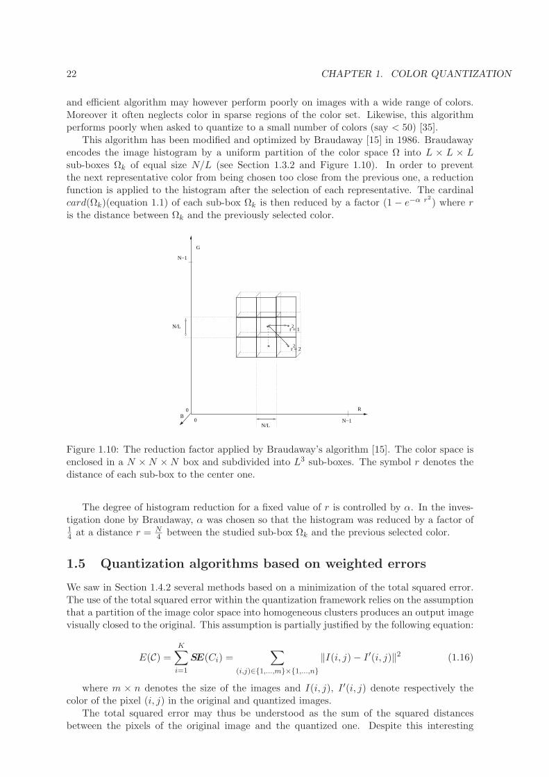
This algorithm has been modified and optimized by Braudaway [15] in 1986. Braudawayencodes the image histogram by a uniform partition of the color space Ω into L × L × Lsub-boxes Ωk of equal size N/L (see Section 1.3.2 and Figure 1.10). In order to preventthe next representative color from being chosen too close from the previous one, a reductionfunction is applied to the histogram after the selection of each representative. The cardinalcard(Ωk)(equation 1.1) of each sub-box Ωk is then reduced by a factor (1 − e−α r2) where ris the distance between Ωk and the previously selected color.
* *
* r = 22
r = 12
*
0N/L
G
BR
N−1
0
N−1
N/L
Figure 1.10: The reduction factor applied by Braudaway’s algorithm [15]. The color space isenclosed in a N ×N ×N box and subdivided into L3 sub-boxes. The symbol r denotes thedistance of each sub-box to the center one.
The degree of histogram reduction for a fixed value of r is controlled by α. In the inves-tigation done by Braudaway, α was chosen so that the histogram was reduced by a factor of14 at a distance r = N
4 between the studied sub-box Ωk and the previous selected color.
1.5 Quantization algorithms based on weighted errors
We saw in Section 1.4.2 several methods based on a minimization of the total squared error.The use of the total squared error within the quantization framework relies on the assumptionthat a partition of the image color space into homogeneous clusters produces an output imagevisually closed to the original. This assumption is partially justified by the following equation:
E(C) =K∑
i=1
SE(Ci) =∑
(i,j)∈1,...,m×1,...,n
‖I(i, j)− I ′(i, j)‖2 (1.16)
where m × n denotes the size of the images and I(i, j), I ′(i, j) denote respectively thecolor of the pixel (i, j) in the original and quantized images.
The total squared error may thus be understood as the sum of the squared distancesbetween the pixels of the original image and the quantized one. Despite this interesting
1.5. QUANTIZATION ALGORITHMS BASED ON WEIGHTED ERRORS 23
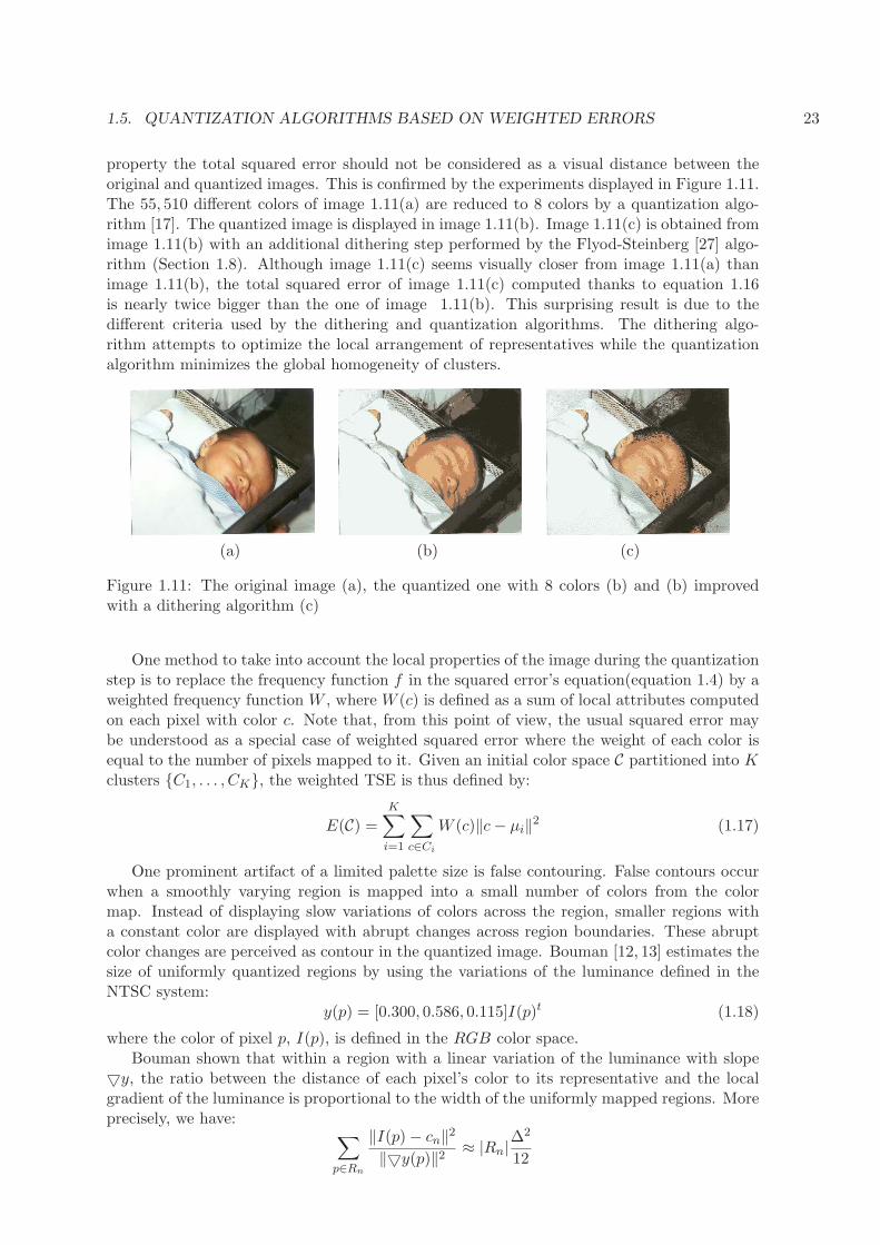
property the total squared error should not be considered as a visual distance between theoriginal and quantized images. This is confirmed by the experiments displayed in Figure 1.11.The 55, 510 different colors of image 1.11(a) are reduced to 8 colors by a quantization algo-rithm [17]. The quantized image is displayed in image 1.11(b). Image 1.11(c) is obtained fromimage 1.11(b) with an additional dithering step performed by the Flyod-Steinberg [27] algo-rithm (Section 1.8). Although image 1.11(c) seems visually closer from image 1.11(a) thanimage 1.11(b), the total squared error of image 1.11(c) computed thanks to equation 1.16is nearly twice bigger than the one of image 1.11(b). This surprising result is due to thedifferent criteria used by the dithering and quantization algorithms. The dithering algo-rithm attempts to optimize the local arrangement of representatives while the quantizationalgorithm minimizes the global homogeneity of clusters.
(a) (b) (c)
Figure 1.11: The original image (a), the quantized one with 8 colors (b) and (b) improvedwith a dithering algorithm (c)
One method to take into account the local properties of the image during the quantizationstep is to replace the frequency function f in the squared error’s equation(equation 1.4) by aweighted frequency function W , where W (c) is defined as a sum of local attributes computedon each pixel with color c. Note that, from this point of view, the usual squared error maybe understood as a special case of weighted squared error where the weight of each color isequal to the number of pixels mapped to it. Given an initial color space C partitioned into Kclusters C1, . . . , CK, the weighted TSE is thus defined by:
E(C) =K∑
i=1
∑
c∈Ci
W (c)‖c− µi‖2 (1.17)
One prominent artifact of a limited palette size is false contouring. False contours occurwhen a smoothly varying region is mapped into a small number of colors from the colormap. Instead of displaying slow variations of colors across the region, smaller regions witha constant color are displayed with abrupt changes across region boundaries. These abruptcolor changes are perceived as contour in the quantized image. Bouman [12, 13] estimates thesize of uniformly quantized regions by using the variations of the luminance defined in theNTSC system:
y(p) = [0.300, 0.586, 0.115]I(p)t (1.18)
where the color of pixel p, I(p), is defined in the RGB color space.Bouman shown that within a region with a linear variation of the luminance with slope
y, the ratio between the distance of each pixel’s color to its representative and the localgradient of the luminance is proportional to the width of the uniformly mapped regions. Moreprecisely, we have:
∑
p∈Rn
‖I(p)− cn‖2
‖y(p)‖2≈ |Rn|
∆2
12
24 CHAPTER 1. COLOR QUANTIZATION
where Rn denotes the set of pixels p whose color I(p) is mapped to cn. The cardinality of thisset is denoted by |Rn|. The symbol ∆ denotes the width of an uniformly quantized regionsin the direction of the luminance gradient y.
Therefore, in order to minimize the size of the uniformly mapped regions (estimated by∆), Bouman uses a weighting inversely proportional to the luminance gradient of the image.For each color c of the original image, the weighting W (c) is defined by:
W (c) =∑
p∈I|I(p)=c
(
1
h ⋆min‖y(p)‖, 16+ 2
)2
(1.19)
where the constants 16 and 2 bound the dynamic range of the gradient, while the function his a smoothing kernel the convolution of which allows to estimate the mean gradient over theregions.
Note that any scale of the luminance component in the original image by a factor s scalesthe weighting factor W (sc) by 1
s2while the squared distance between c and its representative
is scaled by a factor s2. Therefore, the factors W (c)‖c − ci‖2 and the weighted TSE (see
equation 1.17) are insensitive to any global scaling of the luminance. This obeys Weber’slaw [55], which suggests that any measure of subjective image quality should be invariant toabsolute intensity scaling.
Bouman integrates the weighting defined by equation 1.19 into a tree structured vectorquantizer (Section 1.4.2 and Table 1.1). Using the weighted TSE (equation 1.17), the weightedmoments of a cluster C are simply defined by substituting f(c) by W (c) in equations 1.1.The weighted mean and covariance of the cluster are then defined from the weighted momentsusing equation 1.2. Bouman uses the weighted mean µw
i and covariance matrix Covwi of eachcluster Ci to adapt his tree-structured vector quantizer as follows:
1. Select the cluster Cm whose weighted covariance matrix has the greatest eigenvalue.Let us denote by em the eigenvector associated with this eigenvalue.
2. Split the selected cluster by a plane orthogonal to em and passing through µwm.
Note that since the introduction of weights modifies the distribution of the initial imagecolor set, it modifies all key steps of Bouman’s recursive split algorithm. Moreover, theweights introduced by Bouman may be easily adapted to other recursive splitting schemes.For example, a weighted minimization of the TSE may be achieved by computing the weightedsquared error using the weighted moments (see equations 1.19 and 1.7) and selecting at eachstep the cluster whose weighted squared error is maximal.
One other characteristic of the Human Visual System is its greater sensitivity to quan-tization errors in smooth areas than in busy regions of the image. Balasubramanian andAllebach [8, 10] define a color activity measure on each pixel by:
αk =1
64
∑
p∈Pk
‖cp − ck‖
where Pk is a 8× 8 block centered around pixel k. The symbols cp and ck denote respectivelythe color of pixel p and the mean color of Pk.
These values are then accumulated on colors by associating to each color the minimalcolor activity measure of the color over all spatial blocks:
αc = mink∈Kc
αk (1.20)
where Kc denotes the set of blocks in which color c occurs.
1.5. QUANTIZATION ALGORITHMS BASED ON WEIGHTED ERRORS 25
Since luminance component has the greatest variations, the gradient of the luminanceis also used as an alternative [9] or to complement [10] the measure of the spatial masking.Experiments show that the masking of quantization noise by image activity at a pixel dependsnot only on the luminance gradient at the pixel but also on gradients at the neighboringpixels. Based on these experiments, Ballasubramanian [9, 10] computes the gradient y ofthe luminance defined in the NTSC system (equation 1.18) on each pixel. Then, the luminanceactivity αl
k of each 8× 8 block k is defined as an average value of its gradient. The luminanceactivity of each color is then defined as the average value of the block’s gradient in which thiscolor occurs:
αlc =
1
|Kc|
∑
k∈Kc
αlk (1.21)
where Kc denotes the set of blocks in which color c occurs.
The color or luminance activity may then be used to weight the colors during the quanti-zation step. Balasubramanian chose W (c) = 1
αcand W (c) = 1
αc2 respectively in [9] and [10].
In both cases, the importance of colors with low activity measure is reinforced by the weight-ing to the detriment of colors with high activity measure whose quantization errors are lessreadily perceived by the human visual system.
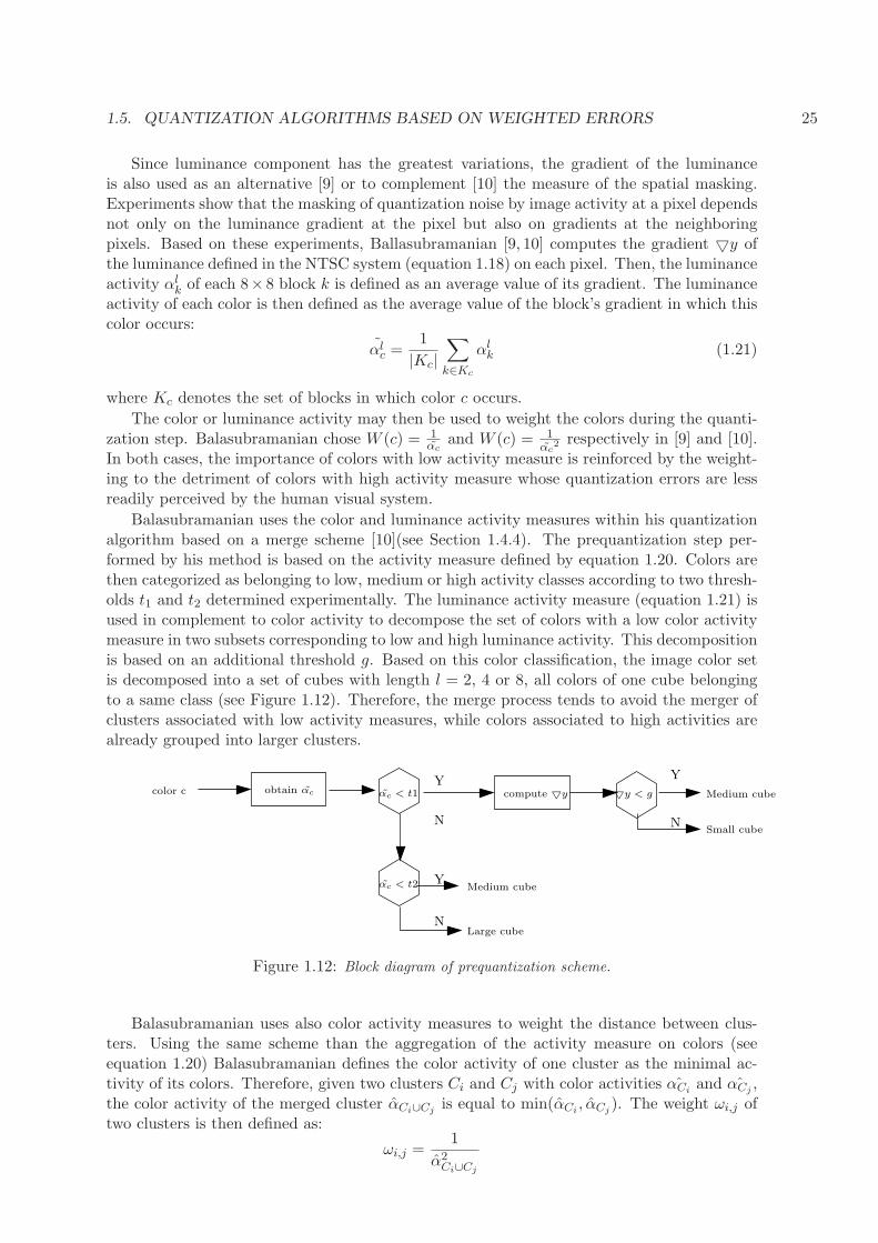
Balasubramanian uses the color and luminance activity measures within his quantizationalgorithm based on a merge scheme [10](see Section 1.4.4). The prequantization step per-formed by his method is based on the activity measure defined by equation 1.20. Colors arethen categorized as belonging to low, medium or high activity classes according to two thresh-olds t1 and t2 determined experimentally. The luminance activity measure (equation 1.21) isused in complement to color activity to decompose the set of colors with a low color activitymeasure in two subsets corresponding to low and high luminance activity. This decompositionis based on an additional threshold g. Based on this color classification, the image color setis decomposed into a set of cubes with length l = 2, 4 or 8, all colors of one cube belongingto a same class (see Figure 1.12). Therefore, the merge process tends to avoid the merger ofclusters associated with low activity measures, while colors associated to high activities arealready grouped into larger clusters.
color c obtain αc
Y
N
compute y
Medium cube
Medium cube
Small cube
Large cube
y < g
Y
N
Y
N
αc < t1
αc < t2
Figure 1.12: Block diagram of prequantization scheme.
Balasubramanian uses also color activity measures to weight the distance between clus-ters. Using the same scheme than the aggregation of the activity measure on colors (seeequation 1.20) Balasubramanian defines the color activity of one cluster as the minimal ac-tivity of its colors. Therefore, given two clusters Ci and Cj with color activities αCi
and ˆαCj,
the color activity of the merged cluster αCi∪Cjis equal to min(αCi
, αCj). The weight ωi,j of
two clusters is then defined as:
ωi,j =1
α2Ci∪Cj
26 CHAPTER 1. COLOR QUANTIZATION
In order to attach large weights to distance between clusters with small activities and viceversa Balasubramanian defines the weighted distance between clusters Ci and Cj as ωi,j∆i,j
where ∆i,j is the increase of the total squared error induced by the merge of clusters Ci andCj (equation 1.14). Using such weights, clusters with high activity measure are more likelyto be merged before low activity clusters.
Balasubramanian and Bouman combined their methods [8] in order to integrate the colorweights defined by Balasubramanian within the tree-structured vector quantizer defined byBouman. This method defines the aggregate weight of each cluster as the average weightof its colors. Since the cluster’s weights are more meaningful for small and close clusters,Balasubramanian et al. perform 2
3K un-weighted binary split (Section 1.4.2 and Table 1.1).Then the 1
3K remaining splits are performed by splitting at each step the cluster whoseweighted eigenvalue ωkλk is maximal. The symbols ωk and λk denote respectively the weightand the maximal eigenvalue of cluster Ck.
1.6 Post clustering methods
Quantization strategies presented so far use a pre-clustering scheme which computes the set ofrepresentatives only once. Another strategy consists to define an initial set of representativesand to improve it iteratively. Such a quantization scheme is called a post-clustering strategy.While the pre-clustering strategy is commonly used, the post-clustering one is less popular.Indeed, the use of a post-clustering strategy induces generally three main drawbacks: First,the number of iterations being not bounded, quantization algorithms using a post-clusteringscheme may be computationally intensive. A much bigger disadvantage generally is the lossof the structure induced by the original strategy, which often makes the mapping step verycomputation intensive. Lastly, the iterative improvement of the set of representatives gen-erally converges to the local minimum the closest from the initial solution. Therefore, suchalgorithms are often trapped into local minima of the optimized criterion. However, severalheuristics, presented in this section have been proposed to improve the computational effi-ciency of post-clustering algorithms. Moreover, using a post-clustering scheme, informationssuch as the interrelationships between neighboring clusters or the spatial distribution of col-ors may be naturally integrated into quantization algorithms. Finally, one common heuristicconsists to combine the pre and post-quantization schemes as follows: First, an initial setof representatives closed from the optimal solution is determined by a pre-quantization algo-rithm. This initial set of representative is then moved to the (hopefully) global optimum bya quantization algorithm based on a post-clustering scheme.
1.6.1 The LBG and k-means algorithms
Let us first introduce the LBG algorithm. The design of a locally optimal vector quantizers wasboth investigated by Llyod in 1982 [47], and by Linde et al. in 1980 [46]. The initializationstep defines one set of representatives. This could be the K most occurring colors or anyset of colors chosen arbitrary. The iteration begins by assigning each input color to onerepresentative according to some distortion measure. These assignments define a partition ofthe image color set into clusters, each cluster being associated to one representative. The setof representatives is then modified to minimize the errors relative to input colors. This twostep process is iterated until no significant change occurs within the set of representativesbetween two successives iterations.
Several quantization processes, such as those proposed by Heckbert [35] or Braudaway [15],use the LBG algorithm to improve the set of representatives obtained from their quantizers.However, since the LBG algorithm converges only to a local minimum, this step often yields
1.6. POST CLUSTERING METHODS 27
only slight improvements [58].
Several investigations have been performed to improve the performance of this algorithm,such as the one by Goldberg [32], who extends this algorithm to a high resolution solutionwhich selects a set of representative vectors from input vectors. Likewise, Feng [24] hasextended this algorithm to a vector quantizer that exploits the statistical redundancy betweenthe neighboring blocks to reduce the bit rate required by the algorithm.
More significant improvements can be obtained thanks to other heuristics that attempt toselect the palette through a sequential splitting process while reducing the TSE at each step.Several investigations such that those of Orchard and Bouman [13] or the one of Balasubra-manian [8] propose various splitting procedures and different selection criteria to reduce theTSE.
The k-means algorithms belong to the same category of post-clustering techniques. Thesealgorithms are based on an iterative process which is repeated until it converges to a localminimum solution, e.g. until the cluster centers of the K generated clusters do not changefrom one iteration to the other. The number of iterations required by the algorithm dependson the distribution of the color points, the number of requested clusters, the size of the colorspace and the choice of initial cluster centers [70]. Consequently, for a large clustering problem,the computation can be very time consuming. Recently, faster clustering approaches havebeen proposed. Among them, some are commonly used in color image quantization [56], evenif these approaches have been originally developed to color image segmentation applicationssuch as the C-means [19], the fuzzy C-means [43] and the genetic C-means [56] clusteringalgorithms or the hierarchical merging approach [7].
1.6.2 The NeuQuant Neural-Net image quantization algorithm
The NeuQuant Neural-Net image quantization algorithm has been developed to improvethe common Median Cut algorithm (Section 1.4.2). This algorithm operates using a one-dimensional self-organizing Kohonen Neural Network, typically with 256 neurons, which self-organizes through learning to match the distribution of colors in an input image. Taking theposition in RGB-space of each neuron gives a high-quality color map in which adjacent colorsare similar.
By adjusting a sampling factor, the network can either produce extremely high-qualityimages slowly, or produce good images in reasonable times. With a sampling factor of 1, theentire image is used in the learning phase, while with a factor of e.g. 10, a pseudo-randomsubset of 1/10 of the pixels are used in the learning phase. A sampling factor of 10 givesa substantial speed-up, with a small quality penalty. Careful coding and a novel indexingscheme are used to make the algorithm efficient. This confounds the frequent observationthat Kohonen Neural Networks are necessarily slow.
1.6.3 The local k-means algorithm.
The local K-means algorithm (LKM), which has been introduced by Verevka and Buchanan[68, 69] is an iterative post-clustering technique that approximates an optimal palette usingmultiple subsets of image points. This method is based on a combination of a K-meansquantization process and a self-organizing map (or Kohonen neural network). The aim of thismethod is to minimize simultaneously both the TSE and the standard deviation of squarederror of pixels σ =
√∑
c∈C(‖c− q(c)‖ − E(C))2/card(C). Meanwhile small values of theTSE guarantee that a quantization process accurately represents colors of the original image,the minimization of the standard deviation preserves variations of colors in the quantizedimage. The main limitation of this method comes from the two measures used which treateach pixel independently. Consequently the spatial correlation among colors is not taken into
28 CHAPTER 1. COLOR QUANTIZATION
account. The main advantage of this method is its ability to select a palette without makingany assumptions about the boundaries of color clusters.
1.7 Mapping methods
The inverse colormap operation is the process which maps an image into a limited set ofrepresentative colors. These representatives may be defined by a quantization algorithmor imposed by the default colormap of the output device. In order to minimize the visualdistortion between the input image and the output one, inverse colormap algorithms mapeach color c of the input image to its nearest representative Q(c). The function Q may bedefined by :
C → c1, . . . , cKc 7→ Q(c) = argminz∈c1,...,cK ‖z − c‖
(1.22)
where C represents the set of colors of the input image, and c1, . . . , cK the set of rep-resentative colors. The symbol ‖z − c‖ denotes the Euclidean norm of the 3D vector z − ccomputed in a given color space.
The value Q(c) for a given color c may be computed thanks to an exhaustive search ofthe minimum of ‖z− c‖ for all representative colors. Given a 256×256 image and a colormapof 256 colors, this trivial algorithm requires more than sixteen million distance computations(see equation 1.22). Thus, despite its simplicity and the fact that this method provides anexact solution, it is not practical for large images or interactive applications. Several methodsdescribed below have thus been designed to optimize the search of the closest representative.The complexity of the main algorithms is resumed in Table 1.2.
1.7.1 Improvements of the trivial inverse colormap method
The improvements of the trivial inverse colormap algorithm are numerous: Poskanzer [52]proposed improving the search by using a hash table which allows one to avoid the searchof the nearest representative for any color already encountered. However, this optimizationremains inefficient for images with a large set of different colors such as outdoor scenes. Oneother approach consists to approximate the L2 Euclidean norm by a less expensive distancemetric. Chaudhuri et al. [20] proposed the Lα norm as an approximation of the Euclideandistance. The Lα norm of a color c being defined by:
‖c‖α = (1− α)‖c‖1 + α‖c‖∞= (1− α)
∑3j=1 |c
j |+ αmaxi∈1,2,3 |cj |
According to experiments performed by Verevka [68] the L 1
2
norm speeds up significantly the
search without introducing a noticeably loss in output image quality.The search can be further reduced by using the following considerations [36]:
• Partial sum: Using the square of the L2 distance, the L1 norm or the L 1
2
norm the
distance between the input color and one representative is defined as a sum of threeterms. The partial sum should be compared to the current minimal distance beforeeach new addition. The distance calculation terminates is the partial sum is greaterthan the current minimal distance.
• Sorting on one coordinate: Let us assume that the representatives are sorted along onecoordinate axis (e.g. the first one). Then the search starts with the representative whosefirst coordinate is the closest from the input color and continue in the increasing firstcoordinate distance order. The process terminates when the first coordinate distance
1.7. MAPPING METHODS 29
between the next representative and the input color is greater than the current minimaldistance. Note that one should use an axis with a large variance to accelerate thetermination of the search.
• Nearest neighbor distance: Given a representative cj with j ∈ 1, . . . ,K its closestrepresentative cq(j) is defined by:
q(j) = arg mink∈1,...,K,k 6=j
d(cj , ck)
Let us suppose that the current representative ci traversed by the inverse colormapalgorithm is the current closest representative from the input color c. We additionallysuppose that the current minimal distance Σmin = d(c, ci) is less than one half ofd(ci, cq(i)). We have thus:
Σmin = d(c, ci)Σmin ≤ 1
2d(ci, cq(i))
Then, given any other representative color ck:
2Σmin ≤ d(ci, cq(i)) ≤ d(ci, ck) ≤ d(ci, c) + d(c, ck)
⇒ 2Σmin ≤ Σmin + d(c, ck)⇒ Σmin ≤ d(c, ck)
The inverse colormap algorithm should then terminate since no representative may beclosest from c than ci.
1.7.2 Inverse colormap algorithms devoted to a specific quantization method
As mentioned in Section 1.1 (see also Figure 1.1) any quantization algorithm requires aninverse colormap step. The set of representatives defined by quantization algorithms is builtin order to minimize a quantization error defined within some color space (e.g. CIELuvor Y IQ). On the other hand, inverse colormap algorithms map each color to its nearestrepresentative using an Euclidean norm also defined within a given color space. Therefore, theinverse colormap algorithm should use the same color space than the quantization algorithmin order to be consistent with the criterion used to design the set of representatives.
The assignment of each color to its nearest representative by inverse colormap algorithmsinduces a partition of the image color set by a three-dimensional Voronoı diagram defined bythe representatives. The partition defined by pre-clustering quantization methods generallydoes not constitute a Voronoı diagram but may be used as a close approximation of it if thepartition has a low total squared error. Moreover, using the partition defined by quantiza-tion algorithms, data structures generated by these algorithms may be used to reduce thecomputation cost of the mapping function. For example, using a tree-structured vector quan-tizer (Section 1.4.2), the binary tree generated by the quantization algorithm may be used toretrieve the representative of an input color with approximately O(log2(K)) operations.
1.7.3 Inverse colormap operations using k − d trees
Inverse colormap methods may also be studded within the more general nearest neighborframework. Friedman [11] proposed an algorithm based on an optimized k−d tree to determinethe m nearest neighbors of a given color. Given a set of colors, the k − d tree is built by arecursive bipartitioning scheme (Section 1.4.2), each cluster being split along its coordinateaxis with the greatest variance in order to have an equal number of colors in both sub clusters.
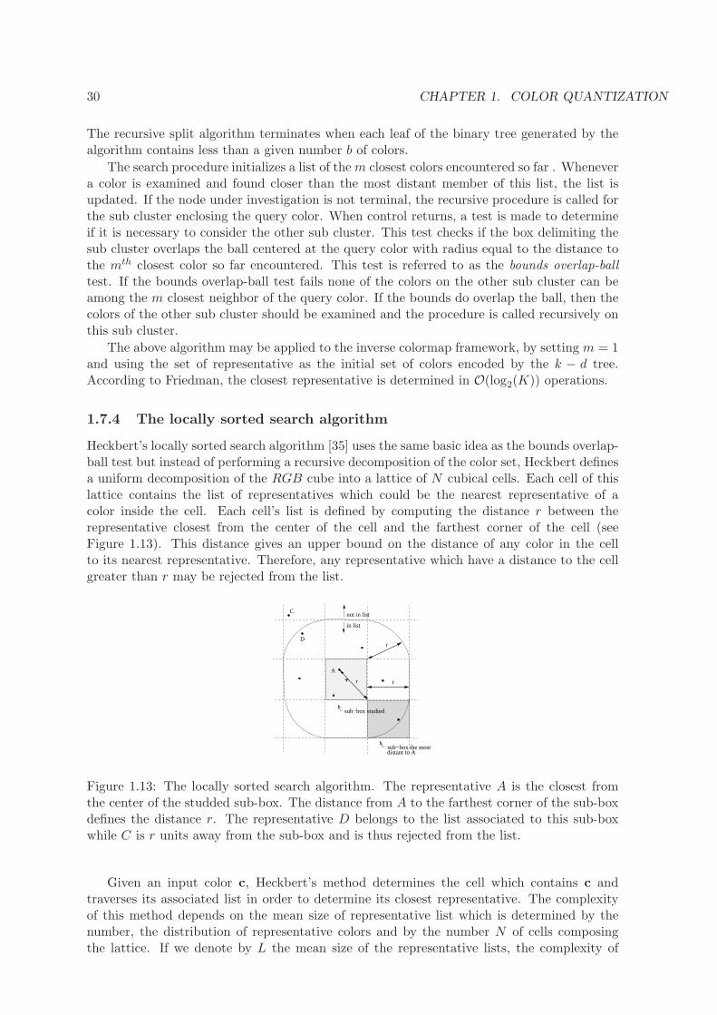
30 CHAPTER 1. COLOR QUANTIZATION
The recursive split algorithm terminates when each leaf of the binary tree generated by thealgorithm contains less than a given number b of colors.
The search procedure initializes a list of them closest colors encountered so far . Whenevera color is examined and found closer than the most distant member of this list, the list isupdated. If the node under investigation is not terminal, the recursive procedure is called forthe sub cluster enclosing the query color. When control returns, a test is made to determineif it is necessary to consider the other sub cluster. This test checks if the box delimiting thesub cluster overlaps the ball centered at the query color with radius equal to the distance tothe mth closest color so far encountered. This test is referred to as the bounds overlap-balltest. If the bounds overlap-ball test fails none of the colors on the other sub cluster can beamong the m closest neighbor of the query color. If the bounds do overlap the ball, then thecolors of the other sub cluster should be examined and the procedure is called recursively onthis sub cluster.
The above algorithm may be applied to the inverse colormap framework, by setting m = 1and using the set of representative as the initial set of colors encoded by the k − d tree.According to Friedman, the closest representative is determined in O(log2(K)) operations.
1.7.4 The locally sorted search algorithm
Heckbert’s locally sorted search algorithm [35] uses the same basic idea as the bounds overlap-ball test but instead of performing a recursive decomposition of the color set, Heckbert definesa uniform decomposition of the RGB cube into a lattice of N cubical cells. Each cell of thislattice contains the list of representatives which could be the nearest representative of acolor inside the cell. Each cell’s list is defined by computing the distance r between therepresentative closest from the center of the cell and the farthest corner of the cell (seeFigure 1.13). This distance gives an upper bound on the distance of any color in the cellto its nearest representative. Therefore, any representative which have a distance to the cellgreater than r may be rejected from the list.
+
sub−box studied
in list
not in listC
D
A
r r
r
sub−box the mostdistant to A
Figure 1.13: The locally sorted search algorithm. The representative A is the closest fromthe center of the studded sub-box. The distance from A to the farthest corner of the sub-boxdefines the distance r. The representative D belongs to the list associated to this sub-boxwhile C is r units away from the sub-box and is thus rejected from the list.
Given an input color c, Heckbert’s method determines the cell which contains c andtraverses its associated list in order to determine its closest representative. The complexityof this method depends on the mean size of representative list which is determined by thenumber, the distribution of representative colors and by the number N of cells composingthe lattice. If we denote by L the mean size of the representative lists, the complexity of
1.7. MAPPING METHODS 31
the preprocessing step which defines the lattice of N cells and sort the representative listsis equal to O(NK +NL log(L)) [35]. Experiments performed by Heckbert show that thenumber of distance computations required to determine the representative Q(c) of a color cmay be decreased by 23 for 256 representative colors and 512 cells. Nevertheless, with a fixednumber N of cells, this method remains approximately linear with respect to the number Kof representatives. Moreover, the optimal number N of cells is difficult to estimate.
Locally sorted search shows the greatest advantage over exhaustive search when K islarge and when the colors in the input image have a wide distribution [35]. In these cases thepre-processing time to create the database is overshadowed by the savings in search time.
Some variants of this algorithm such as those of Houle and Dubois [37] or Goldberg [32]have been proposed.
1.7.5 Inverse colormap operation using a 3D Voronoı diagram
Thomas’s method [60] computes the values of the function Q thanks to a 3D discrete Voronoıdiagram defined by the representative colors of the colormap. A discrete Voronoı diagramdefined by p points is a partition of a discrete image into a set of p cells, all pixels of onecell being closer from one representative than the others. One advantage of discrete Voronoıdiagrams beside real ones is that they can be computed thanks to incremental methods whichinitialize the n-dimensional image to be partitioned. Thus, using a discrete Voronoı diagram,the cell enclosing a given pixel is retrieved by reading its index in the n-dimensional image.
Using Thomas method, the Voronoı diagram is encoded thanks to a 3D array of integers.Each entry of this array represents a color and contains the index of its nearest representative.The main advantage of Thomas’s method is that once the 3D array encoding the 3D Voronoıdiagram has been computed the representative of any input color may be retrieved without anycomputation. This method is thus quite adapted to map any color to the default colormap of ascreen. However, it has several drawbacks: First, this algorithm computes the representativeof each displayable color. Thus, it involves many useless computations when applied to a fewimages. Secondly, using the RGB color space, the computation of the 3D Voronoı diagramrequires the storage of 2563 indexes. In order to reduce the number of initialized values andthe amount of required memory, Thomas removes the three least significant bits of each R,G and B component. The 3D Voronoi diagram is then computed on a 32 × 32 × 32 cube.This heuristic decreases significantly the amount of required memory but introduces severalquantization errors (Section 1.2). Moreover, many quantization methods [14, 70, 74] use colorspaces such as CIELuv, CIELab [59] or Y CrCb [10] which are more adapted to human visionthan the RGB one. In this case, the inverse colormap algorithm has to use the same colorspace (Section 1.7.2). Using Thomas’s method and a different color space than the RGB one,we have to allocate and initialize a 3D image which encloses the transformation of the RGBspace. This constraint reinforces the problems linked to the number of data which must beallocated and initialized.
1.7.6 Inverse colormap operation by a 2D Voronoı diagram
The basic idea of this method proposed by Brun [18] approximates the 3D image color setby one of its 2D projection in order to perform the inverse colormap operation with a 2DVoronoı diagram instead of a 3D one. Experiments performed by Ohta [48] show that up to99% of the information (see equation1.3, Section 1.4) of an image color set is contained in theplane defined by the first two eigenvectors of the covariance matrix.
Given an image color set, Brun computes the first two eigenvectors of the covariancematrix (equation 1.2) and defines a projection operator p onto the plane Pprinc defined by
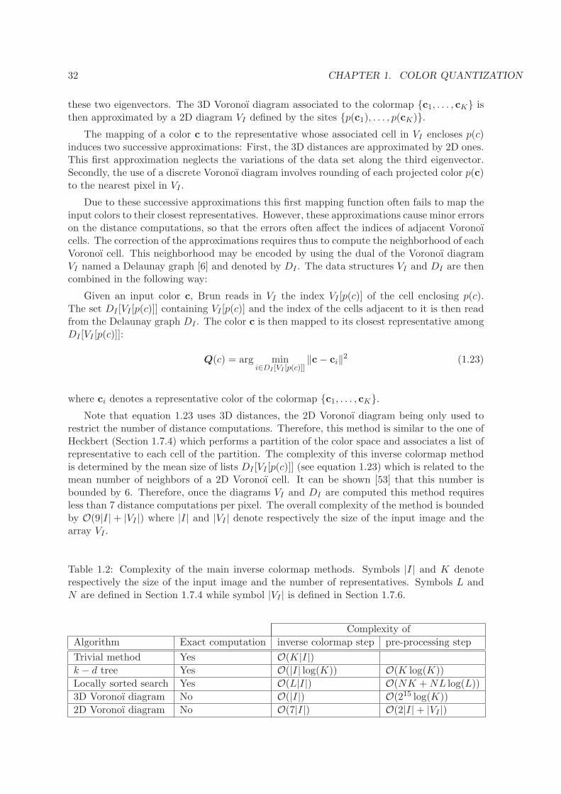
32 CHAPTER 1. COLOR QUANTIZATION
these two eigenvectors. The 3D Voronoı diagram associated to the colormap c1, . . . , cK isthen approximated by a 2D diagram VI defined by the sites p(c1), . . . , p(cK).
The mapping of a color c to the representative whose associated cell in VI encloses p(c)induces two successive approximations: First, the 3D distances are approximated by 2D ones.This first approximation neglects the variations of the data set along the third eigenvector.Secondly, the use of a discrete Voronoı diagram involves rounding of each projected color p(c)to the nearest pixel in VI .
Due to these successive approximations this first mapping function often fails to map theinput colors to their closest representatives. However, these approximations cause minor errorson the distance computations, so that the errors often affect the indices of adjacent Voronoıcells. The correction of the approximations requires thus to compute the neighborhood of eachVoronoı cell. This neighborhood may be encoded by using the dual of the Voronoı diagramVI named a Delaunay graph [6] and denoted by DI . The data structures VI and DI are thencombined in the following way:
Given an input color c, Brun reads in VI the index VI [p(c)] of the cell enclosing p(c).The set DI [VI [p(c)]] containing VI [p(c)] and the index of the cells adjacent to it is then readfrom the Delaunay graph DI . The color c is then mapped to its closest representative amongDI [VI [p(c)]]:
Q(c) = arg mini∈DI [VI [p(c)]]
‖c− ci‖2 (1.23)
where ci denotes a representative color of the colormap c1, . . . , cK.
Note that equation 1.23 uses 3D distances, the 2D Voronoı diagram being only used torestrict the number of distance computations. Therefore, this method is similar to the one ofHeckbert (Section 1.7.4) which performs a partition of the color space and associates a list ofrepresentative to each cell of the partition. The complexity of this inverse colormap methodis determined by the mean size of lists DI [VI [p(c)]] (see equation 1.23) which is related to themean number of neighbors of a 2D Voronoı cell. It can be shown [53] that this number isbounded by 6. Therefore, once the diagrams VI and DI are computed this method requiresless than 7 distance computations per pixel. The overall complexity of the method is boundedby O(9|I|+ |VI |) where |I| and |VI | denote respectively the size of the input image and thearray VI .
Table 1.2: Complexity of the main inverse colormap methods. Symbols |I| and K denoterespectively the size of the input image and the number of representatives. Symbols L andN are defined in Section 1.7.4 while symbol |VI | is defined in Section 1.7.6.
Complexity of
Algorithm Exact computation inverse colormap step pre-processing step
Trivial method Yes O(K|I|)
k − d tree Yes O(|I| log(K)) O(K log(K))
Locally sorted search Yes O(L|I|) O(NK +NL log(L))
3D Voronoı diagram No O(|I|) O(215 log(K))
2D Voronoı diagram No O(7|I|) O(2|I|+ |VI |)
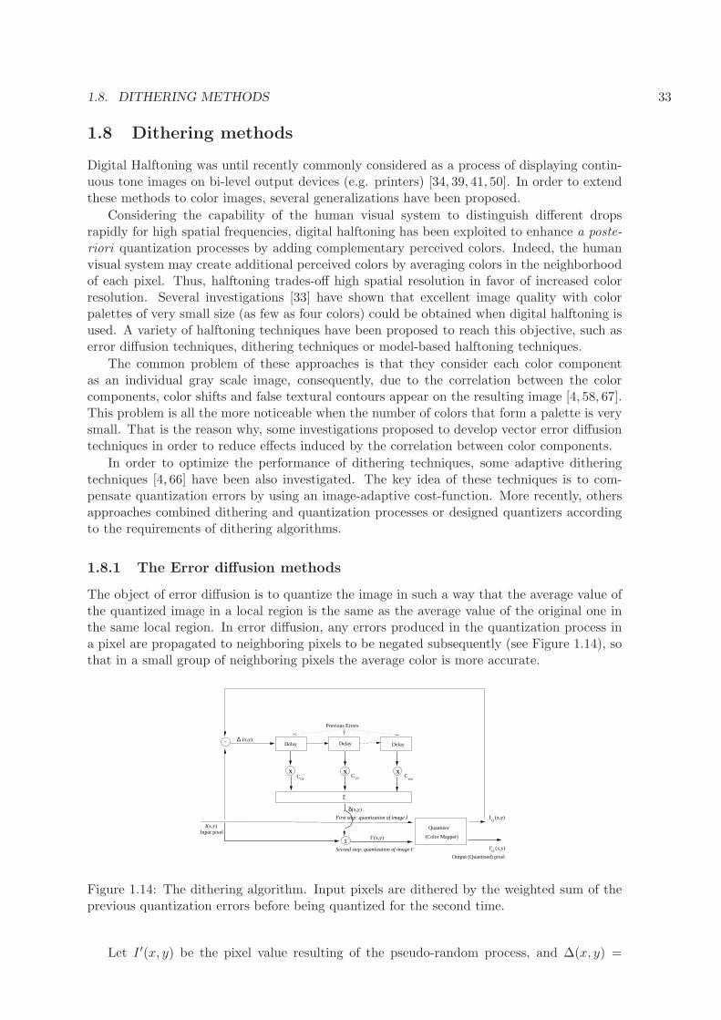
1.8. DITHERING METHODS 33
1.8 Dithering methods
Digital Halftoning was until recently commonly considered as a process of displaying contin-uous tone images on bi-level output devices (e.g. printers) [34, 39, 41, 50]. In order to extendthese methods to color images, several generalizations have been proposed.
Considering the capability of the human visual system to distinguish different dropsrapidly for high spatial frequencies, digital halftoning has been exploited to enhance a poste-riori quantization processes by adding complementary perceived colors. Indeed, the humanvisual system may create additional perceived colors by averaging colors in the neighborhoodof each pixel. Thus, halftoning trades-off high spatial resolution in favor of increased colorresolution. Several investigations [33] have shown that excellent image quality with colorpalettes of very small size (as few as four colors) could be obtained when digital halftoning isused. A variety of halftoning techniques have been proposed to reach this objective, such aserror diffusion techniques, dithering techniques or model-based halftoning techniques.
The common problem of these approaches is that they consider each color componentas an individual gray scale image, consequently, due to the correlation between the colorcomponents, color shifts and false textural contours appear on the resulting image [4, 58, 67].This problem is all the more noticeable when the number of colors that form a palette is verysmall. That is the reason why, some investigations proposed to develop vector error diffusiontechniques in order to reduce effects induced by the correlation between color components.
In order to optimize the performance of dithering techniques, some adaptive ditheringtechniques [4, 66] have been also investigated. The key idea of these techniques is to com-pensate quantization errors by using an image-adaptive cost-function. More recently, othersapproaches combined dithering and quantization processes or designed quantizers accordingto the requirements of dithering algorithms.
1.8.1 The Error diffusion methods
The object of error diffusion is to quantize the image in such a way that the average value ofthe quantized image in a local region is the same as the average value of the original one inthe same local region. In error diffusion, any errors produced in the quantization process ina pixel are propagated to neighboring pixels to be negated subsequently (see Figure 1.14), sothat in a small group of neighboring pixels the average color is more accurate.
−
X X X
Delay Delay Delay
Previous Errors
(x,y)∆
I(x,y)
δ(x,y)
Σ
Input pixel
Second step: quantization of image I’
First step: quantization of image I
(Color Mapper)
Quantizer
Σ
C C C01 10 mn
I’(x,y)
I (x,y)Q
Output (Quantized) pixel
I’ (x,y)Q
Figure 1.14: The dithering algorithm. Input pixels are dithered by the weighted sum of theprevious quantization errors before being quantized for the second time.
Let I ′(x, y) be the pixel value resulting of the pseudo-random process, and ∆(x, y) =
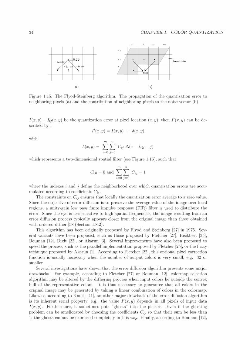
34 CHAPTER 1. COLOR QUANTIZATION
− ∆
− ∆ − ∆
− ∆ . 7/16
. /16
. 3/16
. 5/16 x
x−1
y−1 y y+2y+1
x−2
I(x,y)
Support region
a) b)
Figure 1.15: The Flyod-Steinberg algorithm. The propagation of the quantization error toneighboring pixels (a) and the contribution of neighboring pixels to the noise vector (b)
I(x, y) − IQ(x, y) be the quantization error at pixel location (x, y), then I ′(x, y) can be de-scribed by :
I ′(x, y) = I(x, y) + δ(x, y)
with
δ(x, y) =m∑
i=0
n∑
j=0
Cij ∆(x− i, y − j)
which represents a two-dimensional spatial filter (see Figure 1.15), such that:
C00 = 0 and
m∑
i=0
n∑
j=0
Cij = 1
where the indexes i and j define the neighborhood over which quantization errors are accu-mulated according to coefficients Cij .
The constraints on Cij ensures that locally the quantization error average to a zero value.Since the objective of error diffusion is to preserve the average value of the image over localregions, a unity-gain low pass finite impulse response (FIR) filter is used to distribute theerror. Since the eye is less sensitive to high spatial frequencies, the image resulting from anerror diffusion process typically appears closer from the original image than those obtainedwith ordered dither [58](Section 1.8.2).
This algorithm has been originally proposed by Flyod and Steinberg [27] in 1975. Sev-eral variants have been proposed, such as those proposed by Fletcher [27], Heckbert [35],Bouman [12], Dixit [22], or Akarun [3]. Several improvements have also been proposed tospeed the process, such as the parallel implementation proposed by Fletcher [25], or the fuzzytechnique proposed by Akarun [1]. According to Fletcher [22], this optional pixel correctionfunction is usually necessary when the number of output colors is very small, e.g. 32 orsmaller.
Several investigations have shown that the error diffusion algorithm presents some majordrawbacks. For example, according to Fletcher [27] or Bouman [12], colormap selectionalgorithm may be altered by the dithering process when input colors lie outside the convexhull of the representative colors. It is thus necessary to guarantee that all colors in theoriginal image may be generated by taking a linear combination of colors in the colormap.Likewise, according to Knuth [41], an other major drawback of the error diffusion algorithmis its inherent serial property, e.g., the value I ′(x, y) depends in all pixels of input dataI(x, y). Furthermore, it sometimes puts “ghosts” into the picture. Even if the ghostingproblem can be ameliorated by choosing the coefficients Cij so that their sum be less than1; the ghosts cannot be exorcised completely in this way. Finally, according to Bouman [12],
1.8. DITHERING METHODS 35
when the error diffusion algorithm is used in conjunction with an unstructured color palette,it requires an exhaustive search of the closest representative (Section 1.7). Although somebasic improvements of the exhaustive search method (Section 1.7.1) this method remainscomputationally intensive.
1.8.2 The Ordered dither methods
The ordered dithering methods add a non-random patterns δ(i, j) to blocks of pixels I(x, y)before the quantization step. The quantized image I ′(x, y) is thus deduced from the originalone by :
I ′(x, y) = I(x, y) + δ(x mod n, y mod n)
where δ(i, j) is a n by nmatrix of dithering values. The matrix δ is designed to have a 0 averagevalue and an energy spectrum with a minimal energy at low spatial frequencies [41]. Theamplitude of the pattern is determined so that any area of constant color value is quantizedinto a variety of nearby color values, thereby breaking up regions of false contouring. Thisreduces the correlated error patterns that are characteristic of areas of false contouring.
In contrast with random dithering processes, the basic idea of ordered dither techniquesis to use a finite, deterministic, and localized threshold function to decrease the correlationof quantization errors. Likewise, in contrast with random dithering processes, ordered dithertechniques are image-adaptative, e.g. these techniques exploit the local characteristics of theimage to obtain improvements over a constant filter.
Several investigations have shown that the ordered dither algorithm presents some majordrawbacks. According to Bouman [12], the application of ordered dithering is complicated bythe non-uniform spread of colors within the palette. As the distance between nearby colorsmay vary significantly across the color space, it may be impossible to determine the amplitudewhich will sufficiently dither all areas of constant color value in the image without addingnoticeable noise to other areas. Bouman et al [12] have thus proposed some adjustmentsto improve this technique. Nevertheless, it has been shown that no ordered dither methodguarantees that after quantization the error spectrum remains concentrated at high spatialfrequencies.
According to Kim et al. [40], ordered dither methods have the disadvantage of producinga binary-recursive and computerized texture that is unfortunately unsuitable. Meanwhile theFlyod-Steinberg method has the disadvantage to produce intrusive and snake-like patternsthat are also unsuitable. They thus proposed the dot diffusion method which avoids bothunsuitable previous properties but combines the sharpness of the Flyod-Steinberg method andthe parallelism of the order dither method. According to Kim et al. dot diffusion methodshave the desired property but tend to blur the image in the edge regions through the diffusionof the quantization error. This last problem is solved by an activity-weighted dot diffusionmethod which divide the dithering process into two sub-processes, one dependent on theobject frequencies and one independent.
Another approach of ordered dithering technique has been proposed by Lin et al. [45] toenhance performance of compression schemes such as joint bilevel group (JPIG) techniques.The interest of this approach, based on a pixel interleaving (i.e. grouping pixels with similardithering thresholds) strategy, is that it could be also extended to quantization scheme.
1.8.3 Vector dither methods
The major drawback of scalar diffusion techniques is that the color components are anal-ysed independently while they are highly correlated. Indeed the natural ordering used byscalar quantizers is lost within the vector quantizers framework. Imposing an ordering, ororganization, on a vector quantizer requires careful considerations. Rather than defining an
36 CHAPTER 1. COLOR QUANTIZATION
ordering on vectors, some investigations proposed a two-stage approach. In the first stagethe original image is quantized by a scalar process and an error propagation mask is appliedto compensate the quantization errors. In the second stage, the color palette is ordered andthe resulting image is once again quantized by a vector process based on the ordered palette.Finally, an error propagation mask is used one more time to compensate the quantizationerrors. This approach has been used by Goldschneider et al. [33] to propose an embeddedmultilevel error diffusion technique.
Another strategy of vector error diffusion has been proposed by Akarun et al. [4]. Inthis paper, authors proposed two new adaptive diffusion techniques respectively based onvector and scalar diffusion, to correct the disturbing effects of error diffusion strategies. Theproposed adaptation criterion is based on the statistics of the quantization error obtainedfrom the dithered image. Rather than considering each color component as an individualgray scale image to obtain a scalar diffusion, Akarun et al. [4] proposed to use either theKarhunen-Loeve color coordinate system or a pseudo-Karhunen-Loeve system which providesbetter results than the two others scalar diffusion techniques.
1.8.4 Joint quantization and dithering methods
Instead of performing a posteriori the dithering process to eliminate contouring effects or otherdisturbing effects, some investigations combined the dithering and quantization processes.Since the error diffusion step changes pixel values after the quantization step, the set ofrepresentative designed by the quantizer is obviously not optimal in regards to the correctedimage.
A first attempt to design the set of representatives based on a dithering process has beenproposed by Akarun et al. [2]. Akarun’s method combines a tree-structured vector quantizer(Section 1.4.2) and a dithering process based on a controlled displacement of cluster centers.The key idea is to obtain a wider colorspace in order to obtain more quantization colors inthe color palette, and hence eliminate color impulses and false contours.
Another strategy consists to process a joint optimization of the selection of the represen-tatives and their locations in order to benefit from the spatial averaging performed by theHuman Visual System. Indeed as mentioned in Sections 1.5 and 1.8, one notable character-istic of the Human Visual System is the rapid drop of its capabilities to distinguish differentcolors for high spatial frequencies. This phenomenon creates additional perceived colors bya visual local averaging of the representatives. This effect is widely used by dithering tech-niques but can not be readily incorporated in usual quantization algorithms since the set ofrepresentatives is known only after the quantization step.
A joint optimisation of the selection of the representatives and their locations has beenproposed by Scheunders et al. [57]. This method combines a quantization process based ona competitive learning clustering technique and a dithering process based on a simple localerror diffusion technique. To take the error diffusion process into account, an objective errorfunction is firstly computed and next minimized thanks to a competitive learning schemewhich alternatively updates the palette colors in the color space and the color pixels in thecolor image.
Other authors [26, 54] use a model of the spatial averaging performed by the Human VisualSystem within the joint quantization scheme. This spatial averaging may be modeled by 3low pass filters [26, 51] (Wk)k∈1,2,3. Let us denote by Si,k the spatial support of filter Wk at
position i. Given an image I = (Ii)i∈1,...,N the kth component of the perceived image I isgiven by:
∀k ∈ 1, 2, 3 ∀i ∈ 1, . . . , N Ik(i) =∑
j∈Si,k
Wk(j)I(j)k
1.9. CONCLUSION AND PERSPECTIVES 37
Given a set of representatives c1, . . . , cK, the location of each representative may be encodedby a N ×K Boolean matrix such that M(i, j) equals 1 if the pixel Ii is mapped to cj and 0otherwise. Using the K× 3 vector R of representatives such that R(i, k) is the kth coordinateof ci, the output image IQ is defined as:
∀i ∈ 1, . . . , N IQ(i) = M(i, .)R
where M(i, .) denotes the ith line of matrix M .
The perceived output image IQ is then given by:
∀k ∈ 1, 2, 3 ∀i ∈ 1, . . . , N IQ(i)k =∑
j∈Si,k
Wk(j)M(j, .)R(., k)
where R(., k) denotes the kth column of matrix R. Note that IQ(i)k = M(i, .)R(., k)
The distance between the perceived input and output images may then be defined as thesquared Euclidean distance between perceived colors:
H(M,R) =∑3
k=1
∑Ni=1
(
I(i)k − IQ(i)k
)2
=∑3
k=1
∑Ni=1
(
∑
j∈Si,kWk(j)I(j)k −
∑
j∈Si,kWk(j)M(j, .)R(., k)
)2
The minimization of the error H(M,R) requires thus to set both the matrices M and R. Aminimization of H(M,R) using a fixed value of R has been proposed by several halftoningmethods [26, 51]. However, a joint mimization of M and R has been proposed only recentlyby Puzicha [54] who uses an alternating minimization scheme: 1) Minimize H(M,R) withrespect to M keeping R fixed. 2) minimize H(M,R) with respect to R leaving M fixed. Thistwo step strategy is iterated until convergence. Each optimization step is performed by anannealing method whose convergence is accelerated by a hierarchical decomposition of theimage.
1.9 Conclusion and perspectives
This chapter has surveyed the current research on color quantization. Meanwhile significantgains in image quality may be obtained by researches on processing algorithms and displaytechniques, considerable improvements should result from researches on color metrics designedfor complex image scenes instead of the CIE metrics which are based on large uniform areas.That is, only few papers account for the perceptual aspects of color within quantizationalgorithms. Two strategies have nevertheless been investigated to extend the use of perceptualaspects within quantization algorithms.
The first strategy consists to use either a perceptually uniform or a luminance/chrominancecolor space. The main characteristic of a uniform color spaces is that the perceived differencebetween two colors is proportional to the Euclidean distance between their representations inthe uniform color space. A number of such spaces such as the CIELAB color space whichachieves this objective to varying degrees have been used in color image quantization [29].Most of uniform color spaces are also based on a luminance/chrominance separation. Some in-vestigations [29, 38, 54] studded the influence of the color space on the quality of the quantizedimages. However, none of these study exhibited one color space having definitive advantageswithin the quantization framework.
The second strategy consists to use spatio-color parameters which enable either to compen-sate a posteriori the main visible degradations between the original image and the quantizedone or to minimize a priori the number of visible degradations which may appear on the
38 CHAPTER 1. COLOR QUANTIZATION
quantized image in regards to the original image. The strategy which minimizes a priorithe spatio-color distortions should obviously be the best one. However, quantization algo-rithms using this strategy are generally computationally intensive. Moreover the design ofanalytic measures taking into account all visual distortions of a quantized image is still anopen problem.
Image context playing an important role in human color vision, the use of an uniform colorspace is not sufficient to quantify perceptual color distance. Likewise, the relative positionsof different colors in the image plane greatly influence our color interpretation. In orderto handle this characteristic of the human visual system, several approaches such as thosedescribed in Section 1.5 have integrated a color activity criterion into the quantization scheme.Unfortunately, such approaches remain highly heuristic, and far from offering a mathematicalmodel for context dependency of colors, to be integrated into as an objective function to aquantization process [40, 74]. In this context, color appearance models may appear promising.However, most of them are fairly complex and their suitability for color imaging remains to becomprehensively evaluated [58]. The development of simple models, more adapted to compleximage scenes is a promising challenge for color imaging applications [62].
Bibliography
[1] L. Akarun, D. Ozdemir, and E. Alpaydin. Fuzzy error diffusion of color images. In IEEEProcessing, pages 46–49, 1997.
[2] L. Akarun, D. Ozdemir, and O. Yalcin. Joint quantization and dithering of color images.In Proceedings of IEEE, pages 557–560, 1996. ICIP’96.
[3] L. Akarun, Y. Yardimci, and A. E. Cetin. Adaptive methods for dithering color images.In Proceedings of IEEE, pages 125–128, 1995.
[4] L. Akarun, Y. Yardlmcl, and A. E. Cetin. Adaptive methods for dithering color images.IEEE Transactions on Image Processing, 6(7):950–955, July 1997.
[5] M. E. Anderberg. Cluster analysis for applications. Academic Press, New York, 1973.
[6] F. Aurenhammer. Voronoi diagrams: a survey of fundamental geometric data structure.ACM Computing surveys, 33(3):345–405, 1991.
[7] R. Balasubramaian and J. Allebach. A New Approach to Palette Selection for ColorImages. Journal of Imaging Technology, 17(6):284–290, December 1991.
[8] R. Balasubramaian, J. Allebach, and C. A. Bouman. Color-Image Quantization withUse of a Fast Binary Splitting Technique. Journal of the Optical Society of America,11(11):2777–2786, November 1994.
[9] R. Balasubramaian, C. A. Bouman, and J. Allebach. Sequential Scalar Quantization ofColor Images. Journal of Electronic Imaging, 3(1):45–59, 1994.
[10] R. Balasubramanian and J. Allebach. A New Approach to Palette Selection for ColorImages. Human Vision, Visual Processing, and Digital Display III (1991), SPIE 1453:58–69, 1991.
[11] J. L. Bentley, J. H. Friedman, and R. A. Finkel. An algorithm for finding best matchesin logarithmic expected time. ACM Trans. Math. Software, 3:209–226, September 1977.
[12] C. Bouman and M. Orchard. Color Image Display with a Limited Palette Size. VisualCommunications and Image Processing IV (1989), SPIE 1199:522–533, 1989.
[13] C. Bouman and M. Orchard. Color Quantization of Images. IEEE Transactions onSignal Processing, 39(12):2677–2690, December 1991.
[14] J. P. Braquelaire and L. Brun. Comparison and optimization of methods of color imagequantization. IEEE Transactions on Image Processing, 6(7):1048–1052, july 1997.
[15] G. Braudaway. In A Procedure for Optimum Choice of a Small Number of Colors froma Large Color Palette for Color Imaging, pages 75–79, November 1986.
39
40 BIBLIOGRAPHY
[16] L. Brun. Segmentation d’images couleur a base Topologique. PhD thesis, UniversiteBordeaux I, 351 cours de la Liberation 33405 Talence, December 1996.
[17] L. Brun and M. Mokhtari. Two high speed color quantization algorithms. In cepadueseditions, editor, Proceedings of CGIP’2000, pages 116–121, Saint Etienne, October 2000.
[18] L. Brun and C. Secroun. A fast algorithm for inverse color map computation. ComputerGraphics Forum, 17(4):263–271, DECEMBER 1998. email me to obtain the article.
[19] M. Celenk. A color clustering technique for image segmentation. Computer Vision,Graphics, and Image Processing, 52:145–170, 1990.
[20] C. A. Chaudhuri, W. T. Chen, and J. Wang. A modified metric to compute distance.Pattern Recognition, 7(25):667–677, 1992.
[21] P. A. Chou, L. T., and G. R. M. Optimal pruning with applications to tree-structuredsource coding and modeling. IEEE Trans. Inf. Theory, 2:299–315, 1989.
[22] S. S. Dixit. Quantization of Color Images for Display/Printed on Limited Color OutputDevices. Computers and Graphics, 15(4):561–568, 1991.
[23] W. H. Equitz. A new vector quantization clustering algorithm. IEEE transactions onacoustics, speech, and signal processing, 37(10):1568–1575, october 1989.
[24] Y. S. Feng and N. M. Nasrabadi. Dynamic address-vector quantization of rgb colourimages. IEEE Proceedings, 138(4):225–???, August 1991.
[25] P. Fletcher. A SIMD Parallel Colour Quantization Algorithm. Computers & Graphics,15(3):365–373, 1991.
[26] T. J. Flohr, B. W. Kolpatzik, R. Balasubramanian, D. A. Carrara, C. A. Bouman,and J. P. Allebach. Model Based Color Image Quantization. Human Vision, VisualProcessing, and Digital Display IV (1993), SPIE 1913:270–281, 1993.
[27] R. W. Flyod and L. Steinberg. An adptative algorithm for spatial gray scale. In SID,editor, Int. Symp. Dig. Tech. Papers, volume 36, 1975.
[28] C. Froidevaux, M.-C. Gaudel, and M. Soria. Types de donnees et algorithmes. McGraw-Hill, 1990.
[29] R. Gentile, J. Allebach, and E. Walowit. Quantization of Color Images Based on UniformColor Spaces. Journal of Imaging Technology, 16(1):11–21, February 1990.
[30] A. Gersho and R. M. Gray. Vector Quantization and Signal Compression. KluwerAcademic Publishers, Norwel, 1991.
[31] M. Gervautz and W. Purgathofer. A Simple Method for Color Quantization: OctreeQuantization. In N. Magnenat-Thalmann and D. Thalmann, editors, New Trends inComputer Graphics, pages 219–231. Springer-Verlag, New York, NY, 1988.
[32] N. Goldberg. Colour Image Quantization for High Resolution Graphics Display. Imageand Vision Computing, 9(1):303–312, 1991.
[33] J. R. Goldschneider, E. A. Riskin, and P. W. Wong. Embedded mutilevel error diffusion.IEEE Transactions on Image Processing, 6(7):956–964, July 1997.
BIBLIOGRAPHY 41
[34] J. Gomes and L. Velho. Image processing for computer graphics, chapter Digital halfton-ing. Springer Verlag, 1997.
[35] P. S. Heckbert. Color Image Quantization for Frame Buffer Display. ACM ComputerGraphics (ACM SIGGRAPH ’82 Proceedings), 16(3):297–307, 1982.
[36] M. H. Hodgson. Reducing the computation requirements of the minimum distance clas-sifier. Remote sencing of Environnement, 25:117–128, 1988.
[37] G. Houle and E. Dubois. Quantization of Color Images for Display on Graphics Ter-minals. Proc. IEEE Global Telecommunications Conference (GLOBE COM ’86), pages284–297, December 1986.
[38] A. K. Jain and W. K. Pratt. Color Image Quantization. National TelecommunicationsConference 1972 Record, December 1972.
[39] J. F. Jarvis, C. N. Judice, and W. H. Ninke. A survey of techniques for the display ofcontinuous tone pictures on bilevel displays. Computer Graphics and Image Processing,4:13–40, 1976.
[40] K. M. Kim, C. S. Lee, E. J. Lee, and Y. H. Ha. Color image quantization and ditheringmethod based on visual system characteristics. Journal of Imaging Science and technol-ogy, 40(6):502–509, Nov. 1996.
[41] D. E. Knuth. Digital halftones by dots diffusion. ACM Transactions on Graphics,6(4):245–273, 1987.
[42] B. J. Kurz. Optimal Color Quantization for Color Displays. IEEE Computer Vision andPattern Recognition Proceedings, pages 217–224, January 1983.
[43] Y. W. Lim and S. U. Lee. On the color image segmentation algorithm based on thethresholding and the fuzzy c-means techniques. Pattern Recognition, 23(9):935–952,1990.
[44] J. Lin, J. Storer, and M. Cohn. On the complexity of the optimal tree pruning for sourcecoding. In Proc. of data compression conference, pages 63–72. IEEE computer societyPress Los Angeles, 1991.
[45] Y. Lin, Y. Wang, and T. H. Fan. Compaction of ordered dithered images with arithmeticcoding. IEEE Transaction on Image Processing, 10(5):797–802, may 2001.
[46] Y. Linde, A. Buzo, and R. Gray. An algorithm for vector quantizer design. IEEE Trans.Commun., 1:84–95, january 1980. COM-28.
[47] S. P. Llyod. Least squares quantization. IEEE Trans., pages 129–137, 1982. IT-28.
[48] Y.-I. Ohta, T. Kanade, and T. Sakai. Color information for region segmentation. Com-puter Vision, Graphics, and Image Processing, 13:222–241, 1980.
[49] A. W. Paeth. Mapping RGB Triples Onto Four Bits. In A. S. Glassner, editor, GraphicsGems, pages 233–245, 718. Academic Press Professional, Cambridge, MA, 1990.
[50] T. Pappas. Model-based halftoning of color images. IEEE Transactions on Image Pro-cessing, 6(7):1014–1024, July 1997.
[51] T. Pappas. Model based halftoning of color images. IEEE Trans. Image Processing,6:1014–1024, July 1997.
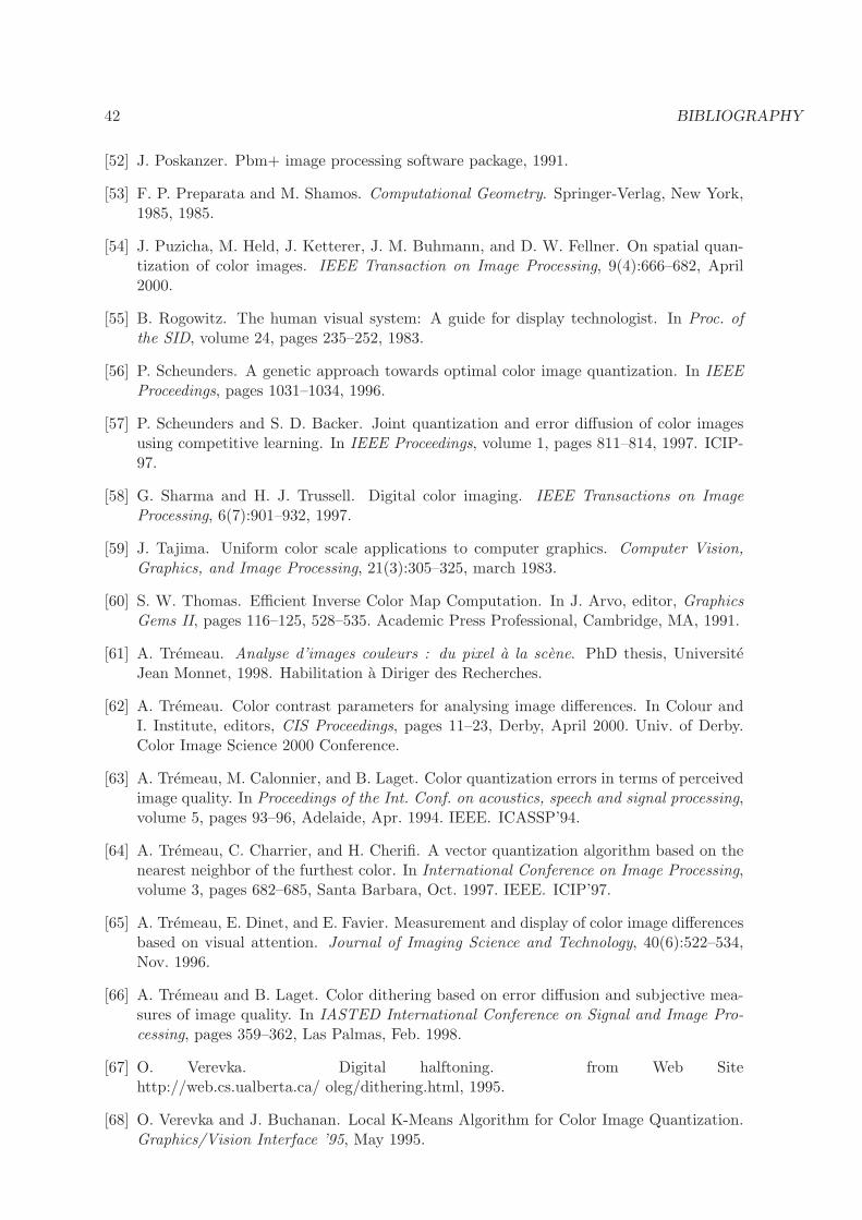
42 BIBLIOGRAPHY
[52] J. Poskanzer. Pbm+ image processing software package, 1991.
[53] F. P. Preparata and M. Shamos. Computational Geometry. Springer-Verlag, New York,1985, 1985.
[54] J. Puzicha, M. Held, J. Ketterer, J. M. Buhmann, and D. W. Fellner. On spatial quan-tization of color images. IEEE Transaction on Image Processing, 9(4):666–682, April2000.
[55] B. Rogowitz. The human visual system: A guide for display technologist. In Proc. ofthe SID, volume 24, pages 235–252, 1983.
[56] P. Scheunders. A genetic approach towards optimal color image quantization. In IEEEProceedings, pages 1031–1034, 1996.
[57] P. Scheunders and S. D. Backer. Joint quantization and error diffusion of color imagesusing competitive learning. In IEEE Proceedings, volume 1, pages 811–814, 1997. ICIP-97.
[58] G. Sharma and H. J. Trussell. Digital color imaging. IEEE Transactions on ImageProcessing, 6(7):901–932, 1997.
[59] J. Tajima. Uniform color scale applications to computer graphics. Computer Vision,Graphics, and Image Processing, 21(3):305–325, march 1983.
[60] S. W. Thomas. Efficient Inverse Color Map Computation. In J. Arvo, editor, GraphicsGems II, pages 116–125, 528–535. Academic Press Professional, Cambridge, MA, 1991.
[61] A. Tremeau. Analyse d’images couleurs : du pixel a la scene. PhD thesis, UniversiteJean Monnet, 1998. Habilitation a Diriger des Recherches.
[62] A. Tremeau. Color contrast parameters for analysing image differences. In Colour andI. Institute, editors, CIS Proceedings, pages 11–23, Derby, April 2000. Univ. of Derby.Color Image Science 2000 Conference.
[63] A. Tremeau, M. Calonnier, and B. Laget. Color quantization errors in terms of perceivedimage quality. In Proceedings of the Int. Conf. on acoustics, speech and signal processing,volume 5, pages 93–96, Adelaide, Apr. 1994. IEEE. ICASSP’94.
[64] A. Tremeau, C. Charrier, and H. Cherifi. A vector quantization algorithm based on thenearest neighbor of the furthest color. In International Conference on Image Processing,volume 3, pages 682–685, Santa Barbara, Oct. 1997. IEEE. ICIP’97.
[65] A. Tremeau, E. Dinet, and E. Favier. Measurement and display of color image differencesbased on visual attention. Journal of Imaging Science and Technology, 40(6):522–534,Nov. 1996.
[66] A. Tremeau and B. Laget. Color dithering based on error diffusion and subjective mea-sures of image quality. In IASTED International Conference on Signal and Image Pro-cessing, pages 359–362, Las Palmas, Feb. 1998.
[67] O. Verevka. Digital halftoning. from Web Sitehttp://web.cs.ualberta.ca/ oleg/dithering.html, 1995.
[68] O. Verevka and J. Buchanan. Local K-Means Algorithm for Color Image Quantization.Graphics/Vision Interface ’95, May 1995.
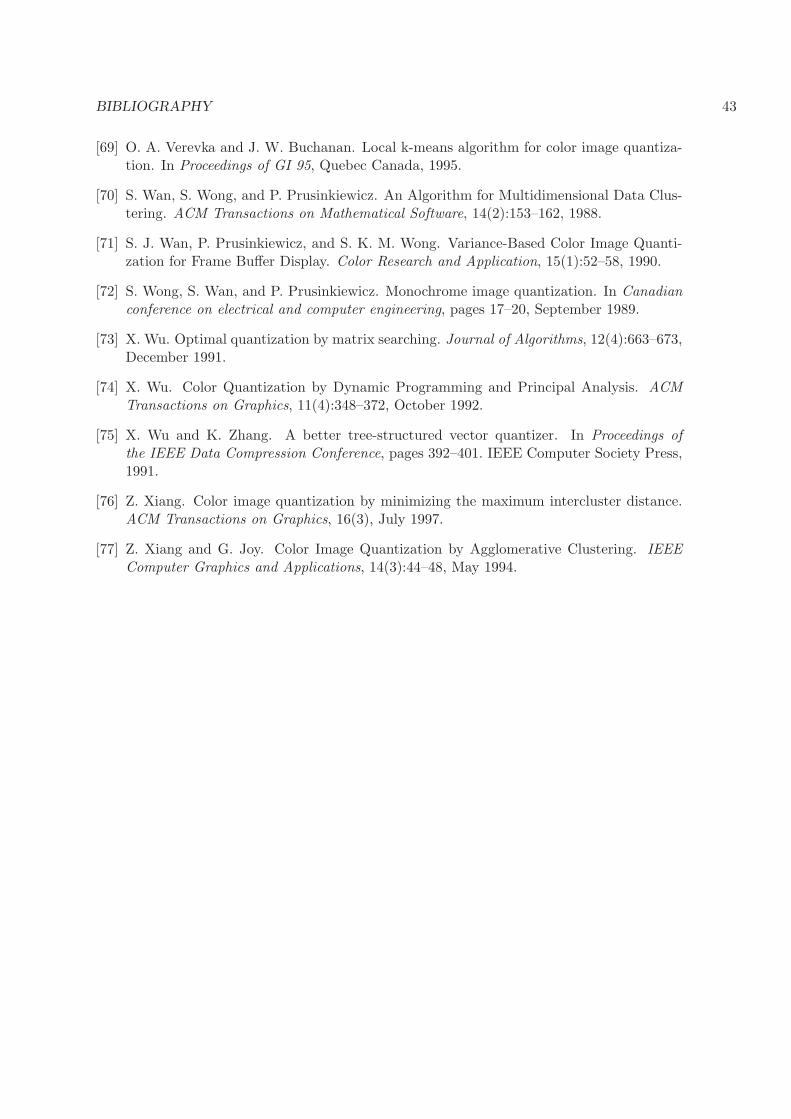
BIBLIOGRAPHY 43
[69] O. A. Verevka and J. W. Buchanan. Local k-means algorithm for color image quantiza-tion. In Proceedings of GI 95, Quebec Canada, 1995.
[70] S. Wan, S. Wong, and P. Prusinkiewicz. An Algorithm for Multidimensional Data Clus-tering. ACM Transactions on Mathematical Software, 14(2):153–162, 1988.
[71] S. J. Wan, P. Prusinkiewicz, and S. K. M. Wong. Variance-Based Color Image Quanti-zation for Frame Buffer Display. Color Research and Application, 15(1):52–58, 1990.
[72] S. Wong, S. Wan, and P. Prusinkiewicz. Monochrome image quantization. In Canadianconference on electrical and computer engineering, pages 17–20, September 1989.
[73] X. Wu. Optimal quantization by matrix searching. Journal of Algorithms, 12(4):663–673,December 1991.
[74] X. Wu. Color Quantization by Dynamic Programming and Principal Analysis. ACMTransactions on Graphics, 11(4):348–372, October 1992.
[75] X. Wu and K. Zhang. A better tree-structured vector quantizer. In Proceedings ofthe IEEE Data Compression Conference, pages 392–401. IEEE Computer Society Press,1991.
[76] Z. Xiang. Color image quantization by minimizing the maximum intercluster distance.ACM Transactions on Graphics, 16(3), July 1997.
[77] Z. Xiang and G. Joy. Color Image Quantization by Agglomerative Clustering. IEEEComputer Graphics and Applications, 14(3):44–48, May 1994.
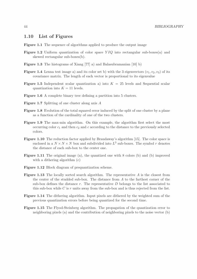
44 BIBLIOGRAPHY
1.10 List of Figures
Figure 1.1 The sequence of algorithms applied to produce the output image
Figure 1.2 Uniform quantization of color space Y IQ into rectangular sub-boxes(a) andskewed rectangular sub-boxes(b).
Figure 1.3 The histograms of Xiang [77] a) and Balasubramanian [10] b)
Figure 1.4 Lenna test image a) and its color set b) with the 3 eigenvectors (v1, v2, v3) of itscovariance matrix. The length of each vector is proportional to its eigenvalue
Figure 1.5 Independent scalar quantization a) into K = 25 levels and Sequential scalarquantization into K = 11 levels.
Figure 1.6 A complete binary tree defining a partition into 5 clusters.
Figure 1.7 Splitting of one cluster along axis A
Figure 1.8 Evolution of the total squared error induced by the split of one cluster by a planeas a function of the cardinality of one of the two clusters.
Figure 1.9 The max-min algorithm. On this example, the algorithm first select the mostoccurring color c1 and then c2 and c according to the distance to the previously selectedcolors.
Figure 1.10 The reduction factor applied by Braudaway’s algorithm [15]. The color space isenclosed in a N ×N ×N box and subdivided into L3 sub-boxes. The symbol r denotesthe distance of each sub-box to the center one.
Figure 1.11 The original image (a), the quantized one with 8 colors (b) and (b) improvedwith a dithering algorithm (c)
Figure 1.12 Block diagram of prequantization scheme.
Figure 1.13 The locally sorted search algorithm. The representative A is the closest fromthe center of the studded sub-box. The distance from A to the farthest corner of thesub-box defines the distance r. The representative D belongs to the list associated tothis sub-box while C is r units away from the sub-box and is thus rejected from the list.
Figure 1.14 The dithering algorithm. Input pixels are dithered by the weighted sum of theprevious quantization errors before being quantized for the second time.
Figure 1.15 The Flyod-Steinberg algorithm. The propagation of the quantization error toneighboring pixels (a) and the contribution of neighboring pixels to the noise vector (b)
Related Documents