Effects of Brand Preference, Product Attributes, and Marketing Mix Variables in Technology Product Markets S. Sriram ♣ Pradeep K. Chintagunta ♦ Ramya Neelamegham ♠ First Version: June 2004 Revised: September 2005 Forthcoming in Marketing Science ♣ School of Business, Uni versity of Connecti cut. [email protected] ♦ Graduate School of Business, Univers ity of Chicago. pradeep.chintagunta@gsb .uchicago.edu ♠ Amrita School of Business, India. [email protected] We thank the editor, area editor and two anonymous reviewers for their comments and suggestions. We also thank Sridhar Narayanan for help in conceptualizing our model specification and Bala Balachander, Manu Kalwani, Bill Robinson, Sriram Venkatraman, the seminar participants at the University of Connecticut, and the participants at the BCRST conference at Syracuse University for their comments and suggestions. This paper is based on one of the essays in the first author’s doctoral dissertati on. The second author thanks the Kilts’ Center for Marketing at the University of Chicago for financial support.

Welcome message from author
This document is posted to help you gain knowledge. Please leave a comment to let me know what you think about it! Share it to your friends and learn new things together.
Transcript
8/7/2019 Digicam Paper Final
http://slidepdf.com/reader/full/digicam-paper-final 1/38
Effects of Brand Preference, Product Attributes, and Marketing Mix Variables in
Technology Product Markets
S. Sriram
♣
Pradeep K. Chintagunta♦
Ramya Neelamegham♠
First Version: June 2004
Revised: September 2005
Forthcoming in Marketing Science
♣
School of Business, University of Connecticut. [email protected]♦ Graduate School of Business, University of Chicago. [email protected]♠ Amrita School of Business, India. [email protected]
We thank the editor, area editor and two anonymous reviewers for their comments and suggestions. We also thank Sridhar Narayanan for help in conceptualizing our model specification and Bala Balachander, Manu Kalwani, BillRobinson, Sriram Venkatraman, the seminar participants at the University of Connecticut, and the participants at theBCRST conference at Syracuse University for their comments and suggestions. This paper is based on one of theessays in the first author’s doctoral dissertation. The second author thanks the Kilts’ Center for Marketing at theUniversity of Chicago for financial support.
8/7/2019 Digicam Paper Final
http://slidepdf.com/reader/full/digicam-paper-final 2/38
Effects of Brand Preference, Product Attributes, and Marketing Mix Variables in
Technology Product Markets
Abstract
We develop a demand model for technology products that captures the effect of changes in the portfolioof models offered by a brand as well as the influence of the dynamics in its intrinsic preference on thatbrand’s performance. In order to account for the potential correlation in the preferences of modelsoffered by a particular brand, we use a nested logit model with the brand (e.g., Sony) at the upper leveland its various models (e.g., Mavica, FD, DSC, etc.) at the lower level of the nest. Relative modelpreferences are captured via their attributes and prices. We allow for heterogeneity across consumers intheir preferences for these attributes and in their price sensitivities in addition to heterogeneity inconsumers’ intrinsic brand preferences. Together with the nested logit assumption, this allows for aflexible substitution pattern across models at the aggregate level. The attractiveness of a brand’s product
line changes over time with entry and exit of new models and with changes in attribute and price levels.To allow for time-varying intrinsic brand preferences, we use a state-space model based on the Kalmanfilter, which captures the influence of marketing actions such as brand-level advertising on the dynamicsof intrinsic brand preferences. Hence, the proposed model accounts for the effects of brand preferences,model attributes and marketing mix variables on consumer choice. First, we carry out a simulation studyto ensure that our estimation procedure is able to recover the true parameters generating the data. Then,we estimate our model parameters on data for the U.S. digital camera market. Overall, we find that theeffect of dynamics in the intrinsic brand preference is greater than the corresponding effect of thedynamics in the brand’s product line attractiveness. Assuming plausible profit margins, we evaluate theeffect of increasing the advertising expenditures for the largest and the smallest brands in this categoryand find that these brands can increase their profitability by increasing their advertising expenditures. Wealso analyze the impact of modifying a camera model’s attributes on its profits. Such an analysis could
potentially be used to evaluate if product development efforts would be profitable.
Keywords: Econometric Models, Hi-Tech Marketing, Advertising, Product Line Attractiveness, ProductDevelopment, Nested Logit Models, Kalman Filter
8/7/2019 Digicam Paper Final
http://slidepdf.com/reader/full/digicam-paper-final 3/38
1
1. INTRODUCTION
Managers in many technology product-markets are faced with a variety of challenges. One
challenge is to monitor changes in consumer’s brand preferences over time. In practice, intrinsic
brand preferences can be inferred from tangible performance measures such as sales after accounting for
the effects of other factors that may have influenced these measures (e.g., Kamakura and Russell 1993).
Given the rapid introduction and withdrawal of models in these markets, one needs to, while measuring
the dynamics in brand preferences, partial out the effect of the changing portfolio of models on a brand’s
performance. For example, the introduction of the Mavica line of digital cameras by Sony helped it
obtain market leadership and the effect of such changes in product line need to be accounted for. Besides
monitoring these preference changes, managers are also interested in understanding the drivers of
preferences over time. For example, extant research (e.g., Jedidi, Mela, and Gupta 1999) recognizes the
importance of advertising in influencing brand preferences. Hence, managers may be interested in
understanding the role of advertising in driving the dynamics of brand preferences.
A second issue of interest to managers is to understand what drives the changes in a brand’s
performance over time. Given that the markets for technology products evolve rapidly, we usually
observe some interesting dynamics in the performance of the key brands. For example, in the context of
digital cameras, while Casio, the first brand to enter the market, moves from the position of market leader
at the beginning of the data to being the lowest selling brand at the end of the data, Sony registers a steady
increase in sales. As noted previously, one possibility is that changes in performance are tied to changes
in intrinsic preferences. At the same time, they could also be due to (a) the changing portfolio of models
in a brand’s product line; and / or (b) modifications in the attributes and prices of the models in the
product line. This calls for an assessment of the relative influence of product line and intrinsic brand
preferences on the performance of brands in a category. Such an assessment, will guide managers on
which aspect to emphasize in order to improve their brand’s performance.
Third, notwithstanding the rapid introduction and withdrawal of models and changing consumer
preferences, managers need to evaluate to effects of product attributes and marketing activities on the

8/7/2019 Digicam Paper Final
http://slidepdf.com/reader/full/digicam-paper-final 4/38
2
performance in the marketplace. A related issue is the need to assess the effects of attribute improvements
as well as the introduction of new models with enhanced product attributes on the performance of the
brand. Given the high cost of new product development (Urban and Hauser 1993), managers in
technology product-markets would like to quantify the potential benefits from developmental efforts
leading to attribute improvements so as to evaluate their feasibility.
In this paper, we develop a demand model for technology products that aims to address the above
issues. We model consumer choice of digital cameras at the brand-model level (for example, Sony
Mavica, Casio QV, etc.). A consumer’s utility for a model of digital camera is a function of the attributes
and the price of that model, with the consumer choosing the brand-model that maximizes utility or
deciding not to purchase in the product category. We account for the potential correlation in preferences
of models offered by a particular brand, using a nested logit model with the brand (e.g., Sony) at the
upper level and its various models (e.g., Mavica, FD, DSC, etc.) at the lower level of the nest. At the
aggregate level, we also allow for the potential correlation in utilities of digital camera models that share
similar attributes by allowing for consumer heterogeneity in attribute preferences. In addition, we allow
for heterogeneity in intrinsic brand preferences and in price sensitivities across consumers. We thus have
a demand model that provides flexible substitution patterns while being parsimonious. The inclusive
value across models in the nested logit reflects the attractiveness of the brand’s product line. This
attractiveness changes over time with entry and exit of models as well as due to changes in attribute and
price levels. Hence, brand-level preferences are driven by the inclusive value across models as well as the
intrinsic preferences for each of the brands.
To allow for time-varying intrinsic preferences at the brand level, we use a state-space model
based on the Kalman filter. This Kalman filter component captures the dynamics of the intrinsic brand
preferences as influenced by marketing actions such as advertising. In this way we allow for changing
brand preferences and can also understand the role that advertising plays in driving these preferences.
While the brand level of the model captures the dynamics in the inclusive value and the brand
preferences, the model choice part evaluates the tradeoffs consumers make between different attributes

8/7/2019 Digicam Paper Final
http://slidepdf.com/reader/full/digicam-paper-final 5/38
3
and thus enables us to quantify the consumer valuation of these attributes. For completeness, our model
specification also accounts for potential endogeneity in the pricing decisions of firms (Berry, Levinsohn,
and Pakes 1995; Sudhir 2001). We carry out a simulation study to ensure that our proposed estimation
procedure is able to recover the model parameters.
We estimate our model parameters on data for the U.S. digital camera market spanning 26
months from April 1997 through May 1999. Our results reveal that advertising influences brand
preferences for three out of the four brands. All the brands appear to have gained from the changes in
their product lines over time to varying degrees. We further investigate the extent to which each of the
brands relied on price reduction versus product innovations to make their product lines attractive. We
find that while a significant proportion of the gain due to product line changes may be attributed to
decreasing prices in case of Casio, majority of the gain for Sony was due to the introduction of models
with enhanced attributes. All brands except Casio also gain from increases in their intrinsic preferences.
Overall, we find that the effect of the dynamics in the intrinsic brand preferences is higher than the
corresponding effect of the dynamics in the product line for all the brands. Especially, the trends in the
sales of Casio and Sony are largely driven by the corresponding changes in brand preferences. Given
these results, we also assess the profitability of increasing advertising expenditures and changing product
attributes for various brand-models.
We provide an analysis of the robustness of our empirical results to alternative demand structures
that also result in flexible aggregate substitution pattern. In addition, we examine the sensitivity of our
empirical results to various model assumptions.
The rest of the paper is organized as follows. We first review research related to this paper. We
then present the demand model and discuss its estimation. Next, we describe the data. We then present
our empirical results based on the digital cameras category and discuss their implications. Subsequently,
we evaluate the appropriateness of alternative model specifications. Finally, we provide some concluding
comments.
8/7/2019 Digicam Paper Final
http://slidepdf.com/reader/full/digicam-paper-final 6/38
4
2. RELATED RESEARCH
Given our objectives of evaluating the effects of product attributes as well as capturing the
dynamics in the brand preferences on consumer choice, our paper is related to three streams of research.
The first stream pertains to studies that have modeled the effect of product attributes on consumer choice.
In the context of consumer-packaged goods, Fader and Hardie (1996) use household level scanner data to
model consumer choice amongst SKUs by projecting preferences on product attributes. In modeling
consumers’ choice of automobiles using aggregate data, Sudhir (2001) accounts for the effect of
automobile characteristics to estimate consumers’ preferences for these attributes. In this study, we use a
model that captures the effects of the various attributes of a brand of digital camera using aggregate data
in order to evaluate the impact of changes in these attributes on the brand’s performance.
The second stream studies the effect of a firm or a brand’s product line on its demand. Previous
research has established the relationship between a firm’s product line and the demand for its products,
especially with respect to the length of the product line. Studies by Kekre and Srinivasan (1990), Bayus
and Putsis (1999) and Draganska and Jain (2005a) find a positive impact of a firm’s product line length
(included as a covariate) on its demand. By contrast, as in Draganska and Jain (2005b), we explicitly
account for the influence of the attributes and prices of individual models in a brand’s product line (in
addition to the effect of the product line length) on that brand’s demand.
The third stream corresponds to those that model dynamic or time varying parameters. Jedidi,
Mela, and Gupta (1999) account for the effects of advertising and promotions on dynamic brand
preferences for packaged goods. Sudhir, Chintagunta, and Kadiyali (2005) model time-varying
competition and investigate the effects of the dynamics in competitive intensity on prices. Xie, Song,
Sirbu, and Wang (1997) and Putsis (1998) use a state-space model based on the Kalman filter (Hamilton
1994; Harvey 1990) to estimate time varying parameters in the context of new product sales.1
Neelamegham and Chintagunta (2004) estimate a dynamic linear model to capture the time varying
1 Other papers that have modeled dynamics using the Kalman filter include Naik, Mantrala, and Sawyer (1998),Akcura, Gonul, and Petrova (2004), and Naik, Raman, and Winer (2005).
8/7/2019 Digicam Paper Final
http://slidepdf.com/reader/full/digicam-paper-final 7/38
5
impact of product attributes at the brand-model level – similar to our unit of analysis. The focus of that
study is to obtain sales forecasts at the brand-model level. One limitation of that modeling approach that
is overcome by our proposed approach is that the presence of a large number of brand-models requires
aggregation of the data to the brand level for all models that are not the focus of the forecasting exercise.
By contrast, our model structure requires the presence of a few brands that are stable over time but that
could have several, time-varying numbers of model in their product lines. It is this feature that enables us
to use a state-space approach based on the Kalman filter to account for dynamic brand preferences.
3. MODEL AND ESTIMATION
During each period t , consumer h is faced with the decision of purchasing a digital camera
offered by one of the B brands that are in the market during that period or to not make a category
purchase, in which case, the consumer is said to have chosen the outside or no-purchase alternative.
Specifically, a consumer chooses to buy a model from the set of M bt = {1, 2, …, J bt } models offered by
brand b, b = 1, 2, …, B, where J bt is the number of models offered by brand b at time t . We represent the
consumer product choice behavior using the nested logit model. Under this approach the consumer’s
decision is a function of the consumer’s idiosyncratic needs, the preference for the brand, and the overall
attractiveness of the models offered by the brand. The indirect utility that household h derives from
model j offered by brand b at time t is given by
U hjbt = t + 0hbt + t b H θ + h X jbt + jbt ξ + (1-σ ) ehjbt + ehbt , (1)
where 0hbt is the household h’s intrinsic preference for the brand name b at time t , H bt is a vector of
environmental factors (such as holiday season2) that affect the utility of brand b, X jbt is the vector of
attributes of model j offered by brand b at time t such as resolution, maximum number of images that can
be stored, size of internal and external memory, type of storage media, size of the LCD and marketing
variables such as price, and h is the vector of consumer taste parameters corresponding to the product
attributes. In addition, X jbt may contain other factors such as the age of a model, which may have an
2 Although the presence of holidays may not be brand specific, we use the brand subscript for the environmentalfactors for the sake of generalizability.
8/7/2019 Digicam Paper Final
http://slidepdf.com/reader/full/digicam-paper-final 8/38
6
effect on the consumer’s perception of the model. In order to allow for the possibility that the age of a
model may have a non-linear effect on its utility, we include a quadratic term of this variable in the model
in addition to the linear term. As in most technology products, with the diffusion of the innovation, we
would expect some intrinsic category growth. The term t α is a time specific dummy, common to all
brands and relative to the outside good, that captures the intrinsic category growth in a flexible manner
without having to impose a specific functional form for such growth (e.g., via a linear and / or quadratic
trend term or via a Bass-type specification).3 The term jbt ξ captures the effect of omitted attributes such
as model color as well as other time varying brand-specific utility influencing factors that are observed by
the consumers but not by the researcher. It is assumed to have mean zero. The error term ehjbt is an i.i.d.
extreme value random error term that captures the idiosyncratic taste of household h for model j offered
by brand b at time t . The error term ehbt is the error component for all the models offered by brand b such
that (1-σ ) ehjbt + ehbt is also an extreme value random variable. The parameter σ (0 < σ < 1), which is the
scale parameter in the nested logit specification, captures the extent to which the utilities of the models
offered by a particular brand are correlated. Hence, the model in Equation 1 takes the specification of the
nested logit model with B+1 nests. For identification, we set the deterministic component of the utility of
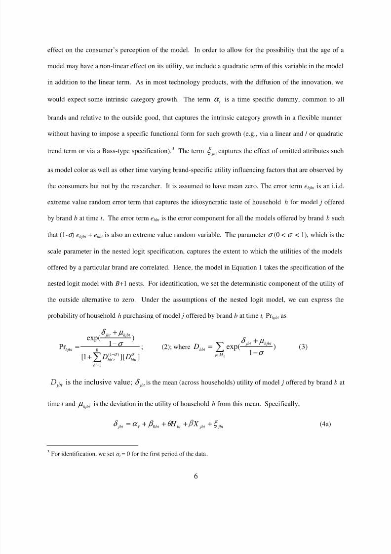
the outside alternative to zero. Under the assumptions of the nested logit model, we can express the
probability of household h purchasing of model j offered by brand b at time t, Prhjbt as
(1 )
'
' 1
exp( )1Pr ;
[1 ][ ]−
=
+
−=
+
jbt hjbt
hjbt B
hb t hbt
b
D Dσ σ
δ µ
σ (2); where ∈ −
+=
b M j
hjbt jbt
hbt D )1
exp(σ
µ δ (3)
is the inclusive value; jbt δ is the mean (across households) utility of model j offered by brand b at
time t and hjbt µ is the deviation in the utility of household h from this mean. Specifically,
jbt jbt bt bt jbt X H ξ θ β α δ τ ++++= 0 (4a)
3 For identification, we set t = 0 for the first period of the data.
8/7/2019 Digicam Paper Final
http://slidepdf.com/reader/full/digicam-paper-final 9/38
7
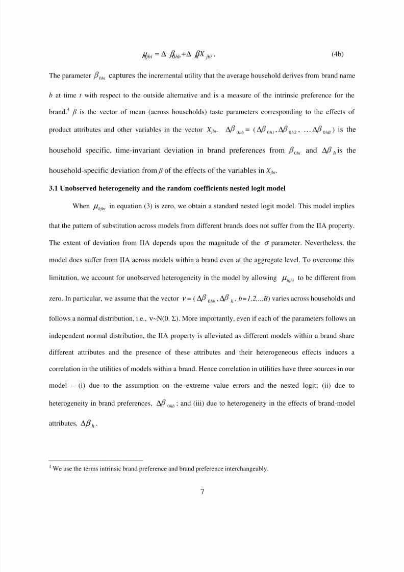
0= ∆ +∆hjbt hb h jbt X µ β β , (4b)
The parameter bt 0 captures the incremental utility that the average household derives from brand name
b at time t with respect to the outside alternative and is a measure of the intrinsic preference for the
brand.4 is the vector of mean (across households) taste parameters corresponding to the effects of
product attributes and other variables in the vector X jbt . 0hb∆ = ( 10h∆ , 20h∆ , … hB0∆ ) is the
household specific, time-invariant deviation in brand preferences from bt 0 and h∆ is the
household-specific deviation from of the effects of the variables in X jbt .
3.1 Unobserved heterogeneity and the random coefficients nested logit model
When hjbt µ in equation (3) is zero, we obtain a standard nested logit model. This model implies
that the pattern of substitution across models from different brands does not suffer from the IIA property.
The extent of deviation from IIA depends upon the magnitude of the σ parameter. Nevertheless, the
model does suffer from IIA across models within a brand even at the aggregate level. To overcome this
limitation, we account for unobserved heterogeneity in the model by allowing hjbt µ to be different from
zero. In particular, we assume that the vector ν = ( 0hb∆ , h∆ , b=1,2,..,B) varies across households and
follows a normal distribution, i.e., ν~N(0, Σ). More importantly, even if each of the parameters follows an
independent normal distribution, the IIA property is alleviated as different models within a brand share
different attributes and the presence of these attributes and their heterogeneous effects induces a
correlation in the utilities of models within a brand. Hence correlation in utilities have three sources in our
model – (i) due to the assumption on the extreme value errors and the nested logit; (ii) due to
heterogeneity in brand preferences, 0hb∆ ; and (iii) due to heterogeneity in the effects of brand-model
attributes, h β ∆ .
4 We use the terms intrinsic brand preference and brand preference interchangeably.
8/7/2019 Digicam Paper Final
http://slidepdf.com/reader/full/digicam-paper-final 10/38
8
Given the above distributional assumption on the vector, ν, the market share of model j offered
by brand b at time t, s jbt can be written as
(1 )
'' 1
exp( )
1 ( )[1 ][ ]
jbt hjbt
jbt B
Ahb t hbt
b
s D D
σ σ
δ µ
σ φ ν ν −
=
+
−= ∂+
, (4c)
In the above expression φ (.) denotes the density of a multivariate normal distribution and the region of
integration A is that which results in the choice of brand model jb. Hence our model described thus far is
a random coefficients nested logit model.
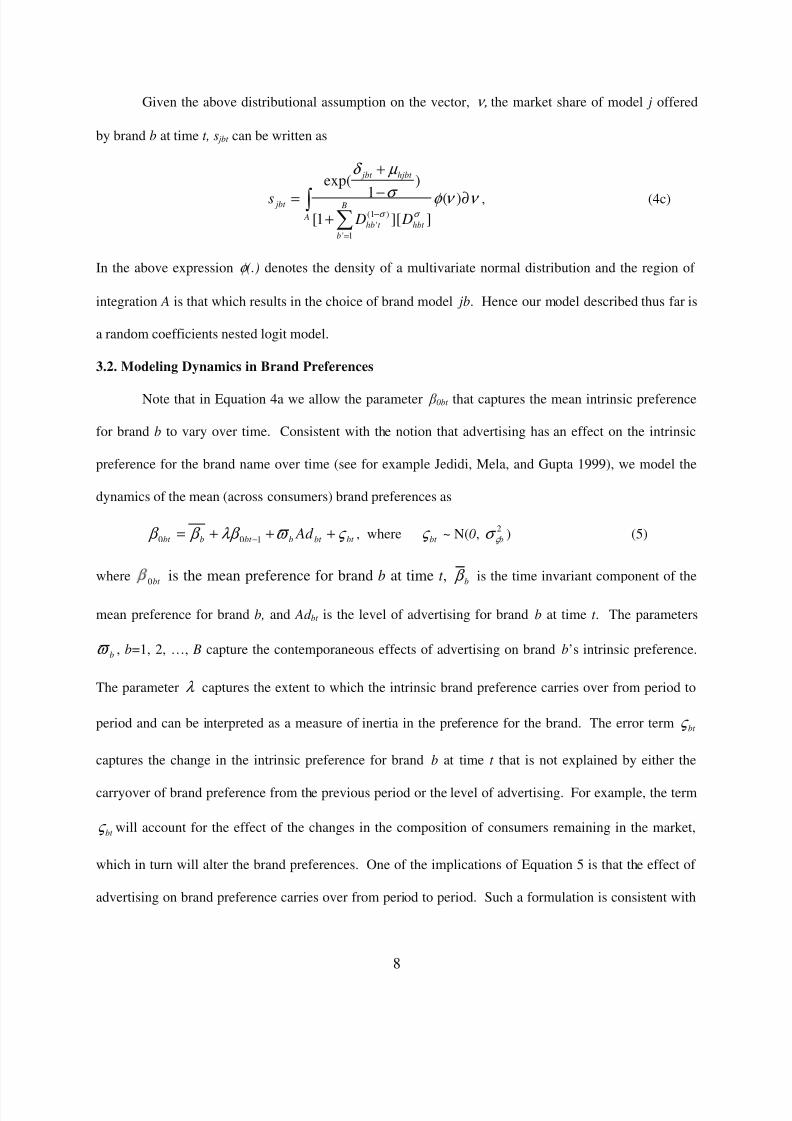
3.2. Modeling Dynamics in Brand Preferences
Note that in Equation 4a we allow the parameter 0bt that captures the mean intrinsic preference
for brand b to vary over time. Consistent with the notion that advertising has an effect on the intrinsic
preference for the brand name over time (see for example Jedidi, Mela, and Gupta 1999), we model the
dynamics of the mean (across consumers) brand preferences as
bt bt bbt bbt Ad ς ϖ λβ β β +++=−100 , where bt ς ~ N(0,
2bς σ ) (5)
where bt 0 is the mean preference for brand b at time t , b β is the time invariant component of the
mean preference for brand b, and Ad bt is the level of advertising for brand b at time t . The parameters
bϖ , b=1, 2, …, B capture the contemporaneous effects of advertising on brand b’s intrinsic preference.
The parameter λ captures the extent to which the intrinsic brand preference carries over from period to
period and can be interpreted as a measure of inertia in the preference for the brand. The error term bt ς
captures the change in the intrinsic preference for brand b at time t that is not explained by either the
carryover of brand preference from the previous period or the level of advertising. For example, the term
bt ς will account for the effect of the changes in the composition of consumers remaining in the market,
which in turn will alter the brand preferences. One of the implications of Equation 5 is that the effect of
advertising on brand preference carries over from period to period. Such a formulation is consistent with
8/7/2019 Digicam Paper Final
http://slidepdf.com/reader/full/digicam-paper-final 11/38
9
the finding that advertising has a long-term effect on brand preference (for example, Jedidi, Mela, and
Gupta 1999) and the extent of this carryover will depend on the magnitude of the parameter λ , with
higher values of λ implying a higher level of carryover and hence a higher level of persistence.
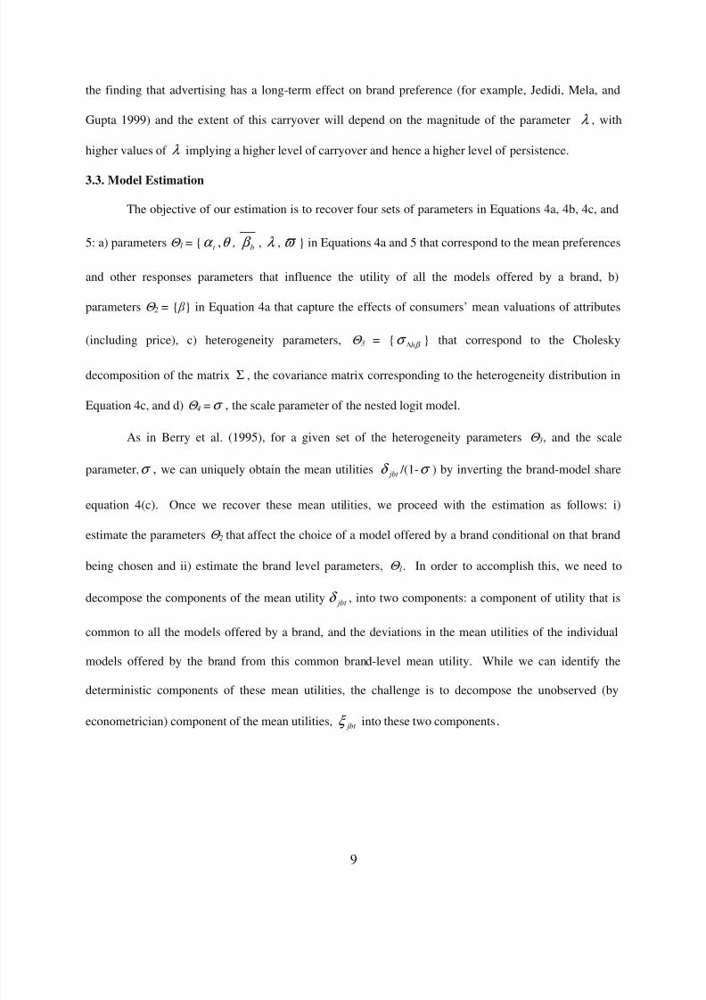
3.3. Model Estimation
The objective of our estimation is to recover four sets of parameters in Equations 4a, 4b, 4c, and
5: a) parameters Θ 1 = { t α ,θ , b β , λ , ϖ } in Equations 4a and 5 that correspond to the mean preferences
and other responses parameters that influence the utility of all the models offered by a brand, b)
parameters Θ 2 = { } in Equation 4a that capture the effects of consumers’ mean valuations of attributes
(including price), c) heterogeneity parameters, Θ 3 = { β σ h∆ } that correspond to the Cholesky
decomposition of the matrix Σ , the covariance matrix corresponding to the heterogeneity distribution in
Equation 4c, and d) Θ 4 =σ , the scale parameter of the nested logit model.
As in Berry et al. (1995), for a given set of the heterogeneity parameters Θ 3, and the scale
parameter,σ , we can uniquely obtain the mean utilities jbt δ /(1-σ ) by inverting the brand-model share
equation 4(c). Once we recover these mean utilities, we proceed with the estimation as follows: i)
estimate the parameters Θ 2 that affect the choice of a model offered by a brand conditional on that brand
being chosen and ii) estimate the brand level parameters, Θ 1. In order to accomplish this, we need to
decompose the components of the mean utility jbt δ , into two components: a component of utility that is
common to all the models offered by a brand, and the deviations in the mean utilities of the individual
models offered by the brand from this common brand-level mean utility. While we can identify the
deterministic components of these mean utilities, the challenge is to decompose the unobserved (by
econometrician) component of the mean utilities, jbt ξ into these two components.

8/7/2019 Digicam Paper Final
http://slidepdf.com/reader/full/digicam-paper-final 12/38
10
Recall that the term jbt ξ in the expression for jbt δ in Equation 4a captures the effect of omitted
attributes such as model color as well as other time varying brand-specific factors that are observed by the
consumers and may influence their utility of the models offered by the brand. We express jbt ξ as
jbt bt jbt ξ ξ ξ ∆+= , (6)
where bt ξ captures the unobserved factors common to all the models offered by brand b at time t and
jbt ξ ∆ is the corresponding model specific deviation for model j. Since our objective is to isolate the
dynamics in the intrinsic brand preferences, a key step in the estimation is to separate out these two
components of the unobserved error term jbt ξ . For purposes of identification, we need to set the model
specific deviation in the unobserved factors, jbt ξ ∆ , to 0 for one of the models of each brand. We do this
for a model that is available throughout the time series for each brand. We now discuss the estimation of
the parameters in i) and ii) above.
3.3.1. Estimating the Parameters that Affect Model Choice ( Θ ΘΘ Θ 2 )
Our identifying assumption that the model specific deviation in the unobserved factors, jbt ξ ∆ , is
equal to 0 for one model by each brand implies that we can write the mean utility of the base model of
brand b at time t as
bt bt bt bt t bt X H ξ θ α δ ++++= 101 , (7)
where the subscript 1 refers to the base model. Subtracting Equation (7) from Equation (4a) for all the
remaining models offered by brand b at time t , we have
jbt jbt jbt bt jbt X ξ δ δ δ ∆+∆==− '1 , j = 2, … J bt , (8)
where bt jbt jbt X X X 1−=∆ . Now in equation (8), the left hand side quantity is known since we have
already computed jbt δ by inverting the brand-model share equation 4(c). So the β (=Θ 2) parameters can
8/7/2019 Digicam Paper Final
http://slidepdf.com/reader/full/digicam-paper-final 13/38
11
be estimated via an instrumental variables regression that accounts for potential correlation between
jbt ξ ∆ and the prices embedded in
jbt X ∆ .
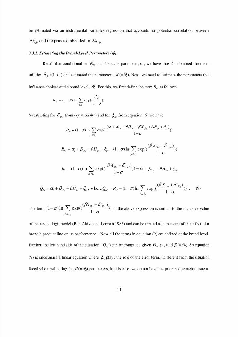
3.3.2. Estimating the Brand-Level Parameters ( Θ ΘΘ Θ 1 )
Recall that conditional on Θ 3, and the scale parameter,σ , we have thus far obtained the mean
utilities jbt δ /(1-σ ) and estimated the parameters, β (=Θ 2). Next, we need to estimate the parameters that
influence choices at the brand level, Θ ΘΘ Θ 1. For this, we first define the term Rbt as follows.
∈ −
−=
b M j
jbt
bt R ))
1exp((ln)1(
σ
δ σ
Substituting for jbt
δ from equation 4(a) and for jbt
ξ from equation (6) we have
0( )(1 ) ln exp(( ))
1b
t bt bt jbt jbt bt
bt
j M
H X R
α β θ β ξ ξ σ
σ ∈
+ + + + ∆ += −
−
1
0
( ' )(1 ) ln exp(( ))
1b
bt jbt
bt t bt bt bt
j M
X R H
δ α β θ ξ σ
σ ∈
+= + + + + −
−
1
0
( ' )(1 ) ln exp(( ))
1b
bt jbt
t t bt bt bt
j M
X R H
δ σ α β θ ξ
σ ∈
+− − = + + +
−
1
0
( ' ); where (1 ) ln exp(( ))
1b
bt jbt
bt t bt bt bt bt bt
j M
X Q H Q R
δ α β θ ξ σ
σ ∈
+= + + + = − −
− . (9)
The term ∈
−
+−
b M j
jbt bt X ))
1
)'(exp((ln)1(
1
σ
δ β σ in the above expression is similar to the inclusive value
of the nested logit model (Ben-Akiva and Lerman 1985) and can be treated as a measure of the effect of a
brand’s product line on its performance.
Now all the terms in equation (9) are defined at the brand level.
Further, the left hand side of the equation (t Q ) can be computed given Θ 3, σ , and β (=Θ 2). So equation
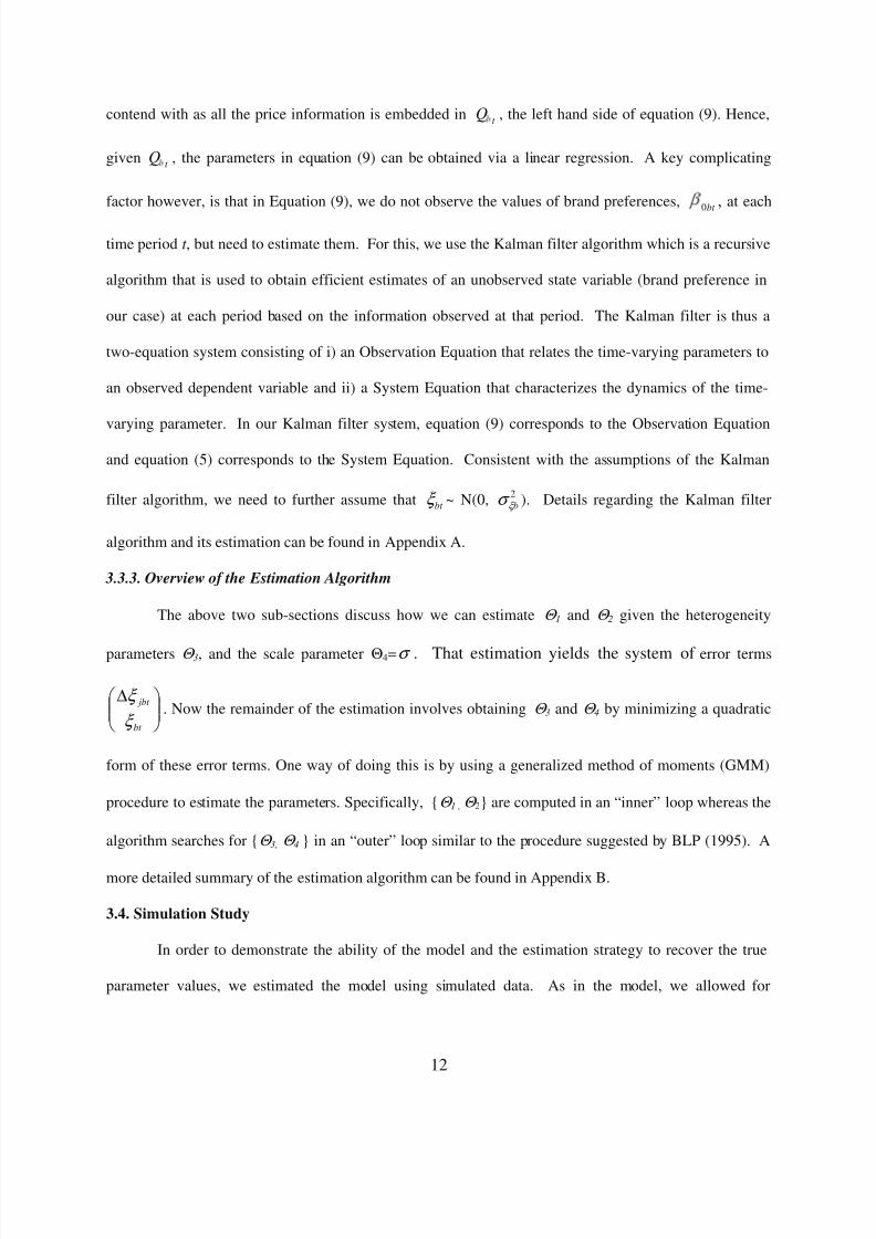
(9) is once again a linear equation where t ξ plays the role of the error term. Different from the situation
faced when estimating the β (=Θ 2) parameters, in this case, we do not have the price endogeneity issue to
8/7/2019 Digicam Paper Final
http://slidepdf.com/reader/full/digicam-paper-final 14/38
12
contend with as all the price information is embedded int Q , the left hand side of equation (9). Hence,
givent Q , the parameters in equation (9) can be obtained via a linear regression. A key complicating
factor however, is that in Equation (9), we do not observe the values of brand preferences, bt 0 , at each
time period t , but need to estimate them. For this, we use the Kalman filter algorithm which is a recursive
algorithm that is used to obtain efficient estimates of an unobserved state variable (brand preference in
our case) at each period based on the information observed at that period. The Kalman filter is thus a
two-equation system consisting of i) an Observation Equation that relates the time-varying parameters to
an observed dependent variable and ii) a System Equation that characterizes the dynamics of the time-
varying parameter. In our Kalman filter system, equation (9) corresponds to the Observation Equation
and equation (5) corresponds to the System Equation. Consistent with the assumptions of the Kalman
filter algorithm, we need to further assume that bt ξ ~ N(0,2bξ σ ). Details regarding the Kalman filter
algorithm and its estimation can be found in Appendix A.
3.3.3. Overview of the Estimation Algorithm
The above two sub-sections discuss how we can estimate Θ 1 and Θ 2 given the heterogeneity
parameters Θ 3, and the scale parameter Θ4=σ . That estimation yields the system of error terms
∆
bt
jbt
ξ
ξ . Now the remainder of the estimation involves obtaining Θ 3 and Θ 4 by minimizing a quadratic
form of these error terms. One way of doing this is by using a generalized method of moments (GMM)
procedure to estimate the parameters. Specifically, {Θ 1 , Θ 2} are computed in an “inner” loop whereas the
algorithm searches for {Θ 3, Θ 4 } in an “outer” loop similar to the procedure suggested by BLP (1995). A
more detailed summary of the estimation algorithm can be found in Appendix B.
3.4. Simulation Study
In order to demonstrate the ability of the model and the estimation strategy to recover the true
parameter values, we estimated the model using simulated data. As in the model, we allowed for

8/7/2019 Digicam Paper Final
http://slidepdf.com/reader/full/digicam-paper-final 15/38
13
consumer heterogeneity in the four brand preferences, resolution, and price. Further, we assumed that the
covariance matrix corresponding to the heterogeneity distribution of these six parameters had variances
equal to 2 and covariances equal to 1. The rest of the true parameter values were chosen to be the actual
estimates reported in Table 3 (to be discussed later). Using these parameter values and the actual price,
advertising, attributes, and holiday data from the digital camera category, we simulated the share data for
each of the brand-model combination for each of the 26 months as follows. As in the model (Equation 5),
we assumed that the brand preference was driven by advertising. In order to reflect the nested logit model
specification, the household specific idiosyncratic preferences were drawn from a generalized extreme
value (GEV) distribution. The aggregate shares were generated from 10,000 household level draws. We
estimated the model parameters using 25 replications of simulated data. In Table 2, we present a
summary of the implied elasticity estimates across these 25 replications. Overall the results reveal that
for the range of parameter values considered, the model and the estimation procedure can recover the true
elasticity values with a reasonable level of accuracy. Moreover, all the true elasticities are contained
within the 95% confidence interval of the estimates. 5
4. DATA DESCRIPTION AND OPERATIONALIZATION OF VARIABLES
4.1. Data
Our data consist of aggregate monthly observations on unit sales and prices of digital cameras
collected via store audits for a period of 26 months from April 1997 through May 1999. In addition, the
data consist of information on the features of each model marketed by the manufacturers in the category.
The features include, for example, the maximum resolution in mega pixels, maximum number of images
that can be stored, size of internal and external memory, type of storage media, and the presence or
absence of self-timer capabilities. We supplemented these with data on monthly advertising expenditures
by each of the brands during the corresponding period. The advertising data are obtained from
5 For a more detailed discussion of the simulation study as well as for a summary of the parameter estimates, pleaserefer to Appendix C posted on the first author’s website.

8/7/2019 Digicam Paper Final
http://slidepdf.com/reader/full/digicam-paper-final 16/38
14
Competitive Media Reporting. Hence, sales, price and attribute data are at the model level (Sony DSCF1)
whereas advertising data are at the brand level (i.e., for Sony across all its models).
We perform our empirical analysis on the four leading brands in this category – Casio, Kodak,
Olympus, and Sony. Together these brands account for over 93% of the sales in this category over the
time period and the four brands are present during all the 26 months of the data. We report the
descriptive statistics for the four brands in Table 1. From Table 1, we can see Sony has the highest
market share, which is almost twice that of the nearest competitor, Kodak. Olympus comes a close third
to Kodak in terms of market share and Casio has the lowest market share. Although Sony has the highest
market share, it also commands the highest price. In contrast, Casio, which has the lowest market share,
has the lowest average price. Sony’s high market share despite its high price may potentially be attributed
to the attractiveness of models in its product line and / or to a high intrinsic preference for the brand. It is
of substantive interest to investigate which of these two plays a more dominant role in Sony’s ability to
command a higher price. The total advertising expenditure of the brands provides some evidence for the
source of Sony’s success. Among the four brands, Sony had the highest advertising expenditure while
Casio had the lowest. In fact, Casio’s advertising expenditure was just 7% of that spent by Sony during
this period. Another reason for Sony’s success could be its introduction of models with a floppy disk
storage device. Its convenience revolutionized the digital camera market and was one of the reasons
behind Sony’s popularity despite bulkiness and higher price ( Business Week , Aug 14 2000).
We report the time trend in monthly sales of these brands over the 26 months in Figure 1. Figure
1 reveals that although Casio was the largest selling brand at the beginning of the data, its unit sales
steadily decreased over time and it ended up as the lowest selling brand. In contrast, although Sony has
the lowest market share in the first few months, it soon overtook all the other brands to emerge as the
largest selling brand. The other two brands, Kodak and Olympus exhibit a gradual increase in unit sales
over time. It will thus be interesting to investigate the reasons behind these contrasting trends in sales
and relative market shares of the various brands. As in most technology product markets, the average
price of the models sold by each of the brands declines over time. The decrease ranges from a high of
8/7/2019 Digicam Paper Final
http://slidepdf.com/reader/full/digicam-paper-final 17/38
15
48% for Sony to about 22% in case of Kodak. In addition, the number of models offered by each of the
brands steadily increases during this period.
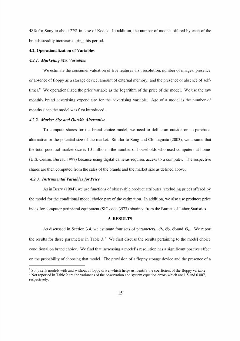
4.2. Operationalization of Variables
4.2.1. Marketing Mix Variables
We estimate the consumer valuation of five features viz., resolution, number of images, presence
or absence of floppy as a storage device, amount of external memory, and the presence or absence of self-
timer.6 We operationalized the price variable as the logarithm of the price of the model. We use the raw
monthly brand advertising expenditure for the advertising variable. Age of a model is the number of
months since the model was first introduced.
4.2.2. Market Size and Outside Alternative
To compute shares for the brand choice model, we need to define an outside or no-purchase
alternative or the potential size of the market. Similar to Song and Chintagunta (2003), we assume that
the total potential market size is 10 million – the number of households who used computers at home
(U.S. Census Bureau 1997) because using digital cameras requires access to a computer. The respective
shares are then computed from the sales of the brands and the market size as defined above.
4.2.3. Instrumental Variables for Price
As in Berry (1994), we use functions of observable product attributes (excluding price) offered by
the model for the conditional model choice part of the estimation. In addition, we also use producer price
index for computer peripheral equipment (SIC code 3577) obtained from the Bureau of Labor Statistics.
5. RESULTS
As discussed in Section 3.4, we estimate four sets of parameters, Θ 1 , Θ 2 , Θ 3 and Θ 4 .. We report
the results for these parameters in Table 3.7 We first discuss the results pertaining to the model choice
conditional on brand choice. We find that increasing a model’s resolution has a significant positive effect
on the probability of choosing that model. The provision of a floppy storage device and the presence of a
6 Sony sells models with and without a floppy drive, which helps us identify the coefficient of the floppy variable.7 Not reported in Table 2 are the variances of the observation and system equation errors which are 1.5 and 0.007,respectively.

8/7/2019 Digicam Paper Final
http://slidepdf.com/reader/full/digicam-paper-final 18/38
16
self-timer have similar effects. The significant positive effect of floppy storage is consistent with the
claim in the business press that Sony’s introduction of models with floppy as the storage device was a key
reason behind its success. As expected, we find that price has a negative effect on a model’s share.
While the coefficient of the linear age term is negative and significant, we find that the coefficient of the
quadratic term is positive but insignificant. These results imply that as the age of a model increases, it is
increasingly perceived as becoming obsolete.
We now discuss the brand choice results. Our estimates of the intrinsic growth parameters t α ,
which proxy for category diffusion are statistically indistinguishable from zero. Hence we do not
report those estimates here. Essentially, this finding implies that controlling for the changes in the product
line and the intrinsic brand preferences, effectively controls for growth in the category over the time range
of our data. The parameter λ that captures the carryover of brand preferences from period to period
(CARRYOVER) is 0.927. This is consistent with our expectation that the intrinsic brand preferences
should be highly persistent and should hence have a positive and high (close to 1) carryover. The high
carryover of the intrinsic brand preferences is consistent with the notion that “brand equity” is an
enduring construct (Keller 1998). The constant component of the intrinsic brand preferences that is
invariant to marketing actions is highest for Sony and lowest for Casio. Advertising has a significant
positive effect on the intrinsic brand preferences of Casio, Olympus, and Sony. Given that the carryover
coefficient is 0.927, the long-term effect of advertising is over 13 times the short-term month-level effect.
Hence, managers need to consider the total effect of advertising, particularly the long-term effect, while
evaluating the effectiveness of their advertising campaigns. The estimate of σ (0.9542), implies that the
correlation in the utilities of the models offered by the same brand is high.
As our approach explicitly accounts for all the models marketed by the competing brands, we
can compute the 46 x 46 matrix of cross price elasticities across all brand-models.8 However, for
illustrative purposes, we computed the model specific price elasticities for four select models (one for
8 The total number of models offered by the four brands during this period was 46. However, because of the entryand exit of models, the number of models available in the market during any period was less than 46.
8/7/2019 Digicam Paper Final
http://slidepdf.com/reader/full/digicam-paper-final 19/38
17
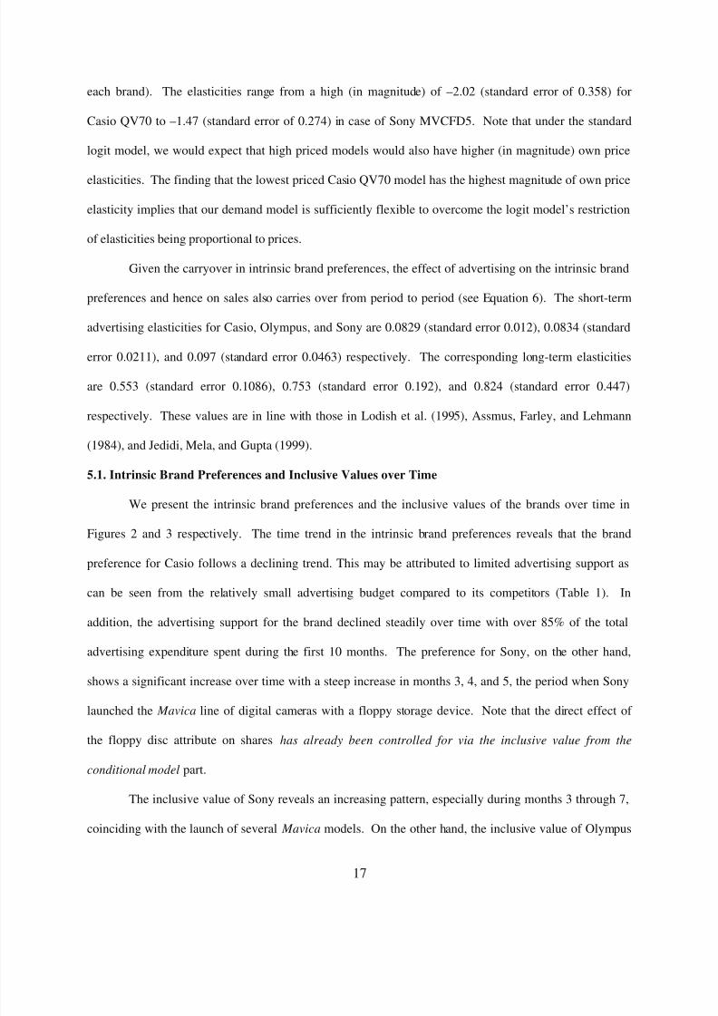
each brand). The elasticities range from a high (in magnitude) of –2.02 (standard error of 0.358) for
Casio QV70 to –1.47 (standard error of 0.274) in case of Sony MVCFD5. Note that under the standard
logit model, we would expect that high priced models would also have higher (in magnitude) own price
elasticities. The finding that the lowest priced Casio QV70 model has the highest magnitude of own price
elasticity implies that our demand model is sufficiently flexible to overcome the logit model’s restriction
of elasticities being proportional to prices.
Given the carryover in intrinsic brand preferences, the effect of advertising on the intrinsic brand
preferences and hence on sales also carries over from period to period (see Equation 6). The short-term
advertising elasticities for Casio, Olympus, and Sony are 0.0829 (standard error 0.012), 0.0834 (standard
error 0.0211), and 0.097 (standard error 0.0463) respectively. The corresponding long-term elasticities
are 0.553 (standard error 0.1086), 0.753 (standard error 0.192), and 0.824 (standard error 0.447)
respectively. These values are in line with those in Lodish et al. (1995), Assmus, Farley, and Lehmann
(1984), and Jedidi, Mela, and Gupta (1999).
5.1. Intrinsic Brand Preferences and Inclusive Values over Time
We present the intrinsic brand preferences and the inclusive values of the brands over time in
Figures 2 and 3 respectively. The time trend in the intrinsic brand preferences reveals that the brand
preference for Casio follows a declining trend. This may be attributed to limited advertising support as
can be seen from the relatively small advertising budget compared to its competitors (Table 1). In
addition, the advertising support for the brand declined steadily over time with over 85% of the total
advertising expenditure spent during the first 10 months. The preference for Sony, on the other hand,
shows a significant increase over time with a steep increase in months 3, 4, and 5, the period when Sony
launched the Mavica line of digital cameras with a floppy storage device. Note that the direct effect of
the floppy disc attribute on shares has already been controlled for via the inclusive value from the
conditional model part.
The inclusive value of Sony reveals an increasing pattern, especially during months 3 through 7,
coinciding with the launch of several Mavica models. On the other hand, the inclusive value of Olympus

8/7/2019 Digicam Paper Final
http://slidepdf.com/reader/full/digicam-paper-final 20/38
18
increases initially and drops marginally towards the end of the data. The inclusive value of Casio
decreases marginally during the period, with the value peaking during the 17 th month of the data. The
other brand, Kodak sees a steady increase in its inclusive value throughout the data.
The above patterns in the intrinsic brand preferences and the inclusive values raise an interesting
question: what is the effect of the dynamics in the intrinsic brand preferences on the sales of a brand
relative to that of the dynamics in the inclusive values? To answer this question, we performed two sets
of simulations for each brand. In the first simulation, we computed the market shares and the
corresponding sales of the brand if the intrinsic preference of the brand had been the same for the entire
period as in the first period. We then obtained the difference between the actual observed sales of the
brand and the simulated sales. The difference is a measure of the extra sales that can be attributed to the
dynamics in the intrinsic preference for the brand. A positive (negative) value of this measure at any
period will imply a positive (negative) effect of the dynamics in brand preference during that period. We
then performed the second simulation wherein the inclusive value of the brand was constrained to be the
same as that in the first period. Once again, the difference between the true sales and the simulated sales
can be attributed to the dynamics in the inclusive value.9
We present the total effect (both positive and negative) of these dynamics in terms of unit sales in
Table 4. The net effect of the dynamics is the sum of the positive and the negative effects. All the four
brands seem to have benefited from the increase in inclusive values over time. From Table 4, we can see
that Casio has gained the least at roughly 4,100 units over the 25 months.10 Sony, which seems to have
gained the most from the increase in its inclusive values, has gained roughly 15 times as much as Casio.
The remaining two brands, Kodak and Olympus seem to have gained approximately 8,400 and 12,400
units respectively in sales due to the dynamics in their inclusive values.
9 Note that because of the non-linear nature in which the utilities enter the demand equation, the effects of thedynamics in the inclusive value and the intrinsic brand preference are not additive.10 Since the values are fixed at the first month levels, we compute the effects for the remaining 25 months of thedata.
8/7/2019 Digicam Paper Final
http://slidepdf.com/reader/full/digicam-paper-final 21/38
19
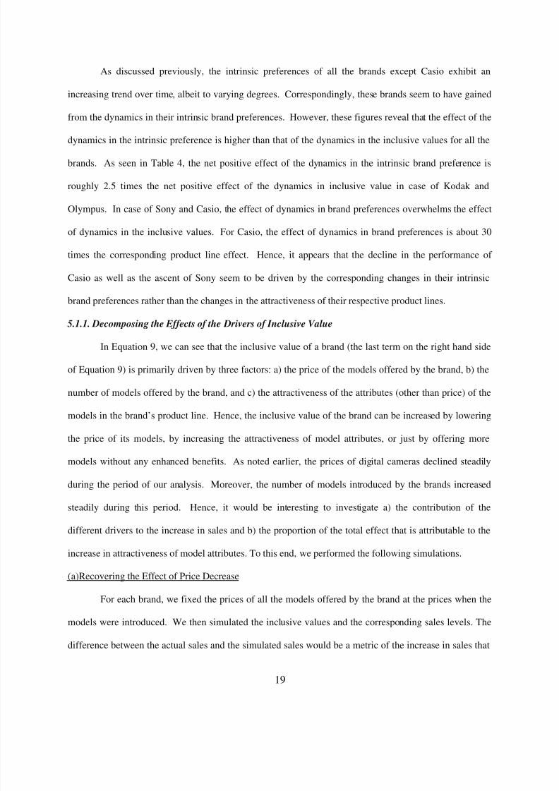
As discussed previously, the intrinsic preferences of all the brands except Casio exhibit an
increasing trend over time, albeit to varying degrees. Correspondingly, these brands seem to have gained
from the dynamics in their intrinsic brand preferences. However, these figures reveal that the effect of the
dynamics in the intrinsic preference is higher than that of the dynamics in the inclusive values for all the
brands. As seen in Table 4, the net positive effect of the dynamics in the intrinsic brand preference is
roughly 2.5 times the net positive effect of the dynamics in inclusive value in case of Kodak and
Olympus. In case of Sony and Casio, the effect of dynamics in brand preferences overwhelms the effect
of dynamics in the inclusive values. For Casio, the effect of dynamics in brand preferences is about 30
times the corresponding product line effect. Hence, it appears that the decline in the performance of
Casio as well as the ascent of Sony seem to be driven by the corresponding changes in their intrinsic
brand preferences rather than the changes in the attractiveness of their respective product lines.
5.1.1. Decomposing the Effects of the Drivers of Inclusive Value
In Equation 9, we can see that the inclusive value of a brand (the last term on the right hand side
of Equation 9) is primarily driven by three factors: a) the price of the models offered by the brand, b) the
number of models offered by the brand, and c) the attractiveness of the attributes (other than price) of the
models in the brand’s product line. Hence, the inclusive value of the brand can be increased by lowering
the price of its models, by increasing the attractiveness of model attributes, or just by offering more
models without any enhanced benefits. As noted earlier, the prices of digital cameras declined steadily
during the period of our analysis. Moreover, the number of models introduced by the brands increased
steadily during this period. Hence, it would be interesting to investigate a) the contribution of the
different drivers to the increase in sales and b) the proportion of the total effect that is attributable to the
increase in attractiveness of model attributes. To this end, we performed the following simulations.
(a)Recovering the Effect of Price Decrease
For each brand, we fixed the prices of all the models offered by the brand at the prices when the
models were introduced. We then simulated the inclusive values and the corresponding sales levels. The
difference between the actual sales and the simulated sales would be a metric of the increase in sales that

8/7/2019 Digicam Paper Final
http://slidepdf.com/reader/full/digicam-paper-final 22/38
20
is attributable to the decrease in prices. We present these results in the first column of Table 5. The
results reveal that all the brands seem to have gained roughly the same amount in terms of unit sales due
to price reduction. However, a comparison with the total increase in sales due to increase in the inclusive
value (which includes the price effect) presented in Table 4 implies that in the absence of price reduction,
the net effect of the increase in inclusive value would have been lower by about 85% in case of Casio. On
the other extreme, in case of Sony, the contribution of price reduction to the increase in inclusive value
was only 8.2%. Hence, the results reveal that during the period of our analysis, Casio (Sony) relied the
most (least) of the four brands on price reduction as a driver of inclusive value.
(b) Recovering the Effect of Increase in the Number of Models
For each brand, we restricted the average utility of the models offered by the brand to be the same
as the average utility of the models during the first period of analysis. We then computed the inclusive
values and the corresponding sales for the brand with these restricted utilities, but with the actual number
of models. This is tantamount to the brand just introducing new models without any modification in
attribute benefits or price. For each brand, we also simulated the “base” sales with the inclusive value of
the brand fixed at the same value as in the first period of analysis. The difference between these two
simulated sales figures would be a measure of the contribution of increase in the number of models to
increase in sales. We present these results in the second column of Table 5. For all the brands except
Casio, the effect of increase in the number of models is higher than that of decrease in prices. Of the four
brands, Olympus gained the most from adding more models to its portfolio while Casio gained the least.
This is partly due to Casio and Kodak being in the market with several models before the entry of
Olympus and Sony. The number of Casio models increased from 6 to 13 during the period of analysis
whereas Olympus had a slightly steeper increase in the number of models from 1 to 9. The change in the
sales of the brands is approximately proportional to the natural logarithm of the ratio of the number of
models in subsequent time periods to the number in the initial time period. Since this ratio is the smallest
for Casio we find that this brand benefits the least from increasing its number of models.
(c) Recovering the Effect of Enhanced Attributes
8/7/2019 Digicam Paper Final
http://slidepdf.com/reader/full/digicam-paper-final 23/38
21
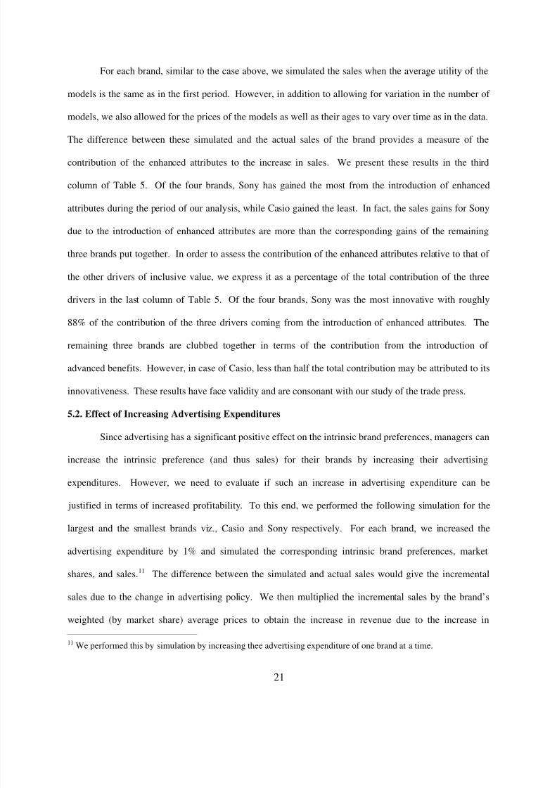
For each brand, similar to the case above, we simulated the sales when the average utility of the
models is the same as in the first period. However, in addition to allowing for variation in the number of
models, we also allowed for the prices of the models as well as their ages to vary over time as in the data.
The difference between these simulated and the actual sales of the brand provides a measure of the
contribution of the enhanced attributes to the increase in sales. We present these results in the third
column of Table 5. Of the four brands, Sony has gained the most from the introduction of enhanced
attributes during the period of our analysis, while Casio gained the least. In fact, the sales gains for Sony
due to the introduction of enhanced attributes are more than the corresponding gains of the remaining
three brands put together. In order to assess the contribution of the enhanced attributes relative to that of
the other drivers of inclusive value, we express it as a percentage of the total contribution of the three
drivers in the last column of Table 5. Of the four brands, Sony was the most innovative with roughly
88% of the contribution of the three drivers coming from the introduction of enhanced attributes. The
remaining three brands are clubbed together in terms of the contribution from the introduction of
advanced benefits. However, in case of Casio, less than half the total contribution may be attributed to its
innovativeness. These results have face validity and are consonant with our study of the trade press.
5.2. Effect of Increasing Advertising Expenditures
Since advertising has a significant positive effect on the intrinsic brand preferences, managers can
increase the intrinsic preference (and thus sales) for their brands by increasing their advertising
expenditures. However, we need to evaluate if such an increase in advertising expenditure can be
justified in terms of increased profitability. To this end, we performed the following simulation for the
largest and the smallest brands viz., Casio and Sony respectively. For each brand, we increased the
advertising expenditure by 1% and simulated the corresponding intrinsic brand preferences, market
shares, and sales.11 The difference between the simulated and actual sales would give the incremental
sales due to the change in advertising policy. We then multiplied the incremental sales by the brand’s
weighted (by market share) average prices to obtain the increase in revenue due to the increase in
11 We performed this by simulation by increasing thee advertising expenditure of one brand at a time.

8/7/2019 Digicam Paper Final
http://slidepdf.com/reader/full/digicam-paper-final 24/38
22
advertising. We present a summary of the cumulative increase in advertising, and the resulting
cumulative increases in unit sales and revenue over the period of the data in Table 6. These results reveal
that Sony gains more, both in terms of increase in unit sales as well as in terms of percentage change in
sales, from the increase in advertising expenditure compared to Casio. However, it should be noted that a
1% increase in the advertising expenditure in case of Sony is about 13 times that of a corresponding
increase in case of Casio. In all cases, the increase in revenue that would accrue from the increased
advertising expenditure exceeds the extra expense. While this may look attractive, we should note that
only a fraction of the increased revenue would translate into extra profit for the firm. Assuming a 10%
profit margin, we computed the increase in profits due to the change in advertising policy.12 Under this
assumption, the increase in advertising is still profitable for both Casio and Sony. Further analysis
revealed that while Casio could have recovered the total extra advertising expense within the first two
months of the data, Sony would have done so in eight months. Overall, our analysis implies that it would
be worthwhile for Casio and Sony to increase their advertising expenditures. Especially, the small
advertising budget of Casio coupled with its declining sales and market share triggered by a decline in its
intrinsic brand preference, provide sufficient grounds for increasing its advertising outlay.
5.3. Effect of Exogenous Changes in Model Attributes
One of the characteristics of our model is that we can estimate the effect of modifying the level of
a product attribute on brand sales. Specifically, we take the perspective of a Casio manager. Faced with
declining sales, the manager needs to find ways of improving the brand’s performance. Our analysis
above revealed that the decline in Casio’s sales may be attributed to the decline in brand preferences.
Moreover, our results in the previous subsection reveal that Casio can increase its advertising expenditure
and still be profitable. An alternative way of improving the brand’s performance would be to introduce a
new model with modified attributes. Such a modification will have a positive effect on the inclusive
value of the brand and thus increase its attractiveness to consumers.
12 Bloomberg reports that the profit margin for digital cameras is around 10-15%. The profit margins will be aneven lower percentage of the retail prices to which we have access.
8/7/2019 Digicam Paper Final
http://slidepdf.com/reader/full/digicam-paper-final 25/38
23
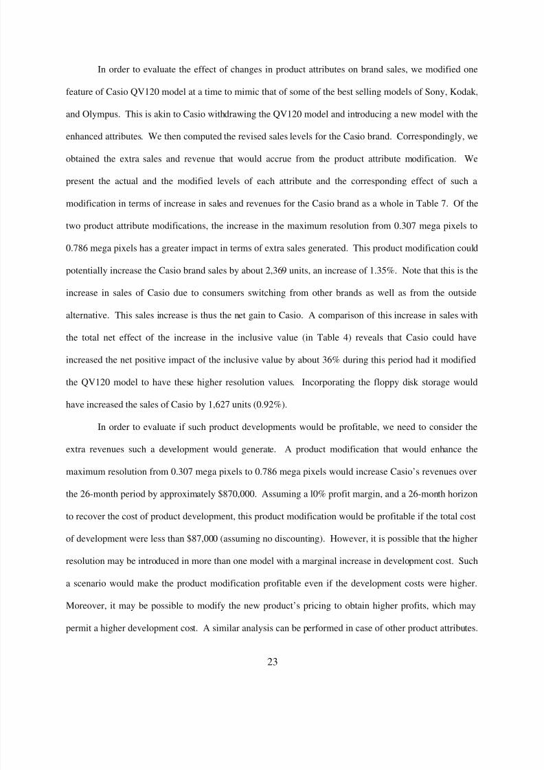
In order to evaluate the effect of changes in product attributes on brand sales, we modified one
feature of Casio QV120 model at a time to mimic that of some of the best selling models of Sony, Kodak,
and Olympus. This is akin to Casio withdrawing the QV120 model and introducing a new model with the
enhanced attributes. We then computed the revised sales levels for the Casio brand. Correspondingly, we
obtained the extra sales and revenue that would accrue from the product attribute modification. We
present the actual and the modified levels of each attribute and the corresponding effect of such a
modification in terms of increase in sales and revenues for the Casio brand as a whole in Table 7. Of the
two product attribute modifications, the increase in the maximum resolution from 0.307 mega pixels to
0.786 mega pixels has a greater impact in terms of extra sales generated. This product modification could
potentially increase the Casio brand sales by about 2,369 units, an increase of 1.35%. Note that this is the
increase in sales of Casio due to consumers switching from other brands as well as from the outside
alternative. This sales increase is thus the net gain to Casio. A comparison of this increase in sales with
the total net effect of the increase in the inclusive value (in Table 4) reveals that Casio could have
increased the net positive impact of the inclusive value by about 36% during this period had it modified
the QV120 model to have these higher resolution values. Incorporating the floppy disk storage would
have increased the sales of Casio by 1,627 units (0.92%).
In order to evaluate if such product developments would be profitable, we need to consider the
extra revenues such a development would generate. A product modification that would enhance the
maximum resolution from 0.307 mega pixels to 0.786 mega pixels would increase Casio’s revenues over
the 26-month period by approximately $870,000. Assuming a l0% profit margin, and a 26-month horizon
to recover the cost of product development, this product modification would be profitable if the total cost
of development were less than $87,000 (assuming no discounting). However, it is possible that the higher
resolution may be introduced in more than one model with a marginal increase in development cost. Such
a scenario would make the product modification profitable even if the development costs were higher.
Moreover, it may be possible to modify the new product’s pricing to obtain higher profits, which may
permit a higher development cost. A similar analysis can be performed in case of other product attributes.
8/7/2019 Digicam Paper Final
http://slidepdf.com/reader/full/digicam-paper-final 26/38
24
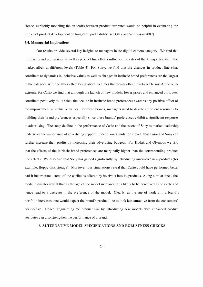
Hence, explicitly modeling the tradeoffs between product attributes would be helpful in evaluating the
impact of product development on long-term profitability (see Ofek and Srinivasan 2002).
5.4. Managerial Implications
Our results provide several key insights to managers in the digital camera category. We find that
intrinsic brand preferences as well as product line effects influence the sales of the 4 major brands in the
market albeit at different levels (Table 4). For Sony, we find that the changes in product line (that
contribute to dynamics in inclusive value) as well as changes in intrinsic brand preferences are the largest
in the category, with the latter effect being about six times the former effect in relative terms. At the other
extreme, for Casio we find that although the launch of new models, lower prices and enhanced attributes,
contribute positively to its sales, the decline in intrinsic brand preferences swamps any positive effect of
the improvement in inclusive values. For these brands, managers need to devote sufficient resources to
building their brand preferences especially since these brands’ preferences exhibit a significant response
to advertising. The steep decline in the performance of Casio and the ascent of Sony to market leadership
underscore the importance of advertising support. Indeed, our simulations reveal that Casio and Sony can
further increase their profits by increasing their advertising budgets. For Kodak and Olympus we find
that the effects of the intrinsic brand preferences are marginally higher than the corresponding product
line effects. We also find that Sony has gained significantly by introducing innovative new products (for
example, floppy disk storage). Moreover, our simulations reveal that Casio could have performed better
had it incorporated some of the attributes offered by its rivals into its products. Along similar lines, the
model estimates reveal that as the age of the model increases, it is likely to be perceived as obsolete and
hence lead to a decrease in the preference of the model. Clearly, as the age of models in a brand’s
portfolio increases, one would expect the brand’s product line to look less attractive from the consumers’
perspective. Hence, augmenting the product line by introducing new models with enhanced product
attributes can also strengthen the performance of a brand.
6. ALTERNATIVE MODEL SPECIFICATIONS AND ROBUSTNESS CHECKS
8/7/2019 Digicam Paper Final
http://slidepdf.com/reader/full/digicam-paper-final 27/38
25
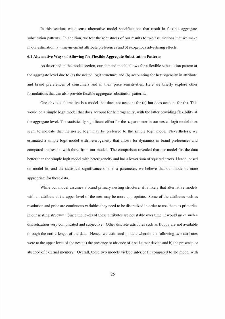
In this section, we discuss alternative model specifications that result in flexible aggregate
substitution patterns. In addition, we test the robustness of our results to two assumptions that we make
in our estimation: a) time-invariant attribute preferences and b) exogenous advertising effects.
6.1 Alternative Ways of Allowing for Flexible Aggregate Substitution Patterns
As described in the model section, our demand model allows for a flexible substitution pattern at
the aggregate level due to (a) the nested logit structure; and (b) accounting for heterogeneity in attribute
and brand preferences of consumers and in their price sensitivities. Here we briefly explore other
formulations that can also provide flexible aggregate substitution patterns.
One obvious alternative is a model that does not account for (a) but does account for (b). This
would be a simple logit model that does account for heterogeneity, with the latter providing flexibility at
the aggregate level. The statistically significant effect for the σ parameter in our nested logit model does
seem to indicate that the nested logit may be preferred to the simple logit model. Nevertheless, we
estimated a simple logit model with heterogeneity that allows for dynamics in brand preferences and
compared the results with those from our model. The comparison revealed that our model fits the data
better than the simple logit model with heterogeneity and has a lower sum of squared errors. Hence, based
on model fit, and the statistical significance of the σ parameter, we believe that our model is more
appropriate for these data.
While our model assumes a brand primary nesting structure, it is likely that alternative models
with an attribute at the upper level of the nest may be more appropriate. Some of the attributes such as
resolution and price are continuous variables they need to be discretized in order to use them as primaries
in our nesting structure. Since the levels of these attributes are not stable over time, it would make such a
discretization very complicated and subjective. Other discrete attributes such as floppy are not available
through the entire length of the data. Hence, we estimated models wherein the following two attributes
were at the upper level of the nest: a) the presence or absence of a self-timer device and b) the presence or
absence of external memory. Overall, these two models yielded inferior fit compared to the model with
8/7/2019 Digicam Paper Final
http://slidepdf.com/reader/full/digicam-paper-final 28/38
26
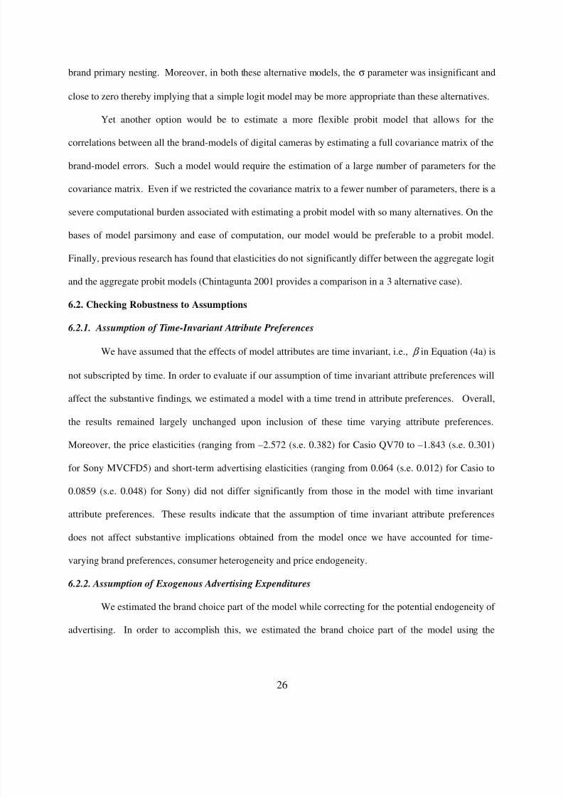
brand primary nesting. Moreover, in both these alternative models, the σ parameter was insignificant and
close to zero thereby implying that a simple logit model may be more appropriate than these alternatives.
Yet another option would be to estimate a more flexible probit model that allows for the
correlations between all the brand-models of digital cameras by estimating a full covariance matrix of the
brand-model errors. Such a model would require the estimation of a large number of parameters for the
covariance matrix. Even if we restricted the covariance matrix to a fewer number of parameters, there is a
severe computational burden associated with estimating a probit model with so many alternatives. On the
bases of model parsimony and ease of computation, our model would be preferable to a probit model.
Finally, previous research has found that elasticities do not significantly differ between the aggregate logit
and the aggregate probit models (Chintagunta 2001 provides a comparison in a 3 alternative case).
6.2. Checking Robustness to Assumptions
6.2.1. Assumption of Time-Invariant Attribute Preferences
We have assumed that the effects of model attributes are time invariant, i.e., β in Equation (4a) is
not subscripted by time. In order to evaluate if our assumption of time invariant attribute preferences will
affect the substantive findings, we estimated a model with a time trend in attribute preferences. Overall,
the results remained largely unchanged upon inclusion of these time varying attribute preferences.
Moreover, the price elasticities (ranging from –2.572 (s.e. 0.382) for Casio QV70 to –1.843 (s.e. 0.301)
for Sony MVCFD5) and short-term advertising elasticities (ranging from 0.064 (s.e. 0.012) for Casio to
0.0859 (s.e. 0.048) for Sony) did not differ significantly from those in the model with time invariant
attribute preferences. These results indicate that the assumption of time invariant attribute preferences
does not affect substantive implications obtained from the model once we have accounted for time-
varying brand preferences, consumer heterogeneity and price endogeneity.
6.2.2. Assumption of Exogenous Advertising Expenditures
We estimated the brand choice part of the model while correcting for the potential endogeneity of
advertising. In order to accomplish this, we estimated the brand choice part of the model using the
8/7/2019 Digicam Paper Final
http://slidepdf.com/reader/full/digicam-paper-final 29/38
27
control function approach (Petrin and Train 2004), which accounts for the endogeneity of the advertising
variable. Specifically, in a first stage, the endogenous variable (advertising) is regressed on its
instruments (in our case product attributes and their combinations). The residual from this regression is
then introduced as an additional regressor in the brand level model estimation. The results from this
analysis revealed that the estimates for the parameters at the brand level did not change significantly upon
accounting for the endogeneity of advertising. Moreover, the substantive results remained largely
unchanged. For example, after accounting for the potential endogeneity of advertising, the short-term
advertising elasticities for Casio, Olympus, and Sony were 0.0852 (s.e. 0.013), 0.0874 (s.e. 0.0232), and
0.1022 (s.e. 0.0471) respectively. These advertising elasticities are not significantly different from those
obtained under the assumption of exogenous advertising. Hence, we conclude that assuming the
advertising variable to be exogenous will not affect our main conclusions.
7. CONCLUSIONS
Our research addresses the following managerial questions: a) What are the relative importances
of intrinsic brand preferences, prices, product attributes, and number of models in driving the
performance of a brand? b) Does advertising play an important role in driving preferences? c) If so, would
it pay for brands to increase advertising spending? d) Under what circumstances would it be profitable for
brands to engage in product development efforts that would lead to an improvement in the attributes of
some of the existing models? Although set in the context of technology product markets, our model is
flexible enough to be used with data from consumer-packaged goods markets.
We find that intrinsic brand preferences have a much bigger effect on the performance of the
brand than the inclusive value which reflects model level prices, product attributes, and the length of the
brand’s product line. Further, we find that some brands can increase their advertising expenditures and
still increase their profitability. Casio, which has a relatively small advertising budget compared to the
other leading players in the market, could have done better by increasing its advertising investments.
Moreover, our analysis of the potential profit impact that would accrue from Casio improving some of its
8/7/2019 Digicam Paper Final
http://slidepdf.com/reader/full/digicam-paper-final 30/38
28
product attributes demonstrates the usefulness of our model in evaluating the feasibility and importance of
such developmental efforts.
Our approach is subject to several caveats and limitations addressing which may open up avenues
for future research. Although we account for the effects of model obsolescence as the age of the model
increases, our framework does not account for the dynamics in the consumer valuation of individual
attributes in any general way. The varying number of models offered by a brand in different time periods
complicates such an analysis. Although our framework can accommodate entry and exit of models, it
cannot easily be adapted to situations where brands enter or exit the market. Adding flexibility to our
model along these lines may be worthwhile. Additionally, while we model the effects of advertising on
the intrinsic brand preferences, data limitations do not permit the decomposition of the role that
advertising plays in informing consumers about new models from that of persuading consumers to buy
the existing product line. Such research objectives may be more easily pursued if one had access to
consumer level data rather than the aggregate data at our disposal. Besides, the introduction of models
with enhanced attributes may be accompanied by higher advertising expenditures. Correspondingly, we
may not have been able to accurately decompose the effects of the dynamics in brand preferences and the
changes in the brand’s product line. One can obtain a more accurate decomposition if advertising data at
the brand-model level were available. Moreover, our model assumes that the consumers notice all the
changes in the portfolio of models offered by a brand changes. However, due to limited cognitive
capacity, it is likely that the consumers only consider the models that are close to their needs and may
hence not be affected by the addition or withdrawal of other models. Moreover, it is likely that the
retailers do not carry all the models offered by the brand at all times. 13
We develop a demand model that captures the effects of changes in the portfolio of models
offered by a brand as well as the dynamics in its intrinsic preference on that brand’s performance and
assess its validity through an extensive simulation study. Our model parsimoniously incorporates the
information pertaining to all the models offered by a brand. Substantively, we provide insights into the
13 We thank an anonymous reviewer for pointing this out.
8/7/2019 Digicam Paper Final
http://slidepdf.com/reader/full/digicam-paper-final 31/38
29
relative importance of product line changes and dynamic brand preferences on the performance of a
brand. We also assess the returns on changes in advertising budgets as well as product development
efforts.
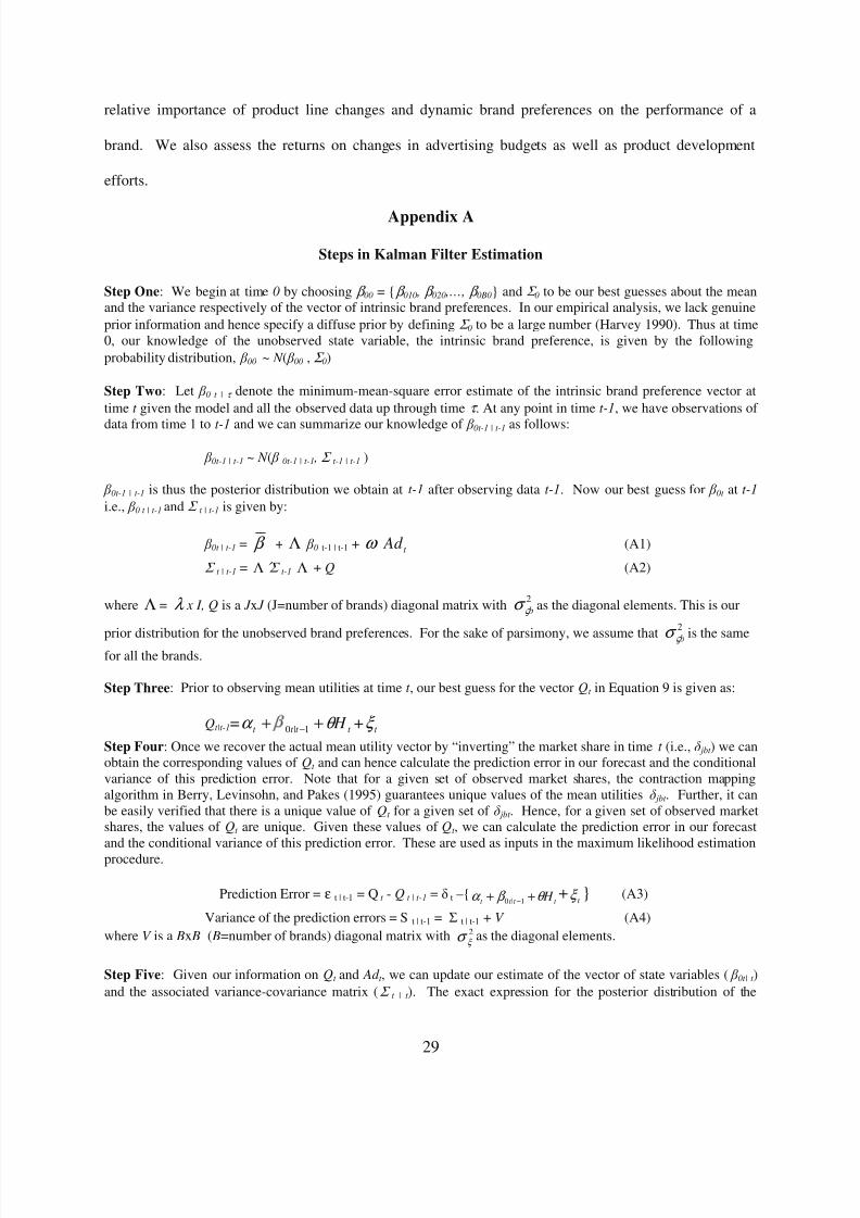
Appendix A
Steps in Kalman Filter Estimation
Step One: We begin at time 0 by choosing β 00 = { β 010 , β 020 ,…, β 0B0} and Σ 0 to be our best guesses about the meanand the variance respectively of the vector of intrinsic brand preferences. In our empirical analysis, we lack genuine
prior information and hence specify a diffuse prior by defining Σ 0 to be a large number (Harvey 1990). Thus at time0, our knowledge of the unobserved state variable, the intrinsic brand preference, is given by the following
probability distribution, 00 ~ N ( 00 , Σ 0)
Step Two: Let 0 t | τ denote the minimum-mean-square error estimate of the intrinsic brand preference vector at
time t given the model and all the observed data up through time τ . At any point in time t-1, we have observations of
data from time 1 to t-1 and we can summarize our knowledge of 0t-1 | t-1 as follows:
0t-1 | t-1 ~ N ( 0t-1 | t-1 , Σ t-1 | t-1 )
0t-1 | t-1 is thus the posterior distribution we obtain at t-1 after observing data t-1. Now our best guess for 0t at t-1
i.e., 0 t | t-1 and Σ t | t-1 is given by:
0t | t-1 = β + Λ 0 t-1 | t-1 + ω t Ad (A1)
Σ t | t-1 = Λ ′Σ t-1 Λ + Q (A2)
where Λ= λ x I, Q is a J x J (J=number of brands) diagonal matrix with2bς σ as the diagonal elements. This is our
prior distribution for the unobserved brand preferences. For the sake of parsimony, we assume that
2
bς σ is the samefor all the brands.
Step Three: Prior to observing mean utilities at time t , our best guess for the vector Qt in Equation 9 is given as:
Qt|t-1= t t t t H θ α ++−1|0 + t ξ
Step Four: Once we recover the actual mean utility vector by “inverting” the market share in time t (i.e., jbt ) we canobtain the corresponding values of Qt and can hence calculate the prediction error in our forecast and the conditionalvariance of this prediction error. Note that for a given set of observed market shares, the contraction mappingalgorithm in Berry, Levinsohn, and Pakes (1995) guarantees unique values of the mean utilities jbt . Further, it canbe easily verified that there is a unique value of Qt for a given set of jbt . Hence, for a given set of observed marketshares, the values of Qt are unique. Given these values of Qt , we can calculate the prediction error in our forecastand the conditional variance of this prediction error. These are used as inputs in the maximum likelihood estimation
procedure.
Prediction Error = ε t | t-1 = Q t - Q t | t-1 = t –{t t t t H θ β α ++ −1|0+
t ξ } (A3)
Variance of the prediction errors = S t | t-1 = Σ t | t-1 + V (A4)
where V is a Bx B ( B=number of brands) diagonal matrix with 2
ξ σ as the diagonal elements.
Step Five: Given our information on Qt and Ad t , we can update our estimate of the vector of state variables ( 0t| t )
and the associated variance-covariance matrix (Σ t | t ). The exact expression for the posterior distribution of the
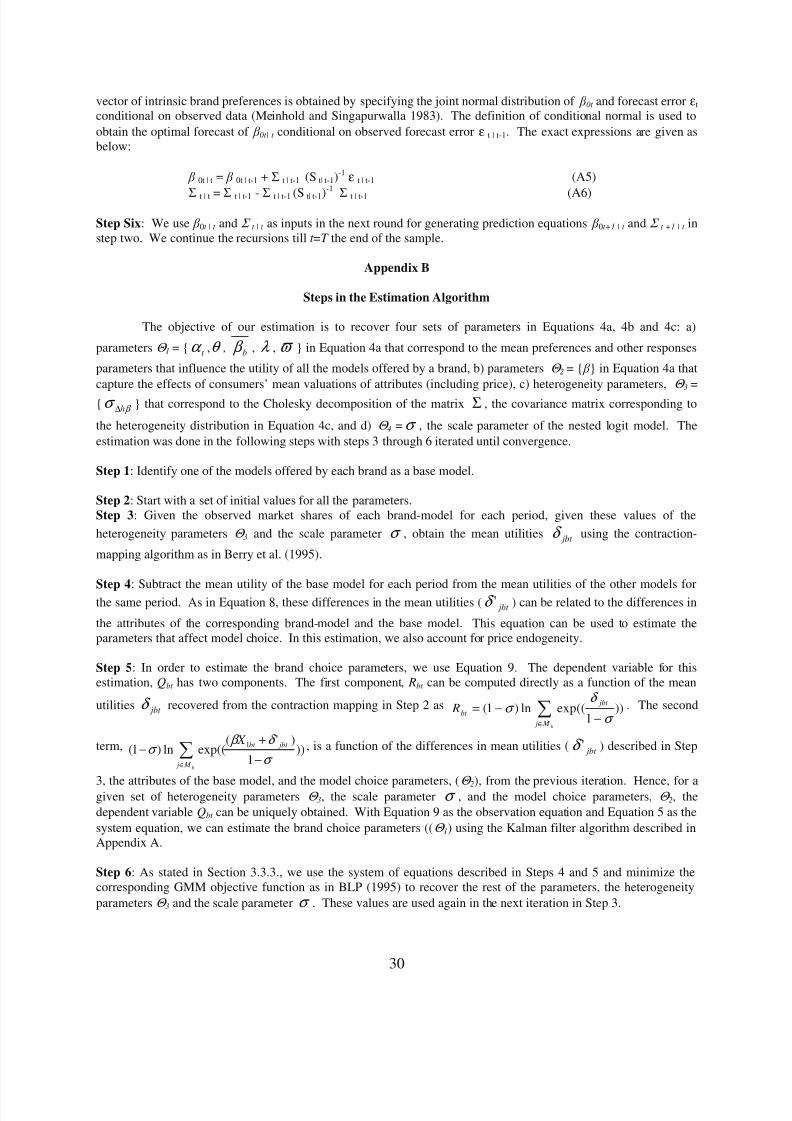
8/7/2019 Digicam Paper Final
http://slidepdf.com/reader/full/digicam-paper-final 32/38
30
vector of intrinsic brand preferences is obtained by specifying the joint normal distribution of 0t and forecast error εt conditional on observed data (Meinhold and Singapurwalla 1983). The definition of conditional normal is used to
obtain the optimal forecast of 0t| t conditional on observed forecast error ε t | t-1. The exact expressions are given asbelow:
0t | t = 0t | t-1 + Σ t | t-1 (S t| t-1)-1ε t | t-1 (A5)
Σ t | t = Σ t | t-1 - Σ t | t-1 (S t| t-1)-1
Σ t | t-1 (A6)
Step Six: We use 0t | t and Σ t | t as inputs in the next round for generating prediction equations 0t+1 | t and Σ t +1 | t instep two. We continue the recursions till t =T the end of the sample.
Appendix B
Steps in the Estimation Algorithm
The objective of our estimation is to recover four sets of parameters in Equations 4a, 4b and 4c: a)
parameters Θ 1 = { t α ,θ , b β , λ , ϖ } in Equation 4a that correspond to the mean preferences and other responses
parameters that influence the utility of all the models offered by a brand, b) parameters Θ 2 = { } in Equation 4a that
capture the effects of consumers’ mean valuations of attributes (including price), c) heterogeneity parameters, Θ 3 =
{ β σ h∆ } that correspond to the Cholesky decomposition of the matrix Σ , the covariance matrix corresponding to
the heterogeneity distribution in Equation 4c, and d) Θ 4 =σ , the scale parameter of the nested logit model. The
estimation was done in the following steps with steps 3 through 6 iterated until convergence.
Step 1: Identify one of the models offered by each brand as a base model.
Step 2: Start with a set of initial values for all the parameters.Step 3: Given the observed market shares of each brand-model for each period, given these values of the
heterogeneity parameters Θ 3 and the scale parameter σ , obtain the mean utilities jbt δ using the contraction-
mapping algorithm as in Berry et al. (1995).
Step 4: Subtract the mean utility of the base model for each period from the mean utilities of the other models forthe same period. As in Equation 8, these differences in the mean utilities ( jbt 'δ ) can be related to the differences in
the attributes of the corresponding brand-model and the base model. This equation can be used to estimate theparameters that affect model choice. In this estimation, we also account for price endogeneity.
Step 5: In order to estimate the brand choice parameters, we use Equation 9. The dependent variable for thisestimation, Qbt has two components. The first component, Rbt can be computed directly as a function of the mean
utilities jbt δ recovered from the contraction mapping in Step 2 as ∈ −
−=
b M j
jbt
bt R ))
1exp((ln)1(
σ
δ σ . The second
term, ∈
−
+−
b M j
jbt bt X ))
1
)'(exp((ln)1(
1
σ
δ β σ , is a function of the differences in mean utilities ( jbt 'δ ) described in Step
3, the attributes of the base model, and the model choice parameters, (Θ 2), from the previous iteration. Hence, for agiven set of heterogeneity parameters Θ 3, the scale parameter σ , and the model choice parameters, Θ 2, the
dependent variable Qbt can be uniquely obtained. With Equation 9 as the observation equation and Equation 5 as the
system equation, we can estimate the brand choice parameters ((Θ 1) using the Kalman filter algorithm described inAppendix A.
Step 6: As stated in Section 3.3.3., we use the system of equations described in Steps 4 and 5 and minimize thecorresponding GMM objective function as in BLP (1995) to recover the rest of the parameters, the heterogeneity
parameters Θ 3 and the scale parameter σ . These values are used again in the next iteration in Step 3.
8/7/2019 Digicam Paper Final
http://slidepdf.com/reader/full/digicam-paper-final 33/38
31
References
Akcura, Tolga M., Fusun Gonul, and Elina Petrova (2004), “Consumer Learning and Brand Valuation:
An Application on Over-the-Counter (OTC) Drugs,” Marketing Science, 23(4), 156-169.
Assmus, Gert, John Farley, and Donald Lehmann (1984), “How Advertising Affects Sales: A Meta-
Analysis of Econometric Results,” Journal of Marketing Research, 21(1), 65-74.
Bayus, Barry L., and William Putsis (1999), “Product Proliferation: An Empirical Analysis of
ProductLine Determinants and Market Outcomes,” Marketing Science, 18(2), 137-153.
Bell, David and Randolph Bucklin (1999), “The Role of Internal Reference Points in the Category
Purchase Decision,” Journal of Consumer Research, 26(3), 128-143.
Ben-Akiva, Moshe and Steven R. Lerman (1985), Discrete Choice Models: Theory and Application to
Travel Demand , The MIT Press, Cambridge, MA.
Berry, Steven T. (1994), "Estimating Discrete-Choice Models of Product Differentiation," Rand Journal
of Economics, 25, 242-262.
_____________, James Levinsohn, and Ariel Pakes (1995), "Automobile Prices in Market Equilibrium,"
Econometrica, 63(4), 841-890.
Chintagunta, Pradeep K. (2001), “Endogeneity and Heterogeneity in a Probit Demand Model: Estimating
Using Aggregate Data,” Marketing Science, 20(4), 442-456.
Draganska, Michaela and Dipak Jain (2005a), “Product-Line Length as a Competitive Tool,” Journal of
Economics and Management Strategy.
__________ and ___________ (2005b), “Consumer Preferences and Product-line Pricing Strategies: An
Empirical Analysis,” forthcoming in Marketing Science.
Fader, Peter S. and Bruce G. S. Hardie (1996), “Modeling Consumer Choice Among SKUs,” Journal of
Marketing Research, 33(4), 442-452.
Hamilton, James D. (1994), Time Series Analysis, Princeton University Press, Princeton, NJ.
Harvey, Andrew C. (1990), Forecasting, Structural Time Series Models and the Kalman Filter ,
Cambridge University Press.
Jedidi, Kamel, Carl F. Mela, and Sunil Gupta (1999). "Managing Advertising and Promotion for Long-
Run Profitability," Marketing Science, 18(1), 1-22.
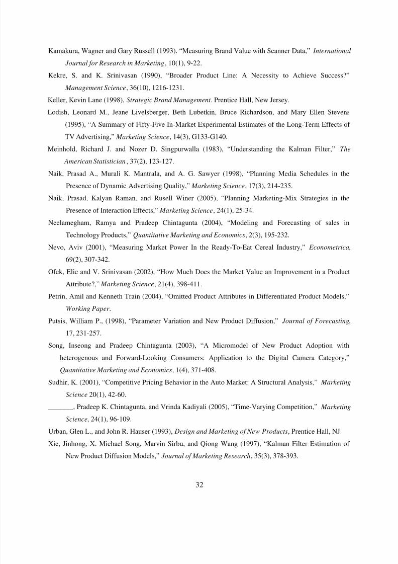
8/7/2019 Digicam Paper Final
http://slidepdf.com/reader/full/digicam-paper-final 34/38
32
Kamakura, Wagner and Gary Russell (1993). “Measuring Brand Value with Scanner Data,” International
Journal for Research in Marketing, 10(1), 9-22.
Kekre, S. and K. Srinivasan (1990), “Broader Product Line: A Necessity to Achieve Success?”
Management Science, 36(10), 1216-1231.
Keller, Kevin Lane (1998), Strategic Brand Management . Prentice Hall, New Jersey.
Lodish, Leonard M., Jeane Livelsberger, Beth Lubetkin, Bruce Richardson, and Mary Ellen Stevens
(1995), “A Summary of Fifty-Five In-Market Experimental Estimates of the Long-Term Effects of
TV Advertising,” Marketing Science, 14(3), G133-G140.
Meinhold, Richard J. and Nozer D. Singpurwalla (1983), “Understanding the Kalman Filter,” The
American Statistician , 37(2), 123-127.
Naik, Prasad A., Murali K. Mantrala, and A. G. Sawyer (1998), “Planning Media Schedules in the
Presence of Dynamic Advertising Quality,” Marketing Science, 17(3), 214-235.
Naik, Prasad, Kalyan Raman, and Rusell Winer (2005), “Planning Marketing-Mix Strategies in the
Presence of Interaction Effects,” Marketing Science, 24(1), 25-34.
Neelamegham, Ramya and Pradeep Chintagunta (2004), “Modeling and Forecasting of sales in
Technology Products,” Quantitative Marketing and Economics, 2(3), 195-232.
Nevo, Aviv (2001), “Measuring Market Power In the Ready-To-Eat Cereal Industry,” Econometrica,
69(2), 307-342.
Ofek, Elie and V. Srinivasan (2002), “How Much Does the Market Value an Improvement in a Product
Attribute?,” Marketing Science, 21(4), 398-411.
Petrin, Amil and Kenneth Train (2004), “Omitted Product Attributes in Differentiated Product Models,”
Working Paper .
Putsis, William P., (1998), “Parameter Variation and New Product Diffusion,” Journal of Forecasting,
17, 231-257.
Song, Inseong and Pradeep Chintagunta (2003), “A Micromodel of New Product Adoption with
heterogenous and Forward-Looking Consumers: Application to the Digital Camera Category,”
Quantitative Marketing and Economics, 1(4), 371-408.
Sudhir, K. (2001), “Competitive Pricing Behavior in the Auto Market: A Structural Analysis,” Marketing
Science 20(1), 42-60.
_______, Pradeep K. Chintagunta, and Vrinda Kadiyali (2005), “Time-Varying Competition,” Marketing
Science, 24(1), 96-109.
Urban, Glen L., and John R. Hauser (1993), Design and Marketing of New Products, Prentice Hall, NJ.
Xie, Jinhong, X. Michael Song, Marvin Sirbu, and Qiong Wang (1997), “Kalman Filter Estimation of
New Product Diffusion Models,” Journal of Marketing Research, 35(3), 378-393.
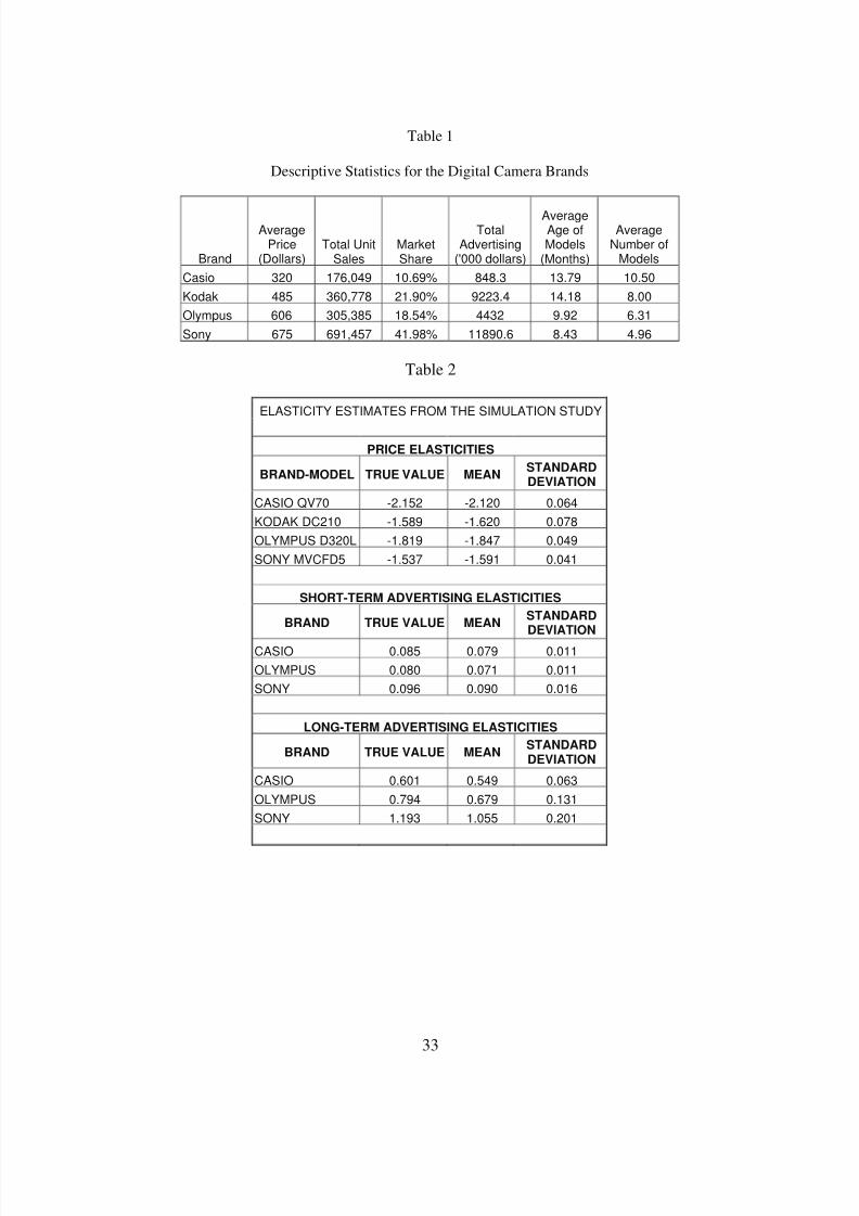
8/7/2019 Digicam Paper Final
http://slidepdf.com/reader/full/digicam-paper-final 35/38
33
Table 1
Descriptive Statistics for the Digital Camera Brands
Brand
AveragePrice
(Dollars)Total Unit
SalesMarketShare
TotalAdvertising
('000 dollars)
AverageAge ofModels
(Months)
AverageNumber of
Models
Casio 320 176,049 10.69% 848.3 13.79 10.50
Kodak 485 360,778 21.90% 9223.4 14.18 8.00
Olympus 606 305,385 18.54% 4432 9.92 6.31
Sony 675 691,457 41.98% 11890.6 8.43 4.96
Table 2
ELASTICITY ESTIMATES FROM THE SIMULATION STUDY
PRICE ELASTICITIES
BRAND-MODEL TRUE VALUE MEANSTANDARDDEVIATION
CASIO QV70 -2.152 -2.120 0.064
KODAK DC210 -1.589 -1.620 0.078
OLYMPUS D320L -1.819 -1.847 0.049
SONY MVCFD5 -1.537 -1.591 0.041
SHORT-TERM ADVERTISING ELASTICITIES
BRAND TRUE VALUE MEANSTANDARDDEVIATION
CASIO 0.085 0.079 0.011
OLYMPUS 0.080 0.071 0.011
SONY 0.096 0.090 0.016
LONG-TERM ADVERTISING ELASTICITIES
BRAND TRUE VALUE MEANSTANDARDDEVIATION
CASIO 0.601 0.549 0.063
OLYMPUS 0.794 0.679 0.131
SONY 1.193 1.055 0.201
8/7/2019 Digicam Paper Final
http://slidepdf.com/reader/full/digicam-paper-final 36/38
34
Table 3
Model Results
PARAMETER ESTIMATE SERR TVALUE
RESOLUTION 2.2582 0.489 4.6183
# OF IMAGES -0.4594 0.2982 -1.5406
FLOPPY 0.8312 0.3319 2.5041
EXTERNAL MEMORY -0.1541 0.1668 -0.9239
SELF TIMER 0.7867 0.1556 5.056
PRICE -2.1893 0.4308 -5.0822
AGE -2.2186 0.3201 -6.9305
MODEL CHOICECONDITIONAL ONBRAND CHOICE
AGE SQ 0.0137 0.084 0.1631
CARRYOVER 0.927 0.0692 13.3936
CONSTANT (CASIO) -0.4273 0.4918 -0.8688
CONSTANT (KODAK) -0.2457 0.4356 -0.564
CONSTANT (OLYMPUS) -0.3006 0.4367 -0.6884CONSTANT (SONY) -0.208 0.3934 -0.5287
ADVERTISING (CASIO) 1.1517 0.4998 2.3044
ADVERTISING (KODAK) 0.0007 0.0175 0.04
ADVERTISING (OLYMPUS) 0.1197 0.0705 1.6979
ADVERTISING (SONY) 0.2192 0.1194 1.8358
HOLIDAY 0.5386 0.1065 5.0588
BRAND CHOICE
SIGMA 0.9542 0.0247 38.6984
CASIO 0.0011 8.8212 0.0001
KODAK 0.0064 1.39772 0.00458
OLYMPUS 0.057 1.61982 0.03519
SONY 0.0337 2.59404 0.01299
RESOLUTION 0.4153 2.1948 0.1892
HETEROGENEITYPARAMETERS
PRICE 1.1029 0.4599 2.3979
Table 4
TOTAL EFFECT OF DYNAMICS ON UNIT SALES OF DIGITAL CAMERA BRANDS
NET EFFECT OF DYNAMICS ININCLUSIVE VALUE
NET EFFECT OF DYNAMICS INBRAND PREFERENCEBRAND
POSITIVE NEGATIVE POSITIVE NEGATIVE
CASIO 4,505 -398 1,590 -128,919
KODAK 9,973 -1,541 33,818 -8,418
OLYMPUS 14,421 -1,071 36,976 -12,788
SONY 60,182 -8 366,459 -780
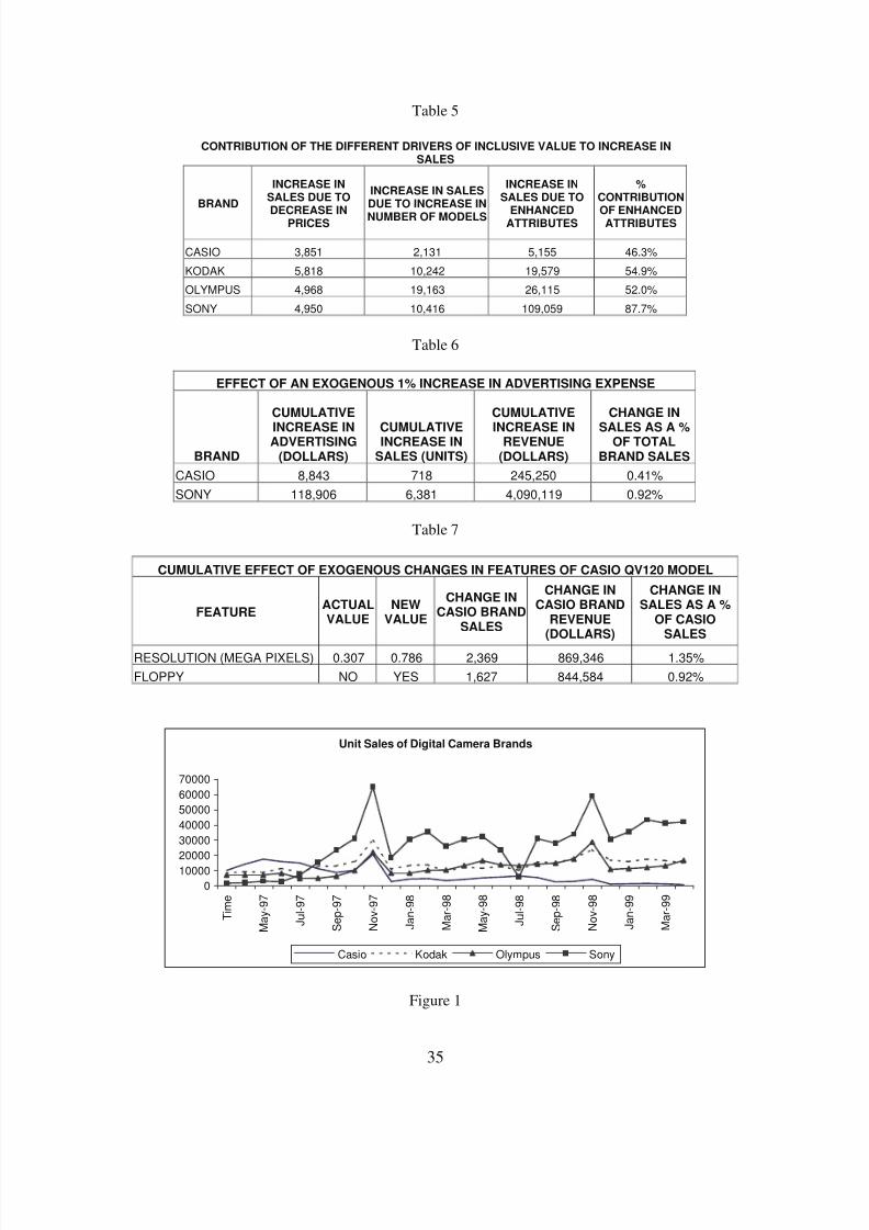
8/7/2019 Digicam Paper Final
http://slidepdf.com/reader/full/digicam-paper-final 37/38
35
Table 5
CONTRIBUTION OF THE DIFFERENT DRIVERS OF INCLUSIVE VALUE TO INCREASE INSALES
BRAND
INCREASE INSALES DUE TO
DECREASE INPRICES
INCREASE IN SALESDUE TO INCREASE IN
NUMBER OF MODELS
INCREASE INSALES DUE TO
ENHANCEDATTRIBUTES
%CONTRIBUTION
OF ENHANCEDATTRIBUTES
CASIO 3,851 2,131 5,155 46.3%
KODAK 5,818 10,242 19,579 54.9%
OLYMPUS 4,968 19,163 26,115 52.0%
SONY 4,950 10,416 109,059 87.7%
Table 6
EFFECT OF AN EXOGENOUS 1% INCREASE IN ADVERTISING EXPENSE
BRAND
CUMULATIVE
INCREASE INADVERTISING(DOLLARS)
CUMULATIVEINCREASE INSALES (UNITS)
CUMULATIVE
INCREASE INREVENUE(DOLLARS)
CHANGE IN
SALES AS A %OF TOTALBRAND SALES
CASIO 8,843 718 245,250 0.41%
SONY 118,906 6,381 4,090,119 0.92%
Table 7
CUMULATIVE EFFECT OF EXOGENOUS CHANGES IN FEATURES OF CASIO QV120 MODEL
FEATUREACTUALVALUE
NEWVALUE
CHANGE INCASIO BRAND
SALES
CHANGE INCASIO BRAND
REVENUE(DOLLARS)
CHANGE INSALES AS A %
OF CASIOSALES
RESOLUTION (MEGA PIXELS) 0.307 0.786 2,369 869,346 1.35%
FLOPPY NO YES 1,627 844,584 0.92%
Unit Sales of Digital Camera Brands
0
10000
20000
30000
40000
50000
60000
70000
T i m e
M a y - 9 7
J u l - 9 7
S e p - 9 7
N o v - 9 7
J a n - 9 8
M a r - 9 8
M a y - 9 8
J u l - 9 8
S e p - 9 8
N o v - 9 8
J a n - 9 9
M a r - 9 9
Casio Kodak Olympus Sony
Figure 1
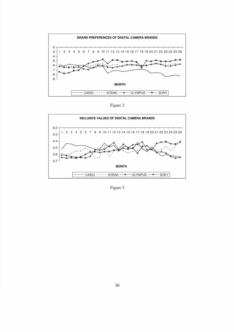
8/7/2019 Digicam Paper Final
http://slidepdf.com/reader/full/digicam-paper-final 38/38
BRAND PREFERENCES OF DIGITAL CAMERA BRANDS
-9
-8
-7
-6
-5
-4
-3
-2
1 2 3 4 5 6 7 8 9 10 11 12 13 14 15 16 17 18 19 20 21 22 23 24 25 26
MONTH
CASIO KODAK OLYMPUS SONY
Figure 2
INCLUSIVE VALUES OF DIGITAL CAMERA BRANDS
-0.7
-0.6
-0.5
-0.4
-0.3
-0.2
1 2 3 4 5 6 7 8 9 10 11 12 13 14 15 16 17 18 19 20 21 22 23 24 25 26
MONTH
CASIO KODAK OLYMPUS SONY
Figure 3
Related Documents