T.C. MARMARA UNIVERSITY FACULTY OF ENGINEERING METALLURGICAL AND MATERIALS ENGINEERING DEPARTMENT DIFFUSION PROPERTIES OF SELECTED MATERIALS Münevver BAYAZITLI (Metallurgical and Materials Engineering) SENIOR PROJECT ADVISOR Prof.Dr. Ersan KALAFATOĞLU İSTANBUL 2005

Welcome message from author
This document is posted to help you gain knowledge. Please leave a comment to let me know what you think about it! Share it to your friends and learn new things together.
Transcript

T.C. MARMARA UNIVERSITY
FACULTY OF ENGINEERING METALLURGICAL AND MATERIALS ENGINEERING
DEPARTMENT
DIFFUSION PROPERTIES OF SELECTED MATERIALS
Münevver BAYAZITLI
(Metallurgical and Materials Engineering)
SENIOR PROJECT
ADVISOR
Prof.Dr. Ersan KALAFATOĞLU
İSTANBUL 2005

2
TABLE OF CONTENTS
I. INTRODUCTION
II. BACKGROUND Diffusion Mechanisms
Steady-state Diffusion
Non-steady state Diffusion
Diffusion in gases
Diffusion in Liquids
Diffusion in solids
Diffusion Coefficient Measurements
III. PROCEDURE
IV. RESULTS
V. DISCUSSION OF RESULTS
VI. CONCLUSION
VII. REFERENCES

3
I.INTRODUCTION
The fragrance of flowers in a corner of a room drifts even to far distances.
When one droplet of ink is dripped into a cup of water, the ink soon spreads, even
without stirring, and quickly becomes invisible. These facts show that even if there is
no macroscopic flow in a gas or a liquid, molecular movement can take place, and
different entities can mix with each other.
It can be seen that examples of diffusion in everyday life are to much; the
diffusion of sugar in a cup of tea, the vaporization of water in a teakettle, cloud
formation, clothes drying, etc.
Engineers are concerned with diffusion when studying lots of subjects; such
as: gas absorption, seperation, crystallization and extraction, production and heat
treatment of metals, drying, cutting and welding metals, mass transfer in waste
treatment.
Many reactions and processes which are mentioned above, rely on the transfer
of mass either within a specific solid or from a liquid, a gas, or another solid phase.
This is accomplished by diffusion. The purpose of this project is to study the
properties of diffusion process, to observe the diffusion mechanisms and the diffusion
in gases, liquids and solids, to find the diffusion coefficient of selected materials by
doing experiments and using the formulas of diffusion.

4
II. BACKGROUND
DIFFUSION MECHANISMS
From an atomic perspective, diffusion is just the stepwise migration of atoms
from lattice site to lattice site. In fact, the atoms in solid materials are in constant
motion, rapidly changing positions. For an atom to make such a move, two
conditions must be met:
1. There must be an empty adjacent site.
2. The atom must have sufficient energy to break bonds with its neighbor
atoms and then cause some lattice distortion during the displacement (1).
This energy is vibrational in nature. At a specific temperature some small
fraction of the total number of atoms is capable of difusive motion, by virtue of the
magnitudes of their vibrational energies. This fraction increases with rising
temperature. Several different models for this atomic motion have been proposed; of
these posibilities, two dominates for metallic diffusion.
Vacancy Diffusion
One mechanism involves the interchange of an atom from a normal lattice
position to an adjacent vacant lattice site or vacancy, as represented in Figure 1. This
process necessitates the presence of vacancies, and the extent to which vacancy
diffusion can occur is a function of the number of these defects that are present;
significant concentrations of vacancies may exist in metals at elevated temperatures.
Since diffusing atoms and vacancies exchange positions, the diffusion of atoms in one
direction corresponds to the motion of vacancies in the opposite direction. Both self-
diffusion and interdiffusion occur by this mechanism.
Instertitial Diffusion
The second type of diffusion involves atoms that migrate from an instertitial
position to a neighboring one that is empty. This mechanism is found for
interdiffusion of impurities such as hydrogen, carbon, nitrogen, and oxygen, which
have atoms that are small enough to fit into the interstitial positions. Host or

5
substitutional impurity atoms rarely form instertitials and do not normally diffuse via
this mechanism. This phenomenon is appropriately termed instertitial diffusion,
shown in Figure 1.
Figure 1 schematic representation of vacancy and instertitial diffusion.
In most metal alloys, instertitial diffusion occurs much more rapidly than
diffusion by the vacancy mode, since the instertitial atoms are smaller, and thus more
mobile. Furthermore, there are emptier instertitial positions than vacancies; hence,
the probability of instertitial atomic movement is greater than for vacancy diffusion.
STEADY-STATE DIFFUSION
Diffusion is a time-dependent process that is, in macroscopic sense, the
quantity of an element that is transprted within another is a function of time. Often it
is necessary to know how fast diffusion occurs, or the rate of mass transfer. This rate
is frequently expresses as a diffusion flux (J), defined as the mass (or equivalently, the
number of atoms) M diffusing through and perpendicular to a unit cross-sectional area
of solid per unit time. In mathematical form, this may be represented as;
J = tA
M.
(Equation 1.a)
Where A denotes the area across which diffusion is occuring and t is elapsed diffusion
time. In differential form, this expression becomes;
J = dt
dMA1 (Equation 1.b)

6
The units for J are kilograms or atoms per meter squared per second (kg/m2-s or
atoms/m2-s).
If the diffusion flux does not change with time, a steady-state condition exists.
One common example of steady-state diffusion is the diffusion of atoms of a gas
through a plate of metal for which the concentrations (or pressures) of the diffusing
species on both surfaces of the plate are held constant. This is represented
schematically in Figure 2.a.
When concentration C is plotted versus position (or distance) within the solid
x, the resulting curve is termed the concentration profile; the slope at a particular
point on this curve is the concentration gradient:
Concentration gradient = dxdC (Equation 2.a)
Thin metal plane
PA>PB
and constant Gas at pressure PB
Gas at pressure PA Direction of diffusion of gaseous species Area, A Figure 2.a Steady-state difusion across a thin plane
Concentration of diffusing Species (C) CA CB Position (x) xA xB
Figure 2.b A linear concentration profile for the diffusion situation
7
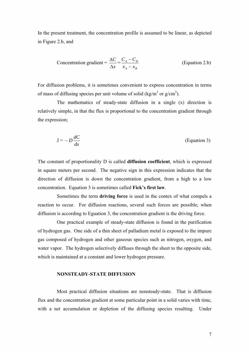
In the present treatment, the concentration profile is assumed to be linear, as depicted
in Figure 2.b, and
Concentration gradient = xC∆∆ =
BA
BA
xxCC
−−
(Equation 2.b)
For diffusion problems, it is sometimes convenient to express concentration in terms
of mass of diffusing species per unit volume of solid (kg/m3 or g/cm3).
The mathematics of steady-state diffusion in a single (x) direction is
relatively simple, in that the flux is proportional to the concentration gradient through
the expression;
J = dxdCD− (Equation 3)
The constant of proportionality D is called diffusion coefficient, which is expressed
in square meters per second. The negative sign in this expression indicates that the
direction of diffusion is down the concentration gradient, from a high to a low
concentration. Equation 3 is sometimes called Fick’s first law.
Sometimes the term driving force is used in the contex of what compels a
reaction to occur. For diffusion reactions, several such forces are possible; when
diffusion is according to Eguation 3, the concentration gradient is the driving force.
One practical example of steady-state diffusion is found in the purification
of hydrogen gas. One side of a thin sheet of palladium metal is exposed to the impure
gas composed of hydrogen and other gaseous species such as nitrogen, oxygen, and
water vapor. The hydrogen selectively diffuses through the sheet to the opposite side,
which is maintained at a constant and lower hydrogen pressure.
NONSTEADY-STATE DIFFUSION
Most practical diffusion situations are nonsteady-state. That is diffusion
flux and the concentration gradient at some particular point in a solid varies with time,
with a net accumulation or depletion of the diffusing species resulting. Under

8
conditions of nonsteady-state, use of Equation 3 is no longer convenient; instead, the
partial differential equation;
tC∂∂ = ⎟
⎠⎞
⎜⎝⎛
∂∂
∂∂
xCD
x. (Equation 4.1)
Known as Fick’s second law, is used. If the diffusion coefficient is independent of
composition, Equation 4.1 simplifies to;
tC∂∂ = 2
2
xCD
∂∂ (Equation 4.2)
Solutions to this expression are possible when physically meaningful boundary
conditions are specified. Comprehensive collections of these are given by Crank,
Carslaw and Jaeger.
One practically important solution is for a semi-infinite solid in which the
surface concentration is held constant. Frequently, the source of the diffusing species
is a gas phase, the partial pressure of which is maintained at a constant value.
Furthermore, the following assumptions are made (1):
1. Before diffusion, any of diffusing solute atoms in the solid are uniformly
distributed with concentration of C0.
2. The value of x at the surface is zero and increases with distance into the
solid.
3. The time is taken to be zero the instant before the diffusion process
begins.
DIFFUSION IN GASES
Diffusion through a Stagnant Gas Film
The Arnold diffusion cell of Figure 3, which is often used to measure mass
diffusivities experimentally, contains a pure liquid A which vaporizes and diffuses
into the stagnant column of gas B(3). Right at the liquid-gas interface the gas phase

9
concentration of A, expressed as mole fraction, is xA1. This is taken to be the gas
phase concentration of A corresponding to equilibrium with the liquid at the interface;
that is, xA1 is the vapor pressure of A divided by the total pressure, provided that A
and B from an ideal gas mixture. We further assume that the solubility of B in liquid
A is negligible (4).
At the top of the tube (z=z2) a stream of gas mixture A-B of concentration
xA2 flows past slowly; thereby the mole fraction of A at the top of the column is
maintained at xA2. The entire system is presumed to be held at constant temperature
and pressure. Gases A and B are assumed to be ideal.
Figure 3 Arnold diffusion cell
When the evaporating system attains a steady-state, there is a net motion of
A away from the evaporating surface and vapor B is stationary. Hence the expression
can be used for NAz:
AzN = dzdx
xcD A
A
AB
−−
1 (Equation 5.1)
A mass balance over an incremental column height ∆z states that at steady state;
0=− ∆+ zzAZzAz SNSN (Equation 5.2)
z = z1
z = z2
Liquid A
Gas stream of A and B
∆z

10
in which S is the cross sectional area of the column. Division by S∆z and taking the
limit as ∆z approaches zero gives;
0=−dz
dN Az (Equation 5.3)
Substitution of Eq.5.1 into Eq.5.3 gives;
01
=⎟⎟⎠
⎞⎜⎜⎝
⎛− dz
dxx
cDdzd A
A
AB (Equation 5.4)
For an ideal-gas mixture at constant temperature and pressure, c is constant,
and DAB is very nearly independent of concentration. Hence cDAB can be taken
outside the derivative to get;
01
1=⎟⎟
⎠
⎞⎜⎜⎝
⎛− dz
dxxdz
d A
A
(Equation 5.5)
This is a secon-order equation for the concentration profile expressed as mole fraction
of A. Integration with respect to z gives;
111 C
dzdx
xA
A
=−
(Equation 5.6)
A second integration then gives;
( ) 211ln CzCxA +=−− (Equation 5.7)
The two constants of integration may be determined by the use of the boundary
conditions;
B.C.1: at 1zz = , 1AA xx = (Equation 5.8)
B.C.2: at 2zz = , 2AA xx = (Equation 5.9)

11
When the constants so obtained are substituted into Eq.5.7, the following expressions
for the concentration profiles are obtained:
⎟⎟⎠
⎞⎜⎜⎝
⎛−−
111
A
A
xx =
12
1
1
2
11 zz
zz
A
A
xx −
−
⎟⎟⎠
⎞⎜⎜⎝
⎛−− (Equation 5.10)
Although the concentration prıofiles are helpful in picturing the diffusion
process, in engineering calculations it is usually the average concentration or the mass
flux at some surface that of interest(4).
The rate of mass transfer at the liquid-gas interface, which is the rate of
evaporation, is obtained by using Eq.5.1:
⎟⎟⎠
⎞⎜⎜⎝
⎛−
=+=−
−==1
2
1211
ln11
B
BABB
B
ABA
A
ABzzAz x
xzz
cDdz
dxx
cDdz
dxx
cDN (Equation 5.11)
DIFFUSION IN LIQUIDS
Mass diffusion in liquids is important to many industrial seperation
processes such as distillation and extraction. Often the largest resistance to overall
mass transfer is in the liquid phase. Diffusion coefficients in liquid systems are very
low when compared to gas systems. The low rates of diffusion in the liquid phase
make small effects, such as the volume change upon mixing, very important; the
precence of a concentratin gradient causes mass diffusion, but that rate may be
equally dependent upon other factors(2).
DIFFUSION IN SOLIDS
Diffusion coefficients in solids are much less than those in gases and range
from slightly less than those in liquids to very small. Diffusion in solids often occurs
in conjunction with adsorption and chemisorption phenomena. Metallurgists have
been interested in solid diffusion because of its importance in such problems as
degassing of metals and graphite, carburization, nitriding and phosphorizing of steel,

12
and desulfurization of steel. An example of diffusion coupled with adsorption is the
sulfur-iron system. It has been suggested that sulfur diffuses in iron by an alternate
dissociation and formation of sulfides, rather than by interpenetration or by place
change (2).
There have been many studies of the interdiffusion of metals. For instance,
it was known before 1900 that at 300 °C gold diffuses more rapidly through lead than
does sodium chloride through water at 18 °C. Radioactive tracers are convenient in
following interdiffusion in metals. Diffusion in polymers is another active research
area. The precence of vapors or gases sometimes alters the internal structure and
external dimensions of a polymer solid. Diffusion in polumers is of interest in the
drying dyeing of textiles, in the air or water permeability of paint films and packaging
materials, and the migration of plasticizers (2).
Diffusion in solid may be divided into two classes: structure-insensitive and
structure-sensitive diffusion. Structure-insensitive diffusion refers to the case in
which the solute is dissolved so as to form a homogeneous solution. An example is
the interdiffusion of metals, where the solute is part of the solid structure. The
copper-zinc system behaves in this manner, as does the lead-gold system. In contrast,
structure-sensitive diffusion occurs in the case of liquids and gases flowing through
the interstices and capillary passages in a solid; an example is the diffusive flow of
fluids through the sintered metal, such as that used in catalysts(2).
The Kirkendall Effect
An experiment which shows that, in a binary solid solution, each of the two
atomic forms can move with a different velocity. In the original experiment, as
performed by Smigalskas and Kirkendall, the diffusion of copper and zinc atoms was
studied in the composition range where zinc dissolves in copper and the alloy still
retains the face-centered cubic crystal structure characteristics of copper. Since their
original work, many other investigators have found similar results using a large
number of different binary alloys.

13
Figure 4 Kirkendall diffusion couple
Figure 4 is a schematic representation of a Kirkendall diffusion couple: a
three dimesional view of a block of metal formed by welding together two metals of
different compositions. In the plane of the weld, shown in the center of Figure 4, a
number of fine wires (usually of some refractory metal that will not dissolve in the
alloy system to be studied) are incorporated in the diffusion couple. These wires
serve as markers with which to study the diffusion process. For the sake of the
argument, assuming that the metals seperated by the plane of the weld are originally
pure metal A and pure metal B. In order to that a total amount of diffusion, which is
large enough to be experimentally measurable, can be obtained in a specimen of this
type, it is necessary that it be heated to temperature close to the melting point of the
metals comrising the bar, and maintained there for a relatively long time, usually of
the order of days, for diffusion in solids is much slower than in gases or liquids.
Upon cooling the specimen to room temperature, it is placed in a lathe and thin layers
parallel to the weld interface are removed from the bar. Each layer is then analyzed
chemically and the results plotted to give a curve showing the composition of the bar
as a function of distance along the bar (5).
DIFFUSION COEFFICIENT MEASUREMENTS
Marrero and Mason provide an excellent review of measurement techniques
for gas-phase diffusion coefficients. The Stefan method for the measurement of the
diffusion coefficient in gases uses the rate of evaporation of a liquid in a narrow tube.
The first component must be a liquid, while the second gas is passed across the top of
Metal A Metal B
Wire
Weld

14
the tube. The inside capillary diameter is known, and from the evaporation rate the
diffusion coefficient can be determined. Precision is poor at high or low vapor
pressures, and so the range of temperatures for a given system is restricted (2).
In the Loschmidt method, two gaseous components are olaced in a tube that
is divided into two sections by a removable partition. The partition is removed for a
time and the gases are allowed to diffuse under unsteady-state conditions. The
partition is reinserted and the contents of each chamber are analyzed. From this, the
diffusion coefficient can be calculated. The method often yields diffusion coefficients
that are in error because of convection currents. If the gases have different densities,
then there may be appreciable mass transfer by natural convection currents (2).
The point source method fo gases, developed by Walker and Westenberg,
has been used to measure diffusion coefficients at temperatures up to 1200 K with a
precision of about 1 percent. The point source method injects a trace sample of one
gas into the laminar flow of a second gas stream. In a flow system it is relatively easy
to control the temperature by adding a constant amount of heat to a constant flow of
gas. In the region of the injection probe, the total pressure may be asumed constant,
and the injected species diffuses along the direction of flow as well as in a radial
direction. The concentration of the injevted gas is measured by a special sampling
technique in which the gas ample is continually withdrawn and passed through a
thermal conductivity cell. The point source technique appears to be the most
satisfactory technique developed so far for measurements of diffusion coefficients
over wide ranges of temperature and pressure. The Stefan method was severely
limited by the requirement that one component be a liquid with vapor pressure neither
too high or too low, and the Loschmidt method, while capable of high temperature
measurements, is relatively imprecise even with the best available constant-
temperature equipment(2).
Diffusion coefficients in liquids are of interest not only to engineers
designing mass transfer equipment but also to physical chemists and others studying
the proporties of proteins and other high molacular weight polymer and colloid
solutions(2).

15
III. PROCEDURE
Experimental Plan for Gas Diffusion
Three laboratory solvents will be used in this experiment. These are water,
ethanol, methanol and isopropyl alcohol.
The solvents are put into the graduated cylinder which is on a proper mass
balance device. When the liquid is evaporating into the air, we can say the liquid
level at z=z1 as shown in Figure 5;
z = z2 2AA xx =
z = z1 1AA xx =
Liquid A Figure 5 Schematic illustration of the diffusion cell
The system is presumed to be held at constant temperature and pressure. With
time there is a net motion of liquid away from the surface and the weight and the
height of the liquid in the graduated cylinder decreases.
The mass change and the height of the liquid with increasing time will be
recorded. Temperature and pressure will be measured.
Vapor pressure of the liquid A is a function of temperature and will be found.
The mass diffusivity (cm2sec-1) of the selected solvent will be obtained by
using some formulas which are shown in the calculation part.

16
IV. RESULTS Measured values which are obtained from the experiment with water, ethanol,
isopropyl alcohol and methanol; are shown in the Table 1, Table 2, Table 3, and Table
4, respectively.
Decrease in the mass of substance with time and the increase in the height of
the graduated cylinder from the top to the level of liquid, with time are shown in the
graphs below (Figures 6, 7, 8, 9, 10, 11, 12, 13)

17
Result of experiment with pure water: Table 1 Results of pure water
t (min) Mass (g) H (mm) Temperature (°C) Humidity (%) 0 108.5235 142.5 22 49
60 108.5146 143 20 49 120 108.5099 143.5 20 49 180 108.5035 144 20 49 240 108.5005 144.1 20 49 300 108.4977 144.2 20 49
pure water
108,5235
108,5146108,5099
108,5035108,5005
108,4977y = -0,00008462x + 108,52097619
108,4900
108,4950
108,5000
108,5050
108,5100
108,5150
108,5200
108,5250
108,5300
0 60 120 180 240 300
Time (min.)
Mas
s (g
ram
Figure 6 Measured mass-time graph of pure water
pure water
142,5
143
143,5
144 144,1 144,2y = 0,0059x + 142,67
142
142,5
143
143,5
144
144,5
145
0 60 120 180 240 300
Time (min.)
Hei
ght o
f the
cyc
linde
r(m
m)
Figure 7 Measure height-time graph for pure water
18
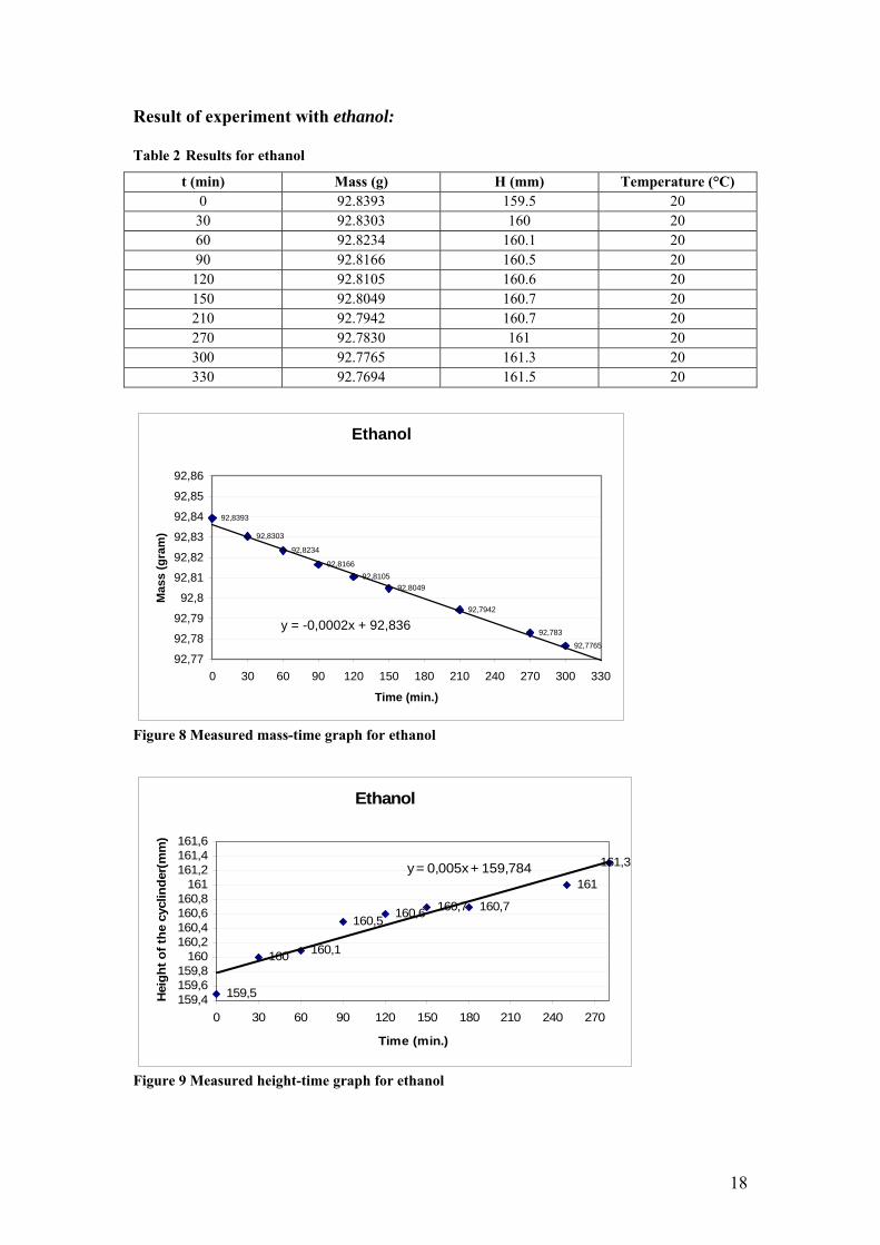
Result of experiment with ethanol: Table 2 Results for ethanol
t (min) Mass (g) H (mm) Temperature (°C) 0 92.8393 159.5 20
30 92.8303 160 20 60 92.8234 160.1 20 90 92.8166 160.5 20 120 92.8105 160.6 20 150 92.8049 160.7 20 210 92.7942 160.7 20 270 92.7830 161 20 300 92.7765 161.3 20 330 92.7694 161.5 20
Ethanol
92,8393
92,8303
92,8234
92,816692,8105
92,8049
92,7942
92,783
92,7765
y = -0,0002x + 92,836
92,77
92,78
92,79
92,8
92,81
92,82
92,83
92,84
92,85
92,86
0 30 60 90 120 150 180 210 240 270 300 330
Time (min.)
Mas
s (g
ram
)
Figure 8 Measured mass-time graph for ethanol
Ethanol
159,5
160 160,1
160,5 160,6 160,7 160,7
161
161,3y = 0,005x + 159,784
159,4159,6159,8
160160,2160,4160,6160,8
161161,2161,4161,6
0 30 60 90 120 150 180 210 240 270
Time (min.)
Hei
ght o
f the
cyc
linde
r(m
m)
Figure 9 Measured height-time graph for ethanol

19
Result of experiment with isopropyl alcohol:
Table 3 Results for isopropyl alcohol
t(min) Mass (g) H (mm) Temperature (°C) 0 87.5235 171 20
30 87.5078 171.2 20 60 87.5020 171.3 20 90 87.4974 171.4 20 120 87.4903 171.5 20 150 87.4848 171.6 20 180 87.4768 171.65 20 210 87.4715 171.7 20 240 87.4647 171.75 20 270 87.4623 171.8 20
Figure 10 Measured mass-time graph for isopropyl alcohol
Izopropyl Alcohol
171
171,2171,3
171,4171,5
171,6171,65
171,7171,75
171,8y = 0,0028x + 171,11
170,9171
171,1171,2171,3171,4171,5171,6171,7171,8171,9
172
0 30 60 90 120 150 180 210 240 270
Time (min.)
Hei
ght o
f the
cyl
inde
r(m
m)
Figure 11 Measured height-time graph for isopropyl alcohol
Izopropyl Alcohol
87,5235
87,507887,502
87,497487,4903
87,484887,4768
87,471587,464787,4623y = -0,0002x + 87,5174
87,44
87,46
87,48
87,5
87,52
87,54
0 30 60 90 120 150 180 210 240 270
Time (min.)
Mas
s (g
ram
)

20
Result of experiment with methanol: Table 4 Results for methanol
t (min) Mass (g) Height (mm) Temperature (°C) 0 94.8647 152.5 20 60 94.8160 153.5 20 90 94.7967 153.6 20 120 94.7768 153.7 20 150 94.7641 153.8 20 180 94.7380 154 20 240 94.6985 154.1 20 300 94.6613 154.2 20 360 94.6232 154.5 20
Methanol
94,8647
94,816
94,7768
94,738
94,6985
94,6613
94,6232y = -0,0007x + 94,85994,6
94,65
94,7
94,75
94,8
94,85
94,9
0 60 120 180 240 300 360 420
Time (min.)
Mas
s (g
ram
)
Figure 12 Measured mass-time graph for methanol
Methanol
152,5
153,5153,7
154 154,1 154,2
154,5y = 0,0046x + 152,95
152
152,5
153
153,5
154
154,5
155
0 60 120 180 240 300 360 420
Time (min.)
Hei
ght o
f the
cyc
linde
r(m
m)
Figure 13 Measured height-time graph for methanol

21
Calculations of Diffusion Coefficients:
Before calculation the diffusion coefficients of these solvents, some
calculations should be done. To calculate the diffusion flux, which is shown in the
Equation 6, the slope of the mass-time graph ( tM ∆∆ ) can be used. AM is the
molecular weight of the substances and A is the cross-sectional area of the graduated
cylinder which has a radius of 1 cm.
AtMMN A
.∆∆
= (Equation 6)
To obtain a diffusion coefficient, the equilibrium concentration (c) on the
liquid level should be known. It can be calculated by dividing the total atmospheric
pressure which is assumed as 1 atm, to the constant R ( KmolcmatmR ..06.82 3= )
times temperature (K).
At the top of the graduated cylinder, the concentration ( 2Ax ) of the ethanol,
isopropyl alcohol and methanol is zero. The concentration of pure water at the top, is
not zero. To calculate the concentration, the humidity should be known. As it can be
seen from Table1, humidity is %49 and this value can be used when calculating the
concentration at the top.
z∆ can be found from the difference between 2z and 1z level of the tube.
Finally, the diffusion coefficient of the laboratory solvents at 20°C can be
calculated from the equation below;
( )12ln..
BBAB xxc
zND ∆= (Equation 7)
All calculations and the results are shown in Table 5.

22
Table 5 Results of the experiment
Calculated Values
Pure Water
Ethanol
Isopropyl
Alcohol
Methanol
tM ∆∆ 0.0000846 0.0002 0.0002 0.0007
3cmgM A = 18 46 60 32
A ( 2cm ) 7.065 7.065 7.065 7.065
N (flux)
91008.11 −× 91025.10 −× 91086.7 −× 9106.51 −×
c (equilibrium concentration)
510159.4 −× 510159.4 −× 510159.4 −× 510159.4 −×
Vapor Pressure at 20°C 0.023079atm 0.05824atm 0.04367atm 0.12722atm
PPx AA =1 0.023079 0.05824 0.04367 0.12722
2Ax 0.00113087 0 0 0
11 1 AB xx −= 0.97692 0.94176 0.956 0.8727
22 1 AB xx −= 0.98869 1 1 1
( )12ln BB xx 0.0119 0.060 0.0449 0.136
z∆ (cm) 14.4 16.15 17.19 15.45
( )12ln..
BBAB xxc
zND ∆=
sec2cm
0.322 0.0663 0.0724 0.140

23
V. DISCUSSION OF RESULTS
Measurements and the diffusion coefficient values from the literature are
shown in the Table 6. Results of the experiment show that the measurements for pure
water and methanol can be possible at 20°C, but the measurements for ethanol and
isopropyl alcohol lower than the expected value. There can be lots of reasons for this
situation; temperature change in the atmosphere during the experiment, total
atmospheric pressure can be said.
Table 6 Diffusion Coefficients
Diffusion
Coefficient
Pure Water
Ethanol
Isopropyl Alcohol
Methanol
Experiment (at
20°C)
0.322 0.0663 0.0724 0.140
Literature(6) (at
0°C)
0.220 0.102 0.0808 0.132
VI. CONCLUSION
In conclusion, by studying with four laboratory solvents, the diffusion
properties of these substances were discussed. The basic diffusion mechanisms and
diffusion coefficient calculations were learned.

24
VII. REFERENCES
1. William D. CALLISTER; JR, Materials Science and Engineering an
Introduction, p.94, Fifth Edition, John Wiley Sons, Inc.
2. Robert S. BRODKEY, Harry C. HERSHEY; Transport Phenomena, A
Unified Approach; p.179, McGraw-Hill International Editions.
3. Leighton E. SISSOM, Donald R. PITTS; Elements of Transport
Phenomena; p.200, McGraw-Hill Book Company.
4. R. Byron BIRD, W.L. Stewart, and E.N. Lightfoot, Transport Phenomena,
p.525, John Wiley & Sons, Inc.
5. Physical Metallurgy Principles, p.386
6. John H. PERRY, Chemical Engineer’s Handbook, p.14-23, Fourth edition.
Related Documents