Diffusion Propagator Imaging: Using Laplace’s Equation and Multiple Shell Acquisitions to Reconstruct the Diffusion Propagator

Diffusion Propagator Imaging: Using Laplace’s

Equation and Multiple Shell Acquisitions toReconstruct the Diffusion Propagator

Maxime Descoteaux1, Rachid Deriche2, Denis Le Bihan1,Jean-Francois Mangin1, and Cyril Poupon1

1 NeuroSpin, IFR 49 CEA Saclay, France2 INRIA Sophia Antipolis - Mediterranee, France

Abstract. Many recent single-shell high angular resolution diffusionimaging reconstruction techniques have been introduced to reconstructorientation distribution functions (ODF) that only capture angular in-formation contained in the diffusion process of water molecules. By alsoconsidering the radial part of the diffusion signal, the reconstruction ofthe ensemble average diffusion propagator (EAP) of water molecules canprovide much richer information about complex tissue microstructurethan the ODF. In this paper, we present diffusion propagator imaging(DPI), a novel technique to reconstruct the EAP from multiple shell ac-quisitions. The DPI solution is analytical and linear because it is basedon a Laplace equation modeling of the diffusion signal. DPI is validatedwith ex vivo phantoms and also illustrated on an in vivo human braindataset. DPI is shown to reconstruct EAP from only two b-value shellsand approximately 100 diffusion measurements.

1 Introduction

One of the quest of diffusion-weighted (DW) imaging is the reconstruction ofthe full three-dimensional (3D) ensemble average propagator (EAP) describingthe diffusion process of water molecules in biological tissues. Many recent highangular resolution diffusion imaging (HARDI) techniques have been proposed torecover complex diffusion orientation distribution functions (ODF) of the whitematter geometry. However, these orientation functions derived from HARDI onlycapture the angular structure of the diffusion process on a single shell and aretherefore mostly useful for fiber tractography applications. The EAP can capturericher information by considering both radial and angular information part ofthe q-space diffusion signal. Thus, the EAP might provide means to infer axonaldiameter and also be sensitive to white matter anomalies [1].

In order to relate the observed diffusion signal to the underlying tissue mi-crostructure, we need to understand how the diffusion signal is influenced bythe tissue geometry and its properties. Under the narrow pulse assumption, therelationship between the diffusion signal, E(q), in q-space and the EAP, P (R),in real space, is given by an inverse Fourier transform (IFT) [3] as

J.L. Prince, D.L. Pham, and K.J. Myers (Eds.): IPMI 2009, LNCS 5636, pp. 1–13, 2009.c© Springer-Verlag Berlin Heidelberg 2009

2 M. Descoteaux et al.

P (R) =∫q∈�3

E(q)e−2πiq·Rdq, (1)

where E(q) = S(q)/S0 is the diffusion signal measured at position q in q-spaceand S0 is the baseline image acquired without any diffusion sensitization (q = 0).We denote q = |q| and q = qu, R = R0r, where u and r are 3D unit vectors, andq, R0 ∈ �. The wave vector q is q = γδG/2π, with γ the nuclear gyromagneticratio and G the applied diffusion gradient vector.

Various methods already exist to reconstruct the EAP [4,5,6,7,8,9,10,11,12].Among the most commonly used methods, diffusion tensor imaging (DTI) [4] islimited by the Gaussian assumption of the free diffusion model, which excludes ob-served in vivo phenomena such as restriction, heterogeneity, anomalous diffusion,and finite boundary permeability. Diffusion spectrum imaging (DSI) [5] can ac-count for DTI limitations. The technique has the advantage of beingmodel-free butrequires hundreds of DW measurements sampled on a dense Cartesian grid, whichrequires strong gradient fields, in order to evaluate the Fourier transform of Eq. 1.DSI was also shown to be possible on a non-Cartesian grid in [11] using less mea-surements on multiple spherical shells. More recently, inspired by computed to-mography, another technique was proposed to perform measurements along manyradial lines before computing 1D tomographic projections to reconstruct the 3DEAP [10]. This technique also requires hundreds of samples on a few radial lines ofq-space to recover the EAP. The results are promising but have not yet been ap-plied on an in vivo brain. Other techniques suggest using multiple spherical shellacquisitions in order to reconstruct the features of the EAP, such as generalizedhigh order tensors [6] based on cumulant expansions; or the composite and hin-dered restricted model of diffusion (CHARMED) [7]; or the diffusion kurtosis [8];or the diffusion orientation transform (DOT) [9]; or hybrid diffusion properties ofthe EAP [11]; or a fourth order Cartesian tensor representation of the probabilityprofile [12]. Unfortunately, for most of these methods, many DWmeasurements areneeded. Moreover, it remains unclear what is the right number of spherical shellsneeded and most of the results lack validation. Of all the mentioned techniques,DOT is in closer spirit to our approach and will be revisited later.

In this paper, we develop diffusion propagator imaging (DPI), a novel tech-nique for analytical EAP reconstruction from multiple shell acquisitions. Oursolution is simple, linear and compact. DPI is based on a 3D Laplace equationmodeling of the q-space diffusion signal, which greatly simplifies the solution toEq. 1 and allows one to obtain an analytical solution. An important part of thispaper is dedicated to validate DPI, both the signal fitting with Laplace equationand the EAP reconstruction, on real datasets from ex vivo phantoms [13]. Wealso illustrate DPI on a real in vivo human brain.

2 Diffusion Propagator Imaging (DPI)

q-Space Signal Approximation with Laplace’s Equation. Modeling the3D q-space diffusion signal to recover the EAP and capture complex fiber cross-ing configurations was proposed before in CHARMED [7] and DOT [9], where the

Diffusion Propagator Imaging: Using Laplace’s Equation 3

diffusion signal was modeled with multiple fiber compartments; in CHARMED,with a mixture of restricted and hindered compartements and in DOT, with amixture of exponential decay functions (mono-, bi or tri-exponential). In ourapproach, we do not want to assume any mixture models a priori. We seek asimpler representation of the diffusion signal that will naturally capture multipleshell measurements and allow for an analytical EAP solution.

Our main assumption is that the diffusion signal attenuation can be estimatedusing the 3D Laplace Equation. Under this assumption, we express the q-spacediffusion signal E(q) = S(q)/S0 in terms of any radius using the general or totalsolution of the Laplace equation in spherical coordinates, which gives

E(q) = E(qu) =∞∑

j=0

[cj

q�(j)+1+ djq

�(j)

]Yj(u) for q > 0, (2)

where �(j) is the order associated with element j of the spherical harmonic(SH) basis Yj , which is defined to be real and symmetric, and cj and dj are theunknown SH coefficients describing the signal. Also, for q = 0, E(q) = 1.

The Laplace equation requires boundary conditions. In our problem, we needat least two shell measurements and more diffusion measurements N than un-known coefficients to properly constrain Eq. 2. Intuitively, our Laplace equationmodeling can be seen as the heat equation between each given shell measure-ments, i.e. the solution is obtained when the heat does not change between thetemperature measurements given at each shell.

Analytical Diffusion Propagator Reconstruction. Under this Laplaceequation modeling assumption, we prove, in Appendix A, that the EAP canbe reconstructed as

P (R0r) = 2∞∑

j=0

(−1)�(j)/22π�(j)−1R�(j)−20

(2�(j) − 1)!!cjYj(r) for R0 > 0, (3)

where (n − 1)!! = (n − 1) · (n − 3) · . . . · 3 · 1. This expression is analytical andquite simple to compute. Note also that the EAP expression is linear and onlydepends on the cj coefficients, but the dj coefficients are nonetheless importantin the diffusion signal fitting/modeling procedure of Eq. 2. We finally note thatif R0 = 0, P (0) =

∫q∈�3 E(q)dq, the average diffusion signal in q-space.

3 Methods

As a starting point, we are given n HARDI shell datasets with the same numberof diffusion measurements N per shell. It is now standard in HARDI processingtechniques to use a modified real and symmetric SH basis of order � with elementsYj , where j := j(k, m) = (k2 + k + 2)/2 + m is defined from the order � andphase m standard SH Y m

� (see [14,15,16,17]).We can then generate the linear system associated with the Laplace equation

signal estimation given in Eq. 2. We let Sn be the N x 1 vector representing the

4 M. Descoteaux et al.

diffusion signal of shell number n at each of the N diffusion encoding gradientdirection. We also let C and D represent the R x 1 vectors of unknown SH coef-ficients, cj and dj in Eq. 2, where R = 1/2(�+1)(�+2). Next, we let B representthe N x R matrix constructed with the modified SH basis (as ine [14,15,16,17]).Finally, we define R�(q) = r� and I�(q) = r−�−1 to capture the regular andirregular radial part of the total Laplace equation. We can then construct thematrices of coefficients for each shell, Fn and Gn, as two R x R diagonal squarematrices with diagonal entries R�(j)(qn) and I�(j)(qn) respectively. As before, qn

is the q-value of shell n and �(j) is the order of the jth SH coefficient1.Lastly, for each of the n shell, we have the linear system Sn = BGnC+BFnD.

Combining all n systems, we obtain the general linear system representingEq. 2, S = AX. This system of over-determined equations is solved witha standard least-square solution yielding the vector X′ = [C′ D′]T, given byX′ = (ATA)−1ATS. Therefore, the estimated signal, S′, can be recovered sim-ply with AX′. We can then report the mean and standard deviation (std) ofthe Euclidean error |Sn − S′

n| percentage between the original and estimateddiffusion signal for each of the n shell and over all N diffusion measurements.

Finally, taking the first part of the estimated vector X′, we can extract the C′

coefficients needed to compute the EAP. The spherical function PR0 representingthe EAP for given R0, can be obtained with a simple matrix multiplication

PR0 = B

⎛⎝ . . .

2(−1)�(j)/22π�(j)−1R�(j)−20 /(2�(j) − 1)!!

. . .

⎞⎠C′, (4)

PR0 can then be visualized for different values of R0.

Data Acquisition. DPI was used to estimate the diffusion signal and theassociated EAP on ex vivo phantoms with fibers crossing at 90◦ and 45◦ designedin [13] with parameters: FOV=32cm, matrix 32x32, TH=14mm, TE=130ms,TR=4.5s,12.0s (45◦,90◦), BW=200KHz and b-values of 2000, 4000, 6000, 8000s/mm2 and 4000 uniformly distributed orientations. The number of directionswere also resampled to N = 15, 25 and 60 to test DPI under lower and morerealistic sampling schemes.

DPI was also applied on data acquired from a 3T Trio MR Siemens sys-tem, equipped with a whole body gradient (40 mT/m and 200 T/m/s) and an32 channel head coil. The acquisition parameters were TE/TR = 147ms/11.5s,BW=1680Hz/pixel, 96x96 matrix, isotropic 2mm resolution, and 60 axial slices.We acquired a b=0 diffusion image followed by four b-values acquisitions with64 uniform directions, at b = 1000, 2000, 4000 and 6000 s/mm2.

4 Results

Diffusion Propagator Imaging of the Ex Vivo Phantom. DPI is ap-plied on the 90 and 45 degree phantoms shown in Figure 1. We pick the center1 For j = {1, 2, 3, 4, 5, 6, 7, 8, ...}, �j = {0, 2, 2, 2, 2, 2, 4, 4, ...}.

Diffusion Propagator Imaging: Using Laplace’s Equation 5

(a) 902 (b) 452

Fig. 1. Physical phantoms designed in [13]. (a) 90◦ (photograph), and (b) 45◦ (fastspin-echo map and ROI)) phantoms. We also show the original diffusion signal equatorsperpendicular to the z (in blue, axial view) and x (in red, sagittal view) axes, fromb = 2000, 4000, 6000, and 8000 s/mm2, showing the diffusion signal decay.

Table 1. Mean and standard deviation of the percentage error in the multi-shell signalfit depending on the order � and number of measurements N used (sampling scheme)

(a) Estimation order �, multi-shell experiment with N = 4000shell 90◦ crossing 45◦ crossing

s/mm2 � = 2 � = 4 � = 16 � = 2 � = 6 � = 16

2000 9.4±2.5% 2.6±0.3% 2.5±0.3% 13±3.3% 2.0±0.2% 2.0±0.3%4000 16±3.9% 4.3±1.0% 4.3±1.1% 13±3.4% 3.9±0.7% 3.7±0.9%6000 18±4.4% 5.1±1.6% 4.5±1.1% 14±3.8% 5.2±1.2% 5.2±1.4%8000 20±6.5% 8.5±2.8% 8.5±3.0% 15±6.6% 8.5±2.7% 8.4±3.1%

(b) Sampling scheme N , multi-shell experimentshell 90◦ crossing, � = 4 45◦ crossing, � = 6

s/mm2 N = 4000 N = 60 N = 15 N = 4000 N = 60 N = 28

2000 2.6±0.3% 2.7±0.3% 2.8±0.4% 2.0±0.2% 2.1±0.2% 2.3±1.0%4000 4.3±1.0% 4.3±1.0% 5.1±1.4% 3.9±0.7% 4.0±0.8% 4.0±1.1%6000 5.1±1.6% 5.2±1.8% 6.2±2.6% 5.2±1.2% 5.3±1.3% 6.3±2.0%8000 8.5±2.8% 8.5±2.7% 8.6±3.2% 8.5±2.7% 8.5±2.5% 8.5±2.8%

voxel of the phantom, which contains approximately equal proportion of the twofiber branches of the crossing. The diffusion signal attenuation is also shown inFigure 1. In this visualization, red and blue lines illustrate equators of the orig-inal diffusion signal perpendicular to the x and z plan respectively, whereaslater, black lines illustrate the associated estimated signal in the signal fitexperiments.

Can Laplace’s Equation be used for diffusion signal estimation?Table 1 quantitatively shows that the diffusion signal can be modeled usingLaplace’s equation, on both ex vivo phantoms. This is qualitatively confirmed inFigure 2. From Table 1, we first see that estimation is accurate and that there isless than 10% mean signal fitting error with a small standard deviation at everyshell, for every estimation order � and every sampling scheme N . We also seethat the mean percentage error is increasing with increasing b-value. The mostsignificant error systematically occurs at shell b = 8000 s/mm2. This is due tothe intrinsic smoothness of the diffusion signal fit with Laplace’s equation. As

6 M. Descoteaux et al.

90◦ multi-shell, = 4 and N = 15 45◦ multi-shell, = 6 and N = 60

b = 2000 b = 4000 b = 6000 b = 8000 b = 2000 b = 4000 b = 6000 b = 8000

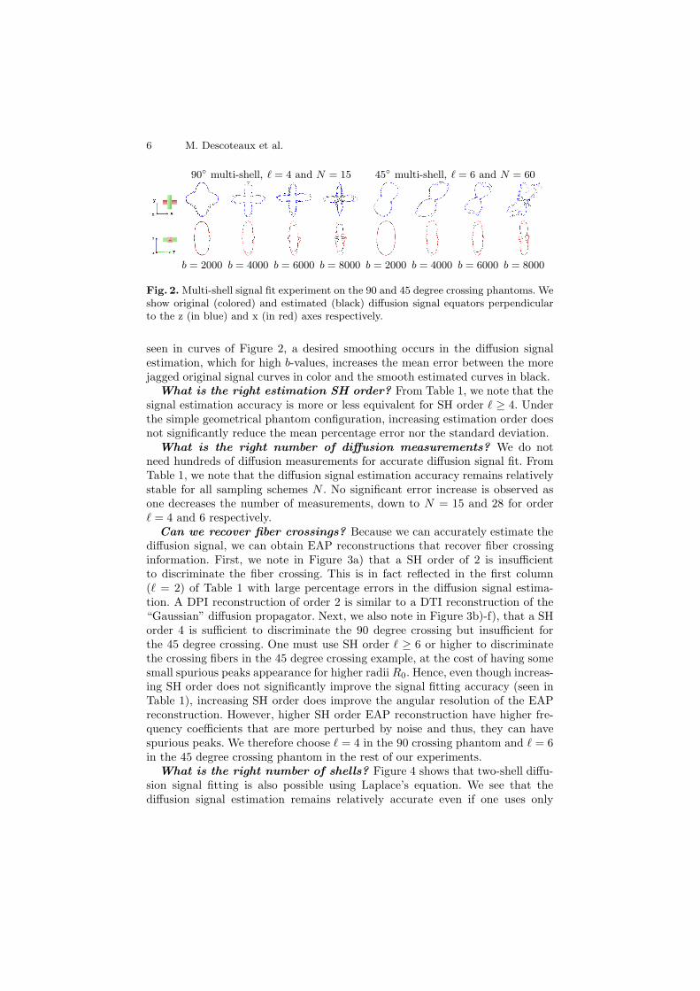
Fig. 2. Multi-shell signal fit experiment on the 90 and 45 degree crossing phantoms. Weshow original (colored) and estimated (black) diffusion signal equators perpendicularto the z (in blue) and x (in red) axes respectively.

seen in curves of Figure 2, a desired smoothing occurs in the diffusion signalestimation, which for high b-values, increases the mean error between the morejagged original signal curves in color and the smooth estimated curves in black.

What is the right estimation SH order? From Table 1, we note that thesignal estimation accuracy is more or less equivalent for SH order � ≥ 4. Underthe simple geometrical phantom configuration, increasing estimation order doesnot significantly reduce the mean percentage error nor the standard deviation.

What is the right number of diffusion measurements? We do notneed hundreds of diffusion measurements for accurate diffusion signal fit. FromTable 1, we note that the diffusion signal estimation accuracy remains relativelystable for all sampling schemes N . No significant error increase is observed asone decreases the number of measurements, down to N = 15 and 28 for order� = 4 and 6 respectively.

Can we recover fiber crossings? Because we can accurately estimate thediffusion signal, we can obtain EAP reconstructions that recover fiber crossinginformation. First, we note in Figure 3a) that a SH order of 2 is insufficientto discriminate the fiber crossing. This is in fact reflected in the first column(� = 2) of Table 1 with large percentage errors in the diffusion signal estima-tion. A DPI reconstruction of order 2 is similar to a DTI reconstruction of the“Gaussian” diffusion propagator. Next, we also note in Figure 3b)-f), that a SHorder 4 is sufficient to discriminate the 90 degree crossing but insufficient forthe 45 degree crossing. One must use SH order � ≥ 6 or higher to discriminatethe crossing fibers in the 45 degree crossing example, at the cost of having somesmall spurious peaks appearance for higher radii R0. Hence, even though increas-ing SH order does not significantly improve the signal fitting accuracy (seen inTable 1), increasing SH order does improve the angular resolution of the EAPreconstruction. However, higher SH order EAP reconstruction have higher fre-quency coefficients that are more perturbed by noise and thus, they can havespurious peaks. We therefore choose � = 4 in the 90 crossing phantom and � = 6in the 45 degree crossing phantom in the rest of our experiments.

What is the right number of shells? Figure 4 shows that two-shell diffu-sion signal fitting is also possible using Laplace’s equation. We see that thediffusion signal estimation remains relatively accurate even if one uses only

Diffusion Propagator Imaging: Using Laplace’s Equation 7

90◦, = 2, N = 4000, multiple shells (b = 2000, 4000, 6000, 8000 s/mm2)

a)

= 4, N = 4000, multiple shells (b = 2000, 4000, 6000, 8000 s/mm2)

b)

= 4, N = 15, two outermost shells (b = 2000, 8000 s/mm2)

c)

R0 = 0.1 μm 0.25 μm 0.5 μm 1 μm 2 μm 3 μm 5 μm 10 μm

45◦, = 4, N = 4000, multiple shells (b = 2000, 4000, 6000, 8000 s/mm2)

d)

= 8, N = 4000, multiple shells (b = 2000, 4000, 6000, 8000 s/mm2)

e)

= 6, N = 60, two outermost shells (b = 2000, 8000 s/mm2)

f)

R0 = 0.1 μm 0.25 μm 0.5 μm 1 μm 5 μm 10 μm 20 μm 50 μm

Fig. 3. EAP reconstruction on the 90◦ and 45◦ crossing phantom for different SH order�, sampling scheme N , number of shells, and radius R0

90◦ two-shell, � = 4 and N = 15 45◦ two-shell, � = 6 and N = 60

b = 2000 b = 4000 b = 6000 b = 8000 b = 2000 b = 4000 b = 6000 b = 8000

Fig. 4. Two-shell signal fit experiment on the 90◦ and 45◦ crossing phantoms usingshells b = 2000 and 8000 s/mm2

8 M. Descoteaux et al.

GFA map

RGB map from principal direction of the q-ball ODF

b = 1000 s/mm2 b = 2000 s/mm2 b = 4000 s/mm2 b = 6000 s/mm2

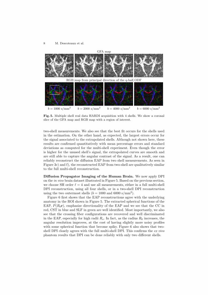
Fig. 5. Multiple shell real data HARDI acquisition with 4 shells. We show a coronalslice of the GFA map and RGB map with a region of interest.

two-shell measurements. We also see that the best fit occurs for the shells usedin the estimation. On the other hand, as expected, the largest errors occur forthe signal associated to the extrapolated shells. Although not shown here, theseresults are confirmed quantitatively with mean percentage errors and standarddeviations as computed for the multi-shell experiment. Even though the erroris higher for the unused shell’s signal, the extrapolated curves are smooth andare still able to capture the angular contrast of the signal. As a result, one canreliably reconstruct the diffusion EAP from two shell measurements. As seen inFigure 3c) and f), the reconstructed EAP from two-shell are qualitatively similarto the full multi-shell reconstruction.

Diffusion Propagator Imaging of the Human Brain. We now apply DPIon the in vivo brain dataset illustrated in Figure 5. Based on the previous section,we choose SH order � = 4 and use all measurements, either in a full multi-shellDPI reconstruction, using all four shells, or in a two-shell DPI reconstructionusing the two outermost shells (b = 1000 and 6000 s/mm2).

Figure 6 first shows that the EAP reconstructions agree with the underlyinganatomy in the ROI shown in Figure 5. The extracted spherical functions of theEAP, P (R0r), emphasize directionality of the EAP and we see that the CC inred, CST in blue and SLF in green are well identified. Most importantly, we alsosee that the crossing fiber configurations are recovered and well discriminatedin the EAP, especially for high radii Ro. In fact, as the radius R0 increases, theangular resolution improves, at the cost of having slightly more noisy profileswith some spherical function that become spiky. Figure 6 also shows that two-shell DPI closely agrees with the full multi-shell DPI. This confirms the ex vivophantom results that DPI can be done reliably with only two different shells.

Diffusion Propagator Imaging: Using Laplace’s Equation 9M

ulti-sh

ellD

PI

Tw

o-s

hel

lD

PI

EAP, R0 = 2μm EAP, R0 = 5μm

Fig. 6. DPI on the human brain dataset in the same crossing region as Figure 5. Inthe first row, a multi-shell DPI reconstruction and in the second row, a two-shell DPIwas done using the two outermost shells b = 1000 and 6000 s/mm2.

5 Discussion and Conclusions

The Laplace equation was successfully used to model the diffusion signal andreconstruct the EAP but a priori, there is no physical reason why this shouldbe. There might exist other possible model and family of functions to do so. Infact, [16] and [18] recently proposed new orthogonal bases to estimate the dif-fusion signal. In [16], the Spherical Polar Fourier (SFP) basis is used to extractfeatures of the EAP. The basis is composed of an angular part using sphericalharmonics and a radial part using an orthonormal radial basis function calledthe Gaussian-Laguerre polynomials. However, [16] do not have the full analyti-cal EAP reconstruction itself as we do. Only EAP features such as the ODF orother angular functions of the EAP can be computed. Separately, [18] proposed

10 M. Descoteaux et al.

to use Hermite polynomials to estimate the 1D q-space signal from spectroscopyimaging. While forming a complete orthogonal basis, the Hermite polynomialsalso have the important property that their Fourier transform can be expressedin terms of themselves. This property could potentially be very powerful to eval-uate Eq. 1. Although the Hermite polynomials were used for 1D q-space imaging,an extension to the 3D problem seems conceivable. One now has to think aboutthe best way to sample q-space (with Cartesian points, spherical shells, or ra-dial lines) in order to have sufficient measurements to robustly reconstruct theEAP and avoid the necessity for hundreds of measurements. Different samplingschemes might be better adapted depending on the chosen basis functions.

Our Laplace equation assumption also has several positive aspects that makeDPI an appealing technique. The advantages of DPI are threefold: i) The so-lution is analytical. ii) The signal modeling performs some level of smoothing.iii) The solution is linear and compact. First, having an analytical expressionfor the EAP allows one to estimate probability values outside the actual q-spacerange prescribed by the acquisition. In comparison, the DSI technique is limitedby the boundaries of q-space and thus, the reconstructed EAP is also bounded.Our approach is in closer spirit in with the DOT technique, where an expressionof P (R0r) is also obtained based on an exponential assumption of the signaldecay. A systematic comparison of DSI, DOT and DPI thus seems importantto highlight the limitations of the modeling and numerical versus analytical re-constructions. Next, as seen in the Result section, DPI performs some level ofsmoothing in the estimation. We believe this intrinsic smoothing of the Laplacemodeling is actually desired. Again, in comparison, DSI [5] uses a Hanning win-dow to smooth the signal before Fourier transform computation. No such low-pass filtering is needed for robust diffusion estimation and EAP reconstructionin DPI. Finally, the DPI solution is linear and quite compact, which makes theEAP reconstruction extremely fast; as fast as a simple least-square DTI or QBIreconstruction. DPI reconstruction runs in less than 2 minutes on a standardPC and its solution can be expressed in a small number of SH coefficients.

To conclude, we have introduced diffusion propagator imaging, a novel tech-nique for reconstructing the diffusion propagator from multiple shell acquisitions.We have shown that DPI can provide a new and efficient framework to studycharacteristics of the diffusion EAP, which opens interesting perspectives fortissue microstructure investigation. We now need to exploit DPI in clinical ac-quisitions and clinical settings. Future work will focus on new measures thatintegrate radial part of the diffusion signal, to lead to the development of newbiomarkers sensitive to white-matter anomalies, brain development and aging,and might also provide means to infer axonal diameter.

Acknowledgments. The authors are thankful to A. Ghosh and the diffusionMRI group of NeuroSpin for insightful discussion on the diffusion propagatorestimation. Moreover, thanks to K-H. Cho, Y-P. Chao and Pr. C-P. Lin for theirparticipation in he data acquisition. This work was supported by ProgrammeHubert Curien Orchid 2008 franco-taiwanais, l’Ecole des Neurosciences Paris-Ilede France (ENP), and l’Association France Parkinson for the NucleiPark project.

Diffusion Propagator Imaging: Using Laplace’s Equation 11

References

1. Cohen, Y., Assaf, Y.: High b-value q-space analyzed diffusion-weighted mrs andmri in neuronal tissues - a technical review. NMR Biomed. 15, 516–542 (2002)

2. Tuch, D.S.: Diffusion MRI of Complex Tissue Structure. PhD thesis, MassachusettsInstitute of Technology (2002)

3. Callaghan, P.T.: Principles of nuclear magnetic resonance microscopy. Oxford Uni-versity Press, Oxford (1991)

4. Basser, P., Mattiello, J., LeBihan, D.: Estimation of the effective self-diffusiontensor from the nmr spin echo. J. Magn. Reson. B 103(3), 247–254 (1994)

5. Wedeen, V.J., Hagmann, P., Tseng, W.Y.I., Reese, T.G., Weisskoff, R.M.: Mappingcomplex tissue architecture with diffusion spectrum magnetic resonance imaging.Magn. Reson. Med. 54(6), 1377–1386 (2005)

6. Liu, C., Bammer, R., Acar, B., Moseley, M.E.: Characterizing non-gaussian diffu-sion by using generalized diffusion tensors. Magn. Reson. Med. 51, 924–937 (2004)

7. Assaf, Y., Freidlin, R.Z., Rohde, G.K., Basser, P.J.: New modeling and experi-mental framework to characterize hindered and restrcited water diffusion in brainwhite matter. Magn. Reson. Med. 52, 965–978 (2004)

8. Jensen, J.H., Helpern, J.A., Ramani, A., Lu, H., Kaczynski, K.: Diffusional kurtosisimaging: The quantification of non- gaussian water diffusion by means of magneticresonance imaging. Magn. Reson. Med. 53, 1432–1440 (2005)

9. Ozarslan, E., Shepherd, T., Vemuri, B., Blackband, S., Mareci, T.: Resolution ofcomplex tissue microarchitecture using the diffusion orientation transform (dot).NeuroImage 31(3), 1086–1103 (2006)

10. Pickalov, V., Basser, P.: 3-D tomographic reconstruction of the average propagatorfrom MRI data. In: IEEE ISBI, pp. 710–713 (2006)

11. Wu, Y.C., Alexander, A.L.: Hybrid diffusion imaging. NeuroImage 36, 617–629(2007)

12. Barmpoutis, A., Vemuri, B.C., Forder, J.R.: Fast displacement probability profileapproximation from hardi using 4th-order tensors. In: IEEE ISBI, pp. 911–914(2008)

13. Poupon, C., Rieul, B., Kezele, I., Perrin, M., Poupon, F., cois Mangin, J.F.: Newdiffusion phantoms dedicated to the study and validation of hardi models. Magn.Reson. Med. 60, 1276–1283 (2008)

14. Hess, C., Mukherjee, P., Han, E., Xu, D., Vigneron, D.: Q-ball reconstruction ofmultimodal fiber orientations using the spherical harmonic basis. Magn. Reson.Med. 56, 104–117 (2006)

15. Tournier, J.D., Calamante, F., Connelly, A.: Robust determination of the fibreorientation distribution in diffusion mri: Non-negativity constrained super-resolvedspherical deconvolution. NeuroImage 35(4), 1459–1472 (2007)

16. Assemlal, H.E., Tschumperle, D., Brun, L.: Efficient computation of pdf-basedcharacteristics from diffusion mr signal. In: Metaxas, D., Axel, L., Fichtinger, G.,Szekely, G. (eds.) MICCAI 2008, Part II. LNCS, vol. 5242, pp. 70–78. Springer,Heidelberg (2008)

17. Descoteaux, M., Angelino, E., Fitzgibbons, S., Deriche, R.: Regularized, fast, androbust analytical q-ball imaging. Magn. Reson. Med. 58(3), 497–510 (2007)

18. Ozarslan, E., Koay, C.G., Basser, P.J.: Simple harmonic oscillator based estimationand reconstruction for one-dimensional q-space mr. In: ISMRM, p. 35 (2008)

12 M. Descoteaux et al.

A Proof of the Analytical Diffusion Propagator Solution

We want to prove that, under the Laplace equation assumption (Eq. 2), P (R0r)is given by Eq. 3. We need the following four identities: (1) The pointwise con-vergent expansion of the plane wave in spherical coordinates is given by

e±2πiq·R = 4π

∞∑j=0

(±i)�(j)j�(j)(2πqR0)Yj(u)Yj(r),

where jn is the spherical Bessel function (also used in the DOT derivation [9]).(2) We also need the following definite integral involving the Bessel function∫ ∞0

xmJn(x)dx = 2m(Γ (n/2 + m/2 + 1/2))/(Γ (n/2 − m/2 + 1/2)). Note how-ever that this integral blows up when the denominator is undefined, which occursin the specific case m = n + 1 because Γ (0) is undefined.(3) Hence, we need to solve property (2) in the special case that we have∫ ∞0 xnJn−1(x)dx. To do so, we need the following recurrence relation Jn−1(x) =

2n/xJn(x) − Jn+1(x). It is straightforward to show that the integral is zero.(4) Finally, Γ (n + 1/2) =

√π(2n − 1)!!/2n for n = 1, 2, 3, ..., where (2n − 1)!! =

1 · 3 · 5 · · · (2n − 1). For n = 0, Γ (1/2) =√

π.Now, we first write the 3D Fourier integral (Eq. 1) in spherical coordinates

P (R0r) =∫

E(q)e−2πiR0q·rdq =∫ ∞

q=0

∫|u|=1

q2E(qu)e−2πiR0qu·rdqdu. (5)

Using the pointwise convergent expansion of property (1) above, it implies that

P (R0r) = 4π

∞∑j=0

(−i)�(j)Yj(r)∫ ∞

q=0

∫|u|=1

q2E(qu)j�(j)(2πqR0)Yj(u)dqdu (6)

Next, we replace E(q) by the Laplacian equation given in Eq. 2 to obtain P (R0r)

4π

∞∑j=0

(−i)�(j)Yj(r)∫ ∫

q2∞∑

k=0

[ck

q�k+1+ dkq�k

]Yk(u)Yj(u)j�(j)(2πqR0)dqdu

Because the SH basis is orthonormal,∫

Yk(u)Yj(u)du = δkj . Also, since �(j) iseven in our basis, (−i)�(j) = (−1)�(j)/2. Finally, we use jn(x) =

√π/2xJn+1/2(x).

P (R0r) =2π√R0

∞∑j=0

(−1)�(j)2 Yj(r)

∫ ∞

0

(cj

q�(j)− 12

+ djq�(j)+ 3

2

)J�(j)+ 1

2(2πqR0)dq

︸ ︷︷ ︸I�(j)

(7)

I�(j) =∫ ∞

0

cjq1/2−�(j)J�(j)+1/2(2πqR0)dq

︸ ︷︷ ︸P1

+∫ ∞

0

djq�(j)+3/2J�(j)+1/2(2πqR0)dq

︸ ︷︷ ︸P2

Diffusion Propagator Imaging: Using Laplace’s Equation 13

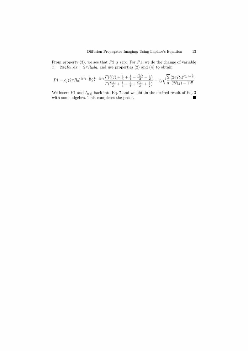
From property (3), we see that P2 is zero. For P1, we do the change of variablex = 2πqR0, dx = 2πR0dq, and use properties (2) and (4) to obtain

P1 = cj(2πR0)�(j)− 32 2

12−�(j) Γ (�(j) + 1

4 + 14 − �(j)

2 + 12 )

Γ ( �(j)2 + 1

4 − 14 + �(j)

2 + 12 )

= cj

√2π

(2πR0)�(j)− 32

(2�(j) − 1)!!

We insert P1 and I�(j) back into Eq. 7 and we obtain the desired result of Eq. 3with some algebra. This completes the proof. �